Abstract

Inference on overall ranking of a set of entities, such as chess players, subpopulations or hospitals, is an important problem. Estimation of ranks based on point estimates of means does not account for the uncertainty in those estimates. Treating estimated ranks without regard for uncertainty is problematic. We propose a Bayesian solution. It is competitive with recent frequentist methods, and more effective and informative, and is as easy to implement as it is to compute the posterior means and variances of the entity means. Using credible sets, we created novel credible distributions for the rank vector of the entities. We evaluate the Bayesian procedure in terms of accuracy and stability in two applications and a simulation study. Frequentist approaches cannot take account of covariates, but the Bayesian method handles them easily.

Keywords: Bayes; Credible sets; Fay-Herriot model; hierarchical Bayes; highest posterior density; small area estimation; unstructured Bayes.

1 Introduction

Reliable estimates of measures of important characteristics of agriculture, employment, health, education, for example, for various subpopulations are some of the important data produced by many national and international statistics offices around the world. For example, the United Nations Sustainable Development Goals, the US Small Area Income and Poverty Estimation (SAIPE) and many programs in European Union need accurate poverty data at disaggregated levels for making public policies and implementing welfare programs. Disaggregated levels may be defined by partitioning a particular population into several subpopulations. For example, subpopulations may refer to the states of a country (population). Effective implementations of many welfare programs and economic development policies critically need accurate point estimates of important characteristics at relevant subpopulation level. In this article we will also use “small areas” or “small domains” to refer to “subpopulations”. Definitely, the word “subpopulation” has a wider meaning. In a broader sense we use the word “entity” which may refer to a subpopulation or an individual. But in its place we will also use “small area” since our proposed solution to the problem of interest emerges from small area estimation methodology.

Productions of accurate estimates of the means for one or more characteristics for the subpopulations are usually the primary goals of many government agencies. However, inference on overall ranking of a set of entities, which may be individuals, small areas, hospitals, herds of animals, etc. is a problem of significant interest. Often it is crucially important to identify subpopulations with very low or high means of a characteristic. Effective implementation of welfare and well-being programs overseen by government or private organizations, identifying the better yielding crop varieties in agriculture research, or top-breeding sires in breeding research, etc. require reliable estimation of the rank vector. Due to limited resources government agencies may want to identify some of the most underprivileged or impoverished subpopulations to implement government programs to support those groups. Similarly, a business entity planning to open new locations would like to know the localities (or geographic regions) with the most demands for its products and services. In these cases, in addition to estimating the true subpopulation means, it is also important to accurately identify subpopulations that are either at the upper or at the lower end in terms of their means. This goal requires accurately estimating the ranks of several or all the subpopulations. According to Laird and Louis (1989), ranking can draw attention to unusually good or poor performance of some subpopulations. They noted that ranking of objects and entities arises in a wide variety of applications, and an appropriate solution provides an important tool to the investigators and policy makers setting priorities for the next stage of their investigations.

The importance of joint ranking of $m$ subpopulations with means $\theta_{1},\cdots,\theta_{m}$ of a common characteristic has been emphasized in a pioneering article by Klein et al. (2020) (we will subsequently also use the abbreviation KWW to refer to this paper or the method considered by these authors). Overall true ranks of the subpopulations are unknown as those are determined by the true unknown $\theta_{i}$’s. Klein et al. (2020) noted that ranking of populations, governmental units, teams, players, health service providers, etc. based on experimental, observational or “survey data are usually released without direct statistical statements of uncertainty on estimated overall rankings”. They emphasized that prior to their work national statistical agencies did not have any statistical methodology to account for uncertainty in their released estimates of overall rankings. They further cautioned that from published point estimates of the means with no explicit ranking, practitioners frequently use the point estimates to naively ascertain ranks of the subpopulations. Ranks determined this way, which are only point estimates, ignore any uncertainty in the estimates of the true means $\theta_{i}$’s as these estimates are invariably subject to error, sampling error is the most common. Different sets of estimates of $\theta_{i}$’s from different data sets will potentially lead to different sets of ranks of the subpopulations. Clearly, even the best possible estimators of small area means are subject to error due to the sampling variability of the estimators. It is thus both imperative and a sound policy to evaluate uncertainty associated with the reported ranks based on reasonable estimates of subpopulation means. Obviously, the accuracy of the estimated ranks can be appropriately studied through the joint distribution of the ranks, determined from the estimators of the means.

In an application to rank the fifty states of the U.S. and Washington, DC, using mean commuting times of workers sixteen or older and not working from home, Klein et al. (2020) used survey data collected from the American Community Survey (ACS). In their approach to the joint confidence set for the true rank vector, which they determine from an appropriate joint confidence set of the true means, the authors treated the unknown means as constants. They followed the classical approach to estimating the ranks where the true parameters $\theta_{i}$’s are considered to be fixed but unknown. Some of the early works on ranking and selection of population means are by Bechhofer (1954) and Gupta (1956) who adopted the frequentist approach (that is, the classical approach) to inference. While Klein et al. (2020) also used the frequentist approach for their application, they briefly mentioned in a remark that an analogous Bayesian version of their frequentist solution is possible. We have proposed here based on the Bayesian approach two novel and easily implementable solutions to this problem. Our proposed solutions enjoy better interpretation and based on some desirable measures (explained later) are at least as competitive as or better than the frequentist solution.

The Bayesian approach treats the unknown subpopulation means as random and assigns them a suitable joint distribution. Following the Bayesian approach to ranking of several binomial populations by Bland and Bratcher (1968), Govindarajulu and Harvey (1974) presented a unified Bayesian treatment of the ranking and selection problem. Goel and Rubin (1977) proposed a Bayesian approach on selecting a subset containing the best subpopulation. Laird and Louis (1989) used an empirical Bayes (EB) approach to the ranking problem to environmental monitoring of regions or health service providers suspected of elevated disease rates for residents or failure rates from services for patients, requiring attention to mitigate risks. Indeed Morris and Christiansen (1996) highlighted the utility of Bayesian approach to the ranking of hospitals. Unlike the frequentist approach, the EB and the Bayesian approaches facilitate hierarchical modeling of the random latent subpopulation means through regression on relevant available covariates. An early application of hierarchical modeling to ranking of subpopulations is due to Efron and Morris (1975). In their application to rank thirty-six cities of El Salvador based on prevalence of toxoplasmosis rates, they indicated the pitfall of ranking the cities using only observed estimates of the rates without paying attention to the variability of these estimates.

In the next section we provide a brief review of the relevant literature on ranking. We introduce two reasonable Bayesian models by specifying suitable joint prior distributions for the unknown subpopulation means. Corresponding to a prior distribution a Bayesian model is formed by augmenting the sampling distribution of the data, which is the cornerstone of the classical approach to a frequentist solution. In our Bayesian formulation, we consider two noninformative improper prior distributions. One prior distribution that provides no structure for the unknown $\theta_{i}$’s we consider it reasonable since joint credible sets for the $\theta_{i}$’s that are derived from the resulting posterior distribution exactly agree with the joint confidence sets of the $\theta_{i}$’s developed for the application by by Klein et al. (2020). The second prior distribution is based on a conjugate prior for the means leading to a widely used hierarchical model, introduced earlier by Fay and Herriot (1979), Berger (1985), Aitkin and Longford (1986), Berger and Deely (1988), Laird and Louis (1989) and Morris and Christiansen (1996). While most of these authors used an EB approach by estimating the parameters of the prior distribution in the hierarchical model, Berger and Deely (1988) and Morris and Christiansen (1996) used the hierarchical Bayes (HB) approach (or its approximation) by assigning reasonable noninformative improper priors to the model parameters. We follow these latter groups and will pursue a fully Bayesian (that is, HB) approach with similar improper priors on the model parameters. We add that whereas Berger and Deely (1988) and Morris and Christiansen (1996) used the HB approach for (point) estimation of individual ranks, we consider this approach for joint credible set of the overall mean vector by proposing a credible distribution through an innovative idea.

2 A selected review of the ranking literature and introduction of Bayesian models

Our motivation for this research has stemmed from a need to developing a Bayesian solution to the joint ranking problem proposed in a pioneering paper by Klein et al. (2020). A population may be partitioned into $m$ subpopulations. Suppose $\theta_{i}$ is the mean for certain characteristic of the $i$th subpopulation. In the application considered by Klein et al. (2020), they are interested in ranking 51 subpopulations, the fifty states of US and Washington, DC, based on $\theta_{i}$, the mean commuting times of the workers not working from home, $i=1,\cdots,m$. Similar to theirs, our goal is to make joint inference about the true ranks $\check{r}_{1},\cdots,\check{r}_{m}$, of the $m$ subpopulations based on estimators $Y_{1},\cdots,Y_{m}$ of $\theta_{1},\cdots,\theta_{m}$, and appropriate models. Alternatively, these $m$ subpopulations may refer to $m$ individuals. In ranking $\theta_{i}$’s we treat them continuous variables. We rank the $\theta_{i}$’s from the smallest to the largest, where the rank of $\theta_{i}$ is

$$\check{r}_{i}\equiv\check{r}_{i}(\theta)=\sum_{j=1}^{m}I(\theta_{j}\leq\theta_{i})=1+\sum_{j:j\neq i}I(\theta_{j}\leq\theta_{i}),~{}\mbox{for }i=1,\cdots,m.$$ (1)

The estimated overall ranking based on the estimators $Y_{1},\cdots,Y_{m}$ of $\theta_{1},\cdots,\theta_{m}$, is denoted by $R_{1},\cdots,R_{m}$, where

$$R_{i}=\sum_{j=1}^{m}I(Y_{j}\leq Y_{i})=1+\sum_{j:j\neq i}I(Y_{j}\leq Y_{i}),~{}\mbox{for }i=1,\cdots,m.$$ (2)

We already mentioned that the estimators $R_{i}$’s are subject to errors, which stem from the errors in the point estimators $Y_{i}$’s. It is important to account for uncertainty in the estimators $R_{i}$’s. Klein et al. (2020) proposed a clever solution to account for uncertainty in the joint estimation of the true rank vector. While they adopted a frequentist approach, we will present purely Bayesian solutions as alternatives based on two Bayesian models that treat the unknown $\theta_{i}$’s random. Actually, to estimate individual ranks $\check{r}_{i}$’s of the $\theta_{i}$’s, Aitkin and Longford (1986) considered setups where in one case they assumed $\theta_{i}$’s are constants, and in the second case they modeled $\theta_{i}$’s by some probability distribution, possibly depending on parameters ($\psi$, say). The latter case constitutes a hierarchical modeling for the $Y_{i}$’s and $\theta_{i}$’s, and estimates of $\theta_{i}$’s or $\check{r}_{i}$’s can be determined by an EB approach if $\psi$ is estimated, or a fully Bayesian (FB) approach if $\psi$ is also assigned a prior distribution, proper or improper. Aitkin and Longford (1986) followed the EB approach for hierarchical model. Berger and Deely (1988) proposed a fully Bayesian approach to test $H_{0}$ for equality of subpopulation means, and conditional on $H_{0}$ is false, the authors estimated probability of $\theta_{i}$ being the largest among the means, for $i=1,\cdots,m$. They estimate the ranks of the $\theta_{i}$’s based on the ranks of these probabilities. In the remainder of the article, for compactness of notation, we will often use $Y,y,\theta$ and $\check{r}$ to denote the vectors $(Y_{1},\cdots,Y_{m})^{T},(y_{1},\cdots,y_{m})^{T},(\theta_{1},\cdots,\theta_{m})^{T}$ and $(\check{r}_{1},\cdots,\check{r}_{m})^{T}$, respectively.

For the unknown true means $\theta_{1},\cdots,\theta_{m}$, with corresponding estimators $Y_{1},\cdots,Y_{m}$, Klein et al. (2020) assumed that

$$Y_{i}|\theta\;\stackrel{{\scriptstyle ind}}{{\sim}}\;N(\theta_{i},D_{i}),~{}i=1,\cdots,m,$$ (3)

where the variances $D_{i}$ associated with $Y_{i}$ are assumed to be known. In the small area estimation literature $D_{i}$’s are often referred to as the sampling variances. To account for uncertainty of the rank estimators $R_{1},\cdots,R_{m}$, the authors constructed, for some specified $\alpha\in(0,1)$, a $(1-\alpha)$-level joint confidence set for $\theta$ based on confidence intervals $I_{i}=(Y_{i}-z_{1-\frac{\gamma}{2}}\sqrt{D_{i}},Y_{i}-z_{\frac{\gamma}{2}}\sqrt{D_{i}})\equiv(L_{i},U_{i}),i=1,\cdots,m,$ for individual $\theta_{i}$’s, where $z_{q}$ is the $q$th quantile of the standard normal distribution. These authors determined $\gamma$ from $\alpha$ in two ways: by applying (i) Bonferroni’s inequality, and (ii) independence of the $Y_{i}$’s, so that the joint confidence level is $(1-\alpha)$. Using the individual intervals, they formed the Cartesian product $I_{1}\times I_{2}\cdots\times I_{m}$ to obtain the joint confidence set of the true mean vector $\theta$. They used this confidence set to develop a $(1-\alpha)$-level joint confidence set for the true rank vector $\check{r}$. We briefly review their method in Section 3 below. We note that Bonferroni’s method does not need independence of the pivotal quantities to create intervals for the individual means $\theta_{i}$’s, it is broadly applicable. However, the method generates intervals that are usually slightly wider than those produced by the independent method. This may result in additional overlapping intervals and a slightly more expansive set for overall ranking (cf. the rank sets for these two methods for HI and TX, in Table 2 of KWW).

While the frequentist joint confidence set of the rank vector developed by Klein et al. (2020) accounts for the uncertainty in the estimated rank vector $(R_{1},\cdots,R_{m})$, some limitations to their method are that (i) it does not provide any opportunity to utilize any relevant covariate that may be related to the $\theta_{i}$’s, and (ii) the generated set is overly “stretched out”. As mentioned earlier, following Berger and Deely (1988) we will assign to the $\theta_{i}$’s a similar probability model and present a fully Bayesian solution for a joint credible set estimation of the overall ranking. We emphasize that although Aitkin and Longford (1986), Berger and Deely (1988), Laird and Louis (1989) and Morris and Christiansen (1996) considered EB/HB estimation of individual ranks based on hierarchical modeling, none of them considered the (credible) set estimation of the rank vector $(\check{r}_{1},\cdots,\check{r}_{m})^{T}$. Our proposed solution, explained later, is a credible distribution.

2.1 An unstructured Bayesian model

Specification of the unstructured Bayesian model is simple. We augment the sampling model in equation (3) by the prior pdf for $\theta_{1},\cdots,\theta_{m}$

$$\pi(\theta_{1},\cdots,\theta_{m})=1~{}\mbox{for}~{}-\infty<\theta_{1}<\infty,\cdots,-\infty<\theta_{m}<\infty,$$ (4)

which is an improper and noninformative prior. The joint posterior pdf of $\theta_{1},\cdots,\theta_{m}$ is

$$\pi(\theta_{1},\cdots,\theta_{m}|y_{1},\cdots,y_{m})=\prod_{i=1}^{m}N(\theta_{i}|y_{i},D_{i}),$$ (5)

where $N(\theta_{i}|y_{i},D_{i})$ denotes the pdf of a normal distribution with mean $y_{i}$ and variance $D_{i}$. The main appeal or the primary reason for our using the noninformative uniform prior for $\theta_{1},\cdots,\theta_{m}$ over the $m-$dimensional Euclidean space in equation (4) follows from the fact that a reasonable (in particular, HPD, highest posterior density) $1-\gamma$ credible interval for $\theta_{i}$ is identical to confidence interval $I_{i}$ for $\theta_{i}$ that was the cornerstone in the Klein et al. (2020) solution. If we denote the Cartesian product, $I_{1}\times\cdots\times I_{m}$ of $I_{i}$’s by $\Theta_{C,u}$, then it will yield a joint credible set for $\theta$ that is identical to the joint confidence set constructed by Klein et al. (2020). We will use this credible set to create one of our solutions for the rank vector $\check{r}$. While the unstructured Bayes model helps us to reproduce the frequentist confidence set of KWW, this model fails to adequately address the impact of one or more large sampling variances $D_{i}$ on the credible set of the rank vector $\check{r}$. Indeed, if $y_{i}>y_{j}$, then, irrespective of their sampling variances, $P[\theta_{i}>\theta_{j}|y]>1/2$. In other words, if $y_{1}$ is the largest of the $y$-values, then even if its sampling variance $D_{1}$ is also the largest, with a posterior probability more than 0.5, $\theta_{1}$ will exceed any other $\theta_{i}$. In particular, we noted in our applications below, that in such cases the posterior probability of the true rank $\check{r}_{1}=m$ turned out to be more than the posterior probability that $\check{r}_{i}=m$ for any $i\neq 1$. Berger and Deely (1988) and Morris and Christiansen (1996) criticized this result as unsatisfactory.

2.2 A hierarchical Bayesian model

To address the perceived weakness of the unstructured Bayes model, we augment the sampling model (3) by specifying a suitable model for $\theta_{1},\cdots,\theta_{m}$. This corresponds to a popular hierarchical model given by

• $Y_{i}|\theta_{1},\cdots,\theta_{m}\stackrel{{\scriptstyle ind}}{{\sim}}N(\theta_{i},D_{i}),i=1,\cdots,m,$

• Conditional on model parameters $\beta,A$, subpopulation means $\theta_{i}$’s are independently distributed, given by $\theta_{i}|\beta,A\stackrel{{\scriptstyle ind}}{{\sim}}N(x_{i}^{T}\beta,A),i=1,\cdots,m$,

where $\beta$ is a $p\times 1$ regression coefficient, $A$ is the model variance, and the $p\times 1$ known vector $x_{i}$ includes covariates associated with the $i$th subpopulation. The above hierarchical model has been used by many, including Efron and Morris (1975), Fay and Herriot (1979), Berger (1985), Berger and Deely (1988) and Morris and Christiansen (1996).

The model (II) above provides a structure for the means $\theta_{i}$’s through the covariate $x_{i}$. If $x_{i}=1$, it corresponds to an intercept only model, which results in an exchangeable structure for the $\theta_{i}$’s. If the model error variance $A$ is small, then the covariates $x_{i}$’s introduce a lot of structure to the $\theta_{i}$’s. On the other hand, if $A$ is large, there will be little structure for the $\theta_{i}$’s. Indeed, in the limit $A\rightarrow\infty$, the model (II) does not control any structure for the $\theta_{i}$’s through $x_{i}$’s, it would be identical to the unstructured Bayesian model for $\theta_{i}$’s in Section 2.1.

For known model parameters $\beta,A$, the Bayes estimators of $\theta_{i}$’s are obtained from the posterior pdf of $\theta_{i}$’s, which are independent normal distributions. The posterior pdf’s depend on the parameters $\beta,A$. Efron and Morris (1975) suggested estimate the parameters from the marginal pdf of $Y_{1},\cdots,Y_{m}$ (obtained from the joint pdf of $Y_{1},\cdots,Y_{m},\theta_{1},\cdots,\theta_{m}$ from (I) and (II) above), and use the estimated posterior pdf to make inference about $\theta_{i}$’s. The resulting solution is known as the EB solution.

On the other hand, following Lindley and Smith (1972), Berger (1985), Berger and Deely (1988), and many others, we can pursue a fully Bayesian approach, also known as the HB approach, by specifying a prior pdf, typically, noninformative and improper, for $\beta,A.$ In our applications, we use the improper prior pdf

$$\pi(\beta,A)={(\bar{D}+A)^{-\frac{1}{2}}},$$ (6)

where $\bar{D}$ is the mean of the $D_{i}$’s. While we use the arithmetic mean of $(D_{i}+A)$’s to define our prior pdf, Berger and Deely (1988) used the geometric mean of $(D_{i}+A)$’s to define their pdf.

Aitkin and Longford (1986), Laird and Louis (1989) and Morris and Christiansen (1996) used EB or the HB estimates of $\theta_{i}$’s in place of $Y_{i}$’s for estimating the individual ranks $\check{r}_{i}$’s of the means and probability that $\theta_{i}$ is the largest of the means. The EB solutions to these problems have explicit expressions. Berger and Deely (1988) showed that HB implementation depended on evaluating several one-dimensional integrals with respect to $A$.

3 A brief review of joint confidence set of overall ranking by Klein et al. (2020)

To review the solution by Klein et al. (2020) for joint confidence set of overall ranking, we start with the confidence interval $[L_{i},U_{i}]$ for $\theta_{i}$, based on $Y_{i}$, for $i=1,\cdots,m$. Here the intervals are such that the probability $P[L_{i}\leq\theta_{i}\leq U_{i},i=1,\cdots,m]$ is as close as possible but not less than $(1-\alpha)$. For each $i\in\{1,2,\cdots,m\}$, they define the sets

$$C_{i} = \{1,2,\cdots,m\}\setminus\{i\},~{}\Lambda_{Li}=\{j\in C_{i}:U_{j}\leq L_{i}\},~{}\Lambda_{Ri}=\{j\in C_{i}:U_{i}\leq L_{j}\},$$

$$\Lambda_{Oi} = \{j\in C_{i}:U_{j}>L_{i}~{}\mbox{and}~{}U_{i}>L_{j}\}=C_{i}\setminus\{\Lambda_{Li}\cup\Lambda_{Ri}\}.$$ (7)

Using these subsets, Klein et al. (2020) in Section 3 show that the set of rank vectors

$$\{(r_{1},\cdots,r_{m}):r_{i}\in\{|\Lambda_{Li}|+1,|\Lambda_{Li}|+2,|\Lambda_{Li}|+3,\cdots,|\Lambda_{Li}|+|\Lambda_{Oi}|+1\}~{}\mbox{for}~{}i=1,\cdots,m\},$$ (8)

is a joint confidence set for the overall rank vector $\check{r}=(\check{r}_{1},\cdots,\check{r}_{m})$ having joint coverage probability of at least $(1-\alpha)$. In the above, for a set $G\subset\{1,2,\cdots,m\}$, we use $|G|$ to denote the number of elements in $G$. Note that the joint confidence set for the vector $\check{r}$ is specified by the sets $\Lambda_{Li},\Lambda_{Oi},i=1,\cdots,m$, and in turn, these sets depend on the joint confidence sets of $\theta_{i}$’s, which themselves are determined by the estimators $Y_{i}$’s and their measures of uncertainty.

In the preceding frequentist approach, the ranking is indirect through the relative positioning of individual confidence intervals. This is unlike the Bayesian approach we propose below where $\theta$ is generated from the posterior distribution and the ranking is direct based on obtained $\theta$ samples. The frequentist algorithm above relies very much on comparison of confidence intervals of components of $\theta$. The algorithm requires that a joint confidence set must be an orthotope (hyperrectangular) so that each component of $\theta$ can vary freely without being constrained by the other components. To its disadvantage, the algorithm does not allow use of more efficient joint confidence regions, for example, likelihood-based regions, since these regions are usually defined through non-linear relationship(s) among $\theta_{i}$’s.

4 Construction of credible distribution of overall ranking

For all our Bayesian models we implement our Bayesian credible solution to the overall ranking problem by a sampling-based approach. Our approach is novel, where we generate a large sample of size $S$ of $\theta_{1},\cdots,\theta_{m}$ values from their joint posterior pdf, $\pi_{M}(\theta|y)$, derived under the model $M$, where $M$ is $UB$ for unstructured, and $HB$ for hierarchical model. Generically, we denote these posterior sample values of $\theta=(\theta_{1},\cdots,\theta_{m})^{T}$ by the set $\{\theta^{(1)},\cdots,\theta^{(S)}\}$, where $\theta^{(s)}$ is an $m\times 1$ vector.

For our unstructured Bayesian model in Subsection 2.1, any posterior sample $\theta^{(s)}$ is a vector of $m$ independent normal variables with mean $y_{i}$ and variance $D_{i}$, $i=1,\cdots,m$. For the HB model in Subsection 2.2, we draw these samples via Gibbs sampling (see, Gelfand and Smith (1990)), which in our applications is straightforward. In fact, for this setup it immediately follows that the full set of conditional pdf’s of $\theta_{1},\cdots,\theta_{m}$, $\beta$ and $A$, that are needed to implement Gibbs sampling, the first two distributions are based on multivariate normal distributions. To sample from the conditional pdf of $A$ we use the rejection sampling.

A point estimator $\hat{\theta}$ of $\theta$ itself does not usually provide any uncertainty (for example, measure of variability) associated with it. Any reasonable confidence set (or credible set, in Bayesian approach) for $\theta$ based on $\hat{\theta}$ is an acceptable way to account for variability of $\hat{\theta}$. Usually, an appropriately constructed confidence set based on the distribution of $\hat{\theta}$ will be “tight” if the variability is small and vice versa.

Based on any point estimator $\hat{\theta}$ of the vector of means $\theta$ we can get an estimator $\widehat{\check{r}}$ of the rank vector $\check{r}$ of the population means. An estimator $\widehat{\check{r}}$ is only a point estimator. Just as the estimator $\hat{\theta}$ by itself does not provide an estimator of variability, the estimator $\widehat{\check{r}}$ also does not provide any measure of variability. If $\hat{\theta}$ is accurate, so will usually be the estimator $\widehat{\check{r}}$. If $\widehat{\check{r}}$ is not accurate, it may be much different from the true rank vector $\check{r}$. Thus, it makes sense to use a better estimator of $\theta$, for example, model based EB estimator $\hat{\theta}_{EB}$ or HB estimator $\hat{\theta}_{HB}$, than the direct estimator $Y$. But any point estimator of rank $\check{r}$ based on a model based estimator of $\theta$ still does not account for uncertainty.

Estimators of individual ranks based on some model based estimators of $\theta$ have been considered by Aitkin and Longford (1986), Berger and Deely (1988), Laird and Louis (1989) or Morris and Christiansen (1996). However, such estimators do not account for uncertainty of the joint overall ranking. Klein et al. (2020) noted that assessment of the uncertainty in the estimated overall ranking would involve all the populations simultaneously and their relative standing to each other. They are the first to present overall ranking of population means that accounts for uncertainty of the released rankings of population means. They adopted a frequentist approach and achieved this by deriving a joint confidence set for rank vector $\check{r}$ from an appropriate joint confidence set for the mean vector $\theta$. In particular, if the confidence set for reasonable confidence coefficient is “tight”, the resulting inference for $\check{r}$ will be quite accurate.

Klein et al. (2020) first created a joint confidence set of the form $I_{1}\times\cdots\times I_{m}$ for the mean vector $\theta$, where $I_{i}$ is a suitable confidence interval for $\theta_{i}$ so that the joint confidence level of the set $I_{1}\times\cdots\times I_{m}$ is $(1-\alpha)$. They chose $I_{i}=(Y_{i}-z_{1-\gamma/2}\sqrt{D_{i}},Y_{i}-z_{\gamma/2}\sqrt{D_{i}})\equiv(L_{i},U_{i})$ where $\gamma$ is so chosen that a joint confidence level $(1-\alpha)$ is achieved. From this joint confidence set, in Section 3 of their paper, they constructed joint confidence set of the overall ranking vector $\check{r}$. We reviewed this solution in Section 3.

In our Bayesian approach to joint credible set for overall ranking, as it was done by KWW in a frequentist approach, we start with a suitable joint credible set for $\theta$. However, our approach to creating the credible set for overall ranking vector is much different and, we think, our solution is more informative than the KWW solution. To explain our ideas in simple terms, we consider $\theta_{1}$, which is a scalar. Based on a large number of sampled values $\theta_{1}^{(1)},\cdots,\theta_{1}^{(S)}$ from the posterior distribution of $\theta_{1}$, to empirically create a reasonable $1-\delta$ credible interval for $\theta_{1}$, we can use the $(\delta/2)$th and the $(1-\delta/2)$th quantiles of the sampled values. Intuitively, all the $\theta_{1}^{(s)}$ values which are inside this empirical credible interval may be considered “plausible values” of $\theta_{1}$. By extending this idea analogously to the whole vector $\theta$, first we draw a sample $\theta^{(1)},\cdots,\theta^{(S)}$ from the joint posterior distribution $\pi_{M}(\theta|y)$ of $\theta$. Suppose ${\cal F}_{M}$ denotes this sample. Next we construct empirically a suitable joint $(1-\alpha)$ credible set, ${\cal F}_{M,\alpha,y}$, for $\theta$ based on the samples ${\cal F}_{M}$. We present construction of two intuitively appropriate credible sets below. It is reasonable to consider that the elements of ${\cal F}_{M,\alpha,y}$ are plausible values of $\theta$. We will use these plausible values to create a credible distribution (explained below) for the overall rank vector $\check{r}$.

4.1 Finding an empirical joint credible set for $\theta$

For some $\alpha\in(0,1)$, we determine a suitable subset of ${\cal F}_{M}$, ${\cal F}_{M,\alpha,y}$ so that the set has approximately $S(1-\alpha)$ elements. This set is an empirical $(1-\alpha)$ joint credible set of $\theta$ under the model $M$.

4.1.1 A Cartesian credible set for $\theta$

This approach closely resembles the confidence set constructed by Klein et al. (2020). From the vectors in ${\cal F}_{M}$, for $i=1,\cdots,m$, we take the $i$th component of each vector to create a sample ${\cal F}_{i}$ for $\theta_{i}$ from its marginal posterior distribution. For some suitable $\kappa\in(0,1)$, we determine the $(\kappa/2)$th and $(1-\kappa/2)$th quantiles, $a_{i}$ and $b_{i}$, respectively, of the set ${\cal F}_{i}$. Let ${\cal S}_{i}=\{s:a_{i}\leq\theta_{i}^{(s)}\leq b_{i},s=1,2,\cdots S\}$. Define the set ${\cal S}_{J}=\cap_{i=1}^{m}{\cal S}_{i}$. Let $K_{J}=|{\cal S}_{J}|$. For any $\alpha\in(0,1)$, we will determine $\kappa$ in such a way that $K_{J}$ is the integer closest to $S(1-\alpha)$. For this choice of $\kappa$, the set $\{\theta^{(s)},s\in{\cal S}_{J}\}$ is an empirical $(1-\alpha)$ joint credible set of $\theta$. For a given $\alpha$, an initial choice of $\kappa$ is $1-(1-\alpha)^{1/m};$ however, we need to iteratively modify $\kappa$ to achieve the approximate relation $K_{J}\approx S(1-\alpha)$ as closely as possible. Finally, corresponding to the selected set $\{\theta^{(s)},s\in{\cal S}_{J}\}$, we obtain an approximate $(1-\alpha)$ joint credible distribution for the rank vector $\check{r}$. In Remark 8 of their paper, Klein et al. (2020) suggested constructing a Cartesian credible set for $\theta$ and using this credible set to create a credible set for the overall ranking by applying the main result of their paper. We note that the joint credible set for $\theta$ constructed this way by these authors for the Bayesian model in Section 2.1 will be identical to their frequentist confidence set, but this time the result will be interpreted conditional on the data instead of conditional on the $\theta$ for the frequentist case. However, we show by simulations and a real application to median income estimation (in Section 9) that our Bayesian solution to ranking produces a smaller error in estimation measured by expected posterior absolute deviation from the “true ranking” or a “gold standard” for it.

4.1.2 An elliptical credible set for $\theta$

An optimal method to create credible set for $\theta$ is the highest posterior density (HPD) method. In this method, any point $\theta_{*}$ in the parameter space of $\theta$ is considered for possible inclusion in the credible set $\Theta_{H}$ if the posterior density $\pi_{M}(\theta_{*}|y_{1},\cdots,y_{m})$ is higher than the density at any point outside the set $\Theta_{H}$. We continue adding such $\theta_{*}$ values to the HPD set until the credible level of the set is at least $(1-\alpha)$. The method is intuitively sound since it includes the more likely $\theta$ values in terms of the posterior distribution. Obviously, an HPD credible set is of the form $\{\theta:\pi_{M}(\theta|y_{1},\cdots,y_{m})\geq t\}$, where the positive threshold $t$ depends on $y,\alpha$, and is chosen by satisfying the credible level $(1-\alpha)$. In terms of “volume”, among all $(1-\alpha)$ credible sets, the HPD credible set has the lowest volume.

For the unstructured Bayesian model in Section 2.1, an HPD credible region is of the form

$$\left\{\theta:\sum_{i=1}^{m}(y_{i}-\theta_{i})^{2}/D_{i}\leq c\right\}$$ (9)

for a suitable constant $c$. The shape of this credible set is elliptical.

The defining equation of the HPD credible set above shows that if a point $\theta$ is inside the set, the components of that point cannot vary freely since a larger value of $(y_{i}-\theta_{i})^{2}$ will make a larger value of $(y_{j}-\theta_{j})^{2}$ for $j\neq i$ less likely. This is in direct contrast to the Cartesian product credible region in subsection 4.1.1. In the frequentist approach, Klein et al. (2020) used a confidence region which is identical under the unstructured model to the credible set determined by Cartesian product. This confidence set allows to line up the individual intervals to determine overall ranking of the means. It should be mentioned that for the frequentist approach it is possible to get an elliptical confidence set of the form in (9) by inverting an appropriate likelihood-based acceptance region. However, due to interdependence of values of the components of $\theta$ that are allowed in the region, it would not be possible to line up these components to determine their relative rankings. This is a major hurdle with the use of the optimal likelihood-based confidence region to determine confidence region for overall ranking $\check{r}$. However, this difference in shape between the rectangular credible region determined by the Cartesian product and the “elliptical” HPD region does not pose any challenge to the ranking problem in our Bayesian setup. Since we can deal with the values of $\theta$ in the credible set directly, determining the overall ranking of the components is not a problem. This presents a major advantage to the Bayesian approach.

The credible set in equation (9) depends on the Mahalanobis distance (MD) function

$$M(\theta,y,D)=(y-\theta)^{T}D^{-1}(y-\theta),$$ (10)

where $y=(y_{1},\cdots,y_{m})$ is the posterior mean vector and $D=\mbox{diag}(D_{1},\cdots,D_{m})$ is the posterior variance-covariance matrix of $\theta$. Based on a posterior sample ${\cal F}_{UB}$ of $\theta$, we can compute the set of MD values $\{M(\theta,y,D):\theta\in{\cal F}_{UB}\}$ and take the $(1-\alpha)$ quantile of these values for the cut-off $c$, and construct an empirical HPD credible set given by

$${\cal F}_{UB,\alpha,y}=\{\theta\in{\cal F}_{UB}:M(\theta,y,D)\leq c\}.$$

For the more general HB model in Section 2.2, which is completed by the noninformative improper prior $\pi(\beta,A)$ in equation (6), for large $m$ the posterior pdf $\pi_{HB}(\theta|y)$ is approximately multivariate normal (it follows heuristically by noting that the conditional posterior distribution of $\theta$ given $A$ is a multivariate normal distribution, and applying the Laplace approximation based on asymptotic normality of the marginal posterior distribution of $A$). Consequently, an HPD credible set for $\theta$ will be approximately elliptical in shape, which can be defined by the Mahalanobis distance function based on the posterior mean vector and posterior variance-covariance matrix of $\theta$. Specifically, we can construct empirically an HPD credible set based on the sample of $\theta$ values, ${\cal F}_{HB}$, from the posterior pdf. To this end we compute estimates of the posterior mean and the variance-covariance matrix, given by

$$\hat{\theta}_{HB}=\frac{1}{S}\sum_{s=1}^{S}\theta^{(s)},~{}~{}V_{HB}=\frac{1}{S}\sum_{s=1}^{S}\{\theta^{(s)}-\hat{\theta}_{HB}\}\{\theta^{(s)}-\hat{\theta}_{HB}\}^{T},$$

respectively. Next, we compute the Mahalanobis distances $d^{(s)}_{HB}=M(\theta^{(s)},\hat{\theta}_{HB},V_{HB})$ for $s=1,\cdots,S$. Again, if $c$ is the $(1-\alpha)$-quantile of these distances, we can create an empirical credible set ${\cal F}_{HB,\alpha,y}$for $\theta$, similar to ${\cal F}_{UB,\alpha,y}$, by using $\hat{\theta}_{HB}$ and $V_{HB}$ in place of $y$ and $D$, respectively. This credible set is a sample-based approximation to the HPD credible set for $\theta$ with credible coefficient $(1-\alpha)$. We remark that it is not surprising that the observed cut-off point $c$ is approximately equal to the $(1-\alpha)$-quantile of a chi-square random variable with $m$ degrees of freedom.

5 Joint distribution of overall ranking on a $(1-\alpha)$ credible set

We have underscored it before the importance of accounting for uncertainty for a set of released ranks based on some point estimates of the subpopulation means. Klein et al. (2020) addressed this problem in their fundamental paper from a frequentist perspective. We now present a simple and straightforward solution to this problem by using a Bayesian approach. In Bayesian statistics, inference for any function, possibly vector-valued, of the parameter can be conducted by computing a multi-dimensional relative frequency distribution of the function computed based on a sampling-based approach by drawing a reasonably large random sample of $\theta$ from its posterior distribution.

To implement our approach, for a given $\alpha$, we take some large $S$ and generate a sample $\theta^{(1)},\cdots,\theta^{(S)},$ from the posterior distribution. From this sample, we select $\theta^{(s_{1})},\cdots,\theta^{(s_{K})}$, which we denoted earlier as ${\cal F}_{M,\alpha,y}$, based on procedures explained above, where $K$ is the integer nearest to $S(1-\alpha)$. For each sample in ${\cal F}_{M,\alpha,y}$, we then create a two-way $m\times m$ table, columns as the populations or subjects to be ranked and rows as the ranks of the components of $\theta$, explained now. For each sample such as $\theta^{(s_{1})}$, we start with an $m\times m$ null matrix. If the $i$th component of $\theta^{(s_{1})}$ does not tie with any other component and has rank $j_{i}$, we put a $1$ in the $j_{i}$th row of the $i$th column. If two components $k$ and $l$ tie for ranks $j$ and $j+1$, we replace elements $(k,j),(k,j+1),(l,j),(l,j+1)$ by $1/2$. We proceed similarly with ties among more than two components. In this way for all $K$ elements in ${\cal F}_{M,\alpha,y}$, we complete $K$ tables, and we take a weighted average of these tables, where the weights sum to $K$ so that the resulting table has its each row and column sum to $K$. Two possible choices of the weights are (a) equal weights, or (b) proportional to $\exp[-M(\theta^{(s)},\cdot,\cdot)/2]$, where $M(\theta^{(s)},\cdot,\cdot)$ is the suitable Mahalanobis distance. By converting these entries of this table to fractions so that all rows and all columns sum to 1, we obtain a double stochastic square matrix. The $k$th row assigns probabilities to various subpopulations or players to hold the rank $k$. The $i$th column of this matrix is providing an empirical posterior distribution of rank ${\check{r}}_{i}$, the rank of the $i$th population, player or object. We name this probability distribution as the credible distribution. For future reference we write this probability distribution of ${\check{r}}_{i}$ by $\pi_{{\check{r}}_{i},M,T,y}$. We added an additional subscript “T” to indicate the type of credible sets: for Cartesian T=C, and for elliptical T=E. With respect to this distribution, for a function $g({\check{r}}_{i})$, we use $E^{\pi_{{\check{r}}_{i},M,T,y}}[g({\check{r}}_{i})]$ to denote its posterior expectation.

6 Comparison of the set estimators based on size measures

Two types of set estimators for the mean vector $\theta$ are playing the critical part in accounting for uncertainty in the inference for overall ranking of the component means. To this end, in their frequentist approach Klein et al. (2020) used a confidence region for the mean vector which is the Cartesian product of appropriate confidence intervals of the component means. In an effort to construct a Bayesian solution which closely resembles this frequentist solution, we have also developed a credible set, an orthotope or a hyperrectangle, which is a Cartesian product of suitable credible intervals for the individual means. As an alternative to this orthotope shaped credible set, where each component of $\theta$ varies freely, we have also proposed HPD sets for various Bayesian models that used here. It is intuitively clear that HPD sets would be more “compact” than sets of other shapes in terms of reasonable size measures. In this section, we motivate and compute two size measures of various set estimators that have comparable confidence or credibility level, and compare the sets based on these measures.

Two size measures that appear to be appropriate for set estimators are their Lebesgue volumes and average lengths of the “sides” determining the set. Here, a set estimator $C$ of the Cartesian form is given by $[L_{1},U_{1}]\times\cdots\times[L_{m},U_{m}]$. The volume, $V_{C}$, and the average length $L_{C}$, of this set, respectively, are

$$V_{C}=\prod_{i=1}^{m}(U_{i}-L_{i}),~{}~{}L_{C}=\frac{1}{m}\sum_{i=1}^{m}(U_{i}-L_{i}).$$ (11)

The other credible regions we have considered are elliptical in shape, generically defined by

$$E=\{\theta:(\theta-\theta^{*})^{T}K(\theta-\theta^{*})\leq c\},$$ (12)

where $K$ is an $m\times m$, appropriate p.d. matrix, $\theta^{*}$ is an appropriate center, and $c>0$ is a suitable cut-off, all known. The Lebesgue volume $V_{E}(K,m,c)$ of the set $E$ has been provided in equation (16) in the Appendix.

A suitable length measure of an elliptical region is not available. We have derived in equation (19) in the Appendix a reasonable length measure of an elliptical region. From that consideration an average length of the set $E$ is

$$L_{E}=\frac{1}{m}\sum_{i=1}^{m}L_{M,i},$$ (13)

where the expression of $L_{M,i}$ is provided by equation (19) in the Appendix.

For HPD or approximate HPD credible sets, the matrix $K$ in equation (12) corresponds to $V_{HB}^{-1}$ in HB models and $K=D^{-1}$ in the unstructured Bayesian model. The matrices $V_{HB}$ and $D$ are the posterior variance-covariance matrices for the two models, respectively.

7 Ranking of baseball players: An example by Efron and Morris

Efron and Morris (1975) considered batting averages of 18 major league baseball batters from their first 45 at bats in the 1970 baseball season to predict their performances in the remainder of that season. Let $\theta_{i}$ be the unknown true batting average of the $i$th player during that season. A reasonable representative value for $\theta_{i}$ was the player’s average ($\omega_{i}$) in the remainder of the season after his first 45 at bats. The sample proportion of hits $Y_{i}$ from first 45 at bats is approximately normal with mean $\theta_{i}$ and variance $D_{i}$. In our analysis, we use the estimated variance, given by $D_{i}=Y_{i}(1-Y_{i})/45.$ Treating the available $\omega_{i}$ as the “gold standard” value of $\theta_{i}$, for the direct estimates $y_{i}$’s the total empirical squared error (TESE), $\sum_{i=1}^{18}(y_{i}-\omega_{i})^{2}$, is $0.07537$, and the same error for the HB and the EBLUP estimates of $\theta_{i}$’s are $0.02368$ and $0.02356$, respectively. The HB estimates have $3.18$ times smaller TESE than the direct estimates, and the EBLUP estimates have $3.20$ times smaller.

Efron and Morris (1975) used the arc-sin transformed parameters $\psi_{i}=arcsin(2\theta_{i}-1)$, for the transformed data $\hat{\psi}_{i}=arcsin(2Y_{i}-1)$ in their EB analysis. This transformation resulted in equal approximate sampling variances, $1/45$, for all 18 $\hat{\psi}_{i}$’s. They applied Stein’s shrinkage estimation method based on an exchangeable model to calculate ${\hat{\psi}}_{J-S,i}$, the James-Stein estimate of $\psi_{i}$. Treating the players’ batting averages $\omega_{i}$ for the remainder of the season are closely related to true batting averages $\theta_{i}$’s, they calculated the TESE of prediction for the direct estimates $\hat{\psi}_{i}$ from $arcsin(2\omega_{i}-1)$ is 0.3902, which is about 3.5 times of 0.1113, the TESE of prediction for the James-Stein estimates ${\hat{\psi}}_{J-S,i}$. This application showed a substantial efficiency of Stein’s method. The efficiency for HB estimators of $\psi_{i}$ based on the same model is about $3.36$, which is comparable. Note that these numbers are comparable to $3.18$ and $3.20$, we obtained above for EBLUP and HB predictors of $\theta_{i}$’s without transformation.

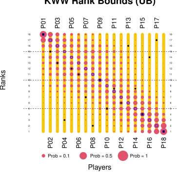
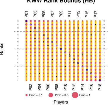
Figure 1: An alternative visualization of the Klein et al. (2020) 90% joint confidence region for overall ranking of baseball players with overlapping credible distributions for UB and HB models

By equation (9) of Klein et al. (2020) a $90\%$ joint confidence region for the rank vector $\check{r}$ is given by

$$\{(\check{r}_{1},\cdots,\check{r}_{18}):\check{r}_{k}\in\{1,2,\cdots,18\}\mbox{ for }k=1,\cdots,18\}.$$

This confidence set for the rank vector is depicted in Figure 1. Possible ranks for each player in this set are shown by a yellow line segment stretching from 1 to 18. According to this confidence set, any player can rank from 1 to 18, and any particular ranks can be held by any of these 18 players; clearly, it is totally uninformative. Due to multiple testing, the critical value $2.76$ (cf. equation (13) of Klein et al. (2020)) is too large to declare any comparison between two direct estimates to be significant. A joint $90\%$ credible distribution for the rank vector is a double-stochastic matrix, each row and each column of the matrix sums to one. This probability matrix is pictorially presented by overlaying on the figure of the confidence set solid red circles with area of a circle is proportional to the probability it is representing. The top matrix is based on the Cartesian credible set for $\theta$ under the unstructured Bayes model. From the figure, it is clear that many of the probabilities in this matrix are practically zeros implying that those combinations of players and ranks are improbable. Undoubtedly, the credible distribution is a lot more informative than the confidence set.

The observed rank $R_{i}$ of the $i$th player based on $y$ is shown by a blue square on the $R_{i}$th row and the $i$th column of the figure. If players $i_{1}$, $i_{2}$, $\cdots,i_{k}$ have the same $y$-values tied at ranks $r,r+1,\cdots,r+k-1$, we put $k$ blue squares on columns $i_{1}$, $i_{2}$, $\cdots,i_{k},$ of the $(r+k-1)$th row of this figure. [We followed the recommendation of Klein et al. (2020) to assign the highest possible rank to the tied players.] We used the remainder of the season performances of the players to compute their “true” rank vector $\xi$. The $i$th component, $\xi_{i}$, “true rank” for player $i$ is similarly depicted by a black circle on the $(\xi_{i},i)$ cell of the matrix.

The approach to the solution in the top panel of Figure 1 is the one which is the most similar to the Klein et al. (2020) solution. It is clear from the first row of this panel is that Player 1 has the largest probability of being the best hitter, and only the first five or six players have realistic chances to be the best hitter. Similarly, some of the players 12 through 18 are the most likely ones who had the lowest performance. These lists of players are much narrower than the whole set of $18$ players suggested by Klein et al. (2020) method. From the first column of this panel, on the other hand, we find that a realistic list of ranks for Player 1 is $\{14,15,16,17,18\}$. This list is much narrower than the entire set $\{1,2,\cdots,18\}$ suggested by the frequentist method. This figure also indicates that most likely ranks for player 17 are 1 to 7. The rank $17$ is most likely to be held by players 1 to 7. Clearly, the Bayesian solution is substantially more informative.

In the bottom panel of Figure 1 we depicted the double stochastic matrix from the HPD credible set for $\theta$ using the HB model. Due to shrinkage of the joint posterior distribution towards a vector of common means, probability distributions of the rankings of the few uppermost and the lowermost players are not as sharp as those provided by the corresponding credible distributions from the UB model. Even though there is a weakness of the HB method for its reliance on shrinkage to a common mean in the absence of a useful covariate, the method provides better solutions than the UB method for some players whose early batting averages are at odds with their latter scores. Here, five players (4, 8, 13, 16, 17) showed a large or moderately large discordance between their early and late season performances. Two most discordant players are 4 and 17. Player 4 did not perform well in the remainder of the season which earned him a very low surrogate rank $3$ compared to his high $y$ rank $15$. From the top panel of Figure 1 we see that whereas the UB method assigns, perhaps erroneously, nearly 87% probability of Player 4 having a rank higher than 9, the bottom panel of Figure 1 reveals that the HB method correctly assigns less than 63% probability to this player having such a high rank. At the other end, Player 17 performed very well in the remainder of the season which earned him a very high surrogate rank $17$ (vs. a very low $y$-rank 2). Here, again, Figure 1 for the unweighted UB Cartesian method assigns, perhaps erroneously, nearly 93% probability of it having a rank lower than 10, the bottom panel of Figure 1 for the HB method correctly assigns less than 67% probability to it having such a low rank. Revised rankings of the discordant players afforded by the HB method are noteworthy and more reliable. We have demonstrated through simulation in Subsection 7.1 and the median income example in Section 9 that the HB method in the presence of useful covariates is substantially more effective.

Also, for each player the variance of the possible ranks in the joint Klein et al. (2020) confidence region is $26.9$, the largest possible value, and the corresponding posterior variances from the credible distributions of ranks for these players vary between 5.36 and 16.36 for the UB model, and between 16.75 and 23.40 for the HB model. These numbers show a superiority of the credible distributions, created from the UB model or the HB model. We describe additional comparisons of the frequentist and the Bayesian solutions below.

Recall that $\xi_{i}$ is the rank of $\omega_{i}$, which is a surrogate or a “gold standard” value of $\theta_{i}$. We use these gold standard values $\xi_{i}$ of the ranks $\check{r}_{i}$ to assess accuracy of various credible distributions of overall rankings. In particular, we compute for player $i=1,\cdots,m,$

$$\epsilon_{i,HB,C} = E^{\pi_{{\check{r}}_{i},HB,C,y}}[|\check{r}_{i}-\xi_{i}||y],~{}\epsilon_{i,HB,E}=E^{\pi_{{\check{r}}_{i},HB,E,y}}[|\check{r}_{i}-\xi_{i}||y],$$

$$\epsilon_{i,UB,C} = E^{\pi_{{\check{r}}_{i},UB,C,y}}[|\check{r}_{i}-\xi_{i}||y],~{}\epsilon_{i,UB,E}=E^{\pi_{{\check{r}}_{i},UB,E,y}}[|\check{r}_{i}-\xi_{i}||y],$$

$$\epsilon_{i,KWW} = \frac{1}{|\Lambda_{Oi}|+1}\sum_{j=|\Lambda_{Li}|+1}^{|\Lambda_{Li}|+|\Lambda_{Oi}|+1}|j-\xi_{i}|,$$ (14)

where $\epsilon_{i,HB,C}$ is the posterior expectation of the absolute deviation of $\check{r}_{i}$ from $\xi_{i}$ with respect to the credible distribution $\pi_{{\check{r}}_{i},HB,C,y}$ from the HB model, and similarly, the other expectations. Finally, $\epsilon_{i,KWW}$ is the average of absolute deviations of $\xi_{i}$ from the possible values for $\check{r}_{i}$ given by the KWW confidence set $\{|\Lambda_{Li}|+1,\cdots,|\Lambda_{Li}|+|\Lambda_{Oi}|+1\}$ for $\check{r}_{i}$.

Table 1: Batting averages of 18 Major League players in 1970: $y_{i}$ is the average from first 45 at bats, $\omega_{i}$ the remainder of the season average, $R_{i}$ rank of $y_{i}$, $\xi_{i}$ rank of $\omega_{i}$, and deviation measures described in (14) for five overall ranking set estimators. For each of the two Bayesian models, we have two methods based on elliptical (subscript E) and Cartesian (subscript C) sets

Players	$y_{i}$	$\omega_{i}$	$R_{i}$	$\xi_{i}$	$\epsilon_{i,\small{HB,C}}$	$\epsilon_{i,HB,E}$	$\epsilon_{i,UB,C}$	$\epsilon_{i,UB,E}$	$\epsilon_{i,KWW}$
1. Clemente	.400	.346	18	18	5.90	5.90	1.18	1.18	8.50
2. F. Robinson	.378	.298	17	15	4.39	4.39	1.87	1.87	6.17
3. F. Howard	.356	.276	16	13	4.24	21.0	2.73	2.73	5.17
4. Johnstone	.333	.222	15	3	8.11	8.11	11.40	11.39	6.83
5. Berry	.311	.273	13.5	12	4.33	4.33	2.44	2.44	4.83
6. Spencer	.311	.270	13.5	11	4.25	4.25	2.96	2.96	4.61
7. Kessinger	.289	.263	12	7	4.96	4.96	4.92	4.92	4.83
8. L. Alvarado	.267	.210	11	2	7.66	7.66	8.13	8.13	7.61
9. Santo	.244	.269	9.5	10	4.36	4.34	3.09	3.09	4.50
10. Swoboda	.244	.230	9.5	5	5.41	5.41	3.98	3.98	5.61
11. Unser	.222	.264	6	8.5	4.26	4.26	3.09	3.08	4.56
12. Williams	.222	.256	6	6	4.40	4.40	2.64	2.64	5.17
13. Scott	.222	.303	6	16	7.64	7.64	9.36	9.36	6.83
14. Petrocelli	.222	.264	6	8.5	4.25	4.25	3.33	3.33	4.56
15. E. Rodriguez	.222	.226	6	4	5.38	5.38	3.46	3.46	6.17
16. Campenaris	.200	.285	3	14	6.64	6.64	8.97	8.97	5.61
17. Munson	.178	.316	2	17	9.54	9.54	13.57	13.56	7.61
18. Alvis	.156	.200	1	1	5.46	5.46	1.43	1.43	8.50
Total abs. dev.					101.16	101.16	88.56	88.56	107.64
$10^{13}\times$ Vol.					51.38	1.32	93756	1757	85722
Average length					0.236	0.193	0.359	0.288	0.357

From Table 1 we find that the Klein et al. (2020) method has the highest sum of average absolute deviations, about 6.4% larger than for the HB method, and about 21.5% larger than for the UB method. This is counter-intuitive as the shrinkage estimators of $\theta_{i}$’s from the exchangeable HB model have lower total squared error than the same for the direct estimators $Y_{i}$’s, which are Bayes estimates of $\theta_{i}$ under the UB model. We have noted above that the total squared error of UB estimate of $\theta$ from the “true” vector $\omega$ was $0.07537$, and for the HB estimate it was $0.02368$. We present below a possible explanation for the domination of the UB method over the HB method when it comes to inference for overall ranking based on their credible distributions.

In this example, estimating $\theta_{i}$ from the HB model shrinks the direct estimate; the shrinkage of $y_{i}$ towards a grand mean, measured roughly by the posterior mean of $E[D_{i}/(D_{i}+A)|y]$, is substantial (ranging between $0.75$ and $0.63$, and the shrinkage is more for the larger $D_{i}$’s that correspond to larger $y_{i}$’s. In our example, $D_{i}$’s decrease from $0.0053$ to $0.0029$, and the posterior mean of $A$ is $0.0024$ and the median of $A$ is $0.0017$.) These indicate that even in comparison with the small $D_{i}$’s, $A$ is small. In the absence of a covariate, a very small model error variance for an intercept only model essentially forces that $\theta_{i}$’s are all nearly equal. Accurate inference for the rank vector for such $\theta$ will naturally be challenging. Among the components of $\theta$, any differentiating information about $\theta_{i}$’s is given by its individual $y_{i}$’s only. Clearly, any shrinkage of an estimator of $\theta_{i}$ to a common value will reduce the estimator’s reliance on individual $y_{i}$’s, and thus the HB posterior distribution of $\theta_{i}$’s for ranking will be less informative than $y_{i}$, which is the center of the individual UB posterior distributions.

Due to lack of a covariate, corresponding to the set of larger observations (the first 4 or 5 observations which are in descending order), the HB posterior distribution of any of these $\theta_{i}$’s will shrink downward (to some grand mean). This downward shrinking of the posterior distribution of $\theta_{i}$’s will lower the probability of them holding the higher ranks (18 through 15 or 14). In fact, from Table 2 the posterior expectation of $\check{r}_{1}$ in our example is $12.1$, which is quite a bit smaller than the largest rank $18$ (in this case) it is supposedly estimating. Similarly, for the next two smaller observations, the posterior expected ranks are again quite smaller than the target ranks 17 and 16. These discrepancies contribute to a bigger absolute deviations reported in Table 1. On the other hand, the distributions of $\check{r}_{1},\check{r}_{2},\check{r}_{3}$ for the UB model do not shrink downward much since the posterior of $\theta_{i}$’s are independent and each is concentrated around its $y_{i}$. The corresponding posterior means of $\check{r}_{1},\check{r}_{2},\check{r}_{3}$ are $16.8,16.2$ and $15.2$ (cf. Table 2), which are not much smaller than $18,17$ and $16$, respectively. These lesser discrepancies make smaller contributions to the expected absolute deviations reported Table 1. A similar shrinkage upward will be noticed for the set of smaller observations (observations 14 through 18). Corresponding expected absolute deviations of the rank from the surrogate true rank $\xi_{i}$ for observations 14 through 18 under the HB model again tend to be bigger than their counterparts from the UB model. We see bigger discrepancies between the HB ranks and the UB ranks for the first 4 and the last 4 observations. All of these mostly explain the smaller total posterior expected absolute rank deviations for the UB model in comparison with their counterparts for the HB model.

Table 2: Estimation of ranks of baseball players by different methods

Players	P01	P02	P03	P04	P05	P06	P07	P08	P09
$y$ ranks	18	17	16	15	14	13	12	11	10
$\omega$ ranks	18	15	13	3	12	11	7	2	10
KWW	9.50	9.50	9.50	9.50	9.50	9.50	9.50	9.50	9.50
HB-Cart	12.10	11.86	11.60	10.94	10.41	10.94	10.27	9.57	9.35
HB-Ellip	12.10	11.86	11.60	10.94	10.41	10.94	10.27	9.57	9.35
UB-Cart	16.82	16.20	15.23	14.40	12.98	12.80	11.51	10.12	8.40
UB-Ellip	16.82	16.20	15.23	14.39	12.98	12.79	11.51	10.12	8.40
Players	P10	P11	P12	P13	P14	P15	P16	P17	P18	Average
$y$ ranks	9	8	7	6	5	4	3	2	1	9.5
$\omega$ ranks	5	8.5	6	16	8.5	4	14	17	1	9.5
KWW	9.50	9.50	9.50	9.50	9.50	9.50	9.50	9.50	9.50	9.5
HB-Cart	9.22	8.61	8.54	8.60	8.56	8.56	7.91	7.50	6.46	9.5
HB-Ellip	9.22	8.61	8.54	8.60	8.56	8.56	7.92	7.50	6.46	9.5
UB-Cart	8.41	6.71	6.69	6.64	6.43	6.79	5.03	3.43	2.43	9.5
UB-Ellip	8.41	6.72	6.69	6.64	6.43	6.79	5.03	3.44	2.43	9.5

Even though the UB method is poised to have smaller total expected absolute deviations than the HB method without a covariate, for some individual players the HB method is better suited to estimate ranks than the UB method. Continuing the above discussion further, since the posterior distribution of $\theta_{i}$ under the UB model is determined only by $y_{i}$, in case of a big discrepancy between $y_{i}$ and the unknown $\theta_{i}$ it is estimating (which will be reflected through a bigger difference between $y_{i}$ and $\omega_{i}$, the surrogate value of $\theta_{i}$), the posterior expected absolute deviation of $\check{r}_{i}$ from $\xi_{i}$ will be large ($\check{r}_{i}$, the rank of $\theta_{i}$, and $\xi_{i}$, the rank of gold standard value $\omega_{i}$). Indeed this happens for five players 4, 8, 13, 16 and 17 with large discordance between a player’s early and late season performances. Among these five players, player 17 has the second smallest observation, who displayed large discrepancies between $y_{i}$ and $\omega_{i}$. Deviations $\epsilon_{i,UB}$ for these players are much larger than the average deviations of the other players, and these deviations also exceed the corresponding players’ deviations $\epsilon_{i,HB}$ based on the exchangeable HB model. If one or more player substantially over-perform or under-perform in the remainder of the reason, based on their later performances the true ranks of these players will change substantially from their ranks determined by $y_{i}$’s. The HB method by virtue of its borrowing from the other players is better suited to rectify the erroneous ranks of the players based on $y_{i}$’s. This is the likely reason that the HB ranks for the five players identified above perform better than the UB ranks that are based on individual $y_{i}$ alone; a downward shrinkage of the HB posterior distribution of the over-performing (in their first 45 at bats) players 4 and 8, and an upward shrinkage of the HB posterior distributions of the under-performing (in their first 45 at bats) players 13, 16 and 17. The HB posterior distributions of $\theta_{i}$ of these players, by virtue of their borrowing information from the other players, are substantially pulled toward the “true value”, measured by $\omega_{i}$. This is a useful property of the HB model. No such borrowing of information is possible through the UB model as the posterior distributions of the components $\theta_{i}$’s are independent and centered around $y_{i}$.

Lastly, from this example where the total posterior expectation of absolute deviations of the true rank $\check{r}_{i}$ from the surrogate rank $\xi_{i}$ for the UB model is lower than the same for the HB model, we may not conclude that the UB model will always provide a more accurate solution. In fact, it is shown below by simulations that if a covariate effectively explains the $\theta_{i}$’s, the credible distributions of overall ranking based on the HB model are superior to the credible distributions derived from the UB model. Intuitively, this occurs since the posterior distribution of $\check{r}_{i}$ under the HB model will better concentrate near the true rank than the same posterior distribution under the UB model. We should note that even though in terms of total of expected absolute deviations, the frequentist Klein et al. (2020) method fares the worst, it is surprisingly robust for the five under-/over-performing players 4, 8, 13, 16 and 17. Finally, we included some size measures of the confidence set (for the KWW method) and credible sets for Bayesian methods, the sets are critical for the ranking problem. The last two rows of Table 1 provide volumes and approximate average lengths of the sets, respectively. In terms of volume, the HB sets are at least a thousand times better than the other sets. In terms of length, the HB sets are at least 50% better than the other sets. The best among all five sets is the HB elliptical set.

7.1 A simulation comparison of the set estimators of overall ranking

To run a simulation for a setup similar to the baseball example we generate 18 values of a covariate independently from a uniform (0,1) distribution. These covariates are kept fixed throughout the simulation. Using them, we generate $\theta_{i}$’s independently from $N(\beta_{0}+\beta_{1}x_{i},A)$. Using the generated $\theta_{i}$, we generate $Y_{i}$ from $N(\theta_{i},D_{i})$. We use the $D_{i}$ values from the baseball application. We use five possible values of $A=0.001,0.005,0.01,0.1$ and $1$ (for the baseball data estimate of $A$ is about $0.002$). We use $\beta_{1}=0$ (no covariate) and $\beta_{1}=0.4$. We use $\beta_{0}=0.2$, although $\beta_{0}$ does not influence the ranks and the results.

We report our simulation results in Table 3. First row of each block of the table, with a W in parentheses, reports average posterior expected deviations for weighted credible distribution, and the second row with UW in parentheses, shows results for its unweighted version. In the left half of these tables we presented results with a covariate and in the right half with no covariate. For each parameter setting, we provided the average of the mean absolute deviations of the overall ranks from the true ranks for KWW method, and average of the posterior expected absolute deviations for Bayesian methods: HB and UB. We also presented average volumes and average of lengths of the sides of various 90% confidence or credible sets of the true mean vector $\theta$.

When we compare in terms of size measures, the $m$th root of the volume (to avoid dealing with very large or very small numbers, we consider the $m$th root) and the average length of the confidence or credible sets of $\theta$, the HB elliptical credible set performed the best. In terms of the average posterior expected deviations of ranks from their true values, the performance of the HB solution is mixed and the Klein et al. (2020) method has the weakest performance. Smaller values of $A$ (0.001, 0.005, 0.01), relative to the $D_{i}$’s, introduce a lot of structure to the $\theta_{i}$’s. In these cases in the absence of any covariate, $\theta_{i}$’s tend to be a lot similar, where the UB method performs better based on deviation criterion. However, when the $\theta_{i}$’s vary according to a covariate, the HB method performs substantially better for smaller values of $A$. For larger values of $A$, $0.1$ and $1$, even with the covariate, $\theta_{i}$’s do not display much of any structure (relative to the $D_{i}$’s, $A=0.1$ is between 19 and 35 times the $D_{i}$’s, and $A=1$ is between 190 and 350 times larger). The case of $A=1$ relative to the $D_{i}$’s is similar to our next example where we develop ranking of the US states based on average commuting times. For the last two cases of $A$, the HB posterior distribution of $\theta$ will have negligible shrinkage and it is approximately equal to unstructured Bayesian posterior distribution, resulting in similar inference for credible distribution of overall ranking; the UB method is marginally better than the HB method in terms of the deviation measure. Finally, in terms of this measure, the overall ranking for the elliptical method does better than the Cartesian method when the double stochastic matrix is created by unweighted method. However, when the credible distribution is created by weighted method, the credible distributions from elliptical and the Cartesian sets perform very similarly.

Table 3: Summary of simulations for the baseball setup

		With covariate					Without covariate
			H. Bayes		U. Bayes			H. Bayes		U. Bayes
$A$		KWW	Cart	Ellip	Cart	Ellip	KWW	Cart	Ellip	Cart	Ellip
	Ave Post Exp Abs Dev (W)	5.518	1.178	1.178	2.313	2.313	5.978	5.366	5.366	4.642	4.642
	Ave Post Exp Abs Dev (UW)	5.518	1.543	1.521	2.560	2.545	5.978	5.194	5.199	4.804	4.795
0.001	(Ave Volumes)1/m	0.356	0.262	0.212	0.357	0.286	0.356	0.259	0.209	0.357	0.287
	Ave length of the sides	0.357	0.247	0.199	0.358	0.287	0.357	0.241	0.196	0.358	0.287
	Ave Post Exp Abs Dev (W)	5.268	1.835	1.835	2.148	2.148	5.919	4.065	4.066	3.468	3.468
	Ave Post Exp Abs Dev (UW)	5.268	2.033	2.020	2.378	2.365	5.919	4.094	4.094	3.714	3.701
0.005	(Ave Volumes)1/m	0.356	0.297	0.238	0.357	0.287	0.356	0.295	0.237	0.356	0.286
	Ave length of the sides	0.357	0.289	0.232	0.358	0.287	0.357	0.281	0.227	0.358	0.287
	Ave Post Exp Abs Dev (W)	4.879	1.874	1.874	1.980	1.980	5.668	2.967	2.967	2.766	2.766
	Ave Post Exp Abs Dev (UW)	4.879	2.063	2.053	2.188	2.176	5.668	3.211	3.203	3.013	2.999
0.010	(Ave Volumes)1/m	0.356	0.318	0.255	0.357	0.286	0.356	0.317	0.254	0.357	0.287
	Ave length of the sides	0.357	0.314	0.252	0.358	0.287	0.357	0.312	0.251	0.358	0.288
	Ave Post Exp Abs Dev (W)	2.919	1.070	1.070	1.061	1.061	3.212	1.177	1.177	1.168	1.168
	Ave Post Exp Abs Dev (UW)	2.919	1.205	1.198	1.194	1.186	3.212	1.328	1.319	1.313	1.305
0.100	(Ave Volumes)1/m	0.356	0.351	0.282	0.356	0.287	0.356	0.350	0.281	0.356	0.286
	Ave length of the sides	0.357	0.352	0.283	0.358	0.287	0.357	0.351	0.282	0.358	0.287
	Ave Post Exp Abs Dev (W)	1.209	0.417	0.417	0.418	0.418	1.181	0.370	0.370	0.369	0.369
	Ave Post Exp Abs Dev (UW)	1.209	0.467	0.465	0.467	0.464	1.181	0.426	0.423	0.426	0.423
1.000	(Ave Volumes)1/m	0.356	0.356	0.286	0.357	0.287	0.356	0.356	0.286	0.357	0.287
	Ave length of the sides	0.357	0.357	0.287	0.358	0.288	0.357	0.357	0.287	0.358	0.288

8 Ranking of the US states based on commuting times

In a pioneering article, Klein et al. (2020) applied their frequentist approach to rank fifty states of the U.S. and DC by mean commuting times of workers sixteen or older and not working from home. They used survey data collected from the ACS. In Figure 2 below, we recreated Figure 1 of Klein et al. (2020) that depicted the frequentist solution of the confidence region for ranking from equation (8). Possible ranks for state $i$ in this set are shown by a pink line segment stretching from $|\Lambda_{Li}|+1$ to $|\Lambda_{Li}|+|\Lambda_{Oi}|+1$. From the figure, for example, the possible ranks from this solution for the state ID are $4-9$. On the other hand, the states which can hold the rank 9 are the states WY, AK, MT, IA, KS and ID (the pink line segments for these states intersect the horizontal line for ranks = 9). The rank based on direct estimate $y_{i}$ is shown by a black dot at its rank $r$. If two states tie for ranks $r,r+1$, their tied ranks are shown by a line segment joining these states at rank $r+1$. For example, SD and ND direct estimates tie for ranks 1 and 2. We showed this by the black line joining the two states.

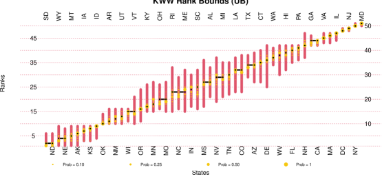
Figure 2: An alternative visualization of the 90% joint confidence region for travel time ranking given by Figure 1 of Klein et al. (2020) with an overlapping credible distribution from unstructured Bayes method

On Figure 2 we overlaid the credible distribution based on a Cartesian credible set from the unstructured Bayes model. Both in terms of the model and the method, this table is most directly comparable with Figure 1 of Klein et al. (2020). Probabilities from credible distribution are shown by yellow circles, bigger circles for larger probabilities. To clearly interpret the probabilities depicted in the figure, let us focus specifically on its $4$th row and $4$th column. From the $4$th column of this figure we find that the state of NE can have ranks 3-6 with respective probabilities about $0.2,0.2,0.5,0.1$ (actual values are $0.21,0.20,0.55,0.04$). We can contrast this with the red band on the 4th column in the figure which shows the rank set for NE suggested by the Klein et al. (2020) solution. It shows that in addition to the four ranks 3-6, NE can also rank 1, 2, 7 and 8. On the other hand, the fourth row of the figure corresponding to rank 4 shows that the states that can plausibly hold this rank are AK, MT, NE and WY with respective probabilities about $0.05,0.2,0.5,0.2$ (actual values are $0.04,0.23,0.55$ and $0.18$). Again, in contrast, the 4th row in Figure 1 of Klein et al. (2020) shows that states SD, ND, WY, NE, MT, AK, IA, KS and ID are all contenders of rank 4. Compared to the Bayesian solution, the frequentist solution includes five additional states. From all the posterior samples of the vector $\theta$ (not only those that are included in the credible set), in Figure 3 we created the scatter plot of NE vs. IA, using their components from $\theta$. The entire scatter plot is practically below the line $y=x$, implying that it is improbable for IA and NE to hold the same rank.

As another example, if we consider ID, we find from our table that it can hold only rank 9, and the rank 9 can only be held by Idaho. On the other hand, we observed it earlier that for the frequentist solution possible ranks for ID are 4-9, and the states that can rank 9th are WY, MT, AK, IA, KS and ID. Similarly, while SD and ND, tied by direct estimates, and both have the same frequentist rank set $1-6$, according to credible distribution ranks, only possible ranks for these states by the credible distribution are $1$ and $2$, and SD has $60\%$ probability to hold rank $1$ (note that SD direct estimate has a smaller standard error). Clearly, all these results demonstrate that our Bayesian results are “less dispersed”, “more illuminating” and “more conclusive”.

Figure 3: Scatter plot of the posterior samples of commuting times for IA and NE

We also compute the credible distribution (i.e., the double stochastic matrix), not shown here, based on the elliptical region from the HB model. From the $4$th row of this matrix we find that the states AK, MT, NE and WY are the contenders of rank 4, and they may hold this rank with probabilities $0.11,0.21,0.50$ and $0.18$, respectively. The fourth column of that matrix conveys that NE can hold the ranks 3, 4, 5 and 6 with probabilities $0.32,0.50,0.15$ and $0.04$, respectively. Close agreements between these probabilities and those for the other cases show that credible regions of $\theta$ having different shapes and derived from different models provide reasonably similar solutions for overall ranking. We have no covariate for this example and the HB estimate of the model error variance $A$ is $13.2$, which is about $56$ times the largest sampling variance $D_{i}$ and $3572$ times the smallest one. With so high ratios of the model variance to sampling variances, the HB model is practically identical to the UB model. Similar credible distributions from the UB and the HB models in this application are confirmed by the simulation study we presented in Table 3. From the two lower-right-bottom blocks of this table, we find the average posterior mean absolute deviations reported for the UB and the HB columns show no practical differences among the four Bayesian solutions (2 models times 2 shapes). In the last block we set $A=1$ which is nearly $188$ times the largest sampling variance and $342$ times the smallest one.

We also compare all five confidence and credible regions of $\theta$ in terms of their size measures. From Table 4 we find that all four Bayesian credible sets have smaller volumes than the KWW confidence set. While volumes of Cartesian credible sets are between $31\%$ and $38\%$ smaller than the volume of the KWW set, the elliptical shape HPD credible sets are enormously superior (by an order of $10^{-7}$) to the other set estimators with hyperrectangular shapes (this is due to cutting off low probability “corners” of the hyperrectangular sets to create an HPD set). Even in terms of average length, elliptical-shaped sets are better than the hyperrectangular-shaped sets. Finally, with no surprise to us, we observe that in terms of these size measures credible sets from the HB model are better than the credible sets from the unstructured Bayes model.

Table 4: Commuting time: Comparison of size of set estimators of $\theta$, frequentist and Bayes.

	Frequentist	Unstructured Bayes		Hierarchical Bayes
Measure	KWW	Cartesian	Elliptical	Cartesian	Elliptical
Volume	4.52	3.54	$1.89\times 10^{-7}$	3.42	$1.46\times 10^{-7}$
Ave length	1.16	1.16	0.83	1.15	0.83

9 Ranking of the US states based on median incomes

Inference on median incomes of the US states for the income year 1989 has served as a benchmark example to evaluate effectiveness of various small area estimation methods. See for example, Ghosh et al. (1996) and Chung and Datta (2022). For this application, these researchers suggested various innovative small area estimation methods to estimate the true four-person family median incomes ($\theta_{i}$) for the fifty US states and Washington, DC. They used survey data from the Current Population Survey (CPS) that provides annual estimates of median incomes for the states for various family sizes. These estimates serve as the direct estimates for the popular Fay-Herriot model. The application enables borrowing strength from other covariates by integrating administrative data and the past census data. For this application Fay (1987) suggested in addition to the intercept using two covariates in the Fay-Herriot model in Section 2.2. The first covariate $x_{i1}$ is the $i$th state median income for 1979 from the preceding Census in 1980. The second covariate, $x_{i2}$, is an adjusted version of $x_{i1}$. The adjusted Census median income $x_{i2}$ for the $i$th state is given by $x_{i2}=(\text{PCI}_{i,1989}/\text{PCI}_{i,1979})x_{i1}$, $i=1,\ldots,m$, where $\text{PCI}_{i,1979}$ and $\text{PCI}_{i,1989}$ are the 1979 and 1989 per capita incomes of the $i$th state provided by the Bureau of Economic Analysis of the U.S. Department of Commerce. Small area estimates using these covariates have been effectively compared with the corresponding incomes obtained from the 1990 Census that collected data for the 1989 income year. The census incomes for the states were medians based on a large number of households from each state. Due to large sample sizes the state census median incomes are treated as “gold standards” and are believed to be effective “surrogates” for the true 1989 state median incomes, $\theta_{i}$, which we are trying to rank.

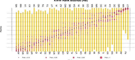
Figure 4: A visualization of the 90% joint confidence region for median income ranking by Klein et al. (2020) with an overlapping credible distribution from the hierarchical Bayes method

In Figure 4, we recreated for our application Figure 1 of Klein et al. (2020) that depicted the frequentist solution of the confidence region for ranking from equation (8). On this figure we overlaid the credible distribution based on the weighted HB model. The KWW rank sets for all the states are depicted by appropriate yellow line segments that span a subset of 1 to 51. Probabilities from credible distribution are shown by red circles, bigger circles for larger probabilities. We use solid black circles on this figure to depict the “true” states ranks based on their median incomes from the 1990 census by. For our application, the frequentist KWW solution assigns ranks 1 to 46 to the state MS; it is hardly informative. The HB credible distribution assigns probabilities $0.25,0.11,0.14,0.14,0.06,$ and $0.20$ to the ranks 1 to 6. Rest of the ranks have negligible probabilities, adding up to $0.1$. To the state CT the KWW solution assigns ranks 15 to 51, which is again very wide. The HB Cartesian credible distribution assigns probabilities $0.03,0.13,0.33,$ and $0.51$ to the ranks 48 to 51. Clearly, the Bayesian solution is very compact. For NJ, the KWW ranks span from 22 to 51. The HB solution assigns probabilities $0.04,0.53,$ and $0.43$ to the ranks 49-51. The Bayesian solution is vastly superior to the frequentist solution.

Table 5: Median incomes: Comparison of set estimators of $\theta$, frequentist and Bayes, by size measures, and comparison of overall ranking methods by total average absolute deviations from gold standard ranks. For each of the two Bayesian models, we have two methods based on elliptical (subscript E) and Cartesian (subscript C) sets. All volume measure have been scaled by a known constant $g$ and all length measures have been scaled by a known constant $h$.

Measures	$\epsilon_{i,\small{HB,C}}$	$\epsilon_{i,HB,E}$	$\epsilon_{i,UB,C}$	$\epsilon_{i,UB,E}$	$\epsilon_{i,KWW}$
Total abs. dev.	179.52	179.52	388.11	388.11	798.66
Volume/$g$	$4.619\times 10^{19}$	$2.975\times 10^{12}$	$8.321\times 10^{26}$	$4.043\times 10^{19}$	$1.080\times 10^{27}$
Ave length/$h$	2.478	1.785	3.569	2.567	3.589

Table 6: Average or expected absolute deviations for the Income Data

KWW HB-Ellip UB-Ellip MS 22.50 2.87 5.76 AR 22.54 2.63 8.45 NM 20.13 1.97 2.05 WV 19.76 1.63 3.25 LA 20.41 5.95 12.65 SD 18.64 2.78 3.67 KY 18.38 3.50 3.95 MT 15.77 3.30 4.92 OK 18.41 4.70 19.75 ID 15.91 2.91 3.44 ND 16.24 3.42 7.38 AL 15.25 2.66 5.96 TN 14.32 3.08 7.13 SC 14.29 2.21 6.16 TX 12.27 3.47 6.31 NE 14.71 5.52 13.00 UT 13.94 2.58 6.09 WY 14.00 6.13 6.79 IA 12.98 3.30 4.64 NC 12.42 2.68 2.23 AZ 13.24 4.03 9.30 OR 13.06 3.85 9.33 MO 12.92 4.05 7.57 KS 12.82 4.93 11.83 ME 12.50 4.97 5.82 FL 12.04 3.60 7.10

KWW HB-Ellip UB-Ellip GA 12.76 4.98 15.00 VT 12.82 3.80 6.51 IN 12.92 3.43 5.33 OH 12.12 5.70 10.69 WI 13.24 3.27 5.05 PA 13.24 3.31 4.15 CO 13.55 5.08 14.80 NV 13.90 5.09 21.42 WA 14.33 2.91 5.48 MI 13.90 3.89 3.29 MN 15.12 3.44 5.53 VA 15.57 5.54 8.41 DC 16.06 5.99 17.91 IL 16.70 2.17 5.43 RI 17.16 3.09 4.06 NY 15.60 1.76 4.40 CA 18.86 4.96 12.82 NH 15.30 2.39 4.04 DE 19.82 9.29 18.55 HI 20.59 3.05 7.57 MD 21.39 0.99 3.48 AK 22.24 1.28 15.31 MA 10.73 0.45 1.48 NJ 13.57 0.47 1.61 CT 18.00 0.68 1.22 Average 15.67 3.52 7.61

We compare the frequentist and four Bayesian sets for $\theta$ by using their volume and length measures. We present these results in Table 5. Volumes of Bayesian sets are vastly smaller than the frequentist confidence sets. The HB elliptical set has the smallest volume. Average lengths of Bayesian sets are smaller than the average length of confidence set, again the HB elliptical set has the smallest average length. Here each of the volume numbers are scaled by a known constant $g$, and each of the length numbers are scaled by a known constant $h$.

In Table 6 we presented for each state average absolute deviations (cf. equation (14)) of the KWW ranks from the surrogate ranks based on 1989 income data from the census. We also presented the posterior expected absolute deviations, obtained from (14), for the credible solutions. The deviations for KWW method exceed the deviations for the HB method for all $51$ states, and those exceed $46$ deviations for the UB method excluding OK, GA, CO, NV, and DC. We find that the KWW method has the highest sum of average absolute deviations (799), about 344% larger than for the HB method, and about 116% larger than for the UB method. Clearly, the HB method is the best.

For the median income application we further explore comparison of credible distributions generated by various Bayesian models (UB and HB, with and without covariates) and methods (weighted and unweighted) among themselves and with the frequentist method of KWW in terms of average absolute deviations and posterior expected absolute deviations defined in equation (14). We plotted several of these posterior expected absolute deviations against the KWW average absolute deviations in Figure 5.

The left panel in the first row of Figure 5 is the plot using posterior expected absolute deviations from credible distributions from weighted method based on the HB model with covariates on the $y$-axis and the KWW deviations on the $x$-axis. On this plot we use the green circles for the elliptical method and the black stars for the rectangular method. This panel shows that all the points cluster below the $y=x$ line and closer to the $x$-axis, indicating that the credible distributions are vastly superior to the KWW method. It also shows that for the weighted method there are practically no differences between the deviations from credible distributions based on the rectangular or the elliptical credible sets for the mean vector $\theta$.

The right panel in the first row of that figure differs from the left panel only by use of no covariates in the HB model. We see that several points are above the $y=x$ line, indicating that the KWW solution for those states are better than the HB solution in the absence of covariates. Also, although many of these points that are below the $y=x$ line, a large number of points are above the line $y=5$ in contrast with the left panel where only about $15\%$ of the points are above the $y=5$ line, indicating that the credible distributions in the absence of good covariates are not as good as those created by using good covariates. These two panels convincingly demonstrate the importance of effective covariates for the ranking problem.

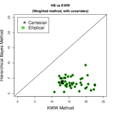
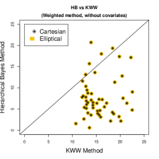
Figure 5: Various plots of expected or average absolute deviations

With Covariates	Covariates not used
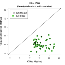
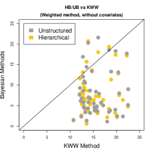
With Covariates	No covariates, elliptical
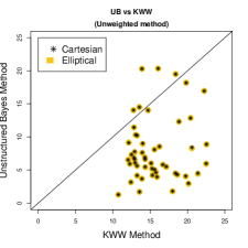
Covariates cannot be used	Covariates cannot be used

The left panel on the second row mimics the left panel on the first row except that now the credible distributions are unweighted. The HB model employs covariates. As we have noticed in the first row, in this case also we see that the Bayesian solutions (both elliptical and rectangular) are vastly better than the KWW solution. However, while most of the points on the panel in the second row are above the line $y=5$, most are below that line in the panel on the first row. These two panels show the superiority of the weighted credible distributions. In the right panel on this row we plotted the deviations based on weighted, elliptical credible distributions for the UB model and the HB model without covariates against the KWW deviations. While overall the credible distributions show superiority over the KWW method, for about $10\%$ of the states the KWW method performed better. None of these methods utilized any covariates. This plot also shows that in the absence of a covariate the HB method loses its advantage over the UB method, the two credible distributions performed rather similarly.

In the last row of the figure, we compare various credible distributions (weighted vs. unweighted, elliptical vs. Cartesian) from the UB model against the confidence set provided by the KWW method in terms of posterior expected absolute deviations (resulting from the credible distributions) and average absolute deviations (resulting from the KWW method). While again the UB credible distributions show overall superiority over the KWW method, for about $10\%$ of the states the KWW method performed better. None of these methods utilized any covariates.

10 Summary and Conclusions

Inference for population means (or proportions) of subpopulations or subjects, is an important statistical problem. In survey sampling estimation of small area characteristics, in animal science and livestock research estimation of breeding values of various herds, in sports estimation of true performance of various players, and in healthcare estimation of treatment effectiveness for certain conditions treated by several health facilities, are some of the important problems in multi-population studies. The major focus in statistical inference for multiple populations has been estimation (point and interval) of means or proportions or similar measures from several subpopulations or individuals. In small area estimation where the main goal has been estimation of small area means, the companion problem of simultaneously estimating the ranks of the small areas is also of considerable importance but it has not gotten enough attention. Only Shen and Louis (1998) simultaneously considered estimation of small area means and ranks. Using the HB approach these authors considered point estimation of ranks but did not account for error in estimation of the rank vector for all small areas.

To account for estimation error for the rank vector of many subpopulations, in a pioneering article Klein et al. (2020) considered set estimation of overall ranking. Klein et al. (2020) created joint confidence set of the rank vector by employing a rectangular confidence set of the mean vector $\theta$. Their solution in equation (8) attributes $|\Lambda_{Li}|+1,\cdots,|\Lambda_{Li}|+|\Lambda_{Oi}|+1|$ as the possible values for the true rank ${\check{r}}_{i},i=1,\cdots,m.$ This solution, frequentist by construction, may be interpreted as a confidence distribution for ${\check{r}}_{i}$, uniformly distributed over the integers between the lower and the upper bounds presented above. As an alternative to this method, which cannot use auxiliary information or model the unknown true mean $\theta$, we introduced a Bayesian model for the mean vector. The model allows us to utilize useful auxiliary information as well as to develop various credible sets for $\theta$ including the HPD sets that are exact or nearly exact. We create a credible distribution for the true rank ${\check{r}}_{i}$, which is more informative than the confidence set by KWW. In our Bayesian proposal we can also allow more probable $\theta$’s in the credible set to have them bigger weights to the credible distribution.

Application of proposed credible distributions is computationally straightforward. We applied our solution to three applications, one to rank professional baseball players, and two to rank small areas based on unknown small area means. All three applications and a simulation study mimicking two of the applications demonstrated superior performance of the proposed method over the existing frequentist method. For the baseball example there are no reliable covariates but there are surrogate values of the true means from the players’ performance from the remainder of the season. Evaluation of frequentist confidence set and the credible distributions based on the average or expected absolute deviations of estimated ranks from the ranks of the surrogate values show better performance for the Bayesian solutions. In the absence of covariates, the UB credible distribution performs better than the HB credible distribution. For the commuting time example we neither have any covariates nor any representative values of the unknown true means. Even then in this example the credible distributions are “more conclusive”, “less dispersed” and “more illuminating” than the frequentist solution by Klein et al. (2020). For the median income estimation problem we have useful covariates as well as representative values (from the 1990 census) of the true means. Credible distributions from the HB model with the covariates performed the best when measured in terms average absolute deviations. Both credible distributions, from the UB model and the HB model, have better performance than the frequentist method. The HB credible distribution based on covariates is uniformly better than the other two solutions. However, the HB credible distribution without any covariates does not enjoy a uniform superiority over the other two solutions. These outcomes are confirmed by our simulation study for the setup of the baseball application. Availability of good covariates show the superiority of the HB credible distribution. Lack of covariates degrades the performance of the HB credible distribution, which is sometimes inferior to the UB credible distribution. In terms of size measures of the confidence or credible sets, the Bayesian solutions are vastly superior, and between the two Bayesian solutions, the HB-based credible sets are shorter or more “compact” than the UB-based credible sets.

Disclosure Statement

There are no competing interests to declare from the authors.

Funding

This work was partially supported by the National Science Foundation (NSF) grant DMS-2311186.

Appendix: size measures of elliptical sets

As an alternative to an orthotope (or hyperrectangular) credible set, where each component of $\theta$ varies freely, we have considered HPD sets which are approximately elliptical for our Bayesian models. Two size measures that appear to be appropriate for set estimators are their Lebesgue volumes and average lengths of the “sides” determining the set. These two measures are easily found for an orthotope. We compute representative values of these size measures of the elliptical sets.

To determine reasonable size measures for elliptical regions, we proceed with an ellipse defined by

$$E=\{x:x^{T}Kx\leq c\},$$ (15)

where $K$ is an $m\times m$, p.d. matrix, and $c>0$. Since the center of the ellipse has no role in the size measures, we take it zero. Let $V_{E}(K,m,c)$ denote the Lebesgue volume of the set $E$. It can be easily calculated that

$$V_{E}(K,m,c)=\frac{\pi^{m/2}}{\Gamma((m+2)/2)}\times\frac{c^{m/2}}{\mbox{det}(K)^{1/2}},$$ (16)

where $\Gamma(\cdot)$ is the gamma function and $\mbox{det}(K)$ is the determinant of $K$.

A standard length measure of an elliptical region is not available. We derive below a reasonable expression for it. For an $m$-dimensional rectangular region, its volume is the product of the volume of the $(m-1)$-dimensional of the cross-section of the set defined by the intersecting hyperplane, say, $\theta_{1}=d$, and the length $(U_{1}-L_{1})$ of original rectangular set along the $\theta_{1}$ direction (where $L_{1}<d<U_{1}$). Thus, the length of the set along the $x_{1}$ direction is the ratio of the volume of the original orthotope to the volume of the lower-dimensional cross-section orthotope.

We will use the above discussion for the orthotope region as an analogy to come up with a suitable “length” for the ellipse along the $x_{1}$ direction. For the ellipse, we take for any $x_{1}$ and $x_{(2)}=(x_{2},\cdots,x_{m})^{T}$ with $(x_{1},x_{(2)}^{T})^{T}$ inside the set, we define a central cross-section by the hyperplane $x_{1}=-K_{12}x_{(2)}/K_{11}$, where we partition the matrix $K$ as $((K_{ij}))$, $i,j=1,2$, in conformity with the partitioning of $x$ above. We also define the p.d. matrix $K_{22.1}=K_{22}-K_{21}K_{11}^{-1}K_{12}$. The corresponding cross-section is $E_{C}=\{x_{(2)}^{T}K_{22.1}x_{(2)}\leq c\}.$ From equation (16), it similarly follows that

$$V_{E_{C}}(K_{22.1},m-1,c)=\frac{\pi^{(m-1)/2}}{\Gamma((m+1)/2)}\times\frac{c^{(m-1)/2}}{\mbox{det}(K_{22.1})^{1/2}}.$$ (17)

A reasonably representative length for the $x_{1}$ side of the ellipse is the ratio of the volume in (16) to the volume in (17). Simplification leads to an expression. From this, after simplification, in general, we have along the $x_{i}$ direction the representative length, $L_{R,i}$ (say), is

$$L_{R,i}=B(\frac{1}{2},\frac{m+1}{2})\times\{\sqrt{c}/\sqrt{K_{ii}}\},~{}i=1,\cdots,m,$$ (18)

where $B(a,b)$ is the regular beta function.

The above proposal of the length of a side of an elliptical region is only heuristic. Indeed it is a reasonable requirement that these lengths should be “calibrated” by a suitable scale so that for the modified orthotope based on the lengths of the “scaled sides” will match the volume of the original ellipse. Based on this consideration, the modified lengths $L_{M,i}$ are given by

$$L_{M,i}=\{V_{E}(K,m,c)/\prod_{i=1}^{m}L_{R,i}\}^{1/m}L_{R,i}.$$ (19)

Mean of the $L_{M,i}$’s is a “linear” measure, $L_{E}$, of the elliptical set, and may be compared to $L_{C}$.