A Wild Bootstrap Procedure for the Identification of Optimal Groups in Singular Spectrum Analysis

Abstract

A key step in separating signal from noise using Singular Spectrum Analysis (SSA) is grouping, which is often done subjectively. In this article a method which enables the identification of statistically significant groups for the grouping step in SSA is presented. The proposed procedure provides a more objective and reliable approach for separating noise from the main signal in SSA. We utilize the $w$-correlation and test if it close or equal to zero. A wild bootstrap approach is used to determine the distribution of the $w$-correlation. To identify an ideal number of groupings which leads to almost perfect separation of the noise and signal, a given number of groups are tested, necessitating accounting for multiplicity. The effectiveness of our method in identifying the best group is demonstrated through a simulation study, furthermore, we have applied the approach to real world data in the context of neuroimaging. This research provides a valuable contribution to the field of SSA and offers important insights into the statistical properties of the $w$-correlation distribution. The results obtained from the simulation studies and analysis of real-world data demonstrate the effectiveness of the proposed approach in identifying the best groupings for SSA.

MSC Classification]94A12, 62F40, 62J15

Declarations]The authors have no competing interests to declare that are relevant to the content of this article. Friederike Preusse gratefully acknowledges funding by the Deutsche Forschungsgemeinschaft (DFG, German Research Foundation)- project number 281474342. Anna Vesely acknowledges partial financial support by the Deutsche Forschungsgemeinschaft (DFG) via Grant No. DI 1723/5-3.

Authors Contribution] MM and AV developed the methodology, DO programmed the SSA part of the simulation and wrote the introduction. AV and FP implemented the methodology and wrote the respective sections. Simulations were performed by MM, application to real-world data was done by FP. TD recommended the usage of the wild bootstrap, and he searched for relevant literature. All authors proofread and approved the final manuscript.

1 Introduction

There is a common mantra among the practitioners especially those from the frequentist school of thought that “One should let the data speak for themselves”. More often than not, this data set comes with some noise in it, so pre-processing data is an essential step for data analysis. In this regard, noise reduction and signal extraction have always been considered as an important step of data analysis in all fields of study; see, among many others, [Pyle1999, Repsilber2008, OLIVERI20199, Maryam2]. There are two main approaches for analyzing noisy time series. According to the first approach, we can ignore the presence of noise and analyze the data the way it is. Of course this can lead to wrong conclusions due to the noise. According to the second approach, we can filter the noisy time series to reduce the noise level and then analyze the new data points.

Singular Spectrum Analysis (SSA) is a non-parametric denoising method for analyzing one or even multi-dimensional time series. This procedure is widely used since it covers a wide range of application areas, including those related to ecological and environmental data, medicine, economic, and financial time series (see for example [ex1, ex2, ex3, ex4, ex5, ex6, ex7, ex8, ex9] and references therein). A detailed description of other popular denoising methods for one dimensional time series data are summarized in a report by [kohler2005comparison]. In the SSA method, the observed time series (signal+noise) is transformed into a matrix of overlapping consecutive sub-signals, which is called the trajectory matrix, and because of this transformation, SSA is an especially helpful technique in dealing with small sample sizes. By overlapping sub-signals together it can be possible to have a suitable view of the inter-dependency of the data. The key step in SSA is grouping, which involves separating noise from the main signal in the time series data.

Traditional approaches for grouping in SSA are often subjective and can lead to inconsistent results. These approaches typically involve selecting a group size based on expert knowledge or heuristic rules. However, this subjective approach can lead to different results depending on the analyst’s experience or the specific problem at hand. To overcome this limitation, in this paper we propose a new method for identifying the statistically best group to separate noise from the main signal in SSA using a wild bootstrap method. Bootstrap procedures are a powerful non-parametric statistical technique that can be used to estimate the sampling distribution of a statistic when the underlying distribution is unknown. The proposed method involves using the bootstrap procedure proposed in [hounyo2023wild] to find the distribution of $w$-correlation, which can then be used to determine the optimal grouping for SSA. This bootstrap procedure is preferred since, just like the SSA methodology, it does not require the restrictive assumption of stationary time series. Furthermore, it works for both dependent and heterogeneous data which are common in time series and therefore - again - we are not restricted to the i.i.d. (independent and identically distributed) set up. The approach presented in this paper represents a significant advance in the field, as it is the first time that researchers can identify the best group statistically. By using the proposed method, data analysts and researchers can achieve more objective and reliable grouping in SSA, which can lead to more accurate results.

1.1 Related work

The moving block bootsrap (MBB) is an extension of Efron’s i.i.d. bootstrap to dependent data and was independently introduced by Künsch (1989) and Liu and Singh (1992). The MBB has since been an active area of research in time series since it can be used to calculate the unknown sampling distribution of complicated statistics. Furthermore, it can be used for a large class of heterogeneous weakly dependent time series and just like any other bootstrap procedure, provides better approximations to the distribution of a statistic compared to those based on asymptotic normality. The MBB samples overlapping blocks with replacement which are then joined together to form a bootstrap sample. Some of the most common versions of the MBB include the dependent wild bootstrap (DWB) [shao2010dependent] applicable to stationary, weakly dependent data, the circular block bootstrap (CBB) [politis1991circular], the matched block bootstrap [carlstein1998matched], the nonoverlapping block bootstrap (NBB) [carlstein1986use], the stationary bootstrap (SB) [politis1994stationary], and the tapered block bootstrap (TBB) [paparoditis2001tapered], among others. A wild bootstrap for dependent data (WBDD) that makes use of external random variables and that can be used to calculate standard errors of estimators and confidence regions for parameters when dealing with dependent and heterogeneous data was considered by [hounyo2023wild]. With an appropriate choice of the external random variable, the WBDD procedure preserves the second-order correctness property of blockwise bootstrap for smooth functions of the mean. Also, the WBDD generalizes the DWB since these external random variables do not have to be from a stationary process.

1.2 Main contributions

The weighted correlation coefficient, or $w$-correlation, is a useful measure that can be used in judging how well the signal and noise have been separated in SSA. A value close to zero is an indication that the number of groups used are sufficient and hence the noise and signal are well separated. To enable us to identify the ideal number of groups in the grouping step of the SSA, we conduct inference on the weighted correlation coefficient utilizing the wild bootstrap procedure proposed by [hounyo2023wild]. This procedure allows us to calculate the intractable sampling distribution of the $w$-correlation in a simple manner and therefore we are able to calculate the test statistic and $p$-values used in our inference. Unlike the blockwise bootstrap methods which resamples blocks of observations to form a bootstrap sample, the wild block bootstrap uses external random variables which are independent of the data to weigh the data to capture the dependence nonparametrically. Given that we are dealing with non-stationary time series data, we require a more general version of the mixing assumption called near epoch dependent (NED) which can also allow for heterogeneity. Since we have to test all the possible groupings $g\in\{1,2,\ldots,d\}$, this leads to a multiple testing problem with the possible number of groups as the source of the multiplicity. Moreover, since the number of groupings are often in their hundreds, we control for the familywise error rate (FWER), i.e., the probability of making at least one type one error. We assume positive dependence between the marginal test statistics and therefore apply the prospective alpha allocation scheme (PAAS) or otherwise famously known as the Šidák correction. Using this correction, the local level is given by $\alpha_{adj}=1-(1-\alpha)^{1/d}$. The global null hypothesis is rejected if and only if the $i^{th}$ $p$-value is such that $p_{i}\leq\alpha_{adj}$ for all $i\in\{1,2,\ldots,d\}$. Alternatively, the p-values can be adjusted and compared to the significance level $\alpha$. For the Šidák correction, $p_{adj}=1-(1-p)^{m}$. We compare this procedure with the approach by Bonferroni-Holm, which allows for an arbitrary dependency structure of the marginal test statistics. This procedure is based on the ordered p-values, such that $p_{(1)}\leq p_{(2)}\leq\ldots\leq p_{(d)}$. The adjusted p-values then correspond to $p_{(i),adj}=min(max_{j\leq i}(p_{j}\cdot(d-j+1)),1)$. For further information, we refer to [dickhaus_2014]. To evaluate the effectiveness of our proposed method, we conducted a simulation study, which involved generating data with varying levels of SNRs (signal-to-noise) ratios. In addition to the simulation study, we also applied the proposed method to real-world data in neuro science. The proposed method offers a tool for data analysts and researchers, enabling them to achieve more accurate and replicable results in SSA. We believe that the proposed method has the potential to enhance the applicability and effectiveness of SSA in various fields.

1.3 Overview of the rest of the material

The rest of this article is organized as follows. A detailed description of the SSA methodology including notations and assumptions are given in Section 2. A description of the wild bootstrap procedure and its application in SSA method is given in Section 3. Simulation studies and real world data analysis that illustrate the application of the wild bootstrap methodology are given in Sections 4 and 5, respectively. Finally, we conclude in Section 6 with a discussion on our findings and avenues for future research directions.

2 Singular Spectrum Analysis

The origins of SSA can be traced back to the work of BROOMHEAD1986217. SSA, as a branch of time series analysis, is a nonparametric approach that is free from the necessity of statistical assumptions like stationarity or linearity of the time series, which are unlikely to hold in the real world. The SSA method is also known for its ability to deal with short time series in which classical methods fail due to a lack of a sufficient number of observations. Furthermore, the SSA method is capable of filtering and forecasting time series. It can be carried out as a univariate or as a multivariate method.
In short, the SSA technique initially filters the time series to decrease the noise, and then reconstructs the less noisy series to forecast the time series. The major goal of the SSA method is to decompose the initial ordered series (e. g., a time series) into a sum of different components which can be considered as either a trend, a periodic, a quasi-periodic (perhaps amplitude-modulated), or a noise element. We refer to [MOVAHEDIFAR201852, SILVA2019134, article35, HASSANI38, article39, signals] for more details. In the following subsections, concise descriptions of SSA and separability concept are presented. For more information, see [Bio-2015].

2.1 A Brief Description of Basic SSA

Let $\textbf{Y}_{N}=\left(y_{1},\dots,y_{N}\right)^{\top}$ denote a time series of length N. Fix an integer L, which is called window length, where  $2\leq\textit{L}\leq N/2$. Then, basic SSA consists of the following four steps:

1. Embedding: This step transfers the one-dimensional time series $\textbf{Y}_{N}=\left(y_{1},\dots,y_{N}\right)^{\top}$ of length $N$ into the multi-dimensional series $\mathbf{X}^{(1)},\ldots,\mathbf{X}^{(K)}$ with vectors $\textbf{X}^{(i)}=\left(y_{i},\ldots,y_{i+L-1}\right)^{T}\break\in\mathbb{R}^{L}$, where $K=N-L+1$. The vectors $\mathbf{X}^{(i)}$ are called $L$-lagged vectors (or, simply, lagged vectors). The embedding step includes only one parameter, namely, the window length $L$. The purpose of this step is to form the trajectory matrix $\textbf{X}=\left[\mathbf{X}^{(1)},\ldots,\mathbf{X}^{(K)}\right]\in\mathbb{R}^{L\times K}$. Depending on several criteria like complexity of the data, the purpose of the analysis of data and, in the context of prediction, the forecasting horizon, the parameter $L$ can be chosen. [Bio-2015] recommend that $L$ should be ‘large’, but not larger than $N/2$. In order to find the optimal value of $L$, the concept of separability, which is one of the main methodological concepts in SSA and characterizes how well different components can be separated from each other, can be considered. To this end, the weighted correlation or w-correlation quantity, as a method for measuring dependency between two series, can be applied, as shown in Section 2.2.

2. Singular Value Decomposition (SVD): In this step, the trajectory matrix $\mathbf{X}$ is decomposed into a sum of rank-one elementary matrices. Let $\lambda_{1},\ldots,\lambda_{L}$ denote the eigenvalues of $\mathbf{X}{\mathbf{X}}^{T}$, which are ordered in decreasing magnitude such that $\lambda_{1}\geq\dots\geq\lambda_{L}\geq 0$, and let $\mathbf{U}_{1},\ldots,\mathbf{U}_{L}$ denote the eigenvectors of the matrix $\mathbf{X}{\mathbf{X}}^{T}$ corresponding to these eigenvalues. Letting $d=\textrm{max}\{i:\lambda_{i}>0\}=\text{rank}(\textbf{X})$, the SVD of the trajectory matrix can be written as $\mathbf{X}=\mathbf{X}_{1}+\cdots+\mathbf{X}_{d}$, where $\textbf{X}_{i}={\sqrt{\lambda}_{i}}\mathbf{U}_{i}{\mathbf{V}_{i}}^{T}$ and $\mathbf{V}_{i}=\textbf{X}^{T}\mathbf{U}_{i}/{\sqrt{\lambda}_{i}}$ for $i=1,\ldots,d$. This SVD is optimal in the sense that among all the matrices $\mathbf{X}^{(g)}$ of rank $g<d$ the matrix $\sum_{i=1}^{g}\mathbf{X}_{i}$ provides the best approximation to the trajectory matrix $\mathbf{X}$, so that $\lVert\mathbf{X}-\mathbf{X}^{(g)}\rVert$ is minimum based on the Frobenius norm which is sometimes referred to as the $L_{2}$-norm. Note that ${\lVert\mathbf{X}\rVert}^{2}=\sum_{i=1}^{d}\lambda_{i}$ and ${\lVert\mathbf{X}_{i}\rVert}^{2}=\lambda_{i}$ for $i=1,\ldots,d$. Thus, we can consider the ratio ${\lambda_{i}}/{\sum_{i=1}^{d}\lambda_{i}}$ as the characteristic of the contribution of the matrix $\mathbf{X}_{i}$ to the expansion $\mathbf{X}=\mathbf{X}_{1}+\cdots+\mathbf{X}_{d}$. Consequently, ${\sum_{i=1}^{g}\lambda_{i}}/{\sum_{i=1}^{d}\lambda_{i}}$, the ratio of the sum of the first $g$ eigenvalues over the sum of all $d$ non-zero eigenvalues, is the characteristic of the optimal approximation of the trajectory matrix by the matrices of rank $g$. Selecting an appropriate value of $g$ is very important because by selecting $g$ smaller than the true number of eigenvalues, some parts of the signal(s) will be lost, and then the reconstructed series will become less accurate. However, if one takes $g$ greater than the value that it should be, then noise components will be included in the reconstructed series.

3. Grouping: In this step, the set of indices $\{1,\ldots,d\}$ is partitioned into $\gamma$ disjoint subsets ${I}_{1},\ldots,{I}_{\gamma}$. Let ${I}=\{i_{1},\ldots,i_{p}\}$. Then, the matrix $\mathbf{X}_{I}$ corresponding to the group $I$ is given by $\mathbf{X}_{I}=\mathbf{X}_{i_{1}}+\cdots+\mathbf{X}_{i_{p}}$. For example, if ${I}=\{2,3,5\}$, then $\mathbf{X}_{I}=\mathbf{X}_{2}+\mathbf{X}_{3}+\mathbf{X}_{5}$. Considering the SVD of $\mathbf{X}$, the split of the set of indices $\{1,\ldots,d\}$ into the disjoint subsets $I_{1},\ldots,I_{\gamma}$ can be represented as $\mathbf{X}=\mathbf{X}_{I_{1}}+\cdots+\mathbf{X}_{I_{\gamma}}$. If the original series contains signal and noise, one then considers two groups of indices, $I_{1}=\{1,...,g\}$ and $I_{2}=\{g+1,...,L\}$ and associates the group $I=I_{1}$ with signal component and the group $I_{2}$ with noise. At the grouping step we have the option of analysing the periodogram, scatterplot of eigenvectors or the eigenvalue functions graph for differentiating between noise and signal. Once we have selected the eigenvalues corresponding to the noise and signal, we can evaluate the effectiveness of this separability via the weighted correlation (${w}$-correlation) statistic. As already mentioned in embedding step (1), the ${w}$-correlation measures the dependence between any two time series and if separability is achieved, the two time series will report a zero ${w}$-correlation. In contrast, if the ${w}$-correlation between the reconstructed components is large, this indicates that the components should be considered as one group.

4. Diagonal Averaging: The aim of this step is to transform every obtained matrix $\mathbf{X}_{I_{j}}$ from the grouping step into a Hankel matrix so that these can subsequently be converted back into a (reconstructed) time series. In basic SSA, Hankelization is achieved via diagonal averaging of the matrix elements over the anti-diagonals. So if $z_{ij}$ stands for an element of a matrix $\mathbf{Z}$, then the $k$-th term of the resulting series is obtained by averaging $z_{ij}$ over all $i,j$ such that $i+j=k+1$. By performing the diagonal averaging of all matrix components of $\mathbf{X}_{I_{j}}$ in the expansion of $\mathbf{X}$ above, we obtain another expansion: $\mathbf{X}=\tilde{\mathbf{X}}_{I_{1}}+...+\tilde{\mathbf{X}}_{I_{m}}$, where $\tilde{\mathbf{X}}_{I_{j}}$ is the diagonalized version of the matrix $\mathbf{X}_{I_{j}}$. This is equivalent to the decomposition of the initial series $\textbf{Y}_{N}=\left(y_{1},\dots,y_{N}\right)^{\top}$ into a sum of $m$ series; $\sum_{j=1}^{m}\tilde{\mathbf{y}}_{t}(j)$, where $\tilde{\mathbf{Y}}_{N}=\left(\tilde{y}_{1},\dots,\tilde{y}_{N}\right)^{\top}$ corresponds to the matrix $\tilde{\mathbf{X}}_{I_{j}}$.

2.2 Separability

In SSA, the assessment of decomposition quality plays a vital role, focusing on the concept of separability. The success of SSA in decomposing the time series $\mathbf{Y}$ depends on the extent to which its signal and noise components can be distinguished from each other. We initiate the process with a time series $\mathbf{Y}$ in $\mathbb{R}^{N}$. The primary objective is thus to represent it as the sum of two (approximately) uncorrelated time series: $\textbf{Y}=\textbf{S}+\textbf{Z}$, where $\textbf{S}=(S_{1},\ldots,S_{N})^{\top}$ signifies the primary signal and $\textbf{Z}=(Z_{1},\ldots,Z_{N})^{\top}$ represents the noise component.
Suppose, as a result of the diagonal averaging step in SSA, we obtain trajectory matrices $\widetilde{\mathbf{S}}$ and $\widetilde{\mathbf{Z}}$ for the reconstructed series $\mathbf{S}$ and $\mathbf{Z}$, respectively. To evaluate separability, we introduce the concept of the $\mathbf{w}$-scalar product between the series $\mathbf{S}$ and $\mathbf{Z}$, defined as:

$$(\mathbf{S},\mathbf{Z})_{{w}}=\sum_{t=1}^{N}w_{t}S_{t}Z_{t}=\langle\widetilde{\mathbf{S}},\widetilde{\mathbf{Z}}\rangle_{F},$$

where $\langle\cdot,\cdot\rangle_{F}$ denotes the Frobenius inner product.
Furthermore, we introduce the ${w}$-correlation, often referred to as weighted correlation, given by:

$$\rho^{w}(\textbf{S},\textbf{Z})=\frac{\langle\mathbf{S},\mathbf{Z}\rangle_{\text{F}}}{\lVert\mathbf{S}\rVert_{\text{F}}\lVert\mathbf{Z}\rVert_{\text{F}}}=\frac{\langle S,Z\rangle_{w}}{\lVert S\rVert_{w}\lVert Z\rVert_{w}}=\frac{\sum_{t=1}^{N}w_{t}S_{t}Z_{t}}{\sqrt{\left(\sum_{t=1}^{N}w_{t}S_{t}^{2}\right)\,\left(\sum_{t=1}^{N}w_{t}Z_{t}^{2}\right)}}.$$ (1)

where $w_{t}$ represents the frequency of appearance of the series element $S_{t}$ in the related trajectory matrix. Specifically, it is determined as $w_{t}=\min\{t,L,N-t+1\}$.
The absolute value of the ${w}$-correlation indicates the level of separability. When the ${w}$-correlation is close to zero, it signifies that the corresponding series are nearly ${w}$-orthogonal. Conversely, a large ${w}$-correlation suggests that the two series are far from being ${w}$-orthogonal, and they are termed weakly separable. Visualizing the matrix of absolute $w$-correlations between series components in a grayscale format offers valuable insights. In this representation, low correlations appear as white, while correlations close to 1 are depicted in black. This visual approach provides instructive clarity about the relationships within the series. For additional insights, we refer to Section 2.2.3.4 in [Bio-2015].
Therefore, this approach of separation and $w$-correlation measurement provides a critical tool for effectively decomposing time series data, allowing the isolation of the main signal and noise components. The objective is to choose a grouping with grouping index $g\in\{1,\ldots,d\}$ that maximizes the separation of the main signal $\textbf{S}_{g}$ from the noise $\textbf{Z}_{g}$. This separation can be evaluated using the $w$-correlation $\rho^{w}(\textbf{S}_{g},\textbf{Z}_{g})$ as given in Eq. (1). However, it’s worth noting that, up to this point, there hasn’t been a statistical test that definitively determines the best grouping to achieve the best separation between noise and the main signal while maintaining control over the type one error.
In the upcoming section, we will introduce a novel procedure based on the wild bootstrap approach for dependent data (WBDD) by [hounyo2023wild]. This method aims to provide a statistically sound way of identifying the most effective grouping strategy, ensuring robust separation of noise from the main signal without compromising control over type one errors.

3 Identification of the optimal grouping index

Suppose that we perform SSA on a time series $\textbf{Y}_{N}=\left(y_{1},\dots,y_{N}\right)^{\top}$ with a certain window length $L\leq N/2$, obtaining $d\leq L$ non-null singular values. For any grouping index $g\in\{1,\ldots,d\}$ we say that the main signal and noise are separable if the $w$-correlation given in Eq. (1) is close to zero, i.e., if the numerator

$$\sum_{t=1}^{N}U_{gt},\qquad U_{gt}=w_{t}S_{gt}Z_{gt}$$ (2)

is close to zero. Our main goal is finding the best grouping, i.e., the smallest index $g^{*}$ such that the main signal and noise are separable for all $g\in\{g^{*},\ldots,d\}$. Notice that we always have separability when $g=d$, as we obtain $\mathbf{Y}=\mathbf{S}_{d}$ and $\mathbf{Z}_{d}=\mathbf{0}$, and so

$$U_{dt}=0\text{ for all }t\in\{1,\ldots,N\}\qquad\Longrightarrow\qquad\sum_{t=1}^{N}U_{dt}=0.$$ (3)

For any other grouping $g\in\{1,\ldots,d-1\}$, we are interested in testing

$$\mathcal{H}_{g}:\,\mathbb{E}\left[\sum_{t=1}^{N}U_{gt}\right]=0,$$ (4)

against a two-sided alternative. If this null hypothesis is true, then the grouping $g$ leads to separability. Otherwise, the resulting main signal and noise are not separable, and we should use a larger grouping index. Therefore we test the remaining null hypotheses $\mathcal{H}_{g}$, $g\in\{1,\ldots,d-1\}$ with control of the FWER. Then we define as optimal grouping index

$$g^{*}=\max\{g\in\{1\ldots,d-1\}\;:\;\mathcal{H}_{g}\text{ is rejected}\}+1$$ (5)

if the maximum exists, and $g^{*}=1$ otherwise.

We will establish a fixed grouping $g$ and conduct a bootstrap hypothesis test for $\mathcal{H}_{g}$ based on wild bootstrapping, assuming dependence among entries at different times $U_{g1},\ldots,U_{gN}$. To this end, we first give a short overview of general bootstrap hypothesis tests. We then present the procedure of generating wild bootstrap samples for testing $\mathcal{H}_{g}$, as well as the computation of the test statistic and corresponding p-value. Following this, we intend to examine all null hypotheses $\mathcal{H}_{1},\ldots,\mathcal{H}_{d}$ simultaneously to determine the optimal grouping $g^{*}$.

3.1 Bootstrap Hypothesis Tests

To test a hypothesis using bootstrapping, $B$ bootstrap samples, for which the null hypothesis is true and which consist of $\mathcal{N}$ pseudo-observations each, are generated. For each bootstrap sample $b=1,\ldots,B$ the test statistic $T_{b}$ is computed [MacKinnon2009]. Then, the bootstrap p-value of a two-sided null hypothesis is defined as

$$p_{boot}=\frac{\sum_{b=1}^{B}\mathbf{I}(|T_{b}|>|T_{obs}|)+1}{B+1},$$ (6)

where $T_{obs}$ corresponds to the test statistic based on the observed sample and $\mathbf{I}(\cdot)$ denotes the indicator function. Thus, the bootstrap p-value ($p_{boot}$) represents the ratio of test statistics that are more extreme than $T_{obs}$ to all test statistics [MacKinnon2009]. This accentuates the requirement that the bootstrap samples are obtained such that they follow the null hypothesis. It also indicates that we do not need to make any assumptions about the distribution of the test statistic $T_{obs}$. However, it is important that the bootstrap data generating process is valid, i.e., in our case accounts for the dependency and non-stationarity in the data. Thus, we use the wild bootstrapping procedure for dependent data (WBDD) introduced by [hounyo2023wild].

3.2 Wild Bootstrap for SSA

The framework of the WBDD permits general dependence conditions and data heterogeneity. It considers a double array ${A_{Nt},N,t=1,2,\ldots}$ of random vectors, which are not necessarily stationary, on a probability space $(\Omega,\mathcal{F},P)$, showing NED on a mixing process ${V_{t}}$. NED implies that as $q\to\infty$, the difference between the vectors $|A_{Nt}-E_{t+q}^{t-q}(A_{Nt})|_{2}$ tends to zero. This setup assumes strong mixing ${V_{t}}$ with coefficients $\alpha_{q}\to 0$.
Since we are only interested in one time series, we consider only ${A_{t},t=1,2,\ldots}$ in the following. The method was developed to estimate the sampling distribution of an unknown parameter of interest, denoted by $\theta=H(\bar{A})$ with $\bar{A}=\frac{1}{N}\sum_{t=1}^{N}A_{t}$, where $H$ is some smooth function and $h(a)=(\partial H(a)/a_{1},\partial H(a)/a_{2},\ldots,\partial H(a)/a_{d})^{\top}$. To this end, consider a new series $R_{t}\equiv h(\bar{A})^{\top}(A_{t}-\bar{A})$ for $t=1,2,\ldots,N$. In WBDD, we perturb a version of $R_{t}$ that is centered and weighted. In accordance with Paparoditis and Politis [paparoditis2001tapered, Paparoditis2002] a sequence of data-tapering windows $v_{n}(\cdot)$ for $n=1,2,\ldots$; $v_{n}(t)\in[0,1]$ with the property that $v_{n}(t)=0$ if $t\not\in\{1,2,\ldots,n\}$ is used as weights. For more details about the method and required assumptions, see [hounyo2023wild] and references therein.

In the context of SSA, we utilize WBDD to estimate the sampling distribution of $\mathbf{U}_{g}=(U_{g1},\ldots,U_{gN})^{\top}$ as in (2). To perform WBDD, we need to define a block size $\ell\in\{1,\ldots,N\}$, a quantity $Q=N-\ell+1$, a sequence of i.i.d. random variables $(\nu_{j})_{j=1,\ldots,Q}$ and weights $v_{\ell}(t)$ for $t\in\{1,\ldots,\ell\}$. For example, in accordance with [hounyo2023wild], we can set $\ell=N^{1/5}$ and define the weight function by $v_{\ell}(t)=v\left(\frac{t-0.5}{\ell}\right)$ with

$$v(k)=\begin{cases}k/c\quad\text{if }k\in[0,c]\\ 1\quad\text{if }k\in[c,1-c]\\ (1-k)/c\quad\text{if }k\in[1-c,1]\\ 0\quad\text{if }k\notin[0,1]\end{cases}$$

and $c=0.43$. The motivation for using a weight function is to assign reduced weights to data points near the end-points of the window. Moreover, we define $\nu_{j}=\frac{1}{\ell}\sum_{i=(j-1)\ell+1}^{j\ell}\epsilon_{i}$, where $\epsilon_{i}\sim\mathcal{N}(0,1)$ i.i.d. Set $H(\cdot)$ as the identity, such that $R_{t}=(U_{gt}-\frac{1}{N}\sum_{t=1}^{N}U_{gt})$, Furthermore, let

$$\bar{R}_{\ell,v}=\sum_{t=1}^{N}e(t)U_{gt},\qquad e(t)=\frac{1}{Q}\sum_{j=1}^{Q}\frac{v_{\ell}(t-j+1)}{\lVert v_{\ell}\rVert_{1}}\qquad\lVert v_{\ell}\rVert_{1}=\sum_{t=1}^{\ell}|v_{\ell}(t)|,$$

with the condition that $\sum_{t=1}^{N}e(t)=1.$ Additionally, define $\bar{R}=\frac{1}{N}\sum_{t=1}^{N}R_{t}.$ The WBDD pseudo-observations $R_{t}^{*}$ are given by

$$R_{t}^{*}-\bar{R}=(R_{t}-\bar{R}_{\ell,v})\eta_{t},\qquad\eta_{t}=\sum_{j=1}^{Q}\frac{v_{\ell}(t-j+1)}{\lVert v_{\ell}\rVert_{2}}\sqrt{\ell}\nu_{j}\qquad\lVert v_{\ell}\rVert_{2}=\left(\sum_{t=1}^{\ell}v_{\ell}^{2}(t)\right)^{1/2}.$$

In the next section, we present a wild bootstrap hypothesis test for $\mathcal{H}_{g}$ for a fixed grouping $g$. Subsequently, we will study all null hypotheses $\mathcal{H}_{1},\ldots,\mathcal{H}_{d}$ simultaneously to find the optimal grouping $g^{*}$.

3.3 Fixed grouping

Fix a grouping $g\in\{1,\ldots,d-1\}$. To test the null hypothesis $\mathcal{H}_{g}$ given in (4) against a two-sided alternative with significance level $\alpha\in(0,1)$, we define the (observed) test statistic as

$$T_{g}=\frac{1}{\sqrt{N}\hat{\sigma}(U_{gt})}\sum_{t=1}^{N}U_{gt},$$ (7)

with $\hat{\sigma}(U_{gt})$ denoting the observed standard deviation of $U_{gt}$. Under the assumption that the null hypothesis is true for the bootstrap samples, the bootstrap test statistics can be computed equivalently, using (WBDD) pseudo-observations $\mathbf{U}_{g}^{b}$, $b=1,\ldots,B$ instead of the observations $\mathbf{U}_{g}$. To ensure that the bootstrap samples are obtained under the null (where the expected value of the sum of the observed values is equal to zero and thus the mean is zero), we center the observations around zero before generating bootstrap pseudo-observations.

The desired test is defined constructing the null distribution of $T_{g}$ using $B$ random bootstrap samples of $\mathcal{N}$ pseudo-observations each. Larger values of $B$ tend to give more power.

Finally, the bootstrap $p$-values are given by

$$p_{g}=\frac{1}{B+1}(\sum_{b=1}^{B}\mathbf{1}\{|T_{g}^{b}|>|T_{g}|\}+1)\qquad(g=1,\ldots,d-1),$$ (8)

in accordance with Eq. (6).

3.4 All groupings

Now we test all null hypotheses $\mathcal{H}_{1},\ldots,\mathcal{H}_{d-1}$ simultaneously with control of the FWER at level $\alpha$, and define the optimal grouping index $g^{*}$ as in (5). The FWER control ensures that the probability of having one or more false rejections (where we falsely state that a certain grouping does not lead to separability) is at most $\alpha$.
We define the wild bootstrap test statistics (7) for all groupings. Then we transform each statistic into a bootstrap p-value as in (8), obtaining a vector $\mathbf{P}=(p_{1},\ldots,p_{d-1})^{\top}\in\mathbb{R}^{(d-1)}$. Assuming that the p-values are positively dependent together, we can adjust the p-values using the Šidák correction to control the FWER. This type of multiplicity correction yields a strongly FWER-controlling multiple test if the (random) $p$-values are jointly stochastically independent, or if they exhibit certain forms of positive dependence; see [MPHTP] for mathematical details. Alternatively, for arbitrary dependence of the p-values we can adjust them according to the Bonferroni-Holm correction. Then, the optimal grouping $g^{*}$ is computed as in (5), using the appropriate FWER controlling procedure for the assumed dependency structure of the p-values. In the following simulation study, we demonstrate that both approaches to control the FWER lead to similar power and that the proposes procedure is generally able to identify the best grouping.

4 Simulation Study

The purpose of this section is to conduct a simulation study to determine the performance of the optimal grouping procedure for reconstructing time series data using the wild bootstrap approach as described in Section 3. The conditions for achieving (approximate) separability provide specific recommendations for selecting the window length, denoted as $L$. It is crucial to choose a sufficiently large window length, typically around $L\approx N/2$. Additionally, if the objective is to extract a periodic component with a known period, using window lengths that are divisible by this period enhances separability. Despite the importance of the window length choice, the results remain stable even with minor adjustments to the value of $L$, see for more details [golyandina2018singular] and references therein. Therefore, in the subsequent simulation studies, we have applied a window length of $L\approx N/2$ for our analysis. All simulations and analyses are carried out using the RSSA package in R. We aim to assess the effectiveness of the proposed method described in Section 3 by applying it to the following three distinct time series.

Example 1.

For simulation studies, we have generated three times series $(y_{t}:t=1,\ldots,N=300)$ according to a ”signal plus noise” model of the form $y_{t}=f_{t}+\varepsilon_{t}$, $t=1,\ldots,N$. For the signal part $(f_{t})_{t=1,\ldots,N}$, the following three choices have been considered.

1. $f_{1}(t)=\sin(2\pi t/3)$

2. $f_{2}(t)=\exp(0.2t)$

3. $f_{3}(t)=0.8\cos(\pi t/3)+0.6t$.

It is known that the true optimal grouping indices are given by $g_{1}=2,g_{2}=g_{3}=1$ for $f_{1}(t),f_{2}(t)$ and $f_{3}(t)$ respectively [golyandina2018singular]. In all three cases, the noise term $(\varepsilon_{t}:t=1,\ldots,N=300)$ is generated from the normal distribution at two different level of signal to noise variance ratio (SNR), SNR $\in\{2,5\}$. SNR is a measure of the signal’s strength relative to the background noise in a system. It is a valuable metric for evaluating and comparing time series data. A higher SNR value indicates that the signal contains more relevant information compared to the noise, making it easier to distinguish the signal from the noise. SNR is particularly useful for assessing time series data that consists of deterministic or stochastic signals with Gaussian noise, see [article21].

We have generated data for each series through $nSim=200$ simulations, resulting in a total of 200 time series. To compute the p-values, we have employed the wild bootstrap method with $B=1000$ bootstrap replications as described in section 3.2. The optimal grouping index has then been obtained as described in (5), using the Šidák and Bonferroni-Holm correction to account for multiplicity.
First, we explored results for SNR$=5$ using the Šidák correction. Figure 1 presents the results of the simulation study, with each row representing the different time series given in Example 1. To clarify, the first row corresponds to series 1, the second row to series 2, and the third row to series 3.
In the first column of Figure 1, we present the values of the ${w}$-correlation for different grouping indices based on existing method as defined by Equation 1. The blue dashed line denotes the value zero, corresponding to the null hypothesis under which the $w$-correlation is zero. The second and third columns of Figure 1 showcase the results obtained using our proposed method. Column 2 contains the raw $p$-values (i.e., not adjusted for multiplicity), and column 3 displays the adjusted $p$-values obtained using the Šidák correction. For clarity, the $p$-values are reported in $-\log$ scale, so that high values in the plot correspond to low $p$-values, i.e., to evidence against the corresponding null hypothesis. The red dashed line denotes the significance level $\alpha=0.05$. Notice that the curve of the raw $p$-values has roughly a similar shape to the curve of the $w$-correlation values, whereas the adjusted $p$-values are more conservative. Based on the results from column 3, we can determine the optimal grouping strategy for each example. Specifically, for series 1, the optimal grouping is achieved as $g^{*}=2$, while for series 2 and 3, $g^{*}=1$ provides the best results. Observing column 1, note that in the first series, the value of the $w$-correlation is high only for $g=1$, while for the remaining series the $w$-correlation is close to zero for all grouping indices. Figure 2 displays the main signal (left panel) and noise (right panel) simulated in each of the three scenarios, as well as the reconstructed corresponding series using the identified grouping.
These findings demonstrate that our procedure is able to identify the true optimal grouping for larger SNR.

Subsequently, we investigated a lower SNR value (SNR=2). Results are reported in Figures 3 and 4. The conclusions are analogous to the previous case, indicating that our procedure returns optimal grouping indices even for lower SNR.

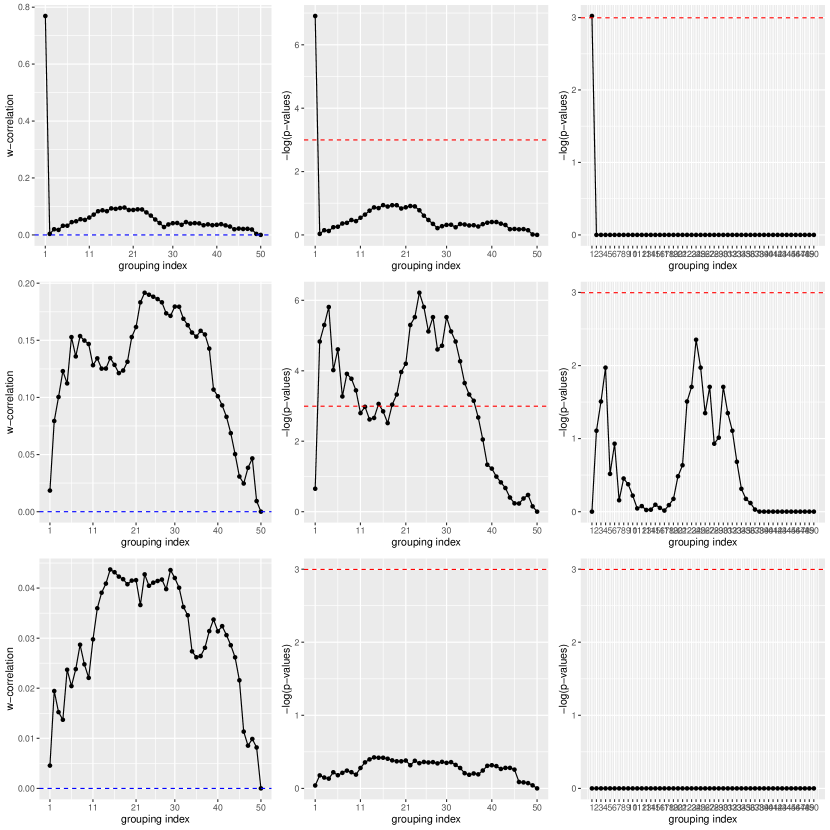
Figure 1: Simulations of three series in Example 1 with SNR = 5: ${w}$-correlation (left panels), raw and adjusted p-values (middle and right panels, respectively) in $-\log$ scale for different grouping indices. The blue dashed line denotes a ${w}$-correlation of zero, as assumed under the null hypothesis, while the red dashed line denotes the significance level $\alpha=0.05$.

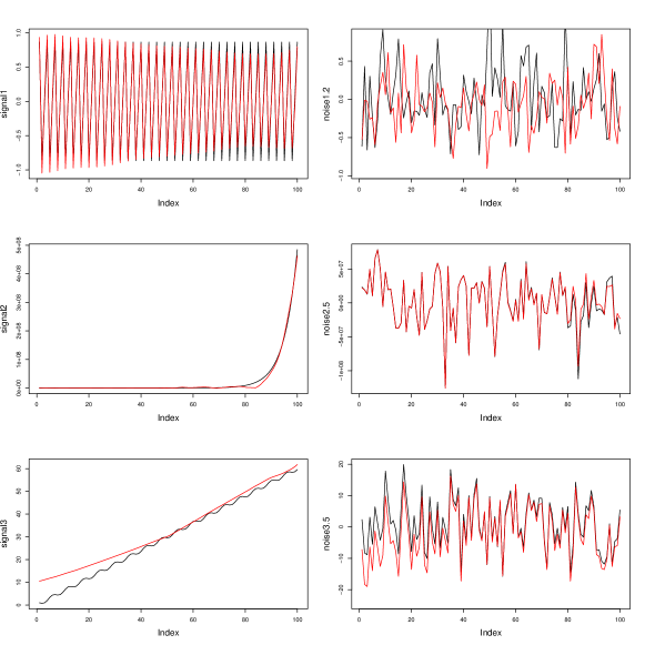
Figure 2: Simulations of three series in Example 1 with SNR = 5: visualizing the impact of the proposed grouping method for denoising. Black lines denote the simulated true main signal (left panels) and noise (right panels), while the red lines denote the corresponding reconstructions.

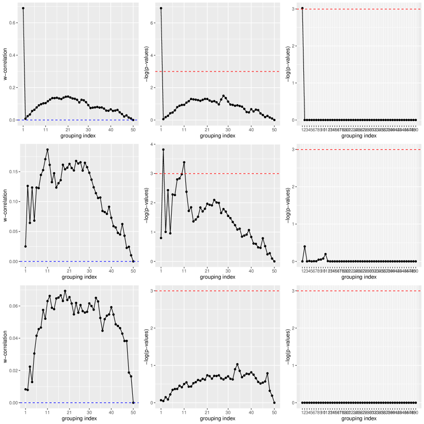
Figure 3: Simulations of three series in Example 1 with SNR = 2: ${w}$-correlation (left panels), raw and adjusted p-values (middle and right panels, respectively) in $-\log$ scale for different grouping indices. The blue dashed line denotes a ${w}$-correlation of zero, as assumed under the null hypothesis, while the red dashed line denotes the significance level $\alpha=0.05$.

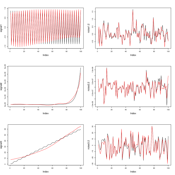
Figure 4: Simulations of three series in Example 1 with SNR = 2: visualizing the impact of the proposed grouping method for denoising. Black lines denote the simulated main signal (left panels) and noise (right panels), while the red lines denote the corresponding reconstructions.

FWER control is demonstrated in Table 1, which displays the empirical FWER, i.e., the proportion of repetitions where at least one true null hypothesis is falsely rejected or, in our case equivalently, the number of repetitions where the resulting grouping index is larger than the optimal one.

The empirical FWER never exceeds the significance level $\alpha=0.05$, which suggests that the FWER is controlled in all settings.

Time series	SNR=5		SNR=2
	FWER	Equal	FWER	Equal
$f_{1}$	0.00	1.00	0.00	1.00
$f_{2}$	0.00	1.00	0.00	1.00
$f_{3}$	0.00	1.00	0.00	1.00

Table 1: Performance of the proposed procedure based on Šidák correction: The column ”FWER” shows the proportion of times where the grouping index is higher than the real one; and the column ”Equal” is the proportion of times where optimal grouping index is exactly equal to the true optimal grouping index.

More importantly, Table 1 also displays the proportion of repetitions where the resulting grouping index is exactly equal to the optimal one. In all settings $f_{i}$, $i=\{1,2,3\}$, this proportion is equal to one for both SNRs, showing that the method was always able to capture the optimal grouping without under- or overestimating it, and so without wrongly mixing part of the main signal into the noise component or vice versa.
The proposed procedure based on Bonferroni-Holm correction yields similar results to those achieved using Šidák correction. Therefore, assuming a more general dependency structure seems seems to be possible without the cost of power (i.e., more frequent underestimation the optimal grouping index) for our procedure.

Next, we assess the denoising performance of SSA based on the obtained $g^{*}$ compared to selected $g\in\{1,2,\ldots,d-1\}\setminus\{g^{*}\}$. To do this, we assess the performance using criteria such as relative root mean squared error (RRMSE) and relative mean absolute error (RMAE), calculated using $g^{*}$ and the alternative $g$ values, which are given by

RRMSE $$= \frac{\left(\sum_{t=1}^{N}(f(t)-\hat{f}(t))^{2}\right)^{1/2}}{\left(\sum_{t=1}^{N}(f(t)-\tilde{f}(t))^{2}\right)^{1/2}},$$ (9)

RMAE $$= \frac{\sum_{t=1}^{N}\lvert f(t)-\hat{f}(t)\rvert}{\sum_{t=1}^{N}\lvert f(t)-\tilde{f}(t)\rvert},$$ (10)

where, $\hat{f}(t)$ represents the estimated value of $f(t)$ derived from SSA using $g^{*}$, while $\tilde{f}(t)$ denotes the estimated value of $f(t)$ obtained by employing alternative $g$ values. If $\text{RRMSE}<1$ or $\text{RMAE}<1$, then the estimated value of $f(t)$ derived from SSA using $g^{*}$ outperforms the estimated value of $f(t)$ obtained by applying alternative $g$ values by $(1-\text{RRMSE})\times 100\%$ or $(1-\text{RMAE})\times 100\%$, respectively.
Table 2 showcases the averaged RRMSE and RMAE values across various $g$ values, chosen from the vector $\{5,10,15,20,30\}$, excluding $g^{*}$ when necessary. The value of $g^{*}$ is set equal to the observed $g^{*}$ in the simulation study presented above. The average RRMSE and RMAE are computed based on $1000$ Monte Carlo repetitions. The results in Table 2 illustrate that the SSA method, when applying $g^{*}$, exhibits higher accuracy in signal extraction compared to the other considered $g$ values. This accuracy improvement is observed across all three considered time series for a window length of $L=50$.

In summary, the results of this simulation study underscore the significance of our proposed method in achieving optimal separability for different data scenarios and different SNRs. We demonstrated that using the Šidák or the Bonferroni-Holm procedure to correct for multiplicity in our procedure leads to similar results. Therefore, we recommend to apply the Bonferroni-Holm adjustment in practice, as it accounts for any arbitrary dependency structure of the p-values.

Time series	SNR=5		SNR=2
	RRMSE	RMAE	RRMSE	RMAE
$f_{1}$	0.32	0.33	0.32	0.33
$f_{2}$	0.24	0.17	0.25	0.18
$f_{3}$	0.62	0.59	0.41	0.40

Table 2: Comparison of average RRMSE and RMAE in the reconstructing time series using SSA method with $g^{*}$ against alternative $g$ Values.

5 Real-world Data Analysis

In this section we demonstrate the application of the proposed procedure to neuroimaging data. SSA is applied to data of various neurimaging techniques such as electroencephaogram (EEG) data, functional near infrared spectroscopy (fNIRS) data and functional magnetic resonance imaging (fMRI) data. Often, SSA is utilized for the identification of noise components in the observed signal (see e.g. Maddirala2016 for EEG, Spyrou2014 for fNRIS, Piaggi2014 for fMRI). In this section, we focus on the application of SSA to fMRI data. The observed signal in fMRI data is called the blood oxygen level dependent (BOLD) signal, which is used to draw conclusions about the neuronal activities of the brain. This can be done either for resting state fMRI (subject is not exposed to external stimulus) or event-related fMRI (subject is exposed to external stimuli, e.g., visual or auditory) [Poldrack2011]. For screening, i.e., collection of fMRI data, the brain is partitioned into a three dimensional grid and the time series of the BOLD signal is measured at each grid cell, the so-called voxels [Poldrack2011]. The BOLD signal contains, next to the hemodynamic response to neuronal activities, random and physiological noise. The latter includes for example signals from respiratory or cardiac processes, which have a broad range of frequencies [Piaggi2014]. Thus, bandpass filtering the observed BOLD signal, which removes high and low frequencies as defined by the practitioner, can be ineffective for noise reduction and might even remove some of the signal of interest [Piaggi2014, Poldrack2011]. Alternatively, SSA can be utilized to identify components of the BOLD time series which correspond to signal and noise, respectively.
We have applied the proposed procedure to resting state fMRI data, using the average BOLD time series of one region as demonstration, with the goal of differentiating signal from noise, i.e., investigating the trend in the observed BOLD signal. We have analyzed fMRI data collected by Wahlheim2021data and available at https://openneuro.org/datasets/ds003871/versions/1.0.2. The data include fMRI scans of 62 subjects who were required to move as little as possible and keep their eyes open during scanning. In total, $N=300$ scans were acquired for each subject, which defines the length of the BOLD signal time series for each voxel within a subjects brain. For more detailed information on data acquisition, see Wahlheim2022. From these 62 subjects, we have chosen the data of one subject (sub-1004 in Wahlheim2021data) to apply the proposed methodology. First, we have preprocessed the data, this includes slice time correction, performed using the R package ”fmri” [Rfmri], and motion correction, which has been performed using the software FSL [FSL]. Then, in accordance with Piaggi2014, we have used the observed BOLD response of voxels within the Middle Frontal Gyrus. To increase the SNR, we have averaged the BOLD signal of all voxels within this region for further analysis. We have then applied the methodology introduced in section 3 to the mean BOLD signal time series of this region, using for the SSA analysis a window length of $L=N/2=150$. The proposed procedure with $\alpha=0.05$ and utilization of the Bonferroni-Holm correction returns an optimal grouping of $g^{*}=1$. This is in line with the values of the ${w}$-correlation, which are at most $0.0004$. Based on the ${w}$-correlation matrix, illustrated in the right plot of Figure 5, one could use either the first two or three eigenvalues to reconstruct the time series. The lower left plot in Figure 5 displays the time series of the BOLD signal of the voxel under consideration in black; the reconstructed signal with grouping based on the proposed methodology corresponds to the red line and grouping based on the matrix of the $w$-correlation, that is, using a grouping index of two, is shown as a blue dotted line. These reconstructed time series indicate that using a grouping index based on the proposed procedure is better for distinguishing between the signal and noise than grouping indices defined based on the ${w}$-correlation matrix.

Figure 5: Illustration of SSA results: Analysis of the average BOLD signal time series of the Middle Frontal Gyrus with $N=300$ time points. The plot on the right displays the matrix illustration of the ${w}$-correlations. The lower plot on the left displays the preprocessed BOLD signal of the voxel under consideration as black line. The reconstructed signal based on the grouping according to the proposed procedure corresponds to the red line, while the blue dotted line correspond to the reconstructed signal based on the grouping derived from the $w$-correlation matrix.

6 Conclusion and Future Work

In this work we have derived a procedure to identify the best grouping for separation of a time series into signal and noise in the context of SSA. We assume separability if the $w$-correlation is close to zero. Thus, we find the best grouping by testing the null hypothesis of separability for all possible grouping indices and define the optimal grouping index $g^{*}$ as the minimal index for which the null hypotheses cannot be rejected for all $g\in\{g^{*},\ldots,d-1\}$. To account for the multiplicity of this approach, the Bonferroni-Holm procedure can be used to control the FWER. This procedure has the advantage of assuming an arbitrary dependency structure of the test statistics. We have thoroughly investigated the performance of the proposed procedure in a simulation study and applied it to the real world problem of distinguishing signal from noise in the observed time series of fMRI data.
The evaluation of the SSA method across various $g$ values highlights the significance of $g^{*}$ derived through the wild bootstrap method. The simulation studies demonstrate the superior performance of $g^{*}$ over other $g$ values, as evidenced by notable improvements in accuracy metrics such as RRMSE and RMAE.
This study opens avenues for future investigations. Further exploration could delve into refining the parameterization of the SSA method, investigating the impact of different parameter choices beyond $g$, and expanding the evaluation across diverse datasets. Moreover, extending this method’s application to practical scenarios and different types of time series data would be valuable. Additionally, exploring variations or enhancements of the SSA method could lead to improved accuracy and broader applicability in various domains.
In essence, the findings of this study underscore the potential of $g^{*}$ and lay the groundwork for future research directions aimed at enhancing the performance and applicability of the SSA method in time series analysis.