Intersystem Bell-like States in Classical Polarization Optics

Abstract

A method is proposed to produce a classical optical state that is ‘intersystem nonseparable’ and a close analog of the $\phi^{+}$ Bell state. A derivation of the CHSH-Bell inequality is sketched within the framework of classical polarization optics using noncontextuality for factorizable states as an axiom rather than any hidden variable theory, and it is shown that the classical state violates this inequality.

1 Introduction

There is some controversy in the literature as to whether the nonseparability that has been observed in classical light should be called ‘entanglement’ because entanglement is a term coined by Schrödinger specifically to express a purely quantum nonseparability that persists in spite of arbitrary spatial separation of the sub-systems [1] (2019). It is true that most instances of nonseparability observed with classical light so far are of a local nature, involving different modes (DoFs) of the same optical beam [2, 3]. They have been termed ‘intra-system noneparability’ or ‘classical entanglement’ as opposed to ‘quantum entanglement’ which is believed (by the majority of physicists) to imply nonlocality [4]. It is also generally believed that only intrasystem nonseparability has a classical analogy, though there is no proof.

It is therefore important to investigate whether ‘intersystem nonseparability’ also has any classical analog, and if so, what it implies. In this paper I will first propose a method of producing an intersystem nonseparable state in classical polarization optics, and then explore to what extent it is quantum-like.

To describe polarized light it is most convenient to use normalized Jones vectors

$$|J\rangle=\frac{1}{\sqrt{\langle J|J\rangle}}\left(\begin{array}[]{c}E_{x}\\ E_{y}\end{array}\right)$$ (1)

with $E_{x}=A_{0}\hat{e}_{x}{\rm exp(i\phi_{x})}$ and $E_{y}=A_{0}\hat{e}_{y}{\rm exp(i\phi_{y})}$ the complex transverse electric fields, $\hat{e}_{x}$ and $\hat{e}_{y}$ the unit polarization vectors, and $\langle J|J\rangle=|E_{x}|^{2}+|E_{y}|^{2}=A_{0}^{2}$, the intensity $I_{0}$. This is a column vector in a 2-dimensional Hilbert space of polarization states. The Jones vector for horizontally ($x$ axis) polarized light is

$$|h\rangle\equiv|1\rangle=\left(\begin{array}[]{c}1\\ 0\end{array}\right),$$ (2)

and that of vertically polarized ($y$ axis) light is

$$|v\rangle\equiv|0\rangle=\left(\begin{array}[]{c}0\\ 1\end{array}\right).$$ (3)

Jones vectors for other linear polarization states can be written as linear combinations of these basis vectors.

2 How to Produce a Classical Bell-like State

Let us now briefly recollect the standard procedure for producing the first Bell state in quantum mechanics. One uses a two-qubit circuit consisting of a Hadamard gate H and a CNOT gate. The Hadamard gate applied to a general qubit gives $H|q\rangle=\frac{1}{\sqrt{2}}[|0\rangle+|1\rangle]$. This state combined with a $|0\rangle$ state produces the state $\frac{1}{\sqrt{2}}[|0\rangle\otimes|0\rangle+|1\rangle\otimes|0\rangle]$, and the CNOT gate produces the Bell state $\frac{1}{\sqrt{2}}[|0\rangle\otimes|0\rangle+|1\rangle\otimes|1\rangle]$.

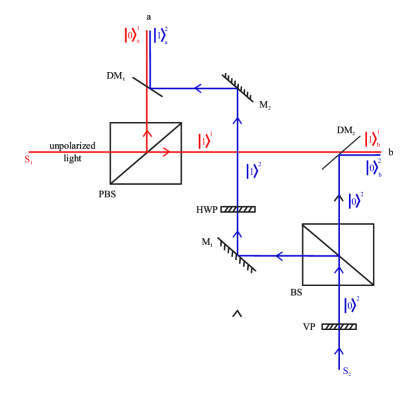
Figure 1: Schematic diagram to produce a classical analog of the first Bell state.

Let us now see how this circuit can be realized in classical optics. Consider two quasi-monochromatic sources $S_{1}$ and $S_{2}$ of classical light of equal intensities but different mean angular frequencies $\omega_{1}$ (denoted by red in the figure) and $\omega_{2}$ (denoted by blue in the figure). Let the beam emitted by $S_{1}$ be unpolarized and that emitted by $S_{2}$, also unpolarized, be converted to a vertically polarized beam $|0\rangle_{2}$ by passing through a vertical polarizer VP. These correspond to the qubit $|q\rangle$ and $|0\rangle$. Let the unpolarized beam (red) be incident on a polarizing beam splitter PBS as shown in the figure. It acts like a Hadamard gate, producing the polarization state $\frac{1}{\sqrt{2}}[i|0\rangle_{1}^{a}+|1\rangle_{1}^{b}]$, the reflected light being vertically polarized ($|0\rangle$) and the transmitted light horizontally polarized ($|1\rangle$). Let the second beam (vertically polarized $|0\rangle_{2}$ and blue) be incident on an ordinary beam splitter BS. The part of the beam transmitted by BS is combined with the horizontally polarized beam transmitted by PBS by means of a dichroic mirror $DM_{2}$. The part of the beam reflected by BS is first reflected by a lossless mirror $M_{1}$, passes throgh a half-wave plate HWP, gets converted into a horizontally polarized beam $|1\rangle_{2}$ which is then reflected by a lossless mirror $M_{2}$ and combined with the vertically polarized red beam reflected by PBS by means of a dichroic mirror $DM_{1}$.The beam splitter BS and the half-wave plate HWP thus act like a CNOT gate, and the final polarization state of the output beams $a$ and $b$ is

$$|\phi^{+}\rangle=\frac{i}{\sqrt{2}}\left[|0\rangle_{1}^{a}\otimes|0\rangle_{2}^{b}+|1\rangle_{1}^{b}\otimes|1\rangle_{2}^{a}\right].$$ (4)

This is a nonseparable/nonfactorizable state. It is precisely what we were looking for, namely ‘intersystem nonseparability’ of classical light, a nonseparability that persists in spite of arbitrary spatial separation of the sub-systems. The three other Bell-like nonseparable states can be produced by using variations of this method.

Let us see to what extent such states are quantum-like. Shimony [5] has listed the following three criteria that any system S produced for testing its quantum nature must satisfy:

(I) In any state of a physical system S there are some eventualities which have indefinite truth values.

(II) If an operation is performed which forces an eventuality with indefinite truth value to achieve definiteness … the outcome is a matter of chance.

(III) There are ‘entangled systems’ (in Schrödinger’s phrase) which have the property that they constitute a composite system in a pure state, while neither of them separately is in a pure state.

The state (4) clearly satifies criterion (III). As regards the other two criteria, it would be useful to consider thermal light. In particular, let $S_{1}$ and $S_{2}$ be two thermal sources which are wide-sense stationary. In a beam of thermal light the value of the ‘optical field’ is unpredictable. The observable optical field of such a light beam is the space-time dependent electric field vector

$$\vec{E}(r,t)=\hat{h}E_{h}(r,t)+\hat{v}E_{v}(r,t)$$ (5)

where $\hat{h}$ and $\hat{v}$ are orthogonal and arbitrarily oriented ‘horizontal’ and ‘vertical’ polarization directions, and the amplitudes $E_{h}(r,t)=\sum_{n}h_{n}(t)\phi_{n}(r)$ and $E_{v}(r,t)=\sum_{l}v_{l}(t)\phi_{l}(r)$ are statistically completely uncorrelated, being elements of a stochastic function space. Scalar products of the vectors in this space correspond physically to observable correlation functions such as $\langle E_{v}E_{h}\rangle$, the angular bracket denoting expectation value. For unpolarized light $\langle E_{v}E_{v}\rangle=\langle E_{h}E_{h}\rangle$ and $\langle E_{v}E_{h}\rangle=0$. The $\phi_{n}(r)$ are orthonormal spatial mode functions with $\int dr\phi^{*}_{n}(r)\phi_{l}(r)=\delta_{n,l}$, and $h_{n}(t)$ and $v_{l}(t)$ represent stochastic random coefficients whose origin one can assign to distant and unknowable dipole radiators.

Since the value of $\vec{E}$ in thermal light is unpredictable at any time, and a definite truth value is obtained only when the field is appropriately detected, Shimony’s criteria (I) and (II) are also satisfied. Nevertheless, this picture of the optical field does not imply that it is quantized, only a non-deterministic viewpoint is employed to extract predictions from the randomly unknown ensemble of field potentialities.

Since the red beam with frequency $\omega_{1}$ is unpolarized,

$$\langle E_{1v}(r,t),E_{1h}(r,t)\rangle = 0,$$ (6)

$$\langle E^{*}_{1v}(r,t),E_{1v}(r,t)\rangle = \langle E^{*}_{1h}(r,t),E_{1h}(r,t)\rangle$$ (7)

for all $(r,t)$ [6]. Since this unpolarized red beam splits into vertical and horizontal components at some point within the beam splitter PBS (as shown in Fig. 1), the first equation (6) implies that the red beams in paths $a$ and $b$ are completely uncorrelated. In other words, the red beam will exhibit anticoincidence on the beam splitter, a quantum-like feature. The second result (7) implies that the measured intensities of the vertical and horizontal components are always equal everywhere in the beams.

Now, the classical electrical fields in the two paths $a$ and $b$ (Fig. 1) are (see Appendix)

$$\vec{E}^{a}(r_{a},t) = \hat{v}E^{a}_{1v}(r_{a},t)+\hat{h}E^{a}_{2h}(r_{a},t),$$ (8)

$$\vec{E}^{b}(r_{b},t) = \hat{h}E^{b}_{1h}(r_{b},t)+\hat{v}E^{b}_{2v}(r_{b},t).$$ (9)

They fluctuate stationarily in the wide-sense. Since the sources $S_{1}$ and $S_{2}$ are independent, the following first-order cross correlations vanish, namely

$$\langle E^{a*}_{1v}(r_{a},t),E^{a}_{2h}(r_{a},t+\tau)\rangle = \langle E^{b*}_{2v}(r_{b},t),E^{b}_{1h}(r_{b},t+\tau)\rangle=0,$$ (10)

$$\langle E^{a*}_{1v}(r_{a},t),E^{b}_{2v}(r_{b},t)\rangle = \langle E^{a*}_{2h}(r_{a},t),E^{b}_{1h}(r_{b},t)\rangle=0.$$ (11)

Eqn (10) implies that red and blue lights (which, by experimental design, always have orthogonal polarizations in each path) are completely uncorrelated in each path. These results guarantee randomness of outcomes (red/blue) in each path/end, another quantum-like feature. Eqn (11) shows that the vertically polarized red beam in path $a$ and the vertically polarized blue beam in path $b$ are uncorrelated, and so also are the horizontally polarized red beam in path $b$ and the horizontally polarized blue beam in path $a$, in spite of the light being in the nonseparable polarization state (4). This guarantees that ‘superluminal signalling’ does not occur at the statistical level, which is also a quantum-like feature.

These results demonstrate to what extent intersystem nonseparability in classical optics is similar to that in quantum optics.

3 CHSH-Bell Inequality

The question that arises therefore is: does intersystem nonseparability of classical light imply any Bell violation which is usually taken as a measure of nonlocality? To see that, consider a classical separable state like

$$\frac{1}{\sqrt{2}}(\left[|1\rangle\otimes|0\rangle+|0\rangle\otimes|0\rangle\right]=\left[|1\rangle+|0\rangle\right]\otimes|0\rangle$$ (12)

and joint polarization measurements on the two sides $a$ and $b$ at angles $(\theta_{a},\theta_{a^{\prime}})$ and $(\theta_{b},\theta_{b^{\prime}})$. Instead of local realism, assume only noncontextuality which is the requirement that the result of a measurement is predetermined and not affected by how the value is measured, i.e. not affected by previous or simultaneous measurement of any other compatible or co-measureable observable. Treating the normalized classical Jones vectors mathematically as qubits, one can then quite easily derive the CHSH inequality [9, 10]

$$-2\leq E(\theta_{a},\theta_{b})-E(\theta_{a},\theta_{b^{\prime}})+E(\theta_{a^{\prime}},\theta_{b})+E(\theta_{a^{\prime}},\theta_{b^{\prime}})\leq+2$$ (13)

where $E(\theta_{a},\theta_{b})$ are expectation values. [The outcomes need not be $\pm 1$ as is usually assumed. It is sufficient that they lie between $\pm 1$ which is guaranteed by Malus’ Law in classical polarization optics with normalized Jones vectors [11].] If the nonseparable state (4) is used, one gets

$$E(\theta_{a},\theta_{b})=\cos(\theta_{a}-\theta_{b}),$$ (14)

and for a specific set of values $\theta_{a}=\pi/2,\theta_{a^{\prime}}=0,\theta_{b}=\pi/4,\theta_{b^{\prime}}=-\pi/4$ one gets $S=2\sqrt{2}$ which violates the CHSH inequality.

The original derivations of the Bell and CHSH inequalities involved the use of local hidden variables (local realism). Hence, in such a framework a CHSH violation would rule out local hidden variable theories. If the hidden variables are noncontextual (Einstein realism), nonlocality would follow. To avoid nonlocality, one must assume a reality that is contextual (as Bohr did in terms of his complementarity idea).

As we have just seen, Bell-CHSH inequalities can also be derived within the framework of classical polarization optics using noncontextuality. Hence, a CHSH violation with spatially separated subsystems in classical polarization optics would imply a violation of noncontextuality rather than of locality [12, 13], signalling a radical change in the very notion of classical realism, namely a reality that is contextual.

4 Concluding Remarks

I have proposed a method to produce a classical optical state that is (a) ‘intersystem nonseparable’, (b) statistically close to a Bell state and (c) violates the Bell-CHSH inequality without violating locality. Hence, intersystem nonseparability per se does not imply nonlocality.

Having said that, it is important to point out a crucial difference between classical and quantum nonseparable states, namely that the statistics can never be sub-Poissonian with classical light.

5 Appendix

To see that the electric fields (8) and (9) indeed represent the polarization state (4), consider the corresponding states

$$|{\cal{E}}^{a}\rangle = e^{a}_{1v}|0\rangle^{a}_{1}+e^{a}_{2h}|1\rangle^{a}_{2},$$ (15)

$$|{\cal{E}}^{b}\rangle = e^{b}_{1h}|1\rangle^{b}_{1}+e^{b}_{2v}|0\rangle^{b}_{2},$$ (16)

where $e^{a}_{1v}$ etc are the normalized electric field components. Then, the normalized tensor product of the two independent light beams is

$$\frac{1}{\sqrt{2}}\left[e^{a}_{1v}e^{b}_{2v}|0\rangle^{a}_{1}\otimes|0\rangle^{b}_{2}+e^{b}_{1h}e^{a}_{2h}|1\rangle^{b}_{1}\otimes|1\rangle^{a}_{2}\right].$$ (17)

The normalized electric field coefficients are usually omitted in writing Bell-like states.

To produce the nonseparable polarization state

$$|\psi^{+}\rangle=\frac{i}{\sqrt{2}}\left[|0\rangle_{1}^{a}\otimes|1\rangle_{2}^{b}+|1\rangle_{1}^{b}\otimes|0\rangle_{2}^{a}\right],$$ (18)

the experimental set up needs to be a variant of the one proposed here, namely one using the scheme $H|q\rangle\otimes|1\rangle=\frac{1}{\sqrt{2}}[|0\rangle+|1\rangle]\otimes|1\rangle=\frac{1}{\sqrt{2}}[|0\rangle\otimes|1\rangle+|1\rangle\otimes|1\rangle]$ followed by a CNOT gate. This means replacing the vertical polarizer VP in the path of the $S_{2}$ beam (Fig. 1) by a horizontal polarizer VH. Then the electrical fields in the two paths are

$$\vec{E}^{a}(r_{a},t) = \hat{v}E^{a}_{1v}(r_{a},t)+\hat{v}E^{a}_{2v}(r_{a},t),$$ (19)

$$\vec{E}^{b}(r_{b},t) = \hat{h}E^{b}_{1h}(r_{b},t)+\hat{h}E^{b}_{2h}(r_{b},t),$$ (20)

corresponding to the polarization state (18).

6 Acknowledgement

The author is grateful to C. S. Unnikrishnan, G. Raghavan and members of the School of Quantum Technologies, DIAT, Pune for helpful discussions on the difference between quantum and classical entanglement.

References

- [1] D. Paneru, E. Cohen, R. Fickler, R. W. Boyd and E. Karimi1, arXiv:1911.02201 [quant-ph] (2019) and references therein
- [2] X-F Qian, B. Little, J. C. Howell and J. H. Eberly, ‘Violation of Bell’s Inequalities with Classical Shimony-Wolf States: Theory and Experiment’, arXiv:1406.3338 [quant-ph] (2014).
-
[3]
X-F Qian, B. Little, J. C. Howell, AND J. H. Eberly,
bf 2 (7), 611-615 (2015). - [4] A. Aiello, F. Töppel1, C. Marquardt, E. Giacobino and G. Leuchs, New J. of Phys. 17, 043024 (2015).
- [5] A. Shimony, Brit. J. Phil. Sci. 35, 25-45 (1984).
- [6] X-F Qian, B. Little, J. C. Howell, and J. H. Eberly, Optica 2 (7), 611-615 (2015).
- [7] C. Brosseau, Fundamentals of Polarized Light: A Statistical Optics Approach, Wiley, New York (1998).
- [8] E. Wolf, Introduction to the Theory of Coherence and Polarization of Light, Cambridge Univ. Press (2007).
- [9] J. F. Clauser, M. A. Horne, A. Shimony and R. A. Holt, Phys. Rev. Lett. 23 (15), 880–4, (1969).
- [10] J.S. Bell, Physics 1 (3), 195-200 (1964), reproduced as Ch. 2 of J. S. Bell, Speakable and Unspeakable in Quantum Mechanics, Cambridge University Press (2004).
- [11] P. Ghose and A. Mukherjee, Adv. Sc., Eng. and Med. 6, 246-251 (2014).
- [12] A. Khrennikov, Quantum versus classical entanglement: eliminating the issue of quantum nonlocality. arXiv:1909.00267v1 [quant-ph].
- [13] A. Khrennikov, Two faced Janus of quantum nonlocality. arXiv: 2001.02977v1 [quant-ph].