Fermion states localized on a self-gravitating Skyrmion

Abstract

We investigate self-gravitating solutions of the Einstein-Skyrme theory coupled to spin-isospin Dirac fermions and consider the dependence of the spectral flow on the effective gravitational coupling constant and on the Yukawa coupling. It is shown that the effects of the backreaction of the fermionic mode may strongly deform the configuration. In particular, the energy conditions may be violated, and regular anti-gravitating asymptotically flat solutions with negative ADM mass may emerge.

I Introduction

There are various classical field theories that admit topologically stable soliton solutions. These are particle-like regular localized field configurations with finite energy. Famous examples of such topological solitons in (3+1)-dimensions are monopoles in the Yang-Mills-Higgs model [1, 2], Skyrmions [3, 4] and Hopfions [5, 6] (for reviews, see, for example, Refs. [7, 8]). In particular, the groundbreaking work by Skyrme [3, 4] gave rise to an increasing interest in the study of various aspects of such solutions in a wide variety of physical systems, both in flat and curved spacetime.

Flat space topological solitons can be minimally coupled to gravity. The emerging systems of Einstein-matter field equations may then support the existence of gravitating spatially localized globally regular solutions and of black holes. Endowing the gravitating soliton solutions with an event horizon, the so-called hairy black holes arise, which possess nontrivial matter fields outside their event horizon, i.e., they carry hair (see, e.g., Refs. [9, 10]). Well-known examples include self-gravitating monopoles [11, 12, 13] and Skyrmions [14, 15, 16, 17, 18, 19].

A peculiar feature of topological solitons is the link between the topological charge of the configuration and the number of quasi-zero fermionic modes localized on the soliton. The fundamental Atiyah-Patodi-Singer index theorem [20] yields a remarkable relation between these quantities. The spectrum of the fermions in the background of a soliton of topological degree one shows a spectral flow of the eigenvalues with one normalizable bound mode crossing zero.

Fermionic modes localized on solitons were first discussed in the pioneering work [21]. Later, it was shown that such bound states exist on kinks [22, 23, 24], domain walls [25], monopoles [26, 27], sphalerons [28, 29], and Skyrmions [30, 31, 32]. The presence of localized fermion modes gives rise to interesting phenomena like monopole catalysis of proton decay [26, 27], emergence of superconducting cosmic strings [33], and appearance of fractional quantum numbers of solitons [22, 34].

A major simplification of most of these studies is that, until recently, the backreaction of the soliton was not taken into account. This assumption is justified in the weak coupling limit. However, as the Yukawa coupling increases, the effects of the backreaction can be significant, see Refs. [35, 36, 37, 38, 39, 40, 41, 42, 43, 44, 45].

As compared to boson fields, fermions have attracted less attention in General Relativity. Although solutions of the Dirac equation in curved spacetime were constructed many decades ago [46], the consideration of self-gravitating fermions still remains somewhat obscure, because the Dirac field has to be treated in terms of a normalizable quantum wave function and the corresponding particle number is restricted by Pauli’s exclusion principle. However, one can make use of the approximation that (i) only single-particle fermion states are considered, and (ii) second quantization of the fields is ignored, and gravity is treated purely classically. Under these assumptions, for instance, the fermion level crossing in the background of the Einstein-Yang-Mills sphaleron was considered in Ref. [47]. It then turns out that self-gravitating spinor fields may give rise to some interesting phenomena in the cosmology of the accelerating Universe [48, 49]. It has also been shown that the Einstein-Dirac equations support regular localized solitonic solutions [50], the so-called Dirac stars [51, 52, 53, 54, 55]. Moreover, the backreaction of self-gravitating fermions may significantly affect the metric and, in particular, allow for (traversable) wormholes [56, 57, 58].

A system of coupled gravitating bosonic and fermionic fields was first studied in Ref. [59]. The dynamical evolution of the spherically symmetric fermionic zero mode localized on the self-gravitating $SU(2)$ monopole was studied recently in Ref. [60]. The main objective of the present paper is to examine a similar system of a spherically symmetric spin-isospin fermionic mode localized on the self-gravitating Skyrmion, where for consistency the backreaction of the fermions on the Skyrme field and on the metric is taken into account. It is known that, although in flat space both topological solitons, the monopole and the Skyrmion, support a localized fermionic (quasi) zero mode, the pattern of evolution of these solitons is different, as gravity is taken into account. While the monopole solutions of the Einstein-Yang-Mills-Higgs model are linked to the Reissner-Nordström black hole [11, 12, 13], the gravitating Skyrmions possess the Bartnik-McKinnon (BM) limit [15, 18, 17, 19]). Therefore, it is of interest to investigate the fate of the backreacting Skyrmion-fermion system as the coupling to gravity is varied.

II The Model

We consider the (3+1)-dimensional Einstein-Skyrme system, coupled to a spin-isospin field $\psi_{\alpha i}$

$$S=\int d^{4}x\sqrt{-\cal g}\left(-\frac{R}{16\pi G}+{\cal L}_{m}\right)\ ,$$ (1)

where the gravitational part is the usual Einstein-Hilbert action, $\cal g$ is the determinant of the metric, $R$ is the curvature scalar, and $G$ is Newton’s constant. The Lagrangian of the matter fields ${\cal L}_{m}$ is given in terms of the Skyrme field $U\in SU(2)$ [3, 4] minimally coupled to the Dirac isospinor fermions $\psi_{\alpha i}$, ${\cal L}_{m}={\cal L}_{\text{Sk}}+{\cal L}_{\text{sp}}+{\cal L}_{\text{int}}$. We consider the usual Lagrangian of the Skyrme model without a potential term

$${\cal L}_{\text{Sk}}=-\frac{f_{\pi}^{2}}{4}\,\,\mbox{Tr}\left(\partial_{\mu}U\,\partial^{\mu}U^{\dagger}\right)+\frac{1}{32\,a_{0}^{2}}\,\mbox{Tr}\left(\left[\partial_{\mu}U\,U^{\dagger},\,\partial_{\nu}U\,U^{\dagger}\right]^{2}\right)\,.$$ (2)

Here $f_{\pi}$ and $a_{0}$ are the parameters of the model with dimensions $[f_{\pi}]=L^{-1}$ and $[a_{0}]=L^{0}$, respectively.

The matrix-valued field $U$ can be decomposed into the scalar component $\phi_{0}$ and the pion isotriplet $\phi_{k}$ via

$$U=\phi_{0}\,\mathbb{I}+i\,\sum_{n=1}^{3}\phi_{n}\,\tau_{n}\ ,$$ (3)

where $\tau_{n}$ are the Pauli matrices, and the field components $\phi^{a}=(\phi_{0},\phi_{k})$ are subject to the sigma-model constraint, $\phi^{a}\cdot\phi^{a}=1$.

The Skyrme field is required to attain its vacuum value, the identity, at spatial infinity, $U\xrightarrow[\vec{r}\to\infty]{}{\mathbb{I}}$. It is a map $U:S^{3}\mapsto S^{3}$ characterized by an integer-valued winding number [3, 4].

The Dirac Lagrangian is

$${\cal L}_{\text{sp}}=\frac{\imath}{2}\left[(\hat{\not{D}}\bar{\psi})\psi-\bar{\psi}\hat{\not{D}}\psi\right]-m\bar{\psi}\psi\,,$$ (4)

where $m$ is a bare mass of the fermions, $\gamma^{\mu}$ are the Dirac matrices in the standard representation in a curved spacetime, $\hat{\not{D}}=\gamma^{\mu}\hat{D}_{\mu}$, and the isospinor covariant derivative on a curved spacetime is defined as (see, e.g., Ref. [61])

$$\hat{D}_{\mu}\psi=(\partial_{\mu}-\Gamma_{\mu})\psi.$$

Here $\Gamma_{\mu}$ are the spin connection matrices [62, 61].

Finally, the Skyrmion-fermion chiral interaction Lagrangian is

$${\cal L}_{\text{int}}=h\bar{\psi}\,U^{\gamma_{5}}\,\psi,\qquad U^{\gamma_{5}}\equiv\frac{\mathbb{I}+\tilde{\gamma}_{5}}{2}U+\frac{\mathbb{I}-\tilde{\gamma}_{5}}{2}U^{\dagger}\,,$$ (5)

where $h$ is the Yukawa coupling constant and $\tilde{\gamma}^{5}$ is the corresponding Dirac matrix in curved spacetime. Note that this matrix is the same both in flat and curved spacetime,

$$\begin{split}\tilde{\gamma}^{5}&=-\frac{\imath}{4!}E_{\alpha\beta\rho\sigma}\gamma^{\alpha}\gamma^{\beta}\gamma^{\rho}\gamma^{\sigma}=-\frac{\imath}{4!}\sqrt{-\cal g}\epsilon_{\alpha\beta\rho\sigma}e_{a}^{\alpha}e_{b}^{\beta}e_{c}^{\rho}e_{d}^{\sigma}\gamma^{a}\gamma^{b}\gamma^{c}\gamma^{d}\\ &=\frac{\sqrt{-\cal g}}{4!}\left(\epsilon_{\alpha\beta\rho\sigma}\epsilon^{abcd}e_{a}^{\alpha}e_{b}^{\beta}e_{c}^{\rho}e_{d}^{\sigma}\right)\gamma^{5}=\gamma^{5}\,.\end{split}$$ (6)

Here $E_{\alpha\beta\rho\sigma}=\sqrt{-\cal g}\epsilon_{\alpha\beta\rho\sigma}$ is the Levi-Civita tensor in curved spacetime and $\gamma^{5}=-\imath\gamma^{0}\gamma^{1}\gamma^{2}\gamma^{3}$ is the Dirac matrix in Minkowski spacetime.

It is convenient to introduce the dimensionless radial coordinate $\tilde{r}=a_{0}f_{\pi}r$, and the effective gravitational coupling $\alpha^{2}=4\pi Gf_{\pi}^{2}$, and to rescale the Dirac field, the Yukawa coupling constant and the bare fermion mass as $\psi\to\psi/\sqrt{a_{0}f_{\pi}^{3}}$, $h\to h/(a_{0}f_{\pi})$, and $m\to m/(a_{0}f_{\pi})$, respectively. We also introduce the dimensionless ADM mass $\tilde{M}=\alpha^{2}M/(4\pi f_{\pi}/a_{0})$ (for its explicit definition, see Eq. (26) below). Hereafter we drop the tilde in the dimensionless variables for the sake of brevity.

In terms of these units the Skyrme Lagrangian (2) can be written in component notation as

$${\cal L}_{\text{Sk}}=\partial_{\mu}\phi^{a}\partial^{\mu}\phi^{a}-\frac{1}{2}(\partial_{\mu}\phi^{a}\partial^{\mu}\phi^{a})^{2}+\frac{1}{2}(\partial_{\mu}\phi^{a}\partial_{\nu}\phi^{a})(\partial^{\mu}\phi^{b}\partial^{\nu}\phi^{b})\,.$$ (7)

The rescaled parity-invariant interaction Lagrangian (5) takes the form [63, 30, 31, 32, 64, 65]

$${\cal L}_{\text{int}}=h\bar{\psi}[\phi_{0}+i\gamma_{5}(\phi^{a}\cdot\sigma^{a})]\psi\,.$$

The corresponding components of the stress-energy tensor are

$$T^{\mu\nu}=T^{\mu\nu}_{\text{Sk}}+T^{\mu\nu}_{\text{sp}},$$ (8)

where the stress-energy tensor of the gravitating Skyrmion is

$$T^{\mu\nu}_{\text{Sk}}=2\,\left[\partial^{\mu}\phi_{a}\,\partial^{\nu}\phi^{a}-\left(\partial^{[\mu}\phi^{a}\,\partial^{\alpha]}\phi^{b}\right)\,\left(\partial^{[\nu}\phi_{a}\partial_{\alpha]}\phi_{b}\right)\right]-g^{\mu\nu}\,\left[\left(\partial_{\alpha}\phi_{a}\right)^{2}-\frac{1}{2}\left(\partial_{[\alpha}\phi_{a}\,\partial_{\beta]}\phi_{b}\right)^{2}\right]\,,$$ (9)

and the stress-energy tensor of the gravitating isospinor is

$$T^{\mu\nu}_{\text{sp}}=\frac{\imath}{4}\left[\bar{\psi}\gamma^{\mu}(\hat{D}^{\nu}\psi)+\bar{\psi}\gamma^{\nu}(\hat{D}^{\mu}\psi)-(\hat{D}^{\mu}\bar{\psi})\gamma^{\nu}\psi-(\hat{D}^{\nu}\bar{\psi})\gamma^{\mu}\psi\right]-g^{\mu\nu}{\cal L}_{\text{sp}}\,.$$ (10)

II.1 Spherically symmetric Ansatz and field equations

To construct static spherically symmetric solutions of the model (1) we employ Schwarzschild-like coordinates and adopt the spherically symmetric metric, following closely the usual consideration of self-gravitating Skyrmions (see, e.g., Refs. [15, 18, 17, 19]),

$$ds^{2}=\sigma^{2}(r)N(r)dt^{2}-\frac{dr^{2}}{N(r)}-r^{2}\left(d\theta^{2}+\sin^{2}\theta d\varphi^{2}\right).$$ (11)

The above metric implies the following form of the orthonormal tetrad:

$$e^{a}_{\phantom{a}\mu}=\text{diag}\left\{\sigma\sqrt{N},\frac{1}{\sqrt{N}},r,r\sin\theta\right\},$$

such that $ds^{2}=\eta_{ab}(e^{a}_{\mu}dx^{\mu})(e^{b}_{\nu}dx^{\nu})$, where $\eta_{ab}=(+1,-1,-1,-1)$ is the Minkowski metric. The Dirac matrices in the curved spacetime are then given by $\gamma^{\mu}=e^{\mu}_{\phantom{a}a}\hat{\gamma}^{a}$ with $\hat{\gamma}^{a}$ being the usual flat spacetime Dirac matrices.

For the static spherically symmetric Skyrmion of topological degree one, we make use of the usual hedgehog parametrization

$$U=\cos\left(F(r)\right)\mathbb{I}+\imath\sin\left(F(r)\right)\left(\sigma^{a}n^{a}\right)\,,$$ (12)

where $n^{a}=\{\sin(\theta)\cos(\varphi),\sin(\theta)\sin(\varphi),\cos(\theta)\}$. This Ansatz is in agreement with Eq. (3).

The spherically symmetric Ansatz with a harmonic time dependence for the isospinor fermion field localized on the Skyrmion can be written in terms of two $2\times 2$ matrices $\chi$ and $\eta$ [22, 66] as

$$\psi=e^{-\imath\omega t}\begin{pmatrix}\chi\\ \eta\end{pmatrix}\quad\text{with}\quad\chi=\frac{u(r)}{\sqrt{2}}\begin{pmatrix}0&-1\\ 1&0\end{pmatrix},\quad\eta=\imath\,\frac{v(r)}{\sqrt{2}}\begin{pmatrix}\sin\theta e^{-\imath\varphi}&-\cos\theta\\ -\cos\theta&-\sin\theta e^{\imath\varphi}\end{pmatrix}.$$ (13)

Here $u(r)$ and $v(r)$ are two real functions of the radial coordinate only and $\omega$ is the eigenvalue of the Dirac operator.

Substitution of the Ansatz (11)-(13) into the general action (1) yields the reduced Einstein-Hilbert Lagrangian

$${\cal L}_{\text{GR}}=-\frac{1}{2\alpha^{2}}\left(\frac{N^{\prime}}{r}+\frac{N-1}{r^{2}}\right),$$ (14)

while the Skyrme Lagrangian (7) becomes

$${\cal L}_{\text{Sk}}=-\frac{1}{2}\left[N(F^{\prime})^{2}+\frac{2\sin^{2}F}{r^{2}}\right]-\frac{\sin^{2}F}{r^{2}}\left[N(F^{\prime})^{2}+\frac{\sin^{2}F}{2r^{2}}\right]\,,$$ (15)

where a prime denotes a radial derivative. The fermion Lagrangian (4) is

$${\cal L}_{\text{sp}}=\sqrt{N}\left(vu^{\prime}-uv^{\prime}\right)-\frac{2uv}{r}+\frac{\omega\left(u^{2}+v^{2}\right)}{\sigma\sqrt{N}}+m\left(-u^{2}+v^{2}\right)\,,$$ (16)

and the interaction Lagrangian can be written as

$${\cal L}_{\text{int}}=h\left[\cos F(u^{2}-v^{2})-2uv\sin F\right]\,.$$ (17)

In the expressions (14)-(17), all the Lagrangians are rescaled as ${\cal L}\to{\cal L}/(a_{0}^{2}f_{\pi}^{4})$.

Next, multiplying the Lagrangians (14)-(17) by $\sqrt{-\cal g}$ and varying the total Lagrangian with respect to the functions $F,u,v,N,\sigma$, we get the following set of five coupled ordinary differential equations:

$$v^{\prime}+\left[\frac{N^{\prime}}{4N}+\frac{\sigma^{\prime}}{2\sigma}+\frac{1}{r}\left(1+\frac{1}{\sqrt{N}}\right)\right]v+\frac{h}{\sqrt{N}}\left(v\sin F-u\cos F\right)-\omega\frac{u}{N\sigma}+m\frac{u}{\sqrt{N}}= 0,$$ (18)

$$u^{\prime}+\left[\frac{N^{\prime}}{4N}+\frac{\sigma^{\prime}}{2\sigma}+\frac{1}{r}\left(1-\frac{1}{\sqrt{N}}\right)\right]u-\frac{h}{\sqrt{N}}\left(u\sin F+v\cos F\right)+\omega\frac{v}{N\sigma}+m\frac{v}{\sqrt{N}}= 0,$$ (19)

$$\begin{split}&F^{\prime\prime}+\frac{\sin(2F)}{2\sin^{2}F+r^{2}}(F^{\prime})^{2}+\left(\frac{2r}{2\sin^{2}F+r^{2}}+\frac{N^{\prime}}{N}+\frac{\sigma^{\prime}}{\sigma}\right)F^{\prime}\\ &+hr^{2}\frac{\left(v^{2}-u^{2}\right)\sin F-2uv\cos F}{N\left(2\sin^{2}F+r^{2}\right)}-\frac{\sin^{2}F+r^{2}}{r^{2}N\left(2\sin^{2}F+r^{2}\right)}\sin(2F)=0,\end{split}$$ (20)

$$N^{\prime}+\frac{1}{r}\left(N-1\right)= -\alpha^{2}\left[\frac{N\left(2\sin^{2}F+r^{2}\right)}{r}(F^{\prime})^{2}+\frac{\sin^{2}F}{r}\left(2+\frac{\sin^{2}F}{r^{2}}\right)+2\omega\frac{r\left(u^{2}+v^{2}\right)}{\sigma\sqrt{N}}\right],$$ (21)

$$\frac{\sigma^{\prime}}{\sigma}= -\alpha^{2}\Big{[}-\frac{2\sin^{2}F+r^{2}}{r}(F^{\prime})^{2}+hr\frac{\left(v^{2}-u^{2}\right)\cos F+2uv\sin F}{N}$$

$$-2\omega\frac{r\left(u^{2}+v^{2}\right)}{\sigma N^{3/2}}+2\frac{uv}{N}+m\frac{r\left(u^{2}-v^{2}\right)}{N}\Big{]}.$$ (22)

In what follows, we restrict ourselves to the case of fermions with zero bare mass, $m=0$.

The system of equations (18)-(22) is supplemented by the normalization condition of the localized fermion mode

$$\int dV\,\psi^{\dagger}\psi=\frac{4\pi}{a_{0}^{2}}\int_{0}^{\infty}\frac{u^{2}+v^{2}}{\sqrt{N}}r^{2}dr=1.$$ (23)

In our numerical calculations below the dimensionless Skyrme parameter $a_{0}$ is fixed to a particular value, $a_{0}=9.633$.

III Numerical methods and overall results

III.1 Boundary conditions and numerical approach

The system of mixed order differential equations (18)-(22) can be solved numerically together with the constraint imposed by the normalization condition (23). The boundary conditions are found from the asymptotic expansion of the solutions on the boundaries of the domain of integration together with the assumption of regularity and asymptotic flatness. The Skyrmion profile function $F(r)$ corresponds to the configuration of topological degree one. Thus, the asymptotic expansion of the equations (18)-(22) at the origin yields

$$u\approx u_{0}+\frac{1}{2}u_{2}r^{2},\quad v\approx v_{1}r,\quad F\approx\pi+F_{1}r,\quad N\approx 1+\frac{1}{2}N_{2}r^{2},\quad\sigma\approx\sigma_{0}+\frac{1}{2}\sigma_{2}r^{2}\,,$$

where the parameters $u_{0}$, $F_{1}$, and $\sigma_{0}$ can be found numerically, while the expansion coefficients $u_{2},v_{1},N_{2},$ and $\sigma_{2}$ are expressed from Eqs. (18)-(22) in terms of the above parameters. Explicitly, we impose

$$\begin{split}N(0)=&1,\quad F(0)=\pi,\quad v(0)=0,\quad\partial_{r}u(0)=0,\quad\partial_{r}\sigma(0)=0;\\ N(\infty)=&1,\quad F(\infty)=0,\quad v(\infty)=0,\quad u(\infty)=0,\quad\sigma(\infty)=1\,.\end{split}$$ (24)

In order to map the semi-infinite range of the radial variable $r$ to the finite interval $[0,1]$ we introduce the usual compactified radial coordinate

$$x=\frac{r}{1+r}\,.$$ (25)

Solving the equations (18)-(22) numerically, we usually discretize them with about 400 grid points but for some cases we take 1000 or even more points. The emerging system of nonlinear algebraic equations is solved using a modified Newton method. The underlying linear system is solved with the Intel MKL PARDISO sparse direct solver [69] and the CESDSOL library. The package provides an iterative procedure for obtaining an exact solution starting from an initial guess configuration, which we take to be the self-gravitating Skyrmion in the Yukawa decoupled limit, see Refs. [15, 18, 17, 19].

III.2 Asymptotic behavior

Asymptotic flatness of the spacetime implies that the metric (11) approaches the Minkowski metric at spatial infinity, i.e., $\sigma,N\to 1$ as $r\to\infty$. Thus, asymptotically, the metric function $N(r)$ can be rewritten as $N(r)\approx 1-\frac{2\mu(r)}{r}+{\cal O}\left(r^{-4}\right)$ with the dimensionless mass function $\mu(r)$. The ADM mass of the configuration is then given by $M=\mu(\infty)$, and, using the compactified coordinate (25), it can be represented in the form

$$M=\frac{1}{2}\lim_{r\to\infty}r^{2}\partial_{r}N=\frac{1}{2}\lim_{x\to 1}\partial_{x}N.$$ (26)

Alternatively, the mass of the system can be found from the $(^{0}_{0})$-component of the stress-energy tensor (8) as follows:

$$M=\alpha^{2}\int_{0}^{\infty}T_{0}^{0}r^{2}dr.$$

Below we use this expression to control the correctness of the numerical calculations.

In turn, the asymptotic behavior of the matter and metric functions is

$$\begin{split}v&\approx v_{2}e^{-r\sqrt{h^{2}-\omega^{2}}},\quad u\approx v_{2}\sqrt{\frac{h-\omega}{h+\omega}}e^{-r\sqrt{h^{2}-\omega^{2}}},\\ F&\approx\frac{F_{2}}{r^{2}},\quad\sigma\approx 1-\frac{\alpha^{2}F_{2}^{2}}{r^{4}},\quad N\approx 1-\frac{2M}{r},\end{split}$$ (27)

where $v_{2}$ and $F_{2}$ are integration constants. Thus, localized fermionic modes may exist only if $|h|>|\omega|$.

Unexpectedly, the numerical calculations below reveal an intriguing feature. There are localized solutions of the system (18)-(22) with zero ADM mass $M=0$. In such a case the asymptotic behavior of the metric function $N$ changes to

$$N\approx 1+\frac{\alpha^{2}F_{2}^{2}}{r^{4}},$$

while the asymptotic behavior of the metric function $\sigma$, the Skyrme field function $F$, and the spinor components $v$ and $u$ remains the same.

III.3 Numerical results

In the decoupled limit $(h\to 0)$ the dependence of the regular self-gravitating Skyrmion on the gravitational coupling $\alpha^{2}=4\pi Gf_{\pi}^{2}$ is well known. There are two branches of solutions which are characterized by their limiting behavior as $\alpha$ tends to zero [15, 18, 17, 19]. The first branch originates from the flat spacetime Skyrmion (see the solid purple curve labeled as “Pure Skyrmion” in the inset of Fig. 4). It extends up to a maximal value $\alpha_{\text{max}}^{2}\approx 0.0404$, where it bifurcates with the second, upper mass branch (the dotted purple curve in the inset of Fig. 4). The second (backward) branch extends down to the limit $\alpha\to 0$ which is approached as $f_{\pi}\to 0$. Thus the sigma-model term in the Skyrme Lagrangian (2) is vanishing and the configuration tends to the scaled BM solution. The scaled ADM mass of the configuration $M/\alpha^{2}$ decreases along both branches, approaching the minimal value at $\alpha_{\text{max}}$.

On the other hand, in the presence of the fermions, the limit $\alpha=0$ with $G=0$ corresponds to the fermionic mode localized on the Skyrmion in Minkowski spacetime. This mode emerges from the negative continuum at some critical value of the Yukawa coupling $h_{\text{cr}}\approx-0.40$. Further increase of the modulus of the Yukawa coupling increases the scaled eigenvalue $\omega/h$ of the Dirac operator. For some critical value of the coupling $h$ the curve $\omega(h)$ then crosses zero, see Fig. 1. In other words, there is a single fermionic level, which monotonically flows from negative to positive values as the coupling decreases. This is a manifestation of the index theorem, which sets a correspondence between the number of zero modes and the spectral flow of the fermionic Hamiltonian in the presence of a soliton of topological degree one.

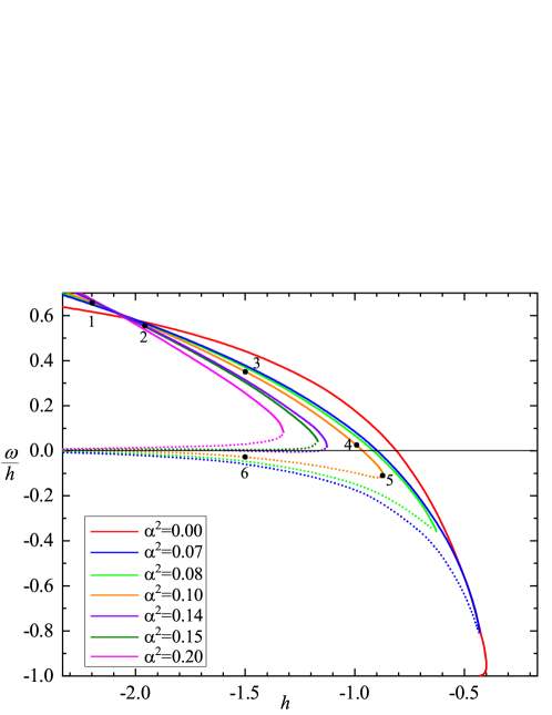
Figure 1: The normalized eigenvalue of the localized fermionic states is shown as a function of the Skyrmion-fermion coupling $h$ for several values of $\alpha^{2}$. The points 1-6 along the curve $\alpha^{2}=0.1$ correspond to the values of the parameters $\omega$ and $h$ for which profiles of the matter and metric fields are shown in Fig. 3. The point 2 corresponds to a configuration with ADM mass $M=0$ (cf. Fig. 2).

In the absence of gravity, the only parameter affecting the profile function of the backreacting Skyrmion is the Yukawa coupling. While the profile function always decreases monotonically from $F(0)=\pi$ to $F(\infty)=0$, the effective size of the configuration and the scaled mass are decreasing as the magnitude of the coupling becomes stronger. There are also other bound modes in the spectrum of the Dirac fermions localized on the Skyrmion in Minkowski spacetime [30, 31, 32], however, the normalizable bound mode crossing zero is unique.

The situation changes dramatically as gravity is added to this picture. There is a family of solutions depending continuously on two parameters, the Yukawa coupling constant $h$ and the eigenvalue of the Dirac operator $\omega$, for each particular value of the effective gravitational coupling $\alpha$. We recall that the appearance of a single zero crossing fermionic level is related to the underlying topology of the Skyrme field. Thus, we may expect that, as the self-gravitating configuration evolves towards the topologically trivial BM solution, this mode undergoes a certain transition.

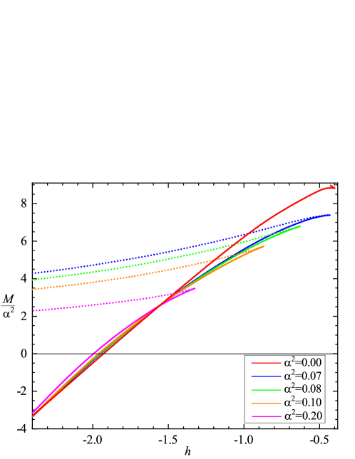
Figure 2: The ADM mass of the self-gravitating Skyrmion-fermion system is shown as a function of the Yukawa coupling $h$ for several values of $\alpha^{2}$.

Indeed, for any non-zero value of the gravitational coupling, the spherically symmetric fermionic mode localized on the Skyrmion is no longer linked to the negative continuum, as seen in Fig. 1. Instead, it arises at some particular value of the Yukawa coupling $h_{\text{max}}(\alpha)<h_{\text{cr}}$ with an scaled eigenvalue $\omega/h$ larger than the threshold value. Physically, this situation reflects the energy balance of the system of self-gravitating Skyrmions dressed by the fermions: the added gravitational interaction must be compensated by the force of the Yukawa interaction. Notably, the spectral flow of the fermionic Hamiltonian bifurcates at this point: as $h$ decreases below $h_{\text{max}}$, two branches arise as displayed in Fig. 1.

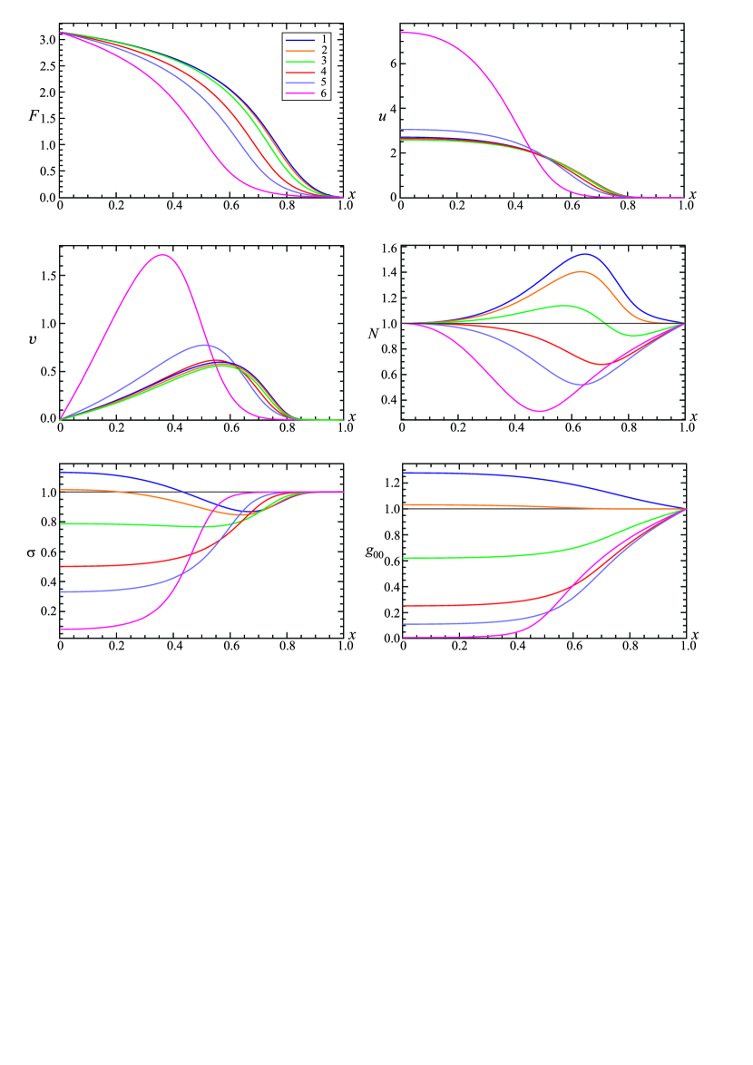
Figure 3: The field components of the self-gravitating Skyrmion-fermion system are shown as functions of the compactified radial coordinate $x$ for $\alpha^{2}=0.1$ for the points 1-6 in Fig. 1. The solution labeled as 2 corresponds to zero ADM mass.

We can understand qualitatively this pattern by analogy with the appearance of two branches of solutions for self-gravitating Skyrmions. The evolution of the configuration along one branch is related to the decrease of the Newton constant $G$, whereas the second branch may be considered as being obtained by decreasing the pion decay constant $f_{\pi}$. In both cases the effective gravitational coupling $\alpha$ is the same and the configuration remains in equilibrium for some particular value of the Yukawa coupling. By analogy with the case of the usual self-gravitating Skyrmions, we will refer to these branches of the spectral flow as the “Skyrmion branch” and the “BM branch”, respectively. To distinguish these branches visually, we plot them using solid (for the Skyrmion branch) and dotted (for the BM branch) lines in Figs. 1, 2, 4, and 5.

As $\alpha$ remains relatively weak, $\alpha^{2}\lesssim 0.14$, the Skyrmion branch of the spectral flow still crosses zero, and the BM branch slowly approaches zero from below, as seen in Fig. 1. Further increase of the gravitational coupling excludes the zero eigenvalue of the Dirac operator, and $\omega/h$ remains positive along both branches. On the BM branch, it then tends to zero from above, as the Yukawa coupling becomes stronger.

A rather intriguing observation is that the ADM mass of the coupled configuration becomes negative as $h$ decreases along the Skyrmion branch, as seen in Fig. 2. On the other hand, the ADM mass remains always positive along the BM branch.

In order to get a better understanding of this curious observation, let us now consider the pattern of evolution of the components of the coupled system (18)-(22). Fig. 3 presents the profile functions of the self-gravitating Skyrmion coupled to the localized fermionic mode for $\alpha^{2}=0.1$ and a set of values of the Yukawa coupling. Note that, as $h$ decreases below the critical value, labeled as the point 5 in Fig. 1, the size of the configuration on the Skyrmion branch increases. As the scaled eigenvalue $\omega/h$ crosses zero (the point 4) and becomes positive, the minimal values of the metric functions $N(r)$ and $\sigma(r)$ are increasing.

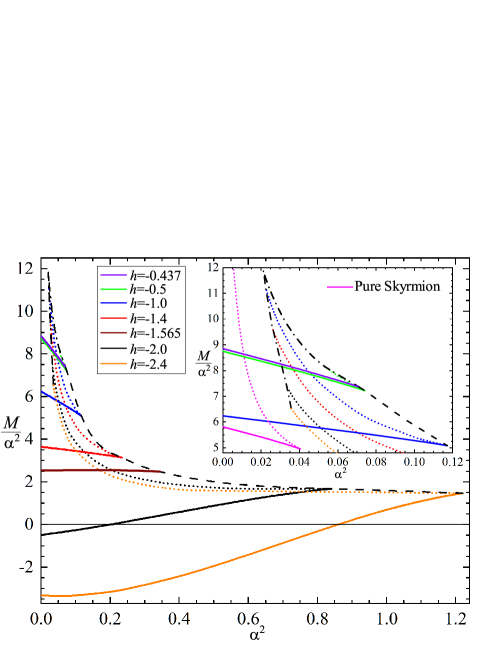
Figure 4: The ADM mass of the self-gravitating Skyrmion-fermion system is shown as a function of the effective gravitational coupling $\alpha^{2}$ for several values of $h$. The inset shows the behavior of the mass for small $\alpha^{2}$ in the neighbourhood of the maximum mass.

A further increase of the strength of the Skyrmion-fermion coupling for a fixed value of $\alpha$ yields a very unusual picture: the metric function $N(r)$ increases above unity in the interior of the Skyrmion, while it becomes less than unity in the outer region, as seen in Fig. 3 for the solution labeled by the point 3 in Fig. 1.

Notably, the ADM mass of the configuration becomes zero at some particular value of the Yukawa coupling, as seen in Fig. 2. At this critical point the metric component $g_{00}$ is nearly unity almost everywhere in space and the first derivative of the metric function $N$ at spatial infinity is vanishing, as displayed in Fig. 3.

As the Yukawa coupling becomes even stronger (the point 1 in Fig. 1), the metric function $N(r)$ is greater than unity, except at the boundaries, and the metric function $\sigma(r)$ becomes greater than unity in the inner region of the configuration. In contrast, the solution on the BM branch, labeled as the point 6 in Fig. 1, behaves as expected. The configuration becomes increasingly localized by the stronger gravitational attraction.

Fig. 4 displays the dependence of the ADM mass of the solutions on the effective gravitational coupling $\alpha^{2}$. As before, the solid lines correspond to the solutions on the Skyrmion branch, while the dotted lines represent the BM branch solutions. Both branches bifurcate at some maximal value $\alpha_{\text{max}}$, which increases as the absolute value of the Yukawa coupling $h$ becomes larger.

Unlike the self-gravitating Skyrmions in the decoupling limit $h=0$, the BM branches of the solutions with a localized fermionic mode do not extend all the way down to the limit $\alpha\to 0$, as seen in Fig. 4. For every BM branch, there is some limiting value of $\alpha_{\text{min}}(h)$ for which this branch terminates. Our numerical calculations indicate that there is a critical value of the Yukawa coupling $h\approx-0.79$ for which the ADM mass attains its maximum value $M/\alpha^{2}\approx 11.88$. This corresponds to the minimal value of the gravitational coupling $\alpha^{2}_{\text{min}}\approx 0.02$. Correspondingly, the increase or decrease in the strength of the Yukawa interaction increases the minimal value $\alpha_{\text{min}}(h)$, while the ADM mass of the corresponding limiting solutions decreases, as seen in Fig. 4. Here the dashed-dotted line corresponds to the sequence of limiting solutions on the BM branch which terminate at $\alpha_{\text{min}}$ as $h$ varies. In other words, the presence of the fermions prohibits the BM limit.

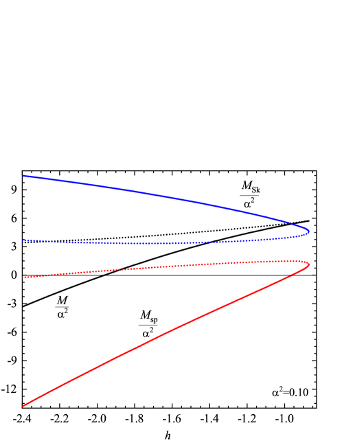
Figure 5: Contributions to the total ADM mass $M$ coming from the spinor ($M_{\text{sp}}$) and Skyrme ($M_{\text{Sk}}$) fields for different values of the Yukawa coupling and fixed $\alpha^{2}=0.1$. The black curve corresponds to the total ADM mass, cf. Fig. 2.

On the other hand, the domain of existence of the solutions is restricted by the bifurcation points, from which the Skyrmion and BM branches originate. These points are connected by the critical line (the dashed line in Fig. 4) which restricts the domain of existence of the solutions from above. This line starts at $\alpha^{2}\approx 0.07$ and $h\approx-0.437$ and extends up to the last calculated point at $\alpha^{2}\approx 1.22$ and $h=-2.4$. In turn, in the range $-0.4\lesssim h\lesssim-0.437$, BM branches are already absent, and there are only Skyrmion branches, which degenerate at $h\approx-0.4$ and $\alpha=0$ into one flat spacetime configuration, cf. Fig. 1. Curiously, for the fixed value of the Yukawa coupling $h=-1.565$ there is a certain family of configurations on the Skyrmion branch, whose mass remains approximately constant as $\alpha$ varies up to the bifurcation point (as seen in Fig. 4).

To get further insight, let us compare the contributions of the Skyrmion and fermionic fields to the total mass. In Fig. 5 we present the dependence of the corresponding quantities, evaluated by $M_{\text{Sk}}=\alpha^{2}\int dr\,r^{2}(T_{0}^{0})_{\text{Sk}}$ and $M_{\text{sp}}=\alpha^{2}\int dr\,r^{2}(T_{0}^{0})_{\text{sp}}$ (with $(T_{0}^{0})_{\text{Sk}}$ and $(T_{0}^{0})_{\text{sp}}$ given by Eqs. (28) and (31), respectively), and the total mass $M=M_{\text{Sk}}+M_{\text{sp}}$, on the Yukawa coupling. Clearly, the negative contribution of the fermionic mode becomes dominant on the Skyrmion branch, rendering the total mass negative. On the BM branch, on the other hand, both contributions remain positive for the Yukawa coupling $-2.25\lesssim h\lesssim-0.87$.

III.4 Violation of the null and weak energy conditions

The unexpected behavior of the solutions of the system (18)-(22) on the Skyrmion branch is related to the violation of the null and weak energy conditions, which state that the stress-energy tensor $T_{\mu\nu}$ satisfies, respectively, the inequalities

$$T_{\mu\nu}k^{\mu}k^{\nu}\geq 0\quad\text{and}\quad T_{\mu\nu}V^{\mu}V^{\nu}\geq 0$$

for any light-like vector $k^{\mu}$, $g_{\mu\nu}k^{\mu}k^{\nu}=0$, and for any timelike vector $V^{\mu}$, $g_{\mu\nu}V^{\mu}V^{\nu}>0$ (for a review, see e.g. Ref. [71]). Indeed, for the system (1) with the spherically symmetric Ansatz (11)-(13), the only nonvanishing components of the stress-energy tensors (9) and (10) are

$$\left(T^{0}_{0}\right)_{\text{Sk}}= N\frac{2\sin^{2}F+r^{2}}{2r^{2}}{F^{\prime}}^{2}+\frac{\sin^{2}F+2r^{2}}{2r^{4}}\sin^{2}F,$$ (28)

$$\left(T^{1}_{1}\right)_{\text{Sk}}= -N\frac{2\sin^{2}F+r^{2}}{2r^{2}}{F^{\prime}}^{2}+\frac{\sin^{2}F+2r^{2}}{2r^{4}}\sin^{2}F,$$ (29)

$$\left(T^{2}_{2}\right)_{\text{Sk}}= \left(T^{3}_{3}\right)_{\text{Sk}}=\frac{1}{2}N{F^{\prime}}^{2}-\frac{\sin^{4}F}{2r^{4}}$$ (30)

for the Skyrme field, and

$$\left(T^{0}_{0}\right)_{\text{sp}}= \omega\frac{u^{2}+v^{2}}{\sqrt{N}\sigma},$$ (31)

$$\left(T^{1}_{1}\right)_{\text{sp}}= 2uv\frac{hr\sin F+1}{r}+h\cos F\left(v^{2}-u^{2}\right)-\omega\frac{u^{2}+v^{2}}{\sqrt{N}\sigma},$$ (32)

$$\left(T^{2}_{2}\right)_{\text{sp}}= \left(T^{3}_{3}\right)_{\text{sp}}=-\frac{uv}{r}$$ (33)

for the fermion field. These components are written in a dimensionless form using the rescaling $T^{\mu}_{\nu}\to T^{\mu}_{\nu}/(a_{0}^{2}f_{\pi}^{4})$. Thus, the null/weak energy conditions for the self-gravitating coupled spherically symmetric Skyrmion-fermion system become

$$\begin{split}\epsilon+p\equiv&T^{0}_{0}-T^{1}_{1}=N\frac{2\sin^{2}F+r^{2}}{r^{2}}{F^{\prime}}^{2}\\ &+h\left[\cos F\left(u^{2}-v^{2}\right)-2uv\sin F\right]+2\omega\frac{u^{2}+v^{2}}{\sqrt{N}\sigma}-\frac{2uv}{r}\geq 0,\end{split}$$ (34)

where $\epsilon$ and $p$ are the energy density and radial pressure, respectively. In turn, the weak energy condition also implies $\epsilon\equiv T_{0}^{0}\geq 0$.

Evidently, the first term on the right-hand side of the expression (34) is related to the contribution of the Skyrme field. It is always positive, and a violation of the null/weak energy conditions can only be related to the contribution of the Dirac field.

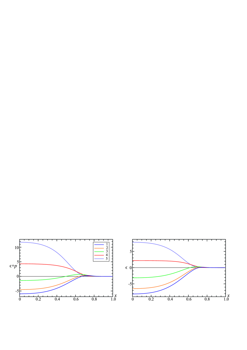
Figure 6: The function $\epsilon+p$ on the r.h.s. of the null/weak energy conditions (34) and the energy density $\epsilon$ for the solutions labeled as 1-5 in Fig. 1.

Indeed, in Fig. 6 we display the combination $\epsilon+p$ and the energy density $\epsilon$ for the configurations labeled by the points $1-5$ on the Skyrmion branch for $\alpha^{2}=0.1$ in Fig. 1. Clearly, the null/weak energy conditions become violated already for the solution labeled as the point $3$. Notice also that for all systems $1-5$ the pressure $p$ is always positive and the violation of the null/weak energy conditions is caused only by the negativeness of the energy density.

IV Conclusions

Static, spherically symmetric Skyrmions minimally coupled to gravity are the pioneering example of solitonic and hairy black hole solutions in General Relativity [14, 15, 16, 17, 18, 19]. The index theorem secures the existence of a bound fermionic mode localized on the self-gravitating Skyrmion. However, up to now, the effect of the presence of such a mode had not been considered. In this work, we have shown that the localization of the backreacting fermionic mode may have dramatic consequences, in particular, the energy conditions may be violated and regular self-gravitating asymptotically flat solutions with negative and zero ADM mass may emerge.

It may be of interest to compare our results to another well-known system, the self-gravitating non-Abelian monopole [11, 12, 13]. In both cases the flat space configurations represent spherically symmetric topological solitons in (3+1)-dimensions, and there is a spin-isospin fermionic mode localized on the soliton. However, the pattern of the dynamical evolution of the gravitating monopole and of the Skyrmion is different. While the branch of monopole solutions bifurcates with the extremal Reissner-Nordström black hole, the second branch of gravitating Skyrmions tends to the regular scaled BM solution. Further, the eigenvalue of the Dirac operator of the fermion mode localized on the monopole is always zero, it does not depend on the strength of the Yukawa coupling. This mode is fully absorbed into the interior of the black hole as the configuration approaches the Reissner-Nordström limit [60]. On the contrary, for the fermionic mode localized on the Skyrmion the variation of the Yukawa coupling gives rise to a spectral flow of the eigenvalues of the Dirac operator. The presence of this mode prevents the configuration from recovering the BM limit. On the other hand, the backreaction of the Dirac field on the spacetime geometry may produce coupled configurations with negative and zero ADM mass.

We note that the possibility of the emergence of a negative mass in General Relativity is being discussed for a long time [72, 73] (for some recent work, see, e.g., Refs. [74, 75, 76]). It has been pointed out that a region of negative energy density may collapse to a black hole with an unusual topology of the event horizon [77]. One might therefore wonder whether in the case of negative mass Skyrmion-fermion systems the possibility of forming a black hole of negative mass with Skyrmion-fermion hair might arise. This would be of particular interest, since previous attempts to obtain black holes with fermionic hair in (3+1)-dimensional asymptotically flat spacetime have failed [50, 51, 55, 78].

Finally, we note that it has already been suggested that Skyrmions may have technological significance in the future, providing fuel for the engines of Star Trek starships [79]. Our results indicate that Skyrmions may have even far wider important ramifications, providing an example of anti-gravitating matter.

References

- [1] G. ’t Hooft, Nucl. Phys. B 79, 276 (1974).
- [2] A. M. Polyakov, JETP Lett. 20, 194 (1974).
- [3] T. H. R. Skyrme, Proc. Roy. Soc. Lond. A 260, 127 (1961).
- [4] T. H. R. Skyrme, Nucl. Phys. 31, 556 (1962).
- [5] L. D. Faddeev, Print-75-0570 (IAS, PRINCETON).
- [6] L. D. Faddeev and A. J. Niemi, Nature 387, 58 (1997).
- [7] N. S. Manton and P. Sutcliffe, Topological solitons (Cambridge University Press, 2004).
- [8] Y. M. Shnir, Topological and Non-Topological Solitons in Scalar Field Theories (Cambridge University Press, 2018).
- [9] M. S. Volkov and D. V. Gal’tsov, Phys. Rept. 319, 1 (1999).
- [10] M. S. Volkov, “Hairy black holes in the XX-th and XXI-st centuries”, Proceedings of the Fourteenth Marcel Grossmann Meeting, eds M. Bianchi, R. Jantzen and R. Ruffini, World Scientific, pp. 1779-1798 (2017).
- [11] K. M. Lee, V. P. Nair, and E. J. Weinberg, Phys. Rev. D 45, 2751 (1992).
- [12] P. Breitenlohner, P. Forgacs, and D. Maison, Nucl. Phys. B 383, 357 (1992).
- [13] P. Breitenlohner, P. Forgacs, and D. Maison, Nucl. Phys. B 442, 126 (1995).
- [14] H. Luckock and I. Moss, Phys. Lett. B 176, 341 (1986).
- [15] N. K. Glendenning, T. Kodama, and F. R. Klinkhamer, Phys. Rev. D 38, 3226 (1988).
- [16] S. Droz, M. Heusler, and N. Straumann, Phys. Lett. B 268, 371 (1991).
- [17] M. Heusler, S. Droz, and N. Straumann, Phys. Lett. B 271, 61 (1991).
- [18] P. Bizon and T. Chmaj, Phys. Lett. B 297, 55 (1992).
- [19] M. Heusler, N. Straumann, and Z. h. Zhou, Helv. Phys. Acta 66, 614 (1993).
- [20] M. F. Atiyah, V. K. Patodi, and I. M. Singer, Math. Proc. Cambridge Phil. Soc. 77, 43 (1975).
- [21] C. Caroli, P.G. de Gennes, and J. Matricon, Phys. Lett.9, 307 (1964).
- [22] R. Jackiw and C. Rebbi, Phys. Rev. D 13, 3398 (1976).
- [23] R. F. Dashen, B. Hasslacher, and A. Neveu, Phys. Rev. D 10, 4130 (1974).
- [24] Y. Z. Chu and T. Vachaspati, Phys. Rev. D 77, 025006 (2008).
- [25] D. Stojkovic, Phys. Rev. D 63, 025010 (2001).
- [26] V. A. Rubakov, Nucl. Phys. B 203, 311 (1982).
- [27] C. G. Callan, Jr., Phys. Rev. D 26, 2058 (1982).
- [28] C. R. Nohl, Phys. Rev. D 12, 1840 (1975).
- [29] J. Boguta and J. Kunz, Phys. Lett. B 154, 407 (1985).
- [30] J. R. Hiller and T. F. Jordan, Phys. Rev. D 34, 1176 (1986).
- [31] S. Kahana and G. Ripka, Nucl. Phys. A 429, 462 (1984).
- [32] A. P. Balachandran and S. Vaidya, Int. J. Mod. Phys. A 14, 445 (1999).
- [33] E. Witten, Nucl. Phys. B 249, 557 (1985).
- [34] R. Jackiw and P. Rossi, Nucl. Phys. B 190, 681 (1981).
- [35] V. A. Gani, V. G. Ksenzov, and A. E. Kudryavtsev, Phys. Atom. Nucl. 73, 1889 (2010).
- [36] A. Amado and A. Mohammadi, Eur. Phys. J. C 77, 465 (2017).
- [37] V. Klimashonok, I. Perapechka, and Y. Shnir, Phys. Rev. D 100, 105003 (2019).
- [38] I. Perapechka and Y. Shnir, Phys. Rev. D 101, 021701 (2020).
- [39] I. Perapechka, N. Sawado, and Y. Shnir, JHEP 10, 081 (2018).
- [40] I. Perapechka and Y. Shnir, Phys. Rev. D 99, 125001 (2019).
- [41] J. G. F. Campos and A. Mohammadi, JHEP 08, 180 (2022).
- [42] V. A. Gani, A. Gorina, I. Perapechka, and Y. Shnir, Eur. Phys. J. C 82, 757 (2022).
- [43] D. Bazeia, J. G. F. Campos, and A. Mohammadi, JHEP 12, 085 (2022).
- [44] D. Saadatmand and H. Weigel, Phys. Rev. D 107, 036006 (2023).
- [45] H. Weigel and D. Saadatmand, [arXiv:2311.14437 [hep-th]]
- [46] A. H. Taub, Phys. Rev. 51, 512 (1937).
- [47] M. S. Volkov, Phys. Lett. B 334, 40 (1994).
- [48] C. Armendariz-Picon and P. B. Greene, Gen. Rel. Grav. 35, 1637 (2003).
- [49] Y. F. Cai and J. Wang, Class. Quant. Grav. 25, 165014 (2008).
- [50] F. Finster, J. Smoller, and S. T. Yau, Phys. Rev. D 59, 104020 (1999).
- [51] C. Herdeiro, I. Perapechka, E. Radu, and Y. Shnir, Phys. Lett. B 797, 134845 (2019).
- [52] V. Dzhunushaliev and V. Folomeev, Phys. Rev. D 99, 084030 (2019).
- [53] V. Dzhunushaliev and V. Folomeev, Phys. Rev. D 99, 104066 (2019).
- [54] J. L. Blázquez-Salcedo and C. Knoll, Eur. Phys. J. C 80, 174 (2020).
- [55] C. Herdeiro, I. Perapechka, E. Radu, and Y. Shnir, Phys. Lett. B 824, 136811 (2022).
- [56] J. L. Blázquez-Salcedo, C. Knoll, and E. Radu, Phys. Rev. Lett. 126, 101102 (2021).
- [57] S. Bolokhov, K. Bronnikov, S. Krasnikov, and M. Skvortsova, Grav. Cosmol. 27, 401 (2021).
- [58] R. A. Konoplya and A. Zhidenko, Phys. Rev. Lett. 128, no.9, 091104 (2022).
- [59] T. D. Lee and Y. Pang, Phys. Rev. D 35, 3678 (1987).
- [60] V. Dzhunushaliev, V. Folomeev, and Y. Shnir, Phys. Rev. D 108, 065005 (2023).
- [61] S. R. Dolan and D. Dempsey, Class. Quant. Grav. 32, 184001 (2015).
- [62] T. Eguchi, P. B. Gilkey, and A. J. Hanson, Phys. Rept. 66, 213 (1980).
- [63] M. Gell-Mann and M. Levy, Nuovo Cim. 16, 705 (1960).
- [64] S. Krusch, J. Phys. A 36, 8141 (2003).
- [65] Y. Shnir, Phys. Scripta 67, 361 (2003).
- [66] R. Jackiw and C. Rebbi, Phys. Rev. Lett. 36, 1116 (1976).
- [67] G. S. Adkins, C. R. Nappi, and E. Witten, Nucl. Phys. B 228, 552 (1983).
- [68] N. S. Manton and S. W. Wood, Phys. Rev. D 74, 125017 (2006).
-
[69]
N.I.M. Gould, J.A. Scott, Y. Hu,
ACM Trans. Math. Softw. 33, 10 (2007);
O. Schenk, K. Gartner, Future Gener. Comput. Syst. 20, 475 (2004). - [70] J. Kunz, I. Perapechka, and Y. Shnir, JHEP 07, 109 (2019).
- [71] V. A. Rubakov, Phys. Usp. 57, 128 (2014).
- [72] H. Bondi, Rev. Mod. Phys. 29, 423 (1957).
- [73] D. Harari and C. Lousto, Phys. Rev. D 42, 2626 (1990).
- [74] S. Mbarek and M. B. Paranjape, Phys. Rev. D 90, 101502 (2014).
- [75] J. S. Farnes, Astron. Astrophys. 620, A92 (2018).
- [76] C. H. Hao, L. X. Huang, X. Su, and Y. Q. Wang, [arXiv:2312.03800 [gr-qc]].
- [77] R. B. Mann, Class. Quant. Grav. 14, 2927 (1997).
- [78] J. l. Jing, Phys. Rev. D 70, 065004 (2004).
- [79] S. Krusch and P. Sutcliffe, J. Phys. A 37, 9037 (2004).