Generalization Error Curves for Analytic Spectral Algorithms under Power-law Decay

Abstract

The generalization error curve of certain kernel regression method aims at determining the exact order of generalization error with various source condition, noise level and choice of the regularization parameter rather than the minimax rate. In this work, under mild assumptions, we rigorously provide a full characterization of the generalization error curves of the kernel gradient descent method (and a large class of analytic spectral algorithms) in kernel regression. Consequently, we could sharpen the near inconsistency of kernel interpolation and clarify the saturation effects of kernel regression algorithms with higher qualification, etc. Thanks to the neural tangent kernel theory, these results greatly improve our understanding of the generalization behavior of training the wide neural networks. A novel technical contribution, the analytic functional argument, might be of independent interest.

Keywords reproducing kernel Hilbert space, spectral algorithm, gradient descent, analytic functional calculus

1 Introduction

The neural tangent kernel (NTK) theory (Jacot et al., 2018), which shows that the gradient kernel regression approximates the over-parametrized neural network trained by gradient descent well  (Jacot et al., 2018; Allen-Zhu et al., 2019; Lee et al., 2019), brings us a natural surrogate to understand the generalization behavior of the neural networks in certain circumstances. This surrogate has led to recent renaissance of the study of kernel methods. For example, one would ask whether overfitting could harm the generalization (Bartlett et al., 2020), how the smoothness of the underlying regression function would affect the generalization error (Li et al., 2023), or if one can determine the lower bound of the generalization error at a specific function? All these problems can be answered by the generalization error curve which aims at determining the exact generalization error of a certain kernel regression method with respect to the kernel, the regression function, the noise level and the choice of the regularization parameter. It is clear that such a generalization error curve would provide a comprehensive picture of the generalization ability of the corresponding kernel regression method  (Bordelon et al., 2020; Cui et al., 2021; Li et al., 2023).

Although there have been extensive works on the generalization errors of kernel regression, most of them focused on the optimal rate of convergence under the minimax framework. For example, Caponnetto and De Vito (2007) showed with a proper choice of the regularization parameter, kernel ridge regression (KRR) can achieve the minimax optimal rate of convergence. Being a special case, KRR falls into a large class of kernel methods often referred to as spectral algorithms (Rosasco et al., 2005; Gerfo et al., 2008). For general spectral algorithms, subsequent works (e.g., Blanchard and Mücke (2018); Lin et al. (2018)) proved similar optimality results. We refer the reader to Subsection 1.1 for more details. However, these works are not sufficient to answer the aforementioned problems motivated from the studies in neural networks, since they only considered the method-dependent upper bound and the method-independent minimax lower bound of the generalization error. In addition, most of them focused mainly on the rate of convergence and ignored the constant factors. Therefore, these traditional results are not enough to provide a comprehensive picture of the generalization error of kernel methods.

Going beyond the traditional results, several recent works attempt to describe the generalization error curve of kernel ridge regression (KRR). With some heuristic arguments, Bordelon et al. (2020); Cui et al. (2021) derived the generalization error curve of KRR under certain restrictive assumptions. Under mild assumptions, Li et al. (2023) first rigorously characterized the generalization error curve of KRR in terms of asymptotic convergence rate. They show an exact bias-variance trade-off U-shaped curve for the generalization error of KRR with respect to the choice of regularization parameter. Since the neural networks are often trained by the gradient descent, it is of great interest to further study the generalization error curves of the gradient descent kernel regression. To the best of our knowledge, few attention is made on this aspect.

In this paper, we study the generalization error curves of a large class of analytic spectral algorithms, including the kernel gradient method. To be precise, let $\rho$ be a probability distribution on $\mathcal{X}\times\mathbb{R}$ and $f^{*}$ be the unknown regression function (Andreas Christmann, 2008), namely the conditional expectation $f^{*}(x)=\mathbb{E}_{\rho}(y|x)$. Given $n$ i.i.d. samples $\{(x_{i},y_{i})\}_{i=1}^{n}$, let $\hat{f}_{\lambda}$ be the estimator given by a spectral algorithm with regularization parameter $\lambda=\lambda(n)>0$. Then, our result shows that for $\lambda$ in a reasonable range,

$$\mathbb{E}\left[\norm{\hat{f}_{\lambda}-f^{*}}_{L^{2}}^{2}~{}\Big{|}~{}X\right]=(1+o_{\mathbb{P}}(1))\left(\mathcal{R}_{\varphi}^{2}(\lambda;f^{*})+\frac{\sigma^{2}}{n}\mathcal{N}_{2,\varphi}(\lambda)\right),$$

where the conditional expectation is taken with respect to the training sample $X=(x_{1},\dots,x_{n})$, $\sigma^{2}$ is the variance of the noise, $\mathcal{R}_{\varphi}^{2}(\lambda;f^{*})$ and $\mathcal{N}_{2,\varphi}(\lambda)$ are two deterministic quantities (see (28) and (29)) corresponding to the bias and the variance respectively, and $\varphi$ is the filter function defining the spectral algorithm (see (19)). Moreover, if $\lambda$ does not lie in the reasonable range, we also show that the generalization error is lower bounded by nearly a constant. The assumptions made in this paper are also mild and are satisfied for many RKHSs and spectral algorithms. We refer to Section 3 for a complete statement for our main result.

With the exact $1+o_{\mathbb{P}}(1)$ form, our result characterizes exactly and completely the generalization error for a large class of analytic spectral algorithms. In particular, it shows a solid U-shaped bias-variance trade-off curve that the bias decreases while the variance increases as the regularization strength $\lambda$ decreases, where the optimal point corresponds to the minimax optimal rate of convergence. The result also shows that when the regularization is too weak, the overfitting method can not generalize, emphasizing the necessity of regularization. Moreover, our result also expose a high-order saturation effect of some specific spectral algorithms. Our result would greatly improve the understanding of the generalization behavior of spectral algorithms and the wide neural networks.

Last but not the least, the novel application of the “analytic functional argument” in deriving sharp estimations for spectral algorithms might be of independent interest and worth of further investigations.

1.1 Related works

Optimality of kernel methods

There are a large number of works studying the optimal rates of kernel ridge regression and also spectral algorithms. The classical work (Caponnetto and De Vito, 2007) proved the minimax optimality of KRR when the regression lies in the RKHS; subsequent works (Steinwart et al., 2009; Fischer and Steinwart, 2020; Zhang et al., 2023) further extend the result to the misspecified cases when the regression function does not lie in the RKHS. Zhang and Yu (2005) and Yao et al. (2007) considered the kernel gradient method and proved consistency and fast rates of convergence respectively. The general spectral algorithms are first introduced Bauer et al. (2007) and then studied extensive in the follow-up works (Gerfo et al., 2008; Rosasco et al., 2005), but the eigenvalue decay (see Assumption 1) of the kernel was not considered so the rates are not optimal. When certain restrictive conditions, Caponnetto (2006) proved the minimax optimality of the spectral algorithms. More recently, a sequence of works further extend the result to more general cases (e.g., Blanchard and Mücke (2018); Lin et al. (2018)). In addition, the very recent work (Zhang et al., 2023) showed the optimality for the misspecified cases even when the regression function is unbounded. We also refer to Table 1 in Zhang et al. (2023) for a summary of the results. However, as discussed above, these results only focused on the upper bounds and are not enough to provide the exact generalization error curve.

Recent advances in kernel ridge regression

Focusing particularly on KRR, a recent line of work provide further results on its generalization. Some works (Rakhlin and Zhai, 2018; Buchholz, 2022; Beaglehole et al., 2022; Li et al., 2023) studied kernel ridgeless regression, which is the limiting case of KRR as the regularization goes to zero, and proved that it can not generalize. Using a restrictive Gaussian design assumption and also some non-rigorous arguments, Bordelon et al. (2020); Cui et al. (2021) derived the generalization error curve of KRR and Mallinar et al. (2022) studied further the interpolation regime. For rigorous results, Li et al. (2023) proved the generalization error curve with asymptotic rates in the form of $\Theta_{\mathbb{P}}(n^{-r})$, but the hidden constant factors are not tracked.

Kernel regression in the high-dimensional limit

There is also a line of works studying the generalization of kernel regression in the high-dimensional limit when the dimension of the input space $d$ diverges with $n$. For example, in the high-dimensional setting, Liang and Rakhlin (2020) showed that kernel interpolation can generalize; Ghorbani et al. (2020); Ghosh et al. (2021); Liu et al. (2021); Lu et al. (2023) studied the generalization of kernel ridge regression and kernel gradient method. However, we would like to emphasize that their results could be substantially different from ours since the setting is different. Moreover, the high dimensionality in their setting actually makes the problem easier since the kernel can now be linearizing and the well-established random matrix theory can be applied, which is not the case in our setting.

2 Preliminaries

2.1 Reproducing kernel Hilbert space

Let a compact metric space $\mathcal{X}$ be the space of input and $\mathcal{Y}\subseteq\mathbb{R}$ be the space of output. Let $\rho$ be the unknown probability measure supported on $\mathcal{X}\times\mathcal{Y}$ and $\mu$ be the marginal probability measure of $\rho$ on $\mathcal{X}$. Denote by $L^{2}=L^{2}(\mathcal{X},\differential\mu)$ the space of (complex-valued) square integrable functions on $\mathcal{X}$. Assume that $\mathbb{E}_{(x,y)\sim\rho}(y^{2})<\infty$, let the conditional expectation

$$f^{*}(x)=\mathbb{E}_{\rho}(y\mid x)=\int_{\mathcal{Y}}y\differential\rho(y|x)\in L^{2}$$ (1)

be the regression function. We fix a continuous positive definite kernel $k:\mathcal{X}\times\mathcal{X}\to\mathbb{C}$ over $\mathcal{X}$ and let $\mathcal{H}$ be the (complex) separable reproducing kernel Hilbert space (RKHS) associated with $k$. Note that we adopt the convention that inner product is linear in the second component and conjugate linear in the first component, that is, $\left\langle{f,g}\right\rangle_{L^{2}}=\int_{\mathcal{X}}\overline{f(x)}g(x)\differential x$ and $\left\langle{k(x,\cdot),f}\right\rangle_{\mathcal{H}}=f(x)$ for $f\in\mathcal{H}$. Since $\mathcal{X}$ is compact and $k$ is continuous, we have $\sup_{x\in\mathcal{X}}k(x,x)\leq\kappa^{2}<\infty$. Consequently, we have the natural inclusion $S_{k}:\mathcal{H}\to L^{2}$ which is Hilbert-Schmidt (Andreas Christmann, 2008; Steinwart and Scovel, 2012). Denote by $S_{k}^{*}:L^{2}\to\mathcal{H}$ the adjoint operator of $S_{k}$. Then, $T=S_{k}S_{k}^{*}:L^{2}\to L^{2}$ defines a integral operator

$$(Tf)(x)=\int_{\mathcal{X}}\overline{k(x,x^{\prime})}f(x^{\prime})\differential\mu(x^{\prime}).$$ (2)

Moreover, it is well known (Caponnetto and De Vito, 2007; Steinwart and Scovel, 2012) that $T$ is a self-adjoint, positive and trace class operator that the trace norm $\norm{T}_{1}\leq\kappa^{2}$. Focusing only on the infinite dimensional case that $T$ is not of finite rank, we have the spectral decomposition

$$T=\sum_{m=1}^{\infty}\mu_{m}P_{V_{m}},$$ (3)

where $(\mu_{m})_{m\geq 1}$ is the decreasing sequence of the distinct positive eigenvalues of $T$ and $P_{V_{m}}$ is the projection onto the eigenspace $V_{m}$ associated with $\mu_{m}$. Denote by $d_{m}=\dim V_{m}$ the multiplicity of $\mu_{m}$. Let us further choose an orthonormal basis $\{e_{m,l}\}_{l=1}^{d_{m}}$ for each $V_{m}$, where each $e_{m,l}$ is the continuous representative among the $\mu$-equivalent class. Then, $\{e_{m,l}\}$ forms an orthonormal basis of $\overline{\operatorname{Ran}S_{k}}=(\operatorname{Ker}S_{k}^{*})^{\perp}\subseteq L^{2}$ and $\{\mu_{m}^{1/2}e_{m,l}\}$ forms an orthonormal basis of $\overline{\operatorname{Ran}S_{k}^{*}}=(\operatorname{Ker}S_{k})^{\perp}=\mathcal{H}$, where we notice that $S_{k}$ is injective since the support of $\mu$ is $\mathcal{X}$. Finally, the Mercer’s theorem (Andreas Christmann, 2008; Steinwart and Scovel, 2012) yields that

$$k(x,x^{\prime})=\sum_{m=1}^{\infty}\mu_{m}\sum_{l=1}^{d_{m}}\overline{e_{m,l}(x)}e_{m,l}(x^{\prime}),$$ (4)

where the summation converges absolutely and uniformly. To be in line with the previous literature, we denote by $(\lambda_{j})_{j\geq 1}$ the eigenvalues of $T$ counting multiplicities and, with a little abuse of notation, denote by $e_{j}$ the corresponding eigenfunction. Then, we introduce the following assumption on the eigenvalues of $T$, which is commonly considered in the previous literature  (Caponnetto and De Vito, 2007; Fischer and Steinwart, 2020; Li et al., 2023).

Assumption 1 (Eigenvalue decay).

There are some $\beta>1$ and constants $c_{\mathrm{eig}},C_{\mathrm{eig}}>0$ such that

$$c_{\mathrm{eig}}j^{-\beta}\leq\lambda_{j}\leq C_{\mathrm{eig}}j^{-\beta},\quad j\geq 1,$$ (5)

or equivalently,

$$\#\{i:\lambda_{i}\geq\lambda\}=\sum_{m:\mu_{m}\geq\lambda}d_{m}=\Theta(\lambda^{-1/\beta}),\mbox{\quad as\quad}\lambda\to 0.$$ (6)

where $(\lambda_{j})_{j\geq 1}$ are the eigenvalues (counting multiplicities) of the integral operator $T$ and $\{\mu_{m}\}_{m\geq 1}$ are the distinct ones defined in (3).

Remark 2.1.

The equivalence of (5) and (6) is elementary and a proof can be found in Proposition A.1. (6) allows us to deal with some less explicit cases. For example, if we have $\sum_{k=1}^{m}d_{k}\asymp m^{\gamma}$ for some $\gamma\geq 1$, then $\lambda_{j}\asymp j^{-\beta}$ is just equivalent to $\mu_{m}\asymp m^{-\gamma\beta}$.

Assumption 1 is satisfied by many commonly used kernels, such as Laplacian kernel, Matérn kernel and neural tangent kernel etc. This assumption on the eigenvalues characterizes the smoothness of the functions in the RKHS and larger $\beta$ implies better smoothness. We also remark that since $T$ is trace-class, $(\lambda_{j})_{j\geq 1}$ is summable so the requirement $\beta>1$ is necessary. Assumption 1 is also closely connected to the effective dimension or capacity condition of the RKHS in the previous literature (Caponnetto and De Vito, 2007). Later, with a spectral algorithm $\varphi$, we will introduce generalized $\varphi$-effective dimension that characterizes the variance of the method, see (29).

Interpolation spaces

We need to further introduce the interpolation spaces (Steinwart and Scovel, 2012) to state our results. For $p\geq 0$, we define the fractional power $T^{p}:L^{2}\to L^{2}$ by

$$T^{p}=\sum_{m=1}^{\infty}\mu_{m}^{p}P_{V_{m}}=\sum_{m=1}^{\infty}\mu_{m}^{p}\sum_{l=1}^{d_{m}}\left\langle{e_{m,l},\cdot}\right\rangle_{L^{2}}e_{m,l}.$$ (7)

Then, we can introduce the interpolation space $[\mathcal{H}]^{s}$ by

$$[\mathcal{H}]^{s}=\operatorname{Ran}T^{s/2}=\left\{f=\sum_{m=1}^{\infty}\mu_{m}^{s/2}\sum_{l=1}^{d_{m}}a_{m,l}e_{m,l}~{}\Big{|}~{}\sum_{m=1}^{\infty}\sum_{l=1}^{d_{m}}\absolutevalue{a_{m,l}}^{2}<\infty\right\}\subseteq L^{2}.$$ (8)

For $f,g\in[\mathcal{H}]^{s}$ with coefficients $(a_{m,l})$ and $(b_{m,l})$ respectively, we define the inner product in $[\mathcal{H}]^{s}$ by

$$\left\langle{f,g}\right\rangle_{[\mathcal{H}]^{s}}=\sum_{m=1}^{\infty}\sum_{l=1}^{d_{m}}\overline{a_{m,l}}b_{m,l}=\left\langle{T^{-\frac{s}{2}}f,T^{-\frac{s}{2}}g}\right\rangle_{L^{2}}.$$ (9)

Then, it is easy to see that $[\mathcal{H}]^{s}$ is a separable Hilbert space with an orthogonal basis $\{\mu_{m}^{s/2}e_{m,l}:~{}m\geq 1,~{}1\leq l\leq d_{m}\}$. In particular, we have $[\mathcal{H}]^{0}\subseteq L^{2}$ and also $[\mathcal{H}]^{1}=\mathcal{H}$. We also have natural inclusions $[\mathcal{H}]^{s}\subseteq[\mathcal{H}]^{t}$ for $s\geq t$ and the inclusion is compact if $s>t$. Moreover, the restriction of $T$ (and also $T^{p}$) on $[\mathcal{H}]^{s}$ is also a bounded operator with the same spectra, so we will still denote it by $T$ (and also $T^{p}$) for simplicity.

Regular RKHS

To derive the tightest possible learning rate, we need to characterize the regularity of the functions in the RKHS to the greatest extent. Since $V_{m}$ is a finite dimensional space of $L^{2}$ and also $\mathcal{H}$, it is a reproducing kernel Hilbert space with respect to $\left\langle{\cdot,\cdot}\right\rangle_{L^{2}}$ and its reproducing kernel $k_{m}$ is determined uniquely by

$$\left\langle{k_{m}(x,\cdot),f}\right\rangle_{L^{2}}=\int_{\mathcal{X}}\overline{k_{m}(x,x^{\prime})}f(x^{\prime})\differential\mu(x^{\prime})=f(x).$$ (10)

Choosing an orthonormal basis $\{e_{m,l}\}_{l=1}^{d_{m}}$, we have explicitly

$$k_{m}(x,x^{\prime})=\sum_{l=1}^{d_{m}}\overline{e_{m,l}(x)}e_{m,l}(x^{\prime}),$$ (11)

which is invariant of the choice of the basis. It is also easy to see that

$$k(x,x^{\prime})=\sum_{m=1}^{\infty}\mu_{m}k_{m}(x,x^{\prime}).$$

In this paper, we introduce the following condition of regular RKHS:

Assumption 2 (Regular RKHS).

There is some constant $M>0$ such that

$$\sup_{x\in\mathcal{X}}\sum_{m=1}^{N}k_{m}(x,x)=\sup_{x\in\mathcal{X}}\sum_{m=1}^{N}\sum_{l=1}^{d_{m}}\absolutevalue{e_{m,l}(x)}^{2}\leq M\sum_{m=1}^{N}d_{m},\quad\forall N\geq 1,$$ (12)

In this case, we call this RKHS (together with the underlying distribution $\mu$) is regular.

It is obvious that if the eigenfunctions are uniformly bounded, that is, $\sup_{x\in\mathcal{X}}\absolutevalue{e_{m,l}(x)}^{2}\leq M$, then the RKHS is regular. Moreover, there are some more cases that the RKHS is regular, so we believe that it is a rather general assumption.

Example 2.1 (Shift-invariant periodic kernels).

Let $\mathcal{X}=\mathbb{T}^{d}=[-\pi,\pi)^{d}$ be the $d$-dimensional torus and $\mu$ be the uniform measure on $\mathbb{T}^{d}$. Consider a shift-invariant kernel satisfying $k(x,y)=h(x-y)$, where $h$ is a function defined on $\mathbb{T}^{d}$. Then, it is easy to show that the Fourier basis $\{\phi_{\bm{m}}=e^{i\left\langle{\bm{m},x}\right\rangle},~{}m\in\mathbb{Z}^{d}\}$ gives an orthonormal set of eigenfunctions of $T$. Consequently, it is regular since the basis is uniformly bounded. Moreover, if the corresponding eigenvalues satisfy $\lambda_{\bm{m}}\asymp(1+\norm{\bm{m}}_{2}^{2})^{-\alpha}$, then the corresponding RKHS is $\mathcal{H}\cong H^{\alpha}(\mathbb{T}^{d})$, the Sobolev space on $\mathbb{T}^{d}$, and also $[\mathcal{H}]^{s}\cong H^{s\alpha}(\mathbb{T}^{d})$.

Example 2.2 (Dot-product kernel on the sphere).

Let $\mathcal{X}=\mathbb{S}^{d}$ be the $d$-dimensional sphere and $\mu$ be the uniform measure on $\mathbb{S}^{d}$. Consider a dot-product kernel satisfying $k(x,y)=h(\left\langle{x,y}\right\rangle)$, where $h$ is a function on $[-1,1]$. Then, the Funk-Hecke formula (Dai and Xu, 2013) shows that the spherical harmonics $\{Y_{m,l}~{}m\geq 1,~{}1\leq l\leq d_{m}\}$ consists of an orthonormal set of eigenfunctions of $T$, where $\{Y_{m,l}~{}1\leq l\leq d_{m}\}$ are order-$m$ homogeneous harmonic polynomials and $d_{m}=\binom{m+d}{m}-\binom{m-2+d}{m-2}\asymp m^{d-1}$. Using the theory of spherical harmonics, we can show that this RKHS is regular, see Subsection B.1.1.

Example 2.3 (Dot-product kernel on the ball).

Now, let us consider the $d$-dimensional unit ball $\mathcal{X}=\mathbb{B}^{d}=\{x\in\mathbb{R}^{d+1}:\norm{x}\leq 1\}$ with $\mu$ be proportional to the classical weight $p(x)=(1-\norm{x}^{2})^{-1/2}$. Consider still a dot-product kernel $k$. Then, an analog of the Funk-Hecke formula on the ball Dai and Xu (2013, Section 11) shows that the space $V_{m}^{d}$ of orthogonal polynomials of degree exactly $m$ is an eigenspace associated with the same eigenvalue of $T$ and $\dim V_{m}^{d}=\binom{m+d-1}{m}\asymp m^{d-1}$. Similar to the spherical case, we can show that this RKHS is regular, see Subsection B.1.2.

In previous literature (Steinwart et al., 2009; Fischer and Steinwart, 2020; Zhang et al., 2023), the following $L^{\infty}$-embedding property is introduced to characterize the regularity of the RKHS. We say $\mathcal{H}$ has an embedding property of order $\alpha\in(0,1]$ if $[\mathcal{H}]^{\alpha}$ can be continuously embedded into $L^{\infty}(\mathcal{X},\differential\mu)$, that is, the operator norm

$$M_{\alpha}\coloneqq\norm{[\mathcal{H}]^{\alpha}\hookrightarrow L^{\infty}(\mathcal{X},\mu)}<\infty.$$ (13)

Then, we define the embedding index by $\alpha_{0}=\inf\left\{\alpha:M_{\alpha}<\infty\right\}$. It is obvious that $\alpha\leq 1$ because

$$\sup_{x\in\mathcal{X}}\absolutevalue{f(x)}=\sup_{x\in\mathcal{X}}\left\langle{k(x,\cdot),f}\right\rangle_{\mathcal{H}}\leq\norm{k(x,\cdot)}_{\mathcal{H}}\norm{f}_{\mathcal{H}}\leq\kappa\norm{f}_{\mathcal{H}},$$

and it is also shown in Fischer and Steinwart (2020, Lemma 10) that $\alpha_{0}\geq\beta$. To obtain sharp concentrations, previous works (Zhang et al., 2023; Li et al., 2023) assume that $\alpha_{0}=\beta$. Here we show that this embedding index condition is satisfied by the regular RKHS.

Proposition 2.2.

Under Assumption 1 and Assumption 2, the embedding index is $\alpha_{0}=1/\beta$.

Moreover, we remark that the embedding index condition only makes sense for the eigenvalues with power-law decay, while the regular RKHS condition can also be considered for more general decays. In fact, the regular RKHS condition essentially considers the eigenfunctions rather than the eigenvalues.

2.2 Spectral algorithm

Let $Z=\{(x_{i},y_{i})\}_{i=1}^{n}\subseteq\mathcal{X}\times\mathcal{Y}$ be a set of training sample drawn i.i.d. from $\rho$. We also denote by $X=(x_{1},\dots,x_{n})$ the collection of sample inputs. To introduce the spectral algorithm, we first introduce some auxiliary notations. Denote by $k_{x}=k(x,\cdot)\in\mathcal{H}$. Let $K_{x}:\mathbb{R}\to\mathcal{H}$ be given by $K_{x}y=yk_{x}$, whose adjoint $K_{x}^{*}:\mathcal{H}\to\mathbb{R}$ is given by $K_{x}^{*}f=\left\langle{k_{x},f}\right\rangle_{\mathcal{H}}=f(x)$. Moreover, we denote by $T_{x}=K_{x}K_{x}^{*}:\mathcal{H}\to\mathcal{H}$ and

$$T_{X}=\frac{1}{n}\sum_{i=1}^{n}T_{x_{i}}.$$ (14)

Here we notice that since $k(x,x)\leq\kappa^{2}$, we have $\norm{T_{X}}\leq\kappa^{2}$. We also define the sample basis function

$$\hat{g}_{Z}=\frac{1}{n}\sum_{i=1}^{n}K_{x_{i}}y_{i}=\frac{1}{n}\sum_{i=1}^{n}y_{i}k(x_{i},\cdot)\in\mathcal{H}.$$ (15)

Then, a spectral algorithm is obtained by applying to $\hat{g}_{Z}$ a “regularized inverse” of $T_{X}$ via a filter function (Bauer et al., 2007). We introduce first the following definition of filter functions.

Definition 2.3 (Filter functions).

Let $\left\{\varphi_{\lambda}:[0,\kappa^{2}]\to\mathbb{R}_{\geq 0}\mid\lambda\in(0,1)\right\}$ be a family of functions indexed with regularization parameter $\lambda$ and define the remainder function

$$\psi_{\lambda}(z)\coloneqq 1-z\varphi_{\lambda}(z).$$ (16)

We say that $\left\{\varphi_{\lambda}\mid\lambda\in(0,1)\right\}$ (or simply $\varphi_{\lambda}(z)$) is a filter function if:

1. For any fixed $\lambda$, $\psi_{\lambda}(z)\geq 0$ is decreasing with respect to $z\in[0,\kappa^{2}]$. For any fixed $z$, $\psi_{\lambda}(z)$ decreases as $\lambda$ decreases.

2. There is some constant $E$ such that

   $$\sup_{z\in[0,\kappa^{2}]}(z+\lambda)\varphi_{\lambda}(z)\leq E,\quad\forall\lambda\in(0,1).$$ (17)

3. The qualification of this filter function is $\tau_{\max}\in[1,\infty]$ such that $\forall 0\leq\tau\leq\tau_{\max}$ (and also $\tau<\infty$),

   $$\sup_{z\in[0,\kappa^{2}]}z^{\tau}\psi_{\lambda}(z)\leq F_{\tau}\lambda^{\tau},\quad\forall\lambda\in(0,1),$$ (18)

   where $F_{\tau}$ is a constant depending only on $\tau$.

4. In addition, if $\tau_{\max}$ is finite, then there is some constant $\underline{F}$ that

   $$\psi_{\lambda}(z)\geq\underline{F}\lambda^{\tau_{\max}},\quad\forall z\in[0,\kappa^{2}],~{}\lambda\in(0,1).$$

Now, given a filter function $\varphi_{\lambda}(z)$, a spectral algorithm is defined by

$$\hat{f}_{\lambda}=\varphi_{\lambda}(T_{X})\hat{g}_{Z}\quad\in\mathcal{H}.$$ (19)

We postpone concrete examples of spectral algorithms to the end of this subsection.

Remark 2.4.

We remark that the property (i) and (iv) are not essential for the definition of filter functions in the literature (Bauer et al., 2007; Gerfo et al., 2008; Rosasco et al., 2005), but we introduce them to avoid some unnecessary technicalities in the proof. In particular, property (i) says the general scheme of a spectral filter and property (iv) determines exactly the qualification of this filter function. We also remark that the regularization parameter $\lambda$ will depend on the sample size $n$ and $\lambda(n)$ goes to zero as $n$ tends to infinity, so the upper bound of $\lambda\in(0,1)$ is not essential and can be smaller if necessary.

To evaluate the performance of the spectral algorithm $\hat{f}_{\lambda}$, we consider the generalization error (or excess risk) (Andreas Christmann, 2008) defined by

$$\norm{\hat{f}_{\lambda}-f^{*}}_{L^{2}}^{2}=\mathbb{E}_{x\sim\mu}\left(\hat{f}(x)-f^{*}(x)\right)^{2}.$$ (20)

Moreover, it is more convenient to consider its conditional expectation with respect to $X$, namely $\mathbb{E}\left[\norm{\hat{f}_{\lambda}-f^{*}}_{L^{2}}^{2}\mid X\right]$, which is still a random variable depending on $X$. If the noise $\epsilon=y-f^{*}(x)$ is independent of $x$, this conditional expectation is just taking the expectation over the noise. For our main result, we will derive a precise estimation of this quantity in a high-probability form.

However, to derive the precise generalization error curve, the above definition of filter functions is not sufficient for our purpose. The key novelty of our techniques is that we develop a special argument based on analytical functional calculus. To this end, we introduce the following assumption on the analytic filter function. As far as we know, we are the first to consider such properties of the filter function.

Assumption 3 (Analytic filter function).

Let

$$D_{\lambda} =\left\{z\in\mathbb{C}:\real z\in[-\lambda/2,\kappa^{2}],~{}\absolutevalue{\imaginary z}\leq\real z+\lambda/2\right\}$$

$$\quad\cup\left\{z\in\mathbb{C}:\absolutevalue{z-\kappa^{2}}\leq\kappa^{2}+\lambda/2,~{}\real z\geq\kappa^{2}\right\}.$$

The filter function $\varphi_{\lambda}(z)$ can be extended to be an analytic function on some domain containing $D_{\lambda}$ and the following conditions holds for all $\lambda\in(0,1)$:

1. $\absolutevalue{(z+\lambda)\varphi_{\lambda}(z)}\leq\tilde{E},~{}\forall z\in D_{\lambda}$;

2. $\absolutevalue{(z+\lambda)\psi_{\lambda}(z)}\leq\tilde{F}\lambda,~{}\forall z\in D_{\lambda}$;

where $C_{1},C_{2}$ are positive constants.

Remark 2.5.

The domain $D_{\lambda}$ is essential and is related to the analytic functional argument in the proof, see also Figure 2 on page 2 for an illustration. The two conditions (C1) and (C2) can be seen as the complex extension of (17) and (18) respectively, so one can expect that they also hold for the filter functions. Indeed, we will show in the following many commonly used filter functions satisfy Assumption 3. The proof is postponed to Subsection B.2.

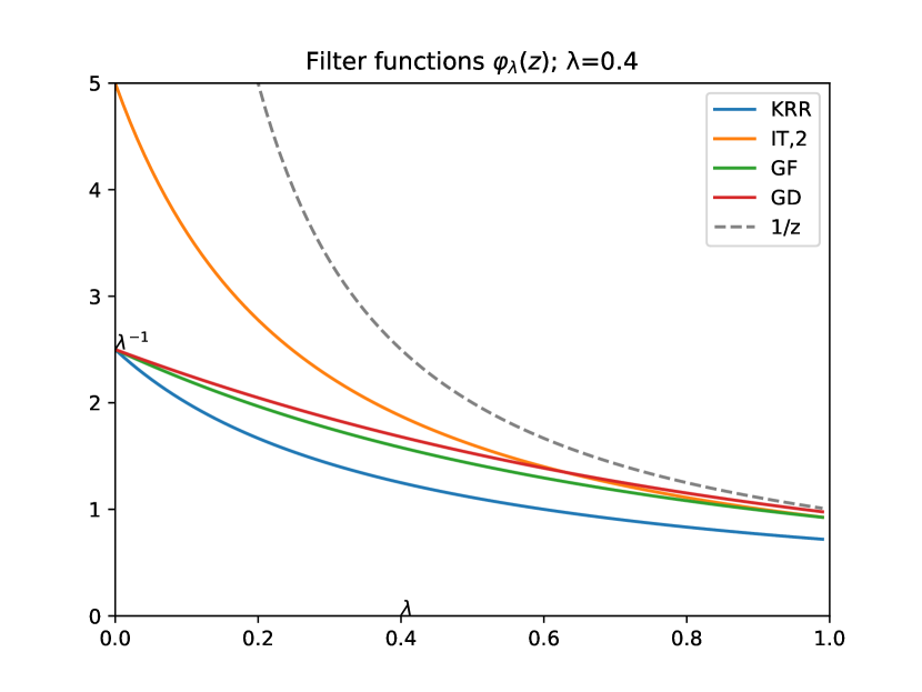
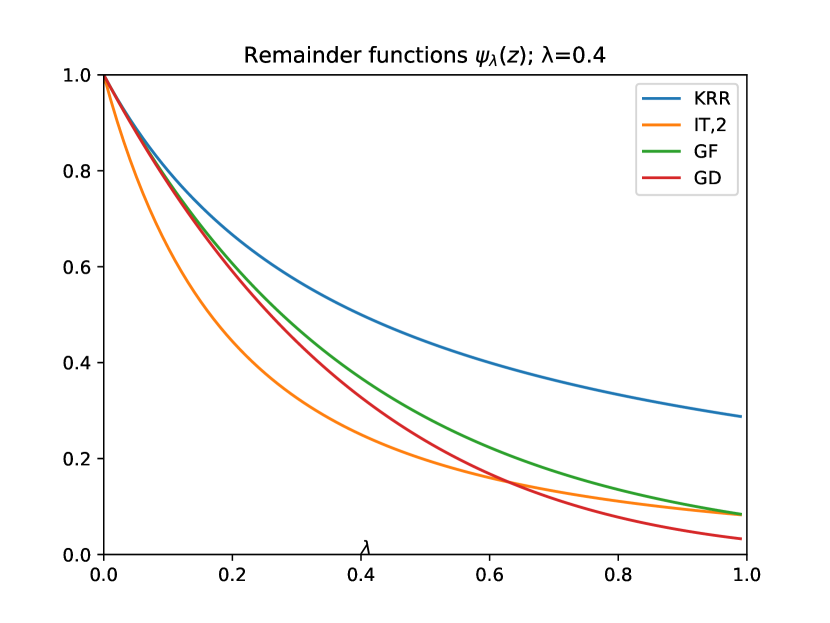
Figure 1: An illustration of the filter functions $\varphi_{\lambda}$ and $\psi_{\lambda}$.

Example 2.4 (Kernel ridge regression).

The filter function of kernel ridge regression (KRR) is well known to be

$$\varphi_{\lambda}^{\mathrm{KR}}(z)=\frac{1}{z+\lambda},\quad\psi_{\lambda}^{\mathrm{KR}}(z)=\frac{\lambda}{z+\lambda}.$$ (21)

Both $\varphi_{\lambda}$ and $\psi_{\lambda}$ are analytic on $\left\{z\in\mathbb{C}:\real z>-\lambda\right\}\supset D_{\lambda}$. This filter function is of qualification only $\tau_{\max}=1$.

Example 2.5 (Iterated ridge regression).

To overcome the limited qualification of KRR, Rosasco et al. (2005) introduce following iterated ridge (or iterated Tikhonov) method. Let $p\geq 1$ be fixed. We define

$$\varphi_{\lambda}^{\mathrm{IT,p}}(z)=\frac{1}{z}\left[1-\frac{\lambda^{p}}{(z+\lambda)^{p}}\right],\quad\psi^{\mathrm{IT,p}}_{\lambda}(z)=\frac{\lambda^{p}}{(z+\lambda)^{p}}.$$ (22)

It is easy to show that $z=0$ is a removable singular point of $\varphi_{\lambda}^{\mathrm{IT,p}}(z)$ and both $\varphi_{\lambda}^{\mathrm{IT,p}}(z)$ and $\psi_{\lambda}^{\mathrm{IT,p}}(z)$ are analytic on $\left\{z\in\mathbb{C}:\real z>-\lambda\right\}\supset D_{\lambda}$. The merit of this filter function is that it has qualification $\tau_{\max}=p$.

To understand the name “iterated”, let us consider the particular case $p\in\mathbb{N}^{*}$. Then,

$$\varphi^{\mathrm{IT,p}}_{\lambda}(z)=\sum_{r=1}^{p}\lambda^{r-1}(z+\lambda)^{-r},$$

and the method is obtained by iterating the ridge method $p$ times:

$$(T_{X}+\lambda)h_{i}=\hat{g}_{Z}+\lambda h_{i-1},\quad i=1,\dots,p.$$

Example 2.6 (Gradient flow).

The gradient flow method (Yao et al., 2007) is another popular regularization method. Let us consider the empirical loss

$$L(f)=\frac{1}{2n}\sum_{i=1}^{n}(f(x_{i})-y_{i})^{2}=\frac{1}{2n}\sum_{i=1}^{n}(K_{x_{i}}^{*}f-y_{i})^{2},\quad f\in\mathcal{H}.$$

Then, with the initial value $f_{0}=0$, $\dot{f}_{t}=-\nabla_{f}L(f_{t})$ defines a gradient flow in $\mathcal{H}$. The gradient flow equation, which can be solved in closed-form, gives the filter function

$$\varphi_{\lambda}^{\mathrm{GF}}(z)=\frac{1-e^{-tz}}{z},\quad\psi_{\lambda}^{\mathrm{GF}}(z)=e^{-tz},\quad t=\lambda^{-1}.$$ (23)

It is also easy to show that $z=0$ is a removable singular point of $\varphi_{\lambda}^{\mathrm{GF}}(z)$, so both $\varphi_{\lambda}^{\mathrm{GF}}(z)$ and $\psi_{\lambda}^{\mathrm{GF}}(z)$ are analytic on the whole complex plane. Moreover, elementary inequalities can show that the gradient flow method has qualification $\tau_{\max}=\infty$ with diverging $F_{\tau}=(\tau/e)^{\tau}$.

Example 2.7 (Gradient descent).

The gradient descent method is the discrete version of gradient flow. Let $\eta>0$ be a fixed step size. Then, iterating gradient descent with respect to the empirical loss $t$ steps yields the filter function

$$\begin{aligned} \varphi_{\lambda}^{\mathrm{GD}}(z)&=\eta\sum_{k=0}^{t-1}(1-\eta z)^{k}=\frac{1-(1-\eta z)^{t}}{z},\quad\lambda=(\eta t)^{-1},\\ \psi_{\lambda}^{\mathrm{GD}}(z)&=(1-\eta z)^{t}.\end{aligned}$$ (24)

Moreover, when $\eta$ is small enough, say $\eta<1/(2\kappa^{2})$, we have $\real(1-\eta z)>0$ for $z\in D_{\lambda}$, so we can take the single-valued branch of $(1-\eta z)^{t}$ even when $t$ is not an integer. Therefore, we can extend the definition of the filter function so that $\lambda$ can be arbitrary and $t=(\eta\lambda)^{-1}$. It is also easy to show that $z=0$ is a removable singular point of $\varphi_{\lambda}^{\mathrm{GD}}(z)$. Consequently, $\varphi_{\lambda}^{\mathrm{GD}}(z)$ and $\psi_{\lambda}^{\mathrm{GD}}(z)$ are analytic on $D_{\lambda}$. Similar to the gradient flow method, the gradient descent method is also of qualification $\tau_{\max}=\infty$ with $F_{\tau}=(\tau/e)^{\tau}$.

2.3 Notations

We denote by $\#A$ the cardinality of a set $A$. We use the big-O notations $O(\cdot),\Omega(\cdot),\Theta(\cdot)$, $o(\cdot)$. and also their probability versions $O_{\mathbb{P}}(\cdot)$, $\Omega_{\mathbb{P}}(\cdot)$, $\Theta_{\mathbb{P}}(\cdot)$ and $o_{\mathbb{P}}(\cdot)$. Let $(\xi_{n})_{n\geq 1}$ be a sequence of non-negative random variables and $(a_{n})_{n\geq 1}$ a sequence of positive numbers. We say $\xi_{n}=O_{\mathbb{P}}(a_{n})$ if for any $\delta>0$, there exists $N_{\delta}$ and $M_{\delta}$ such that when $n\geq N_{\delta}$, $\mathbb{P}\left\{\absolutevalue{\xi_{n}}\leq M_{\delta}a_{n}\right\}\geq 1-\delta$. The notation $\Omega_{\mathbb{P}}(a_{n})$ is defined similarly and $\xi_{n}=\Theta_{\mathbb{P}}(a_{n})$ iff $\xi_{n}=O_{\mathbb{P}}(a_{n})$ and $\xi_{n}=\Omega_{\mathbb{P}}(a_{n})$ both hold. Moreover, we say $\xi_{n}=o_{\mathbb{P}}(a_{n})$ if $\xi_{n}/a_{n}$ converges in probability to 0. Also, we sometimes write $a_{n}\asymp b_{n}$ if $a_{n}=\Theta(b_{n})$.

3 Main results

3.1 More assumptions

Before stating our main theorem, we introduce two assumptions. The first assumption concerns about the noise. This assumption is quite standard and is satisfied if the noise is independent of the input $x$ and has a bounded variance.

Assumption 4 (Noise).

We assume

$$\mathbb{E}_{(x,y)\sim\rho}\left[\left(y-f^{*}(x)\right)^{2}\;\Big{|}\;x\right]=\sigma^{2}>0,\quad\mu\text{-a.e. }x\in\mathcal{X},$$ (25)

The second assumption is about the regression function $f^{*}$. Recall the definition of interpolation spaces and that $\{e_{m,l}:~{}m\geq 1,~{}1\leq l\leq d_{m}\}$ consists of an orthogonal set in $L^{2}$. Then, we first assume that the regression function admits the following expansion in the sense of $L^{2}$-norm:

$$f^{*}=\sum_{m=1}^{\infty}\sum_{l=1}^{d_{m}}f_{m,l}e_{m,l}.$$ (26)

Here we note that $\bar{f}_{m}^{2}\coloneqq\sum_{l=1}^{d_{m}}\absolutevalue{f_{m,l}}^{2}=\norm{P_{V_{m}}f^{*}}_{L^{2}}^{2}$ is invariant of the choice of $\{e_{m,l}\}_{l=1}^{d_{m}}$ which is an orthogonal basis of $V_{m}$. Then, we assume that the regression function satisfies the following source condition.

Assumption 5 (Source).

There exists some $s>0$ such that $f^{*}\in[\mathcal{H}]^{t}$ for any $t<s$, $f^{*}\neq 0$, and if $s<2\tau_{\max}$,

$$\sum_{m:\mu_{m}<\lambda}\sum_{l=1}^{d_{m}}\absolutevalue{f_{m,l}}^{2}=\sum_{m:\mu_{m}<\lambda}\bar{f}_{m}^{2}=\Omega(\lambda^{s}).$$ (27)

This assumption assumes that the regression function can be approximately described by a power-law decay with smoothness index $s$, but it does not require that the coefficient of $f^{*}$ decays exactly in a power-law manner, which allows a wider range of regression functions to be considered. We note that since we have to establish the exact generalization error curve, the lower bound is also necessary, which is presented in a tail sum manner. The following shows some examples of regression functions satisfying Assumption 5.

Example 3.1 (Exact power-law $f^{*}$).

Let Assumption 1 hold and $\sum_{k=1}^{m}d_{k}\asymp m^{\gamma}$ for some $\gamma\geq 1$. Suppose $f^{*}$ satisfy that $\bar{f}_{m}\asymp m^{-(\gamma p+1)/2}$ for some $p>1$. Then $f^{*}$ satisfies Assumption 5 for $s=\frac{p}{\beta}$. In particular, with a little abuse of notation, if we rearrange $(f_{m,l})$ as

$$(f_{j})_{j\geq 1}=(f_{1,1},\dots,f_{1,d_{1}},f_{2,1},\dots,f_{m,1},\dots,f_{m,d_{m}},\dots).$$

Then, this example includes the case $\absolutevalue{f_{j}}\asymp\lambda_{j}^{\frac{s}{2}}j^{-\frac{1}{2}}\asymp j^{-\frac{s\beta+1}{2}}$ considered in Li et al. (2023); Cui et al. (2021).

We can also consider the following case that there are some gaps in the coefficients of $f^{*}$.

Example 3.2.

In this example, we assume Assumption 1 holds and consider the $(f_{j})_{j\geq 1}$ introduced in the previous example. Suppose that for some $q\geq 1,p>1$,

$$\begin{cases}\absolutevalue{f_{j(l)}}\asymp l^{-(p+1)/2},&l=1,2,\dots,\\ f_{j}=0,&\text{otherwise,}\end{cases}$$

where $j(l)\asymp l^{q}$. Then, $f^{*}$ satisfies Assumption 5 for $s=p/(q\beta)$.

3.2 Main theorem

Let us first introduce the two deterministic quantities that characterize the bias and the variance respectively. We define the main bias term by

$$\mathcal{R}_{\varphi}^{2}(\lambda;f^{*}) \coloneqq\norm{\psi_{\lambda}(T)f^{*}}_{L^{2}}^{2}=\sum_{m=1}^{\infty}\psi_{\lambda}(\mu_{m})^{2}\sum_{l=1}^{d_{m}}\absolutevalue{f_{m,l}}^{2}=\sum_{m=1}^{\infty}\psi_{\lambda}(\mu_{m})^{2}\bar{f}_{m}^{2}.$$ (28)

For the variance term, we extend the definition of effective dimension (Caponnetto and De Vito, 2007) to introduce the $\varphi$-effective dimension of order $p\geq 1$ by

$$\mathcal{N}_{p,\varphi}(\lambda)\coloneqq\sum_{j=1}^{\infty}\left[\lambda_{j}\varphi_{\lambda}(\lambda_{j})\right]^{p}=\sum_{m=1}^{\infty}d_{m}\left[\mu_{m}\varphi_{\lambda}(\mu_{m})\right]^{p}.$$ (29)

In particular, $\varphi^{\mathrm{KR}}$-effective dimension of order $p=1$ is just the ordinary effective dimension considered in the previous work (see (36) in the proof).

Theorem 3.1.

Under Assumptions 1,2,3,4 and 5, for any $\lambda=\lambda(n)\to 0$, we have

• If $\lambda=\Omega(n^{-\theta})$ for some $\theta<\beta$, then

  $$\mathbb{E}\left[\norm{\hat{f}_{\lambda}-f^{*}}_{L^{2}}^{2}~{}\Big{|}~{}X\right]=(1+o_{\mathbb{P}}(1))\left(\mathcal{R}_{\varphi}^{2}(\lambda;f^{*})+\frac{\sigma^{2}}{n}\mathcal{N}_{2,\varphi}(\lambda)\right),$$ (30)

  where $\mathcal{R}_{\varphi}^{2}(\lambda;f^{*})$ and $\mathcal{N}_{2,\varphi}(\lambda)$ are two deterministic quantities defined in (28) and (29) respectively.

• If $\lambda=O(n^{-\beta})$, then for any $\varepsilon>0$,

  $$\mathbb{E}\left[\norm{\hat{f}_{\lambda}-f^{*}}_{L^{2}}^{2}~{}\Big{|}~{}X\right]=\Omega_{\mathbb{P}}\left((\ln n)^{-\varepsilon}\sigma^{2}\right),$$ (31)

  where we notice that the hidden constant in $\Omega_{\mathbb{P}}(\cdot)$ depends on $\varepsilon$.

3.3 Discussion

In this subsection, we discuss our main result in the following aspect:

Minimax optimal rate

Theorem 3.1 naturally recovers the minimax optimal rates of spectral algorithms that have been derived in previous works  (see Lin et al. (2018); Zhang et al. (2023) and also the references therein). Let us suppose further that $f^{*}\in[\mathcal{H}]^{s}$ as in the standard literature and $s\leq 2\tau$. Then, for the bias term, Lemma 4.4 shows that

$$\mathcal{R}_{\varphi}^{2}(\lambda;f^{*})=\norm{\psi_{\lambda}(T)f^{*}}_{L^{2}}^{2}=O(\lambda^{s}).$$

For the variance term, Lemma LABEL:lem:EffectiveDimEstimation and the remark after it show that

$$\frac{\sigma^{2}}{n}\mathcal{N}_{2,\varphi}(\lambda)\asymp\frac{\sigma^{2}}{n}\lambda^{-1/\beta}.$$

Consequently, choosing $\lambda\asymp n^{-\theta}$ with $\theta=\frac{1}{s\beta+1}$ (as in the previous literature) yields the optimal rate

$$\mathbb{E}\left[\norm{\hat{f}_{\lambda}-f^{*}}_{L^{2}}^{2}~{}\Big{|}~{}X\right]=O_{\mathbb{P}}\left(n^{-\frac{s\beta}{s\beta+1}}\right).$$

Exact generalization error curve

Our result provides a complete picture of the generalization error of spectral algorithms, showing the effect of the choice of the regularization parameter, the source condition of the regression function, the noise level and also the choice of the filter function. In terms of regularization, as the regularization strength $\lambda$ decreases, the bias decreases while the variance increases, showing that the bias-variance trade-off also exists for spectral algorithms and the learning curve is U-shaped as our traditional belief. It also suggests that a proper choice of $\lambda$ is necessary to achieve the optimal rate.

A strength of our result is that it provides the exact $1+o_{\mathbb{P}}(1)$ form of the generalization error for a specific spectral algorithm when $\lambda$ lies in the reasonable range. In comparison, the previous works (for example, Caponnetto and De Vito (2007); Lin et al. (2018); Zhang et al. (2023)) on minimax optimal rate only considered the upper bound and focused on the best choice of $\lambda$ and the best rate of convergence, while our result gives the exact generalization error curve with matching upper and lower bound for any choice of $\lambda$. The recent work (Li et al., 2023) proved rigorously the learning curves of KRR, but only asymptotic rates (in the form of $\Theta_{\mathbb{P}}(n^{-r})$) are provided, so our result is also a refinement of their result even in the KRR case. For general spectral algorithms, as far as we know, we are the first to provide such exact generalization error curves.

The implication of the $1+o_{\mathbb{P}}(1)$ form of exact generalization error is that it allows us to consider the constant factor in the generalization error. It could reflect precisely how the magnitude of the regression function and the noise affect the generalization error. Moreover, from the oracle viewpoint, minimizing the sum of the two terms in (30) would result in the best choice of $\lambda=\lambda(n)$ and the best generalization error, going beyond merely the asymptotic rate.

Interpolating regime

We refer to the case of weak regularization, namely $\lambda=\lambda(n)=O(n^{-\beta})$, as the interpolating regime. Theorem 3.1 shows that in this regime, the generalization error is of order $\Omega_{\mathbb{P}}((\ln n)^{-\varepsilon})$, which is nearly a constant, so estimator does not generalize at all.

The performance of kernel methods in the interpolating regime is also considered in the previous literature. Under restricted settings, several works  (Rakhlin and Zhai, 2018; Buchholz, 2022; Beaglehole et al., 2022) shown the inconsistency of the kernel minimum-norm interpolator, which is the $\lambda\to 0^{+}$ limit of spectral algorithms. Being the most relevant with this paper, Li et al. (2023) showed that for general RKHSs associated with a Hölder continuous kernel satisfying the embedding index condition, the generalization error of KRR in the interpolating regime is $\Omega_{\mathbb{P}}(n^{-\varepsilon})$ for any $\varepsilon>0$. In comparison, we remove the condition of Hölder continuity and also provide an improved lower bound $\Omega_{\mathbb{P}}((\ln n)^{-\varepsilon})$ for spectral algorithms in the interpolating regime by refine the analysis using the condition of regular RKHS. We believe that this improved lower bound further confirms kernel methods do not generalize in the interpolating regime, highlighting the necessity of the regularization.

Saturation effect of higher order

The saturation effect refers to the phenomenon that, for a certain spectral algorithm with limited qualification, it cannot achieve the minimax optimal rate of convergence when the smoothness of the regression function exceeds its qualification. Since the traditional literature only provides the upper bound of the generalization error, they cannot prove the saturation effect. The recent work Li et al. (2023) rigorously proved the saturation effect for KRR, whose qualification is $\tau_{\max}=1$, but there is still result for other spectral algorithms with higher (but limited) qualification, such as the iterated ridge regularization (see Example 2.5).

Thanks to the exact generalization error curve, we can prove the saturation effect for spectral algorithms with higher qualification. Let us consider a spectral algorithm such that it has limited qualification $\tau_{\max}<\infty$, which is the case of the iterated ridge regularization. Then, for $f^{*}\in[\mathcal{H}]^{s}$ with $s\geq 2\tau_{\max}$ and $f^{*}\neq 0$ it is easy to see that

$$\mathcal{R}_{\varphi}^{2}(\lambda;f^{*})=\sum_{m=1}^{\infty}\psi_{\lambda}(\mu_{m})^{2}\bar{f}_{m}^{2}\geq\sum_{m=1}^{\infty}\underline{F}\lambda^{2\tau}\bar{f}_{m}^{2}=\underline{F}\norm{f^{*}}_{L^{2}}^{2}\lambda^{2\tau}.$$

Consequently, with the upper bound in Lemma 4.4, we conclude that $\mathcal{R}_{\varphi}^{2}(\lambda;f^{*})\asymp\lambda^{2\tau}$. Then, when $\lambda$ is not too small, the main theorem gives

$$\mathbb{E}\left[\norm{\hat{f}_{\lambda}-f^{*}}_{L^{2}}^{2}~{}\Big{|}~{}X\right] =(1+o_{\mathbb{P}}(1))\left(\mathcal{R}_{\varphi}^{2}(\lambda;f^{*})+\frac{\sigma^{2}}{n}\mathcal{N}_{2,\varphi}(\lambda)\right)$$

$$=\Omega_{\mathbb{P}}\left(\lambda^{2\tau}+\frac{\sigma^{2}}{n}\lambda^{-1/\beta}\right)=\Omega_{\mathbb{P}}\left(n^{-\frac{2\tau\beta}{2\tau\beta+1}}\right).$$

To cover the case when $\lambda$ can possibly be too small, we can consider $\bar{\lambda}=\max(\lambda,n^{-\theta})$ for some $\theta<\beta$ and apply the monotonicity of the variance term (Lemma 4.14) as in Li et al. (2023). We formulate it as a corollary.

Corollary 3.2 (Saturation effect).

Suppose Assumptions 1,2,3,4 hold. Let $\varphi_{\lambda}$ be a filter function with qualification $\tau=\tau_{\max}<\infty$. Then, for any non-zero $f^{*}\in[\mathcal{H}]^{s}$ for $s\geq 2\tau$, for any choice of $\lambda=\lambda(n)\to 0$, we have

$$\mathbb{E}\left[\norm{\hat{f}_{\lambda}-f^{*}}_{L^{2}}^{2}~{}\Big{|}~{}X\right]=\Omega_{\mathbb{P}}\left(n^{-\frac{2\tau\beta}{2\tau\beta+1}}\right).$$ (32)

Moreover, the lower bound is attained when $\lambda\asymp n^{-\theta}$ for $\theta=\frac{\beta}{2\tau\beta+1}$.

The analytic functional argument

As one of our main contributions, we develop a new analytic functional argument based on analytic functional calculus to analyze the generalization error of spectral algorithms. First, we would like to illustrate the difficulties here and why the existing techniques are not applicable. The traditional literature on the optimal rate focused only on the upper bound and their approaches, which are based on the approximation-estimation decomposition  (for example, Eq. (88) in Zhang et al. (2023)), are not applicable for the lower bound. Moreover, it is in general more difficult to provide the lower bound than the upper bound since the former requires the error term to be infinitesimal, For the simple case of KRR, the rigorous work (Li et al., 2023) determined the asymptotic rate of convergence, but the proof method must rely on the resolvent identity of KRR, that is,

$$\varphi_{\lambda}^{\mathrm{KR}}(A)-\varphi_{\lambda}^{\mathrm{KR}}(B)=(A+\lambda)^{-1}-(B+\lambda)^{-1}=(A+\lambda)^{-1}(B-A)(B+\lambda)^{-1},$$

and also $\psi_{\lambda}^{\mathrm{KR}}(A)=\lambda(A+\lambda)^{-1}$. This identity is crucial for concentrating the random terms (see (35)) to the non-random counterpart appearing on the right hand side of (30), where we will encounter quantities like $\varphi_{\lambda}(T)-\varphi_{\lambda}(T_{X})$ and $\psi_{\lambda}(T)-\psi_{\lambda}(T_{X})$. However, for general spectral algorithms, it is impossible to derive similar identity. Moreover, the effect of $\lambda$ must also be taken into consideration.

Our “analytic functional argument” overcomes these difficulties by the following novel idea. For analytic spectral algorithm, analytic functional calculus gives that

$$\varphi_{\lambda}(A)-\varphi_{\lambda}(B) =-\frac{1}{2\pi i}\oint_{\Gamma}\varphi_{\lambda}(z)\left[R_{A}(z)-R_{B}(z)\right]\differential z$$

$$=\frac{1}{2\pi i}\oint_{\Gamma}R_{B}(z)(A-B)R_{A}(z)\varphi_{\lambda}(z)\differential z,$$

where $R_{A}(z)=(A-z)^{-1}$ is the resolvent of $A$ and $\Gamma$ is a contour. Then, the terms in the integral resemble that of KRR (but note that now $z$ a complex number now). Surprisingly, with carefully chosen contour $\Gamma$ depending on $\lambda$, this crucial formula allows us to apply the concentration results obtained for the resolvent and derive very sharp estimations, leading to the exact generalization error curve. We believe that this novel technique is of independent interest and can be applied to other problems.

4 Proof

4.1 Proof sketch

The proof idea is quite direct. The first step is the traditional bias-variance decomposition, which is also standard in the literature (Li et al., 2023). Let us first define some quantities derived from conditional expectation on the sample points $X$:

$$\tilde{g}_{X} \coloneqq\mathbb{E}\left(g_{Z}\big{|}X\right)=\frac{1}{n}\sum_{i=1}^{n}K_{x_{i}}f^{*}(x_{i})\in\mathcal{H},$$ (33)

$$\tilde{f}_{\lambda} \coloneqq\mathbb{E}\left(\hat{f}_{\lambda}\big{|}X\right)=\varphi_{\lambda}(T_{X})\tilde{g}_{X}\in\mathcal{H}.$$ (34)

Proposition 4.1.

Under Assumption 4, we have

$$\begin{aligned} \mathbb{E}\left[\norm{\hat{f}_{\lambda}-f^{*}}^{2}_{L^{2}}\;\Big{|}\;X\right]&=\norm{\tilde{f}_{\lambda}-f^{*}}^{2}_{L^{2}}+\frac{\sigma^{2}}{n^{2}}\sum_{i=1}^{n}\norm{\varphi_{\lambda}(T_{X})k(x_{i},\cdot)}^{2}_{L^{2}}\\ &\eqqcolon\mathbf{Bias}^{2}(\lambda)+\mathbf{Var}(\lambda),\end{aligned}$$ (35)

where we note that both $\mathbf{Bias}^{2}(\lambda)$ and $\mathbf{Var}(\lambda)$ are still random variables depending on $X$.

Then, we will show respectively in Theorem 4.13 and Theorem 4.18 that for $\lambda=\Omega(n^{-\theta})$, $\theta<\beta$,

$$\mathbf{Var}(\lambda) =(1+o_{\mathbb{P}}(1))\frac{\sigma^{2}}{n}\mathcal{N}_{2,\varphi}(\lambda),$$

$$\mathbf{Bias}^{2}(\lambda) =\mathcal{R}_{\varphi}^{2}(\lambda;f^{*})+o_{\mathbb{P}}(1)\left(\mathcal{R}_{\varphi}^{2}(\lambda;f^{*})+\frac{1}{n}\mathcal{N}_{2,\varphi}(\lambda)\right).$$

Moreover, in Corollary 4.15, using the monotonicity of $\mathbf{Var}(\lambda)$, we can also provide a lower bound of $\mathbf{Var}(\lambda)$ when $\lambda=O(n^{-\beta})$. Then, pulling all together finishes the proof of the Theorem 3.1.

Organization

In the following, we first give a simple proof of the bias-variance decomposition in Proposition 4.1. In Subsection 4.2, we will derive estimations of some fundamental quantities that will be used later. In Subsection 4.3, we will use concentration inequalities to obtain high-probability bounds on some intermediate but crucial quantities. In Subsection 4.4, we recall some basic facts about analytic functional calculus and define the contour that is essential in our the proof. Finally, we prove the estimation of the two terms in Subsection 4.5 and Subsection 4.6.

More notations

In the proof, we will denote by $C,c$ generic positive constants that may change from line to line. We use $\norm{\cdot}_{\mathscr{B}(H)}$ or simply $\norm{\cdot}$ to represent the operator norm on a Hilbert space $H$. We also denote by $x^{+}=\max(x,0)$.

Proof of Proposition 4.1.

Let $\epsilon_{i}=y_{i}-f^{*}(x_{i})$ be the noise. Then, plugging (15) into (19), we get

$$\hat{f}_{\lambda} =\varphi_{\lambda}(T_{X})\hat{g}_{Z}=\varphi_{\lambda}(T_{X})\left(\frac{1}{n}\sum_{i=1}^{n}K_{x_{i}}(f^{*}(x_{i})+\epsilon_{i})\right)$$

$$=\varphi_{\lambda}(T_{X})\frac{1}{n}\sum_{i=1}^{n}K_{x_{i}}f^{*}(x_{i})+\frac{1}{n}\sum_{i=1}^{n}\epsilon_{i}\varphi_{\lambda}(T_{X})k_{x_{i}}$$

$$=\tilde{f}_{\lambda}+\frac{1}{n}\sum_{i=1}^{n}\epsilon_{i}\varphi_{\lambda}(T_{X})k_{x_{i}},$$

so

$$\hat{f}_{\lambda}-f^{*}=\tilde{f}_{\lambda}-f^{*}+\frac{1}{n}\sum_{i=1}^{n}\epsilon_{i}\varphi_{\lambda}(T_{X})k_{x_{i}}.$$

Taking conditional expectation on $X$ and using the fact that $\{\epsilon_{i}\}_{i=1}^{n}$ are i.i.d. mean-zero random variables conditioned on $X$ and also Assumption 4, we get

$$\mathbb{E}\left[\norm{\hat{f}_{\lambda}-f^{*}}^{2}_{L^{2}}\;\Big{|}\;X\right] =\mathbb{E}\left[\left\langle{\hat{f}_{\lambda}-f^{*},~{}\hat{f}_{\lambda}-f^{*}}\right\rangle_{L^{2}}\;\Big{|}\;X\right]$$

$$=\norm{\tilde{f}_{\lambda}-f^{*}}^{2}_{L^{2}}+2\mathbb{E}\left[\real\left\langle{\tilde{f}_{\lambda}-f^{*},~{}\frac{1}{n}\sum_{i=1}^{n}\epsilon_{i}\varphi_{\lambda}(T_{X})k_{x_{i}}}\right\rangle_{L^{2}}\;\Big{|}\;X\right]$$

$$\quad+\mathbb{E}\left[\norm{\frac{1}{n}\sum_{i=1}^{n}\epsilon_{i}\varphi_{\lambda}(T_{X})k_{x_{i}}}^{2}_{L^{2}}\;\Big{|}\;X\right]$$

$$=\norm{\tilde{f}_{\lambda}-f^{*}}^{2}_{L^{2}}+\frac{1}{n^{2}}\mathbb{E}\left[\left\langle{\sum_{i=1}^{n}\epsilon_{i}\varphi_{\lambda}(T_{X})k_{x_{i}},~{}\sum_{i=1}^{n}\epsilon_{i}\varphi_{\lambda}(T_{X})k_{x_{i}}}\right\rangle_{L^{2}}\;\Big{|}\;X\right]$$

$$=\norm{\tilde{f}_{\lambda}-f^{*}}^{2}_{L^{2}}+\frac{1}{n^{2}}\sum_{i=1}^{n}\mathbb{E}(\epsilon_{i}^{2}|X)\norm{\varphi_{\lambda}(T_{X})k(x_{i},\cdot)}^{2}_{L^{2}}$$

$$=\norm{\tilde{f}_{\lambda}-f^{*}}^{2}_{L^{2}}+\frac{\sigma^{2}}{n^{2}}\sum_{i=1}^{n}\norm{\varphi_{\lambda}(T_{X})k(x_{i},\cdot)}^{2}_{L^{2}}.$$

∎

4.2 Fundamental controls

Denote the effective dimension (of power $p\geq 1$) of the RKHS $\mathcal{H}$ by

$$\mathcal{N}_{p}(\lambda)\coloneqq\sum_{i=1}^{\infty}\left(\frac{\lambda_{i}}{\lambda+\lambda_{i}}\right)^{p}.$$ (36)

This quantity corresponds to the $\varphi^{\mathrm{KR}}$-effective dimension defined previously in (29). When $p=1$, it is the ordinary effective dimension in the literature (Caponnetto and De Vito, 2007).

Let us provide first the controls of the regularized basis functions using the regular RKHS condition.

Lemma 4.2.

Under Assumption 2, for any $x\in\mathcal{X}$,

$$\norm{\varphi_{\lambda}^{1/2}(T)k_{x}}_{\mathcal{H}}^{2} \leq M\mathcal{N}_{1,\varphi}(\lambda),\qquad\norm{\varphi_{\lambda}(T)k_{x}}_{L^{2}}^{2}\leq M\mathcal{N}_{2,\varphi}(\lambda).$$ (37)

In particular, for $\varphi_{\lambda}=\varphi_{\lambda}^{\mathrm{KR}}$,

$$\norm{T_{\lambda}^{-1/2}k_{x}}_{\mathcal{H}}^{2} \leq M\mathcal{N}_{1}(\lambda),\qquad\norm{T_{\lambda}^{-1}k_{x}}_{L^{2}}^{2}\leq M\mathcal{N}_{2}(\lambda).$$ (38)

Proof.

Using the spectral decomposition (3) and also Mercer’s decomposition (4), we have

$$\norm{\varphi_{\lambda}^{1/2}(T)k_{x}}_{\mathcal{H}}^{2} =\norm{\varphi_{\lambda}^{1/2}(T)\sum_{m=1}^{\infty}\mu_{m}\sum_{l=1}^{d_{m}}\overline{e_{m,l}(x)}e_{m,l}}_{\mathcal{H}}^{2}$$

$$=\norm{\sum_{m=1}^{\infty}\varphi_{\lambda}^{1/2}(\mu_{m})\mu_{m}\sum_{l=1}^{d_{m}}\overline{e_{m,l}(x)}e_{m,l}}_{\mathcal{H}}^{2}$$

$$=\sum_{m=1}^{\infty}\mu_{m}\varphi_{\lambda}(\mu_{m})\sum_{l=1}^{d_{m}}\absolutevalue{e_{m,l}(x)}^{2}.$$

Then, noticing that $a_{m}=\mu_{m}\varphi_{\lambda}(\mu_{m})$ is decreasing since $\mu_{m}$ is decreasing and $t\varphi_{\lambda}(t)$ decreases as $t$ decreases, Proposition A.3 and Assumption 2 yield

$$\norm{\varphi_{\lambda}^{1/2}(T)k_{x}}_{\mathcal{H}}^{2}\leq M\sum_{m=1}^{\infty}\mu_{m}\varphi_{\lambda}(\mu_{m})d_{m}=M\mathcal{N}_{1,\varphi}(\lambda).$$

Similarly,

$$\norm{\varphi_{\lambda}(T)k_{x}}_{L^{2}}^{2}=\sum_{m=1}^{\infty}\left(\mu_{m}\varphi_{\lambda}(\mu_{m})\right)^{2}\sum_{l=1}^{d_{m}}\absolutevalue{e_{m,l}(x)}^{2}\leq M\mathcal{N}_{2}(\lambda).$$

∎

Under the power-law decay Assumption 1, we have the following asymptotics of the effective dimension  (see, for example, Li et al. (2023, Proposition B.3)).

Lemma 4.3.

Let Assumption 1 hold and $\varphi_{\lambda}$ be a filter function satisfying (17) and (18). Then, for any $p\geq 1$ and $\lambda>0$, we have

$$\mathcal{N}_{p,\varphi}(\lambda)\asymp\lambda^{-1/\beta}.$$ (39)

The following lemma controls the residual term, which will be used in the proof of the bias term.

Lemma 4.4.

Suppose $f^{*}\in[\mathcal{H}]^{t}$. Let $\varphi_{\lambda}$ be a filter function of qualification $\tau$ and $f^{*}_{\lambda}=\varphi_{\lambda}(T)Tf^{*}$. Then, for $\gamma\in[0,t]$,

$$\norm{f^{*}-f^{*}_{\lambda}}_{[\mathcal{H}]^{\gamma}}=\norm{\psi_{\lambda}(T)f^{*}}_{[\mathcal{H}]^{\gamma}}\leq F_{\theta}\kappa^{(t-\gamma-2\tau)^{+}}\norm{f^{*}}_{[\mathcal{H}]^{t}}\lambda^{\theta},$$ (40)

where $\theta=\min\left(\frac{t-\gamma}{2},\tau\right)$. In addition, for $\gamma\in[0,2+t]$,

$$\norm{f^{*}_{\lambda}}_{[\mathcal{H}]^{\gamma}}\leq E\kappa^{(t-\gamma)^{+}}\norm{f^{*}}_{[\mathcal{H}]^{t}}\lambda^{-\frac{(\gamma-t)^{+}}{2}}.$$ (41)

Proof.

Since $f^{*}\in[\mathcal{H}]^{t}$, we can find $h\in L^{2}$ such that $f^{*}=T^{t/2}h$ and $\norm{h}_{L^{2}}=\norm{f^{*}}_{[\mathcal{H}]^{t}}$. Then,

$$\norm{\psi_{\lambda}(T)f^{*}}_{[\mathcal{H}]^{\gamma}} =\norm{T^{-\gamma/2}\psi_{\lambda}(T)T^{t/2}h}_{L^{2}}\leq\norm{T^{\frac{t-\gamma}{2}}\psi_{\lambda}(T)}_{\mathscr{B}(L^{2})}\norm{h}_{L^{2}}$$

$$\leq\norm{T^{\frac{(t-\gamma-2\tau)^{+}}{2})}}\norm{T^{\min(\frac{t-\gamma}{2},\tau)}\psi_{\lambda}(T)}_{\mathscr{B}(L^{2})}\norm{f^{*}}_{[\mathcal{H}]^{t}}$$

$$\leq F_{\theta}\kappa^{(t-\gamma-2\tau)^{+}}\norm{f^{*}}_{[\mathcal{H}]^{t}}\lambda^{\min(\frac{t-\gamma}{2},\tau)},$$

where $\theta=\min\left(\frac{t-\gamma}{2},\tau\right)$. For the second inequality, we have

$$\norm{f^{*}_{\lambda}}_{[\mathcal{H}]^{\gamma}} =\norm{T^{-\frac{\gamma}{2}}T\varphi_{\lambda}(T)T^{\frac{t}{2}}h}_{L^{2}}$$

$$\leq\norm{T^{\frac{2+t-\gamma}{2}}\varphi_{\lambda}(T)}_{\mathscr{B}(L^{2})}\norm{h}_{L^{2}}$$

$$\leq\norm{T^{\frac{(t-\gamma)^{+}}{2}}}\norm{T^{1-\frac{(\gamma-t)^{+}}{2}}\varphi_{\lambda}(T)}_{\mathscr{B}(L^{2})}\norm{h}_{L^{2}}$$

$$\leq E\kappa^{(t-\gamma)^{+}}\norm{f^{*}}_{[\mathcal{H}]^{t}}\lambda^{-\frac{(\gamma-t)^{+}}{2}},$$

where we use (78) for the second term in the last inequality. ∎

Proposition 4.5.

Let $f^{*}\in[\mathcal{H}]^{0}$. Suppose $\varphi_{\lambda}$ is a filter function defined in Definition 2.3 with qualification $\tau_{\max}$. Then,

$$R_{\varphi}^{2}(\lambda;f^{*})\geq\frac{1}{4}\sum_{m:\mu_{m}<\frac{\lambda}{2E}}\bar{f}_{m}^{2}$$

Moreover, if $\tau_{\max}<\infty$, we also have $R_{\varphi}^{2}(\lambda;f^{*})\geq\norm{f}_{L^{2}}^{2}\underline{F}\lambda^{2\tau_{\max}}$.

Consequently, under Assumption 5, we have

$$R_{\varphi}^{2}(\lambda;f^{*})=\Omega(\lambda^{\min(s,2\tau_{\max})}).$$ (42)

Proof.

Recall the definition of $R_{\varphi}^{2}(\lambda;f^{*})$ in (28). For the first estimation, using the last control in Lemma A.5, when $\mu_{m}\leq\frac{\lambda}{2E}$, we have $\psi_{\lambda}(\mu_{m})\geq 1/2$, so

$$R_{\varphi}^{2}(\lambda;f^{*})=\sum_{m=1}^{\infty}\psi_{\lambda}(\mu_{m})^{2}\bar{f}_{m}^{2}\geq\sum_{m:\mu_{m}<\frac{\lambda}{2E}}\psi_{\lambda}(\mu_{m})^{2}\bar{f}_{m}^{2}\geq\frac{1}{4}\sum_{m:\mu_{m}<\frac{\lambda}{2E}}\bar{f}_{m}^{2}.$$

For the second one, using the property (iv) in Definition 2.3, we have

$$R_{\varphi}^{2}(\lambda;f^{*})=\sum_{m=1}^{\infty}\psi_{\lambda}(\mu_{m})^{2}\bar{f}_{m}^{2}\geq\sum_{m=1}^{\infty}\underline{F}\lambda^{2\tau_{\max}}\bar{f}_{m}^{2}=\underline{F}\lambda^{2\tau_{\max}}\norm{f}_{L^{2}}^{2}.$$

∎

4.3 Concentrations

Using the regular RKHS condition, the following inequality is a refinement of the concentration in the previous literature (Li et al., 2023, Proposition 5.8). The main improvement is that the quantity $\mathcal{N}_{1}(\lambda)\asymp\lambda^{-1/\beta}$ appearing in the right-hand side is strictly smaller than the quantity $M_{\alpha}\lambda^{-\alpha}$, $\alpha>1/\beta$ appearing in their bound, which diverges as $\alpha\to 1/\beta$.

Proposition 4.6.

Under Assumption 2, for all $\delta\in(0,1)$, with probability at least $1-\delta$,

$$\norm{T_{\lambda}^{-\frac{1}{2}}(T-T_{X})T_{\lambda}^{-\frac{1}{2}}}_{\mathscr{B}(\mathcal{H})}\leq\frac{2}{3}u+\sqrt{u},$$ (43)

where

$$u=u(n,\lambda)=\frac{2M\mathcal{N}_{1}(\lambda)}{n}\ln{\frac{4(\norm{T}+\lambda)\mathcal{N}_{1}(\lambda)}{\delta\norm{T}}}.$$ (44)

Proof.

We will prove by Lemma A.8. Let us define

$$A(x)=T_{\lambda}^{-\frac{1}{2}}(T_{x}-T)T_{\lambda}^{-\frac{1}{2}}$$

and $A_{i}=A(x_{i})$. Then, it is easy to see that $\mathbb{E}(A_{i})=0$ and

$$\frac{1}{n}\sum_{i=1}^{n}A_{i}=T_{\lambda}^{-\frac{1}{2}}(T_{X}-T)T_{\lambda}^{-\frac{1}{2}},$$

which is the quantity of interest. Moreover, since

$$T_{\lambda}^{-\frac{1}{2}}T_{x}T_{\lambda}^{-\frac{1}{2}}=T_{\lambda}^{-\frac{1}{2}}K_{x}K_{x}^{*}T_{\lambda}^{-\frac{1}{2}}=T_{\lambda}^{-\frac{1}{2}}K_{x}\left[T_{\lambda}^{-\frac{1}{2}}K_{x}\right]^{*},$$

from (38) we have

$$\norm{T_{\lambda}^{-\frac{1}{2}}T_{x}T_{\lambda}^{-\frac{1}{2}}}_{\mathscr{B}(\mathcal{H})}=\norm{T_{\lambda}^{-\frac{1}{2}}K_{x}}_{\mathscr{B}(\mathbb{R},\mathcal{H})}^{2}=\norm{T_{\lambda}^{-\frac{1}{2}}k_{x}}_{\mathcal{H}}^{2}\leq M\mathcal{N}_{1}(\lambda).$$ (45)

By taking expectation, we also have $\norm{T_{\lambda}^{-\frac{1}{2}}TT_{\lambda}^{-\frac{1}{2}}}_{\mathscr{B}(\mathcal{H})}\leq M\mathcal{N}_{1}(\lambda)$. Therefore, we get

$$\norm{A}_{\mathscr{B}(\mathcal{H})}\leq\norm{T_{\lambda}^{-\frac{1}{2}}TT_{\lambda}^{-\frac{1}{2}}}_{\mathscr{B}(\mathcal{H})}+\norm{T_{\lambda}^{-\frac{1}{2}}T_{x}T_{\lambda}^{-\frac{1}{2}}}_{\mathscr{B}(\mathcal{H})}\leq 2M\mathcal{N}_{1}(\lambda)\eqqcolon L.$$

For the second part of the condition, using the fact that $\mathbb{E}(B-\mathbb{E}(B))^{2}\preceq\mathbb{E}(B^{2})$ and also $B^{2}\preceq\norm{B}B$ for a positive self-adjoint operator $B$, where $\preceq$ denotes the partial order induced by positive operators, we have

$$\mathbb{E}(A^{2})\preceq\mathbb{E}\left(T_{\lambda}^{-\frac{1}{2}}T_{x}T_{\lambda}^{-\frac{1}{2}}\right)^{2}\preceq L\mathbb{E}\left(T_{\lambda}^{-\frac{1}{2}}T_{x}T_{\lambda}^{-\frac{1}{2}}\right)=LTT_{\lambda}^{-1}\eqqcolon V,$$

where the second $\preceq$ comes from (45). Therefore,

$$\norm{V} =L\norm{TT_{\lambda}^{-1}}=L\frac{\lambda_{1}}{\lambda+\lambda_{1}},\qquad\Tr V=L\Tr\left[TT_{\lambda}^{-1}\right]=L\mathcal{N}_{1}(\lambda),$$

$$B =\ln\frac{4\tr V}{\delta\norm{V}}=\ln\frac{4(\lambda_{1}+\lambda)\mathcal{N}_{1}(\lambda)}{\delta\lambda_{1}}.$$

Finally, we note that the quantities in the lemma are:

$$\frac{2LB}{3n}=\frac{4M\mathcal{N}_{1}(\lambda)B}{3n}=\frac{2}{3}u,\qquad\frac{2\norm{V}B}{n}\leq\frac{2M\mathcal{N}_{1}(\lambda)B}{n}=u.$$

∎

The next lemma is a consequence of Proposition 4.6.

Lemma 4.7.

Suppose Assumption 2 holds. Fix $\delta\in(0,1)$. Let us denote

$$v=v(n,\lambda)=\frac{M\mathcal{N}_{1}(\lambda)}{n}\ln\frac{\mathcal{N}_{1}(\lambda)}{\delta}.$$ (46)

Suppose $\lambda=\lambda(n)\to 0$ satisfies $v(n,\lambda)=o(1)$. Then, when $n$ is sufficiently large, with probability at least $1-\delta$ we have

$$\norm{T_{\lambda}^{-1/2}(T-T_{X})T_{\lambda}^{-1/2}}\leq C\sqrt{v},$$ (47)

$$\begin{aligned} &\norm{T_{X\lambda}^{-1/2}T_{\lambda}^{1/2}}^{2}=\norm{T_{\lambda}^{1/2}T_{X\lambda}^{-1/2}}^{2}=\norm{T_{\lambda}^{1/2}T_{X\lambda}^{-1}T_{\lambda}^{1/2}}\leq 3,\\ &\norm{T_{\lambda}^{-1/2}T_{X\lambda}^{1/2}}^{2}=\norm{T_{X\lambda}^{1/2}T_{\lambda}^{-1/2}}^{2}=\norm{T_{\lambda}^{-1/2}T_{X\lambda}^{1}T_{\lambda}^{-1/2}}\leq 2,\end{aligned}$$ (48)

where $C$ is an absolute constant.

Proof.

(47) is a direct corollary of Proposition 4.6 with $v=o(1)$ and

$$u=\frac{2M\mathcal{N}_{1}(\lambda)}{n}\ln{\frac{4(\lambda_{1}+\lambda)\mathcal{N}_{1}(\lambda)}{\delta\lambda_{1}}}\leq C_{0}v$$

for some absolute constant $C_{0}$. For the second part, when $n$ is sufficiently large that $u\leq 1/4$,

$$\norm{T_{\lambda}^{-1/2}(T-T_{X})T_{\lambda}^{-1/2}}\leq\frac{2}{3}u+\sqrt{u}\leq\frac{2}{3}.$$

Noticing that $\left(T_{X\lambda}^{-1/2}T_{\lambda}^{1/2}\right)^{*}=T_{\lambda}^{1/2}T_{X\lambda}^{-1/2}$ and $\norm{A}^{2}=\norm{A^{*}}^{2}=\norm{A^{*}A}$, we have

$$\norm{T_{X\lambda}^{-1/2}T_{\lambda}^{1/2}}^{2}=\norm{T_{\lambda}^{1/2}T_{X\lambda}^{-1/2}}^{2} =\norm{T_{\lambda}^{1/2}(T_{X}+\lambda)^{-1}T_{\lambda}^{1/2}}$$

$$=\norm{\left[T_{\lambda}^{-1/2}(T_{X}+\lambda)T_{\lambda}^{-1/2}\right]^{-1}}$$

$$=\norm{\left[I-T_{\lambda}^{-1/2}(T-T_{X})T_{\lambda}^{-1/2}\right]^{-1}}$$

$$\leq\left[1-\norm{T_{\lambda}^{-1/2}(T-T_{X})T_{\lambda}^{-1/2}}\right]^{-1}\leq 3,$$

where the last inequality we use the fact that $\norm{(I-A)^{-1}}\leq(1-\norm{A})^{-1}$.

For the other part, we have

$$\norm{T_{\lambda}^{-1/2}T_{X\lambda}^{1/2}}^{2}=\norm{T_{X\lambda}^{1/2}T_{\lambda}^{-1/2}}^{2} =\norm{T_{\lambda}^{-1/2}T_{X\lambda}T_{\lambda}^{-1/2}}$$

$$=\norm{I+T_{\lambda}^{-1/2}(T_{X}-T)T_{\lambda}^{-1/2}}$$

$$\leq 1+\norm{T_{\lambda}^{-1/2}(T_{X}-T)T_{\lambda}^{-1/2}}\leq 2.$$

∎

4.4 Analytic functional calculus

The analytic functional argument based is one of our main novelty in this paper. Let us first recall some basic facts about analytic functional calculus. We refer to for example, Simon (2015) for mathematical details.

Definition 4.8.

Let $A$ be a linear operator on a Banach space $X$. The resolvent set $\rho(A)$ is given by

$$\rho(A)\coloneqq\left\{\lambda\in\mathbb{C}\mid A-\lambda~{}\text{is invertible}\right\},$$

and we denote $R_{A}(\lambda)\coloneqq(A-\lambda)^{-1}$. The spectrum of $A$ is defined by

$$\sigma(A)\coloneqq\mathbb{C}\backslash\rho(A).$$

A simple but key ingredient in the analytic functional calculus is the following resolvent identity:

$$R_{A}(\lambda)-R_{B}(\lambda)=R_{A}(\lambda)(B-A)R_{B}(\lambda)=R_{B}(\lambda)(B-A)R_{A}(\lambda).$$ (49)

The resolvent allows us to define the value of $f(A)$ in analog to the form of Cauchy integral formula, where $A$ is an operator and $f$ is an analytic function. This is often referred to as the analytic functional calculus, see e.g., Simon (2015, Theorem 2.3.1).

Proposition 4.9 (Analytic Functional Calculus).

Let $A$ be an operator on a Hilbert space $H$ and $f$ be an analytic function defined on $D_{f}\subset\mathbb{C}$. Let $\Gamma$ be a contour contained in $D_{f}$ surrounding $\sigma(A)$. Then,

$$f(A)=\frac{1}{2\pi i}\oint_{\Gamma}f(z)(z-A)^{-1}\differential z=-\frac{1}{2\pi i}\oint_{\Gamma}f(z)R_{A}(z)\differential z,$$ (50)

and it is independent of the choice of $\Gamma$.

Remark 4.10.

For a self-adjoint compact operator $A$, we have spectral decomposition

$$A=\sum_{i=1}^{\infty}\lambda_{i}\left\langle{e_{i},\cdot}\right\rangle e_{i},$$

and $f(A)$ is often defined by

$$f(A)=\sum_{i=1}^{\infty}f(\lambda_{i})\left\langle{e_{i},\cdot}\right\rangle e_{i}.$$ (51)

In fact, this definition is consistent to the one in Proposition 4.9. We remark that (51) is also valid for continuous $f$ and an extension to self-adjoint (not necessarily compact) operators is also possible by the spectral theorem (Simon, 2015, Section 5).

Now, let $\Gamma$ be a contour contained in $D_{f}$ surrounding both $\sigma(A)$ and $\sigma(B)$. Using (49), we get

$$f(A)-f(B)=-\frac{1}{2\pi i}\oint_{\Gamma}f(z)\left[R_{A}(z)-R_{B}(z)\right]\differential z=\frac{1}{2\pi i}\oint_{\Gamma}R_{B}(z)(A-B)R_{A}(z)f(z)\differential z.$$ (52)

We will use the following spectral mapping theorem to bound some operator norms in the proof, see Simon (2015, Theorem 5.1.11).

Proposition 4.11 (Spectral Mapping Theorem).

Let $A$ be a bounded self-adjoint operator and $f$ be a continuous function on $\sigma(A)$. Then

$$\sigma(f(A))=\left\{f(\lambda)\mid\lambda\in\sigma(A)\right\}.$$ (53)

Consequently, $\norm{f(A)}=\sup_{\lambda\in\sigma(A)}\absolutevalue{f(\lambda)}\leq\norm{f}_{\infty}$.

Finally let us define the contour $\Gamma_{\lambda}$ by

$$\begin{aligned} \Gamma_{\lambda}&=\Gamma_{\lambda,1}\cup\Gamma_{\lambda,2}\cup\Gamma_{\lambda,3}\\ \Gamma_{\lambda,1}&=\left\{x\pm(x+\eta)i\in\mathbb{C}\mid x\in\left[-\eta,0\right]\right\}\\ \Gamma_{\lambda,2}&=\left\{x\pm(x+\eta)i\in\mathbb{C}\mid x\in(0,\kappa^{2})\right\}\\ \Gamma_{\lambda,3}&=\left\{z\in\mathbb{C}\mid\absolutevalue{z-\kappa^{2}}=\kappa^{2}+\eta,~{}\real(z)\geq\kappa^{2}\right\},\end{aligned}$$ (54)

where $\eta=\lambda/2$, see Figure 2 on page 2. Then, since $T$ and $T_{X}$ are positive self-adjoint operators with $\norm{T},\norm{T_{X}}\leq\kappa^{2}$, we have $\sigma(T),\sigma(T_{X})\subset[0,\kappa^{2}]$. Therefore, $\Gamma_{\lambda}$ is indeed a contour satisfying the requirement in Proposition 4.9.

Figure 2: An illustration of the contour $\Gamma_{\lambda}$ defined in (54). The region enclosed by $\Gamma_{\lambda}$ is just $D_{\lambda}$ in Assumption 3. The dashed interval $[0,\kappa^{2}]$ contains the spectrum of $T$ and $T_{X}$.

Proposition 4.12.

When (48) holds, there is an absolute constant that for any $z\in\Gamma_{\lambda}$,

$$\begin{aligned} \norm{T_{\lambda}^{\frac{1}{2}}(T-z)^{-1}T_{\lambda}^{\frac{1}{2}}}&\leq C\\ \norm{T_{\lambda}^{\frac{1}{2}}(T_{X}-z)^{-1}T_{\lambda}^{\frac{1}{2}}}&\leq 3C\end{aligned}$$ (55)

Proof.

Using the spectral mapping theorem, for a self-adjoint operator $A$ with $\sigma(A)\subseteq[0,\kappa^{2}]$ we have

$$\norm{A_{\lambda}^{\frac{1}{2}}(A-z)^{-1}A_{\lambda}^{\frac{1}{2}}}=\sup_{t\in\sigma(A)}\absolutevalue{\frac{t+\lambda}{t-z}}.$$

Now, when $z=x+(x+\lambda/2)i\in\Gamma_{\lambda,1}\cup\Gamma_{\lambda,2}$, where $x\in[-\lambda/2,\kappa^{2}]$, we get

$$\sup_{t\in\sigma(A)}\absolutevalue{\frac{t+\lambda}{t-z}}^{2}\leq\sup_{t\geq 0}\absolutevalue{\frac{t+\lambda}{t-z}}^{2}=\begin{cases}\frac{4\lambda^{2}}{\lambda^{2}+4\lambda x+8x^{2}},&-\frac{1}{2}\lambda\leq x\leq-\frac{1}{2(2+\sqrt{2})}\lambda,\\ \frac{5\lambda^{2}+12\lambda x+8x^{2}}{(\lambda+2x)^{2}},&x\geq\frac{1}{2(2+\sqrt{2})}\lambda,\\ \end{cases}$$

Tedious calculations show that the right hand side achieve the maximum of $8$ at $x=-\lambda/4$, so

$$\sup_{t\in\sigma(A)}\absolutevalue{\frac{t+\lambda}{t-z}}^{2}\leq 8,\quad z\in\Gamma_{\lambda,1}\cup\Gamma_{\lambda,2}.$$

When $z\in\Gamma_{\lambda,3}$, we have $\absolutevalue{t-z}\geq\kappa^{2}$ for $t\in\sigma(A)\subseteq[0,\kappa^{2}]$, so

$$\sup_{t\in\sigma(A)}\absolutevalue{\frac{t+\lambda}{t-z}}\leq\sup_{t\in\sigma(A)}\absolutevalue{\frac{t+\lambda}{\kappa^{2}}}\leq\frac{\lambda+\kappa^{2}}{\kappa^{2}}\leq 2.$$

In summary, we have an absolute constant $C$ such that

$$\norm{A_{\lambda}^{\frac{1}{2}}(A-z)^{-1}A_{\lambda}^{\frac{1}{2}}}\leq C.$$

Consequently, letting $A=T$ yields the first inequality. For the second one, we notice that

$$\norm{T_{\lambda}^{\frac{1}{2}}T_{Xz}^{-1}T_{\lambda}^{\frac{1}{2}}} =\norm{T_{\lambda}^{\frac{1}{2}}T_{X\lambda}^{-\frac{1}{2}}\cdot T_{X\lambda}^{\frac{1}{2}}T_{Xz}^{-1}T_{X\lambda}^{\frac{1}{2}}\cdot T_{X\lambda}^{-\frac{1}{2}}T_{\lambda}^{\frac{1}{2}}}$$

$$\leq\norm{T_{\lambda}^{\frac{1}{2}}T_{X\lambda}^{-\frac{1}{2}}}\cdot\norm{T_{X\lambda}^{\frac{1}{2}}T_{Xz}^{-1}T_{X\lambda}^{\frac{1}{2}}}\cdot\norm{T_{X\lambda}^{-\frac{1}{2}}T_{\lambda}^{\frac{1}{2}}}$$

$$\leq 3C,$$

where we use (48) and also the norm bound with $A=T_{X}$. ∎

4.5 The variance term

The following theorem greatly improves the result in Li et al. (2023, Theorem A.10) and also Zhang et al. (2024). Beside the main difference that it considers general spectral algorithms, it also (1) removes the requirement of Hölder continuity of the kernel function in Li et al. (2023); (2) gives exact $1+o_{\mathbb{P}}(1)$ form with no loss of constant factor compared to Zhang et al. (2024); (3) it allows a wider range of $\lambda$, leading to a logarithmic lower bound in Corollary 4.15

Theorem 4.13.

Under Assumptions 1,2 and 3, suppose $\lambda=\lambda(n)\to 0$ satisfies

$$\frac{\lambda^{-1/\beta}}{n}(\ln\lambda^{-1})^{3}=o(1),$$ (56)

then we have

$$\mathbf{Var}(\lambda)=\left[1+o_{\mathbb{P}}(1)\right]\frac{\sigma^{2}}{n}\mathcal{N}_{2,\varphi}(\lambda).$$ (57)

In particular, sufficient conditions for (56) is $\lambda=\Omega(n^{-\theta})$ for some $\theta<\beta$ or $\lambda=\Omega(n^{-\beta}\ln^{p}n)$ for any $p>0$.

Proof.

We recall that

$$\mathbf{Var}(\lambda)=\frac{\sigma^{2}}{n}\frac{1}{n}\sum_{i=1}^{n}\norm{\varphi_{\lambda}(T_{X})k_{x_{i}}}^{2}_{L^{2}}.$$

Lemma 4.3 gives that

$$\mathcal{N}_{1}(\lambda)\asymp\mathcal{N}_{2}(\lambda)\asymp\mathcal{N}_{2,\varphi}(\lambda)\asymp\lambda^{-1/\beta}.$$ (58)

Therefore, the condition (46) in Lemma 4.7 holds as long as $n$ is large enough, since $\lambda=\Omega(n^{-\theta})$ for some $\theta<\beta$. Then, applying Lemma 4.7, Lemma 4.17 and Lemma 4.16, when $n$ is large enough, with probability at least $1-\delta$ we have

$$\quad\absolutevalue{\frac{1}{n}\sum_{i=1}^{n}\norm{\varphi_{\lambda}(T_{X})k_{x_{i}}}^{2}_{L^{2}}-\int_{\mathcal{X}}\norm{\varphi_{\lambda}(T)k_{x}}_{L^{2}}^{2}\differential\mu(x)}$$

$$\leq\frac{1}{n}\sum_{i=1}^{n}\absolutevalue{\norm{\varphi_{\lambda}(T_{X})k_{x_{i}}}^{2}_{L^{2}}-\norm{\varphi_{\lambda}(T)k_{x_{i}}}^{2}_{L^{2}}}+\absolutevalue{\frac{1}{n}\sum_{i=1}^{n}\norm{\varphi_{\lambda}(T)k_{x_{i}}}^{2}_{L^{2}}-\int_{\mathcal{X}}\norm{\varphi_{\lambda}(T)k_{x}}_{L^{2}}^{2}\differential\mu(x)}$$

$$\leq CM\left(\sqrt{v\mathcal{N}_{1}(\lambda)}\ln\lambda^{-1}+\sqrt{\mathcal{N}_{2,\varphi}(\lambda)}\right)\sqrt{v\mathcal{N}_{1}(\lambda)}\ln\lambda^{-1}+M\mathcal{N}_{2,\varphi}(\lambda)\sqrt{\frac{2}{n}\ln\frac{2}{\delta}}$$

$$=o\left(\mathcal{N}_{2,\varphi}(\lambda)\right),$$

where for the last estimation, we recall that $v$ is given by (46), so by (56), we get

$$\left[\sqrt{v\mathcal{N}_{1}(\lambda)}\ln\lambda^{-1}\right]^{2} =\frac{M\mathcal{N}_{1}^{2}(\lambda)}{n}\ln\frac{\mathcal{N}_{1}(\lambda)}{\delta}(\ln\lambda^{-1})^{2}$$

$$\leq C\ln\frac{1}{\delta}\cdot\frac{\lambda^{-1/\beta}}{n}(\ln\lambda^{-1})^{3}\cdot\lambda^{-1/\beta}=o\left(\lambda^{-1/\beta}\right)=o\left(\mathcal{N}_{2,\varphi}(\lambda)\right).$$

Finally, using Mercer’s expansion, we find that

$$\norm{\varphi_{\lambda}(T)k_{x}}_{L^{2}}^{2} =\norm{\varphi_{\lambda}(T)\sum_{m=1}^{\infty}\mu_{m}\sum_{l=1}^{d_{m}}\overline{e_{m,l}(x)}e_{m,l}}_{L^{2}}^{2}$$

$$=\norm{\sum_{m=1}^{\infty}\varphi_{\lambda}(\mu_{m})\mu_{m}\sum_{l=1}^{d_{m}}\overline{e_{m,l}(x)}e_{m,l}}_{L^{2}}^{2}$$

$$=\sum_{m=1}^{\infty}\left(\varphi_{\lambda}(\mu_{m})\mu_{m}\right)^{2}\sum_{l=1}^{d_{m}}\absolutevalue{e_{m,l}(x)}^{2},$$

and thus the deterministic term writes

$$\int_{\mathcal{X}}\norm{\varphi_{\lambda}(T)k_{x}}_{L^{2}}^{2}\differential\mu(x) =\int_{\mathcal{X}}\left[\sum_{m=1}^{\infty}\left(\varphi_{\lambda}(\mu_{m})\mu_{m}\right)^{2}\sum_{l=1}^{d_{m}}\absolutevalue{e_{m,l}(x)}^{2}\right]\differential\mu(x)$$

$$=\sum_{m=1}^{\infty}\left(\varphi_{\lambda}(\mu_{m})\mu_{m}\right)^{2}=\mathcal{N}_{2,\varphi}(\lambda).$$

∎

Lemma 4.14.

The variance term $\mathbf{Var}(\lambda)$ increases as $\lambda$ decreases, i.e., for any $\lambda_{1}\leq\lambda_{2}$, we have $\mathbf{Var}(\lambda_{1})\geq\mathbf{Var}(\lambda_{2})$.

Proof.

Let us define the kernel matrix $K=\frac{1}{n}\big{(}k(x_{i},x_{j})\big{)}_{n\times n}$. Then, it is easy to show that the representation matrix of $T_{X}$ on the set $\{k_{x_{i}}\}_{i=1}^{n}$ is given by $K$ (see, for example, Li et al. (2023, Section A.1)). Consequently, denoting a column vector $\mathbb{K}(X,\cdot)=(k_{x_{1}},\dots,k_{x_{n}})^{T}$, we have

$$\varphi_{\lambda}(T_{X})\mathbb{K}(X,\cdot)=\varphi_{\lambda}(K)\mathbb{K}(X,\cdot),$$

where the action of $\varphi_{\lambda}(T_{X})$ on the left-hand side is element-wise. Then,

$$\mathbf{Var}(\lambda) =\frac{\sigma^{2}}{n^{2}}\sum_{i=1}^{n}\norm{\varphi_{\lambda}(T_{X})k_{x_{i}}}^{2}_{L^{2}}=\frac{\sigma^{2}}{n^{2}}\sum_{i=1}^{n}\int_{\mathcal{X}}\absolutevalue{(\varphi_{\lambda}(T_{X})k_{x_{i}})(x)}^{2}\differential\mu(x)$$

$$=\frac{\sigma^{2}}{n^{2}}\int_{\mathcal{X}}\sum_{i=1}^{n}\absolutevalue{(\varphi_{\lambda}(T_{X})k_{x_{i}})(x)}^{2}\differential\mu(x)=\frac{\sigma^{2}}{n^{2}}\int_{\mathcal{X}}\norm{(\varphi_{\lambda}(T_{X})\mathbb{K}(X,\cdot))(x)}_{\mathbb{R}^{n}}^{2}\differential\mu(x)$$

$$=\frac{\sigma^{2}}{n^{2}}\int_{\mathcal{X}}\norm{(\varphi_{\lambda}(K)\mathbb{K}(X,\cdot))(x)}_{\mathbb{R}^{n}}^{2}\differential\mu(x)=\frac{\sigma^{2}}{n^{2}}\int_{\mathcal{X}}\norm{\varphi_{\lambda}(K)\mathbb{K}(X,x)}_{\mathbb{R}^{n}}^{2}\differential\mu(x)$$

$$=\frac{\sigma^{2}}{n^{2}}\int_{\mathcal{X}}\left[\mathbb{K}(X,x)\right]^{H}\varphi_{\lambda}^{2}(K)\mathbb{K}(X,x)\differential\mu(x),$$

where $\left[\mathbb{K}(X,x)\right]^{H}$ is the conjugate transpose of $\mathbb{K}(X,x)$. Moreover, the property (i) of the filter function implies that $\varphi_{\lambda}(z)$ increases as $\lambda$ decreases. Therefore, we get $\varphi_{\lambda_{1}}^{2}(K)\succeq\varphi_{\lambda_{2}}^{2}(K)$ and the result follows. ∎

Corollary 4.15.

When $\lambda=\lambda(n)=O(n^{-\beta})$, for any $\varepsilon>0$, we have

$$\mathbf{Var}(\lambda)=\Omega_{\mathbb{P}}\left((\ln n)^{-\varepsilon}\sigma^{2}\right),$$ (59)

where we notice that the hidden constant in the $\Omega_{\mathbb{P}}(\cdot)$ depends on $\varepsilon$.

Proof.

Let us choose $\tilde{\lambda}=n^{-\beta}\ln^{p}n$, then we have $\lambda\leq\tilde{\lambda}$ when $n$ is large enough. Using Lemma 4.14, we get $\mathbf{Var}(\lambda)\geq\mathbf{Var}(\tilde{\lambda})$. Moreover, the choice of $\tilde{\lambda}$ satisfies the condition (56), so applying Theorem 4.13 yields

$$\mathbf{Var}(\tilde{\lambda})=\left[1+o_{\mathbb{P}}(1)\right]\frac{\sigma^{2}}{n}\mathcal{N}_{2,\varphi}(\tilde{\lambda})=\Omega_{\mathbb{P}}\left(\frac{\sigma^{2}}{n}\tilde{\lambda}^{-1/\beta}\right)=\Omega_{\mathbb{P}}\left(\sigma^{2}(\ln n)^{-p/\beta}\right).$$

∎

Lemma 4.16.

Denote by $\mu_{n}$ the empirical distribution given by $x_{1},\dots,x_{n}$. With probability at least $1-\delta$, we have

$$\absolutevalue{\frac{1}{n}\sum_{i=1}^{n}\norm{\varphi_{\lambda}(T)k_{x_{i}}}_{L^{2}}^{2}-\int_{\mathcal{X}}\norm{\varphi_{\lambda}(T)k_{x}}_{L^{2}}^{2}\differential\mu(x)}\leq M\mathcal{N}_{2,\varphi}(\lambda)\sqrt{\frac{2}{n}\ln\frac{2}{\delta}}.$$ (60)

Proof.

Let $\xi(x)=\norm{\varphi_{\lambda}(T)k_{x}}_{L^{2}}^{2}$ and $\xi_{i}=\xi(x_{i})$. Then, they are i.i.d. random variables with

$$\absolutevalue{\xi}^{2}=\norm{\varphi_{\lambda}(T)k_{x}}_{L^{2}}^{2}\leq M\mathcal{N}_{2,\varphi}(\lambda)$$

from (37). Then, Lemma A.6 yields the desired result. ∎

Lemma 4.17.

Under Assumption 2 and Assumption 3, when (47) and (48) holds, we have

$$\sup_{x\in\mathcal{X}}\absolutevalue{\norm{\varphi_{\lambda}(T_{X})k_{x}}_{L^{2}}^{2}-\norm{\varphi_{\lambda}(T)k_{x}}_{L^{2}}^{2}}\leq CM\left(\sqrt{v\mathcal{N}_{1}(\lambda)}\ln\lambda^{-1}+\sqrt{\mathcal{N}_{2,\varphi}(\lambda)}\right)\sqrt{v\mathcal{N}_{1}(\lambda)}\ln\lambda^{-1}.$$ (61)

Proof.

We start with

$$D=\absolutevalue{\norm{\varphi_{\lambda}(T_{X})k_{x}}_{L^{2}}-\norm{\varphi_{\lambda}(T)k_{x}}_{L^{2}}}\leq\norm{T^{\frac{1}{2}}\left[\varphi_{\lambda}(T)-\varphi_{\lambda}(T_{X})\right]k_{x}}_{\mathcal{H}}.$$

Using operator calculus, we get

$$\quad T^{\frac{1}{2}}\left[\varphi_{\lambda}(T)-\varphi_{\lambda}(T_{X})\right]k_{x}$$

$$=T^{\frac{1}{2}}\left[\frac{1}{2\pi i}\oint_{\Gamma_{\lambda}}R_{T_{X}}(z)(T-T_{X})R_{T}(z)\varphi_{\lambda}(z)\differential z\right]k_{x}$$

$$=\frac{1}{2\pi i}\oint_{\Gamma_{\lambda}}T^{\frac{1}{2}}(T_{X}-z)^{-1}(T-T_{X})(T-z)^{-1}k_{x}\varphi_{\lambda}(z)\differential z$$

$$=\frac{1}{2\pi i}\oint_{\Gamma_{\lambda}}T^{\frac{1}{2}}T_{\lambda}^{-\frac{1}{2}}\cdot T_{\lambda}^{\frac{1}{2}}(T_{X}-z)^{-1}T_{\lambda}^{\frac{1}{2}}\cdot T_{\lambda}^{-\frac{1}{2}}(T-T_{X})T_{\lambda}^{-\frac{1}{2}}\cdot T_{\lambda}^{\frac{1}{2}}(T-z)^{-1}T_{\lambda}^{\frac{1}{2}}\cdot T_{\lambda}^{-\frac{1}{2}}k_{x}\varphi_{\lambda}(z)\differential z.$$

Therefore, taking the norms yields

$$D \leq C\norm{T^{\frac{1}{2}}T_{\lambda}^{-\frac{1}{2}}}\cdot\norm{T_{\lambda}^{\frac{1}{2}}(T_{X}-z)^{-1}T_{\lambda}^{\frac{1}{2}}}\cdot\norm{T_{\lambda}^{-\frac{1}{2}}(T-T_{X})T_{\lambda}^{-\frac{1}{2}}}\cdot\norm{T_{\lambda}^{\frac{1}{2}}(T-z)^{-1}T_{\lambda}^{\frac{1}{2}}}$$

$$\qquad\cdot\norm{T_{\lambda}^{-\frac{1}{2}}k_{x}}_{\mathcal{H}}\oint_{\Gamma_{\lambda}}\absolutevalue{\varphi_{\lambda}(z)\differential z}$$

$$\leq C\cdot 1\cdot C\cdot C\sqrt{v}\cdot C\cdot\sqrt{M\mathcal{N}_{1}(\lambda)}\oint_{\Gamma_{\lambda}}\absolutevalue{\varphi_{\lambda}(z)\differential z}$$

$$\leq C\sqrt{Mv\mathcal{N}_{1}(\lambda)}\oint_{\Gamma_{\lambda}}\absolutevalue{\varphi_{\lambda}(z)\differential z},$$

where in the second estimation, we use (1) operator calculus, (2,4) Proposition 4.12, and (3) estimation (47) and (5) estimation (38) for each term respectively. With Assumption 3, we get

$$\oint_{\Gamma_{\lambda}}\absolutevalue{\varphi_{\lambda}(z)\differential z}\leq C\oint_{\Gamma_{\lambda}}\frac{1}{\absolutevalue{z+\lambda}}\absolutevalue{\differential z}.$$

Now we focus on the latter integral. For $z\in\Gamma_{\lambda,1}$, we have $\absolutevalue{z+\lambda}\geq\lambda/(2\sqrt{2})$ and thus

$$\int_{\Gamma_{\lambda,1}}\frac{1}{\absolutevalue{z+\lambda}}\absolutevalue{\differential z}\leq 2\sqrt{2}\lambda\absolutevalue{\Gamma_{\lambda,1}}\leq C,$$

where we notice that $\absolutevalue{\Gamma_{\lambda,1}}\leq C\lambda$. For $\Gamma_{\lambda,2}$, we have

$$\int_{\Gamma_{\lambda,2}}\frac{1}{\absolutevalue{z+\lambda}}\absolutevalue{\differential z} =2\int_{0}^{\kappa^{2}}\frac{1}{\absolutevalue{x+(x+\lambda/2)i+\lambda}}\sqrt{2}\differential x$$

$$\leq C\int_{0}^{\kappa^{2}}\frac{1}{x+\lambda}\differential x$$

$$\leq C\ln\lambda^{-1}.$$

For $z\in\Gamma_{\lambda,3}$, we have $\absolutevalue{z+\lambda}\geq\kappa^{2}$ and thus

$$\int_{\Gamma_{\lambda,3}}\frac{1}{\absolutevalue{z+\lambda}}\absolutevalue{\differential z}\leq\frac{1}{\kappa^{2}}\absolutevalue{\Gamma_{\lambda,3}}\leq C.$$

Therefore, we get

$$\oint_{\Gamma_{\lambda}}\frac{1}{\absolutevalue{z+\lambda}}\absolutevalue{\differential z}\leq C\ln\lambda^{-1},$$ (62)

and thus

$$D=\absolutevalue{\norm{\varphi_{\lambda}(T_{X})k_{x}}_{L^{2}}-\norm{\varphi_{\lambda}(T)k_{x}}_{L^{2}}}\leq C\sqrt{Mv\mathcal{N}_{1}(\lambda)}\ln\lambda^{-1}.$$

Then, combining (37), we have

$$\norm{\varphi_{\lambda}(T_{X})k_{x}}_{L^{2}}+\norm{\varphi_{\lambda}(T)k_{x}}_{L^{2}}\leq 2\norm{\varphi_{\lambda}(T)k_{x}}_{L^{2}}+D\leq C\sqrt{M}\left(\sqrt{v\mathcal{N}_{1}(\lambda)}\ln\lambda^{-1}+\sqrt{\mathcal{N}_{2}(\lambda)}\right).$$

Finally,

$$\absolutevalue{\norm{\varphi_{\lambda}(T_{X})k_{x}}_{L^{2}}^{2}-\norm{\varphi_{\lambda}(T)k_{x}}_{L^{2}}^{2}} =\absolutevalue{\norm{\varphi_{\lambda}(T_{X})k_{x}}_{L^{2}}-\norm{\varphi_{\lambda}(T)k_{x}}_{L^{2}}}\left(\norm{\varphi_{\lambda}(T_{X})k_{x}}_{L^{2}}+\norm{\varphi_{\lambda}(T)k_{x}}_{L^{2}}\right)$$

$$\leq CM\left(\sqrt{v\mathcal{N}_{1}(\lambda)}\ln\lambda^{-1}+\sqrt{\mathcal{N}_{2}(\lambda)}\right)\sqrt{v\mathcal{N}_{1}(\lambda)}\ln\lambda^{-1}.$$

∎

4.6 The bias term

Theorem 4.18.

Let $\lambda=\lambda(n)$ satisfy $\lambda=\Omega(n^{-\theta})$ for some $\theta<\beta$. Under Assumptions 1,2,3 and 5, we have

$$\mathbf{Bias}^{2}(\lambda)=\mathcal{R}_{\varphi}^{2}(\lambda;f^{*})+o_{\mathbb{P}}\left(\mathcal{R}_{\varphi}^{2}(\lambda;f^{*})+\frac{1}{n}\mathcal{N}_{2,\varphi}(\lambda)\right).$$ (63)

More precisely, letting $\tilde{s}=\min(s,2\tau_{\max})$, if $\tilde{s}\leq 2$, or $\tilde{s}>2$ with further $n^{-1}\lambda^{-(\beta^{-1}+\tilde{s}-2)}(\ln n)^{3}=o(1)$, we have

$$\mathbf{Bias}^{2}(\lambda)=(1+o_{\mathbb{P}}(1))\mathcal{R}_{\varphi}^{2}(\lambda;f^{*}).$$ (64)

Proof of Theorem 4.18.

We recall that

$$g^{*}=Tf^{*},\quad f^{*}_{\lambda}=\varphi_{\lambda}(T)Tf^{*}=\varphi_{\lambda}(T)g^{*}.$$

As mentioned in Subsection 4.1, the bias term is defined as

$$\mathbf{Bias}^{2}(\lambda) =\norm{\tilde{f}_{\lambda}-f^{*}}_{L^{2}}^{2}=\norm{f^{*}_{\lambda}-f^{*}+\tilde{f}_{\lambda}-f^{*}_{\lambda}}_{L^{2}}^{2}.$$

Hence,

$$\norm{f^{*}_{\lambda}-f^{*}}_{L^{2}}-\norm{\tilde{f}_{\lambda}-f^{*}_{\lambda}}_{L^{2}}\leq\mathbf{Bias}(\lambda)\leq\norm{f^{*}_{\lambda}-f^{*}}_{L^{2}}+\norm{\tilde{f}_{\lambda}-f^{*}_{\lambda}}_{L^{2}},$$

where $\norm{f^{*}_{\lambda}-f^{*}}_{L^{2}}=\mathcal{R}_{\varphi}(\lambda;f^{*})$ is the main term define in (28). As for the error term, do the decomposition,

$$\tilde{f}_{\lambda}-f^{*}_{\lambda} =\varphi_{\lambda}(T_{X})\tilde{g}_{X}-(\psi_{\lambda}(T_{X})+\varphi_{\lambda}(T_{X})T_{X})f^{*}_{\lambda}$$ (65)

$$=\varphi_{\lambda}(T_{X})(\tilde{g}_{X}-T_{X}f^{*}_{\lambda})-\psi_{\lambda}(T_{X})T\varphi_{\lambda}(T)f^{*}$$

$$=\varphi_{\lambda}(T_{X})(\tilde{g}_{X}-T_{X}f^{*}_{\lambda})-\varphi_{\lambda}(T_{X})\psi_{\lambda}(T)g^{*}+\varphi_{\lambda}(T_{X})\psi_{\lambda}(T)g^{*}-\psi_{\lambda}(T_{X})T\varphi_{\lambda}(T)f^{*}$$

$$=\varphi_{\lambda}(T_{X})\left[\tilde{g}_{X}-T_{X}f^{*}_{\lambda}-\psi_{\lambda}(T)g^{*}\right]+\left[\varphi_{\lambda}(T_{X})\psi_{\lambda}(T)Tf^{*}-\psi_{\lambda}(T_{X})T\varphi_{\lambda}(T)f^{*}\right]$$

$$=\varphi_{\lambda}(T_{X})(\tilde{g}_{X}-T_{X}f^{*}_{\lambda}-g^{*}+Tf^{*}_{\lambda})+(\varphi_{\lambda}(T_{X})T\psi_{\lambda}(T)-\psi_{\lambda}(T_{X})T\varphi_{\lambda}(T))f^{*}.$$

For the first term in (65),

$$\quad\norm{\varphi_{\lambda}(T_{X})(\tilde{g}_{X}-T_{X}f^{*}_{\lambda}-g^{*}+Tf^{*}_{\lambda})}_{L^{2}}$$

$$=\norm{T^{\frac{1}{2}}\varphi_{\lambda}(T_{X})(\tilde{g}_{X}-T_{X}f^{*}_{\lambda}-g^{*}+Tf^{*}_{\lambda})}_{\mathcal{H}}$$

$$\leq\norm{T^{\frac{1}{2}}T_{\lambda}^{-\frac{1}{2}}}\cdot\norm{T_{\lambda}^{\frac{1}{2}}\varphi_{\lambda}(T_{X})T_{\lambda}^{\frac{1}{2}}}\cdot\norm{T_{\lambda}^{-\frac{1}{2}}\left[\left(\tilde{g}_{X}-T_{X}f^{*}_{\lambda}\right)-\left(g^{*}-Tf^{*}_{\lambda}\right)\right]}_{\mathcal{H}}$$

$$\stackrel{{\scriptstyle(i)}}{{\leq}}1\cdot E\norm{T_{\lambda}^{\frac{1}{2}}T_{X\lambda}^{-1}T_{\lambda}^{\frac{1}{2}}}\cdot\norm{T_{\lambda}^{-\frac{1}{2}}\left[\left(\tilde{g}_{X}-T_{X}f^{*}_{\lambda}\right)-\left(g^{*}-Tf^{*}_{\lambda}\right)\right]}_{\mathcal{H}}$$

$$\leq C\norm{T_{\lambda}^{-\frac{1}{2}}\left[\left(\tilde{g}_{X}-T_{X}f^{*}_{\lambda}\right)-\left(g^{*}-Tf^{*}_{\lambda}\right)\right]}_{\mathcal{H}},$$

where the second control in (i) comes from (17) and the last one can be derived from (48). Employing Proposition 4.5, we also have

$$\mathcal{R}_{\varphi}(\lambda;f^{*})=\Omega(\lambda^{\tilde{s}/2}),$$ (66)

where we denote $\tilde{s}=\min(s,2\tau_{\max})$. Hence, owing to Lemma 4.19 with $t$ sufficiently closed to $s$, we have

$$\norm{T_{\lambda}^{\frac{1}{2}}(\tilde{g}_{X}-T_{X}f^{*}_{\lambda}-g^{*}+Tf^{*}_{\lambda})}_{L^{2}}=o_{\mathbb{P}}\left(\mathcal{R}_{\varphi}(\lambda;f^{*})\right).$$ (67)

For the second term in (65), since $\lambda=\Omega(n^{-\theta})$ for some $\theta<\beta$, as discussed (58) in the proof of variance term, we have

$$v=O(n^{-1}\mathcal{N}_{1}(\lambda)\ln\lambda^{-1})=O(n^{-1}\lambda^{-\frac{1}{\beta}}\ln\lambda^{-1})=o(1),$$

so the condition in Lemma 4.7 is satisfied. Then, combining Lemma 4.7 and Lemma 4.20, for any fixed $t$ satisfying $t<s$ and $t\leq 2$,

$$\norm{(\varphi_{\lambda}(T_{X})T\psi_{\lambda}(T)-\psi_{\lambda}(T_{X})T\varphi_{\lambda}(T))f^{*}}_{L^{2}}=O_{\mathbb{P}}\left(\mathcal{R}_{\varphi}(\lambda;f^{*})+\norm{f^{*}}_{[\mathcal{H}]^{t}}\lambda^{\frac{t}{2}}\right)\sqrt{v}\ln\lambda^{-1}.$$

Moreover, we also have $\sqrt{v}\ln\lambda^{-1}=o(1)$ so

$$\mathcal{R}_{\varphi}(\lambda;f^{*})\sqrt{v}\ln\lambda^{-1}=o(\mathcal{R}_{\varphi}(\lambda;f^{*})).$$

For the last term, we notice

$$\left(\lambda^{\frac{t}{2}}\sqrt{v}\ln\lambda^{-1}\right)^{2}=O\left(\lambda^{t}n^{-1}\lambda^{-\frac{1}{\beta}}(\ln\lambda^{-1})^{3}\right).$$

Let us consider:

• Case 1: Using (66), if for some $t<s$ and $t\leq 2$,

  $$n^{-1}\lambda^{-(\beta^{-1}+\tilde{s}-t)}(\ln\lambda^{-1})^{3}=O\left(n^{-1}\lambda^{-(\beta^{-1}+\tilde{s}-t)}(\ln n)^{3}\right)=o(1),$$ (68)

  we have $\lambda^{\frac{t}{2}}\sqrt{v}\ln\lambda^{-1}=o(\mathcal{R}_{\varphi}(\lambda;f^{*}))$.

• Case 2: Using (58), if $\lambda^{t}(\ln\lambda^{-1})^{3}=O(\lambda^{t}(\ln n)^{3})=o(1)$, we have $\lambda^{\frac{t}{2}}\sqrt{v}\ln\lambda^{-1}=o\left(\frac{1}{n}\mathcal{N}_{2,\varphi}(\lambda)\right)^{1/2}.$

Now, if $\tilde{s}\leq 2$, then since $\lambda=\Omega(n^{-\theta})$ for some $\theta<\beta$, (68) can always be satisfied by choosing $t$ sufficiently close to $s$, namely $t>\tilde{s}-\left(\frac{1}{\theta}-\frac{1}{\beta}\right)$, so we always have the result in case 1.

On the other hand, if $\tilde{s}>2$, we fix $t=2$ and fix some $0<\theta_{0}<(\beta^{-1}+\tilde{s}-2)^{-1}$. Then, when $\lambda\geq n^{-\theta_{0}}$, case 1 applies; and when $\lambda\leq n^{-\theta_{0}}$, case 2 applies. In summary, we always have

$$\lambda^{\frac{t}{2}}\sqrt{v}\ln\lambda^{-1}=o\left(\mathcal{R}_{\varphi}^{2}(\lambda;f^{*})+\frac{1}{n}\mathcal{N}_{2,\varphi}(\lambda)\right)^{1/2}.$$

Consequently, we have shown that

$$\norm{[\varphi_{\lambda}(T_{X})T\psi_{\lambda}(T)-\psi_{\lambda}(T_{X})T\varphi_{\lambda}(T)]f^{*}}_{L^{2}}=o_{\mathbb{P}}\left(\mathcal{R}_{\varphi}^{2}(\lambda;f^{*})+\frac{1}{n}\mathcal{N}_{2,\varphi}(\lambda)\right)^{1/2}.$$

Combining it with (67), we prove that the error term $\norm{\tilde{f}_{\lambda}-f^{*}_{\lambda}}_{L^{2}}$ is also of this order and (63) follows.

∎

The following lemma is a control of an approximation error in the bias term, which is similar to the combination of Lemma A.5 and Lemma A.10 in Li et al. (2023), but we consider general spectral algorithms here. Moreover, we also apply the techniques in Zhang et al. (2023) to deal with the misspecified case. The proof is deferred to the appendix.

Lemma 4.19.

Let Assumptions 1 and 2 hold, $f^{*}\in[\mathcal{H}]^{t}$ with $\norm{f^{*}}_{[\mathcal{H}]^{t}}\leq R$ and $\varphi_{\lambda}$ be a filter function with qualification $\tau$. Suppose $\lambda=\Omega(n^{-\theta})$ for some $\theta<\beta$. Then, there exists some $\varepsilon>0$ (depending on $\theta$) such that

$$\norm{T_{\lambda}^{-\frac{1}{2}}\left[\left(\tilde{g}_{X}-T_{X}f^{*}_{\lambda}\right)-\left(g^{*}-Tf^{*}_{\lambda}\right)\right]}_{\mathcal{H}}=O_{\mathbb{P}}\left(n^{-\varepsilon}\lambda^{\min(t/2,\tau)}\right).$$ (69)

where $g^{*}=Tf^{*},\quad f^{*}_{\lambda}=T\varphi_{\lambda}(T)f^{*}.$

The next lemma deals with the interaction term in (65), where we apply the analytic functional argument.

Lemma 4.20.

Under Assumptions 2,3 and 5, when (47) and (48) hold, we have

$$\norm{(\varphi_{\lambda}(T_{X})T\psi_{\lambda}(T)-\psi_{\lambda}(T_{X})T\varphi_{\lambda}(T))f^{*}}_{L^{2}}\leq C\left(\mathcal{R}_{\varphi}(\lambda;f^{*})+\norm{f^{*}}_{[\mathcal{H}]^{t}}\lambda^{\frac{t}{2}}\right)\sqrt{v}\ln\lambda^{-1}$$

for all $t$ satisfying $t<s$ and $t\leq 2$.

Proof.

Firstly, let us decompose

$$\norm{(\varphi_{\lambda}(T_{X})T\psi_{\lambda}(T)-\psi_{\lambda}(T_{X})T\varphi_{\lambda}(T))f^{*}}_{L^{2}} =\norm{T^{\frac{1}{2}}(\varphi_{\lambda}(T_{X})T\psi_{\lambda}(T)-\psi_{\lambda}(T_{X})T\varphi_{\lambda}(T))f^{*}}_{\mathcal{H}}$$ (70)

$$\leq\norm{T^{\frac{1}{2}}(\varphi_{\lambda}(T_{X})T\psi_{\lambda}(T)-\psi_{\lambda}(T)T\varphi_{\lambda}(T))f^{*}}_{\mathcal{H}}$$

$$+\norm{T^{\frac{1}{2}}(\psi_{\lambda}(T_{X})T\varphi_{\lambda}(T)-\psi_{\lambda}(T)T\varphi_{\lambda}(T))f^{*}}_{\mathcal{H}}.$$

For the second term in (70), we use the similar argument as in Lemma 4.17. With Proposition 4.9 on $\Gamma_{\lambda}$ defined as (54), we have

$$\quad T^{\frac{1}{2}}(\psi_{\lambda}(T_{X})T\varphi_{\lambda}(T)-\psi_{\lambda}(T)T\varphi_{\lambda}(T))f^{*}$$

$$=T^{\frac{1}{2}}\left[\frac{1}{2\pi i}\oint_{\Gamma_{\lambda}}R_{T_{X}}(z)(T-T_{X})R_{T}(z)\psi_{\lambda}(z)\differential z\right]T\varphi_{\lambda}(T)f^{*}$$

$$=\frac{1}{2\pi i}\oint_{\Gamma_{\lambda}}T^{\frac{1}{2}}(T_{X}-z)^{-1}(T-T_{X})(T-z)^{-1}\psi_{\lambda}(z)T\varphi_{\lambda}(T)f^{*}\differential z$$

$$=\frac{1}{2\pi i}\int_{\Gamma_{\lambda}}T^{\frac{1}{2}}T_{\lambda}^{-\frac{1}{2}}\cdot T_{\lambda}^{\frac{1}{2}}(T_{X}-z)^{-1}T_{\lambda}^{\frac{1}{2}}\cdot T_{\lambda}^{-\frac{1}{2}}(T-T_{X})T_{\lambda}^{-\frac{1}{2}}$$

$$\qquad\cdot T_{\lambda}^{\frac{1}{2}}(T-z)^{-1}T_{\lambda}^{\frac{1}{2}}\cdot T_{\lambda}^{-\frac{1}{2}}T\varphi_{\lambda}(T)f^{*}\psi_{\lambda}(z)\differential z.$$

Hence,

$$\quad\norm{T^{\frac{1}{2}}(\psi_{\lambda}(T_{X})T\varphi_{\lambda}(T)-\psi_{\lambda}(T)T\varphi_{\lambda}(T))f^{*}}_{\mathcal{H}}$$

$$\leq C\int_{\Gamma_{\lambda}}\norm{T^{\frac{1}{2}}T_{\lambda}^{-\frac{1}{2}}}\cdot\norm{T_{\lambda}^{\frac{1}{2}}(T_{X}-z)^{-1}T_{\lambda}^{\frac{1}{2}}}\cdot\norm{T_{\lambda}^{-\frac{1}{2}}(T-T_{X})T_{\lambda}^{-\frac{1}{2}}}$$

$$\qquad\cdot\norm{T_{\lambda}^{\frac{1}{2}}(T-z)^{-1}T_{\lambda}^{\frac{1}{2}}}\cdot\norm{T_{\lambda}^{-\frac{1}{2}}T\varphi_{\lambda}(T)f^{*}}_{\mathcal{H}}\absolutevalue{\psi_{\lambda}(z)\differential z}$$

$$\stackrel{{\scriptstyle(a)}}{{\leq}}C\cdot 1\cdot C\cdot\sqrt{v}\cdot C\cdot\norm{T_{\lambda}^{-\frac{1}{2}}T\varphi_{\lambda}(T)f^{*}}_{\mathcal{H}}\cdot\lambda\int_{\Gamma_{\lambda}}\absolutevalue{\frac{1}{z+\lambda}\differential z}$$

$$\stackrel{{\scriptstyle(b)}}{{\leq}}C\sqrt{v}\norm{T_{\lambda}^{-\frac{1}{2}}T\varphi_{\lambda}(T)f^{*}}_{\mathcal{H}}\lambda\ln\lambda^{-1},$$

where in (a), we use (1) operator calculus, (2,4) Proposition 4.12, and (3) estimation (47) and (6) condition (C2) in Assumption 3 for each term respectively, and in (b) we apply (62) for the last term.

Thanks to Assumption 5, for all $t<s$, we have $f^{*}\in[\mathcal{H}]^{t}$, so $f^{*}=T^{t}h$ for some $h\in L^{2}$ with $\norm{h}_{L^{2}}=\norm{f^{*}}_{[\mathcal{H}]^{t}}$. Restricting further that $t\leq 2$, this yields

$$\norm{T_{\lambda}^{-\frac{1}{2}}T\varphi_{\lambda}(T)f^{*}}_{\mathcal{H}} =\norm{T^{-\frac{1}{2}}T_{\lambda}^{-\frac{1}{2}}T\varphi_{\lambda}(T)T^{\frac{t}{2}}h}_{L^{2}}$$

$$\leq\norm{T^{\frac{1}{2}}T_{\lambda}^{-\frac{1}{2}}}\cdot\norm{T^{\frac{t}{2}}\varphi_{\lambda}(T)}\cdot\norm{h}_{L^{2}}$$

$$\leq C\norm{f^{*}}_{[\mathcal{H}]^{t}}\lambda^{\frac{t}{2}-1},$$

where the last inequality comes from Lemma A.5. Consequently, we have

$$\norm{T^{\frac{1}{2}}(\psi_{\lambda}(T_{X})T\varphi_{\lambda}(T)-\psi_{\lambda}(T)T\varphi_{\lambda}(T))f^{*}}_{\mathcal{H}}\leq C\norm{f^{*}}_{[\mathcal{H}]^{t}}\sqrt{v}\lambda^{\frac{t}{2}}\ln\lambda^{-1}.$$ (71)

For the first term in (70), we still employ the analytic functional argument:

$$\quad T^{\frac{1}{2}}(\varphi_{\lambda}(T_{X})T\psi_{\lambda}(T)-\psi_{\lambda}(T)T\varphi_{\lambda}(T))f^{*}$$

$$=T^{\frac{1}{2}}(\varphi_{\lambda}(T_{X})-\varphi_{\lambda}(T))T\psi_{\lambda}(T)f^{*}$$

$$=\frac{1}{2\pi i}\oint_{\Gamma_{\lambda}}T^{\frac{1}{2}}(T_{X}-z)^{-1}(T_{X}-T)(T-z)^{-1}\varphi_{\lambda}(z)T\psi_{\lambda}(T)f^{*}\differential z$$

$$=\frac{1}{2\pi i}\oint_{\Gamma_{\lambda}}T^{\frac{1}{2}}T_{\lambda}^{-\frac{1}{2}}\cdot T_{\lambda}^{\frac{1}{2}}(T_{X}-z)^{-1}T_{\lambda}^{\frac{1}{2}}\cdot T_{\lambda}^{-\frac{1}{2}}(T-T_{X})T_{\lambda}^{-\frac{1}{2}}$$

$$\quad\cdot T_{\lambda}^{\frac{1}{2}}(T-z)^{-1}T_{\lambda}^{\frac{1}{2}}\cdot T_{\lambda}^{-\frac{1}{2}}T^{\frac{1}{2}}\cdot T^{\frac{1}{2}}\psi_{\lambda}(T)f^{*}\varphi_{\lambda}(z)\differential z.$$

Therefore,

$$\quad\lVert T^{\frac{1}{2}}(\varphi_{\lambda}(T_{X})T\psi_{\lambda}(T)-\psi_{\lambda}(T)T\varphi_{\lambda}(T))f^{*}\rVert_{\mathcal{H}}$$

$$\leq\oint_{\Gamma_{\lambda}}\norm{T^{\frac{1}{2}}T_{\lambda}^{-\frac{1}{2}}}\cdot\norm{T_{\lambda}^{\frac{1}{2}}(T_{X}-z)^{-1}T_{\lambda}^{\frac{1}{2}}}\cdot\norm{T_{\lambda}^{-\frac{1}{2}}(T-T_{X})T_{\lambda}^{-\frac{1}{2}}}\cdot$$

$$\quad\cdot\norm{T_{\lambda}^{\frac{1}{2}}(T-z)^{-1}T_{\lambda}^{\frac{1}{2}}}\norm{T_{\lambda}^{-\frac{1}{2}}T^{\frac{1}{2}}}\cdot\norm{T^{\frac{1}{2}}\psi_{\lambda}(T)f^{*}}_{\mathcal{H}}\absolutevalue{\varphi_{\lambda}(z)\differential z}$$

$$\leq C\sqrt{v}\mathcal{R}_{\varphi}(\lambda;f^{*})\oint_{\Gamma_{\lambda}}\absolutevalue{\varphi_{\lambda}(z)\differential z}$$

$$\leq C\sqrt{v}\mathcal{R}_{\varphi}(\lambda;f^{*})\ln\lambda^{-1}.$$

where the last control holds owing to condition (C2) in Assumption 3. Consequently, plugging the previous control and (71) into (70) yields

$$\norm{(\varphi_{\lambda}(T_{X})T\psi_{\lambda}(T)-\psi_{\lambda}(T_{X})T\varphi_{\lambda}(T))f^{*}}_{L^{2}}\leq C\left[\mathcal{R}_{\varphi}(\lambda;f^{*})+\norm{f^{*}}_{[\mathcal{H}]^{t}}\lambda^{\frac{t}{2}}\right]\sqrt{v}\ln\lambda^{-1}$$

for all $t$ satisfying $t<s$ and $t\leq 2$. ∎

5 Conclusion

In this paper, we rigorously illustrated a full characterization of the generalization error curves for a large class of analytic spectral algorithms, providing an exact and complete picture of generalization errors of these kernel methods. The result shows the interplay between the kernel, the regression function, the noise level and also the choice of the regularization parameter. In particular, the result shows a solid U-shaped bias-variance trade-off curve with respect to the regularization parameter. As applications, the result recovers the minimax optimal rates, shows the poor generalization in the interpolating regime, and also exposes a high-order saturation effect. These results would help us greatly improve our understanding of the generalization of spectral algorithms.

It is also of interest to extend ask if similar characterization holds for other non-analytic spectral algorithms. One particular algorithm is the spectral cut-off method (also known as the truncated singular values decomposition) (Bauer et al., 2007), whose filter function is even not continuous:

$$\varphi_{\lambda}^{\mathrm{cut}}(z)=\begin{cases}z^{-1},&z\geq\lambda,\\ 0,&z<\lambda.\end{cases},\mbox{\quad and\quad}\psi_{\lambda}^{\mathrm{cut}}(z)=\mathbf{1}\left\{z<\lambda\right\}.$$ (72)

The difficulty here is that it is hard to approximate it by analytic ones while keeping the desired properties. We think more analysis tools are needed to handle this case, so we would like to leave it as a future direction.

Finally, this work focuses on the eigenvalues of power-law decay and also a power-law like source condition. It would also be interesting to extend the result to other situations, such as the eigenvalues of exponential decay and also the source condition of exponential decay. We believe that the techniques developed in this work would be helpful in this direction.

Appendix A Auxiliary results

This elementary proposition justifies the equivalence between (5) and (6) in Assumption 1.

Proposition A.1.

Let $(a_{j})_{j\geq 1}$ be a sequence of positive numbers descending to zero. Then,

$$a_{j}=\Theta(j^{-\beta}),\quad\Longleftrightarrow\quad\#\left\{j:a_{j}\geq\lambda\right\}=\Theta(\lambda^{-1/\beta})\mbox{\quad as\quad}\lambda\to 0.$$

Proof.

We notice first that $\max\left\{j:a_{j}\geq\lambda\right\}=\#\left\{j:a_{j}\geq\lambda\right\}$ since $a_{j}$ is descending.

($\Longrightarrow$): Suppose $cj^{-\beta}\leq a_{j}\leq Cj^{-\beta}$. Then,

$$\max\left\{j:a_{j}\geq\lambda\right\}\geq\max\left\{j:cj^{-\beta}\geq\lambda\right\}=\Omega(\lambda^{-1/\beta}).$$

On the other hand,

$$\max\left\{j:a_{j}\geq\lambda\right\}=\min\left\{j:a_{j+1}<\lambda\right\}\leq\min\left\{j:C(j+1)^{-\beta}<\lambda\right\}=O(\lambda^{-1/\beta}).$$

($\Longleftarrow$): Let $N(\lambda)=\max\left\{j:a_{j}\geq\lambda\right\}$ and suppose $c\lambda^{-1/\beta}\leq N(\lambda)\leq C\lambda^{-1/\beta}$. We notice that $N(\lambda)\geq j$ implies $a_{j}\geq\lambda$, so

$$a_{j}\geq\sup\left\{\lambda:N(\lambda)\geq j\right\}\geq\sup\left\{\lambda:c\lambda^{-1/\beta}\geq j\right\}=\Omega(j^{-\beta}).$$

On the other hand, $N(\lambda)<j$ implies $a_{j}<\lambda$, so

$$a_{j}\leq\inf\left\{\lambda:N(\lambda)<j\right\}\leq\inf\left\{\lambda:C\lambda^{-1/\beta}<j\right\}=O(j^{-\beta}).$$

∎

Proposition A.2.

Let $(\lambda_{j})_{j\geq 1}$ be the descending sequence of eigenvalues counting multiplicities. Let us define

$$\Phi(\varepsilon)=\#\left\{j:\lambda_{j}\geq\varepsilon\right\}.$$ (73)

Suppose $\varphi_{\lambda}$ is a filter function satisfying (17) and (18). Then, for any $p\geq 1$ and $\lambda>0$, we have

$$2^{-p}\Phi(2F_{1}\lambda)\leq\mathcal{N}_{p,\varphi}(\lambda)\leq pE^{p}\lambda^{-1}\int_{0}^{\lambda}\Phi(x)\differential x.$$ (74)

In particular, if Assumption 1 is satisfied, then

$$\mathcal{N}_{p,\varphi}(\lambda)=\Theta\left(\lambda^{-1/\beta}\right),\mbox{\quad as\quad}\lambda\to 0.$$ (75)

Proof.

We first deal with the upper bound. The property (17) of filter function yields

$$z\varphi_{\lambda}(z)\leq E\frac{z}{\lambda+z}\leq E\min(1,\lambda^{-1}z)$$

Consequently,

$$\mathcal{N}_{p,\varphi}(\lambda) =\sum_{j=1}^{\infty}\left[\lambda_{j}\varphi_{\lambda}(\lambda_{j})\right]^{p}\leq E^{p}\sum_{j=1}^{\infty}\min(1,\lambda^{-p}\lambda_{j}^{p})=E^{p}\lambda^{-p}\sum_{j=1}^{\infty}\min(\lambda,\lambda_{j})^{p}.$$

Now, noticing that $p\int_{0}^{a}x^{p-1}\differential x=a^{p}$, we have

$$\sum_{j=1}^{\infty}\min(\lambda,\lambda_{j})^{p} =\sum_{j=1}^{\infty}p\int_{0}^{\min(\lambda,\lambda_{j})}x^{p-1}\differential x$$

$$=p\int_{0}^{\infty}\left(\sum_{j=1}^{\infty}\mathbf{1}\left\{\min(\lambda,\lambda_{j})\geq x\right\}\right)x^{p-1}\differential x$$

$$=p\int_{0}^{\lambda}\Phi(x)x^{p-1}\differential x.$$

Therefore, it shows that

$$\mathcal{N}_{p,\varphi}(\lambda)\leq pE^{p}\lambda^{-p}\int_{0}^{\lambda}\Phi(x)x^{p-1}\differential x\leq pE^{p}\lambda^{-1}\int_{0}^{\lambda}\Phi(x)\differential x,$$ (76)

where the last inequality comes from $x/\lambda\leq 1$ when $x\leq\lambda$.

For the lower bound, first, (18) gives $\psi_{\lambda}(z)\leq F_{1}\lambda z^{-1}$. Together with $z\varphi_{\lambda}(z)=1-\psi_{\lambda}(z)$, we get

$$z\varphi_{\lambda}(z)=1-\psi_{\lambda}(z)\geq 1-F_{1}\lambda z^{-1}\geq\frac{1}{2},\quad\forall z\geq 2F_{1}\lambda.$$

Consequently, denoting $\tilde{\lambda}=2F_{1}\lambda$, we have

$$\mathcal{N}_{p,\varphi}(\lambda) =\sum_{j=1}^{\infty}\left[\lambda_{j}\varphi_{\lambda}(\lambda_{j})\right]^{p}$$

$$\geq\sum_{j\leq\Phi(\tilde{\lambda})}\left[\lambda_{j}\varphi_{\lambda}(\lambda_{j})\right]^{p}$$

$$\geq\sum_{j\leq\Phi(\tilde{\lambda})}2^{-p}=2^{-p}\Phi(2F_{1}\lambda).$$

Finally, if Assumption 1 is satisfied, then Proposition A.1 implies $\Phi(\lambda)\asymp\lambda^{-1/\beta}$, where $1/\beta<1$, so

$$\lambda^{-1}\int_{0}^{\lambda}\Phi(x)\differential x\leq C\lambda^{-1}\int_{0}^{\lambda}x^{-1/\beta}\differential x\leq C\lambda^{-1}\cdot\lambda^{1-1/\beta}=C\lambda^{-1/\beta},$$

showing that the two sides in (74) have the same order of $\lambda^{-1/\beta}$. ∎

Proposition A.3.

Let $(a_{m})_{m\geq 1}$ be a descending sequence of positive numbers and $(b_{m})_{m\geq 1},(c_{m})_{m\geq 1}$ be two sequence of positive numbers satisfying

$$\sum_{k=1}^{m}b_{k}\leq\sum_{k=1}^{m}c_{k},\quad\forall m\geq 1.$$

Then, for any $N\geq 1$,

$$\sum_{m=1}^{N}a_{m}b_{m}\leq\sum_{m=1}^{N}a_{m}c_{m}.$$

Proof.

Using Abel’s summation formula, we have

$$\sum_{m=1}^{N}a_{m}b_{m} =\sum_{m=1}^{N-1}(a_{m}-a_{m+1})\sum_{k=1}^{m}b_{k}+a_{N}\sum_{k=1}^{N}b_{k}$$

$$\leq\sum_{m=1}^{N-1}(a_{m}-a_{m+1})\sum_{k=1}^{m}c_{k}+a_{N}\sum_{k=1}^{N}c_{k}=\sum_{m=1}^{N}a_{m}c_{m}.$$

∎

A.1 General filter functions

The following is a well-known elementary property related to $\varphi_{\lambda}^{\mathrm{KR}}$:

Proposition A.4.

For $\lambda>0$ and $\alpha\in[0,1]$, we have

$$\frac{z^{\alpha}}{z+\lambda}\leq\lambda^{\alpha-1}.$$ (77)

Lemma A.5.

Let $\varphi_{\lambda}$ be a filter function defined in Definition 2.3. Then, for $s\in[0,1]$,

$$\sup_{z\in[0,\kappa^{2}]}\varphi_{\lambda}(z)z^{s}\leq E\lambda^{s-1}.$$ (78)

Also, suppose (18) is satisfied for $\tau$, then the constant $F_{r}$ satisfies

$$F_{r}\leq F_{0}^{1-\frac{r}{\tau}}F_{\tau}^{\frac{r}{\tau}},\quad\forall r\in[0,\tau].$$ (79)

Moreover, when $z\leq\frac{\lambda}{2E}$, we have $\psi_{\lambda}(z)\geq 1/2$.

Proof.

The first inequality is a consequence of (17) and (77). The second one comes from

$$z^{r}\psi_{\lambda}(z)=\psi_{\lambda}(z)^{1-\frac{r}{\tau}}\left(z^{\tau}\psi_{\lambda}(z)\right)^{\frac{r}{\tau}}\leq F_{0}^{1-\frac{r}{\tau}}(F_{\tau}\lambda^{\tau})^{\frac{r}{\tau}}=F_{0}^{1-\frac{r}{\tau}}F_{\tau}^{\frac{r}{\tau}}\lambda^{r}.$$

For the last one, we notice that $\varphi_{\lambda}(z)\leq E\lambda^{-1}$, so when $z\leq\frac{\lambda}{2E}$,

$$\psi_{\lambda}(z)=1-z\varphi_{\lambda}(z)\geq 1-\frac{\lambda}{2E}E\lambda^{-1}=\frac{1}{2}.$$

∎

A.2 Concentration inequalities

See, for example Wainwright (2019, Proposition 2.5) for the standard Hoeffding’s inequality.

Lemma A.6 (Hoeffding’s inequality).

Let $\xi,\xi_{1},\dots,\xi_{n}$ be i.i.d. random variables such that $\absolutevalue{\xi}\leq B$ almost surely. Then, for any $\delta\in(0,1)$, with probability at least $1-\delta$ we have

$$\absolutevalue{\frac{1}{n}\sum_{i=1}^{n}\xi_{i}-\mathbb{E}\xi}\leq\sqrt{\frac{2B^{2}}{n}\ln\frac{2}{\delta}}.$$ (80)

The following inequality about vector-valued random variables is well-known in the literature (Caponnetto and De Vito, 2007).

Lemma A.7.

Let $H$ be a separable Hilbert space. Let $\xi,\xi_{1},\dots,\xi_{n}$ be i.i.d. random variables taking values in $H$. Assume that

$$\mathbb{E}\norm{\xi-\mathbb{E}\xi}_{H}^{m}\leq\frac{1}{2}m!\sigma^{2}L^{m-2},\quad\forall m=2,3,\dots.$$ (81)

Then for fixed $\delta\in(0,1)$, one has

$$\mathbb{P}\left\{\norm{\frac{1}{n}\sum_{i=1}^{n}\xi_{i}-\mathbb{E}\xi}_{H}\leq 2\left(\frac{L}{n}+\frac{\sigma}{\sqrt{n}}\right)\ln\frac{2}{\delta}\right\}\geq 1-\delta.$$ (82)

Particularly, a sufficient condition for (81) is

$$\norm{\xi}_{H}\leq\frac{L}{2}\ \text{a.s., and}\ \mathbb{E}\norm{\xi}_{H}^{2}\leq\sigma^{2}.$$

The following Bernstein’s inequality for random self-adjoint Hilbert-Schmidt operators is commonly used in the literature (e.g., Li et al. (2023, Lemma B.5)), which is a slightly modified version of its original form (Tropp, 2015, Theorem 7.7.1).

Lemma A.8.

Let $H$ be a separable Hilbert space. Let $A_{1},\dots,A_{n}$ be i.i.d. random variables taking values of self-adjoint Hilbert-Schmidt operators on $H$ such that $E(A_{1})=0$, $\norm{A_{1}}\leq L$ almost surely for some $L>0$ and $E(A_{1}^{2})\preceq V$ for some positive trace-class operator $V$. Then, for any $\delta\in(0,1)$, with probability at least $1-\delta$ we have

$$\norm{\frac{1}{n}\sum_{i=1}^{n}A_{i}}\leq\frac{2LB}{3n}+\left(\frac{2\norm{V}B}{n}\right)^{1/2},\mbox{\quad where\quad}B=\ln\frac{4\Tr V}{\delta\norm{V}}.$$

Appendix B Omitted proofs

B.1 Regular RKHS

Proof of Proposition 2.2.

It is shown in Fischer and Steinwart (2020, Theorem 9) that the norm of embedding

$$\norm{[\mathcal{H}]^{\alpha}\hookrightarrow L^{\infty}(\mathcal{X},\mu)}=\norm{k^{\alpha}_{\mu}}_{L^{\infty}}\coloneqq\operatorname*{ess~{}sup}_{x\in\mathcal{X},~{}\mu}\sum_{i=1}^{\infty}\lambda_{i}^{\alpha}e_{i}(x)^{2}=\operatorname*{ess~{}sup}_{x\in\mathcal{X},~{}\mu}\sum_{m=1}^{\infty}\mu_{m}^{\alpha}\sum_{l=1}^{d_{m}}\absolutevalue{e_{m,l}(x)}^{2}$$ (83)

Then, recalling Assumption 2, Proposition A.3 with a limit argument yields

$$\quad\sum_{m=1}^{\infty}\mu_{m}^{\alpha}\sum_{l=1}^{d_{m}}\absolutevalue{e_{m,l}(x)}^{2}\leq M\sum_{m=1}^{\infty}d_{m}\mu_{m}^{\alpha}$$

$$=M\sum_{i=1}^{\infty}\lambda_{i}^{\alpha}\leq M\sum_{i=1}^{\infty}i^{-\alpha\beta},$$

so the norm of the embedding is finite as long as $\alpha>1/\beta$. ∎

B.1.1 Dot-product kernel on the sphere

Let $\mathcal{X}=\mathbb{S}^{d}$ be the $d$-dimensional sphere and $\mu$ be the uniform measure on $\mathbb{S}^{d}$. Then, classical results (Dai and Xu, 2013) shows that the eigen-decomposition of the spherical Laplacian $\Delta_{\mathbb{S}^{d}}$ gives an orthogonal direct sum decomposition

$$L^{2}(\mathbb{S}^{d})=\bigoplus_{m=0}^{\infty}\mathcal{H}^{d}_{m}(\mathbb{S}^{d}),$$

where $\mathcal{H}^{d}_{m}(\mathbb{S}^{d})$ consists of the restriction of $n$-degree homogeneous harmonic polynomials with $d+1$ variables on $\mathbb{S}^{d}$ and $\mathcal{H}^{d}_{m}(\mathbb{S}^{d})$ is an eigenspace of $\Delta_{\mathbb{S}^{d}}$ associated with eigenvalue $-m(m+d-1)$. Moreover, the dimension of $\mathcal{H}^{d}_{m}(\mathbb{S}^{d})$ is given by

$$a_{m}\coloneqq\dim\mathcal{H}^{d}_{m}(\mathbb{S}^{d})=\binom{m+d}{m}-\binom{m-2+d}{m-2}\asymp m^{d-1},$$

and also $\sum_{k\leq m}a_{k}=\binom{m+d}{m}+\binom{m-1+d}{m-1}\asymp m^{d}$.

Moreover, the reproducing kernel $Z_{m}(x,y)$ of $\mathcal{H}^{d}_{m}(\mathbb{S}^{d})$ is well-defined and unique, which can be given explicitly by

$$Z_{m}(x,y)=\sum_{l=1}^{a_{m}}Y_{m,l}(x)Y_{m,l}(y),$$

where $\{Y_{m,l}\}_{m=1}^{a_{m}}$ is an arbitrary orthonormal basis of $\mathcal{H}^{d}_{m}(\mathbb{S}^{d})$. Let us denote by $C_{m}^{\lambda}$ the Gegenbauer polynomial, which is often defined by the following power series

$$\sum_{m=0}^{\infty}C_{m}^{\lambda}(t)\alpha^{m}=\frac{1}{(1-2t\alpha+\alpha^{2})^{\lambda}}.$$ (84)

Then, when $d\geq 2$, we have

$$Z_{m}(x,y)=\frac{n+\lambda}{\lambda}C_{m}^{\lambda}(u),\quad u=\left\langle{x,y}\right\rangle,\;\lambda=\frac{d-1}{2}.$$ (85)

Also, Dai and Xu (2013, Corollary 1.27) shows that

$$Z_{m}(x,x)=\frac{n+\lambda}{\lambda}C_{m}^{\lambda}(1)=\dim\mathcal{H}^{d}_{m}(\mathbb{S}^{d}).$$ (86)

Furthermore, we have the following Funk-Hecke formula (Dai and Xu, 2013, Theorem 1.2.9).

Proposition B.1 (Funk-Hecke formula).

Let $d\geq 3$ and $h$ be an integrable function such that $\int_{-1}^{1}\absolutevalue{h(t)}(1-t^{2})^{(d-2)/2}\differential t$ is finite. Then for every $Y_{m}\in\mathcal{H}^{d}_{m}(\mathbb{S}^{d})$,

$$\int_{\mathbb{S}^{d}}h(\left\langle{x,y}\right\rangle)Y_{m}(y)\differential\mu(y)=\mu_{m}(f)Y_{m}(x),\quad\forall x\in\mathbb{S}^{d},$$ (87)

where $\mu_{m}(h)$ is a constant defined by

$$\mu_{m}(h)=\omega_{d}\int_{-1}^{1}h(t)\frac{C_{m}^{\lambda}(t)}{C_{m}^{\lambda}(1)}(1-t^{2})^{\frac{d-2}{2}}\differential t,$$

and $\omega_{d}$ is the surface area of the unit sphere $\mathbb{S}^{d}$.

Comparing (2) and (87), we conclude that $\mathcal{H}^{d}_{m}(\mathbb{S}^{d})$ is an eigenspace of $T$ corresponding to the eigenvalue $\mu_{m}=\mu_{m}(h)$. Consequently, we get $Z_{m}=k_{m}$ and hence according to (86), we have

$$k_{m}(x,x)=Z_{m}(x,x)=\dim\mathcal{H}^{d}_{m}(\mathbb{S}^{d})=\dim V_{m},$$

so Assumption 2 holds for $M=1$.

B.1.2 Dot-product kernel on the ball

The case of the ball is similar to the case of the sphere. We refer to Dai and Xu (2013, Section 11) for more details. Let us consider the $d$-dimensional unit ball $\mathcal{X}=\mathbb{B}^{d}=\{x\in\mathbb{R}^{d+1}:\norm{x}\leq 1\}$ with $\mu$ be proportional to the classical weight $W(x)=(1-\norm{x}^{2})^{-1/2}$. Let us denote by $V_{m}^{d}$ the space of orthogonal polynomials of degree exactly $n$ with respect to the inner product

$$\left\langle{f,g}\right\rangle_{W}=c_{W}\int_{\mathbb{B}^{d}}f(x)g(x)W(x)\differential x,$$

where $c_{W}$ is a normalization constant. Then, we have

$$\dim V_{m}^{d}=\binom{m+d-1}{m}.$$

Moreover, we have the following analog of the Funk–Hecke formula (Dai and Xu, 2013, Theorem 11.1.9):

Proposition B.2 (Funk-Hecke formula).

Let $\lambda=\frac{d-1}{2}$ and $h$ be an integrable function such that $\int_{-1}^{1}\absolutevalue{h(t)}(1-t^{2})^{\lambda-1/2}\differential t$ is finite. Then for every $P_{m}\in V^{d}_{m}$,

$$c_{W}\int_{\mathbb{B}^{d}}h(\left\langle{x,y}\right\rangle)P_{m}(y)W(y)\differential y=\mu_{m}(f)P_{m}(x),\quad\forall x\in\mathbb{B}^{d},$$ (88)

where $\mu_{m}(h)$ is a constant defined by

$$\mu_{m}(h)=c_{\lambda}\int_{-1}^{1}h(t)\frac{C_{m}^{\lambda}(t)}{C_{m}^{\lambda}(1)}(1-t^{2})^{\lambda-\frac{1}{2}}\differential t,$$

and $c_{\lambda}$ is a constant that $\mu_{0}(1)=1$.

Consequently, for any inner product kernel $k(x,y)=h(\left\langle{x,y}\right\rangle)$, $V^{d}_{m}$ consists of an eigenspace of $T$ corresponding to the eigenvalue $\mu_{m}=\mu_{m}(h)$.

Moreover, Dai and Xu (2013, Corollary 11.1.8) shows that the reproducing kernel $k_{m}$ for $V^{d}_{m}$ is

$$k_{m}(x,y)=\frac{n+\lambda}{2\lambda}\left[C_{n}^{\lambda}(\left\langle{x,y}\right\rangle+x_{d+1}y_{d+1})+C_{n}^{\lambda}(\left\langle{x,y}\right\rangle-x_{d+1}y_{d+1})\right],$$

where $x_{d+1}=\sqrt{1-\norm{x}^{2}},y_{d+1}=\sqrt{1-\norm{y}^{2}}$. Consequently,

$$k_{m}(x,x)=\frac{n+\lambda}{2\lambda}\left(C_{n}^{\lambda}(1)+C_{n}^{\lambda}(2\norm{x}^{2}-1)\right)\leq\frac{n+\lambda}{\lambda}C_{n}^{\lambda}(1)=\frac{n+\lambda}{\lambda}\frac{\Gamma(2\lambda+n)}{\Gamma(2\lambda)n!}$$

where we use Dai and Xu (2013, Eq. (B.2.2)) for $C_{n}^{\lambda}(1)$. Expanding the expression with $\lambda=(d-1)/2$, we get

$$\frac{n+\lambda}{\lambda}\frac{\Gamma(2\lambda+n)}{\Gamma(2\lambda)n!}/\dim V^{d}_{n}=\frac{2n+d-1}{n+d-1}\leq 2,$$

so Assumption 2 also holds with $M=2$.

B.2 Analytic filter functions

To further analyze the properties of filter functions in the complex plane, let us first recall some results in complex analysis.

Proposition B.3 (Maximum modulus principle).

Let $f$ be an analytic function on an open set $\Omega$ and $K\subset\Omega$ be a compact set. Then

$$\sup_{z\in K}\absolutevalue{f(z)}=\sup_{z\in\partial K}\absolutevalue{f(z)}.$$

Proposition B.4.

The filter functions of KRR (Example 2.4), iterated ridge (Example 2.5) and gradient flow (Example 2.6) satisfy Assumption 3.

Proof.

In the case of KRR, this conclusion is trivial.
($I$) Conditions (C1), iterated ridge and gradient flow: Define $H=\{z\in\mathbb{C}:\real(z)\geq-\frac{\lambda}{2}\}$. Note that the filter functions of gradient flow and iterated ridge are both in the form of $\varphi_{\lambda}(z)=g(u)/(\lambda u)$ for some analytic function $g(u)$ on $H$, where $u=z/\lambda$. Specifically, for iterated ridge, $g(u)=1-\frac{1}{(u+1)^{p}}$. For gradient flow, $g(u)=1-e^{-u}$. Note that $\frac{g(u)}{u}$ can be extended to a analytic function on $H$. Hence,

$$\absolutevalue{(z+\lambda)\varphi_{\lambda}(z)}=\absolutevalue{(u+1)g(u)/u}\eqqcolon G(u)>0$$

can also be considered as an analytic function on $H$. In the case of iterated ridge, $\limsup_{\absolutevalue{u}\rightarrow\infty}G(u)=\limsup_{\absolutevalue{u}\rightarrow\infty}g(u)=1$ is finite. As a result, $\sup_{u\in H}G(u)<\infty$ which means that condition (C1) holds. The filter function of gradient flow also satisfies this condition owing to $\limsup_{\absolutevalue{u}\rightarrow\infty}g(u)\leq\sup_{u\in H}g(u)\leq 1+\sqrt{e}<\infty$.
($II$) Condition (C2), iterated ridge and gradient flow: In the case of iterated ridge,

$$\absolutevalue{\frac{z+\lambda}{\lambda}\psi_{\lambda}^{\mathrm{IT},p}(z)}=\left(\frac{\absolutevalue{\lambda}}{\absolutevalue{z+\lambda}}\right)^{p-1}\leq 2^{p-1}$$

for all $z$ satisfying $\real(z)\geq-\frac{\lambda}{2}$. As for gradient flow, when $\real(z)\leq 0$ and $z\in D_{\lambda}$,

$$\absolutevalue{\frac{z+\lambda}{\lambda}\psi_{\lambda}^{\mathrm{GF}}(z)}=\absolutevalue{\frac{z+\lambda}{\lambda}}e^{\real(-\frac{z}{\lambda})}\leq\frac{5}{2}\sqrt{e}.$$

If $\real(z)>0$ and $z\in D_{\lambda}$,

$$\absolutevalue{\frac{z+\lambda}{\lambda}\psi_{\lambda}^{\mathrm{GF}}(z)}\leq 2(1+\frac{\real(z)}{\lambda})e^{\real(-\frac{z}{\lambda})}.$$

Note that function $f(x)\coloneqq(1+x)e^{-x}$ monotonly decreases on $[0,+\infty)$. Hence, $\absolutevalue{\frac{z+\lambda}{\lambda}\psi_{\lambda}^{\mathrm{GF}}(z)}\leq 2$. ∎

Proposition B.5.

The filter function of gradient descent (Example 2.7) satisfyies Assumption 3.

Proof.

For condition (C1), Note that $(z+\lambda)\varphi_{\lambda}^{\mathrm{GD}}(z)$ can be extended to be an analytic function on $D_{\lambda}$. According to Proposition B.3, we only need to prove that $\sup_{z\in\Gamma_{\lambda}}(z+\lambda)\varphi_{\lambda}^{\mathrm{GD}}(z)$ is controled by a constant independent of $\lambda$. Actually, for all $z\in\Gamma_{\lambda}$, $\frac{\absolutevalue{z+\lambda}}{\absolutevalue{z}}\leq 1+\frac{\absolutevalue{\lambda}}{\absolutevalue{z}}\leq 3$ and $\absolutevalue{1-\eta z}^{\frac{1}{\eta\lambda}}\leq\absolutevalue{1+\frac{1}{2}\eta\lambda}^{\frac{1}{\eta\lambda}}\leq\sqrt{e}$. Hence, condition (C1) also holds for $\varphi_{\lambda}^{\mathrm{GD}}$.

As for condition (C2), we need to demonstrate that

$$\sup_{z\in D_{\lambda},\lambda\in(0,\varepsilon)}\absolutevalue{\frac{z+\lambda}{\lambda}\psi_{\lambda}^{\mathrm{GD}}(z)}=\sup_{z\in D_{\lambda},\lambda\in(0,\varepsilon)}\absolutevalue{\frac{z+\lambda}{\lambda}(1-\eta z)^{\frac{1}{\eta\lambda}}}<\infty$$

for some constant $\varepsilon>0$. In fact, when $\absolutevalue{1-\eta z}\geq 1$,

$$\absolutevalue{\frac{z+\lambda}{\lambda}(1-\eta z)^{\frac{1}{\eta\lambda}}}\leq\frac{3}{2}\absolutevalue{1+\frac{1}{2}\eta\lambda}^{\frac{1}{\eta\lambda}}\leq\frac{3}{2}\sqrt{e}$$

for all $z\in D_{\lambda}$. When $\absolutevalue{1-\eta z}<1$,

$$\absolutevalue{\frac{z+\lambda}{\lambda}(1-\eta z)^{\frac{1}{\eta\lambda}}}\leq 1+\absolutevalue{\frac{z}{\lambda}(1-\eta z)^{\frac{1}{\eta\lambda}}}\leq 1+\absolutevalue{z(1-\eta z)^{\frac{1}{\eta}}}\leq\frac{3}{2}+2\kappa^{2}$$

for all $z\in D_{\lambda}$ and $\lambda\in(0,1)$. ∎

B.3 Source condition on the regression function

Proof of Example 3.1.

With Assumption 1 and $\sum_{k=1}^{m}d_{k}\asymp m^{\gamma}$, we have $\mu_{m}\asymp m^{-\gamma\beta}$. Select $s=\frac{p}{\beta}$. Then, for all $t<s$,

$$\sum_{m=1}^{\infty}\frac{\bar{f}_{m}^{2}}{\mu_{m}^{t}}=O\left(\sum_{m=1}^{\infty}m^{-(\gamma p+1)}m^{t\gamma\beta}\right)=O\left(\sum_{m=1}^{\infty}m^{-1-\gamma(p-\beta t)}\right)<\infty.$$

Hence, $f^{*}\in[\mathcal{H}]^{t}$ for all $t<s$.

On the other hand,

$$\sum_{m:\mu_{m}\leq\lambda}\bar{f}_{m}^{2}\geq c\sum_{m\geq C\lambda^{-(\gamma\beta)^{-1}}}m^{-\gamma p-1}=\Omega(\lambda^{\frac{p}{\beta}})=\Omega(\lambda^{s}).$$

Finally, if $f_{j}\asymp j^{-(p+1)/2}$, we have

$$\bar{f}_{m}^{2}=\sum_{j=D_{m-1}}^{D_{m}}f_{j}^{2}\asymp\int_{(m-1)^{\gamma}}^{m^{\gamma}}x^{-p-1}dx\asymp m^{-(\gamma p+1)}$$

where $D_{m}\coloneqq\sum_{k=1}^{m}d_{k}\asymp m^{\gamma}$. ∎

Proof of Example 3.2.

Let $s=\frac{p}{q\beta}$. Then, with Assumption 1, for all $t<s$,

$$\sum_{j=1}^{\infty}\lambda_{j}^{-t}\absolutevalue{f_{j}}^{2}=\sum_{l=1}^{\infty}\lambda_{j(l)}^{-t}\absolutevalue{f_{j(l)}}^{2}\leq C\sum_{l=1}^{\infty}l^{tq\beta}l^{-(p+1)}\leq C\sum_{l=1}^{\infty}l^{-1+(p-tq\beta)},$$

where we recall that $j(l)\asymp l^{q}$ and $\absolutevalue{f_{j(l)}}\asymp l^{-(p+1)/2}$, so $f^{*}\in[\mathcal{H}]^{t}$ for all $t<s$.

On the other hand,

$$\sum_{j:\lambda_{j}\leq\lambda}\absolutevalue{f_{j}}^{2}=\sum_{l:\lambda_{j(l)}\leq\lambda}\absolutevalue{f_{j(l)}}^{2}\geq c\sum_{l\geq C\lambda^{-1/(q\beta)}}l^{-(p+1)}=\Omega(\lambda^{\frac{p}{q\beta}})=\Omega(\lambda^{s}).$$

∎

B.4 Proof of Lemma 4.19

The proof follows the same idea as the proof of Lemma A.5 and Lemma A.10 in Li et al. (2023), but we establish the results for spectral algorithms and also improve the estimates by Lemma 4.2 using the regular RKHS property. The proof will be divided into two cases: $t>1/\beta$ and $t\leq 1/\beta$. For the first case, the regression function $f^{*}$ is $L^{\infty}$-bounded so that we can directly apply the Bernstein inequality. For the second case, we have to apply a truncation technique.

Proof for the case $t>1/\beta$.

By the inclusion relation of $[\mathcal{H}]^{t}$, we may further restrict that $t\leq 2\tau$. We will use the Bernstein inequality in Lemma A.7. Let us denote

$$\xi(x)=T_{\lambda}^{\frac{1}{2}}(K_{x}f^{*}(x)-T_{x}f^{*}_{\lambda}).$$ (89)

Then, we have

$$T_{\lambda}^{\frac{1}{2}}\left[\left(\tilde{g}_{X}-T_{X}f_{\lambda}^{*}\right)-\left(g-Tf_{\lambda}^{*}\right)\right]=\frac{1}{n}\sum_{i=1}^{n}\xi(x_{i})-\mathbb{E}_{x\sim\mu}\xi(x).$$

Moreover, we have

$$\mathbb{E}\norm{\xi(x)}_{\mathcal{H}}^{m} =\mathbb{E}\norm{T_{\lambda}^{\frac{1}{2}}K_{x}(f^{*}(x)-f^{*}_{\lambda}(x))}_{\mathcal{H}}^{m}$$

$$\leq\mathbb{E}\left[\norm{T_{\lambda}^{\frac{1}{2}}k_{x}}_{\mathcal{H}}^{m}\cdot\mathbb{E}\big{(}\absolutevalue{f^{*}(x)-f^{*}_{\lambda}(x)}^{m}~{}\big{|}~{}x\big{)}\right].$$ (90)

The first term in (B.4) is bounded through (37) and Lemma 4.3:

$$\norm{T_{\lambda}^{\frac{1}{2}}k_{x}}_{\mathcal{H}}^{2}\leq M\mathcal{N}_{1}(\lambda)\leq C\lambda^{-1/\beta}.$$

For the second term, since $t>1/\beta$, using the embedding property Proposition 2.2 and also Lemma 4.4, for $\alpha\in(1/\beta,t)$, we have

$$\norm{f^{*}_{\lambda}-f^{*}}_{L^{\infty}}\leq M_{\alpha}\norm{f^{*}_{\lambda}-f^{*}}_{[\mathcal{H}]^{\alpha}}\leq M_{\alpha}F_{(t-\alpha)/2}\norm{f^{*}}_{[\mathcal{H}]^{t}}\lambda^{\frac{t-\alpha}{2}}\leq CM_{\alpha}R\lambda^{\frac{t-\alpha}{2}}$$

Moreover, Lemma 4.4 also implies

$$\mathbb{E}\absolutevalue{f^{*}_{\lambda}(x)-f^{*}(x)}^{2}=\norm{f^{*}_{\lambda}(x)-f^{*}(x)}_{L^{2}}^{2}\leq F_{t/2}^{2}\norm{f^{*}}_{[\mathcal{H}]^{t}}^{2}\lambda^{t}\leq CR^{2}\lambda^{t}.$$

Plugging in these estimations in (B.4), we get

(B.4) $$\leq(C\lambda^{-1/(2\beta)})^{m}\cdot\norm{f^{*}-f^{*}}_{L^{\infty}}^{m-2}\cdot\mathbb{E}\absolutevalue{f^{*}_{\lambda}(x)-f^{*}(x)}^{2}$$

$$\leq(C\lambda^{-1/(2\beta)})^{m}\cdot\left(CM_{\alpha}R\lambda^{\frac{t-\alpha}{2}}\right)^{m-2}\cdot CR^{2}\lambda^{t}$$

$$\leq\frac{1}{2}m!\left(CR^{2}\lambda^{t-1/\beta}\right)\left(CM_{\alpha}R\lambda^{\frac{t-\alpha-1/\beta}{2}}\right)^{m-2}$$

Consequently, applying Lemma A.7 with

$$\sigma^{2}=CR^{2}\lambda^{t-1/\beta},\qquad L=CM_{\alpha}R\lambda^{\frac{t-\alpha-1/\beta}{2}}.$$

yields

$$\norm{T_{\lambda}^{\frac{1}{2}}\left[\left(\tilde{g}_{X}-T_{X}f^{*}_{\lambda}\right)-\left(g^{*}-Tf^{*}_{\lambda}\right)\right]}_{\mathcal{H}}\leq CR\sqrt{\frac{\lambda^{-1/\beta}}{n}}\left(1+M_{\alpha}\sqrt{\frac{\lambda^{-\alpha}}{n}}\right)\lambda^{t/2}.$$

Since $\lambda=\Omega(n^{-\theta})$ for some $\theta<\beta$, choosing $\alpha>1/\beta$ sufficiently close to $1/\beta$ yields the desired result.

Proof for the case $t\leq 1/\beta$.

For this case, we have to apply a truncation technique. To bound the extra error terms caused by truncation, we have to use the following proposition about the $L^{q}$ embedding of the RKHS  (Zhang et al., 2023, Theorem 5).

Proposition B.6.

Under Assumption 2, for any $0<s\leq\alpha_{0}$ and $\alpha>\alpha_{0}$, we have embedding

$$[\mathcal{H}]^{s}\hookrightarrow L^{q}(\mathcal{X},\differential\mu),\quad q=\frac{2\alpha}{\alpha-s}.$$ (91)

Now, let us consider $\Omega_{B}=\left\{x\in\mathcal{X}:\absolutevalue{f^{*}(x)}\leq BR\right\}$ and

$$\bar{\xi}(x)=\xi(x)\bm{1}_{\Omega_{B}}(x)$$

as $\xi$ is defined in (89), where the choice of $B$ will be determined later. Then,

$$\begin{aligned} \norm{\frac{1}{n}\sum_{i=1}^{n}\xi(x_{i})-\mathbb{E}\xi(x)}_{\mathcal{H}}&\leq\norm{\frac{1}{n}\sum_{i=1}^{n}\bar{\xi}(x_{i})-\mathbb{E}\bar{\xi}(x)}_{\mathcal{H}}+\norm{\frac{1}{n}\sum_{i=1}^{n}\xi(x_{i})\bm{1}_{\Omega_{B}^{\complement}}(x_{i})}_{\mathcal{H}}\\ &\quad+\norm{\mathbb{E}\xi(x)\bm{1}_{\Omega_{B}^{\complement}}(x)}_{\mathcal{H}}.\end{aligned}$$ (92)

For the first term in (92), we can repeat the same argument in the first case with the extra bound

$$\norm{\bm{1}\left\{x\in\Omega_{r}\right\}(f^{*}_{\lambda}-f^{*})}_{L^{\infty}} \leq\norm{f^{*}_{\lambda}}_{L^{\infty}}+\norm{\bm{1}\left\{x\in\Omega_{r}\right\}f^{*}}_{L^{\infty}}$$

$$\leq M_{\alpha}\norm{f^{*}_{\lambda}}_{[\mathcal{H}]^{\alpha}}+BR$$

$$\leq M_{\alpha}R\lambda^{\frac{t-\alpha}{2}}+BR,$$

where we apply Lemma 4.4 in the last inequality. Consequently, we get

$$\norm{\frac{1}{n}\sum_{i=1}^{n}\bar{\xi}(x_{i})-\mathbb{E}\bar{\xi}(x)}_{\mathcal{H}}\leq CR\sqrt{\frac{\lambda^{-1/\beta}}{n}}\left(1+\frac{M_{\alpha}\lambda^{-\alpha/2}+B\lambda^{-t/2}}{\sqrt{n}}\right)\lambda^{t/2},$$ (93)

For the second term in (92), Proposition B.6 together with Markov’s inequality yields

$$\mathbb{P}_{\mu}(\Omega_{B}^{\complement})=\mathbb{P}_{x\sim\mu}\left\{\absolutevalue{f^{*}(x)}>BR\right\}\leq(BR)^{-q}\norm{f^{*}}_{L^{q}}^{q},$$

where $q=\frac{2\alpha}{\alpha-s}$. Then,

$$\mathbb{P}\left\{x_{i}\in\Omega_{B},~{}i=1,\dots,n\right\}=\left(1-\mathbb{P}_{\mu}(\Omega_{B}^{\complement})\right)^{n}\geq(1-(BR)^{-q}\norm{f^{*}}_{L^{q}}^{q})^{n}.$$

Consequently, as long as

$$B^{-q}=o\left(\frac{1}{n}\right),\mbox{\quad or equivalently,\quad}B=\omega\left(n^{1/q}\right),$$ (94)

we have $\mathbb{P}\left\{x_{i}\in\Omega_{B},~{}i=1,\dots,n\right\}\to 1$ and thus the second term in (92) vanishes with high probability when $n$ is large enough.

For the third term in (92),

$$\norm{\mathbb{E}\xi(x)\bm{1}_{\Omega_{B}^{\complement}}(x)}_{\mathcal{H}} \leq\mathbb{E}\norm{\xi(x)\bm{1}_{\Omega_{B}^{\complement}}(x)}_{\mathcal{H}}$$

$$=\mathbb{E}\left[\bm{1}_{\Omega_{B}^{\complement}}(x)(f^{*}(x)-f^{*}_{\lambda}(x))\norm{\varphi_{\lambda}^{1/2}(T)k_{x}}_{\mathcal{H}}\right]$$

$$\stackrel{{\scriptstyle(a)}}{{\leq}}C\lambda^{-1/(2\beta)}\mathbb{E}\left[\bm{1}_{\Omega_{B}^{\complement}}(x)(f^{*}(x)-f^{*}_{\lambda}(x))\right]$$

$$\stackrel{{\scriptstyle(b)}}{{\leq}}C\lambda^{-1/(2\beta)}\norm{f^{*}-f^{*}_{\lambda}}_{L^{2}}\mathbb{P}(\Omega_{B}^{\complement})^{\frac{1}{2}}$$

$$\stackrel{{\scriptstyle(c)}}{{\leq}}C\lambda^{-1/(2\beta)}\lambda^{t/2}B^{-q/2}\norm{f^{*}}_{L^{q}}^{q/2}=C\norm{f^{*}}_{L^{q}}^{q/2}\lambda^{t/2}\sqrt{\lambda^{-1/\beta}B^{-q}},$$ (95)

where in $(a)$ we apply (37) and in $(b)$ we apply Cauchy-Schwarz inequality.

Finally, since $\theta<\beta$, we can choose $\alpha\in(\beta^{-1},\theta^{-1})$. Then we have

$$1-\theta/\beta>1-\alpha\theta>0,$$

and we can choose some $l$ such that

$$\frac{1}{q}=\frac{1}{2}(1-\frac{t}{\alpha})<l<\frac{1-\theta t}{2}.$$

Now we set $B=n^{l}$. Then (94) immediately holds. For the term (93), we have

$$\sqrt{\frac{\lambda^{-1/\beta}}{n}}=O\left(n^{-(1-\theta/\beta)/2}\right),\quad\frac{\lambda^{-\alpha/2}}{\sqrt{n}}=O\left(n^{-(1-\alpha\theta)/2}\right),\quad\frac{B\lambda^{-t/2}}{\sqrt{n}}=O\left(n^{-(\frac{1-\theta t}{2}-l)}\right);$$

For the term (95), we have

$$\sqrt{\lambda^{-1/\beta}B^{-q}}=O\left(n^{-(ql-\theta/\beta)/2}\right)=O\left(n^{-(1-\theta/\beta)/2}\right).$$

Therefore, we prove the desired result since all the exponents are negative.

References

• Jacot et al. (2018) A. Jacot, F. Gabriel, C. Hongler, Neural tangent kernel: Convergence and generalization in neural networks, in: S. Bengio, H. Wallach, H. Larochelle, K. Grauman, N. Cesa-Bianchi, R. Garnett (Eds.), Advances in Neural Information Processing Systems, volume 31, Curran Associates, Inc., 2018. URL: https://proceedings.neurips.cc/paper/2018/file/5a4be1fa34e62bb8a6ec6b91d2462f5a-Paper.pdf.
• Allen-Zhu et al. (2019) Z. Allen-Zhu, Y. Li, Z. Song, A convergence theory for deep learning via over-parameterization, 2019. URL: http://arxiv.org/abs/1811.03962. arXiv:1811.03962.
• Lee et al. (2019) J. Lee, L. Xiao, S. Schoenholz, Y. Bahri, R. Novak, J. Sohl-Dickstein, J. Pennington, Wide neural networks of any depth evolve as linear models under gradient descent, in: Advances in Neural Information Processing Systems, volume 32, Curran Associates, Inc., 2019. URL: https://proceedings.neurips.cc/paper/2019/hash/0d1a9651497a38d8b1c3871c84528bd4-Abstract.html.
• Bartlett et al. (2020) P. L. Bartlett, P. M. Long, G. Lugosi, A. Tsigler, Benign overfitting in linear regression, Proceedings of the National Academy of Sciences 117 (2020) 30063–30070. doi:10.1073/pnas.1907378117. arXiv:1906.11300.
• Li et al. (2023) Y. Li, H. Zhang, Q. Lin, On the saturation effect of kernel ridge regression, in: International Conference on Learning Representations, 2023. URL: https://openreview.net/forum?id=tFvr-kYWs_Y.
• Bordelon et al. (2020) B. Bordelon, A. Canatar, C. Pehlevan, Spectrum dependent learning curves in kernel regression and wide neural networks, in: Proceedings of the 37th International Conference on Machine Learning, PMLR, 2020, pp. 1024–1034. URL: https://proceedings.mlr.press/v119/bordelon20a.html.
• Cui et al. (2021) H. Cui, B. Loureiro, F. Krzakala, L. Zdeborová, Generalization error rates in kernel regression: The crossover from the noiseless to noisy regime, Advances in Neural Information Processing Systems 34 (2021) 10131–10143.
• Li et al. (2023) Y. Li, H. Zhang, Q. Lin, On the asymptotic learning curves of kernel ridge regression under power-law decay, in: Thirty-Seventh Conference on Neural Information Processing Systems, 2023. URL: https://openreview.net/forum?id=E4P5kVSKlT&referrer=%5BAuthor%20Console%5D(%2Fgroup%3Fid%3DNeurIPS.cc%2F2023%2FConference%2FAuthors%23your-submissions).
• Caponnetto and De Vito (2007) A. Caponnetto, E. De Vito, Optimal rates for the regularized least-squares algorithm, Foundations of Computational Mathematics 7 (2007) 331–368. doi:10.1007/s10208-006-0196-8.
• Rosasco et al. (2005) L. Rosasco, E. De Vito, A. Verri, Spectral methods for regularization in learning theory, DISI, Universita degli Studi di Genova, Italy, Technical Report DISI-TR-05-18 (2005). URL: https://www.semanticscholar.org/paper/849ef0790f23c4b3aab40ecf2c47b6127cf4e1a8.
• Gerfo et al. (2008) L. L. Gerfo, L. Rosasco, F. Odone, E. D. Vito, A. Verri, Spectral algorithms for supervised learning, Neural Computation 20 (2008) 1873–1897. doi:10.1162/neco.2008.05-07-517.
• Blanchard and Mücke (2018) G. Blanchard, N. Mücke, Optimal rates for regularization of statistical inverse learning problems, Foundations of Computational Mathematics 18 (2018) 971–1013. doi:10.1007/s10208-017-9359-7.
• Lin et al. (2018) J. Lin, A. Rudi, L. Rosasco, V. Cevher, Optimal rates for spectral algorithms with least-squares regression over Hilbert spaces, Applied and Computational Harmonic Analysis 48 (2018) 868–890. doi:10.1016/j.acha.2018.09.009.
• Andreas Christmann (2008) I. S. a. Andreas Christmann, Support Vector Machines, Information Science and Statistics, 1 ed., Springer-Verlag New York, New York, NY, 2008. doi:10.1007/978-0-387-77242-4.
• Steinwart et al. (2009) I. Steinwart, D. R. Hush, C. Scovel, et al., Optimal Rates for Regularized Least Squares Regression., in: COLT, 2009, pp. 79–93. URL: http://www.learningtheory.org/colt2009/papers/038.pdf.
• Fischer and Steinwart (2020) S.-R. Fischer, I. Steinwart, Sobolev norm learning rates for regularized least-squares algorithms, Journal of Machine Learning Research 21 (2020) 205:1–205:38. URL: https://www.semanticscholar.org/paper/248fb62f75dac19f02f683cecc2bf4929f3fcf6d.
• Zhang et al. (2023) H. Zhang, Y. Li, W. Lu, Q. Lin, On the optimality of misspecified kernel ridge regression, in: International Conference on Machine Learning, 2023. URL: https://openreview.net/forum?id=Kg2al3GXBR.
• Zhang and Yu (2005) T. Zhang, B. Yu, Boosting with early stopping: Convergence and consistency, The Annals of Statistics 33 (2005) 1538–1579. doi:10.1214/009053605000000255.
• Yao et al. (2007) Y. Yao, L. Rosasco, A. Caponnetto, On early stopping in gradient descent learning, Constructive Approximation 26 (2007) 289–315. doi:10.1007/s00365-006-0663-2.
• Bauer et al. (2007) F. Bauer, S. Pereverzev, L. Rosasco, On regularization algorithms in learning theory, Journal of complexity 23 (2007) 52–72. doi:10.1016/j.jco.2006.07.001.
• Caponnetto (2006) A. Caponnetto, Optimal rates for regularization operators in learning theory (2006).
• Zhang et al. (2023) H. Zhang, Y. Li, Q. Lin, On the optimality of misspecified spectral algorithms, 2023. doi:10.48550/arXiv.2303.14942. arXiv:2303.14942.
• Rakhlin and Zhai (2018) A. Rakhlin, X. Zhai, Consistency of interpolation with Laplace kernels is a high-dimensional phenomenon, 2018. URL: http://arxiv.org/abs/1812.11167. arXiv:1812.11167.
• Buchholz (2022) S. Buchholz, Kernel interpolation in Sobolev spaces is not consistent in low dimensions, in: Conference on Learning Theory, PMLR, 2022, pp. 3410–3440. URL: https://proceedings.mlr.press/v178/buchholz22a.html.
• Beaglehole et al. (2022) D. Beaglehole, M. Belkin, P. Pandit, Kernel ridgeless regression is inconsistent in low dimensions, 2022. doi:10.48550/arXiv.2205.13525. arXiv:2205.13525.
• Li et al. (2023) Y. Li, H. Zhang, Q. Lin, Kernel interpolation generalizes poorly, Biometrika (2023) asad048. doi:10.1093/biomet/asad048. arXiv:2303.15809.
• Mallinar et al. (2022) N. Mallinar, J. B. Simon, A. Abedsoltan, P. Pandit, M. Belkin, P. Nakkiran, Benign, tempered, or catastrophic: A taxonomy of overfitting, 2022. doi:10.48550/arXiv.2207.06569. arXiv:2207.06569.
• Liang and Rakhlin (2020) T. Liang, A. Rakhlin, Just interpolate: Kernel ”ridgeless” regression can generalize, The Annals of Statistics 48 (2020). doi:10.1214/19-AOS1849. arXiv:1808.00387.
• Ghorbani et al. (2020) B. Ghorbani, S. Mei, T. Misiakiewicz, A. Montanari, Linearized two-layers neural networks in high dimension, 2020. URL: http://arxiv.org/abs/1904.12191. arXiv:1904.12191.
• Ghosh et al. (2021) N. Ghosh, S. Mei, B. Yu, The three stages of learning dynamics in high-dimensional kernel methods, 2021. URL: http://arxiv.org/abs/2111.07167. arXiv:2111.07167.
• Liu et al. (2021) F. Liu, Z. Liao, J. A. K. Suykens, Kernel regression in high dimensions: Refined analysis beyond double descent, 2021. doi:10.48550/arXiv.2010.02681. arXiv:2010.02681.
• Lu et al. (2023) W. Lu, H. Zhang, Y. Li, M. Xu, Q. Lin, Optimal rate of kernel regression in large dimensions, 2023. URL: http://arxiv.org/abs/2309.04268. arXiv:2309.04268.
• Steinwart and Scovel (2012) I. Steinwart, C. Scovel, Mercer’s Theorem on General Domains: On the Interaction between Measures, Kernels, and RKHSs (2012). doi:10.1007/S00365-012-9153-3.
• Dai and Xu (2013) F. Dai, Y. Xu, Approximation Theory and Harmonic Analysis on Spheres and Balls, Springer Monographs in Mathematics, Springer New York, New York, NY, 2013. doi:10.1007/978-1-4614-6660-4.
• Simon (2015) B. Simon, Operator Theory, American Mathematical Society, Providence, Rhode Island, 2015. doi:10.1090/simon/004.
• Zhang et al. (2024) H. Zhang, Y. Li, W. Lu, Q. Lin, Optimal rates of kernel ridge regression under source condition in large dimensions, 2024. URL: http://arxiv.org/abs/2401.01270. arXiv:2401.01270.
• Wainwright (2019) M. J. Wainwright, High-Dimensional Statistics: A Non-Asymptotic Viewpoint, Cambridge Series in Statistical and Probabilistic Mathematics, Cambridge University Press, 2019. doi:10.1017/9781108627771.
• Tropp (2015) J. A. Tropp, An introduction to matrix concentration inequalities, 2015. doi:10.48550/arXiv.1501.01571. arXiv:1501.01571.