Single-photon scattering in giant-atom waveguide systems with chiral coupling

Abstract

We study single-photon scattering spectra of a giant atom chirally coupled to a one-dimensional waveguide at multiple connection points, and examine chirality induced effects in the scattering spectra by engineering the chirality of the coupling strengths. We show that the transmission spectra typically possess an anti-Lorentzian lineshape with a nonzero minimum, but when the chirality satisfies some specific conditions independent of the number of coupling points, the transmission spectrum of an incident photon can undergo a transition from complete transmission to total reflection at multiple frequency “windows”, the width of which can be flexibly tuned in situ by engineering the coupling strengths of a certain disordered coupling point. Moreover, we show that a perfect nonreciprocal photon scattering can be achieved due to the interplay between internal atomic spontaneous emission and the chirally external decay to the waveguide, in contrast to that induced by the non-Markovian retardation effect. We also consider the non-Markovian retardation effect on the scattering spectra, which allows for a photonic band gap even with only two chiral coupling points. The giant-atom-waveguide system with chiral coupling is a promising candidate for realizing single-photon routers with multiple channels.

I INTRODUCTION

Waveguide quantum electrodynamics (QED) (Roy et al., 2017; Gu et al., 2017), which studies the interaction between atoms (or other quantum emitters) and free propagating photons in a one-dimensional (1D) waveguide, has been experimentally demonstrated in many state-of-the-art architectures, such as trapped (natural) atoms coupled with optical fibers (Vetsch et al., 2010; Corzo et al., 2016; Sørensen et al., 2016) or photonic crystal waveguides (Goban et al., 2014, 2015; Yan and Wei, 2015) and superconducting qubits coupled with transmission lines (Astafiev et al., 2010; Hoi et al., 2012, 2013; van Loo et al., 2013; Liu and Houck, 2017). Typically, the (natural) atoms are orders of magnitude smaller than optical (microwave) wavelengths of the continuous bosonic modes in the 1D waveguide, therefore, they can be viewed as point-like emitters to justify the dipole approximation. Waveguide QED systems with natural ‘small’ atoms can potentially be used to construct quantum network (Kimble, 2008; Duan and Monroe, 2010; Wehner et al., 2018) and simulate quantum many-body physics (Bello et al., 2023; Wang et al., 2021; Mahmoodian et al., 2020). On the other hand, extending the small atom platform to artificial ’giant’ atomic systems has attracted significant recent attention, in part because it represents a breakdown of the dipole approximation where the scale of atoms becomes comparable to the wavelength of the light they interact with. The artificial giant atoms have been well designed and recently demonstrated with superconducting qubits coupled to short-wavelength surface acoustic waves (Gustafsson et al., 2014; Manenti et al., 2017; Guo et al., 2017; Andersson et al., 2019, 2020; Wang et al., 2022) or a microwave-waveguide at multiple discrete points (Frisk Kockum et al., 2014; Kannan et al., 2020; Vadiraj et al., 2021). The paradigmatic systems show striking interference effects which depend on both the distance between different coupling points and the photonic frequency, and open the door to several novel phenomena, including frequency-dependent Lamb shift and relaxation rate (Frisk Kockum et al., 2014; Qiu et al., 2023), decoherence-free atomic states (Kockum et al., 2018; Carollo et al., 2020; Kannan et al., 2020; Du et al., 2023), non-Markovian decay dynamics (Guo et al., 2020; Cilluffo et al., 2020; Guo et al., 2017; Andersson et al., 2019; Lim et al., 2023), and chiral light-matter interactions (Soro and Kockum, 2022; Wang et al., 2021; Du et al., 2021, 2022; Wang and Li, 2022; Zhou et al., 2023).

Waveguide QED system with giant atoms has emerged as a new promising platform for engineering transport of photons and single-photon routing (Du and Li, 2021; Du et al., 2021; Chen et al., 2022; Cai and Jia, 2021; Feng and Jia, 2021; Peng and Jia, 2023; Zhao et al., 2022; Yin et al., 2022; Zhou et al., 2023; Ask et al., ; Soro and Kockum, 2022; Qiu et al., 2023). The system enables strong tunable atom-waveguide coupling and the engineering of time delay, manifesting multiple-point interference and non-Markovian retardation effects in the photon scattering spectra (Du et al., 2021; Chen et al., 2022; Cai and Jia, 2021; Yin et al., 2022; Zhou et al., 2023). Herein, the photon scattering spectra can exhibit interesting features, such as electromagnetically induced transparency (Feng and Jia, 2021; Peng and Jia, 2023; Ask et al., ), atomic decay induced nonreciprocity (Du et al., 2021; Chen et al., 2022; Zhou et al., 2023), and photonic band gap (Cai and Jia, 2021; Peng and Jia, 2023), and these features can be applied to probe collective radiance and topological states (Feng and Jia, 2021; Peng and Jia, 2023; Soro and Kockum, 2022) with a chain of two-level giant atoms in both the Markovian and non-Markovian regimes (Qiu et al., 2023). Moreover, an experimental setup with chiral interfaces between giant atoms and waveguides has recently become a reality based on technological progress, e.g., by coupling transmon qubits (Koch et al., 2007; Joshi et al., 2023) to meandering transmission lines with circulators (Sathyamoorthy et al., 2014; Sliwa et al., 2015; Chapman et al., 2017; Müller et al., 2018). In these setups, the coupling between waveguide modes and giant atoms depends on the propagation direction of the light. Despite the chirality of their coupling, one can still observe perfect collective radiance and decoherence-free dark states (Soro and Kockum, 2022) inaccessible with small atoms, and furthermore non-Markovianity induced nonreciprocity (Du et al., 2021; Zhou et al., 2023) and photon frequency conversion [Du et al., 2021], whereas the previous inspiring studies about single-photon routing are limited to special cases, e.g., a (multilevel) giant atom with two asymmetric coupling points (Du and Li, 2021; Du et al., 2021). Thus, it is unclear what can bring about by engineering the chirality with more than two coupling points.

In this paper, we study single-photon scattering spectra and its nonreciprocity in a waveguide chirally coupled to a giant atom with multiple coupling points. We focus on chirality induced effects in the scattering spectra by considering three chiral coupling regimes with coupling points being equally spaced: (1) bidirectional even coupling (BEC), (2) unidirectional un-even coupling (UUEC), and (3) bidirectional un-even coupling (BUEC), respectively. Here, the Lamb shifts and the effective decay rates depend not only on the distance (or phase delay) between the coupling points, but also on the propagation direction of light. In the Markovian regime, an incident photon, which must be completely transmitted in the BEC and the UUEC regime, can be totally reflected in the BUEC regime by engineering the chiral condition of the coupling strengths (independent of the number of coupling points). It is remarkable that the transmission spectra can exhibit multiple total reflection "windows" with the width being flexibly controlled, and moreover their locations can be independent of the coupling strengths of the disordered connection point. Furthermore, by taking atomic spontaneous decay into account, we find that when the chirality in atom-waveguide couplings is canceled out by the internal dissipation, counter-intuitively, it can lead to a perfect nonreciprocal photon scattering (with transmission probability of unity in the forward direction and zero in the backward) inaccessible by non-chiral waveguide QED systems. Note that the nonreciprocity is not induced by the non-Markovian retardation effect (Zhou et al., 2023), but the chirality of the multiple-point coupling. Finally, we consider the non-Markovian retardation effect on the scattering spectra, which show a photonic band gap in the intermediate non-Markovian regime even with only two chiral coupling points, and exhibit an oscillatory pattern between total reflection and full transmission in the deep non-Markovian regime. The giant-atom-waveguide system with chiral coupling makes it a promising platform for realizing single-photon routers with multiple frequency channels.

The paper is organized as follows: Section II introduces the theoretical model, and calculates the transmission and reflection amplitudes of an incident photon by using a real-space scattering method, where the giant atom’s Lamb shifts and effective decay rates are derived and discussed. Section III presents the scattering spectra for three chiral coupling conditions (i.e. the BEC, the UUEC, and the BUEC conditions) in the Markovian regime, and discusses intriguing features induced by the chiral coupling. Section IV shows that nonreciprocal photon scattering can be realized due to the cooperative effect of chiral coupling and atomic spontaneous decay. Section V further discusses the scattering spectra in the non-Markovian regime, with a conclusion given by Section VI.

II MODEL AND METHOD

Figure 1: Schematics of a giant-atom system. A two-level giant atom (with excited state $|e\rangle$ and ground state $|g\rangle$) couples to the one-dimensional waveguide at multiple points (labeled by the coordinates $z_{j}$), where $g_{L_{j}}$($g_{R_{j}}$) are coupling strengths at the $j$th coupling point for left-going (right-going) waveguide modes, $\phi_{ij}$ are distance-dependent phases for the photon propagating between the $i$th and the $j$th coupling points, and $\gamma$ is the spontaneous decay rate of the atom to the bath environment.

As schematically shown in Fig.1, the system consists of a two-level giant atom chirally coupled to a 1D waveguide at $N$ discrete points (labeled $j$, coordinates $z_{j}$). The coupling strengths between the giant atom and waveguide modes depend on the propagation direction of the light. Under the rotating-wave approximation, the total Hamiltonian of the system in real space can be written as ($\hbar=1$ hereafter) (Gonzalez-Ballestero et al., 2016)

$$H=H_{a}+H_{w}+H_{int},$$ (1)

with

$$H_{a}= (\omega_{e}-i\gamma)|e\rangle\langle e|,$$

$$H_{w}= \int_{-\infty}^{+\infty}dza_{L}^{\dagger}\left(z\right)\left(\omega_{0}+iv_{g}\frac{\partial}{\partial z}\right)a_{L}\left(z\right)$$

$$+a_{R}^{\dagger}\left(z\right)\left(\omega_{0}-iv_{g}\frac{\partial}{\partial z}\right)a_{R}\left(z\right),$$

$$H_{int}= \int_{-\infty}^{+\infty}dz\stackrel{{\scriptstyle[}}{{j}}=1]{N}{\sum}\delta(z-z_{j})\left[g_{L_{j}}a_{L}^{\dagger}\left(z\right)e^{ik_{0}z}\right.$$

$$+\left.g_{R_{j}}a_{R}^{\dagger}\left(z\right)e^{-ik_{0}z}\right]|g\rangle\langle e|+\text{H.c.},$$

where $H_{a}$ is the bare atomic Hamiltonian, with $\omega_{e}$ being the transition frequency between the ground state $|g\rangle$ and the excited state $|e\rangle$, and $\gamma$ being the spontaneous emission rate induced by the non-waveguide modes in the environment. $H_{w}$ is the bare waveguide Hamiltonian, with $a_{L}^{\dagger}\left(z\right)$ $[a_{R}^{\dagger}\left(z\right)]$ and $a_{L}(z)$ [$a_{R}(z)$] the creation and annihilation operators of the left-propagating (right-propagating) modes at position $z$. $\omega_{0}$ is the central frequency around which a linear dispersion relation under consideration is given by $\omega(k)=\omega_{0}+\left(k-k_{0}\right)v_{g}$ with $k$ the wave vector of the incident photon, $k_{0}$ the wave vector corresponding to $\omega_{0}$, and $v_{g}$ the group velocity in the vicinity of $\omega_{0}$ (Shen and Fan, 2009). $H_{int}$ is the interaction Hamiltonian with $g_{L_{j}}$ and $g_{R_{j}}$ the coupling strengths for the atom interacting with a left-going and right-going photon at the position $z=z_{j}$, respectively, where in real space, the giant atom behaves as a potential $\delta\left(z-z_{j}\right)$ at each coupling point. Note that the atom-waveguide coupling at multiple points enable us to observe system dynamics in both the Markovian and non-Markovian regimes (Soro and Kockum, 2022; Zhou et al., 2023), which strongly depends on the accumulated phases $\phi_{ij}=k|z_{i}-z_{j}|$ [or $\phi_{ij}=(\omega-\omega_{0})\tau_{ij}+k_{0}|z_{i}-z_{j}|$] of photons propagating between any two of the $N$ coupling points with $\tau_{ij}=\left|z_{i}-z_{j}\right|/v_{g}$.

We consider the single-photon scattering problem by engineering chirality of the atom-waveguide couplings, where the system is constrained to the single excitation subspace, and then the eigenstate of Hamiltonian (1) is given by

$$\left|\psi\right\rangle = \int_{-\infty}^{+\infty}dz\left[c_{gl}\left(z\right)a_{L}^{\dagger}\left(z\right)+c_{gr}\left(z\right)a_{R}^{\dagger}\left(z\right)\right]|g,0\rangle$$ (2)

$$+c_{e0}|e,0\rangle,$$

where $c_{gl}\left(z\right)$ [$c_{gr}\left(z\right)$] is the probability amplitude of the states $a_{L}^{\dagger}\left(z\right)|g,0\rangle$ [$a_{R}^{\dagger}\left(z\right)|g,0\rangle$], describing a left-propagating (right-propagating) photon at position $z$ and the atom in $|g\rangle$, and $c_{e0}$ is the probability amplitude of the atom in the excited state $|e\rangle$, finding no photon in the waveguide. Inserting Eqs. (1) and (2) into the stationary Schrödinger equation $H|\psi\rangle=E|\psi\rangle$, we find that the probability amplitudes obey the following relations:

$$Ec_{gl}\left(z\right)= (\omega_{0}+iv_{g}\frac{\partial}{\partial z})c_{gl}\left(z\right)$$

$$+\stackrel{{\scriptstyle[}}{{j}}=1]{N}{\sum}\delta(z-z_{j})g_{L_{j}}e^{ik_{0}z}c_{e0},$$

$$Ec_{gr}\left(z\right)= (\omega_{0}-iv_{g}\frac{\partial}{\partial z})c_{gr}\left(z\right)$$

$$+\stackrel{{\scriptstyle[}}{{j}}=1]{N}{\sum}\delta(z-z_{j})g_{R_{j}}e^{-ik_{0}z}c_{e0},$$

$$(\Delta+i\gamma)c_{e0}= \int dz\stackrel{{\scriptstyle[}}{{j}}=1]{N}{\sum}\delta(z-z_{j})[g_{L_{j}}e^{-ik_{0}z}c_{gl}\left(z\right)$$

$$+g_{R_{j}}e^{ik_{0}z}c_{gr}\left(z\right)],$$ (3)

where $\Delta=\omega(k)-\omega_{e}$ is the detuning between the incident photons and the atomic transition $|g\rangle\leftrightarrow|e\rangle$. Now suppose a photon is incident from the left port and the atom is initially in $|g\rangle$, the probability amplitudes, due to the $\delta$-function potential effect of the atom at the coupling point, can be formed as

$$c_{gr}\left(z\right)= e^{i(k-k_{0})z}[\Theta\left(z_{1}-z\right)$$

$$+\stackrel{{\scriptstyle[}}{{j}}=1]{N-1}{\sum}t_{j}\Theta\left(z-z_{j}\right)\Theta\left(z_{j+1}-z\right)$$

$$+t_{N}\Theta\left(z-z_{N}\right)],$$

$$c_{gl}\left(z\right)= e^{-i(k-k_{0})z}[r_{1}\Theta(z_{1}-z)$$

$$+\stackrel{{\scriptstyle[}}{{j}}=2]{N}{\sum}r_{j}\Theta(z-z_{j-1})\Theta(z_{j}-z)],$$ (4)

where $t_{j}$ ($r_{j}$) is the transmission (reflection) amplitude for the $j$th coupling point, $t_{N}$ ($r_{1}$) is the transmission (reflection) amplitude for the last (first) coupling point, and $\Theta(z-z_{j})$ are the Heaviside step function. While for the right-incident case, the probability amplitudes alternatively take the form

$$c_{gr}\left(z\right)= e^{i(k-k_{0})z}[\stackrel{{\scriptstyle[}}{{j}}=1]{N-1}{\sum}\tilde{r}_{j}\Theta(z-z_{j})\Theta(z_{j+1}-z)$$

$$+\tilde{r}_{N}\Theta(z-z_{N})],$$

$$c_{gl}\left(z\right)= e^{-i(k-k_{0})z}[\tilde{t}_{1}\Theta(z_{1}-z)$$

$$+\stackrel{{\scriptstyle[}}{{j}}=2]{N}{\sum}\tilde{t}_{j}\Theta(z-z_{j-1})\Theta(z_{j}-z)$$

$$+\Theta\left(z-z_{N}\right)],$$ (5)

with $\tilde{t}_{j}$, $\tilde{r}_{j}$ being the corresponding probability amplitudes as in the right-incident case.

Substituting Eqs. (4) and (5) into (3), one readily obtains the transmission and reflection amplitudes for a left-incident photon:

$$t_{N} =\frac{\left(\Delta-\Delta_{LS}\right)+i\left(\gamma+\Gamma{}_{x}-\Gamma{}_{y}\right)}{\left(\Delta-\Delta_{LS}\right)+i\left(\gamma+\Gamma{}_{x}+\Gamma{}_{y}\right)},$$

$$r_{1} =\frac{-i\Gamma_{xy}}{\left(\Delta-\Delta_{LS}\right)+i\left(\gamma+\Gamma{}_{x}+\Gamma{}_{y}\right)},$$ (6)

and for a right-incident photon:

$$\tilde{t}_{1} =\frac{\left(\Delta-\Delta_{LS}\right)+i\left(\gamma-\Gamma{}_{x}+\Gamma{}_{y}\right)}{\left(\Delta-\Delta_{LS}\right)+i\left(\gamma+\Gamma{}_{x}+\Gamma{}_{y}\right)},$$

$$\tilde{r}_{N} =\frac{i\Gamma_{xy}^{*}}{\left(\Delta-\Delta_{LS}\right)+i\left(\gamma+\Gamma{}_{x}+\Gamma{}_{y}\right)},$$ (7)

where $\Delta_{LS}\equiv\Delta_{x}+\Delta_{y}$ is the overall Lamb shift contributed by both the left- and right-propagating directions waveguide modes from interference between connection points, with

$$\Delta_{x}=\frac{1}{2}\stackrel{{\scriptstyle[}}{{i}},j]{N}{\sum}x_{i}x_{j}\text{sin}\phi_{ij},\text{ }\Delta_{y}=\frac{1}{2}\stackrel{{\scriptstyle[}}{{i}},j]{N}{\sum}y_{i}y_{j}\text{sin}\phi_{ij},$$ (8)

and $(x_{j},y_{j})\equiv(g_{Lj},g_{Rj})/\sqrt{v_{g}}$; correspondingly, $\Gamma_{x}$ and $\Gamma_{y}$ are direction-dependent relaxation rates given by (Cai and Jia, 2021; Frisk Kockum et al., 2014)

$$\Gamma_{x}=\frac{1}{2}\stackrel{{\scriptstyle[}}{{\{}}i,j\}=1]{N}{\sum}x_{i}x_{j}\text{cos}\phi_{ij}=\stackrel{{\scriptstyle[}}{{i}}=1]{N}{\sum}\left(\frac{x_{i}^{2}}{2}+\stackrel{{\scriptstyle[}}{{j}}=i+1]{N}{\sum}x_{i}x_{j}\text{cos}\phi_{ij}\right),$$ (9)

$$\Gamma_{y}=\frac{1}{2}\stackrel{{\scriptstyle[}}{{\{}}i,j\}=1]{N}{\sum}y_{i}y_{j}\text{cos}\phi_{ij}=\stackrel{{\scriptstyle[}}{{i}}=1]{N}{\sum}\left(\frac{y_{i}^{2}}{2}+\stackrel{{\scriptstyle[}}{{j}}=i+1]{N}{\sum}y_{i}y_{j}\text{cos}\phi_{ij}\right),$$ (10)

and

$$\Gamma_{xy}=\left(\stackrel{{\scriptstyle[}}{{i}}=1]{N}{\sum}e^{ikz_{i}}x_{i}\right)\left(\stackrel{{\scriptstyle[}}{{j}}=1]{N}{\sum}e^{ikz_{j}}y_{j}\right).$$ (11)

It follows that the transmission and reflection probabilities are defined by $T_{l}=\left|t_{N}\right|^{2}$ ($T_{r}=\left|\tilde{t}_{1}\right|^{2}$) and $R_{l}=\left|t_{1}\right|^{2}$ ($R_{r}=\left|\tilde{t}_{N}\right|^{2}$), respectively.

Revisiting the small-atom limit (Frisk Kockum et al., 2014), where the atom interacts with the left-going (right-going) waveguide modes by a single connection point (e.g., at position $z_{j}$), the atomic relaxation rates into the continuum modes can be simply derived by Fermi’s golden rule and are given by $x_{j}^{2}/2$ and $y_{j}^{2}/2$, and the atomic ground state is not shifted by the atom-waveguide coupling (i.e., $\Delta_{x(y)}=0$) (Frisk Kockum et al., 2014). In the case of a giant-atom with $N$ connection points, when the couplings with left-going and right-going photons are uniformly symmetric, i.e., $x_{i}=x_{j}=y_{i}=y_{j}$ (for all $i\neq j$), one finds $\Delta_{x}=\Delta_{y}$ and $\Gamma_{x}=\Gamma_{y}$ regardless of the details of phases $\phi_{ij}$, then the transmission and reflection probabilities read

$$T_{l}=T_{r}=\frac{\left(\Delta-2\Delta_{x}\right)^{2}+\gamma^{2}}{\left(\Delta-2\Delta_{x}\right)^{2}+\left(\gamma+2\Gamma{}_{x}\right)^{2}},$$ (12)

$$R_{l}=R_{r}=\frac{4\Gamma_{x}^{2}}{\left(\Delta-2\Delta_{x}\right)^{2}+\left(\gamma+2\Gamma{}_{x}\right)^{2}}.$$ (13)

For $\gamma=0$, the reflection probabilities have the standard Lorentzian lineshapes centered at $\Delta=2\Delta_{x}$ with the full-width at half-maximum (FWHM) $4\Gamma{}_{x}$ and the transmission probabilities have the anti-Lorentzian lineshapes. There exists a singular point with $\Gamma{}_{x}=0$ for which the giant atom decouples from the waveguide, leading to $T_{l}=T_{r}=1$. Moreover, Eqs. (12) and (13) imply that nonreciprocal photon scattering can not happen whether $\gamma=0$ or $\gamma\neq 0$.

To clearly see chirality induced features, we now consider the $N$ coupling points being equally spaced and firstly focus on the effect of even or uneven chiral coupling in the Markovian regime, where the propagating time of photons travel between the leftmost and the rightmost coupling points $\tau_{1N}=\left(z_{N}-z_{1}\right)/v_{g}$ is short compared to the characteristic relaxation time $\sim\tilde{\Gamma}^{-1}$ of the giant atom with $\tilde{\Gamma}=\frac{1}{2}(\sum_{i=1}^{N}x_{i})^{2}+\frac{1}{2}(\sum_{i=1}^{N}y_{i})^{2}+\gamma$, corresponding to the decay rate for $\tau_{1N}\rightarrow 0$. However, when $\tau_{1N}\sim 1/\tilde{\Gamma}$, the giant atom-waveguide interaction will enter the non-Markovian regime (Guo et al., 2017; Frisk Kockum et al., 2014; Cai and Jia, 2021; Frisk Kockum, 2021), i.e., the time evolution of the system can depend on what the system state was at an earlier time, and will be discussed later in Sec. V. It should be emphasized that the transmission and reflection amplitudes in Eqs. (6)-(7) are valid in both the Markovian and the non-Markovian regimes. Moreover, given that the bandwidth $\Delta$ is of the order of $\tilde{\Gamma}$, we can examine the Markovian physics based on Eqs. (8)-(10) under the condition of $\tilde{\Gamma}\tau_{1N}\sim|\Delta|\tau_{1N}\ll 1$, and neglect the contribution of $|\Delta|\tau_{1N}$ to the $\phi_{ij}$ dependent effect. In the next section, we first replace the phases $\phi_{ij}$ by $\tilde{\phi}_{ij}=(\omega_{e}-\omega_{0})\tau_{ij}+k_{0}|z_{i}-z_{j}|$, and the transmission and reflection amplitudes are rephrased in terms of the phase difference between adjacent coupling points $\tilde{\phi}_{12}$, i.e., $\phi_{ij}=|j-i|(\Delta\tau_{12}+\tilde{\phi}_{12})\rightarrow\tilde{\phi}_{ij}=\left|j-i\right|\tilde{\phi}_{12}$. We take $\tilde{\phi}_{12}$ modulo $2\pi$ [denoted by mod$(\tilde{\phi}_{12},2\pi)$ in the following] into account for its effectiveness, and study photon scattering under different chiral coupling regimes.

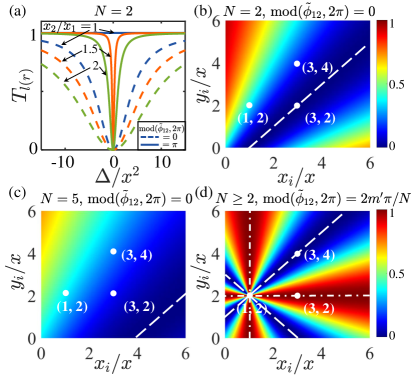
Figure 2: Transmission probabilities $T_{l(r)}$ in the Markovian regime with chiral coupling. (a) $T_{l(r)}$ given by Eq. (24) and Eq. (25) as functions of $\Delta$ by considering $x_{2}/x_{1}=\{1,2,3\}$ with $N=2$ coupling points. The dashed lines correspond to the single-photon transmission spectrum under the condition of $x_{1}+x_{2}=y_{1}+y_{2}$, $\text{mod}(\tilde{\phi}_{12},2\pi)=0$, and the solid lines correspond to $|x_{1}-x_{2}|=|y_{1}-y_{2}|$, $\text{mod}(\tilde{\phi}_{12},2\pi)=\pi$. For $\text{mod}(\tilde{\phi}_{12},2\pi)=\pi$, $T_{l(r)}$ remains unity under the even coupling condition $x_{2}=x_{1}$, while for $x_{2}\neq x_{1}$, $T_{l(r)}$ become the anti-Lorentzian lineshape with a narrow half width $2(x_{1}-x_{2})^{2}$ and undergo a sudden jump from unity to zero at resonance $\Delta=0$. (b)-(d) $T_{l(r)}$ versus the coupling strengths $x_{i}/x$ and $y_{i}/x$ at the the $i$th coupling point with (b) $N=2$, $\text{mod}(\tilde{\phi}_{12},2\pi)=0$, $\Delta=\Delta_{LS}=0$, (c) $N=5$, $\text{mod}(\tilde{\phi}_{12},2\pi)=0$, $\Delta=\Delta_{LS}=0$, and (d) $N\geq 2$, $\text{mod}(\tilde{\phi}_{12},2\pi)=2m^{\text{$\prime$}}\pi/N$, $\Delta=\Delta_{LS}$, respectively. Here, we consider the $N$ coupling points are equally spaced, and set $(x_{j},y_{j})/x=(1,2)$ for $j\neq i$. The white dot-dashed lines indicate $T_{l(r)}=1$ under the condition of unidirectional uneven coupling $x_{i}=x$ or $y_{i}=y$. The white dashed lines correspond to $T_{l(r)}=0$ under the condition of $\Gamma{}_{x}=\Gamma{}_{y}$ with respect to the case of bi-directional uneven coupling, except the point of intersection between the lines. The white dots indicate the three different coupling regimes discussed later.

III photon scattering with chiral coupling: The Markovian regime

By considering the chiral coupling with $\gamma=0$ and assuming $x_{i}$ ($y_{i}$) being positive real values, one typically has $\Gamma_{x}\neq\Gamma_{y}$, i.e., $\frac{1}{2}\sum_{\{i,j\}=1}^{N}(x_{i}x_{j}-y_{i}y_{j})\text{cos}\phi_{ij}\neq 0$. The chirality can be divided into three different regimes: (1) bidirectional even coupling (BEC) $x_{i}=x_{j},y_{i}=y_{j},$ but $x_{i}\neq y_{i}$; (2) unidirectional un-even coupling (UUEC) $x_{i}=x_{j},y_{i}\neq y_{j}$, or $x_{i}\neq x_{j},y_{i}=y_{j}$; (3) bidirectional un-even coupling (BUEC) $x_{i}\neq x_{j},y_{i}\neq y_{j}$. Remarkably, we find that $\Gamma_{x}=\Gamma_{y}$ can be achieved by appropriately tuning the uneven coupling strengths distributed at different coupling points. As a result, it offers a flexible way to control the transmission and reflection of a single incident photon, and allows for in situ photon routing at multiple frequency windows. This will be discussed in detail later.

III.1 Bidirectional even coupling

We first consider the bidirectional even coupling regime for a giant atom with $N\geq 2$ coupling points, where the coupling strengths of the $N$ coupling points are identical for the same propagation direction, and are set to $x_{i}=x$ and $y_{i}=y$. Due to the multiple-point interference effect, the effective Lamb shift in total takes the form

$$\Delta_{LS}=\frac{1}{2}\left(x^{2}+y^{2}\right)\frac{N\text{sin}\tilde{\phi}_{12}-\text{sin}N\tilde{\phi}_{12}}{1-\text{cos}\tilde{\phi}_{12}},$$ (14)

and the sum (difference) of the two effective decay rates is given by

$$\Gamma_{x}\pm\Gamma_{y} = \frac{1}{2}\left(x^{2}\pm y^{2}\right)\frac{\text{sin}^{2}\left(\frac{1}{2}N\tilde{\phi}_{12}\right)}{\text{sin}^{2}\left(\frac{1}{2}\tilde{\phi}_{12}\right)},$$ (15)

which shows that the photon interferes with itself multiple times at the two (left and right) propagation directions independently.

(1) When the propagating phase satisfies $\text{mod}(\tilde{\phi}_{12},2\pi)=0$, the Lamb shift vanishes regardless of the coupling directions, but the effective decay rates are $N^{2}$-enhanced and are given by

$$\Gamma_{x}\pm\Gamma_{y}=\frac{\left(\sum_{i=1}^{N}x_{i}\right)^{2}\pm\left(\sum_{i=1}^{N}y_{i}\right)^{2}}{2}=\frac{1}{2}N^{2}\left(x^{2}\pm y^{2}\right).$$ (16)

The transmission probabilities then read

$$T_{l}=T_{r} = \frac{4\Delta^{2}+N^{4}\left(x^{2}-y^{2}\right)^{2}}{4\Delta^{2}+N^{4}\left(x^{2}+y^{2}\right)^{2}}.$$ (17)

In contrast to the uniformly symmetric coupling case ($x=y$), the chirality leads to a nonvanishing transmission $T_{l(r)}\neq 0$ at resonance $\Delta=0$, i.e.,

$$T_{l(r)}=\left(\frac{\Gamma_{x}-\Gamma_{y}}{\Gamma_{x}+\Gamma_{y}}\right)^{2}=\left(\frac{x^{2}-y^{2}}{x^{2}+y^{2}}\right)^{2},$$ (18)

corresponding to $T_{l(r)}$ in the large $N\rightarrow\infty$ limit.

(2) For $\text{mod}(\tilde{\phi}_{12},2\pi)=2m^{\text{$\prime$}}\pi/N$ ($m^{\text{$\prime$}}=1,2,...,N-1$), the Lamb shift can be nonvanishing and is given by

$$\Delta_{LS}=\frac{N}{2}\left(x^{2}+y^{2}\right)\text{cot}\left(\frac{m^{\text{$\prime$}}\pi}{N}\right),$$ (19)

but the effective decay rates vanish ($\Gamma_{x}=\Gamma_{y}=0$) due to the destructive interference effect among the coupling points, which is analogous to the case with uniformly symmetric coupling, then a photon incident from the left or the right will be completely transmitted, independent of the frequency detuning between photon and atomic transition.

III.2 Unidirectional un-even and bidirectional un-even coupling

The results for the BEC regime can be understood intuitively, but those for the UUEC and the BUEC regimes are not self-evident. To obtain instructive insight, we first consider the simplest model with only $N=2$ coupling points in the Markovian limit, where the Lamb shifts are $\Delta_{x}=\Delta_{y}=0$ both for $\text{mod}(\tilde{\phi}_{12},2\pi)=0$ and $\text{mod}(\tilde{\phi}_{12},2\pi)=2m^{\text{$\prime$}}\pi/N$, but the sum and difference of the two effective decay rates $\Gamma_{x}\pm\Gamma_{y}$ strongly depend on the chirality of the coupling strengths. For $\text{mod}(\tilde{\phi}_{12},2\pi)=0$, the effective decay rates are simply given by

$$\Gamma_{x}\pm\Gamma_{y}=\frac{(x_{1}+x_{2})^{2}\pm(y_{1}+y_{2})^{2}}{2},$$ (20)

and correspondingly the transmission probabilities are

$$T_{l(r)} = \frac{4\Delta^{2}+\left[\left(x_{1}+x_{2}\right)^{2}-\left(y_{1}+y_{2}\right)^{2}\right]^{2}}{4\Delta^{2}+\left[\left(x_{1}+x_{2}\right)^{2}+\left(y_{1}+y_{2}\right)^{2}\right]^{2}};$$ (21)

for $\text{mod}(\tilde{\phi}_{12},2\pi)=\pi$, the effective decay rates are alternatively given by

$$\Gamma_{x}\pm\Gamma_{y} = \frac{(x_{1}-x_{2})^{2}\pm(y_{1}-y_{2})^{2}}{2},$$ (22)

and the transmission probabilities read

$$T_{l(r)}=\frac{4\Delta^{2}+\left[\left(x_{1}-x_{2}\right)^{2}-\left(y_{1}-y_{2}\right)^{2}\right]^{2}}{4\Delta^{2}+\left[\left(x_{1}-x_{2}\right)^{2}+\left(y_{1}-y_{2}\right)^{2}\right]^{2}}.$$ (23)

Note that in the UUEC regime, i.e., $x_{1}=x_{2}$ and $y_{1}\neq y_{2}$ (or $y_{1}=y_{2}$ and $x_{1}\neq x_{2}$), Eq. (21) reduces to

$$T_{l(r)}=\frac{\Delta^{2}}{\Delta^{2}+\left(x_{1}+x_{2}\right)^{4}},$$ (24)

if the coupling strengths satisfy $x_{1}+x_{2}=y_{1}+y_{2}$, which possesses the anti-Lorentzian line shape centered at $\Delta=0$ with the FWHM $2(x_{1}+x_{2})^{2}$ and the minimum $T_{l(r)}(\Delta=0)=0$, in contrast to $0<T_{l(r)}<1$ of the BEC regime, see Fig. 2(a); on the other hand, the transmission probabilities [Eq. (23)] for $\text{mod}(\tilde{\phi}_{12},2\pi)=\pi$ are constant unity (i.e., $T_{l(r)}\equiv 1$) regardless of the specific value of the detuning $\Delta$, exhibiting the same feature as in the BEC regime. In the BUEC regime, the overall profile of $T_{l(r)}$($\Delta$) for $\text{mod}(\tilde{\phi}_{12},2\pi)=0$ is below unity and $T_{l(r)}(\Delta=0)=0$ again for $x_{1}+x_{2}=y_{1}+y_{2}$; while for $\text{mod}(\tilde{\phi}_{12},2\pi)=\pi$, it is remarkable that, under the condition of $|x_{1}-x_{2}|=|y_{1}-y_{2}|$ (corresponding to $\Gamma_{x}=\Gamma_{y}\neq 0$), $T_{l(r)}$($\Delta$) [Eq. (23)] reduce to

$$T_{l(r)}=\frac{\Delta^{2}}{\Delta^{2}+\left(x_{1}-x_{2}\right)^{4}},$$ (25)

which have the minimum $T_{l(r)}(\Delta=0)=0$ at resonance, and possess the FWHM $2(x_{1}-x_{2})^{2}$ that can be infinitely narrow for $x_{2}/x_{1}\rightarrow 1$, in contrast to $T_{l(r)}(\Delta)\equiv 1$ for both the BEC and the UUEC regimes. In other words, an incident photon can be totally reflected or fully transmitted for the "destructive" interference phases $\text{mod}(\tilde{\phi}_{12},2\pi)=\pi$ by modulating the chirality of the coupling strengths, and moreover, the width of the reflection window can be flexibly tuned [as shown in Fig. 2(a)], offering the potential application for sensing and optical switch (Cai and Jia, 2021; Peng and Jia, 2023; Gu et al., 2017).

For $N>2$, we consider the simplified model where the coupling strengths at the $i$th coupling point $x_{i}$ ($y_{i}$) for the left-propagating (right-propagating) photons are uniquely different from that [assumed to be identical to $x$ ($y$)] of all the other ($N-1$) coupling points. A brief calculation shows that the Lamb shift is given by

$$\Delta_{LS}= \frac{x^{2}+y^{2}}{2}\left(NS_{1}-S_{N}\right)-\frac{x(x-x_{i})+y(y-y_{i})}{2}$$

$$\text{$\times$}\left(2S_{1}+S_{i-1}-S_{i}+S_{N-i}-S_{N-i+1}\right),$$ (26)

with $S_{j}(\tilde{\phi}_{12})=\text{sin}(j\tilde{\phi}_{12})/(1-\text{cos}\tilde{\phi}_{12})$, $j\in\mathbf{N}$, and the effective decay rates are

$$\Gamma_{x}\pm\Gamma_{y}= \frac{x^{2}\pm y^{2}}{2}C_{N}+\frac{\left(x-x_{i}\right)^{2}\pm\left(y-y_{i}\right)^{2}}{2}$$

$$+\frac{x\left(x-x_{i}\right)\pm y\left(y-y_{i}\right)}{2}$$

$$\times\left(C_{i-1}-C_{i}+C_{N-i}-C_{N-i+1}\right),$$ (27)

with $C_{j}(\tilde{\phi}_{12})=\text{sin}^{2}\left(\frac{1}{2}j\tilde{\phi}_{12}\right)/\text{sin}^{2}\left(\frac{1}{2}\tilde{\phi}_{12}\right)$. Note that both the Lamb shifts and the decay rates strongly depend on the differences (or chirality) of the coupling strengths $\left(x-x_{i}\right)$ and $\left(y-y_{i}\right)$, and moreover, are related to the specific location of the disorder (i.e., the $i$th coupling point).

(1) Again, the Lamb shifts vanish for $\text{mod}(\tilde{\phi}_{12},2\pi)=0$ due to $S_{j}(\tilde{\phi}_{12})=0$, but the decay rates in Eq. (27) become dependent on the number of the coupling points according to

$$\Gamma_{x}\pm\Gamma_{y}=\frac{\left[\left(N-1\right)x+x_{i}\right]^{2}\pm\left[\left(N-1\right)y+y_{i}\right]^{2}}{2}.$$ (28)

It follows that the transmission probabilities are

$$T_{l(r)}=\frac{4\Delta^{2}+\left\{\left[\left(N-1\right)x+x_{i}\right]^{2}-\left[\left(N-1\right)y+y_{i}\right]^{2}\right\}^{2}}{4\Delta^{2}+\left\{\left[\left(N-1\right)x+x_{i}\right]^{2}+\left[\left(N-1\right)y+y_{i}\right]^{2}\right\}^{2}},$$ (29)

and thus, the incident photon is totally reflected at $\Delta=0$ if the chirality of the coupling strengths satisfies

$$\left(N-1\right)x+x_{i}=\left(N-1\right)y+y_{i},$$ (30)

which reduces to $x+x_{i}=y+y_{i}$ for $N=2$ as discussed before. In Fig. 2(b) [Fig. 2(c)], we show $T_{l(r)}[\Delta=0,\text{mod}(\tilde{\phi}_{12},2\pi)=0]$ as functions of $x_{i}$ and $y_{i}$ (in units of $x$) with $y/x=2$ and $N=2$ ($N=5$), and indicate $T_{l(r)}=0$ (or $R_{l(r)}=1$) corresponding to the condition [Eq. (30)] by white dashed lines. Around the resonance, $T_{l(r)}(\Delta)$ under the condition of Eq. (30) possess the anti-Lorentzian line shape with the FWHM $2\left[\left(N-1\right)x+x_{i}\right]^{2}$ scaling as $N^{2}$.

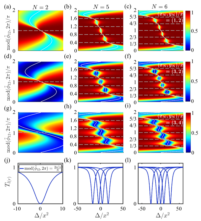
Figure 3: Transmission probabilities $T_{l(r)}$ versus $\Delta$ and $\text{mod}(\tilde{\phi}_{12},2\pi)$ for $N=2$, 5, 6, respectively. We consider the rightmost (i.e., $N$th) coupling point which has the coupling strengths $(x_{N},y_{N})/x$ different to that of the others with $(x_{j},y_{j})/x=(1,2)$ ($j\neq N$). As indicated in Fig. 2(d), we set $(x_{N},y_{N})/x=\{(1,2),(3,2),(3,4)\}$, which (from top to bottom) correspond to the BEC [(a)-(c)], the UUEC [(d)-(f)], and the BUEC [(g)-(i)] regime, respectively. The white solid lines are used to label the solutions for $\Delta=\Delta_{LS}(\tilde{\phi}_{12})$, and the horizontal gray dashed lines label the phases $\text{mod}(\tilde{\phi}_{12},2\pi)=2m^{\text{$\prime$}}\pi/N$ ($m^{\text{$\prime$}}=1,2,...,N-1$). Panels (j)-(l) depict transmission spectrum in the BUEC regime by fixing $\text{mod}(\tilde{\phi}_{12},2\pi)=2m^{\text{$\prime$}}\pi/N$, where specially for $N$ being an even number, one can observe $T_{l(r)}=0$ at the resonance $\Delta=0$ with $N-2$ dips symmetrically around it.

(2) For $\text{mod}(\tilde{\phi}_{12},2\pi)=2m^{\text{$\prime$}}\pi/N$, there exist the mathematical identities $C_{j}(\tilde{\phi}_{12})=C_{N-j}(\tilde{\phi}_{12})$ and $S_{j}\left(\tilde{\phi}_{12}\right)=-S_{N-j}\left(\tilde{\phi}_{12}\right)$ ($j=0,1,...,N$), from which we readily find the Lamb shifts being nonvanishing and $N$-dependent

$$\Delta_{LS}= NS_{1}\frac{x^{2}+y^{2}}{2}-\left(S_{1}+S_{i-1}-S_{i}\right)$$

$$\times\left[x(x-x_{i})+y(y-y_{i})\right],$$ (31)

and more interestingly, the $N$-independent effective decay rates

$$\Gamma_{x}\pm\Gamma_{y}=\frac{1}{2}\left[(x-x_{i})^{2}\pm(y-y_{i})^{2}\right].$$ (32)

In analogy to the case of $N=2$, $\Gamma_{x}\pm\Gamma_{y}$ are simply determined by the chirality of the coupling strengths $\left(x-x_{i}\right)$ and $\left(y-y_{i}\right)$. As a result, an incident photon is perfectly transmitted [$T_{l(r)}(\Delta)\equiv 1$] if $x=x_{i}$ or $y=y_{i}$, regardless of the specific value of the detuning $\Delta$. In the BUEC regime, when the coupling strengths of the disordered coupling point fulfill the condition

$$|x-x_{i}|=|y-y_{i}|,$$ (33)

the transmission probabilities reduce to

$$T_{l(r)}=\frac{\left(\Delta-\Delta_{LS}\right)^{2}}{\left(\Delta-\Delta_{LS}\right)^{2}+\left(x-x_{i}\right)^{4}},$$ (34)

which again possess the anti-Lorentzian line shape of the tunable width $2(x-x_{i})^{2}$ but with the center ($T_{l(r)}=0$) shifted to $\Delta=\Delta_{LS}$. In Fig. 2(d), we have shown the density plot of $T_{l(r)}(\Delta=\Delta_{LS})$ as functions of the chiral coupling $(x_{j},y_{j})/x$, and indicated the UUEC regime by horizontal and vertical dot-dashed lines and the BUEC regime with $|x-x_{i}|=|y-y_{i}|$ by white dashed line. The intersection of the white dashed line with the coordinate $(x_{j},y_{j})/x=(1,1)$ corresponds to the BEC regime with $T_{l(r)}=1$. Furthermore, if we take $i=N$, i.e., the coupling strength of the leftmost (or rightmost) is different from that of the others, Eq. (31) then reduces to $\Delta_{LS}=\frac{N}{2}\left(x^{2}+y^{2}\right)\text{cot}(m^{\text{$\prime$}}\pi/N)$, which is exactly the same to that of the BEC regime, see Eq. (19). Note that $\Delta_{LS}$ is now independent of the coupling strengths {$x_{N}$, $y_{N}$} at the $N$th coupling point, therefore, by engineering the chirality of the disordered coupling point, the transmission probabilities $T_{l(r)}(\Delta)$ can be tuned from zero to unity in situ at $\Delta=\frac{N}{2}\left(x^{2}+y^{2}\right)\text{cot}(m^{\text{$\prime$}}\pi/N)$ with $m^{\text{$\prime$}}=1,2,...,N-1$, and the width of the transmission window given by $2(x-x_{N})^{2}$ can be flexibly controlled.

In Fig. 3, we plot the transmission probabilities $T_{l(r)}$ as functions of the detuning $\Delta$ and the two-point phase delay $\tilde{\phi}_{12}$ modulo $2\pi$ [i.e., $\text{mod}(\tilde{\phi}_{12},2\pi)$] with $y/x=2$ and $N=\{2,5,6$}. We consider the set of coupling strengths $(x_{N},y_{N})/x=\{(1,2),(3,2),(3,4)\}$ for the disordered (or the $N$th) coupling point, corresponding to the BEC, the UUEC, and the BUEC regime, respectively. We first look at the case of $N=2$ shown in Fig. 3(a), (d) and (g), for $\text{mod}(\tilde{\phi}_{12},2\pi)=0$, the incident photon is partially reflected (i.e., $0<T_{l(r)}<1$) in the BEC regime with $\text{(}x_{N},y_{N})/x=(1,2)$, and nevertheless is totally reflected (i.e $T_{l(r)}=0$) in the UUEC regime with $\text{(}x_{N},y_{N})/x=(3,2)$ (satisfying $x+x_{i}=y+y_{i}$). In both cases, the incident photon will be completely transmitted for $\text{mod}(\tilde{\phi}_{12},2\pi)=\pi$, which are indicated by the gray dashed line. As a result, the two red regions (corresponding to high transmission probabilities), that are divided by the white solid line with regard to the condition $\Delta=\Delta_{LS}(\tilde{\phi}_{12})$, connect to each other around $\Delta=0$. In contrast, in the BUEC regime with $\text{(}x_{N},y_{N})/x=(3,4)$ (satisfying $|x-x_{i}|=|y-y_{i}|$), there appears a blue channel that separates the two high transmission regions and has the minimum $T_{l(r)}=0$ precisely at $\Delta=0$ with $\text{mod}(\tilde{\phi}_{12},2\pi)=\pi$. Extending the results to $N=5$ ($N=6)$ and comparing them of the three regimes, we then find $N-1$ “total reflection windows” at $\Delta\sim\Delta_{LS}=\frac{N}{2}\left(x^{2}+y^{2}\right)\text{cot}(\tilde{\phi}_{12}/2)$ with $\text{mod}(\tilde{\phi}_{12},2\pi)=2m^{\text{$\prime$}}\pi/N$ ($m^{\text{$\prime$}}=1,2,...,N-1$) in the BUEC regime, and the opened channels connect the $N$ disjunct blue regions for the BEC and the UUEC regimes. Moreover, the transmission spectrum along $\text{mod}(\tilde{\phi}_{12},2\pi)=2m^{\text{$\prime$}}\pi/N$ (indicated by the horizontal dashed lines) possess the anti-Lorentzian lineshape centered at $\Delta=\Delta_{LS}$ with tunable width [see Figs. 3(j), (k) and (l)]. It is worth noting that $\Delta_{LS}$ is independent of the specific values of the coupling strengths $(x_{i},y_{i})$ for $i=N$, thus, by setting $\Delta=\Delta_{LS}(\tilde{\phi}_{12}=\frac{2m^{\prime}\pi}{N})$, the setup can potentially act as a multi-channel photon router, with the frequencies of incident photons $\omega_{e}+\Delta_{LS}(\tilde{\phi}_{12})$ and the number of channels $N-1$ under the condition of $\text{mod}(\tilde{\phi}_{12},2\pi)\in(0,2\pi)$.

IV Nonreciprocal photon scattering with atomic spontaneous emission

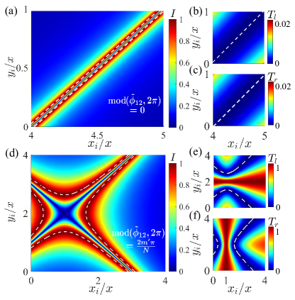
Figure 4: Nonreciprocal transport of a single photon by including the spontaneous emission decay $\gamma/x^{2}=0.2$. The contrast ratio $I$ versus $x_{i}/x$ and $y_{i}/x$ for (a) $N=5$, $\text{mod}(\tilde{\phi}_{12},2\pi)=pi$ and (d) $N\geq 2$, $\text{mod}(\tilde{\phi}_{12},2\pi)=2m^{\text{$\prime$}}\pi/N$, with the corresponding transmission probability $T_{l}$ ($T_{r}$) for a left-incident (right-incident) photon being shown in (b) [(c)] and (e) [(f)]. The white dashed lines in panels (a), (d) indicate the optimal nonreciprocity condition with $I=1$. The white hyperbola dashed lines in (b) [(c)] and (e) [(f)] are used to label the transmission probabilities with $T_{l(r)}=0$, corresponding to $\gamma+\Gamma_{x}=\Gamma_{y}$ or $\gamma+\Gamma_{y}=\Gamma_{x}$. Other parameters are the same as in Figs. 2 (c)-(d).

We now take the atomic spontaneous decay into account, i.e., $\gamma\neq 0$. Previously, we mentioned that nonreciprocal photon scattering (i.e., $T_{l}\neq T_{r}$) can not occur for the giant atom with uniformly symmetric coupling. Moreover, it is remarkable that only reciprocal photon transport can be observed with $\gamma=0$ despite the even or uneven chiral coupling. However, we will see that, by engineering the chirality of the coupling strengths, nonreciprocal photon transfer can be realized, due to the joint effect of the chirality (i.e., $\Gamma_{x}\neq\Gamma_{y}$) and the atomic spontaneous decay $\gamma\neq 0$, and while the reflections are reciprocal $R_{l}=R_{r}$, see Eqs. (6) and (7). In other words, the atomic spontaneous decay of the giant atom due to its coupling to the thermal environment and the external decay due to the interfaced waveguide can cooperatively lead to nonreciprocal photon transport.

As an example, for $\gamma=\Gamma_{x}-\Gamma_{y}$ and $\Delta=\Delta_{LS}$, a photon incident from the left will be partially transmitted with the probability

$$T_{l}=\left(1-\frac{\Gamma_{y}}{\Gamma_{x}}\right)^{2},$$ (35)

while a photon incident from the right will be completely isolated, i.e., $\text{ $T_{r}$}=0$. For a generic situation, the nonreciprocity in transmission can be described by a contrast ratio defined as

$$I=\left|\frac{T_{l}-T_{r}}{T_{l}+T_{r}}\right|=\frac{2\gamma\left|\Gamma_{x}-\Gamma_{y}\right|}{\left(\Delta-\Delta_{LS}\right)^{2}+\gamma^{2}+\left(\Gamma_{x}-\Gamma_{y}\right)^{2}}.$$ (36)

Thus, the nonreciprocity can only be observed when both the conditions $\gamma\neq 0$ and $\Gamma_{x}\neq\Gamma_{y}$ are simultaneously satisfied. By setting $\Delta=\Delta_{LS}$, one achieves the optimal nonreciprocity $I=1$ with $\gamma=|\Gamma_{x}-\Gamma_{y}|,$ where the spontaneous decay rate $\gamma$ cancels out the difference between the effective decay rates in the forward and backward direction. For $\Delta\neq\Delta_{LS}$, the contrast ratio is always less than one.

In Figs. 4(a) and 4(d), we plot the contrast ratio $I$ as functions of the coupling strengths $(x_{i},y_{i})/x$ for $y/x=2$, $\gamma/x^{2}=0.2$, (a)-(c) $N=5$, and (d)-(f) $N\geq 2$. Correspondingly, we show the forward (backward) transmission probabilities $T_{l}(\Delta=\Delta_{LS})$ [$T_{r}(\Delta=\Delta_{LS})$] for a left-incident (right-incident) photon in Figs. 4(b)-4(c) with $\text{mod}(\tilde{\phi}_{12},2\pi)=0$ and Figs. 4(e)-4(f) with $\text{mod}(\tilde{\phi}_{12},2\pi)=2m^{\text{$\prime$}}\pi/N$. As discussed above, the optimal nonreciprocity ($I=1$) condition for $\text{mod}(\tilde{\phi}_{12},2\pi)=0$ is

$$\gamma=\pm\frac{\left[\left(N-1\right)x+x_{i}\right]^{2}-\left[\left(N-1\right)y+y_{i}\right]^{2}}{2},$$ (37)

and alternatively for $\text{mod}(\tilde{\phi}_{12},2\pi)=2m^{\text{$\prime$}}\pi/N$ ($m^{\text{$\prime$}}=1,2,...,N-1$) is

$$\gamma=\pm\frac{\left(x_{i}-x\right)^{2}-\left(y_{i}-y\right)^{2}}{2},$$ (38)

corresponding to the hyperbola branches indicated by the white dashed lines in Fig. 4(a) and Fig. 4(d). Note that for $\text{mod}(\tilde{\phi}_{12},2\pi)=0$, one can only observe the tail of hyperbola branches since we consider the coupling strengths being positive values; when physical parameters (coupling strengths) are extended to the complex plane, the full hyperbola branches will be clearly seen in the lower left quadrant. However, the optimal nonreciprocity is achieved at the expense of low transmission probabilities $T_{l(r)}$ [shown in Fig. 4(b) and Fig. 4(c)]. For $\text{mod}(\tilde{\phi}_{12},2\pi)=2m^{\text{$\prime$}}\pi/N$, we previously show in the UUEC regime $T_{l}=T_{r}\equiv 1$ along $y_{i}/y=1$ ($x_{i}/x=1$) for $\gamma=0$, in contrast to that, when $\gamma\neq 0$, there emerges an avoided crossing at the BEC point $(x_{i},y_{i})/x=(1,2)$ with a gap $\sim 2\sqrt{2\gamma}$ of the coupling strength $y_{i}/y$ ($x_{i}/x$) for $T_{l}$ ($T_{r}$) in Fig. 4(e) [Fig. 4(f)]. Here, the optimal nonreciprocity [Eq. (38)] corresponds to the total reflection of the incident photon $T_{l}=0$ or $T_{r}=0$, as indicated by the white dashed lines in Fig. 4(e) and Fig. 4(f). In particular, by considering the UUEC regime (i.e., $\Gamma_{x}=0$ or $\Gamma_{y}=0$), we obtain the optimal nonreciprocity $I=1$ with $T_{l}=0$ ($T_{r}=1)$ or $T_{l}=1$ ($T_{r}=0)$ for a left-incident (right-incident) photon, since the chiral coupling $y_{i}$ ($x_{i}$) at the $i$th coupling point is counteracted by the spontaneous decay according to $y_{i}=y\pm\sqrt{2\gamma}$ ($x_{i}=x\pm\sqrt{2\gamma}$). Extending to a generic picture including the BUEC regime, one finally observes $I=1$ on the hyperbola branches in Fig. 4(d).

V The Non-Markovian regime

So far, we consider only the Markovian regime, namely, the time for light to travel between the leftmost and the rightmost coupling points is much less than the characteristic relaxation time $\tau_{1N}\ll\tilde{\Gamma}^{-1}$. For the giant atom with $N$ equally spaced coupling points, where $\tilde{\Gamma}$ is on the same order of $N^{2}x^{2}$ (with regard to the uniformly symmetric coupling) (Guo et al., 2017; Cai and Jia, 2021; Ask et al., 2019), the system in the non-Markovian regime implies $\tau_{1N}=(N-1)\tau_{12}$ being comparable to or even larger than $\tilde{\Gamma}^{-1}$. Moreover, by considering the bandwidth of the order $|\Delta|\sim\tilde{\Gamma}$ or $|\Delta|/x^{2}\sim N^{2}$, the effect of $\Delta\tau_{12}$ on the propagating phase $\phi_{12}=\Delta\tau_{12}+\tilde{\phi}_{12}$ (and therefore the non-Markovian retardation effect) can not be ignored (Du et al., 2021; Zhou et al., 2023).

In Fig. 5, we show transmission spectra for $N=2$ coupling points as functions of $\Delta/x^{2}$ for $x^{2}\tau_{12}=0.25,1,2.5$, respectively. We consider the set of coupling strengths with $(x_{1},y_{1},x_{2},y_{2})/x=(1,0.5,1,0.5)$, $(x_{1},y_{1},x_{2},y_{2})/x=(1,0.5,1,1.5)$, and $(x_{1},y_{1},x_{2},y_{2})/x=(1,0.5,0.5,1)$, according to the specific chiral conditions Eqs. (30) and (33). For $x^{2}\tau_{12}=0.25$, the weak non-Markovian effect starts to influence the transmission spectra. For $\text{mod}(\tilde{\phi}_{12},2\pi)=0$, all of the scattering spectrum have a single minimum at $\Delta=0$ but with a different width for different chiral coupling strengths. For $\text{mod}(\tilde{\phi}_{12},2\pi)=\pi$, the transmission probabilities in the UUEC [with $(x_{1},y_{1},x_{2},y_{2})/x=(1,0.5,1,1.5)$] and the BEC [with $(x_{1},y_{1},x_{2},y_{2})/x=(1,0.5,1,0.5)$] regime decline weakly from $T_{l(r)}(\Delta=0)=1$ as $\Delta$ increases, while in the BUEC regime [with $(x_{1},y_{1},x_{2},y_{2})/x=(1,0.5,0.5,1)$], $T_{l(r)}(\Delta)$ quickly transits from zero to almost one for being out of resonance [see Fig. 5(b)]. For $x^{2}\tau_{12}=1$, the system enters the intermediate non-Markovian regime. For $\text{mod}(\tilde{\phi}_{12},2\pi)=0$, there emerges a frequency window with the transmission probabilities approximately unchanged, and in particular, $T_{l(r)}$ remain zero in the frequency window for the BUEC regime, which is referred to as a photonic band gap with $|\Delta|/x^{2}\propto N^{2}$ (Cai and Jia, 2021); for $\text{mod}(\tilde{\phi}_{12},2\pi)=\pi$, $T_{l(r)}$ start to oscillate with additional minima. In the deep non-Markovian regime with $x^{2}\tau_{12}=2.5$ and $\text{mod}(\tilde{\phi}_{12},2\pi)=0$, the flat band structure splits and exhibits side valleys, and only in the case with respect to the BUEC regime, we observe $T_{l(r)}=0$ at the two side valleys close to $\Delta=0$. As $\Delta$ increases, $T_{l(r)}(\Delta)$ in the BEC and the BUEC regimes then oscillate between zero and one both for $\text{mod}(\tilde{\phi}_{12},2\pi)=\pi$ and $\text{mod}(\tilde{\phi}_{12},2\pi)=0$.

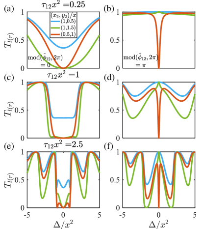
Figure 5: Transmission spectra in the non-Markovian regime with $N=2$ and $\gamma=0$, where (a), (c), (e) $\text{mod}(\tilde{\phi}_{12},2\pi)=0$ (the left panels), and (b), (d), (f) $\text{mod}(\tilde{\phi}_{12},2\pi)=\pi$ (the right panels). The photon propagation time is set as $x^{2}\tau_{12}=\{0.25,1,2.5\}$, corresponding to the weak, intermediate, and deep non-Markovian regimes, respectively. Coupling strengths for the two coupling points are $(x_{1},y_{1},x_{2},y_{2})/x=\{(1,0.5,1,0.5),(1,0.5,1,1.5),(1,0.5,0.5,1)\}$, which correspond to the BEC (blue), the UUEC (green), and the BUEC (red) regime, respectively.

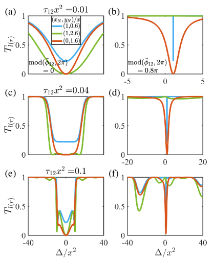
Figure 6: Transmission spectrum in the non-Markovian regime with $N=5$ and $\gamma=0$, where (a), (c), (e) $\text{mod}(\tilde{\phi}_{12},2\pi)=0$, and (b), (d), (f) $\text{mod}(\tilde{\phi}_{12},2\pi)=0.8\pi$ [i.e., $\text{mod}(\tilde{\phi}_{12},2\pi)=2m^{\text{$\prime$}}\pi/N$ with $m^{\text{$\prime$}}=2$ without loss of generality]. We set the coupling strengths of the $N$th coupling point as $(x_{N},y_{N})/x=\{(1,0.6),(1,2.6),(0,1.6)\}$ and that of the others as $(x_{j},y_{j})/x=(1,0.6)$ ($j\neq N$), which correspond to the BEC (blue), the UUEC (green), and the BUEC (red) regime, respectively. Moreover, the photon propagation time is set as $x^{2}\tau_{12}=\{0.01,0.04,0.1\}$, corresponding to the weak, intermediate, and deep non-Markovian regimes, respectively.

In Fig. 6, we show the transmission spectra as functions of $\Delta/x^{2}$ with $N=5$ for $x^{2}\tau_{12}=0.01,0.04,\text{ and }0.1$, respectively. We consider the propagating time $\tau_{1N}\sim\left(N^{2}x^{2}\right)^{-1}$ from the first to the last coupling point, and the frequency bandwidth $|\Delta|\sim N^{2}x^{2}$. The disordered coupling point locates at the $N$th coupling point with $(x_{N},y_{N})/x=(0,0.6)$ and $(x_{N},y_{N})/x=(1,2.6)$, and the coupling strengths for the other coupling points are $(x_{j},y_{j})/x=(1,0.6)$, corresponding to the BUEC and the UUEC regimes respectively. Moreover, the coupling strengths $(x_{N},y_{N})/x=(0,0.6)$ satisfy both the conditions $x_{N}-y_{N}=\left(1-N\right)\left(x-y\right)$ and $|x_{N}-x|=|y-y_{N}$|, while the coupling strengths $(x_{N},y_{N})/x=(1,2.6)$ satisfy $x_{N}-y_{N}=\left(1-N\right)\left(x-y\right)$ only. For $\text{mod}(\tilde{\phi}_{12},2\pi)=0$, the transmission spectra in the three regimes $x^{2}\tau_{12}=\{0.01,0.04,0.1\}$ all show similar features to that of $N=2$. In the intermediate and deep non-Markovian regimes, the transmission probabilities saturate to unity after a few oscillations as $\Delta$ increases, see Figs. 6(a), 6(c) and 6(e). For $\text{mod}(\tilde{\phi}_{12},2\pi)=2m^{\text{$\prime$}}\pi/N$, the lineshape of the scattering spectra becomes asymmetric due to an odd number of coupling points, see Figs. 6(b), 6(d) and 6(f), where we take $m^{\text{$\prime$}}=2$ [i.e., $\text{mod}(\tilde{\phi}_{12},2\pi)=0.8\pi$] as an example. In particular, since the Lamb shift $\Delta_{LS}$ is nonvanishing for $\text{mod}(\tilde{\phi}_{12},2\pi)=2m^{\text{$\prime$}}\pi/N$, the time delay $\sim\Delta\tau_{12}$ will lead to a shift of the dip (with respect to $T_{l(r)}\approx 0$) for the BUEC regime [i.e., $(x_{N},y_{N})/x=(0,0.6)$], while in comparison, the transmission probabilities remain unity at resonance [i.e., $T_{l(r)}(\Delta=0)\equiv 1$] for the UUEC [$(x_{N},y_{N})/x=(1,2.6)$] and the BEC [$(x_{N},y_{N})/x=(1,0.6)$] regimes. Remarkably, since there may not exist an appropriate detuning $\Delta$ fulfilling both $\Gamma_{x}=\Gamma_{y}$ and $\Delta=\Delta_{LS}$, the transmission probability for the BEC regime suffers from a sudden jump to $T_{l(r)}(\Delta_{LS})=\left[(\Gamma_{x}-\Gamma_{y})/(\Gamma_{x}+\Gamma_{y})\right]^{2}$ as $\Delta$ increases [see blue curve in Figs. 6(b), 6(d), and 6(f)]. In general for $\text{mod}(\tilde{\phi}_{12},2\pi)=2m^{\text{$\prime$}}\pi/N$, $T_{l(r)}(\Delta)$ gradually decline in a oscillatory pattern as $\Delta$ increases in the UUEC [$(x_{N},y_{N})/x=(1,2.6)$] and the BEC [$(x_{N},y_{N})/x=(1,0.6)$] regimes, and moreover $T_{l(r)}(\Delta)$ is nonvanishing even at $\Delta=\Delta_{LS}$ for the BUEC regime $\{x_{N},y_{N}\}/x=(0,0.6)$. These phenomena become more obvious as the system enters the intermediate and deep non-Markovian regimes.

VI CONCLUSION

In conclusion, we have studied the photon scattering spectra by a giant atom, which is chirally coupled to a waveguide at multiple equally spaced points. The chirality is categorized in terms of the evenness of coupling strengths in the left and right propagation directions, and is divided into three regimes, i.e., the BEC, the UUEC, and the BUEC regimes. In the Markovian limit and for the two-point propagating phase being $\text{mod}(\tilde{\phi}_{12},2\pi)=0$, the transmission spectra possess the anti-Lorentzian line shape centered at $\Delta=\Delta_{LS}$ for all three regimes, where the incident photon can be totally reflected when the chiral coupling satisfies certain conditions related to the number of coupling points; for the two-point propagating phase satisfying mod($\tilde{\phi}_{12},2\pi)=2m^{\prime}\pi/N$, the incident photon is fully transmitted at $\Delta=\Delta_{LS}$ in the BEC and the UUEC regimes, but can be totally reflected in the BUEC regime by simply modulating the coupling strengths at any one of the coupling points, where, interestingly, a controllable single-photon routing can be implemented in situ at a multiple of frequency “windows”. The photon transport can become nonreciprocal if the atomic spontaneous decay is taken into account, and the nonreciprocity represented by the contrast ratio can be varied from zero to one by engineering the chirality in atom-waveguide couplings, differing from the non-Markovianity induced effect in chiral waveguide QED systems (Du et al., 2021; Zhou et al., 2023). The non-Markovian retardation effect manifested by the scattering spectra reflects itself mainly in the photonic band gap and the oscillatory behavior between total reflection and full transmission, especially in the intermediate and the deep non-Markovian regimes, respectively. The giant-atom-waveguide system with chiral coupling thus offers flexible ways for single-photon routing.