Quantum Bayes Classifiers and Their Application in Image Classification

Abstract

Bayesian networks are powerful tools for probabilistic analysis and have been widely used in machine learning and data science. Unlike the parameters learning mode of neural networks, Bayes classifiers only use sample features to determine the classification results without a time-consuming training process. We study the construction of quantum Bayes classifiers (QBCs) and design a naïve QBC and three semi-naïve QBCs (SN-QBCs). These QBCs are applied to image classification. A local features sampling method is employed to extract a limited number of features from images to reduce the computational complexity. These features are then used to construct Bayesian networks and generate QBCs. We simulate these QBCs on the MindQuantum quantum platform and test them on the MNIST and Fashion-MNIST datasets. Results show that these QBCs based on a limited number of features exhibit good classification accuracies. The classification accuracies of QBCs on the MNIST dataset surpass that of the classical Bayesian network and quantum neural networks that utilize all feature points.

I Introduction

As a tool for studying causal relationships between variables and inferring the impact of variable states on outcomes, Bayesian networks are widely used in various fields such as machine learning and data science, including Monte Carlo analysis MosegaardSambridge-426 , reliability and risk analysis ModarresGroth-449 , health monitoring Daniels-420 , healthcare GaryJarrett-422 , and biomedical systems WongLin-428 . The size of a Bayesian network depends on the number of nodes and the dependencies among them Kwisthout-427 , and learning and inference in large networks can be challenging. Large-scale Bayesian networks have been proven to be an NP-hard problem ChickeringHeckerman-421 . The emergence of quantum computing has provided a new solution to this problem.

In recent years, many quantum algorithms have demonstrated certain advantages over classical computation, providing acceleration in comparison. For example, the Shor’s algorithm Shor-97 achieves exponential acceleration compared to classical computation in solving the problem of factorizing large numbers. The Grover’s algorithm Grover-225 achieves quadratic acceleration in unstructured search. In addition, quantum algorithms based on classical machine learning, such as quantum support vector machine RebentrostMohseni-82 and quantum $K$-nearest neighbor DangJiang-419 , also demonstrate quantum acceleration properties. Image classification is a fundamental problem in computer vision. In recent years, several quantum machine learning models have been used for image classification. These models include quantum convolutional neural networks CongChoi-181 ; KerenidisLandman-432 ; HurKim-435 ; GongPei-455 , quantum $K$-nearest neighbor algorithm DangJiang-419 , and quantum ensemble methods SchuldPetruccione-326 ; MacalusoClissa-437 ; AraujoDaSilva-438 ; MacalusoLodi-431 ; ZhangWang-409 , etc.

Quantum Bayesian networks (QBN) were introduced in 1995 as a simulation of classical ones Youssef-442 . In 2013, Ozols et al. proposed a quantum version of the rejection sampling algorithm called quantum rejection sampling for Bayesian inference OzolsRoetteler-445 . In 2016, Moreira and Wichert proposed a quantum-like Bayesian network that uses amplitudes to represent marginal and conditional probabilities MoreiraWichert-448 . In 2019, Woerner and Egger developed a quantum algorithm WoernerJ-446 for risk analysis using the principles of amplitude amplification and estimation. Their algorithm can provide a quadratic speed-up compared to classical Monte Carlo methods. In 2021, Borujeni et al. proposed a quantum circuit representation of Bayesian networks BorujeniNannapaneni-433 . They designed quantum Bayesian networks for specific problems, such as stock prediction and liquidity risk assessment.

Different from the parameters learning mode of neural networks, Bayesian classification makes a classification decisions based only on sample features, without the tedious training process, resulting in lower computational complexity, faster speed, and less resource consumption. Currently, there is a lack of research on quantum Bayes classifiers (QBCs) building on Bayesian networks for image classification tasks. This paper studies QBCs for image classification. We design a naïve RishOthers-411 ; Leung-429 QBC and three semi-naïve QBCs (SN-QBCs), i.e., the SN-QBC based on SPODE network Kononenko-450 ; Zhou-423 with the feature in the center of an image as the superfather, the SN-QBC based on TAN network Kononenko-450 ; Zhou-423 , and the SN-QBC based on symmetric relationship of features in images. These QBCs are implemented using the MindQuantum Platform Mindquantum-418 , and the classification effects of QBCs are verified on the MNIST LecunBottou-417 and the Fashion-MNIST XiaoRasul-416 datasets.

This paper is organized as follows. Sect. 2 introduces the basic knowledge of Bayes classifiers. Sect. 3 discusses the constructions of QBCs. Sect. 4 presents the image classification algorithm based on QBCs. Sect. 5 demonstrates the simulation results of QBCs for image classification on the MNIST and Fashion-MNIST datasets. Sect. 6 further discusses and concludes the paper.

II Bayes classifier

A Bayes classifier is a statistical classifier based on Bayes’ theorem. It considers selecting the optimal category label based on probabilities and misclassification losses, assuming that all relevant probabilities are known. Suppose the feature of a sample data is $X=\{x_{1},x_{2},\cdots,x_{n}\}$, and the set of class labels is $Y=\{y_{1},y_{2},\cdots,x_{N}\}$. Based on the posterior probability $P(y_{i}|X)$, the expected loss of classifying the sample with feature $X$ as $y_{i}$ is defined as Zhou-423

$$R(y_{i}|X)=\sum_{j=1}^{N}\lambda_{ij}P(y_{j}|X),$$ (1)

where $\lambda_{ij}$ is the misclassification loss. The Bayes classifier attempts to correctly classify new samples with minimal misclassification loss based on the distribution pattern of existing samples. The optimal Bayes classifier can be denoted as

$$D(X)=\arg\min\limits_{y\in Y}R(y|X).$$ (2)

For a specific problem, the misclassification loss $\lambda_{ij}$ can be written as

$$\lambda_{ij}=\begin{cases}0,&\text{if}\ i=j;\\ 1,&\text{otherwise.}\end{cases}$$ (3)

Therefore, the optimal Bayes classifier can be rewritten as

$$D(X)=\arg\max\limits_{y\in Y}P(y|X).$$ (4)

The optimal Bayes classifier selects the class that maximizes the posterior probability $P(y|X)$ given the sample $X$.

Obtaining an accurate posterior probability $P(y|X)$ is important, but in reality, this value is often challenging to obtain. In the probability framework, the posterior probability $P(y|X)$ can be estimated based on a finite training sample. According to Bayes’ theorem Zhou-423 , the posterior probability $P(y|X)$ can be written as

$$P(y|X)=\frac{P(X|y)P(y)}{P(X)},$$ (5)

where $P(X)$ is the evidence factor used for normalization, $P(y)$ is the class-prior probability, and $P(X|y)$ is the class-conditional probability of the sample $X$ with respect to $y$. According to the law of large numbers Offmann-RgensenPisier-451 , when there are a sufficient number of independently and identically distributed samples, $P(y)$ can be estimated by the frequency of each class that appears in the sample. As for the class-conditional probability $P(X|y)$, it involves combinations of all features in $X$. Assuming each feature $x_{i}$ has $d$ possible values, $P(X|y)$ will have $N*d^{n}$ possible values.

II.1 Naïve Bayes Classifier

Clearly, it is difficult to directly obtain the class-conditional probabilities from a limited training sample, as it will result in the problem of combinatorial explosion in calculation, which becomes more severe with the increase of features. The naïve Bayes classifier RishOthers-411 ; Leung-429 is based on the assumption of “independence”, which assumes that each attribute independently affects the classification result, as shown in Fig. (1a). In this case, Eq. (5) can be rewritten as

$$P(y|X)=\frac{P(y)\prod_{i}^{n}P(x_{i}|y)}{P(X)},$$ (6)

where $x_{i}$ the $i$-th attribute of $X$. Since all $P(X)$ are the same, the naïve Bayes classifier can be represented as

$$D_{\text{nb}}=\arg\max\limits_{y\in Y}P(y)\prod_{i}^{n}P(x_{i}|y).$$ (7)

II.2 Semi-naïve Bayes Classifier

The premise of the naïve Bayes classifier is that the features satisfy the assumption of independence, but this is often not the case in practical applications. Therefore, the learning method of the semi-naïve Bayes classifier Kononenko-450 ; Zhou-423 has emerged. It properly considers the dependencies between certain features, which helps to avoid the problem of combinatorial explosion caused by considering the joint probability distribution. Additionally, it takes into account stronger feature dependencies. One-Dependent Estimator (ODE) is the most common strategy for the semi-naïve Bayes classifier, which assumes that each feature only depends on at most one other feature besides the label $y$, that is,

$$P(y|X)\propto P(y)\prod_{i}^{n}P(x_{i}|y,pa_{i}),$$ (8)

where $pa_{i}$ is the dependent feature (or parent feature) of $x_{i}$. The key problem of the semi-naïve Bayes classifier is how to determine the parent feature of feature $x_{i}$.

A typical approach is to assume that all features depend on the same feature, known as the Super-Parent ODE (SPODE), whose dependency relationship is shown in Fig. (1b). Another approach is the Tree Augmented Naïve Bayes (TAN), which computes the conditional mutual information between any pair of features and constructs a maximum weighted tree Camerini-452 ; Zhou-423 based on the feature dependencies, as shown in Fig. (1c).

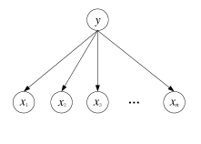
(a) Naïve.

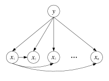
(b) SPODE.

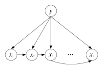
(c) TAN.

Figure 1: Bayesian networks.

III Quantum Bayes classifiers

Unlike classical bits that can only represent either 0 or 1, a quantum bit (qubit) can represent both 0 and 1 simultaneously, i.e., quantum superposition. A single qubit state can be represented as $\ket{\varphi}=\alpha\ket{0}+\beta\ket{1}$, where $\ket{0}$ and $\ket{1}$ are the basis states of a single qubit, $\alpha$ and $\beta$ are the amplitudes that satisfy the normalization condition $|\alpha|^{2}+|\beta|^{2}=1$. When $\ket{\varphi}$ is measured in the computational basis $\{\ket{0},\ket{1}\}$, the state will collapse into basis states $\ket{0}$ or $\ket{1}$ with the probability $|\alpha|^{2}$ or $|\beta|^{2}$, respectively.

In the quantum gate computing model NielsenChuang-404 , quantum gates are used to represent unitary operations acting on qubits. Quantum gates can be divided into single-qubit gates and multi-qubit gates, and any multi-qubit gate can be decomposed into a set of universal quantum gates NielsenChuang-404 .

In this paper, a quantum circuit for a QBC is constructed using single qubit gates $R_{y}$ and $X$, and multi-qubit controlled gates $C^{n}R_{y}$. The $X$-gate is a flip gate that flips $\ket{0}$ to $\ket{1}$ or $\ket{1}$ to $\ket{0}$. Its matrix form is

$$X=\begin{pmatrix}1&0\\ 0&1\\ \end{pmatrix}.$$ (9)

$R_{y}$ is a single qubit rotation gate which has the form

$$R_{y}(\theta)=\begin{pmatrix}\cos\frac{\theta}{2}&-\sin\frac{\theta}{2}\\ \sin\frac{\theta}{2}&\cos\frac{\theta}{2}\\ \end{pmatrix},$$ (10)

where $\theta$ is the rotation angle. When acting on $\ket{0}$, the $R_{y}$-gate generates the following superposition state

$$R_{y}(\theta)\ket{0}=\cos\tfrac{\theta}{2}+\sin\tfrac{\theta}{2}\ket{0}.$$

$C^{n}R_{y}$ is a multi-qubit controlled rotation gate, where $n$ represents the number of control qubits. When the control qubits are all in $\ket{1}$, the $R_{y}$ rotation operation is performed on the target qubit. The two-qubit controlled rotation gate $CR_{y}$ with $n=1$ is represented as

$$CR_{y}(\theta)=\begin{pmatrix}1&0&0&0\\ 0&1&0&0\\ 0&0&\cos\frac{\theta}{2}&-\sin\frac{\theta}{2}\\ 0&0&\sin\frac{\theta}{2}&\cos\frac{\theta}{2}\\ \end{pmatrix}.$$ (11)

The target qubit $\ket{\varphi}$ will undergo a $R_{y}(\theta)$ rotation if control qubits are in $\ket{1}$, that is,

$$C^{n}R_{y}(\theta)\ket{1}^{\otimes n}_{c}\ket{\varphi}_{t}=\ket{1}^{\otimes n}_{c}R_{y}(\theta)\ket{\varphi}_{t},$$

where subscript $c$ represents the control qubit and $t$ stands for the target qubit.

III.1 Naïve-QBC

A QBC uses Bayes’ rule to perform classification tasks within the framework of quantum computing. A single qubit can be used to represent a binary node in a Bayesian network, and then a superposition quantum state can be used to represent the probability of different label values under various combinations of features in the Bayesian network, i.e., $P(y|X)$.

In a naïve Bayesian network, all features are independent of each other, and each feature only depends on the label feature. Let $n$ feature nodes be $x_{1}$, $x_{2}$, $\cdots$, $x_{n}$, and each feature depends only on the label feature $y$. The quantum circuit of the naïve quantum Bayesian classifier can be created as follows. The classifier circuit is composed of $n+1$ qubits, corresponding to the label feature $y$ and $n$ feature nodes $x_{1}$ to $x_{n}$, and all nodes are initialized to $\ket{0}$.

For the label node $y$, the class prior probability $P(y=0)$ can be obtained by statistically counting enough independent sample data. After that, one can realize the quantum circuit representation of the class prior probabilities by $R_{y}(\cdot)$ operation. Unlike the encoding function $\arctan$ used in the Ref. BorujeniNannapaneni-433 , we use a more natural way of encoding, that is, let

$$\cos^{2}\tfrac{\theta}{2}:=P(y=0).$$ (12)

One can obtain

$$\theta=2\arccos\sqrt{P(y=0)}.$$ (13)

This achieves quantum encoding of the class-prior probabilities. For convenience in the following content, let

$$f(P):=2\arccos\sqrt{P}.$$ (14)

While for each feature node $x_{i}$, one can get the class-conditional probabilities by statistically calculating $P(x_{i}|y=0)$ and $P(x_{i}|y=1)$. Then, these probabilities can be encoded by $CR_{y}(\cdot)$, where the controlled rotation angles are set as $\theta_{i+1}=f(P(x_{i}|y=0))$ and $\theta_{i+n+1}=f(P(x_{i}|y=1))$, respectively.

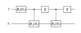
Figure 2: The quantum circuit for the dependency relationship of $y\rightarrow x_{1}$.

Take the naïve Bayesian network in Fig. 1a as an example. These are one label node $y$ and one feature node $x_{1}$, and each node has only 2 values, either 0 or 1. By statistically counting the class-prior probabilities $P(y=0)$ and the class-conditional probabilities $P(x_{1}|y=0)$ and $P(x_{1}|y=1)$, one can construct a quantum circuit as depicted in Fig. 2. In this case, the output of the circuit is

$$\sum_{i,j=\{0,1\}}\sqrt{P(y=i)}\sqrt{P(x_{1}=j|y=i)}\ket{ij}.$$ (15)

Note that the probabilities of different label values and feature values are encoded in the amplitude of the output state, which is the same as Eq. (7). That is, the quantum circuit implements the naïve QBC. By continuously adding new feature nodes to the quantum circuit and establishing controlled rotations between parent nodes and child nodes, one can construct QBCs based on different dependency relationships. Another example is a Bayesian network with multiple features. That is, the naïve QBC with $n=3$ features is shown in Fig. 3a.

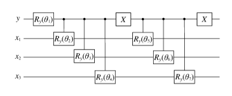
(a) The naïve QBC with 3 features.

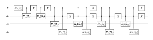
(b) The SN-QBC based on SPODE structure with 3 features and $x_{1}$ as the superparent node.

Figure 3: Quantum circuits of QBCs.

In the prediction stage, for a given feature value $X=X^{\ast}$, one only needs to obtain the probabilities of the basis state $\ket{y=i,X=X^{\ast}}$ by measurement. That is, obtain the values of $P(y=0,X=X^{\ast})$ and $P(y=1,X=X^{\ast})$, and choose the $y$ value associated with the higher probability as the classification outcome of the QBC.

III.2 SPODE-QBC

The construction method of SN-QBC based on the SPODE structure is as follows. There are $n$ feature nodes $x_{1}$, $x_{2}$, $\cdots$, $x_{n}$. Without loss of generality, assume that $x_{1}$ is the superparent feature as shown in Fig. 1b. The quantum circuit of SN-QBC consists of $n+1$ qubits, corresponding to the label node $y$ and $n$ feature nodes $x_{1}$ to $x_{n}$, and all nodes are initialized to $\ket{0}$. Firstly, for the label node $y$, the class-prior probability $P(y=0)$ is counted and encoded by $R_{y}(\cdot)$, where the rotation angle is set as $\theta_{1}=f(P(y=0))$. Secondly, for the superparent $x_{1}$, one needs to count the class-conditional probabilities $P(x_{1}|y=0)$ and $P(x_{1}|y=1)$ and encode these probabilities by using $X$ and $CR_{y}(\cdot)$, with the controlled rotation angles being set as $\theta_{2}=f(P(x_{1}|y=0))$ and $\theta_{3}=f(P(x_{1}|y=1))$, respectively. For the remaining feature nodes $x_{2}$ to $x_{n}$, since each node has two parent nodes, four $C^{2}R_{y}(\cdot)$ are used to encode the corresponding class-conditional probabilities $P(x_{j}|y,x_{1})$, where the controlled rotation angles are set as $f(P(x_{j}|y,x_{1}))$ given the values of $y$ and $x_{1}$. That is, when the control bits are $yx_{1}=00,01,10,11$, the corresponding controlled rotation angles are set as $f(P(x_{j}=0|y=0,x_{1}=0))$, $f(P(x_{j}=0|y=0,x_{1}=1))$, $f(P(x_{j}=0|y=1,x_{1}=0))$, and $f(P(x_{j}=0|y=1,x_{1}=1))$, respectively.

For example, for a SPODE structured Bayesian network with 3 features shown in Fig. 1b, the quantum circuit of the SN-QBC can be seen in Fig. 3b. The output of the SPODE circuit is

$$\sum_{i,j,k,l=\{0,1\}}\sqrt{P(y=i)P(x_{1}=j|y=i)P(x_{2}=k|y=i,x_{1}=j)P(x_{3}=l|y=i,x_{1}=j)}\ket{ijkl}.$$ (16)

III.3 TAN-QBC

For a SN-QBC based on the TAN structure, one needs to obtain the TAN structure Bayesian network firstly. The TAN structure Bayes classifier is generated based on the maximum-weighted spanning tree algorithm Camerini-452 ; Zhou-423 , which includes the following steps Zhou-423 .

1. Calculate the conditional mutual information between any two nodes $x_{i}$ and $x_{i}$ using the following equation

   $$I(x_{i},x_{j}|y):=\sum_{x_{i},x_{j},c\in Y}P(x_{i},x_{j}|c)\log\frac{P(x_{i},x_{j}|c)}{P(x_{i}|c)P(x_{j}|c)}.$$ (17)

2. Build a complete graph among nodes and set $I(x_{i},x_{j}|y)$ as the weight between $x_{i}$ and $x_{j}$.

3. Construct the maximum-weighted spanning tree of the complete graph and set the direction of each edge outward from the root.

4. Add the label node $y$ and directed edges from $y$ to each node.

For a Bayesian network with a TAN structure, the quantum circuit of the corresponding SN-QBC can be constructed as follows. The label node $y$ and each feature node are initialized to $\ket{0}$. Firstly, the class-prior probability $P(y=0)$ is encoded by $R_{y}(f(P(y=0)))$. Then, starting from the root node of the feature spanning tree, the class-conditional probabilities of each node are encoded layer by layer. For feature $x_{j}$, its conditional probabilities $P(x_{j}|y,x_{\text{parent}_{1}},\cdots,x_{\text{parent}_{n_{j}}})$ are encoded as the rotation angles of $C^{n}R_{y}$ gates, where $x_{\text{parent}_{1}}$, $\cdots$, $x_{\text{parent}_{n_{j}}}$ are $n_{j}$ parent nodes of $x_{j}$ on the upper layer.

Fig. 4a gives a simple example of a Bayesian network with a TAN structure. One can construct the corresponding QBC based on the given Bayesian network. The circuit of the SN-QBC based on the TAN structure in Fig. 4a is presented in Fig. 4b. The rotation angles of the label node $y$ and the root node $x_{1}$ of the spanning tree are set as the naïive QBCs shown in Sect. III.1. The rotation angles of $C^{2}R_{y}$ gates acting on $x_{3}$ are set as $f(P(x_{3}=0|yx_{1}=00))$, $f(P(x_{3}=0|yx_{1}=01))$, $f(P(x_{3}=0|yx_{1}=10))$, and $f(P(x_{3}=0|yx_{1}=11))$, respectively. While the rotation angles of $C^{2}R_{y}$ gates acting on $x_{2}$ are set as $f(P(x_{2}=0|yx_{3}=00))$, $f(P(x_{2}=0|yx_{3}=01))$, $f(P(x_{2}=0|yx_{3}=10))$, and $f(P(x_{2}=0|yx_{3}=11))$, respectively. The output of the TAN structure SN-QBC is

$$\sum_{i,j,k,l=\{0,1\}}\sqrt{P(y=i)P(x_{1}=j|y=i)P(x_{3}=k|y=i,x_{1}=j)P(x_{2}=l|y=i,x_{3}=k)}\ket{ijkl}.$$ (18)

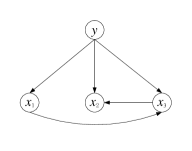
(a) The TAN structure Bayesian network.

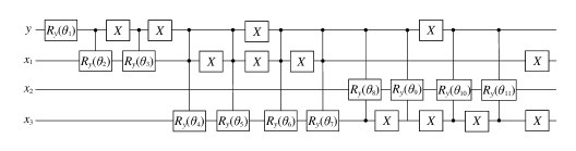
(b) The circuit of the SN-QBC based on the TAN structure.

Figure 4: The quantum circuit of the SN-QBC with TAN structure.

III.4 SN-QBC Based on the Symmetric Relationship of Image Features

Both the naïve Bayes classifier and the semi-naïve Bayes classifier only consider the dependencies between a small number of feature nodes. Note that there are symmetric relationships among the sampled features in some images, such as the digits “6” and “9” shown in Fig. 5, where there exist symmetric relationships between features $x_{2}$ and $x_{5}$, and $x_{3}$ and $x_{4}$. These symmetric relationships of image features can be used to build Bayesian networks, which can then be used to establish corresponding SN-QBCs. The method for constructing a Bayesian network based on the symmetric relationships of image features is as follows.

1. Establish a naïve Bayesian network as shown in Fig. 1a;

2. Consider the symmetric relationship of features in the sample images and add a directed edge between each pair of features that are symmetrical to each other.

For example, for an image dataset of digits “6” and “9”, a Bayesian network can be established as shown in Fig. 5.

For the Bayesian network with symmetric relationships between features, in the case of not considering the label node $y$, the network will consist of several independent trees. In this case, one can construct the corresponding QBC by using the method for the QBC based on the TAN structure in Sect. III.3. That is, each node is initialized to $\ket{0}$ and the class-prior probability $P(y=0)$ is encoded firstly. After that, each independent tree is considered separately. For each tree, starting from the root node, the class-conditional probabilities of each node are encoded layer by layer, respectively.

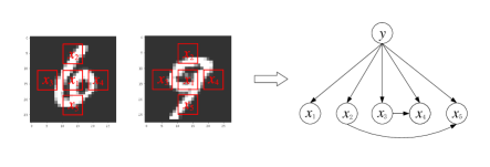
Figure 5: The Bayesian network based on symmetric relationships of features.

IV Image Classification Based on QBCs

The key to the accuracy of a Bayesian classifier lies in feature selection and the structure of Bayesian networks. In this paper, we propose an image classification framework based on QBCs and local feature sampling, as illustrated in Fig. (6). Firstly, some local areas are selected in an image for feature sampling. Then, the sampled pixels are pooled and binarized to obtain local binary features. Finally, a QBC can be constructed based on a Bayesian network model with local features as nodes for image classification.

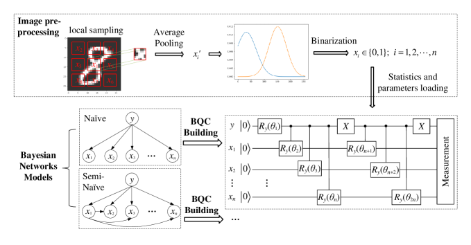
Figure 6: The framework of image classifications based on QBCs.

IV.1 Local Features Sampling

For image classifications using a naïve QBC, if each pixel of the image is taken as a node of a Bayesian network, the network will be very complex. For example, a 28*28 image requires 784 nodes to represent the network. Although $n$ qubits can form a feature space with a dimension of $2^{n}$, the resources required for the quantum Bayesian networks are still relatively large. In addition, considering the complex relationship of interdependence among features, the complexity of Bayesian networks will continue to increase, which hinders the implementation of QBCs on current NISQ devices.

To reduce computational complexity and effectively utilize image features for classification, we propose the local feature sampling method. This method aims to obtain a small number of local key features from images. For image classification, background pixels shared by some images might not provide useful information for accurate classification by Bayes classifiers. The local feature sampling method can reduce the number of feature nodes in Bayesian networks, decrease the scale and computational complexity of QBCs, and diminish the influence of quantum noise, which is beneficial for the experimental implementation of quantum circuits.

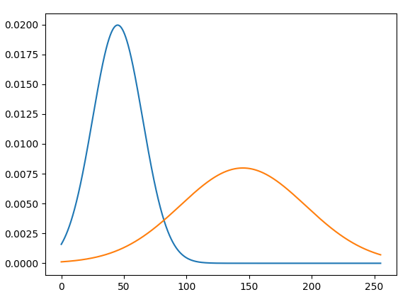
(a) One intersection.

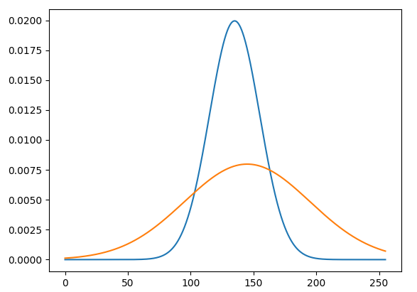
(b) Two intersections.

Figure 7: Two Gaussian functions with intersections.

As for data preprocessing, the local feature sampling method is illustrated in Fig. 6, which is performed as follows.

1. Local sampling and average pooling. Using a convolution operation on the sampling block and the convolution kernel, an image is locally sampled according to the specified block size (convolution kernel size). Next, the appropriate average pooling value $x^{\prime}_{i}$ of the feature node $x_{i}$ in the Bayesian network is obtained by applying average pooling YuWang-424 .

2. Feature binarization. In a classical Bayes classifier, assume that $P(x_{i}|c)\sim N(\mu_{c,i},\sigma_{c,i}^{2})$, where $\mu_{c,i}$ and $\sigma_{c,i}^{2}$ are the mean and the variance of the feature $x_{i}$ on the $c$-th class. One can obtain the class-prior probability by calculating the probability density function. However, it is challenging to replicate this process for a QBC. In this case, binarization is used to transform $x_{i}$ into 0 or 1 such that a single qubit can represent it.

   Here, we use the maximum likelihood estimation (MLE) Dutilleul-453 ; BoullE-425 method adopted in classical Bayes classifiers for obtaining class-conditional probabilities of continuous variables. For the binary classification case, this method runs as follows.

   Assume that $P(x_{i}|c_{0})\sim N(\mu_{c_{0},i},\sigma_{c_{0},i}^{2})$ and $P(x_{i}|c_{1})\sim N(\mu_{c_{1},i},\sigma_{c_{1},i}^{2})$. When two Gaussian functions have only one intersection, which is denoted as $x_{\text{ins}}$, as shown in Fig. (7a), the feature value is set as follows.

   $$x_{i}=\begin{cases}0,&\text{if}\ x^{\prime}_{i}\leq x_{\text{ins}}\ \text{and}\ \mu_{c_{0},i}\leq\mu_{c_{1},i},\ \text{or}\ x^{\prime}_{i}>x_{\text{ins}}\ \text{and}\ \mu_{c_{0},i}>\mu_{c_{1},i};\\ 1,&\text{otherwise.}\end{cases}$$ (19)

   where $x^{\prime}_{i}$ is the average pooling value generated by the the average pooling processing. If there are two intersection points $x_{\text{ins1}}$ and $x_{\text{ins2}}$ with $x_{\text{ins1}}\leq x_{\text{ins2}}$, as shown in Fig. (7b), in the cases where $\mu_{c_{0},i}\leq\mu_{c_{1},i}$, the feature value is set as

   $$x_{i}=\begin{cases}0,&\text{if}\ x^{\prime}_{i}\leq x_{\text{ins1}},\ \text{or}\ x_{\text{ins1}}\leq x^{\prime}_{i}\leq x_{\text{ins2}}\ \text{and}\ |x_{\text{ins1}}-x^{\prime}_{i}|\leq|x_{\text{ins2}}-x^{\prime}_{i}|;\\ 1,&\text{otherwise.}\end{cases}$$ (20)

   Conversely, when $\mu_{c_{0},i}>\mu_{c_{1},i}$, the feature value is set as

   $$x_{i}=\begin{cases}1,&\text{if}\ x^{\prime}_{i}\leq x_{\text{ins1}},\ \text{or}\ x_{\text{ins1}}\leq x^{\prime}_{i}\leq x_{\text{ins2}}\ \text{and}\ |x_{\text{ins1}}-x^{\prime}_{i}|\leq|x_{\text{ins2}}-x^{\prime}_{i}|;\\ 0,&\text{otherwise.}\end{cases}$$ (21)

By utilizing the aforementioned method, it is possible to obtain a limited number of local features. These local features serve as nodes of Bayesian networks and are utilized to construct QBCs.

IV.2 Image Classification Algorithm Based on Quantum Bayes Classifier

The image classification algorithm based on QBCs and local feature sampling is shown in Fig. (6). The algorithm consists of two stages, namely the image preprocessing stage, and the Bayesian networks and QBCs construction stage. In the image preprocessing stage, certain local areas are chosen for sampling. After that, the sampled features are pooled, and the Gaussian method is used for binarization. This process converts the sampled key features into either 0 or 1, allowing a feature to be represented by a single qubit in QBCs. In the second stage, a Bayesian network model is selected and the corresponding QBC is constructed with local key features as nodes. The algorithm runs as follows.

1. A Bayesian network is selected.

2. Local sampling and average pooling are performed on sample images, and the mean value $\mu_{i}$ and variance $\sigma_{i}$ of the corresponding features are calculated. The Gaussian binarization method is executed to obtain the binarized features, as described in Sect. IV.1.

3. The QBC circuit is constructed based on the chosen Bayesian network model by using local binarized features as nodes. Also see Sect. III.

4. The class prior probability and class conditional probability required for the Bayesian network are calculated statistically. These values are then loaded into the QBC circuit as controlled angles to complete the construction of the QBC.

5. To predict the class of a new image, one needs to repeat the step 2 to obtain a new local key feature $X^{\prime}$, and then measure the probabilities of states $\ket{0X^{\prime}}$ and $\ket{1X^{\prime}}$ on the QBC circuit. The class with the highest probability will be the classification result of the image.

V Simulations

In this paper, we test our QBCs using the MNIST LecunBottou-417 and Fashion-MNIST XiaoRasul-416 datasets. The MindQuantum Mindquantum-418 quantum simulation platform is used as the implementation platform for simulation of QBCs. The sampling block size is set to 7*7, and the average pooling method is applied. All images are sampled according to the sampling positions shown in Fig. (8) to obtain 9 local key features ($n=9$).

As is shown in Fig. (8), four Bayesian network models are used to construct four corresponding QBCs, i.e., the naïve QBC, the SN-QBC based on the SPODE structure (SPODE-QBC), the SN-QBC based on the TAN structure (TAN-QBC), and the SN-QBC based on the symmetric relationships of features (symmetric-QBC). For the TAN structures of the MNIST and Fashion-MNIST datasets, the spanning trees of the training data of the two datasets are calculated according to the maximum weighted spanning tree algorithm Camerini-452 ; Zhou-423 introduced in Sect. III.3.

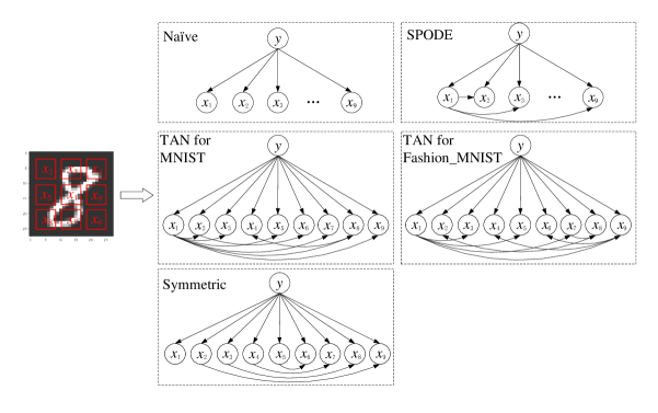
Figure 8: The sampling points and four types of Bayesian networks used in the simulation, i.e., the naïve, the SPODE, the TAN, and the symmetric Bayesian networks.

V.1 The Accuracy of Binary Classification

The MNIST and Fashion-MNIST datasets are used to verify the binary classification effects of four QBCs on every two image classes. Fig. 9 and Fig. 10 show the classification accuracies of the four QBCs in the MNIST and the Fashion-MNIST datasets, respectively.

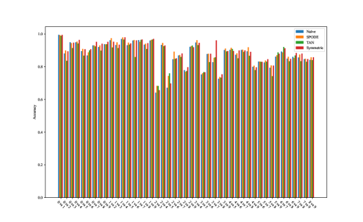
Figure 9: The classification accuracies of every two classes in the MNIST dataset on the naïve QBC, the SPODE-QBC, the TAN-QBC, and the symmetric-QBC.

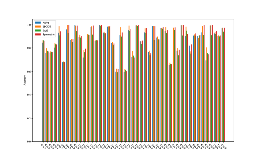
Figure 10: The classification accuracies of every two classes in the Fashion-MNIST dataset on the naïve QBC, the SPODE-QBC, the TAN-QBC, and the symmetric-QBC.

It can be seen from Fig. 9 that the symmetric-QBC shows a better classification performance in most cases. While as in shown in Fig. 10, the SPODE-QBC shows better results in the Fashion-MNIST dataset in most cases, and the symmetric-QBC also exhibits better classification results on some data.

In addition, the simulation results show that QBCs still does not achieve ideal classification results for some data in these two datasets, which lies in the following reasons.

1. The Bayesian network used in the simulation may not be suitable for all data. Different Bayesian networks should be considered for different data;

2. The hyperparameters involved in the simulation, such as the sampling block size, the convolution kernel size, and the pooling method, etc., has a significant impact on the results, which should be selected carefully;

3. Some features extracted from local sampling and binarization procedure can not distinguish data from two classes very well. Other sampling and binarization methods could be considered.

V.2 Overall Performance of QBCs

To evaluate the overall performance of each QBC, the average classification accuracy, variance, average precision, average recall, and average $F_{1}$ score Liu-408 ; Caelen-407 are calculated. The average classification accuracy of a binary classifier for two classes in the MNIST and Fashion-MNIST datasets is defined as

$$\overline{acc}=\frac{1}{45}\sum_{i=0}^{8}\sum_{j=i+1}^{9}acc_{ij},$$ (22)

where $acc_{ij}$ represents the accuracy of binary classification of classes $i$ and $j$. The variance is defined as

$$s^{2}=\frac{1}{45}\sum_{i=0}^{8}\sum_{j=i+1}^{9}(\overline{acc}-acc_{ij})^{2}.$$ (23)

While the average precision, average recall, and average $F_{1}$ score are defined as

$$\overline{prec}=\frac{1}{45}\sum_{i=0}^{8}\sum_{j=i+1}^{9}\frac{TP_{ij}}{TP_{ij}+FP_{ij}},\quad\overline{recall}=\frac{1}{45}\sum_{i=0}^{8}\sum_{j=i+1}^{9}\frac{TP_{ij}}{TP_{ij}+FN_{ij}},\quad F_{1}=\frac{2*\overline{prec}*\overline{recall}}{\overline{prec}+\overline{recall}},$$ (24)

where TP means the number of true positive, FP means false positive, and FN means false negative. Table 1 shows the overall performance of the four QBCs mentioned above for all binary classification pairs in the MNIST and Fashion-MNIST datasets. As is shown in Table 1, the SPODE-QBC and symmetric-QBC exhibit good classification accuracies in both the MNIST and Fashion-MNIST datasets, while the naïve-QBC and TAN-QBC also show relatively good classification effects. On the whole, the symmetric-QBC performs best in the MNIST dataset, while the SPODE-QBC performs best in the Fashion-MNIST dataset.

Table 1: Overall performances of the four QBCs in two datasets.

Dataset	Classifier	$\overline{acc}$	$s^{2}$	$\overline{precision}$	$\overline{recall}$	$F_{1}$
MNIST	Naïve-QBC	0.8767	0.0777	0.8844	0.8689	0.8762
	SPODE-QBC	0.8873	0.0707	0.8930	0.8808	0.8864
	TAN-QBC	0.8055	0.0888	0.7390	0.9775	0.8388
	Symmetric-QBC	0.8889	0.0739	0.8930	0.8813	0.8867
Fashion-MNIST	Naïve-QBC	0.8712	0.1128	0.8726	0.8748	0.8728
	SPODE-QBC	0.8916	0.1080	0.8863	0.9107	0.8962
	TAN-QBC	0.8739	0.1115	0.8343	0.9602	0.8894
	Symmetric-QBC	0.8834	0.1112	0.8807	0.8942	0.8859

V.3 Comparison with Other Classifiers

Table 2 shows the comparison of classification performance of the classical Gaussian naïve Bayes classifier GaussianNB , the quantum convolutional neural network (QCNN) HurKim-435 , and four QBCs for classes 0 and 1 in the MNIST and Fashion-MNIST datasets. The results show that QBCs performs better than the classical Bayes classifier and QCNN in the MNIST dataset, while the QCNN performs best in the Fashion-MNIST dataset. It is important to note that the classical Bayesian classifier and quantum neural network classifier use all 786 features, while the four QBCs in this paper use only 9 binary features. The simulation also shows that adjusting the sampling block size and the convolution kernels can improve the accuracy of QBCs, but this may not be effective for all classes of images. Specific analysis and adaptation are required for a specific task.

Table 2: Comparison of classification accuracy of classes 0 and 1 in MNIST and Fashion-MNIST by different classifiers.

Classifier	MNIST 0 vs 1	Fashion-MNIST: 0 (t-shirt) vs 1 (trouser)
Classical naïve Bayes GaussianNB	0.985	0.897
QCNN HurKim-435	0.987	0.941
Naïve-QBC	0.994	0.844
SPODE-QBC	0.992	0.866
TAN-QBC	0.968	0.820
Symmetric-QBC	0.994	0.861

VI Discussions & Conclusions

In this paper, we study the constructions of QBCs using Bayesian networks. Based on four kinds of Bayesian networks, four QBCs are implemented, that is, the naïve-QBC, the SPODE-QBC with the feature in an image center as the ’superparent’, the TAN-QBC, and the symmetric-QBC.

We apply these QBCs to image classification and propose the image classification algorithm. To reduce the computational complexity, a local feature sampling method is designed to extract a few key features from a huge number of image pixels. By keeping key features, this method maintains high classification accuracies while reducing the number of features. Adjusting the sampling block size and utilizing different convolution kernels can further improve the accuracies of QBCs.

The classification effects of QBCs are verified on the MindQuantum platform for the MNIST and Fashion-MNIST datasets, respectively. The results show that QBCs perform well for image classification. We also compare QBCs with the classical Bayesian classifier and QCNN that use all features directly, which shows that QBCs using a few features still have advantages in some cases.

Unlike QCNN classifiers HurKim-435 ; CongChoi-181 , QBCs do not require a time-consuming training process. They only require to calculate the corresponding parameters statistically and load them into quantum circuits, while the classification decision can be made by measuring quantum circuits, which is faster, lower in computational complexity, and less resource-consuming than QCNN.

At present, there does not exist a general QBC that performs well with all types of data. Building QBCs based on alternative varieties of Bayesian networks that work well with various datasets would be intriguing.

Data availability statement

The data that support the findings of this study are available from the corresponding author upon reasonable request.

References

- (1) K. Mosegaard, M. Sambridge, Monte carlo analysis of inverse problems, Inverse Probl., 2002, 18(3), R29
- (2) M. Modarres, K. Groth, Reliability and risk analysis (CRC Press, 2023)
- (3) N. Daniels, Justice, health, and healthcare, Am. J. Bioeth., 2001, 1(2), 2
- (4) P. Gary Jarrett, Logistics in the health care industry, Int. J. Phys. Distrib. Logist. Manag., 1998, 28(9/10), 741
- (5) H. Wong, W. Lin, H. Laure, Multi-polarization reconfigurable antenna for wireless biomedical system, IEEE Trans. Biomed. Circuits Syst., 2017, 11(3), 652
- (6) J. Kwisthout, Most probable explanations in bayesian networks: Complexity and tractability, Int. J. Approx. Reason., 2011, 52(9), 1452
- (7) M. Chickering, D. Heckerman, C. Meek, Large-sample learning of bayesian networks is np-hard, J. Mach. Learn. Res., 2004, 5, 1287
- (8) P.W. Shor, Polynomial-time algorithms for prime factorization and discrete logarithms on a quantum computer, SIAM J. Sci. Statist. Comput., 1997, 26(5), 1484
- (9) L.K. Grover, Quantum mechanics helps in searching for a needle in a haystack, Phys. Rev. Lett., 1997, 79(2), 325
- (10) P. Rebentrost, M. Mohseni, S. Lloyd, Quantum support vector machine for big data classification, Phys. Rev. Lett., 2014, 113(13), 130503
- (11) Y. Dang, N. Jiang, H. Hu, Z. Ji, W. Zhang, Image classification based on quantum k-nearest-neighbor algorithm, Quantum Inf. Process., 2018, 17, 1
- (12) I. Cong, S. Choi, M.D. Lukin, Quantum convolutional neural networks, Nat. Phys., 2019, 15(12), 1273
- (13) I. Kerenidis, J. Landman, A. Prakash, Quantum algorithms for deep convolutional neural networks, arXiv preprint arXiv:1911.01117, 2019
- (14) T. Hur, L. Kim, D.K. Park, Quantum convolutional neural network for classical data classification, Quantum Mach. Intell., 2022, 4(1), 3
- (15) L.H. Gong, J.J. Pei, T.F. Zhang, N.R. Zhou, Quantum convolutional neural network based on variational quantum circuits, Opt. Commun., 2024, 550, 129993
- (16) M. Schuld, F. Petruccione, Quantum ensembles of quantum classifiers, Sci. Rep., 2018, 8(1), 2772
- (17) A. Macaluso, L. Clissa, L. Stefano, C. Sartori, Quantum ensemble for classification, arXiv preprint arXiv:2007.01028, 2020
- (18) I.C. Araujo, A.J. Da Silva, Quantum ensemble of trained classifiers, in International Joint Conference on Neural Networks (IJCNN) (IEEE, Glasgow, UK, 2020), (IJCNN), pp. 1–8
- (19) A. Macaluso, S. Lodi, C. Sartori, Quantum algorithm for ensemble learning, in 21st Italian Conf. Theoretical Computer Science (CEUR-WS.org, 2020), pp. 149–154
- (20) X.Y. Zhang, M.M. Wang, An efficient combination strategy for hybrid quantum ensemble classifier, Int. J. Quantum Inf., 2023, 21(06), 2350027
- (21) S. Youssef, Quantum mechanics as an exotic probability theory, arXiv preprint quant-ph/9509004, 1995
- (22) M. Ozols, M. Roetteler, J.R.M. Roland, Quantum rejection sampling, ACM Trans. Comput. Theory, 2013, 5(3), 1
- (23) C. Moreira, A. Wichert, Quantum-like bayesian networks for modeling decision making, Front. Psychol., 2016, 7, 11
- (24) S. Woerner, D.J. Egger, Quantum risk analysis, npj Quantum Inf., 2019, 1(5), 15
- (25) S.E. Borujeni, S. Nannapaneni, N.H. Nguyen, E.C. Behrman, J.E. Steck, Quantum circuit representation of bayesian networks, Expert Syst. Appl., 2021, 176, 114768
- (26) I. Rish, Others, An empirical study of the naive bayes classifier, in IJCAI 2001 workshop on empirical methods in artificial intelligence, vol. 3, pp. 41–46
- (27) K.M. Leung, Others, Naive bayesian classifier, Polytechnic University Department of Computer Science/Finance and Risk Engineering, 2007, 123
- (28) I. Kononenko, Semi-naive bayesian classifier, in Machine Learning—EWSL-91: European Working Session on Learning (Springer, Porto, Portugal, 1991), pp. 206–219
- (29) Z.H. Zhou, Machine learning (Springer Nature, 2021)
- (30) MindQuantum Developer. Mindquantum, version 0.6.0, 2021. URL https://gitee.com/mindspore/mindquantum
- (31) Y. LeCun, L. Bottou, Y. Bengio, P. Haffner, Gradient-based learning applied to document recognition, Proc. IEEE, 1998, 86(11), 2278
- (32) H. Xiao, K. Rasul, R. Vollgraf, Fashion-mnist: a novel image dataset for benchmarking machine learning algorithms, arXiv preprint arXiv:1708.07747, 2017
- (33) J.O.R. Offmann-J O Rgensen, G. Pisier, The law of large numbers and the central limit theorem in banach spaces, Ann. Probab., 1976, pp. 587–599
- (34) P.M. Camerini, The min-max spanning tree problem and some extensions, Inf. Process. Lett., 1978, 7(1), 10
- (35) M.A. Nielsen, I.L. Chuang, Quantum Computation and Quantum Information (Cambridge University Press, Cambridge, UK, 2000)
- (36) D. Yu, H. Wang, P. Chen, Z. Wei, Mixed pooling for convolutional neural networks, in Rough Sets and Knowledge Technology: 9th International Conference, RSKT 2014 (Springer International Publishing, Shanghai, China, 2014), pp. 364–375
- (37) P. Dutilleul, The mle algorithm for the matrix normal distribution, J Stat. Comput. Simul., 1999, 64(2), 105
- (38) M. Boull E, Modl: a bayes optimal discretization method for continuous attributes, Mach. Learn., 2006, 65, 131
- (39) Y. Liu, Z. Yangming, A strategy on selecting performance metrics for classifier evaluation, Int. J. Mob. Comput., 2014, 6(4), 20
- (40) O. Caelen, A bayesian interpretation of the confusion matrix, Ann. Math. Artif. Intell., 2017, 81(3–4), 429
- (41) Gaussian naive bayes. URL https://scikit-learn.org/stable/modules/generated/sklearn.naive_bayes.GaussianNB.html