Progress report on testing robustness of the Newton method in data analysis on 2-point correlation function using a MILC HISQ ensemble

Abstract

We report recent progress in data analysis on the two point correlation functions which will be prerequisite to obtain semileptonic form factors for the $B_{(s)}\to D_{(s)}\ell\nu$ decays. We use a MILC HISQ ensemble for the measurement. We use the HISQ action for light quarks, and the Oktay-Kronfeld (OK) action for the heavy quarks ($b$ and $c$). We used a sequential Bayesian method for the data analysis. Here we test the new fitting methodology of Benjamin J. Choi in a completely independent manner.

1 Introduction

Semileptonic form factors for the $B\to D^{(*)}l\nu$ decays can probe the Cabibbo-Kobayashi-Maskawa (CKM) matrix element $\left|V_{cb}\right|$ [1]. This requires the precise data analysis on 2-point correlation functions [2]. Here, we present our recent progress in data analysis on 2-point correlation functions. This work provides an independent cross-checking of the methodology developed by Benjamin Choi in Ref. [3].

We use the MILC HISQ ensembles for the numerical study. In Table 1 (1(a)), we summarize details on the MILC lattice a12m310. For bottom and charm quarks, we use the Oktay-Kronfeld (OK) action [4]. In Table 1 (1(b)), we summarize details on hopping parameters for bottom quarks, and light quark masses.

ID	a (fm)	$M_{\pi}$(MeV)	$L^{3}\times T$
a12m310	0.1207(11)	305.3(4)	$24^{3}\times 64$

(a) Details on the MILC lattice ensemble

$\kappa_{\text{crit}}$	$\kappa_{b}$	$m_{l}$	$N_{\text{cfg}}\times N_{\text{src}}$
0.051211	0.04102	0.0509	$1053\times 3$

(b) Hopping parameters

Table 1: Parameters for the numerical study. Here, $N_{\text{cfg}}$ ($N_{\text{src}}$) represents the number of gauge configurations (the number of measurements per gauge configuration).

2 Fit Function

Spectral decomposition of 2-pt correlation functions $C(t)$ measured on the lattice is

$$C(t)= \sum_{\tau}\left<{\mathcal{O}^{\dagger}_{\tau}(x)\mathcal{O}_{\tau}(0)}\right>$$

$$= \sum_{n=0}^{\infty}(-1)^{n(t+1)}\left|\left<{n|\mathcal{O}(0)|0}\right>\right|^{2}\left(e^{-E_{n}t}+e^{-E_{n}(T-t)}\right).$$ (1)

where the heavy-light meson operator $\mathcal{O}$ is

$$\mathcal{O}_{\tau}(x) \equiv\left[\bar{\psi}(x)\Gamma\Omega(x)\right]_{\tau}\chi(x)\,,$$ (2)

$$\Gamma =\gamma_{5}\quad\text{or}\quad\gamma_{j}\,,$$ (3)

$$\Omega(x) =\gamma_{1}^{m_{1}}\gamma_{2}^{m_{2}}\gamma_{3}^{m_{3}}\gamma_{4}^{m_{4}}\,,$$ (4)

$$x_{\mu} =m_{\mu}a\quad\text{with}\quad m_{\mu}\in Z$$ (5)

with staggered quark field $\chi(x)$, and the $\psi$ is a heavy quark field in the OK action [4]. Here, $n$ is an integer index for energy eigenstates. If $n$ is even (odd), its eigenstate has even (odd) time-parity. The oscillating terms with odd time-parity come from the temporal doubler of staggered quarks [5]. The $\tau$ represents taste degrees of freedom for staggered quarks. In our notation, $\lvert 0\rangle$ represents not the vacuum state ($\lvert\Omega\rangle$) but the heavy-light meson ground state with energy $E_{0}>0$.

Then, the $n+m$ fitting function [5] is

$$f^{n+m}(t)= g^{n+m}(t)+g^{n+m}(T-t),$$ (6)

$$g^{n+m}(t)= A_{0}e^{-E_{0}t}\Big{[}1+r_{2}e^{-\Delta E_{2}t}\times\left(1+\dots\times(1+r_{(2n-2)}e^{-\Delta E_{(2n-2)}t})\cdots\right)$$

$$-(-1)^{t}r_{1}e^{-\Delta E_{1}t}\big{(}1+\dots\times(1+r_{(2m-1)}e^{-\Delta E_{(2m-1)}t})\cdots\big{)}\Big{]}$$ (7)

where $r_{i}=\displaystyle\frac{A_{i}}{A_{i-2}}$, $\Delta E_{i}=E_{i}-E_{i-2}$ for $i\geq 1$ with $E_{-1}=E_{0}$ and $A_{-1}=A_{0}$. The $n+m$ fit implies that we include the $n$ even time-parity states and $m$ odd time-parity states in the fitting function.

3 Newton method

When we do the least $\chi^{2}$ fitting, we use the Broyden-Fletcher-Goldfarb-Shanno (BFGS) algorithm [6, 7, 8, 9] to minimize $\chi^{2}$. This algorithm belongs to a category of the quasi-Newton method in an optimization problem [10]. The quasi-Newton method requires an initial guess as input to the fitting by construction.

If a initial guess is good, the quasi-Newton method finds the minimum efficiently. If the initial guess is poor (out of radius of convergence), the number of iterations increases and the chance to find the local minima instead of the global minimum grows up. Therefore, it is essential to find a good initial guess close to the true solution (the global minimum), if we want to save computing resources. For this purpose, it is best to obtain initial guess directly from the data, as long as the computing time is negligibly small compared with that of the $\chi^{2}$ minimizer. It is the multi-dimensional Newton method combined with a scanning method [3] that satisfies these conditions.

The (1-dimensional) Newton method converges quadratically with respect to the distance from the true solution. Hence, it find a root in a few iterations, if the initial guess is sufficiently close to the true solution. However, if the initial guess is sufficiently far away from the true solution, it loses its merit completely. The scanning method converges slowly, but it can narrow down a range to find roots in a few iterations. If we combine the Newton method with the scanning method, it is possible to keep only the merits, while discarding the disadvantages. In other words, the scanning method finds a narrow range to find roots in a few iterations, and then the Newton method can find a root in a few iterations within the narrow range.

Let us consider the $1+1$ fit as an example. We feed results for the $1+0$ fit as an initial guess for the $A_{0},E_{0}$ part of the $1+1$ fit parameters. In order to obtain initial guess for the remaining parameters $r_{1}$ and $\Delta E_{1}$, we use the 4-dimensional Newton method combined with the scanning method. The initial range is set to $r_{1}\in[0,1.5]$ and $\Delta E_{1}\in[0,1.0]$ for the scanning method. After a few iterations ($1\sim 2$), the scanning method finds such a narrow range for $r_{1}$ and $\Delta E_{1}$ that we may use the Newton method [3] to find an exact solution for Eqs. 8 in a few iterations ($7\sim 10$).

The Newton method uses the same time slice combination (e.g. $\{t_{1}=t_{\min},t_{2},t_{3},t_{4}\}$ for the $1+1$ fit) as the scanning method. First, we collect all the possible time slice combinations within the fit range ( $t_{\min}\leq t\leq t_{\max}$ ; e.g. $t_{\min}=12$ and $t_{\max}=26$ for the $1+1$ fit), before using the scanning and Newton methods. A possible time slice combination should satisfy the following two conditions: 1) it must contains $t_{\min}$, and 2) the number of even time slices must be equal to that of odd time slices. For each time slice combination, we run the Newton method until we consume all the time slice combinations. If the Newton method find a good solution in a few iterations ($7\sim 10$), then we keep it, and if it fails, we discard that time slice combination. The failure rate is about $70\%$ for the 1+1 fit.

The Newton method finds a solution to satisfy the $N$ equations: $q(t_{i})=0$ with $t_{i}\in\{t_{\min},t_{2},t_{3},\ldots,t_{N}\}$, with $N=2(n+m)$ for the $n+m$ fit (e.g. $N=4$ for the $1+1$ fit).

$$q(t_{i})=\frac{f(t_{i})-C(t_{i})}{C(t_{i})}=0\,.$$ (8)

Here, $C(t_{i})$ is the 2pt correlator data coming from our numerical measurements, and $f(t)$ is the fitting function in Eq. (6). The stopping condition is

$$\max_{i=1,\dots,N}\left|q(t_{i})\right|<10^{-12}\,.$$ (9)

4 Fitting results

Here we describe our sequential Bayesian fitting procedure such as 1+0 fit $\to$ 1+1 fit $\to$ 2+1 fit $\to$ 2+2 fit in detail. We also present results for the $n+m$ fit in each stage of the sequential Bayesian method (SBM). We also explain how to perform stability tests at each stage of the SBM.

4.1 1+0 Fit

Here the fitting function is $f(t)=f^{1+0}(t)$ in Eq. (6). First we do the $\chi^{2}$ fit for the $1+0$ fit over the whole appropriate fit ranges. To find initial guess for $\chi^{2}$ minimizer, we solve the following linear equation:

$$\begin{bmatrix}\sum\limits_{i}\dfrac{C^{2}(t_{i})}{\sigma^{2}(t_{i})}&\sum\limits_{i}t_{i}\dfrac{C^{2}(t_{i})}{\sigma^{2}(t_{i})}\\ \sum\limits_{i}t_{i}\dfrac{C^{2}(t_{i})}{\sigma^{2}(t_{i})}&\sum\limits_{i}t_{i}^{2}\dfrac{C^{2}(t_{i})}{\sigma^{2}(t_{i})}\end{bmatrix}\begin{bmatrix}\ln A_{0}^{\text{ig}}\\ -E_{0}^{\text{ig}}\end{bmatrix}=\begin{bmatrix}\sum\limits_{i}\dfrac{C^{2}(t_{i})}{\sigma^{2}(t_{i})}\ln|C(t_{i})|\\ \sum\limits_{i}t_{i}\dfrac{C^{2}(t_{i})}{\sigma^{2}(t_{i})}\ln|C(t_{i})|\end{bmatrix},$$ (10)

which assumes the diagonal approximation in the covariance matrix [11]. Here $A_{0}^{\text{ig}}$, $E_{0}^{\text{ig}}$ denote the initial guesses, and $\sigma(t_{i})=\sqrt{V(t_{i},t_{i})}$, where $V(t_{i},t_{i})$ is the covariance matrix of the data $C(t_{i})$. Here the summation $\sum\limits_{i}$ is over the fit range: $t_{\min}\leq t_{i}\leq t_{\max}$. The optimal fit range for the 1+1 fit is determined by the minimum of $\chi^{2}/\text{dof}$. In Fig. 1 we present results for $\chi^{2}/\text{dof}$ as a function of $t_{\min}$ and $t_{\max}$. We find that the optimal fit range is $19\leq t\leq 28$: $t_{\min}=19$ and $t_{\max}=28$.

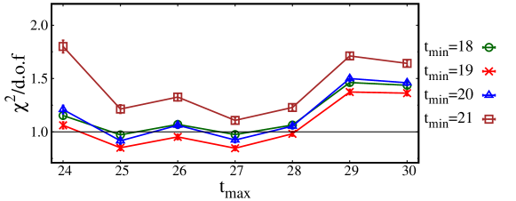
Figure 1: $\chi^{2}/\text{d.o.f}$ of the $1+0$ fit as a function of $t_{\min}$ and $t_{\max}$

Note that $t_{\max}=28$ is fixed for the remaining fits of the SBM.

Let us define the Newton mass $m^{d}_{\text{newt}}(t)=E_{0}(t)$ at zero momentum projection. At each time slice $t$, we obtain $m^{d}_{\text{newt}}(t)$ by solving two equations: $q(t)=q(t+d)=0$, using the 2-dimensional Newton method. We use the least $\chi^{2}$ fitting results for $A_{0}$ and $E_{0}$ as initial guess for the 2-d. Newton method. In Fig. (2(a)), we present results for $m^{d}_{\text{newt}}(t)$ with $d=1$ and $d=2$ as a function of time $t$.

(a) The newton mass plot

(b) Residual plot of $1+0$ fit

Figure 2: Results of $1+0$ fit

Results for the 1+0 fit are summarized in Table (2). In order to check the quality of fitting, we plot the residual, $r(t)=\dfrac{C(t)-f(t)}{\lvert C(t)\rvert}$ in Fig. 2 (2(b)). Here the red (blue) symbols represent the residual within (out of) the fit range.

Fit range	$A_{0}$	$E_{0}$	$\chi^{2}/d.o.f.$	$p$-value
[19, 28]	0.01735(125)	2.0162(38)	0.981(22)	0.448(17)

Table 2: Result of the $1+0$ fit

4.2 1+1 Fit

We use results of the 1+0 fit to determine Bayesian priors for the 1+1 fit. We set the Bayesian prior widths (BPW) to the maximum fluctuation ($\sigma_{p}^{mf}$) or the signal cut ($\sigma_{p}^{sc}$) of the $A_{0}$ and $E_{0}$ parameters. We choose $\min(\sigma_{p}^{mf},\sigma_{p}^{sc})$ for the BPW.

Starting from $t_{\min}^{1+1}=t_{\min}^{1+0}-2$, we run $t_{\min}^{1+1}$ over the lower values until $\chi^{2}/\text{dof}$ overflows the appropriate criterion.

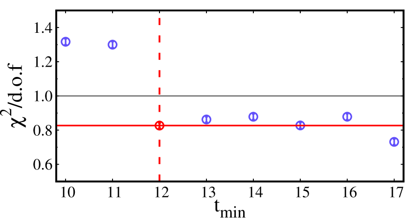
(a) Result of $\chi^{2}/\text{d.o.f}$ of $1+1$ fit

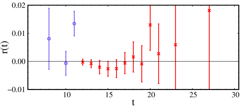
(b) Residual plot of $1+1$ fit

Figure 3: Results of $1+1$ fit

In Fig. 3 (3(a)) we present $\chi^{2}/\text{dof}$ as a function of $t_{\min}^{1+1}$. Here we find that the optimal fit range is $t_{\min}^{1+1}=12$. In Fig. 3 (3(b)) we present the residual $r(t)$ with the fit range $12\leq t\leq 28$. The 1+1 fit results are summarized in Table 3.

$t_{\min}$	$A_{0}$ $(10^{-2})$	$E_{0}$	$r_{1}$	$\Delta E_{1}$	$\frac{\chi^{2}}{\text{d.o.f.}}$
prior	1.735(1735)	2.0162(538)
12	1.847(31)	2.0198(13)	0.28(14)	0.193(39)	0.827(15)

Table 3: Result of the $1+1$ fit

4.3 2+1 Fit

First, we use the results of $1+1$ to set the BPW for $2+1$ fit. Starting from $t_{\min}^{2+1}=t_{\min}^{1+1}-2$, we run $t_{\min}^{2+1}$ over the lower values until $\chi^{2}/\text{dof}$ overflows the criterion. In Fig. 4 (4(a)) we present $\chi^{2}/\text{dof}$ as a function of $t_{\min}^{2+1}$. Here we find that $t_{\min}^{2+1}=6$ is the optimal fit range for the 2+1 fit. In Fig. 4 (4(b)) we present the residual $r(t)$ with the fit range $6\leq t\leq 28$.

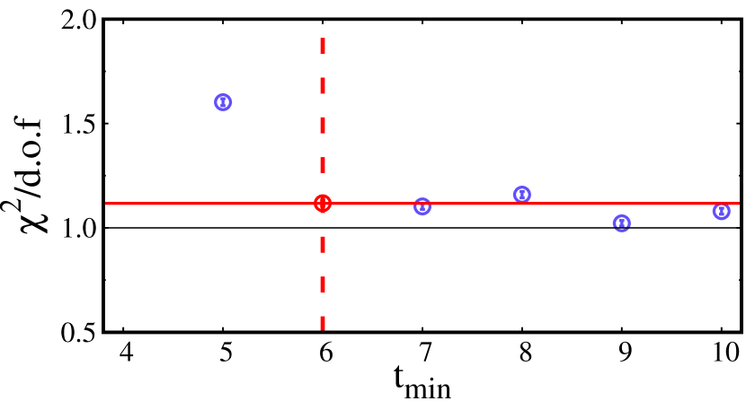
(a) Result of $\chi^{2}/\text{d.o.f}$ of $2+1$ fit

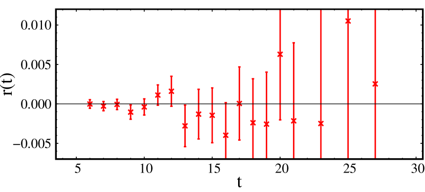
(b) Residual plot of $2+1$ fit

Figure 4: Results of $2+1$ fit

Once we choose the fit range, we can perform the stability tests to find the optimal prior widths for $A_{0}$ and $E_{0}$, which minimize prior widths with no change in fit results. Here we adopt the same notation and convention as in Ref. [12]. First, we first do the fit with maximum prior widths: $\sigma_{\text{p}}^{\max}(A_{0})=\sigma_{p}^{\text{sc}}$, and $\sigma_{\text{p}}^{\max}(E_{0})=\sigma_{p}^{\text{mf}}$, which correspond to the blue circles in Fig. 5. Here note that $\sigma^{A_{0}}_{\max}=\sigma(A_{0};\sigma_{p}^{\max}(A_{0}),\sigma_{p}^{\max}(E_{0}))$ and $\sigma^{E_{0}}_{\max}=\sigma(E_{0};\sigma_{p}^{\max}(A_{0}),\sigma_{p}^{\max}(E_{0}))$. The units for $x-$axis are $[\sigma^{A_{0}}_{\max}]=5.54\times 10^{-4}$, and $[\sigma^{E_{0}}_{\max}]=2.01\times 10^{-3}$. We find the optimal prior widths (the red square symbols, $\sigma_{p}^{\text{opt}}(A_{0}\text{ or }E_{0})$) such that they are the minimum prior widths which does not disturb the fit results obtained with the maximum prior widths. Here the $\sigma_{\sigma}$ (blue dashed lines) represents the error of the error.

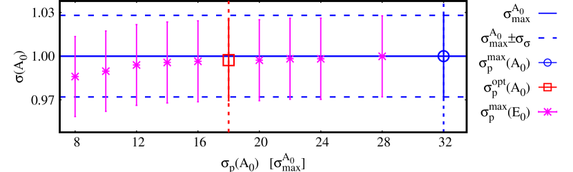
(a) Stability test on $A_{0}$.

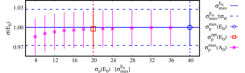
(b) Stability test on $E_{0}$.

Figure 5: Results of the stability test for the $2+1$ fit.

Results of the 2+1 fit are summarized in Table 4.

$t_{\min}$	$A_{0}$ $(10^{-2})$	$E_{0}$	$r_{1}$	$\Delta E_{1}$	$r_{2}$	$\Delta E_{2}$	$\frac{\chi^{2}}{\text{d.o.f.}}$
prior	1.789(997)	2.0180(400)	0.69(69)	0.257(257)
6	1.789(55)	2.0180(20)	0.69(3)	0.257(6)	1.04(20)	0.372(60)	1.011(14)

Table 4: Result of the $2+1$ fit

4.4 2+2 Fit

For the 2+2 fit we set the prior widths as follows.

1. [$A_{0}$ and $E_{0}$] We use the results of the stability tests for the 2+1 fit as the prior widths for $A_{0}$ and $E_{0}$.

2. [$R_{1}$ and $\Delta E_{1}$] We set the prior widths to the signal cuts for both.

3. [$R_{2}$ and $\Delta E_{2}$] We set the prior widths to the signal cuts for both.

4. [$R_{3}$ and $\Delta E_{3}$] No prior information.

Starting from $t_{\min}^{2+2}=t_{\min}^{2+1}-2=4$, we run $t_{\min}^{2+2}$ over the lower values. In Fig. 6 (6(a)) we present $\chi^{2}/\text{dof}$ as a function of $t_{\min}^{2+2}$. The physical positivity [13] constrains $t_{\min}$ such that $t_{\min}\geq 3$. Here we find that $t_{\min}^{2+2}=3$ is the optimal fit range. In Fig. 6 (6(c)) we present the residual $r(t)$ with the fit range $3\leq t\leq 28$.

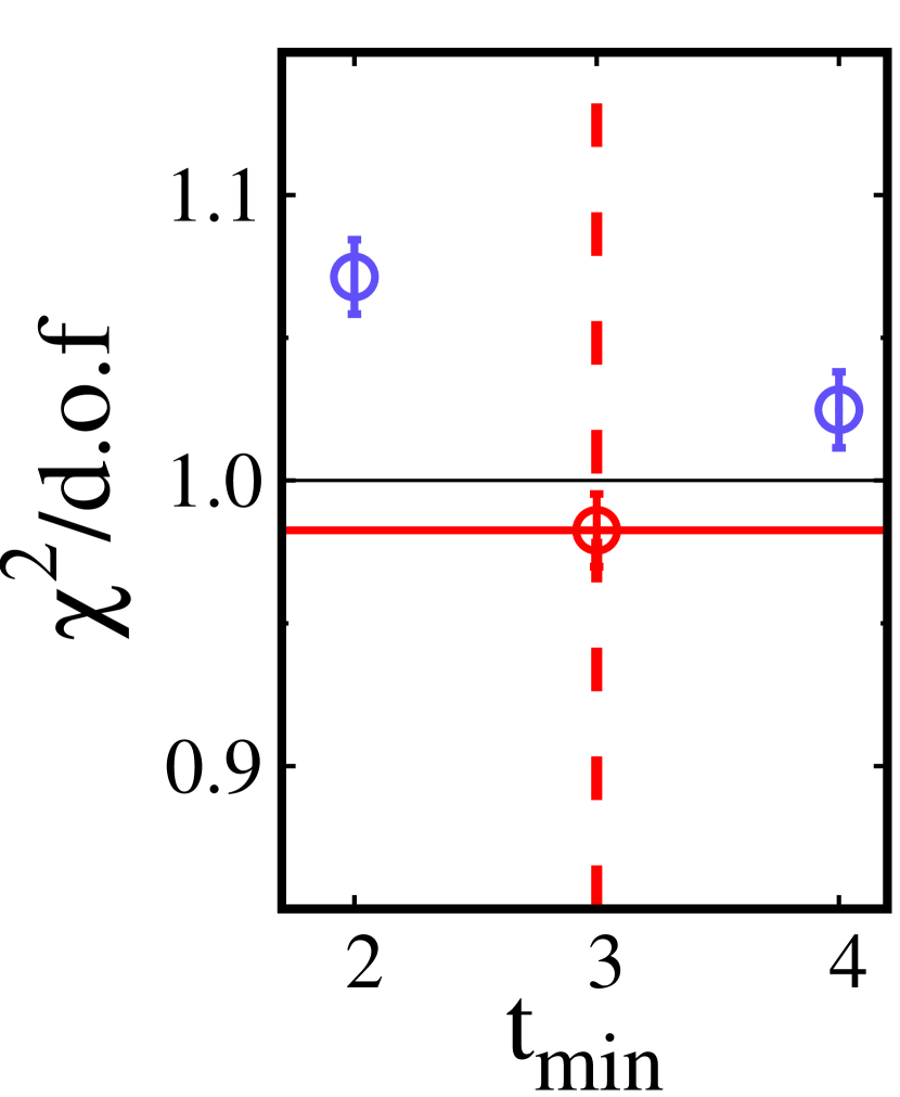
(a) $\chi^{2}/\text{d.o.f}$ of $2+2$ fit

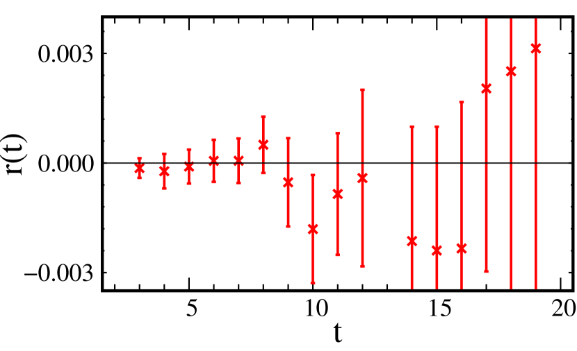
(b) Residual plot of $2+2$ fit (Zoom-in)

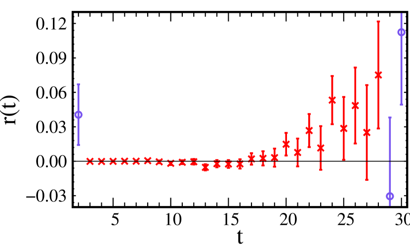
(c) Residual plot of $2+2$ fit

Figure 6: Results of $2+2$ fit

Once we choose the fit range, we do the stability tests to find the optimal prior widths for $r_{1}$ and $\Delta E_{1}$. First, we first do the fit with maximum prior widths: $\sigma_{\text{p}}^{\max}(r_{1})$, and $\sigma_{\text{p}}^{\max}(\Delta E_{1})$, which correspond to the blue circles in Fig. 7. Here note that $\sigma^{r_{1}}_{\max}=\sigma(r_{1};\sigma_{p}^{\max}(r_{1}),\sigma_{p}^{\max}(\Delta E_{1}))$ and $\sigma^{\Delta E_{1}}_{\max}=\sigma(\Delta E_{1};\sigma_{p}^{\max}(r_{1}),\sigma_{p}^{\max}(\Delta E_{1}))$, while $\sigma_{p}^{\max}(r_{1})=\sigma_{p}^{\text{sc}}(r_{1})$ and $\sigma_{p}^{\max}(\Delta E_{1})=\sigma_{p}^{\text{sc}}(\Delta E_{1})$. The units for $x-$axis are $[\sigma^{r_{1}}_{\max}]=7.8\times 10^{-2}$, and $[\sigma^{\Delta E_{1}}_{\max}]=1.31\times 10^{-2}$. In Fig. 7 the red square symbols represent the optimal prior widths, $\sigma_{p}^{\text{opt}}(r_{1}\text{ or }\Delta E_{1})$).

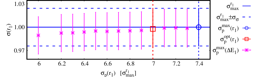
(a) Stability test on $r_{1}$.

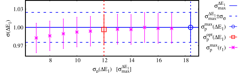
(b) Stability test on $\Delta E_{1}$.

Figure 7: Results for the stability test in the $2+2$ fit.

Results of the 2+2 fit are summarized in Table 5.

$t_{\min}$	$A_{0}$ $(10^{-2})$	$E_{0}$	$r_{1}$	$\Delta E_{1}$
prior	1.858(997)	2.0203(400)	0.58(53)	0.242(171)
3	1.858(24)	2.0203(11)	0.58(8)	0.242(13)
	$r_{2}$	$\Delta E_{2}$	$r_{3}$	$\Delta E_{3}$	$\frac{\chi^{2}}{\text{d.o.f.}}$
prior	1.91(191)	0.512(512)
3	1.91(6)	0.512(17)	1.63(19)	0.480(114)	0.983(13)

Table 5: Result of the $2+2$ fit.

References

- [1] HFLAV Collaboration, Y. Amhis et al., Averages of -hadron, -hadron, and -lepton properties as of 2021, 2206.07501.
- [2] Fermilab Lattice, MILC Collaboration, J. A. Bailey et al., Update of from the form factor at zero recoil with three-flavor lattice QCD, Phys. Rev. D 89 (2014), no. 11 114504, [1403.0635].
- [3] T. Bhattacharya, B. J. Choi, R. Gupta, Y.-C. Jang, S. Jwa, S. Lee, W. Lee, J. Leem, S. Park, and B. Yoon, Improved data analysis on two-point correlation function with sequential Bayesian method, PoS LATTICE2021 (2021) 136, [2204.05848].
- [4] M. B. Oktay and A. S. Kronfeld, New lattice action for heavy quarks, Phys. Rev. D 78 (2008) 014504, [0803.0523].
- [5] M. Wingate, J. Shigemitsu, C. T. H. Davies, G. P. Lepage, and H. D. Trottier, Heavy light mesons with staggered light quarks, Phys. Rev. D 67 (2003) 054505, [hep-lat/0211014].
- [6] C. G. BROYDEN, The Convergence of a Class of Double-rank Minimization Algorithms 1. General Considerations, IMA Journal of Applied Mathematics 6 (03, 1970) 76–90, [https://academic.oup.com/imamat/article-pdf/6/1/76/2233756/6-1-76.pdf].
- [7] R. Fletcher, A new approach to variable metric algorithms, The Computer Journal 13 (01, 1970) 317–322, [https://academic.oup.com/comjnl/article-pdf/13/3/317/988678/130317.pdf].
- [8] D. Goldfarb, A family of variable-metric methods derived by variational means, Mathematics of Computation 24 (1970) 23–26.
- [9] D. F. Shanno, Conditioning of quasi-newton methods for function minimization, Mathematics of computation 24 (1970), no. 111 647–656.
- [10] R. Fletcher, Newton-Like Methods, ch. 3, pp. 44–79. John Wiley & Sons, Ltd, 2000. https://onlinelibrary.wiley.com/doi/pdf/10.1002/9781118723203.ch3.
- [11] C. Michael, Fitting correlated data, Phys. Rev. D 49 (Mar, 1994) 2616–2619.
- [12] T. Bhattacharya, B. J. Choi, R. Gupta, Y.-C. Jang, S. Jwa, S. Lee, W. Lee, J. Leem, and S. Park, Current progress on the semileptonic form factors for decay using the Oktay-Kronfeld action, PoS LATTICE2023 (2023).
- [13] M. Luscher and P. Weisz, Definition and General Properties of the Transfer Matrix in Continuum Limit Improved Lattice Gauge Theories, Nucl. Phys. B 240 (1984) 349–361.