Testing a new general diffractive formula with gravitational wave source lensed by its companion in binary systems

Abstract

For long wavelength gravitational wave (GW), it is easy to diffract when it is lensed by celestial objects. Traditional diffractive integral formula has ignored large angle diffraction, which is adopted in most of cases. However, in some special cases (e. g. a GW source lensed by its companion in a binary system, where the lens is very close to the source), large angle diffraction could be important. Our previous works have proposed a new general diffractive integral formula which has including large angle diffraction case. In this paper, we have investigated how much difference between this general diffractive formula and traditional diffractive integral formula could be under these special cases with different parameters. We find that the module of amplification factor for general diffractive formula could become smaller than that of traditional diffractive integral basically with a factor $r_{F}\simeq 0.674$ when the distance between lens and sources is $D_{\rm LS}=1$ AU and lens mass $M_{\rm L}=1M_{\odot}$. Their difference is so significant that it is detectable. Furthermore, we find that the proportionality factor $r_{F}$ is gradually increasing from 0.5 to 1 with increasing $D_{\rm LS}$ and it is decreasing with increasing $M_{\rm L}$. As long as $D_{\rm LS}\lesssim 3$ AU (with $M_{\rm L}=1M_{\odot}$) or $M_{\rm L}\gtrsim 0.1M_{\odot}$ (with $D_{\rm LS}=1$ AU ), the difference between new and traditional formulas is enough significant to be detectable. It is promising to test this new general diffractive formula by next-generation GW detectors in the future GW detection.

1 Introduction

Gravitational lensing (GL) [1, 2] and gravitational wave (GW) [3, 4] are two important prediction of general relativity (GR). They both have been detected [5, 1, 2] and GR has been verified to right [6, 7]. Similar to GL of electromagnetic (EM) wave, there should exist GL of GW as predicted by GR. However, no strongly lensed GW event has yet confirmed up to now [8]. Current observations have searched for some lensed GW event candidates [8, 9] and it is still difficult to confirm them. With more and more GW events detected, the GL of GW events could be detected in the near future.

The detection of GL of GW has many applications. It can be used to measuring the propagation speed of GW [10, 11], constraining cosmological model [12], constraining the origin of stellar binary black hole (BH)[13], probing the nature of dark matter [14, 15, 16, 17, 18, 19, 20, 21] even the internal structure of sun [22, 23].

Different from the GL of EM wave, the wavelength of GW that we can detect could be very long, which could be close to even longer than the scale of celestial objects. Thus it is easier to take place diffraction for lensed GW. Assuming point mass lens model, diffraction effect play a critical role if lens mass is less than $10^{5}M_{\odot}\left(\frac{f}{\rm Hz}\right)^{-1}$for GW [24]. Traditional diffractive integral formula for GL of GW has been studied and applied in many literatures [1, 25, 24]. However, traditional diffractive integral formula has ignored large angle diffraction, which could be inaccurate in some special cases. Guo and Lu [26] have proposed a general diffractive integral formula to solve this problem. As discussed in [26], the value of this new formula is usually the same as traditional formula under most of cases. Nevertheless, in this paper, we will investigate how to test this new formula in some special cases and compare the difference between the traditional diffractive integral formula and new one, and discuss whether their difference can be detectable.

This paper is organized as follows. In Section 2, we review the theoretical framework of the new general diffractive integral formula, and discuss the accuracy of the traditional diffraction integral. Then we investigate observable differences in Section 3. Finally, some discussions on our results are summarized in Section 4 and we draw conclusions in Section 5. Throughout the paper, we adopt the geometrical unit system $G=c=1$.

2 Theoretical framework

Figure 1: The schematic diagram to demonstrate the geometrical configuration of the observer-lens-source system (the same as [26]). Here $D_{\rm L}$ ($D_{\rm S}$) represents the distance from the observer to the lens (source), and $D_{\rm LS}$ represents the distance between the lens and source; the distance between point $P$ and observer is $r$; $\boldsymbol{n}$ is the normal vector of the lens plane; $\boldsymbol{\eta}$ ($\boldsymbol{\xi}$) is the position vector of GW source on the source plane (GW on the lens plane).

For a GL system, its geometrical configuration is shown in Figure 1. Similar to [26], we adopt $D_{\rm S}$ ($D_{\rm L}$) to represent the distance between source (lens) and observer, and $D_{\rm LS}$ the distance between source and lens. The GW or EM wave emitted from a source at a position $\boldsymbol{\eta}$ in the source plane reaches point $P$ or $\boldsymbol{\xi}$ on the lens plane and is finally received by the observer on Earth. $\theta$ ($\theta^{\prime}$) represents the angle between the normal vector of lens plane and GW propagation direction at the position of observer (source).

It can be proven that the observed lensed waveform in the frequency domain $\tilde{\phi}^{L}$ propagating in a curved spacetime can be expressed as a surface integral at lens plane we usually use amplification factor to describe the lensing effect of this GL. The amplification factor is defined as the ratio of lensed waveform and unlensed waveform in the frequency domain:

$$F(w,\boldsymbol{y})=\frac{\tilde{\phi}^{L}(w,\boldsymbol{y})}{\tilde{\phi}(w,\boldsymbol{y})},$$ (2.1)

where $\omega$ represents the circular frequency of GW, $w=\frac{D_{\rm S}}{D_{\rm LS}D_{\rm L}}\xi_{0}^{2}\left(1+z_{\rm L}\right)\omega$ is a dimensionless frequency, $\boldsymbol{y}=\frac{D_{\rm L}}{\xi_{0}D_{S}}\boldsymbol{\eta}$ is dimensionless angular position of source, $\tilde{\phi}^{L}(w,\boldsymbol{y})$ and $\tilde{\phi}(w,\boldsymbol{y})$ are lensed and unlensed waveform of GW in the frequency domain, respectively and $\xi_{0}$ is a normalized constant of length, which is usually the Einstein radius of the lens.

Under the eikonal approximation, GW tensor or EM wave vector can be described as a scalar wave times constant basis. In usual cases of small angle diffraction, $\theta$, $\theta^{\prime}\simeq 0$, thus obliquity factor $\cos\theta$, $\cos\theta^{\prime}\simeq 1$. However, under general cases, e.g., large angle diffraction, $\cos\theta$, $\cos\theta^{\prime}\neq 1$, hence the obliquity factor can not be ignored. If we retain the obliquity factor in Kirchhoff diffraction integral formulas, it is easy to obtain (see details in [26])

$$F(w,\boldsymbol{y})=\frac{w}{4\pi i}\iint_{S}d^{2}xe^{iwT(\boldsymbol{x},\boldsymbol{y})}(\cos\theta+\cos\theta^{\prime})\cos\theta,$$ (2.2)

here $\cos\theta=\frac{\frac{D_{\rm L}}{\xi_{0}}}{\sqrt{\left(\frac{D_{\rm L}}{\xi_{0}}\right)^{2}+x^{2}}}$, $\cos\theta^{\prime}=\frac{\frac{D_{\rm LS}}{\xi_{0}}}{\sqrt{\left(\frac{D_{\rm LS}}{\xi_{0}}\right)^{2}+\left(\boldsymbol{x}-\frac{D_{\rm S}}{D_{\rm L}}\boldsymbol{y}\right)^{2}}}$ and dimensionless time delay

$$T(\boldsymbol{x},\boldsymbol{y})=\frac{1}{2}|\boldsymbol{x}-\boldsymbol{y}|^{2}-\psi(\boldsymbol{x})+\phi_{m}(\boldsymbol{y}),$$ (2.3)

with $\psi(\boldsymbol{x})$ representing the lens potential, $\phi_{m}(\boldsymbol{y})$ representing the arrival time in the unlensed case, $\boldsymbol{x}=\frac{\boldsymbol{\xi}}{\xi_{0}}$, $T(\boldsymbol{x},\boldsymbol{y})=\frac{D_{\rm L}D_{\rm LS}}{D_{\rm S}\xi_{0}^{2}}t_{\rm d}(\boldsymbol{\xi},\boldsymbol{\eta})$, where $t_{\rm d}$ is the realistic lensing time delay of the GL system.

What is more, this diffraction integral is not only applicable for GW or EM wave as an approximate formula, but also a scalar wave as an accurate formula.

2.1 Axial symmetric case

We adopt a polar coordinate system $(x,\theta_{x})$ to describe this integral, where $x$ is the radius of coordinate point, $\theta_{x}$ is the angle between $\boldsymbol{x}$ and $\boldsymbol{y}$, the positive direction of $\boldsymbol{y}$ is the polar axis. Thus Equation (2.2) can be rewritten as

$$F(w,\boldsymbol{y})=\frac{w}{4\pi i}\int_{0}^{\infty}xdx\int_{0}^{2\pi}d\theta_{x}\exp\left[iw\left(\frac{x^{2}}{2}+\frac{y^{2}}{2}-xy\cos\theta_{x}-\psi(\boldsymbol{x})+\phi_{\rm m}(\boldsymbol{y})\right)\right](\cos\theta+\cos\theta^{\prime})\cos\theta,$$ (2.4)

where $\cos\theta=\frac{\frac{D_{\rm L}}{\xi_{0}}}{\sqrt{\left(\frac{D_{\rm L}}{\xi_{0}}\right)^{2}+x^{2}}}$, $\cos\theta^{\prime}=\frac{\frac{D_{\rm LS}}{\xi_{0}}}{\sqrt{\left(\frac{D_{\rm LS}}{\xi_{0}}\right)^{2}+x^{2}+\frac{D^{2}_{\rm S}}{D^{2}_{\rm L}}y^{2}-2\frac{D_{\rm S}}{D_{\rm L}}xy\cos\theta_{x}}}.$

Under axial symmetric case, we can show the explicit expression of Equation (2.2) in a simpler form. If the mass distribution of lens is axial symmetric, $\psi(\boldsymbol{x})=\psi(x)$ is independent of $\theta_{x}$, thus this equation is reduced to

$$F(w,\boldsymbol{y})= \frac{w}{4\pi i}e^{iw(y^{2}/2+\phi_{m}(\boldsymbol{y}))}\int_{0}^{\infty}xdxe^{iw(x^{2}/2-\psi(x))}\cos\theta\int_{0}^{2\pi}d\theta_{x}e^{-iwxy\cos\theta_{x}}(\cos\theta+\cos\theta^{\prime}).$$ (2.5)

2.2 Traditional form under small angle approximation

If we adopt the small-angle approximation, i.e., $\cos\theta\simeq 1$, $\cos\theta^{\prime}\simeq 1$, the distance between point $P$ and observer $r=D_{\rm L}/\cos\theta\simeq D_{\rm L}$, which should be proper for most astrophysical lensing systems, the amplification factor can be reduced to

$$F(w,\boldsymbol{y})=\frac{w}{2\pi i}\iint d^{2}x\exp[iwT(\boldsymbol{x},\boldsymbol{y})].$$ (2.6)

This formula is widely used in the calculation of amplification factor in the diffractive regime (e.g., see [27, 28, 14, 29, 30]). Under the axial symmetric case, we have

$$F(w,\boldsymbol{y})=\frac{w}{i}e^{iw(y^{2}/2+\phi_{m}(\boldsymbol{y}))}\int_{0}^{\infty}xdxe^{iw(x^{2}/2-\psi(x))}J_{0}(wxy),$$ (2.7)

where $J_{0}(z)$ is zero-order Bessel function

$$J_{0}(z)=\frac{1}{\pi}\int_{0}^{\pi}e^{iz\cos\theta}d\theta.$$

2.3 Accuracy of the small angle approximation

Since $\frac{D_{\rm L}}{\xi_{0}}$ and $\frac{D_{\rm LS}}{\xi_{0}}$ are usually large numbers under most of cases, while $x$, $y$ are relatively small, $\frac{D_{\rm L}}{\xi_{0}}$, $\frac{D_{\rm LS}}{\xi_{0}}\gg x,y$, $\cos\theta$ and $\cos\theta^{\prime}$ can be expanded in the form of series and we have

$$\frac{(\cos\theta+\cos\theta^{\prime})\cos\theta}{2}\approx 1-\frac{3}{4}\left(\frac{x}{\frac{D_{\rm L}}{\xi_{0}}}\right)^{2}-\frac{1}{4}\left(\frac{\boldsymbol{x}-\frac{D_{\rm S}}{D_{\rm L}}\boldsymbol{y}}{\frac{D_{\rm LS}}{\xi_{0}}}\right)^{2}+...$$ (2.8)

If we regard Equation (2.2) as the corrected results, this expansion can also give an estimate to the relative error of the traditional Equation (2.6), which is roughly

$$\epsilon=\mathcal{O}\left(\left(\frac{x}{\frac{D_{\rm L}}{\xi_{0}}}\right)^{2}\right)+\mathcal{O}\left(\left(\frac{|\boldsymbol{x}-\frac{D_{\rm S}}{D_{\rm L}}\boldsymbol{y}|}{\frac{D_{\rm LS}}{\xi_{0}}}\right)^{2}\right).$$ (2.9)

The normalization length $\xi_{0}$ is usually taken as Einstein radius $\xi_{0}=r_{\rm E}=\sqrt{2R_{\rm S}\frac{D_{\rm LS}D_{\rm L}}{D_{\rm S}}}$, where $R_{\rm S}$ the Schwarzschild radius of the lens object. As discussed in [26], for the usual faraway lens, it is difficult to detect the tiny difference between our new diffractive formula and traditional diffractive formula. Thus we consider two special cases: the sun as the lens or the lens-source binary system.

2.3.1 Solar lens

The sun is nearest massive lens to us. Similar to [22, 23], we choose the sun as the lens. In this case, we adopt some typical parameters $D_{\rm L}=1$ AU=$1.5\times 10^{8}$ km, $D_{\rm LS}\sim D_{\rm S}\gg D_{\rm L}$, source (e.g. pulsar [23]) distance $D_{\rm S}\sim 1$ kpc=$3\times 10^{16}$ km (see pulsar catalog [31]), Schwarzschild radius $R_{\rm S}=3$ km for sun, and $\xi_{0}\simeq\sqrt{2R_{\rm S}D_{\rm L}}$. We can estimate

$$\frac{D_{\rm L}}{\xi_{0}}=\sqrt{\frac{D_{\rm L}}{2R_{\rm S}}}\sim 5000\gg 1,$$

thus the first term in Equation (2.9) is a small quantity. And

$$\frac{|\boldsymbol{x}-\frac{D_{\rm S}}{D_{\rm L}}\boldsymbol{y}|}{\frac{D_{\rm LS}}{\xi_{0}}}\simeq\frac{|\boldsymbol{x}-\frac{D_{\rm S}}{D_{\rm L}}\boldsymbol{y}|}{\sqrt{\frac{D_{\rm S}^{2}}{2R_{\rm S}D_{\rm L}}}}\simeq\frac{|\boldsymbol{x}-2\times 10^{8}\boldsymbol{y}|}{10^{12}}\ll 1$$

for usual $\boldsymbol{x},\boldsymbol{y}\sim O(1)$, thus the second term in Equation (2.9) is also a small quantity. Therefore, the traditional form Equation (2.6) for diffraction integral is applicable and accurate even for solar lens.

2.3.2 Lens-source binary system

Then we consider the second case (similar to [32]): if the lens and source form a binary system, source is eclipsed by the lens, thus $D_{\rm LS}\ll D_{\rm L}\simeq D_{\rm S}$. We need to stress that, the lens is not the binary system, but one component in a binary system, and the another one component in this system is source. This binary system could be binary neutron stars (NS), NS-BH binary system, compact object-star binary and so on. The lens could be not only a compact object, but also a star. Especially in NS-BH system, the stellar mass BH could be the lens and the rotating asymmetric NS could be the GW source. In this case, binary distance to us $D_{\rm L}\simeq D_{\rm S}\sim 1$ kpc=$3\times 10^{16}$ km, $D_{\rm LS}\ll D_{\rm L}$, distance between binary $D_{\rm LS}\sim 1$ AU=$1.5\times 10^{8}$ km, Schwarzschild radius $R_{\rm S}=3$ km for the lens (if its mass is around solar mass $M_{\rm L}\simeq 1M_{\odot}$) and normalization length $\xi_{0}\simeq\sqrt{2R_{\rm S}D_{\rm L}}$. Similarly, we can estimate

$$\frac{D_{\rm L}}{\xi_{0}}=\sqrt{\frac{D_{\rm L}}{2R_{\rm S}}}\sim 7.07\times 10^{7}\gg 1,$$

thus the first term in Equation (2.9) is also a small quantity. But the second term

$$\frac{|\boldsymbol{x}-\frac{D_{\rm S}}{D_{\rm L}}\boldsymbol{y}|}{\frac{D_{\rm LS}}{\xi_{0}}}=\frac{|\boldsymbol{x}-\frac{D_{\rm S}}{D_{\rm L}}\boldsymbol{y}|}{\sqrt{\frac{D_{\rm LS}^{2}}{2R_{\rm S}D_{\rm L}}}}\simeq\frac{|\boldsymbol{x}-\boldsymbol{y}|}{0.35}$$

could be greater than $1$ for $\boldsymbol{x},\boldsymbol{y}\sim O(1)$, thus the small angle approximation is no longer accurate in this case. It is clear that $\cos\theta\simeq 1$ is still accurate, but $\cos\theta^{\prime}\simeq 1$ is no longer accurate in this case. Hence the traditional form Equation (2.6) for diffraction integral is not applicable and accurate. To obtain more accurate results, we need to adopt new, general formula Equation (2.2) or (2.4) for diffraction integral to calculate amplification factor in the binary system consisting of lens and source.

3 Observable Difference

Since the difference between new and traditional diffractive integral formula is significant in the binary system consisting of lens and source, we discuss the observable differences between them from several different aspects as below.

3.1 $F$ as the function of frequency $w$

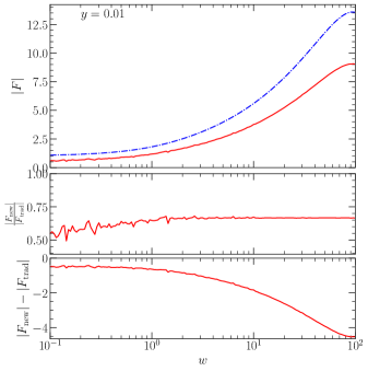
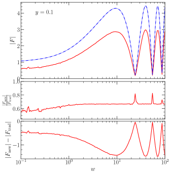
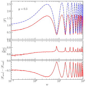
Figure 2: $|F|$ as the function of $w$ with different $y$ values, where the blue dot-dash (red solid) lines present results from traditional (new) formula in top panel of each subfigure, while other panels reflects the difference between new and traditional formula. The small-amplitude-oscillation of red curves could be due to numerical calculation error.

For simplicity, we adopt point mass lens model as our lens model, which can be used to describe BH or other compact objects. For point mass lens model, lens potential $\psi(x)=\ln x$ and it is a axial symmetric lens, thus we can adopt Equation (2.4) to calculate the new formula of diffraction integral.

As for the numerical integral, some traditional numerical integral method (e.g. [33]) are invalid for the new diffraction integral, we can adopt Levin type method [34, 35] or asymptotic expansion method [24] to calculate it (more numerical recipes see [26]).

If the frequency $f$ of the GW source is varying with time, its frequency can sweep over a wide frequency range. Thus we show the amplification factor $F(w,y)$ as the function of dimensionless frequency $w$ for different $y$ in Figure 2 by assuming the same parameters as Section 2.3.2. Here we just show the modules of $F$ in Figure 2 for new and traditional formulas. Since the phase difference of $F$ between them is insignificant, we just show a part of it in Appendix A. We mainly show modules of amplification factors $|F|$ in this paper.

In Figure 2, each subfigure represents a different $y$, which is marked at the top left corner of each subfigure. In each subfigure, we can see that the $|F|$ is oscillating with frequency $w$, especially when $w$ is very high. And the oscillation amplitude is basically constant. The blue dot-dash line represents $|F_{\rm trad}|$ calculated by traditional diffraction integral (Eq. 2.6). And the red solid line represents $|F_{\rm new}|$ calculated by new diffraction integral (Eq. 2.2). The red line is significantly higher than the blue line. And the ratios of $|F_{\rm new}|$ and $|F_{\rm trad}|$ are shown in middle panels in each subfigure. In bottom panels of each subfigure, we show the difference $|F_{\rm new}|-|F_{\rm trad}|$. We can see that $\frac{|F_{\rm new}|}{|F_{\rm trad}|}$ is slightly increasing with increasing $w$ when $w<1$, and it becomes basically a constant except some nodes. Since the ratio $\frac{|F_{\rm new}|}{|F_{\rm trad}|}$ is not always a constant, the amplification factor from new diffractive formula can not be fitted well by just adjusting some parameters in traditional formula. At these nodes, $|F_{\rm new}|$ and $|F_{\rm trad}|$ reach local minimums, while the ratio $\frac{|F_{\rm new}|}{|F_{\rm trad}|}$ reaches local maximums, and the absolute value of difference $\left||F_{\rm new}|-|F_{\rm trad}|\right|$ reaches local minimums.

3.2 $F$ as the function of $y$

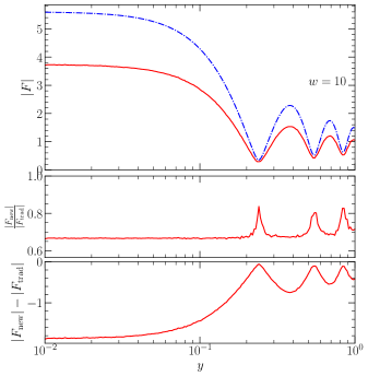
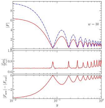
Figure 3: $|F|$ as the function of $y$ with different $w$ values, where the legends are similar to Figure 2.

If the frequency of GW is constant, for example, the GW source is a uniformly rotating NS with emitting continuous GW. In this case, the frequency $w$ is constant, but if the GW source is moving, $y$ is varying, thus amplification factor $F$ is changing with $y$. Thus we show the amplification factor $F(w,y)$ as the function of dimensionless source position $y$ in Figure 3 by assuming the same parameters as Section 2.3.2.

In Figure 3, each subfigure represents a different $w$, which is marked at the top right corner of each subfigure. All legends are similar to Figure 2. The blue dot-dash (red solid)line represents $|F_{\rm trad}|$ ($|F_{\rm new}|$) calculated by traditional (new) diffraction integral. In each subfigure, we can see that the $|F|$ is also oscillating with $y$, especially when $y$ is high. But the oscillation amplitude is decreasing with increasing $y$ and it becomes maximum when $y=0$. The red line is also significantly higher than the blue line. In the middle panel of each subfigure, we can see that $\frac{|F_{\rm new}|}{|F_{\rm trad}|}$ is also basically a constant except some nodes (since $w\geq 1$). At these nodes, $|F_{\rm new}|$ and $|F_{\rm trad}|$ reach local minimums, while the ratio $\frac{|F_{\rm new}|}{|F_{\rm trad}|}$ reaches local maximums, and the absolute value of difference $\left||F_{\rm new}|-|F_{\rm trad}|\right|$ reaches local minimums.

3.3 Light curve examples

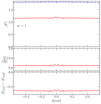
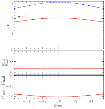
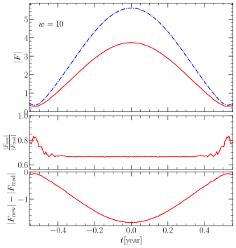
Figure 4: Magnification light curves or $|F|$ as the function of time $t$ with different $w$, where the legends are similar to Figure 2.

Now we consider a more specific example, for instance, a binary system consists of $M_{\rm L}=1M_{\odot}$ star (or white dwarf, NS, etc.) as lens and a rotating asymmetric NS with mass $\sim 1M_{\odot}$ as a GW source. We assume that the binary sysem is edge-on to us. The position of source relative to lens is $\eta=a\sin\omega_{\star}t$, where $a$ is the radius of the binary orbit, $\omega_{\star}$ is the angular velocity of the binary. According to the Kepler’s third law $GM=\omega_{\star}^{2}a^{3}$, we can work out $\omega_{\star}=\sqrt{\frac{GM}{a^{3}}}$ if semimajor axis $a$ is given. Since the binary is always rotating around each other, the GW source is not always eclipsed by its companion. We just consider when the phase angle of the binary is in a small range $-\frac{\pi}{4}<\omega_{\star}t<\frac{\pi}{4}$. Within this range, we can make some approximations. Although $D_{\rm L}$, $D_{\rm LS}$ and $D_{\rm S}$ are varying with time $t$, they are still at the same order of magnitude even for $D_{\rm LS}$ when $-\frac{\pi}{4}<\omega_{\star}t<\frac{\pi}{4}$. For convenience, we ignore their variations within this range. It is clear that $y=\frac{D_{\rm L}}{\xi_{0}D_{S}}\eta=\frac{D_{\rm L}}{\xi_{0}D_{S}}a\sin\sqrt{\frac{GM}{a^{3}}}t$, which is close to linear relation $y\propto t$. Assuming that $D_{\rm L}\simeq D_{\rm S}\sim 1$ kpc$\gg a=D_{\rm LS}\sim 1$ AU, Schwarzschild radius $R_{\rm S}=3$ km for the lens, we show the amplification factor $F(w,y)$ as the function of time $t$, which is similar to light curve in microlensing of EM wave.

Here we assume lens model as point mass model. If the lens is a star, when source position $y$ is within the angular radius of the star, the amplification factor of lens is affected by the density profile of lens [32, 23].

Figure 4 shows $|F|$ as the function of time $t$, i.e. light curve. $|F|$ is oscillating with time $t$, especially when $|t|$ is high, and it becomes maximum when $t=0$, i.e. $y=0$. Its shape is very similar to $|F|$ as the function of $y$ (Figure 3, but its horizontal coordinate is in logarithmic coordinate) and our results are also similar to the results in [29]. Similar to Figure 3, the blue dot-dash (red solid) line represents $|F_{\rm trad}|$ ($|F_{\rm new}|$) calculated by traditional (new) diffraction integral. The red line is also significantly higher than the blue line. And we can draw similar conclusions with Figure 3.

3.4 Ratio $r_{F}$ as the function of $D_{\rm LS}$

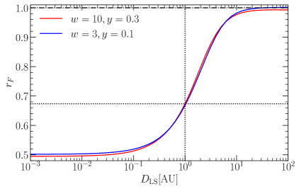
Figure 5: Ratio $r_{F}$ as function of $D_{\rm LS}$. Different colors represent that they have different parameters $w$ and $y$ as shown in the left upper legends. We have chosen two groups of $w$ and $y$ values.

In the previous examples, we all assume the same lens and source distance parameters $D_{\rm L}\simeq D_{\rm S}\sim 1$ kpc$\gg D_{\rm LS}\sim 1$ AU. It is unclear what if these distances are not fixed, but changeable. In this subsection, we consider the influence of lens and source distance on amplification factor $|F|$ (Eq. 2.2).

According to the expressions of $\cos\theta$ and $\cos\theta^{\prime}$ (after Eq. 2.2 or Eq. 2.4), only $\frac{D_{\rm L}}{\xi_{0}}$, $\frac{D_{\rm LS}}{\xi_{0}}$ and $\frac{D_{\rm S}}{D_{\rm L}}$ three ratios will influence the value of $\cos\theta$ and $\cos\theta^{\prime}$. $\frac{D_{\rm L}}{\xi_{0}}\gg 1$ is always a large number even for sun (as we discussed in Sec. 2.3.1), thus the value of this ratio $\frac{D_{\rm L}}{\xi_{0}}$ will not influence the value of $\cos\theta$ and $\cos\theta^{\prime}$. For binary system, we still have $D_{\rm L}\simeq D_{\rm S}\gg D_{\rm LS}$. Thus the ratio $D_{\rm S}/D_{\rm L}\simeq 1$ always works, no matter how much the value of distances $D_{\rm L}$ and $D_{\rm S}$ are. Hence the concrete values of distances $D_{\rm L}$ and $D_{\rm S}$ will not influence the values of $\cos\theta$ and $\cos\theta^{\prime}$. Only the value of $D_{\rm LS}$ will influence the values of $\cos\theta$ and $\cos\theta^{\prime}$. Therefore, we mainly consider the influence of variation of $D_{\rm LS}$ on amplification factor $|F_{\rm new}|$.

The difference between the new and traditional diffractive integral formula is the factor $\frac{(\cos\theta+\cos\theta^{\prime})\cos\theta}{2}$ in the integrand. In previous sections, we find that the ratio of amplification factor $\frac{|F_{\rm new}|}{|F_{\rm trad}|}$ is basically a constant $r_{F}$ except neighbourhoods around each node.

Thus the ratio of module of amplification factors $r_{F}$ can reflect the difference between the new and traditional diffractive integral formula. We assume the same parameters as Section 2.3.2 except $D_{\rm LS}$, and estimate the ratio of amplification factors $r_{F}$ as the function of distance $D_{\rm LS}$ for different $w$ and $y$, and show them in the Figure 5. The positions of $w$ and $y$ are not close to these nodes, thus these $r_{F}$ values can actually reflect more general cases with different parameters. When $D_{\rm LS}=1$ AU, $r_{F}\simeq 0.674$, which is the ratio as shown in previous sections. We can see that $r_{F}$ increases from $\frac{1}{2}$ to $1$ with increasing $D_{\rm LS}$. When $D_{\rm LS}<0.01$ AU, $r_{F}\simeq 0.5$; When $D_{\rm LS}>10$ AU, $r_{F}\simeq 1$. This is because with increasing $D_{\rm LS}$, the average value of $\cos\theta^{\prime}$ increases from 0 to 1, thus the factor $\frac{(\cos\theta+\cos\theta^{\prime})\cos\theta}{2}$ increases from $\frac{1}{2}$ to 1, where $\cos\theta^{\prime}\simeq 1$. In short, when $D_{\rm LS}<10$ AU, the difference between new and traditional diffractive integral formula could be significant.

3.5 Ratio $r_{F}$ as the function of $R_{\rm S}$

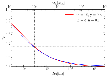
Figure 6: Ratio $r_{F}$ as function of $R_{\rm S}$. And the upper horizontal axis represents the corresponding lens mass $M_{\rm L}$. The legends are similar to Figure 5.

Besides $D_{\rm LS}$, the Schwarzschild radius $R_{\rm S}$ of lens will also influence $r_{F}$. However, $r_{F}$ is not so sensitive to the variation of $R_{\rm S}$. Similar to Figure 5, we show the ratio $r_{F}$ as the function of Schwarzschild radius $R_{\rm S}$ (or lens mass $M_{\rm L}$) for different $w$ and $y$ in the Figure 6. Here only $R_{\rm S}$ is variable, $w$ and $y$ are shown in the legends, other parameters are the same as Section 2.3.2. If $R_{\rm S}$ of lens is larger or lens is more massive, $r_{F}$ is smaller, thus the difference between new and traditional formula is more significant. The value of $r_{F}$ is always between 0.5 and 1. When lens mass $M_{\rm L}\gtrsim 10^{3}M_{\odot}$, $r_{F}\simeq 0.5$. When $M_{\rm L}=0.1M_{\odot}$, $r_{F}$ is still less than 1.

4 Discussion

Firstly, the event number of such kind of binary system (e.g. accreting NS eclipsed by companion) is huge, it can reach $10^{3}-10^{4}$ even more as show in [32] for Milky Way. Although the current GW detectors have not yet observed the continuous GW from rotating NS, it is probable to detect such type of GW sources for the next generation GW detectors, e.g. Cosmic Explorer and Einstein Telescope.

Secondly, the magnification difference is also enough significant to be detected. As discussed in [32], when $\frac{\delta h}{h}>\frac{1}{\varrho}$, where $\varrho$ is the signal to noise ratio (SNR) of GW signal. For a GW signal with $\varrho=8$, as long as the relative strain difference $\frac{\delta h}{h}>\frac{1}{8}$, the difference is detectable for this GW signal. According to our calculational results, the relative magnification difference between new and traditional diffractive formulas is significant because $r_{F}\simeq 0.674$, which means $\Delta h/h\simeq 0.326>\frac{1}{8}$, for $D_{\rm LS}=1$ AU. According to Figure 5, as long as $D_{\rm LS}\lesssim 3$ AU, the relative magnification difference is enough significant to be distinguish for GW signal with SNR $\varrho\geq 8$. If SNR of GW signal could be higher, the detetctable condition could be weaker. If lens mass $M_{\rm L}$ (or $R_{\rm S}$) is variable, as long as $M_{\rm L}\gtrsim 0.1M_{\odot}$, the relative magnification difference is enough significant to be distinguish for GW signal with SNR $\varrho\geq 8$.

Thirdly, the nature of GW is tensor wave, not scalar wave. If the angle between lens and source is great, the polarization tensor of GW could not be regarded as a constant. Our new diffractive formula could be also inaccurate to describe GW with the nature of tensor wave in this case, but it could serve as an approximation formula which is an intermediate transition formula between traditional diffractive formula and tensor diffractive formula. We need to consider the tensor diffractive formula [36] and its polarizations [37] in future work. He et al. [38, 39, 40] simulates GL system of GW in their paper. In order to obtain more accurate lensed GW waveform under such cases and check the accuracy of our diffractive formula, more simulations and researches need to be done on this kind of binary system, i.e., GW sources lensed by its companion.

Fourthly, not only such kind of binary system contains a GW source, but also itself emits GW. The GW from wide binary inspiral could be weak and its frequency is different from (e.g., much lower than) the GW from a component in this binary system, thus it is possible to distinguish two kinds of different GWs from frequency.

In addition, our new diffractive formula can be tested by not only lensed GW, but also lensed EM wave observation. For example, it can be also tested by lensed fast radio burst [41]. If a fast radio burst source, gamma ray burst or a star (light source) eclipsed or lensed by its companion could become an important probe to test our new diffractive formula. Although it could be dominant by geometrical optics for lensed light, there could not exist significant difference between new and traditional diffractive formulas under high frequency limit. More investigations need to be done in related fields.

What is more, our new diffractive formula can be also used to describe the diffraction of a scalar wave, e.g. an ultralight scalar field with long wavelength. For scalar wave, it is accurate to describe such lensed wave system with this formula.

5 Conclusions

In previous work [26], we proposed a new and general diffractive integral formula, which contains large angle diffraction case. We find that when the GW source is lensed or eclipsed by its companion, the difference between new and traditional diffractive integral is significant. Therefore, the GW source lensed by its companion (like NS-compact object binary or accreting NS eclipsed by its companion) can serve as a test of this new diffractive integral. Such binary should be very common in our universe. They are promising to be detected by next-generation GW detectors.

What is more, we have shown how much the difference bewtween new and traditional diffractive integral is for different $w$ and $y$. The module of amplification factor for general diffractive formula is bacsically smaller than that of traditional one. And their ratio $\frac{|F_{\rm new}|}{|F_{\rm trad}|}$ is basically a constant $r_{F}$ except some node points. When the distance between lens and sources is $D_{\rm LS}=1$ AU and lens mass is $M_{\rm L}=1M_{\odot}$, the proportionality factor is $r_{F}\simeq 0.674$. What is more, the value of this factor $r_{F}$ depends on $D_{\rm LS}$ and lens mass $M_{\rm L}$ (or Schwarzschild radius of lens $R_{\rm S}$). If we assume lens mass $M_{\rm L}=1M_{\odot}$, when $D_{\rm LS}<0.01$ AU, $r_{F}\simeq 0.5$; when $0.01{\rm AU}<D_{\rm LS}<10$ AU, $r_{F}$ increases from 0.5 to 1 with increasing $D_{\rm LS}$; when $D_{\rm LS}>10$ AU, $r_{F}\simeq 1$. Only if $D_{\rm LS}<10$ AU, the difference between new and traditional diffractive integral formula could be significant. When $D_{\rm LS}<3$ AU, their difference is enough significant to be detectable for any GW signal with $\varrho>8$. If we fix $D_{\rm LS}=1$ AU, $r_{F}$ is decreasing with increasing $M_{\rm L}$. And when $M>10^{3}M_{\odot}$, $r_{F}\simeq 0.5$. When $M_{\rm L}>0.1M_{\odot}$, their difference is enough significant to be detectable for any GW signal with $\varrho>8$. This new general diffractive formula is hopeful to be tested by next-generation GW detectors in the future GW detection.

Appendix A Phase difference in lensing

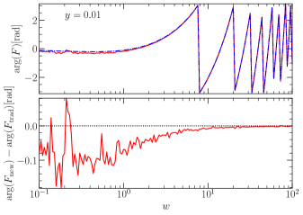
Figure 7: Phase of amplification factor $\arg(F)$ from new (red solid line) and traditional (blue dot-dash line) diffractive integrals and their phase difference (bottom panel).

Similar to Figure 2, we also show phase of amplification factor $\arg(F)$ as the function of frequency $w$ in Figure 7. For simplicity, we assume $\phi_{m}(y)\equiv 0$ in the calculation of value of absolute phase $\arg(F)$. The absolute phase is not important, but the phase difference between them matters. The phase difference $\Delta\Phi=\arg(F_{\rm new})-\arg(F_{\rm trad})$ between the new formula and traditional one is very small. The absolute value of phase difference is basically less than 0.1 rad. And when $w\rightarrow\infty$, phase difference $\Delta\Phi=\arg(F_{\rm new})-\arg(F_{\rm trad})\rightarrow 0$. Thus the phase difference is not significant for all kinds of values of $w$ and $y$ at least for $w<100$.

References

- [1] P. Schneider, J. Ehlers and E.E. Falco, Gravitational Lenses, Springer-Verlag New York (1992), 10.1007/978-3-662-03758-4.
- [2] Gravitational Lensing: Strong, Weak and Micro, Springer Berlin, Heidelberg, Jan., 2006.
- [3] C.W. Misner, K.S. Thorne and J.A. Wheeler, Gravitation, Physics Series, W. H. Freeman, first edition ed. (1973).
- [4] M. Maggiore, Gravitational waves: Volume 1: Theory and experiments, Oxford University Press, Oxford (2008).
- [5] LIGO Scientific Collaboration and Virgo Collaboration collaboration, Observation of Gravitational Waves from a Binary Black Hole Merger, Phys. Rev. Lett. 116 (2016) 061102 [1602.03837].
- [6] LIGO Scientific Collaboration and Virgo Collaboration collaboration, Tests of general relativity with the binary black hole signals from the LIGO-Virgo catalog GWTC-1, Phys. Rev. D 100 (2019) 104036 [1903.04467].
- [7] LIGO Scientific Collaboration and Virgo Collaboration collaboration, Tests of general relativity with binary black holes from the second LIGO-Virgo gravitational-wave transient catalog, Phys. Rev. D 103 (2021) 122002 [2010.14529].
- [8] LIGO Scientific Collaboration and Virgo Collaboration collaboration, Search for Lensing Signatures in the Gravitational-Wave Observations from the First Half of LIGO-Virgo’s Third Observing Run, Astrophys. J. 923 (2021) 14 [2105.06384].
- [9] L. Dai, B. Zackay, T. Venumadhav, J. Roulet and M. Zaldarriaga, Search for Lensed Gravitational Waves Including Morse Phase Information: An Intriguing Candidate in O2, arXiv e-prints (2020) arXiv:2007.12709 [2007.12709].
- [10] T.E. Collett and D. Bacon, Testing the Speed of Gravitational Waves over Cosmological Distances with Strong Gravitational Lensing, Phys. Rev. Lett. 118 (2017) 091101 [1602.05882].
- [11] X.-L. Fan, K. Liao, M. Biesiada, A. Piórkowska-Kurpas and Z.-H. Zhu, Speed of Gravitational Waves from Strongly Lensed Gravitational Waves and Electromagnetic Signals, Phys. Rev. Lett. 118 (2017) 091102 [1612.04095].
- [12] K. Liao, X.-L. Fan, X. Ding, M. Biesiada and Z.-H. Zhu, Precision cosmology from future lensed gravitational wave and electromagnetic signals, Nature Communications 8 (2017) 1148 [1703.04151].
- [13] Z. Chen, Y. Lu and Y. Zhao, Constraining the Origin of Stellar Binary Black Hole Mergers by Detections of Their Lensed Host Galaxies and Gravitational Wave Signals, Astrophys. J. 940 (2022) 17 [2210.09892].
- [14] L. Dai, S.-S. Li, B. Zackay, S. Mao and Y. Lu, Detecting lensing-induced diffraction in astrophysical gravitational waves, Phys. Rev. D 98 (2018) 104029 [1810.00003].
- [15] M. Oguri and R. Takahashi, Probing Dark Low-mass Halos and Primordial Black Holes with Frequency-dependent Gravitational Lensing Dispersions of Gravitational Waves, Astrophys. J. 901 (2020) 58 [2007.01936].
- [16] K. Liao, S. Tian and X. Ding, Probing compact dark matter with gravitational wave fringes detected by the Einstein Telescope, Mon. Not. Roy. Astron. Soc. 495 (2020) 2002 [2001.07891].
- [17] H.G. Choi, C. Park and S. Jung, Small-scale shear: Peeling off diffuse subhalos with gravitational waves, Phys. Rev. D 104 (2021) 063001.
- [18] X. Guo and Y. Lu, Probing the nature of dark matter via gravitational waves lensed by small dark matter halos, Phys. Rev. D 106 (2022) 023018 [2207.00325].
- [19] G. Tambalo, M. Zumalacárregui, L. Dai and M. Ho-Yeuk Cheung, Gravitational wave lensing as a probe of halo properties and dark matter, arXiv e-prints (2022) arXiv:2212.11960 [2212.11960].
- [20] M. Fairbairn, J. Urrutia and V. Vaskonen, Microlensing of gravitational waves by dark matter structures, J. Cosmol. Astropart. P. 2023 (2023) 007 [2210.13436].
- [21] M. Çalışkan, N.A. Kumar, L. Ji, J.M. Ezquiaga, R. Cotesta, E. Berti et al., Probing wave-optics effects and dark-matter subhalos with lensing of gravitational waves from massive black holes, arXiv e-prints (2023) arXiv:2307.06990 [2307.06990].
- [22] S. Jung and S. Kim, Solar diffraction of LIGO-band gravitational waves, J. Cosmol. Astropart. P. 2023 (2023) 042 [2210.02649].
- [23] R. Takahashi, S. Morisaki and T. Suyama, Probing the Solar Interior with Lensed Gravitational Waves from Known Pulsars, Astrophys. J. 957 (2023) 52 [2304.08220].
- [24] R. Takahashi, Wave Effects in the Gravitational Lensing of Gravitational Waves from Chirping Binaries, Ph.D. thesis, Kyoto University, Jan., 2004.
- [25] T.T. Nakamura and S. Deguchi, Wave Optics in Gravitational Lensing, Progress of Theoretical Physics Supplement 133 (1999) 137.
- [26] X. Guo and Y. Lu, Convergence and efficiency of different methods to compute the diffraction integral for gravitational lensing of gravitational waves, Phys. Rev. D 102 (2020) 124076 [2012.03474].
- [27] R. Takahashi and T. Nakamura, Wave Effects in the Gravitational Lensing of Gravitational Waves from Chirping Binaries, Astrophys. J. 595 (2003) 1039 [astro-ph/0305055].
- [28] Z. Cao, L.-F. Li and Y. Wang, Gravitational lensing effects on parameter estimation in gravitational wave detection with advanced detectors, Phys. Rev. D 90 (2014) 062003.
- [29] K. Liao, M. Biesiada and X.-L. Fan, The Wave Nature of Continuous Gravitational Waves from Microlensing, Astrophys. J. 875 (2019) 139 [1903.06612].
- [30] H. Ma, Y. Lu, Z. Chen and Y. Chen, Diffractive lensing of nano-Hertz gravitational waves emitted from supermassive binary black holes by intervening galaxies, Mon. Not. R. Astron. Soc. 524 (2023) 2954 [2307.02742].
- [31] R.N. Manchester, G.B. Hobbs, A. Teoh and M. Hobbs, The Australia Telescope National Facility Pulsar Catalogue, Astron. J. 129 (2005) 1993 [astro-ph/0412641].
- [32] P. Marchant, K. Breivik, C.P.L. Berry, I. Mandel and S.L. Larson, Eclipses of continuous gravitational waves as a probe of stellar structure, Phys. Rev. D 101 (2020) 024039 [1912.04268].
- [33] A. Ulmer and J. Goodman, Femtolensing: Beyond the Semiclassical Approximation, Astrophys. J. 442 (1995) 67 [astro-ph/9406042].
- [34] D. Levin, Procedures for Computing One- and Two-Dimensional Integrals of Functions With Rapid Irregular Oscillations, Mathematics of Computation 38 (1982) 531.
- [35] A.J. Moylan, D.E. McClelland, S.M. Scott, A.C. Searle and G.V. Bicknell, Numerical Wave Optics and the Lensing of Gravitational Waves by Globular Clusters, in The Eleventh Marcel Grossmann Meeting On Recent Developments in Theoretical and Experimental General Relativity, Gravitation and Relativistic Field Theories, pp. 807–823, Sept., 2008, DOI [0710.3140].
- [36] S. Hou, X.-L. Fan and Z.-H. Zhu, Gravitational lensing of gravitational waves: Rotation of polarization plane, Phys. Rev. D 100 (2019) 064028 [1907.07486].
- [37] Z. Li, J. Qiao, W. Zhao and X. Er, Gravitational Faraday Rotation of gravitational waves by a Kerr black hole, J. Cosmol. Astropart. P. 2022 (2022) 095 [2204.10512].
- [38] J.-h. He, Unveiling the wave nature of gravitational-waves with simulations, arXiv e-prints (2020) arXiv:2005.10485 [2005.10485].
- [39] J.-h. He, GWSIM: a code to simulate gravitational waves propagating in a potential well, Mon. Not. R. Astron. Soc. 506 (2021) 5278 [2107.09800].
- [40] Y. Qiu, K. Wang and J.-h. He, Amplitude modulation in binary gravitational lensing of gravitational waves, arXiv e-prints (2022) arXiv:2205.01682 [2205.01682].
- [41] D.L. Jow, S. Foreman, U.-L. Pen and W. Zhu, Wave effects in the microlensing of pulsars and FRBs by point masses, Mon. Not. R. Astron. Soc. 497 (2020) 4956 [2002.01570].