Confined run and tumble particles with non-Markovian tumbling statistics

Abstract

Confined active particles constitute simple, yet realistic, examples of systems that converge into a non-equilibrium steady state. We investigate a run-and-tumble particle in one spatial dimension, trapped by an external potential, with a given distribution $g(t)$ of waiting times between tumbling events whose mean value is equal to $\tau$. Unless $g(t)$ is an exponential distribution (corresponding to a constant tumbling rate), the process is non-Markovian, which makes the analysis of the model particularly challenging. We use an analytical framework involving effective position-dependent tumbling rates, to develop a numerical method that yields the full steady-state distribution (SSD). The method is very efficient and requires modest computing resources, including in the large-deviations and/or small-$\tau$ regime, where the SSD can be related to the the large-deviation function, $s(x)$, via the scaling relation $P_{{\rm st}}(x)\sim e^{-s\left(x\right)/\tau}$.

I Introduction

Active particles Romanczuk ; soft ; BechingerRev ; FodorEtAl15 ; Fodor16 ; Needleman17 ; Ramaswamy2017 ; Marchetti2017 ; Schweitzer ; FJC22 , in contrast with their passive Brownian counterparts, use energy that they pump out of their environment in order to move. Activity leads to breaking of time-reversal symmetry, and as a result, even single active particles are out of (thermal) equilibrium. Many natural examples of active systems may be found in biology, from molecular motors BHG06 ; Toyota11 ; Stuhrmann12 ; Mizuno07 to cells Berg2004 ; Wilhelm08 ; Cates2012 ; Ahmed15 ; BeerEtAl20 ; Breoni22 ; Nishiguchi23 , to animals flocking1 ; flocking2 ; Vicsek ; fish . Moreover, active systems have been experimentally realized and studied. This has been done by fabricating artificial particles (such as Janus particles) or robots that propel themselves BechingerRev ; Hagen2014 ; Takatori2016 ; Deblais2018 ; Dauchot2019 ; gran2 ; GLA07 ; PBDN21 ; BCASL22 ; MolodtsovaEtAl23 ; PPSK23 ; Nishiguchi23 leading to behavior which is similar to that of the natural examples.

The statistical behavior of active systems may be quite remarkable indeed, and very different to the equilibrium behavior exhibited by passive systems, both for active, many-body systems (“active matter”) separation1 ; separation2 ; separation3 ; cluster1 ; cluster2 ; evans ; Kardar2015 ; PBV19 ; Singh21 ; ARYL21 ; Cates22 ; ARYL23 ; SSB22 ; ACJ22 and even at the single particle level Wensink2008 ; Elgeti2009 ; gran2 ; Li2009b ; TC08 ; Kaiser2012 ; Elgeti2013 ; Hennes2014 ; Solon2015 ; Takatori2016 ; Li2017 ; Razin2017 ; Dauchot2019 ; Pototsky2012 ; Solon2015 ; Pototsky2012 ; TC08 ; ABP2019 ; Dhar_2019 ; Malakar20 ; Franosch2016 ; Das2018 ; Caprini2019 ; Sevilla2019 ; Hagen2014 ; Takatori2016 ; Deblais2018 ; Dauchot2019 ; SBS21 ; MalakarEtAl18 ; ABP2018 ; Singh2019 ; SmithFarago22 ; SLMS22RTP ; Smith2023 ; Frydel24 ; BM24 . A setting that has attracted much recent interest is that of a single active particle trapped by an external potential. Such a particle eventually reaches a nonequilibrium steady state that differs from the Boltzmann-Gibbs statistics Solon2015 ; Pototsky2012 ; TC08 ; ABP2019 ; Dhar_2019 ; Malakar20 ; Franosch2016 ; Das2018 ; Caprini2019 ; Sevilla2019 ; Hagen2014 ; Takatori2016 ; Deblais2018 ; Dauchot2019 ; SBS21 ; SmithFarago22 ; SLMS22RTP ; Smith2023 ; Frydel24 , its first-passage properties do not follow the Arrhenius law MalakarEtAl18 ; ABP2018 ; Singh2019 , and it may acquire an effective drift even if it is placed in a periodic potential led20 .

The nonequilibrium nature of active matter makes its analytical study very challenging. Some relatively simple models admit exact solutions. One example is the run-and-tumble particle (RTP), which, in the absence of external forces, moves at a constant speed but changes its orientation at a constant rate. In one dimension, the RTP model is exactly solvable with Kardar2015 ; Dhar_2019 or without wei02 ; HV_2010 ; ODA_1988 ; MADB_2012 ; MalakarEtAl18 ; EM_2018 ; Dhar_2019 ; SBS20 ; Dean21 an external potential, and in some special cases, these results may be extended to higher dimensions SLMS22RTP ; ABP2018 ; Malakar20 ; SBS20 ; CO21 ; Frydel22 . In some less simple settings, active systems are amenable to a perturbative treatment in various regimes MB20 ; SmithFarago22 ; SBS21 ; Smith2023 . However, in many cases one must resort to numerical methods. The challenge posed by active systems becomes especially pronounced when studying large deviations (i.e., rare events), which often cannot be studied by brute-force Langevin dynamics simulations. Large-deviations have become a major theme of ongoing interest in statistical mechanics DZ ; Hollander ; Majumdar2007 ; hugo2009 ; Derrida11 ; MajumdarSchehr2017 ; Touchette2018 , because they are often very strongly affected by the activity of the system, while the effects on the typical-fluctuations may be weaker.

In a vast majority of previous works, the stochastic dynamics of active particles that were studied were assumed to be Markovian. By this we mean that the particle’s instantaneous position and internal state (e.g., for an RTP the internal state is its orientation) contain sufficient information to predict the statistics of its future dynamics, and it is not necessary to know the full history of the particle’s dynamics (see footnote footnote1 ). Markovian dynamics are “memory-free”, and the Markovian assumption facilitates the analysis considerably, but it also restricts the class of models that may be analyzed. It is also not so obvious if this assumption indeed holds for realistic systems, such as living cells, for which one may reasonably expect that some effects of memory are present.

In the present work, we consider an RTP with a given distribution $g(t)$ of waiting times between tumbling events, with mean waiting time $\tau$. The particular case where $g(t)$ is an exponential distribution corresponds to a constant tumbling rate, recovering the standard (Markovian) RTP model. For any non-exponential $g(t)$, the model becomes non Markovian, and very challenging to study. Our model may be thought of as an extension of the continuous-time random walk model, whose large-deviations properties have attracted much interest recently WBB20 ; SB23 . In order to study the model, we develop a numerical method which allows to compute the nonequilibrium steady state distribution (SSD) of the particle, including in the regime of large deviations and/or small $\tau$. Many of the existing large-deviations numerical methods are based on generating realizations of the stochastic process under study that are biased toward the rare event of interest Hartmann2002 ; TL09 ; HG11 ; touchette2011 ; Claussen2015 ; Hartmann2018 ; GV19 ; Hartmann2019LIS ; Hartmann2019 ; Hartmann2020 ; HartmannMS2021 ; CBG23 ; SmithChaos22 ; SmithFarago22 ; NickelsenTouchette22 . In contrast, our method circumvents the need to generate realizations of the process, while relying on some theoretical insights that we derive. It should thus be viewed as a combined theoretical and numerical framework.

The remainder of the paper is organized as follows. In section II we define the non-Markovian RTP model precisely, and introduce the key theoretical concepts for studying the nonequilibrium steady state that is reached when this particle is placed in a trapping potential. In section III we use these concepts to describe the numerical method by which the steady state can be computed. In section IV we present results that we obtained using this method for three particular waiting time distributions $g(t)$: Exponential (which serves as a benchmark to verify that our results agree with the known, exact solution), semi-Gaussian, and half-t. In section V we summarize and discuss our main findings.

II Model definition and theoretical framework

We consider an overdamped particle moving in a one-dimensional (1D) potential field $U(x)$. For simplicity we assume that $U(x)$ is mirror symmetric $U(x)=U(-x)$, and has a unique minimum at $x=0$. The particle is subject to an active telegraphic (dichotomous) noise that switches between two values $\sigma(t)=\pm\sigma_{0}$. This is known as the 1D run-and-tumble particle (RTP) model. We further assume that the running times [i.e., the times between consecutive switching events of the sign of $\sigma(t)$] are drawn from a general distribution $g(t)$ [$\int_{0}^{\infty}g(t)dt=1$]. We denote the mean running time by $\tau=\int_{0}^{\infty}tg(t)dt$. The most thoroughly studied case is when $g(t)=\exp(-t/\tau)/\tau$, for which $\sigma(t)$ is (time-independent) tumbling (switching) rate $\gamma=1/\tau$. For any other distribution function, $g(t)$, the process is non-Markovian.

The Langevin equation describing the dynamics of the particle is

$$\mu\dot{x}-F(x)-\sigma(t)=0,$$ (1)

where $\mu$ is the friction coefficient, and $F(x)=-U^{\prime}(x)$. Since the particle has no inertia, it is confined to the interval $-X_{0}<x<X_{0}$, where $|F(X_{0})|=\sigma_{0}$ [assuming that such $X_{0}$ exists, and that $-X_{0}<x(t=0)<X_{0}$]. Its instantaneous direction of motion is that of $\sigma(t)$, and for a given orientation, the speed is an injective function of $x$ given by

$$\mu v_{\pm}(x)=\sigma_{0}\pm F(x),$$ (2)

where the subscripts $\pm$ denote the speeds when the particle moves in the positive and negative directions, respectively.

Here, we introduce a theoretical-numerical framework for calculating the SSD of the particle, $P_{\rm st}(x)$. Our approach is not based on straightforward Langevin dynamics simulations, which tend to be inefficient in the large-deviation regime $|x|\lesssim X_{0}$, especially when $\tau$ is small. Instead, we begin the analysis by considering the probability flux which is constant at steady-state, $J_{\rm st}(x)=J$. Since the particle is confined to a finite interval, we have that $J_{\rm st}=0$. In what follows, we consider the steady-state statistics of the particle and, therefore, drop the subscript “st” for brevity.

II.1 Steady-state currents

The steady-state flux is the difference between the currents of particles moving in the positive and negative directions, $J(x)=I_{+}(x)-I_{-}(x)$. We denote by $P_{+}(x)$ and $P_{-}(x)$ the distributions corresponding, in steady-state, to right- and left-moving particles, respectively. These are related to the SSD $P(x)$ via

$$P(x)=P_{+}(x)+P_{-}(x),$$ (3)

and because of the symmetry of the problem, both of them are normalized to $\int_{-\infty}^{\infty}P_{\pm}\left(x\right)dx=1/2$ (rather than unity), and satisfy $P_{+}(x)=P_{-}(-x)$. The associated currents are given by $I_{\pm}(x)=P_{\pm}(x)v_{\pm}(x)$. Since $J=0$, we have that $I_{+}(x)=I_{-}(x)$, and so we adopt the same notation $I(x)$ for both, i.e.,

$$I(x)=P_{+}(x)v_{+}(x)=P_{-}(x)v_{-}(x).$$ (4)

We now arrive at a key part of the derivation, which is the introduction of the space-dependent effective switching rates, $\gamma_{\pm}(x)$. These rates express the probability, per unit time, of a particle to tumble (i.e., flip its orientation) when traveling in the vicinity of $x$. We denote by $i_{\pm}^{t}(x)$, the associated tumbling current densities (per unit length per unit time)

$$i_{\pm}^{t}(x)=\gamma_{\pm}(x)P_{\pm}(x),$$ (5)

which from Eq. (4) can be also written as

$$i_{\pm}^{t}(x)=I(x)\frac{\gamma_{\pm}(x)}{v_{\pm}(x)}.$$ (6)

Due to the occasional switches in the direction of motion, the current changes, over a small distance $dx$, by $dI(x)=\left[i_{-}^{t}(x)-i_{+}^{t}(x)\right]dx$. Thus, we arrive at the differential equation

$$\frac{dI}{dx}=I(x)\left[\frac{\gamma_{-}(x)}{v_{-}(x)}-\frac{\gamma_{+}(x)}{v_{+}(x)}\right],$$ (7)

with the solution

$$I(x)=I(x=0)\exp\left\{\int_{0}^{x}\left(\frac{\gamma_{-}(y)}{v_{-}(y)}-\frac{\gamma_{+}(y)}{v_{+}(y)}\right)dy\right\}.$$ (8)

From Eqs. (3) and (4), we have that

$$P(x)=I(x)\left(\frac{1}{v_{+}(x)}+\frac{1}{v_{-}(x)}\right).$$ (9)

Furthermore, because $F(0)=0$, we have from Eq. (2) that $v_{\pm}(0)=\sigma_{0}/\mu$, and we thus arrive at the result that

$$\frac{P(x)}{P(x=0)} = \frac{\sigma_{0}^{2}}{\sigma_{0}^{2}-F^{2}(x)}\times$$

$$\exp \left\{\mu\int_{0}^{x}\left(\frac{\gamma_{-}(y)}{\sigma_{0}-F(y)}-\frac{\gamma_{+}(y)}{\sigma_{0}+F(y)}\right)dy\right\}.$$

II.2 Relating $\gamma_{\pm}(x)$ to $g(t)$

A derivation similar to the one presented in the previous subsection was introduced in Ref. Monthus2021 . However, in that paper the rates $\gamma_{\pm}(x)$ were simply taken to be given functions, i.e., the model studied there was a Markovian RTP with space-dependent tumbling rates (and velocities). In contrast, in our non-Markovian model, $\gamma_{\pm}(x)$ are a-priori unknown, but we can relate them to the function $g(t)$, which characterizes the statistics of switching times.

When $g(t)=\exp(-t/\tau)/\tau$, the switching rates are both time- and space-independent, i.e., $\gamma_{\pm}(x)=\gamma=1/\tau$, and we recover the well-known result q-optics1 ; q-optics2 ; q-optics3 ; q-optics4 ; VBH84 ; colored ; Kardar2015 ; Dhar_2019

$$\frac{P(x)}{P(x=0)} = \frac{\sigma_{0}^{2}}{\sigma_{0}^{2}-F^{2}(x)}\times$$

$$\exp \left\{\frac{2\mu}{\tau}\int_{0}^{x}\left(\frac{F(y)}{\sigma_{0}^{2}-F^{2}(y)}\right)dy\right\}.$$

To proceed in the general case, we introduce the transition probability density per unit length, $\Pi_{+}(a,b)$, that the particle travels directly (i.e., without switching directions in between), starting at point $x=a$ and stopping at point $x=b>a$. Similarly, $\Pi_{-}(a,b)$ denotes the probability density of a movement interval that starts at $x=a$ and ends at $x=b<a$. Due to the symmetry of the problem with respect to $x=0$, it is clear that $\Pi_{+}(a,b)=\Pi_{-}(-a,-b)$. The tumbling current densities (5) satisfy the following set of coupled equations

$$i_{+}^{t}(x) = \int_{-X_{0}}^{x}i_{-}^{t}(y)\Pi_{+}(y,x)dy,$$ (12)

$$i_{-}^{t}(x) = \int_{x}^{+X_{0}}i_{+}^{t}(y)\Pi_{-}(y,x)dy.$$ (13)

These equations are obtained by integrating over the position $y$ of the last tumbling event before the tumbling at position $x$. In order to express the transition probability densities, we consider the traveling time along the interval from from $x=a$ to $x=b$, which is given by

$$t_{+}(a,b)=\int_{a}^{b}\frac{dx}{v_{+}(x)},$$ (14)

if $a<b$, and by

$$t_{-}(a,b)=t_{+}(-a,-b),$$ (15)

if $a>b$. Since the particle always moves at the instantaneous direction of the noise, the probability densities associated with these traveling times are $g[t_{\pm}(a,b)]$. These probability densities per unit time are related to the transition densities per unit length, via

$$\Pi_{\pm}(y,x)=g\left[t_{\pm}\left(y,x\right)\right]\frac{\partial t_{\pm}}{\partial y}=\frac{g\left[t_{\pm}\left(y,x\right)\right]}{v_{\pm}(y)}.$$ (16)

From Eqs. (12), (13), and (16) we find that

$$i_{+}^{t}(x) = \int_{-X_{0}}^{x}i_{-}^{t}(y)\frac{g\left[t_{+}\left(y,x\right)\right]}{v_{+}(y)}dy,$$ (17)

$$i_{-}^{t}(x) = \int_{x}^{X_{0}}i_{+}^{t}(y)\frac{g\left[t_{-}\left(y,x\right)\right]}{v_{-}(y)}dy.$$ (18)

Eqs. (17) and (18) are a set of integral equations for the tumbling current densities $i_{\pm}^{t}(x)$, and they constitute the main results of the theoretical part of our analysis. In these equations, the function $g(t)$ is given and so are $v_{\pm}(x)$, as they are given immediately from the external force $F(x)$ via Eq. (2). Given the solution $i_{\pm}^{t}(x)$ to these equations, one can obtain $I(x)$ by integrating the equation $dI/dx=i_{-}^{t}(x)-i_{+}^{t}(x)$, yielding the steady-state distribution $P(x)$ through Eq. (9). However, solving Eqs. (17) and (18) for general $g(t)$ and $F(x)$ is a highly non-trivial task. In the next section, we present a numerical method for solving these equations.

III The Numerical Scheme

III.1 Computing the tumbling current densities $i_{\pm}^{t}(x)$

The set of integral equations (17)-(18) can be solved numerically. For this purpose, we discretize the support interval $(-X_{0},+X_{0})$ into an even number $N$ of small bins of size $\delta x=2X_{0}/N$. Denoting the end points by $x_{0}=-X_{0}$ and $x_{N}=+X_{0}$, we use the integer variable $i$ to index the bin extending from $x_{i-1}$ to $x_{i}=x_{i-1}+\delta x$. We then determine the travel time between any two points $x_{i}$ and $x_{j}$ for $i,j=1,2,\ldots,N$. This can be done either analytically (if possible) or numerically. Because of the symmetry of the problem, we only consider the travel times in the positive direction. In the case of a numerical integration, it is possible to use Eq. (14) to determine the travel time, $t_{+}(j,i)$, between $x_{j}$ and $x_{i}\geq x_{j}$, but the vanishing of $v_{+}(x)$ close to the edge of the support, $x\lesssim X_{0}$, imposes severe restrictions on the bin size, $\delta x$. Therefore, it is recommended to compute $t_{+}(j,i)$ by numerically integrating the equation of motion (1) with a small integration time-step $\delta t$. Note that in this process, the Langevin equation (1) is not treated as a stochastic, but as a deterministic equation, with $\sigma(t)=+\sigma_{0}$ for a particle moving rightwards.

It is tempting to write the discretized version of Eq. (17) as

$$i_{+}^{t}(x_{i})=\sum_{j=1}^{i}i_{-}^{t}(x_{j})\frac{g\left[t_{+}\left(j,i\right)\right]}{v_{+}(x_{j})}\delta x.$$ (19)

However, similarly to the considerations discussed above regarding the computation of the travel times, we must keep in mind here that Eq. (17) is a re-expression of Eq. (12) where the transition probability per unit length, $\Pi_{+}(y,x)$, is replaced with the transition probability per unit time, $g[t_{+}(y,x)]$. The conversion between them is the origin of the factor $1/v_{+}(y)$ appearing in the integrand in Eq. (17) [see Eq. (16)], which is the inverse ratio between the length of an infinitesimal element around $y$ and the infinitesimal time that the particle spends in that element. This differential form is valid only if the travel time is small, which is not the case when particle approaches the edge of the support $y\lesssim X_{0}$. This problem can be solved by noticing that

$$\int_{x_{i-1}}^{x_{i}}\frac{g\left[t_{+}\left(y,x\right)\right]}{v_{+}(y)}dy = G\left[t_{+}(j,i)\right]-G\left[t_{+}(j,i-1)\right]$$ (20)

$$\equiv \delta G(j,i),$$

where $G(t)=\int_{0}^{t}g(s)ds$ is the cumulative distribution function of the traveling time $t$. We identify the function $\delta G(j,i)$ as the probability of a particle to stop in the $i$-th bin if the movement forward begins at $x_{j}\leq x_{i-1}$. Note that for any $j<N$, $\delta G(j,N)=1-G[t_{+}(j,N-1)/\tau]$, because the travel time to $x_{N}=+X_{0}$ diverges. With these considerations, the discretized version of Eq. (17) is given by

$$i_{+}^{t}(x_{i})=\sum_{j=1}^{i}i_{-}^{t}(x_{j})\delta G(j,i+1),$$ (21)

which holds for $i=1,2,\ldots N-1$ (i.e., excluding the edges $x_{0}=-X_{0}$ and $x_{N}=+X_{0}$). Using the symmetry of the problem $i_{+}^{t}(x)=i_{-}^{t}(-x)$, we rewrite Eq. (21) as

$$p_{+}^{t}(x_{i})=\sum_{j=1}^{i}p_{+}^{t}(x_{N-j})\delta G(j,i+1).$$ (22)

Notice that in the last equation, we replaced the notation $i_{+}^{t}(x_{i})$ with $p_{+}^{t}(x_{i})$. This is done in order to highlight that $p_{+}^{t}(x_{i})$ is the tumbling probability, rather than the tumbling current, of a right-moving particle in the $i$-th bin. In (22), we have a set of $(N-1)$ linear equations which can be solved by various numerical techniques. We use a simple iterative method, starting from the initial state, $p_{+}^{t}(x_{i}^{n})=p_{0}$, and iterating the set of equations until the stationary solution is obtained, typically after several tens of iterations. Notice that the numerically derived probability is not properly normalized but, as we show below, the normalization cancels when we attempt to estimate the switching rates $\gamma(x_{i})$ and the SSD relative to the origin $P_{+}(x_{i})/P_{+}(x_{N/2}=0)$.

III.2 Computing the SSD and the switching rates

From the solution for the tumbling probabilities, $p_{+}^{t}(x_{i})$, we can evaluate the SSD and the switching rates using the following expressions: Similarly to the logic behind the derivation of Eq. (22), it is easy to see that the discretized steady-state distribution is given by

$$P_{+}(x_{i})=\sum_{j=1}^{i}p_{+}^{t}(x_{N-j})\left\{1-G\left[t_{+}\left(j,i\right)\right]\right\}.$$ (23)

After the evaluation of $P_{+}(x_{i})$, the discrete steady-state probability should be normalized to half. Here, we skip this step because we are only interested in the probability relative to the center of the potential well.

While $p_{+}^{t}(x_{i})$ measures the distribution of tumbling points, the ratio $p_{+}^{t}(x_{i})/P(x_{i})$ measures the tumbling probability of a right-moving particle located in the $i$-th bin to tumble during the time interval that it travels through the bin. This quantity is proportional to the switching rate, $\gamma_{+}(x_{i})$. Explicitly, the switching rate is obtained by dividing this ratio by the time, $t_{+}(i-1,i)$, that the particle spends in the bin

$$\gamma_{+}(x_{i})=\frac{1}{t_{+}(i-1,i)}\frac{p_{+}^{t}(x_{i})}{P_{+}(x_{i})}.$$ (24)

This expression is also insensitive to the normalization of $P_{+}(x_{i})$ because, as evident from Eq. (23), the SSD normalization factor is proportional to normalization factor of the tumbling probabilities. Eq. (24) suffers from the same problem encountered in Eq. (19), namely the fact that it assumes that the travel time in the bin is small. This is not the case near the edge of the support where the travel times become increasingly large. Since the tumbling ratio $p_{+}^{t}(x_{i})/P(x_{i})\leq 1$, it implies that Eq. (24) would yield switching rates that become vanishingly small. To fix this problem, we compute the effective switching rate from the following equation

$$\frac{p_{+}^{t}(x_{i})}{P_{+}(x_{i})}=1-\exp\left[-\gamma_{+}(x_{i})t_{+}(i-1,i)\right],$$ (25)

which compares the computed stopping ratio to the corresponding ratio in the case that the switching rate is constant during the travel time [i.e., as if the distribution of running times is exponential with $\tau=1/\gamma_{+}(x_{i})$]. As can be easily seen, Eqs. (24) and (25) coincide in the limit $\gamma_{+}(x_{i})t_{+}(i-1,i)\ll 1$.

IV Computational Results

In this section we present numerical results for several distribution functions, $g(t)$, of the running times. In all cases, we consider a particle in a potential field given by $U(x)=(2/\pi)\{1-\cos[(\pi/2)x]\}$, which means that

$$F(x)=-\sin[(\pi/2)x].$$ (26)

We set the noise amplitude to $\sigma_{0}=1$ and the friction coefficient to $\mu=1.75$. For these parameters, the particle is bound in the interval $|x|<X_{0}=1$, which is discretized into bins of size $\delta x=10^{-3}$. The travel times in the present case can be calculated analytically:

$$t_{+}(j,i) = \mu\int_{x_{j}}^{x_{i}}\frac{dx}{1-\sin[(\pi/2)x]}$$

$$= \frac{2\mu}{\pi}\left\{\tan\left[\frac{\pi}{4}\left(1+x_{i}\right)\right]-\tan\left[\frac{\pi}{4}\left(1+x_{j}\right)\right]\right\}\,.$$

We also measured $t_{+}(j,i)$ numerically, by integration of Langevin equation (1) with time step $\delta t=10^{-6}$. The numerical integration results were in full agreement with Eq. (IV).

As we will see below, the computational method introduced above is not only very accurate including in the large-deviation regime, it is also very efficient and requires very modest computing resources. One only needs to compute the travel time, $t_{+}(j,i)$, between any pair of bins $j\leq i$, which for the simulations presented herein was done on a PC in less than 24 hours of CPU time. Once the times are computed, they can be used for the evaluation of the cumulative function $G[t_{+}(j,i)]$ of any distribution function $g(t)$, and the iterations needed to find the solution of the set of equations (22) take only a few seconds.

IV.1 Exponential distribution (Markov process)

To demonstrate the accuracy of the method, we begin by considering the (exactly-solvable) case $g(t)=\exp(-t/\tau)/\tau$. For this distribution function of travel times, the solution for the SSD is given by Eq. (II.2). Introducing the function

$$s_{\tau}(x)\equiv-\tau\ln\left[\frac{I(x)}{I(x=0)}\right],$$ (28)

we rewrite Eq. (II.2) as

$$\frac{s_{\tau}(x)}{\tau} = -\ln\left[\frac{\sigma_{0}^{2}-F^{2}(x)}{\sigma_{0}^{2}}\frac{P(x)}{P(x=0)}\right]$$

$$= \frac{2\mu}{\tau}\int_{0}^{x}\left(\frac{F(y)}{\sigma_{0}^{2}-F^{2}(y)}\right)dy\,.$$ (29)

We thus find that for the exponential $g(t)$, $s_{\tau}(x)$ is independent of $\tau$, and coincides with the large-deviation-function (LDF) $s(x)$ that describes the SSD in the limit $\tau\to 0$ via $P\left(x\right)\sim e^{-s\left(x\right)/\tau}$ (which is a large-deviations principle) SmithFarago22 ; Smith2023 . For the force function (26), it is given by

$$s(x)=\frac{4\mu}{\pi}\left[\frac{1-\cos\left(\frac{\pi}{2}x\right)}{\cos\left(\frac{\pi}{2}x\right)}\right].$$ (30)

The computational results for $s_{\tau}(x)$ are plotted in Fig. 1 for $\tau=1$ (black circles) and $\tau=10$ (blue squares). The red line shows the analytical solution (30). The inset is a magnification of the central region $0<x<0.9$, before the rapid increase in $s_{\tau}(x)$ near the edge of the support. As can be clearly seen, the computational results for both values of $\tau$ are almost indistinguishable, and the fit to the analytical solution is nearly perfect.

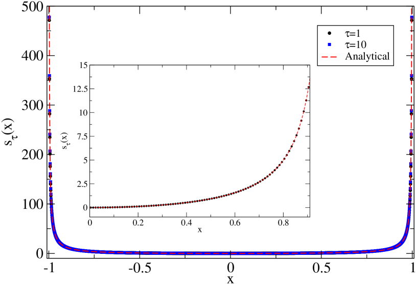
Figure 1: The function, $s_{\tau}(x)$ for to an exponential distribution of running times, $g(t)=\exp(-t/\tau)/\tau$, for $\tau=1$ (black circles) and $\tau=10$ (blue squares). The red line shows the analytical solution (30). The inset is a magnification of the central region $0<x<0.9$.

In Fig. 2 we plot the dimensionless local switching rate, $\tau\gamma_{+}(x)$, for $\tau=1$ and $\tau=10$. For both values of $\tau$, the computational results exhibit excellent agreement with the expected result that $\tau\gamma_{+}(x)=1$, up to minor discretization errors.

IV.2 Semi-Gaussian distribution

Next, we consider the case where

$$g(t)=\frac{2}{\pi\tau}\exp\left[-\frac{1}{\pi}\left(t/\tau\right)^{2}\right]\,.$$ (31)

Setting $\tau=1$ and $\tau=10$ as in section IV.1, and defining the function $s_{\tau}(x)$ as in Eq. (28), we present in Fig. 3 the results for $s_{\tau}(x)$. The shape of the curves are quite similar to the shape of the $s_{\tau}(x)$ in Fig. 1, i.e., grow moderately for $|x|\lesssim 0.9$ and exhibit a steep incline when approaching the edge of the support. However, in the present case, the (exact) $s_{\tau}(x)$ does depend on $\tau$. In the inset on Fig. 3, we see a magnification of the central region, including also results for $\tau=0.1$ that are plotted with red triangles and deviate only weakly from the data for $\tau=1$ (black circles). We note that for $\tau=0.1$, the SSD becomes so small close to the edge of the support, that it could not be computed beyond the range $|x|<0.95$ with double precision floating point.

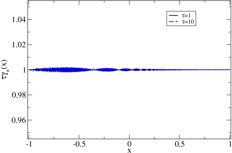
Figure 2: The dimensionless local switching rate, $\tau\gamma_{+}(x)$ corresponding to an exponential distribution of running times, for $\tau=1$ (black solid line) and $\tau=10$ (blue dashed line).

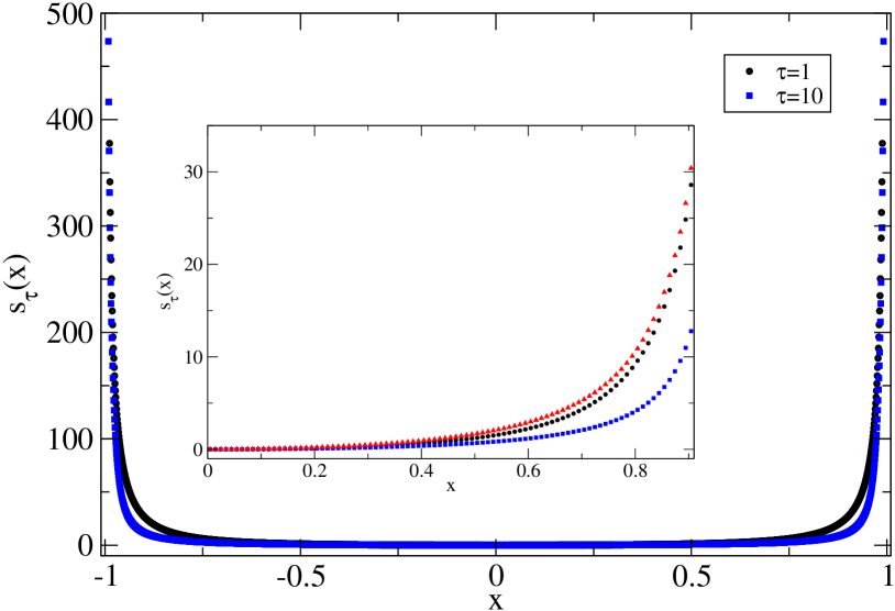
Figure 3: The function $s_{\tau}(x)$ corresponding to a semi-Gaussian distribution of running times [Eq. (31)] for $\tau=1$ (black circles) and $\tau=10$ (blue squares). The inset is a magnification of the central region $0<x<0.9$, with data also corresponding to $\tau=0.1$ which is plotted with red triangles.

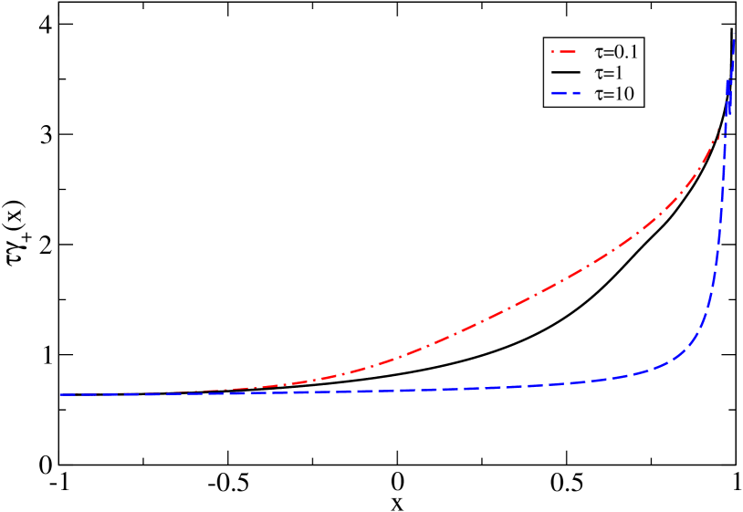
Figure 4: The dimensionless local switching rate, $\tau\gamma_{+}(x)$ corresponding to a semi-Gaussian distribution of running times, for $\tau=0.1$ (dashed-dotted red line), $\tau=1$ (black solid line), and $\tau=10$ (blue dashed line).

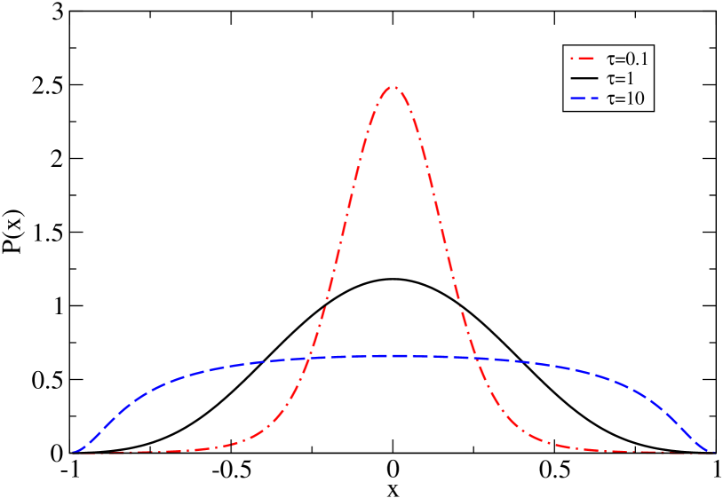
Figure 5: The SSD, $P(x)$, corresponding to a half-t distribution of running times [Eq. (36)], for $\tau=0.1$ (dashed-dotted red line), $\tau=1$ (black solid line), and $\tau=10$ (blue dashed line).

In Fig. 4 we plot the dimensionless local switching rate, $\tau\gamma_{+}(x)$, for $\tau=0.1$, $\tau=1$, and $\tau=10$. As expected, the switching rate is not constant and, moreover, depends also on $\tau$. We do, however, observe that all three curves are monotonically increasing and approach the same values on the left and right ends of the interval. These limits can be understood by noting that the switching rate can be formally written as

$$\gamma_{+}(x)=\left\langle\frac{g(t)}{1-G(t)}\right\rangle_{t=t_{+}(y\leq x,x)},$$ (32)

where the average, with the proper weights, is taken over all possible trajectories leading directly to point $x$ from a point $y\leq x$, and $t_{+}(y,x)$ is the travel time between the points [see Eq. (14)]. Close to the left end of the support ($x\rightarrow-1$), most of the trajectories are short, and the travel times $t_{+}(y,x)\ll\tau$; therefore

$$\gamma_{+}(x\rightarrow-1)\rightarrow g(0).$$ (33)

In the present case this yields $\tau\gamma_{+}(x\rightarrow-1)\rightarrow 2/\pi\simeq 0.637$, in excellent agreement with the numerical data. On the right end of the support ($x\rightarrow 1$), the different curves seem to approach the limit $\tau\gamma_{+}(x\rightarrow 1)\rightarrow 4$. This limit can be related to the asymptotic behavior of $s_{\tau}(x)$ near the edge of the support, which becomes independent of $\tau$ because of the divergence of the travel times in this region (i.e., the diminishing of the velocity). Explicitly, for $x\rightarrow 1$, Eq. (7) is well approximated by

$$\frac{d\ln[I(x)]}{dx}\simeq-\frac{\gamma_{+}(x)}{v_{+}(x)}=\frac{\mu\gamma_{+}(x)}{\sigma_{0}+F(x)}.$$ (34)

For the force function (26) with $\sigma_{0}=1$, we obtain from Eqs. (29) and (34) that

$$\frac{s_{\tau}(x\rightarrow 1)}{\tau} \simeq \frac{2\gamma_{+}(x\rightarrow 1)\mu}{\pi}\tan\left[\frac{\pi}{4}\left(1+x\right)\right]$$ (35)

$$\simeq \frac{8\gamma_{+}(x\rightarrow 1)\mu}{\pi^{2}}\frac{1}{1-x}.$$

This result applies to any function $g(t)$ (for the force function considered herein), as long as $\gamma_{+}(x)$ does not vanish when $x\rightarrow 1$ (as in the example discussed in the following subsection). In particular, it implies that $\tau\gamma_{+}(x\to 1)$ is independent of $\tau$, in agreement with our numerical results and consistent with the large-deviation principle. It is easy to check that the LDF (30) of the exponential distribution function [in which case $\gamma_{+}(x)=1/\tau$], has the same asymptotic form as the general Eq. (35).

IV.3 Half-t distribution

Consider the distribution function of running times

$$g(t)=\frac{1}{\tau}\left[1+(t/\tau)^{2}\right]^{-3/2},$$ (36)

which is a special case of the algebraically decaying half-t distribution with average running time equal to $\tau$ and diverging higher moments. Fig. 5 shows the SSDs (which have been normalized to unity) for $\tau=0.1$, $\tau=1$, and $\tau=10$. Since the distribution function $g(t)$ is fat-tailed, it is not surprising to find that the SSD is rather flat for $\tau=10$. For $\tau=1$ and $\tau=0.1$, the SSD adopts a bell-shape, but one which is far less narrowly peaked compared to the SSDs corresponding to the exponential distribution (subsection IV.1) with similar $\tau$. This is the reason why, in this case, we do not plot the functions $s_{\tau}(x)$. In fact, it is not clear whether the large-deviation principle applies here, as can be understood from Fig. 6 where we plot the dimensionless switching rate for the different values of $\tau$. All three curves approach the limit $\tau\gamma_{+}(x)\rightarrow 1$ for $x\rightarrow-1$, which is consistent with Eq. (33). On the other end of the interval, we see that all three curves converge to the limit $\tau\gamma_{+}(x\rightarrow 1)\rightarrow 0$. As noted above, the general asymptotic form (35) does not hold in such cases. The vanishing of $\gamma_{+}(x)$ close to the right edge of the support means that the stopping probability of the particle does not assume a local exponential form, see Eq. (25), which is required for the SSD to take the form $P(x)\sim\exp[-s(x)/\tau]$ in the large-deviation regime.

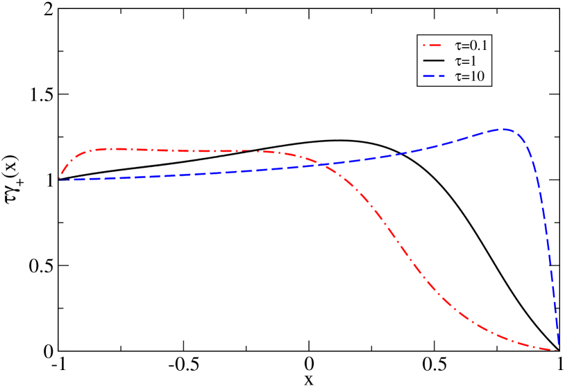
Figure 6: The dimensionless local switching rate, $\tau\gamma_{+}(x)$ corresponding to a half-t distribution of running times, for $\tau=0.1$ (dashed-dotted red line), $\tau=1$ (black solid line), and $\tau=10$ (blue dashed line).

V Discussion

To summarize, we have developed a numerical method for computing the SSD of a non-Markovian RTP, characterized by a waiting time distribution $g(t)$ between tumbling events, and trapped by an external potential in 1D. Our method succeeds in obtaining numerical results even in regions of space for which the SSD is extremely small, i.e., representing very rare events. These events are associated with situations in which the RTP is close to the edges of the SSD’s support, and they become rarer as the mean time between tumbles $\tau$ is decreased. Our method does not involve generating (naive or biased) realizations of the RTP’s dynamics. Instead, it is based on an analytical derivation that leads to a set of integral equations whose solution yields the SSD. We essentially solve these integral equations numerically.

To illustrate our method, we applied it to three different distributions $g(t)$: (i) Exponential, (ii) semi-Gaussian, and (iii) half-t. In the first example, one recovers the standard (Markovian) RTP, whose SSD is known exactly. This case serves as a useful benchmark for our method. The last example leads to very different scaling behaviors since $g(t)$ is fat tailed.

The computation of the SSD and the function $s_{\tau}(x)$ that is closely related to it, also enables us to compute the LDF, $s(x)$. This is done by combining results for different values of $\tau$, and considering the asymptotic behavior of $s_{\tau}(x)$ in the limit $\tau\rightarrow 0$. Near the edge of the SSD’s support, the LDF is characterized by (i) a diverging function, and (ii) the asymptotic value of the position-dependent tumbling rate $\gamma_{+}(x)$. These depend on the form of the external force, $F(x)$, and on the distribution function of the waiting times, $g(t)$ [under mild assumptions regarding $g(t)$], but not on $\tau$. For the specific external force (26), we obtained analytically that $s(x)$ diverges as a power law. This particular behavior appears to be related to a special property of the force (26): Its derivative, $F^{\prime}(x)$, vanishes at the edge. In the more generic case in which this does not occur, other behaviors are to be expected (e.g., logarithmic divergence SmithFarago22 ). Note that $s(x)$ is an extremely useful object. Given $s(x)$ for a specific potential, one can immediately compute from it the rate function, $\Phi(z)$ (see definition in SmithFarago22 ; Smith2023 ) that describes dynamical fluctuations of the RTP’s position in the absence of external forces. From the knowledge of $\Phi(z)$, one can then work in the opposite route and obtain $s(x)$ for other potentials Smith2023 .

Our method (perhaps with minor adjustments) may be applicable to non-confining potentials as well, and could therefore prove useful to study escape or first-passage statistics, or behavior within periodic potentials, for non-Markovian RTPs. It would be also interesting to extend our method to more general settings, e.g., to higher dimensions or to other possible non-Markovian active models (e.g., one could consider non-Markovian versions of the active Brownian particle).

Acknowledgments

We acknowledge support from the Israel Science Foundation (ISF) through Grants No. 1258/22 (OF) and 2651/23 (NRS).

References

- (1) F. Schweitzer, Brownian Agents and Active Particles: Collective Dynamics in the Natural and Social Sciences, Springer: Complexity, Berlin, (2003).
- (2) P. Romanczuk, M. Bär, W. Ebeling, B. Lindner, and L. Schimansky-Geier, Active Brownian particles, Eur. Phys. J. Special Topics 202, 1 (2012).
- (3) M. C. Marchetti, J. F. Joanny, S. Ramaswamy, T. B. Liverpool, J. Prost, M. Rao, and R. Aditi Simha, Hydrodynamics of soft active matter, Rev. Mod. Phys. 85, 1143 (2013).
- (4) É. Fodor, M. Guo, N. Gov, P. Visco, D. Weitz, and F. van Wijland, Activity-driven fluctuations in living cells, Europhys. Lett. 110, 48005 (2015).
- (5) É. Fodor, C. Nardini, M. E. Cates, J. Tailleur, P. Visco, and F. van Wijland, How Far from Equilibrium Is Active Matter?, Phys. Rev. Lett. 117, 038103 (2016).
- (6) C. Bechinger, R. Di Leonardo, H. Löwen, C. Reichhardt, G. Volpe, and G. Volpe, Active particles in complex and crowded environments, Rev. Mod. Phys. 88, 045006 (2016).
- (7) S. Ramaswamy, Active matter, J. Stat. Mech. 054002 (2017).
- (8) D. Needleman and Z. Dogic, Active matter at the interface between materials science and cell biology, Nat. Rev. Mater. 2, 17048 (2017).
- (9) É. Fodor, and M. C. Marchetti, The statistical physics of active matter: from self-catalytic colloids to living cells, Physica A 504, 106 (2018).
- (10) É. Fodor, R. L. Jack and M. E. Cates, Irreversibility and Biased Ensembles in Active Matter: Insights from Stochastic Thermodynamics, Annu. Rev. Condens. Matter Phys. 13, 215 (2022).
- (11) F. Backouche, L. Haviv, D. Groswasser, and A. Bernheim-Groswasser, Active gels: dynamics of patterning and self-organization, Phys. Biol. 3, 264 (2006).
- (12) D. Mizuno, C. Tardin, C. F. Schmidt, and F. C. MacKintosh, Nonequilibrium Mechanics of Active Cytoskeletal Networks, Science 315, 370 (2007).
- (13) T. Toyota, D. A. Head, C. F. Schmidt, and D. Mizuno, Non-Gaussian athermal fluctuations in active gels, Soft Matter 7, 3234 (2011).
- (14) B. Stuhrmann, M. S. e Silva, M. Depken, F. C. MacKintosh and G. H. Koenderink, Nonequilibrium fluctuations of a remodeling in vitro cytoskeleton, Phys. Rev. E 86, 020901(R) (2012).
- (15) E. Coli in Motion, H. C. Berg, (Springer Verlag, Heidelberg, Germany) (2004).
- (16) C. Wilhelm, Out-of-Equilibrium Microrheology inside Living Cells, Phys. Rev. Lett. 101, 028101 (2008)
- (17) M. E. Cates, Diffusive transport without detailed balance: Does microbiology need statistical physics?, Rep. Prog. Phys. 75, 042601 (2012).
- (18) W. W. Ahmed, E. Fodor, M. Almonacid, M. Bussonnier, M.-H. Verlhac, N. S. Gov, P. Visco, F. van Wijland, and T. Betz, Active cell mechanics: Measurement and theory, Biochim. Biophys. Acta 1853, 3083 (2015).
- (19) A. Be’er, B. Ilkanaiv, R. Gross, D. B. Kearns, S. Heidenreich, M. Bär and G. Ariel , A phase diagram for bacterial swarming, Commun. Phys. 3, 66 (2020).
- (20) D. Breoni, F. J. Schwarzendahl, R. Blossey, H. Löwen, A one-dimensional three-state run-and-tumble model with a ‘cell cycle’, Eur. Phys. J. E 45, 83 (2022).
- (21) D. Nishiguchi, Deciphering long-range order in active matter: Insights from swimming bacteria in quasi-2D and electrokinetic Janus particles, arXiv:2306.17689.
- (22) J. Toner, Y. Tu, and S. Ramaswamy, Hydrodynamics and phases of flocks, Ann. of Phys. 318, 170 (2005).
- (23) N. Kumar, H. Soni, S. Ramaswamy, and A. K. Sood, Flocking at a distance in active granular matter, Nature Comm. 5, 4688 (2014).
- (24) T. Vicsek, A. Czirók, E. Ben-Jacob, I. Cohen, and O. Shochet, Novel Type of Phase Transition in a System of Self-Driven Particles, Phys. Rev. Lett. 75, 1226 (1995).
- (25) S. Hubbard, P. Babak, S. Th. Sigurdsson, and K. G. Magnússon, A model of the formation of fish schools and migrations of fish, Ecol. Modell. 174, 359 (2004).
- (26) R. Golestanian, T. B. Liverpool, and A. Ajdari, Designing phoretic micro-and nano-swimmers, New J. Phys. 9, 126 (2007).
- (27) B. ten Hagen, F. Kümmel, R. Wittkowski, D. Takagi, H. Löwen and C. Bechinger, Gravitaxis of asymmetric self-propelled colloidal particles, Nature Comm. 5, 4829 (2014).
- (28) S. C. Takatori, R. De Dier, J. Vermant, and J. F. Brady, Acoustic trapping of active matter, Nat. Commun. 7, 10694 (2016).
- (29) L. Walsh, C. G. Wagner, S. Schlossberg, C. Olson, A. Baskaran, and N. Menon, Noise and diffusion of a vibrated self-propelled granular particle, Soft Matter 13, 8964 (2017).
- (30) A. Deblais, T. Barois, T. Guerin, P.H. Delville, R. Vaudaine, J. S. Lintuvuori, J. F. Boudet, J. C. Baret, and H. Kellay, Boundaries Control Collective Dynamics of Inertial Self-Propelled Robots, Phys. Rev. Lett. 120, 188002 (2018).
- (31) O. Dauchot and V. Démery, Dynamics of a Self-Propelled Particle in a Harmonic Trap, Phys. Rev. Lett. 122, 068002 (2019).
- (32) A. Poncet, O. Bénichou, V. Démery, and D. Nishiguchi, Pair correlation of dilute active Brownian particles: From low-activity dipolar correction to high-activity algebraic depletion wings, Phys. Rev. E 103, 012605 (2021).
- (33) I. Buttinoni, L. Caprini, L. Alvarez, F. J. Schwarzendahl, H. Löwen, Active colloids in harmonic optical potentials, Europhys. Lett. 140, 27001 (2022).
- (34) A. A. Molodtsova, M. K. Buzakov, A. D. Rozenblit, V. A. Smirnov, D. V. Sennikova, V. A. Porvatov, O. I. Burmistrov, E. M. Puhtina, A. A. Dmitriev, N. A. Olekhno, Experimental demonstration of robotic active matter micellization, arXiv:2305.16659.
- (35) S. Paramanick, A. Pal, H. Soni, N. Kumar, Programming tunable active dynamics in a self-propelled robot, arXiv:2306.06609
- (36) J. Schwarz-Linek, C. Valeriani, A. Cacciuto, M. E. Cates, D. Marenduzzo, A. N. Morozov, and W. C. K. Poon, Phase separation and rotor self-assembly in active particle suspensions, Proc. Natl. Acad. Sci. USA 109, 4052 (2012).
- (37) G. S. Redner, M. F. Hagan, and A. Baskaran, Structure and Dynamics of a Phase-Separating Active Colloidal Fluid, Phys. Rev. Lett. 110, 055701 (2013).
- (38) J. Stenhammar, R. Wittkowski, D. Marenduzzo, and M. E. Cates, Activity-Induced Phase Separation and Self-Assembly in Mixtures of Active and Passive Particles, Phys. Rev. Lett. 114, 018301 (2015).
- (39) Y. Fily, and M. C. Marchetti, Athermal Phase Separation of Self-Propelled Particles with No Alignment, Phys. Rev. Lett. 108, 235702 (2012).
- (40) J. Palacci, S. Sacanna, A. P. Steinberg, D. J. Pine, and P. M. Chaikin, Living crystals of light-activated colloidal surfers, Science 339, 936 (2013).
- (41) A. B. Slowman, M. R. Evans, and R. A. Blythe, Jamming and Attraction of Interacting Run-and-Tumble Random Walkers, Phys. Rev. Lett. 116, 218101 (2016).
- (42) A. P. Solon, Y. Fily, A. Baskaran, M. E. Cates, Y. Kafri, M. Kardar, J. Tailleur, Pressure is not a state function for generic active fluids, Nature Phys. 11, 673 (2015).
- (43) S. Put, J. Berx and C. Vanderzande, Non-Gaussian anomalous dynamics in systems of interacting run-and-tumble particles, J. Stat. Mech. (2019) 123205.
- (44) P. Singh, A. Kundu, Crossover behaviours exhibited by fluctuations and correlations in a chain of active particles, J. Phys. A: Math. Theor. 54, 305001 (2021).
- (45) T. Agranov, S. Ro, Y. Kafri, and V. Lecomte, Exact fluctuating hydrodynamics of active lattice gases – typical fluctuations, J. Stat. Mech (2021), 083208.
- (46) T. Banerjee, R. L. Jack and M. E. Cates, Tracer dynamics in one dimensional gases of active or passive particles, J. Stat. Mech. (2022) 013209.
- (47) T. Agranov, S. Ro, Y. Kafri, and V. Lecomte, Macroscopic Fluctuation Theory and current fluctuations in active lattice gases, SciPost Phys. 14, 045 (2023).
- (48) R. Sarkar, I. Santra, U. Basu, Stationary states of activity driven harmonic chains, Phys. Rev. E 107, 014123 (2023).
- (49) T. Agranov, M. E. Cates and R. L. Jack, Entropy production and its large deviations in an active lattice gas, J. Stat. Mech. (2022) 123201.
- (50) H. H. Wensink and H. Löwen, Aggregation of self-propelled colloidal rods near confining walls, Phys. Rev. E 78, 031409 (2008).
- (51) P. Singh and A. Kundu, Generalised ‘Arcsine’ laws for run-and-tumble particle in one dimension, J. Stat. Mech. 083205 (2019).
- (52) N. R. Smith., P. Le Doussal., S. N. Majumdar, G. Schehr, Exact position distribution of a harmonically-confined run-and-tumble particle in two dimensions, Phys. Rev. E 106, 054133 (2022).
- (53) N. R. Smith, Nonequilibrium steady state of trapped active particles, Phys. Rev. E 108, L022602 (2023).
- (54) D. Frydel, Active oscillator: recurrence relation approach, arXiv:2312.05406
- (55) N. R. Smith and O. Farago, Nonequilibirum steady state for harmonically-confined active particles, Phys. Rev. E 106, 054118 (2022).
- (56) J. Tailleur, M. E. Cates, Statistical Mechanics of Interacting Run-and-Tumble Bacteria, Phys. Rev. Lett. 100, 218103 (2008); Sedimentation, trapping, and rectification of dilute bacteria, Europhys. Lett. 86, 60002 (2009).
- (57) J. Elgeti and G. Gompper, Self-propelled rods near surfaces, Europhys. Lett. 85, 38002 (2009).
- (58) Guanglai Li and Jay X. Tang, Accumulation of Microswimmers near a Surface Mediated by Collision and Rotational Brownian Motion, Phys. Rev. Lett. 103, 078101 (2009).
- (59) A. Kaiser, H. H. Wensink, and H. Löwen, How to Capture Active Particles, Phys. Rev. Lett. 108, 268307 (2012).
- (60) A. Pototsky, and H. Stark, Active Brownian particles in two-dimensional traps, Europhys. Lett. 98, 50004 (2012).
- (61) J. Elgeti and G. Gompper. Wall accumulation of self-propelled spheres, Europhys. Lett. 101, 48003 (2013).
- (62) M. Hennes, K. Wolff, and H. Stark, Self-Induced Polar Order of Active Brownian Particles in a Harmonic Trap, Phys. Rev. Lett. 112, 238104 (2014).
- (63) A. P. Solon, M. E. Cates, and J. Tailleur, Active brownian particles and run-and-tumble particles: A comparative study, Eur. Phys. J. Special Topics 224, 1231 (2015).
- (64) Y. Li, F. Marchesoni, T. Debnath, and P. K. Ghosh, Two-dimensional dynamics of a trapped active Brownian particle in a shear flow, Phys. Rev. E 96, 062138, (2017).
- (65) N. Razin, R. Voituriez, J. Elgeti, and N. S. Gov, Forces in inhomogeneous open active-particle systems, Phys. Rev. E 96, 052409, (2017).
- (66) C. Kurzthaler, S. Leitmann, T. Franosch, Intermediate scattering function of an anisotropic active Brownian particle, Sci. Rep. 6, 36702 (2016).
- (67) S. Das, G. Gompper, and R. G. Winkler, Confined active Brownian particles: theoretical description of propulsion-induced accumulation, New J. Phys. 20, 015001 (2018).
- (68) L. Caprini and U. M. B. Marconi, Active chiral particles under confinement: surface currents and bulk accumulation phenomena, Soft Matter 15, 2627 (2019).
- (69) F. J. Sevilla, A. V. Arzola, and E. P. Cital, Stationary superstatistics distributions of trapped run-and-tumble particles, Phys. Rev. E 99, 012145 (2019).
- (70) U. Basu, S. N. Majumdar, A. Rosso, G. Schehr, Long time position distribution of an active Brownian particle in two dimensions, Phys. Rev. E 100, 062116 (2019).
- (71) A. Dhar, A. Kundu, S. N. Majumdar, S. Sabhapandit, G. Schehr, Run-and-Tumble particle in one-dimensional confining potential: Steady state,relaxation and first passage properties, Phys. Rev. E 99, 032132 (2019).
- (72) K. Malakar, A. Das, A. Kundu, K. Vijay Kumar, A. Dhar, Steady state of an active Brownian particle in a two-dimensional harmonic trap, Phys. Rev. E 101, 022610 (2020).
- (73) I. Santra, U. Basu, S. Sabhapandit, Direction reversing active Brownian particle in a harmonic potential, Soft Matter 17, 10108 (2021).
- (74) K. Malakar, V. Jemseena, A. Kundu, K. Vijay Kumar, S. Sabhapandit, S. N. Majumdar, S. Redner and A. Dhar, Steady state, relaxation and first-passage properties of a run-and-tumble particle in one-dimension, J. Stat. Mech. (2018) 043215.
- (75) U. Basu, S. N. Majumdar, A. Rosso, G. Schehr, Active Brownian Motion in Two Dimensions, Phys. Rev. E 98, 062121 (2018).
- (76) D. Boyer, S. N. Majumdar, An active particle in one dimension subjected to resetting with memory, arXiv:2312.13439
- (77) P. Le Doussal, S. N. Majumdar, and G. Schehr, Velocity and diffusion constant of an active particle in a one-dimensional force field, Europhys. Lett. 130, 40002 (2020).
- (78) G. H. Weiss, Some applications of persistent random walks and the telegrapher’s equation, Physica A, 311, 381 (2002).
- (79) S. Herrmann and P. Vallois, From persistent random walks to the telegraph noise, Stoch. Dyn. 10, 161 (2010).
- (80) H. G. Othmer, S. R. Dunbar, and W. Alt, Models of dispersal in biological systems, J. Math. Biol. 26, 263 (1988).
- (81) K. Martens, L. Angelani, R. Di Leonardo, and L. Bocquet, Probability distributions for the run-and-tumble bacterial dynamics: An analogy to the Lorentz model, Eur. Phys. J E 35, 84 (2012).
- (82) M. R. Evans and S. N. Majumdar, Run and tumble particle under resetting: a renewal approach, J. Phys. A: Math. Theor. 51, 475003 (2018).
- (83) I. Santra, U. Basu and S. Sabhapandit, Run-and-tumble particles in two dimensions: Marginal position distributions, Phys. Rev. E 101, 062120 (2020).
- (84) D. S. Dean, S. N. Majumdar, and H. Schawe, Position distribution in a generalized run-and-tumble process, Phys. Rev. E 103, 012130 (2021).
- (85) D. Frydel, Positing the problem of stationary distributions of active particles as third-order differential equation, Phys. Rev. E 106, 024121 (2022).
- (86) F. Cinque, E. Orsingher, Stochastic dynamics of generalized planar random motions with orthogonal directions, J. Theor. Prob. 36, 2229 (2023).
- (87) S. N. Majumdar and B. Meerson, Toward the full short-time statistics of an active Brownian particle on the plane, Phys. Rev. E 102, 022113 (2020).
- (88) S. N. Majumdar and G. Schehr, Large Deviations, ICTS Newsletter 2017 (Volume 3, Issue 2).
- (89) A. Dembo and O. Zeitouni, Large Deviations Techniques and Applications, 2nd ed. (Springer, New York, 1998).
- (90) F. den Hollander, Large Deviations, Fields Institute Monographs, vol. 14 (AMS, Providence, Rhode Island, 2000).
- (91) S. N. Majumdar, Brownian Functionals in Physics and Computer Science, Current Science, vol-89, 2076 (2005).
- (92) H. Touchette, The large deviation approach to statistical mechanics, Phys. Rep. 478, 1 (2009).
- (93) B. Derrida, Microscopic versus macroscopic approaches to non-equilibrium systems, J. Stat. Mech. P01030 (2011).
- (94) H. Touchette, Introduction to dynamical large deviations of Markov processes, Physica A 504, 5 (2018).
- (95) Note that often in the literature the standard RTP is referred to as a non-Markovian model too, the interpretation being that its future dynamics do not depend on its instantaneous position alone.
- (96) W. Wang, E. Barkai and S. Burov, Large Deviations for Continuous Time Random Walks, Entropy 22, 697 (2020).
- (97) R. K. Singh and S. Burov, Universal to nonuniversal transition of the statistics of rare events during the spread of random walks, Phys. Rev. E 108, L052102 (2023).
- (98) A. K. Hartmann, Sampling rare events: Statistics of local sequence alignments, Phys. Rev. E 65, 056102 (2002).
- (99) J. Tailleur and V. Lecomte, Simulation of large deviation functions using population dynamics, AIP Conf. Proc. 1091, 212 (2009).
- (100) P. I. Hurtado and P. L. Garrido, Spontaneous Symmetry Breaking at the Fluctuating Level, Phys. Rev. Lett. 107, 180601 (2011).
- (101) H. Touchette, A basic introduction to large deviations: Theory, applications, simulations, in: R. Leidl, A. K. Hartmann (Eds.), Modern Computational Science 11: Lecture Notes from the 3rd International Oldenburg Summer School, BIS-Verlag der Carl von Ossietzky Universität Oldenburg, (2011), arXiv:1106.4146.
- (102) G. Claussen, A. K. Hartmann, and S. N. Majumdar, Convex hulls of random walks: Large-deviation properties, Phys. Rev. E 91, 052104 (2015).
- (103) A. K. Hartmann, P. Le Doussal, S. N. Majumdar, A. Rosso, and G. Schehr, High-precision simulation of the height distribution for the KPZ equation, Europhys. Lett. 121, 67004 (2018).
- (104) T. Grafke and E. Vanden-Eijnden, Numerical computation of rare events via large deviation theory, Chaos 29, 063118 (2019).
- (105) J. Börjes, H. Schawe, A. K. Hartmann, Large deviations of the length of the longest increasing subsequence of random permutations and random walks, Phys. Rev. E 99, 042104 (2019).
- (106) A. K. Hartmann, B. Meerson, P. Sasorov, Optimal paths of nonequilibrium stochastic fields: The Kardar-Parisi-Zhang interface as a test case, Phys. Rev. Res. 1, 032043 (2019).
- (107) A. K. Hartmann, S. N. Majumdar, H. Schawe, and G. Schehr, The convex hull of the run-and-tumble particle in a plane, J. Stat. Mech. 053401 (2020).
- (108) A. K. Hartmann, B. Meerson, P. Sasorov, Observing symmetry-broken optimal paths of stationary Kardar-Parisi-Zhang interface via a large-deviation sampling of directed polymers in random media, Phys. Rev. E 104, 054125 (2021).
- (109) D. Nickelsen and H. Touchette, Noise correction of large deviations with anomalous scaling, Phys. Rev. E 105, 064102 (2022).
- (110) N. R. Smith, Large deviations in chaotic systems: exact results and dynamical phase transition, Phys. Rev. E 106, L042202 (2022).
- (111) L. Causer, M. Carmen Bañuls, J. P. Garrahan, Optimal sampling of dynamical large deviations in two dimensions via tensor networks, Phys. Rev. Lett. 130, 147401 (2023)..
- (112) C. Monthus, Large deviations at various levels for run-and-tumble processes with space-dependent velocities and space-dependent switching rates, J. Stat. Mech. 2021, 083212 (2021).
- (113) W. Horsthemke and R. Lefever, Noise-Induced Transitions: Theory and applications in Physics, Chemistry and Biology, Springer-Verlag, Berlin, (1984)
- (114) V. I. Klyatskin, Radiophys. Quantum El. 20, 382 (1977).
- (115) V. I. Klyatskin, Radiofizika 20, 562 (1977).
- (116) K. Kitahara, W. Horsthemke, R. Lefever, and I. Inaba, Phase Diagrams of Noise Induced Transitions: Exact Results for a Class of External Coloured Noise, Prog. Theor. Phys. 64, 1233 (1980).
- (117) C. Van den Broeck and P. Hänggi, Activation rates for nonlinear stochastic flows driven by non-Gaussian noise, Phys. Rev. A 30, 2730 (1984).
- (118) P. Hänggi, P. Jung, Colored Noise in Dynamical Systems, Adv. Chem. Phys. 89 239, (1995).