Deep Learning Based Superposition Coded Modulation for Hierarchical Semantic Communications over Broadcast Channels

Abstract

We consider multi-user semantic communications over broadcast channels. While most existing works consider that each receiver requires either the same or independent semantic information, this paper explores the scenario where the semantic information desired by different receivers is different but correlated. In particular, we investigate semantic communications over Gaussian broadcast channels where the transmitter has a common observable source but the receivers wish to recover hierarchical semantic information in adaptation to their channel conditions. Inspired by the capacity achieving property of superposition codes, we propose a deep learning based superposition coded modulation (DeepSCM) scheme. Specifically, the hierarchical semantic information is first extracted and encoded into basic and enhanced feature vectors. A linear minimum mean square error (LMMSE) decorrelator is then developed to obtain a refinement from the enhanced features that is uncorrelated with the basic features. Finally, the basic features and their refinement are superposed for broadcasting after probabilistic modulation. Experiments are conducted for two-receiver image semantic broadcasting with coarse and fine classification as hierarchical semantic tasks. DeepSCM outperforms the benchmarking coded-modulation scheme without a superposition structure, especially with large channel disparity and high order modulation. It also approaches the performance upperbound as if there were only one receiver.

I Introduction

Semantic communication has recently emerged to deliver intelligent services. Departing from the traditional focus on source recovery, it revolutionizes data transmission by extracting and transmitting the “semantic information” crucial for the intelligent tasks at the receiver[2, 3, 4, 5]. Therefore, semantic communications can significantly improve transmission efficiency and service quality over traditional Shannon-type communications.

Leveraging the advantages of deep learning, semantic communication has mainly adopted neural networks (NNs) for semantic coding, which demonstrates superior performance in point-to-point communication scenarios. In particular, NN-based semantic coding has been used to substitute the conventional source coding and/or channel coding to transmit various source data types including speeches[6], texts[7, 8, 9], images[10, 11, 12, 13], videos[14, 15] as well as multi-modal data[16]. It also facilitates the execution of a wide range of intelligent semantic tasks, such as object detection[17], classification[10], and question-answering[16]. Different types of NNs have been employed for the semantic coding of different source data types. For example, the Resnet [18] is often used for image sources[10] while the Transformer[19] is often used for the text sources. Moreover, while earlier semantic communication systems often employ analog modulation to directly transmit through the channel the real-valued output of the NN-based semantic encoder[6, 10, 7], recent advancements have brought forth digital semantic communications by taking into account digital modulation explicitly in [20, 21, 22, 23, 24]. The works [20, 21] consider codebook-based quantization methods, and the work [22] designs a learned soft-to-hard quantizer. Moreover, the works [23, 24] introduce a novel joint coding-modulation framework for end-to-end design of digital semantic communication systems, which utilizes variational autoencoder (VAE) to output the transition probability from source data to discrete constellation symbols, and can approach the optimal probabilistic constellation shaping under Gaussian channels.

TABLE I: Summary of Notation.

Notation	Description
$\mathbf{S}_{1}$, $\mathbf{\hat{S}}_{1}$	Coarse-grained semantic information and its recovery at Receiver 1
$\mathbf{S}_{2}$, $\mathbf{\hat{S}}_{2}$	Fine-grained semantic information and its recovery at Receiver 2
$\mathbf{X}$, $\mathbf{\hat{X}}_{1}$, $\mathbf{\hat{X}}_{2}$	Observable image source and its recoveries respectively at Receiver 1 and Receiver 2
$\mathbf{U}_{1}$	Basic encoded feature vector
$\mathbf{U}_{2}$	Enhanced encoded feature vector
$\mathbf{R}$	Successive refinement vector
$\mathbf{Y}_{1}$, $\mathbf{Y}_{2}$	Inner constellation sequence and outer constellation sequence
$\mathbf{Y}$	The super-constellation sequence to be sent into the channel
$\mathbf{Z}_{i}$	Received sequence of Receiver $i$
$f_{\bm{\theta}_{1}}(\cdot)$	Basic semantic encoder
$f_{\bm{\theta}_{2}}(\cdot)$	Enhancement semantic encoder
$\mathbf{W}$, $\mathbf{b}$	Weight and bias of the LMMSE decorrelator
$\bm{\alpha}_{i}$	NN parameters of Modulator $i$
$g_{\bm{\eta}_{1}}(\cdot)$, $g_{\bm{\eta}_{2}}(\cdot)$	Semantic decoders for image recovery of Receiver 1 and Receiver 2
$g_{\bm{\psi}_{1}}(\cdot)$, $g_{\bm{\psi}_{2}}(\cdot)$	Semantic decoders for coarse classification of Receiver 1 and fine classification of Receiver 2

While substantial research has been devoted to point-to-point semantic communications[6, 7, 8, 9, 10, 11, 12, 14, 15, 23], recently there is a growing interest in semantic communications over multi-user channels. Many-to-one semantic communication systems with multiple transmitters and a single receiver are considered in the works [25, 26, 27, 16, 28, 29, 30]. Specifically, the work [25] introduces a distributed joint source-channel coding (JSCC) scheme for correlated image sources, where each source is transmitted through a dedicated and independent noisy channel to the common receiver. A distributed JSCC scheme for image transmission over Gaussian multiple access channel (MAC) is considered in [26]. The work [27] considers a multi-user fading channel and introduces a channel-transferable semantic communication for orthogonal frequency division multiplexing with non-orthogonal multiple access (OFDM-NOMA) system. Moreover, works [16, 28, 29] consider multi-user channels with a multi-antenna receiver, where [28] considers cooperative object identification, while [16] and [29] address the transmission of multimodal data. Additionally, a novel multiple access technology called model division multiple access (MDMA) is proposed in [30], where both uplink and downlink scenarios are considered.

Research on semantic communications over one-to-many broadcast channels has also been conducted[31, 32, 33, 34, 35], which is aligned with the focus of this paper. Specifically, the work [31] introduces a feature-disentangled semantic broadcasting communication system. Therein, the extracted receiver-specific semantic features from a common source are encoded using conventional bit-level source and channel coding. The work [32] proposes an image semantic fusion scheme that combines the semantic features for different receivers into a unified latent representation before broadcasting. The work [33] introduces a downlink NOMA-enhanced semantic communication system with diverse modalities of sources. Therein, the semantic features of different users are mapped into discrete constellations via an asymmetric quantizer and then superposed for broadcasting. Moreover, to better deal with diverse channel conditions among multiple receivers, the authors in [34] propose to first jointly train the transmitter with one receiver, then employ transfer learning for the other receiver. The work [35] proposes a reinforcement learning based self-critical alternate learning algorithm for adapting to different channel conditions with sentence generation task. Notably, these existing research efforts largely focus on the scenarios where the multiple receivers either require independent semantic information[31, 32, 33] or desire the common semantics[34, 35]. It remains unexplored the scenarios where the required semantic information by different receivers is different but correlated.

In this paper we investigate semantic communication over a two-user broadcast channel where the different but correlated semantic information needed by the two receivers exhibits a hierarchical structure. Specifically, the common observable source and the associated semantic information are modeled as a hierarchical structure. The receiver with poor channel condition wishes to recover the observable source and the coarse-grained semantic information while the receiver with good channel condition wishes to recover the observable source and the fine-grained semantic information. Our goal is to design an efficient digital semantic communication framework that can exploit such hierarchical structure of semantic information and accommodate the diverse channel conditions of different receivers.

To this end, we propose a novel deep learning-based superposition coded modulation (DeepSCM) scheme for hierarchical semantic communications over Gaussian degraded broadcast channels. Inspired by the capacity achieving property of superposition codes for degraded broadcast channels[36], our DeepSCM scheme is able to extract uncorrelated features for different receivers from a common observable source and encode them into a superposition-structured constellation, so that each receiver can decode different levels of semantic information according to its own channel condition. Specifically, we first use two separate NN-based semantic encoders to encode the common observable source into a basic encoded feature vector for the poor receiver and an enhanced encoded feature vector for the good receiver respectively. Recognizing the existing correlation between them, we thus design a decorrelator. This decorrelator splits the enhanced encoded feature vector into two parts, one containing information highly correlated with the basic encoded feature vector, the other containing uncorrelated information. The latter is denoted as the successive refinement vector of the basic encoded feature vector, and is subsequently modulated for transmission. Moreover, we design a modulation strategy, associating the basic encoded feature vector with the inner layer of a superposition-structured constellation and the successive refinement vector with the outer layer. As a result, the poor receiver can successfully decode the inner layer and recover the first level of semantic information. At the same time, the good receiver can further decode the outer layer, therefore recovering the enhanced level of semantic information.

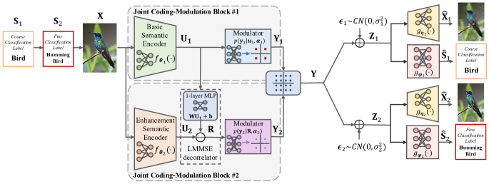
Figure 1: The framework of the proposed DeepSCM scheme.

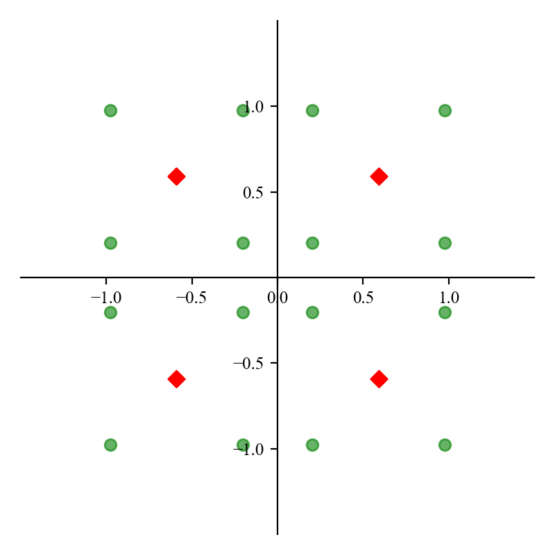
(a) 4QAM$\times$4QAM, $a=0.7$.

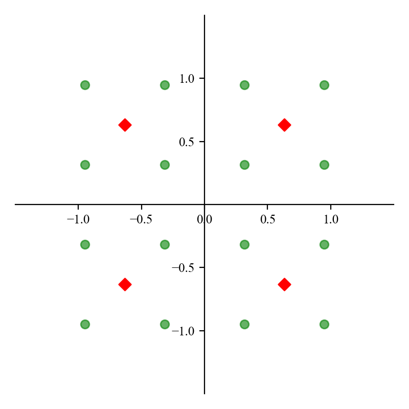
(b) 4QAM$\times$4QAM, $a=0.8$.

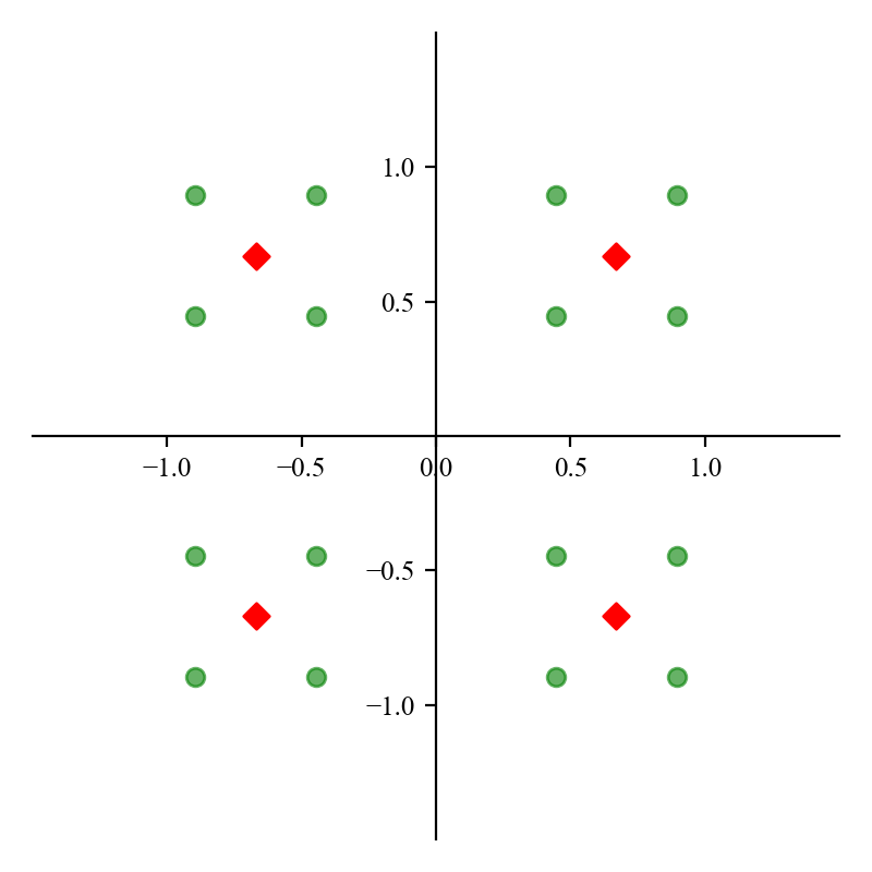
(c) 4QAM$\times$4QAM, $a=0.9$.

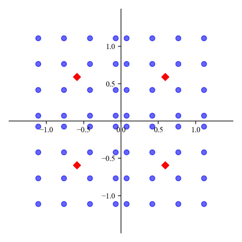
(d) 4QAM$\times$16QAM, $a=0.7$.

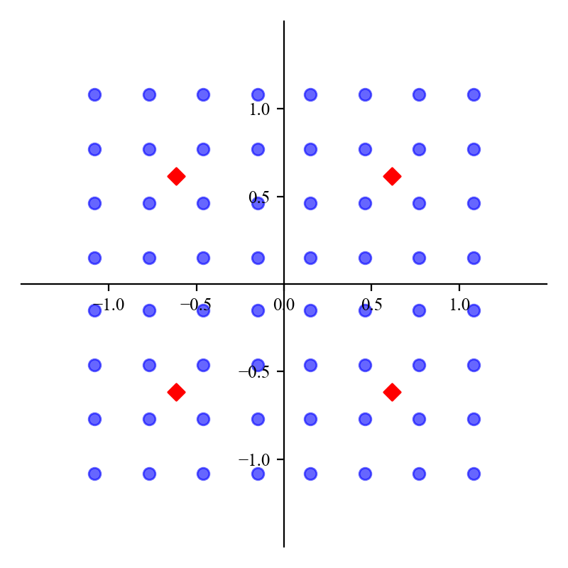
(e) 4QAM$\times$16QAM, $a=0.76$.

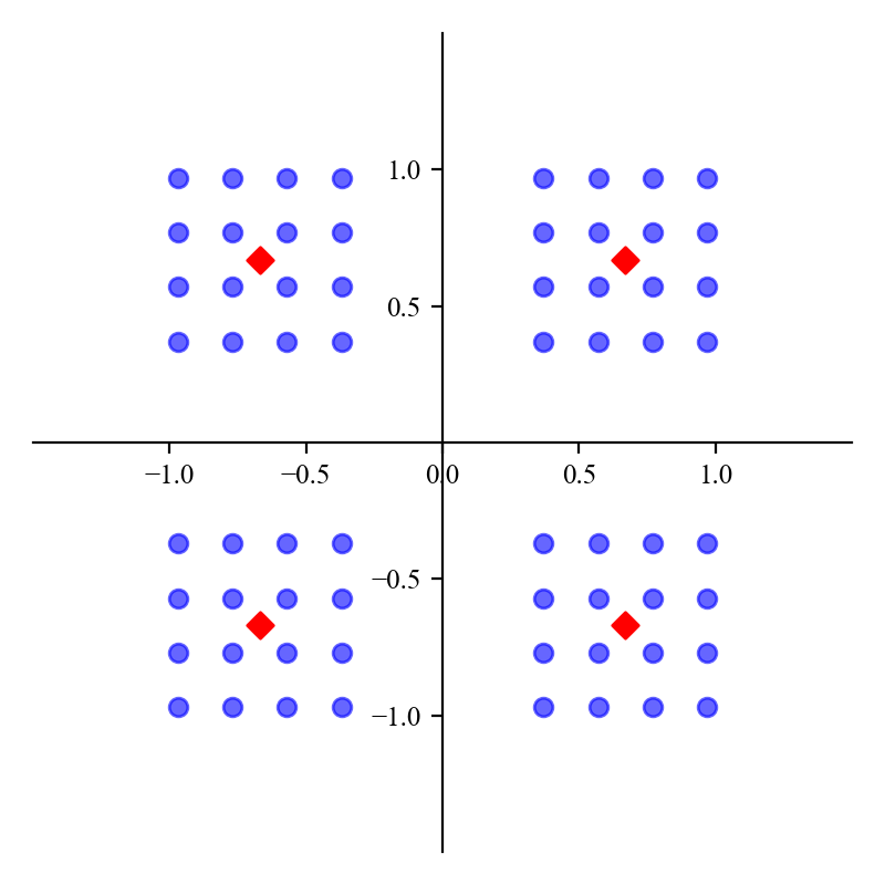
(f) 4QAM$\times$16QAM, $a=0.9$.

Figure 2: Constellations after superposition with various values of $a$. The red diamonds indicate the inner constellation multiplied by the PAF, and the dots indicate the resulted super-constellation. All symbols are assumed to be uniformly distributed in this figure with $P=1$. Notably, (b) and (e) present rectangular 16QAM and 64QAM, respectively.

Our main contribution is to propose a novel NN-based architecture for hierarchical semantic communications, namely the DeepSCM scheme, according to the idea presented above. Our proposed scheme combines the benefits of NN-based coding and the classical superposition coding to enable efficient semantic communications over Gaussian degraded broadcast channels. To implement such a complex system, the following efforts have been made. First, to improve transmission efficiency, we design a novel module called the linear mininum mean square error (LMMSE) decorrelator to decorrelate the enhanced encoded feature vector with the basic encoded feature vector, obtaining the successive refinement vector of the basic encoded feature vector. Theoretical proof is further provided to establish that the successive refinement vector and the basic encoded feature vector can indeed be uncorrelated through optimization. Second, to ensure the convergence and the performance of the training process, we devise a three-stage training strategy for the training of the DeepSCM scheme according to the superposition structure. Extensive experiments on real-world datasets validate two performance advantages of our DeepSCM scheme. First, our proposed DeepSCM scheme can simultaneously approach the best achievable performances for both receivers, as if there were only one receiver. Second, it outperforms the coded modulation scheme without superposition structure, where the transmitter only uses a single semantic encoder that is trained jointly with the semantic decoders at the two receivers. This performance advantage grows as the channel signal-to-noise (SNR) gap between the two receivers widens and the modulation order increases.

The rest of the paper is organized as follows. The overall framework of DeepSCM is presented in Section II. Section III describes the transmitter design in detail, including the main components of the transmitter and the training strategy. In Section IV, we evaluate the performance of our proposed DeepSCM scheme through extensive experiments. Finally, we conclude the paper in Section V.

Throughout this paper, we use upper-case letters ($X$) and lower-case letters ($x$) to respectively denote random variables and their realizations. We use $h(X)$ to denote the differential entropy of the continuous variable $X$. The statistical expectation of $X$ is denoted as $\mathbf{E}[X]$. The covariance matrix of a vector random variable $\mathbf{P}$ is denoted as $\textit{Var}[\mathbf{P}]$, and $\textit{Cov}[\mathbf{P},\mathbf{Q}]$ denotes the cross-covariance matrix of $\mathbf{P}$ and $\mathbf{Q}$. We use $\mathcal{CN}(\mu,\sigma^{2})$ to denote the circularly symmetric complex Gaussian distribution with mean $\mu$ and variance $\sigma^{2}$. All important notations used in this paper are summarized in Table LABEL:notations.

II Overall Framework

Figure. 1 illustrates the overall framework of the DeepSCM scheme over a two-user Gaussian degraded broadcast channel. Without loss of generality, we assume that Receiver 2 has a higher channel SNR than Receiver 1. There is an observable source $\mathbf{X}$ associated with implicit hierarchical semantic information, namely the coarse-grained semantic information $\mathbf{S}_{1}$ and the fine-grained semantic information $\mathbf{S}_{2}$. Naturally, they form a Markov chain as $\mathbf{S}_{1}\to\mathbf{S}_{2}\to\mathbf{X}$. Following the conventional setup of semantic communications[37, 12], the receiver needs to recover both the semantic information and the observable source, which reflects the practical demands in many real-world scenarios where both humans and machines are involved in the task decision. Receiver 1 requires the observable source $\mathbf{X}$ and the coarse-grained semantic information $\mathbf{S}_{1}$, the recovery of which we respectively denote as $\hat{\mathbf{X}}_{1}$ and $\hat{\mathbf{S}}_{1}$. Meanwhile, as Receiver 2 has a larger channel capacity, it requires the observable source $\mathbf{X}$ and the fine-grained semantic information $\mathbf{S}_{2}$, the recovery of which we respectively denote as $\hat{\mathbf{X}}_{2}$ and $\hat{\mathbf{S}}_{2}$.

Specifically, in this paper we focus on image semantic communications for both image recovery and classification. Namely, the observable source $\mathbf{X}\in\mathbb{R}^{k}$ is image data, where $k$ represents the dimension of the images. The coarse-grained semantic information $\mathbf{S}_{1}\in\{1,2,...,L_{1}\}$ is the label of coarse image classification with $L_{1}$ classes. Similarly, the fine-grained semantic information $\mathbf{S}_{2}\in\{1,2,...,L_{2}\}$ is the label of fine image classification with $L_{2}$ classes. This hierarchical structure of the observable source and the semantics is derived from real-world scenarios. For instance, in wildlife monitoring, semantic information $\mathbf{S}_{1}$ can represent the general categories of animals, such as birds, bears, and so on, while semantic information $\mathbf{S}_{2}$ can represent the specific species within those categories, such as sparrows, cardinals, robins, black bears, brown bears, grizzly bears, etc.

The transmitter extracts semantic features in a hierarchical way, corresponding to the hierarchical sources intended for the two receivers. At the transmitter, there are two joint coding-modulation (JCM) blocks responsible for generating two constellation sequences in the superposition structure. Specifically, the first JCM block generates the inner constellation sequence $\mathbf{Y}_{1}\in\mathbb{C}^{n}$, which is intended for both receivers and carries the first level of semantic features to recover the observable source $\mathbf{X}$ and the coarse-grained semantic information $\mathbf{S}_{1}$. We use $n$ to denote the number of channel uses. Furthermore, the second JCM block generates the outer constellation sequence $\mathbf{Y}_{2}\in\mathbb{C}^{n}$, which is intended for Receiver 2 whose channel capacity is larger. The outer constellation sequence carries the additional semantic features, which together with $\mathbf{Y}_{1}$, recovers the observable source $\mathbf{X}$ and the fine-grained semantic information $\mathbf{S}_{2}$.

The first JCM block consists of a basic semantic encoder and a modulator. The basic semantic encoder $f_{\bm{\theta}_{1}}(\cdot)$ with parameters $\bm{\theta}_{1}$ extracts and encodes the basic semantic features from the observable source $\mathbf{X}$, outputting an $2n$-dimensional basic encoded feature vector $\mathbf{U}_{1}\in\mathbb{R}^{2n}$

$$\mathbf{U}_{1}=f_{\bm{\theta}_{1}}(\mathbf{X}).$$ (1)

Then, a probabilistic modulator with parameters $\bm{\alpha}_{1}$ generates $\mathbf{Y}_{1}$ from $\mathbf{U}_{1}$ by first learning the transition probability $p(\mathbf{y}_{1}|\mathbf{u}_{1},\bm{\alpha}_{1})$ then randomly sampling a sequence according to this transition probability as in our previous work [23].

The second JCM block consists of an enhancement semantic encoder, an LMMSE decorrelator and a modulator. The enhancement semantic encoder $f_{\bm{\theta}_{2}}(\cdot)$ with parameters $\bm{\theta}_{2}$ generates an enhanced encoded feature vector $\mathbf{U}_{2}\in\mathbb{R}^{2n}$ from $\mathbf{X}$, which contains the semantic features of $\mathbf{X}$ and $\mathbf{S}_{2}$

$$\mathbf{U}_{2}=f_{\bm{\theta}_{2}}(\mathbf{X}).$$ (2)

Considering the redundancy in $\mathbf{U}_{2}$ due to the hierarchical semantics, the LMMSE decorrelator projects $\mathbf{U}_{2}$ as the successive refinement vector $\mathbf{R}$ of the basic encoded feature vector $\mathbf{U}_{1}$, so that $\mathbf{R}$ and $\mathbf{U}_{1}$ can be uncorrelated. A detailed discussion on the LMMSE decorrelator will be further provided in Section III. Then, in a same manner that $\mathbf{Y}_{1}$ is generated, a probabilistic modulator with parameters $\bm{\alpha}_{2}$ learns the transition probability $p(\mathbf{y}_{2}|\mathbf{R},\bm{\alpha}_{2})$ then randomly samples $\mathbf{Y}_{2}$.

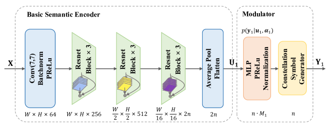
Figure 3: The NN framework of the JCM block. The output dimension of each layer is noted at the bottom.

In this paper, data transmission is carried out with $M$-QAM digital modulation by superposing $\mathbf{Y}_{1}$ and $\mathbf{Y}_{2}$. Each element in $\mathbf{Y}_{1}$ takes values from an $M_{1}$-QAM constellation $\mathcal{C}_{1}=\{c_{1}^{I}+j\cdot c_{1}^{Q}\}$, and each element in $\mathbf{Y}_{2}$ takes values from an $M_{2}$-QAM constellation $\mathcal{C}_{2}=\{c_{2}^{I}+j\cdot c_{2}^{Q}\}$, where $M_{1}$ and $M_{2}$ satisfy $M_{1}\times M_{2}=M$. The output of the transmitter, which we denote as $\mathbf{Y}\in\mathbb{C}^{n}$, is formed by

$$\mathbf{Y}=\sqrt{a}\mathbf{Y}_{1}+\sqrt{1-a}\mathbf{Y}_{2},$$ (3)

where $a$ denotes the power allocation factor (PAF), and we set $a\in(0.5,1)$ so that the inner constellation is truly “inner”. Note that before superposition, we respectively scale $\mathbf{Y}_{1}$ and $\mathbf{Y}_{2}$ so that they meet an average transmit power constraint $P$, i.e., $\frac{\|\mathbf{Y}_{1}\|^{2}}{n}=\frac{\|\mathbf{Y}_{2}\|^{2}}{n}=P$. Receiver 1 receives a sequence $\mathbf{Z}_{1}=\mathbf{Y}+\bm{\epsilon}_{1}$, where $\bm{\epsilon}_{1}\sim\mathcal{CN}(0,\sigma^{2}_{1})$. Similarly, Receiver 2 receives a sequence $\mathbf{Z}_{2}=\mathbf{Y}+\bm{\epsilon}_{2}$ with $\bm{\epsilon}_{2}\sim\mathcal{CN}(0,\sigma^{2}_{2})$ and $\sigma_{1}>\sigma_{2}$. The channel condition of Receiver $i$ ($i=1,2$) is characterized by the channel SNR, which is defined as $\frac{P}{\sigma_{i}^{2}}$. Fig. 2 displays examples of superposed inner and outer constellations (which we henceforward call super-constellations). Fig. 2(a), (b), and (c) depict the super-constellation resulting from the superposition of two 4QAM constellations, denoted as the 4QAM$\times$4QAM super-constellations. Fig. 2(d), (e), and (f) illustrate the super-constellation obtained by superposing a 4QAM inner constellation and a 16QAM outer constellation, denoted as the 4QAM$\times$16QAM super-constellation. As a side note, the $M$-QAM digital modulation can be easily extended to other modulation schemes, such as $M$-PSK.

At each receiver, two decoders are deployed. The decoders at Receiver 1 are denoted as

$$\mathbf{\hat{S}}_{1} =g_{\bm{\psi}_{1}}(\mathbf{Z}_{1}),$$ (4)

$$\mathbf{\hat{X}}_{1} =g_{\bm{\eta}_{1}}(\mathbf{Z}_{1}),$$ (5)

where $\bm{\psi}_{1}$ parameterizes the decoder for classification and $\bm{\eta}_{1}$ parameterizes the decoder for image recovery. Similarly, the decoders at Receiver 2 are denoted as

$$\mathbf{\hat{S}}_{2} =g_{\bm{\psi}_{2}}(\mathbf{Z}_{2}),$$ (6)

$$\mathbf{\hat{X}}_{2} =g_{\bm{\eta}_{2}}(\mathbf{Z}_{2}),$$ (7)

with $\bm{\psi}_{2}$ and $\bm{\eta}_{2}$ respectively parameterizing the decoder for classification and image recovery.

III Transmitter Design

The core of our DeepSCM scheme lies in transmitter design, which aims at extracting uncorrelated semantic features and generating the inner and outer constellation sequences in the superposition structure. Therefore, this section is dedicated to describing the components of the transmitter as well as the training algorithm. We first discuss the basic building block of the transmitter, namely the JCM block. Then, in III-B, we explain the technical detail of the aforementioned LMMSE decorrelator. Finally, in III-C, we present the training algorithm of the whole system.

III-A Joint Coding-Modulation

Extending our previous work[23, 24] to a broadcast setting, we use two JCM blocks to enable the digital modulation of two encoded feature vectors. The NN framework of the first JCM block is shown in Fig. 3. The basic semantic encoder includes multiple Resnet blocks[18] to map an image $\mathbf{X}$ of dimension $W\times H\times C$ into the basic encoded feature vector $\mathbf{U}_{1}$ of dimension $2n$, where $W$, $H$ and $C$ respectively denote the width, height and channel of the image, and we have $k=W\times H\times C$.

We then modulate $\mathbf{U}_{1}$ to obtain $\mathbf{Y}_{1}$. The modulation process is learned as a probabilistic model to avoid the inherent nondifferentiability problem. A multi-layer perceptron (MLP) with a $\text{PReLu}(\cdot)$ activation function and a normalization layer outputs the transition probability, $p(\mathbf{y}_{1}|\mathbf{u}_{1},\bm{\alpha}_{1})$. Since $\mathbf{Y}_{1}$ is discretely distributed with $M_{1}^{n}$ possible values, the transition probability is a discrete probability distribution with $M_{1}^{n}$ categories. To simplify the learning, we model each element of $\mathbf{Y}_{1}$ to be conditionally independent. Therefore, the total number of probability categories to be learned for $\mathbf{Y}_{1}$ decreases to $n\cdot M_{1}$. That is, for each element of $\mathbf{Y}_{1}$, the MLP respectively outputs $M_{1}$ un-normalized probabilities, which is then normalized to be a probability distribution. Based on this probability distribution, the constellation symbol generator, using a differentiable sampling technique called the Gumbel-Softmax[38], samples a constellation symbol for this element.

The enhancement semantic encoder and the modulator in the second JCM block follow the same framework. However, different from the first JCM block, before modulating $\mathbf{U}_{2}$, we first decorrelate it with $\mathbf{U}_{1}$.

TABLE II: The NN architecture of the proposed scheme, where $n$ is the number of channel uses.

	Layer	Output Dimension
Basic Semantic Encoder$\ \setminus$ Enhancement Semantic Encoder	Conv + BatchNorm + PReLU	32$\times$32$\times$64
	Resnet Block $\times$ 3	32$\times$32$\times$256
	Resnet Block $\times$ 3	16$\times$16$\times$512
	Resnet Block $\times$ 3	2$\times$2$\times$2n
	Average Pool + Flatten	2n
Modulator 1	MLP + PReLU	$n\cdot 2\sqrt{M_{1}}$
LMMSE Decorrelator	MLP	$2n$
Modulator 2	MLP + PReLU	$n\cdot 2\sqrt{M_{2}}$
Semantic Decoder for Classification at Receiver 1	Spinalnet Block $\times$ 4 + MLP	20
Semantic Decoder for Classification at Receiver 2	Spinalnet Block $\times$ 4 + MLP	100
Semantic Decoder for Image Recovery at Receiver 1 $\setminus$ Receiver 2	Conv + BatchNorm + ReLU	4$\times$4$\times$512
	Resnet Block $\times$ 2	4$\times$4 $\times$512
	Reshape + Conv + BatchNorm + ReLU	16$\times$16$\times$256
	Resnet Block $\times$ 2	16$\times$16$\times$256
	Reshape + Conv + BatchNorm + Sigmoid	32$\times$32$\times$3

III-B LMMSE Decorrelator

Due to the hierarchical relationship of the semantics, the enhanced encoded feature vector $\mathbf{U}_{2}$ is highly correlated with the basic encoded feature vector $\mathbf{U}_{1}$. Directly superposing them will cause redundancy in transmission and decrease the transmission efficiency.

To achieve maximum transmission efficiency, it is important that the encoded feature vectors being superposed should be independent. However, since independence between two variables is difficult to achieve, our goal is to remove from $\mathbf{U}_{2}$ the information that is highly correlated with $\mathbf{U}_{1}$ so that we can obtain a low-rate encoded feature vector that carries supplementary information from $\mathbf{U}_{1}$. We call this low-rate encoded feature vector the successive refinement vector $\mathbf{R}$ of $\mathbf{U}_{1}$. In other words, we want to find both a function $F(\cdot)$ and a vector $\mathbf{R}$, so that $\mathbf{U}_{2}$ can be written as

$$\mathbf{U}_{2}=F(\mathbf{U}_{1})+\mathbf{R},$$ (8)

where $\mathbf{R}$ should be low-rate since it carries less information. For simplicity, in this paper we choose a linear model for $F(\cdot)$. Hence, $\mathbf{U}_{2}$ can be written as

$$\mathbf{U}_{2} =F(\mathbf{U}_{1})+\mathbf{R}$$

$$=\mathbf{WU}_{1}+\mathbf{b}+\mathbf{R},$$ (9)

where matrix $\mathbf{W}\in\mathbb{R}^{2n\times 2n}$ and vector $\mathbf{b}\in\mathbb{R}^{2n}$ are parameters to be determined so that a low-rate $\mathbf{R}$ can be obtained. However, it is hard to directly optimize the entropy of $\mathbf{R}$, given the challenge of estimating the entropy rate of a random variable. The following proposition presents an alternative approach to finding a low-rate $\mathbf{R}$.

Proposition 1 (Upperbound of the entropy)

The entropy of $\mathbf{R}$ is upperbounded by

$$h(\mathbf{R})\leq n\log\frac{\pi e}{n}\mathbf{E}[||\mathbf{R}||_{2}^{2}].$$ (10)

The proof can be found in Appendix A. As can be seen, the upperbound of the entropy of $\mathbf{R}$ is decided by the term $\mathbf{E}[||\mathbf{R}||_{2}^{2}]$. Therefore, minimizing the entropy of $\mathbf{R}$ can be translated into minimizing its expected $l_{2}$ norm. Expanding the term $\mathbf{E}[||\mathbf{R}||_{2}^{2}]$, we can get

$$\mathbf{E}[||\mathbf{R}||_{2}^{2}]=\mathbf{E}[(\mathbf{U}_{2}-\mathbf{WU}_{1}-\mathbf{b})^{T}(\mathbf{U}_{2}-\mathbf{WU}_{1}-\mathbf{b})].$$ (11)

In our DeepSCM scheme, we utilize a one-layer MLP for $F(\cdot)$ with input $\mathbf{U}_{1}$ and output ${\mathbf{W}}\mathbf{U}_{1}+\mathbf{b}$, where $\mathbf{W}$ and $\mathbf{b}$ respectively represent the weights and bias of the one-layer MLP. The optimization problem is thus established as

$$\underset{\mathbf{W},\mathbf{b}}{\mathrm{min}}\ \ \mathbf{E}[(\mathbf{U}_{2}-\mathbf{W}\mathbf{U}_{1}-\mathbf{b})^{T}(\mathbf{U}_{2}-\mathbf{W}\mathbf{U}_{1}-\mathbf{b})].$$ (12)

Notice that, the global optimal solution of this minimization problem is the LMMSE estimation of $\mathbf{U}_{2}$ given $\mathbf{U}_{1}$, where

$$\mathbf{W}^{\ast} =\textit{Cov}[\mathbf{U}_{2},\mathbf{U}_{1}]\textit{Var}[\mathbf{U}_{1}]^{-1},$$ (13)

$$\mathbf{b}^{\ast} =\mathbf{E}[\mathbf{U}_{2}]-\mathbf{W}^{\ast}\mathbf{E}[\mathbf{U}_{1}].$$ (14)

Moreover, following the orthogonality principle of linear estimators [39, p.386], the global optimal $\mathbf{R}^{\ast}$ which serves as the estimation error, is uncorrelated with $\mathbf{U}_{1}$, i.e.,

$$\mathbf{E}[\mathbf{U}_{1}\mathbf{R}^{\ast T}]=\mathbf{0}.$$ (15)

In other words, the correlation between the $\mathbf{U}_{1}$ and $\mathbf{R}$ can indeed vanish with a sufficient number of training samples.

III-C Training Strategy

As can be seen, there are a total of nine NN modules used in the proposed scheme for different purposes. The intricate design of this framework makes it difficult to ensure the convergence of the network training. Therefore, we adopt a three-stage training strategy for our DeepSCM scheme. In the first stage, the encoding and decoding NNs for the generation of the inner constellation sequence are trained, namely the first JCM block and the decoders at Receiver 1. Then in the second stage, we further train the encoding and decoding NNs for the generation of the outer constellation sequence, including the second JCM block and the decoders at Receiver 2 while freezing other parameters. In the last training stage, the whole system is fine-tuned jointly to further improve its overall performance.

As a commonly used method[23, 13], we employ the cross entropy (CE) as the distortion measure function to evaluate the quality of classification, and the MSE to measure the distortion between the raw image and its recovery. Therefore, the loss function for the first training stage can be formulated as

$$\mathcal{L}_{1}(\bm{\theta}_{1},\bm{\alpha}_{1},\bm{\psi}_{1},\bm{\eta}_{1})=CE(\mathbf{S}_{1},\mathbf{\hat{S}}_{1})+\lambda_{1}\cdot MSE(\mathbf{X},\mathbf{\hat{X}}_{1}),$$ (16)

where $\lambda_{1}$ represents the hyperparameter to balance the two tasks, as used in many previous works[37, 12].

Similarly, the loss function of the second stage includes CE for fine classification, MSE for image recovery, and the objective in (12) as an additional regularizer, which can be written as

$$\ \ \ \ \ \ \ \ \ \ \ \ \ \mathcal{L}_{2}(\bm{\theta}_{2},\bm{\alpha}_{2},\mathbf{W},\mathbf{b},\bm{\psi}_{2},\bm{\eta}_{2})=$$

$$CE(\mathbf{S}_{2},\mathbf{\hat{S}}_{2})+\lambda_{2}\cdot MSE(\mathbf{X},\mathbf{\hat{X}}_{2})+\lambda_{3}\cdot\|\mathbf{R}\|^{2}_{2},$$ (17)

with $\lambda_{2}$ and $\lambda_{3}$ being two hyperparameters. Finally, the loss function in the fine-tuning stage is the combination of $\mathcal{L}_{1}$ and $\mathcal{L}_{2}$, which is expressed as

$$\mathcal{L}_{3}(\bm{\theta}_{1},\bm{\alpha}_{1},\bm{\psi}_{1},\bm{\eta}_{1},\bm{\theta}_{2},\bm{\alpha}_{2},\mathbf{W},\mathbf{b},\bm{\psi}_{2},\bm{\eta}_{2})=\mathcal{L}_{1}+\beta\cdot\mathcal{L}_{2},$$ (18)

where $\beta$ is used to balance the importance of the two receivers.

IV Experiment Results

In this section, we use simulations to validate the advantages of our proposed DeepSCM scheme. We first present the experiment settings in Section IV-A. Then, we compare the performance of the DeepSCM scheme with benchmarks across various transmission rates and levels of channel disparity respectively in Section IV-B and IV-C. Furthermore, to establish guidelines for determining the PAF, we conduct experiments in Section IV-D examining its impacts on the training process and the overall system performance.

TABLE III: Detailed learning rate and number of training epochs for each stage.

Stage	Number of Training Epochs	Initial LR	Scheduler
1	100	2e-4	Cosine Annealing Warm Restarts with Final LR=1e-5
2	150	2e-4
3	50	5e-5

IV-A Experiment Settings

IV-A1 Dataset

Our experiments are conducted on the CIFAR100 dataset[40], which includes 50000 training images and 10000 test images. The resolution of each image is $32\times 32$. All images are classified into 20 super-categories, and images in each super-category are further classified to 5 sub-categories[40]. The 20-category classification label of each image stands for its coarse-grained semantic source $\mathbf{S}_{1}$ while the 100-category classification label of each image stands for its fine-grained semantic source $\mathbf{S}_{2}$.

IV-A2 NN Architecture and Hyperparameters

The transmitter design has been presented in Section III. For decoders, we adopt Spinal-net[41] for coarse classification as well as fine classification. The semantic decoders for image recovery at both receivers have the same NN architecture, which consists of Resnet blocks combined with the depth-to-space operation to perform the upsampling. Table II presents the details of the NN architecture we use in this paper. We employ the Adam optimizer for the training. The detailed learning rate (LR) schedule is shown in Table III. The experiments are conducted using two super-constellations: 4QAM$\times$4QAM and 4QAM$\times$16QAM. We set the value of the power allocation factor $a$ such that the super-constellations form rectangular QAM constellation. Specifically, for 4QAM$\times$4QAM, we set $a=0.80$, and for 4QAM$\times$16QAM, we set $a=0.76$. All the experiments are performed on Intel Xeon Silver 4214R CPU, and 24 GB Nvidia GeForce RTX 3090 Ti graphics card with Pytorch powered with CUDA 11.4.

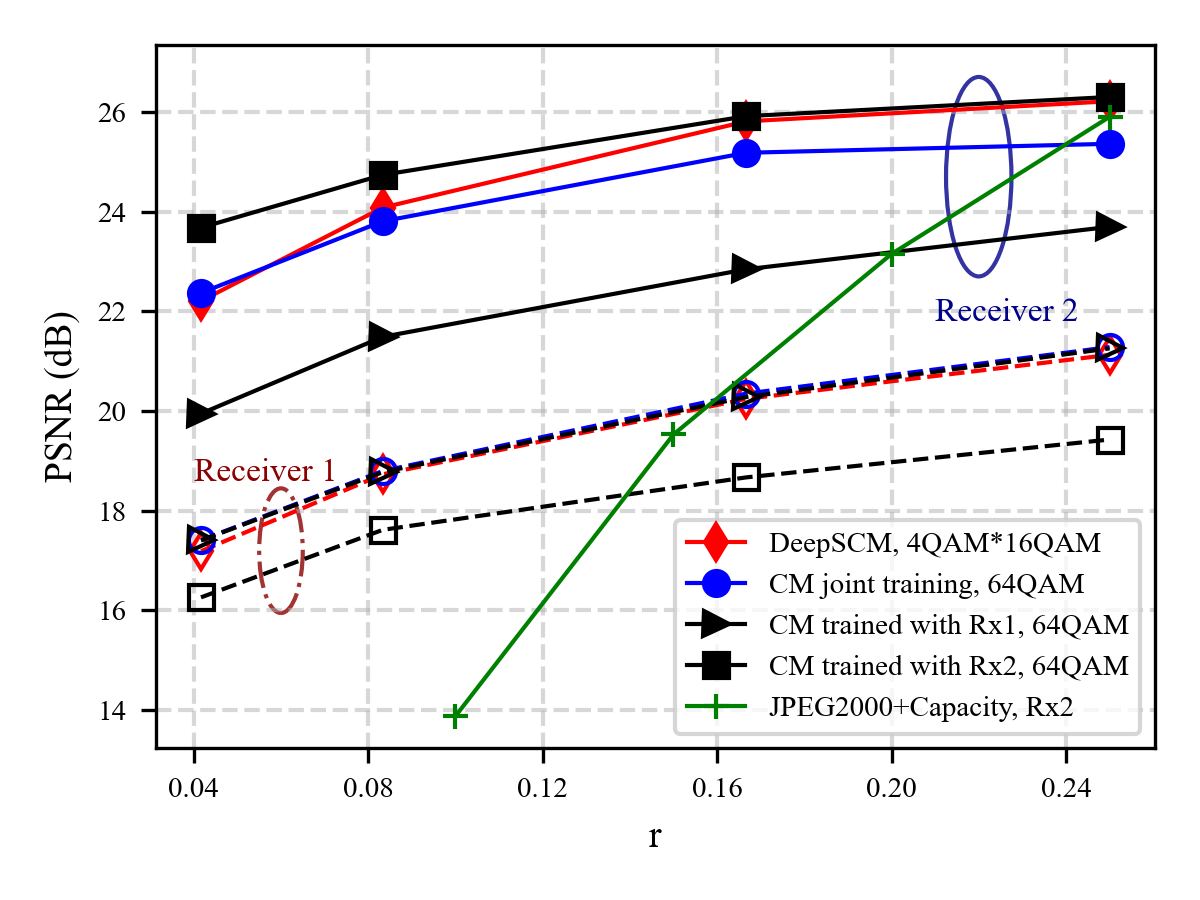
(a) Image recovery vs. $r$.

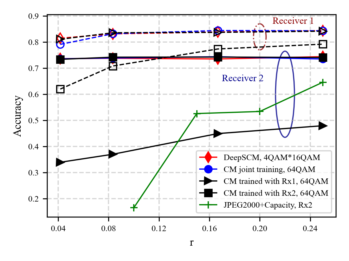
(b) Classification accuracy vs. $r$.

Figure 4: Performances of the DeepSCM scheme and the benchmarks at varying transmission rates, with the super-constellation set as 4QAM$\times$16QAM.

IV-A3 Benchmarks

We compare the proposed DeepSCM scheme with the conventional unstructured coded modulation (CM) scheme using rectangular $M$-QAM modulation, where only one semantic encoder is utilized at the transmitter. Additionally, we compare our DeepSCM scheme with classical separation-based source and channel coding scheme for a single receiver, where JPEG2000 and ideal capacity-achieving channel code are employed (abbreviated as “JPEG2000+Capacity”). In the CM scheme, the NN architecture of the semantic encoder, modulator and the two receivers are the same as their counterparts in our proposed DeepSCM scheme. We employ three different training methods for the CM scheme as three benchmarks.

• CM Joint Training: In this scheme, the transmitter and the two receivers are jointly trained. Specifically, the loss function is set to be a weighted sum of the distortion measures of both receivers, which means that the transmitter balances the feedback from both receivers.

• CM Trained with Rx1: Following the training method in [34], in this scheme, the transmitter is jointly trained with Receiver 1 in the absence of Receiver 2. After the transmitter is trained and fixed, the decoders at Receiver 2 is then trained to achieve its best possible performance. Note that this scheme serves as the performance upperbound for Receiver 1 under the CM scheme.

• CM Trained with Rx2: This training scheme follows the same idea of “CM Trained with Rx1” but exchanges the role of Receiver 1 and Receiver 2. Similarly, it serves as the performance upperbound for Receiver 2 under the CM scheme.

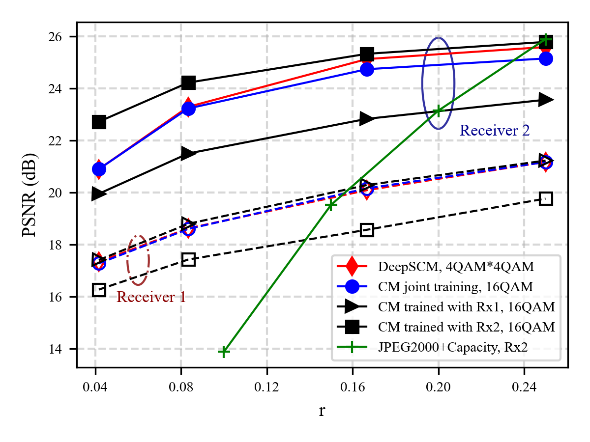
(a) Image recovery vs. $r$.

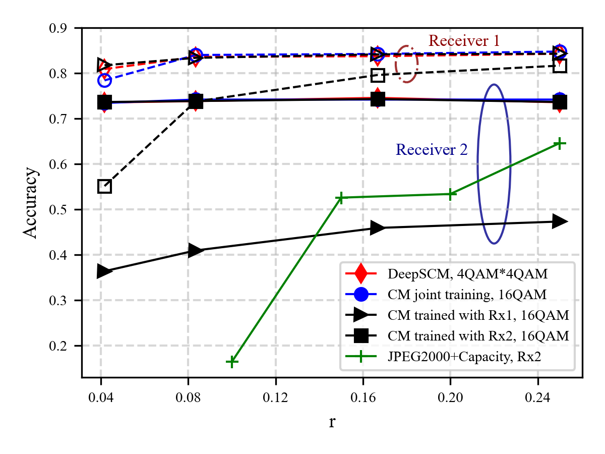
(b) Classification accuracy vs. $r$.

Figure 5: Performances of the DeepSCM scheme and the benchmarks at varying transmission rates, with the super-constellation set as 4QAM$\times$4QAM.

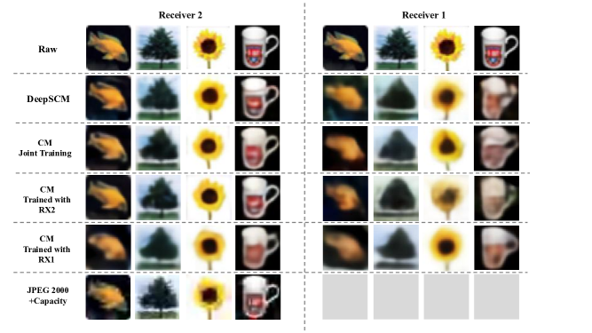
Figure 6: Visual examples of the image recovered by different schemes for Receiver 1 and Receiver 2 with $M=64$ and $r=\frac{1}{6}$.

IV-A4 Performance Metrics

For the coarse and fine classification tasks, we use classification accuracy to evaluate the performance. For the image recovery task, we use peak-signal-to-noise ratio (PSNR) to denote the performance, which is defined as

$$\text{PSNR}=10\log\frac{\text{MAX}^{2}}{\text{MSE}},$$ (19)

where MAX is the maximum possible pixel value of the image. We define the transmission rate $r$ as the ratio between the number of channel uses and the dimension of the images, i.e.,

$$r=\frac{n}{k},$$ (20)

where for CIFAR100, $k=32\times 32\times 3$.

IV-B Performances at Varying Transmission Rates

In this subsection, we compare the performances of the DeepSCM scheme and the benchmarks when the transmission rate varies from $\frac{1}{24}$ (128 channel uses) to $\frac{1}{4}$ (768 channel uses). If not specified otherwise, we set the channel SNR of Receiver 1 as $-5$ dB and that of Receiver 2 as 20 dB.

Fig. 4 focuses on the case when a 4QAM$\times$16QAM super-constellation is used for our proposed DeepSCM scheme. Fig. 4(a) illustrates the PSNR performance of image recovery of Receiver 1 and Receiver 2 versus different transmission rates. Overall we can observe that the PSNRs of the proposed DeepSCM scheme for both receivers are very close to their respective upperbound. Specifically, for Receiver 1, the performance of the proposed scheme nearly coincides with the performance upperbound, the CM trained with Rx1 scheme, outperforming the CM trained with Rx2 scheme by more than 1 dB. Notice that we omit the performance of JPEG2000$+$Capacity for Receiver 1, since this scheme completely breaks down under the poor channel condition of Receiver 1. For Receiver 2, the performance of the proposed scheme approaches the performance upperbound, the CM trained with Rx2 scheme, and coincides with it when $r$ is high. The proposed scheme outperforms the CM joint training scheme by 0 dB to 1 dB, and outperforms the CM trained with Rx2 scheme by more than 2 dB. Moreover, the proposed scheme has a great advantage over the conventional separate coding scheme, particularly at lower transmission rates.

Fig. 4(b) illustrates the performances of Receiver 1 and Receiver 2 in terms of classification accuracy. Notably, the classification accuracies of the two receivers are not directly comparable as Receiver 1 only needs to classify 20 categories while Receiver 2 needs to do 100 categories. Similar to the performances of image recovery, the classification accuracy of our proposed DeepSCM scheme are also close to the upperbound performances of both Receiver 1 and 2 and outperforms other benchmarks. For example, when $r=\frac{1}{24}$, the proposed DeepSCM scheme has a coarse classification accuracy of 81.5$\%$, which is the same as that of the CM trained with Rx1 scheme, and surpasses the CM joint training scheme by 2.4$\%$, and the CM trained with Rx2 scheme by 19.5$\%$. Furthermore, the performance of the fine classification accuracy of the DeepSCM scheme coincides with its upperbound, and greatly exceeds the CM trained with Rx1 scheme and the conventional separate coding scheme.

Meanwhile, Fig. 5 focuses on the cases where a 4QAM$\times$4QAM super-constellation is used. Similar to the case with a 4QAM$\times$16QAM super-constellation, our proposed scheme can achieve the upperbound performance of both Receiver 1 and 2 simultaneously for classification and image recovery. For Receiver 2, our scheme approaches the upperbound with increasing $r$, constantly outperforms the CM joint training scheme and the CM trained with Rx1 scheme, and significantly outperforms the JPEG 2000$+$Capacity scheme when $r$ is low. For example, in image recovery, when $r=\frac{1}{6}$, the performance of the proposed DeepSCM scheme exceeds that of the CM trained with Rx1 scheme by 2.3 dB, exceeds that of the CM joint training scheme by 0.4 dB, and exceeds that of the JPEG 2000$+$Capacity scheme by more than 4 dB. Furthermore, for Receiver 1, our scheme has close performance to the upperbound, the CM trained with Rx1 scheme, and outperforms other benchmarks. When $r=\frac{1}{24}$, the coarse classification accuracy of the DeepSCM scheme reaches 80.9$\%$, only 0.8$\%$ lower than the upperbound, and exceeds that of the CM joint training scheme by 2.5$\%$, and that of the CM trained with Rx2 scheme by more than 30$\%$.

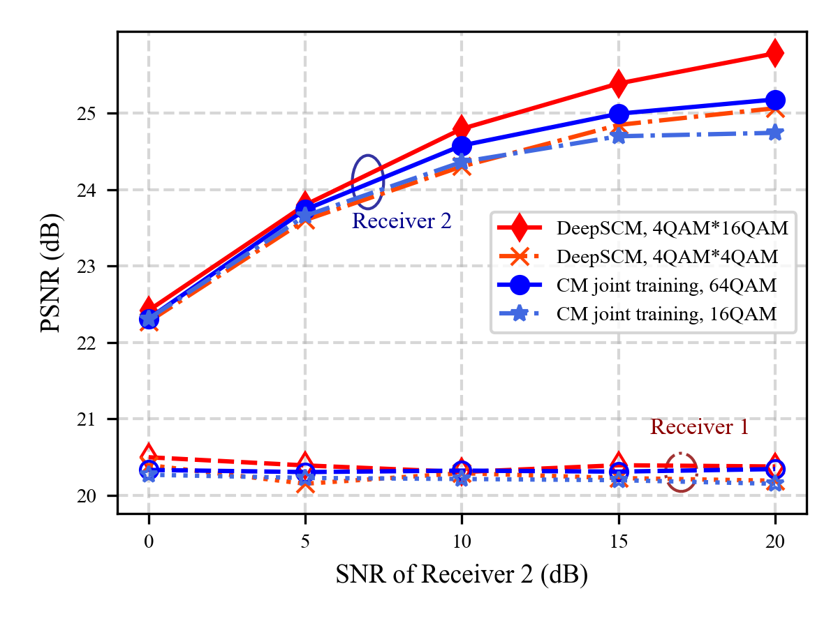
(a) The image recovery vs. SNR.

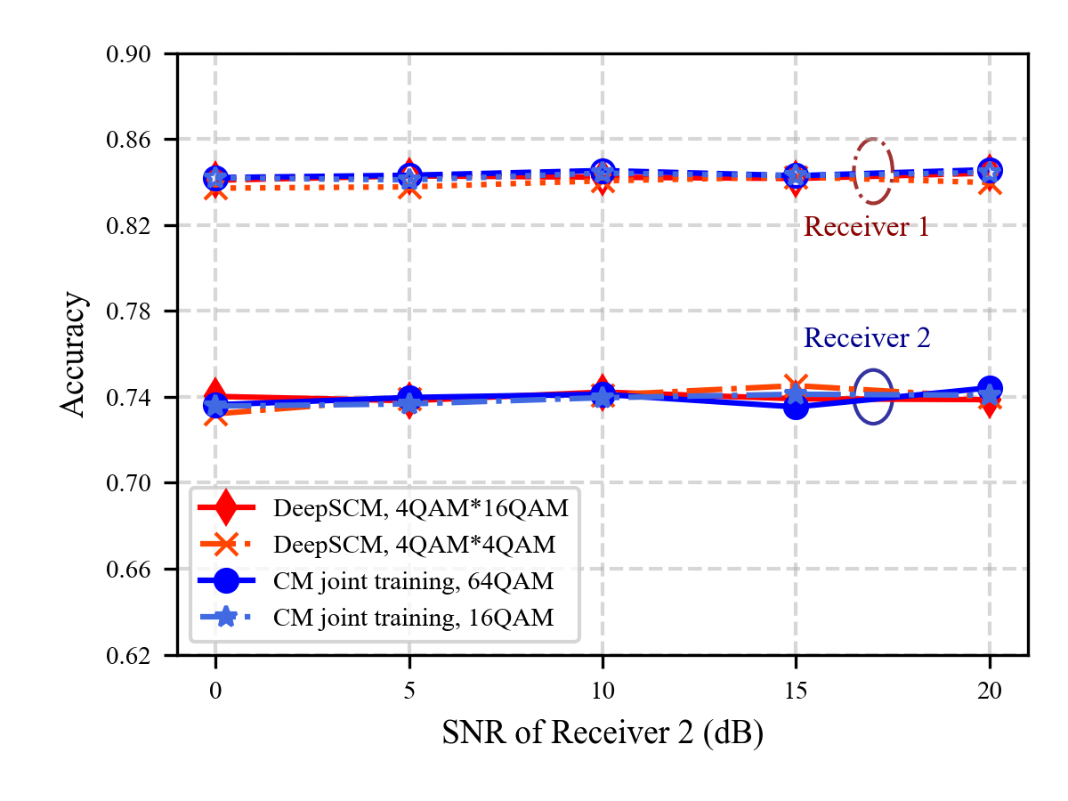
(b) Classification accuracy vs. SNR.

Figure 7: The performance comparison of the DeepSCM scheme and the CM joint training scheme at different channel SNR values of Receiver 2.

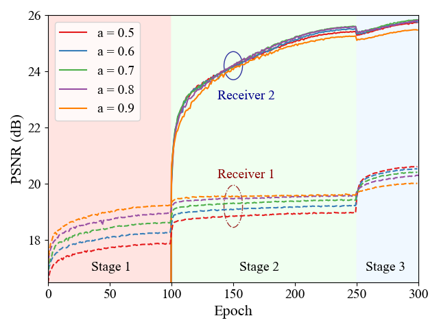
(a) The convergence curve of image recovery.

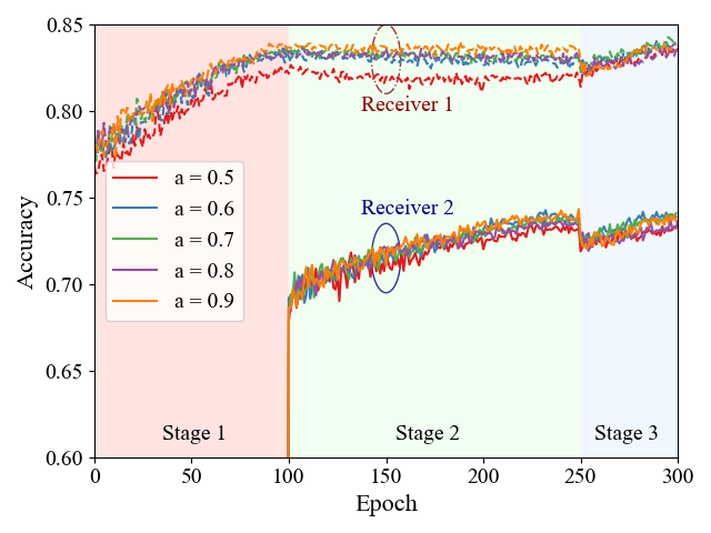
(b) The convergence curve of classification accuracy.

Figure 8: The convergence curve of the DeepSCM scheme with different $a$.

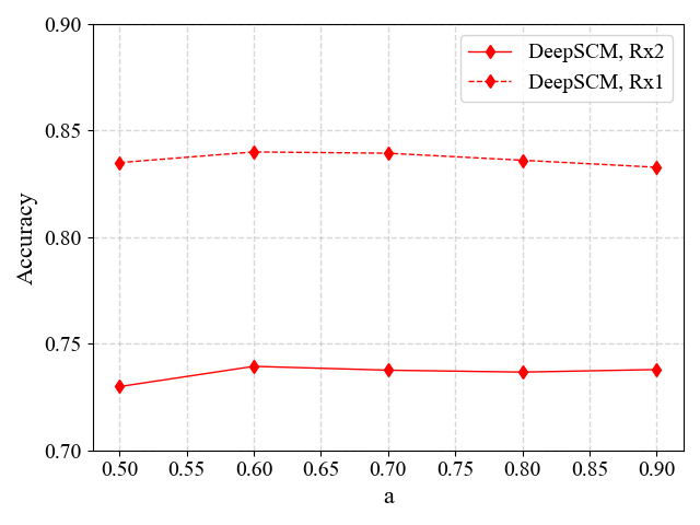
(a) Image recovery vs. $a$.

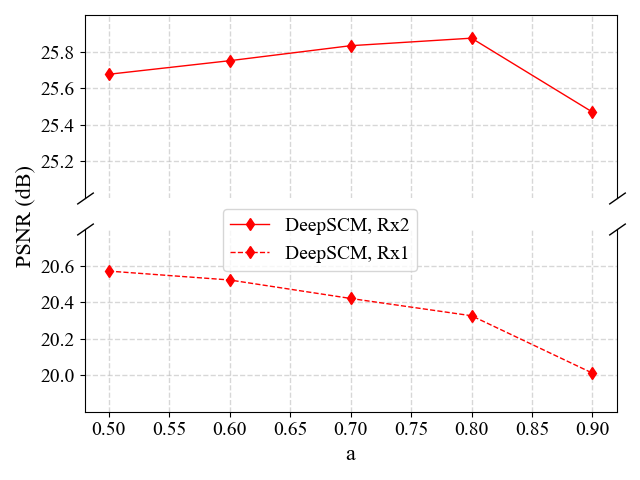
(b) Classification accuracy vs. $a$.

Figure 9: Performance of the DeepSCM scheme with varying $a$.

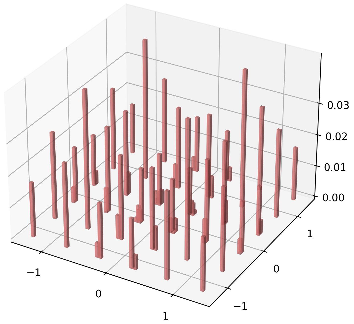
(a) $a=0.5$.

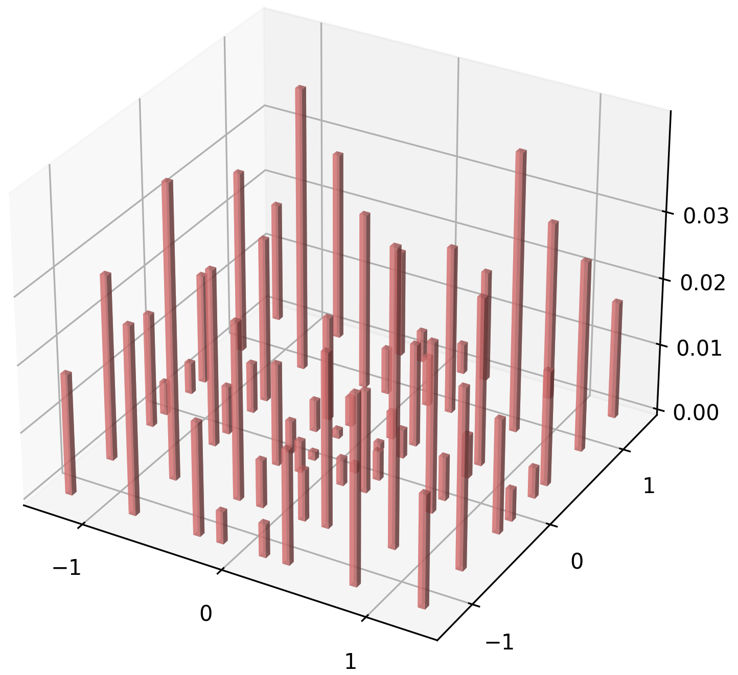
(b) $a=0.6$.

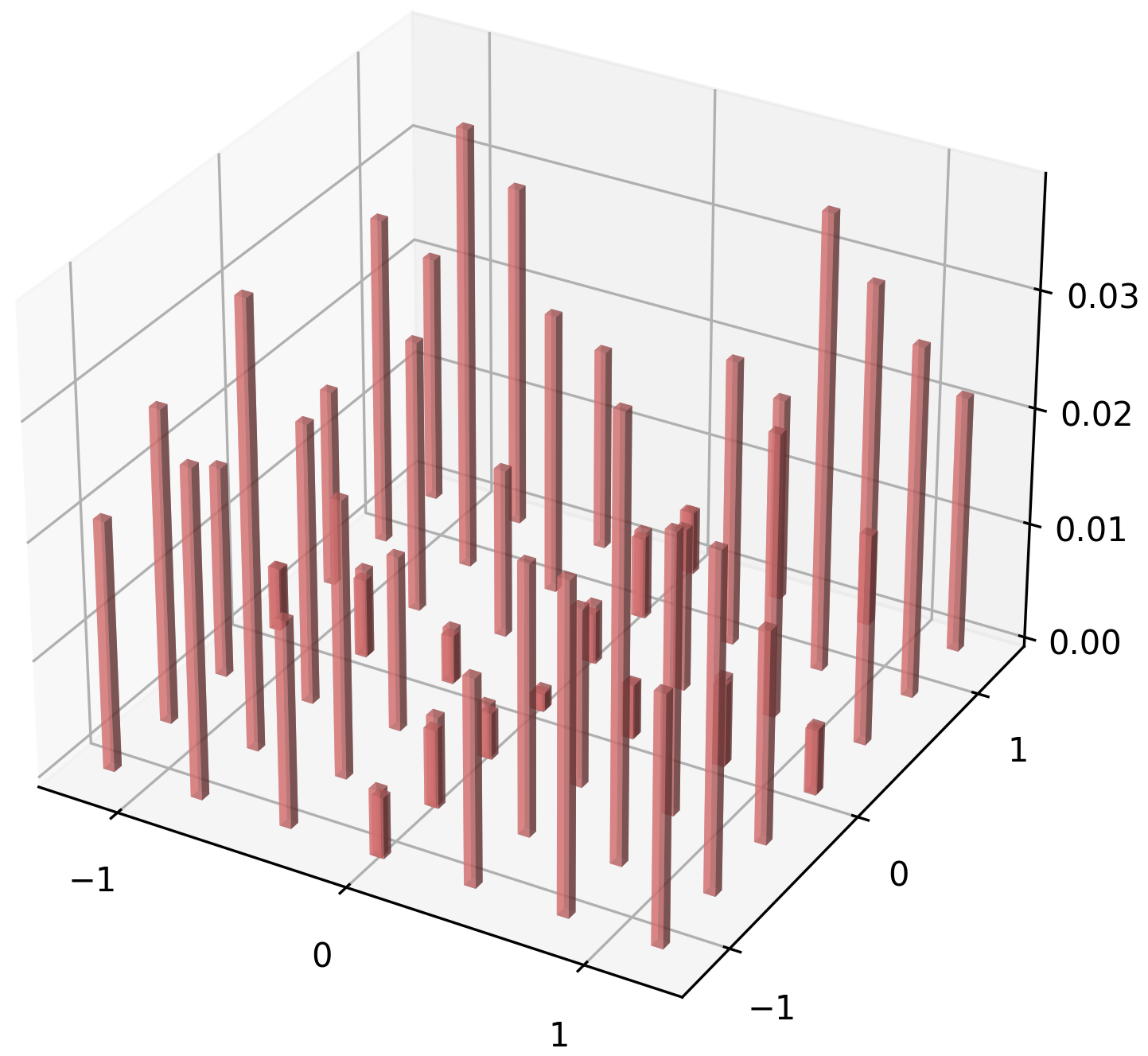
(c) $a=0.7$.

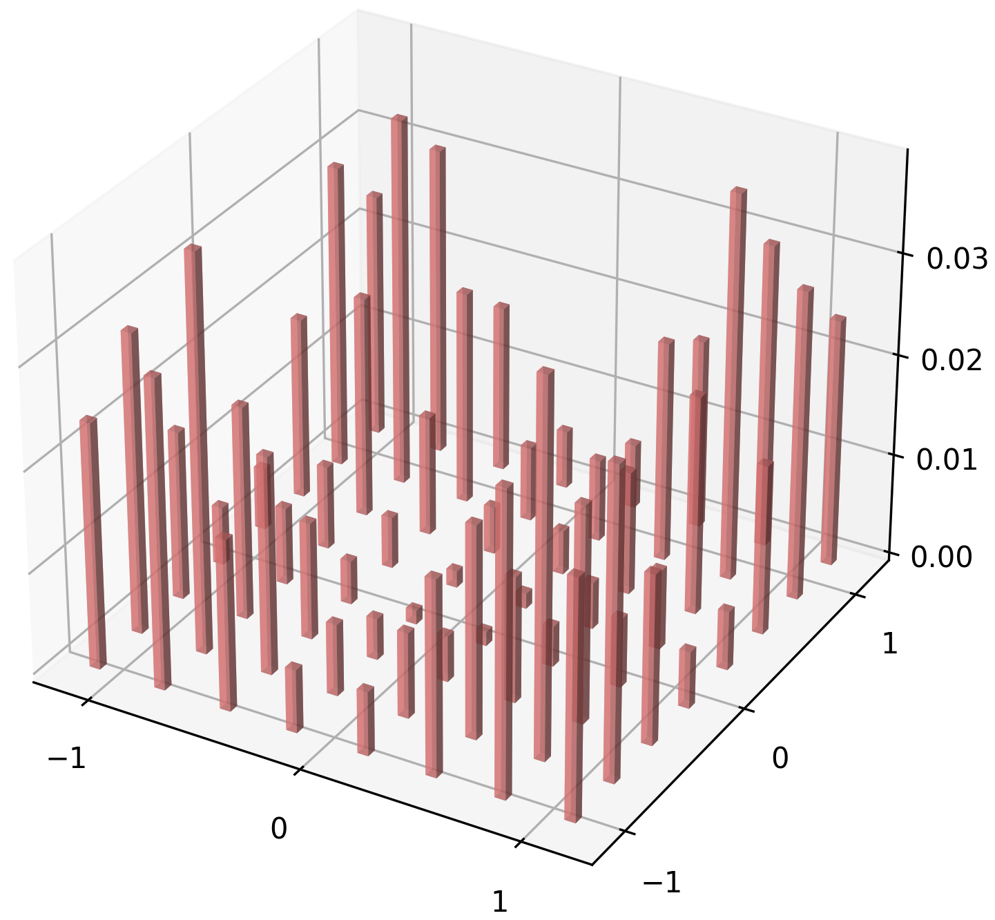
(d) $a=0.8$.

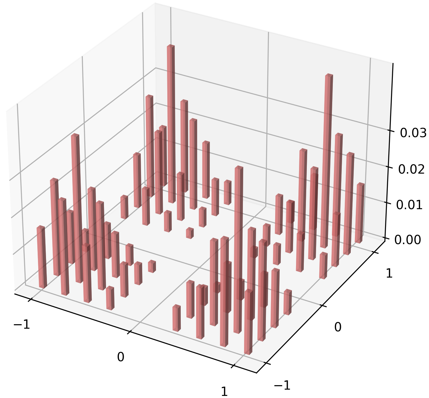
(e) $a=0.9$.

Figure 10: The empirical distributions of the 4QAM$\times$16QAM super-constellation points with different PAF values.

Fig. 6 displays visual examples of the image recovered by different schemes for Receiver 1 and Receiver 2. We can observe that for Receiver 2, the proposed DeepSCM scheme, along with the CM trained with Rx2 scheme, attains the highest quality in recovered images. The images recovered by the CM joint training scheme and the CM trained with Rx1 scheme appear more blurred, indicating their inferior performances. Moreover, compared with the images recovered by the DeepSCM scheme, those recovered from JPEG 2000 compression display a loss of sharpness around high-contrast edges and exhibit a blocky structure. These JPEG artifacts negatively affect the visual quality of the images. In contrast to the images of Receiver 2, those of Receiver 1 exhibit lower quality due to its poor channel condition. Furthermore, since Receiver 1 has a smaller channel capacity, it cannot decode the images encoded by the JPEG 2000 compression algorithm and the capacity-achieving channel coding of Receiver 2, which shows the limitations of the conventional separate coding scheme in a broadcast channel.

All in all, simulation results show that the proposed superposition code structure is indeed efficient in degraded broadcast channels. It alleviates the conflict between diverse semantic information granularity requirements of the two receivers with different channel conditions, improving the performance of both receivers instead of sacrificing the performance of one receiver to improve that of the other.

IV-C Performances versus Channel Disparity

In this subsection, we compare the performance of our proposed DeepSCM scheme and that of the CM joint training scheme at varying levels of channel disparity, namely different SNR gaps between Receiver 1 and Receiver 2. Specifically, we fix the channel SNR of Receiver 1 as $-5$ dB, and vary the channel SNR of Receiver 2 from 0 dB to 20 dB. The transmission rate is set as $\frac{1}{6}$ (512 channel uses).

Fig. 7 shows the performances of the DeepSCM scheme and the benchmarks at different levels of channel disparity. We tune the hyperparameters $\lambda_{1}$ and $\lambda_{2}$ so that the two schemes have the same performance in the classification task, as shown in Fig. 7(b), and we compare their performances in the image recovery task, illustrated in Fig. 7(a). Two important observations can be made. First, our scheme has an increasing performance advantage over the joint training scheme as the channel disparity increases. For example, when using a 4QAM$\times$4QAM super-constellation, the performance of our scheme at Receiver 2 and that of the joint training scheme almost coincide when the channel disparity is lower than 15 dB. When the channel disparity rises up to 25 dB, our scheme outperforms the joint training scheme by 0.3 dB. Additionally, we can see that higher modulation order will further enlarge the performance gap between our scheme and the joint training scheme. For example, when the channel disparity is 25 dB, or equivalently, the SNR of Receiver 2 is 20 dB, the performance advantage of our scheme can reach 0.6 dB when a 4QAM$\times$16QAM super-constellation is used, 0.3 dB higher than the performance advantage when a 4QAM$\times$4QAM super-constellation is used.

In conclusion, the stimulation results show that our scheme exhibits a performance advantage over the CM joint training scheme that correlates positively with the communication capability gap between the two receivers. Specifically, when there is a larger disparity in channel SNR between the receivers or when the system supports a higher modulation order, our scheme yields greater benefits compared to the joint training scheme due to its superposition coding structure.

IV-D Impact of PAF

Since power allocation between different receivers is an important issue in classical superposition code, in this subsection, we investigate the impact of the hyperparameter PAF by varying $a$ from 0.5 to 0.9. The experiment is conducted using the 4QAM$\times$16QAM super-constellation. The channel SNR for Receiver 1 is set to -5 dB, while Receiver 2 has an SNR of 20 dB. We fix the parameter $r$ at $\frac{1}{6}$, equivalent to 512 channel uses. Intuitively, there should be a performance trade-off between the two receivers. Allocating more power to the inner constellation points will improve the performance of Receiver 1, and vice versa.

Fig. 8 shows the convergence curve of the DeepSCM scheme with different values of $a$, illustrating their impact on each training stage of the DeepSCM scheme. Fig. 8(a) shows the convergence curve of image recovery. We can indeed observe a performance trade-off between the two receivers during the first two stages. In Stage 1 when Receiver 1 is trained, larger values of $a$ result in better performance of Receiver 1, which is attributed to the fact that the superposed outer constellation points serve as additional noise. In Stage 2 when Receiver 2 is trained, larger values of $a$ (e.g., $a=0.9$) lead to worse performance for Receiver 2. However, this intuitive performance trade-off disappears during the fine-tuning stage, where larger values of $a$ also lead to decreased performance for Receiver 1. This indicates that Receiver 1 can still decode the outer constellation to some extent due to the powerful adaptability of NNs to channel noise. The influence of $a$ on the performance of classification in Fig. 8(b) is less obvious, yet similar observations can be made.

Fig. 9 further shows the performance of the DeepSCM scheme with varying values of $a$. Fig. 9(a) shows the performance of image recovery of the two receivers. The performance of Receiver 1 decreases with increasing $a$. For Receiver 2, not only too large an $a$ causes its performance degradation, but too small an $a$ also leads to worse performance. This is because with smaller $a$, the outer constellation points will overlay, making it harder for Receiver 2 to decode them. In Fig. 9(b) we can also observe that extreme PAF values cause a decline in performance. Given our hierarchical-source scenario, it is important to note that the results differ from the scenario of broadcasting independent messages to two receivers. In the latter case, increasing $a$ enhances the performance of one receiver while diminishing that of the other.

Overall, these observations offer principles for determining the PAF: $a$ should be chosen to prevent the overlay of outer constellation points, and the interval between outer constellation points should not be too small. Therefore, it is best to choose moderate PAF values to achieve the overall best performance. Demonstrating that moderate PAF values are most reasonable significantly simplifies the selection of PAF. We can simply set $a$ such that the super-constellation forms rectangular QAM constellation, as in Section IV-B and Section IV-C.

In Figure 10, we illustrate the empirical distributions of the 4QAM$\times$16QAM super-constellation points with varying PAF values. It can be noted that the outer constellation points overlap with smaller $a$. Moreover, it is evident that due to the poor channel condition of Receiver 1, constellation points with lower power are less likely to be generated.

V Conclusion

This paper proposes a new framework for digital semantic communications over degraded AWGN broadcast channels, namely the DeepSCM scheme. In this scheme, the semantic features intended for different receivers are encoded into a basic encoded feature vector and its successive refinement vector, which are then associated with different layers of a super-constellation. To minimize redundancy in broadcasting, an LMMSE decorrelator is developed to ensure that these two vectors are nearly uncorrelated with each other. This superposition code structure can accommodate the communication requirements of different receivers with diverse channel conditions. The proposed scheme is especially effective in scenarios with large channel disparity and high modulation order. All in all, the proposed framework not only provides an efficient way to conduct semantic broadcasting, but also shows a promising future of combining theoretical coding schemes with NN-based coding method.

In the future, we plan to extend our superposition coding approach to other multi-user communication scenarios, such as the semantic communications for multi-terminal sources. Moreover, we will enhance the performance of our proposed scheme by introducing techniques such as superposition constellation shaping.

Appendix A Proof of Proposition 1

The proof of Proposition 1 follows a straightforward idea of upper-bounding the differential entropy of $\mathbf{R}$ step by step. The details are as follows.

$$h(\mathbf{R}) \overset{(a)}{\leq}\frac{1}{2}\log(2\pi e)^{2n}|\textit{Var}[\mathbf{R}]|$$

$$\overset{(b)}{\leq}\frac{1}{2}\log(2\pi e)^{2n}\textstyle\prod_{i=1}^{2n}\textit{Var}[R_{i}]$$

$$\overset{(c)}{\leq}\frac{1}{2}\log(2\pi e)^{2n}(\frac{\sum_{i=1}^{2n}\textit{Var}[R_{i}]}{2n})^{2n}$$

$$\overset{(d)}{\leq}n\log\frac{\pi e}{n}\sum_{i=1}^{2n}\mathbf{E}[R_{i}^{2}]$$

$$=n\log\frac{\pi e}{n}\mathbf{E}[||\mathbf{R}||^{2}_{2}],$$ (21)

where $R_{i}$ denotes the $i$th entry of $\mathbf{R}$, $|\textit{Var}[\mathbf{R}]|$ denotes the determinant of $\textit{Var}[\mathbf{R}]$, $(a)$ follows from the fact that Gaussian distribution maximizes entropy under a given covariance matrix, $(b)$ follows from Hadamard inequality since covariance matrices are always positive semidefinite, $(c)$ follows from the inequality of arithmetic and geometric means, and $(d)$ follows from the definition of variance that $\textit{Var}[R_{i}]=\mathbf{E}[R_{i}^{2}]-\mathbf{E}^{2}[R_{i}]$.

References

- [1] Y. Bo, S. Shao, and M. Tao, “A superposition code approach for digital semantic communications over broadcast channels,” in 2023 IEEE Globecom. IEEE, 2023, pp. 1–6.
- [2] D. Gündüz, Z. Qin, I. E. Aguerri, H. S. Dhillon, Z. Yang, A. Yener, K. K. Wong, and C.-B. Chae, “Beyond transmitting bits: Context, semantics, and task-oriented communications,” IEEE Journal on Selected Areas in Communications, vol. 41, no. 1, pp. 5–41, 2023.
- [3] Q. Lan, D. Wen, Z. Zhang, Q. Zeng, X. Chen, P. Popovski, and K. Huang, “What is semantic communication? a view on conveying meaning in the era of machine intelligence,” Journal of Communications and Information Networks, vol. 6, no. 4, pp. 336–371, 2021.
- [4] X. Luo, H.-H. Chen, and Q. Guo, “Semantic communications: Overview, open issues, and future research directions,” IEEE Wireless Communications, vol. 29, no. 1, pp. 210–219, 2022.
- [5] M. Sana and E. C. Strinati, “Learning semantics: An opportunity for effective 6g communications,” in 2022 IEEE 19th Annual Consumer Communications And Networking Conference (CCNC), 2022, pp. 631–636.
- [6] Z. Weng and Z. Qin, “Semantic communication systems for speech transmission,” IEEE Journal on Selected Areas in Communications, vol. 39, no. 8, pp. 2434–2444, 2021.
- [7] H. Xie, Z. Qin, G. Y. Li, and B.-H. Juang, “Deep learning enabled semantic communication systems,” IEEE Transactions on Signal Processing, vol. 69, pp. 2663–2675, 2021.
- [8] Q. Zhou, R. Li, Z. Zhao, C. Peng, and H. Zhang, “Semantic communication with adaptive universal transformer,” IEEE Wireless Communications Letters, vol. 11, no. 3, pp. 453–457, 2022.
- [9] H. Xie and Z. Qin, “A lite distributed semantic communication system for internet of things,” IEEE Journal on Selected Areas in Communications, vol. 39, no. 1, pp. 142–153, 2021.
- [10] J. Shao, Y. Mao, and J. Zhang, “Learning task-oriented communication for edge inference: An information bottleneck approach,” IEEE Journal on Selected Areas in Communications, vol. 40, no. 1, pp. 197–211, 2022.
- [11] K. Liu, D. Liu, L. Li, N. Yan, and H. Li, “Semantics-to-signal scalable image compression with learned revertible representations,” International Journal of Computer Vision, vol. 129, no. 9, pp. 2605–2621, 2021.
- [12] H. Zhang, S. Shao, M. Tao, X. Bi, and K. B. Letaief, “Deep learning-enabled semantic communication systems with task-unaware transmitter and dynamic data,” IEEE Journal on Selected Areas in Communications, vol. 41, no. 1, pp. 170–185, 2023.
- [13] E. Bourtsoulatze, D. Burth Kurka, and D. Gündüz, “Deep joint source-channel coding for wireless image transmission,” IEEE Transactions on Cognitive Communications and Networking, vol. 5, no. 3, pp. 567–579, 2019.
- [14] S. Wang, J. Dai, Z. Liang, K. Niu, Z. Si, C. Dong, X. Qin, and P. Zhang, “Wireless deep video semantic transmission,” IEEE Journal on Selected Areas in Communications, vol. 41, no. 1, pp. 214–229, 2023.
- [15] P. Jiang, C.-K. Wen, S. Jin, and G. Y. Li, “Wireless semantic communications for video conferencing,” IEEE Journal on Selected Areas in Communications, vol. 41, no. 1, pp. 230–244, 2023.
- [16] H. Xie, Z. Qin, and G. Y. Li, “Task-oriented multi-user semantic communications for vqa,” IEEE Wireless Communications Letters, vol. 11, no. 3, pp. 553–557, 2022.
- [17] D. Huang, F. Gao, X. Tao, Q. Du, and J. Lu, “Toward semantic communications: Deep learning-based image semantic coding,” IEEE Journal on Selected Areas in Communications, vol. 41, no. 1, pp. 55–71, 2023.
- [18] K. He, X. Zhang, S. Ren, and J. Sun, “Deep residual learning for image recognition,” in 2016 IEEE Conference on Computer Vision and Pattern Recognition (CVPR), 2016, pp. 770–778.
- [19] A. Vaswani, N. Shazeer, N. Parmar, J. Uszkoreit, L. Jones, A. N. Gomez, Ł. Kaiser, and I. Polosukhin, “Attention is all you need,” in Advances in neural information processing systems, vol. 30, 2017, pp. 5998–6008.
- [20] Q. Fu, H. Xie, Z. Qin, G. Slabaugh, and X. Tao, “Vector quantized semantic communication system,” IEEE Wireless Communications Letters, vol. 12, no. 6, pp. 982–986, 2023.
- [21] S. Xie, S. Ma, M. Ding, Y. Shi, M. Tang, and Y. Wu, “Robust information bottleneck for task-oriented communication with digital modulation,” IEEE Journal on Selected Areas in Communications, 2023.
- [22] T.-Y. Tung, D. B. Kurka, M. Jankowski, and D. Gündüz, “Deepjscc-q: Constellation constrained deep joint source-channel coding,” IEEE Journal on Selected Areas in Information Theory, vol. 3, no. 4, pp. 720–731, 2022.
- [23] Y. Bo, Y. Duan, S. Shao, and M. Tao, “Learning based joint coding-modulation for digital semantic communication systems,” in 2022 14th International Conference on Wireless Communications and Signal Processing (WCSP), 2022, pp. 1–6.
- [24] ——, “Joint coding-modulation for digital semantic communications via variational autoencoder,” arXiv preprint arXiv:2310.06690, 2023.
- [25] S. Wang, K. Yang, J. Dai, and K. Niu, “Distributed image transmission using deep joint source-channel coding,” in ICASSP 2022 - 2022 IEEE International Conference on Acoustics, Speech and Signal Processing (ICASSP), 2022, pp. 5208–5212.
- [26] S. F. Yilmaz, C. Karamanlı, and D. Gündüz, “Distributed deep joint source-channel coding over a multiple access channel,” in ICC 2023-IEEE International Conference on Communications. IEEE, 2023, pp. 1400–1405.
- [27] L. Lin, W. Xu, F. Wang, Y. Zhang, W. Zhang, and P. Zhang, “Channel-transferable semantic communications for multi-user ofdm-noma systems,” IEEE Wireless Communications Letters, 2023.
- [28] Y. Zhang, W. Xu, H. Gao, and F. Wang, “Multi-user semantic communications for cooperative object identification,” in 2022 IEEE International Conference on Communications Workshops (ICC Workshops), 2022, pp. 157–162.
- [29] H. Xie, Z. Qin, X. Tao, and K. B. Letaief, “Task-oriented multi-user semantic communications,” IEEE Journal on Selected Areas in Communications, vol. 40, no. 9, pp. 2584–2597, 2022.
- [30] P. Zhang, X. Xu, C. Dong, K. Niu, H. Liang, Z. Liang, X. Qin, M. Sun, H. Chen, N. Ma et al., “Model division multiple access for semantic communications,” Frontiers of Information Technology & Electronic Engineering, pp. 1–12, 2023.
- [31] S. Ma, W. Qiao, Y. Wu, H. Li, G. Shi, D. Gao, Y. Shi, S. Li, and N. Al-Dhahir, “Features disentangled semantic broadcast communication networks,” arXiv preprint arXiv:2303.01892, 2023.
- [32] T. Wu, Z. Chen, M. Tao, B. Xia, and W. Zhang, “Fusion-based multi-user semantic communications for wireless image transmission over degraded broadcast channels,” arXiv preprint arXiv:2305.09165, 2023.
- [33] W. Li, H. Liang, C. Dong, X. Xu, P. Zhang, and K. Liu, “Non-orthogonal multiple access enhanced multi-user semantic communication,” arXiv preprint arXiv:2303.06597, 2023.
- [34] H. Hu, X. Zhu, F. Zhou, W. Wu, R. Q. Hu, and H. Zhu, “One-to-many semantic communication systems: Design, implementation, performance evaluation,” IEEE Communications Letters, vol. 26, no. 12, pp. 2959–2963, 2022.
- [35] Z. Lu, R. Li, M. Lei, C. Wang, Z. Zhao, and H. Zhang, “Self-critical alternate learning based semantic broadcast communication,” arXiv preprint arXiv:2312.01423, 2023.
- [36] T. Cover, “Broadcast channels,” IEEE Transactions on Information Theory, vol. 18, no. 1, pp. 2–14, 1972.
- [37] K. Liu, D. Liu, L. Li, N. Yan, and H. Li, “Semantics-to-signal scalable image compression with learned revertible representations,” International Journal of Computer Vision, vol. 129, no. 9, pp. 2605–2621, 2021.
- [38] E. Jang, S. Gu, and B. Poole, “Categorical reparameterization with gumbel-softmax,” arXiv:1611.01144, 2016.
- [39] S. M. Kay, Fundamentals of statistical signal processing: estimation theory. Prentice-Hall, Inc., 1993.
- [40] A. Krizhevsky, G. Hinton et al., “Learning multiple layers of features from tiny images,” University of Toronto, Technical Report, 2009.
- [41] H. M. D. Kabir, M. Abdar, A. Khosravi, S. M. J. Jalali, A. F. Atiya, S. Nahavandi, and D. Srinivasan, “Spinalnet: Deep neural network with gradual input,” IEEE Transactions on Artificial Intelligence, pp. 1–13, 2022.