Observations favor the redshift-evolutionary $L_{X}$-$L_{UV}$ relation of quasars from copula

Abstract

We compare, with data from the quasars, the Hubble parameter measurements, and the Pantheon+ type Ia supernova, three different relations between X-ray luminosity ($L_{X}$) and ultraviolet luminosity ($L_{UV}$) of quasars. These three relations consist of the standard and two redshift-evolutionary $L_{X}$-$L_{UV}$ relations which are constructed respectively by considering a redshift dependent correction to the luminosities of quasars and using the statistical tool called copula. By employing the PAge approximation for a cosmological-model-independent description of the cosmic background evolution and dividing the quasar data into the low-redshift and high-redshift parts, we find that the constraints on the PAge parameters from the low-redshift and high-redshift data, which are obtained with the redshift-evolutionary relations, are consistent with each other, while they are not when the standard relation is considered. If the data are used to constrain the coefficients of the relations and the PAge parameters simultaneously, then the observations support the redshift-evolutionary relations at more than $3\sigma$. The Akaike and Bayes information criteria indicate that there is strong evidence against the standard relation and mild evidence against the redshift-evolutionary relation constructed by considering a redshift dependent correction to the luminosities of quasars. This suggests that the redshift-evolutionary $L_{X}$-$L_{UV}$ relation of quasars constructed from copula is favored by the observations.

1 Introduction

Quasars are extremely luminous and persistent energy sources powered by supermassive black holes. The luminosities of quasars are so great that the maximum redshift of quasars can reach $z>7$ (Mortlock et al., 2011; Bañados et al., 2018; Lyke et al., 2020; Wang et al., 2021). If quasars can be regarded as standard candles, they will cover the redshift desert of cosmological data, and may play an important role in understanding the property of dark energy and the possible origin of the Hubble constant ($H_{0}$) tension. To use data from quasars for cosmological purposes, one needs to construct a luminosity relation to determine the distance of quasars. Several empirical relations have been proposed (Baldwin, 1977; Paragi et al., 1999; Chen & Ratra, 2003; Watson et al., 2011; La Franca et al., 2014; Wang et al., 2014; Cao et al., 2021). Among them, the nonlinear relation between the X-ray luminosity ($L_{X}$) and the ultraviolet (UV) luminosity ($L_{UV}$) (Risaliti & Lusso, 2015, 2019; Lusso & Risaliti, 2016; Lusso et al., 2020) is a very popular one. The $L_{X}$-$L_{UV}$ relation has been utilized to construct the Hubble diagram of the quasars up to $z\sim 7.5$, and has been applied in the quasar cosmology widely (Khadka & Ratra, 2020a, b; Wei & Melia, 2020; Khadka & Ratra, 2021; Li et al., 2021; Lian et al., 2021; Bargiacchi et al., 2022).

With the $L_{X}$-$L_{UV}$ relation and the logarithmic polynomial expansion of the cosmic distance, it has been found that the distance modulus/redshift relation of the quasars at $z>1.4$ has a more than 4$\sigma$ deviation from the prediction of the cosmological constant plus the cold dark matter ($\Lambda$CDM) model with $\Omega_{m0}=0.3$ (Risaliti & Lusso, 2019; Lusso et al., 2019) , where $\Omega_{m0}$ is the present dimensionless matter density parameter. This deviation may indicate that the standard $L_{X}$-$L_{UV}$ relation of quasars may not be accurate. Recently, Khadka & Ratra (2022) found that part of the quasar data shows evidence of redshift evolution of the $L_{X}$-$L_{UV}$ relation, suggesting a possible redshift-evolutionary $L_{X}$-$L_{UV}$ relation. Dainotti et al. (2022) first obtained a three-dimensional and redshift-evolutionary $L_{X}$-$L_{UV}$ relation by considering a redshift dependent correction to the luminosities of quasars. We also constructed a three-dimensional and redshift-evolutionary $L_{X}$-$L_{UV}$ relation by using the powerful statistical tool called copula (Wang et al., 2022). For the standard and two redshift-evolutionary $L_{X}$-$L_{UV}$ relations, it remains interesting to determine which one is favored by observations.

To compare three different $L_{X}$-$L_{UV}$ relations with observations, the theoretical value of the luminosity distance $d_{L}$ must be given. One way to achieve this goal is to use a cosmological model to derive the luminosity distance. The obtained results will then be model-dependent. The other one is to resort to the so-called cosmography, which is cosmological-model-independent. However, the usual cosmographic method, which is based on the Taylor expansion or the Padé approximation of the Hubble expansion rate, suffers the divergence problem in the high-redshift regions. Recently, Huang (2020) proposed the PAge approximation and found that it can describe the global expansion history of our universe with high accuracy. The PAge approximation can be considered as a cosmological-model-independent method for the high-redshift cosmography (Huang, 2020; Huang et al., 2021; Cai et al., 2022a) and has been applied in cosmology widely. For example, the PAge approximation has been used to explore the supernova magnitude evolution (Huang, 2020), test the high redshift gamma-ray burst luminosity correlations (Huang et al., 2021), reaffirm the cosmic expansion history (Luo et al., 2020), and investigate the $S_{8}$ tension (Huang et al., 2022) and the $H_{0}$ tension (Cai et al., 2022b, c). More recently, by dividing the quasar data into the low-redshift and high-redshift parts and using them to constrain the coefficients of the $L_{X}$-$L_{UV}$ relation and the PAge parameters, Li et al. (2022) found that there are apparent inconsistencies between the results from the low-redshift data and the high-redshift ones respectively, and concluded that the deviation between the distance modulus/redshift relation of the high-redshift quasars and the prediction from the $\Lambda$CDM model found in Ref. (Risaliti & Lusso, 2019) probably originates from the redshift-evolutionary effects of the $L_{X}$-$L_{UV}$ relation.

In this paper, we check whether the $L_{X}$-$L_{UV}$ relation is redshift-evolutionary and compare three different $L_{X}$-$L_{UV}$ relations (Dainotti et al., 2022; Wang et al., 2022; Risaliti & Lusso, 2015) by using the PAge approximation with the observational data comprising of the 2421 quasar sample (Lusso et al., 2020), the Hubble parameter ($H(z)$) measurements (Moresco et al., 2020) and the Pantheon+ type Ia supernova (SNe Ia) data (Brout et al., 2022). We find that the three-dimensional and redshift-evolutionary $L_{X}$-$L_{UV}$ relation from copula (Wang et al., 2022) is favored by the observational data.

The rest of the paper is organized as follows. In section 2, we introduce the PAge approximation, the three different $L_{X}$-$L_{UV}$ relations and the data sets. The redshift-evolutionary effects of $L_{X}$-$L_{UV}$ relations are examined in section 3. A comparison of the three different relations is given in section 4 and the selection effects are discussed in section 5. We summarize our conclusions in section 6.

2 Models and Data

2.1 PAge Approximation

The PAge approximation (Huang, 2020) is a cosmographic method proposed to describe the cosmic expansion history. The detailed process to construct the PAge approximation is given in the Appendix (A). Compared with the Taylor expansion and the Padé approximation, the PAge approximation is accurate enough to perform well in the high-redshift cosmography (Huang et al., 2021; Cai et al., 2022a). In the PAge approximation, the Hubble expansion rate $H$ is taken as a function of the cosmic time $t$:

$$\frac{H(t)}{H_{0}}=1+\frac{2}{3}\left(1-\eta\frac{H_{0}t}{p_{\rm age}}\right)\left(\frac{1}{H_{0}t}-\frac{1}{p_{\rm age}}\right),$$ (1)

where parameters $p_{\rm age}$ and $\eta$ are defined, respectively, as

$$p_{\rm age}=H_{0}t_{0},$$ (2)

and

$$\eta=1-\frac{3}{2}p_{\rm age}^{2}(1+q_{0}).$$ (3)

Here $t_{0}$ is the cosmic age and $q_{0}$ is the present deceleration parameter. According to the definition of $H(t)$: $H(t)=\frac{1}{a(t)}\frac{{\rm d}a(t)}{{\rm d}t}$ with $a(t)$ being the cosmic scale factor, Eq. (1) can be rewritten as a differential equation. Solving this differential equation, one can obtain the relation between $a(t)$ and $t$:

$$a(t)=\left(\frac{t}{t_{0}}\right)^{\frac{2}{3}}\exp\left[\frac{1}{3t_{0}^{2}}(t-t_{0})\left(\eta t+3H_{0}t_{0}^{2}-\eta t_{0}-2t_{0}\right)\right].$$ (4)

Apparently, the expansion of the universe can be described by three parameters: $t_{0}$, $H_{0}$ and $q_{0}$. Thus, the PAge approximation provides a cosmological-model-independent method to describe the cosmic background evolution. With the PAge approximation, the luminosity distance $d_{L}$ has the form

$$d_{L}(z)=(1+z)\int^{t_{0}}_{t_{z}}{\frac{{\rm d}t}{a(t)}},$$ (5)

where $t_{z}$ is the time of light emission, and $z=\frac{1}{a(t)}-1$ is the redshift. The relation between $t_{z}$ and $z$ can be inferred from Eq. (4).

2.2 X-ray and UV Luminosity Relations

Risaliti & Lusso (2015) discovered that there is a nonlinear relation between the X-ray luminosity and the UV luminosity of quasars, which takes the form

$$\log(L_{X})=\beta+\gamma\log(L_{UV}),$$ (6)

where $\beta$ and $\gamma$ are two constants.

Recently, by using the Gaussian copula, we have constructed a three-dimensional and redshift-evolutionary X-ray and UV luminosity relation (Wang et al., 2022)

$$\log(L_{X})=\beta+\gamma\log(L_{UV})+\alpha\ln(\bar{a}+z)$$ (7)

with $\bar{a}=5$, where $\alpha$ is a new parameter that characterizes the redshift-evolution of the relation and $\ln\equiv\log_{e}$. In deriving the above three-dimensional luminosity relation, we have assumed that $\log(L_{UV})$ and $\log(L_{X})$ satisfy, respectively, the following Gaussian distributions

$$f(x)=\frac{1}{\sqrt{2\pi}\sigma_{x}}e^{-\frac{(x-\bar{a}_{x})^{2}}{2\sigma_{x}^{2}}},\quad f(y)=\frac{1}{\sqrt{2\pi}\sigma_{y}}e^{-\frac{(y-\bar{a}_{y})^{2}}{2\sigma_{y}^{2}}},$$ (8)

where $x=\log(L_{UV})$, $y=\log(L_{X})$, $\bar{a}_{x}$ and $\bar{a}_{y}$ represent the mean value, and $\sigma_{x}$ and $\sigma_{y}$ are the standard deviations. Furthermore, the probability density distribution of the quasars needs to be known to construct the three-dimensional luminosity relation. Lusso et al. (2020) have pointed out that the 2421 quasar data points satisfy the Gamma distribution in the $z$ space. Since the Gaussian distribution will give a simple expression of the X-ray and UV luminosity relation and the log-transformation is a common way to transform the non-Gaussian distribution into the Gaussian one, we consider the $z_{*}$ space, where $z_{*}\equiv\ln(\bar{a}+z)$ with $\bar{a}$ being a constant, and find that

$$f(z_{*})=\frac{1}{\sqrt{2\pi}\sigma_{z_{*}}}e^{-\frac{(z_{*}-\bar{a})^{2}}{2\sigma_{z_{*}}^{2}}}$$ (9)

can describe approximately the redshift distribution of the quasars. Utilizing the Gaussian copula and Eqs. (8, 9), Wang et al. (2022) constructed the relation shown in Eq. (7).

In Eq. (7) , the standard relation is recovered when $\alpha=0$. If $\bar{a}=1$, the relation given in Eq. (7) reduces to the one proposed in (Dainotti et al., 2022) by assuming that the luminosities of quasars are corrected by a redshift-dependent function $(1+z)^{\alpha}$. In (Dainotti et al., 2022), the value of $\alpha$ is determined by using the EP method (Efron & Petrosian, 1992), while in our analysis, $\alpha$ is treated as a free parameter. To avoid confusion, we name the relations with $\bar{a}=5$ and $\bar{a}=1$ as Type I and Type II, respectively. Converting luminosity to flux, we can define a function $\Phi$ via

$$\log(F_{X}) = \Phi(\log(F_{UV}),d_{L})$$ (10)

$$= \beta+\gamma\log(F_{UV})+\alpha\ln(\bar{a}+z)+(\gamma-1)\log(4\pi d_{L}^{2}).$$

Here $F_{X}=\frac{L_{X}}{4\pi d_{L}^{2}}$ and $F_{UV}=\frac{L_{UV}}{4\pi d_{L}^{2}}$ are the fluxes of the X-ray and UV respectively.

2.3 Data Sets

To compare three different $L_{X}$-$L_{UV}$ relations, we will use the latest quasar data. Furthermore, we also consider the Hubble parameter measurements and Pantheon+ SNe Ia sample in order to constrain the PAge parameters and the coefficients of the relations tightly and break the degeneracy between different parameters. The data sets are as follows.

• Quasars

  The data of quasars in our analysis comprise of 2421 X-ray and UV flux measurements (Lusso et al., 2020), which cover a redshift range of $z\in[0.009,7.541]$. The relation coefficients and the PAge parameters can be obtained by maximizing $-\ln\mathcal{L}$, where $\mathcal{L}$ is the D’Agostinis likelihood function (D’Agostini, 2005)

  $$\mathcal{L}_{Q}(\delta,\beta,\gamma,\alpha,{\bf p})\propto\prod_{i}\frac{1}{\sqrt{2\pi(\delta^{2}+\sigma_{{\rm tot},i}^{2})}}\exp\left\{-\frac{[\log(F_{X})_{i}-\Phi(\log(F_{UV}),d_{L}({\bf p}))_{i}]^{2}}{2\left(\delta^{2}+\sigma_{{\rm tot},i}^{2}\right)}\right\}.$$ (11)

  Here $\sigma_{{\rm tot},i}=\sigma_{X,i}^{2}+\gamma^{2}\sigma_{UV,i}^{2}$ represents the total measurement error in $\log(F_{X})$ and $\log(F_{UV})$, $\delta$ is the intrinsic dispersion, function $\Phi$ is defined in Eq. (10), $d_{L}$ is the luminosity distance predicted by the PAge approximation in Eq. (5) and $\bf p$ represent the PAge parameters.

• Hubble parameter measurements

  The updated 32 $H(z)$ measurements have a redshift range of $z\in[0.07,1.965]$ (Moresco et al., 2020; Liu et al., 2023), which contain 17 uncorrelated and 15 correlated measurements. The 15 correlated measurements are from Refs. (Moresco et al., 2012; Moresco, 2015; Moresco et al., 2016) and their covariance matrices are given in (Moresco et al., 2020). The $\chi^{2}$ of the $H(z)$ data is

  $$\chi^{2}_{H}=\sum_{i=1}^{17}{\frac{[H_{{\rm th},i}(t)-H_{{\rm obs},i}(t)]^{2}}{\sigma_{H,i}^{2}}}+\Delta\hat{H}^{T}{\bf C^{-1}_{H}}\Delta\hat{H},$$ (12)

  where $H_{\rm obs}(t)$ is the observed value of the Hubble parameter, $H_{\rm th}(t)$ represents the theoretical value from the PAge approximation, which is given in Eq. (1), $\sigma_{H}$ is the observed uncertainty, $\Delta\hat{H}=H_{\rm th}(t)-H_{\rm obs}(t)$ is the data vector of the 15 correlated measurements, and $\bf C^{-1}_{H}$ is the inverse of the covariance matrix.

• SNe Ia

  The updated Pantheon+ SNe Ia sample contains 1701 data points (Brout et al., 2022). The nearby ($z<0.01$) supernova data will not be used in our work since they are sensitive to the peculiar speed (Brout et al., 2022). Thus, our analysis only includes 1590 data points in the redshift range of $z\in[0.01,2.2613]$. The distance modulus $\mu_{\rm SN}$ of SNe Ia is defined as

  $$\mu_{\rm SN}=m-M_{B},$$ (13)

  where $m$ is the apparent magnitude and $M_{B}$ is the absolute magnitude. The theoretical value of the distance modulus relates to the luminosity distance $d_{L}$ through

  $$\mu_{\rm th}=5\log\left(\frac{d_{L}}{\mathrm{Mpc}}\right)+25.$$ (14)

  Then the $\chi^{2}_{\rm SN}$ of SNe Ia has the form

  $$\chi^{2}_{\rm SN}=\Delta\mu^{T}{\bf C^{~{}~{}-1}_{SN}}\Delta\mu,$$ (15)

  where $\Delta\mu=\mu_{{\rm SN}}-\mu_{{\rm th}}$ and $\bf C^{~{}~{}-1}_{SN}$ is the inverse of the covariance matrix which contains the systematic and statistical uncertainties.

The constraints on the relation coefficients, the PAge parameters, the intrinsic dispersion and the absolute magnitude from all observational data can be obtained by maximizing $\mathcal{L}=e^{-\frac{1}{2}(\chi^{2}_{H}+\chi^{2}_{\rm SN})}\mathcal{L}_{Q}$.

3 Tests the redshift-evolutionary effects of relations

After dividing all the quasar data into the high-redshift part and the low-redshift one, Li et al. (2022) used them to constrain the standard $L_{X}$-$L_{UV}$ relation with the PAge approximation and found that there exists tension between the results from the high-redshift and low-redshift data respectively. They concluded that this tension may originate from the redshift-evolutionary effects of the $L_{X}$-$L_{UV}$ relation. In this section, we discuss the constraints on the two redshift-evolutionary $L_{X}$-$L_{UV}$ relations with the PAge approximation using data from the low-redshift ($z<1.4$) and high-redshift ($z>1.4$) quasars respectively. For comparison, the standard $L_{X}$-$L_{UV}$ relation is also considered in our analysis. Since the Hubble constant $H_{0}$ is degenerate with parameter $\beta$ in the relations and the quasars have large dispersions, we also include the $H(z)$ measurements and the SNe Ia data.

Table 1: Marginalized constraints on the PAge parameters and the coefficients of the relations with 1$\sigma$ confidence level (CL) from the $H(z)$+SNe Ia+quasar data in the PAge approximation.

	Type I relation			Type II relation			Standard relation
	Low-redshift	High-redshift		Low-redshift	High-redshift		Low-redshift	High-redshift
$t_{0}$	$13.84^{+0.50}_{-0.62}$	$13.83^{+0.49}_{-0.55}$		$13.89^{+0.51}_{-0.65}$	$13.91^{+0.47}_{-0.57}$		$13.76\pm 0.52$	$13.49^{+0.44}_{-0.54}$
$H_{0}$	$69.2\pm 2.8$	$69.1\pm 2.8$		$69.1\pm 2.8$	$69.0\pm 2.4$		$68.2\pm 2.6$	$67.1^{+2.9}_{-2.5}$
$q_{0}$	$-0.407\pm 0.059$	$-0.408^{+0.053}_{-0.060}$		$-0.404\pm 0.056$	$-0.398\pm 0.059$		$-0.419\pm 0.059$	$-0.488\pm 0.053$
$M_{B}$	$-19.357\pm 0.086$	$-19.362\pm 0.0.89$		$-19.361\pm 0.087$	$-19.364\pm 0.074$		$-19.389\pm 0.084$	$-19.432^{+0.098}_{-0.078}$
$\delta$	$0.2357\pm 0.0048$	$0.2065\pm 0.0049$		$0.2357\pm 0.0048$	$0.2058\pm 0.0054$		$0.2368\pm 0.0048$	$0.2124^{+0.0050}_{-0.0056}$
$\beta$	$7.33^{+0.37}_{-0.41}$	$8.42\pm 0.41$		$8.06\pm 0.45$	$9.59\pm 0.41$		$7.27\pm 0.39$	$8.24\pm 0.40$
$\gamma$	$0.606\pm 0.016$	$0.551\pm 0.015$		$0.604\pm 0.016$	$0.548\pm 0.014$		$0.632^{+0.014}_{-0.012}$	$0.604\pm 0.013$
$\alpha$	$0.420\pm 0.150$	$0.739^{+0.096}_{-0.087}$		$0.131\pm 0.047$	$0.352\pm 0.045$		$-$	$-$

Note. — The unit of $t_{0}$ is Gyr and $H_{0}$ is ${\rm km\;s^{-1}\;Mpc^{-1}}$.

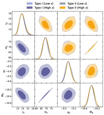
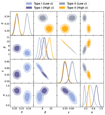
Figure 1: One-dimensional marginalized distributions and two-dimensional contours at 1$\sigma$ and 2$\sigma$ CLs of the Type I and Type II relations from low-redshift and high-redshift quasars.

The best-fitting values with uncertainties are obtained by using the Markov Chain Monte Carlo (MCMC) method, which is available via the $emcee$ package in Python 3.7 (Foreman-Mackey et al., 2013). Table 1 and Figure 1 show the marginalized results and the probability contour plots, respectively. From them, we obtain the following main results:

• For the standard relation, the constraints from the low-redshift and high-redshift data on all the parameters are inconsistent. This agrees with the conclusion obtained in (Li et al., 2022).

• For the redshift-evolutionary relations, the cosmographic parameters ($t_{0}$, $H_{0}$ and $q_{0}$) and the absolute magnitude ($M_{B}$) are consistent in two different redshift ranges. However, the values of the relation coefficients ($\beta$, $\gamma$ and $\alpha$) and the intrinsic dispersion ($\delta$) from the low-redshift and high-redshift data respectively are discrepant. This is similar to what obtained in the standard relation case.

• The redshift-evolutionary coefficient $\alpha$ deviates from zero at more than $2\sigma$, which implies that the observational data support a redshift-dependent relation. Furthermore, the redshift-evolutionary character is more apparent in the Type I relation than that in the Type II case.

Therefore, the redshift-evolutionary $L_{X}$-$L_{UV}$ relations are favored as opposed to the standard one since consistent PAge parameters can be obtained in the redshift-evolutionary relations and the value of $\alpha$ deviates from zero at more than $2\sigma$.

4 Simultaneous Constraints

To further compare the three different $L_{X}$-$L_{UV}$ relations, we will use all $H(z)$, SNe Ia and quasar data to constrain the PAge parameters ($t_{0}$, $H_{0}$ and $q_{0}$), the absolute magnitude ($M_{B}$), the coefficients of the relations ($\beta$, $\gamma$ and $\alpha$) and the intrinsic dispersion ($\delta$) simultaneously. We will utilize the Akaike information criterion (AIC) (Akaike, 1974, 1981) and the Bayes information criterion (BIC) (Schwarz, 1978) to find the relation favored by the observations. The AIC and BIC are defined, respectively, as

$$\mathrm{AIC} = 2p-2\ln\mathcal{L}_{\rm max}\,,$$ (16)

$$\mathrm{BIC} = p\ln N-2\ln\mathcal{L}_{\rm max}\,,$$ (17)

where $\mathcal{L}_{\rm max}$ is the maximum value of the likelihood function, $p$ represents the number of free parameters and $N$ is the number of data. We calculate $\Delta$AIC(BIC) of the three relations, which denotes the difference in the AIC(BIC) of a given relation relative to the reference relation (the Type I relation ), i.e., $\rm\Delta AIC(BIC)=AIC(BIC)-AIC_{ref}(BIC_{ref})$, for the relation comparison. If $0<\Delta\mathrm{AIC(BIC)}\leq 2$, it is difficult to single out a better relation. If $2<\Delta\mathrm{AIC(BIC)}\leq 6$ we have mild evidence against the given relation, and we have strong evidence against the given relation if $\Delta\mathrm{AIC(BIC)}>6$. The parameter values and $\Delta$AIC(BIC) obtained from MCMC are summarized in Table 2, and the posterior distribution contours are shown in Figure 2. In the last column of Table 2, the constraints on the PAge parameters and the absolute magnitude obtained from data without the quasars are also displayed in order to assess the influence of the quasars.

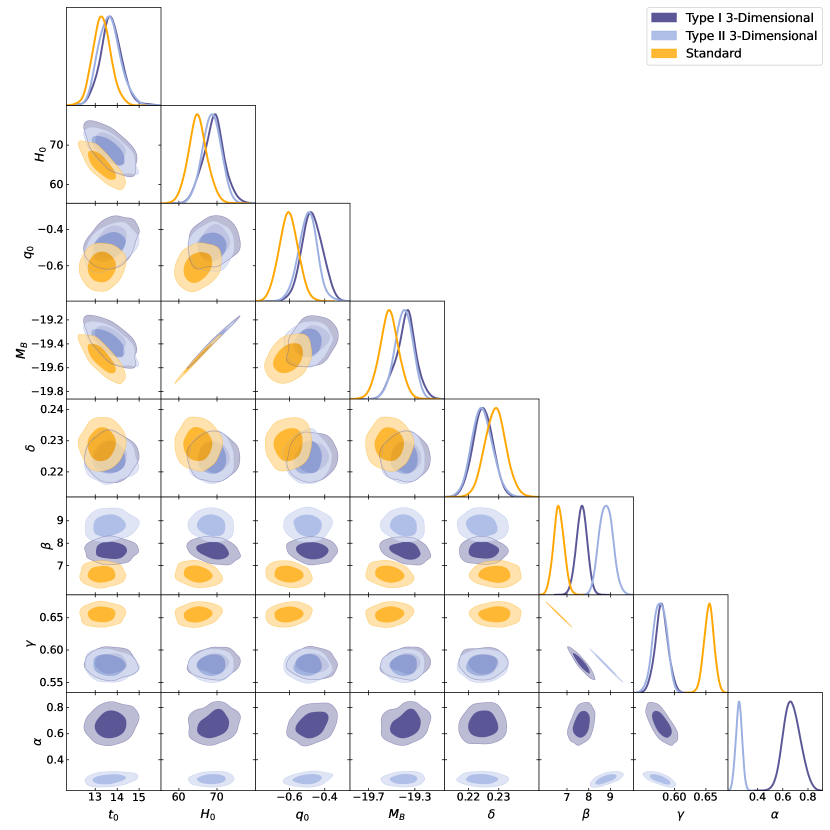
Figure 2: The marginalized posterior distributions and two-dimensional contours at 1$\sigma$ and 2$\sigma$ CLs from $H(z)$+SNe Ia+quasar data in the PAge approximation.

Table 2: The marginalized results with 1$\sigma$ CL for three different luminosity relations from $H(z)$+SNe Ia+quasar data in the PAge approximation. The results from data without the quasars are also displayed for a comparison.

	Type I Three-Dimensional	Type II Three-Dimensional	Standard	Without quasars
$t_{0}$	$13.72\pm 0.50$	$13.65^{+0.44}_{-0.56}$	$13.30\pm 0.43$	$13.67^{+0.44}_{-0.53}$
$H_{0}$	$69.1\pm 2.8$	$68.6\pm 2.5$	$65.0\pm 2.5$	$69.4\pm 2.7$
$q_{0}$	$-0.471\pm 0.059$	$-0.496\pm 0.055$	$-0.606\pm 0.054$	$-0.471\pm 0.057$
$M_{B}$	$-19.377^{+0.092}_{-0.079}$	$-19.395\pm 0.078$	$-19.521\pm 0.084$	$-19.369^{+0.091}_{-0.077}$
$\delta$	$0.2248\pm 0.0033$	$0.2245^{+0.0032}_{-0.0037}$	$0.2289\pm 0.0035$	$-$
$\beta$	$7.68\pm 0.25$	$8.80\pm 0.32$	$6.62\pm 0.24$	$-$
$\gamma$	$0.579\pm 0.010$	$0.577\pm 0.011$	$0.655\pm 0.008$	$-$
$\alpha$	$0.672^{+0.063}_{-0.073}$	$0.252\pm 0.025$	$-$	$-$
$-2\ln\mathcal{L}_{\rm max}$	$1246.550$	$1250.415$	$1350.201$	$-$
$\Delta$AIC	$-$	$3.865$	$101.651$	$-$
$\Delta$BIC	$-$	$3.865$	$95.346$	$-$

Note. — The unit of $t_{0}$ is Gyr and $H_{0}$ is ${\rm km\;s^{-1}\;Mpc^{-1}}$.

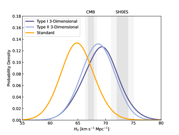
Figure 3: Probability density of Hubble constant $H_{0}$ for different luminosity relations. The gray shades represent the results from the Planck 2018 CMB observations ($H_{0}=67.4\pm 0.5\;{\rm km\;s^{-1}\;Mpc^{-1}}$ (Planck Collaboration et al., 2020)) and the SH0ES ($H_{0}=73.04\pm 1.04\;{\rm km\;s^{-1}\;Mpc^{-1}}$) (Riess et al., 2022) at 68% CL (dark gray) and 95% CL (light gray).

One can see that the constraints on the PAge parameters ($H_{0}$, $t_{0}$ and $q_{0}$) and the absolute magnitude $M_{B}$ from $H(z)$+SNe Ia+quasars with the Type I relation are well consistent with those from data without the quasars. The values of the PAge parameters and the absolute magnitude are compatible with each other for the Type I and Type II relations, while they apparently deviate for the standard relation. The values of $t_{0}$ for the Type I and Type II relations are more comparable with the result from the Planck 2018 CMB observations ($t_{0}=13.801\pm 0.024$ Gyr) (Planck Collaboration et al., 2020) than those for the standard relation. The deceleration parameter $q_{0}$ for the Type I and Type II relations is slightly larger than that in the $\Lambda$CDM model ($q_{0}=3\Omega_{m0}/2-1=-0.528\pm 0.011$) from the Planck 2018 CMB observations (Planck Collaboration et al., 2020), while its value for the standard relation is smaller than $q_{0}=-0.528\pm 0.011$. Furthermore, we find that the value of the Hubble constant $H_{0}$ for the Type I and Type II relations is lager than that for the standard relation, and locates in the region between the Planck 2018 CMB observations (Planck Collaboration et al., 2020) and the local distance ladders from SH0ES (Riess et al., 2022), which can be seen in Figure 3, where the values of $H_{0}$ from the quasars+$H(z)$+SNe Ia, the Planck 2018, and the SH0ES are shown.

The intrinsic dispersion $\delta$ and the relation coefficient $\gamma$ have almost the same values in the Type I and Type II relations, which are larger than those obtained in the standard relation. The value of $\gamma$ in the two three-dimensional relations is consistent with $\gamma=0.586\pm 0.061$ obtained through the narrow redshift bin method (Lusso et al., 2020). For the relation coefficient $\beta$, the Type II relation has the maximum value and the standard relation has the minimum one. The deviations of $\beta$ among three different relations are of more than $2\sigma$. The observations favor strongly the redshift-evolutionary relations since $\alpha=0$ is ruled out at more than $3\sigma$. The value of $\alpha$ in the Type I relation is apparently larger than that in the Type II relation, which indicates that the redshift-evolutionary character in the Type I relation is more apparent than that in the Type II relation. The $\alpha$ value in the Type I relation is comparable with $\alpha=0.580^{+0.084}_{-0.099}$ obtained in the $\Lambda$CDM model (Wang et al., 2022). From Table 2, we find that the Type I three-dimensional relation has the minimum AIC(BIC). The $\Delta$AIC(BIC) of the standard relation is much larger than 6, which indicates that we have strong evidence against it. The $\Delta$AIC(BIC) of the Type II three-dimensional relation is 3.865. Thus, the Type I three-dimensional relation has a slight advantage.

5 Selection effects

To check whether our result that the redshift-evolutionary relation is favored by the observations is caused by the selection effects involved in the measurement process, we follow the method given in (Li, 2007; Singh et al., 2022) and use firstly Monte Carlo simulations to simulate a realistic population of quasars as a function of redshift. Since the 2421 quasar data points satisfy the Gamma distribution in the $z$ space (Lusso et al., 2020), we use this Gamma distribution to generate the redshift distribution of the simulated data. At redshift $z$, the value of $\log(F_{UV})$ is assumed to satisfy the Gaussian distribution shown in Eq. (8) with the mean value and the standard deviation being $-27.503$ and $0.488$, respectively, which are obtained from the real data. We further assume that the error ($\sigma_{{UV}}$) of $\log(F_{UV})$ satisfies the lognormal distribution and find, by using the real data, the mean value and the standard deviation being $-4.342$ and $0.566$ respectively. Since the real data show a correlation between $z$ and $\log(F_{UV})$ with the correlation coefficient being $\rho=-0.255$, we also consider this correlation when generating the ($z,\log(F_{UV})$) pair. Then, we remove the simulated data below the UV flux limit, i.e., the minimum observable flux $\log(F_{UV})_{min}=-28.759$. The flux limit reflects the detection capability of the instrument, and quasars are unobservable by current detectors if their $\log(F_{UV})$ are less than $\log({F_{UV}})_{min}$. For any pair of ($z,\log(F_{UV})$), we generate $\log(F_{X})$ by assuming its distribution function to be $f(\log(F_{X}))=\frac{1}{\sqrt{2\pi}\delta}\exp\left\{-\frac{[\log(F_{X})-\Phi(\log(F_{UV}),d_{L}({\bf p}))]^{2}}{2\delta^{2}}\right\}$ and the luminosity relation to be the standard $L_{X}$-$L_{UV}$ relation, where the intrinsic dispersion $\delta$, the relation coefficients and the PAge parameters ${\bf p}$ are taken as fixed values shown in the third column of Table 2.

With the above approach, we generate 2500 quasars. Using these simulated data, we can fit the intrinsic dispersion and the Type I relation coefficients with the fixed PAge parameters. This process is repeated twenty times, resulting in the average values of the intrinsic dispersion and the relation coefficients to be: $\bar{\delta}=0.2254\pm 0.0032$, $\bar{\beta}=6.46\pm 0.21$, $\bar{\gamma}=0.657\pm 0.009$, and $\bar{\alpha}=0.050\pm 0.054$. Apparently, they have slightly smaller errors than those shown in the first column of Table 2. This is because the errors of the PAge parameters are ignored when fitting the intrinsic dispersion and the relation coefficients from the simulated data. In Figure 4, the twenty values of the relation coefficient $\alpha$ from the simulated data are displayed to compare with $\alpha=0$ used in the simulation. It is easy to see that $\alpha=0$ is included in the 1$\sigma$ CL of the average value of twenty $\alpha$. Comparing $\bar{\alpha}=0.050\pm 0.054$ with $\alpha=0.672^{+0.063}_{-0.073}$ shown in Table 2, we find that the selection effects are ruled out as the possible cause of redshift-evolution of the $L_{X}$-$L_{UV}$ relation.

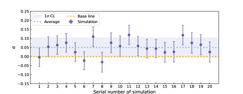
Figure 4: The twenty results of relation coefficient $\alpha$ from the simulated data. The orange base line shows the $\alpha=0$ line. The blue dotted line represents the best fitting value of the average value $\bar{\alpha}$ and the blue shaded area corresponds to the $1\sigma$ CL of $\bar{\alpha}$.

6 Conclusions

Recently, a three-dimensional and redshift-evolutionary $L_{X}$-$L_{UV}$ relation of quasars was constructed from the Gaussian copula (Wang et al., 2022). In this paper, we compare, by using the observational data from quasars, the Hubble parameter measurements and the Pantheon+ SNe Ia sample, this redshift-evolutionary $L_{X}$-$L_{UV}$ relation with another redshift-evolutionary $L_{X}$-$L_{UV}$ relation constructed by considering a redshift dependent correction to the luminosities of quasars and the standard $L_{X}$-$L_{UV}$ relation. We do not assume any cosmological model but use the PAge approximation to describe the cosmic background evolution. The quasar data are divided into the low-redshift part and the high-redshift one. The low-redshift and high-redshift data are then utilized respectively to constrain the relation coefficients, the SNe Ia absolute magnitude, the intrinsic dispersion of quasars and the PAge parameters. For the two redshift-evolutionary relations, we find that the low-redshift and high-redshift data can give consistent results on the PAge parameters and the absolute magnitude of the SNe Ia. While, the values of the relation coefficients respectively from the low-redshift and high-redshift data are discrepant. If the standard relation is considered, all the results from the low-redshift and high-redshift data are incomparable. Furthermore, we find that the observations favor the redshift-evolutionary relations at more than $2\sigma$. Thus, the redshift-evolutionary relations of quasars are favored by the observations as opposed to the standard one.

To further compare three different relations, we use the quasar, $H(z)$ and SNe Ia data to simultaneously constrain the PAge parameters, the intrinsic dispersion, the relation coefficients and the absolute magnitude of the SNe Ia. We find that the constraints obtained with the two redshift-evolutionary relations on the PAge parameters, the absolute magnitude, the intrinsic dispersion and the relation coefficient $\gamma$ are well consistent with each other, but they deviate significantly from those obtained in the standard relation. For the relation coefficient $\beta$, different relations lead to different values and the deviations between them are more than $2\sigma$. The observations favor strongly the redshift-evolutionary relations since $\alpha=0$ is ruled out more than $3\sigma$. According to the AIC and BIC, we find that there is strong evidence against the standard relation and mild evidence against the redshift-evolutionary relation obtained by considering a correction to luminosities of quasars. We also confirm that the redshift-evolution of the $L_{X}$-$L_{UV}$ relation can not be caused by the selection effects. Therefore, we can conclude that among the three different $L_{X}$-$L_{UV}$ relations the redshift-evolutionary relation from copula is the most favored one.

Appendix A PAge Approximation

When constructing the PAge approximation, two underlying assumptions are used (Huang, 2020):

• The product of the Hubble expansion rate $H(t)$ and the cosmic time $t$ can be approximated as a quadratic function of $t$.

• The universe is matter-dominated at redshift $z\gg 1$ with the radiation-dominant epoch, which occurs shortly before the matter domination, being disregarded.

Thus, expanding $H(t)t$ at the cosmic age $t_{0}$ to the second order, we can obtain

$$H(t)t = p_{\rm age}-(1-p_{\rm age}-p_{\rm age}q_{0})(t_{0}-t)H_{0}$$ (A1)

$$- \left(1+q_{0}-\frac{p_{\rm age}}{2}(2+3q_{0}+j_{0})\right)(t_{0}-t)^{2}H_{0}^{2}+\mathcal{O}\left((t_{0}-t)^{3}\right),$$

where $p_{\rm age}\equiv H_{0}t_{0}$, $q_{0}$ is the present deceleration parameter, $j_{0}$ is the present jerk parameter, and

$$a(t)=1-H_{0}(t_{0}-t)-\frac{1}{2}H_{0}^{2}q_{0}(t_{0}-t)^{2}-\frac{1}{6}H_{0}^{3}j_{0}(t_{0}-t)^{3}+\mathcal{O}\left((t_{0}-t)^{4}\right)$$ (A2)

has been used.

In order to achieve a highly precise approximation at high redshift, we now consider the second assumption. When the redshift becomes very high ($z\gg 1$) as the time tends to zero ($t\to 0$), the universe is dominated by matter. Thus, the Hubble parameter can be expressed as $H(t)=\frac{2}{3t}$ at $t\to 0$, which means $\lim\limits_{t\to 0}H(t)t=\frac{2}{3}$. To ensure that Eq. (A1) satisfies the condition $\lim\limits_{t\to 0}H(t)t=\frac{2}{3}$, we modify the coefficient of the $(t_{0}-t)^{2}$ term and then obtain

$$H(t)t = p_{age}-(1-p_{\rm age}-p_{\rm age}q_{0})(t_{0}-t)H_{0}$$ (A3)

$$-\left(1+q_{0}-\frac{2}{3p_{\rm age}^{2}}\right)(t_{0}-t)^{2}H_{0}^{2}.$$

Performing a mathematical transformation, one has

$$\frac{H(t)}{H_{0}}=1+\frac{2}{3}\left(1-\eta\frac{H_{0}t}{p_{\rm age}}\right)\left(\frac{1}{H_{0}t}-\frac{1}{p_{\rm age}}\right),$$ (A4)

which is the common form of the PAge approximation. Here $\eta\equiv 1-\frac{3}{2}p_{\rm age}^{2}(1+q_{0})$.

References

- Akaike (1974) Akaike, H. 1974, IEEE Transactions on Automatic Control, 19, 716, doi: https://ui.adsabs.harvard.edu/abs/1974ITAC…19..716A
- Akaike (1981) Akaike, H. 1981, Journal of Econometrics, 16, 3, doi: https://doi.org/10.1016/0304-4076(81)90071-3
- Bañados et al. (2018) Bañados, E., Venemans, B. P., Mazzucchelli, C., et al. 2018, Nature, 553, 473, doi: 10.1038/nature25180
- Baldwin (1977) Baldwin, J. A. 1977, ApJ, 214, 679, doi: 10.1086/155294
- Banerjee et al. (2021) Banerjee, A., Ó Colgáin, E., Sasaki, M., Sheikh-Jabbari, M. M., & Yang, T. 2021, Physics Letters B, 818, 136366, doi: 10.1016/j.physletb.2021.136366
- Bargiacchi et al. (2022) Bargiacchi, G., Benetti, M., Capozziello, S., et al. 2022, Mon. Not. R. Astron. Soc., 515, 1795, doi: 10.1093/mnras/stac1941
- Bargiacchi et al. (2021) Bargiacchi, G., Risaliti, G., Benetti, M., et al. 2021, Astron. Astrophys., 649, A65, doi: 10.1051/0004-6361/202140386
- Brout et al. (2022) Brout, D., Scolnic, D., Popovic, B., et al. 2022, ApJ, 938, 110, doi: 10.3847/1538-4357/ac8e04
- Cai et al. (2022a) Cai, R.-G., Guo, Z.-K., Wang, S.-J., Yu, W.-W., & Zhou, Y. 2022a, Phys. Rev. D, 106, 063519, doi: 10.1103/PhysRevD.106.063519
- Cai et al. (2022b) —. 2022b, Phys. Rev. D, 105, L021301, doi: 10.1103/PhysRevD.105.L021301
- Cai et al. (2022c) —. 2022c, Phys. Rev. D, 106, 063519, doi: 10.1103/PhysRevD.106.063519
- Cao et al. (2021) Cao, S., Ryan, J., Khadka, N., & Ratra, B. 2021, Mon. Not. R. Astron. Soc., 501, 1520, doi: 10.1093/mnras/staa3748
- Chen & Ratra (2003) Chen, G., & Ratra, B. 2003, ApJ, 582, 586, doi: 10.1086/344786
- D’Agostini (2005) D’Agostini, G. 2005, arXiv e-prints, physics/0511182, doi: 10.48550/arXiv.physics/0511182
- Dainotti et al. (2022) Dainotti, M. G., Bargiacchi, G., Lenart, A. Ł., et al. 2022, ApJ, 931, 106, doi: 10.3847/1538-4357/ac6593
- Efron & Petrosian (1992) Efron, B., & Petrosian, V. 1992, ApJ, 399, 345, doi: 10.1086/171931
- Foreman-Mackey et al. (2013) Foreman-Mackey, D., Hogg, D. W., Lang, D., & Goodman, J. 2013, J Publications of the Astronomical Society of the Pacific, 125, 306, doi: 10.1086/670067
- Huang et al. (2021) Huang, L., Huang, Z., Luo, X., He, X., & Fang, Y. 2021, Phys. Rev. D, 103, 123521, doi: 10.1103/PhysRevD.103.123521
- Huang et al. (2022) Huang, L., Huang, Z., Zhou, H., & Li, Z. 2022, Science China Physics, Mechanics, and Astronomy, 65, 239512, doi: 10.1007/s11433-021-1838-1
- Huang (2020) Huang, Z. 2020, Astrophys. J. Lett., 892, L28, doi: 10.3847/2041-8213/ab8011
- Khadka & Ratra (2020a) Khadka, N., & Ratra, B. 2020a, Mon. Not. R. Astron. Soc., 492, 4456, doi: 10.1093/mnras/staa101
- Khadka & Ratra (2020b) —. 2020b, Mon. Not. R. Astron. Soc., 497, 263, doi: 10.1093/mnras/staa1855
- Khadka & Ratra (2021) —. 2021, Mon. Not. R. Astron. Soc., 502, 6140, doi: 10.1093/mnras/stab486
- Khadka & Ratra (2022) —. 2022, Mon. Not. R. Astron. Soc., 510, 2753, doi: 10.1093/mnras/stab3678
- Khadka et al. (2022) Khadka, N., Zajaček, M., Prince, R., et al. 2022, arXiv e-prints, arXiv:2212.10483, doi: 10.48550/arXiv.2212.10483
- La Franca et al. (2014) La Franca, F., Bianchi, S., Ponti, G., Branchini, E., & Matt, G. 2014, Astrophys. J. Lett., 787, L12, doi: 10.1088/2041-8205/787/1/L12
- Lenart et al. (2023) Lenart, A. Ł., Bargiacchi, G., Dainotti, M. G., Nagataki, S., & Capozziello, S. 2023, Astrophys. J. Suppl., 264, 46, doi: 10.3847/1538-4365/aca404
- Li (2007) Li, L.-X. 2007, MNRAS, 379, L55. doi: 10.1111/j.1745-3933.2007.00333.x
- Li et al. (2021) Li, X., Keeley, R. E., Shafieloo, A., et al. 2021, Mon. Not. R. Astron. Soc., 507, 919, doi: 10.1093/mnras/stab2154
- Li et al. (2022) Li, Z., Huang, L., & Wang, J. 2022, Mon. Not. R. Astron. Soc., 517, 1901, doi: 10.1093/mnras/stac2735
- Lian et al. (2021) Lian, Y., Cao, S., Biesiada, M., et al. 2021, Mon. Not. R. Astron. Soc., 505, 2111, doi: 10.1093/mnras/stab1373
- Liu et al. (2023) Liu, Y., Yu, H., & Wu, P. 2023, ApJ, 946, L49, doi: 10.3847/2041-8213/acc650
- Luo et al. (2020) Luo, X., Huang, Z., Qian, Q., & Huang, L. 2020, ApJ, 905, 53, doi: 10.3847/1538-4357/abc25f
- Lusso et al. (2019) Lusso, E., Piedipalumbo, E., Risaliti, G., et al. 2019, Astron. Astrophys., 628, L4, doi: 10.1051/0004-6361/201936223
- Lusso & Risaliti (2016) Lusso, E., & Risaliti, G. 2016, ApJ, 819, 154, doi: 10.3847/0004-637X/819/2/154
- Lusso et al. (2020) Lusso, E., Risaliti, G., Nardini, E., et al. 2020, Astron. Astrophys., 642, A150, doi: 10.1051/0004-6361/202038899
- Lyke et al. (2020) Lyke, B. W., Higley, A. N., McLane, J. N., et al. 2020, Astrophys. J. Suppl., 250, 8, doi: 10.3847/1538-4365/aba623
- Mehrabi & Basilakos (2020) Mehrabi, A., & Basilakos, S. 2020, European Physical Journal C, 80, 632, doi: 10.1140/epjc/s10052-020-8221-2
- Moresco (2015) Moresco, M. 2015, Mon. Not. R. Astron. Soc., 450, L16, doi: 10.1093/mnrasl/slv037
- Moresco et al. (2020) Moresco, M., Jimenez, R., Verde, L., Cimatti, A., & Pozzetti, L. 2020, ApJ, 898, 82, doi: 10.3847/1538-4357/ab9eb0
- Moresco et al. (2012) Moresco, M., Cimatti, A., Jimenez, R., et al. 2012, J. Cosmol. Astropart. Phys., 2012, 006, doi: 10.1088/1475-7516/2012/08/006
- Moresco et al. (2016) Moresco, M., Pozzetti, L., Cimatti, A., et al. 2016, J. Cosmol. Astropart. Phys., 2016, 014, doi: 10.1088/1475-7516/2016/05/014
- Mortlock et al. (2011) Mortlock, D. J., Warren, S. J., Venemans, B. P., et al. 2011, Nature, 474, 616, doi: 10.1038/nature10159
- Paragi et al. (1999) Paragi, Z., Frey, S., Gurvits, L. I., et al. 1999, Astron. Astrophys., 344, 51, doi: 10.48550/arXiv.astro-ph/9901396
- Petrosian et al. (2022) Petrosian, V., Singal, J., & Mutchnick, S. 2022, Astrophys. J. Lett., 935, L19, doi: 10.3847/2041-8213/ac85ac
- Planck Collaboration et al. (2020) Planck Collaboration, Aghanim, N., Akrami, Y., et al. 2020, Astron. Astrophys., 641, A6, doi: 10.1051/0004-6361/201833910
- Riess et al. (2022) Riess, A. G., Yuan, W., Macri, L. M., et al. 2022, Astrophys. J. Lett., 934, L7, doi: 10.3847/2041-8213/ac5c5b
- Risaliti & Lusso (2015) Risaliti, G., & Lusso, E. 2015, ApJ, 815, 33, doi: 10.1088/0004-637X/815/1/33
- Risaliti & Lusso (2019) —. 2019, Nature Astronomy, 3, 272, doi: 10.1038/s41550-018-0657-z
- Sacchi et al. (2022) Sacchi, A., Risaliti, G., Signorini, M., et al. 2022, Astron. Astrophys., 663, L7, doi: 10.1051/0004-6361/202243411
- Schwarz (1978) Schwarz, G. 1978, Annals of Statistics, 6, 461, doi: https://ui.adsabs.harvard.edu/abs/1978AnSta…6..461S
- Singh et al. (2022) Singh, M., Singh, D., Lal Pandey, K., et al. 2022, arXiv:2211.11667. doi: 10.48550/arXiv.2211.11667
- Velten & Gomes (2020) Velten, H., & Gomes, S. 2020, Phys. Rev. D, 101, 043502, doi: 10.1103/PhysRevD.101.043502
- Wang et al. (2022) Wang, B., Liu, Y., Yuan, Z., et al. 2022, ApJ, 940, 174, doi: 10.3847/1538-4357/ac9df8
- Wang et al. (2021) Wang, F., Yang, J., Fan, X., et al. 2021, Astrophys. J. Lett., 907, L1, doi: 10.3847/2041-8213/abd8c6
- Wang et al. (2014) Wang, J.-M., Du, P., Hu, C., et al. 2014, ApJ, 793, 108, doi: 10.1088/0004-637X/793/2/108
- Watson et al. (2011) Watson, D., Denney, K. D., Vestergaard, M., & Davis, T. M. 2011, Astrophys. J. Lett., 740, L49, doi: 10.1088/2041-8205/740/2/L49
- Wei & Melia (2020) Wei, J.-J., & Melia, F. 2020, ApJ, 888, 99, doi: 10.3847/1538-4357/ab5e7d
- Yang et al. (2020) Yang, T., Banerjee, A., & Ó Colgáin, E. 2020, Phys. Rev. D, 102, 123532, doi: 10.1103/PhysRevD.102.123532