Twisted Yang-Baxter sets, cohomology theory, and application to knots

Abstract.

In this article, we introduce a notion of twisted set-theoretic Yang-Baxter solution, which is a triplet $(X,f,R)$, where $(X,R)$ is a Yang-Baxter set and $f:X\to X$ is an automorphism of $(X,R)$. We present a cohomology theory for it, and use cocycles of twisted biquandles in amalgamation with Alexander numbering to construct state-sum invariant of knots and knotted surfaces. Additionally, we introduce a twisted version of cohomology theory for Yang-Baxter sets and give applications to knot theory.

1. Introduction

The Yang-Baxter equation first appeared in theoretical physics independently in the work of Yang [24]and Baxter [3]. Since then it has played an important role in the theory of quantum groups, braided categories and knot theory. A Yang-Baxter set is a pair $(X,R)$, where $X$ is a set and $R:X\times X\rightarrow X\times X$ is an invertible map satisfying the equation

$$(R\times\mathrm{id}_{X})(\mathrm{id}_{X}\times R)(R\times\mathrm{id}_{X})=(\mathrm{id}_{X}\times R)(R\times\mathrm{id}_{X})(\mathrm{id}_{X}\times R),$$

where $\mathrm{id}_{X}:X\rightarrow X$ is the identity map. Solutions to the Yang-Baxter equation allow constructions of invariants of knots [23, 13]. For example, a certain solution to the Yang-Baxter equation gives rise to the Jones polynomial [12]. Algebraic knot invariants such as quandles [14, 20], and biquandles [19, 16] are solutions of the Yang-Baxter equation. Using the concept of Yang-Baxter coloring of cubical complexes, Carter-Elhamdadi-Saito [5] developed a homology theory for the Yang-Baxter equation, and used cocycles to define knot invariants via biquandle colorings of knot diagrams by biquandles and a state-sum formulation. In [15], biquandle cocycles are used to define state-sum invariant for knotted surfaces. Przytycki [21] used a graphical approach to define a homology theory for the Yang-Baxter equation, and it is proved in [22] that both the approaches give the same homology theory. In [9], an $S$-homology theory is introduced for virtual biquandles which in augmentation with biquandle $2$-cocycles were used to detect non-classicality of virtual knots and links. A virtual biquandle [18] is a biquandle $(X,R)$ along with an automorphism $f:X\to X$. Recently, in [10], it is shown that for a given virtual link $L$, the set of colorings of $L$ by a virtual biquandle $(X,f,R)$ (see [18]) is in bijective correspondence with the set of colorings of $L$ by the biquandle $(X,VR)$, where $VR$ is a new Yang-Baxter operator constructed from $R$ and $f$. In this article, we refer to virtual biquandles as twisted biquandles.

In this article, we introduce a notion of twisted set-theoretic Yang-Baxter solution, which is a triplet $(X,f,R)$, where $(X,R)$ is a Yang-Baxter set and $f:X\to X$ an automorphism of $(X,R)$. For instance, twisted biquandles are such examples. Using a graphical approach, we introduce a (co)homology theory for it, and use cocycles of twisted biquandles in amalgamation with Alexander numbering to construct state-sum invariant of knots and knotted surfaces. Furthermore, we also introduce a twisted version of (co)homology theory of Yang-Baxter set and give its applications to knots.

Throughout the paper we refer to knots and links by the generic term “knots”.

The article is organized as follows. In Section 2 we review the basics of the Yang-Baxter equation and Yang-Baxter homology focusing on the graphical approach [21]. Section 3 introduces twisted set-theoretic Yang-Baxter solutions. In Section 4 we introduce (co)homology theory for twisted Yang-Baxter sets and twisted biquandles. Section 5 deals with extension theory of the twisted Yang-Baxter sets using cocycles. In Section 6, using $2$-cocycles for twisted biquandles in amalgamation with Alexander numbering of knots we introduce a state-sum knot invariant. Analogous approach is used in Section 7 to define state-sum invariant for knotted surfaces. In Section 8, we note that one can analogously define state sum invariants for knots on compact oriented surfaces and broken surface diagrams in orientable compact $3$-manifolds. Furthermore, we introduce a twisted version of Yang-Baxter (co)homology theory which is a generalization of twisted quandle (co)homology theory [4] in two different ways.

2. Preliminaries

A precubical set is a graded set $P=(P_{n})_{n\geq 0}$ with boundary operators $\partial^{k}_{i}:P_{n}\to P_{n-1}$ $(n>0,~{}k=0,1,~{}i=1,\ldots,n)$ satisfying the equations $\partial^{k}_{i}\circ\partial_{j}^{l}=\partial_{j-1}^{l}\circ\partial_{i}^{k}$ $(k,l=0,1,~{}i<j)$.

2.1. Yang-Baxter solutions

Let $X$ be a non-empty set and $R:X\times X\to X\times X$ an invertible map, satisfying the following equation

$$(R\times\mathrm{id}_{X})(\mathrm{id}_{X}\times R)(R\times\mathrm{id}_{X})=(\mathrm{id}_{X}\times R)(R\times\mathrm{id}_{X})(\mathrm{id}_{X}\times R),$$

known as set-theoretic Yang-Baxter equation, where $\mathrm{id}_{X}$ denotes the identity map on $X$. Then $R$ is termed as set-theoretic Yang-Baxter operator and the pair $(X,R)$ is said to be set-theoretic Yang-Baxter solution. Sometimes for brevity, we call $(X,R)$ as Yang-Baxter set.

We denote the components of $R$ by $R_{1}$ and $R_{2}$, that is, $R(x_{1},x_{2})=\big{(}R_{1}(x_{1},x_{2}),R_{2}(x_{1},x_{2})\big{)}$ for $x_{1},x_{2}\in X$. Moreover, $\mkern 1.5mu\overline{\mkern-1.5muR\mkern-1.5mu}\mkern 1.5mu$ denotes the inverse of $R$, and $\mkern 1.5mu\overline{\mkern-1.5muR_{1}\mkern-1.5mu}\mkern 1.5mu$ and $\mkern 1.5mu\overline{\mkern-1.5muR_{2}\mkern-1.5mu}\mkern 1.5mu$ are its components.

A Yang-Baxter set $(X,R)$ is called a birack if

1. the map $R_{1}$ is left-invertible, that is, for any $x,z\in X$, there is a unique $y\in X$ such that $R_{1}(x,y)=z$;

2. the map $R_{2}$ is right-invertible, that is, for any $y,w\in X$, there is unique $x\in X$ such that $R_{2}(x,y)=w$.

A biquandle is a birack $(X,R)$ satisfying the type I condition, that is, for a given $a\in X$ there exists a unique $x\in X$ such that $R(x,a)=(x,a)$. Note that the above condition is equivalent to the following: given an element $a\in X$ there exists a unique $x\in X$ such that $R(a,x)=(a,x)$. For more details, see [2, 11] and [5, Remark 3.3].

Examples.

1. Let $(X,*)$ be a quandle. Then define $R:X\times X\to X\times X$ as $R(x,y)=(y,x*y)$. Then $(X,R)$ is a biquandle.

2. Let $\mathbb{Z}_{n}$ be a cyclic group of order $n$. Define $R:\mathbb{Z}_{n}\times\mathbb{Z}_{n}\to\mathbb{Z}_{n}\times\mathbb{Z}_{n}$ as $R(x,y)=(y+1,x-1)$. Then $(\mathbb{Z}_{n},R)$ is a biquandle.

3. Let $G$ be a group. Define $R,R^{\prime}:G\times G\to G\times G$ as $R(x,y)=(y^{-1},yxy)$ and $R^{\prime}(x,y)=(x^{-1}y^{-1}x,y^{2}x)$. Then $(G,R)$ and $(G,R^{\prime})$ are biquandles and are called Wada biquandles.

4. Let $K$ be a commutative ring with unit $1$. Let $\alpha,\beta$ are units in $K$ such that $(1-\alpha)(1-\beta)=0$. Then $\displaystyle R=\left[\begin{array}[]{cc}1-\alpha&\alpha\\ \beta&1-\beta\end{array}\right]$ makes the ring $K$ into a biquandle and is known as Alexander biquandle.

Definition 2.1.

Let $(X,R)$ be a birack and $f:X\to X$ be an automorphism of $X$, that is, $f$ is a bijection and the following diagram commutes

Then we call $(X,f,R)$ a twisted birack. In the study of virtual knots (see [18]) , $(X,f,R)$ is called a virtual birack.

If in the above definition $(X,R)$ is a biquandle, then $(X,f,R)$ is called twisted biquandle.

2.2. Yang-Baxter (co)homology theory

There are two approaches for homology theory of the set-theoretic Yang-Baxter sets, one is algebraic [5] and the other is graphical [21], and both of them give the yield the same theory [22]. For our purpose we are using the graphical one.

Let $(X,R)$ be a Yang-Baxter set. Let $C_{n}^{\operatorname{YB}}(X)$ be the free abelian group generated by the elements in $X^{n}$. For each $n\geq 1$ define a homomorphism

$$\partial_{n}:C_{n}^{\operatorname{YB}}\to C_{n-1}^{\operatorname{YB}}(X)$$

as follows, $\partial_{n}=\sum_{i=1}^{n}(-1)^{i}\partial_{i,n}$, where $\partial_{i,n}=\partial^{l}_{i,n}-\partial^{r}_{i,n}$. We can interpret the face maps through Figure 1. The maps $d_{i,n}^{l}$ and $d_{i,n}^{r}$ are illustrated in Figure 2 and Figure 3, respectively.

Figure 1. The map $\partial_{i,n}.$

Figure 2. A face map $\partial^{l}_{i,n}.$

Figure 3. A face map $\partial^{r}_{i,n}.$

One can check that the graded set $(X^{n})_{n\geq 0}$ with boundary maps $\partial^{\epsilon}_{i,n}$, where $\epsilon=l,r$, is a precubical set, which implies that $(C_{*}^{\operatorname{YB}}(X),\partial_{n})$ is a chain complex. One can now proceed in the standard way to define homology and cohomology groups.

3. Twisted set-theoretic Yang-Baxter solutions

In this section, we introduce twisted set-theoretic Yang-Baxter solutions and propose its homology theory, which we call twisted set-theoretic Yang-Baxter homology theory.

Definition 3.1.

A twisted set-theoretic Yang-Baxter solution is a triplet $(X,f,R)$, where $(X,R)$ is a Yang-Baxter set and $f:X\to X$ an automorphism of $(X,R)$, that is, $f$ is a bijective map and the following diagram commutes:

For brevity, we call $(X,f,R)$ as a twisted Yang-Baxter set.

If $(X,f,R)$ is a twisted Yang-Baxter set, then following diagrams commute:

A homomorphism from $(X,f,R)$ to $(Y,f^{\prime},R^{\prime})$ is a map $\phi:(X,f,R)\to(Y,f^{\prime},R^{\prime})$ such that the following diagrams commute

A twisted birack (twisted biquandle) $(X,f,R)$ can also be defined as a twisted Yang-Baxter set $(X,f,R)$, where $(X,R)$ is a birack (biquandle).

Let $(X,f,R)$ be a twisted Yang-Baxter set, where $R=(R_{1},R_{2})$. Define a map

$$\mathcal{T}R:X\times X\to X\times X,$$

as

$$\mathcal{T}R(x,y)=(\mathcal{T}R_{1}(x,y),\mathcal{T}R_{2}(x,y)):=(R_{1}(x,f(y)),R_{2}(f^{-1}(x),y)).$$

The map $\mathcal{T}R$ is invertible, where the inverse map $\mkern 1.5mu\overline{\mkern-1.5mu\mathcal{T}R\mkern-1.5mu}\mkern 1.5mu:X\times X\to X\times X$ is

$$\mkern 1.5mu\overline{\mkern-1.5mu\mathcal{T}R\mkern-1.5mu}\mkern 1.5mu(x,y)=\big{(}\mkern 1.5mu\overline{\mkern-1.5muR_{1}\mkern-1.5mu}\mkern 1.5mu(x,f(y)),\mkern 1.5mu\overline{\mkern-1.5muR_{2}\mkern-1.5mu}\mkern 1.5mu(f^{-1}(x),y)\big{)}.$$ (1)

Since, $R$ satisfies the set-theoretic Yang-Baxter equation, for all $a,b,c\in X$, the following equations hold, which we use in the proof of Lemma 3.1.

$$R_{1}\big{(}R_{1}(a,b),R_{1}(R_{2}(a,b),c)\big{)} =R_{1}\big{(}a,R_{1}(b,c)\big{)}$$ (2)

$$R_{2}\big{(}R_{1}(a,b),R_{1}(R_{2}(a,b),c)\big{)} =R_{1}\big{(}R_{2}(a,R_{1}(b,c)),R_{2}(b,c)\big{)}$$ (3)

$$R_{2}\big{(}R_{2}(a,b),c\big{)} =R_{2}\big{(}R_{2}(a,R_{1}(b,c)),R_{2}(b,c)\big{)}$$ (4)

Lemma 3.1.

The map $\mathcal{T}R:X\times X\to X\times X$ satisfies the set-theoretic Yang-Baxter equation, that is,

$$(\mathcal{T}R\times\mathrm{id}_{X})(\mathrm{id}_{X}\times\mathcal{T}R)(\mathcal{T}R\times\mathrm{id}_{X})=(\mathrm{id}_{X}\times\mathcal{T}R)(\mathcal{T}R\times\mathrm{id}_{X})(\mathrm{id}_{X}\times\mathcal{T}R)$$

Proof.

L.H.S=

$$(\mathcal{T}R\times\mathrm{id}_{X})(\mathrm{id}_{X}\times\mathcal{T}R)(\mathcal{T}R\times\mathrm{id}_{X})~{}~{}(x,y,z)= (\mathcal{T}R\times\mathrm{id}_{X})(\mathrm{id}_{X}\times\mathcal{T}R)~{}~{}\big{(}R_{1}(x,f(y)),R_{2}(f^{-1}(x),y),z\big{)}$$

$$= (\mathcal{T}R\times\mathrm{id}_{X})~{}~{}\big{(}R_{1}(x,f(y)),R_{1}(R_{2}(f^{-1}(x),y),f(z)),$$

$$R_{2}(R_{2}(f^{-2}(x),f^{-1}(y),z)\big{)}$$

$$= \big{(}R_{1}\big{(}R_{1}(x,f(y),R_{1}(R_{2}(x,f(y)),f^{2}(z))\big{)},$$

$$R_{2}\big{(}R_{1}(f^{-1}(x),y),R_{1}(R_{2}(f^{-1}(x),y),f(z)\big{)},$$

$$R_{2}(R_{2}(f^{-2}(x),f^{-1}(y),z)\big{)}$$

R.H.S=

$$(\mathrm{id}_{X}\times\mathcal{T}R)(\mathcal{T}R\times\mathrm{id})(\mathrm{id}_{X}\times\mathcal{T}R)~{}~{}(x,y,z)= (\mathrm{id}_{X}\times\mathcal{T}R)(\mathcal{T}R\times\mathrm{id}_{X})~{}~{}\big{(}x,R_{1}(y,f(z)),R_{2}(f^{-1}(y),z)\big{)}$$

$$= (\mathrm{id}_{X}\times\mathcal{T}R)~{}~{}R_{1}\big{(}x,R_{1}(f(y),f^{2}(z)),R_{2}(f^{-1}(x),R_{1}(y,f(z))),$$

$$R_{2}(f^{-1}(y),z)\big{)}$$

$$= \big{(}R_{1}(x,R_{1}(f(y),f^{2}(z))),R_{1}(R_{2}(f^{-1}(x),R_{1}(y,f(z))),R_{2}(y,f(z))\big{)},$$

$$R_{2}(R_{2}(f^{-2}(x),R_{1}(f^{-1}(y),z)),R_{2}(f^{-1}(y),z))\big{)}$$

Now L.H.S=R.H.S, if and only if the following equations hold for all $x,y,z\in X$:

$$R_{1}\big{(}R_{1}(x,f(y),R_{1}(R_{2}(x,f(y)),f^{2}(z))\big{)}=R_{1}\big{(}x,R_{1}(f(y),f^{2}(z))\big{)}$$ (5)

$$R_{2}\big{(}R_{1}(f^{-1}(x),y),R_{1}(R_{2}(f^{-1}(x),y),f(z)\big{)}=R_{1}\big{(}R_{2}(f^{-1}(x),R_{1}(y,f(z))\big{)},R_{2}(y,f(z))\big{)}$$ (6)

$$R_{2}\big{(}R_{2}(f^{-2}(x),f^{-1}(y),z\big{)}=R_{2}\big{(}R_{2}(f^{-2}(x),R_{1}(f^{-1}(y),z)),R_{2}(f^{-1}(y),z)\big{)}$$ (7)

Equation 5 follows from Equation 2 by replacing $a$ with $x$, $b$ with $f(y)$ and $c$ with $f^{2}(z)$. Equation 6 follows from Equation 3 by replacing $a$ with $f^{-1}(x)$, $b$ with $y$ and $c$ with $f(z)$. Equation 7 follows from Equation 4 by replacing $a$ with $f^{-2}(x)$, $b$ with $f^{-1}(y)$ and $c$ with $z$. ∎

Thus, we call $\mathcal{T}R$ the twisted operator on $(X,f,R)$. For a given integer $t$, we define an operator $\mathcal{T}^{t}R:X\times X\to X\times X$ as follows:

$$\mathcal{T}^{t}R(x,y)=(\mathcal{T}^{t}R_{1}(x,y),\mathcal{T}^{t}R_{2}(x,y)):=(R_{1}(x,f^{t}(y)),R_{2}(f^{-t}(x),y)).$$

It is easy to see that for each $t\in\mathbb{Z}$, $(X,f,\mathcal{T}^{t}R)$ is a twisted Yang-Baxter set. Moreover, we note the following result.

Proposition 3.2.

Let $(X,f,R)$ and $(X^{\prime},f^{\prime},R^{\prime})$ be two twisted Yang-Baxter sets. If $(X,f,R)\cong(X^{\prime},f^{\prime},R^{\prime})$, then $(X,f^{\prime},\mathcal{T}^{t}R)\cong(X^{\prime},f^{\prime},\mathcal{T}^{t}R^{\prime})$ for all $t\in\mathbb{Z}$.

Corollary 3.3.

Let $(X,f,R)$ be a twisted Yang-Baxter set, and $\mathcal{T}R$ be the corresponding twisted operator. Then the following holds:

1. $(X,\mathcal{T}R)$ is a Yang-Baxter set.

2. If $(X,f,R)$ is a twisted birack, then $(X,\mathcal{T}R)$ is a birack.

3. If $(X,f,R)$ is a twisted biquandle, then $(X,\mathcal{T}R)$ is a biquandle.

Remark 3.1.

A twisted rack (or twisted quandle) $(X,f,R)$ is a rack (quandle) $\big{(}X,R=(R_{1},R_{2})\big{)}$, where $R_{1}(x,y)=y$ for all $x,y\in X$, with a bijective map $f:X\to X$ such that $(f\times f)\circ R=R\circ(f\times f)$. Now, under the corresponding twisted operator $\mathcal{T}R$, $(X,\mathcal{T}R)$ is not a rack (quandle) unless $f$ is the identity map on $X$.

4. Twisted Yang-Baxter (co)homology theory

Now, we propose a (co)homology theory for twisted Yang-Baxter sets. Let $(X,f,R)$ be a twisted Yang-Baxter set, $(t,m_{1},m_{2})\in\mathbb{Z}^{3}$. For each integer $n>0$, consider the $n$-chain group $C_{n}^{\operatorname{TYB}}(X)$ to be the free abelian group on $X^{n}$, and for $n>1$, the $n$-boundary homomorphism

$$\partial_{n}^{(t,m_{1},m_{2})}:C_{n}^{\operatorname{TYB}}(X)\to C_{n-1}^{\operatorname{TYB}}(X)$$

is defined as

$$\partial_{n}^{(t,m_{1},m_{2})}=\sum_{i=1}^{n}(-1)^{i}\partial^{(t,m_{1},m_{2})}_{i,n}$$

where

$$\partial_{i,n}^{(t,m_{1},m_{2})}=\partial_{i,n}^{l,(t,m_{1})}-\partial_{i,n}^{r,(t,m_{2})}.$$

The face maps $\partial_{i,n}^{l,(t,m_{1})}$ and $\partial_{i,n}^{r,(t,m_{2})}$ are illustrated in Figures 4 and 5.

Figure 4. A face map $\partial^{l,m_{1}}_{i,n}$

Figure 5. A face map $\partial^{r,m_{2}}_{i,n}$

We take $C_{0}^{\operatorname{TYB}}(X)=\{0\}$. It is easy to check that the graded set $(X^{n})_{n\geq 0}$ along with boundary maps $\partial_{i,n}^{l,(t,m_{1})}$ and $\partial_{i,n}^{r,(t,m_{2})}$, is a precubical set, which implies that $C_{*}^{\operatorname{TYB},(t,m_{1},m_{2})}(X):=\big{(}C_{n}^{\operatorname{TYB}}(X),\partial_{n}^{(t,m_{1},m_{2})}\big{)}$ is a chain complex.

Notice that for each $n\geq 0$, $C_{n}^{\operatorname{TYB}}(X)$ is a module over $\mathbb{Z}[T,T^{-1}]$, where for $(x_{1},\ldots,x_{n})\in X^{n}$, the action is $T.(x_{1},\ldots,x_{n})=(f(x_{1}),\ldots,f(x_{n}))$. Furthermore, each chain map $\partial_{n}^{(t,m_{1},m_{2})}:C_{n}^{\operatorname{TYB}}(X)\to C_{n-1}^{\operatorname{TYB}}(X)$ is a $\mathbb{Z}[T,T^{-1}]$-module homomorphism.

As usual, for a given $\mathbb{Z}[T,T^{-1}]$-module $M$, consider the chain and cochain complexes

$$C_{*}^{\operatorname{TYB},(t,m_{1},m_{2})}(X;M)=C_{*}^{\operatorname{TYB},(t,m_{1},m_{2})}(X)\otimes_{\mathbb{Z}[T,T^{-1}]}M, \partial^{(t,m_{1},m_{2})}=\partial^{(t,m_{1},m_{2})}\otimes\mathrm{id}_{M};$$

$$C^{*}_{\operatorname{TYB},(t,m_{1},m_{2})}(X;M)=\operatorname{Hom}_{\mathbb{Z}[T,T^{-1}]}\big{(}C_{*}^{\operatorname{TYB},(t,m_{1},m_{2})}(X),M\big{)} \delta_{(t,m_{1},m_{2})}=\operatorname{Hom}(\partial^{(t,m_{1},m_{2})},\mathrm{id}_{M}).$$

The $n$-th homology and cohomology groups of these complexes are called $t$-$(m_{1},m_{2})$- twisted Yang-Baxter homology group and cohomology group, and are denoted by $H_{*}^{\operatorname{TYB},(t,m_{1},m_{2})}(X;M)$ and $H^{*}_{\operatorname{TYB},(t,m_{1},m_{2})}(X;M)$, respectively. We call the (co)cycles in this homology theory $t$-$(m_{1},m_{2})$-Yang-Baxter $($co$)$cycles.

Definition 4.1.

The (co)homology theory defined above is called the $t$-$(m_{1},m_{2})$-$($co$)$homology theory of the set-theoretic twisted Yang-Baxter set $(X,f,R)$.

Remark 4.1.

From now onward, we will only study the operator $R:X\times X\to X\times X$, that is, we take $t=0$, unless explicitly stated otherwise. However, all the following results throughout the paper also holds for $\mathcal{T}^{t}R:X\times X\to X\times X$ operator, for any $t\in\mathbb{Z}$. Moreover, we drop the notation for $t=0$, for instance, $C_{*}^{\operatorname{TYB},(0,m_{1},m_{2})}(X;M)$ will be denoted by $C_{*}^{\operatorname{TYB},(m_{1},m_{2})}(X;M)$.

Let $(X,f,R)$ be a twisted biquandle. Consider a $\mathbb{Z}[T,T^{-1}]$-submodule $C_{n}^{\operatorname{TD}}(X)$ of $C_{n}^{\operatorname{TYB}}(X)$ defined by

$$C_{n}^{\operatorname{TD}}(X)=\textrm{ span}\{(x_{1},\ldots,x_{n})\in C_{n}^{\operatorname{TYB}}(X)~{}|~{}R(x_{i},x_{i+1})=(x_{i},x_{i+1})\textrm{ for some }i=1,\ldots,n-1\}$$

if $n\geq 2$, otherwise we let $C_{n}^{\operatorname{TD}}(X)=0$.

The following result is easy to prove and we leave it for readers.

Proposition 4.1.

Let $(X,f,R)$ be a twisted biquandle. Then $\partial_{n}^{(m_{1},m_{2})}(C_{n}^{\operatorname{TD}}(X))\subseteq C_{n-1}^{\operatorname{TD}}(X)$ and $(C_{n}^{\operatorname{TD}}(X),\partial_{n}^{(m_{1},m_{2})})$ is a sub-chain complex of $(C_{n}^{\operatorname{TYB}}(X),\partial_{n}^{(m_{1},m_{2})})$.

Consider the quotient chain complex $C_{*}^{\operatorname{TBQ},(m_{1},m_{2})}(X)=(C_{n}^{\operatorname{TBQ}},\partial_{n}^{(m_{1},m_{2})})$, where $C_{n}^{\operatorname{TBQ}}(X)=C_{n}^{\operatorname{TYB}}(X)/C_{n}^{\operatorname{TD}}(X)$, and $\partial_{n}^{(m_{1},m_{2})}$ is the induced homomorphism.

For a $\mathbb{Z}[T,T^{-1}]$-module $M$, define the chain and cochain complexes $C_{*}^{\operatorname{TBQ},(m_{1},m_{2})}(X;M)=\big{(}C_{n}^{\operatorname{TBQ}}(X;M),\partial_{n}^{(m_{1},m_{2})}\big{)}$ and $C^{*}_{\operatorname{TBQ},(m_{1},m_{2})}(X;M)=(C^{n}_{\operatorname{TBQ}}(X;M),\delta_{(m_{1},m_{2})}^{n})$, where

$$C_{n}^{\operatorname{TBQ}}(X;M) =C_{n}^{\operatorname{TBQ}}(X)\otimes_{\mathbb{Z}[T,T^{-1}]}M, \partial_{n}^{(m_{1},m_{2})}=\partial_{n}^{(m_{1},m_{2})}\otimes\mathrm{id}_{M},$$

$$C^{n}_{\operatorname{TBQ}}(X;M) =\operatorname{Hom}_{\mathbb{Z}[T,T^{-1}]}(C_{n}^{\operatorname{TBQ}}(X),M), \delta^{n}_{(m_{1},m_{2})}=\operatorname{Hom}(\partial_{n}^{(m_{1},m_{2})},\mathrm{id}_{M})$$

For $W=\operatorname{TYB},\operatorname{TD},\operatorname{TBQ}$ (denoting the twisted Yang Baxter, twisted degenerate and twisted biquandle case, respectively), the group of twisted cycles and boundaries are denoted(resp.) by $\ker(\partial^{(m_{1},m_{2})})=Z_{n}^{W,(m_{1},m_{2})}(X;M)\subseteq C_{n}^{W}(X;M)$ and $\operatorname{Im}(\partial^{(m_{1},m_{2})})=B_{n}^{W,(m_{1},m_{2})}(X;M)\subseteq C_{n}^{W}(X;M).$ The $(m_{1},m_{2})$-cocycle group and $(m_{1},m_{2})$-coboundary group are denoted respectively by $\ker(\delta_{(m_{1},m_{2})})=Z^{n}_{W,(m_{1},m_{2})}(X;M)\subseteq C^{n}_{W}(X;M)$ and $\operatorname{Im}(\delta_{(m_{1},m_{2})})=B^{n}_{W,(m_{1},m_{2})}\subseteq C^{n}_{W}(X;M)$. Thus the (co)homology groups are given as quotients:

$$H_{n}^{W,(m_{1},m_{2})}(X;M) =Z_{n}^{W,(m_{1},m_{2})}(X;M)/B_{n}^{W,(m_{1},m_{2})}(X;M),$$

$$H^{n}_{W,(m_{1},m_{2})}(X;M) =Z^{n}_{W,(m_{1},m_{2})}(X;M)/B^{n}_{W,(m_{1},m_{2})}(X;M).$$

Proposition 4.2.

Let $(X,f,R)$ be a twisted Yang-Baxter set, $M$ a $\mathbb{Z}[T,T^{-1}]$-module and $(m_{1},m_{2}),(n_{1},n_{2})\in\mathbb{Z}^{2}$. If $n_{1}=m_{1}+k$ and $n_{2}=m_{2}+k$ for some $k\in\mathbb{Z}$, then, for each $n\in\mathbb{Z}$, $H_{n}^{\operatorname{TYB},(m_{1},m_{2})}(X;M)\cong H_{n}^{\operatorname{TYB},(n_{1},n_{2})}(X;M)$ and $H^{n}_{\operatorname{TYB},(m_{1},m_{2})}(X;M)\cong H^{n}_{\operatorname{TYB},(n_{1},n_{2})}(X;M)$, where these isomorphisms are $\mathbb{Z}[T,T^{-1}]$-module isomorphisms.

Proof.

Observe that for each $n\in\mathbb{Z}^{+}$,

$$\partial_{n}^{(n_{1},n_{2})}\otimes\mathrm{id}_{M}=(T^{k}\otimes\mathrm{id}_{M})\circ(\partial_{n}^{(m_{1},m_{2})}\otimes\mathrm{id}_{M}),$$

and

$$\partial^{n}_{(n_{1},n_{2})}=T^{k}\circ\partial^{n}_{(m_{1},m_{2})}.$$

∎

Thus from now onward, we take $m_{1}=0$, unless stated explicitly otherwise.

Examples.

Let $(X,f,R)$ be a twisted Yang-Baxter set and $M$ be a $\mathbb{Z}[T,T^{-1}]$-module.

Then the $1$-cocycle condition for $\eta\in Z^{1}_{\operatorname{TBQ},(0,m)}(X;M)$ is

$$-\eta(x_{2})+\eta(R_{1}(f^{m}(x_{1}),f^{m}(x_{2})))+\eta(R_{2}(x_{1},x_{2}))-\eta(f^{m}(x_{1}))=0$$

which can also be expressed as

$$-\eta(x_{2})+T^{m}(\eta(R_{1}(x_{1},x_{2}))+\eta(R_{2}(x_{1},x_{2}))-T^{m}(\eta(x_{1}))=0$$

The $2$-cocycle condition for $\phi\in Z^{2}_{\operatorname{TBQ},(0,m)}(X;M)$ is

$$\phi(R_{1}(f^{m}(x_{1}),f^{m}(x_{2})),R_{1}(R_{2}(f^{m}(x_{1}),f^{m}(x_{2})),f^{m}(x_{3})))+$$

$$\phi(R_{2}(x_{1},x_{2}),x_{3})+\phi(f^{m}(x_{1}),f^{m}(x_{2}))=$$

$$\phi(x_{2},x_{3})+\phi(f^{m}(x_{1}),R_{1}(f^{m}(x_{2}),f^{m}(x_{3})))+$$

$$\phi(R_{2}(x_{1},R_{1}(x_{2},x_{3})),R_{2}(x_{2},x_{3}))$$

which can also be expressed as

$$\begin{split}&T^{m}(\phi(R_{1}(x_{1},x_{2}),R_{1}(R_{2}(x_{1},x_{2}),x_{3}))+\\ &\phi(R_{2}(x_{1},x_{2}),x_{3})+T^{m}\big{(}\phi(x_{1},x_{2})\big{)}=\\ &\phi(x_{2},x_{3})+T^{m}\big{(}\phi(x_{1},R_{1}(x_{2},x_{3}))\big{)}+\\ &\phi(R_{2}(x_{1},R_{1}(x_{2},x_{3})),R_{2}(x_{2},x_{3}))\end{split}$$ (8)

If $(X,f,R)$ is a twisted biquandle, then a $2$-cocycle $\phi\in Z_{\operatorname{TBQ},(0,m)}^{2}(X;M)$ satisfy the Equation 8 and $\phi(x,y)=0$ for all $x,y\in X$ such that $R(x,y)=(x,y)$.

5. Extension Theory

Next we consider extensions. Let $(X,f,R)$ be a twisted Yang-Baxter set, $M$ be a $\mathbb{Z}[T,T^{-1}]$-module and $\phi_{1}$ and $\phi_{2}$ be two maps from $X\times X$ to $M$, such that $\phi_{i}\circ(T\times T)=(T\times T)\circ\phi_{i}$ for $i=1,2$. We then have the following

Proposition 5.1.

Let $V=M\times X$ and $S:V\times V\rightarrow V\times V$ be defined by

$$S((a,x),(b,y))=(~{}(b+T^{m_{1}}\phi_{1}(x,y),R_{1}(x,y)),(a+T^{m_{2}}\phi_{2}(x,y),R_{2}(x,y))~{})$$

for all $(a,x),(b,y)\in V$. Define

$$\phi(x,y):=T^{m_{1}}\phi_{1}(x,y)+T^{m_{2}}\phi_{2}(x,y).$$

If $(V,S)$ is a Yang-Baxter set, then $\phi\in Z^{2}_{\rm TYB,(0,0)}(X;M)$.

Proof.

We compute

$$(S\times 1)(1\times S)(S\times 1)((a,x),(b,y),(c,z))=$$

$$(~{}(c+T^{m_{1}}\phi_{1}(R_{2}(x,y),z)+T^{m_{1}}\phi_{1}(R_{1}(x,y),R_{1}(R_{2}(x,y),z)),R_{1}(R_{1}(x,y),R_{1}(R_{2}(x,y),z))),$$

$$(b+T^{m_{1}}\phi_{1}(x,y)+T^{m_{2}}\phi_{2}(R_{1}(x,y),R_{1}(R_{2}(x,y),z)),R_{2}(R_{1}(x,y),R_{1}(R_{2}(x,y),z))),$$

$$(a+T^{m_{2}}\phi_{2}(x,y)+T^{m_{2}}\phi_{2}(R_{2}(x,y),z),R_{2}(R_{2}(x,y),z))~{})$$

and on the other hand,

$$(1\times S)(S\times 1)(1\times S)((a,x),(b,y),(c,z))=$$

$$(~{}(c+T^{m_{1}}\phi_{1}(y,z)+T^{m_{1}}\phi_{1}(x,R_{1}(y,z)),R_{1}(x,R_{1}(y,z))),$$

$$(b+T^{m_{2}}\phi_{2}(y,z)+T^{m_{1}}\phi_{1}(R_{2}(x,R_{1}(y,z)),R_{2}(y,z)),R_{1}(R_{2}(x,R_{1}(y,z)),R_{2}(y,z))),$$

$$(a+T^{m_{2}}\phi_{2}(x,R_{1}(y,z))+T^{m_{2}}\phi_{2}(R_{2}(x,R_{1}(y,z)),R_{2}(y,z)),R_{2}(R_{2}(x,R_{1}(y,z)),R_{2}(y,z)))~{}).$$

Hence we obtain the following three equations

$$T^{m_{1}}\phi_{1}(R_{2}(x,y),z)+T^{m_{1}}\phi_{1}(R_{1}(x,y),R_{1}(R_{2}(x,y),z)) =T^{m_{1}}\phi_{1}(y,z)+T^{m_{1}}\phi_{1}(x,R_{1}(y,z))$$

$$T^{m_{1}}\phi_{1}(x,y)+T^{m_{2}}\phi_{2}(R_{1}(x,y),R_{1}(R_{2}(x,y),z)) =T^{m_{2}}\phi_{2}(y,z)+T^{m_{1}}\phi_{1}(R_{2}(x,R_{1}(y,z)),R_{2}(y,z))$$

$$T^{m_{2}}\phi_{2}(x,y)+T^{m_{2}}\phi_{2}(R_{2}(x,y),z) =T^{m_{2}}\phi_{2}(x,R_{1}(y,z))+T^{m_{2}}\phi_{2}(R_{2}(x,R_{1}(y,z)),R_{2}(y,z))$$

from each factor containing $c,b,a$ respectively, and by adding the equalities, we obtain, that the map $\phi=\phi_{1}+\phi_{2}$ is in $Z^{2}_{\rm TYB,(0,0)}(X;M)$. ∎

Remark 5.1.

Notice that $\phi_{1}$ and $\phi_{2}$ are not $2$-cocycles.

Proposition 5.2.

Let $V=M\times X$ and $S:V\times V\rightarrow V\times V$ be defined by

$$S((a,x),(b,y))=((b+T^{m_{1}}\phi(x,y),R_{1}(x,y)),(a+T^{m_{2}}\phi(x,y),R_{2}(x,y))$$

for all $(a,x),(b,y)\in V$ and where $\phi:X\times X\rightarrow M$ and $\phi\circ(T\times T)=(T\times T)\circ\phi$. Define

$$\psi(x,y):=T^{m_{1}}\phi(x,y)+T^{m_{2}}\phi(x,y).$$

If $(V,S)$ is a Yang-Baxter set, then $\psi\in Z^{2}_{\operatorname{TYB},(m_{1},m_{2})}(X;M)$.

Proof.

We compute

$$(S\times 1)(1\times S)(S\times 1)((a,x),(b,y),(c,z))=$$

$$(~{}(c+T^{m_{1}}\phi(R_{2}(x,y),z)+T^{m_{1}}\phi(R_{1}(x,y),R_{1}(R_{2}(x,y),z)),R_{1}(R_{1}(x,y),R_{1}(R_{2}(x,y),z))\;),$$

$$(b+T^{m_{1}}\phi(x,y)+T^{m_{2}}\phi(R_{1}(x,y),R_{1}(R_{2}(x,y),z)),R_{2}(R_{1}(x,y),R_{1}(R_{2}(x,y),z))),$$

$$(a+T^{m_{2}}\phi(x,y)+T^{m_{2}}\phi(R_{2}(x,y),z),R_{2}(R_{2}(x,y),z))~{})$$

and on the other hand,

$$(1\times S)(S\times 1)(1\times S)((a,x),(b,y),(c,z))=$$

$$((c+T^{m_{1}}\phi(y,z)+T^{m_{1}}\phi(x,R_{1}(y,z)),R_{1}(x,R_{1}(y,z)),$$

$$(b+T^{m_{2}}\phi(y,z)+T^{m_{1}}\phi(R_{2}(x,R_{1}(y,z)),R_{2}(y,z)),R_{1}(R_{2}(x,R_{1}(y,z)),R_{2}(y,z))),$$

$$(a+T^{m_{2}}\phi(x,R_{1}(y,z))+T^{m_{2}}\phi(R_{2}(x,R_{1}(y,z)),R_{2}(y,z)),R_{2}(R_{2}(x,R_{1}(y,z)),R_{2}(y,z)))~{}).$$

Given that $(V,S)$ is a Yang-Baxter set, we obtain the following three equations

$$T^{m_{1}}\phi(R_{2}(x,y),z)+T^{m_{1}}\phi(R_{1}(x,y),R_{1}(R_{2}(x,y),z))= T^{m_{1}}\phi(y,z)+T^{m_{1}}\phi(x,R_{1}(y,z))$$

$$T^{m_{1}}\phi(x,y)+T^{m_{2}}\phi(R_{1}(x,y),R_{1}(R_{2}(x,y),z))= T^{m_{2}}\phi(y,z)+T^{m_{1}}\phi(R_{2}(x,R_{1}(y,z)),R_{2}(y,z))$$

$$T^{m_{2}}\phi(x,y)+T^{m_{2}}\phi(R_{2}(x,y),z)= T^{m_{2}}\phi(x,R_{1}(y,z))+T^{m_{2}}\phi(R_{2}(x,R_{1}(y,z)),R_{2}(y,z))$$

and by adding these equalities the result follows. ∎

6. Twisted biquandle Cocycle invariants of classical knots

Let $K$ be a simple closed oriented smooth curve, with normals, on a plane. Then $K$ divides the plane into regions. Let $\mathcal{R}$ be one such region. We will assign an integer to $\mathcal{R}$ denoted by $\mathcal{L}(\mathcal{R})$, termed as Alexander numbering of $\mathcal{R}$. Consider a smooth arc $\alpha$ on the plane from the point of infinity to $\mathcal{R}$ such that the intersection points of $\alpha$ with $K$ are only transversal double points. Suppose while tracing the curve $\alpha$ to the region $R$, it intersects $K$ at $n_{1}$ points where the normal points in the direction of tracing $\alpha$ and at $n_{2}$ points where the normal points in the opposite direction of tracing $\alpha$. Then $\mathcal{L}(\mathcal{R})$ is $n_{1}-n_{2}$. The Alexander numbering does not depend on the choice of $\alpha$. For more on Alexander numbering and its relation to knots we refer the reader to [4, 7, 8]

Definition 6.1.

Let $K$ be an oriented classical knot diagram with normals. Let $\tau$ be a crossing. There are four regions near $\tau$, and the unique region from which normals of over- and under-arcs point is called the source region of $\tau$.

Definition 6.2.

The Alexander numbering $\mathcal{L}(\tau)$ of a crossing $\tau$ is defined to be $\mathcal{L}(\mathcal{R})$ where $\mathcal{R}$ is the source region of $\tau$. See Fig 8

Figure 6. The Alexander numbering of a crossing $\tau$

Figure 7. Coloring of arcs by the elements of a twisted biquandle $(X,f,R)$

Figure 8. Associated twisted Boltzmann weight to positive and negative crossings.

Consider a classical knot diagram $K$, a finite twisted biquandle $(X,f,R)$, a finite $\mathbb{Z}[T,T^{-1}]$-module $M$, and $n$ a fixed positive integer. We use multiplicative notation instead of the addition for the elements of $M$. Let $\phi\in Z^{2}_{\operatorname{TBQ},(0,n)}(X;M)$ and $\mathcal{C}$ be a coloring of $K$ using $X$ under the coloring rules shown in Fig 8. A twisted Boltzmann weight $B_{\operatorname{T}}(\tau,C)$ at a crossing $\tau$ is defined as follows. Let $\mathfrak{u}$ be the under-arc away from which normal to the over-arc points. Let $\mathfrak{o}$ be the over-arc towards which the normal to the under-arc points. Let $\mathcal{C}(\mathfrak{u})=x$ and $\mathcal{C}(\mathfrak{o})=y$. Then define $B_{\operatorname{T}}(\tau,\mathcal{C})=T^{-n\mathcal{L}(\tau)}\big{(}\phi(x,y)^{\epsilon(\tau)}\big{)}$, where $\epsilon(\tau)$ is $1$ or $-1$, if the sign of $\tau$ is positive or negative, respectively. In Figure 8, the association of twisted Boltzmann weight at positive and negative crossing is illustrated.

The state-sum, or the partition function is the given by

$$\Phi(K)=\sum_{\mathcal{C}}\prod_{\tau}B_{\operatorname{T}}(\tau,\mathcal{C}),$$

where the product $\prod_{\tau}B_{\operatorname{T}}(\tau,\mathcal{C})$ is taken over all crossings $\tau$ of the given diagram, and the sum is taken over all the possible colorings of $K$ using $X$ under the rules depicted in Figure 8. The state-sum $\Phi(K)$ is in the integral group ring $\mathbb{Z}[M]$.

Theorem 6.1.

Let $K_{1}$ and $K_{2}$ be two knot diagrams representing the same knot. Then $\Phi(K_{1})=\Phi(K_{2})$.

Proof.

We need to show the invariance of the state-sum under the Reidemeister moves (see Figure 10. For every $x\in X$, there exists unique $a\in X$ such that $R(a,x)=(a,x)$. Since $\phi$ is twisted $2$-cocycle, thus $\phi(a,x)=\phi(x,a)=1\in M$. Noting that $T$ acts on $M$ via an automorphism, we note that performing the RI move does not change the state-sum.

Figure 9. Reidemeister moves

Figure 10. Type RII-moves and Alexander numbering

For the RII-moves shown in Figure 10, the signs of the crossings are opposite and the region contributing to the twisted Boltzmann weights for the crossings in each move is the same. Thus the contribution to the state-sum of the pair of crossings is of the form $T^{-nk}(\phi(x,y)^{\epsilon})T^{-nk}(\phi(x,y)^{-\epsilon})$ which is trivial. Thus the state-sum is invariant under type II moves.

Figure 11. RIII move and twisted Boltzmann weights

In Figure 11, we have RIII move with a specific orientation, where twisted Boltzmann weights are labeled at the crossings. Note that in left diagram the Alexander numbering $\mathcal{L}(r_{1})=0$ is changed to the Alexander numbering $\mathcal{L}(r_{2})=1$ while performing the move, whereas the rest of Alexander numbers do not change. The product of twisted Boltzmann weights on the left diagram is

$$L=T^{n}(\phi(x,y))~{}\phi(R_{2}(x,y),z)~{}T^{n}(\phi(R_{1}(x,y),R_{1}(R_{2}(x,y),z)))$$

and the sum of twisted virtual Boltzmann weights on the right side is

$$R=\phi(y,z)~{}T^{n}(\phi(x,R_{1}(y,z)))~{}\phi(R_{2}(x,R_{1}(y,z)),R_{2}(y,z))$$

Since $\phi\in Z^{2}_{\operatorname{TBQ},(0,n)}(X;M)$, thus $L=R$, and hence the state-sum remains unchanged under the illustrated RIII-move. The rest of the cases follow from the combinations with type II moves, see [17, 23] for more details. ∎

Figure 12. Illustration of assigning labels to the end points near each crossing, where $k$ denotes the Alexander numbering of the crossing.

Proposition 6.2.

Let $(X,f,R)$ be a twisted biquandle, $M$ a finite $\mathbb{Z}[T,T^{-1}]$-module, and $\phi\in Z^{2}_{\operatorname{TBQ},(0,n)}(X;M)$. If $\phi$ is a coboundary, that is $\phi=\delta^{2}_{(0,n)}(\eta)$, where $\eta\in C^{1}_{\operatorname{TBQ}}(X;M)$, then the state-sum $\Phi(K)$ is the number of colorings of $K$ by the $(X,f,R)$.

Proof.

For all $x,y\in X$, we have

$$\phi(x,y)=\delta^{2}_{(0,n)}(\eta)(x,y)=-\eta(y)+T^{n}(\eta(R_{1}(x,y))+\eta(R_{2}(x,y))-T^{n}(\eta(x)).$$

Now for a knot diagram $K$ and coloring $\mathcal{C}$, we assign labels around each crossing as shown in Figure 12. The product of labels around each crossing is equal to the twisted Boltzmann weight assigned to that crossing. Moreover, the labels between any two consecutive crossings are multiplicative inverse of each other. Thus the product of all the Boltzmann weights in $K$ for the coloring $\mathcal{C}$ is $1$. Hence, the state-sum $\Phi(K)$ of $K$ is the number of colorings of $K$ by $(X,f,R)$. ∎

7. Twisted biquandle cocycle invariants of knotted surfaces

A knotted surface is a smooth embedding of an orientable closed surface in $\mathbb{R}^{4}$. Analogous to knot diagrams, a knotted surface can be represented by its generic projection to $\mathbb{R}^{3}$ with relative information of height. Such projection diagrams are called broken surface diagrams. Locally these diagrams are shown in Figure 13, illustrating double curve, triple point and isolated branch point.

Figure 13. Local pictures of broken surface diagrams

Analogous to knot diagrams, broken surface diagrams are used to define invariants of knotted surfaces, for instance, quandle colorings and state sum invariants [6], biquandle colorings and state sum invariants [15], and fundamental biquandles [1].

For a given finite twisted biquandle $(X,f,R)$, the coloring rule of a broken surface diagram is defined using normals and is shown in Figure 15.

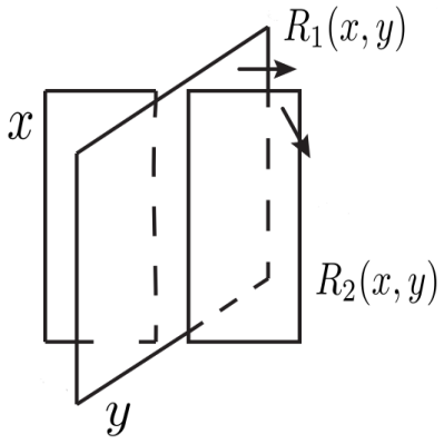
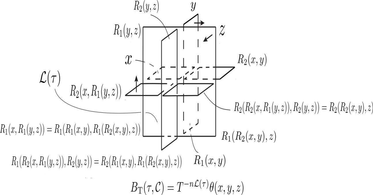
Figure 14. Coloring rule of broken surface diagrams

Figure 15. Assignment of twisted Boltzmann weight to the triple point $\tau$

Analogous to the case of knots, the state sum invariant is defined as follows. Let $K$ be a broken surface diagram and $\mathcal{C}$ be a coloring of $L$ by twisted biquandle $(X,f,R)$. For a triple point $\tau$ in $K$, the source region $R$ and the Alexander numbering $\mathcal{L}(\tau)=\mathcal{L}(R)$ are defined similar to knots (see [4, 8] for more details). Let $\theta\in Z^{3}_{\operatorname{TBQ},(0,n)}(X;M)$ be a cocycle. Then to each triple point $\tau$ with Alexander number $\mathcal{L}(\tau)$, assign a weight $B_{\operatorname{T}}(\tau,\mathcal{C})=T^{-n\mathcal{L}(\tau)}\theta(x,y,z)^{\epsilon(\tau)}$, where $\epsilon(\tau)$ is the sign of the triple point $\tau$ (see [8] for details). An illustration is shown in Figure 15. Now the state sum is defined by

$$\Phi(K)=\sum_{\mathcal{C}}\prod_{\tau}B_{\operatorname{T}}(\tau,\mathcal{C})$$

By checking the invariance of $\Phi(K)$ under the Roseman moves for broken surface diagrams, we obtain the following.

Theorem 7.1.

Let $K_{1}$ and $K_{2}$ are two broken surface diagrams representing the same knotted surface. Then $\Phi(K_{1})=\Phi(K_{2})$.

The proof of the following proposition uses a similar argument as in Proposition 6.2.

Proposition 7.2.

Let $(X,f,R)$ be a twisted biquandle, $M$ a finite $\mathbb{Z}[T,T^{-1}]$-module, and $\phi\in Z^{3}_{\operatorname{TBQ},(0,n)}(X;M)$. If $\phi$ is a coboundary, that is $\phi=\delta^{3}_{(0,n)}(\eta)$, where $\eta\in C^{2}_{\operatorname{TBQ}}(X;M)$, then the state-sum $\Phi(K)$, of a broken surface diagram $K$, is the number of colorings of $K$ by $(X,f,R)$.

8. Concluding remarks

Analogous to Section 6 and Section 7, twisted biquandle cocycles can be used to defined invariants for knot diagrams on compact oriented surfaces up to Reidemeister moves and broken surface diagrams in compact oriented $4$-manifolds up to Roseman moves. Here we briefly describe the process for knots on compact surfaces.

Let $K$ be an oriented knot diagram on a compact oriented surface $S$, and a finite twisted biquandle $(X,f,R)$, where the order of $f$ is $p\in\mathbb{Z}_{\geq 0}$. Let $\phi\in Z^{2}_{\operatorname{TBQ},(0,n)}(X;M)$, where $M$ is a $\mathbb{Z}[T,T^{-1}]$-module and $\mathcal{C}$ a coloring of $K$ by $(X,f,R)$. The diagram $K$ divides $S$ into regions. Fix a base region denoted by $R_{0}$, and define $(\mod p)$-Alexander numbering of the regions (and crossings) as done in Section 6, where $\mathcal{L}(R_{0})=0\mod p$. If $(\mod p)$-Alexander numbering is not defined, then set the state sum invariant $\Phi(K)$ to be $0$. Otherwise, to each crossing $\tau$, assign a twisted Boltzmann weight $B_{\operatorname{T}}(\tau,\mathcal{C})=T^{-n\mathcal{L}(\tau)}(\phi(x,y))^{\epsilon(\tau)}$ as done in Section 6, and define the state-sum

$$\Phi(K)=\sum_{\mathcal{C}}\prod_{\tau}B_{\operatorname{T}}(\tau,\mathcal{C})$$

Note that $\Phi(K)$ depends on the choice of the base region $R_{0}$. To overcome this, we consider $\Phi(K)$ up to action of the free abelian group generated by $T$. Thus we have the following result.

Theorem 8.1.

The state-sum is well defined up to the action of $\mathbb{Z}=<T>$ for knots on surfaces.

8.1. Twisted Yang-Baxter (co)homology theory

In this section, we define a twisted homology theory for Yang-Baxter solutions, which is a generalization of twisted quandle (co)homology theory introduced in [4].

Let $(X,R)$ be a Yang-Baxter solution set, and $m\in\mathbb{Z}$. For each integer $n>0$, let $C_{n}^{\operatorname{YB}}(X)$ be the free $\mathbb{Z}[T,T^{-1}]$-module, and $C_{0}^{\operatorname{YB}}(X)=\{0\}$. We define the $n$-boundary homomorphism

$$\partial_{n}^{(m)}:C_{n}^{\operatorname{YB}}(X)\to C_{n-1}^{\operatorname{YB}}(X)$$

as

$$\partial_{n}^{(m)}=\sum_{i=1}^{n}(-1)\partial_{i,n}^{(m)},$$

where

$$\partial_{i,n}^{(m)}=\partial_{i,n}^{l}-T^{m}\partial_{i,n}^{r}$$

The face maps $\partial_{i,n}^{l}$ and $\partial_{i,n}^{r}$ are illustrated in Figure 2 and Figure 3, respectively. Then $C_{*}^{\operatorname{YB},m}(X)=\{C_{n}^{\operatorname{YB}}(X),\partial_{i,n}^{(m)}\}$ is a chain complex.

As usual, for a given $\mathbb{Z}[T,T^{-1}]$-module $M$, consider the chain and cochain complexes

$$C_{*}^{\operatorname{YB},m}(X;M)=C_{*}^{\operatorname{YB},m}(X)\otimes_{\mathbb{Z}[T,T^{-1}]}M, \partial^{(m)}=\partial^{(m)}\otimes\mathrm{id};$$

$$C^{*}_{\operatorname{YB},m}(X;M)=\operatorname{Hom}_{\mathbb{Z}[T,T^{-1}]}\big{(}C_{*}^{\operatorname{YB},m}(X),M\big{)} \delta_{(m)}=\operatorname{Hom}(\partial^{(m)},\mathrm{id}).$$

The homology and cohomology groups of these complexes are called $m$- Yang-Baxter homology group and cohomology group, and are denoted by $H_{*}^{\operatorname{YB},m}(X;M)$ and $H^{*}_{\operatorname{YB},m}(X;M)$, respectively. We call the (co)cycles in this homology theory $m$-Yang-Baxter $($co$)$cycles.

Let $(X,R)$ be a biquandle. Consider submodule $C_{n}^{\operatorname{D}}(X)$ generated by the elements $(x_{1},\ldots,x_{n})\in X^{n}$, where $R(x_{i},x_{i+1})=(x_{i},x_{i+1})$ for some $1\leq i\leq n-1$. Then we have the following result.

Proposition 8.2.

Let $(X,R)$ be a biquandle. Then $(C_{n}^{\operatorname{D}}(X),\partial_{n}^{(m)})$ is a sub-chain complex of $(C_{n}^{\operatorname{YB}}(X),\partial_{n}^{(m)})$.

Consider the quotient chain complex $C_{*}^{\operatorname{BQ},m}(X)=(C_{n}^{\operatorname{BQ}}(X),\partial_{n}^{(m)})$, where $C_{n}^{\operatorname{BQ}}(X)=C_{n}^{\operatorname{YB}}(X)/\operatorname{C}_{n}^{\operatorname{D}}(X)$. For a $\mathbb{Z}[T,T^{-1}]$-module $M$, define the chain and cochain complexes $C_{*}^{\operatorname{BQ},m}(X;M)=\big{(}C_{n}^{\operatorname{BQ}}(X;M),\partial_{n}^{(m)}\big{)}$ and $C^{*}_{\operatorname{BQ},m}(X;M)=(C^{n}_{\operatorname{BQ}}(X;M),\delta_{(m)}^{n})$, where

$$C_{n}^{\operatorname{BQ}}(X;M) =C_{n}^{\operatorname{BQ}}(X)\otimes_{\mathbb{Z}[T,T^{-1}]}M, \partial_{n}^{(m)}=\partial_{n}^{(m)}\otimes\mathrm{id}_{M},$$

$$C^{n}_{\operatorname{BQ}}(X;M) =\operatorname{Hom}_{\mathbb{Z}[T,T^{-1}]}(C_{n}^{\operatorname{BQ}}(X),M), \delta^{n}_{(m)}=\operatorname{Hom}(\partial_{n}^{(m)},\mathrm{id}_{M})$$

The group of $n$-cocycles are denoted by $Z^{n}_{\operatorname{BQ},m}(X;M)\subseteq C^{n}_{\operatorname{BQ}}(X;M)$. A $2$-cocycle $\phi\in Z^{2}_{\operatorname{BQ},m}(X;M)$ satisfy the following conditions:

• $\phi(x,y)=0$ for all $x,y\in X$ such that $R(x,y)=(x,y)$.

• $$\begin{split}&T^{m}(\phi(R_{1}(x_{1},x_{2}),R_{1}(R_{2}(x_{1},x_{2}),x_{3}))+\\ &\phi(R_{2}(x_{1},x_{2}),x_{3})+T^{m}\big{(}\phi(x_{1},x_{2})\big{)}=\\ &\phi(x_{2},x_{3})+T^{m}\big{(}\phi(x_{1},R_{1}(x_{2},x_{3}))\big{)}+\\ &\phi(R_{2}(x_{1},R_{1}(x_{2},x_{3})),R_{2}(x_{2},x_{3}))\end{split}$$

Now as done in Section 6 and Section 7, for a $2$-cocycle $\phi\in Z^{2}_{\operatorname{BQ},m}(X;M)$, we can use Alexander numbering of a knot (knotted surface) $K$ to use $\phi$ to define state-sum invariant $\Phi(K)$ for $K$.

References

- [1] S. Ashihara. Fundamental biquandles of ribbon 2-knots and ribbon torus-knots with isomorphic fundamental quandles. J. Knot Theory Ramifications, 23(1):1450001, 17, 2014.
- [2] A. Bartholomew and R. Fenn. Quaternionic invariants of virtual knots and links. J. Knot Theory Ramifications, 17(2):231–251, 2008.
- [3] R. J. Baxter. Partition function of the eight-vertex lattice model. Ann. Physics, 70:193–228, 1972.
- [4] J. S. Carter, M. Elhamdadi, and M. Saito. Twisted quandle homology theory and cocycle knot invariants. Algebr. Geom. Topol., 2:95–135, 2002.
- [5] J. S. Carter, M. Elhamdadi, and M. Saito. Homology theory for the set-theoretic Yang-Baxter equation and knot invariants from generalizations of quandles. Fund. Math., 184:31–54, 2004.
- [6] J. S. Carter, D. Jelsovsky, S. Kamada, L. Langford, and M. Saito. Quandle cohomology and state-sum invariants of knotted curves and surfaces. Trans. Amer. Math. Soc., 355(10):3947–3989, 2003.
- [7] J. S. Carter, S. Kamada, and M. Saito. Alexander numbering of knotted surface diagrams. Proc. Amer. Math. Soc., 128(12):3761–3771, 2000.
- [8] J. S. Carter and M. Saito. Knotted surfaces and their diagrams, volume 55 of Mathematical Surveys and Monographs. American Mathematical Society, Providence, RI, 1998.
- [9] J. Ceniceros and S. Nelson. Virtual Yang-Baxter cocycle invariants. Trans. Amer. Math. Soc., 361(10):5263–5283, 2009.
- [10] M. Elhamdadi and M. Singh. Colorings by biquandles and virtual biquandles. arXiv e-prints, page arXiv:2312.05663, Dec. 2023.
- [11] R. Fenn, M. Jordan-Santana, and L. Kauffman. Biquandles and virtual links. Topology Appl., 145(1-3):157–175, 2004.
- [12] V. F. R. Jones. Hecke algebra representations of braid groups and link polynomials. Ann. of Math. (2), 126(2):335–388, 1987.
- [13] V. F. R. Jones. On knot invariants related to some statistical mechanical models. Pacific J. Math., 137(2):311–334, 1989.
- [14] D. Joyce. A classifying invariant of knots, the knot quandle. J. Pure Appl. Algebra, 23(1):37–65, 1982.
- [15] S. Kamada, A. Kawauchi, J. Kim, and S. Y. Lee. Biquandle cohomology and state-sum invariants of links and surface-links. J. Knot Theory Ramifications, 27(11):1843016, 37, 2018.
- [16] L. H. Kauffman. Virtual knot theory. European J. Combin., 20(7):663–690, 1999.
- [17] L. H. Kauffman. Knots and physics, volume 53 of Series on Knots and Everything. World Scientific Publishing Co. Pte. Ltd., Hackensack, NJ, fourth edition, 2013.
- [18] L. H. Kauffman and V. O. Manturov. Virtual biquandles. Fund. Math., 188:103–146, 2005.
- [19] L. H. Kauffman and D. Radford. Bi-oriented quantum algebras, and a generalized Alexander polynomial for virtual links. In Diagrammatic morphisms and applications (San Francisco, CA, 2000), volume 318 of Contemp. Math., pages 113–140. Amer. Math. Soc., Providence, RI, 2003.
- [20] S. V. Matveev. Distributive groupoids in knot theory. Mat. Sb. (N.S.), 119(161)(1):78–88, 160, 1982.
- [21] J. H. Przytycki. Knots and distributive homology: from arc colorings to Yang-Baxter homology. In New ideas in low dimensional topology, volume 56 of Ser. Knots Everything, pages 413–488. World Sci. Publ., Hackensack, NJ, 2015.
- [22] J. H. Przytycki and X. Wang. Equivalence of two definitions of set-theoretic Yang-Baxter homology and general Yang-Baxter homology. J. Knot Theory Ramifications, 27(7):1841013, 15, 2018.
- [23] V. G. Turaev. The Yang-Baxter equation and invariants of links. Invent. Math., 92(3):527–553, 1988.
- [24] C. N. Yang. Some exact results for the many-body problem in one dimension with repulsive delta-function interaction. Phys. Rev. Lett., 19:1312–1315, 1967.