Linear-Quadratic Problems in Systems and Controls
via Covariance Representations and Linear-Conic Duality: Finite-Horizon Case

Abstract

Linear-Quadratic (LQ) problems that arise in systems and controls include the classical optimal control problems of the Linear Quadratic Regulator (LQR) in both its deterministic and stochastic forms, as well as ${\sf H}^{\infty}$-analysis (the Bounded Real Lemma), the Positive Real Lemma, and general Integral Quadratic Constraints (IQCs) tests. We present a unified treatment of all of these problems using an approach which converts linear-quadratic problems to matrix-valued linear-linear problems with a positivity constraint. This is done through a system representation where the joint state/input covariance (the outer product in the deterministic case) matrix is the fundamental object. LQ problems then become infinite-dimensional semidefinite programs, and the key tool used is that of linear-conic duality. Linear Matrix Inequalities (LMIs) emerge naturally as conal constraints on dual problems. Riccati equations characterize extrema of these special LMIs, and therefore provide solutions to the dual problems. The state-feedback structure of all optimal signals in these problems emerge out of alignment (complementary slackness) conditions between primal and dual problems. Perhaps the new insight gained from this approach is that first LMIs, and then second, Riccati equations arise naturally in dual, rather than primal problems. Furthermore, while traditional LQ problems are set up in ${\sf L}^{2}$ spaces of signals, their equivalent covariance-representation problems are most naturally set up in ${\sf L}^{1}$ spaces of matrix-valued signals.

1 Introduction and Motivation

Linear Quadratic (LQ) control problems in systems and controls first arose through the original Linear Quadratic Regulator (LQR) [1], which is an optimal control problem, as well as the celebrated Kalman-Yacubovic-Popov (KYP) Lemma [2, 3, 4]. The KYP Lemma can be considered as a test for an Integral Quadratic Constraint (IQC), which can be phrased as whether an LQ optimal control problem has finite or infinite infima as advocated in the influential paper of Willems [5]. Other IQC tests can be used to characterize robust stability of feedback systems subject to uncertainties that can be characterized by IQCs [6]. Those include the Bounded Real Lemma for testing a system’s ${\sf H}^{\infty}$ (${\sf L}^{2}$-induced) norm, as well as the Positive Real Lemma for testing a system’s passivity. In the same manner as [5], by LQ problems we mean something more general than the LQR problem, namely any problem involving linear dynamics with inputs, and a quadratic form defined jointly on the state and input. The goal is to characterize the extrema of the quadratic form subject to the dynamics as a constraint. The literature on these problems is vast, and will not be summarized here. Notably, Linear Matrix Inequalities (LMIs) and Riccati equations appear frequently as central characters in these intertwined stories.

Connections between LQ problems and LMIs were pointed out by Willems [5]. The books [7, 8] (see also [9]) have since popularized the many uses of LMIs in systems and controls, as well as more general optimization problems. Another theme in [7, 8] is that once a controls problem is formulated as an LMI, then its solution via semidefinite programming is readily achieved. The literature on LMIs is also vast, including a great variety of analysis and synthesis methods, and cannot be summarized here. It is however hard to escape the impression that many arguments with LMIs involve what might be called “algebraic acrobatics”; an LMI for a particular problem is proposed by a skillful acrobat, after which the verification of whether this LMI characterizes the problem at hand is given. One goal of this paper is to step back to try to see a more natural way in which LMIs arise in LQ problems.

It is well known that quadratic programs can be converted to semidefinite programs using Schur complements [8]. Alternatively, for problems with purely quadratic objectives, a reparameterization in terms of the covariance matrix of the variables (tensor product of vectors) renders the objective linear. This idea appears in optimal control problems in [10, 11], where a discrete-time stochastic LQ problem is reformulated such that the joint covariance of the state and control is the new state. The dynamics of covariances are linear but underdetermined, the objective becomes linear, and there are additional positivity constraints on the state expressing that covariance matrices must be non-negative definite. Such a finite-horizon problem then becomes a finite semidefinite program, and it is then shown that the dual problem naturally leads to an LMI. With a similar approach [12, 13, 14] the covariance representation has been used for ${\sf H}^{\infty}$ analysis. More recently [15], a joint “empirical covariance” of the state and control vectors is used as the “state” of a data-driven controller, indicating perhaps that covariance representations are suitable for data-driven control methods as well.

In this paper, a variation of the covariance representation method of [10] is used with a slightly different treatment of the dual problem. Both stochastic and deterministic problems are considered, where the “deterministic covariance” is the rank-one matrix of the outer product of the joint state/input vector. We address continuous-time finite-horizon LQ problems, and view this covariance representation together with its conal constraints as an infinite-dimensional semidefinite program. A natural approach to such problems is to use linear-conic duality and investigate the dual problem. This is where Differential Linear Matrix Inequalities (DLMIs) show up naturally as dual constraints. Since the dual objective is also linear, the dual problem is then solved by extremal solutions (in the Loewner ordering on matrices) of the DLMIs, which in turn are given by Differential Riccati Equations (DREs). We use a Banach space version of weak duality that has a simple proof. Rather than give technical conditions for strong duality, we instead use a complementary slackness (alignment) condition between primal and dual problems. Alignment actually gives additional insight into the solutions, as it shows that all optimal input signals for LQ problems are of the form of static state feedback.

The use of duality in optimal control has some history. In our present context, an LQ problem in covariance representation is most naturally set up in a matrix-valued ${\sf L}^{1}[0,{\scriptstyle T})$ signal space. Other examples of ${\sf L}^{1}$ optimization in control include [16, 17] where duality was used to characterize optimal closed loops as “sparse” impulse responses. Later on [18, 19] finite-dimensional approximations to infinite-dimensional dual problems were used to obtain convergent confidence intervals for numerical solutions to mixed-norm robust control problems in a similar spirit to primal-dual algorithms in semidefinite programming [8, 20].

In a general setting, Vinter [21, Theorem 2.1] developed a duality framework for nonlinear optimal control problems in which the dual constraint is a Partial Differential Inequality (PDI). The number of independent variables in the PDI is one (for time) plus the number of states. In our present context, the dual constraint of an LQ problem is a DLMI, i.e. a ordinary differential inequality. The relation between the PDI of [21] and the DLMI presented here appears similar to that between the HJB equation of dynamic programming (a PDE) whose solutions for LQ problems are quadratic functionals parameterized by solutions to matrix-valued differential Riccati equations. It appears that when restricted to LQ problems, the PDI of [21] collapses to the DLMIs presented here, although those exact connections remain to be explored.

In [22], Rantzer introduced a criterion for stability from almost all initial conditions in terms of a PDI (without time dependence). Density functionals that satisfy this PDI are duals of classic Lyapunov functions. The interpretation of a Lyapunov functions as a cost-to-go in an optimal control problem gives a similar interpretation of a density functional in a dual optimal control problem. More recently [23], duality between this type of analysis and the Koopman representation of dynamical systems have been explored. We again point out that in the present context of LQ problems, DLMIs are parameterized by matrices, which are finite dimensional objects in contrast to the infinite-dimensional objects which solve the PDIs of the more general criteria.

Positive dynamical systems are those whose states have positive components, or more generally evolve in positive cones [24, 25]. For optimal control of positive systems with linear objectives, it is natural to use a dual formulation of the problem as was recently done to provide explicit solutions to the associated HJB equations [26]. For any linear dynamical system, the covariance representation is a linear positive system (in the Loewner order of positive semi-definite matrices), and thus ideas from positive systems appear more generally applicable to not-necessarily-positive systems. A similar theme is used in [27] for analysis of arbitrary linear systems with multiplicative stochastic uncertainty, where an equivalent deterministic system acting on matrix-valued covariance signals is a monotone system.

We finally mention that some of the statements with DLMIs in this paper resemble those in [28] where finite time-horizon IQC problems are investigated, though the techniques we use are somewhat different. In fact, essentially all the results in this paper have appeared elsewhere, and most are a reworking of the ideas of [5] using duality. Thus the novelty is not in the set of ideas presented, but perhaps in the sequencing of these ideas. Whether this is compelling or not is probably a matter of taste. The next subsections summarize the problem formulation and the sequence of steps for using duality to arrive at solutions in terms of DLMIs and DREs. The remainder of the paper is devoted to the details and the necessary background. The paper is written in a tutorial style with an attempt at self containment. Thus many facts that appear in the literature are repeated here for that purpose.

Notation and Terminology

We use the term “positive matrix” to refer to a positive semi-definite matrix, and say “strictly positive” to refer to a positive-definite matrix. The notation $N^{*}$ is used for the transpose of a matrix $N$. Matrices are generally (though not always) denoted by capital letters such as $A$, while operators are generally denoted with calligraphic script, e.g. $\mathcal{L}(X):=AX+XA^{*}$. Capital sans-serif font (such as ${\sf V}$ or ${\sf L}^{1}$), or “blackboard bold” (such as ${\mathbb{R}}$ or $\mathbb{P}$) are used for sets and vector spaces.

1.1 Problem Formulation

Linear-Quadratic Problems (LQPs) in control systems are those where the dynamics are linear, and a cost function is a quadratic form on all the signals in the system

$$\dot{x}{} =~{}Ax+Bv, \begin{array}[]{rcl}x(t_{\rm i})&=&{\rm x}_{\rm i},\\ x(t_{\rm f})&=&{\rm x}_{\rm f},\end{array}$$ (1)

$${\mbox{\large$\mathbf{q}$}}(x,v){} =~{}\int_{t_{\rm i}}^{t_{\rm f}}\begin{bmatrix}x\\ v\end{bmatrix}^{*}{\begin{bmatrix}&&\\ &{\bm{Q}}&\\ &&\end{bmatrix}}\begin{bmatrix}x\\ v\end{bmatrix}dt~{}=:~{}\int_{t_{\rm i}}^{t_{\rm f}}{\sf q}(x,v)~{}dt,$$

where either initial ${\rm x}_{\rm i}$ or final ${\rm x}_{\rm f}$ state maybe specified or free, and initial and final times $t_{\rm i}$ and $t_{\rm f}$ may be finite or infinite. ${\bm{Q}}$ is a matrix that determines the quadratic form ${\mbox{\large$\mathbf{q}$}}(x,v)$. This is a powerful general framework which encompasses many different problems.

• The signal $v$ can play different roles. In the LQR problem it is a control, and the problem is to determine the optimal control that minimizes $\mathbf{q}$. In other problems such as ${\sf H}^{\infty}$ analysis or more generally Integral Quadratic Constraints (IQCs), $v$ is an exogenous signal and the analysis problem is to determine whether $\mathbf{q}$ remains positive or finite for all possible such exogenous signals.

• Without loss of generality, the matrix ${\bm{Q}}$ is taken as symmetric. It may be positive or have mixed signature depending on the problem at hand.

• The time horizon $t_{\rm f}-t_{\rm i}$ can be finite or infinite. Usually for finite horizons, there are no conceptual differences between the cases of time-invariant or time-varying systems. For infinite horizon problems issues of stability arise that need to be characterized.

The diversity of the problems that can be formulated as (1) is best appreciated by listing some of the well-known ones. The following is a non-comprehensive list by way of examples.

• The Linear Quadratic Regulator (LQR): In this problem the input signal $v$ is a control, traditionally denoted by $u$. Given an initial state ${\rm x}_{\rm i}$, it is desired to drive (“regulate”) this state to zero while minimizing an objective that is a combination of regulation and control costs

  $${\sf q}(x,u)~{}:=~{}x^{*}Qx+2x^{*}Nu+u^{*}Ru~{}=~{}\begin{bmatrix}x\\ u\end{bmatrix}^{*}\begin{bmatrix}Q&N\\ N^{*}&R\end{bmatrix}\begin{bmatrix}x\\ u\end{bmatrix}~{}=:~{}\begin{bmatrix}x\\ u\end{bmatrix}^{*}{\begin{bmatrix}&&\\ &{\bm{Q}}&\\ &&\end{bmatrix}}\begin{bmatrix}x\\ u\end{bmatrix}$$

  In this problem $x(t_{\rm i})={\rm x}_{\rm i}$ is given and $x(t_{\rm f})$ is free. The “disturbance” in this setting is the non-zero initial state, and the task of the control $u$ is to ameliorate the effect of this initial disturbance by regulating the state back to zero (equilibrium). In this setting, $x$ is uniquely determined by $u$, and the task is to find $u$ that minimizes this objective

  $$\inf_{u}{\mbox{\large$\mathbf{q}$}}(x,u),\hskip 20.00003pt\mbox{subject to}\hskip 20.00003pt\dot{x}=Ax+Bu,\hskip 10.00002ptx(t_{\rm i})={\rm x}_{\rm i}.$$

  In this problem, we assume $Q\geq 0$, $R>0$, and $N$ is chosen subject to the constraint ${\bm{Q}}\geq 0$ (not to be confused with its submatrix $Q$).

• Kalman-Yacubovic-Popov (KYP) Lemma and Integral Quadratic Constraints (IQCs): The KYP Lemma is fundamentally about whether a quadratic form like (1) is nonnegative (or alternatively, nonpositive) for all signals consistent with the system dynamics. It is usually stated for infinite time-horizon problems, and has frequency-domain as well as a time-domain characterizations. More modern uses of the lemma use the formalism of IQCs for various robustness analysis problems. The two most commonly used instances of the KYP lemma are the “positive real”, and the “bounded real” lemmas.

  • Characterizing Passivity: (aka The Positive-Real Lemma) This is an analysis problem, so the input is viewed as an exogenous signal in ${\sf L}^{2}[t_{\rm i},t_{\rm f}]$. A system is called passive from $v$ to an output $z=Cx+Dv$ if the inner product between the input and output is positive. In this case

    $${\sf q}(x,v)~{}:=~{}z^{*}v=(Cx+Dv)^{*}v=x^{*}C^{*}v+v^{*}D^{*}v=\frac{1}{2}\begin{bmatrix}x\\ v\end{bmatrix}^{*}\begin{bmatrix}0&C^{*}\\ C&D\text{+}D^{*}\end{bmatrix}\begin{bmatrix}x\\ v\end{bmatrix},$$ (2)

    and initial conditions are zero $x(0)=0$. In this problem we want to check whether this quadratic form is positive for all signals $(x,v)$ consistent with the system’s equations

    $$\forall w,~{}\scaleobj{.8}{\int_{{t_{\rm i}}}^{{t_{\rm f}}}}{\sf q}(x,v)~{}dt~{}\geq~{}0\hskip 20.00003pt\Leftrightarrow\hskip 20.00003pt\inf_{w}\scaleobj{.8}{\int_{{t_{\rm i}}}^{{t_{\rm f}}}}{\sf q}(x,v)~{}dt~{}=~{}0.$$

  • Characterizing ${\sf L}^{2}$-induced (${{\sf H}^{\infty}}$) Norms: (aka The Bounded-Real Lemma): This is another analysis problem with zero initial state $x(0)=0$. The system has ${\sf L}^{2}(0,{\scriptstyle T})$-induced norm less than a given number $\gamma$ from $v$ to an output $z=Cx$ iff $\int_{0}^{{\scriptscriptstyle T}}{\sf q}(x,v)dt\geq 0$, where

    $${\sf q}(x,w)~{}:=~{}\gamma^{2}v^{*}v-z^{*}z~{}=~{}\gamma^{2}v^{*}v-x^{*}C^{*}Cx~{}=~{}\begin{bmatrix}x\\ v\end{bmatrix}^{*}\begin{bmatrix}\text{-}C^{*}C&0\\ 0&\gamma^{2}I\end{bmatrix}\begin{bmatrix}x\\ v\end{bmatrix},$$ (3)

    for all inputs $v$. Again, this is a problem of characterizing whether a quadratic form defined on the system’s signals is always positive, which as in the passivity problem, is the same as insuring that the infimum over all $v$ is zero.

    Note that an equivalent formulation would also be

    $${\sf q}(x,v)~{}:=~{}x^{*}C^{*}Cx-\gamma^{2}v^{*}v~{}=~{}\begin{bmatrix}x\\ v\end{bmatrix}^{{*}}\begin{bmatrix}C^{*}C&0\\ 0&\text{-}\gamma^{2}I\end{bmatrix}\begin{bmatrix}x\\ v\end{bmatrix},$$

    with the condition that $\int_{0}^{{\scriptscriptstyle T}}{\sf q}(x,v)dt\leq 0$, i.e. checking that the supremum of this quadratic form is zero. This alternative, but equivalent, formulation is sometimes encountered in the literature. We adopt here the formulation (3) instead since we want to treat all problems as infimization problems so that a single result can be stated for all LQP problems in a manner similar to the LQR problem.

Derivations of the statements above regarding the ${{\sf H}^{\infty}}$ norm and passivity are included in Appendix A.2 for reference. As already stated, we adopt a unifying convention for all problems whereby $R>0$ with no restriction on the remaining matrices.

1.2 Outline of the Present Approach

As an overview, we now summarize the main steps of the present approach, with details to be presented in later sections. The key idea is to recast the linear-quadratic problem (1) as a linear-linear problem for matrix-valued signals, but with an additional positivity constraint as follows. Restating (1)

$$\dot{x}~{} =~{}Ax+Bv,\hskip 20.00003ptx(0)={\rm x}_{\rm i},$$ (4)

$${\mbox{\large$\mathbf{q}$}}(x,w)~{} =~{}\int_{0}^{{\scriptscriptstyle T}}\begin{bmatrix}x\\ v\end{bmatrix}^{*}{\begin{bmatrix}&&\\ &{\bm{Q}}&\\ &&\end{bmatrix}}\begin{bmatrix}x\\ v\end{bmatrix}dt~{}=:~{}\int_{0}^{{\scriptscriptstyle T}}{\sf q}(x,v)~{}dt,$$ (5)

observe that if we define the following matrix-valued signal, which is the outer (tensor) product of the original problem variables

$$\Sigma(t)~{}:=~{}\begin{bmatrix}x(t)\\ v(t)\end{bmatrix}\begin{bmatrix}x^{*}(t)&v^{*}(t)\end{bmatrix}~{}=:~{}\begin{bmatrix}\Sigma_{xx}(t)&\Sigma_{xv}(t)\\ \Sigma_{xv}^{*}(t)&\Sigma_{vv}(t)\end{bmatrix},\hskip 20.00003pt$$ (6)

then the quadratic objective $\mathbf{q}$ becomes linear in $\Sigma$

$${\mbox{\large$\mathbf{q}$}}~{}:=\!\!\int_{0}^{{\scriptscriptstyle T}}\!\!{\begin{bmatrix}x^{*}&v^{*}\end{bmatrix}{\begin{bmatrix}&&\\ &{\bm{Q}}&\\ &&\end{bmatrix}}\begin{bmatrix}x\\ v\end{bmatrix}}dt=\int_{0}^{{\scriptscriptstyle T}}\!\!{\rm tr}\!\left({\begin{bmatrix}&&\\ &{\bm{Q}}&\\ &&\end{bmatrix}}{\begin{bmatrix}x\\ v\end{bmatrix}\begin{bmatrix}x^{*}&v^{*}\end{bmatrix}}\right)dt=:\int_{0}^{{\scriptscriptstyle T}}\left<{\bm{Q}}\bm{,}\Sigma\rule{0.0pt}{9.10004pt}\right>~{}dt,$$ (7)

where $\left<{\bm{Q}}\bm{,}\Sigma\right>:={\rm tr}\!\left({\bm{Q}}^{*}\Sigma\right)$ is the inner product on matrices. If $v$ is stochastic, then we would take expectations in (6), and $\Sigma$ would then be the joint input-state covariance matrix. If $v$ is deterministic, then $\Sigma$ can still be thought of as a “deterministic covariance”, or as already stated, the outer (tensor) product of the vector signal $(x,v)$ with itself. In this case, $\Sigma$ has the additional property of always being a rank-one matrix.

A differential equation for the $\Sigma_{xx}$ portion of $\Sigma$ can be derived from the system dynamics (4) as follows

$$\frac{d}{dt}xx^{*}~{} =~{}\dot{x}x^{*}+x\dot{x}^{*}~{}=~{}(Ax+Bv)~{}x^{*}+x~{}(Ax+Bv)^{*}$$

$$=~{}A~{}xx^{*}+B~{}vx^{*}+xx^{*}~{}A^{*}+xv^{*}~{}B^{*}$$

$$\Leftrightarrow~{}~{}\dot{\Sigma}_{xx} =\begin{bmatrix}A&B\end{bmatrix}\begin{bmatrix}\Sigma_{xx}\\ \Sigma_{xv}^{*}\end{bmatrix}+\begin{bmatrix}\Sigma_{xx}&\Sigma_{xv}\end{bmatrix}\begin{bmatrix}A^{*}\\ B^{*}\end{bmatrix} \Sigma_{xx}(0) ={\rm x}_{\rm i}{\rm x}_{\rm i}^{*}$$

$$\Leftrightarrow~{}~{}\begin{bmatrix}I&0\end{bmatrix}{\begin{bmatrix}&&\\ &{\color[rgb]{0,0.3,0.7}\dot{\Sigma}}&\\ &&\end{bmatrix}}\begin{bmatrix}I\\ 0\end{bmatrix} =\begin{bmatrix}A&B\end{bmatrix}{\begin{bmatrix}&&\\ &{\color[rgb]{0,0.3,0.7}\Sigma}&\\ &&\end{bmatrix}}\begin{bmatrix}I\\ 0\end{bmatrix}+\begin{bmatrix}I&0\end{bmatrix}{\begin{bmatrix}&&\\ &{\color[rgb]{0,0.3,0.7}\Sigma}&\\ &&\end{bmatrix}}\begin{bmatrix}A^{*}\\ B^{*}\end{bmatrix}, \begin{bmatrix}I&0\end{bmatrix}{\begin{bmatrix}&&\\ &\!\!{\color[rgb]{0,0.3,0.7}\Sigma(0)}\!\!\!\!&\\ &&\end{bmatrix}}\begin{bmatrix}I\\ 0\end{bmatrix} ={\rm x}_{\rm i}{\rm x}_{\rm i}^{*},$$ (8)

where matrix dimensions are shown for emphasis. This is a linear, but somewhat unusual differential equation. Only a subset of the components of the derivative $\dot{\Sigma}(t)$ are given as a linear function of $\Sigma(t)$. Thus this is a highly under-deteremined system of differential equations, and has non-unique solutions even if full initial or final conditions are specified.

To appreciate the structure of (8) more precisely, define the linear, matrix-valued operators on matrices

$${\mathcal{E}}\big{(}\Sigma\big{)}:=\begin{bmatrix}I&0\end{bmatrix}{\begin{bmatrix}&&\\ &\Sigma&\\ &&\end{bmatrix}}\begin{bmatrix}I\\ 0\end{bmatrix},\hskip 20.00003pt\mathcal{A}\big{(}\Sigma\big{)}:=\begin{bmatrix}A&B\end{bmatrix}{\begin{bmatrix}&&\\ &\Sigma&\\ &&\end{bmatrix}}\begin{bmatrix}I\\ 0\end{bmatrix}+\begin{bmatrix}I&0\end{bmatrix}{\begin{bmatrix}&&\\ &\Sigma&\\ &&\end{bmatrix}}\begin{bmatrix}A^{*}\\ B^{*}\end{bmatrix},$$ (9)

and the differential equation (8) can now be written as

$${\mathcal{E}}\big{(}\dot{\Sigma}(t)\big{)}~{}=~{}\mathcal{A}\big{(}\Sigma(t)\big{)},\hskip 20.00003pt\hskip 20.00003pt{\mathcal{E}}\big{(}\Sigma(0)\big{)}={\rm x}_{\rm i}{\rm x}_{\rm i}^{*}=:{\sf X}_{\rm i}.$$ (10)

Note that the operator ${\mathcal{E}}$ is not invertible, it takes $(n+m)\times(n+m)$ matrices (where $n:=\dim(x)$ and $m:=\dim(v)$) to $n\times n$ matrices. The differential equation above thus belongs to the class of “descriptor systems”, and non-uniqueness of solutions is typical for some classes of descriptor systems. It is important to understand the relation between the original vector differential equation (4) and the matrix differential equation (8). In the deterministic case, any solution of the vector differential equation gives a solution of the matrix differential equation by taking the outer product of the solution vector $(x,v)$ with itself. However, to go from solutions of the matrix to the original vector equation, one must impose a rank-one constraint on $\Sigma$ as follows

$${\mathcal{E}}\big{(}\dot{\Sigma}\big{)} =\mathcal{A}\big{(}\Sigma\big{)}, t\in[0,{\scriptstyle T}],$$ (11)

$$\hskip 20.00003pt\Sigma \geq 0,~{}{\rm\bf rk}\!\left(\Sigma\right)=1,~{}{\mathcal{E}}\big{(}\Sigma(0)\big{)}={\rm x}_{\rm i}{\rm x}_{\rm i}^{*},$$

where ${\rm\bf rk}\!\left(\Sigma\right):={\rm rank}(\Sigma)$. Given any solution of (11) we can factor the rank-one positive matrix $\Sigma(t)=z(t)z^{*}(t)$, and then partition the vector $z$ conformably with the partitions of ${\mathcal{E}}$ and $\mathcal{A}$ and obtain $z(t)=:\begin{bmatrix}x(t)\\ v(t)\end{bmatrix}$ which solve the original differential equation (4). Thus there is a one-to-one correspondence between solutions of (4) and solutions of (11).

Now the original LQ problem and the equivalent covariance problem can be stated as follows

$$\inf_{\begin{array}[]{rcl}\scriptstyle\dot{x}&\scriptstyle=&\scriptstyle Ax+Bv\\ \scriptstyle{\rm x}_{\rm i}&\scriptstyle=&\scriptstyle x(0)\end{array}}\scaleobj{.8}{\int_{{0}}^{{{\scriptscriptstyle T}}}}{\sf q}(x,v)dt\hskip 20.00003pt=\inf_{\begin{array}[]{rcl}\scriptstyle{\mathcal{E}}(\dot{\Sigma})&\scriptstyle=&\scriptstyle\mathcal{A}(\Sigma),\\ \scriptstyle{\mathcal{E}}(\Sigma(0))&\scriptstyle=&\scriptstyle{\sf X}_{\rm i},~{}\scriptstyle{\rm\bf rk}\left(\Sigma\right)\scriptstyle=\scriptstyle 1,~{}\Sigma\geq 0\end{array}}\scaleobj{.8}{\int_{{0}}^{{{\scriptscriptstyle T}}}}\left<{\bm{Q}}\bm{,}\Sigma\right>dt$$ (12)

The covariance problem now has linear dynamics, and a linear objective. We have however two additional constraints, a positivity (cone) constraint $\Sigma\geq 0$, and a rank constraint. The latter makes the problem non-convex even if the original linear-quadratic problem is convex. This turns out to be a red-herring. As explained later in (35), since the objective is a linear functional, the non-convex rank-one cone of matrices can be replaced by its convex hull, the cone of all positive matrices. In addition, rank-one solutions always exists even if the infimum is taken over the entire cone of positive matrices.

The important new ingredient in (12) is the positivity, or cone constraint $\Sigma\geq 0$. Optimization problems with linear constraints and objectives together with a cone constraint belong to the class of linear-conic optimization problems. The main tool for the study of such problems is linear-conic duality (summarized in Section 2.4). For the current example, we preview the result stated in Theorem 12, and how it can be used to address all LQ Problems in four main steps.

1. The differential equation (10) for $\Sigma$ can be converted to a linear constraint in function space by integrating it forward in time

   $$\left.\begin{array}[]{rcl}{\mathcal{E}}\big{(}\dot{\Sigma}\big{)}&=&\mathcal{A}\big{(}\Sigma\big{)}\\ {\mathcal{E}}(\Sigma(0))&=&{\sf X}_{\rm i}\end{array}\right\}\hskip 20.00003pt\Leftrightarrow\hskip 20.00003pt\left({\mathcal{E}}-{\sf{\bm{I}}}_{\sf f}\mathcal{A}\right)(\Sigma)~{}=~{}\mathfrak{h}{\sf X}_{\rm i},$$ (13)

   where ${\sf{\bm{I}}}_{\sf f}$ is the forward integration operator, and $\mathfrak{h}$ is the unit-step (Heaviside) function (thus $\mathfrak{h}{\sf X}_{\rm i}$ is a constant, matrix-valued function with value ${\sf X}_{\rm i}$). $\left({\mathcal{E}}-{\sf{\bm{I}}}_{\sf f}\mathcal{A}\right)$ is a bounded operator on (matrix-valued) ${\sf L}^{1}[0,{\scriptstyle T}]$, and equation (13) is a linear equality constraint on $\Sigma$.

2. The “weak duality” statement for the covariance problem (12) is

   $${\begin{array}[]{rcl}\displaystyle\inf_{\Sigma\in{\sf L}^{1}(0,{\scriptscriptstyle T})}&&\displaystyle\scaleobj{.8}{\int_{{0}}^{{{\scriptscriptstyle T}}}}\left<{\bm{Q}}\bm{,}\Sigma\right>~{}dt\\ \big{(}{\mathcal{E}}-{\sf{\bm{I}}}_{\sf f}\mathcal{A}\big{)}(\Sigma)&=&\mathfrak{h}{\sf X}_{\rm i}\rule{0.0pt}{15.00002pt}\\ {\rm\bf rk}\left(\Sigma\right)&=&1,~{}\Sigma\geq 0\end{array}}\hskip 20.00003pt\hskip 20.00003pt\geq\hskip 20.00003pt{\begin{array}[]{rcl}\displaystyle\sup_{Y\in{\sf L}^{\infty}(0,{\scriptscriptstyle T})}&&\displaystyle\scaleobj{.8}{\int_{{0}}^{{T}}}\left<Y\bm{,}{\sf X}_{\rm i}\right>~{}dt\\ {\bm{Q}}-\big{(}{\mathcal{E}}-{\sf{\bm{I}}}_{\sf f}\mathcal{A}\big{)}^{{\bm{*}}}(Y)&\geq&0\rule{0.0pt}{15.00002pt}\end{array}}$$ (14)

   where the dual variable $Y$ is a matrix-valued function over $[0,{\scriptstyle T}]$. Note that since $(x,v)$ are in ${\sf L}^{2}(0,{\scriptstyle T})$, then their outer product $\Sigma\in{\sf L}^{1}_{{\mathbb{S}}_{n}}(0,{\scriptstyle T})$, the ${\sf L}^{1}$ space of functions taking values in ${\mathbb{S}}_{n}$, the space of $n\times n$ symmetric matrices.

   The key to the dual problem is the dual inequality constraint ${\bm{Q}}-\big{(}{\mathcal{E}}-{\sf{\bm{I}}}_{\sf f}\mathcal{A}\big{)}^{{\bm{*}}}(Y)\geq 0$, whose structure depends on the adjoint operator $\big{(}{\mathcal{E}}-{\sf{\bm{I}}}_{\sf f}\mathcal{A}\big{)}^{{\bm{*}}}$. A simple adjoint calculation (Section 2.2) shows that

   $$\big{(}{\mathcal{E}}-{\sf{\bm{I}}}_{\sf f}\mathcal{A}\big{)}^{{\bm{*}}}(Y)~{}=~{}{\mathcal{E}}^{{\bm{*}}}(Y)-\mathcal{A}^{{\bm{*}}}({\sf{\bm{I}}}_{\sf\bm{b}}Y)~{} =~{}\begin{bmatrix}I\\ 0\end{bmatrix}Y\begin{bmatrix}I&0\end{bmatrix}-\begin{bmatrix}A^{*}\\ B^{*}\end{bmatrix}\big{(}{\sf{\bm{I}}}_{\sf\bm{b}}Y\big{)}\begin{bmatrix}I&0\end{bmatrix}-\begin{bmatrix}I\\ 0\end{bmatrix}\big{(}{\sf{\bm{I}}}_{\sf\bm{b}}Y\big{)}\begin{bmatrix}A&B\end{bmatrix}$$

   $$\Rightarrow\hskip 20.00003pt{\bm{Q}}-({\mathcal{E}}-{\sf{\bm{I}}}_{\sf f}\mathcal{A})^{*}(Y)~{} =~{}{\bm{Q}}-\left({\mathcal{E}}\left({\dot{\Lambda}}\right)-\mathcal{A}^{*}(\Lambda)\right)~{}=~{}{\bm{Q}}+\begin{bmatrix}{\dot{\Lambda}}+A^{*}\Lambda+\Lambda A&\Lambda B\\ B^{*}\Lambda&0\end{bmatrix},$$

   where the dual variable $Y$ is replaced with $\Lambda:={\sf{\bm{I}}}_{\sf\bm{b}}Y$, the backwards integral of $Y$ (which implies $Y=-{\dot{\Lambda}}$).

   Thus a Differential Linear Matrix Inequality (DLMI) arises out of the dual cone constraint $\big{(}{\mathcal{E}}-{\sf{\bm{I}}}_{\sf f}\mathcal{A}\big{)}^{{\bm{*}}}(Y)\geq 0$ when expressed in terms of the backwards integral of $Y$. Note how the structure of the DLMI is really a corollary of the structure of the operators ${\mathcal{E}}$, $\mathcal{A}$, and their adjoints!

   Conic duality thus shows that LMIs arise naturally from problems dual to covariance optimization problems. A similar statement is much less transparent if one only considers the original problem statement (4) without a covariance reformulation.

3. Differential Riccati equations give extremal solutions to DLMIs, which are then shown to be the solutions to the dual problem since the objective is a linear functional in the dual variables $Y$ or $\Lambda$. Thus, Riccati equations also arise naturally from conic duality. However, In this framework the DLMIs come first, and Riccati equations arise second as extremal solutions to the DLMIs. Riccati equations can be thought of in this context as a technique to solve these special DLMIs (and LMIs) rather than using general-purpose convex optimization methods.

4. The duality gap will be shown to be zero by constructing optimal primal and dual solutions together with an alignment (complementary slackness) condition between them. Specifically, linear-conic duality states that if there exists primal and dual variables ${\bar{\Sigma}}$ and ${\bar{\Lambda}}$ such that

   $$0~{}=~{}\left<{\bm{Q}}-{\mathcal{E}}^{*}(\dot{{\bar{\Lambda}}})-\mathcal{A}^{*}({\bar{\Lambda}})\bm{,}{\bar{\Sigma}}\right>,$$ (15)

   then ${\bar{\Sigma}}$ and ${\bar{\Lambda}}$ are optimal for the primal and dual respectively, and the duality gap is zero. The optimal solution ${\bar{\Lambda}}$ to the dual problem is the solution of a Riccati equation. A classic argument implies that this solution gives a minimal-rank factorization of the LMI matrix as follows

   $${\bm{Q}}-{\mathcal{E}}^{*}(\dot{{\bar{\Lambda}}})-\mathcal{A}^{*}({\bar{\Lambda}})={\bm{Q}}+\begin{bmatrix}\dot{{\bar{\Lambda}}}+A^{*}{\bar{\Lambda}}+{\bar{\Lambda}}A&{\bar{\Lambda}}B\\ B^{*}{\bar{\Lambda}}&0\end{bmatrix}=\begin{bmatrix}{\bar{\Lambda}}BR^{\text{-}\frac{1}{2}}\\ R^{\frac{1}{2}}\end{bmatrix}\begin{bmatrix}R^{\text{-}\frac{1}{2}}B^{*}{\bar{\Lambda}}B&R^{\frac{1}{2}}\end{bmatrix}.$$

   Since any possible ${\bar{\Sigma}}$ must be of the form (6), the alignment condition (15) then reads

   $$0=\left<\begin{bmatrix}{\bar{\Lambda}}BR^{\text{-}\frac{1}{2}}\\ R^{\frac{1}{2}}\end{bmatrix}\begin{bmatrix}R^{\text{-}\frac{1}{2}}B^{*}{\bar{\Lambda}}&R^{\frac{1}{2}}\end{bmatrix}\bm{,}\begin{bmatrix}{\bar{x}}\\ {\bar{v}}\end{bmatrix}\begin{bmatrix}{\bar{x}}^{*}&{\bar{v}}^{*}\end{bmatrix}\right>\hskip 20.00003pt \Rightarrow\hskip 20.00003pt\begin{bmatrix}R^{\text{-}\frac{1}{2}}B^{*}{\bar{\Lambda}}&R^{\frac{1}{2}}\end{bmatrix}\begin{bmatrix}{\bar{x}}\\ {\bar{v}}\end{bmatrix}=0$$

   $$\Rightarrow\hskip 20.00003pt{\bar{v}}~{}=~{}\left(R^{\text{-}1}B^{*}{\bar{\Lambda}}\right){\bar{x}},$$

   where the first implication is a property of symmetric factorizations of any two positive matrices (Lemma 3).

   Thus the state-feedback nature of optimal solutions of any LQ problem is a consequence of the alignment condition (15) between primal and dual solutions.

This note deals primarily with finite-horizon cases of LQ problems. The infinite-horizon case will be reported in Part II. The exposition in this note is meant to be tutorial and self contained. The organization is as follows. Section 2 collects the necessary mathematical preliminaries needed to use linear-conic duality in a function (Banach) space, as well as some facts about cones of matrices and their duals. In Section 3 we investigate Differential Linear Matrix Inequalities (DLMIs) and show that Differential Riccati Equations (DREs) derived from them give maximal and minimal solutions to the DLMIs. With all the preliminaries established, Section 4 gives the solution to the classic Linear Quadratic Regulator (LQR) problem. Section 5 treats the stochastic version of the LQR problem and illustrates the covariance approach for stochastic problems. Section 6 treats the general Integral Quadratic Constraints (IQCs) case, and we work out the various special IQC-type problems such as the Bounded Real Lemma and the Positive Real Lemma in their finite-horizon versions. Some arguments are relegated to appendices in order not to disrupt the exposition of the key ideas.

2 Mathematical Preliminaries

In this section we collect some mathematical preliminaries that will be needed. The presentation is meant to be self contained and tutorial.

2.1 Matrix Signals and their Norms

We will be concerned with the vector space ${\mathbb{R}}^{n\times n}$ of $n\times n$ matrices, and in particular its subspace ${\mathbb{S}}_{n}\subset{\mathbb{R}}^{n\times n}$ of symmetric matrices. The vector space ${\mathbb{R}}^{n\times n}$ has a natural inner product given by

$$\left<H\bm{,}M\right>~{}:=~{}{\rm tr}\!\left(H^{*}M\right).$$ (16)

This is simply the total sum of the element-by-element product of two matrices $H$ and $M$. Equivalently, if each matrix $H$ and $M$ is expanded as a single vector by stacking its columns over each other, the above sum would simply be the dot product of the two vectors. We note that this inner product generates the Frobenius norm $\|M\|_{F}^{2}={\rm tr}\!\left(M^{*}M\right)=\left<M\bm{,}M\right>$ on matrices.

If we restrict attention to the subspace ${\mathbb{S}}_{n}\subset{\mathbb{R}}^{n\times n}$ of $n\times n$ symmetric matrices, the algebraic dual of ${\mathbb{S}}_{n}$ is itself since the action of any matrix $H$ on a symmetric matrix $M$ is

$$\left<H\bm{,}M\right>~{}=~{}{\rm tr}\!\left(H^{*}M\right)~{}=~{}\left({\rm tr}\!\left(H^{*}M\right)+{\rm tr}\!\left(MH\right)\rule{0.0pt}{9.10004pt}\right)/2~{}=~{}\left({\rm tr}\!\left(H^{*}M\right)+{\rm tr}\!\left(HM\right)\rule{0.0pt}{9.10004pt}\right)/2~{}=~{}{\rm tr}\!\left({\scriptstyle\frac{1}{2}}(H^{*}+H)~{}M\right),$$

and therefore the action of $\left<H\bm{,}.\right>$ on ${\mathbb{S}}_{n}$ is the same as the action of its symmetrization $\left<(H^{*}+H)/2\bm{,}.\right>$.

We will need norms other than the Frobenius norm on matrices, and therefore a different interpretation of (16) as a linear functional action (of $H$ on $M$). When $M$ is a symmetric positive matrix (like $\Sigma$ in (6)), its trace is the quantity of interest. The trace on positive matrices is a special case of the “nuclear norm” on $n\times n$ matrices defined as

$$\|M\|_{1}~{}:=~{}\sum_{i=1}^{n}\sigma_{i}(M),$$ (17)

where $\left\{\sigma_{i}(M)\right\}$ are the singular values of $M$. When $M$ is symmetric and positive, ${\rm tr}\!\left(M\right)=\|M\|_{1}$, but the definition (17) applies to any matrix. We denote the space of symmetric $n\times n$ matrices with the $\|.\|_{1}$ norm by $\left({\mathbb{S}}_{n},\|.\|_{1}\right)$. The norm dual to $\|.\|_{1}$ is the maximum singular value norm

$$\|H\|_{\infty}~{}:=~{}\max_{1\leq i\leq n}\sigma_{i}(H).$$

The fact that this norm is dual to $\|.\|_{1}$ follows from the following tight “trace duality” inequality whose proof is given in Appendix A.1

$$\left<H\bm{,}M\right>~{}:=~{}{\rm tr}\!\left(HM\right)~{}\leq~{}\|H\|_{\infty}\|M\|_{1},\hskip 20.00003pt\hskip 20.00003pt\sup_{\|M\|_{1}\leq 1}{\rm tr}\!\left(HM\right)=\|H\|_{\infty}.$$

Thus the space dual to $\left({\mathbb{S}}_{n},\|.\|_{1}\right)$ is $\left({\mathbb{S}}_{n},\|.\|_{\infty}\right)$. More generally, we can define the space $\left({\mathbb{S}}_{n},\|.\|_{p}\right)$ for $p\in(1,\infty)$ with the norm

$$\|M\|_{p}^{p}~{}:=~{}\sum_{i=1}^{n}\left(\sigma_{i}(M)\right)^{p},$$

and the space dual to it is $\left({\mathbb{S}}_{n},\|.\|_{q}\right)$ with $1/p+1/q=1$. However, this level of generality is not needed here.

We will also need to consider norms and linear functional actions on matrix-valued functions of time. To motivate the definition we will shortly introduce, consider again the covariance matrix (6) and observe that

$$\int_{0}^{T}{\rm tr}\!\left(\Sigma(t)\rule{0.0pt}{10.00002pt}\right)~{}dt~{}=~{}\int_{0}^{T}{\rm tr}\!\left(\begin{bmatrix}x(t)\\ v(t)\end{bmatrix}\begin{bmatrix}x^{*}(t)&v^{*}(t)\end{bmatrix}\right)~{}dt~{}=~{}\int_{0}^{T}\left(x^{*}(t)x(t)+v^{*}(t)v(t)\rule{0.0pt}{10.00002pt}\right)~{}dt,$$

where ${\scriptstyle T}=\infty$ is a possible limit of this integral. If all signals $(v,x)$ need to have finite ${{\sf L}}^{\!2}$ norms, then we should require $\Sigma$ itself to have finite trace norm integrated over the time interval. We therefore require our matrix-valued signals to be in the following Banach space

$${{\sf L}}^{\!1}_{{\mathbb{S}}_{n}}(0,{\scriptstyle T})~{}:=~{}\left\{M:(0,{\scriptstyle T})\rightarrow{\mathbb{S}}_{n};~{}\|M\|_{1}:=\scaleobj{.8}{\int_{{0}}^{{T}}}\|M(t)\|_{1}~{}dt~{}<\infty\right\},\hskip 20.00003pt{\scriptstyle T}<\infty,~{}\mbox{or}~{}{\scriptstyle T}=\infty.$$ (18)

Note that the matrix norm $\|M(t)\|_{1}$ is the one defined in (17), and we use the same notation $\|.\|_{1}$ to denote a matrix norm as well as the above norm on matrix-valued functions.

The space dual to (18) is the following ${{\sf L}}^{\!\!\infty}$ space

$${{\sf L}}^{\!\!\infty}_{{\mathbb{S}}_{n}}(0,{\scriptstyle T}):=\left\{H:(0,{\scriptstyle T})\rightarrow{\mathbb{S}}_{n};~{}\|H\|_{\infty}:=\sup_{t\in(0,{\scriptstyle T})}\left(\sigma_{\max}\left(H(t)\rule{0.0pt}{9.10004pt}\right)\rule{0.0pt}{10.00002pt}\right)~{}<\infty\right\},\hskip 20.00003pt{\scriptstyle T}<\infty,~{}\mbox{or}~{}{\scriptstyle T}=\infty.$$ (19)

The linear functional action is defined as follows

$$\left<H\bm{,}M\right>~{}:=~{}\scaleobj{.8}{\int_{{0}}^{{T}}}\left<H(t)\bm{,}M(t)\right>~{}dt~{}:=~{}\scaleobj{.8}{\int_{{0}}^{{T}}}{\rm tr}\!\left(\rule{0.0pt}{10.00002pt}H(t)~{}M(t)\right)~{}dt,\hskip 20.00003ptM\in{{\sf L}}^{\!1}(0,{\scriptstyle T}),\hskip 20.00003ptH\in{{\sf L}}^{\!\!\infty}(0,{\scriptstyle T}),$$ (20)

where from now on we abbreviate ${{\sf L}}^{\!1}_{{\mathbb{S}}_{n}}$ and ${{\sf L}}^{\!\!\infty}_{{\mathbb{S}}_{n}}$ to simply ${{\sf L}}^{\!1}$ and ${{\sf L}}^{\!\!\infty}$.

The fact that ${{\sf L}}^{\!1}(0,{\scriptstyle T})$ and ${{\sf L}}^{\!\!\infty}(0,{\scriptstyle T})$ are duals, and the tightness of the inequality

$$\left<H\bm{,}M\right>~{}\leq~{}\|H\|_{\infty}\|M\|_{1},\hskip 20.00003pt\hskip 20.00003pt\sup_{\|M\|_{1}\leq 1}\left<H\bm{,}M\right>=\|H\|_{\infty},$$

follows from the material in Appendix A.1 and standard functional analytic arguments. With this setting, we see that the quadratic form (7) should be interpreted as the action of matrix-valued function ${\bm{Q}}$ in ${{\sf L}}^{\!\!\infty}(0,{\scriptstyle T})$ on the matrix-valued function $\Sigma$ in ${{\sf L}}^{\!1}(0,{\scriptstyle T})$.

Integration Operators

In this section we restrict attention to the finite-horizon case ${\scriptstyle T}<\infty$. Spaces like ${{\sf L}}^{\!1}_{{\mathbb{S}}_{n}}(0,{\scriptstyle T})$ and ${{\sf L}}^{\!\!\infty}_{{\mathbb{S}}_{n}}(0,{\scriptstyle T})$ will sometimes be abbreviated as ${{\sf L}}^{\!1}$ and ${{\sf L}}^{\!\!\infty}$ for notational simplicity.

Define the forward integration operator ${{\sf{\bm{I}}}_{\sf f}}$ and its adjoint, the backwards integration operator ${{\sf{\bm{I}}}_{\sf\bm{b}}}$

$$\big{(}{\sf{\bm{I}}}_{\sf f}{X}\big{)}(t)~{}:=~{}\scaleobj{.8}{\int_{{0}}^{{t}}}X(\tau)~{}d\tau,\hskip 20.00003pt\hskip 20.00003pt\big{(}{\sf{\bm{I}}}_{\sf\bm{b}}X\big{)}(t)~{}:=~{}\scaleobj{.8}{\int_{{t}}^{{T}}}X(\tau)~{}d\tau,\hskip 20.00003pt\hskip 20.00003ptt\in[0,{\scriptstyle T}].$$

That these two operators are (formal) adjoints is shown by the following calculation

$$\textstyle\left<Y\bm{,}{\sf{\bm{I}}}_{\sf f}X\right>~{} =\textstyle{\rm tr}\!\left(\int_{0}^{T}Y^{*}(t)\left(\int_{0}^{t}X(\tau)~{}d\tau\right)dt\right)={\rm tr}\!\left(\int_{0}^{T}Y^{*}(t)\left(\int_{0}^{T}X(\tau)~{}\mathfrak{h}(t\text{-}\tau)~{}d\tau\right)~{}dt\right)$$

$$=\textstyle{\rm tr}\!\left(\int_{0}^{T}\left(\int_{0}^{T}Y^{*}(t)~{}\mathfrak{h}(t\text{-}\tau)~{}dt\right)X(\tau)~{}d\tau\right)={\rm tr}\!\left(\int_{0}^{T}\left(\int_{\tau}^{T}Y^{*}(t)~{}dt\right)X(\tau)~{}d\tau\right)$$

$$=\textstyle{\rm tr}\!\left(\int_{0}^{T}\big{(}({\sf{\bm{I}}}_{\sf\bm{b}}Y)(\tau)\big{)}^{*}X(\tau)~{}d\tau\right)=~{}\left<{\sf{\bm{I}}}_{\sf\bm{b}}Y\bm{,}X\right>,$$ (21)

where $\mathfrak{h}(.)$ is the unit-step (Heaviside) function.

To use duality, we will need to be careful with the signal spaces and their duals. Forward integration is a boundeded operator (with bound $1$) ${\sf{\bm{I}}}_{\sf f}:{{\sf L}}^{\!1}\rightarrow{\sf C}$, the closed subspace of continuous functions in ${{\sf L}}^{\!\!\infty}$. The bound is shown by

$$\left\|\left({\sf{\bm{I}}}_{\sf f}\Sigma\right)(t)\right\|_{\infty}~{} =~{}\left\|\scaleobj{.8}{\int_{{0}}^{{t}}}\Sigma(\tau)~{}d\tau\right\|_{\infty}~{}\leq~{}\scaleobj{.8}{\int_{{0}}^{{t}}}\left\|\Sigma(\tau)\right\|_{\infty}~{}d\tau~{}\leq~{}\scaleobj{.8}{\int_{{0}}^{{t}}}\left\|\Sigma(\tau)\right\|_{1}~{}d\tau~{}\leq~{}\scaleobj{.8}{\int_{{0}}^{{T}}}\left\|\Sigma(\tau)\right\|_{1}~{}d\tau$$

$$\Rightarrow\hskip 20.00003pt\left\|{\sf{\bm{I}}}_{\sf f}\Sigma\right\|_{\infty}~{} =~{}\sup_{t\in(0,T)}\left\|\left({\sf{\bm{I}}}_{\sf f}\Sigma\right)(t)\right\|_{\infty}~{}\leq~{}\|\Sigma\|_{1}.$$ (22)

For finite-horizon problems, we can also regard ${\sf{\bm{I}}}_{\sf f}$ as a bounded operator ${\sf{\bm{I}}}_{\sf f}:{{\sf L}}^{\!1}\rightarrow{{\sf L}}^{\!1}$ due to the bound

$$\left\|\left({\sf{\bm{I}}}_{\sf f}\Sigma\right)\right\|_{1}~{} =~{}\scaleobj{.8}{\int_{{0}}^{{{\scriptscriptstyle T}}}}\|\scaleobj{.8}{\int_{{0}}^{{t}}}\Sigma(\tau)~{}d\tau\|_{1}~{}dt~{}\leq~{}\scaleobj{.8}{\int_{{0}}^{{{\scriptscriptstyle T}}}}\scaleobj{.8}{\int_{{0}}^{{{\scriptscriptstyle T}}}}\|\Sigma(\tau)\|_{1}~{}\mathfrak{h}(t\text{-}\tau)~{}d\tau~{}dt~{}=~{}\scaleobj{.8}{\int_{{0}}^{{{\scriptscriptstyle T}}}}\|\Sigma(\tau)\|_{1}~{}\scaleobj{.8}{\int_{{0}}^{{{\scriptscriptstyle T}}}}\mathfrak{h}(t\text{-}\tau)~{}dt~{}d\tau$$

$$=~{}\scaleobj{.8}{\int_{{0}}^{{{\scriptscriptstyle T}}}}\|\Sigma(\tau)\|_{1}~{}({\scriptstyle T}-\tau)~{}d\tau~{}\leq~{}{\scriptstyle T}\scaleobj{.8}{\int_{{0}}^{{{\scriptscriptstyle T}}}}\|\Sigma(\tau)\|_{1}~{}d\tau~{}=~{}{\scriptstyle T}~{}\left\|\Sigma\right\|_{1}.$$ (23)

Note how this does not work for infinite-horizon problems. This setting however simplifies the statement of duality in the sequel. We finally note that the above also implies that backwards integration is a bounded operator ${\sf{\bm{I}}}_{\sf\bm{b}}:{{\sf L}}^{\!\!\infty}\rightarrow{{\sf L}}^{\!\!\infty}$.

Matrix Operators

When dealing with Lyapunov equations and LMIs, we repeatedly encounter matrix-valued mappings of matrix arguments with terms having the form

$$\mathcal{L}(X)~{}:=~{}AXB,$$

where $A$, $B$ and $X$ are of compatible dimensions. This is a linear operator $\mathcal{L}:{\mathbb{R}}^{n\times m}\rightarrow{\mathbb{R}}^{p\times q}$ between finite vector spaces with the $\|.\|_{1}$ norm, and we can therefore speak of its adjoint. It is a simple exercise to show that the adjoint $\mathcal{L}^{{\bm{*}}}:{\mathbb{R}}^{p\times q}\rightarrow{\mathbb{R}}^{n\times m}$ is

$$\mathcal{L}^{{\bm{*}}}(Y)~{}=~{}A^{*}YB^{*},$$ (24)

where $A^{*}$ denotes matrix transpose.

For a time-varying version of this operator, a similar exercise gives the adjoint for the following operator on matrix-valued functions $\mathcal{L}:{{\sf L}}^{\!1}\rightarrow{{\sf L}}^{\!1}$

$$\big{(}\mathcal{L}(X)\big{)}(t):=A(t)~{}X(t)~{}B(t),\hskip 20.00003pt\big{(}\mathcal{L}^{{\bm{*}}}(Y)\big{)}(t)=A^{*}(t)~{}Y(t)~{}B^{*}(t),\hskip 20.00003ptt\in(0,{\scriptstyle T}),$$ (25)

where $\mathcal{L}^{{\bm{*}}}:{{\sf L}}^{\!\!\infty}\rightarrow{{\sf L}}^{\!\!\infty}$, and we require the functions $A(.)$ and $B(.)$ to be uniformly bounded. Thus the two matrix operators defined in (9) have as adjoints

$${\mathcal{E}}^{{\bm{*}}}\big{(}Y\big{)}:=\begin{bmatrix}I\\ 0\end{bmatrix}\left[Y\right]\begin{bmatrix}I&0\end{bmatrix},\hskip 20.00003pt\mathcal{A}^{{\bm{*}}}\big{(}Y\big{)}:=\begin{bmatrix}A^{*}\\ B^{*}\end{bmatrix}\left[Y\right]\begin{bmatrix}I&0\end{bmatrix}+\begin{bmatrix}I\\ 0\end{bmatrix}\left[Y\right]\begin{bmatrix}A&B\end{bmatrix},$$ (26)

where the dependence on $t$ is suppressed, and the matrix dimensions are illustrated to contrast with those of ${\mathcal{E}}$ and $\mathcal{A}$ in (9).

2.2 Differential and Integral Equations and their Adjoints

Consider a differential equation of the form

$${\mathcal{E}}\big{(}\dot{X}(t)\big{)}~{}=~{}\mathcal{A}\big{(}X(t)\big{)}~{}+~{}{\sf W}(t),\hskip 20.00003pt\hskip 20.00003ptt\in[0,{\scriptstyle T}],\hskip 20.00003pt{\mathcal{E}}\big{(}X(0)\big{)}={\sf X}_{\rm i},$$ (27)

where $X$ is a vector or a matrix, or more generally an element of a vector space. ${\mathcal{E}}$ and $\mathcal{A}$ are linear operators on matrices, and ${\sf W}(.)$ and ${\sf X}_{\rm i}$ are given forcing function and initial condition respectively. If the operator ${\mathcal{E}}$ is non-invertible, then this equation belongs to the so-called “descriptor system” representation, and will typically have non-unique solutions . The invertibility of ${\mathcal{E}}$ is irrelevant to the material we present next.

We will need to rewrite (27) as an abstract linear constraint in a function space. The simplest way to do this is to recast it as an integral equation by integrating both sides of (27) and using the fundamental theorem of calculus

$$\int_{0}^{t}{\mathcal{E}}\!\left(\dot{X}(\tau)\right)d\tau~{} =~{}\int_{0}^{t}\begin{bmatrix}I&0\end{bmatrix}\dot{X}(\tau)\begin{bmatrix}I\\ 0\end{bmatrix}d\tau~{}=~{}{\mathcal{E}}\big{(}X(t)\big{)}~{}-~{}{\mathcal{E}}\big{(}X(0)\big{)}$$

$$\Rightarrow\hskip 20.00003pt{\mathcal{E}}\big{(}X(t)\big{)}~{}-~{}{\mathcal{E}}\big{(}X(0)\big{)}~{} =\scaleobj{.8}{\int_{{0}}^{{t}}}\mathcal{A}\big{(}X(\tau)\big{)}~{}d\tau~{}+~{}\scaleobj{.8}{\int_{{0}}^{{t}}}{\sf W}(\tau)~{}d\tau$$

$$\Rightarrow\hskip 20.00003pt{\mathcal{E}}\big{(}X(t)\big{)}~{}-\scaleobj{.8}{\int_{{0}}^{{t}}}\mathcal{A}\big{(}X(\tau)\big{)}~{}d\tau~{} =\scaleobj{.8}{\int_{{0}}^{{t}}}{\sf W}(\tau)~{}d\tau~{}+~{}{\sf X}_{\rm i}\hskip 20.00003pt\hskip 20.00003ptt\in[0,{\scriptstyle T}].$$ (28)

This equation can be expressed in operator notation using the forward integration operator ${\sf{\bm{I}}}_{\sf f}$

$$\big{(}{\mathcal{E}}~{}-~{}{\sf{\bm{I}}}_{\sf f}\mathcal{A}\big{)}(X)~{}=~{}{\sf{\bm{I}}}_{\sf f}~{}{\sf W}~{}+~{}\mathfrak{h}{\sf X}_{\rm i},$$ (29)

where we utilized a slight abuse of notation with

$$\big{(}{\mathcal{E}}(X)\big{)}(t)~{}:=~{}{\mathcal{E}}\big{(}X(t)\big{)},\hskip 20.00003pt\big{(}\mathcal{A}(X)\big{)}(t)~{}:=~{}\mathcal{A}\big{(}X(t)\big{)},\hskip 20.00003pt\hskip 20.00003ptt\in[0,{\scriptstyle T}].$$

Equation (29) is a linear constraint on the function $X$. The right hand side is a fixed given function, and the left hand side is a linear operator acting on $X$. The adjoint of this linear operator plays an important role in the sequel

$$\left({\mathcal{E}}-{\sf{\bm{I}}}_{\sf f}\mathcal{A}\right)^{{\bm{*}}}~{}=~{}{\mathcal{E}}^{{\bm{*}}}-\mathcal{A}^{{\bm{*}}}{\sf{\bm{I}}}_{\sf f}^{{\bm{*}}}~{}=~{}{\mathcal{E}}^{{\bm{*}}}-\mathcal{A}^{{\bm{*}}}{\sf{\bm{I}}}_{\sf\bm{b}}.$$ (30)

Note that while the original operator involved forward integration, the adjoint operator involves backwards integration.

We will utilize the operator (29) when acting on functions $X\in{{\sf L}}^{\!1}$. Recall from the bound (23) that ${\sf{\bm{I}}}_{\sf f}:{{\sf L}}^{\!1}\rightarrow{{\sf L}}^{\!1}$, and therefore $\left({\mathcal{E}}+{\sf{\bm{I}}}_{\sf\bm{b}}\mathcal{A}\right):{{\sf L}}^{\!1}\rightarrow{{\sf L}}^{\!1}$ is a bounded operator. Similarly $\left({\mathcal{E}}-{\sf{\bm{I}}}_{\sf f}\mathcal{A}\right)^{{\bm{*}}}:{{\sf L}}^{\!\!\infty}\rightarrow{{\sf L}}^{\!\!\infty}$ is a bounded operator.

2.3 Positive Matrices and their Orthogonality

The subset (not a subspace) of positive matrices${\mathbb{S}}_{n}$ is denoted by

$$\mathbb{P}_{n}~{}:=~{}\left\{M\in{\mathbb{S}}_{n};~{}M\geq 0\rule{0.0pt}{9.10004pt}\right\}.$$

This set has the structure of a “cone”, for which the formal definition is as follows.

Definition 1.

Let ${\sf V}$ be a vector space. A set ${\sf P}\subset{\sf V}$ is called a cone if it contains all positive scalings of its elements

$$\forall\alpha\geq 0,\hskip 20.00003ptv\in{\sf P}~{}\Rightarrow~{}\alpha v\in{\sf P}.$$

Thus a cone is a collection of one-sided “rays” in ${\sf V}$. We will assume all cones to be closed and “pointed”, i.e. $(-{\sf P})\cap{\sf P}=0$. ${\sf P}$ is called a convex cone if in addition it is a convex set.

Example 2.

The set of all positive matrices

$$\mathbb{P}_{n}~{}:=~{}\left\{M\in{\mathbb{S}}_{n};~{}M\geq 0\rule{0.0pt}{9.10004pt}\right\},$$

is clearly a convex cone in ${\mathbb{S}}_{n}$. In contrast, the set of all positive, rank-one matrices

$$\mathbb{P}_{n}^{1}~{}:=~{}\left\{M\in{\mathbb{S}}_{n};~{}M\geq 0,~{}{\rm\bf rk}\!\left(M\right)=1\rule{0.0pt}{9.10004pt}\right\}$$

is a cone, but not a convex set in ${\mathbb{S}}_{n}$. In fact, $\mathbb{P}_{n}$ is the convex hull of $\mathbb{P}_{n}^{1}$. This can be seen from the dyadic decomposition of a positive matrix, which can be written as a convex combination of rank-one matrices.

Geometrically, the set of all positive-definite matrices forms the interior of $\mathbb{P}_{n}$. The set of all matrices in $\mathbb{P}_{n}$ with rank $r<n$ lie at the boundary of $\mathbb{P}_{n}$. In particular, $\mathbb{P}_{n}^{1}$ forms part of the boundary of $\mathbb{P}_{n}$, but it is “big enough” that its convex hull is the entirety of the cone $\mathbb{P}_{n}$.

Recall that any positive matrix has a symmetric factorization of the form

$$M~{}=~{}UU^{*}.$$ (31)

It follows that ${\sf Im}\!\left(M\right)={\sf Im}\!\left(UU^{*}\right)={\sf Im}\!\left(U\right)$, i.e. the image space ${\sf Im}\!\left(M\right)$ of $M$ is the same as the image space ${\sf Im}\!\left(U\right)$.

Let $M_{1}=U_{1}U_{1}^{*}$ and $M_{2}=U_{2}U_{2}$ be two positive matrices with respective symmetric factorizations, and suppose they are orthogonal, i.e. $\left<M_{1}\bm{,}M_{2}\right>=0$. Then

$$0~{} =~{}\left<M_{1}\bm{,}M_{2}\right>~{}=~{}{\rm tr}\!\left(M_{1}M_{2}\rule{0.0pt}{9.10004pt}\right)~{}=~{}{\rm tr}\!\left(U_{1}U_{1}^{*}U_{2}U_{2}^{*}\rule{0.0pt}{9.10004pt}\right)~{}=~{}{\rm tr}\!\left(U_{2}^{*}U_{1}U_{1}^{*}U_{2}\rule{0.0pt}{9.10004pt}\right)$$

$$=~{}\left<U_{1}^{*}U_{2}\bm{,}U_{1}^{*}U_{2}\right>~{}=~{}\left\|U_{1}^{*}U_{2}\right\|_{F}^{2}.$$

This last statement means that $U_{1}^{*}U_{2}=0$. To appreciate this better, indicate the dimensions

$${\begin{bmatrix}~{}&U_{1}^{*}&~{}\end{bmatrix}}{\begin{bmatrix}\rule{0.0pt}{10.00002pt}\\ U_{2}\\ \rule{0.0pt}{10.00002pt}\end{bmatrix}}~{}=~{}\begin{bmatrix}0\end{bmatrix}.$$

Thus the columns of $U_{1}$ are orthogonal to the columns of $U_{2}$, and the same is true for the image spaces of $M_{1}$ and $M_{2}$. This statement also constrains the ranks of $M_{1}$ and $M_{2}$.

Lemma 3.

Let $M_{1},M_{2}\geq 0$ be positive matrices of the same dimension. If they are orthogonal $\left<M_{1}\bm{,}M_{2}\right>:={\rm tr}\!\left(M_{1}M_{2}\right)=0$, then their image spaces are orthogonal

$${\sf Im}\!\left(M_{1}\right)\perp{\sf Im}\!\left(M_{2}\right)\hskip 20.00003pt\Rightarrow\hskip 20.00003pt{\rm\bf rk}\!\left(M_{1}\right)+{\rm\bf rk}\!\left(M_{2}\right)~{}\leq~{}n.$$ (32)

In particular, if $M_{1}$ is full rank, then $M_{2}=0$.

In addition, if $M_{1}=U_{1}U_{1}^{*}$ and $M_{2}=U_{2}U_{2}^{*}$ are any symmetric factorizations, then $U_{1}^{*}U_{2}=0$.

This lemma has an interesting geometric interpretation which should be contrasted with standard vector orthogonality. For a vector $v\in{\sf V}$ to be zero, it has to be orthogonal to all other vectors

$$\forall w\in{\sf V}~{}\left<w\bm{,}v\right>=0\hskip 20.00003pt\Leftrightarrow\hskip 20.00003ptv=0.$$

For a positive matrix $V\geq 0$ however, it suffices to show that if it is orthogonal to a single positive-definite matrix, then it must be zero

$$Q>0~{}\mbox{and}~{}\left<Q\bm{,}V\right>=0\hskip 20.00003pt\Rightarrow\hskip 20.00003ptV=0,$$

This follows from (32). Since $Q>0$ has full rank, then $V$ must have rank $0$.

The set of positive-definite matrices forms the interior of the cone $\mathbb{P}_{n}$. Thus no two non-zero matrices in the interior of $\mathbb{P}_{n}$ can be orthogonal to each other, and no non-zero positive matrix can be orthogonal to any matrix in the interior of $\mathbb{P}_{n}$. If two positive matrices are orthogonal, then they both must lie on the boundary of the cone $\mathbb{P}_{n}$, i.e. neither can be positive definite. The reader should visualize the positive orthant in ${\mathbb{R}}^{2}$ or ${\mathbb{R}}^{3}$ (which are also cones in ${\mathbb{R}}^{n}$) for a geometric interpretation of this fact.

Lemma 4.

Let $M\in{{\sf L}}^{\!1}(0,{\scriptstyle T})$ and $H\in{{\sf L}}^{\!\!\infty}(0,{\scriptstyle T})$ (where ${\scriptstyle T}$ is possibly $\infty$), and let $0\leq M(t)=U_{1}(t)U_{1}^{*}(t)$ and $0\leq H(t)=U_{2}(t)U_{2}^{*}(t)$ be symmetric factorizations. Then

$$0=\left<H\bm{,}M\right>=\scaleobj{.8}{\int_{{0}}^{{T}}}{\rm tr}\!\left(H(t)~{}M(t)\rule{0.0pt}{10.00002pt}\right)~{}dt~{}=~{}0\hskip 20.00003pt\Rightarrow\hskip 20.00003ptU_{1}^{*}(t)U_{2}(t)=0,~{}~{}t\in(0,{\scriptstyle T})~{}\mbox{a.e.}.$$

Proof.

Using the symmetric factorization of say $H(.)$

$$0=\left<H\bm{,}M\right>=\scaleobj{.8}{\int_{{0}}^{{T}}}{\rm tr}\!\left(U_{2}(t)U_{2}^{*}(t)~{}M(t)\rule{0.0pt}{9.10004pt}\right)~{}dt=\scaleobj{.8}{\int_{{0}}^{{T}}}{\rm tr}\!\left(U_{2}^{*}(t)~{}M(t)~{}U_{2}(t)\rule{0.0pt}{9.10004pt}\right)~{}dt.$$

The integrand is a non-negative function, and therefore if its integral is zero, it must be zero almost everywhere in $[0,{\scriptstyle T}]$. Furthermore, for each $t$

$${\rm tr}\!\left(H(t)~{}M(t)\rule{0.0pt}{9.10004pt}\right)=0\hskip 20.00003pt\Rightarrow\hskip 20.00003ptU^{*}_{1}(t)U_{2}(t)=0$$

by Lemma 4. ∎

2.4 Linear-Conic Duality

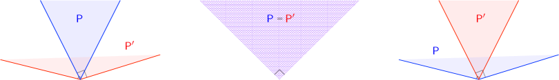
Figure 1: Examples of several cones ${\sf P}$ and their duals ${\sf P}^{\prime}$ in ${\mathbb{R}}^{2}$. Duality is with respect to the standard Euclidean inner product. If the cone is a “right-angled wedge” (center figure), then it is equal to its dual. Otherwise the narrower the cone’s angle, the larger is the dual cone’s angle as the relation (34) implies.

The main tool used in this paper is that of linear-conic duality. To introduce this concept, we first define the notion of a dual cone.

Definition 5.

Let ${\sf P}\subset{\sf V}$ be a (not necessarily convex) cone in a vector space ${\sf V}$. Its dual cone ${\sf P}^{\prime}\subset{\sf V}^{\prime}$ is the set of all linear functionals that are positive on all of ${\sf P}$

$${\sf P}^{\prime}~{}:=~{}\left\{\rule{0.0pt}{9.10004pt}H\in{\sf V}^{\prime};~{}\forall M\in{\sf P},~{}\left<H\bm{,}M\right>\geq 0\right\}.$$ (33)

Figure 1 shows examples of several cones in ${\mathbb{R}}^{2}$. Some cones are “self-dual”, i.e. ${\sf P}^{\prime}={\sf P}$, but most cones in ${\mathbb{R}}^{n}$ are not. An intuitive picture to keep in mind is that the smaller the cone is, the larger is its dual since the requirement (33) that elements of ${\sf P}^{\prime}$ have to satisfy is less stringent the smaller ${\sf P}$ is. Similarly, the larger a cone is, the smaller is its dual. More precisely, it is easy to show from the definition that

$${\sf P}_{1}~{}\subseteq~{}{\sf P}_{2}\hskip 20.00003pt\Leftrightarrow\hskip 20.00003pt{\sf P}_{2}^{\prime}~{}\subseteq~{}{\sf P}_{1}^{\prime}.$$ (34)

Example 6.

Any positive rank-one matrix can be written as $M=vv^{*}$ for some vector $v$. Thus another characterization of the set of positive rank-one matrices is

$$\mathbb{P}_{n}^{1}~{}=~{}\left\{\rule{0.0pt}{9.10004pt}M~{}=~{}vv^{*};~{}v\in{\mathbb{R}}^{n}\right\}.$$

Thus a matrix $H$ in the cone dual to $\mathbb{P}_{n}^{1}$ must satisfy

$$\forall M\in\mathbb{P}_{n}^{1},~{}{\rm tr}\!\left(HM\right)\geq 0\hskip 20.00003pt\Leftrightarrow\hskip 20.00003pt\forall v\in{\mathbb{R}}^{n},~{}{\rm tr}\!\left(Hvv^{*}\right)=v^{*}Hv\geq 0\hskip 20.00003pt\Leftrightarrow\hskip 20.00003ptH\geq 0,$$

i.e. $H\in{\mathbb{P}_{n}^{1}}^{\prime}$ iff $H\in\mathbb{P}_{n}$.

Now to calculate the cone dual to $\mathbb{P}_{n}$, recall the symmetric factorization of any positive matrix $M=UU^{*}$ for some matrix $U$. A matrix $H$ in the cone dual to $\mathbb{P}_{n}$ then must satisfy

$$\forall M\in\mathbb{P}_{n},~{}{\rm tr}\!\left(HM\right)\geq 0\hskip 20.00003pt\Leftrightarrow\hskip 20.00003pt\forall U,~{}{\rm tr}\!\left(HUU^{*}\right)={\rm tr}\!\left(U^{*}HU\right)\geq 0\hskip 20.00003pt\Leftrightarrow\hskip 20.00003ptH\geq 0.$$

We therefore conclude that the dual of either $\mathbb{P}_{n}^{1}$ or $\mathbb{P}_{n}$ is $\mathbb{P}_{n}$. In particular the set of all positive matrices is its own dual.

An interesting observation from the previous calculation is that the dual of the non-convex cone $\mathbb{P}_{n}^{1}$ is the convex cone $\mathbb{P}_{n}$. This turns out to be true in general.

Lemma 7.

Let ${\sf P}\subset{\sf V}$ be a (not-necessarily convex) cone. Its dual ${\sf P}^{\prime}$ is a convex cone in ${\sf V}^{\prime}$. Furthermore, if ${\sf V}$ is finite dimensional, then the “dual of the dual” is the convex hull of the original cone

$$\left({\sf P}^{\prime}\right)^{\prime}~{}=~{}{\sf Conv}\!\left({\sf P}\right)$$

The proof of the first statement is immediate, and is left as an exercise. A good intuition for the second statement is provided by observing that $\left({\sf P}^{\prime}\right)^{\prime}$ must contain ${\sf P}$, but also must be convex (since it’s a dual), and therefore must at least contain the convex hull of ${\sf P}$.

Another simple, but important, property we require is a statement about the image of sets and their convex hulls under linear functionals. Let ${\sf S}\subset{\sf V}$ be any subset of a vector space ${\sf V}$, then the set-of-values over ${\sf S}$ of a linear functional $\left<{\bm{Q}}\bm{,}.\right>:{\sf V}\rightarrow{\mathbb{R}}$ satisfies

$${\sf Conv}\!\left(\left\{\left<{\bm{Q}}\bm{,}X\right>;~{}X\in{\sf S}\rule{0.0pt}{10.00002pt}\right\}\rule{0.0pt}{10.00002pt}\right)~{}=~{}\left\{\left<{\bm{Q}}\bm{,}X\right>;~{}X\in{\sf Conv}\!\left({\sf S}\right)\rule{0.0pt}{10.00002pt}\right\},$$

i.e. the convex hull of the set-of-values over ${\sf S}$ is the set-of-values over the convex hull of ${\sf S}$. This statement follows immediately from the linearity of the functional. In particular, the extrema of any linear functional over non-convex sets are the same as the extrema over their convex hulls

$$\inf_{X\in{\sf S}}\left<{\bm{Q}}\bm{,}X\right>~{}=~{}\inf_{X\in{\sf Conv}\!\left({\sf S}\right)}\left<{\bm{Q}}\bm{,}X\right>,\hskip 20.00003pt\hskip 20.00003pt\sup_{X\in{\sf S}}\left<{\bm{Q}}\bm{,}X\right>~{}=~{}\sup_{X\in{\sf Conv}\!\left({\sf S}\right)}\left<{\bm{Q}}\bm{,}X\right>.$$ (35)

This is useful when checking extremal values of linear functionals over non-convex cones such as $\mathbb{P}_{n}^{1}$.

We are now ready to state the linear-conic duality theorem, which is a minor modification of the general topological vector space case as stated in [29].

Theorem 8 (Weak Linear-Conic Duality).

Let $\mathcal{L}:{\sf V}\rightarrow{\sf V}_{\rm e}$ be a bounded linear operator between Banach spaces, and let ${\sf P}\subset{\sf V}$ be a (not necessarily convex) cone. Denote by $\mathcal{L}^{{\bm{*}}}$, and ${\sf P}^{\prime}\subset{\sf V}^{\prime}$ the adjoint and dual cone respectively. The following optimization problems are duals

$$\inf_{\scriptsize\begin{tabular}[]{r}$\mathcal{L}(X)=B$\\ $X\in{\sf P}$\end{tabular}}\left<Q\bm{,}X\right>\hskip 20.00003pt\geq~{}\sup_{\scriptsize\begin{tabular}[]{r}$Q-\mathcal{L}^{{\bm{*}}}(Y)\in{\sf P}^{\prime}$\\ $Y\in V_{\rm e}^{\prime}$\end{tabular}}\left<Y\bm{,}B\right>~{}=\operatorname*{-~{}inf}_{\scriptsize\begin{tabular}[]{r}$Q+\mathcal{L}^{{\bm{*}}}(Z)\in{\sf P}^{\prime}$\\ $Z\in V_{\rm e}^{\prime}$\end{tabular}}\left<Z\bm{,}B\right>,$$ (36)

If in addition there exists feasible ${\bar{X}}$ and ${\bar{Y}}$ (or ${\bar{X}}$ and ${\bar{Z}}$) that satisfy the complementary slackness (alignment) condition

$$\left<Q-\mathcal{L}^{{\bm{*}}}\big{(}{\bar{Y}}\big{)}\rule{0.0pt}{8.50006pt}\bm{,}{\bar{X}}\right>=0\hskip 20.00003pt\hskip 20.00003pt\big{(}\mbox{or}~{}\left<Q+\mathcal{L}^{{\bm{*}}}\big{(}{\bar{Z}}\big{)}\rule{0.0pt}{8.50006pt}\bm{,}{\bar{X}}\right>=0\big{)},$$ (37)

then the two objectives are equal, and ${\bar{X}}$, ${\bar{Y}}$ (or ${\bar{X}}$, ${\bar{Z}}$) are optimal for the respective problems.

Proof.

The following two functionals are equal whenever $X$ satisfies $B-\mathcal{L}(X)=0$

$$\left<Q\bm{,}X\right>~{} =~{}\left<Q\bm{,}X\right>+\left<Y\bm{,}B-\mathcal{L}(X)\rule{0.0pt}{9.10004pt}\right>~{}=~{}\left<Q\bm{,}X\right>+\left<Y\bm{,}B\right>-\left<Y\bm{,}\mathcal{L}(X)\rule{0.0pt}{9.10004pt}\right>$$

$$=~{}\left<Q\bm{,}X\right>+\left<Y\bm{,}B\right>-\left<\mathcal{L}^{{\bm{*}}}(Y)\bm{,}X\rule{0.0pt}{9.10004pt}\right>~{}=~{}\left<Q-\mathcal{L}^{{\bm{*}}}(Y)\rule{0.0pt}{9.10004pt}\bm{,}X\right>+\left<Y\bm{,}B\right>,$$

where $Y\in{\sf V}_{\rm e}^{\prime}$ represents any linear functional. Thus their infima over any subset of that set are equal. In particular

$$\inf_{\scriptsize\begin{tabular}[]{r}$\mathcal{L}(X)=B$\\ $X\in{\sf P}$\end{tabular}}\left<Q\bm{,}X\right>~{}=~{}\inf_{\scriptsize\begin{tabular}[]{r}$\mathcal{L}(X)=B$\\ $X\in{\sf P}$\end{tabular}}\left<Q-\mathcal{L}^{{\bm{*}}}(Y)\rule{0.0pt}{9.10004pt}\bm{,}X\right>+\left<Y\bm{,}B\right>.$$ (38)

Now if we restrict $Y$ such that $Q-\mathcal{L}^{{\bm{*}}}(Y)\in{\sf P}^{\prime}$, then because $X\in{\sf P}$, we have $\left<Q-\mathcal{L}^{{\bm{*}}}(Y)\rule{0.0pt}{9.10004pt}\bm{,}X\right>\geq 0$, and therefore a lower bound on the right hand side

$$\inf_{\scriptsize\begin{tabular}[]{r}$\mathcal{L}(X)=B$\\ $X\in{\sf P}$\end{tabular}}\left<Q-\mathcal{L}^{{\bm{*}}}(Y)\rule{0.0pt}{9.10004pt}\bm{,}X\right>+\left<Y\bm{,}B\right>~{}~{}\geq~{}~{}\left<Y\bm{,}B\right>,\hskip 20.00003pt\mbox{for}~{}Q-\mathcal{L}^{{\bm{*}}}(Y)\in{\sf P}^{\prime}.$$ (39)

Replacing the right hand side with its supremum over the set of constrained $Y$’s, and replacing the left hand side with the left hand side of (38), we get the desired inequality

$$\inf_{\footnotesize\begin{tabular}[]{r}$\mathcal{L}(X)=B$\\ $X\in{\sf P}$\end{tabular}}\left<Q\bm{,}X\right>~{}~{}\geq~{}~{}\sup_{\footnotesize\begin{tabular}[]{r}$Q-\mathcal{L}^{{\bm{*}}}(Y)\in{\sf P}^{\prime}$\end{tabular}}\left<Y\bm{,}B\right>.$$

Finally observe that if there is feasible pair $({\bar{X}},{\bar{Y}})$ satisfying the alignment condition (37), then the inequality (39) becomes an equality, and the two problems have equal optimal values of the objectives.

The statement for the problem with the variable $Z$ follows from replacing $Y$ by $-Z$ in the supremum version of the dual problem. ∎

2.5 Schur Complements

Given any Hermitian matrix $M$, it defines a quadratic form ${\sf q}(v):=\left<v\bm{,}Mv\right>$. The matrix is positive definite (semi-definite) if the quadratic form is positive (semi-definite) for all non-zero vectors. If the underlying vector space is transformed by a linear transformation $v=Tw$, then

$${\sf q}(v)~{}=~{}\left<v\bm{,}Mv\right>~{}=~{}\left<Tw\bm{,}MTw\right>~{}=~{}\left<w\bm{,}T^{*}MTw\right>.$$

The transformation $M\mapsto T^{*}MT$ is a congruence transformation on the matrix $M$. Thus under a change of basis, matrix representations of bilinear forms undergo congruence transformations. Consequently, congruence transformations preserve the sign definiteness of a Hermitian matrix. They also preserve its “inertia”, namely the triple of numbers indicating the number of negative, zero, and positive eigenvalues respectively.

The well-known Schur complement can be understood as block-diagonalizatoin by a congruence transformation on a $2\times 2$-block partitioned matrix. Consider a Hermitian matrix $M$ partitioned as

$$M~{}=~{}\begin{bmatrix}M_{11}&M_{\rm o}\\ M_{\rm o}^{*}&M_{22}\end{bmatrix}.$$

If $M_{22}$ is invertible, then $M$ can be block-diagonalized by the following congruence transformation

$$\begin{bmatrix}M_{11}&M_{\rm o}\\ M_{\rm o}^{*}&M_{22}\end{bmatrix}~{}=~{}\begin{bmatrix}I&M_{\rm o}M_{22}^{-1}\\ 0&I\end{bmatrix}\begin{bmatrix}M_{11}-M_{\rm o}M_{22}^{-1}M_{\rm o}^{*}&0\\ 0&M_{22}\end{bmatrix}\begin{bmatrix}I&0\\ M_{22}^{-1}M_{\rm o}^{*}&I\end{bmatrix}.$$ (40)

We can therefore immediately conclude that if $M_{22}>0$, then $M\geq 0$ iff the Schur complement $M_{11}-M_{\rm o}M_{22}^{-1}M_{\rm o}^{*}\geq 0$. This is particularly useful if for example $M_{22}$ is fixed, and the other blocks of $M$ contain a matrix variable such as might occur in a Linear Matrix Inequality (LMI). In this case, positivity of the Schur complement gives another matrix inequality (a “Riccati inequality”, not an LMI) which can be more useful as we will see in the next section.

3 DLMIs, DRIs and DREs

In this section we explore the relationships between Differential Linear Matrix Inequalities (DLMIs), Differential Riccati Inequalities (DRIs) and Differential Riccati Equations (DREs). To begin with, we recall some fundamental facts about the simplest of DLMIs, namely Differential Lyapunov Inequalities, and then apply those to compare solutions of Riccati differential equations in terms of their coefficients’ differences. The exposition here is intended to be self contained.

Differential Lyapunov Inequalities

Consider a differential Lyapunov inequality of the form

$$\dot{X}+F^{*}X+XF~{}\leq~{}0,\hskip 20.00003ptt\in[0,{\scriptstyle T}],\hskip 20.00003pt\begin{array}[]{rcl}X(0)&=&0,\\ \mbox{or}~{}X({\scriptstyle T})&=&0.\end{array}$$ (41)

There are many solutions to such a differential inequality, but they all have a sign definiteness depending on whether initial or final conditions are given. The key to understanding the inequality (41) is to recast it as an equality with a “forcing term” as follows

$$\dot{X}+F^{*}X+XF~{}\leq~{}0\hskip 20.00003pt \Leftrightarrow\hskip 20.00003pt\dot{X}+F^{*}X+XF~{}=~{}-H, H(t)\geq 0,$$

$$\Leftrightarrow\hskip 20.00003pt-\dot{X}=F^{*}X+XF+H, H(t)\geq 0,$$ (42)

where $H$ is an arbitrary positive matrix-valued function. Equation (42) is a differential Lyapunov equation which has the following solutions depending on whether final or initial time conditions are given

$$-\dot{X}=F^{*}X+XF+H,\hskip 10.00002ptX(0)=0 \Rightarrow\hskip 20.00003ptX(t)=-\scaleobj{.8}{\int_{{0}}^{{t}}}\Phi^{*}(t,\tau)H(\tau)\Phi(t,\tau)~{}d\tau,$$ (43)

$$-\dot{X}=F^{*}X+XF+H,\hskip 10.00002ptX({\scriptstyle T})=0 \Rightarrow\hskip 20.00003ptX(t)=\scaleobj{.8}{\int_{{t}}^{{T}}}\Phi^{*}(t,\tau)H(\tau)\Phi(t,\tau)~{}d\tau,$$ (44)

where $\Phi$ is a state-transition matrix of $F$ such that $(d/dt)\Phi(t,\tau)=\Phi(t,\tau)F(t)$.

Note that the definiteness of $X$ is determined by the definiteness of $H$ in (43) or (44). Combining this with (42), we conclude that

$$\dot{X}+F^{*}X+XF~{}\leq~{}0,\hskip 20.00003pt\begin{array}[]{lcl}X(0)=0&\hskip 20.00003pt\Rightarrow&X(t)\leq 0,\hskip 10.00002ptt\in[0,{\scriptstyle T}],\\ X({\scriptstyle T})=0&\hskip 20.00003pt\Rightarrow&X(t)\geq 0,\hskip 10.00002ptt\in[0,{\scriptstyle T}].\end{array}$$ (45)

A useful intuition to keep in mind is that $\dot{X}\leq-F^{*}X-XF$ indicates that $X$ will start as negative if propagated forward from $X(0)=0$. For backwards propagation from $X({\scriptstyle T})=0$, the derivative “looking backwards” is $-\dot{X}$, and the inequality $-\dot{X}\geq-F^{*}X-XF$ impies that $X$ should start as positive when propagated backwards from zero final condition. Finally, note that because a state-transition matrix is always full rank, the expressions (43) and (44) imply inequalities can be replaced by strict inequalities in (45).

Differential Riccati Inequalities and Riccati Comparisons

By adding a quadratic and a constant term to the differential Lyapunov inequality, we obtain a Differential Riccati Inequality (DRI) which is of the form

$$\dot{\Lambda}+A^{*}\Lambda+\Lambda A-\Lambda~{}M~{}\Lambda+Q~{}\geq~{}0,\hskip 20.00003pt\Lambda({\scriptstyle T})=0.$$ (46)

For simplicity of exponsition, the DRI here is stated for the inequality $\geq$ and a final condition. Similar DRIs can be obtained by using combinations of $\geq,\leq$ and final or initial conditions.

The DRI (46) has many solutions, but there is a maximal solution which has special properties as is described next. In a manner similar to what was done for Lyapunov inequalities, the DRI (46) can be recast as a Differential Riccati Equation (DRE) with an arbitrary positive “forcing” term $H$

$$\dot{\Lambda}+A^{*}\Lambda+\Lambda A-\Lambda~{}M~{}\Lambda+Q~{} =~{}H~{}\geq~{}0,\hskip 20.00003pt\Lambda({\scriptstyle T})=0,$$

$$\Rightarrow\hskip 20.00003pt\dot{\Lambda}+A^{*}\Lambda+\Lambda A-\Lambda~{}M~{}\Lambda+Q-H~{} =~{}0,\hskip 20.00003ptH\geq 0,\hskip 20.00003pt\Lambda({\scriptstyle T})=0.$$ (47)

Thus given any solution $\Lambda$ of the DRI (46), there exists a positive matrix-valued function $H$ such that $\Lambda$ is a solution of the DRE (47) and vice versa.

Some intuition for (47) can be obtained by rewriting it as follows

$$-\dot{\Lambda}~{}=~{}A^{*}\Lambda+\Lambda A-\Lambda~{}M~{}\Lambda+Q-H,\hskip 20.00003ptH\geq 0,\hskip 20.00003pt\Lambda({\scriptstyle T})=0.$$

Suppose the equation is solved “backwards” from the final condition over $[0,{\scriptstyle T}]$. The quantity $-{\dot{\Lambda}}(t)$ is the derivative “looking backwards”. Compared with the choice $H(t)=0$, that backwards derivative can only be smaller with a choice of $H(t)\geq 0$. Therefore the solution with $H(t)=0$ should be the largest of all solutions with $H(t)\geq 0$. Figure 2 shows simulations with a scalar example where the function $H$ was chosen as a positive random number switching at ten different points in an interval $[0,{\scriptstyle T}]$. One hundred such solutions are shown. In addition, the solution with $H(t)=0$ is also shown, and it appears to be the maximum of all the other solutions. We can show that this behavior is true in general using the previous results on Lyapunov inequalities as shown next.

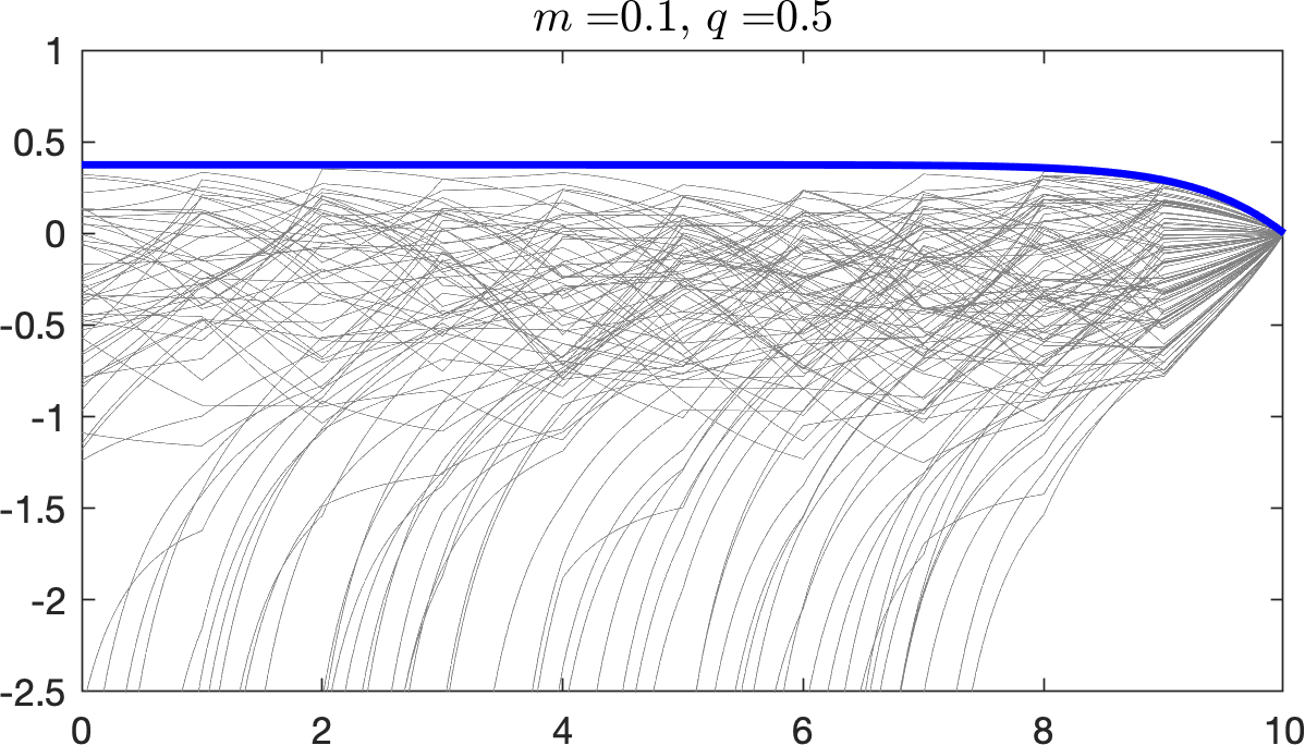
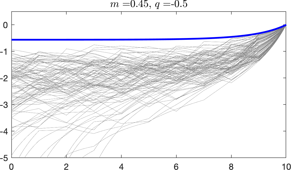
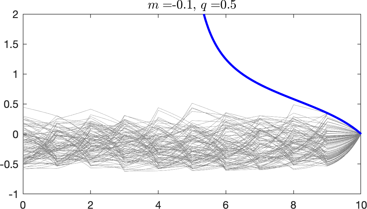
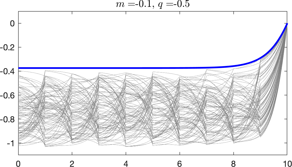
Figure 2: Examples demonstrating the maximal property of the solution ${\bar{\Lambda}}$ of the Differential Riccati Equation (DRE) with final conditions (49) over all possible solutions of the Differential Riccati Inequality (DRI) (48). The equation here is scalar ($n=1$), and therefore becomes $-\dot{{\bar{\lambda}}}(t)=q+2a{\bar{\lambda}}(t)-m{\bar{\lambda}}^{2}(t)$, and various combinations of the signs of $q$ and $m$ are given. The gray curves represent 100 different solutions of the DRI, while the thick blue curve is the solution of the DRE. Notice how the maximality property is maintained even when the DRE and/or DRI solutions have finite escape time.

Lemma 9 (Maximal Solutions of DRIs).

Consider the final-condition Differential Riccati Inequality (DRI)

$${\dot{\Lambda}}+A^{*}\Lambda+\Lambda A-\Lambda M\Lambda+Q~{}\geq~{}0,\hskip 20.00003pt\hskip 20.00003pt\Lambda({\scriptstyle T})=\Lambda_{\rm f}.$$ (48)

The maximal solution of the DRI is given by the following Differential Riccati Equation (DRE)

$$\dot{{\bar{\Lambda}}}+A^{*}{\bar{\Lambda}}+{\bar{\Lambda}}A-{\bar{\Lambda}}M{\bar{\Lambda}}+Q~{}=~{}0,\hskip 20.00003pt\hskip 20.00003pt{\bar{\Lambda}}(T)=\Lambda_{\rm f},$$ (49)

i.e. for any other $\Lambda$ satisfying the DRI,

$${\bar{\Lambda}}(t)~{}\geq~{}\Lambda(t),\hskip 20.00003ptt\in[0,{\scriptstyle T}].$$

Note that this statement says nothing about minimal solutions to final value problems. Indeed, as shown by the examples in Figure 2, there may not exist such solutions.

Before proving this statement, we recap a “Riccati comparison” result which is a finite-horizon version of a classic infinite-horizon argument [5, Lemma 3]. Consider solutions of two Riccati differential equations with different “$Q$-terms”

$$0{} =~{}{\dot{\Lambda}}_{1}+A^{*}\Lambda_{1}+\Lambda_{1}A-\Lambda_{1}M\Lambda_{1}+Q_{1},\hskip 20.00003pt\Lambda_{1}({\scriptstyle T})=\Lambda_{{\rm f}},$$ (50)

$$0{} =~{}{\dot{\Lambda}}_{2}+A^{*}\Lambda_{2}+\Lambda_{2}A-\Lambda_{2}M\Lambda_{2}+Q_{2},\hskip 20.00003pt\Lambda_{2}({\scriptstyle T})=\Lambda_{\rm f},$$

with $Q_{1}\geq Q_{2}$. Define the difference ${\tilde{\Lambda}}:=\Lambda_{1}-\Lambda_{2}$, subtract the two equations and apply the Riccati difference formula (98) to obtain

$$\dot{{\tilde{\Lambda}}}+\left(A+M\big{(}\Lambda_{1}+\Lambda_{2}\big{)}/2\right)^{*}{\tilde{\Lambda}}+{\tilde{\Lambda}}\left(A+M\big{(}\Lambda_{1}+\Lambda_{2}\big{)}/2\right)+\left(Q_{1}-Q_{2}\right)~{} =~{}0,\hskip 20.00003pt\hskip 20.00003pt{\tilde{\Lambda}}({\scriptstyle T})=0$$

$$\Rightarrow\hskip 20.00003pt\dot{{\tilde{\Lambda}}}+\left(A+M\big{(}\Lambda_{1}+\Lambda_{2}\big{)}/2\right)^{*}{\tilde{\Lambda}}+{\tilde{\Lambda}}\left(A+M\big{(}\Lambda_{1}+\Lambda_{2}\big{)}/2\right)~{} =~{}-\left(Q_{1}-Q_{2}\right)~{}\leq~{}0.$$

This is a differential Lyapunov inequality of the form (41) for ${\tilde{\Lambda}}$. Applying (45) we conclude that ${\tilde{\Lambda}}(t)\geq 0$, and thus for the differential Riccati equations (50) with final conditions

$$Q_{1}(t)\geq Q_{2}(t),\hskip 10.00002ptt\in[0,{\scriptstyle T}]\hskip 20.00003pt\Rightarrow\hskip 20.00003pt\Lambda_{1}(t)\geq\Lambda_{2}(t),\hskip 10.00002ptt\in[0,{\scriptstyle T}].$$ (51)

Note that properties of $M$ (such as sign definiteness) play no role in the arguments above.

Proof.

(of Lemma 9). Consider the DRI (48) rewritten with the “forcing variable” $H\geq 0$, and the DRE (49) obtained from it by setting the inequality to equality

$$\dot{\Lambda}+A^{*}\Lambda+\Lambda A-\Lambda~{}M~{}\Lambda+Q~{}\geq~{}0\hskip 20.00003pt\Leftrightarrow\hskip 20.00003pt\dot{\Lambda}+A^{*}\Lambda+\Lambda A-\Lambda~{}M~{}\Lambda+(Q-H)~{} =~{}0,\hskip 20.00003ptH\geq 0,$$

$$\dot{{\bar{\Lambda}}}+A^{*}{\bar{\Lambda}}+{\bar{\Lambda}}A-{\bar{\Lambda}}~{}M~{}{\bar{\Lambda}}+Q~{} =~{}0.$$

Since $H\geq 0$, then $Q\geq(Q-H)$, and the Riccati comparison result (51) implies that

$${\bar{\Lambda}}(t)~{}\geq~{}\Lambda(t),\hskip 20.00003ptt\in[0,{\scriptstyle T}].\qed$$

Differential Linear Matrix Inequalities (DLMIs)

We are concerned with Differential Linear Matrix Inequalities (DLMIs) of a very special form where a matrix-valued function $\Lambda(.)$ is required to satisfy

$${\cal M}({\color[rgb]{0,0,1}{\Lambda}})~{}:= ~{}{\bm{Q}}+{\mathcal{E}}^{{\bm{*}}}(\dot{{\color[rgb]{0,0,1}{\Lambda}}})+\mathcal{A}^{{\bm{*}}}({\color[rgb]{0,0,1}{\Lambda}})$$

$$~{}:= ~{}\begin{bmatrix}Q&N\\ N^{*}&R\end{bmatrix}+\begin{bmatrix}I\\ 0\end{bmatrix}{\color[rgb]{0,0,1}{\dot{\Lambda}}}\begin{bmatrix}I&0\end{bmatrix}+\begin{bmatrix}A^{*}\\ B^{*}\end{bmatrix}{\color[rgb]{0,0,1}{\Lambda}}\begin{bmatrix}I&0\end{bmatrix}+\begin{bmatrix}I\\ 0\end{bmatrix}{\color[rgb]{0,0,1}{\Lambda}}\begin{bmatrix}A&B\end{bmatrix}$$

$$= ~{}\begin{bmatrix}Q+\dot{{\color[rgb]{0,0,1}{\Lambda}}}+A^{*}{\color[rgb]{0,0,1}{\Lambda}}+{\color[rgb]{0,0,1}{\Lambda}}A&N+{\color[rgb]{0,0,1}{\Lambda}}B\\ (N+{\color[rgb]{0,0,1}{\Lambda}}B)^{*}&R\end{bmatrix}~{}\geq~{}0,\hskip 20.00003pt\hskip 20.00003ptt\in[0,{\scriptstyle T}].$$ (52)

Even when boundary conditions for $\Lambda$ are specified, such DLMIs typically have non-unique solutions. In other words, the inequality above does not provide sufficient constraints to uniquely determined ${\dot{\Lambda}}(t)$ given $\Lambda(t)$, thus the non-uniqueness of solutions. However, as in the case of Riccati inequalities, we are able to find maximal solutions of the DLMI by relating it to a DRI via the Schur complement. For notational simplicity, the statements in this section are presented for the case $N=0$. The general case is given in Theorem 14 of Appendix A.5.

Since the matrix ${\cal M}(\Lambda)$ is in a $2\times 2$-block partition, it is natural to use the Schur complement to characterize its positivity. First note that $R\geq 0$ is a necessary condition for (52). If we further assume that $R>0$, then the Schur complement (40) gives the congruence

$$\begin{bmatrix}Q+\dot{\Lambda}+A^{*}\Lambda+\Lambda A&\Lambda B\\ B^{*}\Lambda&R\end{bmatrix}=\begin{bmatrix}I&\Lambda BR^{-1}\\ 0&I\end{bmatrix}\begin{bmatrix}Q+\dot{\Lambda}+A^{*}\Lambda+\Lambda A-\Lambda~{}BR^{\text{-}1}B^{*}~{}\Lambda&0\\ 0&R\end{bmatrix}\begin{bmatrix}I&0\\ R^{-1}B^{*}\Lambda^{*}&I\end{bmatrix}$$ (53)

Thus the DLMI is equivalent to the DRI

$$Q+\dot{\Lambda}+A^{*}\Lambda+\Lambda A-\Lambda~{}BR^{\text{-}1}B^{*}~{}\Lambda~{}\geq~{}0.$$

Furthermore, if we have final conditions on the DLMI, then the equivalent DRI is of the form (46). Therefore the previously stated facts about maximal solutions apply. In addition, the left-hand-side of (53) implies that the lowest rank possible for the DLMI matrix is bounded from below by the rank of $R$. The right-hand-side of (53) shows that this minimum ranks is achieved by setting the inequality in the DRI to equality (which renders the $(1,1)$ as zero). This gives a special symmetric factorization of the DLMI matrix at the maximal solution as stated next.

Lemma 10.

(Maximal Solutions of the DLMI) Consider the final-value DLMI and its associated DRI

$$\begin{aligned} {\cal M}(\Lambda)&:={\bm{Q}}+{\mathcal{E}}^{{\bm{*}}}({\dot{\Lambda}})+\mathcal{A}^{{\bm{*}}}(\Lambda)=\begin{bmatrix}Q+\dot{\Lambda}+A^{*}\Lambda+\Lambda A&\Lambda B\\ B^{*}\Lambda&R\end{bmatrix}\geq~{}0,\\ \mathcal{R}(\Lambda)&:={\dot{\Lambda}}+A^{*}\Lambda+\Lambda A-\Lambda BR^{\text{-}1}B^{*}\Lambda+Q~{}\geq~{}0,\end{aligned}\hskip 20.00003ptt\in[0,{\scriptstyle T}],\hskip 20.00003pt\Lambda({\scriptstyle T})=\Lambda_{\rm f},$$

where $R>0$. A maximal solution of either inequality is given by the Differential Riccati Equation (DRE)

$$\dot{{\bar{\Lambda}}}+A^{*}{\bar{\Lambda}}+{\bar{\Lambda}}A-{\bar{\Lambda}}BR^{\text{-}1}B^{*}{\bar{\Lambda}}+Q~{}=~{}0,\hskip 20.00003pt\hskip 20.00003pt{\bar{\Lambda}}(T)=\Lambda_{\rm f},$$ (54)

i.e. for any other $\Lambda$ satisfying the DLMI or equivalently the DRI, ${\bar{\Lambda}}(t)~{}\geq~{}\Lambda(t),~{}t\in[0,{\scriptstyle T}].$ Furthermore, at the maximal solution, the matrix ${\cal M}({\bar{\Lambda}})$ has the full-rank symmetric factorization

$${\cal M}({\bar{\Lambda}})~{}=~{}\begin{bmatrix}{\bar{\Lambda}}BR^{\text{-}\frac{1}{2}}\\ R^{\frac{1}{2}}\end{bmatrix}\begin{bmatrix}R^{\text{-}\frac{1}{2}}B^{*}{\bar{\Lambda}}&R^{\frac{1}{2}}\end{bmatrix}.$$ (55)

Proof.

Note that the equivalences of the DREs and the DLMIs follow from the Schur complements for $R>0$. Thus showing the maximality property for the DRIs (already shown in Lemma 9) proves the maximality property for the DLMIs.

For the factorization (55), note that if ${\bar{\Lambda}}$ which satisfies the DRE is used in both sides of (53)

$$\begin{bmatrix}Q+\dot{{\bar{\Lambda}}}+A^{*}{\bar{\Lambda}}+{\bar{\Lambda}}A&{\bar{\Lambda}}B\\ B^{*}{\bar{\Lambda}}&R\end{bmatrix}~{} =~{}\begin{bmatrix}{\bar{\Lambda}}BR^{-1}\\ I\end{bmatrix}R\begin{bmatrix}R^{-1}B^{*}{\bar{\Lambda}}^{*}&I\end{bmatrix}~{}=~{}\begin{bmatrix}{\bar{\Lambda}}BR^{\text{-}\frac{1}{2}}\\ R^{\frac{1}{2}}\end{bmatrix}\begin{bmatrix}R^{\text{-}\frac{1}{2}}B^{*}{\bar{\Lambda}}B&R^{\frac{1}{2}}\end{bmatrix},$$

which is a full-rank factorization since $R$ (and therefore $R^{\frac{1}{2}}$) is assumed non-singular. ∎

A few remarks are needed to emphasize the implications of the above result.

• The symmetric factorization (55) implies that the rank of ${\cal M}(.)$ at the extremum ${\bar{\Lambda}}$ is exactly equal the rank of $R$. Since we have assumed $R$ is non-singular, then this is the lowest rank ${\cal M}(.)$ can be. We therefore conclude that the DRE solution also minimizes the rank of the DLMI matrix ${\cal M}(\Lambda)$. This fact will be important for understanding the structure of optimal signals later on, as it will imply the specific state feedback form of optimal inputs.

• Another important point to reiterate here is that one needed to convert a DLMI to a DRI in order to find extremal solutions by substituting equality for inequality in the DRIs. It is not possible to find maximal solutions of the DLMIs directly by changing their inequalities to equalities. The DLMI with equality is infeasible (it would imply for example that $R=0$). The DLMI and the DRI are equivalent by the Schur complement, but changing the inequalities to equalities does not maintain that equivalence. Thus to find maximal solutions to a DLMI, one must convert it to the equivalent DRI, and then set the latter to equality.

Symmetric Factorizations and the Lur’e Equations

As an aside, we point out that the factorization (55) indicates another route that can be taken to arrive at the DRE starting from the DLMI without using the Schur complement. Observe that a matrix $M$ is positive iff it has a symmetric factorization of the form $M=UU^{*}$ for some matrix $U$. Consider any such factorization of ${\cal M}(\Lambda)$ which is partitioned conformably as

$${\cal M}(\Lambda)~{}:=~{}\begin{bmatrix}Q+\dot{\Lambda}+A^{*}\Lambda+\Lambda A&(N+\Lambda B)\\ (N+\Lambda B)^{*}&R\end{bmatrix}~{}=~{}\begin{bmatrix}U_{1}\\ U_{2}\end{bmatrix}\begin{bmatrix}U_{1}^{*}&U_{2}^{*}\end{bmatrix}~{}=:~{}UU^{*}.$$ (56)

This gives the following constraints on the submatrices $U_{1}$ and $U_{2}$

$$U_{1}U_{1}^{*}=Q+\dot{\Lambda}+A^{*}\Lambda+\Lambda A,\hskip 20.00003ptU_{1}U_{2}^{*}=N+\Lambda B,\hskip 20.00003ptU_{2}U_{2}^{*}=R.$$ (57)

These equations are the time-varying version of what are sometimes referred to as Lur’e equations, which are normally stated as follows. Given $A,B,Q,N,R$, find matrices $\Lambda$, $U_{1}$ and $U_{2}$ such that the equations (57) hold. In our current language, this amounts to finding $\Lambda$ such that ${\cal M}(\Lambda)\geq 0$, as well as a symmetric factorization of ${\cal M}(\Lambda)$. Such symmetric factorizations always exist for any positive matrix ${\cal M}(\Lambda)$.

If $R>0$, then the factorization $R=U_{2}U_{2}^{*}$ implies that $U_{2}$ has full row rank. The “tightest” such factorization would have $U_{2}$ to be square. This corresponds to the factorization (56) being full rank, which is also the minimal rank that the factor $U$ can have. Thus, if $R>0$, and we adopt a full-rank factorization in (56), then $U_{2}$ is square and invertible, which gives $U_{1}=\Lambda BU_{2}^{-*}$, and in turn

$$U_{1}U_{1}^{*}~{}=~{}\Lambda BU_{2}^{-*}U_{2}^{-1}B^{*}\Lambda~{}=~{}\Lambda B\left(U_{2}U_{2}^{*}\right)^{-1}B^{*}\Lambda~{}=~{}\Lambda BR^{\text{-}1}B^{*}\Lambda.$$

Substituting this in the first equation in (57) gives the DRE

$$\Lambda BR^{-1}B^{*}\Lambda=Q+\dot{\Lambda}+A^{*}\Lambda+\Lambda A.$$

Thus we see that the DRE arises out of a full-rank factorization of the DLMI matrix (56), or equivalently, a minimal-rank (of $U$) solution to the Lur’e equations. The Schur complement is not used in this argument.

4 The Deterministic LQR Problem

Now we apply the procedure outlined in Section 1.2 to the classic Linear Quadratic Regulator (LQR) problem in its deterministic form. Note that in the finite time-horizon case, all statements given below are applicable to time-invariant or time-varying systems and performance objectives provided that the matrix-valued function ${\bm{Q}}(.)$ is bounded. For notational simplicity again, we consider the case with no cross terms $N=0$. The general case follows from Theorem 12 in a later section.

Theorem 11.

Consider a linear (possibly time-varying) system of the form

$$\dot{x}~{}=~{}Ax~{}+~{}Bu,\hskip 20.00003pt\hskip 20.00003ptt\in[0,{\scriptstyle T}],\hskip 20.00003ptx(0)={\rm x}_{\rm i},$$ (58)

and a quadratic form defined on $(x,u)$ pairs

$${\mbox{\large$\mathbf{q}$}}(x,u)~{}:=~{}\int_{0}^{{\scriptscriptstyle T}}\begin{bmatrix}x\\ u\end{bmatrix}^{*}\!\begin{bmatrix}Q&0\\ 0&R\end{bmatrix}\begin{bmatrix}x\\ u\end{bmatrix}dt~{}=:\int_{0}^{{\scriptscriptstyle T}}\begin{bmatrix}x\\ u\end{bmatrix}^{*}\!{\begin{bmatrix}&&\\ &{\bm{Q}}&\\ &&\end{bmatrix}}\begin{bmatrix}x\\ u\end{bmatrix}dt~{}=:\int_{0}^{{\scriptscriptstyle T}}{\sf q}(x,u)~{}dt,$$

with $Q\geq 0$ and $R>0$.

The infimum of the quadratic form $\mathbf{q}$ subject to the constraints (58) is

$$\inf_{x,u}~{}{\mbox{\large$\mathbf{q}$}}(x,u)~{}=~{}{\rm x}_{\rm i}^{*}~{}{\bar{\Lambda}}(0)~{}{\rm x}_{\rm i},$$ (59)

where ${\bar{\Lambda}}$ is the maximal solution of the Differential Linear Matrix Inequality (DLMI) over $[0,{\scriptstyle T}]$

$${\cal M}(\Lambda):={\bm{Q}}+\begin{bmatrix}{\dot{\Lambda}}+A^{*}\Lambda+\Lambda A&\Lambda B\\ B^{*}\Lambda&0\end{bmatrix}~{}\geq~{}0,\hskip 20.00003pt\Lambda({\scriptstyle T})=0.$$ (60)

The maximal solution of this DLMI is given by the solution of the Differential Riccati Equation (DRE)

$$Q+\dot{{\bar{\Lambda}}}+A^{*}{\bar{\Lambda}}+{\bar{\Lambda}}A-{\bar{\Lambda}}BR^{\text{-}1}B^{*}{\bar{\Lambda}}=0,\hskip 20.00003pt\hskip 20.00003pt{\bar{\Lambda}}({\scriptstyle T})=0.$$

The optimal control ${\bar{u}}$ is given by the state feedback law

$${\bar{u}}(t)=\left(R^{\text{-}1}(t)B^{*}(t){\bar{\Lambda}}(t)\rule{0.0pt}{10.00002pt}\right)~{}{\bar{x}}(t),\hskip 20.00003ptt\in[0,{\scriptstyle T}].$$

As outlined in the introduction, we will give the proof of this Theorem in several steps. Step (1) is to reformulate the minimization problem in terms of covariance matrices, which yields a linear-linear optimization problem with a cone constraint. Step (2) is to use conic duality to reformulate it as a maximization problem with a Differential Linear Matrix Inequality (DLMI) constraint. Step (3) is to use the maximal solution of the DLMI (which is given by a DRE) to solve the dual problem. Finally, step (4) uses the alignment (complementary slackness) conditions to give the optimal primal solution in the form of a state feedback and show that the duality gap is zero.

1. The first step is to define the joint (deterministic) covariance of $x$ and $u$

   $$\Sigma(t)~{}:=~{}\begin{bmatrix}x(t)\\ u(t)\end{bmatrix}\begin{bmatrix}x^{*}(t)&u^{*}(t)\end{bmatrix},$$ (61)

   which is always of rank one. The differential equation for $\Sigma$ is (8), which we recap for clarity and rewrite it in the abstract integral form (30) developed in Section 2.2

   $${\mathcal{E}}\big{(}\Sigma\big{)}:=\begin{bmatrix}I&0\end{bmatrix}{\Sigma}\begin{bmatrix}I\\ 0\end{bmatrix},\hskip 20.00003pt \mathcal{A}\big{(}\Sigma\big{)}:=\begin{bmatrix}A&B\end{bmatrix}{\Sigma}\begin{bmatrix}I\\ 0\end{bmatrix}+\begin{bmatrix}I&0\end{bmatrix}{\Sigma}\begin{bmatrix}A^{*}\\ B^{*}\end{bmatrix},$$

   $$\left.\begin{array}[]{rcl}{\mathcal{E}}\big{(}\dot{\Sigma}\big{)}&=&\mathcal{A}\big{(}\Sigma\big{)},\\ {\mathcal{E}}\big{(}\Sigma(0)\big{)}&=&{\rm x}_{\rm i}{\rm x}_{\rm i}^{*}=:{\sf X}_{\rm i}\end{array}\right\}\hskip 20.00003pt \Leftrightarrow\hskip 20.00003pt\big{(}{\mathcal{E}}-{\sf{\bm{I}}}_{\sf f}\mathcal{A}\big{)}(\Sigma)~{}=~{}{\sf X}_{\rm i}.$$ (64)

   Now the LQR problem can be written in the covariance representation as

   $$\boxed{\begin{aligned} \inf_{\Sigma\in{{\sf L}}^{\!1}(0,T)}&\int_{0}^{T}{\rm tr}\!\left({\bm{Q}}~{}\Sigma\right)~{}dt\hskip 100.00015pt&\framebox{\sf Primal: LQR}\\ \big{(}{\mathcal{E}}-{\sf{\bm{I}}}_{\sf f}\mathcal{A}\big{)}(\Sigma)&={\sf X}_{\rm i}\\ \Sigma\geq 0,~{}{\rm\bf rk}\!\left(\Sigma\right)&=1.\end{aligned}~{}}$$ (65)

2. This problem is in the form to which the linear-conic duality Theorem 8 can be applied. The primal and dual problems are then

   $${\sf Primal:}\left\{\begin{array}[]{ccc}{\begin{array}[]{rcl}\displaystyle\inf_{\Sigma\in{{\sf L}}^{\!1}(0,{\scriptscriptstyle T})}&&\left<{\bm{Q}}\bm{,}\Sigma\right>\\ \big{(}{\mathcal{E}}-{\sf{\bm{I}}}_{\sf f}\mathcal{A}\big{)}(\Sigma)&=&{\sf X}_{\rm i}\rule{0.0pt}{15.00002pt}\\ \Sigma\geq 0,~{}{\rm\bf rk}\!\left(\Sigma\right)&=&1\end{array}}&\geq&{\begin{array}[]{rcl}\displaystyle\sup_{Y\in{{\sf L}}^{\!\!\infty}(0,{\scriptscriptstyle T})}&&\left<Y\bm{,}{\sf X}_{\rm i}\right>\\ {\bm{Q}}-\big{(}{\mathcal{E}}^{{\bm{*}}}-\mathcal{A}^{{\bm{*}}}{\sf{\bm{I}}}_{\sf\bm{b}}\big{)}(Y)&\geq&0\rule{0.0pt}{15.00002pt}\end{array}}\end{array}\right\}{\sf:Dual},$$ (66)

   where we recall the calculation of the adjoint of the linear operator in the equality constraint

   $$\big{(}{\mathcal{E}}-{\sf{\bm{I}}}_{\sf f}\mathcal{A}\big{)}^{{\bm{*}}}~{}=~{}{\mathcal{E}}^{{\bm{*}}}-\mathcal{A}^{{\bm{*}}}{\sf{\bm{I}}}_{\sf f}^{{\bm{*}}}~{}=~{}{\mathcal{E}}^{{\bm{*}}}-\mathcal{A}^{{\bm{*}}}{\sf{\bm{I}}}_{\sf\bm{b}}.$$ (67)

   Note that the rank condition does not have any effect on the dual problem. This is of course because the cone dual to positive rank-one matrices $\mathbb{P}_{n}^{1}$ is the convex cone $\mathbb{P}_{n}$ of positive matrices, i.e. the dual problem is always convex even if the primal problem is not. Furthermore, since the cost objective is linear, the argument in (35) implies that the extrema are achieved at the “vertices” of the convex cone.

   Examining the dual objective $\left<Y\bm{,}{\sf X}_{\rm i}\right>$, we see that since ${\sf X}_{\rm i}$ is a constant function over $[0,{\scriptstyle T}]$, the objective can be simplified by introducing the backwards integral of $Y$ as follows

   $$\left<Y\bm{,}{\sf X}_{\rm i}\right>~{}=~{}\scaleobj{.8}{\int_{{0}}^{{T}}}{\rm tr}\!\left(Y(t)~{}{\sf X}_{\rm i}\rule{0.0pt}{10.00002pt}\right)~{}dt~{}=~{}{\rm tr}\!\left(\scaleobj{.8}{\int_{{0}}^{{T}}}Y(t)dt~{}{\sf X}_{\rm i}\right)~{}=:~{}{\rm tr}\!\left(\Lambda(0)~{}{\rm x}_{\rm i}{\rm x}_{\rm i}^{*}\rule{0.0pt}{10.00002pt}\right)~{}=~{}{\rm x}_{\rm i}^{*}\Lambda(0)~{}\!{\rm x}_{\rm i},$$

   where we defined $\Lambda$ as the backwards integral of $Y$

   $$\Lambda:={\sf{\bm{I}}}_{\sf\bm{b}}Y\hskip 20.00003pt\Leftrightarrow\hskip 20.00003pt\left\{\begin{array}[]{rcl}\Lambda(t)&:=&\int_{t}^{T}Y(\tau)~{}d\tau\\ -\dot{\Lambda}(t)&:=&Y(t)\end{array}\right\}\hskip 20.00003pt\Leftrightarrow\hskip 20.00003pt\Lambda(0)=\int_{0}^{T}Y(t)dt,\hskip 10.00002pt\Lambda({\scriptstyle T})=0.$$ (68)

   The dual constraint in terms of $\Lambda={\sf{\bm{I}}}_{\sf\bm{b}}Y$ becomes

   $${\bm{Q}}-\big{(}{\mathcal{E}}^{{\bm{*}}}-\mathcal{A}^{{\bm{*}}}{\sf{\bm{I}}}_{\sf\bm{b}}\big{)}(Y)~{}=~{}{\bm{Q}}-{\mathcal{E}}^{{\bm{*}}}(Y)+\mathcal{A}^{{\bm{*}}}({\sf{\bm{I}}}_{\sf\bm{b}}Y)~{}=~{}{\bm{Q}}+{\mathcal{E}}^{{\bm{*}}}({\dot{\Lambda}})+\mathcal{A}^{{\bm{*}}}(\Lambda),\hskip 20.00003pt\Lambda({\scriptstyle T})=0.$$

   This is actually a DLMI for $\Lambda$

   $${\bm{Q}}+{\mathcal{E}}^{{\bm{*}}}\big{(}{\dot{\Lambda}}\big{)}+\mathcal{A}^{{\bm{*}}}\big{(}\Lambda\big{)}~{} =~{}\begin{bmatrix}Q&0\\ 0&R\end{bmatrix}+\begin{bmatrix}I\\ 0\end{bmatrix}\dot{\Lambda}\begin{bmatrix}I&0\end{bmatrix}+\begin{bmatrix}A^{*}\\ B^{*}\end{bmatrix}\Lambda\begin{bmatrix}I&0\end{bmatrix}+\begin{bmatrix}I\\ 0\end{bmatrix}\Lambda\begin{bmatrix}A&B\end{bmatrix}$$

   $$=~{}\begin{bmatrix}Q+\dot{\Lambda}+A^{*}\Lambda+\Lambda A&\Lambda B\\ B^{*}\Lambda&R\end{bmatrix}~{}=:~{}{\cal M}(\Lambda).$$ (69)

   The abstract dual problem (66) can now be written concretely in terms of $\Lambda$ as

   $$\boxed{~{}\begin{aligned} \sup_{\Lambda\in{{\sf L}}^{\!\!\infty}(0,T)}~{}{\rm x}_{\rm i}^{*}\Lambda(0)~{}\!{\rm x}_{\rm i}&\hskip 70.0001pt&\framebox{\sf Dual: LQR}\\ {\cal M}(\Lambda):=\begin{bmatrix}Q+\dot{\Lambda}+A^{*}\Lambda+\Lambda A&\Lambda B\\ B^{*}\Lambda&R\end{bmatrix}~{}&\geq~{}0,\hskip 20.00003pt&t\in[0,{\scriptstyle T}],~{}~{}\Lambda({\scriptstyle T})=0,\end{aligned}~{}}$$ (70)

   Note that while the objective ${\rm x}_{\rm i}^{*}\Lambda(0)~{}\!{\rm x}_{\rm i}$ is quadratic in ${\rm x}_{\rm i}$, it is linear in the optimization variable $\Lambda$.

3. The dual problem is a maximization problem with a final condition on a DLMI constraint. We can therefore use the maximal solution ${\bar{\Lambda}}$ of the DLMI (Lemma 10) to obtain the function ${\bar{\Lambda}}(.)$ that achieves the supremum. ${\bar{\Lambda}}$ satisfies the DRE

   $$-\dot{{\bar{\Lambda}}}~{}=~{}A^{*}{\bar{\Lambda}}+{\bar{\Lambda}}A-\Lambda BR^{-1}B^{*}\Lambda+Q,\hskip 20.00003pt{\bar{\Lambda}}({\scriptstyle T})=0.$$

   The maximality property implies that for any other $\Lambda$ satisfying the DLMI constraint

   $${\bar{\Lambda}}(t)~{}\geq~{}\Lambda(t)\hskip 20.00003pt\Rightarrow\hskip 20.00003pt{\bar{\Lambda}}(0)~{}\geq~{}\Lambda(0)\hskip 20.00003pt\Rightarrow\hskip 20.00003pt{\rm x}_{\rm i}^{*}{\bar{\Lambda}}(0)~{}\!{\rm x}_{\rm i}~{}\geq~{}{\rm x}_{\rm i}^{*}\Lambda(0)~{}\!{\rm x}_{\rm i}.$$

   Therefor ${\bar{\Lambda}}$ solves the dual problem (70).

4. It remains to check the alignment condition. The optimal ${\bar{\Sigma}}$, if it exists must satisfy the alignment condition (37), which in this case is

   $$0~{}=~{}\left<{\bm{Q}}-\big{(}{\mathcal{E}}^{{\bm{*}}}-\mathcal{A}^{{\bm{*}}}{\sf{\bm{I}}}_{\sf\bm{b}}\big{)}(\bar{Y})\bm{,}\rule{0.0pt}{10.00002pt}{\bar{\Sigma}}\right>~{}=~{}\left<{\cal M}({\bar{\Lambda}})\bm{,}\rule{0.0pt}{10.00002pt}{\bar{\Sigma}}\right>$$

   Furthermore, ${\bar{\Sigma}}$ must be rank one, which means

   $$0=\left<{\cal M}({\bar{\Lambda}})\rule{0.0pt}{10.00002pt}\bm{,}{\bar{\Sigma}}\right>=\left<\begin{bmatrix}{\bar{\Lambda}}BR^{\text{-}\frac{1}{2}}\\ R^{\frac{1}{2}}\end{bmatrix}\begin{bmatrix}R^{\text{-}\frac{1}{2}}B^{*}{\bar{\Lambda}}&R^{\frac{1}{2}}\end{bmatrix}\bm{,}\begin{bmatrix}{\bar{x}}\\ {\bar{u}}\end{bmatrix}\begin{bmatrix}{\bar{x}}^{*}&{\bar{u}}^{*}\end{bmatrix}\right>,$$ (71)

   where the last expression comes from the full-rank factorization property (55) of the DRE. Now observe that (71) is a statement that two positive matrices are orthogonal. Symmetric factorizations of the two orthogonal matrices are given, and therefore Lemma 4 implies that if such a ${\bar{\Sigma}}$ existed, then

   $$\begin{bmatrix}R^{\text{-}\frac{1}{2}}B^{*}{\bar{\Lambda}}&R^{\frac{1}{2}}\end{bmatrix}\begin{bmatrix}{\bar{x}}\\ {\bar{u}}\end{bmatrix}~{}=~{}0\hskip 20.00003pt \Leftrightarrow\hskip 20.00003ptR^{\text{-}\frac{1}{2}}B^{*}{\bar{\Lambda}}~{}{\bar{x}}~{}+~{}R^{\frac{1}{2}}{\bar{u}}~{}=~{}0$$ (72)

   $$\Leftrightarrow\hskip 20.00003pt{\bar{u}}(t)~{}=~{}\left(-R^{-1}B^{*}{\bar{\Lambda}}\right)~{}{\bar{x}}(t).$$ (73)

   The argument then goes as follows. If we choose ${\bar{u}}$ according to (73), then (72) holds, and in turn the joint covariance ${\bar{\Sigma}}$ of $({\bar{x}},{\bar{u}})$ is of rank one and satisfies the alignment condition (71). This proves that the duality gap is zero. The alignment condition therefore forces the optimal control signal ${\bar{u}}$ to be in the form of a state feedback on the optimal state trajectory ${\bar{x}}$. This is the well-known classical solution to the LQR problem.

   Finally, the optimal cost is given from $\Lambda(0)$ as

   $${\mbox{\large$\mathbf{q}$}}_{\rm opt}({\rm x}_{\rm i})~{}=~{}{\rm x}^{*}_{\rm i}\Lambda(0){\rm x}_{\rm i}.$$

   This is the so-called “value function” of this optimal control problem, which is a quadratic form in the initial conditions of the LQR problem. Note that while the optimal feedback gain $-R^{\text{-}1}B^{*}{\bar{\Lambda}}$ is independent of the initial condition, the optimal trajectory ${\bar{x}}$, control ${\bar{u}}$ and cost ${\rm x}_{\rm i}^{*}\Lambda(0){\rm x}_{\rm i}$ are functions of the initial condition.

5 The Stochastic LQR Problem

The stochastic version of the LQR is not to be confused with the Linear Quadratic Gaussian (LQG) problem, in which measurements are partial and noisy. The Stochastic LQR (SLQR) problem assumes additive stochastic disturbances in the state equation that play the role of perturbing the equilibrium state, just like the non-zero initial condition in the deterministic LQR problem perturbs the equilibrium. As we will see, the solution to this problem is exactly the same as the deterministic one, which is the LQR state feedback.

The problem can be stated as follows. Consider a (possibly time-varying) system with a random initial condition and driven by zero-mean white noise uncorrelated with past histories of $x$ and $u$

$$\dot{x}=Ax+Bu+w,\hskip 20.00003pt\begin{array}[]{rcl}{\mathbb{E}}\left[w(t)w^{*}(\tau)\rule{0.0pt}{9.10004pt}\right]&=&\delta(t-\tau)~{}{\sf W},\\ {\mathbb{E}}\left[w(t)x^{*}(\tau)\rule{0.0pt}{9.10004pt}\right]&=&0,~{}t\geq\tau,\\ {\mathbb{E}}\left[w(t)u^{*}(\tau)\rule{0.0pt}{9.10004pt}\right]&=&0,~{}t\geq\tau,\end{array}\hskip 20.00003pt\begin{array}[]{rcl}x(0)&=&{\rm x}_{\rm i},\\ {\mathbb{E}}\left[{\rm x}_{\rm i}{\rm x}_{\rm i}^{*}\rule{0.0pt}{9.10004pt}\right]&=&{\sf X}_{\rm i},\\ {\mathbb{E}}\left[{\rm x}_{\rm i}w^{*}(t)\right]&=&0,\end{array}$$ (74)

where ${\sf W}$ and ${\sf X}_{\rm i}$ are the covariance matrices of $w$ and $x(0)$ respectively. The goal is to find the control input $u$ that minimizes the following quadratic performance objective

$${\mbox{\large$\mathbf{q}$}}(x,u)~{}:=~{}\scaleobj{.8}{\int_{{0}}^{{T}}}{\mathbb{E}}\left[\rule{0.0pt}{10.00002pt}x^{*}Qx+2x^{*}Nu+u^{*}Ru\right]dt.$$ (75)

The expectation is taken over the joint probability distribution of $w$ and $x(0)$, and therefore $\mathbf{q}$ is an “average” over all realizations of the process $w$ and random variable $x(0)$. That is why $w$ and $x(0)$ are not included as arguments of $\mathbf{q}$. After taking expectation, $\mathbf{q}$ is a function of only $x$ and $u$.

As before, $\mathbf{q}$ can be rewritten as a linear functional on the joint covariance of $(x,w)$, which is now an actual covariance matrix of stochastic processes

$$\mathbf{q} :=\int_{0}^{T}{\mathbb{E}}\left[\begin{bmatrix}x^{*}&u^{*}\end{bmatrix}\begin{bmatrix}Q&N\\ N^{*}&R\end{bmatrix}\begin{bmatrix}x\\ u\end{bmatrix}\right]dt=\int_{0}^{T}{\mathbb{E}}\left[{\rm tr}\!\left(\begin{bmatrix}Q&N\\ N^{*}&R\end{bmatrix}\begin{bmatrix}x\\ u\end{bmatrix}\begin{bmatrix}x^{*}&u^{*}\end{bmatrix}\right)\right]dt$$

$$=\int_{0}^{T}{\rm tr}\!\left(\begin{bmatrix}Q&N\\ N^{*}&R\end{bmatrix}~{}{\mathbb{E}}\left[\begin{bmatrix}x\\ u\end{bmatrix}\begin{bmatrix}x^{*}&u^{*}\end{bmatrix}\right]\right)dt~{}=:\int_{0}^{T}{\rm tr}\!\left({\bm{Q}}\,\Sigma\rule{0.0pt}{10.00002pt}\right)dt~{}=\left<{\bm{Q}}\bm{,}\Sigma\rule{0.0pt}{10.00002pt}\right>,$$ (76)

where

$$\Sigma~{}:=~{}{\mathbb{E}}\left[\begin{bmatrix}x\\ u\end{bmatrix}\begin{bmatrix}x^{*}&u^{*}\end{bmatrix}\right]~{}=~{}\begin{bmatrix}{\mathbb{E}}\left[xx^{*}\right]&{\mathbb{E}}\left[xu^{*}\right]\\ {\mathbb{E}}\left[ux^{*}\right]&{\mathbb{E}}\left[uu^{*}\right]\end{bmatrix}~{}=:~{}\begin{bmatrix}\Sigma_{xx}&\Sigma_{xu}\\ \Sigma_{ux}&\Sigma_{uu}\end{bmatrix}.$$

Keep in mind that $\Sigma$ is now a deterministic function which is to be chosen as a the solution of a (deterministic) optimization problem.

The differential equation for $\Sigma_{xx}$ is obtained from a standard calculation

$$\dot{\Sigma}_{xx}~{}=~{}A~{}\Sigma_{xx}~{}+~{}B~{}\Sigma_{ux}~{}+~{}\Sigma_{xx}~{}A^{*}~{}+~{}\Sigma_{xu}~{}B^{*}~{}+~{}{\sf W}.$$ (77)

Using our earlier notation for the matrix operators ${\mathcal{E}}$ and $\mathcal{A}$, this differential equation can be written as follows together with its integral form

$${\mathcal{E}}\big{(}\dot{\Sigma}\big{)}=\mathcal{A}\big{(}\Sigma\big{)}+{\sf W},\hskip 20.00003pt{\mathcal{E}}\big{(}\Sigma(0)\big{)}={\sf X}_{\rm i},\hskip 20.00003pt\Leftrightarrow\hskip 20.00003pt\big{(}{\mathcal{E}}~{}-~{}{\sf{\bm{I}}}_{\sf f}\mathcal{A}\big{)}(\Sigma)~{}=~{}{\sf{\bm{I}}}_{\sf f}{\sf W}~{}+~{}{\sf X}_{\rm i}.$$ (78)

We can now state the primal stochastic LQR problem abstractly as

$$\boxed{~{}\begin{aligned} \inf_{\Sigma}&~{}\int_{0}^{T}{\rm tr}\!\left({\bm{Q}}~{}\Sigma\right)~{}dt\hskip 100.00015pt&\framebox{\sf Primal: Stochastic LQR}\\ \big{(}{\mathcal{E}}-{\sf{\bm{I}}}_{\sf f}\mathcal{A}\big{)}(\Sigma)&={\sf{\bm{I}}}_{\sf f}{\sf W}+{\sf X}_{\rm i}\\ \Sigma&\geq 0\end{aligned}~{}}$$ (79)

Let’s compare this problem statement with the deterministic LQR version (65). If ${\sf W}=0$, then the two statements are identical except for the rank-1 constraint on $\Sigma$. Since this constraint does not effect the dual problem, the duals of deterministic and stochastic LQR (with ${\sf W}=0$) should be identical. The only difference would be in the alignment condition, which we will explore shortly.

The linear operator in the equality constraint is exactly the same as in the deterministic LQR problem, and its adjoint has already been calculated in (67). Linear-conic duality thus gives the following statement

$${\sf Primal:}\left\{\begin{array}[]{ccc}{\begin{array}[]{rcl}\displaystyle\inf_{\Sigma}&&\left<{\bm{Q}}\bm{,}\Sigma\right>\\ \big{(}{\mathcal{E}}-\mathcal{A}{\sf{\bm{I}}}_{\sf f}\big{)}(\Sigma)&=&{\sf{\bm{I}}}_{\sf f}{\sf W}+{\sf X}_{\rm i}\rule{0.0pt}{15.00002pt}\\ \Sigma&\geq&0\end{array}}&\geq&{\begin{array}[]{rcl}\displaystyle\sup_{Y}&&\left<Y\bm{,}{\sf{\bm{I}}}_{\sf f}{\sf W}+{\sf X}_{\rm i}\right>\\ {\bm{Q}}-\big{(}{\mathcal{E}}^{{\bm{*}}}-\mathcal{A}^{{\bm{*}}}{\sf{\bm{I}}}_{\sf\bm{b}}\big{)}(Y)&\geq&0\rule{0.0pt}{15.00002pt}\end{array}}\end{array}\right\}{\sf:Dual},$$ (80)

The only difference between the dual here and the dual in the deterministic problem is the cost objective, which again can be rewritten in terms of $\Lambda$, the backwards integral of $Y$ defined in (68)

$$\left<Y\bm{,}{\sf{\bm{I}}}_{\sf f}{\sf W}+{\sf X}_{\rm i}\rule{0.0pt}{9.10004pt}\right>~{}=~{}\left<{\sf{\bm{I}}}_{\sf\bm{b}}Y\bm{,}{\sf W}\right>+\left<Y\bm{,}{\sf X}_{\rm i}\right>~{}=~{}\left<\Lambda\bm{,}{\sf W}\right>+{\rm tr}\!\left(\scaleobj{.8}{\int_{{0}}^{{T}}}Y(t)~{}{\sf X}_{\rm i}dt\right)~{} =~{}\left<\Lambda\bm{,}{\sf W}\right>+{\rm tr}\!\left(\scaleobj{.8}{\int_{{0}}^{{T}}}Y(t)dt~{}{\sf X}_{\rm i}\right)$$

$$=~{}\left<\Lambda\bm{,}{\sf W}\right>+\left<\Lambda(0)\bm{,}{\sf X}_{\rm i}\right>.$$

Note that the first functional $\left<\Lambda\bm{,}{\sf W}\right>$ is between functions on $[0,{\scriptstyle T}]$, while the second $\left<\Lambda(0)\bm{,}{\sf X}_{\rm i}\right>$ is between matrices.

Recalling the expression (69) for the dual inequality constraint in terms of $\Lambda$, the dual problem can now be stated as

$$\boxed{~{}\begin{aligned} \sup_{\Lambda}~{}~{}{\rm tr}\!\left(\rule{0.0pt}{10.00002pt}\Lambda(0){\sf X}_{\rm i}\right)+\scaleobj{.8}{\int_{{0}}^{{T}}}{\rm tr}\!\left(\rule{0.0pt}{10.00002pt}\Lambda{\sf W}\right)dt&&\framebox{\sf Dual: Stochastic LQR}\\ \begin{bmatrix}Q+\dot{\Lambda}+A^{*}\Lambda+\Lambda A&\Lambda B\\ B^{*}\Lambda&R\end{bmatrix}~{}&\geq~{}0,\hskip 20.00003pt\hskip 20.00003pt&t\in[0,{\scriptstyle T}],~{}~{}\Lambda(T)=0.\end{aligned}~{}}$$ (81)

Although the objective of this problem has two terms, each of those terms is maximized by the maximal solution to the DLMI. Since the DLMI has a final condition, we know this maximal solution is the solution of the DRE

$$A^{*}{\bar{\Lambda}}+{\bar{\Lambda}}A-{\bar{\Lambda}}BR^{-1}B^{*}{\bar{\Lambda}}+Q~{}=~{}0,\hskip 20.00003pt\hskip 20.00003pt{\bar{\Lambda}}(T)=0.$$

The alignment for this problem requires a little more care and interpretation than the deterministic LQR problem. Let ${\bar{\Sigma}}$ be a candidate joint covariance for the optimal $\Sigma$. In the stochastic setting, the rank one constraint is not imposed, and ${\bar{\Sigma}}$ may have higher rank. To investigate this, let

$${\bar{\Sigma}}(t)~{}:=~{}{\mathbb{E}}\left[\begin{bmatrix}{\bar{x}}(t)\\ {\bar{u}}(t)\end{bmatrix}\begin{bmatrix}{\bar{x}}(t)^{*}&{\bar{u}}(t)^{*}\end{bmatrix}\right]~{}=~{}U(t)~{}U^{*}\!(t)~{}=~{}\begin{bmatrix}U_{1}(t)\\ U_{2}(t)\end{bmatrix}\begin{bmatrix}U_{1}^{*}(t)&U_{2}^{*}(t)\end{bmatrix},$$ (82)

be a symmetric decomposition, where $U$ is partitioned conformably with $(x,u)$. This decomposition does not have to be full rank for the arguments that follow. As described in Appendix A.3, this decomposition allows for writing the two random processes ${\bar{x}}$ and ${\bar{u}}$ as a linear transformation on a random process $v$ with uncorrelated components (i.e. ${\mathbb{E}}\left[v(t)v^{*}(t)\right]=I$)

$$\begin{bmatrix}{\bar{x}}(t)\\ {\bar{u}}(t)\end{bmatrix}~{}=~{}\begin{bmatrix}U_{1}(t)\\ U_{2}(t)\end{bmatrix}v(t)$$ (83)

Now recall the alignment condition (37), which in this case reads

$$0=\left<{\bar{\Sigma}}\bm{,}{\bm{Q}}+{\mathcal{E}}^{*}(\dot{{\bar{\Lambda}}})+\mathcal{A}^{*}({\bar{\Lambda}})\right>=\left<\begin{bmatrix}U_{1}\\ U_{2}\end{bmatrix}\begin{bmatrix}U_{1}^{*}&U_{2}^{*}\end{bmatrix}\bm{,}\begin{bmatrix}{\bar{\Lambda}}BR^{\text{-}\frac{1}{2}}\\ R^{\frac{1}{2}}\end{bmatrix}\begin{bmatrix}R^{\text{-}\frac{1}{2}}B^{*}{\bar{\Lambda}}&R^{\frac{1}{2}}\end{bmatrix}\right>,$$ (84)

where we again used the full-rank factorization property (55) of the DRE solution. Lemma 3 on mutually orthogonal positive matrices states that

$$0~{}=~{}\begin{bmatrix}R^{-\frac{1}{2}}B^{*}{\bar{\Lambda}}&R^{\frac{1}{2}}\end{bmatrix}\begin{bmatrix}U_{1}\\ U_{2}\end{bmatrix}\hskip 20.00003pt \Leftrightarrow\hskip 20.00003ptR^{-\frac{1}{2}}B^{*}{\bar{\Lambda}}~{}U_{1}~{}+~{}R^{\frac{1}{2}}~{}U_{2}~{}=~{}0$$

$$\Leftrightarrow\hskip 20.00003ptU_{2}~{}=~{}-R^{-1}B^{*}{\bar{\Lambda}}~{}~{}U_{1}.$$

This last equation, together with (83) gives a relation between the optimal ${\bar{x}}$ and ${\bar{u}}$

$${\bar{u}}(t)~{}=~{}U_{2}(t)~{}v(t)~{}=~{}-R^{-1}B^{*}{\bar{\Lambda}}(t)~{}~{}U_{1}(t)~{}v(t)~{}=~{}\left(-R^{-1}B^{*}{\bar{\Lambda}}(t)\right)~{}{\bar{x}}(t).$$ (85)

Thus the optimal control ${\bar{u}}$ is the same static state feedback as the deterministic LQR problem. The difference in this case is that the optimal covariance ${\bar{\Sigma}}$ is not necessarily of rank one, but possibly higher. Equation (84) (together with the rank bound of Lemma 3) implies that the rank of ${\bar{\Sigma}}$ can be at most $n$ (the state dimension), and may be lower depending on the rank of ${\sf W}$ (this last statement is not a consequence of (84)).

Note again that the optimal feedback control law (85) does not depend on either the initial condition ${\sf X}_{i}$ or the disturbance ${\sf W}$ covariance matrices. The optimal cost value however depends on those

$${\mbox{\large$\mathbf{q}$}}_{\rm opt}~{}=~{}{\rm tr}\!\left(\rule{0.0pt}{10.00002pt}{\bar{\Lambda}}(0){\sf X}_{\rm i}\right)+\scaleobj{.8}{\int_{{0}}^{{T}}}{\rm tr}\!\left(\rule{0.0pt}{10.00002pt}{\bar{\Lambda}}(t)~{}{\sf W}(t)\right)dt$$

6 General Integral Quadratic Constraints (IQCs)

We now consider the case of general Integral Quadratic Constraint (IQCs). In general, these problems concern a state space model with an input, and a functional jointly quadratic in input and state. The problem is to characterize the set of values of this quadratic form evaluated over the set of all possible trajectories generated by all possible inputs. Due to the linearity of the system’s equations, this set of values can only be of three types $[\gamma,\infty)$, $(-\infty,-\gamma]$ or $(-\infty,\infty)$ for some number $\gamma\geq 0$. The problem is then reduced to computing the infimum of the quadratic form subject to the system’s equations, then this infimum will be either $-\infty$ or a finite number $\pm\gamma$. A geometric illustration of such LQP problems in general is given in Figure 3. For example, in the ${{\sf H}^{\infty}}$-norm and passivity checking problems, the initial condition is typically assumed to be zero, and the problems are thus reduced to checking whether the value set of a quadratic form is $[0,\infty)$. This property holds for the system if the respective infimum is zero, and does not hold if it is $-\infty$.

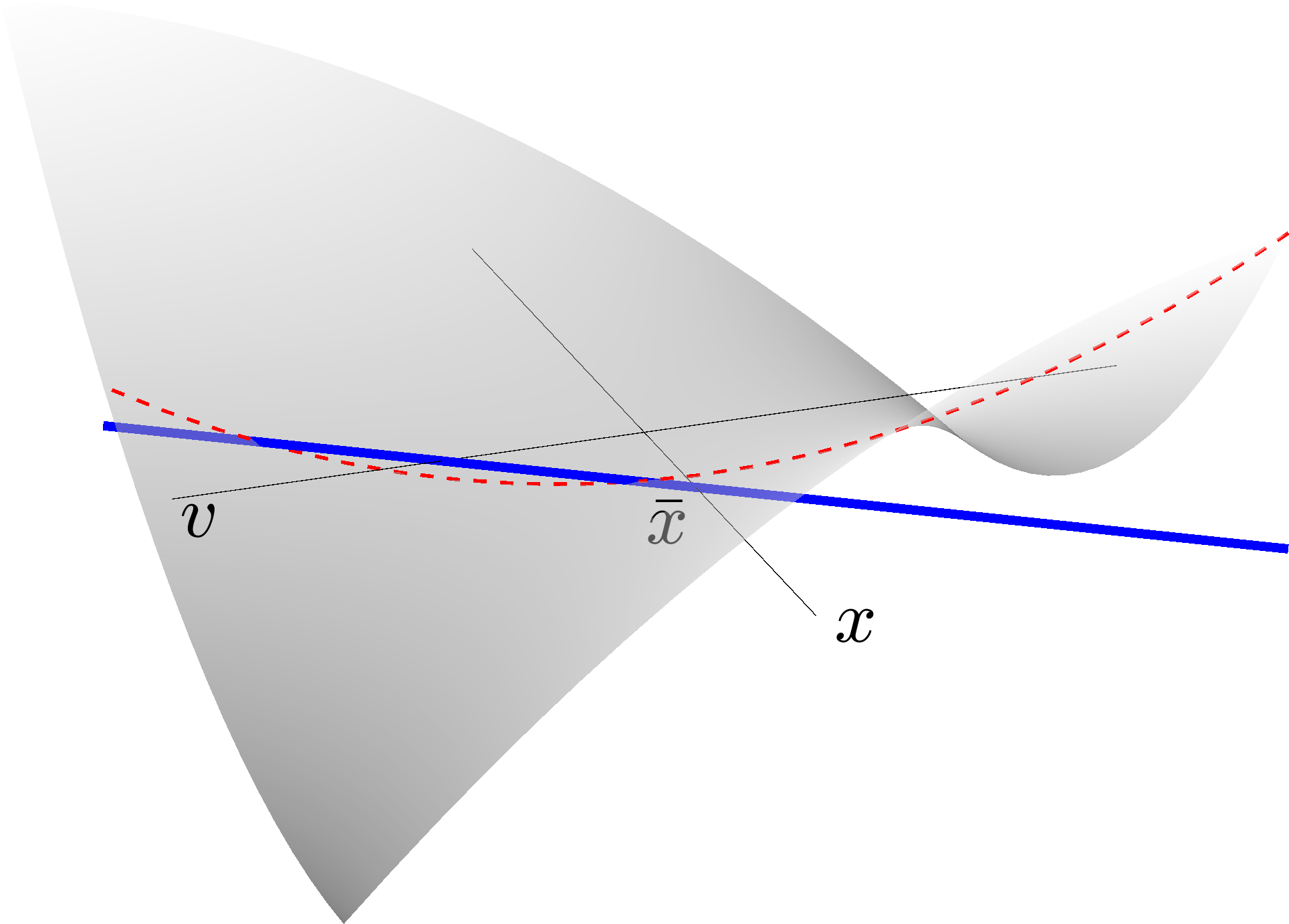
Figure 3: Depiction of a quadratic form on input-state pairs $(v,x)$. The blue line represents the linear-affine space of all input-state pairs satisfying the dynamics $\dot{x}=Ax+Bv$, $x(0)=\rm{\rm x}_{\rm i}$. When the input $v=0$, the state trajectory is the initial condition response $\bar{x}(t)=e^{At}\rm{\rm x}_{\rm i}$, depicted here as the intersection of the linear-affine space with the “$x$-axis”. The quadratic form ${\mbox{\large$\mathbf{q}$}}(x,v)$ over all signal pairs (not necessarily constrained by the dynamics) is depicted as the grey surface. $\mathbf{q}$ can have mixed signature as depicted here. The LQ Problem is to determine the infimum of the values of the quadratic form over the linear-affine constraint set (those values depicted here as the dashed red curve). Whether the infimum is finite or $-\infty$ depends on both the quadratic form and the system dynamics. In the case where the initial condition is zero (${\bar{x}}=0$), the constraint set is a subspace, and the constrained infimum can only be either $0$ or $-\infty$.

Theorem 12.

Consider a linear (possibly time-varying) system of the form

$$\dot{x}~{}=~{}Ax+Bv,\hskip 20.00003pt\hskip 20.00003ptt\in[0,{\scriptstyle T}],\hskip 20.00003ptx(0)={\rm x}_{\rm i},$$ (86)

and a quadratic form defined on $(x,v)$ pairs

$${\mbox{\large$\mathbf{q}$}}(x,w)~{}:=~{}\int_{0}^{{\scriptscriptstyle T}}\begin{bmatrix}x\\ v\end{bmatrix}^{*}\!\begin{bmatrix}Q&N\\ N^{*}&R\end{bmatrix}\begin{bmatrix}x\\ v\end{bmatrix}dt~{}=:\int_{0}^{{\scriptscriptstyle T}}\begin{bmatrix}x\\ v\end{bmatrix}^{*}\!{\begin{bmatrix}&&\\ &{\bm{Q}}&\\ &&\end{bmatrix}}\begin{bmatrix}x\\ v\end{bmatrix}dt~{}=:\int_{0}^{{\scriptscriptstyle T}}{\sf q}(x,v)~{}dt,$$

with $Q=Q^{*}$ and $R>0$. Consider also the Differential Linear Matrix Inequality (DLMI) over $[0,{\scriptstyle T}]$

$${\cal M}(\Lambda):={\bm{Q}}+\begin{bmatrix}{\dot{\Lambda}}+A^{*}\Lambda+\Lambda A&\Lambda B\\ B^{*}\Lambda&0\end{bmatrix}~{}\geq~{}0,\hskip 20.00003pt\Lambda({\scriptstyle T})=0.$$ (87)

1. The infimum of the quadratic form $\mathbf{q}$ subject to the constraints (86) is

   $$\inf~{}{\mbox{\large$\mathbf{q}$}}(x,w)~{}=~{}{\rm x}_{\rm i}^{*}~{}{\bar{\Lambda}}(0)~{}{\rm x}_{\rm i},$$ (88)

   where ${\bar{\Lambda}}$ is the maximal solution of the DLMI (87). This maximal solution satisfies the Differential Riccati Equation (DRE)

   $$Q+\dot{{\bar{\Lambda}}}+A^{*}{\bar{\Lambda}}+{\bar{\Lambda}}A-\left(N+{\bar{\Lambda}}B\right)R^{-1}\left(N+{\bar{\Lambda}}B\right)^{*}=0,\hskip 20.00003pt\hskip 20.00003pt{\bar{\Lambda}}({\scriptstyle T})=0.$$

2. If the solution of the DRE escapes to infinity within $[0,{\scriptstyle T}]$, then the infimum in (88) is $-\infty$. Otherwise, the optimal signal ${\bar{v}}$ is given by the state feedback

   $${\bar{v}}=R^{-1}(N^{*}+B^{*}{\bar{\Lambda}})~{}{\bar{x}},$$

Proof.

Since this is an infimization problem with fixed initial conditions, all the steps of the proof are essentially the same as the LQR case. The differences being that there are no assumptions on the definitness of $Q$, the additional term $N$ in ${\bm{Q}}$, and the interpretation of the joint covariance. We therefore only point out the differences in this proof.

The deterministic joint covariance of $x$ and $v$ is defined as

$$\Sigma(t)~{}:=~{}\begin{bmatrix}x(t)\\ v(t)\end{bmatrix}\begin{bmatrix}x^{*}(t)&v^{*}(t)\end{bmatrix}.$$

The primal and dual problems read exactly like the LQR case (66). The DLMI constraint of the dual in this case becomes

$$0~{}\leq~{}{\bm{Q}}+\begin{bmatrix}{\dot{\Lambda}}+A^{*}\Lambda+\Lambda A&\Lambda B\\ B^{*}\Lambda&0\end{bmatrix}=\begin{bmatrix}Q+{\dot{\Lambda}}+A^{*}\Lambda+\Lambda A&N+\Lambda B\\ (N+\Lambda B)^{*}&R\end{bmatrix},\hskip 20.00003pt\Lambda({\scriptstyle T})=0.$$ (89)

Finally, the dual problem is therefore

$$\sup_{{\cal M}(\Lambda)\geq 0,~{}\Lambda(T)=0}{\rm x}_{\rm i}^{*}\Lambda(0){\rm x}_{\rm i}$$ (90)

The solution of this last problem is obtained from the slightly more general Theorem 14 of Appendix A.5, which states that the maximal solution of the DLMI (89) is given by the solution of the DRE

$$Q+\dot{{\bar{\Lambda}}}+A^{*}{\bar{\Lambda}}+{\bar{\Lambda}}A-\left(N+{\bar{\Lambda}}B\right)R^{-1}\left(N+{\bar{\Lambda}}B\right)^{*}~{}=~{}0,\hskip 20.00003pt{\bar{\Lambda}}({\scriptstyle T})=0,$$

where the maximality property implies

$${\bar{\Lambda}}(t)~{}\geq~{}\Lambda(t)\hskip 20.00003pt\Rightarrow\hskip 20.00003pt{\rm x}_{\rm i}^{*}{\bar{\Lambda}}(0)~{}\!{\rm x}_{\rm i}~{}\geq~{}{\rm x}_{\rm i}^{*}\Lambda(0)~{}\!{\rm x}_{\rm i}\hskip 20.00003pt\Rightarrow\displaystyle\sup_{{\cal M}(\Lambda)\geq 0,~{}\Lambda(T)=0}{\rm x}_{\rm i}^{*}\Lambda(0)~{}\!{\rm x}_{\rm i}=~{}{\rm x}_{\rm i}^{*}{\bar{\Lambda}}(0)~{}\!{\rm x}_{\rm i}.$$

In this problem, the alignment condition (37) of conic duality reads

$$0~{} =~{}\left<{\bm{Q}}-({\mathcal{E}}^{*}-\mathcal{A}^{*}{\sf{\bm{I}}}_{\sf\bm{b}})(\bar{Y})\rule{0.0pt}{10.00002pt}\bm{,}{\bar{\Sigma}}\right>~{}=~{}\left<{\bm{Q}}+{\mathcal{E}}^{*}(\dot{{\bar{\Lambda}}})+\mathcal{A}^{*}({\bar{\Lambda}})\rule{0.0pt}{10.00002pt}\bm{,}{\bar{\Sigma}}\right>$$

$$=~{}\left<\begin{bmatrix}(N+{\bar{\Lambda}}B)R^{\text{-}\frac{1}{2}}\\ R^{\frac{1}{2}}\end{bmatrix}\begin{bmatrix}R^{\text{-}\frac{1}{2}}(N+{\bar{\Lambda}}B)^{*}&R^{\frac{1}{2}}\end{bmatrix}\bm{,}\begin{bmatrix}{\bar{x}}\\ {\bar{v}}\end{bmatrix}\begin{bmatrix}{\bar{x}}^{*}&{\bar{v}}^{*}\end{bmatrix}\right>,$$

where the last equality follows from the full-rank symmetric factorization (107) of ${\cal M}({\bar{\Lambda}}):={\bm{Q}}+{\mathcal{E}}^{*}(\dot{{\bar{\Lambda}}})+\mathcal{A}^{*}({\bar{\Lambda}})$ at the extremal ${\bar{\Lambda}}$. Lemma 3 implies that the product of the respective symmetric factors must be zero

$$0~{}=~{}\begin{bmatrix}R^{\text{-}\frac{1}{2}}(N+{\bar{\Lambda}}B)^{*}&R^{\frac{1}{2}}\rule{0.0pt}{10.00002pt}\end{bmatrix}\begin{bmatrix}{\bar{x}}\\ {\bar{v}}\end{bmatrix}\hskip 20.00003pt\Leftrightarrow\hskip 20.00003pt{\bar{v}}~{}=~{}-R^{\text{-}1}(N^{*}+B^{*}{\bar{\Lambda}})~{}{\bar{x}}.$$

Thus the optimal ${\bar{v}}$ is in the form of a state feedback. ∎

6.1 ${\sf L}^{2}(0,{\scriptstyle T})$-induced Norm, the Bounded-Real Lemma

Consider the (possibly time-varying) system with zero initial conditions

$$\dot{x}{} =~{}Ax~{}+~{}Bw,\hskip 20.00003ptt\in[0,{\scriptstyle T}],\hskip 20.00003ptx(0)={\rm x}_{\rm i}=0,$$ (91)

$$z{} =~{}Cx$$

This system has ${\sf L}^{2}[0,{\scriptstyle T}]$-induced norm less than $\gamma>0$ iff the IQC with quadratic form (3)

$${\mbox{\large$\mathbf{q}$}}(x,w)~{}:=~{}\scaleobj{.8}{\int_{{0}}^{{T}}}{\sf q}(x,w)dt~{}:=~{}\int_{0}^{T}\begin{bmatrix}x\\ w\end{bmatrix}^{*}\begin{bmatrix}\text{-}C^{*}C&0\\ 0&\gamma^{2}I\end{bmatrix}\begin{bmatrix}x\\ w\end{bmatrix}dt$$

is positive. Applying Theorem 12 we see that

$$\inf{\mbox{\large$\mathbf{q}$}}(x,w)~{}=~{}{\rm x}_{\rm i}\Lambda(0){\rm x}_{\rm i}~{}=~{}0$$

iff the DRE

$${\dot{\Lambda}}+A^{*}\Lambda+\Lambda A-\frac{1}{\gamma^{2}}\Lambda BB^{*}\Lambda-C^{*}C~{}=~{}0,\hskip 20.00003pt\Lambda(T)=0,$$

has a (bounded) solution over the interval $[0,{\scriptstyle T}]$. Otherwise the infimum is $-\infty$. The corresponding DLMI is given by

$${\bm{Q}}+\begin{bmatrix}{\dot{\Lambda}}+A^{*}\Lambda+\Lambda A&\Lambda B\\ B^{*}\Lambda&0\end{bmatrix}~{}=~{}\begin{bmatrix}{\dot{\Lambda}}+A^{*}\Lambda+\Lambda A-CC^{*}&\Lambda B\\ B^{*}\Lambda&\gamma^{2}I\end{bmatrix}~{}\geq~{}0,\hskip 20.00003pt\Lambda(T)=0.$$

Note that since in this problem the constant term in the DRE is $Q-NR^{\text{-}1}N^{*}=-C^{*}C\leq 0$, then by the monotonicity properties (Lemma LABEL:DRE_monotone.lemma) of the DRE, we have $\Lambda(t)\leq 0$. Furthermore, if $(C,A)$ is observable, then $\Lambda(t)<0$ for $t\in[0,{\scriptstyle T})$.

For future reference, if we assume the infinite-horizon version of this problem is arrived at by setting ${\dot{\Lambda}}=0$ in the above, then we have the statement

$$\|G\|_{2-{\rm i}}~{}\leq~{}\gamma\hskip 20.00003pt\Rightarrow\hskip 20.00003pt\exists\Lambda\leq 0,~{}\begin{bmatrix}A^{*}\Lambda+\Lambda A-CC^{*}&\Lambda B\\ B^{*}\Lambda&\gamma^{2}I\end{bmatrix}~{}\geq~{}0.$$

If we replace $\Lambda$ by $-X$, then the statement is equivalent to

$$\|G\|_{2-{\rm i}}~{}<~{}\gamma\hskip 20.00003pt\Rightarrow\hskip 20.00003pt\exists X\geq 0,~{}\begin{bmatrix}A^{*}X+XA+CC^{*}&XB\\ B^{*}X&-\gamma^{2}I\end{bmatrix}~{}\leq~{}0,$$

which is the more conventional statement of the Bounded Real Lemma. The reverse statement is easy to establish by a completion-of-squares argument. In addition, if $(C,A)$ is observable, then we can replace the condition $X\geq 0$ above with $X>0$. These arguments will be presented elsewhere for the infinite-horizon case.

6.2 Passivity over $(0,{\scriptstyle T})$, the Positive-Real Lemma

Appendix A.2 explains that the system

$$\dot{x}{} =~{}Ax~{}+~{}Bw,\hskip 20.00003ptt\in[0,{\scriptstyle T}],\hskip 20.00003ptx(0)={\rm x}_{\rm i}=0,$$ (91)

$$z{} =~{}Cx~{}+~{}Dw,$$

is passive over $[0,{\scriptstyle T}]$ iff the quadratic form (2)

$${\mbox{\large$\mathbf{q}$}}(x,w)~{}:=~{}\int_{0}^{T}\begin{bmatrix}x\\ w\end{bmatrix}^{*}\begin{bmatrix}0&C^{*}\\ C&D+D^{*}\end{bmatrix}\begin{bmatrix}x\\ w\end{bmatrix}dt$$

is positive. Theorem 12 states that

$$\inf{\mbox{\large$\mathbf{q}$}}(x,w)~{}=~{}{\rm x}_{\rm i}^{*}{\bar{\Lambda}}(0){\rm x}_{\rm i}~{}=~{}0$$

(i.e. the quadratic form constrained to the dynamics is positive) iff the the following DRE

$$0~{} =~{}{\dot{\Lambda}}+A^{*}\Lambda+\Lambda A-(C^{*}+\Lambda B)(D+D^{*})^{\text{-}1}(C+B^{*}\Lambda),\hskip 20.00003pt\Lambda({\scriptstyle T})=0,$$

has a (bounded) solution over the interval $[0,{\scriptstyle T}]$. Otherwise the infimum is $-\infty$. The associated DLMI is

$$\begin{bmatrix}{\dot{\Lambda}}+A^{*}\Lambda+\Lambda A&C^{*}+\Lambda B\\ C+B^{*}\Lambda&D+D^{*}\end{bmatrix},\hskip 20.00003pt\Lambda({\scriptstyle T})=0.$$

For this quadratic form, $N=C^{*}$, $Q=0$, and therefore $Q-NR^{\text{-}1}N^{*}=-C^{*}(D+D^{*})^{\text{-}1}C\leq 0$. The DRE definiteness Lemma LABEL:DRE_monotone.lemma states that the solution of the DRE is decreasing going backwards. Thus $\Lambda(t)\leq 0$ for $t\in[0,{\scriptstyle T}]$.

For future reference, if we assume the infinite-horizon version of this problem is arrived at by setting ${\dot{\Lambda}}=0$ in the above, then the infinite-horizon version of the problem is

$$G~{}\mbox{passive}\hskip 20.00003pt\Rightarrow\hskip 20.00003pt\exists\Lambda\leq 0,~{}\begin{bmatrix}A^{*}\Lambda+\Lambda A&C^{*}+PB\\ C+B^{*}P&D+D^{*}\end{bmatrix}~{}\geq~{}0.$$

In addition, if we again assume $(C,A)$ observable, then we can replace $\Lambda\leq 0$ above by $\Lambda<0$. If we define $P:=-\Lambda$, and multiply the LMI by a minus sign we get the statement

$$G~{}\mbox{passive}\hskip 20.00003pt\Leftrightarrow\hskip 20.00003pt\exists P\geq 0,~{}\begin{bmatrix}A^{*}P+PA&PB-C^{*}\\ B^{*}P-C&-D-D^{*}\end{bmatrix}~{}\leq~{}0,$$

which is the traditional statement of the “Positive Real Lemma”. Note the the converse implication follows from a standard “completing the squares” argument.

Appendix A Appendices

A.1 Trace Duality

Denote by $\sigma_{i}(A)$ the $i$’th singular value of a matrix $A$ when arranged in descending order. First note that for a square matrix $A$, we have that $\left|{\rm tr}\!\left(A\right)\right|\leq\sum_{i=1}^{n}\sigma_{i}(A)$. Indeed, let $A=U\Sigma V^{*}$ be the singular value decomposition of $A$, then

$$\left|{\rm tr}\!\left(A\right)\right|~{}=~{}\left|{\rm tr}\!\left(U\Sigma V^{*}\right)\right|~{}=~{}\left|{\rm tr}\!\left(\Sigma V^{*}U\right)\right|~{}=~{}\sum_{i=1}^{n}\sigma_{i}(A)~{}\left|\alpha_{i}\right|~{}\leq~{}\sum_{i=1}^{n}\sigma_{i}(A),$$

where $\left\{\alpha_{i}\right\}$ are the diagonal elements of $V^{*}U$ which are all such that $|\alpha_{i}|\leq 1$ since $V^{*}U$ is unitary.

Now let $M$ and $H$ be any two real matrices of the same dimensions

$${\rm tr}\!\left(H^{*}M\right)~{}\leq~{}\sum_{i=1}^{n}\sigma_{i}\big{(}H^{*}M\big{)}~{}\leq~{}\sum_{i=1}^{n}\sigma_{\max}(H)~{}\sigma_{i}\big{(}M\big{)}~{}=~{}\|H\|_{\infty}~{}\sum_{i=1}^{n}\sigma_{i}\big{(}M\big{)}~{}=~{}\|H\|_{\infty}\|M\|_{1}.$$

This inequality is tight in the sense that for any $H$

$$\sup_{\|M\|_{1}\leq 1}~{}{\rm tr}\!\left(H^{*}M\right)~{}=~{}\|H\|_{\infty}.$$

To prove this, let $H=U\Sigma V^{*}$ be a singular value decomposition

$${\rm tr}\!\left(H^{*}M\rule{0.0pt}{9.10004pt}\right)~{}=~{}{\rm tr}\!\left(V\Sigma U^{*}~{}M\rule{0.0pt}{9.10004pt}\right)~{}=~{}{\rm tr}\!\left(\Sigma~{}U^{*}\!MV\rule{0.0pt}{9.10004pt}\right),$$

Now choose $M$ such that $U^{*}MV={\sf diag}\!\left(1,0,\ldots,0\right)\rule{0.0pt}{10.00002pt}$. Since the $\|.\|_{1}$ norm is unitarily invariant, then $\|M\|_{1}=\|U^{*}MV\|_{1}=1$, and

$${\rm tr}\!\left(\Sigma~{}{\sf diag}\!\left(1,0,\ldots,0\right)\rule{0.0pt}{10.00002pt}\rule{0.0pt}{9.10004pt}\right)~{}=~{}\sigma_{\max}(H)~{}=~{}\|H\|_{\infty}.$$

A.2 ${{\sf H}^{\infty}}$ Norms and Passivity

Given a linear time-invariant system $G$, its ${{\sf H}^{\infty}}$ norm is the induced norm when the ${\sf L}^{2}$ norm on signals is used. It can also be characterized in the frequency domain by maximizing the singular values of the frequency response over all frequencies

$$\|G\|_{2-{\rm i}}~{}:=~{}\sup_{0\neq w\in{\sf L}^{2}}\frac{\|Gw\|_{{\sf L}^{2}}}{\|w\|_{{\sf L}^{2}}}~{}=~{}\|\hat{G}\|_{\infty}~{}:=~{}\sup_{\omega\in{\mathbb{R}}}~{}{\bar{\sigma}}\left(\rule{0.0pt}{10.00002pt}\hat{G}(j\omega)\right),$$

where $\hat{G}$ is the transfer function representing the system $G$. The frequency domain characterization only applies to time-invariant (and therefore infinite time horizon) systems. It is useful to have a time-domain criterion for the ${\sf L}^{2}$-induced norm of time-varying and/or finite-horizon systems. This means characterizing the ${\sf L}^{2}[0,{\scriptstyle T}]$-induced norm, which we now recast a a linear-quadratic optimization problem of the form (1).

Consider the state-space (possibly time-varying) system

$$\dot{x}{} =~{}Ax~{}+~{}Bw,\hskip 20.00003pt\hskip 20.00003ptt\in[0,{\scriptstyle T}],\hskip 20.00003ptx(0)=0,$$ (92)

$$z{} =~{}Cx~{}+~{}Dw,$$

and the following implications regarding its (finite or infinite-horizon) ${\sf L}^{2}$-induced norm

$$\begin{array}[]{rclrcl}\|G\|_{2-{\rm i}}~{}\leq~{}\gamma&\Longleftrightarrow&\displaystyle\sup_{0\neq w\in{\sf L}^{2}}\frac{\|z\|^{2}_{2}}{\|w\|^{2}_{2}}~{}\leq~{}\gamma^{2}&&\\ &\Updownarrow&&&\\ \forall~{}{w\in{\sf L}^{2}},~{}w\neq 0,&&\displaystyle\frac{\|z\|^{2}_{2}}{\|w\|^{2}_{2}}~{}\leq~{}\gamma^{2}&&\\ &\Updownarrow&&&\\ \forall~{}{w\in{\sf L}^{2}},&&\gamma^{2}\|w\|_{2}^{2}~{}\geq~{}\|z\|^{2}_{2}&&\\ &\Updownarrow&&&\\ \forall~{}{w\in{\sf L}^{2}},&&\gamma^{2}\|w\|_{2}^{2}-\|z\|^{2}_{2}~{}\geq~{}0&&\\ &\Updownarrow&&&\\ \displaystyle\inf_{w\in{\sf L}^{2}}&&\gamma^{2}\|w\|_{2}^{2}-\|z\|^{2}_{2}~{}=~{}0\hskip 100.00015pt\mbox{(since with $w=0$, $z=0$)}\end{array}$$

The above implications, though simple, are remarkable! They convert the problem of checking an induced norm inequality (a ratio of norms) to one of checking the positivity of a quadratic form over the input and output signals of a system. This problem fits in the general framework of (1) because the form is a quadratic form jointly on the input $w$ and the state $x$ (for notational simplicity, we set the direct-feedthrough term $D=0$ in the sequel)

$${\mbox{\large$\mathbf{q}$}}_{\mathrm{b}}~{} :=~{}\gamma^{2}\|w\|_{2}^{2}-\|z\|^{2}_{2}~{}=~{}\gamma^{2}\int_{0}^{T}w^{*}(t)w(t)~{}dt~{}-~{}\int_{0}^{T}z^{*}(t)z(t)~{}dt$$

$$=~{}\int_{0}^{T}\left(\gamma^{2}w^{*}w~{}-~{}x^{*}C^{*}Cx\rule{0.0pt}{10.00002pt}\right)~{}dt~{}=~{}\int_{0}^{T}\!\!\!\begin{bmatrix}x^{*}&w^{*}\end{bmatrix}\begin{bmatrix}\text{-}C^{*}C&0\\ 0&\gamma^{2}I\end{bmatrix}\begin{bmatrix}x\\ w\end{bmatrix}dt$$

$$=~{}\left<\begin{bmatrix}x\\ w\end{bmatrix}\bm{,}\begin{bmatrix}\text{-}C^{*}C&0\\ 0&\gamma^{2}I\end{bmatrix}\begin{bmatrix}x\\ w\end{bmatrix}\right>_{L^{2}[0,{\scriptstyle T}]}~{}=:~{}\left<\begin{bmatrix}x\\ w\end{bmatrix}\bm{,}{\bm{Q}}_{\mathrm{b}}\begin{bmatrix}x\\ w\end{bmatrix}\right>_{L^{2}[0,{\scriptstyle T}]},$$ (93)

where ${\bm{Q}}_{\mathrm{b}}$ is the (possibly time-varying) matrix function defined above. The subscript $\rm b$ references the bounded real lemma which is another name for the criterion of the same problem we are addressing.

Another important systems theory criterion is that of passivity.

Definition 13.

An ${\sf L}^{2}$-stable linear system $G$ is called passive over $(0,{\scriptstyle T})$ if all input output pairs $z=Gw$ with $w\in{\sf L}^{2}(0,{\scriptstyle T})$ (and zero initial conditions) satisfy

$$\left<z\bm{,}w\rule{0.0pt}{8.50006pt}\right>_{{\sf L}^{2}(0,{\scriptscriptstyle T})}~{}=~{}\scaleobj{.8}{\int_{{0}}^{{T}}}z^{*}(t)~{}w(t)~{}dt~{}\geq~{}0.$$ (94)

A system passive over $(0,\infty)$ is simply called passive.

We can again convert this to a question about the positivity of a quadratic form in input and state when the system $G$ is given by the realization (92)

$${\mbox{\large$\mathbf{q}$}}_{\rm p}~{} :=~{}\scaleobj{.8}{\int_{{0}}^{{T}}}z^{*}w~{}dt~{}=~{}\scaleobj{.8}{\int_{{0}}^{{T}}}(Cx+Dw)^{*}~{}w~{}dt~{}=~{}\scaleobj{.8}{\int_{{0}}^{{T}}}\left(x^{*}C^{*}w+w^{*}D^{*}w\rule{0.0pt}{10.00002pt}\right)~{}dt$$

$$=~{}\frac{1}{2}\int_{0}^{T}\begin{bmatrix}x^{*}&w^{*}\end{bmatrix}\begin{bmatrix}0&C^{*}\\ C&{D+D^{*}}\end{bmatrix}\begin{bmatrix}x\\ w\end{bmatrix}dt~{}=:~{}\frac{1}{2}\left<\begin{bmatrix}x\\ w\end{bmatrix}\bm{,}{\bm{Q}}_{\rm p}\begin{bmatrix}x\\ w\end{bmatrix}\right>_{{\sf L}^{2}(0,T)}.$$ (95)

Thus checking passivity of a system is equivalent to checking whether the quadratic form (95) is positive on all signals that satisfy the system’s equations.

A.3 Redundancy in Covariance Matrices

Let $z$ be a zero mean, continuous-time random process. Its instantaneous covariance matrix is defined as

$$\Sigma(t)~{}:=~{}{\mathbb{E}}\left[z(t)~{}z^{*}\!(t)\rule{0.0pt}{9.10004pt}\right],$$

which is a deterministic, matrix-valued function of $t$. Recall that covariance matrices are always positive $\Sigma(t)\geq 0$, and therefore have symmetric factorizations $\Sigma(t)=U(t)~{}U^{*}(t)$ for some other matrix $U(t)$. The dimensions of any such factorization has implications for dependencies between the components of the vector $z(t)$. This last statement will of course be only true up to second order statistics of the process $z$. For Gaussian processes, the statement is true without qualification.

In the following, the dependence on $t$ is suppressed for notational simplicity. Given a factorization ${\mathbb{E}}\left[z~{}z^{*}\rule{0.0pt}{9.10004pt}\right]=UU^{*}$, consider another random vector $\zeta:=Uw$, where $w$ is a zero-mean random vector with uncorrelated components (i.e. ${\mathbb{E}}\left[ww^{*}\right]=I$). With this construction, $\zeta$ and $z$ have the same second order statistics as can be easily verified

$${\mathbb{E}}\left[\zeta~{}\zeta^{*}\rule{0.0pt}{9.10004pt}\right]~{}=~{}{\mathbb{E}}\left[Uw~{}(Uw)^{*}\rule{0.0pt}{9.10004pt}\right]~{}=~{}{\mathbb{E}}\left[Uww^{*}U^{*}\rule{0.0pt}{9.10004pt}\right]~{}=~{}U~{}{\mathbb{E}}\left[ww^{*}\rule{0.0pt}{9.10004pt}\right]U^{*}~{}=~{}U~{}U^{*}~{}=~{}\Sigma.$$

Of course if $z$ and $w$ are Gaussian, then this means that $z$ and $\zeta$ have the same distribution.

We are interested in full-rank factorizations, i.e.

$$\Sigma~{}=~{}{\begin{bmatrix}\rule{0.0pt}{10.00002pt}\\ U\\ \rule{0.0pt}{10.00002pt}\end{bmatrix}}{\begin{bmatrix}~{}&U^{*}&~{}\end{bmatrix}},\hskip 20.00003pt\hskip 20.00003pt\Sigma\in{\mathbb{S}}_{n},~{}U\in{\mathbb{R}}^{n\times r},~{}r\leq n.$$

where $r={\rm\bf rk}\!\left(\Sigma\right)$, and therefore $U$ has full column rank. If $r<n$, then the original covariance matrix $\Sigma$ is not full rank. This indicates that there are redundancies in the description of the processes $z$ and $\zeta$. To see this, partition $\zeta$ and $U$ as follows

$$\zeta~{}=~{}\begin{bmatrix}\zeta_{1}\\ \zeta_{2}\end{bmatrix},\hskip 20.00003ptU~{}=~{}\begin{bmatrix}U_{1}\\ U_{2}\end{bmatrix},$$

so that $U_{1}$ is square (i.e. in ${\mathbb{R}}^{r\times r}$). Assume without loss of generality that $U_{1}$ is invertible. With this partition, the relation $\zeta=Uw$ now has the following implications

$$\begin{bmatrix}\zeta_{1}\\ \zeta_{2}\end{bmatrix}=\begin{bmatrix}U_{1}\\ U_{2}\end{bmatrix}w=\begin{bmatrix}U_{1}w\\ U_{2}w\end{bmatrix}\hskip 20.00003pt\Leftrightarrow\hskip 20.00003ptw=U_{1}^{-1}\zeta_{1}~{}~{}\mbox{and}~{}~{}\zeta_{2}=U_{2}w=U_{2}U_{1}^{-1}\zeta_{1}.$$ (96)

Thus $\zeta_{2}$ is a function of $\zeta_{1}$, or equivalently, the entire $\zeta$ vector is completely determined by its subcomponents $\zeta_{1}$, which is an $r$-vector. In an intuitive sense, the number of “degrees of freedom” in the random $n$-vector $\zeta$ is actually $r\leq n$, the rank of its covariance matrix.

Finally, if $z$ and $w$ are Gaussian, then the components of $z$ have the same joint distribution as the components of $\zeta$ as mentioned earlier. Since the components of $\zeta$ obey the relation (96), then the components of $z$ obey the same relation. The statements made above hold for each $t$, although the rank of the covariance matrix may depend on $t$.

A.4 Riccati Comparisons

Most of the arguments in this subsection are largely a reorganization of the classic arguments in [5] for the case of finite time horizon. The expression (97) below is from [5, Lemma 3]. The expression (98) is a slight modification which is needed when the matrix $M$ below has no specific definiteness.

1. Given the linear-quadratic portion of the Riccati opeator (i.e. without the constant term)

   $$\mathcal{R}_{\sf lq}(\Lambda)~{}:=~{}A^{*}\Lambda+\Lambda A-\Lambda M\Lambda,$$

   The difference $\mathcal{R}_{\sf lq}(\Lambda_{1})-\mathcal{R}_{\sf lq}(\Lambda_{2})$ can be expressed in several ways as follows

   $$\mathcal{R}_{\sf lq}(\Lambda_{1})-\mathcal{R}_{\sf lq}(\Lambda_{2})~{} =~{}A^{*}(\Lambda_{1}-\Lambda_{2})+(\Lambda_{1}-\Lambda_{2})A-\Lambda_{1}M\Lambda_{1}+\Lambda_{2}M\Lambda_{2}$$

   $$=~{}A^{*}(\Lambda_{1}-\Lambda_{2})+(\Lambda_{1}-\Lambda_{2})A-\Lambda_{1}M\Lambda_{1}+\Lambda_{2}M\Lambda_{2}$$

   $$\hskip 20.00003pt+\Lambda_{1}M\Lambda_{1}-\Lambda_{1}M\Lambda_{1}+\Lambda_{1}M\Lambda_{2}-\Lambda_{1}M\Lambda_{2}+\Lambda_{2}M\Lambda_{1}-\Lambda_{2}M\Lambda_{1}$$

   $$=~{}\left(A-M\Lambda_{1}\right)^{*}(\Lambda_{1}-\Lambda_{2})+(\Lambda_{1}-\Lambda_{2})\left(A-M\Lambda_{1}\right)+(\Lambda_{1}-\Lambda_{2})M(\Lambda_{1}-\Lambda_{2})$$ (97)

   $$=~{}\big{(}A+M(\Lambda_{1}+\Lambda_{2})/2\big{)}^{*}~{}(\Lambda_{1}-\Lambda_{2})~{}+~{}(\Lambda_{1}-\Lambda_{2})~{}\big{(}A+M(\Lambda_{1}+\Lambda_{2})/2)\big{)}$$ (98)

2. Consider solutions of two Riccati differential equations with different “$Q$-terms”

   $$0{} =~{}{\dot{\Lambda}}_{1}+A^{*}\Lambda_{1}+\Lambda_{1}A-\Lambda_{1}M\Lambda_{1}+Q_{1},\hskip 20.00003pt\Lambda_{1}({\scriptstyle T})=0,$$ (99)

   $$0{} =~{}{\dot{\Lambda}}_{2}+A^{*}\Lambda_{2}+\Lambda_{2}A-\Lambda_{2}M\Lambda_{2}+Q_{2},\hskip 20.00003pt\Lambda_{2}({\scriptstyle T})=0,$$

   with $Q_{1}\geq Q_{2}$. Define the difference ${\tilde{\Lambda}}:=\Lambda_{1}-\Lambda_{2}$, subtract the two equations and apply the Riccati difference formula (98) to obtain

   $$\dot{{\tilde{\Lambda}}}+\left(A+M\big{(}\Lambda_{1}+\Lambda_{2}\big{)}/2\right)^{*}{\tilde{\Lambda}}+{\tilde{\Lambda}}\left(A+M\big{(}\Lambda_{1}+\Lambda_{2}\big{)}/2\right)+\left(Q_{1}-Q_{2}\right)~{} =~{}0$$

   $$\Rightarrow\hskip 20.00003pt\dot{{\tilde{\Lambda}}}+\left(A+M\big{(}\Lambda_{1}+\Lambda_{2}\big{)}/2\right)^{*}{\tilde{\Lambda}}+{\tilde{\Lambda}}\left(A+M\big{(}\Lambda_{1}+\Lambda_{2}\big{)}/2\right)~{} =~{}-\left(Q_{1}-Q_{2}\right)~{}\leq~{}0.$$

   This is a differential Lyapunov inequality of the form (41) for ${\tilde{\Lambda}}$. Applying (45) we conclude that ${\tilde{\Lambda}}(t)\geq 0$, and for the differential Riccati equations with final conditions (99)

   $$Q_{1}(t)\geq Q_{2}(t),\hskip 10.00002ptt\in[0,{\scriptstyle T}]\hskip 20.00003pt\Rightarrow\hskip 20.00003pt\Lambda_{1}(t)\geq\Lambda_{2}(t),\hskip 10.00002ptt\in[0,{\scriptstyle T}]$$ (100)

3. Now consider the DRI (46) and the DRE obtained from it by setting the inequality to equality

   $$\left.\begin{aligned} \dot{\Lambda}+A^{*}\Lambda+\Lambda A-\Lambda~{}M~{}\Lambda+Q~{}\geq~{}0,\hskip 20.00003pt\Lambda({\scriptstyle T})=0,\\ \dot{{\bar{\Lambda}}}+A^{*}{\bar{\Lambda}}+{\bar{\Lambda}}A-{\bar{\Lambda}}~{}M~{}{\bar{\Lambda}}+Q~{}=~{}0,\hskip 20.00003pt{\bar{\Lambda}}({\scriptstyle T})=0.\end{aligned}\right\}\hskip 20.00003pt\Rightarrow\hskip 20.00003pt{\bar{\Lambda}}(t)\geq\Lambda(t),$$ (101)

   where the conclusion ${\bar{\Lambda}}(t)\geq\Lambda(t)$ follows from previous arguments. Indeed, the DRI is equivalent to the DRE (47) with the forcing function $H\geq 0$. A comparison of their “$Q$-terms” shows that $Q-(Q-H)=H\geq 0$, and therefore by the comparison result (100) ${\bar{\Lambda}}(t)\geq\Lambda(t)$ for all $t\in[0,{\scriptstyle T}]$, i.e. ${\bar{\Lambda}}$ is the maximal solution to the DRI.

A.5 DLMIs with initial or final conditions

Theorem 14 (Extremal Solutions).

Consider the linear matrix ${\cal M}$ and the associated Riccati $\mathcal{R}$ operators

$${\cal M}(\Lambda)~{} :=~{}{\bm{Q}}+{\mathcal{E}}^{{\bm{*}}}({\dot{\Lambda}})+\mathcal{A}^{{\bm{*}}}(\Lambda)~{}=\begin{bmatrix}Q+\dot{\Lambda}+A^{*}\Lambda+\Lambda A&N+\Lambda B\\ (N+\Lambda B)^{*}&R\end{bmatrix},$$ (102)

$$\mathcal{R}(\Lambda)~{} :=~{}{\dot{\Lambda}}+A^{*}\Lambda+\Lambda A-\left(N+\Lambda B\right)R^{\text{-}1}\left(N+\Lambda B\right)^{*}+Q,$$ (103)

where $R>0$ or $R<0$. Consider also initial- and final-value Differential Linear Matrix Inequalities (DLMIs) and their equivalent Differential Riccati Inequalities (DRIs) over $[t_{\rm i},t_{\rm f}]$

$$\left.\begin{array}[]{rclcrcl}{\cal M}(\Lambda)&\geq&0&\hskip 20.00003pt\Leftrightarrow&\hskip 20.00003pt\mathcal{R}(\Lambda)&\geq&0\\ \mbox{or}~{}{\cal M}(\Lambda)&\leq&0&\hskip 20.00003pt\Leftrightarrow&\hskip 20.00003pt\mathcal{R}(\Lambda)&\leq&0\end{array}\right\} \Lambda(t_{\rm i}) =\Lambda_{\rm i},\hskip 20.00003pt{\rm(DLMI_{i}/DRI_{i})}$$ (104)

$$\left.\begin{array}[]{rclcrcl}{\cal M}(\Lambda)&\geq&0&\hskip 20.00003pt\Leftrightarrow&\hskip 20.00003pt\mathcal{R}(\Lambda)&\geq&0\\ \mbox{or}~{}{\cal M}(\Lambda)&\leq&0&\hskip 20.00003pt\Leftrightarrow&\hskip 20.00003pt\mathcal{R}(\Lambda)&\leq&0\end{array}\right\} \Lambda(t_{\rm f}) =\Lambda_{\rm f}.\hskip 20.00003pt{\rm(DLMI_{f}/DRI_{f})}$$

Minimal and maximal solutions of the initial- and final-value inequalities respectively are given by the following Differential Riccati Equations (DREs)

$$\mathcal{R}({\underline{\Lambda}})~{} =~{}0, {\underline{\Lambda}}(t_{\rm i})=\Lambda_{\rm i},\hskip 20.00003pt{\rm(DRE_{i}):}~{}\mbox{\rm minimal-initial}$$ (105)

$$\mathcal{R}({\bar{\Lambda}})~{} =~{}0, {\bar{\Lambda}}(t_{\rm f})=\Lambda_{\rm f},\hskip 20.00003pt{\rm(DRE_{f}):}~{}\mbox{\rm maximal-final}$$ (106)

i.e. for any $\Lambda$ satisfying $\rm DLMI_{i}/DRI_{i}$ (resp. $\rm DLMI_{f}/DRI_{f}$)

$${\underline{\Lambda}}(t)~{}\leq~{}\Lambda(t)\hskip 20.00003pt\left(\rule{0.0pt}{10.00002pt}\mbox{resp.}~{}\Lambda(t)~{}\leq~{}{\bar{\Lambda}}(t)\right),\hskip 20.00003pt\hskip 20.00003ptt\in[t_{\rm i},t_{\rm f}].$$

Furthermore, at the extremal solutions, the matrix ${\cal M}$ has the full-rank symmetric factorization

$${\cal M}({\bar{\Lambda}})~{}=~{}\begin{bmatrix}(N+{\bar{\Lambda}}B)R^{\text{-}\frac{1}{2}}\\ R^{\frac{1}{2}}\end{bmatrix}\begin{bmatrix}R^{\text{-}\frac{1}{2}}(N+{\bar{\Lambda}}B)^{*}&R^{\frac{1}{2}}\end{bmatrix},$$ (107)

and similarly for ${\cal M}({\underline{\Lambda}})$.

Proof.

We consider the case ${\cal M}(\Lambda)\geq 0$ with $\Lambda(t_{\rm f})=\Lambda_{\rm f}$. The other three cases are argued similarly. The Riccati operator (103) can be written in the more standard form

$$\mathcal{R}(\Lambda)~{} :=~{}{\dot{\Lambda}}+A^{*}\Lambda+\Lambda A-\left(N+\Lambda B\right)R^{\text{-}1}\left(N+\Lambda B\right)^{*}+Q$$

$$=~{}{\dot{\Lambda}}+\big{(}A-BR^{\text{-}1}N^{*}\big{)}^{*}~{}\Lambda+\Lambda~{}\big{(}A-BR^{\text{-}1}N^{*}\big{)}-\Lambda~{}BR^{\text{-}1}B^{*}~{}\Lambda+\big{(}Q-NR^{\text{-}1}N^{*}\big{)}$$

$$=:~{}{\dot{\Lambda}}+\hat{A}^{*}\Lambda+\Lambda\hat{A}-\Lambda M\Lambda+\hat{Q}.$$ (108)

The Riccati comparison result (101) now implies that the solution ${\bar{\Lambda}}$ of $\mathcal{R}({\bar{\Lambda}})=0$ is maximal over all solutions of the $\rm DRE_{f}$, i.e. over all solutions of the $\rm DLMI_{f}$

For the factorization (55), note that the $\rm DRE_{f}$ for ${\bar{\Lambda}}$ implies

$$Q+\dot{{\bar{\Lambda}}}+A^{*}{\bar{\Lambda}}+{\bar{\Lambda}}A~{}=~{}(N+{\bar{\Lambda}}B)R^{\text{-}1}(N+{\bar{\Lambda}}B)^{*}.$$

Using this, the matrix ${\cal M}({\bar{\Lambda}})$ can be decomposed as

$$\begin{bmatrix}Q+\dot{{\bar{\Lambda}}}+A^{*}{\bar{\Lambda}}+{\bar{\Lambda}}A&(N+{\bar{\Lambda}}B)\\ (N+{\bar{\Lambda}}B)^{*}&R\end{bmatrix} =\begin{bmatrix}(N+{\bar{\Lambda}}B)R^{\text{-}1}(N+{\bar{\Lambda}}B)^{*}&N+{\bar{\Lambda}}B\\ (N+{\bar{\Lambda}}B)^{*}&R\end{bmatrix}$$

$$=\begin{bmatrix}(N+{\bar{\Lambda}}B)R^{\text{-}\frac{1}{2}}\\ R^{\frac{1}{2}}\end{bmatrix}\begin{bmatrix}R^{\text{-}\frac{1}{2}}(N+{\bar{\Lambda}}B)^{*}&R^{\frac{1}{2}}\end{bmatrix},$$

which is a full-rank factorization since $R$ (and therefore $R^{\frac{1}{2}}$) is assumed non-singular. ∎

References

• [1] R. E. Kalman, “Contributions to the theory of optimal control,” Bol. soc. mat. mexicana, vol. 5, no. 2, pp. 102–119, 1960.
• [2] V. Popov, “Hyperstability and optimality of automatic systems with several control functions,” Rev. Roum. Sci. Tech., Ser. Electrotech. Energ, vol. 9, no. 4, pp. 629–690, 1964.
• [3] R. E. Kalman, “Lyapunov functions for the problem of lur’e in automatic control,” Proceedings of the national academy of sciences, vol. 49, no. 2, pp. 201–205, 1963.
• [4] V. A. Yakubovich, “The solution of some matrix inequalities encountered in automatic control theory,” in Doklady Akademii Nauk, vol. 143, no. 6.   Russian Academy of Sciences, 1962, pp. 1304–1307.
• [5] J. Willems, “Least squares stationary optimal control and the algebraic riccati equation,” IEEE Transactions on automatic control, vol. 16, no. 6, pp. 621–634, 1971.
• [6] A. Megretski and A. Rantzer, “System analysis via integral quadratic constraints,” IEEE transactions on automatic control, vol. 42, no. 6, pp. 819–830, 1997.
• [7] S. Boyd, L. El Ghaoui, E. Feron, and V. Balakrishnan, Linear matrix inequalities in system and control theory.   SIAM, 1994.
• [8] S. P. Boyd and L. Vandenberghe, Convex optimization.   Cambridge university press, 2004.
• [9] C. Scherer and S. Weiland, “Linear matrix inequalities in control,” Lecture Notes, Dutch Institute for Systems and Control, Delft, The Netherlands, vol. 3, no. 2, 2000.
• [10] A. Gattami, “Generalized linear quadratic control,” IEEE Transactions on Automatic Control, vol. 55, no. 1, pp. 131–136, 2009.
• [11] ——, “Optimal decisions with limited information,” Ph.D. dissertation, Lund University, 2007.
• [12] S. You and A. Gattami, “H infinity analysis revisited,” arXiv preprint arXiv:1412.6160, 2014.
• [13] S. You, A. Gattami, and J. C. Doyle, “Primal robustness and semidefinite cones,” in 2015 54th IEEE Conference on Decision and Control (CDC).   IEEE, 2015, pp. 6227–6232.
• [14] A. Gattami and B. Bamieh, “Simple covariance approach to $H^{\infty}$ analysis,” IEEE Transactions on Automatic Control, vol. 61, no. 3, pp. 789–794, 2015.
• [15] A. Rantzer, “Linear quadratic dual control (cdc 2023 plenary presentation),” arXiv preprint arXiv:2312.06014, 2023.
• [16] M. A. Dahleh and J. Pearson, “$\ell^{1}$-optimal-feedback controllers for discrete-time systems,” in 1986 American Control Conference.   IEEE, 1986, pp. 1964–1968.
• [17] M. Dahleh and J. Pearson, “$L^{1}$-optimal compensators for continuous-time systems,” IEEE Transactions on Automatic Control, vol. 32, no. 10, pp. 889–895, 1987.
• [18] X. Qi, M. H. Khammash, and M. V. Salapaka, “A matlab package for multiobjective control synthesis,” in Proceedings of the 40th IEEE Conference on Decision and Control (Cat. No. 01CH37228), vol. 4.   IEEE, 2001, pp. 3991–3996.
• [19] M. V. Salapaka and M. Khammash, “Multi-objective mimo optimal control design without zero interpolation,” in Robustness in identification and control.   Springer, 1999, pp. 306–317.
• [20] L. Vandenberghe and S. Boyd, “Semidefinite programming,” SIAM review, vol. 38, no. 1, pp. 49–95, 1996.
• [21] R. Vinter, “Convex duality and nonlinear optimal control,” SIAM journal on control and optimization, vol. 31, no. 2, pp. 518–538, 1993.
• [22] A. Rantzer, “A dual to lyapunov’s stability theorem,” Systems & Control Letters, vol. 42, no. 3, pp. 161–168, 2001.
• [23] A. Mauroy, A. Sootla, and I. Mezić, “Koopman framework for global stability analysis,” The Koopman Operator in Systems and Control: Concepts, Methodologies, and Applications, pp. 35–58, 2020.
• [24] D. Angeli and E. D. Sontag, “Monotone control systems,” IEEE Transactions on automatic control, vol. 48, no. 10, pp. 1684–1698, 2003.
• [25] A. Rantzer and M. E. Valcher, “A tutorial on positive systems and large scale control,” in 2018 IEEE Conference on Decision and Control (CDC).   IEEE, 2018, pp. 3686–3697.
• [26] A. Rantzer, “Explicit solution to bellman equation for positive systems with linear cost,” in 2022 IEEE 61st Conference on Decision and Control (CDC).   IEEE, 2022, pp. 6154–6155.
• [27] B. Bamieh and M. Filo, “An input–output approach to structured stochastic uncertainty,” IEEE Transactions on Automatic Control, vol. 65, no. 12, pp. 5012–5027, 2020.
• [28] P. Seiler, “Stability analysis with dissipation inequalities and integral quadratic constraints,” IEEE Transactions on Automatic Control, vol. 60, no. 6, pp. 1704–1709, 2014.
• [29] A. Shapiro, “On duality theory of conic linear problems,” in Semi-infinite programming.   Springer, 2001, pp. 135–165.