Brickwall, Normal Modes and Emerging Thermality

Abstract

In this article, we demonstrate how black hole quasi-normal modes can emerge from a Dirichlet brickwall model normal modes. We consider a probe scalar field in a BTZ-geometry with a Dirichlet brickwall and demonstrate that as the wall approaches the event horizon, the corresponding poles in the retarded correlator become dense and yield an effective branch-cut. The associated discontinuity of the correlator carries the information of the black hole quasi-normal modes. We further demonstrate that a non-vanishing angular momentum non-perturbatively enhances the pole-condensing. We hypothesize that it is also related to quantum chaotic features of the corresponding spectral form factor, which has been observed earlier. Finally we discuss the underlying algebraic justification of this approximate thermalization in terms of the trace of the algebra.

I Introduction & Discussion

One of the earliest achievements of the AdS/CFT correspondence [1, 2, 3] had been to understand black holes in Anti-de Sitter spacetime in terms of distinguishing features of thermal correlators of a non-gravitational conformal field theory living on a codimension one surface that in turn can be identified as the boundary of that asymptotically AdS geometry. A precise holographic dictionary has been written in order for computing these correlators from the dual gravity set up and these computations have successfully gone through several qualitative and quantitative tests. Since in its weak form, the AdS/CFT correspondence relates a weakly coupled theory of gravity in presence of a black hole to a strongly coupled quantum field theory, such computations played pivotal roles to explore thermalization in strongly coupled quantum systems. A theoretical understanding of the latter, would otherwise be extremely difficult in absence of a perturbative scheme to compute these correlators directly.

In this work we aim to study a toy system of a (quantum) black hole by placing an appropriate boundary condition which caps off the geometry right before it reaches the horizon. Moreover, such a wall has the freedom to move infinitesimally close to the horizon. Clearly, this state should be represented by a pure state in the dual CFT, which, qualitatively, resembles a smooth fuzzball microstate in the supergravity approximation [4, 5]. The interesting question, from this perspective, would be to understand how a thermal physics emerges from such a system so that an asymptotic observer would never be able to distinguish it from an actual black hole. This pure state would then really be a good black hole mimicker. Furthermore, the AdS/CFT correspondence teaches us that the formation of horizon is a dual consequence of thermalization of the boundary CFT. Therefore, the afore-stated question boils down to asking, in a more general context, whether one could understand thermalization of a pure state in an isolated quantum system and the precision of detection thereof. This version, irrespective of whether the pure state can be associated with a fuzzball or not, lies at the heart of the black hole information paradox.

We compute the boundary Green’s function of an operator dual to a bulk probe scalar field with a Dirichlet boundary condition at a radial location outside the event horizon. We investigate whether this Green’s function encodes thermal behaviour in the limit where the Dirichlet hypersurface is located infinitesimally close to the event horizon. We will demonstrate and provide evidence that when the wall is placed at an $\epsilon$ distance away from the horizon, an asymptotic observer will observe an effective thermality and can read-off the associated well-known quasi-normal modes, from the normal modes. Here, $\epsilon$ is a dimensionless number measured in a suitable unit, e.g. the Planck length or the string length. This cut-off translates to a divergent IR time-scale: $\delta=\log\epsilon$ (see i.e. [12]), in the limit $\epsilon\to 0$. The quasi-normal modes (QNM) emerge from the inability to access this IR-divergent time-scale. In other words, given an arbitrarily long measurement time, one can always find an $\epsilon$ such that the information of the normal modes will repackage itself into yielding a set of QNM that coincides with the black hole QNM. Note that, our observations provide further and complementary evidence that a brickwall model can capture thermal features of a black hole as an effective description. Note that, recently in [13, 14] several aspects related to black hole thermodynamics have been evidenced in this model as well. Together and further emboldened by the observations in [4, 15, 16, 5], it strongly suggests that the brickwall model is, at least, a useful effective description of a quantum black hole.

The above statement is, largely, kinematical and holds for a linear spectrum in a two-dimensional black hole geometry [17]. Using our earlier results in [4, 15, 16, 5], we will further demonstrate that the IR-divergent time-scale is non-perturbatively further from $\delta$, once we include non-vanishing angular momenta along the compact direction. Curiously, this non-perturbative separation appears related to the appearance of quantum chaos, as discussed in the above works.

Our analyses provides a suggestive hint that resolving the Dirichlet wall from a classical event horizon is extremely difficult as the wall approaches the horizon. Note that the computation of the Green’s function is very different in the two cases, as the boundary condition on the wall should be different from the usual ingoing condition one typically employs at the black hole horizon. In the capped off geometry the natural choice is, as mentioned already, Dirichlet boundary conditions. This is similar to the brick wall model [18]. We find that the holographic correlator computed in this model contains a non-perturbative feature within a perturbative framework. The probe scalar and its subsequent quantization is simply a semi-classical perturbative analysis, as we move the Dirichlet wall infinitesimally close to the horizon. The dependence of thermality on this parameter is essentially the same as in [19]. The thermalization would be manifest through accumulations of poles of the retarded Green’s function on the real axis. Very close to the horizon, the poles become dense and effectively forms a continuum. In this limit, the continuum structure of the poles describes a branch cut up to a scale of resolution set by the infintesimal distance between the boundary wall and the black hole horizon. To resolve the branch-cut from a collection of dense poles one needs an incredibly large time-domain compared to the proper distance of the Dirichlet wall from the event horizon.

The rest of the paper is organized as follows. We will start with a lightning review on the computation of holographic Green’s function [20]. We will then move to our model of Dirichlet wall and use the same prescription to compute the boundary Green’s function, now with the Dirichlet condition on the wall instead. We will further discuss the analytic properties of the Green’s function to reveal the systematic approach to thermalization as mentioned above. Finally we will conclude with a discussion on how this approximate thermalization can be realized in terms of the classification of von Neumann algebra. In particular, we will demonstrate how the afore-mentioned limiting procedure captures an approximate transition from type I to type III von Neumann algebra.

II Scalar field in the brickwall

Let us begin with the non-rotating BTZ [21] geometry:

$$ds^{2}=-(r^{2}-r_{\rm H}^{2})dt^{2}+\frac{dr^{2}}{(r^{2}-r_{\rm H}^{2})}+r^{2}d\psi^{2}\,,$$ (1)

where $r=r_{\rm H}$ is the position of the horizon. Consider a probe scalar field of mass $\mu$ in this background that satisfies the Klein-Gordon equation:

$$\Box\Phi\equiv\frac{1}{\sqrt{|g|}}\partial_{\nu}\left(\sqrt{|g|}\partial^{\nu}\Phi\right)=\mu^{2}\Phi.$$ (2)

One can solve (2) analytically with the ansatz, $\Phi=\sum_{\omega,m}e^{-i\omega t}e^{im\psi}{\tilde{\phi}}(r)$. In terms of the redefined radial coordinate $z=1-{r_{\rm H}^{2}}/{r^{2}}$ with $z\in[0,1]$, we get two linearly independent solutions in terms of hypergeometric functions. The general solution is a linear combination:

$${\tilde{\phi}}\left(r(z)\right) \equiv\phi\left(z\right)=(1-z)^{\beta}\left[C_{1}\,z^{-i\alpha}{}_{2}F_{1}(a,b;c;z)\right.$$

$$\left.+\,C_{2}\,z^{i\alpha}\,{}_{2}F_{1}(1+a-c,1+b-c;2-c;z)\right]$$ (3)

where,

$$a=\beta-\frac{i}{2r_{\rm H}}(\omega+m),\ b=\beta-\frac{i}{2r_{\rm H}}(\omega-m),\ c=1-2i\alpha,$$

$$\text{with}\ \ \ \alpha=\frac{\omega}{2r_{\rm H}},\ \ \beta=\frac{1}{2}(1-\sqrt{1+\mu^{2}}).$$ (4)

We now impose a Dirichlet wall at a radial position $z=z_{0}$, slightly above the event horizon at $z=0$[4, 15, 5]. We demand $\phi(z=z_{0})=0$, instead of the ingoing boundary condition on the horizon. This boundary condition fixes the ratio of the undetermined constants $C_{1}$ and $C_{2}$ of the general solution as

$$R_{C_{2}C_{1}}=\frac{C_{2}}{C_{1}}=-z_{0}^{-2i\alpha}\frac{{}_{2}F_{1}(a,b;c;z_{0})}{{}_{2}F_{1}(1+a-c,1+b-c;2-c;z_{0})}.$$ (5)

Following the prescription of [20], and using the above result, we expand the solution near the boundary at $z=1$

$$\phi(z)_{bdry}\sim R_{1}(1-z)^{\frac{1}{2}(1-\sqrt{1+\mu^{2}})}+R_{2}(1-z)^{\frac{1}{2}(1+\sqrt{1+\mu^{2}})},$$ (6)

where

$$R_{1} =\frac{\Gamma(c)\Gamma(c-a-b)}{\Gamma(c-a)\Gamma(c-b)}+R_{C_{2}C_{1}}\frac{\Gamma(2-c)\Gamma(c-a-b)}{\Gamma(1-a)\Gamma(1-b)}$$ (7)

$$R_{2} =\frac{\Gamma(c)\Gamma(a+b-c)}{\Gamma(a)\Gamma(b)}+R_{C_{2}C_{1}}\frac{\Gamma(2-c)\Gamma(a+b-c)}{\Gamma(1+a-c)\Gamma(1+b-c)}$$ (8)

Identifying $R_{2}$ and $R_{1}$ as the normalizable and the non-normalizable modes respectively, the boundary Green’s function can be computed by taking their ratio

$$G(\omega,m)=\frac{R_{2}}{R_{1}}=\frac{\frac{\Gamma(c)\Gamma(a+b-c)}{\Gamma(a)\Gamma(b)}+R_{C_{2}C_{1}}\frac{\Gamma(2-c)\Gamma(a+b-c)}{\Gamma(1+a-c)\Gamma(1+b-c)}}{\frac{\Gamma(c)\Gamma(c-a-b)}{\Gamma(c-a)\Gamma(c-b)}+R_{C_{2}C_{1}}\frac{\Gamma(2-c)\Gamma(c-a-b)}{\Gamma(1-a)\Gamma(1-b)}},$$ (9)

with $R_{C_{2}C_{1}}$ given in (5).

The Green’s function (9) possesses a very rich pole structure and the dynamics thereof, as we move the wall close to the horizon of the black hole. As shown in figure 1, for a fixed value of $m$, the poles tend to accumulate when the wall is moved closer to the horizon. A very similar dynamics of the poles can also be obtained by keeping $n$ fixed instead of $m$. In what follows, we will investigate this phenomenon of pole accumulation more closely, towards obtaining a physical interpretation of the same.

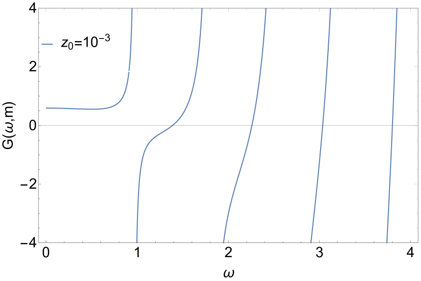
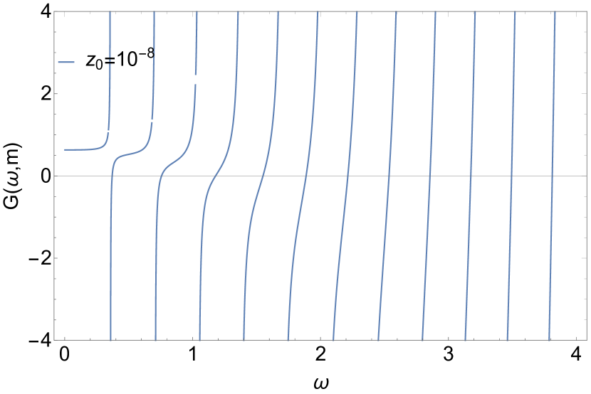
Figure 1: Pole Structure of $G_{\omega}(n,m)$ for fixed $m=1$. Poles are coming closer and closer as we move the position of the stretched horizon towards the event horizon. $\mu=1$ here for the both figures.

II.1 Analytic properties of the Green’s function

The Green’s function (9) has poles when the denominator vanishes, namely when

$$\frac{\Gamma(c)}{\Gamma(c-a)\Gamma(c-b)}+R_{C_{2}C_{1}}\frac{\Gamma(2-c)}{\Gamma(1-a)\Gamma(1-b)}=0$$ (10)

Note, solutions of (10) are the normal modes for the probe scalar[4, 5]. This is clearly different from the QNM which is obtained by imposing ingoing boundary condition.

When the wall is infinitesimally close to the event horizon, then, from (5), $R_{C_{1}C_{2}}\approx-z_{0}^{-2i\alpha}$. Accordingly, (10) can be written as:

$$\alpha\log z_{0}+\text{Arg}\left[\frac{\Gamma(c)}{\Gamma(c-a)\Gamma(c-b)}\right]=n\pi,\hskip 2.84544pt\text{with}\hskip 2.84544ptn\in\mathbf{Z}.$$ (11)

Solution to (11) provides quantized values of frequency $\omega=\omega_{n,m}$ as the normal mode frequencies. The poles of the Green’s function located at these quantised values of frequency gets denser as the wall moves closer to the black hole horizon at $z=0$. We already observed this in Figure 1, for a fixed value of $m$.

In order to get an intuition of how fast that density of poles increases, we can simply fix a cutoff in frequency at $\omega=\omega_{max}$ and count the number of poles as a function of the distance between the wall of the box and the black hole horizon. This estimate can be done both for fixed $m$ or $n$. The results are demonstrated in Figure 2.

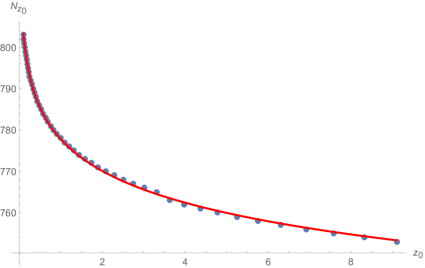
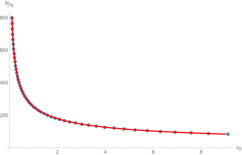
Figure 2: $N_{z_{0}}$ vs. $z_{0}$ for fixed $m$ (left) and fixed $n$ (right) respectively. $\mu=0$ here. The horizontal axis is scaled up by a factor of $10^{31}$ for better visualization. The numerical data are fitted with appropriate fitting functions which are discussed in the main text.

To better visualize, We have fitted the numerical data with appropriate functions. For example, when $m$ is held fixed, the fitting function is:

$$a+b\log(1/z_{0})\ ,$$ (12)

where $\{a,b\}$ are the fitting parameters. This is guessed from e.g. the s-wave answer of [5, 17]. As mentioned earlier, the branch-cut approximation will break down at an IR-divergent time-scale $\delta=|\log(z_{0})|$. On the other hand, when $n$ is fixed, the fitting function is:

$$a+bz_{0}^{-1/2}\ ,$$ (13)

and therefore the corresponding IR-divergent time-scale, $e^{c\delta}$ with an order one number $c$, where the branch-cut approximation breaks down is exponentially larger. Note that, this fitting function is inspired from analytic WKB-approximations discussed in [5]. It is possible to obtain an analytic expression of how dense these poles are along $m$-direction. This result is given by product-log functions and the precise expression involves nested logarithms and powers of them. The existence of the hierarchy is therefore warranted[22].

It is clear from the that the rate of accumulation of poles along $m$-direction is much larger compared to when we fix $m$ to a particular value. Combined with earlier work in [4, 5], where it was pointed out a quantum chaotic feature emerged from level-repulsion along the $m$-direction, the greater accumulation rate along this direction further supports the emerging thermal picture due to the spectral correlations along this direction. It appears to be a rather important qualifier in this framework, where pole accumulation happens along both directions, but level-repulsion occurs in one of them. This will be a very interesting point to understand better.

II.2 From discrete poles to a branch-cut: approaching thermality

As we discussed in the preceding section, the poles of Green’s function accumulate systematically as we move the wall at $z=z_{0}$ towards the horizon at $z=0$. At a sufficiently small value of $z=z_{0}$, as $z_{0}\rightarrow 0$, the poles form a continuous branch-cut for a low energy asymptotic observer. As we just argued, however, this statement is non-perturbatively enhanced in the presence of a non-vanishing angular momenta. We will now demonstrate that this branch-cut approximation encodes the black hole QNM data.

Now we are in a position to make heavy but straightforward use of [19]. The detailed analyses are essentially identical to [19] and therefore instead of writing them out, we point out the key steps.

Let us, for simplicity, fix $m$ to a particular value $m=m_{0}$ for which we denote the normal mode frequencies as $\omega_{n,m_{0}}\equiv\omega_{n}$. In this case, the Green’s function at fixed $z_{0}$ can be written in the form of [19]

$$G(\omega,m_{0})=\sum_{n}\left(\frac{\omega}{\omega_{n}}\right)^{\Delta}\frac{\text{Res}(G,\omega_{n})}{\omega-\omega_{n}},$$ (14)

where ${\text{Res}}(G,\omega_{n})$ is the residue of the Green’s function at $\omega=\omega_{n}$. Here the factor $\omega^{\Delta}$ is introduced to ensure that the function $\frac{G(\omega,m_{0})}{\omega^{\Delta}}$ falls off and eventually vanishes at the boundary of the contour at $\omega\rightarrow\infty$. When the poles at $\omega=\omega_{n}$ come infinitesimally close to each other making the structure sufficiently dense, one can instead consider, as a good approximation, a continuum distribution of poles, simply by replacing the sum over $n$ with an integral over frequency:

$$G(\omega,m_{0})\approx\int d\omega_{n}\frac{\rho_{\omega}(\omega_{n},m_{0})}{\omega-\omega_{n}},$$ (15)

where

$$\rho_{\omega}(\omega_{n},m_{0})=\left(\frac{\omega}{\omega_{n}}\right)^{\Delta}{\text{Res}}(G,\omega_{n})\frac{dn}{d\omega_{n}}.$$ (16)

From (15), it is straightforward to show

$$G(\omega+i\epsilon,m_{0})-G(\omega-i\epsilon,m_{0}) =2i\,{\rm{Im}}G_{\cal R}(\omega,m_{0})$$

$$=2\pi i\rho_{\omega}(\omega,m_{0}),$$ (17)

where $G_{\cal R}(\omega,m_{0})$ is the retarded Green’s function. This shows that, indeed, as the poles become sufficiently dense, the correlator effectively develops a branch cut with the discontinuity given by the function $\rho_{\omega}(\omega,m_{0})$.

The branch-cut discontinuity $\rho_{\omega}(\omega,m_{0})$ for our Green’s function (9) which can be re-expressed in the form:

$$G(\omega,m)=\frac{G_{\text{bh}}(\omega)+R_{C_{2}C_{1}}\frac{\Gamma(2-c)\Gamma(a+b-c)}{\Gamma(1+a-c)\Gamma(1+b-c)}\frac{\Gamma(c-a)\Gamma(c-b)}{\Gamma(c)\Gamma(c-a-b)}}{1+R_{C_{2}C_{1}}\frac{\Gamma(2-c)}{\Gamma(1-a)\Gamma(1-b)}\frac{\Gamma(c-a)\Gamma(c-b)}{\Gamma(c)}},$$ (18)

where $G_{\text{bh}}$ is the retarded Green’s function of the BTZ black hole.

Using the above results, it is now straightforward to show that

$$2\pi\rho_{\omega}(\omega,m_{0})={\rm{Im}}\,G_{\cal R}(\omega,m_{0})=-\text{Im}\,G_{\text{bh}}(\omega,m_{0}),$$ (19)

which states that in the limit when the wall is sufficiently close to the horizon of the black hole, the imaginary part of the scalar Green’s function is indistinguishable from that of the thermal Green’s function of the black hole for a sufficiently low energy asymptotic observer and hence contains the black hole quasi-normal modes. This is qualitatively similar to the information paradox[23, 24, 25, 6, 9]. The energy scale of the observer should be much lower than the scale set by the distance between the wall and the event horizon.

A complementary approach to understand this approximate thermality was adopted in [14] where the same cutoff scale was obtained by comparing the microcanonical entropy of the horizonless configuration to that associated with a Hartle-Hawking state. This approach is quite similar in spirit to that in [26].

The equation (19) automatically ensures the matching of the effective temperature in the aforementioned limit to that of a BTZ black hole. This can be confirmed by explicitly calculating the position space representation of the Green’s function as well. This provides an even stronger conclusion that when the wall is infinitesimally close to the event horizon, at the leading order, the position space Green’s function becomes indistinguishable from the corresponding thermal correlation function. This ensures, as claimed above, the matching of the effective temperature of the box to that of the black hole.

While this matching is already surprising, one might still wonder about the fact that Green’s function (9) has real poles in the form of the normal modes, while a black hole is characterized by complex QNM poles. Nonetheless, in the pole accumulation to the branch-cut limit, the corresponding jump function across the branch cut becomes the black hole Green’s function, as evident from (II.2) and (19), and therefore contains the complex QNM poles of the black hole.

III Algebra and factorization

The emergence of the approximate thermality in the limit $z_{0}\to 0$ carries an underlying algebraic justification. When the cut-off is placed at a finite $z_{0}$, the algebra of observables, $\mathcal{A}$ is of type I_∞. Correspondingly, there exists the natural notion of a trace functional as we are used to from quantum mechanics[27, 28, 29]. In the limit $z_{0}\to 0$, the algebra type transforms to type III [17]. To verify this explicitly, we need to ensure that, in the limit $z_{0}\to 0$, there is no tracial state $\omega_{\tr}$ on the algebra, i.e. there is no state satisfying

$$\omega_{\tr}(ab)=\omega_{\tr}(ba)\quad\text{for any}\quad a,b\in\mathcal{A}\,.$$ (20)

This can be established as follows. Given a finite value of $z_{0}$, solution of the scalar wave equation yields a set of quantized simple harmonic oscillator data $\{a_{r,\omega_{n,m}},\omega_{n,m}\}$. Furthermore, we showed that in the limit $z_{0}\to 0$, an effective thermal description emerges at an inverse temperature $\beta=\frac{2\pi l^{2}}{r_{h}}$. The associated state vector is given by[17]

$$|\beta\rangle_{\epsilon}=\bigotimes_{\omega_{n}}\sqrt{1-e^{-\beta\omega_{n}}}e^{-\beta\frac{\omega_{n}}{2}a_{l,\omega_{n}}^{\dagger}a_{r,\omega_{n}}^{\dagger}}|0_{l,\omega_{n}},0_{r,\omega_{n}}\rangle\,.$$ (21)

From the perspective of the state, this expression can be thought of as an approximation of the topped-up Boulware vacuum as a Hartle-Hawking state. Such an approximation was argued back in [30] and was recently revisited through a comparison of the Wightman function in the aforementioned limit in [14]. This identification is a key to the factorization map discussed in [26]. The cutoff scale provides an energy topping on the conventional Boulware vacuum, which in the context of dual CFT should have an interpretation of a defect operator. We will elaborate this interesting connection in a future publication [22].

Using the vector (21), we evaluate the thermal expectation value of $a_{r,\omega_{n}}(t)a_{r,\omega_{n}}^{\dagger}(0)$ as well as $a_{r,\omega_{n}}^{\dagger}(0)a_{r,\omega_{n}}(t)$ and find that the two expressions differ for arbitrary $\delta$. This eventually allows us to diagnose that there is no tracial state in the limit $z_{0}\to 0$. In particular we find

$$G(t)=F(t-i\beta)\,,$$ (22)

where,

$$G(t) =\langle a_{r,\omega_{n,m}}(t)a_{r,\omega_{n,m}}^{\dagger}(0)\rangle_{\beta,z_{0}}$$

$$F(t) =\langle a_{r,\omega_{n,m}}^{\dagger}(0)a_{r,\omega_{n,m}}(t)\rangle_{\beta,z_{0}}\,.$$ (23)

This is the KMS condition, which, in terms of the corresponding Fourier modes $f(\omega)$ and $g(\omega)$ of the functions $F(t)$ and $G(t)$ respectively, translates to

$$g(\omega)=e^{-\beta\omega_{n,m}}f(\omega)\,.$$ (24)

The relative scaling with the exponential tells that the two functions are not generally equal. Therefore, $F\neq G$ and their difference is non-zero. It can be easily verified that

$$\left.e^{-\beta\omega_{n,m}}\right|_{m={\rm const}}\sim e^{\frac{\#}{|\ln{z_{0}}|}}\ ,\left.e^{-\beta\omega_{n,m}}\right|_{n={\rm const}}\sim e^{\#z_{0}^{1/2}}\ .$$ (25)

We have explicitly used (12) and (13) in deriving the above and $\#$ denotes an order one number that does not play any role in the conclusions. Now comes the main catch point which will justify the role of the emergent IR time scale mentioned before. In the limit of $z_{0}\to 0$, both the exponential factors tends to 1 and this happens independent of the number $\#$ and for any finite temperature. This implies so long as we can resolve the respective time-scales, the algebra remains to be of type I. However, when we are no longer able to do that, and the spectrum effectively becomes a continuum with $e^{-\beta\omega_{n,m}}\rightarrow e^{-\beta\omega}$, one can no longer define a tracial state for any finite $\beta$. Accordingly, the algebra type changes to type III.

This emphasizes further the importance of the continuum spectrum approximation in our analysis. Although both the exponential factors in (25) have the same limiting behaviour in the limit $z_{0}\to 0$, the gradient of the exponents along $n$ and $m$ directions differ and they determine to what extent this continuous approximation for the spectrum is valid. A faster gradient in the $m$ direction potentially explain the appearance of ramp in the spectral form factor for fixed values of $n$ as observed in [4].

This is an explicit example where the rate of approach of a type I von Neumann algebra to a type III algebra is related to the existence of quantum chaotic structures.

In [31] it was argued that geometric phases associated to the entanglement pattern can be used to distinguish between different algebra types. The trace on any type of algebra is defined by a state vector with vanishing geometric phases, corresponding to maximal entanglement. Therefore, as type III algebras do not have a trace, any state vector for such algebras has geometric phases. It would be interesting to determine whether this can be made quantitatively precise in the current setting, i.e. how the limit $z_{0}\to 0$ affects these geometric phases, in particular their values hinting at an approximate algebraic transition. A detailed exploration of this will appear in [22].

References

- Maldacena [1998] J. M. Maldacena, The Large N limit of superconformal field theories and supergravity, Adv. Theor. Math. Phys. 2, 231 (1998), arXiv:hep-th/9711200 .
- Witten [1998] E. Witten, Anti-de Sitter space and holography, Adv. Theor. Math. Phys. 2, 253 (1998), arXiv:hep-th/9802150 .
- Gubser et al. [1998] S. S. Gubser, I. R. Klebanov, and A. M. Polyakov, Gauge theory correlators from noncritical string theory, Phys. Lett. B 428, 105 (1998), arXiv:hep-th/9802109 .
- Das et al. [2023a] S. Das, C. Krishnan, A. P. Kumar, and A. Kundu, Synthetic fuzzballs: a linear ramp from black hole normal modes, JHEP 01, 153, arXiv:2208.14744 [hep-th] .
- Das and Kundu [2023] S. Das and A. Kundu, Brickwall in Rotating BTZ: A Dip-Ramp-Plateau Story, (2023), arXiv:2310.06438 [hep-th] .
- Mathur [2005] S. D. Mathur, The Fuzzball proposal for black holes: An Elementary review, Fortsch. Phys. 53, 793 (2005), arXiv:hep-th/0502050 .
- Susskind et al. [1993] L. Susskind, L. Thorlacius, and J. Uglum, The Stretched horizon and black hole complementarity, Phys. Rev. D 48, 3743 (1993), arXiv:hep-th/9306069 .
- Almheiri et al. [2013] A. Almheiri, D. Marolf, J. Polchinski, and J. Sully, Black Holes: Complementarity or Firewalls?, JHEP 02, 062, arXiv:1207.3123 [hep-th] .
- Lunin and Mathur [2002] O. Lunin and S. D. Mathur, AdS / CFT duality and the black hole information paradox, Nucl. Phys. B 623, 342 (2002), arXiv:hep-th/0109154 .
- Kanitscheider et al. [2007] I. Kanitscheider, K. Skenderis, and M. Taylor, Fuzzballs with internal excitations, JHEP 06, 056, arXiv:0704.0690 [hep-th] .
- Bena et al. [2015] I. Bena, S. Giusto, R. Russo, M. Shigemori, and N. P. Warner, Habemus Superstratum! A constructive proof of the existence of superstrata, JHEP 05, 110, arXiv:1503.01463 [hep-th] .
- Alam et al. [2012] M. S. Alam, V. S. Kaplunovsky, and A. Kundu, Chiral Symmetry Breaking and External Fields in the Kuperstein-Sonnenschein Model, JHEP 04, 111, arXiv:1202.3488 [hep-th] .
- Krishnan and Pathak [2023] C. Krishnan and P. S. Pathak, Normal Modes of the Stretched Horizon: A Bulk Mechanism for Black Hole Microstate Level Spacing, (2023), arXiv:2312.14109 [hep-th] .
- Burman et al. [2023] V. Burman, S. Das, and C. Krishnan, A Smooth Horizon without a Smooth Horizon, (2023), arXiv:2312.14108 [hep-th] .
- Das et al. [2023b] S. Das, S. K. Garg, C. Krishnan, and A. Kundu, Fuzzballs and random matrices, JHEP 10, 031, arXiv:2301.11780 [hep-th] .
- Das et al. [2023c] S. Das, S. K. Garg, C. Krishnan, and A. Kundu, What is the Simplest Linear Ramp?, (2023c), arXiv:2308.11704 [hep-th] .
- Soni [2023] R. M. Soni, A Type Approximation of the Crossed Product, (2023), arXiv:2307.12481 [hep-th] .
- ’t Hooft [1985] G. ’t Hooft, On the Quantum Structure of a Black Hole, Nucl. Phys. B 256, 727 (1985).
- Giusto et al. [2023] S. Giusto, C. Iossa, and R. Russo, The black hole behind the cut, JHEP 10, 050, arXiv:2306.15305 [hep-th] .
- Son and Starinets [2002] D. T. Son and A. O. Starinets, Minkowski space correlators in AdS / CFT correspondence: Recipe and applications, JHEP 09, 042, arXiv:hep-th/0205051 .
- Banados et al. [1992] M. Banados, C. Teitelboim, and J. Zanelli, The Black hole in three-dimensional space-time, Phys. Rev. Lett. 69, 1849 (1992), arXiv:hep-th/9204099 .
- [22] S. Banerjee, S. Das, M. Dorband, and A. Kundu, To Appear, To Appear .
- Page [1993] D. N. Page, Information in black hole radiation, Phys. Rev. Lett. 71, 3743 (1993), arXiv:hep-th/9306083 .
- Maldacena [2003] J. M. Maldacena, Eternal black holes in anti-de Sitter, JHEP 04, 021, arXiv:hep-th/0106112 .
- Mathur [2009] S. D. Mathur, The Information paradox: A Pedagogical introduction, Class. Quant. Grav. 26, 224001 (2009), arXiv:0909.1038 [hep-th] .
- Jafferis and Kolchmeyer [2019] D. L. Jafferis and D. K. Kolchmeyer, Entanglement Entropy in Jackiw-Teitelboim Gravity, (2019), arXiv:1911.10663 [hep-th] .
- Witten [2021] E. Witten, Why Does Quantum Field Theory In Curved Spacetime Make Sense? And What Happens To The Algebra of Observables In The Thermodynamic Limit?, (2021), arXiv:2112.11614 [hep-th] .
- Witten [2022] E. Witten, Gravity and the crossed product, JHEP 10, 008, arXiv:2112.12828 [hep-th] .
- Witten [2023] E. Witten, Algebras, Regions, and Observers, (2023), arXiv:2303.02837 [hep-th] .
- Mukohyama and Israel [1998] S. Mukohyama and W. Israel, Black holes, brick walls and the Boulware state, Phys. Rev. D 58, 104005 (1998), arXiv:gr-qc/9806012 .
- Banerjee et al. [2023] S. Banerjee, M. Dorband, J. Erdmenger, and A.-L. Weigel, Geometric phases characterise operator algebras and missing information, JHEP 10, 026, arXiv:2306.00055 [hep-th] .