High-energy QCD dynamics from bottom
flavor fragmentation at the Hi-Lumi LHC

Abstract

We study the inclusive production of hadrons with bottom flavor at the LHC and its luminosity upgrade. We describe the collinear fragmentation of singly $b$-flavored hadrons, $B$ mesons and $\Lambda_{b}$ baryons, via the KKSS07 determination of fragmentation functions, while for charmed $B$ mesons, $B_{c}(^{1}S_{0})$ and $B_{c}(^{3}S_{1})$ particles, we employ the novel ZCFW22 set, built on the basis of state-of-the-art nonrelativistic QCD inputs. We use the Jethad multimodular working environment to analyze rapidity and transverse-momentum distributions for observables sensitive to the associated emission of two hadrons or a hadron-plus-jet system. Our reference formalism is the ${\rm NLL/NLO^{+}}$ hybrid collinear and high-energy factorization, where the standard collinear description is improved by the inclusions of energy logarithms resummed up to the next-to-leading approximation and beyond. We provide a corroborating evidence that $b$-flavor emissions act as fair stabilizers of the high-energy resummation, thus serving as valuable tools for precision studies of high-energy QCD. As a bonus, we highlight that the predicted production-rate hierarchy between noncharmed $b$-hadrons and charmed $B_{c}(^{1}S_{0})$ mesons is in line with recent LHCb estimates. This serves as simultaneous benchmark both for the hybrid factorization and the single-parton fragmentation mechanism from the nonrelativistic QCD effective theory.

1 Opening remarks

Exploring the heavy-flavor domain stands as a frontier research field whereby addressing unresolved quests of particle physics. Here, possible experimental evidences of the associated production of heavy quarks and BSM particles are milestones in the search for long-awaited signals of New Physics. Still they can play a crucial role in precision studies of strong interactions, the values of charm- and bottom-quark masses making perturbative QCD be applicable.

Special emphasis deserves the hadroproduction of the bottom quark, which represents the heaviest quark species that can fragment and generate hadrons. A rigorous description of $(b\bar{b})$ pair production by the hands of collinear factorization and within the NLO perturbative accuracy was formalized at the end of the eighties [1, 2, 3, 4], while detailed analyses on differential distributions at NNLO have been undertaken only recently [5, 6]. A key actor here is the bottom mass, $m_{b}$. It genuinely marks the transition point between two distinct factorization schemes.

For $b$-flavored particles emitted with low transverse momentum, so that $m_{b}\gtrsim|\vec{q}|$, a suitable description is found in the so-called Fixed Flavor Number Scheme (FFNS, see Ref. [7] for insight). It exclusively incorporates collinear PDFs and/or FFs of light partons (light-flavored quarks and the gluon). Additionally, in the FFNS, heavy quarks manifest solely in the final state and their masses must not be set to zero. This is a required condition not to face off perturbative-convergence issues due to the rise of power corrections of the form $|\vec{q}|/m_{b}$.

Conversely, when the transverse momentum is large, $m_{b}\ll|\vec{q}|$, contributions scaling with $\ln(|\vec{q}|/m_{b})$ progressively grow and demand for an all-order logarithmic resummation [8, 9]. In that case, the Zero-Mass Variable-Flavor Number Scheme (ZM-VFNS, or simply VFNS) emerges as the most suitable framework whereby combining fixed-order radiative corrections with the resummation [10, 9, 11, 12, 13, 14]. Within the VFNS, all quark flavors are treated as massless particles and participate to the DGLAP evolution.

An elegant matching between the FFNS scheme and the VFNS one is realized by means of the so-called GM-VFNS. It embodies calculations involving both massive quarks at lower scales and massless quarks at higher scales, while the heavy-quark masses serve as control parameters for the transition between the two descriptions. Several implementations of the GM-VFNS have been proposed so far [15, 16, 17, 18, 19]. For an exhaustive exploration of these studies, we direct the reader to Refs. [20, 10, 12].

Notably, bottom-flavored emissions are useful not only to study direct-production channels, but also to access the top sector. For this reason, mechanisms governing $b$-quark fragmentation are believed to play an important role within the top-physics domain. The production of $b$-particles at hadron colliders in NNLO QCD and its application to $(t\bar{t})$ events with leptonic decays were extensively investigated in Refs. [21, 22]. The same approach finds application in precision studies of electroweak interactions, particularly in the analysis of photon radiation originating from massive charged fermions, like via $(b\bar{b})$ decays from a Higgs boson [23]. Refs. [24, 25, 26] investigate the role of the bottom quark in the associated production of lepton pairs. The semi-inclusive emission of a Higgs boson decaying into $b$-quarks accompanied by a weak vector within NNLO QCD was considered in Ref. [27]. Ref. [28] examines electroweak emissions from heavy fermions in $W^{\pm}$ boson production processes with Monte Carlo techniques.

The total cross section for the production of a Higgs boson or a $Z$ boson in bottom fusion and via the FONLL [29, 30] matching procedure was computed in Refs. [31, 32] and [33], respectively. The associated production of an electroweak boson with $b$-quarks was investigated in Refs. [34, 35]. Effects of collinear logarithms and finite bottom-mass powers in $(b\bar{b}H)$ tags were addressed in Refs. [36, 37]. Refs. [38, 39] contain a detailed study on the inclusion of the resummation of soft logarithms at NNLO in the perturbative component of the bottom fragmentation function. Matching issues arising from the the noncommutativity of the light-mass limit and soft-emission one were recently highlighted [40]. Analyses on heavy-quark fragmentation in lepton collisions at NNLO plus logarithmic corrections were presented in Refs. [41, 42]. QCD corrections to the hadroproduction of $(t\bar{t}b\bar{b})$ systems were considered in Refs. [43, 44, 45, 46, 47].

Studies on bottom-flavored jets and hadrons at high energies can be found in Refs. [48, 49, 50, 51]. Ref. [52] investigates kinematic correlations of lepton pairs from semi-leptonic decays of $B$ mesons. Multiple parton interactions in double $B^{+}$ productions at the LHC were considered in Ref [53]. The VFNS collinear fragmentation to $B$-mesons was first studied at NLO in Ref. [54]. The obtained FFs came out from a fitting procedure on LEP1 data. A subsequent fit to data from LEP1 and SLAC-SLC was made [55]. The resulted FF parametrization was then employed in the computation of NLO cross section for the inclusive hadroproduction of $B$ mesons within the GM-VFNS. There, $b$-quark finite-mass effects were also assessed [56].

Predictions for the semi-inclusive emission of singly $b$-flavored particles, encompassing $B$ mesons and $\Lambda_{b}$ baryons which we collectively denote as ${\cal H}_{b}$ hadrons, were recently compared with LHCb and CMS data [57]. That analysis relied upon the assumption that a single set of functions could aptly describe the VFNS fragmentation all species of ${\cal H}_{b}$ particles. Consequently, FFs for any singly bottomed hadron species might be derived from the general ones by just multiplying it by an energy-independent branching fragmentation fraction.

However, analyses conducted by the HFAG highlighted a departure from the universality assumption regarding the branching fraction, particularly in the case of $\Lambda_{b}$ tags, as evidenced by data from LEP and Tevatron [58]. On the contrary, the universality seems to be valid of $B$-meson emissions. A recent examination of semi-inclusive $\Lambda_{b}$ rates at LHCb and CMS emphasized the need to go beyond the branching-fraction description when the observed transverse momentum enlarges [59]. Therefore, for the time being the use of the FF determination of Ref. [55, 57] is safe provided that only $B$ mesons or both $B$ mesons and $\Lambda_{b}$ baryons are inclusively considered, but it is not valid for $\Lambda_{b}$ baryons only. Forthcoming data with diminished experimental uncertainties will contribute to a better understanding of this aspect.

Particular relevance in accessing the heavy-flavor sector deserves the case of mesons with both the charm and the bottom quark in their leading Fock level: $|c\bar{b}\rangle$ for positive-charged particles, $|\bar{c}b\rangle$ for negative ones. Because of the presence of two heavy quarks, these charmed $B$ mesons can be thought of as generalized quarkonium states. However, contrariwise to charmonia and bottomonia, they cannot annihilate into gluons. Thus, they are quite stable and exhibit narrow decay widths (for novel determinations of the $B_{c}$ lifetime, see Refs. [60, 61, 62]). Being top quarks extremely short-lived and not able to hadronize, charmed $B$ mesons actually represent the final frontier of meson spectroscopy (see, e.g. [63]). The CDF Collaboration at Tevatron observed the $B_{c}\equiv B_{c}(^{1}S_{0})$ particle for the first time in 1998 [64]. The $B_{c}^{*}\equiv B_{c}(^{3}S_{1})$ resonance was detected by ATLAS only in 2014 [65].

The simultaneous presence of a charm and a bottom quark in their leading Fock level makes charmed $B$ mesons be excellent testing grounds to shed light on the core nature of strong and weak interactions. Analyses on direct emissions as well as on indirect productions from electroweak decays stand as gold-plated channels whereby testing $B_{c}^{(*)}$ formation mechanisms as well as unraveling peculiar features of their decay products. As an example, they are useful to investigate rare Higgs decays [66, 67, 68].

Data analyzed by LHCb have shown that $B_{c}$ meson production rates are three orders of magnitudes lower than ${\cal H}_{b}$ states, at most [69, 70]. This explains why charmed $B$-meson channels are generally excluded from fits of $b$-hadron fragmentation parameters, thus making our knowledge of their formation mechanism quite scarce. For this reason, any attempt at catching the core fragmentation dynamics of $B_{c}^{(*)}$ particles still needs to rely upon model-dependent studies and/or effective approaches.

An intriguing opportunity to access the production mechanism of charmed $B$ mesons comes from an effective theory, known as NRQCD [71, 72, 73]. Originally developed to explain issues in the description of charmonium and bottomonium production, the NRQCD framework builds on the assumption that, to the observed bound state, all the possible Fock states contribute through a linear combination. All these contributions are ordered in a double expansion in powers of the strong coupling, $\alpha_{s}$, and the nonrelativistic relative velocity between two constituent heavy quarks, $v$.

The question whether a NRQCD-inspired description is valid for the perturbative component of the collinear fragmentation of a single parton to the detected $B_{c}^{(*)}$ meson, or it should be rather adopted for the short-distance production of a charm-plus-bottom system directly in the hard subprocess, strictly depends on the transverse momenta at play. Indeed, while the short-distance mechanism suitably describes the production of the two constituent heavy quarks at low transverse momentum, namely when they feature a relative transverse separation of order $1/|\vec{q}|$, when $|\vec{q}|$ grows the fragmentation of a single parton, followed by its inclusive hadronization into the physical state, starts to prevail. Phenomenological efforts to unravel the transition region between the two regimes were originally made in the context of charmonia [74, 75, 76, 77, 78]. The main outcome was that the (gluon) fragmentation contribution starts to dominate when $|\vec{q}|\gtrsim 10\div 15$ GeV. An analogous threshold was then set also for charmed $B$-mesons [79], whereas more recent analyses [80] pointed out how this lower bound might be larger.

Although NRQCD can model the initial-scale input of the $B_{c}^{(*)}$ fragmentation, the other key ingredient for a proper collinear description is the DGLAP evolution. Thus, by starting from NLO NRQCD calculations of heavy quarks [81] and gluon [82] fragmentation channels, first sets of VFNS-compatible, DGLAP-evolving FFs for $B_{c}(^{1}S_{0})$ and $B_{c}(^{3}S_{1})$ mesons were derived in Ref. [83]. They were named ZCFW22 NLO functions. A similar strategy was applied to obtain the ZCW19⁺ NLO FFs for vector quarkonia [84, 85].

In this article we will study the inclusive emission, at the LHC ad its luminosity upgrade, of a ${\cal H}_{b}$ hadron or a $B_{c}^{(*)}$ meson accompanied by another $b$-particle or by a light-flavored jet, as a testing ground for the manifestation of imprints of high-energy QCD dynamics. We will make use of the hybrid collinear and high-energy factorization framework [86, 87, 88, 89, 90, 84], as implemented in the Jethad code [87, 90, 85] to analyze rapidity-interval and double transverse-momentum differential rates for observables sensitive to the QCD resummation of high-energy logarithms within the next-to-leading approximation and beyond. We will hunt for stabilizing effects of our distributions under radiative corrections and energy-scale variations, discovering that they are present and allow for a consistent description of these observables at LHC energies and at the natural scales provided by process kinematics. We will come out with a bonus result, namely that the aforementioned production-rate hierarchy between charmed $B_{c}(^{1}S_{0})$ mesons and noncharmed $b$-hadrons is in fair agreement with recent LHCb findings [69, 70]. This will serve as simultaneous benchmark both for our resummed calculations and for the single-parton fragmentation mechanism from NRQCD.

For completeness, we mention Refs. [91, 92, 93], where another hybrid-factorization approach, designed for single forward detections, was presented. Then, Refs. [94, 95] investigate small-$x$ resummed inclusive or differential Higgs and heavy-quark LHC rates from the Hell method [96, 97, 98]. The latter builds on the basis of the ABF approach [99, 100, 101, 102, 103, 104], whose purpose is connecting collinear factorization and small-$x$ resummation. It makes use of high-energy factorization theorems [105, 106, 107, 108, 109, 110].

The structure of this article reads as follows. Section 2 gives introductory remarks and technical details on ${\rm NLL/NLO^{(+)}}$ hybrid collinear and high-energy factorization applied to $b$-flavor production. Section 3 contains phenomenological analyses on our high-energy distributions. Section 4 summarizes results and provides outlooks.

2 Bottom flavor production within ${\rm NLL/NLO^{+}}$ hybrid factorization

The first part of this Section (2.1) consists in a brief summary of recent phenomenological progresses concerning the QCD semi-hard regime. Then (2.2) the ${\rm NLL/NLO^{+}}$ hybrid collinear and high-energy is explained and adapted to the study of inclusive double $b$-hadron and $b$-hadron plus light-jet final states at the Hi-Lumi LHC. The third part (2.3) provides us with details on collinear ingredient. Finally (2.4) the natural stability [111] of $b$-flavor sensitive distributions is discussed.

2.1 High-energy resummation at work

The theoretical description of hadron collisions at high energies relies upon the well-defined collinear factorization, where long-distance and short-distance dynamics are decoupled. This remarkable features permits to factorize the nonperturbartive hadronic content from the perturbatively calculable information of parton scatterings. Nevertheless, there exist particular kinematic limits where the purely collinear description is spoiled by the emergence of large logarithmic corrections. Their impact on cross sections can be enough sizable to offset the narrowness of the QCD running coupling, $\alpha_{s}$, this harming the perturbative series convergence. In such cases the collinear factorization must be improved via the inclusion to all orders of one or more logarithmic resummations.

The kinematic sector matter of our analysis is the semi-hard regime (see Refs. [112, 113] for novel applications), where the energy scale hierarchy $\sqrt{s}\gg\{Q_{i}\}\gg\Lambda_{\rm QCD}$ is strongly valid. Here, $\sqrt{s}$ stands for the center-of-mass energy, $\{Q_{i}\}$ represents one or a set of reaction-related hard scales, and $\Lambda_{\rm QCD}$ is the QCD hadronization scale. Whereas the second inequality simply states that perturbative QCD can be employed in our calculations, the first one heralds the fact that we have accessed the QCD Regge limit. Here, large $\ln(s/Q_{i}^{2})$ type logarithms enter the perturbative series with a power increasing with the order of $\alpha_{s}$. Thus, any pure fixed-order perturbative techniques are not anymore applicable. As anticipated, they need to be enhanced by considering the all-order resummation of terms proportional to energy logarithms.

The BFKL approach [114, 115, 116] is the well-established tool to resum terms proportional to $(\alpha_{s}\ln s)^{n}$, namely the ones constituting the LL approximation, and also factors proportional to $\alpha_{s}(\alpha_{s}\ln s)^{n}$, namely the ones specific of the NLL approximation. Following the BFKL factorization method, any high-energy amplitude can be rewritten as a transverse-momentum convolution of a universal Green’s function with two singly off-shell emission functions (also known as impact factors) describing the subprocess that leads, in the corresponding fragmentation region, to the emission of a forward or backward final-state particle from the stemming hadron. The Green’s function evolves according to the BFKL integral equation, whose kernel has been calculated within the NLO fixed-order accuracy. Recent studies have been done to calculate its NNLO correction [117, 118, 119, 120, 121].

While the BFKL kernel is known at NLO, only a few emission functions have been computed within the same accuracy, such as: $(i)$ the ones for collinear incoming partons [122, 123], which are the common basis for $(ii)$ forward light hadron [124] and jet [125, 126, 127] emissions, and $(iii)$ the emission function for forward Higgs in the large top-mass range [128, 129]. Conversely, emission functions for forward Drell–Yan [130, 131, 132, 133], heavy-quark pair [134, 135, 136], and $J/\psi$ states at small transverse momentum in the short-distance case [137] are currently known at LO only. Those impact factors served as key ingredients for phenomenological advancements in our knowledge of high-energy QCD through the study of semi-inclusive final states characterized by the detection of a forward particle always accompanied by a backward one. Here is an incomplete list: production of two jets at the LHC with large transverse momenta and strongly separated in rapidity (Mueller–Navelet reaction [138], for relevant applications see Refs. [86, 139, 140, 141, 127, 142, 143, 144, 145, 146, 147]), promptly complemented by the investigation of the double light hadron channel [148, 149], multi-jet states [150, 151, 152, 153, 154], hadron plus jet [155, 156, 157, 87, 158, 159], Higgs plus jet [88], heavy-light two-jet [89], forward Drell–Yan plus jet [160], and hadron with heavy flavor [137, 161, 136, 162, 163, 84, 111, 164, 83, 165] hadroproductions.

Notably, single forward production processes gives us a direct channel to the gluon content of the proton at small-$x$ by means of the UGD, whose evolution is driven by the BFKL kernel. Exploratory, model-dependent studies of the UGD have been carried out via the exclusive $\rho$- and $\phi$-meson electroproduction at HERA [166, 167, 168, 169, 170, 171, 172, 173] and the EIC [174, 175, 176, 177, 178] and the exclusive photoproduction of vector quarkonia [179, 180, 181]. Moreover, the information on the gluon content at small-$x$ embodied in the UGD was the starting point to improve the collinear-factorization picture in the context of prime extractions of small-$x$ resummed PDFs [182, 183, 184], as well as to determine small-$x$ enhanced unpolarized and polarized gluon TMD distributions [185, 186, 187, 188, 189, 190, 191, 192, 193, 194]. Work done in Ref. [195] sheds light on the connection existing between TMD and BFKL dynamics, whereas Refs. [196, 197] investigate the link between the UGD and color-dipole cross sections.

A crucial problem rising from the BFKL description of Mueller–Navelet rapidity distributions and azimuthal-angle correlations is the weight of the NLL part, which is of the same order, but of opposite sign than the pure LL case. This is at the origin of strong instabilities observed in the resummed series that become manifest when factorization and renormalization scales are varied around their natural values. Therefore, Muller–Navelet observables assume unphysical values when the jet rapidity separation becomes sufficiently large. In the same way, azimuthal correlations exhibit an unphysical behavior both at small and at large rapidity distances. Different solutions have been tried to cure this problem. In particular, the BLM prescription [198, 199] as specifically built for semi-hard reactions [200] slightly dampens those instabilities on azimuthal correlations and thus averagely ameliorates the agreement with data. However, BLM is almost ineffectual on light di-hadron or hadron plus jet semi-hard distributions. The main reason is that the optimal values for renormalization scales prescribed by BLM are much higher than the process natural scales [112, 155, 87]. Thus, total cross sections suffer from a large loss of statistics.

Fair signals of a found stabilization of the high-energy resummation under NLL corrections and energy-scale variations recently emerged from semi-hard reactions whose final states show the signature of Higgs bosons [88, 201, 202, 203, 204, 205, 206]. Then, a fair stabilizing trend came out from the study of $\Lambda_{c}$ hyperons at the LHC [162], and also from analogous observables sensitive to $B$ mesons and $\Lambda_{b}$ baryons [163]. In those works it was proved that the stabilizing effect is encoded in the peculiar pattern of VFNS collinear FFs portraying the production of these singly heavy-flavored particles at high transverse momentum. Similar results were observed when vector quarkonia [84, 85], charmed $B$ mesons [83], or heavy-light tetraquarks [207] are emitted in semi-hard configurations. All these results gave us corroborating evidence that the found natural stabilization of BFKL emerges as an intrinsic property genuinely correlated with final states sensitive to heavy flavor [111].

2.2 NLL-resummed differential cross section

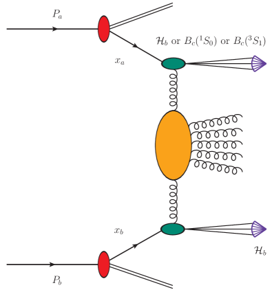
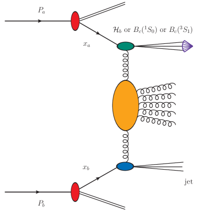
Figure 1: Hybrid collinear and high-energy factorization for double-hadron detection (left) and hadron-plus-jet inclusive hadroproduction (right). Collinear parton densities are represented by red ovals. The green (blue) blob depicts the off-shell hard factor embodied in the hadron (jet) emission function, while indigo arrows depicts the emission of $b$-flavored hadrons. The Green’s function is described by the orange blob. The diagram was created with JaxoDraw 2.0 [208].

We will study the two kinds of processes depicted in Fig. 1

$$\begin{split}{\rm p}(P_{a})\;+\;{\rm p}(P_{b})&\;\rightarrow\;{\cal B}_{1}(q_{1},y_{1},\phi_{1})\;+\;{\cal X}\;+\;{\cal B}_{2}(q_{2},y_{2},\phi_{2})\;,\\ {\rm p}(P_{a})\;+\;{\rm p}(P_{b})&\;\rightarrow\;{\cal B}(q_{1},y_{1},\phi_{1})\;+\;{\cal X}\;+\;{\rm jet}(q_{2},y_{2},\phi_{2})\;,\end{split}$$ (1)

where ${\rm p}(P_{a,b})$ is an initial-state proton possessing four-momentum $P_{a,b}$, from which a parton with longitudinal-momentum fraction $x_{a,b}$ is struck. Then, ${\cal B}_{(1,2)}(q_{1,2},y_{1,2})$ stands for a singly bottom-flavored hadron ${\cal H}_{b}\equiv\{B+\Lambda_{b}\}$, or a charmed-bottomed meson $B_{c}(^{1}S_{0})\equiv B_{c}$, or its resonance $B_{c}(^{3}S_{1})\equiv B_{c}^{*}$, emitted with four-momentum $q_{1,2}$, rapidity $y_{1,2}$ and azimuthal angle $\phi_{1,2}$, and a light-favored jet is possibly tagged with four-momentum $q_{2}$, rapidity $y_{2}$ and azimuthal angle $\phi_{2}$. Furthermore, ${\cal X}$ represents an inclusively radiated gluon system. The large final state transverse momenta, $|\vec{q}_{1,2}|$, together with the high rapidity interval, $\Delta Y\equiv y_{1}-y_{2}$, are required ingredients to make the final state be both semi-hard and diffractive. In addition, transverse momenta of the observed particles need to be enough high to make the VFNS fragmentation approach be valid.

Stemming protons’ four-momenta can be written as Sudakov vectors with the conditions $P_{a}^{2}=P_{b}^{2}=0$ and $2(P_{a}\cdot P_{b})=s$, so that final-state four-momenta are cast via the following decomposition

$$q_{1,2}=x_{1,2}P_{a,b}+\frac{\vec{q}_{1,2}^{\,2}}{x_{1,2}s}P_{b,a}+q_{1,2\perp}\ ,\quad q_{1,2\perp}^{2}=-\,\vec{q}_{1,2}^{\,2}\;.$$ (2)

The outgoing-object longitudinal-momentum fractions are labeled as $x_{1,2}$. They are connected with the respective rapidities and to $\Delta Y$ via

$$y_{1,2}=\pm\,\frac{1}{2}\ln\frac{s\,x_{1,2}^{2}}{\vec{q}_{1,2}^{2}}\;,\qquad{\rm d}y_{1,2}=\pm\,\frac{{\rm d}x_{1,2}}{x_{1,2}}\;,\qquad\Delta Y=\ln\frac{s\,x_{1}x_{2}}{|\vec{q}_{1}||\vec{q}_{2}|}\;.$$ (3)

According to the pure collinear factorization, one would write the LO cross section for our processes (Eq. (1)) as a one-dimensional convolution among the partonic-subprocess factor, proton PDFs, and $b$-hadron FFs. Considering the double hadron case as depicted in the left diagram of Fig. 1, we have

$$\begin{split}\frac{{\rm d}\sigma_{[p+p\,\to\,{\cal B}+{\cal B}]}^{\rm LO}}{{\rm d}x_{1}{\rm d}x_{2}{\rm d}^{2}\vec{q}_{1}{\rm d}^{2}\vec{q}_{2}}&=\sum_{i,j=-6}^{6}\int_{0}^{1}{\rm d}x_{i}\int_{0}^{1}{\rm d}x_{j}\ f_{i}(x_{i},\mu_{F})f_{j}(x_{j},\mu_{F})\\ &\times\,\int_{x_{1}}^{1}\frac{{\rm d}\xi_{1}}{\xi_{1}}\int_{x_{2}}^{1}\frac{{\rm d}\xi_{2}}{\xi_{2}}\ D^{{\cal B}_{1}}_{i}\left(\frac{x_{1}}{\xi_{1}},\mu_{F}\right)D^{{\cal B}_{2}}_{j}\left(\frac{x_{2}}{\xi_{2}},\mu_{F}\right)\frac{{\rm d}{\hat{\sigma}}_{ij}}{{\rm d}x_{i}{\rm d}x_{j}{\rm d}\xi_{1}{\rm d}\xi_{2}{\rm d}^{2}\vec{q}_{1}{\rm d}^{2}\vec{q}_{2}}\;,\end{split}$$ (4)

with the $i$ and $j$ indices running over parton species, $f_{i,j}(x_{1,2},\mu_{F})$ being the proton PDFs, $D^{{\cal B}_{1,2}}_{i,j}(x_{1,2}/\xi_{1,2}\equiv z_{1,2},\mu_{F})$ denoting $b$-hadron FFs, $x_{1,2}$ and $\xi_{1,2}$) respectively standing for incoming- and fragmenting-partons’ longitudinal fractions, and ${\rm d}\hat{\sigma}_{ij}$ representing the partonic cross section. Analogously, we write the following collinear-convolution formula for the $b$-hadron plus light-jet case depicted in the right diagram of Fig. 1

$$\begin{split}\frac{{\rm d}\sigma_{[p+p\,\to\,{\cal B}+{\rm jet}]}^{\rm LO}}{{\rm d}x_{1}{\rm d}x_{2}{\rm d}^{2}\vec{q}_{1}{\rm d}^{2}\vec{q}_{2}}&=\sum_{i,j=-6}^{6}\int_{0}^{1}{\rm d}x_{i}\int_{0}^{1}{\rm d}x_{j}\ f_{i}(x_{i},\mu_{F})f_{j}(x_{j},\mu_{F})\int_{x_{1}}^{1}\frac{{\rm d}\xi}{\xi}D^{{\cal B}}_{i}\left(\frac{x_{1}}{\xi}\right)\frac{{\rm d}{\hat{\sigma}}_{ij}}{{\rm d}x_{1}{\rm d}x_{2}{\rm d}\xi\,{\rm d}^{2}\vec{q}_{1}{\rm d}^{2}\vec{q}_{2}}\;.\end{split}$$ (5)

At variance with the collinear framework, to write the expression for the high-energy resummed cross section in the hybrid factorization, one first makes use of BFKL and then completes the picture by adding collinear PDFs and FFs. We suitably rewrite the differential cross section as a Fourier expansion in terms of azimuthal coefficients

$$\frac{{\rm d}\sigma^{\rm NLL/NLO^{+}}}{{\rm d}y_{1}{\rm d}y_{2}{\rm d}\vec{q}_{1}{\rm d}\vec{q}_{2}{\rm d}\phi_{1}{\rm d}\phi_{2}}=\frac{1}{2\pi^{2}}\left[\frac{1}{2}\,{\cal C}_{0}^{\rm NLL/NLO^{+}}+\sum_{n=1}^{+\infty}{\cal C}_{n}^{\rm NLL/NLO^{+}}\,\cos\left(n(\pi-\Phi)\right)\right]\,,$$ (6)

with $\Phi\equiv\phi_{1}-\phi_{2}$. The ${\cal C}_{n}^{\rm NLL/NLO^{+}}$ coefficients are calculated within the BFKL formalism at a full NLL accuracy. Making use of the $\overline{\rm MS}$ renormalization scheme [209], we obtain [210]

$$\begin{split}{\cal C}_{n}^{\rm NLL/NLO^{+}}&=\int_{0}^{2\pi}{\rm d}\phi_{1}\int_{0}^{2\pi}{\rm d}\phi_{2}\,\frac{{\rm d}\sigma^{\rm NLL/NLO^{+}}}{{\rm d}y_{1}{\rm d}y_{2}\,{\rm d}|\vec{q}_{1}|\,{\rm d}|\vec{q}_{2}|{\rm d}\phi_{1}{\rm d}\phi_{2}}\,\cos\left(n(\pi-\Phi)\right)\;\\ &=\;\frac{e^{\Delta Y}}{s}\int_{-\infty}^{+\infty}{\rm d}\nu\,e^{{\Delta Y}\bar{\alpha}_{s}(\mu_{R})\chi^{\rm NLO}(n,\nu)}\\ &\times\;\alpha_{s}^{2}(\mu_{R})\,\biggl{\{}{\cal E}_{1}^{\rm NLO}(n,\nu,|\vec{q}_{1}|,x_{1})\,[{\cal E}_{2}^{\rm NLO}(n,\nu,|\vec{q}_{2}|,x_{2})]^{*}\,+\,\left.\bar{\alpha}_{s}^{2}(\mu_{R})\,\Delta Y\frac{\beta_{0}}{4N_{c}}\chi(n,\nu){\cal F}(\nu)\right\}\;,\end{split}$$ (7)

where $\bar{\alpha}_{s}(\mu_{R})\equiv\alpha_{s}(\mu_{R})N_{c}/\pi$ with $N_{c}$ the color number, $\beta_{0}=11N_{c}/3-2n_{f}/3$ is the first coefficient of the QCD $\beta$-function with $n_{f}$ the flavor number. A two-loop running-coupling choice with $\alpha_{s}\left(M_{Z}\right)=0.118$ and with dynamic thresholds for the flavor number $n_{f}$ is made. The kernel entering the exponent of Eq. (7) encompasses the resummation of LL and NLL terms. Its analytic expression is

$$\chi^{\rm NLO}(n,\nu)=\chi(n,\nu)+\bar{\alpha}_{s}\hat{\chi}(n,\nu)\;,$$ (8)

where

$$\chi\left(n,\nu\right)=-2\gamma_{\rm E}-2\,{\rm Re}\left\{\psi\left(\frac{n}{2}+\frac{1}{2}+i\nu\right)\right\}\,$$ (9)

stand for the LO kernel eigenvalues, $\gamma_{\rm E}$ is the Euler-Mascheroni constant, and $\psi(z)\equiv\Gamma^{\prime}(z)/\Gamma(z)$ the Gamma-function logarithmic derivative. The $\hat{\chi}(n,\nu)$ function in Eq. (8) represents the NLO kernel correction in the Mellin space

$$\begin{split}\hat{\chi}\left(n,\nu\right)&=\bar{\chi}(n,\nu)+\frac{\beta_{0}}{8N_{c}}\chi(n,\nu)\left(\frac{10}{3}+\ln\frac{\mu_{R}^{4}}{m_{1\perp}^{2}m_{2\perp}^{2}}-\chi(n,\nu)\right)\;,\end{split}$$ (10)

where $m_{1,2\perp}$ are the transverse masses of the two outgoing states. For a $b$-hadron one has $m_{{\cal B}\perp}=\sqrt{m_{\cal B}^{2}+|\vec{q}_{\cal B}|^{2}}$, with $m_{\cal B}\equiv m_{{\cal H}_{b}}\equiv m_{\Lambda_{c}}=5.62$ GeV or $m_{\cal B}\equiv m_{B_{c}^{(*)}}=6.275$ GeV. Conversely, the transverse mass of a light-flavored jets can be safely set to transverse momentum, say $m_{{\cal J}\perp}\equiv|\vec{q}_{\cal J}|$. The NLO $\bar{\chi}(n,\nu)$ function was computed in Ref. [211]

$$\bar{\chi}(n,\nu)\,=\,-\frac{1}{4}\left\{\frac{\pi^{2}-4}{3}\chi(n,\nu)-6\zeta(3)-\frac{{\rm d}^{2}\chi}{{\rm d}\nu^{2}}+\,2\,\Xi(n,\nu)+\,2\,\Xi(n,-\nu)\right.$$ (11)

$$\left.+\;\frac{\pi^{2}\sinh(\pi\nu)}{2\,\nu\,\cosh^{2}(\pi\nu)}\left[\left(3+\left(1+\frac{n_{f}}{N_{c}^{3}}\right)\frac{11+12\nu^{2}}{16(1+\nu^{2})}\right)\delta_{n0}-\left(1+\frac{n_{f}}{N_{c}^{3}}\right)\frac{1+4\nu^{2}}{32(1+\nu^{2})}\delta_{n2}\right]\right\}\,.$$

The $\Xi(n,\nu)$ function reads

$$\Xi(n,\nu)\,=\,-\int_{0}^{1}{\rm d}x\,\frac{x^{-1/2+i\nu+n/2}}{1+x}\left\{\frac{1}{2}\left(\psi^{\prime}\left(\frac{n+1}{2}\right)-\zeta(2)\right)+\mbox{Li}_{2}(x)+\mbox{Li}_{2}(-x)\right.$$ (12)

$$\left.+\;\ln x\left[\psi(n+1)-\psi(1)+\ln(1+x)+\sum_{k=1}^{\infty}\frac{(-x)^{k}}{k+n}\right]+\sum_{k=1}^{\infty}\frac{x^{k}}{(k+n)^{2}}\left[1-(-1)^{k}\right]\right\}$$

$$=\;\sum_{k=0}^{\infty}\frac{(-1)^{k+1}}{k+(n+1)/2+i\nu}\left\{\psi^{\prime}(k+n+1)-\psi^{\prime}(k+1)\right.$$

$$\left.+\;(-1)^{k+1}\left[\rho(k+n+1)+\rho(k+1)\right]-\frac{\psi(k+n+1)-\psi(k+1)}{k+(n+1)/2+i\nu}\right\}\;,$$

with

$$\rho(z)=\frac{1}{4}\left[\psi^{\prime}\left(\frac{z+1}{2}\right)-\psi^{\prime}\left(\frac{z}{2}\right)\right]\;,$$ (13)

and

$$\mbox{Li}_{2}(z)=-\int_{0}^{z}{\rm d}\zeta\,\frac{\ln(1-\zeta)}{\zeta}\;.$$ (14)

The two quantities

$${\cal E}_{1,2}^{\rm NLO}(n,\nu,|\vec{q}_{1,2}|,x_{1,2})={\cal E}_{1,2}(n,\nu,|\vec{q}_{1,2}|,x_{1,2})+\alpha_{s}(\mu_{R})\,\hat{\cal E}_{1,2}(n,\nu,|\vec{q}_{1,2}|,x_{1,2})$$ (15)

stand for the emission functions of the forward $b$-hadron and the light jet. At LO one has

$$\begin{split}{\cal E}_{\cal B}(n,\nu,|\vec{q}_{\cal B}|,x_{\cal B})&=2\sqrt{\frac{C_{F}}{C_{A}}}|\vec{q}_{\cal B}|^{2i\nu-1}\,\int_{x_{\cal B}}^{1}\frac{{\rm d}\xi}{\xi}\left(\frac{\xi}{x_{\cal B}}\right)^{2i\nu-1}\left[\frac{C_{A}}{C_{F}}f_{g}(\xi)D_{g}^{\cal B}\left(\frac{x_{\cal B}}{\xi}\right)+\sum_{i=q,\bar{q}}f_{i}(\xi)D_{i}^{\cal B}\left(\frac{x_{\cal B}}{\xi}\right)\right]\end{split}$$ (16)

and

$${\cal E}_{\cal J}(n,\nu,|\vec{q}_{\cal J}|,x_{\cal J})=2\sqrt{\frac{C_{F}}{C_{A}}}|\vec{q}_{\cal J}|^{2i\nu-1}\,\left(\frac{C_{A}}{C_{F}}f_{g}(x_{\cal J})+\sum_{j=q,\bar{q}}f_{j}(x_{\cal J})\right)\;,$$ (17)

with $C_{F}\equiv(N_{c}^{2}-1)/(2N_{c})$ and $C_{A}\equiv N_{c}$ being the Casimir factors for a gluon emission from a quark and a gluon, respectively. The ${\cal F}(\nu)$ function at the end of the last row of Eq. (7) embodies the logarithmic derivative of LO emission functions

$${\cal F}(\nu)=\ln\left(|\vec{q}_{1}||\vec{q}_{2}|\right)+\frac{i}{2}\,\frac{{\rm d}}{{\rm d}\nu}\ln\frac{{\cal E}_{1}}{{\cal E}_{2}^{*}}\;.$$ (18)

What is left in Eq. (7) are the NLO corrections to ${\cal E}_{{\cal B},{\cal J}}$ functions, $\hat{\cal E}_{1,2}$. The NLO correction to the ${\cal B}$ hadron at large transverse momentum was computed in Ref. [124] and is provided in the Appendix A. Our choice for the jet NLO emission function builds on analyses described in Refs. [124, 126]. It relies upon a jet algorithm obtained in the “small-cone” limitand with a cone-type distance [212, 213, 127], where the radius is set to $r=0.5$ (see the Appendix B).

A proper “resummation versus fixed-order” study should rely upon comparing NLL predictions from our high-energy approach with NLO calculations in pure collinear factorization. Unfortunately, a numerical technology aimed at computing NLO distributions for two-particle reactions in hadron collisions is still missing. Thus, for the sake of comparison with reference fixed-order results, one can truncate the expansion of the azimuthal coefficients of Eq. (7) up to the ${\cal O}(\alpha_{s}^{3})$ order. In this way, one obtains an effective high-energy fixed-order (${\rm HE}\mbox{-}{\rm NLO^{+}}$) expression that collects the leading-power asymptotic signal present in a pure NLO calculation, whereas terms proportional by inverse powers of the partonic center-of-mass energy are neglected. The $\overline{\rm MS}$ expressions for ${\rm HE}\mbox{-}{\rm NLO^{+}}$ azimuthal coefficients reads

$${\cal C}_{n}^{{\rm HE}\text{-}{\rm NLO}^{+}}=\frac{e^{\Delta Y}}{s}\int_{-\infty}^{+\infty}{\rm d}\nu\,\alpha_{s}^{2}(\mu_{R})\,\left[1+\bar{\alpha}_{s}(\mu_{R})\Delta Y\chi(n,\nu)\right]\,{\cal E}_{1}^{\rm NLO}(n,\nu,|\bm{\kappa}_{1}|,x_{1})\,[{\cal E}_{2}^{\rm NLO}(n,\nu,|\bm{\kappa}_{2}|,x_{2})]^{*}\;,$$ (19)

with the exponentiated kernel expanded and truncated at ${\cal O}(\alpha_{s})$.

We will also compare our NLL results with the pure LL background. The latter is obtained by discarding NLO corrections of both the kernel and the emission functions

$${\cal C}_{n}^{\rm LL/LO}=\frac{e^{\Delta Y}}{s}\int_{-\infty}^{+\infty}{\rm d}\nu\,e^{{\Delta Y}\bar{\alpha}_{s}(\mu_{R})\chi(n,\nu)}\,\alpha_{s}^{2}(\mu_{R})\,{\cal E}_{1}(n,\nu,|\vec{q}_{1}|,x_{1})\,[{\cal E}_{2}(n,\nu,|\vec{q}_{2}|,x_{2})]^{*}\,.$$ (20)

Eqs. (7) to (20) shed light on the structure of our hybrid factorization. According to BFKL, the cross section is high-energy factorized as a convolution between the Green’s function and two singly off-shell emission functions. The latters embody collinear inputs, namely collinear convolutions between incoming protons’ PDFs and outgoing hadrons’ FFs. The ${\rm NLL/NLO^{+}}$ label tells us that the resummation of energy logarithms is performed within a full NLL accuracy and within NLO perturbative order. The ‘$+$’ superscript in Eqs. (7) and (19) highlights that some NNLL extra terms come from the cross product between NLO corrections of the two emission functions. Finally, factorization ($\mu_{F}$) and renormalization ($\mu_{R}$) scales are set to the natural scales suggested by kinematics. In particular, we fix $\mu_{F}=\mu_{R}=\mu_{N}\equiv m_{1\perp}+m_{2\perp}$.

2.3 Collinear inputs

As for collinear PDFs, we make use of the NNPDF40_nlo_as_01180 NLO set [214, 215] as implemented in LHAPDF v6.5.4 [216]. It was obtained on the basis of global fits by means of the well-defined replica methodology originally proposed in Ref. [217] in the context of a neural-network approach (we refer to Ref. [218] for an in-depth analysis on ambiguities about correlations among different PDF sets).

Parton fragmentation to singly-bottomed ${\cal H}_{b}\equiv\{B+\Lambda_{b}\}$ hadrons is depicted via the KKSS07 NLO FF determination, which was originally obtained by fitting data on inclusive productions of noncharmed $B$ mesons in lepton annihilation [55]. Here, the threshold for bottom- and antibottom-quark evolution is set to 4.5 GeV and its initial-scale parametrization reads as a power-like function with three parameters [219]. Light partons and the charm quarks are perturbatively generated with DGLAP, while their FFs are zero below the threshold for the bottom. The current KKSS07 set [57] for ${\cal H}_{b}$ particles was constructed from the original noncharmed $B$-meson ones by switching off the branching fraction for the $b\to B^{\pm}$ subprocess, which was assumed to be $f_{u}=f_{d}=0.397$ [55]. Such a choice is justified by the assumption that a unique function can be employed in the description of noncharmed $B$-meson fragmentation or of an inclusive sum of $B$ and $\Lambda_{b}$ channels, but not for the $\Lambda_{b}$-baryon case alone.

Our strategy for charmed $B$-meson fragmentation is more involved. It was presented for the first time in our recent study focused on accessing the high-energy spectrum of QCD via the hadroproduction of these doubly heavy-flavored states [83]. It takes inspiration from a first determination of VFNS, DGLAP-evolving FFs for vector quarkonia [84, 85]. The starting point is the NLO calculation, within the NRQCD effective theory, of initial-scale inputs for charm, bottom quark [81] and gluon [82] fragmentation channels to $B_{c}(^{1}S_{0})\equiv B_{c}$ and $B_{c}(^{3}S_{1})\equiv B_{c}^{*}$ mesons (see Refs. [220, 221] for similar calculations). To generate DGLAP-evolved sets for our charmed $B$ mesons we need to plug the NRQCD inputs into a numeric evolution code. Among them, we cite: QCD-PEGASUS [222], HOPPET [223], QCDNUM [224], APFEL(++) [225, 226, 227], and EKO [228, 229]. Contrariwise to PDFs, which obey a space-like evolution equation, FFs must be time-like evolved [230, 231]. In Ref. [83] we employed APFEL++ to generate novel and phenomenology-ready LHAPDF FF grids, which we named ZCFW22 NLO determinations.

For the sake of comparison, we employ the NNFF10_KAsum_nlo set [232] (see Ref. [233] for advancements) to describe charged-kaon fragmentation at NLO.

2.4 Natural stabilization of the NLL series

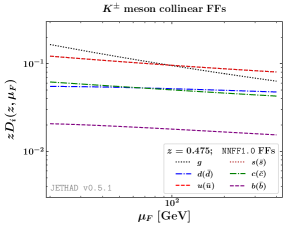
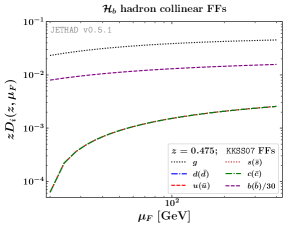
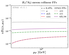
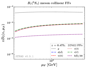
Figure 2: Factorization-scale dependence of NNFF1.0 [232], KKSS07 [55, 57], and ZCFW22 [83] NLO FFs respectively describing: kaon (upper left panel), ${\cal H}_{b}$ hadron (upper right panel), and charmed $B$ meson (lower panels) detections, for $\langle z\rangle\simeq 0.475$.

Here we provide details on the stabilizing mechanism emerging from the VFNS collinear fragmentation of $b$-hadrons. The linking dynamics between heavy-flavor FFs and the observed stability of semi-inclusive distributions calculated within the hybrid collinear and high-energy factorization at ${\rm NLL/NLO^{(+)}}$ was first unveiled through a study of semi-hard emissions of heavy-light hadrons, namely: $D$ particles [234, 235, 236, 237, 238, 239, 240, 241, 242], $\Lambda_{c}$ baryons [235, 243, 244], and ${\cal H}_{b}$ states [54, 245, 55, 56, 246, 57, 59, 247, 248]. This striking property came out for the first time from an analysis of semi-inclusive detections of $\Lambda_{c}$ [162, 90], $D^{*\pm}$ [165, 164], and ${\cal H}_{b}$ [163, 90] hadrons in forward directions of rapidity at the LHC. Such a remarkable result was then corroborated by similar investigations on vector quarkonia [84, 249] and $B_{c}^{(*)}$ mesons [83], whose formation mechanism was modeled on the basis of single-parton NRQCD fragmentation [250, 251, 252, 253, 254, 255, 81, 82, 220, 221]. A further evidence came recently out in the context of heavy-light tetraquarks [207] described via a Suzuki–Nejad–Amiri–Ji initial-scale fragmentation input [256, 257, 258, 259] (see Refs. [260, 261] for further details). A less pronounced stabilization pattern was also observed in the case of strange-quark flavored, cascade $\Xi^{-}/\bar{\Xi}^{+}$ baryon tags [159].

Panels in Fig. 2 contain the factorization-scale dependence of KKSS07 [55, 57] and ZCFW22 [83] NLO functions respectively describing the collinear fragmentation of ${\cal H}_{b}$ hadrons (right upper plot) and $B_{c}^{(*)}$ mesons (lower plots). For comparison, the left upper plot carries analogous information of light-quark flavored species, namely charged kaons, described by the NNFF1.0 [232] NLO collinear-FF determination. For the sake of simplicity, we show values of our FF sets just for one value of the final-state hadron longitudinal-momentum fraction, $z$. In particular, we choose a value of $z$ that roughly matches the mean value at which FFs are typically probed standard semi-hard configurations (see Section 3.2). Thus we have $z=0.475\simeq\langle z\rangle$. As expected, the $b$ channel of KKSS07 and ZCFW22 functions heavily prevails over the other flavors. Particular attention deserves, however, the behavior the gluon FF, which clearly decreases with $\mu_{F}$ for kaons but smoothly increases for all the three $b$-flavored species, up to reach a plateau.

As extensively shown in Refs. [111, 162, 163, 84, 83, 207], the gluon collinear FF plays a crucial role. De facto, it has a strong stabilization power on our ${\rm NLL/NLO^{+}}$ observables. Its behavior with $\mu_{F}$ fairly controls the stability of the high-energy logarithmic series of our distributions. In the semi-hard regime proton PDFs are typically probed at $10^{-4}\lesssim x\lesssim 10^{-2}$, where the gluon PDF heavily dominates over quark ones. Given that the gluon FF diagonally multiplies with the gluon PDF in the LO hadron emission function (see Eq. (16)), its impact on the cross section is magnified. This effect is not quenched at NLO, where $\{qg\}$ and $\{gq\}$ nondiagonal channels are opened [162] (see the Appendix A). On one side, $\alpha_{s}$ decreases with $\mu_{R}$ both in the Green’s function and in the emission functions (see Section 2.2). At the same time, however, the gluon PDF increases as $\mu_{F}$ enlarges. When that density multiplies a gluon FF which also increases with $\mu_{F}$, as it happens for $b$-hadrons, the two effects balance each other. This leads to the stabilizing trend of heavy-flavor distributions under energy-scale variations. If instead the gluon FF falls down with $\mu_{F}$, as it happens for light-flavored species, such charged kaons, the stabilizing pattern is lost. This harms any chance of making precision tests of semi-hard observables at the natural energies given by kinematics [87]. The emergence of the natural stability [111] in presence of both singly a doubly heavy flavored hadron species provides us with clear evidence that this striking feature is an intrinsic property of heavy-flavor detections, which becomes manifest whenever a heavy hadron emitted, independently of the choice made for the initial-scale input of the corresponding collinear fragmentation.

3 Hi-Lumi LHC distributions

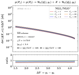
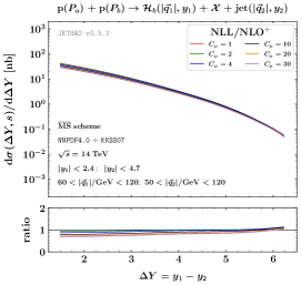
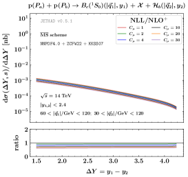
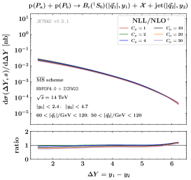
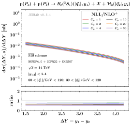
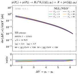
Figure 3: $\Delta Y$-rate of the double-hadron (left) and the hadron-plus-jet (right) channel at $\sqrt{s}=14$ TeV and within the ${\rm NLL/NLO^{+}}$ accuracy. Renormalization and factorization scales are progressively varied in the $1<C_{\mu}<30$ range.

We performed our numeric computations via the Jethad v0.5.1 interface [87, 90, 85], a Python+Fortran multimodular working environment aimed at the calculation, management, and processing of high-energy distributions obtained from different theoretical approaches. In particular, rapidity and transverse-momentum differential cross sections were calculated by means of Jethad Fortran 2008 core modules, whereas its Python 3.0 analyzer was used to elaborate results. Section 3.1 gives details on our procedure to gauge the size of uncertainties for our resummed observables. Final-state kinematic cuts are presented in Section 3.2. Then, Section 3.3 carries a discussion of our ${\rm NLL/NLO^{+}}$ predictions.

3.1 Uncertainty estimation

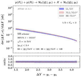
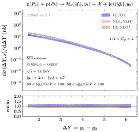
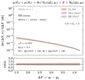
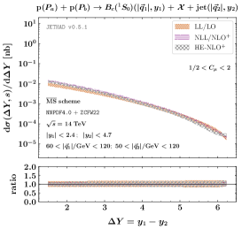
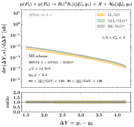
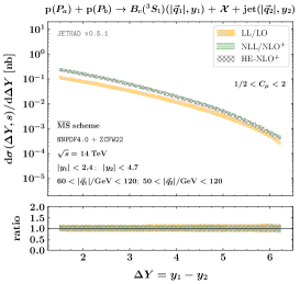
Figure 4: $\Delta Y$-rate of the double-hadron (left) and the hadron-plus-jet (right) channel at $\sqrt{s}=14$ TeV and within the ${\rm NLL/NLO^{+}}$ accuracy. Shaded bands exhibit the combined effect of renormalization- and factorization-scale variation in the $1<C_{\mu}<2$ range.

A widely-used methodology to quantify the weight of MHOUs relies upon assessing how much our observables are sensitive to variations of factorization and renormalization scales around their natural values. It is well-known that the effect MHOUs gives perhaps the major contribution to the overall uncertainty [90]. For this reason, we will gauge the size of simultaneously varying $\mu_{F}$ and $\mu_{R}$ around $\mu_{N}/2$ and $2\mu_{N}$. The $C_{\mu}$ parameter in panels of figures of Sections 3.3 and 3.4 is just the $C_{\mu}\equiv\mu_{F}/\mu_{N}=\mu_{R}/\mu_{N}$ ratio. Another possibly relevant uncertainty is encoded in proton PDFs. Quite recent analyses on high-energy production rates have shown, however, that selecting distinct PDF parametrizations as well as distinct members inside the same set produces a very small effect [155, 87, 163, 90]. Therefore, we will calculate our observables by considering only the central member of the NNPDF4.0 parametrization. Then, other potential uncertainties could come from a collinear improvement of the NLO kernel (see Refs. [262, 263, 264] and reference therein), which consists in including renormalization-group (RG) terms to make the BFKL equation compatible with the DGLAP one in the collinear limit, or from changing the renormalization scheme. The first case was deeply addressed in Ref. [90]. As a result, the impact of collinear-improvement techniques on rapidity-differential rates is fairly contained inside error bands produced by MHOUs, and it is even smaller in the case of when other differential observables. The same article provides us with an overestimation of the effect of passing from $\overline{\rm MS}$ [209] to MOM [265, 266] renormalization scheme. MOM results for rapidity distributions are systematically higher than $\overline{\rm MS}$ ones, but still contained into MHOU bands. We stress, however, that a proper MOM analysis should be based on MOM-evolved PDFs and FFs, not available so far.

We will produce uncertainty bands for our distributions by combining MHOUs with the numeric error generated by the multidimensional integration (see Section 3.2). The latter will be constantly kept below $1\%$ by the Jethad integration subinterfaces.

3.2 Kinematic constraints on final-state ranges

We will consider two main observables: $(i)$ the rapidity-interval distribution, namely the cross section differential in the rapidity separation, $\Delta Y=y_{1}-y_{2}$, between the two produced particles, and $(ii)$ the doubly-differential transverse-momentum distribution.

The first observable genuinely corresponds the ${\cal C}_{0}$ azimuthal-angle coefficient, defined in Section 2.2, integrated over final-state transverse momenta and rapidities and taken at fixed values of $\Delta Y$

$$\frac{{\rm d}\sigma(\Delta Y;s)}{{\rm d}\Delta Y}=\int_{|\vec{q}_{2}|^{\rm min}}^{|\vec{q}_{2}|^{\rm max}}\!\!{\rm d}|\vec{q}_{1}|\int_{|\vec{q}_{2}|^{\rm min}}^{|\vec{q}_{2}|^{\rm max}}\!\!{\rm d}|\vec{q}_{2}|\int_{\max\,(y_{1}^{\rm min},\,\Delta Y+y_{2}^{\rm min})}^{\min\,(y_{1}^{\rm max},\,\Delta Y+y_{2}^{\rm max})}{\rm d}y_{1}\,\,{\cal C}_{0}^{\rm[order]}\left(|\vec{q}_{1}|,|\vec{q}_{2}|,y_{1},y_{2};s\right)\Bigm{\lvert}_{y_{2}\;=\;y_{1}-\Delta Y}\;,$$ (21)

where the ‘${\rm[order]}$’ label for ${\cal C}_{0}$ inclusively refers to: ${\rm NLL/NLO^{+}}$, ${\rm HE}\mbox{-}{\rm NLO^{+}}$, or ${\rm LL/LO}$. Here we made use of a $\delta(\Delta Y-y_{1}+y_{2})$ function to remove the integration over one of the two rapidities, say $y_{2}$. Transverse momenta of the forward $b$-hadron and the backward one stay in the ranges $60<|\vec{q}_{1}|/{\rm GeV}<120$ and $30<|\vec{q}_{2}|/{\rm GeV}<120$, respectively. These cuts fairly meet the criteria of applicability of a VFNS-based fragmentation approach, in which energy scales must be sufficiently higher than thresholds for the DGLAP evolution of heavy-quark species. Then, light jets are tagged in transverse-momentum ranges lightly different but compatible with current and forthcoming studies at the LHC [267], say $50<|\vec{q}_{2}|/\rm{GeV}<60$. The use of such asymmetric transverse-momentum ranges eases disentangling the pure high-energy dynamics from the fixed-order signal [142, 143, 87]. It also dampens large Sudakov logarithms due to almost back-to-back configurations which would require the employment of another resummation [268, 269, 270, 271, 272, 273]. Finally, it quenches instabilities connected to radiative corrections [274, 275] as well as violations of the energy-momentum conservation relation [276]. As for the rapidity ranges, we select typical cuts of current LHC studies, where hadrons are detected only in the barrel calorimeter [277], say from $-2.4$ to $2.4$, whereas the jet can be also tagged in endcaps’ regions [267], say from $-4.7$ to $4.7$.

The second observable is given by the ${\cal C}_{0}$ azimuthal-angle coefficient, integrated over rapidities while $\Delta Y$ is kept fixed, but this time being differential in the transverse momenta of the two outgoing objects

$$\frac{{\rm d}\sigma(|\vec{q}_{1}|,|\vec{q}_{2}|,\Delta Y;s)}{{\rm d}|\vec{q}_{1}|{\rm d}|\vec{q}_{2}|{\rm d}\Delta Y}=\int_{\max\,(y_{1}^{\rm min},\,\Delta Y+y_{2}^{\rm min})}^{\min\,(y_{1}^{\rm max},\,\Delta Y+y_{2}^{\rm max})}{\rm d}y_{1}\,\,{\cal C}_{0}^{\rm[order]}\left(|\vec{q}_{1}|,|\vec{q}_{2}|,y_{1},y_{2};s\right)\Bigm{\lvert}_{y_{2}\;=\;y_{1}-\Delta Y}\;.$$ (22)

Here we consider the previously mentioned kinematic cuts for rapidities, whereas the two transverse momenta can run from 10 to 100 GeV. This observable was recently proposed, in the context of singly bottom-flavored hadrons [163] and cascade $\Xi$ baryons [159], as a favorable testing ground whereby unraveling the interplay among distinct resummations.

3.3 Rapidity-interval distributions

In Fig. 3 we present rapidity-interval distributions for our reference processes, calculated within ${\rm NLL/NLO^{+}}$ hybrid factorization and taken at $\sqrt{s}=14$ TeV. Left plots refer to double-hadron channels, while right plots are for the hadron-jet ones. Final states with ${\cal H}_{b}$ hadrons, $B_{c}(^{1}S_{0})$ mesons, or $B_{c}(^{3}S_{1})$ resonances are considered in upper, central, and lower plots, respectively. More in particular, any forward $b$-flavored hadron is always accompanied by a singly bottomed hadron ${\cal H}_{b}$ (left plots) or by a light-flavored jet (right plots). This is to avoid the presence of two identified charmed $B$ mesons in the final state, which would lead to a substantial lowering in statistics. We will adopt this choice also in the next Section (3.4). The minimum values of our distributions are the ones obtained at the maximum values of $\Delta Y$. They are uniformly larger than $10^{-2}$ nb when only ${\cal H}_{b}$ hadrons (and light jets) are produced, and larger than $10^{-5}$ nb in the two $B_{c}^{(*)}$ cases. This represents a very promising statistics that can be easily accessed via dedicated experimental studies at the forthcoming Hi-Lumi upgrade of the LHC. The decreasing trend with $\Delta Y$ of our NLL-resummed distributions is a general feature shared by all the semi-hard hadroproduction final states investigated so far. It comes out as the interplay between two competing effects. Indeed, although the high-energy dynamics encoded in the partonic hard factor would make the cross section grow with energy, collinear PDFs and FFs fall off very fast with $\Delta Y$, since this kinematically translates to longitudinal-momentum fractions very close to one. The net result is a dampening effect with $\Delta Y$ of hadronic distributions.

The core analysis shown in Fig. 3 is a study of our rapidity-interval differential distributions under a progressive variation of factorization and renormalization scales in an broad window, controlled by the $C_{\mu}$ parameter introduced in Section 3.1, which ranges from $1$ to $30$. This strategy actually represents an extended MHOU scan with respect to the traditional one, $1/2<C_{\mu}<2$. Ancillary panels drawn right below primary ones show reduced distributions, namely the ones divided by their central values calculated at $C_{\mu}=1$. Remarkably, ${\rm NLL/NLO^{+}}$ results for all the six considered final states feature quite a weak sensitivity on $C_{\mu}$ variation in the whole spectrum of $\Delta Y$ matter of our investigation. This supports the important message that a strong stabilization mechanism is encoded both in the KKSS07 functions extracted from global data on $B$ mesons and $\Lambda_{b}$ baryons, as well as in the novel ZCFW22 FFs built on the basis of NRQCD initial-scale inputs for $B_{c}(^{1}S_{0})$ and $B_{c}(^{3}S_{1})$ generalized-quarkonium states and then evolved via DGLAP in a VFNS scheme. Results contained in plots of Fig. 3 bring to light the emergence of the natural stability [111] from semi-inclusive $b$-flavor emissions at high energies.

As a complement, in Fig. 4 we show results for the same $\Delta Y$-distributions, calculated within the ${\rm NLL/NLO^{+}}$ accuracy and compared with ${\rm HE}\mbox{-}{\rm NLO^{+}}$ and ${\rm LL/LO}$ corresponding ones. Left (right) plots are for hadron-plus-hadron (hadron-plus-jet) observables. Upper, central, and lower plots respectively correspond to ${\cal H}_{b}$, $B_{c}$, and $B_{c}^{*}$ sensitive final states. This time, shaded bands are built by combining the uncertainty of the multidimensional integration, numerically performed by the Jethad integrators, with the one coming from a traditional MHOU scan, namely with the $C_{\mu}$ parameter running from 1/2 to two. As done before, lower ancillary panels exhibit reduced distributions, i.e. divided by central values calculated when $C_{\mu}=1$. The global outcome is a strong stability under higher-order corrections. This is confirmed by the fact that ${\rm NLL/NLO^{+}}$ uncertainty bands are generally narrower and partially nested inside corresponding ${\rm LL/LO}$ ones, in particular in the large-$\Delta Y$ regime, where the impact of high-energy logarithms is expected to be large. Their overlap is slightly weaker for hadron-plus-jet cases (right plots). This is not unexpected, since the emission of just one $b$-hadron rather then two reduces the stabilizing power by one half.

As discussed in previous works (see, e.g. Section 3 of Ref. [83]), shaded bands for fixed-order ${\rm HE}\mbox{-}{\rm NLO^{+}}$ results are almost completely nested in resummed ${\rm NLL/NLO^{+}}$ ones. Future analyses on more exclusive observables, such as angularity distributions will shed light on a clearer disentanglement between our resummation and the fixed-order signal. Finally, as a bonus result, we confirm the estimate, provided by the LHCb Collaboration [69, 70], on the production-rate hierarchy between singly-bottomed hadrons and charmed $B$ mesons. Production rates of the latters seems not to exceed 0.1% of the ${\cal H}_{b}$ ones, at most. To compare our predictions with these numbers, we can consider the hadron-plus-jet channel (right diagram of Fig. 1) at ${\rm LL/LO}$, whose differential cross section is linear in the $b$-hadron FFs (see Eq. (16)). The inspection of right plots of Fig. 4 in clearly in line with LHCb estimates for charmed $B$-meson sates. The hierarchy remains de facto unaltered both at ${\rm NLL/NLO^{+}}$ and at ${\rm HE}\mbox{-}{\rm NLO^{+}}$. Remarkably, this fact not only represents a reliability test for our hybrid factorization, but it also definitely corroborates the validity of the single-parton fragmentation mechanism from NRQCD, at least for the $B_{c}(^{1}S_{0})$ case.

3.4 Doubly-differential transverse-momentum distributions

Rapidity-interval distributions represent golden channels to unveil the onset of high-energy dynamics at hadron colliders. At the same time, pursuing the goal of exploring kinematic corners where other resummations are also at work, we need more differential observables in the transverse momentum. From one side, high transverse momenta or large imbalances between them heighten the size of DGLAP-type logarithms as well as soft, threshold ones [278, 279, 280, 281, 282, 283, 284, 285, 286, 287, 288, 289, 290, 291, 292, 293, 294, 295, 296, 297]. These logarithms, which are of a different nature with respect the high-energy ones, must also be resummed. From the other side, low transverse momenta translate into large Sudakov logarithms which are also missed by our hybrid factorization. Furthermore, effects connected to the well-known diffusion pattern rise [298, 299, 300]. The most natural way to catch these logarithms to all orders builds on the TM resummation formalism [301, 302, 303, 304, 305, 306, 307, 308].

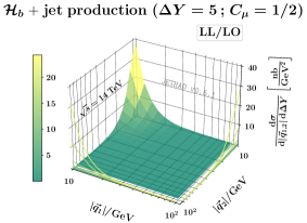
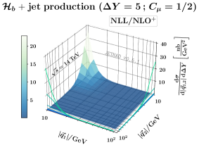
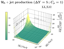
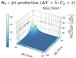
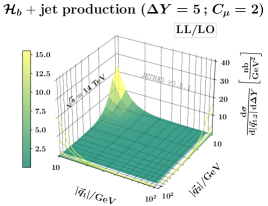
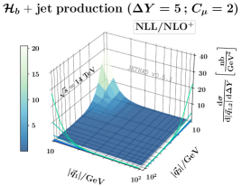
Figure 5: Doubly-differential transverse-momentum distribution for the ${\cal H}_{b}$-plus-jet production at $\Delta Y=5$, $\sqrt{s}=14$ TeV, and within the ${\rm LL/LO}$ (left) and ${\rm NLL/NLO^{+}}$ (right) accuracy. The $C_{\mu}$ scale parameter goes from 1/2 (top) to 2 (bottom).

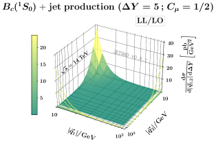
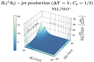
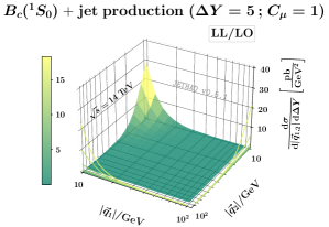
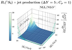
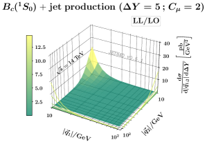
Figure 6: Doubly-differential transverse-momentum distribution for the $B_{c}(^{1}S_{0})$-plus-jet production at $\Delta Y=5$, $\sqrt{s}=14$ TeV, and within the ${\rm LL/LO}$ (left) and ${\rm NLL/NLO^{+}}$ (right) accuracy. The $C_{\mu}$ scale parameter goes from 1/2 (top) to 2 (bottom).

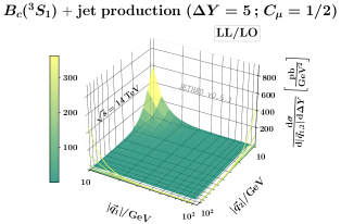
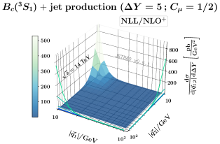
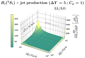
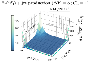
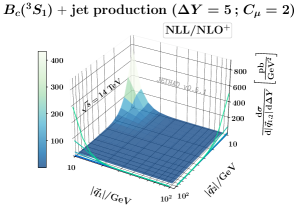
Figure 7: Doubly-differential transverse-momentum distribution for the $B_{c}(^{1}S_{0})$-plus-jet production at $\Delta Y=5$, $\sqrt{s}=14$ TeV, and within the ${\rm LL/LO}$ (left) and ${\rm NLL/NLO^{+}}$ (right) accuracy. The $C_{\mu}$ scale parameter goes from 1/2 (top) to 2 (bottom).

Inclusive emissions of two-particle final states in proton collisions, such as photon [309, 310, 311, 312], Higgs [313] and $W^{\pm}$ boson [314] pairs, as well as boson plus jet [315, 316] and $Z$ plus photon [317] systems, were proposed as favorable channels whereby testing the TM resummation. TM third-order fiducial rates for Drell–Yan and Higgs tags were respectively investigated in Refs. [318, 319, 320, 321] and [322, 323, 319, 324]. Ref. [315] presents a pioneering joint resummation of TM logarithms rising from the emission of two states. There, the simultaneous measurement of transverse momenta of the Higgs boson and the leading jet was analyzed up to the NNLL accuracy by means of the RadISH numeric technology [322]. Ref. [325] deals with a study of TM distributions for the fully leptonic $(W^{+}W^{-})$ tag at the LHC.

Heavy-flavor distributions bring to a further complication. Indeed, when the transverse momentum of a heavy hadron diminishes, its transverse mass comes closer and closer to heavy-quark masses serving as DGLAP thresholds, even crossing then when energy scales are moved below their natural values (as an example, this happens when the $C_{\mu}$ parameter introduced in Section 3.1 is set to 1/2). In this case, the validity of a pure VFNS approach becomes questionable.

In this Section we consider cross sections at fixed values of $\Delta Y$ and differential in the transverse momenta of both the final-state objects. In the kinematic sectors matter of our investigations energy logarithms arising from the semi-hard scale hierarchy are large. At the same time, however, also TM logarithms are potentially sizable. Therefore, we propose this study without pretension of catching the core features of these observables thanks to our hybrid-factorization framework, but rather to set the stage for futures analyses aimed at shedding light on the formal and phenomenological connection among distinct resummation mechanisms. Figures presented here are for doubly differential transverse-momentum distributions at $\Delta Y=5$. For the sake of simplicity, we present the hadron-plus-jet channel only (right diagram of Fig. 1). Predictions for singly bottomed hadrons, $B_{c}(^{1}S_{0})$ mesons, and their $B_{c}(^{3}S_{1})$ resonances are shown in surface 3D plots of Figs. 5, 6, and 7, respectively.

The common trend is a sharp falloff pattern when the two transverse momenta, $|\vec{q}_{1}|$ and $|\vec{q}_{2}|$, increase or when their mutual distance grows. ${\rm LL/LO}$ cross sections (left plots) are much more sensitive to MHOU studies done through energy-scale variations than ${\rm NLL/NLO^{+}}$ ones. They generally lower with $C_{\mu}$ (from upper to lower plots). ${\rm NLL/NLO^{+}}$ distributions (right panels) instead generally oscillate around $C_{\mu}=1$, which turns out to work as a critical point. This is a clear signal that our ${\rm NLL/NLO^{+}}$ doubly-differential cross sections are quite stable under MHOU analyses. Notably, no distribution comes with a peak, which might however be present in the low-TM range (excluded from our study), where TM-resummation effects would dominate. The information contained in the core of our 3D figures is supplemented by 2D slice projections highlighting the behavior of our observables at $|\vec{q}_{1}|=0$ and at $|\vec{q}_{2}|=0$. What emerges from the inspection of these 2D contour plots at low or intermediate transverse momentum is a smaller statistics in the $|\vec{q}_{1}|>|\vec{q}_{2}|$ range than in the opposite case. This happens because cross sections are globally smaller when a bottomed hadron is produced rather than a light-flavored jet [163, 83].

Finally, numeric checks on our transverse-momentum distributions have shown a noncharmed versus charmed $B$-meson production-rate hierarchy analogous to the one found in the case of rapidity-interval distributions (see Section 3.3). $B_{c}$ production rates are almost always three orders of magnitude smaller than ${\cal H}_{b}$ ones, whereas rates of the $B_{c}^{*}$ resonance range from $10^{-2}$ to $1/60$ times the ones of ${\cal H}_{b}$ hadrons.

4 Summary and Outlooks

We considered the semi-inclusive production of a forward noncharmed or charmed $b$-hadron in association with a backward noncharmed $b$-hadron or a jet in high-energy regimes that can be accessed at current LHC analyses and its forthcoming Hi-Lumi upgrade. We depicted the production of bottom-flavored hadrons by means of a VFNS collinear-fragmentation approach, whose validity is justified by the large transverse-momentum regime matter of our analysis.

Singly heavy-flavored particles, namely inclusive states consisting of $B$ mesons and $\Lambda_{b}$ baryons, were described via the KKSS07 [55, 57] NLO FFs based on a fit to global data and assuming a three-parameter power-like initial-scale parametrization for $b$ and $\bar{b}$ fragmentation channels [219]. As for charmed $B$ mesons, i.e. $B_{c}\equiv B_{c}(^{1}S_{0})$ states and $B_{c}^{*}\equiv B_{c}(^{3}S_{1})$ resonances, we adopted a more sophisticated strategy. First, we modeled the initial-scale input for the fragmentation of heavy quarks (charm, bottom, and their antiparticles) and gluons to observed hadrons by means of corresponding NLO calculations within the NRQCD effective theory [220, 221]. Then, we plugged these inputs into the APFEL(++) DGLAP evolution code [225, 226, 227] to generate phenomenology-ready VFNS FF grids in LHAPDF format [216], which we named ZCFW22 NLO functions [83]. These novel FF sets will play a role in future phenomenological applications lying outside the semi-hard regime. They also will serve as a support basis to shed light on the intersection corner between the collinear factorization and the NRQCD formalism.

By relying upon a traditional as well as an extended MHOU scan on our hybrid-factorization setup, we hunted for clues of stabilization of the high-energy resummation under next-to-leading logarithmic corrections. We provided strong evidence that these effects are present and they allow for a fair description of high-energy distributions, differential in the rapidity interval and in the final-state transverse momenta. As a bonus, we highlighted that the predicted production-rate hierarchy between noncharmed $b$-hadrons and charmed $B_{c}(^{1}S_{0})$ mesons is in line with recent LHCb estimates. In particular, the production rate of $B_{c}$ states is three orders of magnitude lower than the ${\cal H}_{b}$ one. This served as a simultaneous benchmark for both the hybrid factorization and the NRQCD fragmentation applied to charmed $B$ mesons at our reference transverse masses (see Section 3.2).

Our analysis on bottom-flavor collinear fragmentation stands as a step forward in the study of heavy-flavored emissions within the ${\rm NLL/NLO^{(+)}}$ accuracy, originally started from the analytic calculation of singly off-shell emission functions depicting the production of heavy-quark pairs in the moderate-to-low transverse-momentum regime [134, 161, 136]. It also represents a fair contact point with phenomenology of bottom-flavor production in the high-energy sector. The extension of this study to wider kinematic ranges, like the ones typical of new-generation colliding machines [326, 327, 328, 329, 330, 331, 332, 333, 334, 335, 336, 337, 338, 339, 340, 341, 342, 343, 344, 345], as well as possible contact points with heavy-flavor fragmentation studies in the TMD formalism [346, 347, 348, 349, 350, 351], is underway.

As a prospect, we plan to investigate bottom-flavor emissions in the moderate transverse-momentum sector, namely at the intersection line between the VFNS and the FFNS scheme, and possibly set the stage for a matching between the two descriptions. Here, high-energy tags of charmed $B$ mesons will bring novelty to the plan. In that case, indeed, the VFNS versus FFNS dichotomy translates into a short-distance versus fragmentation dichotomy. This calls for a further enhancement of our ZCFW22-based treatment, which currently relies upon NRQCD-modeled calculations for initial-scale inputs, but will serve in the medium-term future as a “launch pad” for extractions through fits to new data to be collected at the Hi-Lumi LHC. In this respect, neural-network strategies already employed to extract collinear FFs for lighter hadron species will be an asset [352, 353, 232, 233, 354, 355]. A proper determination of FF uncertainties with possible inclusion of MHOU effects, not yet encoded in our ZCFW22 sets, might take inspiration from the MCscales approach [356] (for a close-in-spirit study on pion PDFs, see Ref. [357]).

The fair stability exhibited by our ${\rm NLL/NLO^{+}}$ distributions motivates our interest in proposing the hybrid factorization as useful tool to enhance and extend the standard collinear description. To reach the precision level, our ${\rm NLL/NLO^{+}}$ hybrid approach needs to evolve into a multi-lateral formalism where different resummation mechanisms are at work. As a first steps, links with the soft-gluon [272, 273, 358, 359] and the jet-radius [360, 361, 362, 363, 364] resummations should be found. Possible common grounds with studies on jet angularities [365, 366, 367] also represent an intriguing perspective.

Then, the resummation of energy logarithms from BFKL could improve the description of DGLAP-evolved bottom-flavor FFs, its effect becoming sizable already at moderate values of final-state hadron longitudinal fraction [368]. Finally, the striking evidence of intrinsic charm quarks in the proton [369], now corroborated by quite recent studies on its valence distribution [370], traces the path towards searches for imprints of the possible existence of an intrinsic bottom component. In this respect, any progress in widening the horizons of our knowledge of bottom physics is needed. We believe that studies aimed at shedding light on the bottom-flavor collinear fragmentation go along these directions.

Appendix A: NLO $b$-hadron emission function

In this Appendix we provide the expression of the NLO correction for the emission function of a forward $b$-hadron tagged at large transverse momentum (see Ref. [124] for technical details). We write

$$\hat{\cal E}_{\cal B}(n,\nu,|\vec{q}_{\cal B}|,x_{\cal B})=\frac{1}{\pi}\sqrt{\frac{C_{F}}{C_{A}}}\left(|\vec{q}_{\cal B}|^{2}\right)^{i\nu-\frac{1}{2}}\int_{x_{\cal B}}^{1}\frac{{\rm d}x}{x}\int_{\frac{x_{\cal B}}{x}}^{1}\frac{{\rm d}\tau}{\tau}\left(\frac{x\tau}{x_{\cal B}}\right)^{2i\nu-1}$$ (23)

$$\times\,\left[\frac{C_{A}}{C_{F}}f_{g}(x)D_{g}^{\cal B}\left(\frac{x_{\cal B}}{x\tau}\right)C_{gg}\left(x,\tau\right)+\sum_{i=q\bar{q}}f_{i}(x)D_{i}^{\cal B}\left(\frac{x_{\cal B}}{x\tau}\right)C_{qq}\left(x,\tau\right)\right.$$

$$\times\,\left.D_{g}^{\cal B}\left(\frac{x_{\cal B}}{x\tau}\right)\sum_{i=q\bar{q}}f_{i}(x)C_{qg}\left(x,\tau\right)+\frac{C_{A}}{C_{F}}f_{g}(x)\sum_{i=q\bar{q}}D_{i}^{\cal B}\left(\frac{x_{\cal B}}{x\tau}\right)C_{gq}\left(x,\tau\right)\right]\,,$$

with

$$C_{gg}\left(x,\tau\right)=P_{gg}(\tau)\left(1+\tau^{-2\gamma}\right)\ln\left(\frac{|\vec{q}_{\cal B}|^{2}x^{2}\tau^{2}}{\mu_{F}^{2}x_{\cal B}^{2}}\right)-\frac{\beta_{0}}{2}\ln\left(\frac{|\vec{q}_{\cal B}|^{2}x^{2}\tau^{2}}{\mu^{2}_{R}x_{\cal B}^{2}}\right)$$ (24)

$$+\,\delta(1-\tau)\left[C_{A}\ln\left(\frac{s_{0}\,x^{2}}{|\vec{q}_{\cal B}|^{2}\,x_{\cal B}^{2}}\right)\chi(n,\gamma)-C_{A}\left(\frac{67}{18}-\frac{\pi^{2}}{2}\right)+\frac{5}{9}n_{f}\right.$$

$$\left.+\frac{C_{A}}{2}\left(\psi^{\prime}\left(1+\gamma+\frac{n}{2}\right)-\psi^{\prime}\left(\frac{n}{2}-\gamma\right)-\chi^{2}(n,\gamma)\right)\right]+\,C_{A}\left(\frac{1}{\tau}+\frac{1}{(1-\tau)_{+}}-2+\tau\bar{\tau}\right)$$

$$\times\,\left(\chi(n,\gamma)(1+\tau^{-2\gamma})-2(1+2\tau^{-2\gamma})\ln\tau+\frac{\bar{\tau}^{2}}{\tau^{2}}{\cal I}_{2}\right)$$

$$+\,2\,C_{A}(1+\tau^{-2\gamma})\left(\left(\frac{1}{\tau}-2+\tau\bar{\tau}\right)\ln\bar{\tau}+\left(\frac{\ln(1-\tau)}{1-\tau}\right)_{+}\right)\ ,$$

$$C_{gq}\left(x,\tau\right)=P_{qg}(\tau)\left(\frac{C_{F}}{C_{A}}+\tau^{-2\gamma}\right)\ln\left(\frac{|\vec{q}_{\cal B}|^{2}x^{2}\tau^{2}}{\mu_{F}^{2}x_{\cal B}^{2}}\right)$$ (25)

$$+\,2\,\tau\bar{\tau}\,T_{R}\,\left(\frac{C_{F}}{C_{A}}+\tau^{-2\gamma}\right)+\,P_{qg}(\tau)\,\left(\frac{C_{F}}{C_{A}}\,\chi(n,\gamma)+2\tau^{-2\gamma}\,\ln\frac{\bar{\tau}}{\tau}+\frac{\bar{\tau}}{\tau}{\cal I}_{3}\right)\ ,$$

$$C_{qg}\left(x,\tau\right)=P_{gq}(\tau)\left(\frac{C_{A}}{C_{F}}+\tau^{-2\gamma}\right)\ln\left(\frac{|\vec{q}_{\cal B}|^{2}x^{2}\tau^{2}}{\mu_{F}^{2}x_{\cal B}^{2}}\right)$$ (26)

$$+\tau\left(C_{F}\tau^{-2\gamma}+C_{A}\right)+\,\frac{1+\bar{\tau}^{2}}{\tau}\left[C_{F}\tau^{-2\gamma}(\chi(n,\gamma)-2\ln\tau)+2C_{A}\ln\frac{\bar{\tau}}{\tau}+\frac{\bar{\tau}}{\tau}{\cal I}_{1}\right]\ ,$$

and

$$C_{qq}\left(x,\tau\right)=P_{qq}(\tau)\left(1+\tau^{-2\gamma}\right)\ln\left(\frac{|\vec{q}_{\cal B}|^{2}x^{2}\tau^{2}}{\mu_{F}^{2}x_{\cal B}^{2}}\right)-\frac{\beta_{0}}{2}\ln\left(\frac{|\vec{q}_{\cal B}|^{2}x^{2}\tau^{2}}{\mu^{2}_{R}x_{\cal B}^{2}}\right)$$ (27)

$$+\,\delta(1-\tau)\left[C_{A}\ln\left(\frac{s_{0}\,x_{\cal B}^{2}}{|\vec{q}_{\cal B}|^{2}\,x^{2}}\right)\chi(n,\gamma)+C_{A}\left(\frac{85}{18}+\frac{\pi^{2}}{2}\right)-\frac{5}{9}n_{f}-8\,C_{F}\right.$$

$$\left.+\frac{C_{A}}{2}\left(\psi^{\prime}\left(1+\gamma+\frac{n}{2}\right)-\psi^{\prime}\left(\frac{n}{2}-\gamma\right)-\chi^{2}(n,\gamma)\right)\right]+\,C_{F}\,\bar{\tau}\,(1+\tau^{-2\gamma})$$

$$+\left(1+\tau^{2}\right)\left[C_{A}(1+\tau^{-2\gamma})\frac{\chi(n,\gamma)}{2(1-\tau)_{+}}+\left(C_{A}-2\,C_{F}(1+\tau^{-2\gamma})\right)\frac{\ln\tau}{1-\tau}\right]$$

$$+\,\left(C_{F}-\frac{C_{A}}{2}\right)\left(1+\tau^{2}\right)\left[2(1+\tau^{-2\gamma})\left(\frac{\ln(1-\tau)}{1-\tau}\right)_{+}+\frac{\bar{\tau}}{\tau^{2}}{\cal I}_{2}\right]\;,$$

In our expressions $s_{0}$ is an energy scale that genuinely appears within the BFKL approach. We fix $s_{0}\equiv\mu_{C}$. Then we define $\bar{\tau}=1-\tau$ and $\gamma=i\nu-\frac{1}{2}$. The LO DGLAP $P_{ij}(\tau)$ splitting functions are

$$P_{gq}(y) = C_{F}\frac{1+(1-y)^{2}}{y}\;,$$ (28)

$$P_{qg}(y) = T_{R}\left[y^{2}+(1-y)^{2}\right]\;,$$

$$P_{qq}(y) = C_{F}\left(\frac{1+y^{2}}{1-y}\right)_{+}=C_{F}\left[\frac{1+y^{2}}{(1-y)_{+}}+{3\over 2}\delta(1-y)\right]\;,$$

$$P_{gg}(y) = 2C_{A}\left[\frac{1}{(1-y)_{+}}+\frac{1}{y}-2+y(1-y)\right]+\left({11\over 6}C_{A}-\frac{n_{f}}{3}\right)\delta(1-y)\;.$$

The ${\cal I}_{2,1,3}$ functions read

$${\cal I}_{2}=\frac{\tau^{2}}{\bar{\tau}^{2}}\left[\tau\left(\frac{{}_{2}F_{1}(1,1+\gamma-\frac{n}{2},2+\gamma-\frac{n}{2},\tau)}{\frac{n}{2}-\gamma-1}-\frac{{}_{2}F_{1}(1,1+\gamma+\frac{n}{2},2+\gamma+\frac{n}{2},\tau)}{\frac{n}{2}+\gamma+1}\right)\right.$$ (29)

$$\left.+\tau^{-2\gamma}\left(\frac{{}_{2}F_{1}(1,-\gamma-\frac{n}{2},1-\gamma-\frac{n}{2},\tau)}{\frac{n}{2}+\gamma}-\frac{{}_{2}F_{1}(1,-\gamma+\frac{n}{2},1-\gamma+\frac{n}{2},\tau)}{\frac{n}{2}-\gamma}\right)\right.$$

$$\left.+\left(1+\tau^{-2\gamma}\right)\left(\chi(n,\gamma)-2\ln\bar{\tau}\right)+2\ln{\tau}\right]\;,$$

$${\cal I}_{1}=\frac{\bar{\tau}}{2\tau}{\cal I}_{2}+\frac{\tau}{\bar{\tau}}\left[\ln\tau+\frac{1-\tau^{-2\gamma}}{2}\left(\chi(n,\gamma)-2\ln\bar{\tau}\right)\right]\;,$$ (30)

and

$${\cal I}_{3}=\frac{\bar{\tau}}{2\tau}{\cal I}_{2}-\frac{\tau}{\bar{\tau}}\left[\ln\tau+\frac{1-\tau^{-2\gamma}}{2}\left(\chi(n,\gamma)-2\ln\bar{\tau}\right)\right]\;,$$ (31)

with ${}_{2}F_{1}$ being the standard hypergeometric function.

The plus prescription entering Eqs. (24) and (27) comes out as

$$\int_{a}^{1}{\rm d}x\frac{f(x)}{(1-x)_{+}}=\int_{a}^{1}{\rm d}x\frac{f(x)-f(1)}{(1-x)}-\int_{0}^{a}{\rm d}x\frac{f(1)}{(1-x)}\;,$$ (32)

where $f(x)$ is a test function regularly behaved when $y$ approaches one.

Appendix B: NLO light-jet emission function

We present here the NLO correction to the emission function for a forward light-flavored jet emission in the small-cone selection (see Refs. [210, 127] for technical details)

$$\hat{\cal E}_{\cal J}(n,\nu,|\vec{q}_{\cal J}|,x_{\cal J})=\frac{1}{\pi}\sqrt{\frac{C_{F}}{C_{A}}}\left(|\vec{q}_{\cal J}|^{2}\right)^{i\nu-1/2}\int^{1}_{x_{\cal J}}\frac{{\rm d}\tau}{\tau}\tau^{-\bar{\alpha}_{s}(\mu_{R})\chi(n,\nu)}$$ (33)

$$\times\;\left\{\sum_{j=q,\bar{q}}f_{j}\left(\frac{x_{\cal J}}{\tau}\right)\left[\left(P_{qq}(\tau)+\frac{C_{A}}{C_{F}}P_{gq}(\tau)\right)\ln\frac{|\vec{q}_{\cal J}|^{2}}{\mu_{F}^{2}}\right.\right.$$

$$-\;2\tau^{-2\gamma}\ln\frac{r}{\max(\tau,\bar{\tau})}\,\left\{P_{qq}(\tau)+P_{gq}(\tau)\right\}-\frac{\beta_{0}}{2}\ln\frac{|\vec{q}_{\cal J}|^{2}}{\mu_{R}^{2}}\delta(1-\tau)$$

$$+\;C_{A}\delta(1-\tau)\left[\chi(n,\gamma)\ln\frac{s_{0}}{|\vec{q}_{\cal J}|^{2}}+\frac{85}{18}\right.$$

$$\left.+\;\frac{\pi^{2}}{2}+\frac{1}{2}\left(\psi^{\prime}\left(1+\gamma+\frac{n}{2}\right)-\psi^{\prime}\left(\frac{n}{2}-\gamma\right)-\chi^{2}(n,\gamma)\right)\right]$$

$$+\;(1+\tau^{2})\left\{C_{A}\left[\frac{(1+\tau^{-2\gamma})\,\chi(n,\gamma)}{2(1-\tau)_{+}}-\tau^{-2\gamma}\left(\frac{\ln(1-\tau)}{1-\tau}\right)_{+}\right]\right.$$

$$\left.+\;\left(C_{F}-\frac{C_{A}}{2}\right)\left[\frac{\bar{\tau}}{\tau^{2}}{\cal I}_{2}-\frac{2\ln\tau}{1-\tau}+2\left(\frac{\ln(1-\tau)}{1-\tau}\right)_{+}\right]\right\}$$

$$+\;\delta(1-\tau)\left(C_{F}\left(3\ln 2-\frac{\pi^{2}}{3}-\frac{9}{2}\right)-\frac{5n_{f}}{9}\right)+C_{A}\tau+C_{F}\bar{\tau}$$

$$\left.+\;\frac{1+\bar{\tau}^{2}}{\tau}\left(C_{A}\frac{\bar{\tau}}{\tau}{\cal I}_{1}+2C_{A}\ln\frac{\bar{\tau}}{\tau}+C_{F}\tau^{-2\gamma}(\chi(n,\gamma)-2\ln\bar{\tau})\right)\right]$$

$$+\;f_{g}\left(\frac{x_{\cal J}}{\tau}\right)\frac{C_{A}}{C_{F}}\left[\left(P_{gg}(\tau)+2\,n_{f}\frac{C_{F}}{C_{A}}P_{qg}(\tau)\right)\ln\frac{|\vec{q}_{\cal J}|^{2}}{\mu_{F}^{2}}\right.$$

$$\left.-\;2\tau^{-2\gamma}\ln\frac{r}{\max(\tau,\bar{\tau})}\left(P_{gg}(\tau)+2\,n_{f}P_{qg}(\tau)\right)-\frac{\beta_{0}}{2}\ln\frac{|\vec{q}_{\cal J}|^{2}}{4\mu_{R}^{2}}\delta(1-\tau)\right.$$

$$\left.+\;C_{A}\delta(1-\tau)\left(\chi(n,\gamma)\ln\frac{s_{0}}{|\vec{q}_{\cal J}|^{2}}+\frac{1}{12}+\frac{\pi^{2}}{6}\right.\right.$$

$$\left.+\;\frac{1}{2}\left[\psi^{\prime}\left(1+\gamma+\frac{n}{2}\right)-\psi^{\prime}\left(\frac{n}{2}-\gamma\right)-\chi^{2}(n,\gamma)\right]\right)$$

$$+\,2C_{A}(1-\tau^{-2\gamma})\left(\left(\frac{1}{\tau}-2+\tau\bar{\tau}\right)\ln\bar{\tau}+\frac{\ln(1-\tau)}{1-\tau}\right)$$

$$+\,C_{A}\,\left[\frac{1}{\tau}+\frac{1}{(1-\tau)_{+}}-2+\tau\bar{\tau}\right]\left((1+\tau^{-2\gamma})\chi(n,\gamma)-2\ln\tau+\frac{\bar{\tau}^{2}}{\tau^{2}}{\cal I}_{2}\right)$$

$$\left.\left.+\,n_{f}\left[\,2\tau\bar{\tau}\,\frac{C_{F}}{C_{A}}+(\tau^{2}+\bar{\tau}^{2})\left(\frac{C_{F}}{C_{A}}\chi(n,\gamma)+\frac{\bar{\tau}}{\tau}{\cal I}_{3}\right)-\frac{1}{12}\delta(1-\tau)\right]\right]\right\}\;,$$

with $r$ being the radius of the jet cone.

References

- [1] P. Nason, S. Dawson, R. K. Ellis, The Total Cross-Section for the Production of Heavy Quarks in Hadronic Collisions, Nucl. Phys. B 303 (1988) 607–633. doi:10.1016/0550-3213(88)90422-1.
- [2] P. Nason, S. Dawson, R. K. Ellis, The One Particle Inclusive Differential Cross-Section for Heavy Quark Production in Hadronic Collisions, Nucl. Phys. B 327 (1989) 49–92, [Erratum: Nucl.Phys.B 335, 260–260 (1990)]. doi:10.1016/0550-3213(89)90286-1.
- [3] W. Beenakker, H. Kuijf, W. L. van Neerven, J. Smith, QCD Corrections to Heavy Quark Production in p anti-p Collisions, Phys. Rev. D 40 (1989) 54–82. doi:10.1103/PhysRevD.40.54.
- [4] S. Frixione, M. L. Mangano, P. Nason, G. Ridolfi, Charm and bottom production: Theoretical results versus experimental data, Nucl. Phys. B 431 (1994) 453–483. doi:10.1016/0550-3213(94)90213-5.
- [5] S. Catani, S. Devoto, M. Grazzini, S. Kallweit, J. Mazzitelli, Bottom-quark production at hadron colliders: fully differential predictions in NNLO QCD, JHEP 03 (2021) 029. arXiv:2010.11906, doi:10.1007/JHEP03(2021)029.
- [6] J. Mazzitelli, A. Ratti, M. Wiesemann, G. Zanderighi, B-hadron production at the LHC from bottom-quark pair production at NNLO+PS, Phys. Lett. B 843 (2023) 137991. arXiv:2302.01645, doi:10.1016/j.physletb.2023.137991.
- [7] S. Alekhin, J. Blumlein, S. Klein, S. Moch, The 3, 4, and 5-flavor NNLO Parton from Deep-Inelastic-Scattering Data and at Hadron Colliders, Phys. Rev. D 81 (2010) 014032. arXiv:0908.2766, doi:10.1103/PhysRevD.81.014032.
- [8] B. Mele, P. Nason, The Fragmentation function for heavy quarks in QCD, Nucl. Phys. B 361 (1991) 626–644, [Erratum: Nucl.Phys.B 921, 841–842 (2017)]. doi:10.1016/0550-3213(91)90597-Q.
- [9] M. Cacciari, M. Greco, Large hadroproduction of heavy quarks, Nucl. Phys. B 421 (1994) 530–544. arXiv:hep-ph/9311260, doi:10.1016/0550-3213(94)90515-0.
- [10] M. Buza, Y. Matiounine, J. Smith, W. L. van Neerven, Charm electroproduction viewed in the variable flavor number scheme versus fixed order perturbation theory, Eur. Phys. J. C 1 (1998) 301–320. arXiv:hep-ph/9612398, doi:10.1007/BF01245820.
- [11] J. Binnewies, B. A. Kniehl, G. Kramer, Predictions for D*+- - photoproduction at HERA with new fragmentation functions from LEP-1, Phys. Rev. D 58 (1998) 014014. arXiv:hep-ph/9712482, doi:10.1103/PhysRevD.58.014014.
- [12] I. Bierenbaum, J. Blumlein, S. Klein, Mellin Moments of the O(alpha**3(s)) Heavy Flavor Contributions to unpolarized Deep-Inelastic Scattering at Q**2 m**2 and Anomalous Dimensions, Nucl. Phys. B 820 (2009) 417–482. arXiv:0904.3563, doi:10.1016/j.nuclphysb.2009.06.005.
- [13] I. Helenius, H. Paukkunen, B-meson hadroproduction in the SACOT-mT scheme, JHEP 07 (2023) 054. arXiv:2303.17864, doi:10.1007/JHEP07(2023)054.
- [14] A. Ghira, S. Marzani, G. Ridolfi, A consistent resummation of mass and soft logarithms in processes with heavy flavours, JHEP 11 (2023) 120. arXiv:2309.06139, doi:10.1007/JHEP11(2023)120.
- [15] M. Krämer, F. I. Olness, D. E. Soper, Treatment of heavy quarks in deeply inelastic scattering, Phys. Rev. D 62 (2000) 096007. arXiv:hep-ph/0003035, doi:10.1103/PhysRevD.62.096007.
- [16] S. Forte, E. Laenen, P. Nason, J. Rojo, Heavy quarks in deep-inelastic scattering, Nucl. Phys. B 834 (2010) 116–162. arXiv:1001.2312, doi:10.1016/j.nuclphysb.2010.03.014.
- [17] J. Blümlein, A. De Freitas, C. Schneider, K. Schönwald, The Variable Flavor Number Scheme at Next-to-Leading Order, Phys. Lett. B 782 (2018) 362–366. arXiv:1804.03129, doi:10.1016/j.physletb.2018.05.054.
- [18] M. A. G. Aivazis, J. C. Collins, F. I. Olness, W.-K. Tung, Leptoproduction of heavy quarks. 2. A Unified QCD formulation of charged and neutral current processes from fixed target to collider energies, Phys. Rev. D 50 (1994) 3102–3118. arXiv:hep-ph/9312319, doi:10.1103/PhysRevD.50.3102.
- [19] R. S. Thorne, R. G. Roberts, An Ordered analysis of heavy flavor production in deep inelastic scattering, Phys. Rev. D 57 (1998) 6871–6898. arXiv:hep-ph/9709442, doi:10.1103/PhysRevD.57.6871.
- [20] J. Gao, L. Harland-Lang, J. Rojo, The Structure of the Proton in the LHC Precision Era, Phys. Rept. 742 (2018) 1–121. arXiv:1709.04922, doi:10.1016/j.physrep.2018.03.002.
- [21] M. L. Czakon, T. Generet, A. Mitov, R. Poncelet, B-hadron production in NNLO QCD: application to LHC t events with leptonic decays, JHEP 10 (2021) 216. arXiv:2102.08267, doi:10.1007/JHEP10(2021)216.
- [22] M. Czakon, T. Generet, A. Mitov, R. Poncelet, NNLO B-fragmentation fits and their application to production and decay at the LHC, JHEP 03 (2023) 251. arXiv:2210.06078, doi:10.1007/JHEP03(2023)251.
- [23] L. Buonocore, P. Nason, F. Tramontano, Heavy quark radiation in NLO+PS POWHEG generators, Eur. Phys. J. C 78 (2) (2018) 151. arXiv:1711.06281, doi:10.1140/epjc/s10052-018-5638-y.
- [24] F. Maltoni, G. Ridolfi, M. Ubiali, b-initiated processes at the LHC: a reappraisal, JHEP 07 (2012) 022, [Erratum: JHEP 04, 095 (2013)]. arXiv:1203.6393, doi:10.1007/JHEP04(2013)095.
- [25] E. Bagnaschi, F. Maltoni, A. Vicini, M. Zaro, Lepton-pair production in association with a pair and the determination of the boson mass, JHEP 07 (2018) 101. arXiv:1803.04336, doi:10.1007/JHEP07(2018)101.
- [26] M. Lim, F. Maltoni, G. Ridolfi, M. Ubiali, Anatomy of double heavy-quark initiated processes, JHEP 09 (2016) 132. arXiv:1605.09411, doi:10.1007/JHEP09(2016)132.
- [27] R. Gauld, A. Gehrmann-De Ridder, E. W. N. Glover, A. Huss, I. Majer, Associated production of a Higgs boson decaying into bottom quarks and a weak vector boson decaying leptonically at NNLO in QCD, JHEP 10 (2019) 002. arXiv:1907.05836, doi:10.1007/JHEP10(2019)002.
- [28] L. Barze, G. Montagna, P. Nason, O. Nicrosini, F. Piccinini, Implementation of electroweak corrections in the POWHEG BOX: single W production, JHEP 04 (2012) 037. arXiv:1202.0465, doi:10.1007/JHEP04(2012)037.
- [29] M. Cacciari, M. Greco, P. Nason, The spectrum in heavy-flavour hadroproduction., JHEP 05 (1998) 007. arXiv:hep-ph/9803400, doi:10.1088/1126-6708/1998/05/007.
- [30] M. Cacciari, S. Frixione, N. Houdeau, M. L. Mangano, P. Nason, G. Ridolfi, Theoretical predictions for charm and bottom production at the LHC, JHEP 10 (2012) 137. arXiv:1205.6344, doi:10.1007/JHEP10(2012)137.
- [31] S. Forte, D. Napoletano, M. Ubiali, Higgs production in bottom-quark fusion in a matched scheme, Phys. Lett. B 751 (2015) 331–337. arXiv:1508.01529, doi:10.1016/j.physletb.2015.10.051.
- [32] S. Forte, D. Napoletano, M. Ubiali, Higgs production in bottom-quark fusion: matching beyond leading order, Phys. Lett. B 763 (2016) 190–196. arXiv:1607.00389, doi:10.1016/j.physletb.2016.10.040.
- [33] S. Forte, D. Napoletano, M. Ubiali, boson production in bottom-quark fusion: a study of -mass effects beyond leading order, Eur. Phys. J. C 78 (11) (2018) 932. arXiv:1803.10248, doi:10.1140/epjc/s10052-018-6414-8.
- [34] R. Frederix, S. Frixione, V. Hirschi, F. Maltoni, R. Pittau, P. Torrielli, W and boson production in association with a bottom-antibottom pair, JHEP 09 (2011) 061. arXiv:1106.6019, doi:10.1007/JHEP09(2011)061.
- [35] M. Wiesemann, R. Frederix, S. Frixione, V. Hirschi, F. Maltoni, P. Torrielli, Higgs production in association with bottom quarks, JHEP 02 (2015) 132. arXiv:1409.5301, doi:10.1007/JHEP02(2015)132.
- [36] M. Bonvini, A. S. Papanastasiou, F. J. Tackmann, Resummation and matching of b-quark mass effects in production, JHEP 11 (2015) 196. arXiv:1508.03288, doi:10.1007/JHEP11(2015)196.
- [37] M. Bonvini, A. S. Papanastasiou, F. J. Tackmann, Matched predictions for the cross section at the 13 TeV LHC, JHEP 10 (2016) 053. arXiv:1605.01733, doi:10.1007/JHEP10(2016)053.
- [38] G. Ridolfi, M. Ubiali, M. Zaro, A fragmentation-based study of heavy quark production, JHEP 01 (2020) 196. arXiv:1911.01975, doi:10.1007/JHEP01(2020)196.
- [39] F. Maltoni, G. Ridolfi, M. Ubiali, M. Zaro, Resummation effects in the bottom-quark fragmentation function, JHEP 10 (2022) 027. arXiv:2207.10038, doi:10.1007/JHEP10(2022)027.
- [40] D. Gaggero, A. Ghira, S. Marzani, G. Ridolfi, Soft logarithms in processes with heavy quarks, JHEP 09 (2022) 058. arXiv:2207.13567, doi:10.1007/JHEP09(2022)058.
- [41] L. Bonino, M. Cacciari, G. Stagnitto, Heavy Flavoured Meson Fragmentation Functions in annihilation up to NNLO + NNLL, in: 57th Rencontres de Moriond on QCD and High Energy Interactions, 2023. arXiv:2306.02953.
- [42] L. Bonino, M. Cacciari, G. Stagnitto, Heavy Quark Fragmentation in Collisions to NNLO+NNLL Accuracy in Perturbative QCDarXiv:2312.12519.
- [43] G. Bevilacqua, M. Czakon, C. G. Papadopoulos, R. Pittau, M. Worek, Assault on the NLO Wishlist: pp — t anti-t b anti-b, JHEP 09 (2009) 109. arXiv:0907.4723, doi:10.1088/1126-6708/2009/09/109.
- [44] F. Cascioli, P. Maierhöfer, N. Moretti, S. Pozzorini, F. Siegert, NLO matching for production with massive -quarks, Phys. Lett. B 734 (2014) 210–214. arXiv:1309.5912, doi:10.1016/j.physletb.2014.05.040.
- [45] M. V. Garzelli, A. Kardos, Z. Trócsányi, Hadroproduction of final states at LHC: predictions at NLO accuracy matched with Parton Shower, JHEP 03 (2015) 083. arXiv:1408.0266, doi:10.1007/JHEP03(2015)083.
- [46] G. Bevilacqua, M. V. Garzelli, A. Kardos, hadroproduction with massive bottom quarks with PowHelarXiv:1709.06915.
- [47] G. Bevilacqua, H.-Y. Bi, H. B. Hartanto, M. Kraus, M. Lupattelli, M. Worek, tt¯bb¯ at the LHC: On the size of off-shell effects and prompt b-jet identification, Phys. Rev. D 107 (1) (2023) 014028. arXiv:2202.11186, doi:10.1103/PhysRevD.107.014028.
- [48] G. Chachamis, M. Deak, G. Rodrigo, Heavy quark impact factor in kT-factorization, JHEP 12 (2013) 066. arXiv:1310.6611, doi:10.1007/JHEP12(2013)066.
- [49] G. Chachamis, M. Deak, M. Hentschinski, G. Rodrigo, A. Sabio Vera, Single bottom quark production in k⟂-factorisation, JHEP 09 (2015) 123. arXiv:1507.05778, doi:10.1007/JHEP09(2015)123.
- [50] A. V. Karpishkov, M. A. Nefedov, V. A. Saleev, A. V. Shipilova, B-meson production at Tevatron and the LHC in the Regge limit of quantum chromodynamics, Phys. Atom. Nucl. 79 (2) (2016) 275–277. doi:10.1134/S1063778816020095.
- [51] A. V. Karpishkov, M. A. Nefedov, V. A. Saleev, angular correlations at the LHC in parton Reggeization approach merged with higher-order matrix elements, Phys. Rev. D 96 (9) (2017) 096019. arXiv:1707.04068, doi:10.1103/PhysRevD.96.096019.
- [52] R. Maciuła, A. Szczurek, G. Slipek, Kinematical correlations of dielectrons from semileptonic decays of heavy mesons and Drell-Yan processes at BNL RHIC, Phys. Rev. D 83 (2011) 054014. arXiv:1011.4207, doi:10.1103/PhysRevD.83.054014.
- [53] R. Maciuła, A. Szczurek, Double-parton scattering effects in and meson-meson pair production in proton-proton collisions at the LHC, Phys. Rev. D 97 (9) (2018) 094010. arXiv:1803.01198, doi:10.1103/PhysRevD.97.094010.
- [54] J. Binnewies, B. A. Kniehl, G. Kramer, Inclusive meson production in and collisions, Phys. Rev. D 58 (1998) 034016. arXiv:hep-ph/9802231, doi:10.1103/PhysRevD.58.034016.
- [55] B. A. Kniehl, G. Kramer, I. Schienbein, H. Spiesberger, Finite-mass effects on inclusive meson hadroproduction, Phys. Rev. D 77 (2008) 014011. arXiv:0705.4392, doi:10.1103/PhysRevD.77.014011.
- [56] B. A. Kniehl, G. Kramer, I. Schienbein, H. Spiesberger, Inclusive B-Meson Production at the LHC in the GM-VFN Scheme, Phys. Rev. D 84 (2011) 094026. arXiv:1109.2472, doi:10.1103/PhysRevD.84.094026.
- [57] G. Kramer, H. Spiesberger, -hadron production in the general-mass variable-flavour-number scheme and LHC data, Phys. Rev. D 98 (11) (2018) 114010. arXiv:1809.04297, doi:10.1103/PhysRevD.98.114010.
- [58] Y. Amhis, et al., Averages of -hadron, -hadron, and -lepton properties as of summer 2016, Eur. Phys. J. C 77 (12) (2017) 895. arXiv:1612.07233, doi:10.1140/epjc/s10052-017-5058-4.
- [59] G. Kramer, H. Spiesberger, -baryon production in pp collisions in the general-mass variable-flavour-number scheme and comparison with CMS and LHCb data, Chin. Phys. C 42 (8) (2018) 083102. arXiv:1803.11103, doi:10.1088/1674-1137/42/8/083102.
- [60] R. Alonso, B. Grinstein, J. Martin Camalich, Lifetime of Constrains Explanations for Anomalies in , Phys. Rev. Lett. 118 (8) (2017) 081802. arXiv:1611.06676, doi:10.1103/PhysRevLett.118.081802.
- [61] J. Aebischer, B. Grinstein, A novel determination of the Bc lifetime, Phys. Lett. B 834 (2022) 137435. arXiv:2108.10285, doi:10.1016/j.physletb.2022.137435.
- [62] J. Aebischer, B. Grinstein, Standard Model prediction of the Bc lifetime, JHEP 07 (2021) 130. arXiv:2105.02988, doi:10.1007/JHEP07(2021)130.
- [63] P. G. Ortega, J. Segovia, D. R. Entem, F. Fernandez, Spectroscopy of mesons and the possibility of finding exotic -like structures, Eur. Phys. J. C 80 (3) (2020) 223. arXiv:2001.08093, doi:10.1140/epjc/s10052-020-7764-6.
- [64] F. Abe, et al., Observation of the meson in collisions at TeV, Phys. Rev. Lett. 81 (1998) 2432–2437. arXiv:hep-ex/9805034, doi:10.1103/PhysRevLett.81.2432.
- [65] G. Aad, et al., Observation of an Excited Meson State with the ATLAS Detector, Phys. Rev. Lett. 113 (21) (2014) 212004. arXiv:1407.1032, doi:10.1103/PhysRevLett.113.212004.
- [66] A. A. Karyasov, A. P. Martynenko, F. A. Martynenko, Relativistic corrections to the pair -meson production in annihilation, Nucl. Phys. B 911 (2016) 36–51. arXiv:1604.07633, doi:10.1016/j.nuclphysb.2016.07.034.
- [67] Q.-L. Liao, Y. Deng, Y. Yu, G.-C. Wang, G.-Y. Xie, Heavy -wave quarkonium production via Higgs decays, Phys. Rev. D 98 (3) (2018) 036014. arXiv:1807.11918, doi:10.1103/PhysRevD.98.036014.
- [68] J. Jiang, C.-F. Qiao, Production in Higgs Boson Decays, Phys. Rev. D 93 (5) (2016) 054031. arXiv:1512.01327, doi:10.1103/PhysRevD.93.054031.
- [69] R. Aaij, et al., Precision measurement of violation in decays, Phys. Rev. Lett. 114 (4) (2015) 041801. arXiv:1411.3104, doi:10.1103/PhysRevLett.114.041801.
- [70] R. Aaij, et al., Measurement of the -quark production cross-section in 7 and 13 TeV collisions, Phys. Rev. Lett. 118 (5) (2017) 052002, [Erratum: Phys.Rev.Lett. 119, 169901 (2017)]. arXiv:1612.05140, doi:10.1103/PhysRevLett.118.052002.
- [71] W. E. Caswell, G. P. Lepage, Effective Lagrangians for Bound State Problems in QED, QCD, and Other Field Theories, Phys. Lett. B 167 (1986) 437–442. doi:10.1016/0370-2693(86)91297-9.
- [72] B. A. Thacker, G. P. Lepage, Heavy quark bound states in lattice QCD, Phys. Rev. D 43 (1991) 196–208. doi:10.1103/PhysRevD.43.196.
- [73] G. T. Bodwin, E. Braaten, G. P. Lepage, Rigorous QCD analysis of inclusive annihilation and production of heavy quarkonium, Phys. Rev. D 51 (1995) 1125–1171, [Erratum: Phys.Rev.D 55, 5853 (1997)]. arXiv:hep-ph/9407339, doi:10.1103/PhysRevD.55.5853.
- [74] M. Cacciari, M. Greco, production via fragmentation at the Tevatron, Phys. Rev. Lett. 73 (1994) 1586–1589. arXiv:hep-ph/9405241, doi:10.1103/PhysRevLett.73.1586.
- [75] D. P. Roy, K. Sridhar, Fragmentation contribution to quarkonium production in hadron collision, Phys. Lett. B 339 (1994) 141–147. arXiv:hep-ph/9406386, doi:10.1016/0370-2693(94)91146-0.
- [76] M. Cacciari, M. Greco, M. L. Mangano, A. Petrelli, Charmonium production at the Tevatron, Phys. Lett. B 356 (1995) 553–560. arXiv:hep-ph/9505379, doi:10.1016/0370-2693(95)00868-L.
- [77] M. Cacciari, M. Krämer, Color octet contributions to photoproduction, Phys. Rev. Lett. 76 (1996) 4128–4131. arXiv:hep-ph/9601276, doi:10.1103/PhysRevLett.76.4128.
- [78] J.-P. Lansberg, New Observables in Inclusive Production of Quarkonia, Phys. Rept. 889 (2020) 1–106. arXiv:1903.09185, doi:10.1016/j.physrep.2020.08.007.
- [79] K. Kolodziej, A. Leike, R. Ruckl, Production of B(c) mesons in hadronic collisions, Phys. Lett. B 355 (1995) 337–344. arXiv:hep-ph/9505298, doi:10.1016/0370-2693(95)00710-3.
- [80] P. Artoisenet, J. P. Lansberg, F. Maltoni, Hadroproduction of and in association with a heavy-quark pair, Phys. Lett. B 653 (2007) 60–66. arXiv:hep-ph/0703129, doi:10.1016/j.physletb.2007.04.031.
- [81] X.-C. Zheng, C.-H. Chang, T.-F. Feng, X.-G. Wu, QCD NLO fragmentation functions for c or b¯ quark to Bc or Bc* meson and their application, Phys. Rev. D 100 (3) (2019) 034004. arXiv:1901.03477, doi:10.1103/PhysRevD.100.034004.
- [82] X.-C. Zheng, C.-H. Chang, X.-G. Wu, Fragmentation functions for gluon into or meson, JHEP 05 (2022) 036. arXiv:2112.10520, doi:10.1007/JHEP05(2022)036.
- [83] F. G. Celiberto, The high-energy spectrum of QCD from inclusive emissions of charmed B-mesons, Phys. Lett. B 835 (2022) 137554. arXiv:2206.09413, doi:10.1016/j.physletb.2022.137554.
- [84] F. G. Celiberto, M. Fucilla, Diffractive semi-hard production of a or a from single-parton fragmentation plus a jet in hybrid factorization, Eur. Phys. J. C 82 (10) (2022) 929. arXiv:2202.12227, doi:10.1140/epjc/s10052-022-10818-8.
- [85] F. G. Celiberto, Vector quarkonia at the LHC with JETHAD: A high-energy viewpoint, Universe 9 (7) (2023) 324. arXiv:2305.14295, doi:10.3390/universe9070324.
- [86] D. Colferai, F. Schwennsen, L. Szymanowski, S. Wallon, Mueller Navelet jets at LHC - complete NLL BFKL calculation, JHEP 12 (2010) 026. arXiv:1002.1365, doi:10.1007/JHEP12(2010)026.
- [87] F. G. Celiberto, Hunting BFKL in semi-hard reactions at the LHC, Eur. Phys. J. C 81 (8) (2021) 691. arXiv:2008.07378, doi:10.1140/epjc/s10052-021-09384-2.
- [88] F. G. Celiberto, D. Yu. Ivanov, M. M. A. Mohammed, A. Papa, High-energy resummed distributions for the inclusive Higgs-plus-jet production at the LHC, Eur. Phys. J. C 81 (4) (2021) 293. arXiv:2008.00501, doi:10.1140/epjc/s10052-021-09063-2.
- [89] A. D. Bolognino, F. G. Celiberto, M. Fucilla, D. Yu. Ivanov, A. Papa, Inclusive production of a heavy-light dijet system in hybrid high-energy and collinear factorization, Phys. Rev. D 103 (9) (2021) 094004. arXiv:2103.07396, doi:10.1103/PhysRevD.103.094004.
- [90] F. G. Celiberto, High-energy emissions of light mesons plus heavy flavor at the LHC and the Forward Physics Facility, Phys. Rev. D 105 (11) (2022) 114008. arXiv:2204.06497, doi:10.1103/PhysRevD.105.114008.
- [91] M. Deak, F. Hautmann, H. Jung, K. Kutak, Forward Jet Production at the Large Hadron Collider, JHEP 09 (2009) 121. arXiv:0908.0538, doi:10.1088/1126-6708/2009/09/121.
- [92] M. Deak, A. van Hameren, H. Jung, A. Kusina, K. Kutak, M. Serino, Calculation of the Z+jet cross section including transverse momenta of initial partons, Phys. Rev. D 99 (9) (2019) 094011. arXiv:1809.03854, doi:10.1103/PhysRevD.99.094011.
- [93] A. van Hameren, L. Motyka, G. Ziarko, Hybrid -factorization and impact factors at NLO, JHEP 11 (2022) 103. arXiv:2205.09585, doi:10.1007/JHEP11(2022)103.
- [94] M. Bonvini, S. Marzani, Double resummation for Higgs production, Phys. Rev. Lett. 120 (20) (2018) 202003. arXiv:1802.07758, doi:10.1103/PhysRevLett.120.202003.
- [95] F. Silvetti, M. Bonvini, Differential heavy quark pair production at small x, Eur. Phys. J. C 83 (4) (2023) 267. arXiv:2211.10142, doi:10.1140/epjc/s10052-023-11326-z.
- [96] M. Bonvini, S. Marzani, T. Peraro, Small- resummation from HELL, Eur. Phys. J. C 76 (11) (2016) 597. arXiv:1607.02153, doi:10.1140/epjc/s10052-016-4445-6.
- [97] M. Bonvini, S. Marzani, C. Muselli, Towards parton distribution functions with small- resummation: HELL 2.0, JHEP 12 (2017) 117. arXiv:1708.07510, doi:10.1007/JHEP12(2017)117.
- [98] M. Bonvini, Small- phenomenology at the LHC and beyond: HELL 3.0 and the case of the Higgs cross section, Eur. Phys. J. C 78 (10) (2018) 834. arXiv:1805.08785, doi:10.1140/epjc/s10052-018-6315-x.
- [99] R. D. Ball, S. Forte, Summation of leading logarithms at small x, Phys. Lett. B 351 (1995) 313–324. arXiv:hep-ph/9501231, doi:10.1016/0370-2693(95)00395-2.
- [100] R. D. Ball, S. Forte, Asymptotically free partons at high-energy, Phys. Lett. B 405 (1997) 317–326. arXiv:hep-ph/9703417, doi:10.1016/S0370-2693(97)00625-4.
- [101] G. Altarelli, R. D. Ball, S. Forte, Factorization and resummation of small x scaling violations with running coupling, Nucl. Phys. B 621 (2002) 359–387. arXiv:hep-ph/0109178, doi:10.1016/S0550-3213(01)00563-6.
- [102] G. Altarelli, R. D. Ball, S. Forte, An Anomalous dimension for small x evolution, Nucl. Phys. B 674 (2003) 459–483. arXiv:hep-ph/0306156, doi:10.1016/j.nuclphysb.2003.09.040.
- [103] G. Altarelli, R. D. Ball, S. Forte, Perturbatively stable resummed small x evolution kernels, Nucl. Phys. B 742 (2006) 1–40. arXiv:hep-ph/0512237, doi:10.1016/j.nuclphysb.2006.01.046.
- [104] G. Altarelli, R. D. Ball, S. Forte, Small x Resummation with Quarks: Deep-Inelastic Scattering, Nucl. Phys. B 799 (2008) 199–240. arXiv:0802.0032, doi:10.1016/j.nuclphysb.2008.03.003.
- [105] S. Catani, M. Ciafaloni, F. Hautmann, GLUON CONTRIBUTIONS TO SMALL x HEAVY FLAVOR PRODUCTION, Phys. Lett. B 242 (1990) 97–102. doi:10.1016/0370-2693(90)91601-7.
- [106] S. Catani, M. Ciafaloni, F. Hautmann, High-energy factorization and small x heavy flavor production, Nucl. Phys. B 366 (1991) 135–188. doi:10.1016/0550-3213(91)90055-3.
- [107] J. C. Collins, R. Ellis, Heavy quark production in very high-energy hadron collisions, Nucl. Phys. B 360 (1991) 3–30. doi:10.1016/0550-3213(91)90288-9.
- [108] S. Catani, F. Hautmann, High-energy factorization and small x deep inelastic scattering beyond leading order, Nucl. Phys. B 427 (1994) 475–524. arXiv:hep-ph/9405388, doi:10.1016/0550-3213(94)90636-X.
- [109] R. D. Ball, Resummation of Hadroproduction Cross-sections at High Energy, Nucl. Phys. B 796 (2008) 137–183. arXiv:0708.1277, doi:10.1016/j.nuclphysb.2007.12.014.
- [110] F. Caola, S. Forte, S. Marzani, Small x resummation of rapidity distributions: The Case of Higgs production, Nucl. Phys. B 846 (2011) 167–211. arXiv:1010.2743, doi:10.1016/j.nuclphysb.2011.01.001.
- [111] F. G. Celiberto, Stabilizing BFKL via Heavy-flavor and NRQCD Fragmentation, Acta Phys. Polon. Supp. 16 (5) (2023) 41. arXiv:2211.11780, doi:10.5506/APhysPolBSupp.16.5-A41.
- [112] F. G. Celiberto, High-energy resummation in semi-hard processes at the LHC, Ph.D. thesis, Università della Calabria and INFN-Cosenza (2017). arXiv:1707.04315.
- [113] A. D. Bolognino, From semi-hard processes to the unintegrated gluon distribution: a phenomenological path in the high-energy framework, Ph.D. thesis, Calabria U. (2021). arXiv:2109.03033.
- [114] V. S. Fadin, E. Kuraev, L. Lipatov, On the Pomeranchuk Singularity in Asymptotically Free Theories, Phys. Lett. B 60 (1975) 50–52. doi:10.1016/0370-2693(75)90524-9.
- [115] E. Kuraev, L. Lipatov, V. S. Fadin, The Pomeranchuk Singularity in Nonabelian Gauge Theories, Sov. Phys. JETP 45 (1977) 199–204.
- [116] I. Balitsky, L. Lipatov, The Pomeranchuk Singularity in Quantum Chromodynamics, Sov. J. Nucl. Phys. 28 (1978) 822–829.
- [117] F. Caola, A. Chakraborty, G. Gambuti, A. von Manteuffel, L. Tancredi, Three-Loop Gluon Scattering in QCD and the Gluon Regge Trajectory, Phys. Rev. Lett. 128 (21) (2022) 212001. arXiv:2112.11097, doi:10.1103/PhysRevLett.128.212001.
- [118] G. Falcioni, E. Gardi, N. Maher, C. Milloy, L. Vernazza, Disentangling the Regge Cut and Regge Pole in Perturbative QCD, Phys. Rev. Lett. 128 (13) (2022) 132001. arXiv:2112.11098, doi:10.1103/PhysRevLett.128.132001.
- [119] V. Del Duca, R. Marzucca, B. Verbeek, The gluon Regge trajectory at three loops from planar Yang-Mills theory, JHEP 01 (2022) 149. arXiv:2111.14265, doi:10.1007/JHEP01(2022)149.
- [120] E. P. Byrne, V. Del Duca, L. J. Dixon, E. Gardi, J. M. Smillie, One-loop central-emission vertex for two gluons in = 4 super Yang-Mills theory, JHEP 08 (2022) 271. arXiv:2204.12459, doi:10.1007/JHEP08(2022)271.
- [121] E. P. Byrne, One-loop five-parton amplitudes in the NMRK limitarXiv:2312.15051.
- [122] V. S. Fadin, R. Fiore, M. I. Kotsky, A. Papa, The Gluon impact factors, Phys. Rev. D 61 (2000) 094005. arXiv:hep-ph/9908264, doi:10.1103/PhysRevD.61.094005.
- [123] V. S. Fadin, R. Fiore, M. I. Kotsky, A. Papa, The Quark impact factors, Phys. Rev. D 61 (2000) 094006. arXiv:hep-ph/9908265, doi:10.1103/PhysRevD.61.094006.
- [124] D. Yu. Ivanov, A. Papa, Inclusive production of a pair of hadrons separated by a large interval of rapidity in proton collisions, JHEP 07 (2012) 045. arXiv:1205.6068, doi:10.1007/JHEP07(2012)045.
- [125] J. Bartels, D. Colferai, G. P. Vacca, The NLO jet vertex for Mueller-Navelet and forward jets: The Quark part, Eur. Phys. J. C 24 (2002) 83–99. arXiv:hep-ph/0112283, doi:10.1007/s100520200919.
- [126] D. Yu. Ivanov, A. Papa, The next-to-leading order forward jet vertex in the small-cone approximation, JHEP 05 (2012) 086. arXiv:1202.1082, doi:10.1007/JHEP05(2012)086.
- [127] D. Colferai, A. Niccoli, The NLO jet vertex in the small-cone approximation for kt and cone algorithms, JHEP 04 (2015) 071. arXiv:1501.07442, doi:10.1007/JHEP04(2015)071.
- [128] M. Hentschinski, K. Kutak, A. van Hameren, Forward Higgs production within high energy factorization in the heavy quark limit at next-to-leading order accuracy, Eur. Phys. J. C 81 (2) (2021) 112, [Erratum: Eur. Phys. J. C 81, 262 (2021)]. arXiv:2011.03193, doi:10.1140/epjc/s10052-021-08902-6.
- [129] F. G. Celiberto, M. Fucilla, D. Yu. Ivanov, M. M. A. Mohammed, A. Papa, The next-to-leading order Higgs impact factor in the infinite top-mass limit, JHEP 08 (2022) 092. arXiv:2205.02681, doi:10.1007/JHEP08(2022)092.
- [130] L. Motyka, M. Sadzikowski, T. Stebel, Twist expansion of Drell-Yan structure functions in color dipole approach, JHEP 05 (2015) 087. arXiv:1412.4675, doi:10.1007/JHEP05(2015)087.
- [131] D. Brzeminski, L. Motyka, M. Sadzikowski, T. Stebel, Twist decomposition of Drell-Yan structure functions: phenomenological implications, JHEP 01 (2017) 005. arXiv:1611.04449, doi:10.1007/JHEP01(2017)005.
- [132] L. Motyka, M. Sadzikowski, T. Stebel, Lam-Tung relation breaking in hadroproduction as a probe of parton transverse momentum, Phys. Rev. D95 (11) (2017) 114025. arXiv:1609.04300, doi:10.1103/PhysRevD.95.114025.
- [133] F. G. Celiberto, D. Gordo Gómez, A. Sabio Vera, Forward Drell-Yan production at the LHC in the BFKL formalism with collinear corrections, Phys. Lett. B786 (2018) 201–206. arXiv:1808.09511, doi:10.1016/j.physletb.2018.09.045.
- [134] F. G. Celiberto, D. Yu. Ivanov, B. Murdaca, A. Papa, High-energy resummation in heavy-quark pair photoproduction, Phys. Lett. B 777 (2018) 141–150. arXiv:1709.10032, doi:10.1016/j.physletb.2017.12.020.
- [135] A. D. Bolognino, F. G. Celiberto, M. Fucilla, D. Yu. Ivanov, B. Murdaca, A. Papa, Inclusive production of two rapidity-separated heavy quarks as a probe of BFKL dynamics, PoS DIS2019 (2019) 067. arXiv:1906.05940, doi:10.22323/1.352.0067.
- [136] A. D. Bolognino, F. G. Celiberto, M. Fucilla, D. Yu. Ivanov, A. Papa, High-energy resummation in heavy-quark pair hadroproduction, Eur. Phys. J. C 79 (11) (2019) 939. arXiv:1909.03068, doi:10.1140/epjc/s10052-019-7392-1.
- [137] R. Boussarie, B. Ducloué, L. Szymanowski, S. Wallon, Forward and very backward jet inclusive production at the LHC, Phys. Rev. D 97 (1) (2018) 014008. arXiv:1709.01380, doi:10.1103/PhysRevD.97.014008.
- [138] A. H. Mueller, H. Navelet, An Inclusive Minijet Cross-Section and the Bare Pomeron in QCD, Nucl. Phys. B 282 (1987) 727–744. doi:10.1016/0550-3213(87)90705-X.
- [139] B. Ducloué, L. Szymanowski, S. Wallon, Confronting Mueller-Navelet jets in NLL BFKL with LHC experiments at 7 TeV, JHEP 05 (2013) 096. arXiv:1302.7012, doi:10.1007/JHEP05(2013)096.
- [140] B. Ducloué, L. Szymanowski, S. Wallon, Evidence for high-energy resummation effects in Mueller-Navelet jets at the LHC, Phys. Rev. Lett. 112 (2014) 082003. arXiv:1309.3229, doi:10.1103/PhysRevLett.112.082003.
- [141] F. Caporale, D. Yu. Ivanov, B. Murdaca, A. Papa, Mueller–Navelet jets in next-to-leading order BFKL: theory versus experiment, Eur. Phys. J. C 74 (10) (2014) 3084, [Erratum: Eur.Phys.J.C 75, 535 (2015)]. arXiv:1407.8431, doi:10.1140/epjc/s10052-015-3754-5.
- [142] F. G. Celiberto, D. Yu. Ivanov, B. Murdaca, A. Papa, Mueller–Navelet Jets at LHC: BFKL Versus High-Energy DGLAP, Eur. Phys. J. C 75 (6) (2015) 292. arXiv:1504.08233, doi:10.1140/epjc/s10052-015-3522-6.
- [143] F. G. Celiberto, D. Yu. Ivanov, B. Murdaca, A. Papa, Mueller–Navelet Jets at the LHC: Discriminating BFKL from DGLAP by Asymmetric Cuts, Acta Phys. Polon. Supp. 8 (2015) 935. arXiv:1510.01626, doi:10.5506/APhysPolBSupp.8.935.
- [144] F. G. Celiberto, D. Yu. Ivanov, B. Murdaca, A. Papa, Mueller–Navelet jets at 13 TeV LHC: dependence on dynamic constraints in the central rapidity region, Eur. Phys. J. C 76 (4) (2016) 224. arXiv:1601.07847, doi:10.1140/epjc/s10052-016-4053-5.
- [145] F. Caporale, F. G. Celiberto, G. Chachamis, D. Gordo Gómez, A. Sabio Vera, Inclusive dijet hadroproduction with a rapidity veto constraint, Nucl. Phys. B 935 (2018) 412–434. arXiv:1806.06309, doi:10.1016/j.nuclphysb.2018.09.002.
- [146] N. B. de León, G. Chachamis, A. Sabio Vera, Average minijet rapidity ratios in Mueller–Navelet jets, Eur. Phys. J. C 81 (11) (2021) 1019. arXiv:2106.11255, doi:10.1140/epjc/s10052-021-09811-4.
- [147] F. G. Celiberto, A. Papa, Mueller-Navelet jets at the LHC: Hunting data with azimuthal distributions, Phys. Rev. D 106 (11) (2022) 114004. arXiv:2207.05015, doi:10.1103/PhysRevD.106.114004.
- [148] F. G. Celiberto, D. Yu. Ivanov, B. Murdaca, A. Papa, High energy resummation in dihadron production at the LHC, Phys. Rev. D 94 (3) (2016) 034013. arXiv:1604.08013, doi:10.1103/PhysRevD.94.034013.
- [149] F. G. Celiberto, D. Yu. Ivanov, B. Murdaca, A. Papa, Dihadron production at the LHC: full next-to-leading BFKL calculation, Eur. Phys. J. C 77 (6) (2017) 382. arXiv:1701.05077, doi:10.1140/epjc/s10052-017-4949-8.
- [150] F. Caporale, F. G. Celiberto, G. Chachamis, A. Sabio Vera, Multi-Regge kinematics and azimuthal angle observables for inclusive four-jet production, Eur. Phys. J. C 76 (3) (2016) 165. arXiv:1512.03364, doi:10.1140/epjc/s10052-016-3963-6.
- [151] F. Caporale, F. G. Celiberto, G. Chachamis, D. Gordo Gómez, A. Sabio Vera, BFKL azimuthal imprints in inclusive three-jet production at 7 and 13 TeV, Nucl. Phys. B 910 (2016) 374–386. arXiv:1603.07785, doi:10.1016/j.nuclphysb.2016.07.012.
- [152] F. Caporale, F. G. Celiberto, G. Chachamis, D. Gordo Gómez, A. Sabio Vera, Inclusive Four-jet Production at 7 and 13 TeV: Azimuthal Profile in Multi-Regge Kinematics, Eur. Phys. J. C 77 (1) (2017) 5. arXiv:1606.00574, doi:10.1140/epjc/s10052-016-4557-z.
- [153] F. G. Celiberto, BFKL phenomenology: resummation of high-energy logs in semi-hard processes at LHC, Frascati Phys. Ser. 63 (2016) 43–48. arXiv:1606.07327.
- [154] F. Caporale, F. G. Celiberto, G. Chachamis, D. Gordo Gómez, A. Sabio Vera, Stability of Azimuthal-angle Observables under Higher Order Corrections in Inclusive Three-jet Production, Phys. Rev. D 95 (7) (2017) 074007. arXiv:1612.05428, doi:10.1103/PhysRevD.95.074007.
- [155] A. D. Bolognino, F. G. Celiberto, D. Yu. Ivanov, M. M. A. Mohammed, A. Papa, Hadron-jet correlations in high-energy hadronic collisions at the LHC, Eur. Phys. J. C 78 (9) (2018) 772. arXiv:1808.05483, doi:10.1140/epjc/s10052-018-6253-7.
- [156] A. D. Bolognino, F. G. Celiberto, D. Yu. Ivanov, M. M. A. Mohammed, A. Papa, High-energy effects in forward inclusive dijet and hadron-jet production, PoS DIS2019 (2019) 049. arXiv:1906.11800, doi:10.22323/1.352.0049.
- [157] A. D. Bolognino, F. G. Celiberto, D. Yu. Ivanov, M. M. A. Mohammed, A. Papa, Inclusive hadron-jet production at the LHC, Acta Phys. Polon. Supp. 12 (4) (2019) 773. arXiv:1902.04511, doi:10.5506/APhysPolBSupp.12.773.
- [158] F. G. Celiberto, D. Yu. Ivanov, A. Papa, Diffractive production of hyperons in the high-energy limit of strong interactions, Phys. Rev. D 102 (2020) 094019. arXiv:2008.10513, doi:10.1103/PhysRevD.102.094019.
- [159] F. G. Celiberto, Emergence of high-energy dynamics from cascade-baryon detections at the LHC, Eur. Phys. J. C 83 (4) (2023) 332. arXiv:2208.14577, doi:10.1140/epjc/s10052-023-11417-x.
- [160] K. Golec-Biernat, L. Motyka, T. Stebel, Forward Drell-Yan and backward jet production as a probe of the BFKL dynamics, JHEP 12 (2018) 091. arXiv:1811.04361, doi:10.1007/JHEP12(2018)091.
- [161] A. D. Bolognino, F. G. Celiberto, M. Fucilla, D. Yu. Ivanov, B. Murdaca, A. Papa, Inclusive production of two rapidity-separated heavy quarks as a probe of BFKL dynamics, PoS DIS2019 (2019) 067. arXiv:1906.05940, doi:10.22323/1.352.0067.
- [162] F. G. Celiberto, M. Fucilla, D. Yu. Ivanov, A. Papa, High-energy resummation in baryon production, Eur. Phys. J. C 81 (8) (2021) 780. arXiv:2105.06432, doi:10.1140/epjc/s10052-021-09448-3.
- [163] F. G. Celiberto, M. Fucilla, D. Yu. Ivanov, M. M. A. Mohammed, A. Papa, Bottom-flavored inclusive emissions in the variable-flavor number scheme: A high-energy analysis, Phys. Rev. D 104 (11) (2021) 114007. arXiv:2109.11875, doi:10.1103/PhysRevD.104.114007.
- [164] A. D. Bolognino, F. G. Celiberto, M. Fucilla, D. Yu. Ivanov, M. M. A. Mohammed, A. Papa, High-energy Signals from Heavy-flavor Physics, Acta Phys. Polon. Supp. 16 (5) (2023) 17. arXiv:2211.16818, doi:10.5506/APhysPolBSupp.16.5-A17.
- [165] F. G. Celiberto, M. Fucilla, M. M. A. Mohammed, A. Papa, Ultraforward production of a charmed hadron plus a Higgs boson in unpolarized proton collisions, Phys. Rev. D 105 (11) (2022) 114056. arXiv:2205.13429, doi:10.1103/PhysRevD.105.114056.
- [166] I. Anikin, A. Besse, D. Yu. Ivanov, B. Pire, L. Szymanowski, S. Wallon, A phenomenological study of helicity amplitudes of high energy exclusive leptoproduction of the rho meson, Phys. Rev. D 84 (2011) 054004. arXiv:1105.1761, doi:10.1103/PhysRevD.84.054004.
- [167] A. Besse, L. Szymanowski, S. Wallon, Saturation effects in exclusive rhoT, rhoL meson electroproduction, JHEP 11 (2013) 062. arXiv:1302.1766, doi:10.1007/JHEP11(2013)062.
- [168] A. D. Bolognino, F. G. Celiberto, D. Yu. Ivanov, A. Papa, Unintegrated gluon distribution from forward polarized -electroproduction, Eur. Phys. J. C78 (12) (2018) 1023. arXiv:1808.02395, doi:10.1140/epjc/s10052-018-6493-6.
- [169] A. D. Bolognino, F. G. Celiberto, D. Yu. Ivanov, A. Papa, -meson leptoproduction as testfield for the unintegrated gluon distribution in the proton, Frascati Phys. Ser. 67 (2018) 76–82. arXiv:1808.02958.
- [170] A. D. Bolognino, F. G. Celiberto, D. Yu. Ivanov, A. Papa, Leptoproduction of -mesons as discriminator for the unintegrated gluon distribution in the proton, Acta Phys. Polon. Supp. 12 (4) (2019) 891. arXiv:1902.04520, doi:10.5506/APhysPolBSupp.12.891.
- [171] A. D. Bolognino, A. Szczurek, W. Schaefer, Exclusive production of meson in the reaction at large photon virtualities within -factorization approach, Phys. Rev. D 101 (5) (2020) 054041. arXiv:1912.06507, doi:10.1103/PhysRevD.101.054041.
- [172] F. G. Celiberto, Unraveling the Unintegrated Gluon Distribution in the Proton via -Meson Leptoproduction, Nuovo Cim. C42 (2019) 220. arXiv:1912.11313, doi:10.1393/ncc/i2019-19220-9.
- [173] A. Łuszczak, M. Łuszczak, W. Schäfer, Unintegrated gluon distributions from the color dipole cross section in the BGK saturation model, Phys. Lett. B 835 (2022) 137582. arXiv:2210.02877, doi:10.1016/j.physletb.2022.137582.
- [174] A. D. Bolognino, F. G. Celiberto, D. Yu. Ivanov, A. Papa, W. Schäfer, A. Szczurek, Exclusive production of -mesons in high-energy factorization at HERA and EIC, Eur. Phys. J. C 81 (10) (2021) 846. arXiv:2107.13415, doi:10.1140/epjc/s10052-021-09593-9.
- [175] A. D. Bolognino, F. G. Celiberto, D. Yu. Ivanov, A. Papa, Exclusive emissions of rho-mesons and the unintegrated gluon distribution, SciPost Phys. Proc. 8 (2022) 089. arXiv:2107.12725, doi:10.21468/SciPostPhysProc.8.089.
- [176] A. D. Bolognino, F. G. Celiberto, M. Fucilla, D. Yu. Ivanov, A. Papa, W. Schäfer, A. Szczurek, Hadron structure at small-x via unintegrated gluon densities, Rev. Mex. Fis. Suppl. 3 (3) (2022) 0308109. arXiv:2202.02513, doi:10.31349/SuplRevMexFis.3.0308109.
- [177] F. G. Celiberto, Phenomenology of the hadronic structure at small-, 2022. arXiv:2202.04207.
- [178] A. D. Bolognino, F. G. Celiberto, D. Yu. Ivanov, A. Papa, W. Schäfer, A. Szczurek, Exclusive emissions of polarized mesons at the EIC and the proton content at low , Zenodo, in pressarXiv:2207.05726.
- [179] I. Bautista, A. Fernandez Tellez, M. Hentschinski, BFKL evolution and the growth with energy of exclusive and photoproduction cross sections, Phys. Rev. D 94 (5) (2016) 054002. arXiv:1607.05203, doi:10.1103/PhysRevD.94.054002.
- [180] A. Arroyo Garcia, M. Hentschinski, K. Kutak, QCD evolution based evidence for the onset of gluon saturation in exclusive photo-production of vector mesons, Phys. Lett. B 795 (2019) 569–575. arXiv:1904.04394, doi:10.1016/j.physletb.2019.06.061.
- [181] M. Hentschinski, E. Padrón Molina, Exclusive and photo-production as a probe of QCD low evolution equations, Phys. Rev. D 103 (7) (2021) 074008. arXiv:2011.02640, doi:10.1103/PhysRevD.103.074008.
- [182] R. D. Ball, V. Bertone, M. Bonvini, S. Marzani, J. Rojo, L. Rottoli, Parton distributions with small-x resummation: evidence for BFKL dynamics in HERA data, Eur. Phys. J. C78 (4) (2018) 321. arXiv:1710.05935, doi:10.1140/epjc/s10052-018-5774-4.
- [183] H. Abdolmaleki, et al., Impact of low- resummation on QCD analysis of HERA data, Eur. Phys. J. C 78 (8) (2018) 621. arXiv:1802.00064, doi:10.1140/epjc/s10052-018-6090-8.
- [184] M. Bonvini, F. Giuli, A new simple PDF parametrization: improved description of the HERA data, Eur. Phys. J. Plus 134 (10) (2019) 531. arXiv:1902.11125, doi:10.1140/epjp/i2019-12872-x.
- [185] A. Bacchetta, F. G. Celiberto, M. Radici, P. Taels, Transverse-momentum-dependent gluon distribution functions in a spectator model, Eur. Phys. J. C 80 (8) (2020) 733. arXiv:2005.02288, doi:10.1140/epjc/s10052-020-8327-6.
- [186] F. G. Celiberto, 3D tomography of the nucleon: transverse-momentum-dependent gluon distributions, Nuovo Cim. C44 (2021) 36. arXiv:2101.04630, doi:10.1393/ncc/i2021-21036-3.
- [187] A. Bacchetta, F. G. Celiberto, M. Radici, P. Taels, A spectator-model way to transverse-momentum-dependent gluon distribution functions, SciPost Phys. Proc. 8 (2022) 040. arXiv:2107.13446, doi:10.21468/SciPostPhysProc.8.040.
- [188] A. Bacchetta, F. G. Celiberto, M. Radici, Toward twist-2 -odd transverse-momentum-dependent gluon distributions: the -type Sivers function, PoS EPS-HEP2021 (2022) 376. arXiv:2111.01686, doi:10.22323/1.398.0376.
- [189] A. Bacchetta, F. G. Celiberto, M. Radici, Toward twist-2 -odd transverse-momentum-dependent gluon distributions: the -type linearity function, PoS PANIC2021 (2022) 378. arXiv:2111.03567, doi:10.22323/1.380.0378.
- [190] A. Bacchetta, F. G. Celiberto, M. Radici, Towards Leading-twist T-odd TMD Gluon Distributions, JPS Conf. Proc. 37 (2022) 020124. arXiv:2201.10508, doi:10.7566/JPSCP.37.020124.
- [191] A. Bacchetta, F. G. Celiberto, M. Radici, Unveiling the proton structure via transverse-momentum-dependent gluon distributions, Rev. Mex. Fis. Suppl. 3 (3) (2022) 0308108. arXiv:2206.07815, doi:10.31349/SuplRevMexFis.3.0308108.
- [192] A. Bacchetta, F. G. Celiberto, M. Radici, A. Signori, Phenomenology of gluon TMDs from production, Zenodo, in pressarXiv:2208.06252.
- [193] F. G. Celiberto, A Journey into the Proton Structure: Progresses and Challenges, Universe 8 (12) (2022) 661. arXiv:2210.08322, doi:10.3390/universe8120661.
- [194] A. Bacchetta, F. G. Celiberto, M. Radici, Spectator-model studies for spin-dependent gluon TMD PDFs at the LHC and EICarXiv:2310.19916.
- [195] M. Hentschinski, Transverse momentum dependent gluon distribution within high energy factorization at next-to-leading order, Phys. Rev. D 104 (5) (2021) 054014. arXiv:2107.06203, doi:10.1103/PhysRevD.104.054014.
- [196] G. R. Boroun, Dipole cross section from the unintegrated gluon distribution at small x, Phys. Rev. D 108 (3) (2023) 034025. arXiv:2301.01083, doi:10.1103/PhysRevD.108.034025.
- [197] G. R. Boroun, The unintegrated gluon distribution from the GBW and BGK modelsarXiv:2309.04832.
- [198] S. J. Brodsky, F. Hautmann, D. E. Soper, Probing the QCD pomeron in e+ e- collisions, Phys. Rev. Lett. 78 (1997) 803–806, [Erratum: Phys.Rev.Lett. 79, 3544 (1997)]. arXiv:hep-ph/9610260, doi:10.1103/PhysRevLett.78.803.
- [199] S. J. Brodsky, V. S. Fadin, V. T. Kim, L. N. Lipatov, G. B. Pivovarov, High-energy QCD asymptotics of photon-photon collisions, JETP Lett. 76 (2002) 249–252. arXiv:hep-ph/0207297, doi:10.1134/1.1520615.
- [200] F. Caporale, D. Yu. Ivanov, B. Murdaca, A. Papa, Brodsky-Lepage-Mackenzie optimal renormalization scale setting for semihard processes, Phys. Rev. D 91 (11) (2015) 114009. arXiv:1504.06471, doi:10.1103/PhysRevD.91.114009.
- [201] M. M. A. Mohammed, Hunting stabilization effects of the high-energy resummation at the LHC, Ph.D. thesis, Università della Calabria and INFN-Cosenza (4 2022). arXiv:2204.11606.
- [202] F. G. Celiberto, A. Papa, The high-energy QCD dynamics from Higgs-plus-jet correlations at the FCCarXiv:2305.00962.
- [203] F. G. Celiberto, L. Delle Rose, M. Fucilla, G. Gatto, A. Papa, High-energy resummed Higgs-plus-jet distributions at NLL/NLO* with Powheg+Jethad, in: 57th Rencontres de Moriond on QCD and High Energy Interactions, 2023. arXiv:2305.05052.
- [204] F. G. Celiberto, L. Delle Rose, M. Fucilla, G. Gatto, A. Papa, NLL/NLO- studies on Higgs-plus-jet production with POWHEG+JETHAD, in: 16th International Symposium on Radiative Corrections: Applications of Quantum Field Theory to Phenomenology, 2023. arXiv:2309.11573.
- [205] F. G. Celiberto, L. Delle Rose, M. Fucilla, G. Gatto, A. Papa, Towards high-energy Higgs+jet distributions at NLL matched to NLO, in: 2023 European Physical Society Conference on High Energy Physics , 2023. arXiv:2310.16967.
- [206] F. G. Celiberto, M. Fucilla, D. Yu. Ivanov, M. M. A. Mohammed, A. Papa, High-energy resummation in Higgs production at the next-to-leading order, in: 16th International Symposium on Radiative Corrections: Applications of Quantum Field Theory to Phenomenology, 2023. arXiv:2309.07570.
- [207] F. G. Celiberto, A. Papa, A high-energy QCD portal to exotic matter: Heavy-light tetraquarks at the HL-LHC, Phys. Lett. B 848 (2024) 138406. arXiv:2308.00809, doi:10.1016/j.physletb.2023.138406.
- [208] D. Binosi, J. Collins, C. Kaufhold, L. Theussl, JaxoDraw: A Graphical user interface for drawing Feynman diagrams. Version 2.0 release notes, Comput. Phys. Commun. 180 (2009) 1709–1715. arXiv:0811.4113, doi:10.1016/j.cpc.2009.02.020.
- [209] W. A. Bardeen, A. J. Buras, D. W. Duke, T. Muta, Deep-inelastic scattering beyond the leading order in asymptotically free gauge theories, Phys. Rev. D 18 (1978) 3998–4017. doi:10.1103/PhysRevD.18.3998.
- [210] F. Caporale, D. Yu. Ivanov, B. Murdaca, A. Papa, Mueller-Navelet small-cone jets at LHC in next-to-leading BFKL, Nucl. Phys. B 877 (2013) 73–94. arXiv:1211.7225, doi:10.1016/j.nuclphysb.2013.09.013.
- [211] A. V. Kotikov, L. N. Lipatov, NLO corrections to the BFKL equation in QCD and in supersymmetric gauge theories, Nucl. Phys. B 582 (2000) 19–43. arXiv:hep-ph/0004008, doi:10.1016/S0550-3213(00)00329-1.
- [212] M. Furman, Study of a Nonleading {QCD} Correction to Hadron Calorimeter Reactions, Nucl. Phys. B 197 (1982) 413–445. doi:10.1016/0550-3213(82)90452-7.
- [213] F. Aversa, P. Chiappetta, M. Greco, J. P. Guillet, QCD Corrections to Parton-Parton Scattering Processes, Nucl. Phys. B 327 (1989) 105. doi:10.1016/0550-3213(89)90288-5.
- [214] R. D. Ball, et al., An open-source machine learning framework for global analyses of parton distributions, Eur. Phys. J. C 81 (10) (2021) 958. arXiv:2109.02671.
- [215] R. D. Ball, et al., The path to proton structure at 1% accuracy, Eur. Phys. J. C 82 (5) (2022) 428. arXiv:2109.02653, doi:10.1140/epjc/s10052-022-10328-7.
- [216] A. Buckley, J. Ferrando, S. Lloyd, K. Nordström, B. Page, M. Rüfenacht, M. Schönherr, G. Watt, LHAPDF6: parton density access in the LHC precision era, Eur. Phys. J. C 75 (2015) 132. arXiv:1412.7420, doi:10.1140/epjc/s10052-015-3318-8.
- [217] S. Forte, L. Garrido, J. I. Latorre, A. Piccione, Neural network parametrization of deep inelastic structure functions, JHEP 05 (2002) 062. arXiv:hep-ph/0204232, doi:10.1088/1126-6708/2002/05/062.
- [218] R. D. Ball, S. Forte, R. Stegeman, Correlation and combination of sets of parton distributions, Eur. Phys. J. C 81 (11) (2021) 1046. arXiv:2110.08274, doi:10.1140/epjc/s10052-021-09863-6.
- [219] V. G. Kartvelishvili, A. K. Likhoded, Structure Functions and Leptonic Widths of Heavy Mesons, Yad. Fiz. 42 (1985) 1306–1308.
- [220] F. Feng, Y. Jia, D. Yang, Gluon fragmentation into Bc(*) in NRQCD factorization, Phys. Rev. D 106 (5) (2022) 054030. arXiv:2112.15569, doi:10.1103/PhysRevD.106.054030.
- [221] F. Feng, Y. Jia, Next-to-leading-order QCD corrections to gluon fragmentation into quarkonia*, Chin. Phys. C 47 (3) (2023) 033103. arXiv:1810.04138, doi:10.1088/1674-1137/aca1aa.
- [222] A. Vogt, Efficient evolution of unpolarized and polarized parton distributions with QCD-PEGASUS, Comput. Phys. Commun. 170 (2005) 65–92. arXiv:hep-ph/0408244, doi:10.1016/j.cpc.2005.03.103.
- [223] G. P. Salam, J. Rojo, A Higher Order Perturbative Parton Evolution Toolkit (HOPPET), Comput. Phys. Commun. 180 (2009) 120–156. arXiv:0804.3755, doi:10.1016/j.cpc.2008.08.010.
- [224] M. Botje, QCDNUM: Fast QCD Evolution and Convolution, Comput. Phys. Commun. 182 (2011) 490–532. arXiv:1005.1481, doi:10.1016/j.cpc.2010.10.020.
- [225] V. Bertone, S. Carrazza, J. Rojo, APFEL: A PDF Evolution Library with QED corrections, Comput. Phys. Commun. 185 (2014) 1647–1668. arXiv:1310.1394, doi:10.1016/j.cpc.2014.03.007.
- [226] S. Carrazza, A. Ferrara, D. Palazzo, J. Rojo, APFEL Web: a web-based application for the graphical visualization of parton distribution functions, J. Phys. G 42 (5) (2015) 057001. arXiv:1410.5456, doi:10.1088/0954-3899/42/5/057001.
- [227] V. Bertone, APFEL++: A new PDF evolution library in C++, PoS DIS2017 (2018) 201. arXiv:1708.00911, doi:10.22323/1.297.0201.
- [228] A. Candido, F. Hekhorn, G. Magni, EKO: evolution kernel operators, Eur. Phys. J. C 82 (10) (2022) 976. arXiv:2202.02338, doi:10.1140/epjc/s10052-022-10878-w.
- [229] F. Hekhorn, G. Magni, DGLAP evolution of parton distributions at approximate N3LOarXiv:2306.15294.
- [230] G. Curci, W. Furmanski, R. Petronzio, Evolution of Parton Densities Beyond Leading Order: The Nonsinglet Case, Nucl. Phys. B 175 (1980) 27–92. doi:10.1016/0550-3213(80)90003-6.
- [231] W. Furmanski, R. Petronzio, Singlet Parton Densities Beyond Leading Order, Phys. Lett. B 97 (1980) 437–442. doi:10.1016/0370-2693(80)90636-X.
- [232] V. Bertone, S. Carrazza, N. P. Hartland, E. R. Nocera, J. Rojo, A determination of the fragmentation functions of pions, kaons, and protons with faithful uncertainties, Eur. Phys. J. C 77 (8) (2017) 516. arXiv:1706.07049, doi:10.1140/epjc/s10052-017-5088-y.
- [233] V. Bertone, N. P. Hartland, E. R. Nocera, J. Rojo, L. Rottoli, Charged hadron fragmentation functions from collider data, Eur. Phys. J. C 78 (8) (2018) 651. arXiv:1807.03310, doi:10.1140/epjc/s10052-018-6130-4.
- [234] B. A. Kniehl, G. Kramer, I. Schienbein, H. Spiesberger, Inclusive D*+- production in p anti-p collisions with massive charm quarks, Phys. Rev. D 71 (2005) 014018. arXiv:hep-ph/0410289, doi:10.1103/PhysRevD.71.014018.
- [235] B. A. Kniehl, G. Kramer, D0, D+, D+(s), and Lambda+(c) fragmentation functions from CERN LEP1, Phys. Rev. D 71 (2005) 094013. arXiv:hep-ph/0504058, doi:10.1103/PhysRevD.71.094013.
- [236] B. A. Kniehl, G. Kramer, Charmed-hadron fragmentation functions from CERN LEP1 revisited, Phys. Rev. D 74 (2006) 037502. arXiv:hep-ph/0607306, doi:10.1103/PhysRevD.74.037502.
- [237] T. Kneesch, B. A. Kniehl, G. Kramer, I. Schienbein, Charmed-meson fragmentation functions with finite-mass corrections, Nucl. Phys. B 799 (2008) 34–59. arXiv:0712.0481, doi:10.1016/j.nuclphysb.2008.02.015.
- [238] G. Corcella, G. Ferrera, Charm-quark fragmentation with an effective coupling constant, JHEP 12 (2007) 029. arXiv:0706.2357, doi:10.1088/1126-6708/2007/12/029.
- [239] D. P. Anderle, T. Kaufmann, M. Stratmann, F. Ringer, I. Vitev, Using hadron-in-jet data in a global analysis of fragmentation functions, Phys. Rev. D 96 (3) (2017) 034028. arXiv:1706.09857, doi:10.1103/PhysRevD.96.034028.
- [240] M. Salajegheh, S. M. Moosavi Nejad, M. Soleymaninia, H. Khanpour, S. Atashbar Tehrani, NNLO charmed-meson fragmentation functions and their uncertainties in the presence of meson mass corrections, Eur. Phys. J. C 79 (12) (2019) 999. arXiv:1904.09832, doi:10.1140/epjc/s10052-019-7521-x.
- [241] M. Salajegheh, S. M. Moosavi Nejad, M. Delpasand, Determination of meson fragmentation functions through two different approaches, Phys. Rev. D 100 (11) (2019) 114031. doi:10.1103/PhysRevD.100.114031.
- [242] M. Soleymaninia, H. Khanpour, S. M. Moosavi Nejad, First determination of -meson fragmentation functions and their uncertainties at next-to-next-to-leading order, Phys. Rev. D 97 (7) (2018) 074014. arXiv:1711.11344, doi:10.1103/PhysRevD.97.074014.
- [243] B. A. Kniehl, G. Kramer, I. Schienbein, H. Spiesberger, production in collisions with a new fragmentation function, Phys. Rev. D 101 (11) (2020) 114021. arXiv:2004.04213, doi:10.1103/PhysRevD.101.114021.
- [244] M. Delpasand, S. M. Moosavi Nejad, M. Soleymaninia, fragmentation functions from pQCD approach and the Suzuki model, Phys. Rev. D 101 (11) (2020) 114022. arXiv:2006.07602, doi:10.1103/PhysRevD.101.114022.
- [245] B. A. Kniehl, G. Kramer, I. Schienbein, H. Spiesberger, Finite-mass effects on inclusive meson hadroproduction, Phys. Rev. D 77 (2008) 014011. arXiv:0705.4392, doi:10.1103/PhysRevD.77.014011.
- [246] B. A. Kniehl, G. Kramer, S. M. Moosavi Nejad, Bottom-Flavored Hadrons from Top-Quark Decay at Next-to-Leading order in the General-Mass Variable-Flavor-Number Scheme, Nucl. Phys. B 862 (2012) 720–736. arXiv:1205.2528, doi:10.1016/j.nuclphysb.2012.05.008.
- [247] M. Salajegheh, S. M. Moosavi Nejad, H. Khanpour, B. A. Kniehl, M. Soleymaninia, -hadron fragmentation functions at next-to-next-to-leading order from a global analysis of annihilation data, Phys. Rev. D 99 (11) (2019) 114001. arXiv:1904.08718, doi:10.1103/PhysRevD.99.114001.
- [248] B. A. Kniehl, S. M. Moosavi Nejad, Angular analysis of bottom-flavored hadron production in semileptonic decays of polarized top quarks, Phys. Rev. D 103 (3) (2021) 034015. arXiv:2101.11521, doi:10.1103/PhysRevD.103.034015.
- [249] F. G. Celiberto, M. Fucilla, Inclusive and emissions from single-parton fragmentation in hybrid high-energy and collinear factorization, Zenodo, in pressarXiv:2208.07206.
- [250] E. Braaten, K.-m. Cheung, T. C. Yuan, Z0 decay into charmonium via charm quark fragmentation, Phys. Rev. D 48 (1993) 4230–4235. arXiv:hep-ph/9302307, doi:10.1103/PhysRevD.48.4230.
- [251] X.-C. Zheng, C.-H. Chang, X.-G. Wu, NLO fragmentation functions of heavy quarks into heavy quarkonia, Phys. Rev. D 100 (1) (2019) 014005. arXiv:1905.09171, doi:10.1103/PhysRevD.100.014005.
- [252] E. Braaten, T. C. Yuan, Gluon fragmentation into heavy quarkonium, Phys. Rev. Lett. 71 (1993) 1673–1676. arXiv:hep-ph/9303205, doi:10.1103/PhysRevLett.71.1673.
- [253] C.-H. Chang, Y.-Q. Chen, The Production of B(c) or anti-B(c) meson associated with two heavy quark jets in Z0 boson decay, Phys. Rev. D 46 (1992) 3845, [Erratum: Phys.Rev.D 50, 6013 (1994)]. doi:10.1103/PhysRevD.46.3845.
- [254] E. Braaten, K.-m. Cheung, T. C. Yuan, Perturbative QCD fragmentation functions for and * production, Phys. Rev. D 48 (11) (1993) R5049. arXiv:hep-ph/9305206, doi:10.1103/PhysRevD.48.R5049.
- [255] J. P. Ma, Calculating fragmentation functions from definitions, Phys. Lett. B 332 (1994) 398–404. arXiv:hep-ph/9401249, doi:10.1016/0370-2693(94)91271-8.
- [256] M. Suzuki, Spin Property of Heavy Hadron in Heavy Quark Fragmentation: A Simple Model, Phys. Rev. D 33 (1986) 676. doi:10.1103/PhysRevD.33.676.
- [257] S. M. Moosavi Nejad, N. Amiri, Ground state heavy tetraquark production in heavy quark fragmentation, Phys. Rev. D 105 (3) (2022) 034001. arXiv:2110.15251, doi:10.1103/PhysRevD.105.034001.
- [258] M. Suzuki, Fragmentation of Hadrons from Heavy Quark Partons, Phys. Lett. B 71 (1977) 139–141. doi:10.1016/0370-2693(77)90761-4.
- [259] F. Amiri, C.-R. Ji, Perturbative Quantum Chromodynamic Prediction for the Heavy Quark Fragmentation Function, Phys. Lett. B 195 (1987) 593–598. doi:10.1016/0370-2693(87)91579-6.
- [260] G. P. Lepage, S. J. Brodsky, Exclusive Processes in Perturbative Quantum Chromodynamics, Phys. Rev. D 22 (1980) 2157. doi:10.1103/PhysRevD.22.2157.
- [261] S. J. Brodsky, C.-R. Ji, Exclusive Production of Higher Generation Hadrons and Form-factor Zeros in Quantum Chromodynamics, Phys. Rev. Lett. 55 (1985) 2257. doi:10.1103/PhysRevLett.55.2257.
- [262] G. P. Salam, A Resummation of large subleading corrections at small x, JHEP 07 (1998) 019. arXiv:hep-ph/9806482, doi:10.1088/1126-6708/1998/07/019.
- [263] M. Ciafaloni, D. Colferai, G. P. Salam, A. M. Stasto, Renormalization group improved small x Green’s function, Phys. Rev. D 68 (2003) 114003. arXiv:hep-ph/0307188, doi:10.1103/PhysRevD.68.114003.
- [264] A. Sabio Vera, An ’All-poles’ approximation to collinear resummations in the Regge limit of perturbative QCD, Nucl. Phys. B 722 (2005) 65–80. arXiv:hep-ph/0505128, doi:10.1016/j.nuclphysb.2005.06.003.
- [265] R. Barbieri, E. d’Emilio, G. Curci, E. Remiddi, Strong Radiative Corrections to Annihilations of Quarkonia in QCD, Nucl. Phys. B 154 (1979) 535–546. doi:10.1016/0550-3213(79)90047-6.
- [266] W. Celmaster, R. J. Gonsalves, Quantum-chromodynamics perturbation expansions in a coupling constant renormalized by momentum-space subtraction, Phys. Rev. Lett. 42 (1979) 1435–1438. doi:10.1103/PhysRevLett.42.1435.
- [267] V. Khachatryan, et al., Azimuthal decorrelation of jets widely separated in rapidity in pp collisions at TeV, JHEP 08 (2016) 139. arXiv:1601.06713, doi:10.1007/JHEP08(2016)139.
- [268] A. Mueller, B.-W. Xiao, F. Yuan, Sudakov double logarithms resummation in hard processes in the small-x saturation formalism, Phys. Rev. D 88 (11) (2013) 114010. arXiv:1308.2993, doi:10.1103/PhysRevD.88.114010.
- [269] S. Marzani, Combining and small- resummations, Phys. Rev. D 93 (5) (2016) 054047. arXiv:1511.06039, doi:10.1103/PhysRevD.93.054047.
- [270] A. Mueller, L. Szymanowski, S. Wallon, B.-W. Xiao, F. Yuan, Sudakov Resummations in Mueller-Navelet Dijet Production, JHEP 03 (2016) 096. arXiv:1512.07127, doi:10.1007/JHEP03(2016)096.
- [271] B.-W. Xiao, F. Yuan, BFKL and Sudakov Resummation in Higgs Boson Plus Jet Production with Large Rapidity Separation, Phys. Lett. B 782 (2018) 28–33. arXiv:1801.05478, doi:10.1016/j.physletb.2018.04.070.
- [272] Y. Hatta, B.-W. Xiao, F. Yuan, J. Zhou, Anisotropy in Dijet Production in Exclusive and Inclusive Processes, Phys. Rev. Lett. 126 (14) (2021) 142001. arXiv:2010.10774, doi:10.1103/PhysRevLett.126.142001.
- [273] Y. Hatta, B.-W. Xiao, F. Yuan, J. Zhou, Azimuthal angular asymmetry of soft gluon radiation in jet production, Phys. Rev. D 104 (5) (2021) 054037. arXiv:2106.05307, doi:10.1103/PhysRevD.104.054037.
- [274] J. R. Andersen, V. Del Duca, S. Frixione, C. R. Schmidt, W. J. Stirling, Mueller-Navelet jets at hadron colliders, JHEP 02 (2001) 007. arXiv:hep-ph/0101180, doi:10.1088/1126-6708/2001/02/007.
- [275] M. Fontannaz, J. P. Guillet, G. Heinrich, Is a large intrinsic k(T) needed to describe photon + jet photoproduction at HERA?, Eur. Phys. J. C 22 (2001) 303–315. arXiv:hep-ph/0107262, doi:10.1007/s100520100797.
- [276] B. Ducloué, L. Szymanowski, S. Wallon, Violation of energy–momentum conservation in Mueller–Navelet jets production, Phys. Lett. B 738 (2014) 311–316. arXiv:1407.6593, doi:10.1016/j.physletb.2014.09.025.
- [277] S. Chatrchyan, et al., Measurement of the cross section and the to ratio with decays in collisions at TeV, Phys. Lett. B 714 (2012) 136–157. arXiv:1205.0594, doi:10.1016/j.physletb.2012.05.063.
- [278] G. F. Sterman, Summation of Large Corrections to Short Distance Hadronic Cross-Sections, Nucl. Phys. B 281 (1987) 310–364. doi:10.1016/0550-3213(87)90258-6.
- [279] S. Catani, L. Trentadue, Resummation of the QCD Perturbative Series for Hard Processes, Nucl. Phys. B 327 (1989) 323–352. doi:10.1016/0550-3213(89)90273-3.
- [280] S. Catani, M. L. Mangano, P. Nason, L. Trentadue, The Resummation of soft gluons in hadronic collisions, Nucl. Phys. B 478 (1996) 273–310. arXiv:hep-ph/9604351, doi:10.1016/0550-3213(96)00399-9.
- [281] R. Bonciani, S. Catani, M. L. Mangano, P. Nason, Sudakov resummation of multiparton QCD cross-sections, Phys. Lett. B 575 (2003) 268–278. arXiv:hep-ph/0307035, doi:10.1016/j.physletb.2003.09.068.
- [282] D. de Florian, A. Kulesza, W. Vogelsang, Threshold resummation for high-transverse-momentum Higgs production at the LHC, JHEP 02 (2006) 047. arXiv:hep-ph/0511205, doi:10.1088/1126-6708/2006/02/047.
- [283] V. Ahrens, T. Becher, M. Neubert, L. L. Yang, Renormalization-Group Improved Prediction for Higgs Production at Hadron Colliders, Eur. Phys. J. C 62 (2009) 333–353. arXiv:0809.4283, doi:10.1140/epjc/s10052-009-1030-2.
- [284] D. de Florian, M. Grazzini, Higgs production at the LHC: updated cross sections at TeV, Phys. Lett. B 718 (2012) 117–120. arXiv:1206.4133, doi:10.1016/j.physletb.2012.10.019.
- [285] S. Forte, G. Ridolfi, S. Rota, Threshold resummation of transverse momentum distributions beyond next-to-leading log, JHEP 08 (2021) 110. arXiv:2106.11321, doi:10.1007/JHEP08(2021)110.
- [286] A. Mukherjee, W. Vogelsang, Threshold resummation for W-boson production at RHIC, Phys. Rev. D 73 (2006) 074005. arXiv:hep-ph/0601162, doi:10.1103/PhysRevD.73.074005.
- [287] P. Bolzoni, Threshold resummation of Drell-Yan rapidity distributions, Phys. Lett. B 643 (2006) 325–330. arXiv:hep-ph/0609073, doi:10.1016/j.physletb.2006.10.064.
- [288] T. Becher, M. Neubert, Threshold resummation in momentum space from effective field theory, Phys. Rev. Lett. 97 (2006) 082001. arXiv:hep-ph/0605050, doi:10.1103/PhysRevLett.97.082001.
- [289] T. Becher, M. Neubert, G. Xu, Dynamical Threshold Enhancement and Resummation in Drell-Yan Production, JHEP 07 (2008) 030. arXiv:0710.0680, doi:10.1088/1126-6708/2008/07/030.
- [290] M. Bonvini, S. Forte, G. Ridolfi, Soft gluon resummation of Drell-Yan rapidity distributions: Theory and phenomenology, Nucl. Phys. B 847 (2011) 93–159. arXiv:1009.5691, doi:10.1016/j.nuclphysb.2011.01.023.
- [291] T. Ahmed, M. K. Mandal, N. Rana, V. Ravindran, Higgs Rapidity Distribution in Annihilation at Threshold in N3LO QCD, JHEP 02 (2015) 131. arXiv:1411.5301, doi:10.1007/JHEP02(2015)131.
- [292] C. Muselli, S. Forte, G. Ridolfi, Combined threshold and transverse momentum resummation for inclusive observables, JHEP 03 (2017) 106. arXiv:1701.01464, doi:10.1007/JHEP03(2017)106.
- [293] P. Banerjee, G. Das, P. K. Dhani, V. Ravindran, Threshold resummation of the rapidity distribution for Drell-Yan production at NNLO+NNLL, Phys. Rev. D 98 (5) (2018) 054018. arXiv:1805.01186, doi:10.1103/PhysRevD.98.054018.
- [294] C. Duhr, B. Mistlberger, G. Vita, Soft integrals and soft anomalous dimensions at N3LO and beyond, JHEP 09 (2022) 155. arXiv:2205.04493, doi:10.1007/JHEP09(2022)155.
- [295] Y. Shi, L. Wang, S.-Y. Wei, B.-W. Xiao, Pursuing the Precision Study for Color Glass Condensate in Forward Hadron Productions, Phys. Rev. Lett. 128 (20) (2022) 202302. arXiv:2112.06975, doi:10.1103/PhysRevLett.128.202302.
- [296] L. Wang, L. Chen, Z. Gao, Y. Shi, S.-Y. Wei, B.-W. Xiao, Forward inclusive jet productions in pA collisions, Phys. Rev. D 107 (1) (2023) 016016. arXiv:2211.08322, doi:10.1103/PhysRevD.107.016016.
- [297] M. Bonvini, G. Marinelli, On the approaches to threshold resummation of rapidity distributions for the Drell-Yan process, Eur. Phys. J. C 83 (10) (2023) 931. arXiv:2306.03568, doi:10.1140/epjc/s10052-023-12089-3.
- [298] J. Bartels, H. Lotter, A Note on the BFKL pomeron and the ’hot spot’ cross-section, Phys. Lett. B 309 (1993) 400–408. doi:10.1016/0370-2693(93)90953-F.
- [299] F. Caporale, G. Chachamis, J. D. Madrigal, B. Murdaca, A. Sabio Vera, A study of the diffusion pattern in N = 4 SYM at high energies, Phys. Lett. B 724 (2013) 127–132. arXiv:1305.1474, doi:10.1016/j.physletb.2013.05.058.
- [300] D. A. Ross, A. Sabio Vera, The Effect of the Infrared Phase of the Discrete BFKL Pomeron on Transverse Momentum Diffusion, JHEP 08 (2016) 071. arXiv:1605.08265, doi:10.1007/JHEP08(2016)071.
- [301] S. Catani, D. de Florian, M. Grazzini, Universality of nonleading logarithmic contributions in transverse momentum distributions, Nucl. Phys. B 596 (2001) 299–312. arXiv:hep-ph/0008184, doi:10.1016/S0550-3213(00)00617-9.
- [302] G. Bozzi, S. Catani, D. de Florian, M. Grazzini, Transverse-momentum resummation and the spectrum of the Higgs boson at the LHC, Nucl. Phys. B 737 (2006) 73–120. arXiv:hep-ph/0508068, doi:10.1016/j.nuclphysb.2005.12.022.
- [303] G. Bozzi, S. Catani, G. Ferrera, D. de Florian, M. Grazzini, Transverse-momentum resummation: A Perturbative study of Z production at the Tevatron, Nucl. Phys. B 815 (2009) 174–197. arXiv:0812.2862, doi:10.1016/j.nuclphysb.2009.02.014.
- [304] S. Catani, M. Grazzini, QCD transverse-momentum resummation in gluon fusion processes, Nucl. Phys. B 845 (2011) 297–323. arXiv:1011.3918, doi:10.1016/j.nuclphysb.2010.12.007.
- [305] S. Catani, M. Grazzini, Higgs Boson Production at Hadron Colliders: Hard-Collinear Coefficients at the NNLO, Eur. Phys. J. C 72 (2012) 2013, [Erratum: Eur.Phys.J.C 72, 2132 (2012)]. arXiv:1106.4652, doi:10.1140/epjc/s10052-012-2013-2.
- [306] S. Catani, L. Cieri, D. de Florian, G. Ferrera, M. Grazzini, Universality of transverse-momentum resummation and hard factors at the NNLO, Nucl. Phys. B 881 (2014) 414–443. arXiv:1311.1654, doi:10.1016/j.nuclphysb.2014.02.011.
- [307] S. Catani, D. de Florian, G. Ferrera, M. Grazzini, Vector boson production at hadron colliders: transverse-momentum resummation and leptonic decay, JHEP 12 (2015) 047. arXiv:1507.06937, doi:10.1007/JHEP12(2015)047.
- [308] C. Duhr, B. Mistlberger, G. Vita, Four-Loop Rapidity Anomalous Dimension and Event Shapes to Fourth Logarithmic Order, Phys. Rev. Lett. 129 (16) (2022) 162001. arXiv:2205.02242, doi:10.1103/PhysRevLett.129.162001.
- [309] L. Cieri, F. Coradeschi, D. de Florian, Diphoton production at hadron colliders: transverse-momentum resummation at next-to-next-to-leading logarithmic accuracy, JHEP 06 (2015) 185. arXiv:1505.03162, doi:10.1007/JHEP06(2015)185.
- [310] S. Alioli, A. Broggio, A. Gavardi, S. Kallweit, M. A. Lim, R. Nagar, D. Napoletano, L. Rottoli, Precise predictions for photon pair production matched to parton showers in GENEVA, JHEP 04 (2021) 041. arXiv:2010.10498, doi:10.1007/JHEP04(2021)041.
- [311] T. Becher, T. Neumann, Fiducial resummation of color-singlet processes at N3LL+NNLO, JHEP 03 (2021) 199. arXiv:2009.11437, doi:10.1007/JHEP03(2021)199.
- [312] T. Neumann, The diphoton spectrum at N3LL′ + NNLO, Eur. Phys. J. C 81 (10) (2021) 905. arXiv:2107.12478, doi:10.1140/epjc/s10052-021-09687-4.
- [313] G. Ferrera, J. Pires, Transverse-momentum resummation for Higgs boson pair production at the LHC with top-quark mass effects, JHEP 02 (2017) 139. arXiv:1609.01691, doi:10.1007/JHEP02(2017)139.
- [314] W.-L. Ju, M. Schönherr, The qT and spectra in W and Z production at the LHC at N3LL’+N2LO, JHEP 10 (2021) 088. arXiv:2106.11260, doi:10.1007/JHEP10(2021)088.
- [315] P. F. Monni, L. Rottoli, P. Torrielli, Higgs transverse momentum with a jet veto: a double-differential resummation, Phys. Rev. Lett. 124 (25) (2020) 252001. arXiv:1909.04704, doi:10.1103/PhysRevLett.124.252001.
- [316] L. Buonocore, M. Grazzini, J. Haag, L. Rottoli, Transverse-momentum resummation for boson plus jet production at hadron colliders, Eur. Phys. J. C 82 (1) (2022) 27. arXiv:2110.06913, doi:10.1140/epjc/s10052-021-09962-4.
- [317] M. Wiesemann, L. Rottoli, P. Torrielli, The Z transverse-momentum spectrum at NNLO+N3LL, Phys. Lett. B 809 (2020) 135718. arXiv:2006.09338, doi:10.1016/j.physletb.2020.135718.
- [318] M. A. Ebert, J. K. L. Michel, I. W. Stewart, F. J. Tackmann, Drell-Yan resummation of fiducial power corrections at N3LL, JHEP 04 (2021) 102. arXiv:2006.11382, doi:10.1007/JHEP04(2021)102.
- [319] E. Re, L. Rottoli, P. Torrielli, Fiducial Higgs and Drell-Yan distributions at N3LL′+NNLO with RadISH, JHEP 09 (2021) 108. arXiv:2104.07509, doi:10.1007/JHEP09(2021)108.
- [320] X. Chen, T. Gehrmann, E. W. N. Glover, A. Huss, P. F. Monni, E. Re, L. Rottoli, P. Torrielli, Third-Order Fiducial Predictions for Drell-Yan Production at the LHC, Phys. Rev. Lett. 128 (25) (2022) 252001. arXiv:2203.01565, doi:10.1103/PhysRevLett.128.252001.
- [321] T. Neumann, J. Campbell, Fiducial Drell-Yan production at the LHC improved by transverse-momentum resummation at N4LLp+N3LO, Phys. Rev. D 107 (1) (2023) L011506. arXiv:2207.07056, doi:10.1103/PhysRevD.107.L011506.
- [322] W. Bizon, P. F. Monni, E. Re, L. Rottoli, P. Torrielli, Momentum-space resummation for transverse observables and the Higgs p⟂ at N3LL+NNLO, JHEP 02 (2018) 108. arXiv:1705.09127, doi:10.1007/JHEP02(2018)108.
- [323] G. Billis, B. Dehnadi, M. A. Ebert, J. K. L. Michel, F. J. Tackmann, Higgs pT Spectrum and Total Cross Section with Fiducial Cuts at Third Resummed and Fixed Order in QCD, Phys. Rev. Lett. 127 (7) (2021) 072001. arXiv:2102.08039, doi:10.1103/PhysRevLett.127.072001.
- [324] F. Caola, W. Chen, C. Duhr, X. Liu, B. Mistlberger, F. Petriello, G. Vita, S. Weinzierl, The Path forward to N3LO, in: 2022 Snowmass Summer Study, 2022. arXiv:2203.06730.
- [325] S. Kallweit, E. Re, L. Rottoli, M. Wiesemann, Accurate single- and double-differential resummation of colour-singlet processes with MATRIX+RADISH: production at the LHC, JHEP 12 (2020) 147. arXiv:2004.07720, doi:10.1007/JHEP12(2020)147.
- [326] E. Chapon, et al., Prospects for quarkonium studies at the high-luminosity LHC, Prog. Part. Nucl. Phys. 122 (2022) 103906. arXiv:2012.14161, doi:10.1016/j.ppnp.2021.103906.
- [327] L. A. Anchordoqui, et al., The Forward Physics Facility: Sites, experiments, and physics potential, Phys. Rept. 968 (2022) 1–50. arXiv:2109.10905, doi:10.1016/j.physrep.2022.04.004.
- [328] J. L. Feng, et al., The Forward Physics Facility at the High-Luminosity LHC, J. Phys. G 50 (3) (2023) 030501. arXiv:2203.05090, doi:10.1088/1361-6471/ac865e.
- [329] M. Hentschinski, et al., White Paper on Forward Physics, BFKL, Saturation Physics and Diffraction, Acta Phys. Polon. B 54 (3) (2023) 2. arXiv:2203.08129, doi:10.5506/APhysPolB.54.3-A2.
- [330] A. Accardi, et al., Electron Ion Collider: The Next QCD Frontier: Understanding the glue that binds us all, Eur. Phys. J. A 52 (9) (2016) 268. arXiv:1212.1701, doi:10.1140/epja/i2016-16268-9.
- [331] R. Abdul Khalek, et al., Science Requirements and Detector Concepts for the Electron-Ion Collider: EIC Yellow Report, Nucl. Phys. A 1026 (2022) 122447. arXiv:2103.05419, doi:10.1016/j.nuclphysa.2022.122447.
- [332] R. Abdul Khalek, et al., Snowmass 2021 White Paper: Electron Ion Collider for High Energy Physics, in: 2022 Snowmass Summer Study, 2022. arXiv:2203.13199.
- [333] I. Adachi, et al., The International Linear Collider: Report to Snowmass 2021arXiv:2203.07622.
- [334] A. Arbuzov, et al., On the physics potential to study the gluon content of proton and deuteron at NICA SPD, Prog. Part. Nucl. Phys. 119 (2021) 103858. arXiv:2011.15005, doi:10.1016/j.ppnp.2021.103858.
- [335] S. Amoroso, et al., Snowmass 2021 whitepaper: Proton structure at the precision frontier, Acta Phys. Polon. B 53 (12) (2022) A1. arXiv:2203.13923, doi:10.5506/APhysPolB.53.12-A1.
- [336] J. de Blas, et al., The physics case of a 3 TeV muon collider stagearXiv:2203.07261.
- [337] C. Aimè, et al., Muon Collider Physics SummaryarXiv:2203.07256.
- [338] N. Bartosik, et al., Simulated Detector Performance at the Muon Collider, in: 2022 Snowmass Summer Study, 2022. arXiv:2203.07964.
- [339] C. Accettura, et al., Towards a Muon ColliderarXiv:2303.08533.
- [340] K. M. Black, et al., Muon Collider Forum ReportarXiv:2209.01318.
- [341] S. Dawson, et al., Report of the Topical Group on Higgs Physics for Snowmass 2021: The Case for Precision Higgs Physics, in: 2022 Snowmass Summer Study, 2022. arXiv:2209.07510.
- [342] T. Bose, et al., Report of the Topical Group on Physics Beyond the Standard Model at Energy Frontier for Snowmass 2021, in: 2022 Snowmass Summer Study, 2022. arXiv:2209.13128.
- [343] M. Begel, et al., Precision QCD, Hadronic Structure & Forward QCD, Heavy Ions: Report of Energy Frontier Topical Groups 5, 6, 7 submitted to Snowmass 2021arXiv:2209.14872.
- [344] R. Abir, et al., The case for an EIC Theory Alliance: Theoretical Challenges of the EICarXiv:2305.14572.
- [345] A. Accardi, et al., Strong Interaction Physics at the Luminosity Frontier with 22 GeV Electrons at Jefferson LabarXiv:2306.09360.
- [346] M. G. Echevarria, Y. Makris, I. Scimemi, Quarkonium TMD fragmentation functions in NRQCD, JHEP 10 (2020) 164. arXiv:2007.05547, doi:10.1007/JHEP10(2020)164.
- [347] M. G. Echevarria, S. F. Romera, I. Scimemi, Gluon TMD fragmentation function into quarkoniumarXiv:2308.12356, doi:10.1007/JHEP12(2023)181.
- [348] M. Copeland, S. Fleming, R. Gupta, R. Hodges, T. Mehen, Polarized TMD fragmentation functions for productionarXiv:2308.08605.
- [349] R. von Kuk, J. K. L. Michel, Z. Sun, Transverse momentum distributions of heavy hadrons and polarized heavy quarks, JHEP 09 (2023) 205. arXiv:2305.15461, doi:10.1007/JHEP09(2023)205.
- [350] L. Dai, C. Kim, A. K. Leibovich, Heavy quark transverse momentum dependent fragmentationarXiv:2310.19207.
- [351] Z.-B. Kang, H. Xing, F. Zhao, Y. Zhou, Polarized fragmenting jet functions in Inclusive and Exclusive Jet ProductionarXiv:2311.00672.
- [352] E. R. Nocera, Towards a Neural Network Determination of Charged Pion Fragmentation Functions, in: 22nd International Symposium on Spin Physics, 2017. arXiv:1701.09186.
- [353] V. Bertone, S. Carrazza, E. R. Nocera, N. P. Hartland, J. Rojo, Towards a Neural Network determination of Pion Fragmentation Functions, in: Parton radiation and fragmentation from LHC to FCC-ee, 2017, pp. 19–25.
- [354] R. Abdul Khalek, V. Bertone, E. R. Nocera, Determination of unpolarized pion fragmentation functions using semi-inclusive deep-inelastic-scattering data, Phys. Rev. D 104 (3) (2021) 034007. arXiv:2105.08725, doi:10.1103/PhysRevD.104.034007.
- [355] R. Abdul Khalek, V. Bertone, A. Khoudli, E. R. Nocera, Pion and kaon fragmentation functions at next-to-next-to-leading order, Phys. Lett. B 834 (2022) 137456. arXiv:2204.10331, doi:10.1016/j.physletb.2022.137456.
- [356] Z. Kassabov, M. Ubiali, C. Voisey, Parton distributions with scale uncertainties: a Monte Carlo sampling approach, JHEP 03 (2023) 148. arXiv:2207.07616, doi:10.1007/JHEP03(2023)148.
- [357] B. Pasquini, S. Rodini, S. Venturini, Valence quark, sea, and gluon content of the pion from the parton distribution functions and the electromagnetic form factor, Phys. Rev. D 107 (11) (2023) 114023. arXiv:2303.01789, doi:10.1103/PhysRevD.107.114023.
- [358] P. Caucal, F. Salazar, B. Schenke, R. Venugopalan, Back-to-back inclusive dijets in DIS at small x: Sudakov suppression and gluon saturation at NLO, JHEP 11 (2022) 169. arXiv:2208.13872, doi:10.1007/JHEP11(2022)169.
- [359] P. Taels, T. Altinoluk, G. Beuf, C. Marquet, Dijet photoproduction at low x at next-to-leading order and its back-to-back limit, JHEP 10 (2022) 184. arXiv:2204.11650, doi:10.1007/JHEP10(2022)184.
- [360] M. Dasgupta, F. Dreyer, G. P. Salam, G. Soyez, Small-radius jets to all orders in QCD, JHEP 04 (2015) 039. arXiv:1411.5182, doi:10.1007/JHEP04(2015)039.
- [361] M. Dasgupta, F. A. Dreyer, G. P. Salam, G. Soyez, Inclusive jet spectrum for small-radius jets, JHEP 06 (2016) 057. arXiv:1602.01110, doi:10.1007/JHEP06(2016)057.
- [362] A. Banfi, P. F. Monni, G. P. Salam, G. Zanderighi, Higgs and Z-boson production with a jet veto, Phys. Rev. Lett. 109 (2012) 202001. arXiv:1206.4998, doi:10.1103/PhysRevLett.109.202001.
- [363] A. Banfi, F. Caola, F. A. Dreyer, P. F. Monni, G. P. Salam, G. Zanderighi, F. Dulat, Jet-vetoed Higgs cross section in gluon fusion at N3LO+NNLL with small- resummation, JHEP 04 (2016) 049. arXiv:1511.02886, doi:10.1007/JHEP04(2016)049.
- [364] X. Liu, S.-O. Moch, F. Ringer, Threshold and jet radius joint resummation for single-inclusive jet production, Phys. Rev. Lett. 119 (21) (2017) 212001. arXiv:1708.04641, doi:10.1103/PhysRevLett.119.212001.
- [365] G. Luisoni, S. Marzani, QCD resummation for hadronic final states, J. Phys. G 42 (10) (2015) 103101. arXiv:1505.04084, doi:10.1088/0954-3899/42/10/103101.
- [366] S. Caletti, O. Fedkevych, S. Marzani, D. Reichelt, S. Schumann, G. Soyez, V. Theeuwes, Jet angularities in Z+jet production at the LHC, JHEP 07 (2021) 076. arXiv:2104.06920, doi:10.1007/JHEP07(2021)076.
- [367] D. Reichelt, S. Caletti, O. Fedkevych, S. Marzani, S. Schumann, G. Soyez, Phenomenology of jet angularities at the LHC, JHEP 03 (2022) 131. arXiv:2112.09545, doi:10.1007/JHEP03(2022)131.
- [368] M. Ubiali, M. Zaro, F. G. Celiberto, Conversations at the Heavy Flavours at High pT Workshop 2023 (Higgs Centre for Theoretical Physics, University of Edinburgh).
- [369] R. D. Ball, A. Candido, J. Cruz-Martinez, S. Forte, T. Giani, F. Hekhorn, K. Kudashkin, G. Magni, J. Rojo, Evidence for intrinsic charm quarks in the proton, Nature 608 (7923) (2022) 483–487. arXiv:2208.08372, doi:10.1038/s41586-022-04998-2.
- [370] R. D. Ball, A. Candido, J. Cruz-Martinez, S. Forte, T. Giani, F. Hekhorn, G. Magni, E. R. Nocera, J. Rojo, R. Stegeman, The intrinsic charm quark valence distribution of the protonarXiv:2311.00743.