Noncentral moderate deviations for time-changed Lévy processes with inverse of stable subordinators

Abstract

In this paper we present some extensions of recent noncentral moderate deviation results in the literature. In the first part we generalize the results in [1] by considering a general Lévy process $\{S(t):t\geq 0\}$ instead of a compound Poisson process. In the second part we assume that $\{S(t):t\geq 0\}$ has bounded variation and it is not a subordinator; thus, in some sense, we have the difference of two independent non-null subordinators. In this way we generalize the results in [7] for Skellam processes.
 
Keywords: large deviations, weak convergence, Mittag-Leffler function, tempered stable subordinators.
2000 Mathematical Subject Classification: 60F10, 60F05, 60G22, 33E12.

1 Introduction

The theory of large deviations gives an asymptotic computation of small probabilities on exponential scale (see [3] as a reference of this topic) and the basic definition of this theory is the large deviation principle (LDP from now on). We can say that a LDP provides asymptotic bounds for families of probability measures on the same topological space; these bounds are expressed in terms of a speed function (that tends to infinity) and a nonnegative lower semicontinuous rate function defined on the topological space.

The term moderate deviations is used for a class of LDPs which fills the gap between the two following asymptotic regimes: a convergence to a constant $x_{0}$ (at least in probability) and governed by a reference LDP with speed $v_{t}$; a weak convergence to a non-constant centered Gaussian random variable. More precisely the class of LDPs depends on the choice of some positive scalings $\{a_{t}:t>0\}$ such that $a_{t}\to 0$ and $v_{t}a_{t}\to\infty$ (as $t\to\infty$).

In this paper the topological space cited above is the real line $\mathbb{R}$ equipped with the Borel $\sigma$-algebra, $x_{0}=0\in\mathbb{R}$ and $v_{t}=t$; thus we shall have

$$a_{t}\to 0\ \mbox{and}\ ta_{t}\to\infty\quad(\mbox{as}\ t\to\infty).$$ (1)

In some recent papers (see e.g. [4] and some references cited therein), the term noncentral moderate deviations has been introduced when one has the situation described above, but the weak convergence is towards a non-constant and non-Gaussian distributed random variable. Our aim is to present some extensions of the recent results presented in [1] and [7]. In particular throughout this paper we always deal with real-valued light-tailed Lévy processes $\{S(t):t\geq 0\}$ described in the next Condition 1.1, with an independent random time-change in terms of inverse of stable subordinators.

Condition 1.1.

Let $\{S(t):t\geq 0\}$ be a real-valued Lévy process, and let $\kappa_{S}$ be the function defined by

$$\kappa_{S}(\theta):=\log\mathbb{E}[e^{\theta S(1)}].$$

We assume that the function $\kappa_{S}$ is finite in a neighborhood of the origin $\theta=0$. In particular the the random variable $S(1)$ has finite mean $m:=\kappa_{S}^{\prime}(0)$ and finite variance $q:=\kappa_{S}^{\prime\prime}(0)$.

We recall that, if $\{S(t):t\geq 0\}$ in Condition 1.1 is a Poisson process and $\{L_{\nu}(t):t\geq 0\}$ is an independent inverse of stable subordinators, then the process $\{S(L_{\nu}(t)):t\geq 0\}$ is a (time) fractional Poisson process (see [8]; see also Section 2.4 in [9] for more general time fractional processes).

We conclude with the outline of the paper. Section 2 is devoted to recall some preliminaries. In Section 3 we prove extensions of the results in [1] by considering a Lévy process $\{S(t):t\geq 0\}$ (which satisfies Condition 1.1) instead of a compound Poisson process. In Section 4 we assume that $\{S(t):t\geq 0\}$ has bounded variation, and it is not a subordinator; in this way we can think that $\{S(t):t\geq 0\}$ is a difference of two independent non-null subordinators (see Lemma 4.1 in this paper). The results in Section 4 provides a generalization of the results in [7] for Skellam processes (more precisely for the fractional Skellam processes of type 1 in [6]; for the fractional Skellam processes of type 2 in [6] one should refer to the results in Section 3). In Section 5 we present some comparisons between rate functions following the lines of Section 5 in [7]. Finally, motivated by potential applications to other fractional processes in the literature, in Section 6 we discuss the case of the difference of two (independent) tempered stable subordinators.

2 Preliminaries

In this section we recall some preliminaries on large deviations and on the inverse of the stable subordinator (together with the Mittag-Leffler function).

2.1 Prelimiaries on large deviations

We start with some basic definitions (see e.g. [3]). In view of what follows we present definitions and results for families of real random variables $\{Z(t):t>0\}$ defined on the same probability space $(\Omega,\mathcal{F},P)$, where $t$ goes to infinity. A family of numbers $\{v_{t}:t>0\}$ such that $v_{t}\to\infty$ (as $t\to\infty$) is called a speed function, and a lower semicontinuous function $I:\mathbb{R}\to[0,\infty]$ is called a rate function. Then $\{Z(t):t>0\}$ satisfies the LDP with speed $v_{t}$ and a rate function $I$ if

$$\limsup_{t\to\infty}\frac{1}{v_{t}}\log P(Z(t)\in C)\leq-\inf_{x\in C}I(x)\quad\mbox{for all closed sets}\ C,$$

and

$$\liminf_{t\to\infty}\frac{1}{v_{t}}\log P(Z(t)\in O)\geq-\inf_{x\in O}I(x)\quad\mbox{for all open sets}\ O.$$

The rate function $I$ is said to be good if, for every $\beta\geq 0$, the level set $\{x\in\mathbb{R}:I(x)\leq\beta\}$ is compact. We also recall the following known result (see e.g. Theorem 2.3.6(c) in [3]).

Theorem 2.1 (Gärtner Ellis Theorem).

Assume that, for all $\theta\in\mathbb{R}$, there exists

$$\Lambda(\theta):=\lim_{t\to\infty}\frac{1}{v_{t}}\log\mathbb{E}\left[e^{v_{t}\theta Z(t)}\right]$$

as an extended real number; moreover assume that the origin $\theta=0$ belongs to the interior of the set $\mathcal{D}(\Lambda):=\{\theta\in\mathbb{R}:\Lambda(\theta)<\infty\}$. Furthermore let $\Lambda^{*}$ be the Legendre-Fenchel transform of $\Lambda$, i.e. the function defined by

$$\Lambda^{*}(x):=\sup_{\theta\in\mathbb{R}}\{\theta x-\Lambda(\theta)\}.$$

Then, if $\Lambda$ is essentially smooth and lower semi-continuous, then $\{Z(t):t>0\}$ satisfies the LDP with good rate function $\Lambda^{*}$.

We also recall (see e.g. Definition 2.3.5 in [3]) that $\Lambda$ is essentially smooth if the interior of $\mathcal{D}(\Lambda)$ is non-empty, the function $\Lambda$ is differentiable throughout the interior of $\mathcal{D}(\Lambda)$, and $\Lambda$ is steep, i.e. $|\Lambda^{\prime}(\theta_{n})|\to\infty$ whenever $\theta_{n}$ is a sequence of points in the interior of $\mathcal{D}(\Lambda)$ which converge to a boundary point of $\mathcal{D}(\Lambda)$.

2.2 Preliminaries on the inverse of a stable subordinator

We start with the definition of the Mittag-Leffler function (see e.g. [5], eq. (3.1.1))

$$E_{\nu}(x):=\sum_{k=0}^{\infty}\frac{x^{k}}{\Gamma(\nu k+1)}.$$

It is known (see Proposition 3.6 in [5] for the case $\alpha\in(0,2)$; indeed $\alpha$ in that reference coincides with $\nu$ in this paper) that we have

$$\left\{\begin{array}[]{l}E_{\nu}(x)\sim\frac{e^{x^{1/\nu}}}{\nu}\ \mbox{as}\ x\to\infty\\ E_{\nu}(x)\to 0\ \mbox{as}\ x\to-\infty.\end{array}\right.$$ (2)

Then, if we consider the inverse of the stable subordinator $\{L_{\nu}(t):t\geq 0\}$ for $\nu\in(0,1)$, we have

$$\mathbb{E}[e^{\theta L_{\nu}(t)}]=E_{\nu}(\theta t^{\nu})\ \mbox{for all}\ \theta\in\mathbb{R}.$$ (3)

This formula appears in several references with $\theta\leq 0$ only; however this restriction is not needed because we can refer to the analytic continuation of the Laplace transform with complex argument.

3 Results with only one random time-change

Throughout this section we assume that the following condition holds.

Condition 3.1.

Let $\{S(t):t\geq 0\}$ be a real-valued Lévy process as in Condition 1.1, and let $\{L_{\nu}(t):t\geq 0\}$ be an inverse of a stable subordinator for $\nu\in(0,1)$. Moreover assume that $\{S(t):t\geq 0\}$ and $\{L_{\nu}(t):t\geq 0\}$ are independent.

The next Propositions 3.1, 3.2 and 3.3 provide a generalization of Propositions 3.1, 3.2 and 3.3 in [1], respectively, in which $\{S(t):t\geq 0\}$ is a compound Poisson process. We start with the reference LDP for the convergence in probability to zero of $\left\{\frac{S(L_{\nu}(t))}{t}:t>0\right\}$.

Proposition 3.1.

Assume that Condition 3.1 holds. Moreover let $\Lambda_{\nu,S}$ be the function defined by

$$\Lambda_{\nu,S}(\theta):=\left\{\begin{array}[]{ll}(\kappa_{S}(\theta))^{1/\nu}&\ \mbox{if}\ \kappa_{S}(\theta)\geq 0\\ 0&\ \mbox{if}\ \kappa_{S}(\theta)<0,\end{array}\right.$$ (4)

and assume that it is an essentially smooth function. Then $\left\{\frac{S(L_{\nu}(t))}{t}:t>0\right\}$ satisfies the LDP with speed $v_{t}=t$ and good rate function $I_{\mathrm{LD}}$ defined by

$$I_{\mathrm{LD}}(x):=\sup_{\theta\in\mathbb{R}}\{\theta x-\Lambda_{\nu,S}(\theta)\}.$$ (5)

Proof.

The desired LDP can be derived by applying the Gärtner Ellis Theorem (i.e. Theorem 2.1). In fact we have

$$\mathbb{E}[e^{\theta S(L_{\nu}(t))}]=E_{\nu}(\kappa_{S}(\theta)t^{\nu})\quad\mbox{for all $\theta\in\mathbb{R}$ and for all $t\geq 0$},$$ (6)

whence we obtain

$$\lim_{t\to\infty}\frac{1}{t}\log\mathbb{E}[e^{\theta S(L_{\nu}(t))}]=\Lambda_{\nu,S}(\theta)\ \mbox{for all}\ \theta\in\mathbb{R}$$

by (2). ∎

Remark 3.1.

The function $\Lambda_{\nu,S}$ in Proposition 3.1, eq. (4), could not be essentially smooth. Here we present a counterexample. Let $\{S(t):t\geq 0\}$ be defined by $S(t):=S_{1}(t)-S_{2}(t)$, where $\{S_{1}(t):t\geq 0\}$ is a tempered stable subordinator with parameters $\beta\in(0,1)$ and $r>0$, and let $\{S_{2}(t):t\geq 0\}$ be the deterministic subordinator defined by $S_{2}(t)=ht$ for some $h>0$. Then

$$\kappa_{S_{1}}(\theta):=\left\{\begin{array}[]{ll}r^{\beta}-(r-\theta)^{\beta}&\ \mbox{if}\ \theta\leq r\\ \infty&\ \mbox{if}\ \theta>r\end{array}\right.$$

and $\kappa_{S_{2}}(\theta):=h\theta$; thus

$$\kappa_{S}(\theta):=\kappa_{S_{1}}(\theta)+\kappa_{S_{2}}(-\theta)=\left\{\begin{array}[]{ll}r^{\beta}-(r-\theta)^{\beta}-h\theta&\ \mbox{if}\ \theta\leq r\\ \infty&\ \mbox{if}\ \theta>r.\end{array}\right.$$

It is easy to check that, for this example, the function $\Lambda_{\nu,S}$ is essentially smooth if and only if

$$\lim_{\theta\uparrow r}\Lambda_{\nu,S}^{\prime}(\theta)=+\infty;$$

moreover this condition occurs if and only if $\kappa_{S}(r)>0$, i.e. if and only if $h<r^{\beta-1}$. To better explain this see Figure 1.

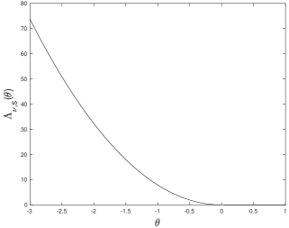
Figure 1: The function $\Lambda_{\nu,S}$ in Remark 3.1 for $\theta\leq r=1$. Numerical values: $\nu=0.5$, $\beta=0.25$; $h=0.5$ on the left, and $h=3$ on the right.

Now we present weak convergence results. In view of these results it is useful to consider the following notation:

$$\alpha(\nu):=\left\{\begin{array}[]{ll}1-\nu/2&\ \mbox{if}\ m=0\\ 1-\nu&\ \mbox{if}\ m\neq 0.\end{array}\right.$$ (7)

Proposition 3.2.

Assume that Condition 3.1 holds and let $\alpha(\nu)$ be defined in (7). We have the following statements.

• If $m=0$, then $\{t^{\alpha(\nu)}\frac{S(L_{\nu}(t))}{t}:t>0\}$ converges weakly to $\sqrt{qL_{\nu}(1)}Z$, where $Z$ is a standard Normal distributed random variable, and independent to $L_{\nu}(1)$.

• If $m\neq 0$, then $\{t^{\alpha(\nu)}\frac{S(L_{\nu}(t))}{t}:t>0\}$ converges weakly to $mL_{\nu}(1)$.

Proof.

In both cases $m=0$ and $m\neq 0$ we study suitable limits (as $t\to\infty$) in terms of the moment generating function in (6); so, when we take the limit, we have to take into account (2).

If $m=0$, then we have

$$\mathbb{E}\left[e^{\theta t^{\alpha(\nu)}\frac{S(L_{\nu}(t))}{t}}\right]=\mathbb{E}\left[e^{\theta\frac{S(L_{\nu}(t))}{t^{\nu/2}}}\right]=E_{\nu}\left(\kappa_{S}\left(\frac{\theta}{t^{\nu/2}}\right)t^{\nu}\right)\\ =E_{\nu}\left(\left(\frac{q\theta^{2}}{2t^{\nu}}+o\left(\frac{1}{t^{\nu}}\right)\right)t^{\nu}\right)\to E_{\nu}\left(\frac{q\theta^{2}}{2}\right)\ \mbox{for all}\ \theta\in\mathbb{R}.$$

Thus the desired weak convergence is proved noting that (here we take into account (3))

$$\mathbb{E}\left[e^{\theta\sqrt{qL_{\nu}(1)}Z}\right]=\mathbb{E}\left[e^{\frac{\theta^{2}q}{2}L_{\nu}(1)}\right]=E_{\nu}\left(\frac{q\theta^{2}}{2}\right)\ \mbox{for all}\ \theta\in\mathbb{R}.$$

If $m\neq 0$, then we have

$$\mathbb{E}\left[e^{\theta t^{\alpha(\nu)}\frac{S(L_{\nu}(t))}{t}}\right]=\mathbb{E}\left[e^{\theta\frac{S(L_{\nu}(t))}{t^{\nu}}}\right]=E_{\nu}\left(\kappa_{S}\left(\frac{\theta}{t^{\nu}}\right)t^{\nu}\right)\\ =E_{\nu}\left(\left(\frac{m\theta}{t^{\nu}}+o\left(\frac{1}{t^{\nu}}\right)\right)t^{\nu}\right)\to E_{\nu}\left(m\theta\right)\ \mbox{for all}\ \theta\in\mathbb{R}.$$

Thus the desired weak convergence is proved by (3). ∎

Now we present the non-central moderate deviation results.

Proposition 3.3.

Assume that Condition 3.1 holds and let $\alpha(\nu)$ be defined in (7). Moreover assume that $q>0$ if $m=0$. Then, for every family of positive numbers $\{a_{t}:t>0\}$ such that (1) holds, the family of random variables $\left\{\frac{(a_{t}t)^{\alpha(\nu)}S(L_{\nu}(t))}{t}:t>0\right\}$ satisfies the LDP with speed $1/a_{t}$ and good rate function $I_{\mathrm{MD}}(\cdot;m)$ defined by:

$$\left.\begin{array}[]{cc}\mbox{if}\ m=0,&\ I_{\mathrm{MD}}(x;0):=((\nu/2)^{\nu/(2-\nu)}-(\nu/2)^{2/(2-\nu)})\left(\frac{2x^{2}}{q}\right)^{1/(2-\nu)};\\ \mbox{if}\ m\neq 0,&\ I_{\mathrm{MD}}(x;m):=\left\{\begin{array}[]{ll}(\nu^{\nu/(1-\nu)}-\nu^{1/(1-\nu)})\left(\frac{x}{m}\right)^{1/(1-\nu)}&\ \mbox{if}\ \frac{x}{m}\geq 0\\ \infty&\ \mbox{if}\ \frac{x}{m}<0.\end{array}\right.\end{array}\right.$$

Proof.

For every $m\in\mathbb{R}$ we apply the Gärtner Ellis Theorem (Theorem 2.1). So we have to show that we can consider the function $\Lambda_{\nu,m}$ defined by

$$\Lambda_{\nu,m}(\theta):=\lim_{t\to\infty}\frac{1}{1/a_{t}}\log\mathbb{E}\left[e^{\frac{\theta}{a_{t}}\frac{(a_{t}t)^{\alpha(\nu)}S(L_{\nu}(t))}{t}}\right]\ \mbox{for all}\ \theta\in\mathbb{R},$$

or equivalently

$$\Lambda_{\nu,m}(\theta):=\lim_{t\to\infty}a_{t}\log E_{\nu}\left(\kappa_{S}\left(\frac{\theta}{(a_{t}t)^{1-\alpha(\nu)}}\right)t^{\nu}\right)\ \mbox{for all}\ \theta\in\mathbb{R};$$

in particular we refer to (2) when we take the limit. Moreover, again for every $m\in\mathbb{R}$, we shall see that the function $\Lambda_{\nu,m}$ satisfies the hypotheses of the Gärtner Ellis Theorem (this can be checked by considering the expressions of the function $\Lambda_{\nu,m}$ below), and therefore the LDP holds with good rate function $I_{\mathrm{MD}}(\cdot;m)$ defined by

$$I_{\mathrm{MD}}(x;m):=\sup_{\theta\in\mathbb{R}}\{\theta x-\Lambda_{\nu,m}(\theta)\}.$$ (8)

Then, as we shall explain below, for every $m\in\mathbb{R}$ the rate function expression in (8) coincides with the rate function $I_{\mathrm{MD}}(\cdot;m)$ in the statement.

If $m=0$ we have

$$a_{t}\log E_{\nu}\left(\kappa_{S}\left(\frac{\theta}{(a_{t}t)^{1-\alpha(\nu)}}\right)t^{\nu}\right)\\ =a_{t}\log E_{\nu}\left(\left(\frac{q\theta^{2}}{2(a_{t}t)^{\nu}}+o\left(\frac{1}{(a_{t}t)^{\nu}}\right)\right)t^{\nu}\right)=a_{t}\log E_{\nu}\left(\frac{1}{a_{t}^{\nu}}\left(\frac{q\theta^{2}}{2}+(a_{t}t)^{\nu}o\left(\frac{1}{(a_{t}t)^{\nu}}\right)\right)\right),$$

and therefore

$$\lim_{t\to\infty}a_{t}\log E_{\nu}\left(\kappa_{S}\left(\frac{\theta}{(a_{t}t)^{1-\alpha(\nu)}}\right)t^{\nu}\right)=\left(\frac{q\theta^{2}}{2}\right)^{1/\nu}=:\Lambda_{\nu,0}(\theta)\ \mbox{for all}\ \theta\in\mathbb{R};$$

thus the desired LDP holds with good rate function $I_{\mathrm{MD}}(\cdot;0)$ defined by (8) which coincides with the rate function expression in the statement (indeed one can check that, for all $x\in\mathbb{R}$, the supremum in (8) is attained at $\theta=\theta_{x}:=\left(\frac{2}{q}\right)^{1/(2-\nu)}\left(\frac{\nu x}{2}\right)^{\nu/(2-\nu)}$).

If $m\neq 0$ we have

$$a_{t}\log E_{\nu}\left(\kappa_{S}\left(\frac{\theta}{(a_{t}t)^{1-\alpha(\nu)}}\right)t^{\nu}\right)\\ =a_{t}\log E_{\nu}\left(\left(\frac{\theta m}{(a_{t}t)^{\nu}}+o\left(\frac{1}{(a_{t}t)^{\nu}}\right)\right)t^{\nu}\right)=a_{t}\log E_{\nu}\left(\frac{1}{a_{t}^{\nu}}\left(\theta m+(a_{t}t)^{\nu}o\left(\frac{1}{(a_{t}t)^{\nu}}\right)\right)\right)$$

and therefore

$$\lim_{t\to\infty}a_{t}\log E_{\nu}\left(\kappa_{S}\left(\frac{\theta}{(a_{t}t)^{1-\alpha(\nu)}}\right)t^{\nu}\right)=\left\{\begin{array}[]{ll}(\theta m)^{1/\nu}&\ \mbox{if}\ \theta m\geq 0\\ 0&\ \mbox{if}\ \theta m<0\end{array}\right.=:\Lambda_{\nu,m}(\theta)\ \mbox{for all}\ \theta\in\mathbb{R};$$

thus the desired LDP holds with good rate function $I_{\mathrm{MD}}(\cdot;m)$ defined by (8) which coincides with the rate function expression in the statement (indeed one can check that the supremum in (8) is attained at $\theta=\theta_{x}:=\frac{1}{m}\left(\frac{\nu x}{m}\right)^{\nu/(1-\nu)}$ for $\frac{x}{m}\geq 0$, and it is equal to infinity for $\frac{x}{m}<0$ by letting $\theta\to\infty$ if $m<0$, and by letting $\theta\to-\infty$ if $m>0$). ∎

Remark 3.2.

As we said above, the results in this section provide a generalization of the results in [1] in which $\{S(t):t\geq 0\}$ is a compound Poisson process. More precisely we mean that $S(t):=\sum_{k=1}^{N(t)}X_{k}$, where $\{X_{n}:n\geq 1\}$ are i.i.d. real valued light tailed random variables with finite mean $\mu$ and finite variance $\sigma^{2}$ (in [1] it was requested that $\sigma^{2}>0$ to avoid trivialities), independent of a Poisson process $\{N(t):t\geq 0\}$ with intensity $\lambda>0$. Therefore $\kappa_{S}(\theta)=\lambda(\mathbb{E}[e^{\theta X_{1}}]-1)$ for all $\theta\in\mathbb{R}$; moreover (see $m$ and $q$ in Condition 1.1) $m=\lambda\mu$ and $q=\lambda(\sigma^{2}+\mu^{2})$.

Moreover we can adapt the content of Remark 3.4 in [1] and we can say that, for every $m\in\mathbb{R}$ (thus the case $m=0$ can be also considered), we have $I_{\mathrm{MD}}(x;m)=I_{\mathrm{MD}}(-x;-m)$ for every $x\in\mathbb{R}$. Finally, if we refer to $\lambda$ and $\mu$ at the beginning of this remark, we recover the rate functions in Proposition 3.3 in [1] as follows:

• if $m=\lambda\mu=0$ (and therefore $\mu=0$ and $q=\lambda\sigma^{2}$), then $I_{\mathrm{MD}}(\cdot;0)$ in Proposition 3.3 in this paper coincides with $I_{\mathrm{MD},0}$ in Proposition 3.3 in [1];

• if $m=\lambda\mu\neq 0$ (and therefore $\mu\neq 0$), then $I_{\mathrm{MD}}(\cdot;m)$ in Proposition 3.3 in this paper coincides with $I_{\mathrm{MD},\mu}$ in Proposition 3.3 in [1].

Remark 3.3.

In Proposition 3.3 we have assumed that $q\neq 0$ when $m=0$. Indeed, if $q=0$ and $m=0$, the process $\{S(L_{\nu}(t)):t\geq 0\}$ in Propositions 3.1, 3.2 and 3.3 is identically equal to zero (because $S(t)=0$ for all $t\geq 0$) and the weak convergence in Proposition 3.2 (for $m=0$) is towards a constant random variable (i.e. the costant random variable equal to zero). Moreover, again if $q=0$ and $m=0$, the rate function $I_{\mathrm{MD}}(x;0)$ in Proposition 3.3 is not well-defined (because there is a denominator equal to zero).

4 Results with two independent random time-changes

Throughout this section we assume that the following condition holds.

Condition 4.1.

Let $\{S(t):t\geq 0\}$ be a real-valued Lévy process as in Condition 1.1, and let $\{L_{\nu_{1}}^{(1)}(t):t\geq 0\}$ and $\{L_{\nu_{2}}^{(2)}(t):t\geq 0\}$ be two independent inverses of stable subordinators for $\nu_{1},\nu_{2}\in(0,1)$, and independent of $\{S(t):t\geq 0\}$. We assume that $\{S(t):t\geq 0\}$ has bounded variation, and it is not a subordinator.

We have the following consequence of Condition 4.1.

Lemma 4.1.

Assume that Condition 4.1 holds. Then there exists two non-null independent subordinators $\{S_{1}(t):t\geq 0\}$ and $\{S_{2}(t):t\geq 0\}$ such that $\{S(t):t\geq 0\}$ is distributed as $\{S_{1}(t)-S_{2}(t):t\geq 0\}$.

We can assume that the statement in Lemma 4.1 is known even if we do not have an exact reference for that result (however a statement of this kind appears in the Introduction of [2]). The idea of the proof is the following. If $\Pi(dx)$ is the Lévy measure of a Lévy process with bounded variation, then $1_{(0,\infty)}(x)\Pi(dx)$ and $1_{(-\infty,0)}(x)\Pi(dx)$ are again Lévy measures of Lévy processes with bounded variation; thus $1_{(0,\infty)}(x)\Pi(dx)$ is the Lévy measure associated to the subordinator $\{S_{1}(t):t\geq 0\}$, $1_{(-\infty,0)}(x)\Pi(dx)$ is the Lévy measure associated to the opposite of the subordinator $\{S_{2}(t):t\geq 0\}$, and $\{S_{1}(t):t\geq 0\}$ and $\{S_{2}(t):t\geq 0\}$ are independent.

Remark 4.1.

Let $\kappa_{S_{1}}$ and $\kappa_{S_{2}}$ be the analogue of the function $\kappa_{S}$ for the process $\{S(t):t\geq 0\}$ in Condition 1.1, i.e. the functions defined by

$$\kappa_{S_{i}}(\theta):=\log\mathbb{E}[e^{\theta S_{i}(1)}]\quad(\mbox{for}\ i=1,2),$$

where $\{S_{1}(t):t\geq 0\}$ and $\{S_{2}(t):t\geq 0\}$ are the subordinators in Lemma 4.1. In particular both functions are finite in a neighborhood of the origin. Then, if we set

$$m_{i}=\kappa_{S_{i}}^{\prime}(0)\quad\mbox{and}\quad q_{i}=\kappa_{S_{i}}^{\prime\prime}(0)\quad(\mbox{for}\ i\in\{1,2\}),$$

we have (we recall that $\kappa_{S}(\theta)=\kappa_{S_{1}}(\theta)+\kappa_{S_{2}}(-\theta)$ for all $\theta\in\mathbb{R}$)

$$m=\kappa_{S}^{\prime}(0)=m_{1}-m_{2}\quad\mbox{and}\quad q=\kappa_{S}^{\prime\prime}(0)=q_{1}+q_{2}.$$

We recall that, since $\{S_{1}(t):t\geq 0\}$ and $\{S_{2}(t):t\geq 0\}$ are non-trivial subordinators, then $m_{1},m_{2}>0$.

The next Propositions 4.1, 4.2 and 4.3 provide a generalization of Propositions 3.1, 3.2 and 3.3 in [7], respectively, in which $\{S(t):t\geq 0\}$ is a Skellam process (and therefore $\{S_{1}(t):t\geq 0\}$ and $\{S_{2}(t):t\geq 0\}$ are two Poisson processes with intensities $\lambda_{1}$ and $\lambda_{2}$, respectively). We start with the reference LDP for the convergence in probability to zero of $\left\{\frac{S_{1}(L_{\nu_{1}}^{(1)}(t))-S_{2}(L_{\nu_{2}}^{(2)}(t))}{t}:t>0\right\}$. In this first result the case $\nu_{1}\neq\nu_{2}$ is allowed.

Proposition 4.1.

Assume that Condition 4.1 holds. Let $\Psi_{\nu_{1},\nu_{2}}$ be the function defined by

$$\Psi_{\nu_{1},\nu_{2}}(\theta):=\left\{\begin{array}[]{ll}(\kappa_{S_{1}}(\theta))^{1/\nu_{1}}&\ \mbox{if}\ \theta\geq 0\\ (\kappa_{S_{2}}(-\theta))^{1/\nu_{2}}&\ \mbox{if}\ \theta<0.\end{array}\right.$$ (9)

Then $\left\{\frac{S_{1}(L_{\nu_{1}}^{(1)}(t))-S_{2}(L_{\nu_{2}}^{(2)}(t))}{t}:t>0\right\}$ satisfies the LDP with speed $v_{t}=t$ and good rate function $J_{\mathrm{LD}}$ defined by

$$J_{\mathrm{LD}}(x):=\sup_{\theta\in\mathbb{R}}\{\theta x-\Psi_{\nu_{1},\nu_{2}}(\theta)\}.$$ (10)

Proof.

We prove this proposition by applying the Gärtner Ellis Theorem. More precisely we have to show that

$$\lim_{t\to\infty}\frac{1}{t}\log\mathbb{E}\left[e^{t\theta\frac{S_{1}(L_{\nu_{1}}^{(1)}(t))-S_{2}(L_{\nu_{2}}^{(2)}(t))}{t}}\right]=\Psi_{\nu_{1},\nu_{2}}(\theta)\ (\mbox{for all}\ \theta\in\mathbb{R}),$$ (11)

where $\Psi_{\nu_{1},\nu_{2}}$ is the function in (9).

The case $\theta=0$ is immediate. For $\theta\neq 0$ we have

$$\log\mathbb{E}\left[e^{t\theta\frac{S_{1}(L_{\nu_{1}}^{(1)}(t))-S_{2}(L_{\nu_{2}}^{(2)}(t))}{t}}\right]=\log E_{\nu_{1}}(\kappa_{S_{1}}(\theta)t^{\nu_{1}})+\log E_{\nu_{2}}(\kappa_{S_{2}}(-\theta)t^{\nu_{2}}).$$

Then, by taking into account the asymptotic behaviour of the Mittag-Leffler function in (2), we have

$$\lim_{t\to\infty}\frac{1}{t}\log E_{\nu_{1}}(\kappa_{S_{1}}(\theta)t^{\nu_{1}})+\lim_{t\to\infty}\frac{1}{t}\log E_{\nu_{2}}(\kappa_{S_{2}}(-\theta)t^{\nu_{2}})=(\kappa_{S_{1}}(\theta))^{1/\nu_{1}}\ \mbox{for}\ \theta>0,$$

and

$$\lim_{t\to\infty}\frac{1}{t}\log E_{\nu_{1}}(\kappa_{S_{1}}(\theta)t^{\nu_{1}})+\lim_{t\to\infty}\frac{1}{t}\log E_{\nu_{2}}(\kappa_{S_{2}}(-\theta)t^{\nu_{2}})=(\kappa_{S_{2}}(-\theta))^{1/\nu_{2}}\ \mbox{for}\ \theta<0;$$

thus the limit in (11) is checked. Finally the desired LDP holds because the function $\Psi_{\nu_{1},\nu_{2}}$ is essentially smooth. The essential smoothness of $\Psi_{\nu_{1},\nu_{2}}$ trivially holds if $\Psi_{\nu_{1},\nu_{2}}(\theta)$ is finite everywhere (and differentiable). So now we assume that $\Psi_{\nu_{1},\nu_{2}}(\theta)$ is not finite everywhere. For $i=1,2$ we have

$$\frac{d}{d\theta}(\kappa_{S_{i}}(\theta))^{1/\nu_{i}}=\frac{1}{\nu_{i}}(\kappa_{S_{i}}(\theta))^{1/\nu_{i}-1}\kappa_{S_{i}}^{\prime}(\theta),$$

and therefore the range of values of each one of these derivatives (for $\theta\geq 0$ such that $\kappa_{S_{i}}(\theta)<\infty$) is $[0,\infty)$; therefore the range of values of $\Psi_{\nu_{1},\nu_{2}}^{\prime}(\theta)$ (for $\theta\in\mathbb{R}$ such that $\Psi_{\nu_{1},\nu_{2}}(\theta)<\infty$) is $(-\infty,\infty)$, and the essential smoothness of $\Psi_{\nu_{1},\nu_{2}}$ is proved. ∎

From now on we assume that $\nu_{1}$ and $\nu_{2}$ coincide, and therefore we simply consider the symbol $\nu$, where $\nu=\nu_{1}=\nu_{2}$. Moreover we set

$$\alpha_{1}(\nu):=1-\nu.$$ (12)

Proposition 4.2.

Assume that Condition 4.1 holds. Moreover assume that $\nu_{1}=\nu_{2}=\nu$ for some $\nu\in(0,1)$ and let $\alpha_{1}(\nu)$ be defined in (12). Then $\{t^{\alpha_{1}(\nu)}\frac{S_{1}(L_{\nu}^{(1)}(t))-S_{2}(L_{\nu}^{(2)}(t))}{t}:t>0\}$ converges weakly to $m_{1}L_{\nu}^{(1)}(1)-m_{2}L_{\nu}^{(2)}(1)$.

Proof.

We have to check that

$$\lim_{t\to\infty}\mathbb{E}\left[e^{\theta t^{\alpha_{1}(\nu)}\frac{S_{1}(L_{\nu}^{(1)}(t))-S_{2}(L_{\nu}^{(2)}(t))}{t}}\right]=\underbrace{\mathbb{E}\left[e^{\theta(m_{1}L_{\nu}^{(1)}(1)-m_{2}L_{\nu}^{(2)}(1))}\right]}_{=E_{\nu}(m_{1}\theta)E_{\nu}(-m_{2}\theta)}\ (\mbox{for all}\ \theta\in\mathbb{R})$$

(here we take into account that $L_{\nu}^{(1)}(1)$ and $L_{\nu}^{(2)}(1)$ are i.i.d., and the expression of the moment generating function in (3)). This can be readily done noting that

$$\mathbb{E}\left[e^{\theta t^{\alpha_{1}(\nu)}\frac{S_{1}(L_{\nu}^{(1)}(t))-S_{2}(L_{\nu}^{(2)}(t))}{t}}\right]=\mathbb{E}\left[e^{\theta\frac{S_{1}(L_{\nu}^{(1)}(t))-S_{2}(L_{\nu}^{(2)}(t))}{t^{\nu}}}\right]\\ =E_{\nu}\left(\kappa_{S_{1}}\left(\frac{\theta}{t^{\nu}}\right)t^{\nu}\right)E_{\nu}\left(\kappa_{S_{2}}\left(-\frac{\theta}{t^{\nu}}\right)t^{\nu}\right)\\ =E_{\nu}\left(\left(m_{1}\frac{\theta}{t^{\nu}}+o\left(\frac{1}{t^{\nu}}\right)\right)t^{\nu}\right)E_{\nu}\left(\left(-m_{2}\frac{\theta}{t^{\nu}}+o\left(\frac{1}{t^{\nu}}\right)t^{\nu}\right)\right),$$

and we get the desired limit letting $t$ go to infinity (for each fixed $\theta\in\mathbb{R}$). ∎

Proposition 4.3.

Assume that Condition 4.1 holds. Moreover assume that $\nu_{1}=\nu_{2}=\nu$ for some $\nu\in(0,1)$ and let $\alpha_{1}(\nu)$ be defined in (12). Then, for every family of positive numbers $\{a_{t}:t>0\}$ such that (1) holds, the family of random variables $\left\{(a_{t}t)^{\alpha_{1}(\nu)}\frac{S_{1}(L_{\nu}^{(1)}(t))-S_{2}(L_{\nu}^{(2)}(t))}{t}:t>0\right\}$ satisfies the LDP with speed $1/a_{t}$ and good rate function $J_{\mathrm{MD}}$ defined by

$$J_{\mathrm{MD}}(x):=\left\{\begin{array}[]{ll}(\nu^{\nu/(1-\nu)}-\nu^{1/(1-\nu)})\left(\frac{x}{m_{1}}\right)^{1/(1-\nu)}&\ \mbox{if}\ x\geq 0\\ (\nu^{\nu/(1-\nu)}-\nu^{1/(1-\nu)})\left(-\frac{x}{m_{2}}\right)^{1/(1-\nu)}&\ \mbox{if}\ x<0.\end{array}\right.$$

Proof.

We prove this proposition by applying the Gärtner Ellis Theorem. More precisely we have to show that

$$\lim_{t\to\infty}\frac{1}{1/a_{t}}\log\mathbb{E}\left[e^{\frac{\theta}{a_{t}}(a_{t}t)^{\alpha_{1}(\nu)}\frac{S_{1}(L_{\nu}^{(1)}(t))-S_{2}(L_{\nu}^{(2)}(t))}{t}}\right]=\widetilde{\Psi}_{\nu}(\theta)\ (\mbox{for all}\ \theta\in\mathbb{R}),$$ (13)

where $\widetilde{\Psi}_{\nu}$ is the function defined by

$$\widetilde{\Psi}_{\nu}(\theta):=\left\{\begin{array}[]{ll}(m_{1}\theta)^{1/\nu}&\ \mbox{if}\ \theta\geq 0\\ (-m_{2}\theta)^{1/\nu}&\ \mbox{if}\ \theta<0;\end{array}\right.$$

indeed, since the function $\widetilde{\Psi}_{\nu}$ is finite (for all $\theta\in\mathbb{R}$) and differentiable, the desired LDP holds noting that the Legendre-Fenchel transform $\widetilde{\Psi}_{\nu}^{*}$ of $\widetilde{\Psi}_{\nu}$, i.e. the function $\widetilde{\Psi}_{\nu}^{*}$ defined by

$$\widetilde{\Psi}_{\nu}^{*}(x):=\sup_{\theta\in\mathbb{R}}\{\theta x-\widetilde{\Psi}_{\nu}(\theta)\}\ (\mbox{for all}\ x\in\mathbb{R}),$$ (14)

coincides with the function $J_{\mathrm{MD}}$ in the statement of the proposition (for $x=0$ the supremum in (14) is attained at $\theta=0$, for $x>0$ that supremum is attained at $\theta=\frac{1}{m_{1}}(\frac{\nu x}{m_{1}})^{\nu/(1-\nu)}$, for $x<0$ that supremum is attained at $\theta=-\frac{1}{m_{2}}(-\frac{\nu x}{m_{2}})^{\nu/(1-\nu)}$).

So we conclude the proof by checking the limit in (13). The case $\theta=0$ is immediate. For $\theta\neq 0$ we have

$$\log\mathbb{E}\left[e^{\frac{\theta}{a_{t}}(a_{t}t)^{\alpha_{1}(\nu)}\frac{S_{1}(L_{\nu}^{(1)}(t))-S_{2}(L_{\nu}^{(2)}(t))}{t}}\right]=\log\mathbb{E}\left[e^{\theta\frac{S_{1}(L_{\nu}^{(1)}(t))-S_{2}(L_{\nu}^{(2)}(t))}{(a_{t}t)^{\nu}}}\right]\\ =\log E_{\nu}\left(\kappa_{S_{1}}\left(\frac{\theta}{(a_{t}t)^{\nu}}\right)t^{\nu}\right)+\log E_{\nu}\left(\kappa_{S_{2}}\left(-\frac{\theta}{(a_{t}t)^{\nu}}\right)t^{\nu}\right)\\ =\log E_{\nu}\left(\left(m_{1}\frac{\theta}{(a_{t}t)^{\nu}}+o\left(\frac{1}{(a_{t}t)^{\nu}}\right)\right)t^{\nu}\right)+\log E_{\nu}\left(\left(-m_{2}\frac{\theta}{(a_{t}t)^{\nu}}+o\left(\frac{1}{(a_{t}t)^{\nu}}\right)\right)t^{\nu}\right)\\ =\log E_{\nu}\left(\frac{m_{1}}{a_{t}^{\nu}}\left(\theta+(a_{t}t)^{\nu}o\left(\frac{1}{(a_{t}t)^{\nu}}\right)\right)\right)+\log E_{\nu}\left(\frac{m_{2}}{a_{t}^{\nu}}\left(-\theta+(a_{t}t)^{\nu}o\left(\frac{1}{(a_{t}t)^{\nu}}\right)\right)\right).$$

Then, by taking into account the asymptotic behaviour of the Mittag-Leffler function in (2), we have

$$\lim_{t\to\infty}\frac{1}{1/a_{t}}\log\mathbb{E}\left[e^{\frac{\theta}{a_{t}}(a_{t}t)^{\alpha_{1}(\nu)}\frac{S_{1}(L_{\nu}^{(1)}(t))-S_{2}(L_{\nu}^{(2)}(t))}{t}}\right]=(m_{1}\theta)^{1/\nu}\quad\mbox{for}\ \theta>0,$$

and

$$\lim_{t\to\infty}\frac{1}{1/a_{t}}\log\mathbb{E}\left[e^{\frac{\theta}{a_{t}}(a_{t}t)^{\alpha_{1}(\nu)}\frac{S_{1}(L_{\nu}^{(1)}(t))-S_{2}(L_{\nu}^{(2)}(t))}{t}}\right]=(-m_{2}\theta)^{1/\nu}\quad\mbox{for}\ \theta<0.$$

Thus the limit in (13) is checked. ∎

5 Comparisons between rate functions

In this section $\{S(t):t\geq 0\}$ is a real-valued Lévy process as in Condition 1.1, with bounded variation, and it is not a subordinator; thus we can refer to both Conditions 3.1 and 4.1, and in particular (as stated in Lemma 4.1) we can refer to the non-trivial independent subordinators $\{S_{1}(t):t\geq 0\}$ and $\{S_{2}(t):t\geq 0\}$ such that $\{S(t):t\geq 0\}$ is distributed as $\{S_{1}(t)-S_{2}(t):t\geq 0\}$. In particular we can refer to the LDPs in Propositions 3.1 and 4.1, which are governed by the rate functions $I_{\mathrm{LD}}$ and $J_{\mathrm{LD}}$, and to the classes of LDPs in Propositions 3.3 and 4.3, which are governed by the rate functions $I_{\mathrm{MD}}(\cdot;m)=I_{\mathrm{MD}}(\cdot;m_{1}-m_{2})$ and $J_{\mathrm{MD}}$. All these rate functions uniquely vanish at $x=0$. So, by arguing as in [7] (Section 5), we present some generalizations of the comparisons between rate functions (at least around $x=0$) presented in that reference. Those comparisons allow to compare different convergences to zero; this could be explained by adapting the explanations in [7] (Section 5), and here we omit the details.

Remark 5.1.

Throughout this section we always assume that $\nu_{1}=\nu_{2}=\nu$ for some $\nu\in(0,1)$. So we simply write $\Psi_{\nu}$ in place of the function $\Psi_{\nu_{1},\nu_{2}}$ in Proposition 4.1 (see (9)).

We start by comparing $J_{\mathrm{LD}}$ in Proposition 4.1 and $I_{\mathrm{LD}}$ in Proposition 3.1.

Proposition 5.1.

Assume that $\nu_{1}=\nu_{2}=\nu$ for some $\nu\in(0,1)$. Then $J_{\mathrm{LD}}(0)=I_{\mathrm{LD}}(0)=0$ and, for $x\neq 0$, we have $I_{\mathrm{LD}}(x)>J_{\mathrm{LD}}(x)>0$.

Proof.

Firstly, since the range of values of $\Psi_{\nu}^{\prime}(\theta)$ (for $\theta$ such that the derivative is well-defined) is $(-\infty,\infty)$ (see the final part of the proof of Proposition 4.1, and the change of notation in Remark 5.1), for all $x\in\mathbb{R}$ there exists $\theta_{x}^{(1)}$ such that $\Psi_{\nu}^{\prime}(\theta_{x}^{(1)})=x$, and therefore

$$J_{\mathrm{LD}}(x)=\theta_{x}^{(1)}x-\Psi_{\nu}(\theta_{x}^{(1)}).$$

We recall that $\theta_{x}^{(1)}=0$ ($\theta_{x}^{(1)}>0$ and $\theta_{x}^{(1)}<0$, respectively) if and only if $x=0$ ($x>0$ and $x<0$, respectively). Then $J_{\mathrm{LD}}(0)=0$ and, moreover, we have $I_{\mathrm{LD}}(0)=0$; indeed the equation $\Lambda_{\nu,S}^{\prime}(\theta)=0$, i.e.

$$\frac{1}{\nu}(\kappa_{S_{1}}(\theta)+\kappa_{S_{2}}(-\theta))^{1/\nu-1}(\kappa_{S_{1}}^{\prime}(\theta)+\kappa_{S_{2}}^{\prime}(-\theta))=0,$$

yields the solution $\theta=0$.

We conclude with the case $x\neq 0$. If $x>0$, then we have

$$\kappa_{S_{1}}(\theta_{x}^{(1)})>\max\{\kappa_{S_{1}}(\theta_{x}^{(1)})+\kappa_{S_{2}}(-\theta_{x}^{(1)}),0\};$$

this yields $\Psi_{\nu}(\theta_{x}^{(1)})>\Lambda_{\nu,S}(\theta_{x}^{(1)})$, and therefore

$$J_{\mathrm{LD}}(x)=\theta_{x}^{(1)}x-\Psi_{\nu}(\theta_{x}^{(1)})<\theta_{x}^{(1)}x-\Lambda_{\nu,S}(\theta_{x}^{(1)})\leq\sup_{\theta\in\mathbb{R}}\{\theta x-\Lambda_{\nu,S}(\theta)\}=I_{\mathrm{LD}}(x).$$

Similarly, if $x<0$, then we have

$$\kappa_{S_{2}}(-\theta_{x}^{(1)})>\max\{\kappa_{S_{1}}(\theta_{x}^{(1)})+\kappa_{S_{2}}(-\theta_{x}^{(1)}),0\};$$

this yields $\Psi_{\nu}(\theta_{x}^{(1)})>\Lambda_{\nu,S}(\theta_{x}^{(1)})$, and we can conclude following the lines of of the case $x>0$. ∎

The next Proposition 5.2 provides a similar result which concerns the comparison of $J_{\mathrm{MD}}$ in Proposition 4.3 and $I_{\mathrm{MD}}(\cdot;m)=I_{\mathrm{MD}}(\cdot;m_{1}-m_{2})$ in Proposition 3.3. In particular we have $I_{\mathrm{MD}}(x;m_{1}-m_{2})>J_{\mathrm{MD}}(x)>0$ for all $x\neq 0$ if and only if $m_{1}\neq m_{2}$ (note that, if $m_{1}\neq m_{2}$, we have $m=m_{1}-m_{2}\neq 0$; thus $\alpha(\nu)$ in (7) coincides with $\alpha_{1}(\nu)$ in (12)); on the contrary, if $m_{1}=m_{2}$, we have $I_{\mathrm{MD}}(x;0)>J_{\mathrm{MD}}(x)>0$ only if $|x|$ is small enough (and strictly positive).

Proposition 5.2.

We have $J_{\mathrm{MD}}(0)=I_{\mathrm{MD}}(0;m_{1}-m_{2})=0$. Moreover, if $x\neq 0$, we have two cases.

1. If $m_{1}\neq m_{2}$, then $I_{\mathrm{MD}}(x;m_{1}-m_{2})>J_{\mathrm{MD}}(x)>0$.

2. If $m_{1}=m_{2}=m_{*}$ for some $m_{*}>0$, there exists $\delta_{\nu}>0$ such that: $I_{\mathrm{MD}}(x;0)>J_{\mathrm{MD}}(x)>0$ if $0<|x|<\delta_{\nu}$, $J_{\mathrm{MD}}(x)>I_{\mathrm{MD}}(x;0)>0$ if $|x|>\delta_{\nu}$, and $I_{\mathrm{MD}}(x;0)=J_{\mathrm{MD}}(x)>0$ if $|x|=\delta_{\nu}$.

Proof.

The equality $J_{\mathrm{MD}}(0)=I_{\mathrm{MD}}(0;m_{1}-m_{2})=0$ (case $x=0$) is immediate. So, in what follows, we take $x\neq 0$. We start with the case $m_{1}\neq m_{2}$, and we have two cases.

• Assume that $m_{1}>m_{2}$. Then for $x<0$ we have $J_{\mathrm{MD}}(x)<\infty=I_{\mathrm{MD}}(x;m_{1}-m_{2})$. For $x>0$ we have $\frac{x}{m_{1}}<\frac{x}{m_{1}-m_{2}}$, which is trivially equivalent to $J_{\mathrm{MD}}(x)<I_{\mathrm{MD}}(x;m_{1}-m_{2})$.

• Assume that $m_{1}<m_{2}$. Then for $x>0$ we have $J_{\mathrm{MD}}(x)<\infty=I_{\mathrm{MD}}(x;m_{1}-m_{2})$. For $x<0$ we have $-\frac{x}{m_{2}}<-\frac{x}{m_{2}-m_{1}}$, which is trivially equivalent to $J_{\mathrm{MD}}(x)<I_{\mathrm{MD}}(x;m_{1}-m_{2})$.

Finally, if $m_{1}=m_{2}=m_{*}$ for some $m_{*}>0$, the statement to prove trivially holds noting that, for two constants $c_{\nu,m_{*}}^{(1)},c_{\nu,m_{*}}^{(2)}>0$, we have $J_{\mathrm{MD}}(x)=c_{\nu,m_{*}}^{(1)}|x|^{1/(1-\nu)}$ and $I_{\mathrm{MD}}(x;0)=c_{\nu,m_{*}}^{(2)}|x|^{1/(1-\nu/2)}$. ∎

We remark that the inequalities around $x=0$ in Propositions 5.1 and 5.2 are not surprising; indeed we expect to have a slower convergence to zero when we deal with two independent random time-changes (because in that case we have more randomness).

Now we consider comparisons between rate functions for different values of $\nu\in(0,1)$. We mean the rate functions in Propositions 3.1 and 4.1, and we restrict our attention to a comparison around $x=0$. In view of what follows, we consider some slightly different notation: $I_{\mathrm{LD},\nu}$ in place of $I_{\mathrm{LD}}$ in Proposition 3.1; $J_{\mathrm{LD},\nu}$ in place of $J_{\mathrm{LD}}$ in Proposition 4.1, with $\nu_{1}=\nu_{2}=\nu$ for some $\nu\in(0,1)$.

Proposition 5.3.

Let $\nu,\eta\in(0,1)$ be such that $\eta<\nu$. Then: $I_{\mathrm{LD},\eta}(0)=I_{\mathrm{LD},\nu}(0)=0$, $J_{\mathrm{LD},\eta}(0)=J_{\mathrm{LD},\nu}(0)=0$; for some $\delta>0$, we have $I_{\mathrm{LD},\eta}(x)>I_{\mathrm{LD},\nu}(x)>0$ and $J_{\mathrm{LD},\eta}(x)>J_{\mathrm{LD},\nu}(x)>0$ for $0<|x|<\delta$.

Proof.

We can say that there exists $\delta>0$ small enough such that, for $|x|<\delta$, there exist $\theta_{x,\nu}^{(1)},\theta_{x,\nu}^{(2)}\in\mathbb{R}$ such that:

$$I_{\mathrm{LD},\nu}(x)=\theta_{x,\nu}^{(2)}x-\Lambda_{\nu,S}(\theta_{x,\nu}^{(2)})\ \mbox{and}\ J_{\mathrm{LD},\nu}(x)=\theta_{x,\nu}^{(1)}x-\Psi_{\nu}(\theta_{x,\nu}^{(1)});$$

moreover $\theta_{x,\nu}^{(1)}=\theta_{x,\nu}^{(2)}=0$ if $x=0$, and $\theta_{x,\nu}^{(1)},\theta_{x,\nu}^{(2)}\neq 0$ if $x\neq 0$; finally we have

$$0\leq\Psi_{\nu}(\theta_{x,\nu}^{(1)}),\Lambda_{\nu,S}(\theta_{x,\nu}^{(2)})<1.$$

Then, by taking into account the same formulas with $\eta$ in place of $\nu$ (together with the inequality $\frac{1}{\eta}>\frac{1}{\nu}$), it is easy to check that

$$0\leq\Lambda_{\eta,S}(\theta_{x,\nu}^{(2)})<\Lambda_{\nu,S}(\theta_{x,\nu}^{(2)})<1\quad\mbox{and}\quad 0\leq\Psi_{\eta}(\theta_{x,\nu}^{(1)})<\Psi_{\nu}(\theta_{x,\nu}^{(1)})<1$$

(see (4) for the first chain of inequalities, and (9) with $\nu_{1}=\nu_{2}=\nu$ for the second chain of inequalities); thus

$$I_{\mathrm{LD},\nu}(x)=\theta_{x,\nu}^{(2)}x-\Lambda_{\nu,S}(\theta_{x,\nu}^{(2)})<\theta_{x,\nu}^{(2)}x-\Lambda_{\eta,S}(\theta_{x,\nu}^{(2)})\leq\sup_{\theta\in\mathbb{R}}\{\theta x-\Lambda_{\eta,S}(\theta)\}=I_{\mathrm{LD},\eta}(x)$$

and

$$J_{\mathrm{LD},\nu}(x)=\theta_{x,\nu}^{(1)}x-\Psi_{\nu}(\theta_{x,\nu}^{(1)})<\theta_{x,\nu}^{(1)}x-\Psi_{\eta}(\theta_{x,\nu}^{(1)})\leq\sup_{\theta\in\mathbb{R}}\{\theta x-\Psi_{\eta}(\theta)\}=J_{\mathrm{LD},\eta}(x).$$

This completes the proof. ∎

As a consequence of Proposition 5.3 we can say, in all the above convergences to zero governed by some rate function (that uniquely vanishes at zero), the smaller the $\nu$, the faster the convergence of the random variables to zero.

We also remark that we can obtain a version of Proposition 5.3 in terms of the rate functions $I_{\mathrm{MD}}(\cdot;m_{1}-m_{2})=I_{\mathrm{MD},\nu}(\cdot;m_{1}-m_{2})$ in Proposition 3.3 and $J_{\mathrm{MD}}=J_{\mathrm{MD},\nu}$ in Proposition 4.3. Indeed we can obtain the same kind of inequalities, and this is easy to check because we have explicit expressions of the rate functions (here we omit the details).

6 An example with independent tempered stable subordinators

Throughout this section we consider the examples presented below.

Example 6.1.

Let $\{S_{1}(t):t\geq 0\}$ and $\{S_{2}(t):t\geq 0\}$ be two independent tempered stable subordinators with parameters $\beta\in(0,1)$ and $r_{1}>0$, and $\beta\in(0,1)$ and $r_{2}>0$, respectively. Then

$$\kappa_{S_{i}}(\theta):=\left\{\begin{array}[]{ll}r_{i}^{\beta}-(r_{i}-\theta)^{\beta}&\ \mbox{if}\ \theta\leq r_{i}\\ \infty&\ \mbox{if}\ \theta>r_{i}\end{array}\right.$$

for $i=1,2$; thus

$$\kappa_{S}(\theta):=\kappa_{S_{1}}(\theta)+\kappa_{S_{2}}(-\theta)=\left\{\begin{array}[]{ll}r_{1}^{\beta}-(r_{1}-\theta)^{\beta}+r_{2}^{\beta}-(r_{2}+\theta)^{\beta}&\ \mbox{if}\ -r_{2}\leq\theta\leq r_{1}\\ \infty&\ \mbox{otherwise}.\end{array}\right.$$

Note that, in order to be consistent in the comparisons between $I_{\mathrm{LD}}$ and $J_{\mathrm{LD}}$, we always take the rate function $J_{\mathrm{LD}}$ in Proposition 4.1 with $\nu_{1}=\nu_{2}=\nu$. Moreover, we remark that, for Example 6.1, the function $\Lambda_{\nu,S}$ is essentially smooth because

$$\lim_{\theta\downarrow-r_{2}}\Lambda_{\nu,S}^{\prime}(\theta)=-\infty\quad\mbox{and}\quad\lim_{\theta\uparrow r_{1}}\Lambda_{\nu,S}^{\prime}(\theta)=+\infty;$$

indeed these conditions holds if and only if $\kappa_{S}(r_{1})$ and $\kappa_{S}(-r_{2})$ are positive, and in fact we have

$$\kappa_{S}(r_{1})=\kappa_{S}(-r_{2})=r_{1}^{\beta}+r_{2}^{\beta}-(r_{1}+r_{2})^{\beta}=(r_{1}+r_{2})^{\beta}\left(\left(\frac{r_{1}}{r_{1}+r_{2}}\right)^{\beta}+\left(\frac{r_{2}}{r_{1}+r_{2}}\right)^{\beta}-1\right)>0.$$

We start with Figure 2. The graphs agree with the inequalities in Proposition 5.3. Moreover Figure 2 is more informative than Figure 3 in [7]; indeed the graphs of $J_{\mathrm{LD}}=J_{\mathrm{LD},\nu}$ on the right (for different values of $\nu$) show that the inequalities in Proposition 5.3 hold only in a neighborhood of the origin $x=0$.

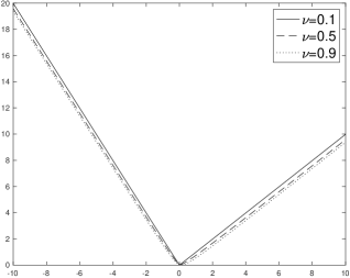
Figure 2: Rate functions $I_{\mathrm{LD}}=I_{\mathrm{LD},\nu}$ (on the left) and $J_{\mathrm{LD}}=J_{\mathrm{LD},\nu}$ (on the right) for the processes in Example 6.1 and different values of $\nu$ ($\nu=0.1,0.5,0.9$). Numerical values of the other parameters: $r_{1}=1$, $r_{2}=2$, $\beta=0.5$.

In the next Figures 3 and 4 we take different values of $\beta$ and of $r_{2}$, respectively, when the other paramaters are fixed. The graphs in these figures agree with Proposition 5.1.

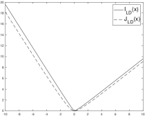
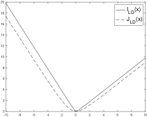
Figure 3: Rate functions $I_{\mathrm{LD}}$ and $J_{\mathrm{LD}}$ for the processes in Example 6.1 and different values of $\beta$ ($\beta=0.3,0.5,0.7$ from left to right). Numerical values of the other parameters: $r_{1}=1$, $r_{2}=2$, $\nu=0.5$.

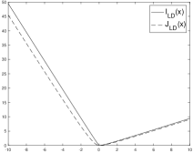
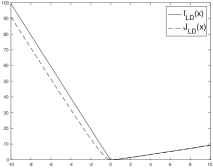
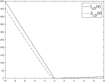
Figure 4: Rate functions $I_{\mathrm{LD}}$ and $J_{\mathrm{LD}}$ for the processes in Example 6.1 and different values of $r_{2}$ ($r_{2}=5,10,50$ from left to right). Numerical values of the other parameters: $r_{1}=1$, $\nu=0.5$, $\beta=0.5$.

Funding.

A.I. acknowledges the support of MUR-PRIN 2022 PNRR (project P2022XSF5H “Stochastic Models in Biomathematics and Applications”) and by INdAM-GNCS.
C.M. acknowledges the support of MUR Excellence Department Project awarded to the Department of Mathematics, University of Rome Tor Vergata (CUP E83C23000330006), by University of Rome Tor Vergata (project ”Asymptotic Properties in Probability” (CUP E83C22001780005)) and by INdAM-GNAMPA.
A.M. acknowledges the support of MUR-PRIN 2022 (project 2022XZSAFN “Anomalous Phenomena on Regular and Irregular Domains: Approximating Complexity for the Applied Sciences”), by MUR-PRIN 2022 PNRR (project P2022XSF5H “Stochastic Models in Biomathematics and Applications”) and by INdAM-GNCS.

References

- [1] L. Beghin, C. Macci (2022) Non-central moderate deviations for compound fractional Poisson processes. Statist. Probab. Lett. 185, Paper No. 109424, 8 pp. (2022).
- [2] Z. Chi (2016) On exact sampling of the first passage event of a Lévy process with infinite Lévy measure and bounded variation. Stochastic Processes Appl. 126, 1124–1144.
- [3] A. Dembo, O. Zeitouni (1998) Large Deviations Techniques and Applications (Second Edition). Springer-Verlag, New York.
- [4] R. Giuliano, C. Macci (2023) Some examples of noncentral moderate deviations for sequences of real random variables. Mod. Stoch. Theory Appl. 10, 111–144.
- [5] R. Gorenflo, A.A. Kilbas, F. Mainardi, S.V. Rogosin (2014) Mittag-Leffler Functions, Related Topics and Applications. Springer, New York.
- [6] A. Kerss, N.N. Leonenko, A. Sikorskii (2014) Fractional Skellam processes with applications to finance. Fract. Calc. Appl. Anal. 17, 532–551.
- [7] J. Lee, C. Macci (2024+) Noncentral moderate deviations for fractional Skellam processes. Mod. Stoch. Theory Appl., to appear.
- [8] M.M. Meerschaert, E. Nane, P. Vellaisamy (2011) The fractional Poisson process and the inverse stable subordinator. Electron. J. Probab. 16, 1600–1620.
- [9] M.M. Meerschaert, A. Sikorskii (2012) Stochastic models for fractional calculus. de Gruyter, Berlin.