Abstract

In this paper, we conduct a comprehensive exploration of the relativistic quantum dynamics of spin-0 scalar particles, as described by the Duffin-Kemmer-Petiau (DKP) equation, within the framework of a magnetic space-time. Our focus is on the Bonnor-Melvin-Lambda (BML) solution, a four-dimensional magnetic universe characterized by a magnetic field that varies with axial distance. To initiate this investigation, we derive the radial equation using a suitable wave function ansatz and subsequently employ special functions to solve it. Furthermore, we extend our analysis to include Duffin-Kemmer-Petiau oscillator fields within the same BML space-time background. We derive the corresponding radial equation and solve it using special functions. Significantly, our results show that the geometry’s topology and the cosmological constant (both are related with the magnetic field strength) influences the eigenvalue solution of spin-0 DKP fields and DKP-oscillator fields, leading to substantial modifications in the overall outcomes.

Faizuddin Ahmed
Department of Physics, University of Science & Technology Meghalaya, Ri-Bhoi, 793101, India
Abdelmalek Bouzenada
Laboratory of theoretical and applied Physics, Echahid Cheikh Larbi Tebessi University, Algeria

keywords: Relativistic wave-equations; special functions; bound states; Bonnor-Melvin Universe.

PACS numbers: 03.65.Pm ; 03.65.Ge ; 61.72.Lk ; 02.30.Gp ; 03.65.Vf.

1 Introduction

Embarking on a profound exploration of the intricate interplay between gravitational forces and the dynamics of quantum mechanical systems is a captivating intellectual pursuit. Albert Einstein’s groundbreaking general theory of relativity (GR) adeptly conceptualizes gravity as an intrinsic geometric feature of space-time [1]. This theory unveils a fascinating connection between space-time curvature and the emergence of classical gravitational fields, offering precise predictions for phenomena such as gravitational waves [2] and black holes [3]. Concurrently, the robust framework of quantum mechanics (QM) [4] provides invaluable insights into the nuanced behaviors of particles at the microscopic scale. The convergence of these two foundational theories compels us to delve into the profound mysteries that unfold at the intersection of the macroscopic realm governed by gravity and the quantum intricacies of the subatomic world. This interdisciplinary pursuit promises to unravel deeper layers of understanding about the fundamental nature of our universe, where the gravitational and quantum realms intricately dance in a cosmic ballet of profound significance.

The investigation into the impact of curved space on quantum mechanical problems, especially concerning gravitational field effects, stands as a central focus of research interest. The exploration of the interplay between gravity and quantum systems is an actively pursued area of study. In an effort to comprehend these interactions involving quantum particles, whether they be bosons or fermions, researchers have undertaken the challenge of solving both relativistic and non-relativistic wave equations. A myriad of methods has been employed by numerous authors to address these wave equations, resulting in a wealth of exact and approximate eigenvalue solutions. External magnetic and quantum flux fields have been introduced through minimal substitution in these equations, leading to subsequent solutions. Additionally, researchers have incorporated various potential models of physical significance into quantum systems, thereby enriching the results of solved wave equations. The exact and approximate eigenvalue solutions obtained serve as invaluable tools for refining models and numerical methods, especially when tackling intricate physical problems. The concept of the total wave function of quantum particles, encapsulating the physical properties of the quantum system, is well-established. These wave equations have been extensively explored within curved space-time geometries, including but not limited to the Gödel Cosmological solutions [5, 6], the Som-Raychaudhuri space-time [6, 7], Schwarzschild-like solutions [8], and both topologically trivial [9] and non-trivial [10] space-time backgrounds. This broad exploration contributes to a deeper understanding of the intricate relationship between quantum mechanics and gravitational forces within diverse space-time contexts.

Numerous researchers have aimed into the exploration of relativistic wave equations within curved space-time, particularly in the presence of topological defects. These investigations encompass the study of wave equations involving cosmic strings, point-like global monopoles, cosmic strings with dislocation, screw dislocation as topological defects. The Klein-Gordon equation governs the dynamics of spin-0 scalar particles, while spin-1/2 particles are described by the Dirac equation. These wave equations have been scrutinized in diverse scenarios, including the hydrogen atom in cosmic string and point-like global monopole contexts [11], the spin-0 KG-oscillator field subjected to a magnetic field in cosmic string space-time [12], and the quantum motions of scalar and spin-half particles under a magnetic field in cosmic string space-time [13]. Furthermore, non-relativistic wave equations have been explored in the context of topological defects, incorporating physical potential models (see Refs. [14, 15, 16]).

Another significant relativistic wave equation, akin to the Dirac equation, is the first-order Duffin-Kemmer-Petiau (DKP) equation. This equation accommodates both spin-0 and spin-1 fields or particles [17, 18, 19, 20], proving useful in analyzing the relativistic interactions of spin-zero and spin-one hadrons with nuclei [21]. Essentially, it serves as a direct extension of the Dirac equation, grounded in the DKP algebra [22]. Numerous studies have explored applications of the DKP equation [23, 24, 25, 26, 27, 28, 29, 30, 31, 32, 33].

In contemporary scientific exploration, there is a burgeoning fascination with magnetic fields, fueled by the discovery of systems adorned with exceptionally potent fields, such as enigmatic magnetars [34, 35], and intriguing phenomena observed in the aftermath of heavy ion collisions [36, 37, 38]. This heightened interest raises a compelling question: How seamlessly can magnetic fields intertwine with the all-encompassing tapestry of general relativity? This query injects an enthralling dimension into the ongoing odyssey of unraveling the fundamental forces governing the universe and deciphering their interwoven dynamics. The exploration of magnetic fields within the framework of general relativity has been a subject of study, opening new avenues of inquiry. Solutions to the Einstein-Maxwell equations grace the scientific stage, including the elegant Manko solution [39, 40], the Bonnor-Melvin universe [41, 42], and a recent proposition [43] introducing the cosmological constant into the Bonnor-Melvin narrative. Shifting our focus to the intersection of general relativity and quantum physics, a pivotal consideration is how these two theories connect. The study of the Klein-Gordon and Dirac equations within the curvature effects produced by space-time has been explored [44, 45]. This intricate connection extends to diverse scenarios, from particles pirouetting in the gravitational embrace of Schwarzschild [46] and Kerr black holes [47] to the quantum harmonies resonating in cosmic string backdrops [48, 49, 50]. It envelops quantum oscillators [51, 52, 10, 53, 54, 55, 56, 57, 58], contemplates the ethereal echoes of the Casimir effect [59, 60], and observes the rhythmic interplay of particles within the cosmic symphony of the Hartle-Thorne space-time [61]. These ventures, among others [62, 63, 64], have birthed profound insights into the intricate ballet of quantum systems pirouetting through the arbitrary geometries of space-time. Consequently, a tantalizing avenue unfolds with the examination of quantum particles pirouetting within a space-time sculpted by the guiding strokes of a magnetic field. A poetic precursor in [65] explored Dirac particles in the magnetic embrace of the Melvin metric. Meanwhile, our current endeavor embarks on a symphony of inquiry, unraveling the enigma of spin-0 bosons pirouetting within the magnetic universe, gracefully incorporating the cosmological constant, as suggested in [43].

The relativistic DKP equation for charged free scalar bosons with mass M in curved space, as a first-order formulation, is provided by the following wave equation [17, 18, 19, 20].

$$\left(i\,\widetilde{\beta}^{\mu}\,\nabla_{\mu}-M\right)\Psi=0,$$ (1)

where $\widetilde{\beta}^{\mu}=e^{\mu}_{a}\,\beta^{a}$ are the DKP-matrices in curved space and $\beta^{a}$ is the DKP matrices in flat space. The matrices $\widetilde{\beta}^{\mu}$ satisfy the following commutation rules

$$\widetilde{\beta}^{\kappa}\,\widetilde{\beta}^{\nu}\,\widetilde{\beta}^{\lambda}+\widetilde{\beta}^{\lambda}\,\widetilde{\beta}^{\nu}\,\widetilde{\beta}^{\kappa}=g^{\kappa\nu}\,\widetilde{\beta}^{\lambda}+g^{\nu\lambda}\,\widetilde{\beta}^{\kappa}.$$ (2)

In equation (1) $\nabla_{\mu}$ is the covariant derivative defined by

$$\nabla_{\mu}=\partial_{\mu}+\Gamma_{\mu}$$ (3)

with $\Gamma_{\mu}$ is the affine connection related with spin connection $\omega_{\mu\,ab}$ defined by

$$\Gamma_{\mu}=\frac{1}{2}\,\omega_{\mu ab}\,\left[\beta^{a},\beta^{b}\right].$$ (4)

Here this spin connection in terms of the Christoffel symbols of second kind is defined by

$$\omega_{\mu\,\,b}^{a}=e_{\tau}^{a}\,e_{b}^{\nu}\,\Gamma_{\mu\nu}^{\tau}-e_{b}^{\nu}\,\partial_{\mu}\,e_{\tau}^{a},$$ (5)

where the Christoffel symbols of second kind is given by

$$\Gamma_{\mu\nu}^{\tau}=\frac{1}{2}\,g^{\tau\sigma}\,\left(g_{\nu\sigma,\mu}+g_{\mu\sigma,\nu}-g_{\mu\nu,\sigma}\right).$$ (6)

The DKP-matrices in flat space are given by the following $5\times 5$ matrices as follows [23, 32]:

$$\beta^{0}=\left(\begin{array}[]{cc}\kappa&{\bf 0}_{2\times 3}\\ {\bf 0}_{3\times 2}&{\bf 0}_{3\times 3}\end{array}\right),\quad\beta^{i}=\left(\begin{array}[]{cc}{\bf 0}_{2\times 2}&\vec{\gamma}\\ -\vec{\gamma}^{T}&{\bf 0}_{3\times 3}\end{array}\right),\quad\kappa=\left(\begin{array}[]{cc}0&1\\ 1&0\end{array}\right),$$ (13)

$$\gamma^{1}=\left(\begin{array}[]{ccc}-1&0&0\\ 0&0&0\end{array}\right),\quad\gamma^{2}=\left(\begin{array}[]{ccc}0&-1&0\\ 0&0&0\end{array}\right),\quad\gamma^{1}=\left(\begin{array}[]{ccc}0&0&-1\\ 0&0&0\end{array}\right).$$ (20)

Our objective is to explore the relativistic quantum dynamics of spin-0 scalar bosons described by the DKP equation within the framework of a magnetic universe. We specifically focused on a four-dimensional magnetic space-time with a cosmological constant called Bonnor-Melvin-Lambda (BML) solution. Afterwards, we investigate the DKP-oscillator in the same BML space-time background. In both cases, we solve the wave equation and obtain the relativistic energy spectrum of spin-0 DKP field and DKP-oscillator fields. In fact, we see that the topology of the geometry and cosmological constant influences the energy profiles of the quantum systems and gets modification compared to Landau levels.

The structure of this paper is as follows: In section 2, we derive the necessary physical quantities involved in the DKP-equation in BML space-time background. We then solve this radial equation through special functions and presents the energy profile of spin-0 DKP fields. In section 3, we focus on DKP-oscillator fields in the background of same BML space-time. We derive and solve the radial equation through special functions. In section 4, we present our results and discussion. Throughout the paper, we choose the system of units, where $c=1=\hbar$.

2 DKP-Equation in Bonnor-Melvin-Lambda Universe

In this section, our attention shifts towards the quantum motions of spin-0 Bosons described by the DKP equation within the context of the Bonnor-Melvin-Lambda space-time, enriched with the presence of a cosmological constant. The metric in focus represents a static solution with cylindrical symmetry, derived from Einstein’s equations. This metric is intricately influenced by a homogeneous magnetic field, presenting an intriguing backdrop for our exploration. The magnetic space-time in cylindrical system is described by the following line-element [43, 66, 67, 68, 69, 70].

$$ds^{2}=g_{\mu\nu}\,dx^{\mu}\,dx^{\nu}=-dt^{2}+d\rho^{2}+\sigma^{2}\,\sin^{2}\left(\sqrt{2\Lambda}\,\rho\right)\,d\varphi^{2}+dz^{2},$$ (21)

where $\sigma$ is the topology parameter which produces an angular deficit and $\Lambda$ is the cosmological constant. The magnetic field strength associated with this metric is given by $H=\sigma\,\sqrt{\Lambda}\,\sin\left(\sqrt{2\Lambda}\,\rho\right)$ which acts along the $z$-direction.

The covariant metric tensor $g_{\mu\nu}$ for the line-element (21) is given by

$$g_{\mu\nu}=\left(\begin{array}[]{cccc}-1&0&0&0\\ 0&1&0&0\\ 0&0&\sigma^{2}\,\sin^{2}\left(\sqrt{2\Lambda}\,\rho\right)&0\\ 0&0&0&1\end{array}\right).$$ (22)

It’s contravariant form $g^{\mu\nu}$ will be

$$g^{\mu\nu}=\left(\begin{array}[]{cccc}-1&0&0&0\\ 0&1&0&0\\ 0&0&\frac{1}{\sigma^{2}\,\sin^{2}\left(\sqrt{2\Lambda}\,\rho\right)}&0\\ 0&0&0&1\end{array}\right)$$ (23)

Now, we construct the tetrads $e^{\mu}_{a}$ and its covariant form for the metric tensor (22) are given by

$$e_{\mu}^{a}\left(\boldsymbol{x}\right)=\left(\begin{array}[]{cccc}1&0&0&0\\ 0&1&0&0\\ 0&0&\sigma\,\sin\left(\sqrt{2\Lambda}\rho\right)&0\\ 0&0&0&1\end{array}\right),\,\,\,\,\,\,e_{a}^{\mu}\left(\boldsymbol{x}\right)=\left(\begin{array}[]{cccc}1&0&0&0\\ 0&1&0&0\\ 0&0&\frac{1}{\sigma\,\sin\left(\sqrt{2\Lambda}\rho\right)}&0\\ 0&0&0&1\end{array}\right)$$ (24)

such that $e^{\mu}_{a}\,e_{\nu}^{a}=\delta^{\mu}_{\nu}$ and $e_{\mu}^{a}\,e^{\mu}_{b}=\delta^{a}_{b}$.

The non-zero comonents of the Christoffel symbols of the second kind using the metric tensor (22) are given by

$$\Gamma_{\mu\nu}^{\rho}=\left(\begin{array}[]{cccc}0&0&0&0\\ 0&0&0&0\\ 0&0&-\sigma^{2}\,\sqrt{\frac{\Lambda}{2}}\,\sin\left(2\,\sqrt{2\Lambda}\,\rho\right)&0\\ 0&0&0&0\end{array}\right),$$ (29)

$$\Gamma_{\mu\nu}^{\varphi}=\left(\begin{array}[]{cccc}0&0&0&0\\ 0&0&\frac{\sqrt{2\Lambda}}{\tan\left(\sqrt{2\Lambda}\rho\right)}&0\\ 0&\frac{\sqrt{2\Lambda}}{\tan\left(\sqrt{2\Lambda}\rho\right)}&0&0\\ 0&0&0&0\end{array}\right).$$ (34)

The non-zero components of spin connections are given by

$$\omega_{\varphi ab}=\left(\begin{array}[]{cccc}0&0&0&0\\ 0&0&\sigma\sqrt{2\Lambda}\cos\left(\sqrt{2\Lambda}\rho\right)&0\\ 0&-\sigma\sqrt{2\Lambda}\cos\left(\sqrt{2\Lambda}\rho\right)&0&0\\ 0&0&0&0\end{array}\right).$$ (35)

Let, the total wave function is of the following form

$$\Psi_{DKP}(t,\rho,\phi,z)=e^{-i\,E\,t+i\,k\,z+i\,\ell\,\varphi}\,\left(\psi_{1},\psi_{2},\psi_{3},\psi_{4},\psi_{5}\right)^{T},$$ (36)

where $E$ is the particles energy, $\ell$ is the angular quantum number, $k$ is an arbitrary constant, and $\psi_{i}=\psi_{i}(\rho)$ is the radial wave function with the five-component DKP spinor $\left(\psi_{1},\psi_{2},\psi_{3},\psi_{4},\psi_{5}\right)^{T}$.

Therefore, the DKP-equation (1) in BML space-time can be explicitly written as

$$\Bigg{[}i\,\beta^{0}\,\partial_{t}+i\,\beta^{1}\,\partial_{\rho}+i\,\frac{\beta^{2}}{|\sigma|\,\sin\left(\sqrt{2\Lambda}\rho\right)}\,\left\{\partial_{\varphi}-|\sigma|\,\left(\sqrt{2\Lambda}\right)\,cos\left(\sqrt{2\Lambda}\rho\right)\left(\beta^{1}\beta^{2}-\beta^{2}\beta^{1}\right)\right\}$$

$$+i\,\beta^{3}\,\partial_{z}-M\Bigg{]}\psi=0,$$ (37)

Substituting the wave function (36) and the DKP flat matrices $\beta^{a}$ into the equation (37) results the following set of equations:

$$E\,\psi_{2}-i\,\left(\partial_{1}+\frac{\left(\sqrt{2\Lambda}\right)}{\tan\left(\sqrt{2\Lambda}\rho\right)}\right)\,\psi_{3}+\left(\frac{\ell}{|\sigma|\,\sin\left(\sqrt{2\Lambda}\rho\right)}\right)\,\psi_{4}+k\,\psi_{5}=M\,\psi_{1},$$ (38)

$$E\,\psi_{1}=M\,\psi_{2},$$ (39)

$$i\,\partial_{1}\,\psi_{1}=M\,\psi_{3},$$ (40)

$$\frac{-\ell}{|\sigma|\,\sin\left(\sqrt{2\Lambda}\rho\right)}\,\psi_{1}=M\,\psi_{4}.$$ (41)

$$-k\,\psi_{1}=M\,\psi_{5}.$$ (42)

Decoupled the above set of equations, we obtain the following differential equation in terms $\psi_{1}$ :

$$\left[\frac{\partial^{2}}{\partial\rho^{2}}+\frac{\left(\sqrt{2\Lambda}\right)}{\tan\left(\sqrt{2\Lambda}\rho\right)}\frac{\partial}{\partial\rho}+E^{2}-M^{2}-k^{2}-\frac{\ell^{2}}{\sigma^{2}\,\sin^{2}\left(\sqrt{2\Lambda}\rho\right)}\right]\psi_{1}=0.$$ (43)

To solve the above differential equation, we employ approximation to the trigonometric functions upto first order, we obtain

$$\left[\frac{\partial^{2}}{\partial\rho^{2}}+\frac{1}{\rho}\,\frac{\partial}{\partial\rho}+E^{2}-M^{2}-k^{2}-\frac{\tau^{2}}{\rho^{2}}\right]\,\psi_{1}=0.$$ (44)

where

$$\tau=\frac{|\ell|}{\sqrt{2\,\Lambda}\,|\sigma|}.$$ (45)

Equation (43) can be expressed into a standard differential equation form as follows:

$$\rho^{2}\,\psi^{\prime\prime}_{1}+\rho\,\psi^{\prime}_{1}+(\lambda^{2}\,\rho^{2}-\tau^{2})\,\psi_{1}=0,$$ (46)

where $\lambda=\sqrt{E^{2}-M^{2}-k^{2}}$.

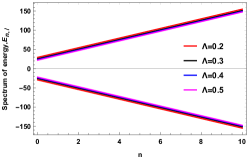
(a)

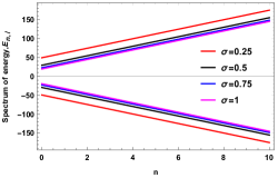
(b)

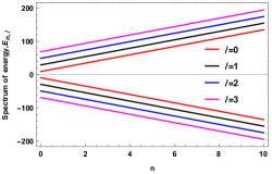
(c)

Figure 1: The energy spectrum $E_{n,\ell}^{\pm}$ for the relation given in equation (49), where the parameters are set as $k=M=1$ and $\rho_{0}=0.25$.

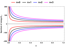
(d)

(e)

Figure 2: The energy spectrum $E_{n,\ell}^{\pm}$ for the relation given in equation (49), where the parameters are set as $k=M=1$ and $\rho_{0}=0.25$.

Equation (46) is the Bessel second-order differential equation whose solution is well-known. The solution is $\psi_{1}=c_{1}\,J_{\tau}(\Lambda\,\rho)+c_{2}\,Y_{\tau}(\lambda\,\rho)$ [71, 72], where $J_{\tau}$ and $Y_{\tau}$ are the Bessel functions of the first and second kind, respectively. It is also well-known that the Bessel function of the second kind is undefined at the origin $\rho=0$ but first kind is finite. Therefore, the requirement of the wave function $\psi_{1}(\rho)$ at the origin implies that the constant $c_{2}\to 0$. Therefore, the regular solution of the above differential equation is given by

$$\psi_{1}(\rho)=c_{1}\,J_{\tau}(\lambda\,\rho)\,.$$ (47)

We aim to confine the motion of scalar particles within a region characterized by a hard-wall confining potential. This confinement is particularly significant, as it provides an excellent approximation when investigating the quantum properties of systems, such as gas molecules and other particles inherently constrained within a defined spatial domain. The hard-wall confinement is defined by a condition specifying that at a certain axial distance, $\rho=\rho_{0}$, the radial wave function $\Psi$ becomes zero, i. e., $\Psi(\rho=\rho_{0})=0$. The study of the hard-wall potential has proven valuable in various contexts, including its examination on scalar fields under non-inertial effects [50], studies of the Klein-Gordon oscillator under cosmic string effects [49], examinations of the Dirac neutral particle [74, 75, 76], studies on the harmonic oscillator in an elastic medium [77], analogous to the Landau–Aharonov–Casher system in cosmic string space-time [78], and investigations into the behavior of Dirac and Klein-Gordon oscillators [79]. This exploration of the hard-wall potential in diverse scenarios enriches our understanding of its impact on quantum systems, providing insights into the behavior of scalar particles subject to this form of confinement. To obtain the energy levels of bound states from the boundary condition, let us take a fixed $\rho=\rho_{0}$ sufficiently large in such a way that we can consider $\lambda\,\rho_{0}>>1$.

Hence, by accepting this approximation $\lambda\,\rho_{0}>>1$, we can write the Bessel function of the first kind in the form [71, 72]

$$J_{\iota}(\lambda\,\rho_{0})\propto\cos\Big{(}\lambda\,\rho_{0}-\frac{\tau\,\pi}{2}-\frac{\pi}{4}\Big{)}.$$ (48)

Therefore, substituting this asymptotic form (48) into the equation (47) and using the boundary condition $\psi_{1}(\rho=\rho_{0})=0$, we obtain after simplification

$$E_{n,\ell}=\pm\,\sqrt{M^{2}+k^{2}+\Big{(}2\,n+\frac{3}{2}+\frac{|\ell|}{\sqrt{2\,\Lambda}\,|\sigma|}\Big{)}^{2}\,\frac{\pi^{2}}{4\,\rho^{2}_{0}}\Bigg{]}},$$ (49)

where $n=0,1,2,3,....$.

We have plotted Figure 1 to illustrate the energy eigenvalue (49) of DKP fields, by changing values of he cosmological constant $\Lambda$ (Fig: 1(a)), the topology parameter $\sigma$ (Fig: 1(b)), and the orbital quantum number $\ell$. We have observed a linear increase in the nature of the energy level, with increasing levels shifting downward (Fig: 1(a)-1(b)) and upward (Fig: 1(c)). In Figure 2, we have presented the energy spectrum with respect to the cosmological constant (Fig: 2(a)) and the topology parameter (Fig: 2(b)) for different quantum number $n$.

3 DKP-Lambda Oscillator

In this section, we study spin-0 relativistic DKP-oscillator fields in BML space-time backgrond. This oscillator is studied by nonminimal substitution $-i\,\vec{\nabla}_{\alpha}\to\Big{(}-i\,\vec{\nabla}_{\alpha}-i\,M\,\omega\,\eta^{0}\,\vec{\rho}\Big{)}$ or the radial momentum operator $\partial_{\rho}\to(\partial_{\rho}+M\,\omega\,\eta^{0}\,\rho)$, where $\omega$ is the oscillator frequency and $\eta^{0}$ is related with $\beta^{0}$. It is worth mentioning that this DKP-oscillator has been investigated by numerous authors in curved space-time, such as Gödel and Gödel-type solutions, topological defects background produced by cosmic strings and global monopoles (see, Refs. [80, 31, 32, 23, 81]), and in non-commutative phase space [82]. In terms of four-vector, this substitution will be

$$\partial_{\mu}\rightarrow\partial_{\mu}+M\omega X_{\mu}\eta^{0},$$ (50)

where the four-vector is defined by

$$X_{\mu}=\left(0,\rho,0,0\right).$$ (51)

And

$$\eta^{0}=2\left(\beta^{0}\right)^{2}-{\bf I}.$$ (52)

Therefore, the DKP-oscillator equation is described by

$$\left[i\,\widetilde{\beta}^{\mu}\left(\partial_{\mu}+M\,\omega\,X_{\mu}\,\eta^{0}+\frac{1}{2}\,\omega_{\mu ab}\,\left[\beta^{a},\beta^{b}\right]\,\right)-M\right]\psi=0.$$ (53)

Explicitly writing this equation (53) as follows:

$$\left[i\,\widetilde{\beta}^{0}\,\partial_{t}+i\,\widetilde{\beta}^{1}\,\left(\partial_{\rho}+M\,\omega\,\rho\,\eta^{0}\right)+i\,\widetilde{\beta}^{2}\left(\partial_{\varphi}+\frac{1}{2}\,\omega_{\varphi\,ab}\,\left[\beta^{a},\beta^{b}\right]\right)+i\,\widetilde{\beta}^{3}\,\partial_{z}-M\right]\psi=0.$$ (54)

That can be written as

$$\Bigg{[}i\,\beta^{0}\,\partial_{t}+i\,\beta^{1}\,(\partial_{\rho}+M\,\omega\,\eta^{0}\,\rho)+i\frac{\beta^{2}}{\sigma\,\sin\left(\sqrt{2\Lambda}\rho\right)}\left\{\partial_{\varphi}-\sigma\,\left(\sqrt{2\Lambda}\right)\,\cos\left(\sqrt{2\Lambda}\rho\right)\left(\beta^{1}\beta^{2}-\beta^{2}\beta^{1}\right)\right\}$$

$$+i\beta^{3}\partial_{z}-M\Bigg{]}\psi=0,$$ (55)

Substituting the wave function (36) and flat $\beta^{a}$ matrices, we obtain the following set of equations:

$$E\,\psi_{2}-i\,\left[\partial_{\rho}+M\,\omega\,\rho+\frac{\left(\sqrt{2\Lambda}\right)}{\tan\left(\sqrt{2\Lambda}\rho\right)}\right]\,\psi_{3}+\left[\frac{\ell}{\sigma\,\sin\left(\sqrt{2\Lambda}\rho\right)}\right]\,\psi_{4}+k\,\psi_{5}=M\,\psi_{1}.$$ (56)

$$E\,\psi_{1}=M\,\psi_{2}.$$ (57)

$$i\,\left(\partial_{\rho}-M\,\omega\,\rho\right)\,\psi_{1}=M\,\psi_{3}.$$ (58)

$$-\frac{|\ell|}{|\sigma|\,\sin\left(\sqrt{2\Lambda}\rho\right)}\,\psi_{1}=M\,\psi_{4}.$$ (59)

$$-k\,\psi_{1}=M\,\psi_{5}.$$ (60)

Decoupled the above set of equations, we obtain the following differential equation:

$$\left[\left(\partial_{\rho}+M\,\omega\,\rho+\frac{\left(\sqrt{2\Lambda}\right)}{\tan\left(\sqrt{2\Lambda}\rho\right)}\right)\left(\partial_{\rho}-M\,\omega\,\rho\right)-\frac{\ell^{2}}{\sigma^{2}\,\sin^{2}\left(\sqrt{2\Lambda}\rho\right)}+\lambda^{2}\right]\psi_{1}=0.$$ (61)

That can be writeen as

$$\left[\frac{\partial^{2}}{\partial\rho^{2}}+\frac{\left(\sqrt{2\Lambda}\right)}{\tan\left(\sqrt{2\Lambda}\rho\right)}\frac{\partial}{\partial\rho}-\left(M\,\omega\,\rho\right)^{2}-\frac{\ell^{2}}{\sigma^{2}\,\sin^{2}\left(\sqrt{2\Lambda}\rho\right)}-\frac{M\,\omega\,\rho\,\left(\sqrt{2\Lambda}\right)}{\tan\left(\sqrt{2\Lambda}\rho\right)}+\lambda^{2}-M\,\omega\right]\psi_{1}=0$$ (62)

where $\lambda=\sqrt{E^{2}-M^{2}-k^{2}}$.

To solve the above second-order differential equation, we employ approximation into the trigonometric functions up to the first order. However, one can try to find general solution of this differential equation by doing a substitution $u=\cos\left(\sqrt{2\Lambda}\rho\right)$ which we omitted here. Therefore, the above differential equation after approximation becomes

$$\left[\frac{\partial^{2}}{\partial\rho^{2}}+\frac{1}{\rho}\,\frac{\partial}{\partial\rho}-M^{2}\,\omega^{2}\,\rho^{2}-\frac{\tau^{2}}{\rho^{2}}+\xi\right]\psi_{1}=0,$$ (63)

where

$$\tau=\frac{|\ell|/|\sigma|}{\sqrt{2\Lambda}},\quad\xi=\lambda^{2}-2\,M\,\omega.$$ (64)

Transforming to a new variable via $s=M\,\omega\,\rho^{2}$ into the above equation (63) results the following differential equation form:

$$\psi^{\prime\prime}_{1}(s)+\frac{(d_{1}-\,d_{2}\,s)}{s\,(1-d_{3}\,s)}\,\psi^{\prime}_{1}(s)+\frac{\Big{(}-\zeta_{1}\,s^{2}+\zeta_{2}\,s-\zeta_{3}\Big{)}}{s^{2}\,(1-d_{3}\,s)^{2}}\,\psi_{1}(s)=0,$$ (65)

where $d_{1}=1$, $d_{2}=0=d_{3}$ and

$$\zeta_{1}=\frac{1}{4},\quad\zeta_{2}=\frac{\xi}{4\,M\,\omega},\quad\zeta_{3}=\frac{\tau^{2}}{4}.$$ (66)

Equation (65) is homogeneous second-order differential equation which can be solves using the Nikiforov-Uvarov method [73]. Following this method, we obtain the following expression of the energy spectrum given by

$$E_{n,\ell}=\pm\,\sqrt{M^{2}+k^{2}+4\,M\,\omega\,\Bigg{(}n+1+\frac{|\ell|}{2\,\sqrt{2\Lambda}\,|\sigma|}\Bigg{)}}.$$ (67)

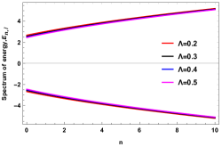
(a)

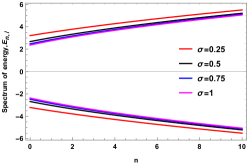
(b)

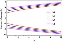
(c)

Figure 3: The energy spectrum $E_{n,\ell}^{\pm}$ for the relation given in equation (67), where the parameters are set as $k=M=1$ .

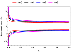
(d)

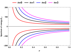
(e)

Figure 4: The energy spectrum $E_{n,\ell}^{\pm}$ for the relation given in equation (67), where the parameters are set as $k=M=1$.

The corresponding radial wave function will be

$$\psi_{1\,n,\ell}(\rho)=\mathcal{N}\,\left(M\,\omega\,\rho^{2}\right)^{\frac{|\ell|}{2\,\sqrt{2\Lambda}\,|\sigma|}}\,Exp\left[-\frac{1}{2}\,M\,\omega\,\rho^{2}\right]\,L^{\Big{(}\frac{|\ell|}{2\,\sqrt{2\Lambda}\,|\sigma|}\Big{)}}_{n}(M\,\omega\,\rho^{2}),$$ (68)

where $\mathcal{N}$ is the normalization constant.

Therefore, other components of the wave functions are given by

$$\psi_{2\,n,\ell}(\rho)=\frac{E_{n,\ell}}{M}\,\psi_{1\,n,\ell}.$$ (69)

$$\psi_{3\,n,\ell}(\rho)=\frac{i}{M}\,\psi^{\prime}_{1\,n,\ell}-i\,\omega\,\rho\,\psi_{1\,n,\ell}.$$ (70)

$$\psi_{4\,n,\ell}(\rho)=-\frac{|\ell|}{|\sigma|\,\sin\left(\sqrt{2\Lambda}\,\rho\right)}\,\psi_{1\,n,\ell}.$$ (71)

$$\psi_{5\,n,\ell}(\rho)=-\frac{k}{M}\,\psi_{1\,n,\ell}.$$ (72)

We have generated Figure 3 to illustrate the energy eigenvalue (67) of DKP oscillator fields, varying the values of the cosmological constant $\Lambda$ (Fig: 3(a)), the topology parameter $\sigma$ (Fig: 3(b)), and the orbital quantum number $\ell$. Our observations indicated a linear increase in the energy level, with increasing levels shifting downward (Fig: 3(a)-3(b)) and upward (Fig: 3(c)). In Figure 4, we presented the energy spectrum with respect to the cosmological constant (Fig: 4(a)) and the topology parameter (Fig: 4(b)) for different quantum numbers $n$.

4 Conclusions

The study of both relativistic and non-relativistic limits of quantum systems in curved space has been a focal point in theoretical physics since long time. The gravitational field generated by curved space exerts significant influences on the quantum behaviors of spin-0 Bosonic fields, fermionic fields, and spin-1 fields. In addition, if the investigation is carried out in the presence of topological defects, then the eigenvalue solution of the quantum systems get modifications by these and break the degeneracy of the energy spectrum. Moreover, numerous authors introduced external uniform and non-uniform magnetic fields and presented the modified eigenvalue solution of these particles. In addition, many authors considered interaction potential of various kinds (both electromagnetic and non-electromagnetic potential) and showed that the energy eigenvalues of Bosonic and Fermionic fields get shifted. The eigenvalue solutions of the quantum system, obtained by solving the wave equations, undergo modifications due to the effects of the gravitational field, topological defects, interacting potential and external magnetic field and deviating the results from those obtained in flat space background. In this analysis, we focused on a four-dimensional magnetic space-time featuring a cosmological constant. There are only a handful Einstein-Maxwell solutions without and with cosmological constants have been known in the general relativity. The considered space-time is an example of electrovacuum Einstein-Maxwell solution in general relativity whose magnetic field strength is associated with two parameters $(\sigma,\Lambda)$ of the geometry.

In section 2, we discussed the motion of spin-0 quantum particles described by the DKP equation and solved it in the background of magnetic space-time. We showed that the derived equation is the Bessel second-order differential equation whose solution is well-known. By imposing hard-wall confining potential condition, we determined the energy eigenvalue of spin-0 DKP fields given in equation (49). In section 3, we discussed the DKP-oscillator in the same magnetic space-time background. This oscillator field is studied by a nonminimal substitution in the momentum operator. We derived the radial equation and solved it through the parametric Nikiforov-Uvarov method. We have seen that the energy eigenvalue of DKP oscillator fields given in equation (67) is influenced by the parameters $(\sigma,\Lambda)$ and the oscillator frequency $\omega$. We represented these energy profiles by illustrating a few graphs and have shown the nature of these by choosing different values of parameters $(\sigma,\Lambda)$ and the quantum number $n$.

In this context, intriguing results have been presented regarding the relativistic quantum system within the framework of a magnetic universe. The system under analysis exhibits the characteristics of a spin-0 Bosonic field and a Bosonic oscillator field, both influenced by a positive cosmological constant ($\Lambda>0$), indicative of a de-Sitter (dS) space background. The current phase of the universe’s expansion is marked by acceleration, a phenomenon validated by the $\Lambda$CDM model. The interrelation between these theories remains an enigma in theoretical physics, presenting a compelling avenue for further exploration and understanding.

Data Availability Statement

No new data were analysed.

Conflict of Interest

No conflict of interests in this paper.

Funding Statement

No fund has received for this work.

References

- [1] A. Einstein, Annalen Phys. 49, 769 (1916)https://doi.org/10.1002/20andp.200590044.
- [2] B. P. Abbott et al, Phys Rev Lett 116, 061102 (2016)https://doi.org/10.1103/PhysRevLett.116.061102.
- [3] K. Akiyama et al, Astrophys J Lett 875, L1 (2019)https://doi.org/10.3847/2041-8213/ab0f43.
- [4] R. P. Feynman, and A. R. Hibbs, Quantum mechanics and path integrals, Dover Publications Inc. (1965).
- [5] K. Gödel, Rev. Mod. Phys. 21, 447 (1949)https://doi.org/10.1103/RevModPhys.21.447.
- [6] N. Drukker, B. Fiol and J. Simon, JCAP 10,12 (2004)https://doi.org/10.1088/1475-7516/2004/10/012.
- [7] M. M. Som and A. K. Raychaudhuri, Proc. R. Soc. A 304, 81 (1968)https://doi.org/10.1098/rspa.1968.0073.
- [8] C. C. Barros Jr., Eur. Phys. J. C 42, 119 (2005)https://doi.org/10.1140/epjc/s2005-02252-7.
- [9] F. Ahmed, Commun. Theor. Phys. 68, 735 (2017)https://doi.org/10.1088/0253-6102/68/6/735.
- [10] L. C. N. Santos, C. E. Mota and C. C. Barros, Adv. High Energy Phys. 2019, 2729352 (2019) https://doi.org/10.1155/2019/2729352.
- [11] G. de A. Marques and V. B. Bezerra, Phys. Rev. D 66, 105011 (2002)https://doi.org/10.1103/PhysRevD.66.105011.
- [12] A. Boumali and N. Messai, Can. J. Phys. 92, 1460 (2014)https://doi.org/10.1134/S0202289321030026.
- [13] E. R. Figueiredo Medeiros and E. R. B. de Mello, Eur. Phys. J. C 72, 2051 (2012)https://doi.org/10.1140/epjc/s10052-012-2051-9.
- [14] C. O. Edet et al., Results in Physics 39, 105749 (2022)https://doi.org/10.1016/j.rinp.2022.105749.
- [15] F. Ahmed, Mol. Phys. 120, Article: e2124935 (2022)https://doi.org/10.1080/00268976.2022.2124935.
- [16] F. Ahmed, Phys. Scr. 98, 015403 (2023)https://doi.org/10.1088/1402-4896/aca6b3.
- [17] R. J. Duffin, Phys. Rev. 54, 1114 (1938)https://doi.org/10.1103/PhysRev.54.1114.
- [18] N. Kemmer, Proc. R. Soc. London, Ser. A 173, 91 (1939)https://doi.org/10.1098/rspa.1939.0131.
- [19] G. Petiau, Acad. R. Belg. Cl. Sci. Mém. Collect. 8, 16 (1939).
- [20] R. F. Guertin, Phys. Rev. D 15, 1518 (1977)https://doi.org/10.1103/PhysRevD.15.1518.
- [21] Y. Nedjadi and R. C. Barrett, J. Phys. G 19, 87 (1993)https://doi.org/10.1088/0954-3899/19/1/006.
- [22] W. Greiner, Relativistic Quantum Mechanics: Wave Equations, Springer, Berlin (2000).
- [23] M. Hosseinpour and H. Hassanabadi. Adv. High Energy Phys. 2018, 2959354 (2018)https://doi.org/10.1140/epjc/s10052-018-5574-x.
- [24] A. Boumali, A. Bouzenada, S. Zare, and H. Hassanabadi, Phys. A: Stat. Mech., 628, 129134 (2023)https://doi.org/10.1016/j.physa.2023.129134.
- [25] S. Zare, H. Hassanabadi, and M. de Montigny. Gen. Relativ. Gravit., 52, 1-20 (2020)https://doi.org/10.1007/s10714-020-02676-0.
- [26] S. Zare, H. Hassanabadi, and M. de Montigny, Int. J. Mod. Phys. A 35, 2050195 (2020)https://doi.org/10.1142/S0217751X2050195X.
- [27] F. Ahmed, and H. Hassanabadi, Mod. Phys. Lett. A 35,2050031 (2020)https://doi.org/10.1142/S0217732320500315.
- [28] H. Sobhani, H. Hassanabadi, and W. S. Chung, Few-Body Syst.61,1-12 (2020)https://doi.org/10.1007/s00601-019-1537-5.
- [29] M. de Montigny, M. Hosseinpour, and H. Hassanabadi, Int. J Mod. Phys. A 31, 1650191 (2016)https://doi.org/10.1142/S0217751X16501918.
- [30] L. B. Castro, Eur Phys J C 75, 287 (2015)https://doi.org/10.1140/epjc/s10052-015-3507-5.
- [31] L. B. Castro, Eur Phys J C 76, 61 (2016) https://doi.org/10.1140/epjc/s10052-016-3904-4.
- [32] H. Hassanabadi, M. Hosseinpour, and M. de Montigny, Eur Phys J Plus 132, 541 (2017) https://doi.org/10.1140/epjp/i2017-11831-y.
- [33] A. Boumali and H. Aounallah, Adv. High Energy Phys. 2018, 1031713 (2018) https://doi.org/10.1155/2018/1031763.
- [34] C. Thompson and R. C. Duncan, Mon. Notices R Astron. Soc. 275, 255 (1995) https://doi.org/10.1093/mnras/275.2.255.
- [35] C. Kouveliotou et al., Nature, 393, 235 (1998) https://doi.org/10.1038/30410.
- [36] U. Gürsoy, D. Kharzeev and K. Rajagopal, Phys. Rev. C, 89, 054905 (2014) https://doi.org/10.1103/PhysRevC.89.054905.
- [37] A. Bzdak and V. Skokov, Phys. Lett. B 710, 171 (2012) https://doi.org/10.1016/j.physletb.2012.02.065.
- [38] V. Voronyuk, V. D. Toneev, W. Cassing, E. L. Bratkovskaya, V. P. Konchakovski and S. A. Voloshin, Phys. Rev. C, 83, 054911 (2011).
- [39] T. Gutsunaev and V. Manko, Phys. Lett. A 123, 215 (1987) https://doi.org/10.1016/0375-9601(87)90063-6.
- [40] T. Gutsunaev and V. Manko, Phys. Lett. A 132, 85 (1988) https://doi.org/10.1016/0375-9601(88)90257-5.
- [41] W. B. Bonnor, Proc. Phys. Soc. A 67, 225 (1954) https://doi.org/10.1088/0370-1298/67/3/305.
- [42] M. Melvin, Phys. Lett. 8, 65 (1964) https://doi.org/10.1016/0031-9163(64)90801-7.
- [43] M. Žofka, Phys. Rev. D 99, 044058 (2019) https://doi.org/10.1103/PhysRevD.99.044058.
- [44] L. Parker, Phys. Rev. Lett. 44, 1559 (1980) https://doi.org/10.1103/PhysRevLett.44.1559.
- [45] N. D. Birrell, N. D. Birrell and P. Davies, Quantum fields in curved space, Cambridge University Press, Cambridge (1982).
- [46] E. Elizalde, Phys. Rev. D 36, 1269 (1987) https://doi.org/10.1103/physrevd.36.1269.
- [47] S. Chandrasekhar, Proc. R. Soc. Lond. A 349, 571 (1976) https://doi.org/10.1098/rspa.1976.0090.
- [48] L. C. N. Santos and C. C. Barros Jr., Eur. Phys. J. C 77, 186 (2017) https://doi.org/10.1140/epjc/s10052-017-4732-x.
- [49] L. C. N. Santos and C. C. Barros Jr., Eur. Phys. J. C 78, 13 (2018) https://doi.org/10.1140/epjc/s10052-017-5476-3.
- [50] R. L. L. Vitória and K. Bakke, Eur. Phys. J. C 78, 175 (2018) https://doi.org/10.1140/epjc/s10052-018-5658-7.
- [51] F. Ahmed, Int. J. Mod. Phys. A 37, 2250186 (2022) https://doi.org/10.1142/S0217751X2250186X.
- [52] F. Ahmed, Commun. Theor. Phys.75, 025202 (2023) https://doi.org/10.1088/1572-9494/aca650.
- [53] Y. Yang, Z.-W. Long, Q.-K. Ran, H. Chen, Z.-L. Zhao, and C.-Y. Long, Int. J. Mod. Phys. A 36, 2150023 (2021) https://doi.org/10.1142/S0217751X21500238.
- [54] A. R. Soares, R. L. L. Vitória, and H. Aounallah, Eur. Phys. J. Plus 136, 966 (2021) https://doi.org/10.1140/epjp/s13360-021-01965-0.
- [55] A. Bouzenada, A. Boumali, Ann. Phys. (NY) 452, 169302 (2023) https://doi.org/10.1016/j.aop.2023.169302.
- [56] A. Bouzenada, A. Boumali, R. L. L. Vitoria, F. Ahmed and M. Al-Raeei, Nucl. Phys. B 994, 116288 (2023) https://doi.org/10.1016/j.nuclphysb.2023.116288.
- [57] A. Bouzenada, A. Boumali and F. Serdouk, Theor. Math. Phys,216, 1055 (2023) https://doi.org/10.1134/S0040577923070115.
- [58] A. Bouzenada, A. Boumali, and E. O. Silva, Ann. Phys. (N. Y.) 458,169479 (2023) https://doi.org/10.1016/j.aop.2023.169479.
- [59] V. B. Bezerra, M. S. Cunha, L. F. F. Freitas, C. R. Muniz and M. O. Tahim, Mod. Phys. Lett. A 32, 1750005 (2016) https://doi.org/10.1142/S0217732317500055.
- [60] L. C. N. Santos and C. C. Barros Jr., Int. J. Mod. Phys. A 33, 1850122 (2018) https://doi.org/10.1142/S0217751X18501221.
- [61] E. O. Pinho and C. C. Barros Jr., Eur. Phys. J. C. 83, 745 (2023) https://doi.org/10.1140/epjc/s10052-023-11907-y.
- [62] P. Sedaghatnia, H. Hassanabadi, and F. Ahmed, Eur. Phys. J. C. 79, 541 (2019) https://doi.org/10.1140/epjc/s10052-019-7051-6.
- [63] A. Guvendi, S. Zare, and H. Hassanabadi, Phys. Dark Univ. 38, 101133 (2022) https://doi.org/10.1016/j.dark.2022.101133.
- [64] R. L. L. Vitória and K. Bakke, Eur. Phys. J. Plus 133, 490 (2018) https://doi.org/10.1140/epjp/i2018-12310-9.
- [65] L. C. N. Santos and C. C. Barros Jr., Eur. Phys. J. C 76, 560 (2016) https://doi.org/10.1140/epjc/s10052-016-4409-x.
- [66] M. Astorino, JHEP 06 (2012) 086 https://doi.org/10.1007/JHEP06(2012)086.
- [67] F. Ahmed and A. Bouzenada, arXiv:2312.06612 [gr-qc] https://doi.org/10.48550/arXiv.2312.06612.
- [68] F. Ahmed and A. Bouzenada, arXiv:2312.06615 [gr-qc] https://doi.org/10.48550/arXiv.2312.06615.
- [69] L. G. Barbosa, and C. C. Barros Jr., arXiv:2311.11148 [gr-qc] https://doi.org/10.48550/arXiv.2311.11148.
- [70] L. G. Barbosa, and C. C. Barros Jr., arXiv:2310.04883 [gr-qc] https://doi.org/10.48550/arXiv.2310.04883..
- [71] M. Abramowitz and I. A. Stegun, Handbook of Mathematical Functions with Formulas, Graphs, and Mathematical Tables, New York: Dover (1972).
- [72] G. B. Arfken, H. J. Weber and F. E. Harris, Mathematical Methods for Physicists, Elsevier (2012).
- [73] A. F. Nikiforov and V. B. Uvarov, Special Functions of Mathematical Physics, Birkhauser (1988) https://doi.org/10.1007/978-1-4757-1595-8.
- [74] K. Bakke, Open Physics 11, 1589 (2013) https://doi.org/10.2478/s11534-013-0313-2.
- [75] K. Bakke, Mod. Phys. Lett. B 27, 1350018 (2013) https://doi.org/10.1142/S0217984913500188.
- [76] K. Bakke, Ann. Phys. (NY) 346, 51 (2014) https://doi.org/10.1016/j.aop.2014.04.003.
- [77] A. V. D. M. Maia and K. Bakke, Phys. B 531, 213 (2018) https://doi.org/10.1016/j.physb.2017.12.045.
- [78] K. Bakke, Int. J. Theor. Phys. 54, 2119 (2015) https://doi.org/10.1007/s10773-014-2418-9.
- [79] E. A. F. Bragança, R. L. L. Vitória, H. Belich and E. R. Bezerra de Mello, Eur. Phys. J. C 80, 206 (2020) https://doi.org/10.1140/epjc/s10052-020-7774-4.
- [80] M. Hosseinpour, H. Hassanabadi, and F. M. Andrade, Eur Phys J C 78, 93 (2018) https://doi.org/10.1140/epjc/s10052-018-5574-x.
- [81] A. Boumali, J. Math. Phys. 49, 022302 (2008) https://doi.org/10.1063/1.2841324, Erratum: ibid 54, 099902 (2013) https://doi.org/10.1063/1.4821200.
- [82] G. R. de Melo, M. de Montigny, and E. S. Santos, J. Phys.: Conf. Ser. 343, 012028 (2012) https://doi.org/10.1088/1742-6596/343/1/012028.