Street Gaussians for Modeling Dynamic Urban Scenes

Abstract

This paper aims to tackle the problem of modeling dynamic urban street scenes from monocular videos. Recent methods extend NeRF by incorporating tracked vehicle poses to animate vehicles, enabling photo-realistic view synthesis of dynamic urban street scenes. However, significant limitations are their slow training and rendering speed, coupled with the critical need for high precision in tracked vehicle poses. We introduce Street Gaussians, a new explicit scene representation that tackles all these limitations. Specifically, the dynamic urban street is represented as a set of point clouds equipped with semantic logits and 3D Gaussians, each associated with either a foreground vehicle or the background. To model the dynamics of foreground object vehicles, each object point cloud is optimized with optimizable tracked poses, along with a dynamic spherical harmonics model for the dynamic appearance. The explicit representation allows easy composition of object vehicles and background, which in turn allows for scene editing operations and rendering at 133 FPS (1066$\times$1600 resolution) within half an hour of training. The proposed method is evaluated on multiple challenging benchmarks, including KITTI and Waymo Open datasets. Experiments show that the proposed method consistently outperforms state-of-the-art methods across all datasets. Furthermore, the proposed representation delivers performance on par with that achieved using precise ground-truth poses, despite relying only on poses from an off-the-shelf tracker. The code is available at https://zju3dv.github.io/street_gaussians/.

1 Introduction

Modeling dynamic 3D streets from images has many important applications, such as city simulation, autonomous driving, and gaming. For instance, the digital twin of city streets can be used as the simulation environment for self-driving vehicles, thereby reducing the training and test costs. These applications require us to efficiently reconstruct 3D street models from captured data and render high-quality novel views in real-time.

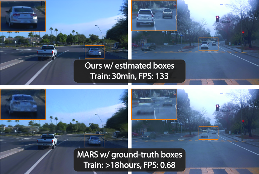
Figure 1: Rendering results on the Waymo dataset [44]. With only estimated trajectories, our method produces high-quality rendering at 133 FPS (1066$\times$1600) within half an hour of training. Current SOTA method [55] requires accurate ground-truth trajectories, and has low training and rendering speed.

With the development of neural scene representations, there have been some methods [27, 45, 37, 34, 69] that attempt to reconstruct street scenes with neural radiance fields [30]. To improve the modeling capability, Block-NeRF [45] divides the target street into several blocks and represents each one with a NeRF network. Although this strategy enables photo-realistic rendering of large-scale street scenes, Block-NeRF suffers from long training time due to the large amount of network parameters. Moreover, it cannot handle dynamic vehicles on the street, which are crucial aspects in autonomous driving environment simulation.

Recently, some methods [33, 62, 55, 19] propose to represent dynamic street scenes as compositional neural representations that consist of foreground moving cars and static background. To handle the dynamic car, they leverage tracked vehicle poses to establish the mapping between the observation space and the canonical space, where they use NeRF networks to model the car’s geometry and appearance. As a result, these methods are sensitive to the accuracy of tracked bounding boxes. In addition, they are still limited to the high training cost and low rendering speed.

In this work, we propose a novel explicit scene representation for reconstructing dynamic 3D street scenes from images. The basic idea is utilizing point clouds to build dynamic scenes, which significantly increases the training and rendering efficiency while decreasing the dependency on the accuracy of tracked vehicle poses. Specifically, we decompose urban street scenes into the static background and moving vehicles, which are separately built based on 3D Gaussians [16]. To handle the dynamics of foreground vehicles, we model their geometry as a set of points with optimizable tracked vehicle poses, where each point stores learnable 3D Gaussian parameters. Furthermore, the time-varying appearance is represented by a 4D spherical harmonics model that uses a time series function to predict spherical harmonics coefficients at any time step. Thanks to the dynamic Gaussian representation, we can faithfully reconstruct the target urban street within half an hour and achieve real-time rendering (133FPS@1066x1600).

Building upon the proposed scene representation, we further develop a tracked pose optimization strategy. The optimizable input tracked poses ensure a better alignment between the rendered and input videos. Experiments reveal that our method yields comparable results to that achieved with ground-truth poses, while only utilizing poses from an off-the-shelf tracker [53], thanks to the better gradient propagation facilitated by our explicit representation.

We evaluate the proposed method on Waymo Open [44] (Waymo) and KITTI [13] datasets, which present dynamic street scenes with complex vehicle motions and various environment conditions. Across all datasets, our approach achieves state-of-the-art performance in terms of rendering quality, while being rendered over 100 times faster than previous methods [55, 33]. Furthermore, detailed ablations and scene editing applications are conducted to demonstrate the effectiveness of proposed components and the flexibility of the proposed representation, respectively.

Overall, this work makes the following contributions:

• We propose Street Gaussians, a novel scene representation for modeling complex dynamic street scenes, which efficiently reconstructs and renders high-fidelity urban street scenes in real-time.

• We develop a tracked pose optimization strategy along with a 4D spherical harmonics appearance model to handle the dynamics of moving vehicles.

• We conduct comprehensive comparisons and ablations on several challenging datasets, demonstrating our approach’s new state-of-the-art performance and the effectiveness of the proposed components.

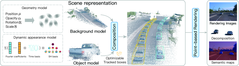
Figure 2: Overview of Street Gaussians. The dynamic urban street scene is represented as a set of point-based background and foreground objects with optimizable tracked vehicle poses. Each point is assigned with a 3D Gaussian [16] including position, opacity, and covariance consisting of rotation and scale to represent the geometry. To represent the appearance, we assign each background point with a spherical harmonics model while the foreground points are associated with a dynamic spherical harmonics model. The explicit point-based representation allows easy composition of separate models, which enables real-time rendering of high-quality images and semantic maps (optional if 2D semantic information is provided during training), as well as the decomposition of foreground objects for editing applications.

2 Related work

Simulation environments for autonomous driving.  Existing self-driving simulation engines such as CARLA [9] or AirSim [40] suffer from costly manual effort to create virtual environments and the lack of realism in the generated data. In recent years, a lot of effort has been put into building sensor simulations from autonomous driving data captured in real scenes. Some works [29, 61, 10] concentrate on LiDAR simulation by aggregating LiDAR and reconstructing textured primitives. However, they have difficulty handling high-resolution images and usually produce noisy appearance. Other works [64, 7, 49] reconstruct objects from multi-view images and LiDAR input, which can be interacted with other environments. However, these methods are restricted to existing images and fail to render novel views. Some methods utilize neural fields to perform multiply tasks including view synthesis [62, 33, 15], perception [19, 12, 69], generation [41, 32, 57, 60, 21] and inverse rendering [50] on driving scenes. However, they struggle with long training time and slow rendering speed. In contrast, Our method focuses on performing real-time rendering of dynamic urban street scenes, which is crucial for autonomous driving simulation.

Static scene modeling.  Neural scene representation proposes to represent 3D scenes with neural networks, which can model complex scenes from images through differentiable rendering. NeRF [30, 3, 4, 5, 31] represents continuous volumetric scenes with MLP networks and achieves impressive rendering results. Some works have been proposed to extend NeRF to urban scenes [37, 45, 14, 27, 26, 34, 47]. DNMP [27] models the scene with deformable mesh primitives initialized by voxelizing point clouds. NeuRas [26] takes scaffold mesh as input and optimizes the neural texture field to perform fast rasterization. Point-based rendering works [38, 18, 1, 8, 23] define learned neural descriptors on point clouds and perform differentiable rasterization with a neural renderer. However, they require dense point clouds as input and generate blurry results under regions with low point counts. A very recent work 3D Gaussian Splatting (3D GS) [16] defines a set of anisotropic Gaussians in 3D world and performs adaptive density control to achieve high-quality rendering results with only sparse point clouds input. However, 3D GS assumes the scene to be static and can not model dynamic moving objects.

Dynamic scene modeling.  Recent methods build 4D neural scene representation on single-object scenes [42, 35, 11, 22, 2, 24, 36, 25]. Some works learn a scene decomposition of outdoor scenes under the supervision of optical flow [48] or vision transformer feature [59]. However, their scene decomposition can not be edited, limiting the applications for autonomous driving simulation. Another line of works model the scene as the composition of moving object models and a background model [33, 19, 55, 62, 56] with neural fields, which is most similar to us. However, they require accurate object trajectories and suffer from high memory cost and slow inference speed. Point-based dynamic scene rendering is also investigated recently [58, 67]. Concurrent to our work [63, 65, 52, 28] also extend 3D GS to dynamic scenes, but they build their models on small-scale data while we focus on large-scale urban street scenes.

3 Method

Given a sequence of images captured from a moving vehicle in an urban street scene, our goal is to develop a model capable of generating photorealistic images for any given input time step and any viewpoints. Towards this objective, we propose a novel scene representation, named Street Gaussians, specifically designed for representing dynamic street scenes. As shown in the Figure 2, we represent a dynamic urban street scene as a set of point clouds, each corresponding to either the static background or a moving vehicle (Section 3.1). The explicit point-based representation allows easy composition of separate models, enabling real-time rendering as well as the decomposition of foreground objects for editing applications (Section 3.2). The proposed scene representation can be effectively trained using only RGB images, along with tracked vehicle poses from an off-the-shelf tracker, enhanced by our tracked vehicle pose optimization strategy (Section 3.3).

3.1 Street Gaussians

In this section, we seek to find a dynamic scene representation that can be quickly constructed and rendered in real-time. Previous methods [55, 19] typically face challenges with low training and rendering speed as well as accurate tracked vehicle poses. To tackle this problem, we propose a novel explicit scene representation, named Street Gaussians, which is built upon 3D Gaussians [16]. In Street Gaussians, we represent the static background and each moving vehicle object with a separate neural point cloud.

In the following, we will first focus on the background model, elaborating on several common attributes that are shared with the object model. Subsequently, we will delve into the dynamic aspects of the object model’s design.

Background model.

The background model is represented as a set of points in the world coordinate system. Each point is assigned with a 3D Gaussian to softly represent the continuous scene geometry and color. The Gaussian parameters consist of a covariance matrix $\bm{\Sigma}_{b}$ and a position vector $\bm{\mu}_{b}\in\mathbb{R}^{3}$, which denotes the mean value. To avoid invalid covariance matrix during optimization, each covariance matrix is further reduced to a scaling matrix $\mathbf{S}_{b}$ and a rotation matrix $\mathbf{R}_{b}$, where $\mathbf{S}_{b}$ is characterized by its diagonal elements. and $\mathbf{R}_{b}$ is converted into a unit quaternion. The covariance matrix $\bm{\Sigma}_{b}$ can be recovered from $\mathbf{S}_{b}$ and $\mathbf{R}_{b}$ as:

$$\bm{\Sigma}_{b}=\mathbf{R}_{b}\mathbf{S}_{b}{\mathbf{S}_{b}}^{T}{\mathbf{R}_{b}}^{T}.$$ (1)

Apart from the position and covariance matrix, each Gaussian is also assigned with an opacity value $\alpha_{b}\in\mathbb{R}$ and a set of spherical harmonics coefficients $\mathbf{z}_{b}=(z_{m,l})^{m:-\ell\leq m\leq\ell}_{l:0\leq\ell\leq\ell_{max}}$ to represent scene geometry and appearance. To obtain the view-dependent color, the spherical harmonics coefficients are further multiplied by the spherical harmonics basis functions projected from the view direction. To represent 3D semantic information, each point is added with a semantic logit $\bm{\beta}_{b}\in\mathbb{R}^{M}$, where $M$ is the number of semantic classes.

Object model.

Consider a scene containing $N$ moving foreground object vehicles. Each object is represented with a set of optimizable tracked vehicle poses and a point cloud, where each point is assigned a 3D Gaussian, semantic logits, and a dynamic appearance model.

The Gaussian properties of both the object and the background are similar, sharing the same meaning for opacity $\alpha_{o}$ and scale matrix $\mathbf{S}_{o}$. However, their position, rotation, and appearance models differ from those of the background model. The position $\bm{\mu}_{o}$ and rotation $\mathbf{R}_{o}$ are defined in the object local coordinate system. To transform them into the world coordinate system (the background’s coordinate system), we introduce the definition of tracked poses for objects. Specifically, the tracked poses of vehicles are defined as a set of rotation matrices $\{\mathbf{R}_{t}\}_{t=1}^{N_{t}}$ and translation vectors $\{\mathbf{T}_{t}\}_{t=1}^{N_{t}}$, where $N_{t}$ represents the number of frames. The transformation can be defined as:

$$\bm{\mu}_{w} =\mathbf{R}_{t}\bm{\mu}_{o}+\mathbf{T}_{t},$$ (2)

$$\mathbf{R}_{w} =\mathbf{R}_{o}\mathbf{R}_{t}^{T},$$

where $\bm{\mu}_{w}$ and $\mathbf{R}_{w}$ are the position and rotation of the corresponding object Gaussian in the world coordinate system, respectively. After transformation, the object’s covariance matrix $\bm{\Sigma}_{w}$ can be obtained by Eq. 1 with $\mathbf{R}_{w}$ and $\mathbf{S}_{o}$. Note that we also found the tracked vehicle poses from the off-the-shelf tracker to be noisy. To address this issue, we treat the tracked vehicle poses as learnable parameters. We detail it in Section 3.3.

Simply representing object appearance with the spherical harmonics coefficients is insufficient for modeling the appearance of moving vehicles, as shown in Figure 3, because the appearance of a moving vehicle is influenced by its position in the global scene. One straightforward solution is to use separate spherical harmonics to represent the object for each timestep. However, this representation will significantly increase the storage cost. Instead, we introduce the 4D spherical harmonics model by replacing each SH coefficient $z_{m,l}$ with a set of fourier transform coefficients $\bm{f}\in\mathbb{R}^{k}$ where $k$ is the number of fourier coefficient. Given timestep $t$, $z_{m,l}$ is recovered by performing real-valued Inverse Discrete Fourier Transform:

$$z_{m,l}=\sum_{i=0}^{k-1}\bm{f}_{i}\cos\left(\frac{i\pi}{N_{t}}t\right).$$ (3)

With the proposed model, we encode time information into appearance without high storage cost.

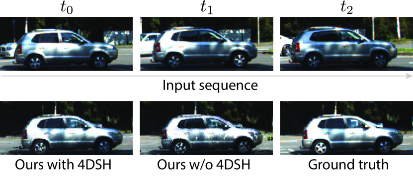
Figure 3: Effect of 4D SH (spherical harmonics) model. The first row presents the input sequence, showcasing varying appearances. The second row demonstrates the impact of utilizing the proposed 4D SH model on the rendering results. Significant artifacts can be observed if the 4D SH model is absent.

The semantic representation of the object model is different from that of the background model. The main difference is that the semantic of the object model is a one-dimensional scalar $\beta_{o}$ instead of a $M$-dimensional vector $\bm{\beta}_{b}$ like the background model. This semantic model for the foreground object vehicle model can be considered as a binary classification or a confidence prediction problem because there are only two semantic categories for the object, i.e., vehicle semantic class (from the tracker) and non-vehicle.

3.2 Rendering of Street Gaussians

To render Street Gaussians, we need to aggregate the contribution of each model to render the final image. Previous methods [33, 19, 62, 55] require compositional rendering with complex raymarching because of neural field representation. Instead, Street Gaussians can be rendered by contacting all the point clouds and projecting them to 2D image space. Specifically, given a rendered time step $t$, we first compute spherical harmonics Eq. 3 , and transform the object point cloud into the world coordinate system using and Eq. 2 according to tracked vehicle pose $(\mathbf{R}_{t},\mathbf{T}_{t})$. Then we concatenate the background point cloud and the transformed object point clouds to form a new point cloud. To project this point cloud to 2D image space with camera extrinsic $\mathbf{W}$ and intrinsic $\mathbf{K}$, we compute the 2D Gaussian for each point in the point cloud:

$$\bm{\mu}^{\prime} =\mathbf{K}\mathbf{W}\bm{\mu},$$ (4)

$$\bm{\Sigma}^{\prime} =\mathbf{J}\mathbf{W}\bm{\Sigma}\mathbf{W}^{T}\mathbf{J}^{T},$$

where $\mathbf{J}$ is the Jacobian matrix of $\mathbf{K}$. $\mu^{\prime}$ and $\Sigma^{\prime}$ are the position and covariance matrix in 2D image space, respectively. Point-based $\alpha$-blending for each pixel is used to compute the color $\mathbf{c}$:

$$\mathbf{c}=\sum_{i\in N}\mathbf{c}_{i}\alpha_{i}\prod_{j=1}^{i-1}(1-\alpha_{j}),$$ (5)

Here $\alpha_{i}$ is the opacity $\alpha$ multiplied by the probability of the 2D Gaussian [66] and $\mathbf{c}_{i}$ is the color computed from spherical harmonics $\mathbf{z}$ with the view direction.

The semantic map can be rendered simply by changing color $c$ in Eq 5 to semantic logits $\bm{\beta}$.

3.3 Training

Tracking pose optimization.

Positions and covariance matrices of the object Gaussians during rendering in Section 3.2 are closely correlated with the tracked pose parameters as shown in Eq 2. However, bounding boxes produced by the tracker model are generally noisy. Directly using them to optimize our scene representation leads to degradation in rendering quality. As a result, we treat tracked poses as learnable parameters by adding a learnable transformation to each transformation matrix. Specifically, $\mathbf{R}_{t}$ and $\mathbf{T}_{t}$ in Eq 2 are replaced by $\mathbf{R}_{t}^{{}^{\prime}}$ and $\mathbf{T}_{t}^{{}^{\prime}}$ which are defined as:

$$\mathbf{R}_{t}^{\prime} =\mathbf{R}_{t}\Delta\mathbf{R}_{t},$$ (6)

$$\mathbf{T}_{t}^{\prime} =\mathbf{T}_{t}+\Delta\mathbf{T}_{t},$$

where $\Delta\mathbf{R}_{t}$ and $\Delta\mathbf{T}_{t}$ are the learnable transformation. We represent $\Delta\mathbf{T}_{t}$ as a 3D vector and $\Delta\mathbf{R}_{i}$ as a rotation matrix converted from yaw offset angle $\Delta\theta_{t}$. Gradients of these transformations can be directly obtained without any implicit function or intermediate processes, which do not require any extra computation during back-propagation.

Loss function.

We jointly optimize our scene representation and tracked poses using the following loss function:

$$\mathcal{L}=\mathcal{L}_{\text{color}}+\lambda_{1}\mathcal{L}_{\text{sem}}+\lambda_{2}\mathcal{L}_{\text{reg}}.$$ (7)

In Eq 7, $\mathcal{L}_{\text{color}}$ is the reconstruction loss between rendered and observed images. $\mathcal{L}_{\text{sem}}$ is an optional per-pixel softmax-cross-entropy loss between rendered semantic logits and input 2D semantic segmentation predictions [20]. In order to prevent noisy input semantic labels from influencing the geometry, we stop the gradients of $\mathcal{L}_{\text{sem}}$ back to $\alpha$ in Eq 5. $\mathcal{L}_{\text{reg}}$ is an entropy regularization term used to remove floaters and enhance decomposition effects. Please refer to the supplementary material for the details. In practice, we set $\lambda_{1}=0.1$ and $\lambda_{2}=0.1$.

4 Implementation details

Initialization.  We use LiDAR point cloud captured by ego vehicle as initialization. Specifically, we first collect points inside the bounding boxes and transform them into the local coordinate system to initialize each object model. Then we downsample the remaining aggregated point cloud with a voxel size of 0.15m and filter out invisible points for the background model. The colors of LiDAR point cloud are obtained by projecting to the corresponding image plane and querying the pixel value. Due to the limited coverage of LiDAR point clouds over large areas, we also incorporate SfM [39] point cloud to handle distant regions.

Densification and pruning.  We follow [16] to apply adaptive control during optimization. Original 3D Gaussians set the scene radius based on camera poses, which is not suitable for large-scale urban scenes. As a result, we obtain the radius of the background model by the LiDAR point cloud while the radius of the object model is determined by the bounding box scale. In order to prevent object Gaussians from growing to occluded areas, for each object model we sample a set of points as a probability distribution function. During optimization, Gaussians with sampled points outside the bounding box will be pruned.

5 Experiments

5.1 Experimental Setup

We train Street Gaussians for 30000 iterations with Adam optimizers [17] following the learning rate configurations of 3D Gaussians [16]. The learning rate of translation transformation $\Delta\mathbf{T}_{t}$ and rotation transformation $\Delta\mathbf{R}_{t}$ are set to 0.005 and 0.001, which decay exponentially to $5e^{-5}$ and $1e^{-5}$ respectively. All the experiments are conducted on one RTX 4090 GPU.

Datasets.  We conduct experiments on Waymo Open Dataset [44] and KITTI benchmarks [13]. On the Waymo Open Dataset, we select 6 recording sequences with large amounts of moving objects, significant ego-car motion and complex lighting conditions. All sequences have a length of around 100 frames. We select every 10th image in the sequence as the test frames and use the remaining for training. As we find that our baseline methods [33, 55] suffer from high memory cost when training with high-resolution images, we downscale the input images to $1066\times 1600$. On KITTI [13] and Vitural KITTI 2 [6], we follow the settings of MARS [55] and evaluate our methods with different train/test split settings. We use the bounding boxes generated by the detector[54] and tracker [53] on Waymo dataset and use the officially provided object tracks from KITTI.

Baseline methods.  We compare our methods with three recent methods. (1) NSG [33] represents background as multi-plane images and use per-object learned latent codes with a shared decoder to model moving objects. (2) MARS [55] builds the scene graph based on Nerfstudio [46]. (3) 3D Gaussians [16] models the scene with a set of anisotropy gaussians. Both NSG and MARS are trained and evaluated using ground truth bounding boxes, we try different versions of their implementations and report the best result for each sequence. We also replace the SfM point cloud in 3D Gaussians with the same input as our method for fair comparison. See supplementary material for details.

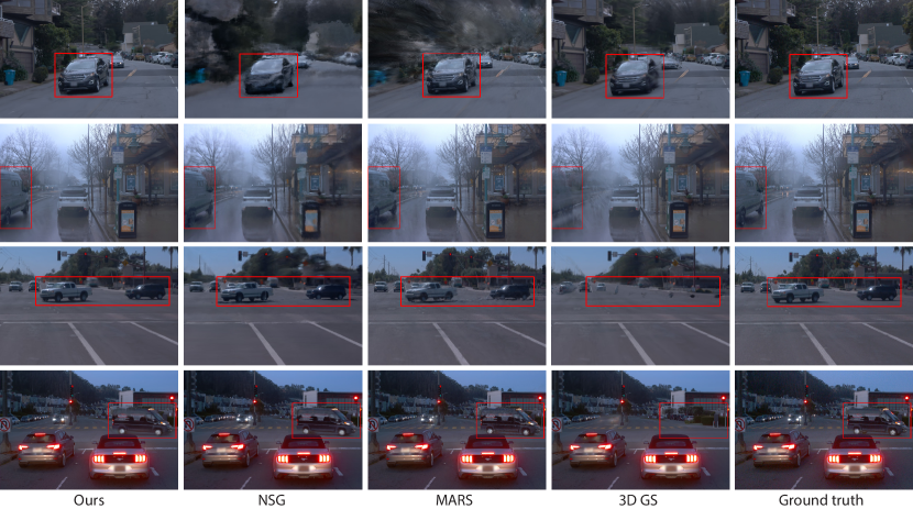
Figure 4: Qualitative comparisons on the Waymo [44] dataset. NSG [33] and MARS [55] often produce blurry and distorted results. 3D GS [16] fails to handle dynamic objects and generates ghosting artifacts in these cases. In contrast, our approach significantly outperforms other methods with high fidelity and sharp details.

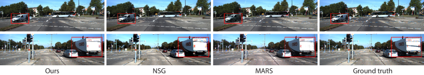
Figure 5: Qualitative comparisons on the KITTI [13] dataset.

	3D GS [16]	NSG [33]	MARS [55]	Ours
PSNR$\uparrow$	29.95	30.23	31.37	34.54
PSNR*$\uparrow$	17.74	22.05	23.07	25.16
SSIM$\uparrow$	0.907	0.866	0.904	0.936
LPIPS$\downarrow$	0.140	0.331	0.246	0.091
FPS$\uparrow$	227	0.47	0.68	133

Table 1: Quantitative results on the Waymo [44] dataset. The rendering image resolution is $1066\times 1600$. “PSNR*” denotes the PSNR of moving objects.

5.2 Comparisons with the State-of-the-art

Tables 1, 2 present the comparison results of our method with baseline methods [16, 33, 55] in terms of rendering quality and rendering speed. We adopt PSNR, SSIM and LPIPS [68] as metrics to evaluate rendering quality. To better evaluate the quality of moving objects, we project 3D bounding boxes to 2D image plane and calculate the loss only on pixels inside the projected box, which is denoted as PSNR* in our experiments. For all the metrics, our model achieves the best performance among all the methods. Moreover, our method renders two magnitudes faster than MARS and NSG. Although 3D GS is faster than our method, it can only support static scenes and the result of moving objects degrades significantly.

Figures 4, 5 show the qualitative results of our method and baselines. NSG and MARS suffer from blurry and distorted results, which is especially marked when the camera has a large motion. This should be attributed to their model lacking sufficient expressive capability when the scene is complex. 3D GS fails to handle dynamic objects and generates ghosting artifacts in these cases. In contrast, our method can generate high-quality novel views with high fidelity and details.

		KITTI - 75%				KITTI - 50%				KITTI - 25%
		PSNR$\uparrow$	SSIM$\uparrow$	LPIPS$\downarrow$		PSNR$\uparrow$	SSIM$\uparrow$	LPIPS$\downarrow$		PSNR$\uparrow$	SSIM$\uparrow$	LPIPS$\downarrow$
3D GS [16]		19.19	0.737	0.172		19.23	0.739	0.174		19.06	0.730	0.180
NSG* [33]		21.53	0.673	0.254		21.26	0.659	0.266		20.00	0.632	0.281
MARS* [55]		24.23	0.845	0.160		24.00	0.801	0.164		23.23	0.756	0.177
Ours		25.79	0.844	0.081		25.52	0.841	0.084		24.53	0.824	0.090
		VKITTI2 - 75%				VKITTI2 - 50%				VKITTI2 - 25%
		PSNR$\uparrow$	SSIM$\uparrow$	LPIPS$\downarrow$		PSNR$\uparrow$	SSIM$\uparrow$	LPIPS$\downarrow$		PSNR$\uparrow$	SSIM$\uparrow$	LPIPS$\downarrow$
3D GS [16]		21.12	0.877	0.097		21.11	0.874	0.097		20.84	0.863	0.098
NSG* [33]		23.41	0.689	0.317		23.23	0.679	0.325		21.29	0.666	0.317
MARS* [55]		29.79	0.917	0.088		29.63	0.916	0.087		27.01	0.887	0.104
Ours		30.10	0.935	0.025		29.91	0.932	0.026		28.52	0.917	0.034

Table 2: Quantitative results on KITTI [13] and VKITTI2 [6] datasets. We strictly follow the experimental setting of MARS [55] and borrow results of MARS [55] and NSG [33] from it. The rendering image resolution is 375 $\times$ 1242.

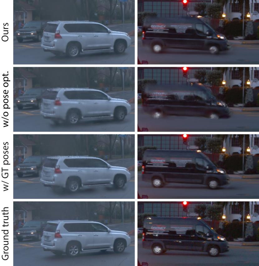
Figure 6: Visual ablation results on the Waymo [44] dataset. The results indicate that optimizing tracked poses improves the quality. “opt.” denotes optimization.

5.3 Ablations and Analysis

We validate our algorithm’s design choices on all six select sequences from the Waymo dataset. Tables 3 present the quantitative results. The influence of optimizing tracked poses.  Experimental results in Table 3 show that without optimizable tracked poses the rendering quality degrades much. This is because inaccurate poses make the object model supervised under the wrong pixel value. Figure 3 shows some visual results. To further validate the effectiveness of optimizing tracked poses, we compare our method with a variant that uses ground truth poses from the dataset. As shown in row2 Table 3, the performance gap between our complete model and the model trained with ground truth poses is small, which indicates the effectiveness of our pose optimization strategy. It is interesting to notice that the LPIPS metric of our complete model issue even better than the model trained with ground truth poses, a plausible explanation is that tracked poses of real-world data is obtained from manual annotations where noisy results still exist.

	PSNR$\uparrow$	PSNR*$\uparrow$	SSIM$\uparrow$	LPIPS$\downarrow$
Ours w/o pose opt.	34.05	23.37	0.934	0.094
Ours w/o 4DSH	34.38	24.72	0.935	0.093
Ours w/ GT pose	34.57	25.24	0.936	0.092
Complete model	34.54	25.16	0.936	0.091

Table 3: Ablation studies on the Waymo [44] dataset. Metrics are averaged over all the sequences on the Waymo dataset. “PSNR*” denotes the PSNR of moving objects. “opt.” denotes optimization. Please refer to Section 5.3 for details.

Visual results of the influence of tracked pose optimization is shown in Figure 6. The first two rows indicate that treating tracked poses as learnable parameters help the object model synthesize more texture details and reduce rendering artifacts. Models trained directly with tracked poses suffer from inaccurate positions in the world frame. Moreover, In comparison with images rendered with ground truth poses, our results with optimized tracked poses are comparable or even better on challenging regions like the rear of the white vehicle or the logo of the black vehicle in Figure 6.

Effectiveness of 4D spherical harmonics.  Results in Table 3 indicate that our 4D spherical harmonics appearance model can refine the rendering quality. This situation becomes particularly evident when the object interacts with environmental lighting as shown in Figure 3. Our model can generate smooth shadows on the car while the rendering results without 4D spherical harmonics are much noisier.

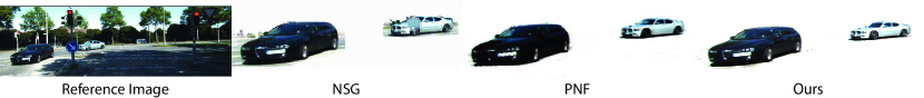
Figure 7: Decomposition results on the KITTI [13] dataset. NSG [33] cannot decompose clean foreground objects while PNF [19] produces blurry results. Instead, our method successfully decomposes the foreground objects and produces high fidelity rendering results.

5.4 Applications

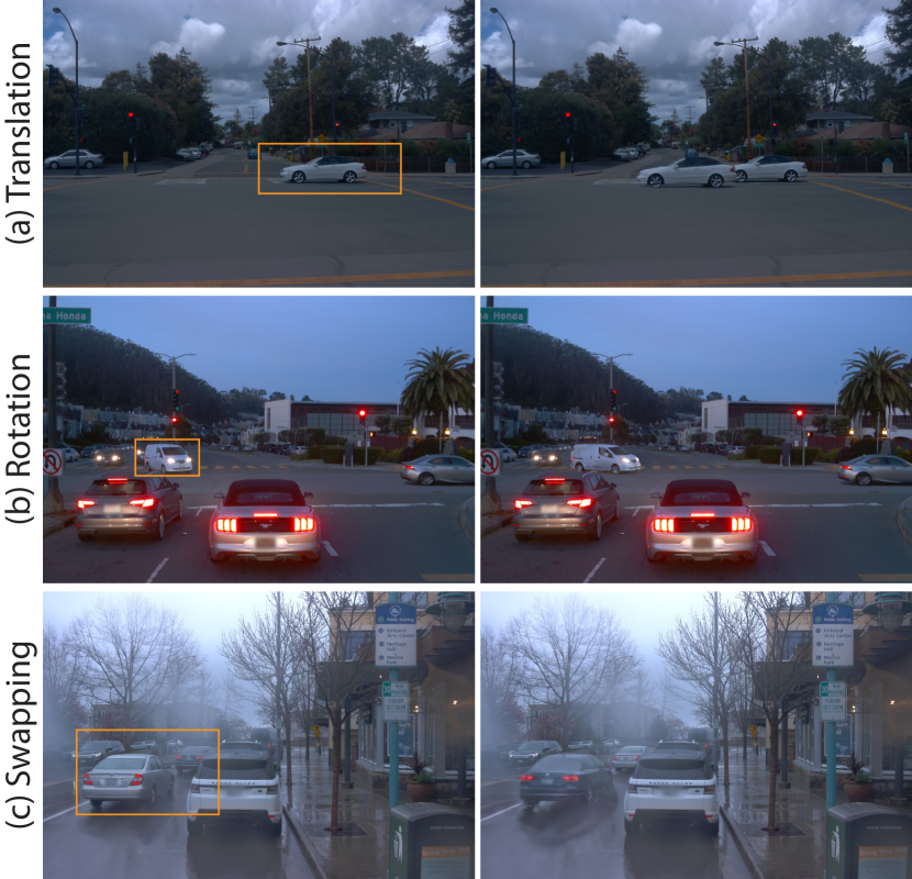
Figure 8: Editing operations on the Waymo [44] dataset. Images in the left and right columns represent the results before and after editing. Our method supports various editing operations, including translation, rotation and swapping.

Street Gaussians can be applied to multiple tasks in computer vision including object decomposition, semantic segmentation and scene editing. Object Decomposition.  We compare the decomposition results of our method with NSG [33] and PNF [19] under KITTI dataset. As shown in Figure 7, NSG fails to disentangle foreground objects from the background and the result of PNF is lack of details. In contrast, our method can produce high-fidelity decomposed rendering results.

Scene editing.  Our scene representation enables various types of scene editing operations. We can translate the vehicle (Figure 8 (a)), rotate the heading of the vehicle (Figure 8 (b)) and swap the vehicles with another one (Figure 8 (c)).

Semantic Segmentation.  We compare the quality of our rendered semantic map with the semantic prediction from Video-K-Net [20] on KITTI dataset. Our semantic segmentation model is trained with results from Video K-Net. Qualitative and quantitative results are shown in Figure 9 and Table 4. Our rendered semantic maps achieve better performance thanks to our 3D semantic representation.

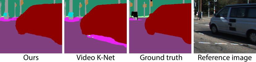
Figure 9: Visual semantic segmentation results on the KITTI [13] dataset. It can be observed that our method achieves better performance, particularly in ambiguous areas such as shadows due to our ability to fuse semantic information in 3D.

Method	VKN ground-truth	VKN rendered	Ours
mIoU $\uparrow$	57.94	53.81	58.81

Table 4: Quantitative segmentation results on the KITTI [13] dataset. “VKN ground-truth” and “VKN rendered” denote semantic prediction results of Video K-Net with ground-truth images and our rendered images, respectively.

6 Conclusion and Discussion

This paper introduced Street Gaussians, an explicit scene representation for modeling dynamic urban street scenes. The proposed representation separately models the background and foreground vehicles as a set of neural point clouds. This explicit representation allows easy compositing of object vehicles and background, enabling scene editing and real-time rendering within half an hour of training. Furthermore, we demonstrate that the proposed scene representation can achieve comparable performance to that achieved using precise ground-truth poses, using only poses from an off-the-shelf tracker. Detailed ablation and comparison experiments are conducted on several datasets, demonstrating the effectiveness of the proposed method.

This work also has some known limitations. First, our method is limited to reconstructing rigid dynamic scenes, such as static streets with only moving vehicles, and cannot handle non-rigid dynamic objects like walking pedestrians. Future work could consider employing more complex dynamic scene modeling methods [51], to address this issue. Second, the proposed method is dependent on the recall rate of off-the-shelf trackers. If some vehicles are missed, our pose optimization strategy cannot compensate for this. We leave this problem to future work.

Appendix

Appendix A More implementation details

Baselines.

On Waymo Open Dataset [44], we find that the results of NSG [33] and MARS [55] is better when using a separate neural field for each object compared with shared decoder and per-object optimized latent codes, especially when the number of moving objects is relatively high. One plausible reason is that the tracking results provided by the Waymo dataset do not differentiate between different types of vehicles, Therefore, the shared decoder needs to fit objects with significant differences in shape, which makes the optimization process more complex. As a result, We use the original NeRF [30] and Nerfacto [46] to represent each object model in NSG and MARS respectively. For MARS, we also add depth loss following their implementation.

Hyperparameters.

We set the number of fourier coefficients $k$ as 5 to maintain a balance between performance and storage cost. Due to the relatively less intense view-dependent effect on urban scene compared to dataset in 3D Gaussian [16], we reduce the SH degree to 1 to prevent overfitting. For the remaining parameters, we use the default values from the official implementation of 3D Gaussian [16].

Evaluation metrics.

Figure 10 visually illustrates the calculation method of the PSNR* metric in our experiments. For fair comparison, both our method and the baselines are evaluated using the mask obtained from ground-truth tracked boxes.

Regularization loss.

The regularization term in our loss function is defined as an entropy loss on the accumulated alpha values of decomposed foreground objects which can be generated in parallel during training. We add this loss after the adaptive control process to help Street Gaussians better distinguish foreground and background following [43]. Figure 11 shows the qualitative results, which demonstrates the effect of this regularization term.

Object semantic.

We learn a confidence score between 0 and 1 for each Gaussian in the object model. The logits of the vehicle semantic class output by each Gaussian is a constant $C$ multiplied by this confidence score. We set $C$ as 100 in our experiments. To merge the one-dimensional scalar $\beta_{o}$ with the M-dimensional vector $\beta_{b}$ of background, we convert $\beta_{o}$ to a M-dimensional one-hot vector for the vehicle label during rendering.

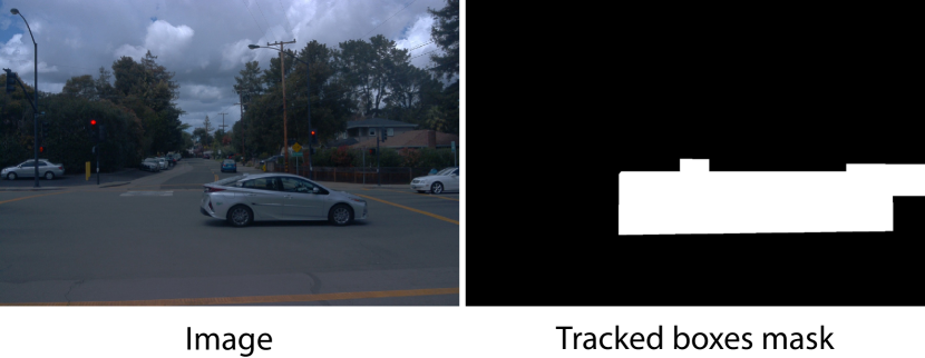
Figure 10: Illustration of PSNR*. We project the 3D tracked boxes to 2D image plane and obtain the mask above. We calculate the MSE (Mean Squared Error) for the pixels within the mask to get the value of PSNR*.

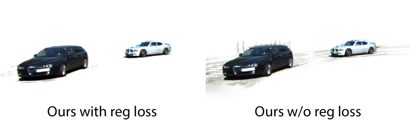
Figure 11: Effect of regularization loss on decomposition results. “reg loss” denotes regularization loss. Adding this term can significantly remove ghosty artifacts around the vehicle.

Appendix B Additional experiments

Influence of initial point cloud.

We train one sequence from Waymo dataset using LiDAR point cloud or SfM point cloud as initialization respectively. The SfM point cloud of background is built by running Colmap [39] on input training images. We randomly sample points inside the bounding box for moving objects as we find that the recovered point cloud from Colmap is very sparse.

Figure 12 and Table 5 show the qualitative and quantitative results. Our method can generate high-fidelity images using either methods. SfM point cloud can achieve better results on background as it can better capture the geometry of the scene while LiDAR point cloud can model moving objects better as it is denser. Our approach combines them to leverage their respective strengths.

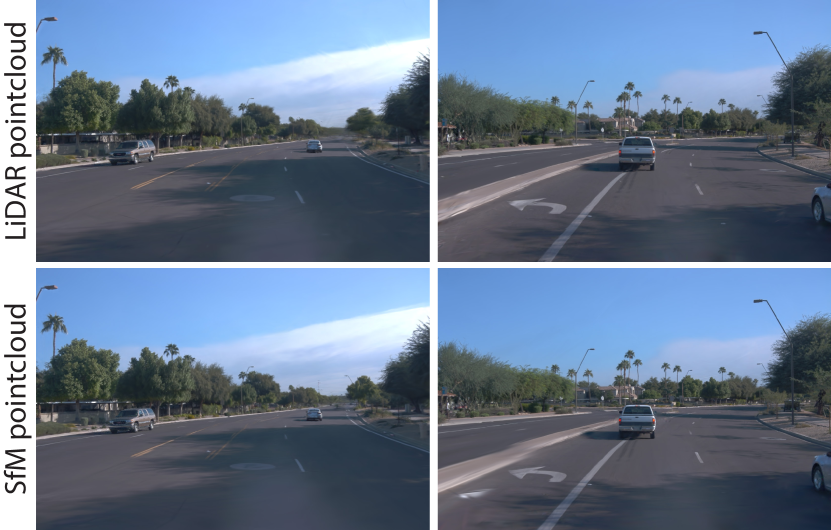
Figure 12: Qualitative results of different initial point clouds.

	PSNR$\uparrow$	PSNR*$\uparrow$	SSIM$\uparrow$	LPIPS$\downarrow$
LiDAR point cloud	31.09	23.31	0.914	0.097
SfM point cloud	31.43	22.80	0.917	0.097

Table 5: Quantitative results of different initial point clouds

Extrapolation results.

In Figure 13, we show some qualitative results of novel view synthesis when the camera is far away from input image sequence on Waymo dataset. Please see our supplementary video for more details.

	Sequence A
	w/o pose opt.	with pose opt.	with GT poses
MARS [55]	21.01	22.91	24.97
Ours	23.91	26.12	25.34
	Sequence B
	w/o pose opt.	with pose opt.	with GT poses
MARS [55]	19.61	21.06	22.17
Ours	20.29	22.14	22.59

Table 6: More ablation studies on tracking pose optimization. We report the results of PSNR* on two scenes from Waymo dataset. “opt.” denotes optimization.

Analysis of optimizing tracked poses.

As discussed in our main paper, we observe that our explicit representation facilitates the optimization of tracked vehicle poses with ease. Herein, we extend our study to explore the impact of an implicit representation on optimizing tracked vehicle poses. The experimental results, as presented in Table 6, indicate that while the inclusion of our pose optimization strategy with implicit representation improves outcomes, there remains a noticeable gap compared to experiments using ground truth tracked poses. However, the proposed method, employing tracked poses from an off-the-shelf tracker, achieves results comparable to those using GT poses. This success can be attributed to the more efficient propagation of gradients through explicit representations in relation to tracked poses.

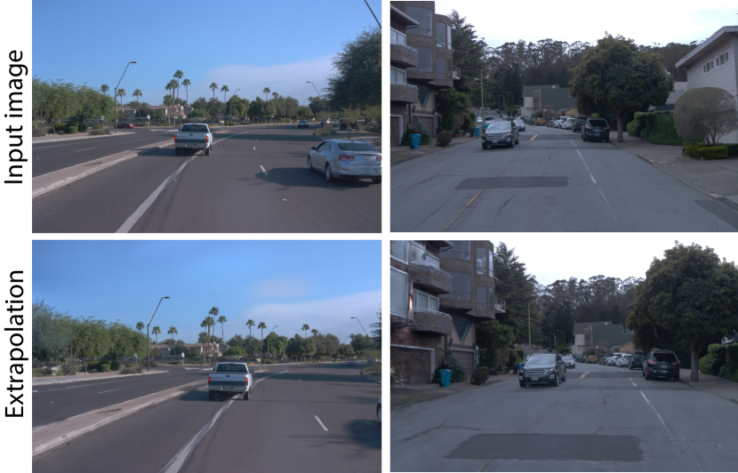
Figure 13: Qualitative results of novel view synthesis with significant differences from the training set. We translate the camera for 2 meters and rotate it for 30 degrees.

References

- Aliev et al. [2020] Kara-Ali Aliev, Artem Sevastopolsky, Maria Kolos, Dmitry Ulyanov, and Victor Lempitsky. Neural point-based graphics. In ECCV, 2020.
- Attal et al. [2023] Benjamin Attal, Jia-Bin Huang, Christian Richardt, Michael Zollhoefer, Johannes Kopf, Matthew O’Toole, and Changil Kim. HyperReel: High-fidelity 6-DoF video with ray-conditioned sampling. In CVPR, 2023.
- Barron et al. [2021] Jonathan T. Barron, Ben Mildenhall, Matthew Tancik, Peter Hedman, Ricardo Martin-Brualla, and Pratul P. Srinivasan. Mip-nerf: A multiscale representation for anti-aliasing neural radiance fields. ICCV, 2021.
- Barron et al. [2022] Jonathan T. Barron, Ben Mildenhall, Dor Verbin, Pratul P. Srinivasan, and Peter Hedman. Mip-nerf 360: Unbounded anti-aliased neural radiance fields. CVPR, 2022.
- Barron et al. [2023] Jonathan T. Barron, Ben Mildenhall, Dor Verbin, Pratul P. Srinivasan, and Peter Hedman. Zip-nerf: Anti-aliased grid-based neural radiance fields. ICCV, 2023.
- Cabon et al. [2020] Yohann Cabon, Naila Murray, and Martin Humenberger. Virtual kitti 2. arXiv preprint arXiv:2001.10773, 2020.
- Chen et al. [2021] Yun Chen, Frieda Rong, Shivam Duggal, Shenlong Wang, Xinchen Yan, Sivabalan Manivasagam, Shangjie Xue, Ersin Yumer, and Raquel Urtasun. Geosim: Realistic video simulation via geometry-aware composition for self-driving. In CVPR, 2021.
- Dai et al. [2020] Peng Dai, Yinda Zhang, Zhuwen Li, Shuaicheng Liu, and Bing Zeng. Neural point cloud rendering via multi-plane projection. In CVPR, 2020.
- Dosovitskiy et al. [2017] Alexey Dosovitskiy, German Ros, Felipe Codevilla, Antonio Lopez, and Vladlen Koltun. Carla: An open urban driving simulator. In Conference on robot learning, pages 1–16. PMLR, 2017.
- Fang et al. [2020] Jin Fang, Dingfu Zhou, Feilong Yan, Tongtong Zhao, Feihu Zhang, Yu Ma, Liang Wang, and Ruigang Yang. Augmented lidar simulator for autonomous driving. IEEE Robotics and Automation Letters, 5(2):1931–1938, 2020.
- Fridovich-Keil et al. [2023] Sara Fridovich-Keil, Giacomo Meanti, Frederik Rahbæk Warburg, Benjamin Recht, and Angjoo Kanazawa. K-planes: Explicit radiance fields in space, time, and appearance. In CVPR, 2023.
- Fu et al. [2022] Xiao Fu, Shangzhan Zhang, Tianrun Chen, Yichong Lu, Lanyun Zhu, Xiaowei Zhou, Andreas Geiger, and Yiyi Liao. Panoptic nerf: 3d-to-2d label transfer for panoptic urban scene segmentation. In 3DV, pages 1–11. IEEE, 2022.
- Geiger et al. [2012] Andreas Geiger, Philip Lenz, and Raquel Urtasun. Are we ready for autonomous driving? the kitti vision benchmark suite. In CVPR, 2012.
- Guo et al. [2023] Jianfei Guo, Nianchen Deng, Xinyang Li, Yeqi Bai, Botian Shi, Chiyu Wang, Chenjing Ding, Dongliang Wang, and Yikang Li. Streetsurf: Extending multi-view implicit surface reconstruction to street views. arXiv preprint arXiv:2306.04988, 2023.
- Huang et al. [2023] Shengyu Huang, Zan Gojcic, Zian Wang, Francis Williams, Yoni Kasten, Sanja Fidler, Konrad Schindler, and Or Litany. Neural lidar fields for novel view synthesis. arXiv preprint arXiv:2305.01643, 2023.
- Kerbl et al. [2023] Bernhard Kerbl, Georgios Kopanas, Thomas Leimkühler, and George Drettakis. 3d gaussian splatting for real-time radiance field rendering. TOG, 42(4), 2023.
- Kingma and Ba [2014] Diederik P Kingma and Jimmy Ba. Adam: A method for stochastic optimization. arXiv preprint arXiv:1412.6980, 2014.
- Kopanas et al. [2021] Georgios Kopanas, Julien Philip, Thomas Leimkühler, and George Drettakis. Point-based neural rendering with per-view optimization. In CGF, pages 29–43. Wiley Online Library, 2021.
- Kundu et al. [2022] Abhijit Kundu, Kyle Genova, Xiaoqi Yin, Alireza Fathi, Caroline Pantofaru, Leonidas Guibas, Andrea Tagliasacchi, Frank Dellaert, and Thomas Funkhouser. Panoptic Neural Fields: A Semantic Object-Aware Neural Scene Representation. In CVPR, 2022.
- Li et al. [2022a] Xiangtai Li, Wenwei Zhang, Jiangmiao Pang, Kai Chen, Guangliang Cheng, Yunhai Tong, and Chen Change Loy. Video k-net: A simple, strong, and unified baseline for video segmentation. In CVPR, 2022a.
- Li et al. [2022b] Yuan Li, Zhi-Hao Lin, David Forsyth, Jia-Bin Huang, and Shenlong Wang. Climatenerf: Physically-based neural rendering for extreme climate synthesis. arXiv preprint arXiv:2211.13226, pages arXiv–2211, 2022b.
- Li et al. [2021] Zhengqi Li, Simon Niklaus, Noah Snavely, and Oliver Wang. Neural scene flow fields for space-time view synthesis of dynamic scenes. In CVPR, 2021.
- Li et al. [2023] Zhuopeng Li, Lu Li, and Jianke* Zhu. Read: Large-scale neural scene rendering for autonomous driving. In AAAI, 2023.
- Lin et al. [2022] Haotong Lin, Sida Peng, Zhen Xu, Yunzhi Yan, Qing Shuai, Hujun Bao, and Xiaowei Zhou. Efficient neural radiance fields for interactive free-viewpoint video. In SIGGRAPH Asia Conference Proceedings, 2022.
- Lin et al. [2023] Haotong Lin, Sida Peng, Zhen Xu, Tao Xie, Xingyi He, Hujun Bao, and Xiaowei Zhou. High-fidelity and real-time novel view synthesis for dynamic scenes. In SIGGRAPH Asia 2023 Conference Proceedings, pages 1–9, 2023.
- Liu et al. [2023] Jeffrey Yunfan Liu, Yun Chen, Ze Yang, Jingkang Wang, Sivabalan Manivasagam, and Raquel Urtasun. Neural scene rasterization for large scene rendering in real time. In ICCV, 2023.
- Lu et al. [2023] Fan Lu, Yan Xu, Guang Chen, Hongsheng Li, Kwan-Yee Lin, and Changjun Jiang. Urban radiance field representation with deformable neural mesh primitives. ICCV, 2023.
- Luiten et al. [2024] Jonathon Luiten, Georgios Kopanas, Bastian Leibe, and Deva Ramanan. Dynamic 3d gaussians: Tracking by persistent dynamic view synthesis. In 3DV, 2024.
- Manivasagam et al. [2020] Sivabalan Manivasagam, Shenlong Wang, Kelvin Wong, Wenyuan Zeng, Mikita Sazanovich, Shuhan Tan, Bin Yang, Wei-Chiu Ma, and Raquel Urtasun. Lidarsim: Realistic lidar simulation by leveraging the real world. In CVPR, 2020.
- Mildenhall et al. [2020] Ben Mildenhall, Pratul P. Srinivasan, Matthew Tancik, Jonathan T. Barron, Ravi Ramamoorthi, and Ren Ng. Nerf: Representing scenes as neural radiance fields for view synthesis. In ECCV, 2020.
- Müller et al. [2022] Thomas Müller, Alex Evans, Christoph Schied, and Alexander Keller. Instant neural graphics primitives with a multiresolution hash encoding. SIGGRAPH, 2022.
- Niemeyer and Geiger [2021] Michael Niemeyer and Andreas Geiger. Giraffe: Representing scenes as compositional generative neural feature fields. In CVPR, 2021.
- Ost et al. [2021] Julian Ost, Fahim Mannan, Nils Thuerey, Julian Knodt, and Felix Heide. Neural scene graphs for dynamic scenes. In CVPR, 2021.
- Ost et al. [2022] Julian Ost, Issam Laradji, Alejandro Newell, Yuval Bahat, and Felix Heide. Neural point light fields. CVPR, 2022.
- Park et al. [2021] Keunhong Park, Utkarsh Sinha, Peter Hedman, Jonathan T Barron, Sofien Bouaziz, Dan B Goldman, Ricardo Martin-Brualla, and Steven M Seitz. Hypernerf: A higher-dimensional representation for topologically varying neural radiance fields. arXiv preprint arXiv:2106.13228, 2021.
- Peng et al. [2023] Sida Peng, Yunzhi Yan, Qing Shuai, Hujun Bao, and Xiaowei Zhou. Representing volumetric videos as dynamic mlp maps. In CVPR, pages 4252–4262, 2023.
- Rematas et al. [2022] Konstantinos Rematas, Andrew Liu, Pratul P Srinivasan, Jonathan T Barron, Andrea Tagliasacchi, Thomas Funkhouser, and Vittorio Ferrari. Urban radiance fields. In CVPR, 2022.
- Rückert et al. [2022] Darius Rückert, Linus Franke, and Marc Stamminger. Adop: Approximate differentiable one-pixel point rendering. TOG, 41(4):1–14, 2022.
- Schonberger and Frahm [2016] Johannes L Schonberger and Jan-Michael Frahm. Structure-from-motion revisited. In CVPR, 2016.
- Shah et al. [2018] Shital Shah, Debadeepta Dey, Chris Lovett, and Ashish Kapoor. Airsim: High-fidelity visual and physical simulation for autonomous vehicles. In Field and Service Robotics: Results of the 11th International Conference, pages 621–635. Springer, 2018.
- Shen et al. [2023] Bokui Shen, Xinchen Yan, Charles R Qi, Mahyar Najibi, Boyang Deng, Leonidas Guibas, Yin Zhou, and Dragomir Anguelov. Gina-3d: Learning to generate implicit neural assets in the wild. In CVPR, 2023.
- Song et al. [2023] Liangchen Song, Anpei Chen, Zhong Li, Zhang Chen, Lele Chen, Junsong Yuan, Yi Xu, and Andreas Geiger. Nerfplayer: A streamable dynamic scene representation with decomposed neural radiance fields. TVCG, 29(5):2732–2742, 2023.
- Sun et al. [2022] Cheng Sun, Min Sun, and Hwann-Tzong Chen. Direct voxel grid optimization: Super-fast convergence for radiance fields reconstruction. In CVPR, 2022.
- Sun et al. [2020] Pei Sun, Henrik Kretzschmar, Xerxes Dotiwalla, Aurelien Chouard, Vijaysai Patnaik, Paul Tsui, James Guo, Yin Zhou, Yuning Chai, Benjamin Caine, Vijay Vasudevan, Wei Han, Jiquan Ngiam, Hang Zhao, Aleksei Timofeev, Scott Ettinger, Maxim Krivokon, Amy Gao, Aditya Joshi, Yu Zhang, Jonathon Shlens, Zhifeng Chen, and Dragomir Anguelov. Scalability in perception for autonomous driving: Waymo open dataset. In CVPR, 2020.
- Tancik et al. [2022] Matthew Tancik, Vincent Casser, Xinchen Yan, Sabeek Pradhan, Ben Mildenhall, Pratul P Srinivasan, Jonathan T Barron, and Henrik Kretzschmar. Block-nerf: Scalable large scene neural view synthesis. In CVPR, 2022.
- Tancik et al. [2023] Matthew Tancik, Ethan Weber, Evonne Ng, Ruilong Li, Brent Yi, Justin Kerr, Terrance Wang, Alexander Kristoffersen, Jake Austin, Kamyar Salahi, Abhik Ahuja, David McAllister, and Angjoo Kanazawa. Nerfstudio: A modular framework for neural radiance field development. In ACM SIGGRAPH 2023 Conference Proceedings, 2023.
- Turki et al. [2022] Haithem Turki, Deva Ramanan, and Mahadev Satyanarayanan. Mega-nerf: Scalable construction of large-scale nerfs for virtual fly-throughs. In CVPR, 2022.
- Turki et al. [2023] Haithem Turki, Jason Y Zhang, Francesco Ferroni, and Deva Ramanan. Suds: Scalable urban dynamic scenes. In CVPR, 2023.
- Wang et al. [2023a] Jingkang Wang, Sivabalan Manivasagam, Yun Chen, Ze Yang, Ioan Andrei Bârsan, Anqi Joyce Yang, Wei-Chiu Ma, and Raquel Urtasun. Cadsim: Robust and scalable in-the-wild 3d reconstruction for controllable sensor simulation. arXiv preprint arXiv:2311.01447, 2023a.
- Wang et al. [2023b] Zian Wang, Tianchang Shen, Jun Gao, Shengyu Huang, Jacob Munkberg, Jon Hasselgren, Zan Gojcic, Wenzheng Chen, and Sanja Fidler. Neural fields meet explicit geometric representations for inverse rendering of urban scenes. In CVPR, 2023b.
- Weng et al. [2022] Chung-Yi Weng, Brian Curless, Pratul P. Srinivasan, Jonathan T. Barron, and Ira Kemelmacher-Shlizerman. HumanNeRF: Free-viewpoint rendering of moving people from monocular video. In CVPR, 2022.
- Wu et al. [2023a] Guanjun Wu, Taoran Yi, Jiemin Fang, Lingxi Xie, Xiaopeng Zhang, Wei Wei, Wenyu Liu, Qi Tian, and Wang Xinggang. 4d gaussian splatting for real-time dynamic scene rendering. arXiv preprint arXiv:2310.08528, 2023a.
- Wu et al. [2021] Hai Wu, Wenkai Han, Chenglu Wen, Xin Li, and Cheng Wang. 3d multi-object tracking in point clouds based on prediction confidence-guided data association. IEEE Transactions on Intelligent Transportation Systems, 23(6):5668–5677, 2021.
- Wu et al. [2022] Hai Wu, Jinhao Deng, Chenglu Wen, Xin Li, and Cheng Wang. Casa: A cascade attention network for 3d object detection from lidar point clouds. IEEE Transactions on Geoscience and Remote Sensing, 2022.
- Wu et al. [2023b] Zirui Wu, Tianyu Liu, Liyi Luo, Zhide Zhong, Jianteng Chen, Hongmin Xiao, Chao Hou, Haozhe Lou, Yuantao Chen, Runyi Yang, Yuxin Huang, Xiaoyu Ye, Zike Yan, Yongliang Shi, Yiyi Liao, and Hao Zhao. Mars: An instance-aware, modular and realistic simulator for autonomous driving. CICAI, 2023b.
- Xie et al. [2023] Ziyang Xie, Junge Zhang, Wenye Li, Feihu Zhang, and Li Zhang. S-nerf: Neural radiance fields for street views. In ICLR, 2023.
- Xu et al. [2023a] Yinghao Xu, Menglei Chai, Zifan Shi, Sida Peng, Ivan Skorokhodov, Aliaksandr Siarohin, Ceyuan Yang, Yujun Shen, Hsin-Ying Lee, Bolei Zhou, et al. Discoscene: Spatially disentangled generative radiance fields for controllable 3d-aware scene synthesis. In CVPR, 2023a.
- Xu et al. [2023b] Zhen Xu, Sida Peng, Haotong Lin, Guangzhao He, Jiaming Sun, Yujun Shen, Hujun Bao, and Xiaowei Zhou. 4k4d: Real-time 4d view synthesis at 4k resolution. arXiv preprint arXiv:2310.11448, 2023b.
- Yang et al. [2023a] Jiawei Yang, Boris Ivanovic, Or Litany, Xinshuo Weng, Seung Wook Kim, Boyi Li, Tong Che, Danfei Xu, Sanja Fidler, Marco Pavone, and Yue Wang. Emernerf: Emergent spatial-temporal scene decomposition via self-supervision. arXiv preprint arXiv:2311.02077, 2023a.
- Yang et al. [2023b] Yuanbo Yang, Yifei Yang, Hanlei Guo, Rong Xiong, Yue Wang, and Yiyi Liao. Urbangiraffe: Representing urban scenes as compositional generative neural feature fields. arXiv preprint arXiv:2303.14167, 2023b.
- Yang et al. [2020] Zhenpei Yang, Yuning Chai, Dragomir Anguelov, Yin Zhou, Pei Sun, Dumitru Erhan, Sean Rafferty, and Henrik Kretzschmar. Surfelgan: Synthesizing realistic sensor data for autonomous driving. In CVPR, pages 11118–11127, 2020.
- Yang et al. [2023c] Ze Yang, Yun Chen, Jingkang Wang, Sivabalan Manivasagam, Wei-Chiu Ma, Anqi Joyce Yang, and Raquel Urtasun. Unisim: A neural closed-loop sensor simulator. In CVPR, 2023c.
- Yang et al. [2023d] Ziyi Yang, Xinyu Gao, Wen Zhou, Shaohui Jiao, Yuqing Zhang, and Xiaogang Jin. Deformable 3d gaussians for high-fidelity monocular dynamic scene reconstruction. arXiv preprint arXiv:2309.13101, 2023d.
- Yang et al. [2023e] Ze Yang, Sivabalan Manivasagam, Yun Chen, Jingkang Wang, Rui Hu, and Raquel Urtasun. Reconstructing objects in-the-wild for realistic sensor simulation. ICRA, 2023e.
- Yang et al. [2023f] Zeyu Yang, Hongye Yang, Zijie Pan, Xiatian Zhu, and Li Zhang. Real-time photorealistic dynamic scene representation and rendering with 4d gaussian splatting. arXiv preprint arXiv 2310.10642, 2023f.
- Yifan et al. [2019] Wang Yifan, Felice Serena, Shihao Wu, Cengiz Öztireli, and Olga Sorkine-Hornung. Differentiable surface splatting for point-based geometry processing. TOG, 38(6), 2019.
- Zhang et al. [2022] Qiang Zhang, Seung-Hwan Baek, Szymon Rusinkiewicz, and Felix Heide. Differentiable point-based radiance fields for efficient view synthesis. In SIGGRAPH Asia 2022 Conference Papers, pages 1–12, 2022.
- Zhang et al. [2018] Richard Zhang, Phillip Isola, Alexei A. Efros, Eli Shechtman, and Oliver Wang. The unreasonable effectiveness of deep features as a perceptual metric. In CVPR, 2018.
- Zhang et al. [2023] Xiaoshuai Zhang, Abhijit Kundu, Thomas Funkhouser, Leonidas Guibas, Hao Su, and Kyle Genova. Nerflets: Local radiance fields for efficient structure-aware 3d scene representation from 2d supervision. In CVPR, 2023.