Metastability of stratified magnetohydrostatic equilibria and their relaxation

Abstract

Motivated by explosive releases of energy in fusion, space and astrophysical plasmas, we consider the nonlinear convective stability of stratified magnetohydrodynamic (MHD) equilibria in 2D. We demonstrate that, unlike the Schwarzschild criterion in hydrodynamics (“entropy must increase upwards for convective stability”), the so-called modified Schwarzschild criterion for 2D MHD (or for any kind of fluid dynamics with more than one source of pressure) guarantees only linear stability. As a result, in 2D MHD (unlike in hydrodynamics) there exist metastable equilibria that are unstable to nonlinear perturbations despite being stable to linear ones. We show that the minimum-energy configurations attainable by these atmospheres via non-diffusive reorganization can be determined by solving a combinatorial optimization problem. We find inter alia that these minimum-energy states are usually 2D, even when the original metastable equilibrium was 1D. We demonstrate with direct numerical simulations that these 2D states are fairly accurate predictors of the final state reached by laminar relaxation of metastable equilibria at small Reynolds number. To describe relaxation at large Reynolds number, we construct a statistical mechanical theory based on the maximization of Boltzmann’s mixing entropy that is analogous to the Lynden-Bell statistical mechanics of self-gravitating systems and collisionless plasmas, and to the Robert-Sommeria-Miller (RSM) theory of 2D vortex turbulence. The minimum-energy states described above are, we show, the low-temperature limit of this theory. We demonstrate that the predictions of the statistical mechanics are in reasonable agreement with direct numerical simulations.

I Introduction

Many naturally occurring and laboratory plasmas hosting strong magnetic fields exist in states of slowly evolving magnetohydrostatic equilibrium. Such situations arise when the dynamical timescale $\tau_{A}\sim L/v_{A}$ ($L$ is the system’s characteristic length scale and $v_{A}$ its characteristic Alfvén speed) is much smaller than the timescales associated with energy injection and transport — when this is the case, any non-equilibrium state would be subject to rapid relaxation to a new equilibrium. In the the solar corona, for example, the footpoints of magnetic-flux loops evolve on the photospheric driving timescale ${\sim 10~{}\mathrm{min}}$, while $\tau_{A}\sim 10~{}\mathrm{s}$ [1]. Similarly, the transport timescale in magnetic-confinement-fusion devices is typically measured in tenths of a second, whereas $\tau_{A}$ is a few microseconds [2].

Occasionally, however, such plasmas depart from their quasi-equilibria in a sudden and violent way. Explosive releases of energy involving substantial reconfiguration of the magnetic field on the Alfvénic timescale are well documented in both the solar corona (coronal mass ejections [3]) and fusion experiments (disruption events in tokamaks [4]). Evidently, during the course of their slow evolution, quasi-equilibrium states can become unstable (or, at least, sufficiently weakly stable for random finite-amplitude fluctuations to destabilize them). In such an event, the plasma can relax to a new state with substantially smaller potential energy, i.e., to a lower local minimum of the potential energy in the space of possible configurations of the system. The existence of multiple locally stable equilibria, or, equivalently, the metastability of the higher-energy equilibria, is essential for the liberation of a significant amount of potential energy during relaxation.

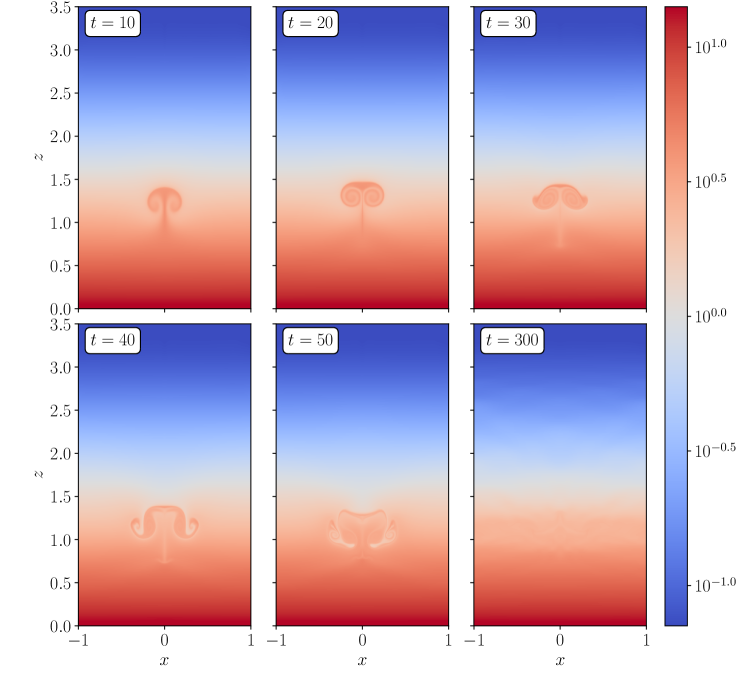
Figure 1: 2D numerical simulation of a metastable MHD atmosphere [whose properties are specified by Eq. (15)] subjected to an initial impulse of the form ${\bm{u}=u_{0}\bm{\hat{z}}\exp(-[x^{2}+(z-1.0)^{2}]/0.1^{2})}$) with $u_{0}=0.2$. This impulse is insufficient to trigger instability. The system relaxes to an final state that approximates the initial condition. The quantity visualized is the ratio of the specific entropy to the specific magnetic flux, which is conserved in a Lagrangian sense in the absence of diffusion. The physical relevance of this quantity to the phenomenon of metastability is explained in Section II. The co-ordinates $x$ and $z$ are measured in units of the total-pressure scale height and the time $t$ is measured in units of the sound-crossing time of a total-pressure scale height (see Section II.3 for details).

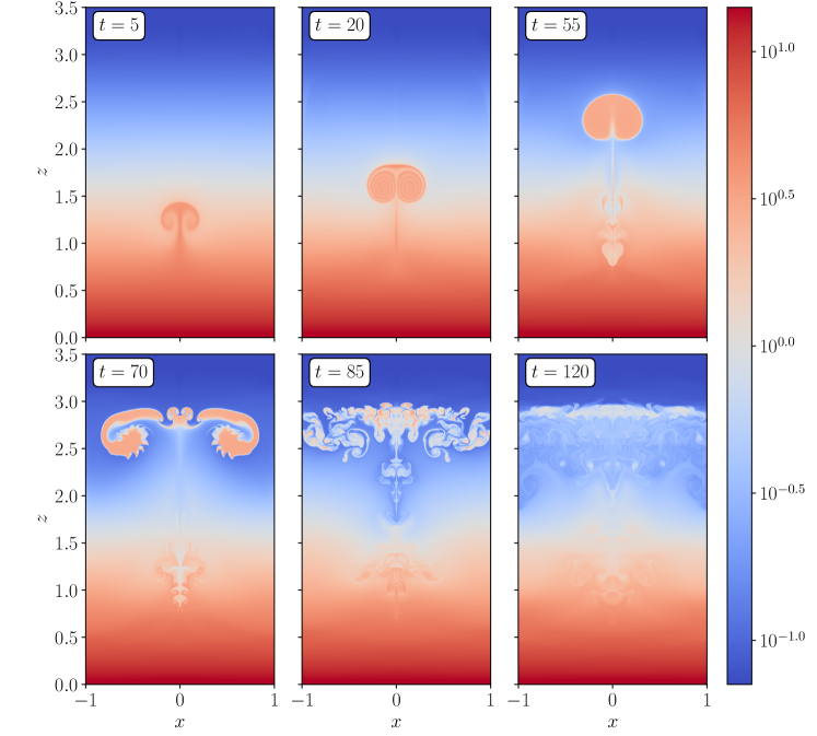
Figure 2: As Fig. 1, but for an initial velocity field that is twice as large ($u_{0}=0.4$). In this case, nonlinear instability is triggered.

These observations have motivated detailed studies of the metastability of magnetohydrodynamic (MHD) equilibria to so-called interchange or ballooning modes [5], where gradients of thermal or magnetic pressure (balanced in equilibrium by gravity or by magnetic curvature, depending on the context) provide sources of free energy for Rayleigh-Taylor instabilities that are stabilized for small (linear) perturbations, but not for large (nonlinear) ones, by field-line bending. Ref. [6] considered a stratified atmosphere with initially horizontal magnetic field embedded in conducting walls (so the endpoints of their magnetic field lines were fixed), and expanded the equations of MHD about a state of marginal linear stability in order to derive an equation of motion that retains leading-order nonlinear effects (and, therefore, metastability). In solving their equation numerically, Ref. [6] observed a phenomenon that they referred to as detonation — the progressive destabilization of the metastable equilibrium by erupting finger-like magnetic-field structures. These results were later generalized to arbitrary magnetic-field geometries with fixed end points [7] and to toroidal geometry without fixed end points [8]. Ref. [9] determined the fully nonlinear evolution of a thin elliptical erupting flux tube in the original geometry of Ref. [6], but with fast thermal conduction along field lines. In particular, they demonstrated that, depending on specific properties of the equilibrium, erupting flux tubes either find a new equilibrium position or reach a singular state with zero magnetic-field strength, a phenomenon they term flux expulsion. Ref. [10] presented schemes for determining lower-energy equilibria of individual flux tubes in toroidal geometry.

Despite the successes of these studies, the inherent geometrical complexity that arises from magnetic-field-line bending makes several key questions difficult to address, both analytically and numerically. These include: (i) To what state does a metastable equilibrium relax when it is substantially modified by a large eruption? (ii) What is the available potential energy, i.e., the difference between the energy of the initial metastable state and the global minimum of potential energy in configuration space, for a given initial configuration? (iii) Is this energy liberated in practice, i.e., is relaxation necessarily complete?

One of the main objectives of this paper is to point out that stabilization from field-line bending is not a requirement for a magnetohydrostatic equilibrium to be metastable. This is demonstrated by the numerical simulations visualized in Figs. 1 and 2, which are 2D with out-of-plane magnetic field only (we consider this case exclusively in the present paper — the in-plane component of the magnetic field is always zero in our simulations and analysis): a larger initial perturbation destabilizes the equilibrium (Fig. 2), while a smaller one does not (Fig. 1; see figure captions and Appendix A for further details).

Although it need not bend, the presence of the magnetic field is essential for metastability — in its absence, the hydrodynamic linear-stability condition (the Schwarzschild criterion [11]) guarantees nonlinear stability as well as linear. Convective stability in 2D MHD is analogous to that in moist hydrodynamics, where the metastability of terrestrial atmospheres with variable water-vapour content leads to liberation of potential energy in the form of storms (see Ref. [12] for a review). We present a general discussion of metastability in these and other analogous settings in Section II; a brief summary of the physics of metastability in the context of 2D MHD is as follows.

In 2D MHD, the dynamical role of an out-of-plane magnetic field $B$ is to provide a pressure of size $B^{2}/2$ (in appropriate units) whose effective adiabatic index is $2$ — this being greater than the adiabatic index $\gamma=5/3$ associated with thermal pressure $p$, the fluid’s compressibility $\kappa\equiv\partial\ln\rho/\partial\ln P$ is an increasing function of the ratio of thermal to magnetic pressures, $\beta\equiv 2p/B^{2}$. In other words, the density change incurred by fluid moving through a given total-pressure profile is greatest when the moving fluid is thermally dominated ($\beta\gg 1$). Now, a stratified atmosphere is linearly stable against convection if the change in the density of any fluid parcel displaced vertically by a small (linear) distance is no greater than the change in the density of the background equilibrium over the same difference in height — this ensures that the buoyancy force is restoring. In the limiting case of marginal linear stability at every height, the density gradient of the equilibrium at any given position is exactly the rate at which a fluid parcel from that position loses density with increasing height. However, this kind of equilibrium is unstable against large displacements when fluid with larger $\beta$ moves through ambient fluid with smaller $\beta$ — the density of the large-$\beta$ fluid responds more strongly to the changing pressure than the density of the background fluid does. In such cases, the buoyancy force is destabilizing. This nonlinear destabilization mechanism can persist and become dominant over large displacements even for linearly stable equilibria, provided that they are sufficiently close to marginal linear stability — those equilibria are metastable.

After Section II, the rest of our paper is concerned with the relaxation of metastable 2D MHD equilibria of the sort described above after they are destabilized. The absence of complex geometry makes certain problems tractable in 2D MHD that are difficult or impossible to solve accurately in the fully 3D case. In Section III, we address the related questions of how much potential energy is available to be liberated during non-diffusive relaxation and of what the associated minimum-energy state is. In Section III.2, we present a simple argument that indicates the available potential energy of a metastable atmosphere is always a small fraction (i.e., at most a few percent) of its total potential energy — this is confirmed by a more detailed calculation in Appendix C. The reason is that fluid parcels exclude each other: when a fluid parcel rises to the top or sinks to the bottom of an atmosphere, it prevents others from doing the same (of course, the total energy of an entire atmosphere is typically very large, so the smallness of the available-energy fraction does not present a problem for interpreting explosive energy releases in nature).

In Section III.3, we show how the (global) minimum-energy state accessible by ideal (i.e., non-diffusive) rearrangements of a general finite-$\beta$ equilibrium can be determined via a combinatorial optimization problem (linear sum assignment). Similar schemes have recently been constructed by Refs. [13, 14, 15] in the context of ocean dynamics and moist hydrodynamics in the terrestrial atmosphere. We find that the minimum-energy states typically turn out to be two dimensional over a finite range of the vertical coordinate $z$, even though we restrict consideration to initial configurations for which all quantities only depend on $z$. No constraint is imposed energetically on the scale of structures in the direction of the ignorable horizontal coordinate, $x$, so the detailed structure of the two-dimensional states during relaxation is determined dynamically — in particular, it depends on viscosity (i.e., the Reynolds number), which controls the spatial scale of flows that develop from a given initial condition. We verify with numerical simulations that, at small Reynolds number (laminar flow), metastable atmospheres do indeed relax to a state that resembles the 2D ground state.

In Section IV, we consider the relaxation of a destabilized metastable equilibrium at large Reynolds number. In that case, the potential energy liberated ends up as the kinetic energy of a turbulent flow, which mixes fluid that originates from different spatial locations — see Fig. 2. We present an equilibrium statistical mechanical theory of this sort of relaxation in Section IV.1, analogous to the Lynden-Bell [16] statistical mechanics of self-gravitating systems or collisionless plasmas, and the Robert-Sommeria-Miller (RSM) theory of 2D vortex turbulence [17, 18, 19, 20] which has found widespread application in geophysical fluid dynamics (see Ref. [21] for a recent review). In our theory, the specific entropy $s$ and magnetic flux $\chi$, each of which is conserved in a fluid-element-wise sense under non-dissipative dynamics, play the role of the phase-space density or vorticity in the Lynden-Bell or RSM theories, respectively. A summary of our treatment is as follows. Analogously to the theories described above, we define a probability-density function to find fluid with particular material properties (i.e., values of $s$ and $\chi$) at a given position in space, and determine it by maximising its associated Boltzmann mixing entropy subject to the constraints imposed by conservation laws (see Section IV.1). In the limit of zero thermodynamical temperature (which corresponds to the minimum energy the system can have), the probability distribution function becomes narrowly peaked about the solution of the assignment problem described above (see Section IV.3). By seeking the probability distribution with the same associated energy as that of the metastable state, we obtain a prediction for the state that would be reached under non-diffusive relaxation.

Of course, relaxation is never completely non-diffusive in reality — the generation of fine-scale structure in $s$ and $\chi$ by turbulent motions is always ultimately arrested by the finite thermal conductivity and/or magnetic diffusivity, even if their associated diffusion coefficients are very small (see Fig. 2). Unlike in the Lynden-Bell or RSM theories, the energy (strictly, enthalpy) density of a stratified fluid depends nonlinearly on the advected scalars $s$ and $\chi$. It follows that one cannot, as in those theories, assume that diffusion (originating from collisionality or viscosity in the Lynden-Bell and RSM theories, respectively) of the stochastic mixed state preserves the expectation values of the mixed quantities at any given position in (phase) space, as it does the expectation value of the total energy. This makes sense, physically: total magnetic flux is conserved during magnetic diffusion and heat flow, but thermal entropy is not. To account for this, we extract predicted profiles from the derived probability distribution function by assuming that diffusion preserves both magnetic flux and energy, and use these requirements to determine the profile of $s$ for the relaxed state.

A second consequence of the nonlinear dependence of the energy density on $s$ and $\chi$ is that the predicted diffused state, obtained as explained above, need not itself have zero available potential energy. Indeed, it need not even be linearly stable. The reason is that diffusion alters buoyancy: a well-known example of this is the phenomenon of “buoyancy reversal” in terrestrial atmospheres: when buoyantly rising dry air mixes with moist air, it may, after diffusion, become more dense than the unmixed moist air and sink again as a result (see, e.g., Ref. [12]). In our theory, we account for this effect with a simple expedient that is consistent with the idea of a separation in timescales between ideal mixing and diffusion — we take the predicted unstable (or metastable) diffused state to be the start point for a new chaotic relaxation, and employ the procedure outlined above to obtain a second relaxed state. If necessary, this procedure can be repeated until a stable diffused state is reached, although we find that one iteration is often enough to do so. We find that the profiles of $s$ and $\chi$ produced by this procedure are typically only slightly modified from the ones derived from the statistical mechanics in the first instance — qualitatively, we find that the subsequent rearrangements and accompanied diffusion tend to produce plateaus in the profiles of $s$ and $\chi$.

In Section V, we compare the results of our statistical mechanical treatment with those of direct numerical simulations of relaxing metastable equilibria at large Reynolds number. The agreement turns out to be reasonably good, although less so for small initial perturbations, as the system “gets stuck” in a metastable state and does not mix thoroughly. We conclude with a discussion of possible implications and applications in Section VI.

We caveat our results with the following note. As we show in Section II, a necessary criterion for a stratified equilibrium to be metastable is that either $s$ or $\chi$ decreases with height over a finite range of $z$. Depending on the relative sizes of the magnetic and thermal diffusivities, equilibria of this sort can be linearly unstable to so-called double-diffusive instabilities (see, e.g., Ref. [22], and references therein), the simplest of which is the fingering instability that occurs if the diffusivity of the quantity whose stratification is stabilizing is large, and therefore the stabilization is not felt. In this work, we shall always assume that the ratio of the diffusion coefficients is such that the fluid is stable to these diffusive instabilities (which can, in any event, be suppressed by viscosity), and choose diffusion coefficients for numerical simulations such that this is true (see Appendix A). The application of our statistical mechanical approach to double-diffusive instabilities and their saturation is a topic that we hope to explore in future work.

II Theory of convective metastability

II.1 General equation of state

Although often derived by linear-stability analysis (see, e.g.,  [23]), the Schwarzschild criterion [11]

$$\frac{\mathrm{d}s}{\mathrm{d}z}>0$$ (1)

on the dependence of the specific entropy $s$ on height $z$ for the convective stability of a fluid in mechanical equilibrium is, in fact, a criterion for nonlinear stability, as we now demonstrate. The upwards buoyancy force $F$ on a small parcel of fluid with equation of state $\rho=\rho(p,s)$ that was moved adiabatically (i.e., without heat flow) and in pressure balance with its surroundings from height $z_{1}$ to $z_{2}$, where its volume is $V_{2}$, is given by

$$F =-gV_{2}\left[\rho(p_{2},s_{1})-\rho(p_{2},s_{2})\right]$$

$$=-gV_{2}\int_{z_{2}}^{z_{1}}\mathrm{d}z\,\frac{\mathrm{d}s}{\mathrm{d}z}\,\frac{\partial\rho(p_{2},s)}{\partial s}.$$ (2)

This force is restoring (i.e, has opposite sign to that of $z_{2}-z_{1}$) even for finite $z_{2}-z_{1}$, provided that (i) $\partial\rho(p,s)/\partial s<0$, i.e., that the fluid expands under heating at constant pressure, and (ii) Eq. (1) holds for ${z\in[z_{1},z_{2}]}$ [in Eq. (2), $p$ is the thermal pressure, $g$ is the acceleration due to gravity and we use the notation $p_{2}=p(z_{2})$ etc. for equilibrium quantities].

However, the criteria for linear and nonlinear stability become distinct if the fluid density depends on additional quantities besides thermal pressure and entropy. In different contexts, such quantities could include salinity, moisture content, the entropy of a radiation field, or magnetic flux. To generalize Eq. (2) to such cases, we let $\bm{Q}$ be a vector whose components are all the relevant quantities upon which density depends, and which we assume are, like entropy, advected by the flow in the absence of diffusion. Then, Eq. (2) becomes

$$F =-gV_{2}\left[\rho(P_{2},\bm{Q}_{1})-\rho(P_{2},\bm{Q}_{2})\right]$$

$$=-gV_{2}\int^{z_{1}}_{z_{2}}\mathrm{d}z\frac{\mathrm{d}\bm{Q}}{\mathrm{d}z}\bm{\cdot}\frac{\partial\rho(P_{2},\bm{Q})}{\partial\bm{Q}}$$ (3)

where $P$ is the total pressure (including non-thermal components) — again, we have assumed that the displaced fluid parcel is always in total-pressure balance with its surroundings. The generalization of the Schwarzschild criterion (1) for linear stability is

$$\mathcal{L}\equiv-\frac{\mathrm{d}\bm{Q}}{\mathrm{d}z}\bm{\cdot}\frac{\partial\ln\rho(P,\bm{Q})}{\partial\bm{Q}}>0.$$ (4)

In many situations of interest (including the examples above), the quantities $Q_{i}$ can be chosen such that ${\partial\ln\rho(P,\bm{Q})}/{\partial Q_{i}}<0$. Evidently, in such cases, linear stability is assured if ${\mathrm{d}Q_{i}/\mathrm{d}z>0\,\,\,\forall i}$. Furthermore, by Eq. (3), such an equilibrium would also be nonlinearly stable to convection. However, while this condition is sufficient for linear stability, it is not necessary that all the $Q_{i}$ must increase upwards — if $\mathrm{d}Q_{i}/\mathrm{d}z<0$ for some $i$, the gradients of other components of $\bm{Q}$ could compensate such that Eq. (4) remained satisfied. In those cases, the equilibrium would be linearly stable, but not necessarily nonlinearly stable.

The precise conditions under which nonlinear instability (i.e., metastability) occurs may be deduced by recasting Eq. (3) as the upwards force per unit mass of moved fluid, ${F/\rho(P_{2},\bm{Q}_{1})V_{2}=(e^{\mathcal{R}}-1)g}$, where

$$\mathcal{R}\equiv\ln\frac{\rho(P_{2},\bm{Q}_{2})}{\rho(P_{2},\bm{Q}_{1})}\\ =\int^{z_{2}}_{z_{1}}\mathrm{d}z\mathcal{L}+\int^{z_{2}}_{z_{1}}\mathrm{d}z\frac{\mathrm{d}\ln P}{\mathrm{d}z}[\kappa(P,\bm{Q}_{1})-\kappa(P,\bm{Q})],$$ (5)

and we have introduced the dimensionless fluid compressibility

$$\kappa(P,\bm{Q})\equiv\frac{\partial\ln\rho(P,\bm{Q})}{\partial\ln P}.$$ (6)

The utility of Eq. (5) is that it separates the integrated linear buoyancy response (the first integral on the second line) with the nonlinear response (the second integral), revealing the latter to be determined by the path-integrated difference in $\kappa$ between the moving fluid and its surroundings. In particular, if the displaced fluid is more compressible than the fluid it moves through, i.e., $\kappa(P,\bm{Q}_{1})>\kappa(P,\bm{Q})$, then the second integral on the right-hand side of Eq. (5) has the same sign as $z_{2}-z_{1}$, so its contribution to the buoyancy force is destabilizing. If the stabilizing effect of the integral involving $\mathcal{L}$ is sufficiently small, then the second integral dominates in Eq. (5) for sufficiently large $\delta z$, so the equilibrium is metastable.

II.2 Two-dimensional magnetohydrodynamics

In the remainder of this paper, we focus on the simple case of a two-dimensional atmosphere supported against gravity both by thermal pressure $p$ and the magnetic pressure associated with an out-of-plane magnetic field $B$, i.e., ${P=p+B^{2}/2}$. The forms of the general results derived above are then as follows. The conserved quantity associated with $B$ is the specific magnetic flux, $\chi=B/\rho$, and, for symmetry with $\chi$, we take $s=p^{1/\gamma}/\rho$ (any monotonically increasing function of entropy would suffice) where $\gamma$ is the adiabatic index. Thus, we have $\bm{Q}=(s,\chi)$. With these choices, Eq. (4) yields the linear-stability condition

$$\mathcal{L}=\frac{c_{s}^{2}}{c^{2}}\frac{\mathrm{d}\ln s}{\mathrm{d}z}+\frac{v_{A}^{2}}{c^{2}}\frac{\mathrm{d}\ln\chi}{\mathrm{d}z}>0,$$ (7)

where $c_{s}\equiv\sqrt{\gamma p/\rho}$ is the sound speed, $v_{A}\equiv B/\sqrt{\rho}$ the Alfvén speed and $c=\sqrt{c_{s}^{2}+v_{A}^{2}}$ is the velocity of compressive waves [Eq. (7) is sometimes called the modified Schwarzschild criterion]. The compressibility $\kappa$ [Eq. (6)] is

$$\kappa(P,s,\chi)=\frac{1+\beta}{2+\gamma\beta},$$ (8)

where $\beta\equiv 2p/B^{2}$ is the plasma beta — the ratio of thermal to magnetic pressures — which is determined from $P$, $s$ and $\chi$ via

$$\frac{1}{\beta}\left(1+\frac{1}{\beta}\right)^{\frac{2}{\gamma}-1}=\frac{1}{2}\left(\frac{\chi}{s}\right)^{2}P^{\frac{2}{\gamma}-1}.$$ (9)

We see from Eq. (8) that $\kappa$ increases monotonically with $\beta$, from $\kappa=1/2$ at $\beta\to 0$ to $\kappa=1/\gamma$ at $\beta\to\infty$. It follows that the nonlinear buoyancy response in Eq. (5) is destabilizing when fluid with large $\beta$ moves through ambient fluid with smaller $\beta$. Because the moving and ambient fluid are in pressure balance (by assumption), Eq. (9) reveals that the nonlinear response is destabilizing when the moving fluid has a larger value of the ratio $s/\chi$ than the ambient fluid does. Thus, a 2D MHD atmosphere sufficiently close to marginal linear stability is metastable to displacements of fluid with larger values $s/\chi$ through ambient fluid with smaller values of $s/\chi$ [cf. Figs. 1 and 2]. Loosely, $s/\chi$ can be thought of as “potential $\beta$”, analogous to potential temperature in atmospheric science and ocean dynamics: by Eq. (9), it is (a monotonically increasing function of) the $\beta$ that a fluid element would have when brought to a fixed reference pressure.

II.3 Examples of metastable equilibria

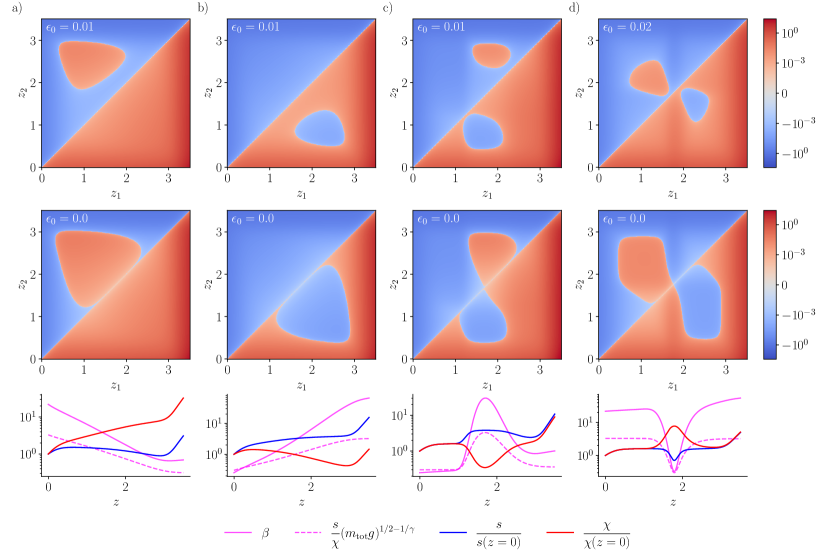
Figure 3: Top row: the upward force [Eq. (3)] per unit mass of a small fluid parcel moved in pressure balance and without diffusion from height $z_{1}$ to $z_{2}$ for each of the profiles described in Section II.3, with values of $\epsilon_{0}$ in Eq. (19) indicated on each panel. Middle row: the same as the top row, but with $\epsilon_{0}=0$ (marginal linear stability outside of the “buffer” regions). Bottom row: profiles of the specific entropy $s=p^{1/\gamma}/\rho$, specific magnetic flux $\chi=B/\rho$, their ratio, and the plasma $\beta$ [Eq. (12)] as a function of height $z$ (these profiles correspond to the top row specifically, but the profiles that correspond to the middle row look essentially the same because the differences in $\epsilon_{0}$ are very small). Panels (a) correspond to Eq. (15), Panels (b) to Eq. (16), Panels (c) to Eq. (17) and Panels (d) to Eq. (18).

We now explain how explicit examples of metastable equilibria can be obtained. It is convenient to change variables from height $z$ to the total mass supported at height $z$ (column density),

$$m=\int_{z}^{\infty}\rho(z^{\prime})\mathrm{d}z^{\prime},$$ (10)

so that the force-balance condition becomes ${P=mg}$, which may be expressed as

$$\rho^{\gamma}s^{\gamma}+\frac{1}{2}\rho^{2}\chi^{2}=mg,$$ (11)

or, equivalently, as

$$\frac{1}{\beta}\left(1+\frac{1}{\beta}\right)^{\frac{2}{\gamma}-1}=\frac{1}{2}\left(\frac{\chi}{s}\right)^{2}(mg)^{\frac{2}{\gamma}-1}.$$ (12)

Throughout this work, we shall find it convenient to use the supported mass $m$ as a proxy for height $z$ (although note that $m$ decreases with increasing $z$).

We seek an equilibrium that is close to marginal linear stability [so that the second integral in Eq. (5) stands a chance of dominating the first]. We therefore demand that

$$\mathcal{L}=\frac{\epsilon}{H_{P}},$$ (13)

where $\mathcal{L}$ is given by Eq. (7), $H_{P}$ is the total-pressure scale height $[\mathrm{d}\ln P/\mathrm{d}z]^{-1}=m/\rho$ and $\epsilon\ll 1$ is a small number. Eq. (13) constitutes a differential equation involving $s$, $\chi$ and their gradients in $m$ — to solve it, we must specify a relationship between $s$, $\chi$ and $m$ that defines the particular equilibrium under consideration. We choose to specify as a function of $m$ the ratio $s/\chi$ , which controls metastability by determining the compressibility of the fluid (see Section II.2). We therefore use Eq. (7) to recast Eq. (13) as

$$\frac{\mathrm{d}\ln s}{\mathrm{d}m}=\frac{2}{\gamma\beta+2}\frac{\mathrm{d}}{\mathrm{d}m}\ln\left(\frac{s}{\chi}\right)-\frac{\epsilon}{m}$$ (14)

and integrate Eq. (14) numerically for $s$ as a function of $m$ — we can then determine the dependence of all quantities on $m$ (or $z$) via their definitions and Eqs. (10) and (12).

Some example cases are visualized in Fig. 3, where we show $s/\chi$ and $\beta$ plotted as a functions of $z$ together with the force [Eq. (3)] per unit mass on a small parcel of fluid moved from height $z_{1}$ to $z_{2}$ as a function of $z_{1}$ and $z_{2}$: Fig. 3(a) shows

$$\frac{s}{\chi}=(m_{\mathrm{tot}}g)^{1/\gamma-1/2}\left(3\frac{m}{m_{\mathrm{tot}}}+0.3\right),$$ (15)

which increases with $m$, so the most compressible material is at the bottom of the atmosphere and the equilibrium is unstable to upwards displacements (towards larger $z$) — this is the equilibrium whose relaxation is visualized in Figs. 1 and 2; Fig. 3(b) shows

$$\frac{s}{\chi}=(m_{\mathrm{tot}}g)^{1/\gamma-1/2}\left(3\frac{m}{m_{\mathrm{tot}}}+0.3\right)^{-1},$$ (16)

which decreases with $m$, so produces an equilibrium unstable to downward displacements (towards smaller $z$); Fig. 3(c) shows

$$\frac{s}{\chi}=(m_{\mathrm{tot}}g)^{1/\gamma-1/2}\left[3\exp\left(-\frac{(m/m_{\mathrm{tot}}-0.2)^{2}}{0.1^{2}}\right)+0.3\right],$$ (17)

which has a maximum at $m=0.2m_{\mathrm{tot}}$ — the equilibrium is therefore unstable to both upwards and downwards displacements in the vicinity of the maximum; finally, Fig. 3(d) shows

$$\frac{s}{\chi}=(m_{\mathrm{tot}}g)^{1/\gamma-1/2}\times\\ \left[3\left(1-\exp\left(-\frac{(m/m_{\mathrm{tot}}-0.2)^{2}}{0.1^{2}}\right)\right)+0.3\right],$$ (18)

which has a minimum at $m=0.2m_{\mathrm{tot}}$ — more compressible fluid is therefore situated at the top and bottom of the atmosphere than in the middle, so the atmosphere is unstable to both downwards and upwards displacements.

The system of units employed in Figs. 1-3 and in the rest of the paper is as follows. We choose units of mass and length such that $\rho=1$ and ${m=m_{\mathrm{tot}}=1}$ at the bottom of the atmosphere (${z=0}$), so the total-pressure scale height $H_{P}=1$ there. We choose units of time such that $g=1$: it follows that the time taken for a compressive wave to traverse a total-pressure scale height ${H_{P}/c\sim\sqrt{H_{P}/g}=1}$ at the bottom of the atmosphere. We limit the total height of the atmospheres to $z_{\mathrm{max}}=3.5$, where $\rho\lesssim 10^{-2}$ in all cases. To stabilize the equilibria near $z=0$ and $z=z_{\mathrm{max}}$, we choose

$$\epsilon=\epsilon_{0}+\tanh\left(\frac{z-z_{u}}{\Delta_{u}}\right)-\tanh\left(\frac{z-z_{l}}{\Delta_{l}}\right)+2,$$ (19)

in Eq. (19), with $\Delta_{l}=\Delta_{u}=0.25$, $z_{l}=0.25$, $z_{u}=3.25$. The constant $\epsilon_{0}=10^{-2}$ for the simulations visualised in Figs. 1 and 2. Although we show plots that correspond to small positive values $\epsilon_{0}$ in the top row of Fig. 3, which exhibit the various sorts of metastability described above, we shall, for simplicity, focus attention on $\epsilon_{0}=0$ (i.e., the case of marginal linear stability in the bulk) in the discussion of relaxation to follow in Sections III, IV and V, unless otherwise stated. We show plots for the case of $\epsilon_{0}=0$ in the middle row of Fig. 3.

III Relaxation to the state
of minimum energy

We now turn to the subject of relaxation of metastable equilibria, which is the topic of the rest of the paper. In particular, we aim to predict the states to which metastable equilibria relax when their nonlinear instability is triggered. As when computing the force (3) on a displaced fluid parcel, let us for the moment assume that the relaxation happens at sufficiently large spatial scales and/or sufficiently short timescales that heat flow and magnetic diffusion can be neglected. It follows that $s$ and $\chi$ are conserved for each fluid element, and relaxation constitutes a rearrangement of fluid elements characterised by their conserved $s$, $\chi$ and mass. Strictly, this neglect of diffusion is only justified if the Reynolds number $\mathrm{Re}$ is small enough to prevent the development of turbulence, which would produce small-scale structures via mixing, upon which diffusion would act even with small thermal and magnetic diffusivities [generation of small-scale structure leading to diffusion is evident in the final three panels of Fig. 2]. Although we neglect it for now, we shall suggest a scheme for treating this diffusive relaxation in Section IV.5.

In this Section, we consider the problem of finding the global minimum-energy state accessible via non-diffusive rearrangement, and its properties. Provided the initial perturbation is of sufficient size and spatial extent to trigger instability throughout the atmosphere, we expect this minimum-energy state to be an attractor for the relaxation. In particular, provided that the relaxing system does not become stuck in a different local minimum, the global minimum-energy state is the end point of the relaxation of an open system (i.e., one for which the liberated potential energy can propagate out). Even for a closed system whose liberated potential energy is ultimately dissipated by viscosity to become heat, the fluid entropy need not change very much provided the available energy is small (as it does turn out to be, see Section III.2), and, again, a state approximating the global potential-energy minimum subject to ideal rearrangements ought to be reached. Finally, in the case of large $\mathrm{Re}$, where relaxation to the minimum-energy state cannot be reasonably expected, the minimum-energy state remains an object of interest, as its energy determines the available potential energy of the original equilibrium.

Because $x$ is an ignorable coordinate (i.e., one upon which the energy of a fluid parcel does not depend), we assume that the state with minimum energy is 1D, so that all quantities depend only on $z$ (or, equivalently, on supported mass $m$). It will turn out that this assumption can, and often does, fail, but the 2D minimum-energy states will be extractable from the solution to the 1D minimization problem. The total energy of a 1D equilibrium state is

$$E_{\mathrm{tot}} =\int_{0}^{\infty}\mathrm{d}z\left(\frac{p}{\gamma-1}+\frac{B^{2}}{8\pi}+\rho gz\right)$$

$$=\int_{0}^{m_{\mathrm{tot}}}\mathrm{d}m\,\mathcal{E}(m,s,\chi),$$ (20)

where, in moving to the second line we have integrated by parts, and introduced the enthalpy

$$\mathcal{E}(m,s,\chi) \equiv\frac{\gamma}{\gamma-1}\rho^{\gamma-1}s^{\gamma}+\rho\chi^{2}$$ (21)

$$=\frac{\gamma s}{\gamma-1}\left(\frac{mg}{1+1/\beta}\right)^{1-1/\gamma}\left[1+\frac{2(\gamma-1)}{\gamma\beta}\right].$$ (22)

In evaluating either of the equivalent expressions (21) or (22), $\rho$ and $\beta$ must be determined implicitly from Eqs. (11) or (12), respectively.

Following Lorenz [24], we discretize the integral (20), “slicing” the atmosphere into thin layers of equal mass $\Delta m$ that we label by the index $i$. Because the mass, entropy and flux of each fluid parcel are conserved during relaxation (by assumption), any 1D state that is accessible from the initial one can be obtained by rearrangement of the slices. We therefore seek the permutation $\sigma$ that minimises

$$E_{\mathrm{tot}}\simeq\Delta m\sum_{i=0}^{N}\mathcal{E}(m_{\sigma(i)},s_{i},\chi_{i}),$$ (23)

where $N=m_{\mathrm{tot}}/\Delta m$, and $s_{i}$, $\chi_{i}$ and $m_{i}$ are, respectively, the specific entropy and magnetic flux of, and the mass supported by, slice $i$.

The discrete energy-minimisation problem (23) has simple solutions in the limits $\beta\to\infty$ and $\beta\to 0$, i.e., the cases where only one of thermal or magnetic pressure support the atmosphere. For ${\beta\to\infty}$, ${\mathcal{E}\to\gamma s(mg)^{1-1/\gamma}/(\gamma-1)}$, so $\mathcal{E}$ increases monotonically with both $m$ and $s$, and, therefore, the arrangement with least total energy is the one for which the slice with largest $s$ has smallest $m$, the slice with the next largest $s$ has the next smallest $m$, and so on. It follows that the profile with the smallest energy is the unique rearrangement for which $s$ is a monotonically increasing function of height — indeed, we already know this state to be nonlinearly stable by Eq. (2). A similar conclusion is obtained for ${\beta\to 0}$, for which ${\mathcal{E}\to 2(mg)^{1/2}\chi}$ and so the nonlinearly stable atmosphere is the one with $\chi$ increasing monotonically with height. However, analogous simple constructions for the minimum-energy configuration do not exist in the finite-$\beta$ case — the optimal solution that balances the competing imperatives of “entropy should increase upwards” and “flux should increases upwards” is non-trivial. As illustration of this, we see from Eq. (12) that a fluid parcel with any fixed values of $s$ and $\chi$ has $\beta\to\infty$ as $m\to 0$ but $\beta\to 0$ as $m\to\infty$. It follows that, according to the stacking rules just stated, the minimum-energy state must be stacked in order of ascending $\chi$ at large $m$ but in order of ascending $s$ at small $m$: there is no global stacking rule that is valid for all $m$.

III.1 Energy minimisation as an assignment problem

The problem of finding the minimum-energy state, i.e., of minimising Eq. (20) over permutations $\sigma$, is a combinatorial optimization problem known as the Linear Sum Assignment (LSA) problem (see, e.g., Ref. [25]). The LSA problem is canonically described as one of minimising the total cost associated with assigning a number of “agents” to the same number of “tasks” — in our case, the “agents” are the slices of atmosphere with given $s$ and $\chi$, while their “tasks” are to occupy the discrete positions in the atmosphere with each possible value of the discretized supported mass. The cost associated with assigning agent $i$ to task $j$ is ${\mathcal{E}(m_{j},s_{i},\chi_{i})}$, which we can denote more efficiently as ${\mathcal{E}(m_{j},m_{i})}$: this is the energy cost associated with assigning the slice initially at supported mass $m_{i}$ to the new supported mass $m_{j}$ (in a minor abuse of notation, we use the same symbol, $\mathcal{E}$, for both quantities). Despite our discretization in $m$, ${\mathcal{E}(m_{j},m_{i})}$ remains a continuous function of its arguments, and we shall frequently be required to integrate or take derivatives with respect to one or the other. We shall, therefore, introduce the continuous variable $\mu$ to denote the supported mass of a slice in the initial state, and denote the continuous form of ${\mathcal{E}(m_{j},m_{i})}$ by $\mathcal{E}(m,\mu)\equiv\mathcal{E}(m,s(\mu),\chi(\mu))$ in what follows. In a similar manner, we shall write $\rho(m,\mu)$ as a shorthand for $\rho(P=mg,s(\mu),\chi(\mu))$. We note for later use that, according to Eqs. (11) and (21),

$$\frac{\partial\mathcal{E}(m,\mu)}{\partial m}=\frac{g}{\rho(m,\mu)}.$$ (24)

A useful observation is that the modified cost matrix $\tilde{\mathcal{E}}(m_{j},m_{i})$, where

$$\tilde{\mathcal{E}}(m_{j},m_{i})=\mathcal{E}(m_{j},m_{i})-a(m_{j})-b(m_{i}),$$ (25)

has the same optimal assignment of agents to tasks as does the original cost matrix ${\mathcal{E}(m_{j},m_{i})}$. This is intuitive: if the cost of assigning a given agent to each task decreases by the same amount, their optimal assignment will not change (although the total cost of the solution will decrease); likewise, if a particular task becomes more expensive by the same amount for all agents, the optimal choice of agent for that task will remain the same. $\tilde{\mathcal{E}}$ is called the “normal form” of the cost matrix $\mathcal{E}$ if it satisfies the following properties [25]:

1. $\tilde{\mathcal{E}}(m_{j},m_{i})\geq 0$,

2. There exists at least one bijection $\sigma$ such that $\tilde{\mathcal{E}}(m_{\sigma(i)},m_{i})=0,\,\,\,\forall i$.

A proof that an $\tilde{\mathcal{E}}(m_{j},m_{i})$ with these properties can always be found with suitable choices of $a(m_{j})$ and $b(m_{i})$ is provided by the “Hungarian algorithm” [26, 27], which consists of a series of row and column operations on the cost matrix that are guaranteed to reduce it to normal form in polynomial (in $N$) time. The utility of the normal form $\tilde{\mathcal{E}}(m_{j},m_{i})$ is that each of the bijections $\sigma$ constitutes an optimal assignment [typically, the optimal assignment is unique — this is true for each of the equilibria introduced in Section II.3 (see Section III.3), but is not always the case: the optimal assignment is non-unique when multiple slices have the same values of $s$ and $\chi$].

III.2 Available energy is small: $E_{\mathrm{avail}}\ll E_{0}$

Before reporting the results of the energy minimization for the metastable equilibria described in Section II.3, we first present a simple argument that indicates the available potential energy of a metastable atmosphere is always a small fraction of its total potential energy. Let us consider the change in potential energy $\delta E$ that results from moving a slice of atmosphere upwards from supported mass $m_{a}$ to new supported mass $m_{b}$, shuffling downwards the slices that it passes on the way. By Eq. (24), this is

$$\frac{\delta E}{\Delta m} =\mathcal{E}(m_{b},m_{a})-\mathcal{E}(m_{a},m_{a})$$

$$\quad+\sum_{i=b}^{a-1}\left[\mathcal{E}(m_{i+1},s_{i},\chi_{i})-\mathcal{E}(m_{i},s_{i},\chi_{i})\right]$$

$$\simeq\int^{m_{b}}_{m_{a}}\mathrm{d}m\left[\frac{g}{\rho(m,m_{a})}-\frac{g}{\rho(m,m)}\right]$$

$$=-g\int^{z_{a}}_{z_{b}}\mathrm{d}z\left[\frac{\rho(m(z),m(z))}{\rho(m(z),m_{a})}-1\right],$$ (26)

where $m(z_{a})=m_{a}$, and likewise for $b$. The integrand that appears in the last line of Eq. (26) is straightforwardly recognized as the net buoyancy force (3) per unit mass of fluid, so, sensibly, $\delta E$ is just the work done by this force on the moving slice. Evidently, the energy that can be liberated by this process is maximal when the ratio that appears inside the integrand in the last line of Eq. (26) — i.e., of the density of the ambient fluid to the density of the slice — is maximal. We can evaluate this ratio using Eq. (5), which yields, in the most optimistic case of (i) marginal linear stability, i.e., $\mathcal{L}=0$, (ii) $\kappa=1/\gamma$ inside the slice (maximally compressible large-$\beta$ fluid) and (iii) $\kappa=1/2$ for the ambient fluid (minimally compressible small-$\beta$ fluid),

$$\frac{\rho(m,m_{a})}{\rho(m,m)}=\left(\frac{m}{m_{a}}\right)^{1/\gamma-1/2}.$$ (27)

Substituting this into Eq. (26), choosing $m_{a}=m_{\mathrm{tot}}$ (the slice originates from the bottom of the atmosphere) and evaluating integrals, we find that

$$\frac{\delta E}{\Delta m}=\frac{3}{4}\frac{E_{0}}{m_{\mathrm{tot}}}\left[\frac{\gamma}{\gamma-1}\left(\left(\frac{m_{b}}{m_{\mathrm{tot}}}\right)^{1-1/\gamma}-1\right)\right.\\ \left.-2\left(\left(\frac{m_{b}}{m_{\mathrm{tot}}}\right)^{1/2}-1\right)\right],$$ (28)

where $E_{0}$ is the initial total energy of the atmosphere [assuming that it is mostly populated with small-$\beta$ fluid, as is consistent with assumption (iii) above]. In the limit $m_{b}/m_{\mathrm{tot}}\to 0$ and with $\gamma=5/3$, Eq. (28) yields ${\delta E/{E_{0}}\simeq-3\Delta m/8m_{\mathrm{tot}}\sim-\Delta m/m_{\mathrm{tot}}}$. The liberation of potential energy when a single slice rises to the very top of the atmosphere is therefore efficient — if a similarly favorable scaling applied to the reassignment of a mass ${\sim m_{\mathrm{tot}}}$ of fluid, then we would expect order-unity fractional available energy. However, most slices are not reassigned to the very top of the atmosphere in practice: at most, a mass $\delta m$ of fluid can be reassigned to $m<\delta m$. For the vast majority of slices, the supported mass at their reassigned position is a finite fraction of their supported mass in the initial state. With, for example, $m_{b}=m_{\mathrm{tot}}/2$, Eq. (28) yields ${\delta E/{E_{0}}\simeq-0.015\Delta m/m_{\mathrm{tot}}\sim-10^{-2}\Delta m/m_{\mathrm{tot}}}$. Thus, typical reassignments are far less profitable — this is because they do not cause a slice to experience a large change in total pressure. A more detailed calculation (see Appendix C) reveals that $10^{-2}$ is indeed a good estimate for the fractional available energy — the maximum fractional available energy of a (marginally) stable atmosphere consisting of small-$\beta$ fluid above a layer of large-$\beta$ fluid is $1.75\%$. We shall find that the fractional available energies of the equilibria described in Section II.3 and represented in Fig. 3 is less than this (by roughly an order of magnitude), owing to the facts that (i) these equilibria have finite $\beta$, and thus do not have the extremal values of the fluid compressibility considered here; and (ii) the stable buffer regions contribute to the potential energy of the equilibrium (and prevent the relaxing fluid from accessing large pressure differences) but do not participate in the reassignment.

III.3 Energy minimization: numerical results
and interpretation

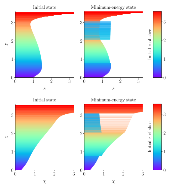
Figure 4: Visualisation of the assignment of 1D slices that minimizes the total energy, Eq. (23), with $\Delta m=5\times 10^{-4}m_{\mathrm{tot}}$, for the upwards-unstable profile defined by Eq. (15). Panels on the left show the initial profiles of $s$ and $\chi$ as functions of height $z$, while panels on the right show the minimum-energy assignment. The slices are colored by their height $z$ in the initial state to aid comparison. Each slice has vertical extent $\Delta z=\Delta m/\rho$ with $\rho$ given by Eq. (11).

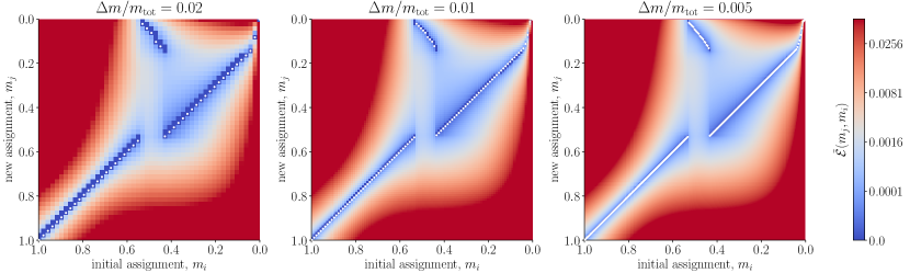
Figure 5: The normal form of the cost matrix $\tilde{\mathcal{E}}(m_{j},m_{i})$ [Eq. (25)] for the unstable-upwards profile defined by Eq. (15), for three different choices of the discretization scale $\Delta m$.

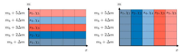
Figure 6: Visualization of the 2D restacking of Eq. (32). The left panel represents the foliated state that minimizes the potential energy (23) under 1D reassignment, while the right panel depicts a 2D state with the same energy.

In this Section, we present the outcomes of energy minimization via the Hungarian algorithm as described in Section III.1 for the metastable equilibria discussed in Section II.3 and represented in Fig. 3.

III.3.1 Metastable upwards, Eq. (15)

We first consider the equilibrium defined by Eq. (15). The solution of the LSA problem is visualized in Fig. 4, which compares the initial and minimum-energy assignments of slices. In the minimum-energy assignment, material initially from the bottom of the metastable part of the atmosphere [i.e., $z\gtrsim z_{l}$; see Eq. (19)] is reassigned to the top $z\lesssim z_{u}$, as is intuitive for an equilibrium that was nonlinearly unstable to upward displacements [see Fig. 3(a)]. The stacking order of the slices that are re-assigned also reverses — the reason is that, because the material moves to smaller $m$, its $\beta$ increases [by Eq. (12)], and therefore the contribution of $s$ to the linear stability criterion becomes more important relative to $\chi$. As a consequence, the stacking order reverses in order for $s$ to be increasing upwards.

A striking feature of the minimum-energy state is that there is no interface between the slices reassigned from the bottom of the atmosphere and the slices from the top. Instead, the fluid from the bottom forms foliated layers with the fluid from the top. The scale of the foliation is set by $\Delta m$, and therefore is arbitrarily small as $\Delta m\to 0$ — this is illustrated by Fig. 5, which shows, for three different values of $\Delta m$, the normal-form cost matrix $\tilde{\mathcal{E}}(m_{j},m_{i})$, with its zeros [which indicate the optimal assignment $j=\sigma(i)$] marked with white circles. Because the scale of foliation depends on $\Delta m$, the optimal assignment of slices does not converge as $\Delta m\to 0$, although it does converge in a coarse-grained sense: the proportion of slices assigned to any small finite range of $m$ that originated from any similarly small given range of $\mu$ converges as $\Delta m\to 0$ (provided that $\tilde{\mathcal{E}}$ converges as $\Delta m\to 0$). This must be true because, in the continuous limit, these proportions can be determined from the gradient of the locus of points for which $\tilde{\mathcal{E}}=0$. For example, denoting this locus, i.e., the curve to which the white circles in Fig. 5 converge as $\Delta m\to 0$, by $m_{\mathrm{opt}}(\mu)$, then, provided $m_{\mathrm{opt}}(\mu)$ is single valued (as is the case for the profile under consideration, see Fig. 5), the proportion of slices assigned to the vicinity of $m_{2}$ that originally had supported mass $m_{1}$ is $|\mathrm{d}m_{\mathrm{opt}}/\mathrm{d}\mu|$ evaluated at $m_{1}$ (by the conservation of mass). In the absence of foliation, ${|\mathrm{d}m_{\mathrm{opt}}/\mathrm{d}\mu|^{-1}=1}$, but, where there is foliation, it must be the case that ${|\mathrm{d}m_{\mathrm{opt}}/\mathrm{d}\mu|>1}$, so $m_{\mathrm{opt}}(\mu)$ steepens. Both cases may be observed in Fig. 5. The generalisation to the case where $m_{\mathrm{opt}}$ is multi-valued somewhat more complex, but it remains true in that case that the fractional assignments are determined by gradients of the optimal-solution curve [see Section IV.4 and Appendix F].

We can develop some intuition for the foliation phenomenon with an analogous calculation to the one in Section III.2. We again consider forming a new equilibrium state by moving a slice of atmosphere upwards from its initial assignment at $m_{a}$ to $m_{b}$, displacing downwards the slices through which it passes. The energy has a local minimum as a function of displacement of the slice when its density in its new location $\rho(m_{b},m_{a})$ is equal to the density $\rho(m_{b},m_{b})$ of the slices that surround it (neutral buoyancy), as this makes the integrand in the second line of Eq. (30) zero at $m=m_{b}$ (intuitively, if the densities were different, the new equilibrium would be Rayleigh-Taylor unstable either at the upper or lower surface of the slice). Now let us consider a second slice of fluid that initially neighbors the first, i.e., that originates from supported mass $m_{a}+\Delta m$. This slice reaches neutral buoyancy at a different supported mass $m_{b}+\delta m$. If the density of the background equilibrium changes more slowly with supported mass at $m_{b}$ than at $m_{a}$, then $\delta m>\Delta m$. Setting the density of the second slice, ${\color[rgb]{0,0,0}\rho(m_{b}+\delta m,m_{a}+\Delta m)}$, equal to that of the ambient fluid at supported mass $m_{b}+\delta m$, i.e., ${\rho(m_{b}+\delta m,m_{b}+\delta m)}$ (because we are concerned with the motion of only two slices of infinitesimal thickness, we neglect the fact that the reassignment of the first slice might have changed the identity of the fluid at $m_{b}$), we discover that

$${\color[rgb]{0,0,0}\cfrac{\delta m}{\Delta m}={\cfrac{\partial\rho(m_{b},\mu)}{\partial\mu}\bigg{|}_{\mu=m_{a}}\Bigg{/}\cfrac{\partial\rho(m_{b},\mu)}{\partial\mu}\bigg{|}_{\mu=m_{b}}}},$$ (29)

which tells us that the adjacency of the slices is not preserved under reassignment, even though they become arbitrarily close together as $\Delta m\to 0$.

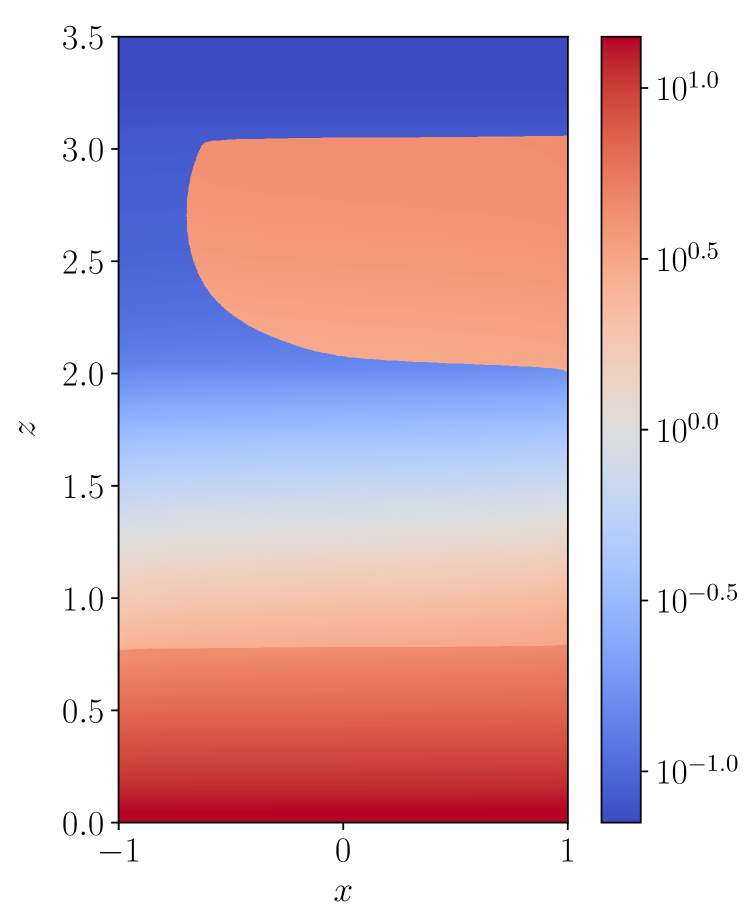
Figure 7: Visualization of $s/\chi$ for a 2D minimum-energy state of the unstable-upwards profile defined by Eq. (15). We calculate this state using Eq. (40) with $\beta_{T}=10^{6}$ (see Section IV.4).

Although Eq. (29) reveals the physical reason for foliation, it evidently fails if the fraction on the right-hand side is small: $\delta m\lesssim\Delta m$ is not allowed for the discrete problem because slices exclude each other. It also does not apply in the case where a substantial mass of fluid is reassigned, in which case the background equilibrium through which the first slice moves is different from that through which the last slice does. We can handle these cases as follows. Let us suppose that we are somehow given all the optimal assignments $\sigma(i)$, except those to some small range of $m$, i.e., those with $m_{\sigma(i)}=m_{b}+\delta m_{\sigma(i)}$, and seek the condition for which the optimal choice of the remaining assignments will be a foliated state. The contribution to the total energy of the slices that remain to be assigned is

$$\delta E =\Delta m\sum_{i}\mathcal{E}(m_{b}+\delta m_{\sigma(i)},m_{i})$$

$$=\Delta m\sum_{i}\bigg{[}\mathcal{E}(m_{b},m_{i})+\frac{\delta m_{\sigma(i)}g}{\rho(m_{b},m_{i})}+\mathcal{O}(\delta m_{\sigma(i)}^{2})\bigg{]},$$ (30)

where sums are over all indices $i$ of the slices that remain to be assigned, and we have used Eq. (24) to obtain the second equality. The first term inside the square bracket in the second line of Eq. (30) is independent of the assignment $\sigma$. The second term takes the form of the differential supported mass $\delta m_{\sigma(i)}$ multiplied by a quantity that does not depend on $\sigma(i)$, viz., $1/{\rho(m_{b},m_{i})}$. This yields a local sorting rule for the minimization of $\delta E$ — it is minimized when the slice with largest $\rho(m_{b},m_{i})$ is assigned to the largest supported mass within the small range under consideration, the next largest $\rho(m_{b},m_{i})$ is assigned to the next largest supported mass, and so on. The physical interpretation is the same as before — if more-dense slices were situated above less-dense ones, the equilibrium would be Rayleigh-Taylor unstable. Slices $i$ and $i^{\prime}$ that were non-neighboring in the original configuration typically have different densities when assigned to $m_{b}$, i.e., ${\rho(m_{b},m_{i^{\prime}})-\rho(m_{b},m_{i})=\mathcal{O}(\Delta m^{0})}$ in general. Initially neighboring slices $i$ and ${i+1}$, on the other hand, have ${1/\rho(m_{b},m_{i+1})-1/\rho(m_{b},m_{i})=\mathcal{O}(\Delta m)}$ (provided $s$ and $\chi$ are continuous functions of $m$ in the initial profile). It follows that, in the general case, slices that were neighboring initially remain neighbors in the optimal assignment, with interfaces between two slices that were not neighboring initially being discrete, rather than foliated (see the interface at $z\simeq 0.8$ in Fig. 4). However, if the difference in the density between initially non-neighboring slices assigned to the vicinity of $m_{b}$ is small, i.e.,

$$\rho(m_{b},m_{i^{\prime}})-\rho(m_{b},m_{i})=\mathcal{O}(\Delta m),$$ (31)

then the interface will not be discrete: the optimal assignment will foliate slices that were non-neighboring initially. As $\Delta m\to 0$, we see from Eq. (31) that slices may be foliated in the vicinity of some $m$ only if they have the same density at that $m$.

The conclusion that the foliated slices in the minimum-energy state have the same density as $\Delta m\to 0$ enables an interpretation of foliation as the 1D representation of a minimum-energy state that is, in fact, two dimensional. To see that this is the case, we consider $N$ (possibly foliated) slices that that are adjacent in the minimum-energy assignment, where $n$ is a number of order unity (left panel of Fig. 6). We divide these slices into $n$ sections of equal width and rearrange them such that variation in $s$ and $\chi$ is now horizontal, rather than vertical (right panel of Fig. 6). If, as in the left panel of Fig. 6, the original state was foliated, then this operation creates a locally 2D stacking whose horizontal fractional extents are the same as the fractional abundances of the slices in the foliated 1D solution. We note that, by Eq. (31), the densities of the foliated slices are the same to leading order in $\Delta m$, which means that slices that are horizontally adjacent in $m$ space are also horizontally adjacent in real ($z$) space. The energy of the 2D state is

$$\delta E_{2D} =\frac{\Delta m}{n}\sum_{i,j}\mathcal{E}(m_{b}+i\Delta m,m_{j})$$

$$=\frac{\Delta m}{n}\sum_{i,j}\left[\mathcal{E}(m_{b},m_{j})+\frac{i\Delta m\,g}{\rho(m_{b},m_{j})}+\mathcal{O}(\Delta m^{2})\right]$$

$$={\Delta m}\sum_{j}\left[\mathcal{E}(m_{b},m_{j})+\frac{j\Delta m\,g}{\rho(m_{b},m_{j})}+\mathcal{O}(\Delta m^{2})\right]$$

$$=\delta E_{1D}+\mathcal{O}(n\Delta m^{2})$$ (32)

where $\delta E_{1D}=\Delta m\sum_{j}\mathcal{E}(m_{b}+j\Delta m,m_{j})$ is the energy of the 1D state. In moving from the second to the third line in Eq. (32), we have used that ${\rho(m_{b},m_{j})=\rho(m_{b},m_{i})+\mathcal{O}(\Delta m)}$ by Eq. (31), relabelled indices $i\leftrightarrow j$ in the second term and then summed over $i$. We see from Eq. (32) that the 2D restacking depicted in Fig. 6 changes the potential energy of the mass $n\Delta m$ of the fluid under consideration by an amount that is $\mathcal{O}(n\Delta m^{2})$ as $\Delta m\to 0$. Applying such a restacking everywhere in the atmosphere, i.e., $m_{\mathrm{tot}}/n\Delta m$ times, would change the total energy by an amount ${m_{\mathrm{tot}}/n\Delta m\times\mathcal{O}(n\Delta m^{2})=\mathcal{O}(\Delta m)}$, which vanishes as $\Delta m\to 0$. The minimum-energy state can therefore be considered to be 2D in the continuous limit. One possible 2D ground state for the equilibrium represented by Eq. (15) is shown in Fig. 7 — the method by which we obtain it is explained in Section IV.4.

The 2D minimum-energy state is not unique, as any horizontal rearrangement of the segments in the right panel of Fig. 6 or of the fluid visualized in Fig. 7 has equal energy. Energy minimization imposes no constraint on the horizontal scale, and therefore the precise 2D state reached by an atmosphere relaxing to its minimum-energy state will depend on the details of the dynamics that take it there. One mechanism by which a 2D state may develop is Rayleigh-Taylor instability: we have already remarked that foliation is the result of sorting locally by density the relaxed state of the unstable equilibrium — if slices are not sorted by density but instead form an unfoliated equilibrium state, they will have an interface that is Rayleigh-Taylor unstable. The growth rate of the Rayleigh-Taylor instability being fastest for the smallest-scale modes, 2D states with fine-scale structure will be preferred, possibly leading to diffusion and subsequent return to a 1D state. This was the fate of the simulation visualized in Fig. 2 — small-scale Rayleigh-Taylor filaments formed at $t=70$ (lower-left panel), which led to the development of 2D structure at $t=85$ (lower-center), which ultimately was diffused to produce an (approximately) 1D state by $t=120$ (lower-right). At small Reynolds number, the Rayleigh-Taylor instability develops at large scales. In that case, a 2D state should persist — we confirm this prediction with a numerical simulation in Section III.4.

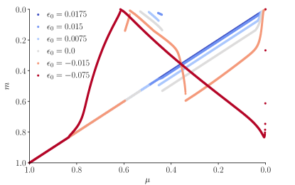
Figure 8: Minimum-energy assignments for the initial profile (15) with different values of the parameter $\epsilon_{0}$, which controls linear stability via Eq. (19).

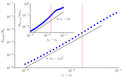
Figure 9: The available energy $E_{\mathrm{avail}}$ as a fraction of the initial potential energy $E_{0}$, plotted as a function of $\epsilon_{c}-\epsilon_{0}$, where $\epsilon_{c}\simeq 1.7\times 10^{-2}$ is the largest value of $\epsilon_{0}$ in Eq. (19) for which the initial state is metastable. The inset shows the fraction of fluid that is assigned to a smaller supported mass than its initial one under optimal reassignment. Red lines correspond to $\epsilon_{0}=0$.

To conclude our discussion of minimum-energy states of equilibria that satisfy Eq. (15), we present in Fig. 8 a comparison of energy-minimizing assignments for different values of the parameter $\epsilon_{0}$, which controls the distance from marginal stability [see Eq. (19)]. First, we note that $\epsilon_{0}=0$, i.e., marginal linear stability, is not a special point as far as the minimum-energy assignments are concerned — the assignments with $\epsilon_{0}=0.0075$ (stable), $\epsilon_{0}=0.0$ (marginal) and $\epsilon_{0}=-0.015$ (unstable) are qualitatively similar, although, in the unstable cases of $\epsilon_{0}=-0.015$ and $\epsilon_{0}=-0.075$, foliation occurs over a much wider range of supported masses (and material from three different initial locations are foliated together near the top of the atmosphere).

Fig. 9 shows the fractional energy liberated from the atmosphere, $E_{\mathrm{avail}}/E_{0}$, as a function of $\epsilon_{c}-\epsilon_{0}$, where $\epsilon_{c}\simeq 1.7\times 10^{-2}$ is the largest value of $\epsilon_{0}$ for which the atmsophere is metastable, i.e., has a restacking with smaller energy. We see that $E_{\mathrm{avail}}/E_{0}$ is small — around $10^{-3}$ for $\epsilon_{0}=0$, which is the value corresponding to Figs. 4 and 5. This is despite the fact that the minimum-energy assignment involves significant rearrangement of the atmosphere (around $10\%$ by mass of the atmosphere is reassigned upwards for $\epsilon_{0}=10^{-3}$ — see inset to Fig. 9). As explained in Section III.2, the reason for the smallness of $E_{\mathrm{avail}}/E_{0}$ is the fact that fluid slices exclude each other and so only very few of them can experience a significant change in total pressure as a result of reassignment. On the other hand, because the foliated minimum-energy assignments can involve “mixing” fluid elements with very different values for $s$ and $\chi$ at, in principle, arbitrarily small scales, significantly more potential energy may be liberated by diffusion. This is a topic to which we return in Section IV.5.

We observe from Fig. 9 that

$$\frac{E_{\mathrm{avail}}}{E_{0}}\propto(\epsilon_{c}-\epsilon_{0})^{2}\,\,\,\mathrm{as}\,\,\epsilon_{c}-\epsilon_{0}\to 0;\;$$ (33)

this scaling is readily interpreted as a result of the fact that both (i) the typical amount of energy liberated when a slice is reassigned from the bottom of the atmosphere to the top, and (ii) the number of slices that are reassigned in this way, are proportional to $\epsilon_{c}-\epsilon_{0}$ when the latter is small [see inset to Fig. 9; $s$, $\chi$ and, therefore, the buoyancy force on a displaced fluid element, Eq. (3), depend linearly on $\epsilon_{0}$, by Eq. (14)]. This argument being independent of the particular profile under consideration, we expect the dependence of $E_{\mathrm{avail}}/E_{0}$ on $\epsilon_{c}-\epsilon_{0}$ to be qualitatively similar to Fig. 8 for any metastable profile close to the critical value of $\epsilon_{0}$ for nonlinear instability; we shall find in Section III.3.2 that a similar quadratic scaling is reproduced for the profile represented by Eq. (16).

III.3.2 Metastable downwards, Eq. (16)

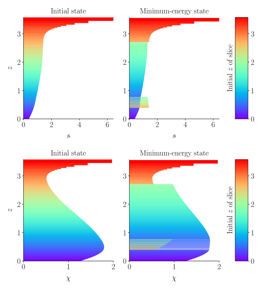
Figure 10: Visualization of the minimum-energy assignment for the equilibrium defined by Eq. (16), with $\epsilon_{0}=0$ in Eq. (19). Details are the same as for Fig. 4.

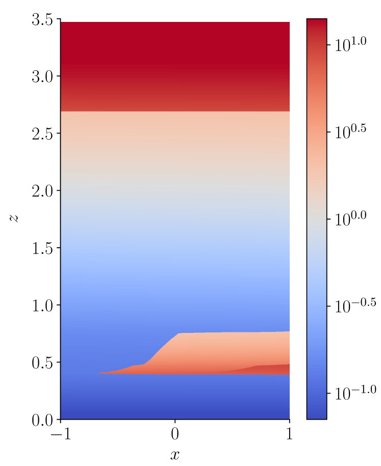
Figure 11: The ratio $s/\chi$ visualized for a 2D minimum-energy state of the unstable-downwards profile defined by Eq. (16). We calculate this state using Eq. (40) with $\beta_{T}=10^{7}$ (see Section IV.4).

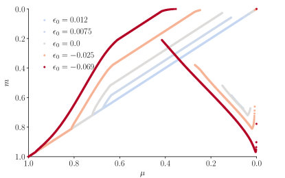
Figure 12: Minimum-energy assignments for the profile (16). We observe that the optimal assignment is one to two over certain ranges of $m_{1}$ in the cases with $\epsilon_{0}<0$.

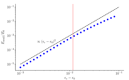
Figure 13: Fractional available energy as a function of $\epsilon_{c}-\epsilon_{0}$ for the profile (16), where $\epsilon_{c}=1.2\times 10^{-2}$ is the largest value of $\epsilon_{0}$ in Eq. (19) for which the equilibrium is metastable.

We now turn to the second case introduced in Section II, Eq. (16), which describes an initial state that is nonlinearly unstable to downwards displacements. The result of solving the LSA problem for this profile is shown Fig. 10, which is the analogue for Eq. (16) of Fig. 4. The minimum-energy assignment is similar qualitatively to the one examined in Section III.3.1 — in this case, material from the top of the atmosphere moves to the bottom, reverses stacking order, and becomes foliated with the material already there (in fact, close inspection reveals that material from three different initial heights becomes foliated over a certain range of $z$). A 2D state to which the foliated state displayed in Fig. 10 is equivalent is visualized in Fig. 11 — again, this 2D state is not unique, as horizontal rearrangements do not change the energy.

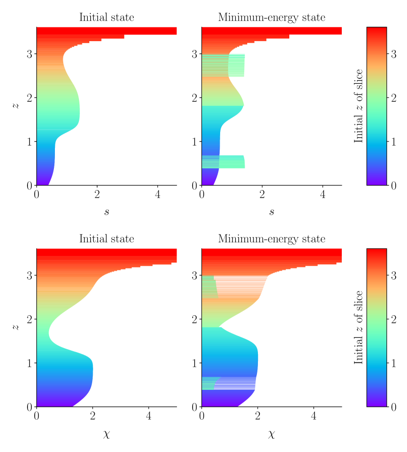
Figure 14: Visualization of the minimum-energy assignment for the equilibrium defined by Eq. (17), with $\epsilon_{0}=0$ in Eq. (19). Details are the same as for Fig. 4.

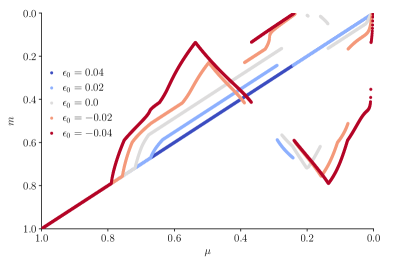
Figure 15: Minimum-energy assignments for the profile (17) for different values of $\epsilon_{0}$ in Eq. (19).

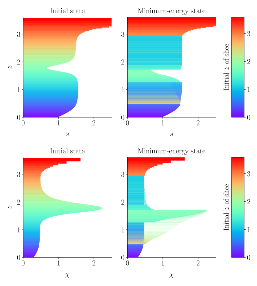
Figure 16: Visualization of the minimum-energy assignment for the equilibrium defined by Eq. (18), with $\epsilon_{0}=0$ in Eq. (19). Details are the same as for Fig. 4.

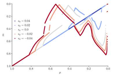
Figure 17: Minimum-energy assignments for the profile (18) for different values of $\epsilon_{0}$ in Eq. (19).

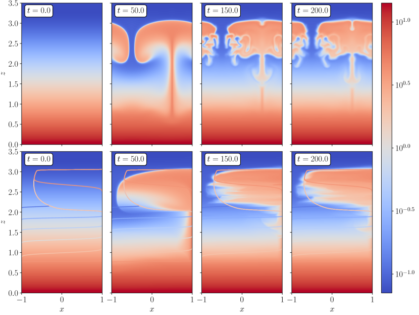
Figure 18: The relaxation of the equilibrium defined by Eq. (15) at $\mathrm{Re}\sim 10^{2}$. The intial velocity field is given by Eq. (34). Upper panels show the evolution of the ratio $s/\chi$ in $x$-$z$ space. Lower panels show the same quantity but sorted horizontally at each $z$, with contours of the theoretical minimum-energy state [Fig. 7] overlaid.

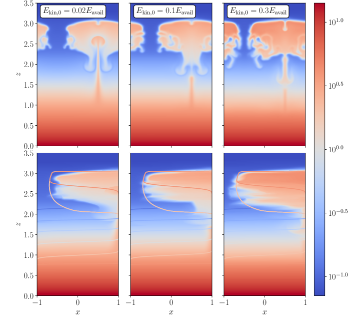
Figure 19: The distribution of $s/\chi$ at $t=300$ for simulations analogous to the one visualized in Fig. 18 but for three different values of $u_{0}$ in Eq. (34), corresponding to initial kinetic energies that are $\simeq 1/16$, $\simeq 1/4$ and $\simeq$ the available potential energy (left to right). As in Fig. 18, upper panels visualize the state of the simulation, while lower panels are sorted horizontally and overlaid with the 2D minimum-energy state [Fig. 7].

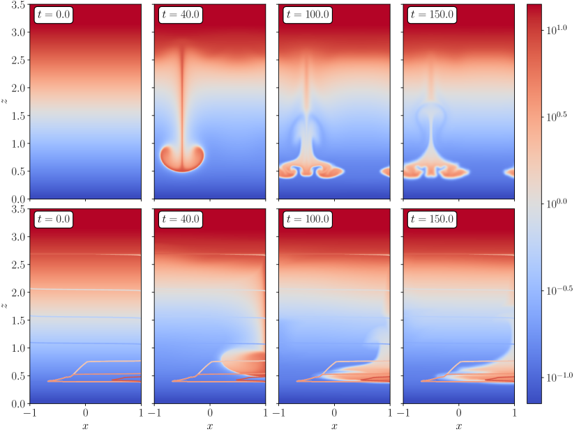
Figure 20: As for Fig. 18, but for the equilibrium defined by Eq. (16).

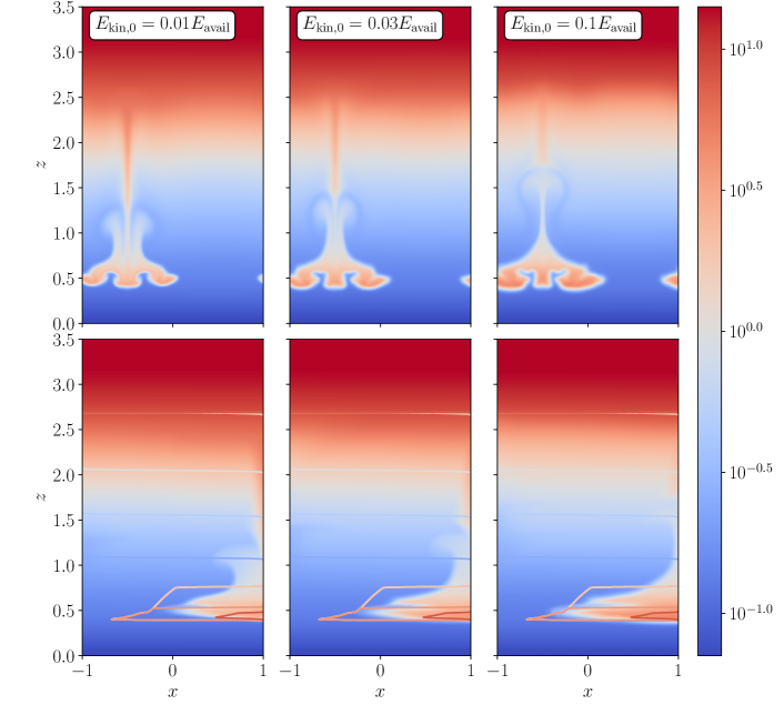
Figure 21: As for Fig. 19, but for the equilibrium defined by Eq. (16).

Fig. 13 shows the dependence of the optimal assignment on $\epsilon_{0}$ [Eq. (19)]. A qualitatively new feature appears in the cases of ${\epsilon_{0}=-0.025}$ and ${\epsilon_{0}=-0.069}$: for these unstable equilibria, there exists a range of the initial supported mass coordinate (in the vicinity of $\mu\simeq 0.25$ for the former case and $\mu\simeq 0.4$ for the latter) for which slices that are neighboring in the initial state are alternately assigned to two different final locations. Like foliation, this phenomenon can be interpreted as a consequence of our seeking a 1D optimization when, in fact, the true optimal assignment is higher-dimensional in the continuous limit $\Delta m\to 0$. In this case, the optimal assignment involves splitting the fluid at given height in a horizontal sense, and reassigning it to multiple new locations. Like metastability, this phenomenon may be understood as a consequence of the fact that the dependence of density on pressure is different depending on the composition of the fluid — this kind of “one-to-many” [in fact, we prove in Appendix D that “two” is the largest possible value of “many”] optimal assignment cannot occur over only a small range of pressure, because in that case we know from Eq. (30) that energy is minimized when slices are stacked in order of density.

III.3.3 Bi-directional metastability, Eq. (17)

We visualize in Fig. 14 the optimal assignment for the profile defined by Eq. (17), which has a local maximum in its profile of $s/\chi$ at $z\simeq 1.75$ [see Panel (c) of Fig. 3] and therefore the fluid is unstable both to upward and downward displacements there. It is intuitive, therefore, that the minimum-energy state should be obtained by reassignment of slices from the vicinity of $z\simeq 1.75$ to both the top and the bottom of the region that is close to marginal linear stability — this is indeed what we observe in Fig. 14.

Fig. 15 shows the optimal assignments for different values of $\epsilon_{0}$. The available energy associated with this profile is $6\times 10^{-4}$ of the initial total at $\epsilon_{0}=0$, which is comparable with the equilibria considered in Sections III.3.1 and III.3.2.

III.3.4 Overturning metastability, Eq. (18)

In Fig. 16, we visualize the optimal assignment for the profile defined by Eq. (18), which, in contrast to Eq. (17), has a local minimum in its profile of $s/\chi$ at $z\simeq 1.75$ [see Panel (d) of Fig. 3]. The fluid at the top of the atmosphere is therefore nonlinearly unstable to downwards motions, while the fluid at the bottom is nonlinearly unstable to upwards motions — we expect therefore that the minimum-energy state will be reached by an “overturning” of the atmosphere. This is roughly what we observe in Fig. 16, although the precise optimal assignment is remarkably complex [see Fig. (17) for a visualization of the optimal assignments in for different values of $\epsilon_{0}$]. The available energy associated with this profile at $\epsilon_{0}=0$ is $2\times 10^{-3}$ of the initial total, which is somewhat more than that of the equilibria considered in Sections III.3.1, III.3.2 and III.3.3.

III.4 Simulations of relaxation at small Reynolds number

As remarked in Section III.3.1, the 2D minimum-energy states (see Figs. 7 and 11) are likely only to be realizable in practice at small $\mathrm{Re}$, where suppression of small-scale Rayleigh-Taylor instability means that the 2D structures that develop during relaxation will be at sufficiently large scales to make thermal conduction and magnetic diffusion negligible. In this section, we present numerical simulations to verify that this is indeed the case. At small $\mathrm{Re}$, the available energy that is liberated to drive flows is readily dissipated by viscosity, and, owing to the fact that the available energy is always a small fraction of the total potential energy, this viscous heating does not change the fluid entropy $s$ significantly. We therefore expect a metastable equilibrium that relaxes at small $\mathrm{Re}$ to reach a state that approximates the minimum-energy state in terms of the distributions of $s$ and $\chi$, even though it is forbidden energetically from accessing the minimum-energy state exactly.

III.4.1 Upwards metastability, Eq. (15)

Fig. 18 visualizes the relaxation of the equilibrium defined by Eq. (15) after the application of an impulsive force that accelerates the fluid to a velocity

$$\bm{u}=u_{0}\bm{\hat{z}}\sin\left(\frac{2\pi x}{L_{x}}\right)\exp\left(-\frac{(z-z_{0})^{2}}{\Delta z^{2}}\right)$$ (34)

where $L_{x}=2$ is the size of the simulation domain in $x$, $u_{0}=0.1$, $z_{0}=1.0$ and $\Delta z=0.5$. This corresponds to an initial kinetic energy $E_{\mathrm{kin,}0}\simeq 0.3E_{\mathrm{avail}}$. The kinematic viscosity is $1.6\times 10^{-3}$ in these units, so the Reynolds number of the flow at the initial time is $u_{0}L_{x}/\nu\sim 10^{2}$. The magnetic and thermal Prandtl numbers, $\mathrm{Pm}_{m}\equiv\nu/\eta$ and $\mathrm{Pm}_{t}\equiv\nu/\kappa$, respectively, where $\eta$ is the magnetic diffusivity and $\kappa$ the thermal conductivity, are both large: $\mathrm{Pm}_{m}=400$ and $\mathrm{Pm}_{t}=670$. The upwards plume generated by the initial impulse forms a long-lived 2D state (upper panels), which is consistent with the minimum-energy state obtained in Section III.3.1 (see lower panels).

In Fig. 19, we contrast the late-time state developed by simulations identical to the one visualized in Fig. (18), but with different values of the initial kinetic energy. Specifically, we choose $u_{0}=0.05$ (center panel) and $u_{0}=0.025$ (left panel), so that $E_{\mathrm{kin,0}}\simeq 0.1E_{\mathrm{avail}}$ and $E_{\mathrm{kin,0}}\simeq 0.02E_{\mathrm{avail}}$, respectively. We observe that there is some sensitivity to the amplitude of the initial perturbation: somewhat more material is displaced upwards at $E_{\mathrm{kin,0}}\simeq 0.3E_{\mathrm{avail}}$ than $E_{\mathrm{kin,0}}\simeq 0.02E_{\mathrm{avail}}$. This weak, but measurable, dependence of the final state on initial conditions is despite the fact that the equilibrium is initially at marginal linear stability, so there is no potential barrier to be overcome in order to trigger instability. However, partial relaxation stabilizes the atmosphere (see Appendix C), so that, while the first magnetic-flux tube to move upwards experiences no potential barrier, later ones do.

III.4.2 Downwards metastability, Eq. (16)

Figs. 20 and 21 are analogues of Figs. 18 and 19 for the equilibrium defined by Eq. (16). The dimensionless numbers $\mathrm{Re}$, $\mathrm{Pm}_{m}$ and $\mathrm{Pm}_{t}$ are the same as in Section III.4.1, but $z_{0}=2.25$ in Eq. (34). In Fig. 21, We again compare $u_{0}=0.1$, $u_{0}=0.05$, and $u_{0}=0.025$; in this case, this corresponds to $E_{\mathrm{kin,0}}\simeq 0.1E_{\mathrm{avail}}$, $E_{\mathrm{kin,0}}\simeq 0.03E_{\mathrm{avail}}$ and $E_{\mathrm{kin,0}}\simeq 0.01E_{\mathrm{avail}}$, respectively. Again, we observe the formation of a long-lived 2D state (subject to slow diffusion) that is consistent with the minimum-energy state obtained in Section III.3.2 (see lower panels of Figs. 20 and 21), with the quality of agreement between theory and simulation being better at $E_{\mathrm{kin,0}}\simeq 0.1E_{\mathrm{avail}}$ than $E_{\mathrm{kin,0}}\simeq 0.01E_{\mathrm{avail}}$.

IV “Violent relaxation” at large Reynolds number

Let us now consider the problem of relaxation at large Reynolds number. As noted at the start of Section III, the important difference between this case and that of small Reynolds number is that now the liberated potential energy of the original equilibrium becomes kinetic energy of a turbulent flow, which mixes fluid from different initial locations and generates fine structure in $s$ and $\chi$. The fineness of this structure is limited only by diffusion, which is always accessed eventually, irrespective of the smallness of the diffusion coefficients. It follows that the equilibrium eventually established by the flow once the velocity field has decayed need not be reachable via simple rearrangement of the initial state, and, therefore need not resemble the minimum-energy states obtained in Section III.

How, then, can relaxed states be predicted? Our key assumption will be that, although diffusion is inevitable, the timescale on which it is reached is long compared with the dynamical timescale on which $s$ and $\chi$ are mixed. We can therefore separate the non-diffusive and diffusive stages of the relaxation — diffusion will be taken to act on whatever state emerges non-diffusively. Such an assumption is non-rigorous — in general, diffusion is reached by turbulence in one turnover time of the outer scale eddies — but we pursue it in the hope of a tractable theory.

We propose to model the non-diffusive part of relaxation statistical mechanically, with an approach that is analogous to Lynden-Bell’s theory of violent relaxation of self-gravitating systems and collisionless plasmas [16] and to the Robert-Sommeria-Miller theory of 2D vortex turbulence [17, 18, 19, 20]. In essence, we assume that the result of turbulent mixing is to establish the most-mixed state (in the sense of maximizing the Boltzmann mixing entropy) consistent with the conservation of total energy. We construct a Lynden-Bell statistical mechanics for MHD atmospheres in Section IV.1, establish some of its mathematical properties in Sections IV.2, IV.3 and IV.4, before considering the diffusive stage of relaxation in Section IV.5.

IV.1 Lynden-Bell statistical mechanics for
MHD atmospheres

We formulate for MHD atmospheres the assumptions of Lynden-Bell’s “statistical mechanics of violent relaxation” [16] as follows:

1. ideal relaxation establishes a new magnetohydrostatic (quasi-)equilibrium, with energy given by Eq. (20);

2. the total mass of fluid with each pair of values of $s$ and $\chi$ is conserved [because the fractional available energy is small (see Section III.2), we shall assume that the viscous heating that results from dissipation of the turbulent velocity field does not significantly change the entropy of the fluid];

3. the total energy is conserved;

4. relaxation is chaotic, so that $s$ and $\chi$ are distributed stochastically in the final state and, therefore, may be described probabilistically;

5. relaxation is complete, so that each fluid element is equally likely to be found at any given supported mass $m$ in the new equilibrium state [assumption (i) ensuring that $m$ is still a good coordinate with which to describe the final state of the relaxation], subject to restrictions (ii) and (iii).

Our construction of the statistical mechanics based on these assumptions follows the formulation for self-gravitating systems due to Ref. [28]. We define $P(m,s,\chi)\mathrm{d}s\mathrm{d}\chi$ to be the probability that a fluid element measured at supported mass $m$ has specific entropy and flux in the ranges $s$ to $s+\mathrm{d}s$ and $\chi$ to $\chi+\mathrm{d}\chi$, respectively. Each possible realization of $P(m,s,\chi)$ corresponds to a statistical mechanical macrostate. It follows from assumption (v) that $P(m,s,\chi)$ may be determined by maximising the mixing entropy

$$S=-\int\mathrm{d}s\int\mathrm{d}\chi\int\mathrm{d}mP(m,s,\chi)\ln P(m,s,\chi)$$ (35)

— this maximizes the multiplicity of the macrostate, i.e., the number of realizations of the exact system (microstates) with which it is consistent [20]. This maximization is subject to the constraints of fixed total probability (i.e., the normalization of $P$),

$$\int\mathrm{d}s\int\mathrm{d}\chi\,P(m,s,\chi)=1,$$ (36)

fixed energy $E$ [assumption (iii); note that $E$ is the sum of the potential energy of the initial state and the kinetic energy of the perturbation],

$$\int\mathrm{d}m\int\mathrm{d}s\int\mathrm{d}\chi\,\mathcal{E}(m,s,\chi)P(m,s,\chi)=E,$$ (37)

and, for all $s$ and $\chi$, a fixed mass of fluid $M(s,\chi)\mathrm{d}s\mathrm{d}\chi$ having both a value of $s$ in the range $s$ to $s+\mathrm{d}s$ and a value of $\chi$ in the range $\chi$ to $\chi+\mathrm{d}\chi$ [assumption (ii)],

$$\int\mathrm{d}mP(m,s,\chi)=M(s,\chi).$$ (38)

The constrained maximization of $S$ is equivalent to unconstrained maximization of

$$-\int\mathrm{d}s\int\mathrm{d}\chi\int\mathrm{d}mP(m,s,\chi)\ln P(m,s,\chi)$$

$$-\int\mathrm{d}m\lambda(m)\left[\int\mathrm{d}s\int\mathrm{d}\chi\,P(m,s,\chi)-1\right]$$

$$-\beta_{T}\left[\int\mathrm{d}m\int\mathrm{d}s\int\mathrm{d}\chi\,\mathcal{E}(m,s,\chi)P(m,s,\chi)-E\right]$$

$$-\int\mathrm{d}s\int\mathrm{d}\chi\beta_{T}\psi(s,\chi)\left[\int\mathrm{d}m\,P(m,s,\chi)-M(s,\chi)\right]$$ (39)

over the probability $P(m,s,\chi)$ and over the Lagrange multipliers $\lambda(m)$, $\beta_{T}$ and $\psi(s,\chi)$. The solution, normalised to satisfy (36), is

$$P(m,s,\chi)=\frac{\displaystyle e^{\displaystyle-\beta_{T}[\mathcal{E}(m,s,\chi)-\psi(s,\chi)]}}{\displaystyle\int\mathrm{d}s^{\prime}\int\mathrm{d}\chi^{\prime}e^{\displaystyle-\beta_{T}[\mathcal{E}(m,s^{\prime},\chi^{\prime})-\psi(s^{\prime},\chi^{\prime})]}},$$ (40)

where the Lagrange multipliers $\beta_{T}$ (the thermodynamic beta, to be identified with the inverse of the statistical mechanical temperature) and $\psi(s,\chi)$ (the thermodynamic chemical potential) are determined by Eqs. (37) and (38) respectively for given $E$ and $M(s,\chi)$.

As remarked above, these results are analogous to those presented by Lynden-Bell and others in the context of stellar systems and collisionless plasmas. Let us make the analogy explicit: in those contexts, $s$ and $\chi$ are together replaced in (ii) by the phase-space density $\eta$, which is conserved according to Liouville’s theorem, while $m$ is replaced in (iv) by the phase-space coordinates, i.e., position $\bm{x}$ and velocity $\bm{v}$. Then, $P(m,s,\chi)$ is replaced by $P(\bm{x},\bm{v},\eta)$, $\mathcal{E}(m,s,\chi)$ is replaced by the total energy associated with $\eta$ particles occupying the $(\bm{x},\bm{v})$ coordinates of phase space, $\eta[v^{2}/2+\Phi(\bm{x})]$ (or appropriate generalisations), where $\Phi$ is potential energy, and $M(s,\chi)$ is replaced by a function of $\eta$ only, sometimes called the “waterbag content”.

In the next three sections, we demonstrate some mathematical properties of Eqs. (36), (37), (38), and (40). In Section IV.2, we show that a change of variables from $s$ and $\chi$ to the initial supported mass $\mu$ (of which they can both be considered functions if the initial state is one dimensional) leads to a useful simplification of Eq. (38) that eliminates the explicit appearance of the function $M(s,\chi)$. In Section IV.3, we discretize the equations derived in Section IV.2 and prove that the $\beta_{T}\to\infty$ limit (i.e., small-thermodynamic-temperature limit) of the resulting discrete equations is the minimum-energy state that was the subject of Section III. In Section IV.4, we consider the $\beta_{T}\to\infty$ limit of the continuous system, arguing that this too corresponds to the minimum-energy state of Section III, but with foliated minimum-energy states manifested as a multi-peaked probability distribution $P(m,s,\chi)$. This means that the statistical mechanical formalism constitutes a practical method for computing the proportions of fluid elements with each value of $s$ and $\chi$ at a given supported mass in a two-dimensional minimum-energy state. In Section IV.5, we consider how predictions for measurable quantities can be extracted from $P(m,s,\chi)$: this corresponds to the diffusive stage of relaxation.

IV.2 Reformulation of the Lynden-Bell statistical mechanics as one of 1D restackings

In this section, we consider specifically the case where the initial equilibrium is 1D, so that $s$ and $\chi$ can be parameterized by the initial supported mass $\mu$, and show that the Lynden-Bell statistical mechanics of the previous section can be reformulated as a maximization of the mixing entropy associated with restacking the initial profile, subject to fixed total energy. We introduce $P(m,\mu)\mathrm{d}\mu$ as the probability of finding the material with initial supported mass in the range $[\mu,\mu+\mathrm{d}\mu]$ with a supported mass of $m$ in the final state. This new probability density function is related to $P(m,s,\chi)$ via

$$P(m,s,\chi)=\int\mathrm{d}\mu P(m,\mu)\delta(s-s(\mu))\delta(\chi-\chi(\mu)).$$ (41)

It is straightforward to demonstrate that Eqs. (36) and (38) are automatically satisfied by Eq. (41) provided that

$$\int\mathrm{d}\mu\,P(m,\mu)=1,\quad\forall m,$$ (42)

which is the probability-normalization requirement, and that

$$\int\mathrm{d}m\,P(m,\mu)=1,\quad\forall\mu,$$ (43)

which is readily interpreted as the condition that each horizontal slice of the equilibrium must be assigned somewhere. The fixed-energy condition (37) becomes, upon substitution of Eq. (41),

$$\int\mathrm{d}m\int\mathrm{d}\mu\,\mathcal{E}(m,\mu)P(m,\mu)=E,$$ (44)

where, as before, $\mathcal{E}(m,\mu)\equiv\mathcal{E}(m,s(\mu),\chi(\mu))$. Finally, substitution of Eq. (41) into the expression (35) for the thermodynamic entropy $S$ yields

$$S=-\int\mathrm{d}\mu\int\mathrm{d}mP(m,\mu)\ln\int\mathrm{d}\mu^{\prime}P(m,\mu^{\prime})\\ \times\delta(s(\mu)-s(\mu^{\prime}))\delta(\chi(\mu)-\chi(\mu^{\prime})).$$ (45)

This reduces to the “$P\ln P$” form for mixing entropy provided that each value of $\mu$ has a different pair of values of $s$ and $\chi$: in that case, both delta functions on the second line are simultaneously non-zero only when ${\mu^{\prime}=\mu}$. $P(m,\mu)$ can then be brought outside of the $\mu^{\prime}$ integral, leaving

$$S=-\int\mathrm{d}\mu\int\mathrm{d}mP(m,\mu)\ln P(m,\mu),$$ (46)

up to an additive constant that, after application of Eq. (43), does not depend on $P(m,\mu)$. It follows that we can find $P(m,\mu)$ by maximising Eq. (46) subject to the constraints (42), (43) and (44); the solution is

$$P(m,\mu)=\frac{\displaystyle e^{\displaystyle-\beta_{T}[\mathcal{E}(m,\mu)-\psi(\mu)]}}{\displaystyle\int\mathrm{d}\mu^{\prime}e^{\displaystyle-\beta_{T}[\mathcal{E}(m,\mu^{\prime})-\psi(\mu^{\prime})]}}$$ (47)

[cf. Eq. (40)], where the Lagrange multipliers $\psi(\mu)$ and $\beta_{T}$ are determined from Eqs. (43) and (44), respectively.

We remark that it is somewhat curious that Eq. (38), which appeared to encode the conservation of two quantities, $s$ and $\chi$ (and therefore appeared to be a more complex constraint than the corresponding one in the Lynden-Bell theory, which features conservation of only one quantity: the phase-space density $\eta$) was reducible to an equation (43) that features no term counting abundances of any conserved quantity (let alone two). This happened because formulating the problem as one of calculating probabilities of reassignments of fluid parcels from one supported mass to another enforces the conservation of the total mass of fluid with each $s$ and $\chi$ automatically. The theory for self-gravitating systems could be reformulated in a similar way by assigning a label to each element of phase-space volume and calculating probabilities of reassignments between these elements — such a formulation eliminates the conservation of the phase-space volume density (“waterbag content”) as an explicit constraint, but, of course, is not otherwise economical, as 6D phase space is not naturally parameterised by a 1D label.

IV.3 The minimum-energy state of Section III as the ${\beta_{T}\to\infty}$ limit of Lynden-Bell’s statistical mechanics

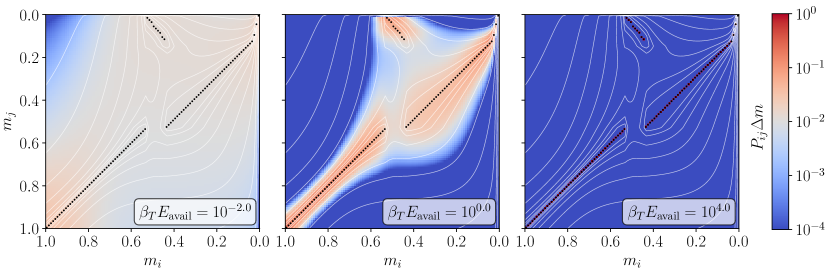
Figure 22: Convergence of $P_{ij}$ [Eq. (52), which is the discrete form of Eq. (47)] to the solution of the LSA problem [black circles; see Section III.1] as $\beta_{T}E_{\mathrm{avail}}\to\infty$ for the case of the unstable-upwards profile (15). Contours of the normal from of the cost matrix $\tilde{\mathcal{E}}_{ij}$ visualized in Fig. 5 are plotted in white.

On physical grounds, we expect that the $\beta_{T}\to\infty$ limit of Eq. (40) [or its equivalent, Eq. (47)], i.e., the limit of zero statistical mechanical temperature, corresponds to the smallest energy permitted by the system, i.e., the result of solving the linear sum assignment (LSA) problem (Section III). We now verify that that the solution to the LSA problem is indeed recoverable from Eq. (47) in the $\beta_{T}\to\infty$ limit.

Because the LSA problem is discrete, it is strictly the $\beta_{T}\to\infty$ limit of Eqs. (42), (43) (44) and (47) only after they are discretized over a small but finite scale $\Delta m$ (we consider reversing the order of the $\Delta m\to 0$ and $\beta_{T}\to\infty$ limits in Section IV.4). We adopt the economical notation ${P_{ij}\equiv P(m_{j},m_{i})}$, $\mathcal{E}_{ij}\equiv\mathcal{E}(m_{j},s_{i},\chi_{i})=\mathcal{E}(m_{j},m_{i})$ and $\psi_{i}\equiv\psi(m_{i})$. Converting integrals to sums, Eqs. (42), (43) (44) and (47) become

$$\Delta m\sum_{i}P_{ij}=1,$$ (48)

$$\Delta m\sum_{j}P_{ij}=1,$$ (49)

$$\Delta m^{2}\sum_{ij}\mathcal{E}_{ij}P_{ij}=E$$ (50)

and

$$P_{ij}=\frac{1}{\Delta m}\frac{\displaystyle e^{\displaystyle-\beta_{T}(\mathcal{E}_{ij}-\psi_{i})}}{\displaystyle\sum_{k}e^{\displaystyle-\beta_{T}(\mathcal{E}_{kj}-\psi_{k})}},$$ (51)

respectively. We define ${\tilde{\mathcal{E}}_{ij}=\mathcal{E}_{ij}-a_{j}-b_{i}}$ and ${\tilde{\psi}_{i}={\psi_{i}-b_{i}}}$, whence

$$P_{ij}=\frac{1}{\Delta m}\frac{\displaystyle e^{\displaystyle-\beta_{T}(\tilde{\mathcal{E}}_{ij}-\tilde{\psi}_{i})}}{\displaystyle\sum_{k}e^{\displaystyle-\beta_{T}(\tilde{\mathcal{E}}_{kj}-\tilde{\psi}_{k})}}.$$ (52)

The advantage to introducing the “tilded” variables in Eq. (52) is that we may always choose the functions $b_{i}$ and $a_{j}$ to be such that $\tilde{\mathcal{E}}_{ij}$ is the normal form of the cost matrix ${\mathcal{E}}_{ij}$ [see Eq. (25)]. As explained in Section III.1, this means that $\tilde{\mathcal{E}}_{ij}\geq 0$ and has at least one zero in each row and column, or, equivalently, there exists at least one bijection $\sigma$ such that $\tilde{\mathcal{E}}_{i\sigma(i)}=0$ for all $i$ [$j=\sigma(i)$ constitutes an optimal assignment for the LSA problem].

In the simplest case, $\tilde{\mathcal{E}}_{ij}$ has exactly one zero in each row and column. We expect this to be the generic case, and, indeed, this is true for all of the profiles examined in Section III.3. These zeros define the unique optimal assignment $j=\sigma(i)$ — taking $\tilde{\psi}_{i}=0$ [the natural choice, as with only one zero in each row and column, the “exclusion principle” is obeyed automatically and the constraint (49) becomes superfluous] then implies that

$$P_{ij}\to\begin{cases}1/\Delta m&\mathrm{if}\,\,\tilde{\mathcal{E}}_{ij}=0,\\ 0&\mathrm{otherwise}.\end{cases}$$ (53)

Thus, in the $\beta_{T}\to\infty$ limit, the system is certain to found in the state given by the optimal assignment $\sigma$ for the LSA problem. Eq. (53) straightforwardly satisfies Eq. (49) — the sum picking out the single value of $j$ for which $P_{ij}\neq 0$ for any given $i$ — which justifies formally our setting ${\tilde{\psi}_{i}=0}$. Substituting Eq. (53) into Eq. (50) yields

$$E=\Delta m\sum_{i}\mathcal{E}_{i\sigma(i)}=E_{\mathrm{min}}.$$ (54)

The convergence of Eq. (52) to the minimum-energy state as $\beta_{T}\to\infty$ is visualized in Fig. 22. The numerical method that we use to compute $P_{ij}$ (here and elsewhere in the paper) is a minor modification of the one described in Appendix B of Ref. [29].

In principle, $\tilde{\mathcal{E}}_{ij}$ may have more than one zero in each row and column: these may either be part of other optimal assignments or not be part of any optimal assignment. We consider these cases in Appendix E, showing that the $\beta_{T}\to\infty$ limit of $P_{ij}$ can always be written as a linear superposition of the permutation matrices that correspond to the optimal assignments of the LSA problem.

IV.4 Large-$\beta_{T}$ limit of continuous Lynden-Bell statistical mechanics

In Section IV.3, we determined that the discretized probability-density function $P_{ij}$ reproduces the solution of the LSA problem (or some weighted combination of its solutions if they are not unique) as $\beta_{T}\to\infty$ at fixed $\Delta m$. This is not, however, the large-$\beta_{T}$ limit of the continuous system (44), (43) and (47): discretizing the integrals is valid only if $\Delta m$ is small compared to the scale of variation of the continuous probability density $P(m,\mu)$, which shrinks to zero as ${\beta_{T}\to\infty}$. Nonetheless, the $\beta_{T}\to\infty$ limit of the continuous Lynden-Bell equations is equal to the $\Delta m\to 0$ limit of the coarse-grained solution of the LSA problem, provided it is unique, as we now show.

Let us consider approaching the continuous limit in the discrete problem by increasing $\beta_{T}$ with $\Delta m$ kept small compared with the width of $P_{ij}$. Intuitively, as the expectation energy $E$ decreases, the weights the permutation matrices in the Birkhoff-von Neumann decomposition of the doubly stochastic matrix $P_{ij}$ [see Eq. (78) of Appendix E] that deviate significantly from the “valleys” of the energy landscape defined by $\tilde{\mathcal{E}}_{ij}$ must decrease, and $P_{ij}$ becomes increasingly localised to the (assumed unique) optimal solution of the LSA problem. In other words, the $\beta_{T}\to\infty$ limits of both the continuous $P$ and the coarse-grained discrete solution $P_{ij}$ of the LSA problem, which we define by

$$\langle P\rangle\equiv\frac{1}{2n}\int^{m+n\Delta m}_{m-n\Delta m}\mathrm{d}m^{\prime}\int^{\mu+n\Delta m}_{\mu-n\Delta m}\mathrm{d}\mu^{\prime}\\ \times\sum_{ij}P_{ij}\delta(\mu-m_{i})\delta(m-m_{j}),$$ (55)

with $n$ a constant satifying $1\ll n\ll N$, each tend to a delta distribution centred on the optimal-solution curve. The most general form such a distribution can take is

$$A(m,\mu)\delta(F(m,\mu))$$ (56)

where $F$ vanishes along the optimal-solution curve and, without loss of generality, can be taken to have ${|\bm{\nabla}F|=1}$ there [$F$ contributes no further degrees of freedom in the expression (56)]. However, as we show in Appendix F, the function $A(m,\mu)$ is uniquely determined by the conditions (48) and (49), which must be satisfied by both $\langle P\rangle$ and $P$. It follows that their large-$\beta_{T}$ limits are the same. A neat practical consequence of this is that one can determine the horizontal composition of 2D minimum-energy ground states from the $\beta_{T}\to\infty$ limit of $P(m,\mu)$.

IV.5 Diffusive stage of relaxation

We now consider the problem of extracting measurable predictions from our Lynden-Bell statistical mechanics. The usual approach to doing so is to argue that, because of the assumed stochastic nature of the underlying microstate, physically measurable quantities are expectation values, i.e.,

$$\langle s\rangle \equiv\int\mathrm{d}s\int\mathrm{d}\chi\,sP(m,s,\chi),$$ (57)

$$\langle\chi\rangle \equiv\int\mathrm{d}s\int\mathrm{d}\chi\,\chi P(m,s,\chi).$$ (58)

It is clear that, being averages, $\langle s\rangle$ and $\langle\chi\rangle$ are not in general obtainable by rearrangement of the the original equilibrium. This is not a contradiction of our assumption of non-diffusive relaxation if we interpret Eqs. (57) and (58) as statistical quantities that agree with measurements on average, but still believe that the true structures of $s$ and $\chi$ are stochastic. In reality, however, we do not expect the final state of the relaxation to be stochastic: once gradients of $s$ and $\chi$ become sufficiently large, their fine-scale structure will be erased by diffusion [we have already seen this happen the simulation visualized in Fig. 2]. It is tempting, therefore, to interpret Eqs. (57) and (58) as providing a model of the smooth, diffused state that develops after diffusion acts on the stochastic final state of the “ideal” relaxation, whose statistics are encoded by $P(m,s,\chi)$. We plot $\langle s\rangle$ and $\langle\chi\rangle$ against $z$ [taking the density to be ${\rho(m,\langle s\rangle,\langle\chi\rangle)}$] with a gold dashed line in Fig. 23 for each of the profiles considered in Section III.3.

There is, however, a problem with this interpretation: the energy associated with the coarse-grained state given by $\langle s\rangle$ and $\langle\chi\rangle$ is not equal to the energy (37) of the fine-grained state, i.e.,

$$\int\mathrm{d}m\,\mathcal{E}(m,\langle s\rangle,\langle\chi\rangle)\neq E,$$ (59)

because $\mathcal{E}(m,s,\chi)$ is nonlinear in $s$ and $\chi$. In the terminology of Chavanis [28], energy is a “fragile integral” — its value is different depending on whether it is computed using the coarse- or fine-grained distributions of $s$ and $\chi$. Indeed, the amount of energy that is “missing” is typically much greater than the available energy of the metastable equilibrium — around ten times greater in the case of the unstable-upwards profile defined by Eq. (15). Evidently, this is a problem: diffusion should conserve total energy. The natural fix is to compute the entropy after diffusion, which we denote $\bar{s}$, not via Eq. (57) (which is manifestly a poor model — diffusion does not conserve entropy, particularly in the presence of resistive heating) but by imposing the conservation of $\mathcal{E}$ at $m$, i.e., via

$$\mathcal{E}(m,\bar{s},\bar{\chi})=\int\mathrm{d}s\int\mathrm{d}\chi\,\mathcal{E}(m,s,\chi)P(m,s,\chi),$$ (60)

with the diffused magnetic flux $\bar{\chi}$ satisfying

$$\bar{\chi}=\langle\chi\rangle$$ (61)

(diffusion does conserve magnetic flux). Eq. (60) models energy-conserving diffusion that acts locally in space, smoothing the arbitrarily small-scale stochastic structure associated with $P(m,s,\chi)$. We plot $\bar{s}$ and $\bar{\chi}$ against $z$ [with density ${\rho(m,\bar{s},\bar{\chi})}$] with a solid cyan line in Fig. 23.

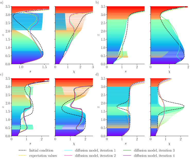
Figure 23: The predictions of the Lynden-Bell statistical mechanics [Section IV.1] for each of the profiles described in Section II.3: Panels (a) correspond to Eq. (15), Panels (b) to Eq. (16), Panels (c) to Eq. (17) and Panels (d) to Eq. (18). In each case, the black dashed line corresponds to the initial profile, the gold dashed line to the expectation values of $P(m,s,\chi)$ [Eqs. (57) and (58)] and the cyan solid line to the prediction of Eqs. (60) and (61). Other colored lines correspond to iterations of the statistical mechanical predictions based on the profiles calculated from Eqs. (57) and (58) — see the main text for details.

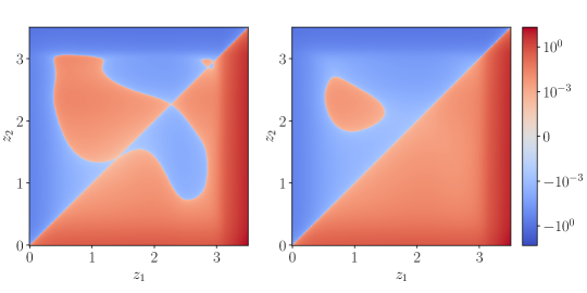
Figure 24: The force [Eq. (3)] per unit mass of a small fluid parcel moved in pressure balance and without diffusion from height $z_{1}$ to $z_{2}$ for: left panel, the state that corresponds to the cyan lines in Fig. 23(a); and, right panel, the analogue of this profile for $E=E_{0}+0.3E_{\mathrm{avail}}$. The left panel exhibits linear instability, the right panel nonlinear instability (metastability).

A question of obvious concern is whether the state obtained from Eqs. (60) and (61) is stable, linearly or nonlinearly — i.e., whether it is the state of minimum energy subject to ideal rearrangements of the new entropy and flux profiles. Remarkably, the answer is often no: diffusion of the “statistically most likely” state to be reached under ideal relaxation tends to produce states that are unstable to further (ideal) dynamics. This is is a consequence of the fact that diffusion produces density changes, and is reminiscent of the phenomenon of “buoyancy reversal” in terrestrial atmospheres, whereby the nonlinear dependence of density on advected invariant quantities (water content, in that context) means that a buoyant parcel of fluid that rises and mixes with denser ambient fluid can become denser than the ambient fluid, and sink as a result. Either linearly unstable or nonlinearly unstable (metastable) states are possible outcomes of Eqs. (60) and (61). This is illustrated by Fig. 24: Panel (a) plots the force (3) per unit mass on a small parcel of fluid displaced from height $z_{1}$ to $z_{2}$ [as in the lower panels of Fig. 3] for the state that results from Eqs. (60) and (61), in the case of the metastable-upwards equilibrium (15), with $E$ in Eq. (37) chosen to be equal to the total potential energy $E_{0}$. We find that the predicted state is linearly unstable between $z\simeq 1.4$ and $z\simeq 2.3$, and also close to $z=3$. Panel (b) shows the same quantity, but for a slightly larger energy of $E=E_{0}+0.3E_{\mathrm{avail}}$ in Eq. (37) (this is the initial energy of the numerical simulation to be presented in Figs. 25 and 26 in Section V.1). In this case, the new profile is linearly stable, but is unstable nonlinearly (metastable), and turns out to have a state with lower energy (as can be confirmed by solving its LSA problem). Likewise, the profiles obtained by applying Eqs. (60) and (61) in the cases of “bi-directional” [Eq. (17)] and “overturning” [Eq. (18)] profiles are not minimum-energy states, but it turns out that Eqs. (60) and (61) do yield a minimum-energy state in the case of the unstable-downwards profile (16).

One could argue (reasonably) that, in cases where it is unstable, the equilibrium predicted by Eqs. (60) and (61) would never be reached. Evidently, a linearly unstable state cannot be the end point of the relaxation. Less obviously, we might also suppose that, given an initial perturbation of sufficient strength, the chaotic flows that develop during relaxation will be enough to displace the relaxing profile from any metastable state that it might develop. However, if diffusion is always much slower than ideal dynamics (as we have been assuming), the “ideal” stochastic relaxed state should develop, diffuse, and, if that state is unstable, relax again under new ideal dynamics, i.e., under the assumptions outlined in Section IV.1. This process would repeat until a state was established that had no energetically profitable rearrangements, i.e., a minimum-energy state. Such a state could be predicted theoretically by applying Lynden-Bell statistical mechanics in an iterative manner: first, one would compute the Lynden-Bell prediction for $P(m,s,\chi)$, then apply the local model of diffusion summarized by Eqs. (58) and (60) to produce new profiles of $s$ and $\chi$. These new profiles could then be used as starting profiles for a new Lynden-Bell calculation (with the same total energy) and this process repeated until convergence, which would occur when the diffused state was stable to ideal rearrangement (both linearly and nonlinearly). The results of this procedure are shown in Fig. 23, with the $\bar{s}$ and $\bar{\chi}$ at the second, third and fourth iterations plotted in pink, green and purple, respectively. The procedure terminates after a second iteration in the unstable-upwards [Eq. (15)] and “overturning” [Eq. (17)] cases [see panels (a) and (d)], and after a fourth iteration in the unstable-“bi-directional” case. [NB: in the “overturning” case, we find at the fourth iteration that the state is sufficiently close to the ground state to become sensitive to the discretization that we employ to compute the integrals in Eqs. (58) and (60) — see the jagged structure of the purple line in panel (c) of Fig. 23. At the fifth iteration, $\beta_{T}$ becomes so large as to prevent accurate computation of the relevant integrals, so we terminate the process at the fourth iteration.]

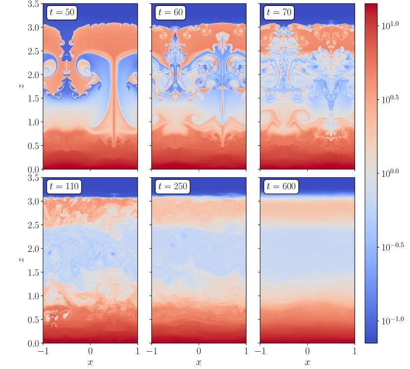
Figure 25: Numerical simulation of the relaxation of the equilibrium defined by Eq. (15) at $\mathrm{Re}\sim 10^{5}$. The quantity plotted is the ratio $s/\chi$. The initial velocity field is given by Eq. (34) with $u_{0}=0.1$, $z_{0}=1.0$ and $\Delta z=0.5$, which corresponds to $E_{\mathrm{kin},0}\simeq 0.3E_{\mathrm{avail}}$.

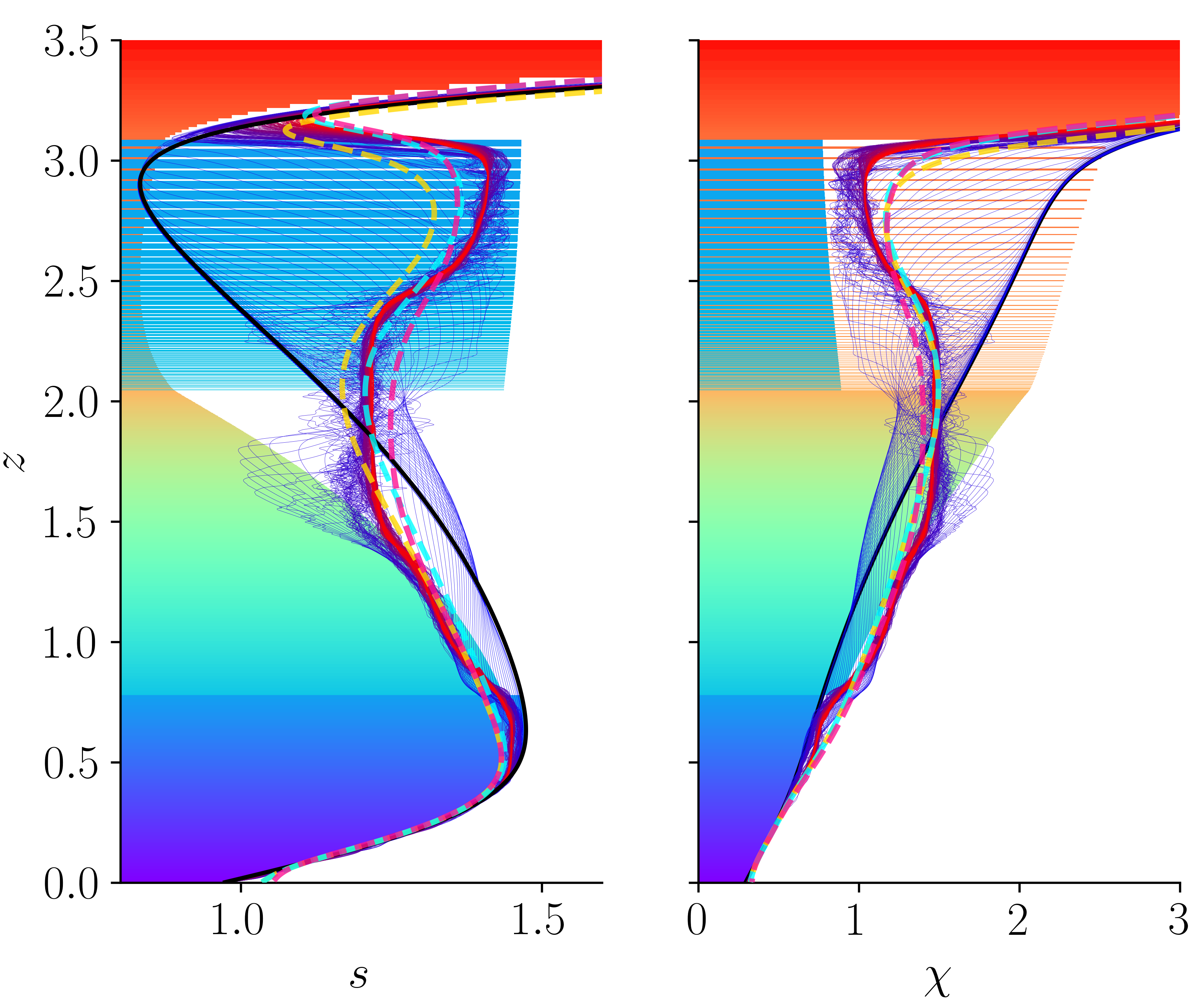
Figure 26: Horizontally averaged profiles of $s$ and $\chi$ plotted at intervals of $1$ code time unit, between $t=0$ (blue) to $t=600$ (red), for the simulation visualized in Fig. 25. Also plotted are the profiles obtained by taking expectation values of $P(m,s,\chi)$ (gold dashed line; we argue in the main text that this prediction is to be rejected on theoretical grounds), from Eqs. (60) and Eq. (61) (cyan dashed line), and after iterating the statistical mechanical prediction from the profile based on the cyan dashed line (pink dashed line). For reference, we also plot the minimum-energy state — this is as shown in Fig. 4.

The discussion above may well strain the credulity of the reader to whom the idea of the sequential relaxation that we have described, entailing complete ideal relaxation in multiple stages, seems dubious. Such a reader may be reassured by the fact that the difference in the profiles of $\bar{s}$ and $\bar{\chi}$ between the first and last stages of the procedure turn out to be very slight — thus, under the circumstances that the secondary relaxation are incomplete, or that diffusion occurs concurrently with them, we can expect that the final state reached might not be very different. We shall see in Section V that accounting for these diffusive rearrangements is, in practice, something of a precision overkill — greater discrepancies between numerical experiment and the theoretical prediction arise which appear to be a result of the tendency of relaxing profiles to become “stuck” in other metastable states. Nonetheless, it is interesting to note that, on a qualitative level, the way that stability is ultimately achieved in the iterative procedure is via the formation of plateaus. In the case of the unstable-upwards profile, for example, we see from Fig. (23)(a) that, between the first and second iterations, material at $z\lesssim 1.75$ moves upwards to settle in the range $1.75\lesssim z\lesssim 2.75$, producing a flatter region between $2.5\lesssim z\lesssim 3.0$ and in the vicinity of $z\simeq 2$. Similar plateaus are observed in panels (c) and (d), with the particular case of panel (c) resembling a staircase profile. The intriguing possibility of modelling the formation of staircases (which are observed in myriad diffusing systems in geo- and astro-physical contexts) statistical mechanically is a topic to which we shall return in future work.

For completeness, we note that the relevant analogue of Eqs. (57) and (58) for the collisionless-relaxation problem, i.e.,

$${\langle\eta\rangle=\int\mathrm{d}\eta P(\bm{v},\eta)}$$ (62)

[see below Eq. (40) for relevant definitions], does constitute a plausible prediction for the particle-distribution function in the presence of small collision frequency (collisions act as diffusion in velocity space, smoothing the stochastic variation in the local value of $\eta$ to its mean). This is because collisions preserve the contribution of each patch of phase space to the total energy, momentum and number of particles, as these quantities are each linear in $\eta$. In the language of Chavanis [28], total energy, momentum and number of particles are “robust integrals”, being the same for both the coarse- and fine-grained distributions of $\eta$ [although, see the discussion in Section VI.2].

V Numerical simulations at large Reynolds number

In this section, we present a comparison of the theoretical predictions obtained in Section IV.5 with the results of numerical simulations conducted at $\mathrm{Re}\gg 1$. The numerical setup is the same as in Section III.4, but with the kinematic viscosity $\nu$ smaller by a factor of $400$, such that the Reynolds number based on the initial velocity field is $u_{0}L_{x}/\nu\sim 10^{5}$.

V.1 Upwards metastability, Eq. (15)

We first consider the case of the unstable-upwards profile defined by Eq. (15). Fig. 25 visualizes the distribution of $s/\chi$ (the advected scalar that controls the fluid compressibility — see Section II) during the relaxation that follows perturbation by a velocity field given by Eq. (34) with $u_{0}=0.1$ and $z_{0}=1.0$ (this corresponds to an initial kinetic energy $E_{\mathrm{kin},0}\simeq 0.3E_{\mathrm{avail}}$). We observe that a substantial plume of material rises until reaching the stable region at the top of the simulation domain, where it overturns, develops Rayleigh-Taylor instabilities, and, under advection by the increasingly chaotic flow, develops small-scale structure (upper three panels). These structures diffuse, ultimately leading a smooth, one-dimensional but non-homogeneous state (lower three panels).

Fig. 26 compares the horizontally averaged instantaneous profiles of $s$ and $\chi$ developed over the course of the simulations with both $\langle s\rangle$ and $\langle\chi\rangle$ [Eqs. (57) and (58)] and $\bar{s}$ and $\bar{\chi}$ [Eqs. (60) and (61)] at the first and second iterations of the procedure described in Section IV.5. The quantities are computed from $P(m,s,\chi)$ calculated with $E=E_{0}+E_{\mathrm{kin},0}$. [NB. The Mach number of the simulation, $\mathrm{Ma}\equiv u_{0}/\sqrt{v_{A}^{2}+c_{s}^{2}}\sim 0.1$ is small, so that the compressible part of the initial velocity field rapidly propagates away as compressive waves. The energy associated with these waves (i.e., the initial energy of the non-solenoidal part of $\bm{u}$) is, we assume, irrelevant to the otherwise quasi-incompressible dynamics, so we exclude it from the energy we use for $E$ in Eq. (37).]

We make the following observations. First, we note that the late-time profile of $s$ is almost everywhere larger than $\langle s\rangle$ [Eq. (57); gold dashed line in Fig. 26]. This validates the reasoning we used to reject Eq. (57) as a predictor of the final state — evidently, non-ideal effects like viscous and resistive heating cause the entropy of the fluid to grow.

Secondly, we observe that $\bar{s}$ and $\bar{\chi}$ computed at the first iteration of the procedure described in Section IV.5 [Eqs. (60) and (61); cyan dashed line in Fig. 26], constitute a very reasonable prediction of the relaxed state. The chief discrepancies are in the range $2.5\lesssim z\lesssim 3.0$, where $\bar{s}$ and $\bar{\chi}$ are, respectively, somewhat smaller and larger than in the late-time profiles developed by the simulation. We interpret this as a consequence of the system not “exploring” the full surface of constant energy in configuration space, owing to the fluid that rises from the bottom of the equilibrium becoming trapped in a metastable state at the top. In support of this interpretation, we note that, in the range $0.9\lesssim z\lesssim 1.5$, the cyan lines somewhat over- and under-predict the simulation result, respectively, indicating that “too much” material rose in the initial plume (and got stuck). A second discrepancy between the cyan line and the simulation result is that the latter exhibits a clear plateau in the range $1.5\lesssim z\lesssim 2.3$, which does not appear in the theoretical prediction. As noted in Section IV.5, plateaus may form when the ideal relaxed state becomes unstable after diffusion. Indeed, the state represented by the cyan line is nonlinearly unstable [see Fig. 3(b) for its force diagram] and develops a plateau at the second application of the statistical procedure [dashed pink line in Fig. 26]. This plateau is predicted to develop over roughly the same range of $z$ as the one that forms in the simulation, although the predicted plateau has slightly larger $s$ (smaller $\chi$). This can be interpreted as a consequence of the fact that the large-$s$ fluid that would have risen upwards under the secondary relaxation to form the plateau was, in the simulation, already displaced to the top of the atmosphere. As a consequence, the plateau forms with somewhat smaller $s$ than it would otherwise have had.

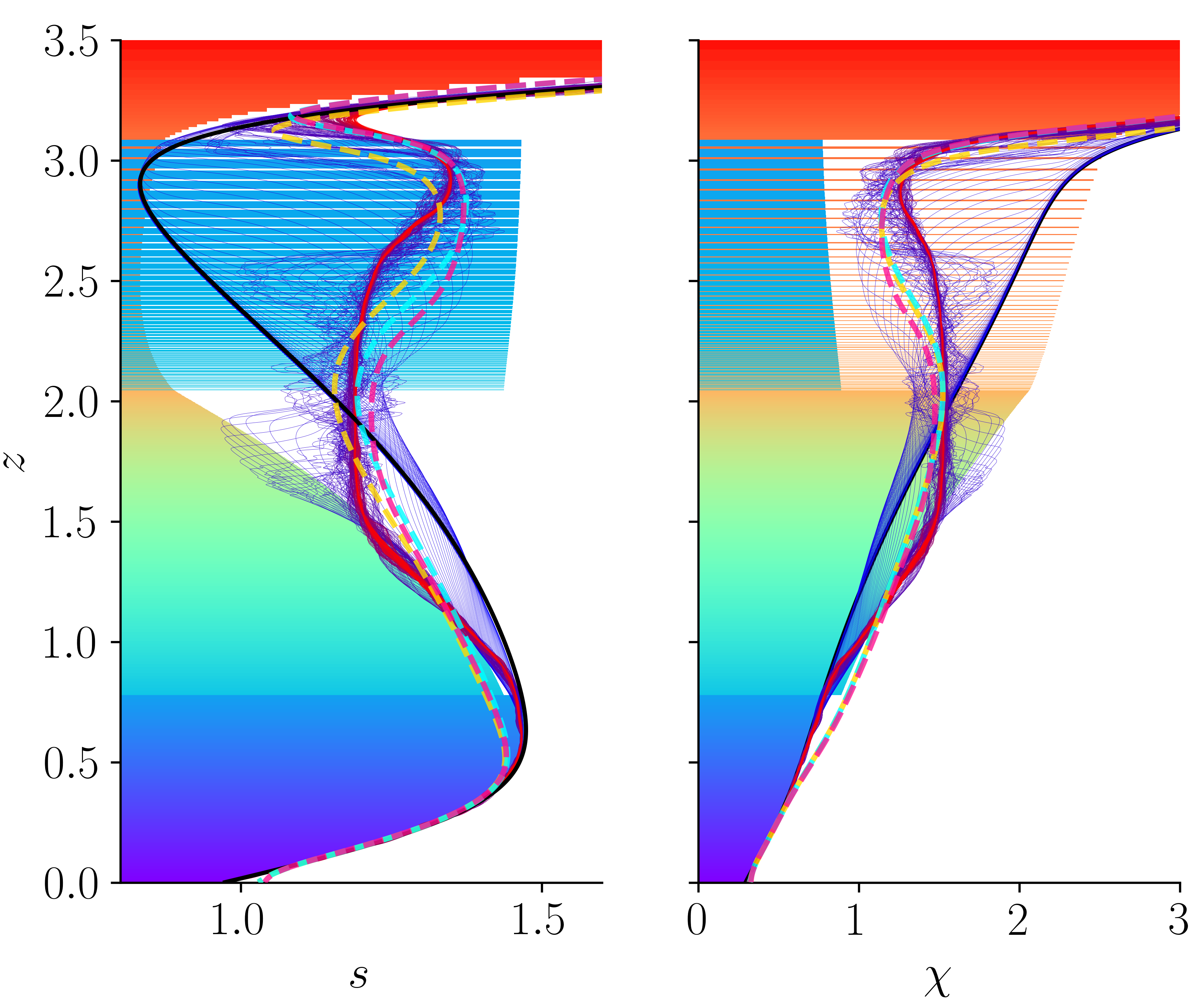
Figure 27: As in Fig. 26, but for a simulation initialised with $u_{0}=0.05$ in Eq. (34) ($E_{\mathrm{kin},0}\simeq 0.1E_{\mathrm{avail}}$).

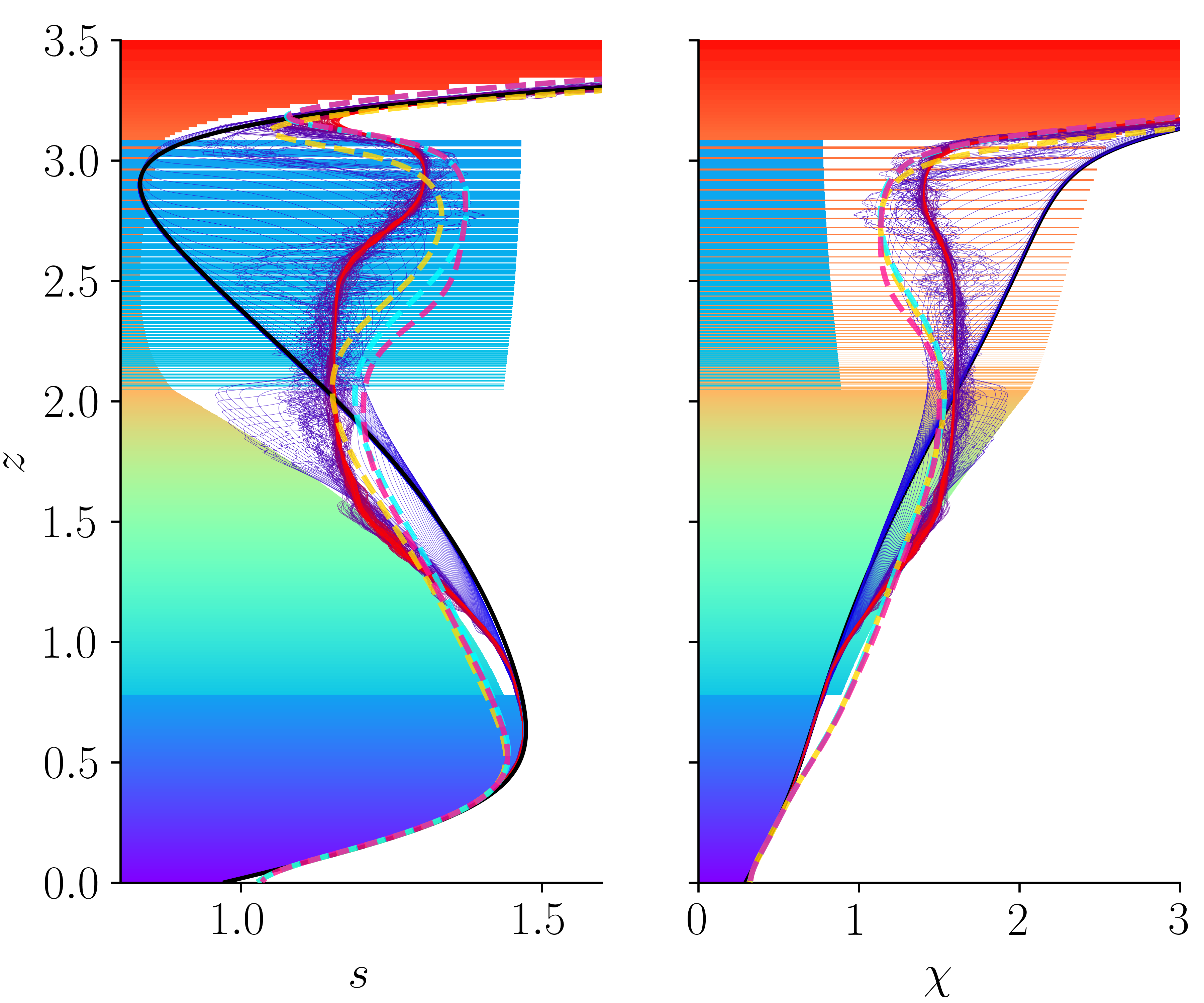
Figure 28: As in Fig. 26, but for a simulation initialised with $u_{0}=0.025$ in Eq. (34) ($E_{\mathrm{kin},0}\simeq 0.02E_{\mathrm{avail}}$).

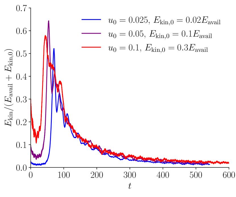
Figure 29: Evolution of the kinetic energy as a fraction of the total available energy, which is the kinetic energy plus the available potential energy of the initial state, for the simulations visualized in Figs. 26, 27 and 28.

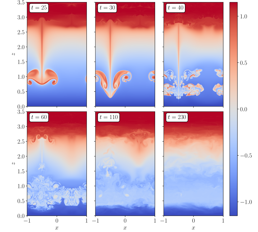
Figure 30: Numerical simulation of the relaxation of the equilibrium defined by Eq. (16) at $\mathrm{Re}\sim 10^{5}$. The quantity plotted is the ratio $s/\chi$. The initial velocity field is given by Eq. (34) with $u_{0}=0.1$, $z_{0}=2.25$ and $\Delta z=0.5$; this corresponds to an initial kinetic energy $\simeq 0.2$ times the available potential energy.

Figure 31: Horizontally averaged profiles of $s$ and $\chi$ plotted at intervals of $1$ code time unit, between $t=0$ (blue) to $t=600$ (red), for the simulation visualized in Fig. 30. Also plotted are the profiles obtained by taking expectation values of $P(m,s,\chi)$ (gold dashed line; we argue in the main text that this prediction is to be rejected on theoretical grounds) and from Eqs. (60) and Eq. (61) (cyan dashed line).

Figure 32: As in Fig. 31, but for a simulation initialised with $u_{0}=0.1$ in Eq. (34), which corresponds to ${E_{\mathrm{kin},0}\simeq 0.1E_{\mathrm{avail}}}$.

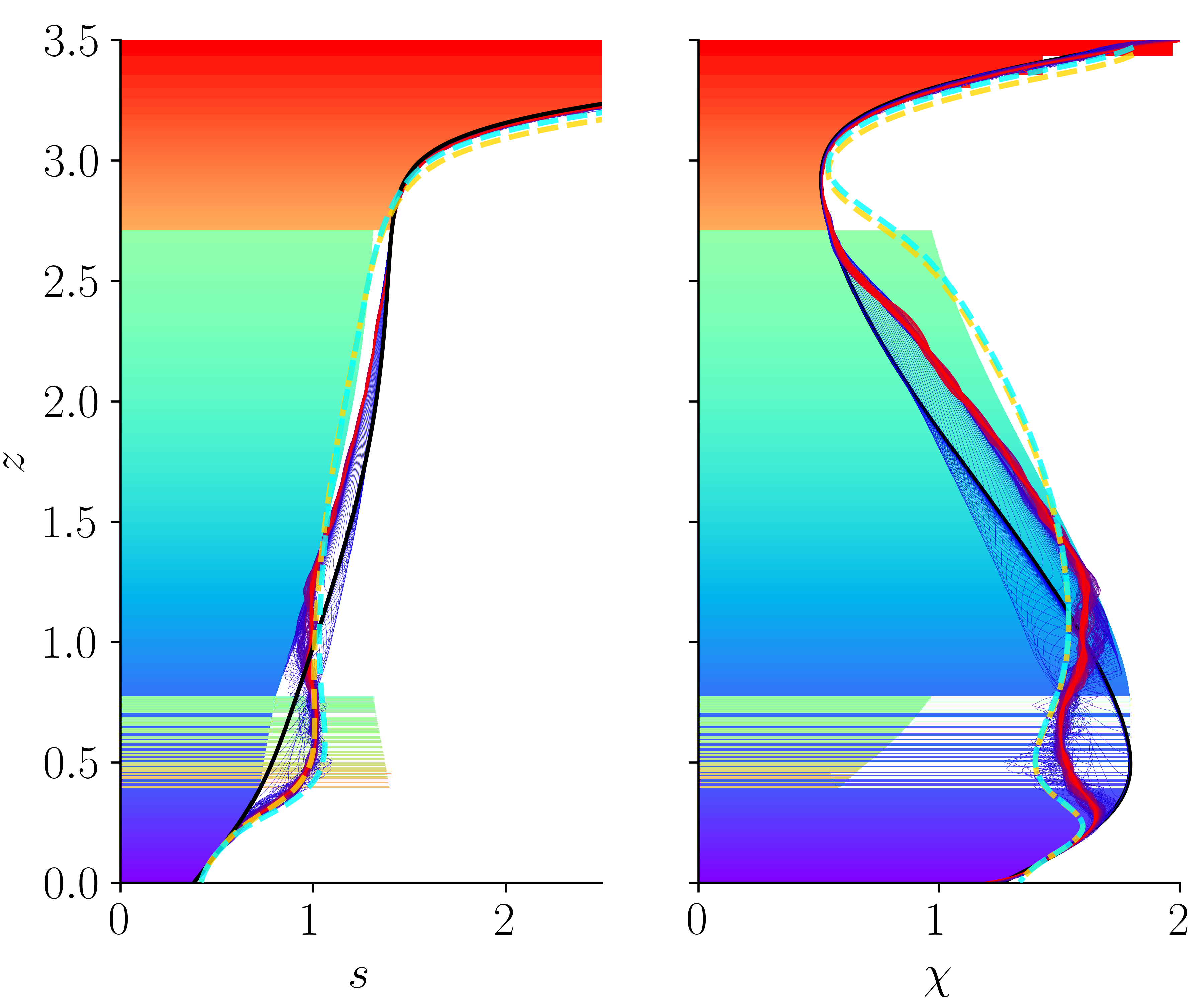
Figure 33: As in Fig. 31, but for a simulation initialised with $u_{0}=0.05$ in Eq. (34), which corresponds to ${E_{\mathrm{kin},0}\simeq 0.03E_{\mathrm{avail}}}$.

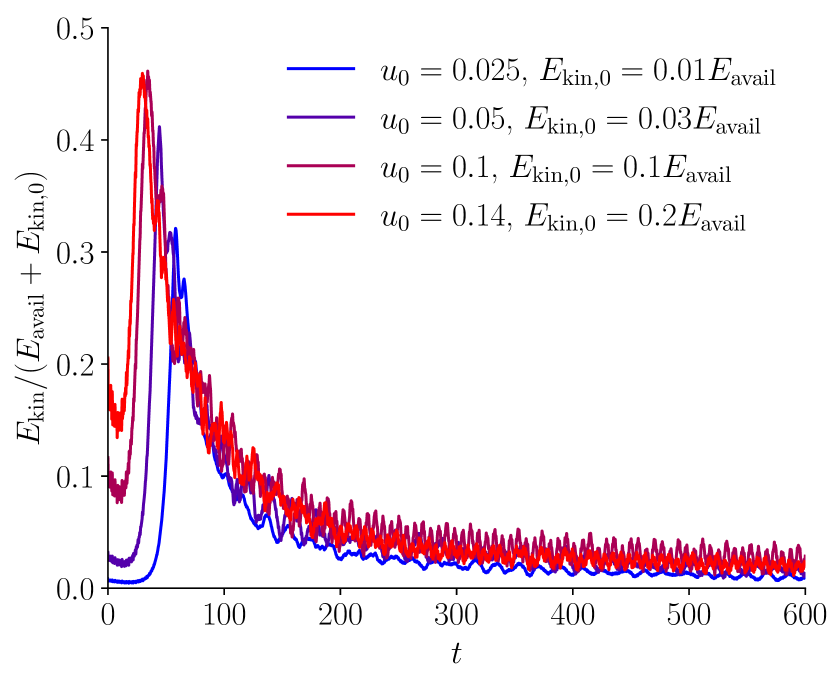
Figure 34: Evolution of the kinetic energy as a fraction of the total available energy, which is the kinetic energy plus the available potential energy of the initial state, for the simulations visualized in Figs. 31, 32 and 33, as well as for one with $u_{0}=0.025$ in Eq. (34).

Figs. 27 and 28 are analogous to Fig. 26 but for simulations with ${u_{0}=0.05}$ ($E_{\mathrm{kin},0}\simeq 0.1E_{\mathrm{avail}}$) and ${u_{0}=0.025}$ ($E_{\mathrm{kin},0}\simeq 0.02E_{\mathrm{avail}}$), respectively. In these cases, the agreement between simulation and theory is less good, but remains fair. As explained in Section III.4.1, a sufficiently large initial perturbation is required to overcome the potential barrier that forms during relaxation (even though the initial state is at marginal linear stability) and hinders further relaxation. Fig. 29, shows that, at peak, between $50\%$ and $60\%$ of the available kinetic plus potential energy is in the form of kinetic energy for all three simulations, showing that the liberation of available potential energy during relaxation is fairly efficient.

V.2 Downwards metastability, Eq. (16)

We report in this section the results of analogous simulations to those presented in Section V.2, but for the unstable-downwards profile defined by Eq. 16.

Fig. 30 visualizes the evolution in $x$-$z$ space for ${u_{0}=0.14}$ ($E_{\mathrm{kin},0}\simeq 0.2E_{\mathrm{avail}}$), following the tracer $s/\chi$. Analogously to the evolution displayed in Fig. 25, we observe that a descending plume reaches the stable buffer region at the bottom of the simulation domain, develops small-scale structure via Rayleigh-Taylor instability and advection by chaotic motions, and ultimately diffuses. The evolution of the horizontally averaged profiles is displayed in Figs. 31, 32 and 33 for the cases of $u_{0}=0.14$ ($E_{\mathrm{kin},0}\simeq 0.2E_{\mathrm{avail}}$), $u_{0}=0.1$ ($E_{\mathrm{kin},0}\simeq 0.1E_{\mathrm{avail}}$), and $u_{0}=0.05$ ($E_{\mathrm{kin},0}\simeq 0.03E_{\mathrm{avail}}$), respectively. Again, we observe reasonable agreement between the statistical mechanical prediction and the late-time limit of the simulations, although the predictions do somewhat under-predict $s$ and over-predict $\chi$ for $z\gtrsim 1.5$. Again, the reason appears to be partial relaxation: the degree of inaccuracy is greater in the simulations with smaller initial velocity fields. We also note that the theory fails to predict a plateau in the vicinity of $z\simeq 0.5$ (no further ideal relaxation is predicted from the diffused state that corresponds to the cyan line) — such a plateau is present, to some degree, in all three simulations. Nonetheless, the theoretical predictions agree well in this region with all three simulation profiles, the flatness notwithstanding. Finally, in Fig. 34, we show the evolution of the kinetic energy as a fraction of the total available energy. Again, we see that the relaxation is fairly efficient at liberating available potential energy, and that large initial perturbations are not required to do so: over a factor $\simeq 30$ difference in the initial kinetic energy, the peak ratio of kinetic energy to available energy varies only between around $30\%$ and $45\%$.

VI Conclusion

VI.1 Summary

In this work, we have demonstrated that magnetic-field-line bending is not an essential ingredient for the metastability of a stratified MHD equilibrium: metastable equilibria exist even in the simple case of 2D MHD with out-of-plane magnetic field, i.e., where the sole role of the magnetic field is to provide a source of pressure. Metastability is, in this case, a consequence of the fact that fluid with large plasma $\beta$ is more compressible than fluid with small $\beta$, meaning that, when displaced by a large distance and thus exposed to a large change in pressure, the density of large-$\beta$ fluid can be less than that of the ambient fluid at the new location, even if this would not be the case for sufficiently local (i.e., linear) displacements.

The existence of metastability in 2D, rather than only in 3D, is interesting chiefly because the ideal (i.e., dissipationless) relaxation of a 2D metastable state constitutes rearrangement of parcels of fluid subject to the parcel-wise conservation of specific entropy and magnetic flux. This enables the use of combinatorial and statistical techniques that are apparently unavailable for the 3D problem (although see Section VI.2). We have determined the minimum-energy state consistent with 2D rearrangements by solving a linear sum assignment (LSA) problem in four different illustrative cases. We find that the available potential energy is generally small, a result that can be traced back to the fact that fluid parcels exclude each other, so that the mass of fluid that can experience a large change in pressure is limited. An interesting finding is that the minimum-energy states are two dimensional, despite the initial profiles being one dimensional (all quantities depend on height only). We show that the relaxed state that develops in numerical simulations at small Reynolds number approximates the 2D minimum-energy state, as the potential energy liberated during relaxation is dissipated by viscosity (changing the entropy of the fluid only slightly, owing to the small energy scales involved).

The two-dimensionality of the minimum-energy states may be interpreted as a consequence of the fact that the one-dimensional states that can be reached by rearranging slices of fluid of finite width to reduce the total potential energy are, in general, Rayleigh-Taylor unstable. Provided that it is not suppressed by viscosity, the instability (and the potential energy liberated during relaxation) drives a turbulent flow that generates small scale structure, enabling diffusion to act and violate the fluid-element-wise conservation of entropy magnetic flux. We have proposed that such cases can be modelled theoretically by invoking (non-rigorously, but, apparently, usefully) a separation of timescales between the one on which the flow is mixed (i.e., the ideal dynamical timescale) and the one on which the advected invariants diffuse. We suggest that the end state of the former relaxation is the equilibrium state that maximizes the Boltzmann mixing entropy subject to fixed energy — this is analogous to the Lynden-Bell theory of “violent relaxation” of self-gravitating systems and collisonless plasmas, and to the Robert-Sommeria-Miller (RSM) theory of 2D vortex turbulence. The generalization of these theories to more than one conserved quantity (thermal entropy and magnetic flux) turns out to be uncomplicated — the theory can be recast as a maximization of the mixing entropy associated with rearrangements of 1D slices.

We take the latter, diffusive part of the relaxation to be a homogenization of the stochastic small-scale structure present in a statistical mechanical microstate. It is tempting to argue that this homogenization is to the mean of the statistical mechanical probability distribution function, i.e., to expectation values. However, an interesting complication that arises in our theory (but is absent from the contexts mentioned above) is that the profiles of thermal entropy and magnetic flux that one would obtain by taking expectation values of the statistical mechanical probability distribution do not have the same associated total energy as the initial state: total energy is not a “robust integral”. This is a consequence of the nonlinear dependence of energy (enthalpy) density on entropy and magnetic flux. We argue that the correct way to obtain predictions from the probability distribution is to enforce local conservation of enthalpy and magnetic flux, these being quantities that, unlike entropy, are preserved by diffusion.

A related consequence of the nonlinearity of the energy functional is that the states that one derives in the manner described above are not necessarily (or, indeed, usually) stable to ideal dynamics. We propose that a natural scheme for dealing with this, which is consistent with the philosophy of timescale separation between ideal and non-ideal effects, is to iterate the procedure described above for the new profiles — i.e., to seek the mixing-entropy-maximizing ideal rearrangement and then allow diffusion to act upon it — and to continue iterating until a stable profile is reached. Reassuringly (given the heavy reliance that the justification of this scheme has on a dubious separation of timescales), the difference between the profiles predicted at the first and final iterations is not typically very large. Perhaps the most interesting result of this process is that the qualitative result of the subsequent iterations is to produce plateaus in the profiles of $s$ and $\chi$ — see Section VI.2 for further discussion.

We compare the results of 2D numerical simulations of the relaxation of equilibria at marginal linear stability at large Reynolds number (and Prandtl numbers of order unity) with the theoretical predictions described above. Provided that the equilibrium is perturbed sufficiently strongly to generate through mixing, we observe remarkably good agreement between the late-time state of the numerical simulations and the predictions of our statistical mechanical treatment (which, we emphasize, is a theory with no free parameters). We also observe in the simulations the formation of well-mixed plateaus whose properties are consistent with the idea that they are formed by the secondary instability that arises after diffusion. For weak initial perturbations, the agreement between the late-time states of the numerical simulations and our theory is less good. We interpret this as a consequence of the metastability phenomenon itself — when the relaxing system becomes “stuck” in a metastable state, it cannot explore the full constant-energy surface in its configuration space.

VI.2 Discussion

Our study suggests a number of questions for future investigation. One such question concerns the role of metastability in a driven, rather than relaxing, context. The present study has been motivated in part by the fact that, unlike equilibria that are very unstable linearly, equilibria that are strongly metastable (in the sense of having a large amount of available energy) are realizable in real physical systems, by an evolution of the potential-energy landscape that preserves the local minimum (metastable state) within which the system resides. It would be illuminating to understand whether, and under what conditions, the development of metastable state actually occurs in a dynamically evolving system, such as one driven towards convective instability by external heating (and/or cooling). If metastable states do develop, do they relax periodically via sporadic eruptions? How frequent are those eruptions? And are the corresponding relaxations “complete”, in the sense of taking the system far from the linear-stability limit, or does the state of the system always remain close to this limit? Such questions are particularly pertinent in light of the observation that edge-localized modes in tokamaks — which are believed to be manifestations of metastable dynamics in driven systems (see Introduction and Refs. [6, 7, 8, 9, 10]) — are observed to leave the plasma much below the threshold for linear instability post-eruption (see, e.g., [30, 31]).

An obvious question is whether the methods employed within this work can be adapted to fully 3D dynamics. The key challenge there is that, in 3D, $B/\rho$ is not an ideal invariant: the magnetic flux through any material surface is conserved, but the density of the fluid in that surface can change due to motions perpendicular to the surface as well as parallel to it. Thus, relaxation in 3D is not simply a rearrangement of fluid parcels with associated invariants. Non-ideal processes too are significantly more complex in the 3D problem than the simple diffusion of scalar quantities — with magnetic field now a vector, magnetic topology imposes constraints (some, but not all, of which can be broken by magnetic reconnection in the subsequent relaxation [32, 33, 34, 35, 36]). Nonetheless, we remark that the LSA problem could still be employed to calculate a rigorous lower bound on the available energy of an equilibrium with initially straight magnetic field: the smallest potential energy that the field can have under interchanges of field lines evidently constitutes such a bound. Furthermore, it seems plausible that the final state of 3D relaxation would, in fact, be 2D — bent field lines would tend to reconnect and straighten out under magnetic tension. Speculatively, if the development of such a final state were to constitute an effective series of interchanges, the statistical methods developed in this paper might well be applied usefully.

Another intriguing question for future work is whether combinatorial and statistical models of relaxation analogous to those that we have employed here are applicable to the formation of staircases in systems that exhibit double-diffusive convection (e.g., to the famous “thermohaline staircases”, but also to similar staircases in myriad geo- and astro-physical contexts). The existence of staircases in the ocean is well documented and they are observed to be extremely stable — measurements of steps in the salt-fingering staircases have revealed structure that persists over $\sim 100\mathrm{km}$ and for a timescale of years (see Ref. [37] for a review). Metastability to diffusive modes (necessarily diffusive ones — the “ideal” sort of metastability that we have considered in this work does not exist within the Boussinesq approximation in which staircase formation is well known to occur) has been mooted as a possible explanation for staircases (again, see Ref. [37]). Although diffusion is not naturally incorporated into the LSA problem of finding minimum-energy states, one could imagine constructing a scheme for incorporating different rates of diffusion into the iterative model described in Section IV.5. Whether such a scheme would reproduce staircases, or offer qualitative insights into the mechanisms by which they form, remains to be seen. Some cautious optimism can be derived from results like Fig. 23(c), which constitutes a theoretical prediction of a staircase-like structure (although not as a result of double-diffusive instability).

Finally, let us ask whether we have learned any lessons that may be pertinent to “violent relaxation” in other contexts. A simple but useful one is the confirmation that the statistical mechanical theory can work well in predicting relaxed states, provided the system is perturbed sufficiently strongly for it to become well mixed. A second result is that the theory appears to work well in systems that possess more than one invariant. Ref. [29] have speculated about the possibility of predicting the relaxation of a collisionless magnetized plasma by enforcing the conservation of two invariants: the phase-space density $\eta$ and the magnetic moment ${\mu_{b}=mv_{\perp}^{2}/2B}$ (here, $m$ is the mass of a particle, and $v_{\perp}$ is the magnitude of the velocity of the particle in the direction perpendicular to the magnetic field $B$). It is interesting to note that, under such a scheme, the energy $\mathcal{E}$ associated with a volume element of phase space is a nonlinear function of conserved quantities, viz., $\mathcal{E}=\eta(mv_{\parallel}^{2}/2+\mu_{b}B)$. It follows that such a theory would need to address questions similar to the ones we considered in Section IV.5, about how one extracts predictions from the Lynden-Bell probability distribution — the distribution function corresponding to its expectation value will, in general, not have the correct energy. We suggest that the fix might be, as in this work, to acknowledge that diffusion (in this case, particle collisions) does not conserve $\eta$ and $\mu_{b}$, but, rather, $\eta$ and $\mathcal{E}$, and, therefore, to evaluate the distribution function according to a scheme analogous to Eqs. (60) and (61). Whether or not the resulting distribution functions are unstable (as for the profiles that develop due to diffusion in our study), and, if so, the prediction of their further evolution, would, we suggest, be an interesting topic for future exploration.

Appendix A Details of the numerical simulations

The numerical simulations presented in this work were conducted with the finite-difference MHD code Pencil [38]. The code uses sixth-order finite differences and a third-order-accurate time-stepping scheme. In all simulations, we use reflecting boundary conditions (i.e., anti-symmetry of the velocity field in the direction normal to the boundary and symmetry in the other direction) at the boundaries in $z$, while enforcing anti-symmetry relative to the value on the boundary for $B$, $p$ and $\rho$. For the simulations reported in Section I, we simulate directly only the region with $0\leq x\leq 1$ and $0\leq z\leq 3.5$, with reflecting boundary conditions in the $x$ direction (and symmetric boundary conditions for $B$, $p$ and $\rho$) — we construct the visualizations in Figs. 1 and 2 by reflecting the simulation domain in the line $x=0$. For all other simulations, we employ periodic boundary conditions in the $x$ direction (and simulate the full range $-1\leq x\leq 1$). The resolutions of the simulations are $1166\times 4080$ for those reported in Section I, $1166\times 2040$ for those reported in Section III.4, and $2332\times 4080$ for those reported in Section V.

In all simulations, we choose the adiabatic index ${\gamma=5/3}$, magnetic diffusivity ${\eta=4\times 10^{-6}}$ and thermal diffusivity $K=6\times 10^{-6}$. This means that ${\eta/K=2/3=\gamma-1}$, which is the critical ratio for stability to double-diffusive instabilities at any $\nu$ [39]. The kinematic viscosity is ${\nu=4\times 10^{-6}}$ for the simulations in Sections I and V and ${\nu=1.6\times 10^{-3}}$ for the simulations in Section III.4. The details of the equilibrium states in which we initialize the simulations are explained in Section II.3.

Appendix B Stability analysis to quadratic order

In this appendix, we present an expansion of the buoyancy force on a displaced fluid element, Eq. (3), for an equilibrium close to marginal linear stability, to quadratic order in the displacement. We show that the results are consistent with the conclusions of Section II.2.

We take the typical scales of variation of $s$, $\chi$, $P$ and $\rho$ in $z$ to be the same, denoted $H$, but we take the two terms that appear in the scalar product in Eq. (3) to have opposite signs and mostly cancel, so that the equilibrium is close to marginal linear stability, i.e.,

$$\mathcal{L}\sim\epsilon\frac{\rho}{H}>0,$$ (63)

where $0<\epsilon\ll 1$. Expanding Eq. (3) in ${\delta z=z_{2}-z_{1}}$ yields

$$\frac{F}{gV_{2}}=-\mathcal{L}\,\delta z+\mathcal{N}\,\delta z^{2}+\mathcal{O}(\delta z^{3}),$$ (64)

where

$$\mathcal{N} =-\frac{\mathrm{d}\mathcal{L}}{\mathrm{d}z}+\frac{\mathrm{d}P}{\mathrm{d}z}\left(\frac{\mathrm{d}s}{\mathrm{d}z}\frac{\partial^{2}\rho}{\partial P\partial s}+\frac{\mathrm{d}\chi}{\mathrm{d}z}\frac{\partial^{2}\rho}{\partial P\partial\chi}\right)$$

$$=\frac{\mathrm{d}P}{\mathrm{d}z}\left(\frac{\mathrm{d}s}{\mathrm{d}z}\frac{\partial^{2}\rho}{\partial P\partial s}+\frac{\mathrm{d}\chi}{\mathrm{d}z}\frac{\partial^{2}\rho}{\partial P\partial\chi}\right)+\mathcal{O}(\epsilon),$$ (65)

where we have used that ${\mathrm{d}\mathcal{L}/\mathrm{d}z\sim\epsilon\rho/H^{2}}$ by Eq. (63).

Unless both $s$ and $\chi$ increase with height [in which case Eq. (63) demands that their gradients each be small], ${\mathcal{N}\sim\rho/H^{2}}$ and does not generally vanish at marginal stability. The equilibrium is therefore stable to linear perturbations with ${\delta z\ll\mathcal{L}/\mathcal{N}\sim\epsilon H}$ but unstable to nonlinear ones with ${\epsilon H\ll\delta z\ll H}$ [the latter condition ensuring that the $\mathcal{O}(\delta z^{3})$ terms in Eq. (64) are negligible]. Replacing partial derivatives by their expressions in 2D MHD, Eq. (65) becomes

$$\mathcal{N}=-\frac{\rho gc_{s}^{2}}{c^{4}}(2-\gamma)\frac{\mathrm{d}\ln s}{\mathrm{d}z}+\mathcal{O}(\epsilon),$$ (66)

which implies that $\mathcal{N}<0$ for a stabilising entropy gradient $\mathrm{d}\ln s/\mathrm{d}z>0$ (and $\mathrm{d}\ln\chi/\mathrm{d}z<0$), and therefore the atmosphere is metastable to downwards displacements (provided $\gamma<2$). Conversely, the atmosphere is metastable to upwards displacements if it has a destabilising entropy gradient but stabilising gradient of magnetic flux. These are the same conclusions as would be obtained by determining the direction of metastable displacements as the ones in the direction that the ratio $s/\chi$ decreases, as should be the case according to the argument in Section II.2.

Appendix C Available energy of a two-phase atmosphere

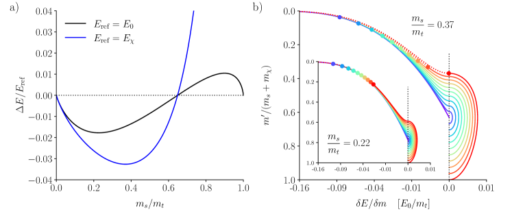
Figure 35: Panel (a): the available energy of a the “two-phase” atmsophere considered in Appendix C, as a function of the mass $m_{s}$ of fluid with $\beta=\infty$. The black line normalizes the available energy by the total initial potential energy, the blue line by the initial potential energy of the fluid with $\beta=0$ only. Panel (b): The energy liberated per unit mass of moving fluid when a slice moves from its initial position to a new location where the supported mass is $m^{\prime}$. The main plot shows the case of $m_{s}/m_{t}=0.37$, which corresponds to the largest possible available energy [minimum of the blue line in Panel (a)]; the inset shows the case of $m_{s}/m_{t}=0.37$, which corresponds to the largest possible fractional available energy [minimum of the black line in Panel (a)].

In this appendix, we consider the simple case of a “two-phase” atmosphere in which a mass $m_{s}$ of fluid with ${\chi=0}$ ($\beta=\infty$) is situated initially below a mass $m_{\mathrm{\chi}}$ of fluid with $s=0$ ($\beta=0$), for which the available energy can be determined analytically. This case is of pedagocial value as it illustrates why the available energy is always a small fraction of the total.

According to Eq. (5), the large-$\beta$ fluid experiences a destabilizing force when displaced upwards into the small-$\beta$ fluid (indeed, the destabilizing force is the greatest possible, as the difference in compressibility is maximal). Intuitively, therefore, we expect the minimum-energy state to be obtainable by re-stacking the atmosphere such that the large-$\beta$ fluid sits above the small-$\beta$ fluid. We consider the most optimistic case from the perspective of available energy — that of an atmosphere initially at marginal linear stability, i.e., $\mathcal{L}=0$ — which means that, by Eq. (4), $s$ and $\chi$ are piecewise-constant functions of $m$:

$$s=\begin{cases}0,&m<m_{\chi},\\ s_{0},&m_{\chi}<m<m_{t},\end{cases}\quad\chi=\begin{cases}\chi_{0},&m<m_{\chi},\\ 0,&m_{\chi}<m<m_{t},\end{cases}$$ (67)

where $m_{t}=m_{s}+m_{\chi}$ is the total mass of the atmosphere. The interface of the two phases at $m=m_{\chi}$ is stable provided the density of the fluid above it is smaller than the density of the fluid below — the case of marginal linear stability is the one where the fluid density is continuous at the interface. By Eq. (11), this implies that

$$\frac{s_{0}}{\chi_{0}}=\frac{1}{\sqrt{2}}(m_{\chi}g)^{1/\gamma-1/2}.$$ (68)

The change in energy $\Delta E$ when the entire mass $m_{s}$ of large-$\beta$ fluid is moved from the bottom to the top may then be shown straightforwardly to satisfy

$$\frac{\Delta E}{E_{\chi}}=C(r^{2-1/\gamma}-(1+r)^{2-1/\gamma}+1)\\ +(1+r)^{3/2}-1-r^{3/2},$$ (69)

where $r=m_{s}/m_{\chi}$, $C=3\gamma^{2}/4(\gamma-1)(2\gamma-1)$ and

$$E_{\chi}=\frac{2}{3}(2m_{\chi}^{3}g)^{1/2}\chi_{c}$$ (70)

is the total energy of the small-$\beta$ fluid at the top of the atmosphere, which is related to the total energy of the atmosphere $E_{0}$ via

$$\frac{E_{0}}{E_{\chi}}=1+C[(1+r)^{2-1/\gamma}-1].$$ (71)

In the limit of $r\to 0$, Eqs. (69) and (71) give

$$\frac{\Delta E}{E_{\chi}}=\frac{\Delta E}{E_{0}}=-\frac{3r}{8}=-\frac{3m_{s}}{8m_{t}}.$$ (72)

Thus, the fractional energy change of a small-$\beta$ atmosphere at marginal linear stability when a small parcel of large-$\beta$ fluid rises through it is proportional to the mass fraction of the fluid moved, with a proportionality factor of order unity. However, returns in the fractional energy change diminish rapidly as the amount of mass moved increases. In Fig. 35(a), we visualise $\Delta E$ normalised by $E_{0}$ (black line) and $E_{\chi}$ (blue line) as a function of the mass fraction $m_{s}/m_{t}$ of large-$\beta$ fluid in the atmosphere. We observe that, despite its order-unity initial gradient of $-3/8$, $\Delta E/E_{0}$ shallows rapidly, reaching a minimum of $-1.8\%$ where the large-$\beta$ fluid has a mass fraction of $22\%$. If the mass fraction of the large-$\beta$ is greater than this, the fractional energy liberated in moving the large-$\beta$ fluid is smaller, and, for a mass fraction of greater than $65\%$, moving the large-$\beta$ fluid incurs an energetic cost.

To elucidate the reason for the diminishing return, we consider the rearrangement as a sequence of displacements of parcels of the large-$\beta$ fluid from just below the interface to new positions at the top of the atmosphere. Fig. 35(b) shows, for a sequence of parcel displacements represented by lines colored from purple (the first parcel to move) to red (the last parcel to move), the energy $\delta E$ that is liberated when a mass $\delta m$ of the large-$\beta$ fluid is moved from the (evolving) position of the interface to a new, smaller, supported mass $m^{\prime}$ (end points of the particle motions are shown as filled circles). The decrease in the magnitude of $\delta E/\delta m$ for subsequent parcels is seen to occur because fluid parcels obey an exclusion principle — two slices cannot have the same supported mass. This means that a parcel of fluid that has already risen from the bottom to the top of the atmosphere will prevent the next parcel from rising to the same height, thus limiting the difference in total pressure that this parcel experiences over its motion, and so reducing the work done on the parcel by the buoyancy force (recall that for an atmosphere at marginal linear stability, the latter is proportional to the ratio of pressures at the initial and final positions).

A second effect visible in Fig. 35(b) is that the motion of the first fluid parcel stabilizes the atmosphere somewhat, because it moves the interface between the large- and small-$\beta$ fluid downwards, where the total pressure is greater (the constants $s_{0}$ and $\chi_{0}$ were chosen such that the large- and small-$\beta$ fluids had the same density at $P=m_{\chi}g$; at larger pressure, the more compressible, large-$\beta$ fluid underneath the interface is denser). The buoyancy force on a rising parcel is downwards (restoring) until it passes the point of neutral buoyancy at the original position of the interface. If the work required to overcome the restoring force is greater than the energy liberated when the parcel moves to the greatest height permitted by the exclusion principle, then the reassignment incurs a net energetic cost. This situation occurs for $m_{s}\gtrsim 0.37m_{t}$: for $m_{s}$ larger than this, $\Delta E/E_{\mathrm{\chi}}$ rises with $m_{s}$ [Fig. 35(a)], becoming positive for $m_{s}\gtrsim 0.65m_{t}$. $\Delta E/E_{0}$ reaches a minimum at smaller $m_{s}/m_{t}$ because the small increase in available energy is outweighed by the energetic cost incurred by increasing the total mass of the atmosphere.

Appendix D A necessary condition for “one-to-many” optimal assignment

We can deduce a necessary condition for the one-to-many optimal assignment described in Section III.3.2 in a similar manner to the one in which we deduced the equal-density condition (31) for “many-to-one” assignments in Section III.3.1. Let us suppose that we are given the optimal assignment of all slices apart from those with initial supported mass $m_{i}=m_{a}+\delta m_{i}$. Their contribution to the total energy of the atmosphere is

$$\delta E =\Delta m\sum_{i}\mathcal{E}(m_{\sigma(i)},m_{a}+\delta m_{i})$$

$$=\Delta m\sum_{i}\bigg{[}\mathcal{E}(m_{\sigma(i)},m_{a})$$

$$\quad+\delta m_{i}\frac{\partial\mathcal{E}}{\partial\mu}(m_{\sigma(i)},m_{a})+\mathcal{O}(\delta m_{i}^{2})\bigg{]}.$$ (73)

where

$$\frac{\partial\mathcal{E}}{\partial\mu}=\frac{1}{\gamma-1}\rho^{\gamma-1}\frac{\mathrm{d}s^{\gamma}}{\mathrm{d}\mu}+\frac{1}{2}\rho\frac{\mathrm{d}\chi^{2}}{\mathrm{d}\mu}.$$ (74)

Thus, a necessary (but not sufficient) condition for the optimal assignment to be one-to-two is that $\partial\mathcal{E}/\partial\mu$ must be equal (up to a difference proportional to $\Delta m$) when evaluated [with ${s=s(\mu)}$ and ${\chi=\chi(\mu)}$] at each of the two different supported masses $m_{\sigma(i)}$ to which slices in the vicinity of $m_{a}$ are to be assigned. If this is not the case for any $\delta m_{i}$ in the given range, then Eq. (73) is minimized to leading order in $\delta m$ by assigning the slice with largest initial supported mass to the new supported mass for which $\partial\mathcal{E}/\partial\mu$ is smallest, and so on — this will always be a one-to-one assignment, as $\partial\mathcal{E}/\partial\mu$ is continuous in $m_{\sigma(i)}$ for fixed $m_{a}$.

Denoting the density of slice $i$ at the two values of $m_{\sigma(i)}$ by $\rho$ and $\rho^{\prime}$, the condition for a one-to-two mapping is [cf. Eq. (31)]

$$\frac{1}{\gamma-1}(\rho^{\prime\gamma-1}-\rho^{\gamma-1})\frac{\mathrm{d}s^{\gamma}}{\mathrm{d}m}+\frac{1}{2}(\rho^{\prime}-\rho)\frac{\mathrm{d}\chi^{2}}{\mathrm{d}m}=\mathcal{O}(\Delta m).$$ (75)

From this expression, we see that, for any given $\rho$, there can be at most one solution for $\rho^{\prime}$ in addition to the trivial $\rho^{\prime}=\rho$. The existence of a second solution requires that gradients of $s$ and $\chi$ with $m$ have opposite signs in the initial profile. Thus, while an optimal assignment may in general be one-to-two, like in Figs. 12, it cannot be one-to-$X$ with ${X>2}$.

Appendix E Lynden-Bell to linear sum assignment: degenerate cases

In cases where $\tilde{\mathcal{E}}$ has zeros that do not form part of the unique optimal assignment, or else has more than one optimal assignment, Eq. (53) becomes

$$P_{ij}\to\frac{1}{\Delta m}\frac{\displaystyle a_{ij}F_{i}}{\displaystyle\sum_{k}a_{kj}F_{k}}\,\,\mathrm{as}\,\,\beta_{T}\to\infty$$ (76)

where $a_{ij}=1$ if $\tilde{\mathcal{E}}_{ij}=0$ and $a_{ij}=0$ otherwise, and ${F_{i}=e^{\beta_{T}\tilde{\psi}_{i}}}$ is the quantity sometimes known as “fugacity” [in writing Eq. (76), we assumed that $\tilde{\psi}_{i}<0$; we were free to do so because taking $\tilde{\psi}_{i}\to\tilde{\psi}_{i}+C$ for all $i$ with $C$ a constant leaves Eq. (52) unchanged]. The values of $F_{i}$ are determined by Eq. (49), which requires that

$$\sum_{j}\frac{\displaystyle a_{ij}F_{i}}{\displaystyle\sum_{k}a_{kj}F_{k}}=1,\quad\forall i,$$ (77)

an equation that may be solved iteratively for $F_{i}$, and hence $P_{ij}$. The possible outcomes of such a procedure are constrained by the Birkhoff-von Neumann theorem, which states that any doubly stochastic matrix — one whose rows and columns all sum to unity — can be expressed as a sum of permutation matrices with positive weights that also sum to unity. From Eqs. (48) and (49), $P_{ij}$ is a doubly stochastic matrix, so that

$$P_{ij}=\frac{1}{\Delta m}\sum_{k}\theta_{k}S^{(k)}_{ij},\quad\theta_{k}>0,\quad\sum_{k}\theta_{k}=1,$$ (78)

where $S^{(k)}_{ij}$ are permutation matrices. In the $\beta_{T}\to\infty$ limit, $P_{ij}\propto a_{ij}$ [Eq. (76)], so $\{S^{(k)}_{ij}\}$ is the maximal set of permutations that vanish wherever $\tilde{\mathcal{E}}_{ij}>0$, which we recognize as the optimal assignments of the LSA problem: with $\sigma^{(k)}$ the $k$th optimal assignment, $S^{(k)}_{ij}$ is the matrix representation of $\sigma^{(k)}$, i.e., $S^{(k)}_{ij}=\delta_{j\sigma^{(k)}(i)}$. It follows that $P_{ij}=0$ for any $ij$ that is not part of an optimal assignment, even if $\tilde{\mathcal{E}}_{ij}=0$, and that

$$E=\Delta m\sum_{ijk}\mathcal{E}_{ij}\theta_{k}S^{(k)}_{ij}=\Delta m\sum_{k}\theta_{k}\sum_{i}\mathcal{E}_{i\sigma^{(k)}(i)}=E_{\mathrm{min}}.$$ (79)

Appendix F Uniqueness of doubly stochastic delta distributions

Figure 36: Visualization of the construction of the delta distribution (80) for the curve $\mathcal{C}$ by solving Eqs. (83). Colored dashed lines indicate the relevant vertical and horizontal lines used in the evaluation of Eqs. (83). For ease of comparison between different parts of $\mathcal{C}$, the gray lines mark certain points at which $\mathcal{C}$ has discontinuities.

In this appendix, we show that the delta distribution

$$\mathcal{P}(x,y)=A(x,y)\delta(F(x,y)),$$ (80)

where $A>0$, and $F(x,y)=0$ on a piecewise-once-differentiable curve $\mathcal{C}$, is unique under the conditions that

1. $\mathcal{C}$ intersects every horizontal and vertical line in the unit square at least once,

2. $\mathcal{C}$ does not admit any cycles formed by traversing horizontal and vertical lines (in the context of Eq. (55), this corresponds to uniqueness of the optimal assignment),

3. $\mathcal{P}(x,y)$ satisfies the integral constraints

   $$\int_{0}^{1}\mathrm{d}x\mathcal{P}(x,y)=1$$ (81)

   and

   $$\int_{0}^{1}\mathrm{d}y\mathcal{P}(x,y)=1.$$ (82)

Without loss of generality, we can take $|\bm{\nabla}F|=1$; any other choice amounts to a redefinition of $A$. Then, Eqs. (81) and (82) become

$$\sum_{i}\frac{A(x_{i}(y),x)}{|t_{x}(x_{i}(y),y)|}=1,\quad\sum_{i}\frac{A(x,y_{i}(x))}{|t_{y}(x,y_{i}(x))|}=1,$$ (83)

respectively, where $y_{i}(x)$ is the $y$-coordinate of the $i$th intersection of $\mathcal{C}$ with the vertical line through ($x$,0), $x_{i}(y)$ is the $x$-coordinate of the $i$th intersection of $\mathcal{C}$ with the horizontal line through $(0,y)$, and

$$(t_{x},t_{y})=\left(\frac{\partial F}{\partial y},-\frac{\partial F}{\partial x}\right)$$ (84)

is the unit tangent vector to $\mathcal{C}$.

For each point on $\mathcal{C}$, Eqs. (83) each provide an equation relating $A$ at that point to the value of $A$ at each other point on $\mathcal{C}$ with the same $x$ or $y$ coordinate. In turn, Eqs. (83) provide one additional equation for each such point of intersection, relating $A$ evaluated there to $A$ evaluated at other points on $\mathcal{C}$ with the same $x$ or $y$-coordinate, and so on for the points with which those points share an $x$ or $y$ coordinate. There are three possible outcomes for this proliferation of coupled equations: (a) a stage of the process is reached when all new equations only involve a single point on $\mathcal{C}$, and so the proliferation is arrested when $n+1$ independent (prior to the specification of the tangent vectors) linear equations couple the values of $A$ at $n$ different points; (b) proliferation of equations ceases, but the $n$ points on $\mathcal{C}$ form one or more cycles of the sort envisioned in (ii) and are therefore coupled by fewer than $n+1$ equations; (c) proliferation of equations never ceases — in this case, infinitely many points are coupled, some of them arbitrarily close to each other (infinite cycle). By condition (ii), we restrict attention to case (a). Then, the first $n$ of the $n+1$ independent linear equations can be solved for the values of $A$ at each of the $n$ points, so the function $A(x,y)$ is indeed unique given conditions (i)-(iii), as claimed. The final equation gives a constraint on the tangent vectors, which must be satisfied in order for a delta distribution (80) satisfying conditions (i)-(iii) to exist.

For clarity, we illustrate the procedure described above for the example curve $\mathcal{C}$ shown in Fig. 36.

F.1 Case where vertical and horizontal lines intersect $\mathcal{C}$ once only — red point in Fig. 36

In this case, Eqs. (83) become

$$\frac{A}{|t_{y}|}=1,\quad\frac{A}{|t_{x}|}=1\implies A=|t_{x}|=|t_{y}|=\frac{1}{\sqrt{2}},$$ (85)

from which it follows that

$$\frac{\mathrm{d}y}{\mathrm{d}x}=\pm 1$$ (86)

must be satisfied at the point in question. As claimed, we find the unique value of $A$ and a condition on the tangent vector.

F.2 Case where one vertical line intersects $\mathcal{C}$ twice — yellow points in Fig. 36

With subscripts indicating evaluation at points according to the labelling scheme in Fig. 36, Eqs. (83) yield

$$\frac{A_{1}}{|t_{y1}|}=1,\quad\frac{A_{2}}{|t_{y2}|}=1,\quad\frac{A_{1}}{|t_{x1}|}+\frac{A_{2}}{|t_{x2}|}=1,$$ (87)

from which it follows that

$$A_{1}=|t_{y2}|,\quad A_{2}=|t_{y2}|,\quad\bigg{|}\frac{\mathrm{d}y}{\mathrm{d}x}\bigg{|}_{1}+\bigg{|}\frac{\mathrm{d}y}{\mathrm{d}x}\bigg{|}_{2}=1.$$ (88)

As claimed, we find the unique values of $A_{1}$ and $A_{2}$ and a condition on the tangent vector at the relevant points.

F.3 Case where one horizontal line intersects $\mathcal{C}$ twice — pink points in Fig. 36

In this case, Eqs. (83) yield

$$\frac{A_{1}}{|t_{x1}|}=1,\quad\frac{A_{2}}{|t_{x2}|}=1,\quad\frac{A_{1}}{|t_{y1}|}+\frac{A_{2}}{|t_{y2}|}=1,$$ (89)

from which it follows that

$$A_{1}=|t_{x2}|,\quad A_{2}=|t_{x2}|,\quad\bigg{|}\frac{\mathrm{d}y}{\mathrm{d}x}\bigg{|}^{-1}_{1}+\bigg{|}\frac{\mathrm{d}y}{\mathrm{d}x}\bigg{|}^{-1}_{2}=1.$$ (90)

Again, we find the unique values of $A_{1}$ and $A_{2}$ and a condition on the tangent vector at the relevant points.

F.4 Case where both one vertical and one horizontal line intersects $\mathcal{C}$ — blue points in Fig. 36

In this case, three points are coupled by Eqs. (83), which yield

$$\frac{A_{2}}{|t_{x2}|}=1,\quad\frac{A_{3}}{|t_{y3}|}=1,\\ \frac{A_{1}}{|t_{x1}|}+\frac{A_{3}}{|t_{x3}|}=1,\quad\frac{A_{1}}{|t_{y1}|}+\frac{A_{2}}{|t_{y2}|}=1,$$ (91)

from which it follows that the values of $A_{i}$ are

$$A_{1}=\left(1-\frac{|t_{x2}|}{|t_{y2}|}\right)|t_{y1}|,\quad A_{2}=|t_{x2}|,\quad A_{3}=|t_{y3}|$$ (92)

and the condition on $\mathcal{C}$ is

$$\bigg{|}\frac{\mathrm{d}y}{\mathrm{d}x}\bigg{|}_{3}=\bigg{|}\frac{\mathrm{d}y}{\mathrm{d}x}\bigg{|}_{1}\left[\bigg{|}\frac{\mathrm{d}y}{\mathrm{d}x}\bigg{|}^{-1}_{1}+\bigg{|}\frac{\mathrm{d}y}{\mathrm{d}x}\bigg{|}_{2}^{-1}-1\right].$$ (93)

F.5 Case in which $\mathcal{C}$ has a simple cycle — green points in Fig. 36

To illustrate how uniqueness fails if condition (ii) is not satisfied, we consider as a final example the case where four points form a cycle along horizontal and vertical lines. Eqs. (83) yield

$$\frac{A_{1}}{|t_{y1}|}+\frac{A_{2}}{|t_{y2}|}=1,\quad\frac{A_{1}}{|t_{x1}|}+\frac{A_{3}}{|t_{x3}|}=1,\\ \frac{A_{3}}{|t_{y3}|}+\frac{A_{4}}{|t_{y4}|}=1,\quad\frac{A_{2}}{|t_{x2}|}+\frac{A_{4}}{|t_{x4}|}=1.$$ (94)

These equations can be reduced to the matrix equation

$$\begin{pmatrix}\displaystyle\frac{1}{|t_{y1}|}&-\displaystyle\frac{|t_{x2}|}{|t_{y2}||t_{x4}|}\vspace{2mm}\\ -\displaystyle\frac{|t_{x3}|}{|t_{y3}||t_{x1}|}&\displaystyle\frac{1}{|t_{y4}|}\end{pmatrix}\begin{pmatrix}A_{1}\\ A_{4}\end{pmatrix}=\begin{pmatrix}1-\displaystyle\frac{|t_{x2}|}{|t_{y2}|}\vspace{2mm}\\ 1-\displaystyle\frac{|t_{x3}|}{|t_{y3}|}\end{pmatrix},$$ (95)

which has unique solutions for $A_{1}$ and $A_{4}$ unless the determinant of the matrix is zero, which requires

$$\bigg{|}\frac{\mathrm{d}y}{\mathrm{d}x}\bigg{|}_{1}\bigg{|}\frac{\mathrm{d}y}{\mathrm{d}x}\bigg{|}_{4}=\bigg{|}\frac{\mathrm{d}y}{\mathrm{d}x}\bigg{|}_{2}\bigg{|}\frac{\mathrm{d}y}{\mathrm{d}x}\bigg{|}_{3}.$$ (96)

In this case, the $A_{i}$ are not determined uniquely. It is straightforwardly verified that Eq. (96) is precisely the condition for the four points separated by an infinitesimal distance along $\mathcal{C}$ from the green ones to also be on a cycle of horizontal and vertical lines. Thus, it appears that condition (ii) is actually too strong a condition to guarantee uniqueness of Eq. (80): cycles are permissible if they only exist in a set of measure zero in $x$ and $y$. It follows that cases where the optimal solution to the assignment problem is non-unique on a set of measure zero only do not violate the conclusion of Section IV.4.

References

- Cranmer and Winebarger [2019] S. R. Cranmer and A. R. Winebarger, The properties of the solar corona and its connection to the solar wind, Annu. Rev. Astron. Astrophys. 57, 157 (2019).
- ITER Physics Expert Group on Confinement and Transport et al. [1999] ITER Physics Expert Group on Confinement and Transport, ITER Physics Expert Group on Confinement Modelling, and ITER Physics Basis Editors, ITER physics basis, chapter 2: Plasma confinement and transport, Nucl. Fusion 39, 2175 (1999).
- Chen [2011] P. F. Chen, Coronal mass ejections: Models and their observational basis, Living Reviews in Sol. Phys. 8, 1 (2011).
- Hender et al. [2007] T. C. Hender, J. C. Wesley, J. Bialek, A. Bondeson, A. H. Boozer, R. J. Buttery, A. Garofalo, T. P. Goodman, R. S. Granetz, Y. Gribov, et al., Progress in the ITER physics basis, chapter 3: MHD stability, operational limits and disruptions, Nucl. Fusion 47, S128 (2007).
- Connor et al. [1979] J. W. Connor, R. J. Hastie, and J. B. Taylor, High mode number stability of an axisymmetric toroidal plasma, Proc. R. Soc. Lond. 365, 1 (1979).
- Cowley and Artun [1997] S. C. Cowley and M. Artun, Explosive instabilities and detonation in magnetohydrodynamics., Phys. Rep. 283, 185 (1997).
- Hurricane et al. [1997] O. A. Hurricane, B. H. Fong, and S. C. Cowley, Nonlinear magnetohydrodynamic detonation: Part I, Phys. Plasmas 4, 3565 (1997).
- Wilson and Cowley [2004] H. R. Wilson and S. C. Cowley, Theory for explosive ideal magnetohydrodynamic instabilities in plasmas, Phys. Rev. Lett. 92, 175006 (2004).
- Cowley et al. [2015] S. C. Cowley, B. Cowley, S. A. Henneberg, and H. R. Wilson, Explosive instability and erupting flux tubes in a magnetized plasma, Proc. R. Soc. Lond. 471, 20140913 (2015).
- Ham et al. [2018] C. J. Ham, S. C. Cowley, G. Brochard, and H. R. Wilson, Nonlinear ballooning modes in tokamaks: stability and saturation, Plasma Phys. Control. Fusion 60, 075017 (2018).
- Schwarzschild [1906] K. Schwarzschild, On the equilibrium of the Sun’s atmosphere, Gottinger Nachr. 195, 41 (1906).
- Stevens [2005] B. Stevens, Atmospheric moist convection, Annu. Rev. Earth Planet. Sci. 33, 605 (2005).
- Hieronymus and Nycander [2015] M. Hieronymus and J. Nycander, Finding the minimum potential energy state by adiabatic parcel rearrangements with a nonlinear equation of state: an exact solution in polynomial time, J. Phys. Oceanogr. 45, 1843 (2015).
- Su and Ingersoll [2016] Z. Su and A. P. Ingersoll, On the minimum potential energy state and the eddy size-constrained APE density, J. Phys. Oceanogr. 46, 2663 (2016).
- Stansifer et al. [2017] E. M. Stansifer, P. A. O’Gorman, and J. I. Holt, Accurate computation of moist available potential energy with the Munkres algorithm, Quarterly Journal of the Royal Meteorological Society 143, 288 (2017).
- Lynden-Bell [1967] D. Lynden-Bell, Statistical mechanics of violent relaxation in stellar systems, Mon. Not. R. Astron. Soc. 136, 101 (1967).
- Miller [1990] J. Miller, Statistical mechanics of Euler equations in two dimensions, Phys. Rev. Lett. 65, 2137 (1990).
- Miller et al. [1992] J. Miller, P. B. Weichman, and M. C. Cross, Statistical mechanics, Euler’s equation, and Jupiter’s Red Spot, Phys. Rev. A 45, 2328 (1992).
- Robert [1991] R. Robert, A maximum-entropy principle for two-dimensional perfect fluid dynamics, J. Stat. Phys. 65, 531 (1991).
- Robert and Sommeria [1991] R. Robert and J. Sommeria, Statistical equililbrium states for two-dimensional flows, J. Fluid Mech. 229, 291 (1991).
- Singh and O’Neill [2022] M. S. Singh and M. E. O’Neill, The climate system and the second law of thermodynamics, Rev. Mod. Phys. 94, 015001 (2022).
- Hughes and Brummell [2021] D. W. Hughes and N. H. Brummell, Double-diffusive magnetic layering, Astrophys. J. 922, 195 (2021).
- Landau and Lifshitz [1959] L. D. Landau and E. M. Lifshitz, Fluid Mechanics (Pergamon Press, 1959).
- Lorenz [1955] E. N. Lorenz, Available potential energy and the maintenance of the general circulation, Tellus 7, 157 (1955).
- Burkard et al. [2012] R. Burkard, M. Dell’Amico, and S. Martello, Assignment Problems (Society for Industrial and Applied Mathematics, 2012).
- Munkres [1957] J. Munkres, Algorithms for the assignment and transportation problems, J. Soc. Ind. Appl. Math. 5, 32 (1957).
- Kuhn [1955] H. W. Kuhn, The hungarian method for the assignment problem, Nav. Res. Logist. Quart. 2, 83 (1955).
- Chavanis [2003] P. H. Chavanis, Gravitational instability of isothermal and polytropic spheres, Astron. Astrophys. 401, 15 (2003).
- Ewart et al. [2023] R. J. Ewart, M. L. Nastac, and A. A. Schekochihin, Non-thermal particle acceleration and power-law tails via relaxation to universal Lynden-Bell equilibria, J. Plasma Phys. 89, 905890516 (2023).
- Kirk et al. [2004] A. Kirk, H. R. Wilson, G. F. Counsell, R. Akers, E. Arends, S. C. Cowley, J. Dowling, B. Lloyd, M. Price, and M. Walsh, Spatial and temporal structure of edge-localized modes, Phys. Rev. Lett. 92, 245002 (2004).
- Kirk et al. [2006] A. Kirk, B. Koch, R. Scannell, H. R. Wilson, G. Counsell, J. Dowling, A. Herrmann, R. Martin, and M. Walsh, Evolution of filament structures during edge-localized modes in the MAST tokamak, Phys. Rev. Lett. 96, 185001 (2006).
- Taylor [1974] J. B. Taylor, Relaxation of toroidal plasma and generation of reverse magnetic fields, Phys. Rev. Lett. 33, 1139 (1974).
- Taylor [1986] J. B. Taylor, Relaxation and magnetic reconnection in plasmas, Rev. Mod. Phys. 58, 741 (1986).
- Zhou et al. [2019] M. Zhou, P. Bhat, N. F. Loureiro, and D. A. Uzdensky, Magnetic island merger as a mechanism for inverse magnetic energy transfer, Phys. Rev. Res. 1, 012004 (2019).
- Bhat et al. [2021] P. Bhat, M. Zhou, and N. F. Loureiro, Inverse energy transfer in decaying, three-dimensional, non-helical magnetic turbulence due to magnetic reconnection, Mon. Not. R. Astron. Soc. 501, 3074 (2021).
- Hosking and Schekochihin [2021] D. N. Hosking and A. A. Schekochihin, Reconnection-controlled decay of magnetohydrodynamic turbulence and the role of invariants, Phys. Rev. X 11, 041005 (2021).
- Merryfield [2000] W. J. Merryfield, Origin of thermohaline staircases, J. Phys. Oceanogr. 30, 1046 (2000).
- Pencil Code Collaboration et al. [2021] Pencil Code Collaboration, A. Brandenburg, A. Johansen, P. Bourdin, W. Dobler, W. Lyra, M. Rheinhardt, S. Bingert, N. Haugen, et al., The Pencil Code, a modular MPI code for partial differential equations and particles: multipurpose and multiuser-maintained, J. Open Source Softw. 6, 2807 (2021).
- Hughes [1985] D. W. Hughes, Magnetic buoyancy instabilities for a static plane layer, Geophys. Astrophys. Fluid Dyn. 32, 273 (1985).