Mixed QCD-EW corrections to $W$-pair production at electron-positron colliders

Abstract

The discrepancy between the CDF measurement and the Standard Model theoretical predictions for the $W$-boson mass underscores the importance of conducting high-precision studies on the $W$ boson, which is one of the predominant objectives of proposed future $e^{+}e^{-}$ colliders. We investigate in detail the production of $W$-boson pair at $e^{+}e^{-}$ colliders and calculate the mixed QCD-EW corrections at the next-to-next-to-leading order. By employing the method of differential equations, we analytically compute the two-loop master integrals for the mixed QCD-EW corrections to $e^{+}e^{-}\to W^{+}W^{-}$. By utilizing the Magnus transformation, we derive a canonical set of master integrals for each integral family. This canonical basis fulfills a system of differential equations where the dependence on the dimensional regulator, $\epsilon$, is linearly factorized from the kinematics. Finally, these canonical master integrals are given as Taylor series in $\epsilon$ up to $\epsilon^{4}$, with coefficients written as combinations of Goncharov polylogarithms up to weight four. Upon applying our analytic expressions of these master integrals to the phenomenological analysis on $W$-pair production, we find that the $\mathcal{O}(\alpha\alpha_{s})$ corrections hold substantial significance in the $\alpha(0)$ scheme, especially in the vicinity of the top-pair resonance ($\sqrt{s}=2\,m_{t}$) induced by top-loop integrals. However, these corrections can be heavily suppressed by adopting the $G_{\mu}$ scheme.

1 Introduction

The discovery of the Higgs boson ATLAS:2012yve ; CMS:2012qbp at the CERN Large Hadron Collider (LHC) in 2012 marked a pivotal moment in the field of elementary particle physics, validating the last missing piece of the Standard Model (SM). However, the CDF collaboration recently announced a high-precision measurement of the $W$-boson mass CDF:2022hxs ,

$$m_{\scriptscriptstyle{W}}^{\scriptscriptstyle{\text{CDF}}}=80.4335\pm 0.0094~{}\mathrm{GeV}\,,$$ (1)

indicating a significant $7\sigma$ deviation from the SM prediction. This deviation raises questions about the internal consistency of the SM. To address this anomaly between experimental measurements and theoretical predictions, a profound and comprehensive understanding of the SM, particularly the gauge structure of the electroweak (EW) sector, becomes imperative. Therefore, the pursuit of high-precision experimental measurements and refined theoretical calculations within the framework of the SM stands as a paramount objective in the contemporary and future high-energy physics research.

The $W$-boson pair production at $e^{+}e^{-}$ colliders offers a direct avenue for measuring the $W$-boson mass, since the production cross section around the threshold exhibits a high sensitivity to the $W$-boson mass. Furthermore, this process serves as an ideal platform for investigating the electroweak symmetry breaking mechanism, as it directly unveils the intricate structure of triple gauge-boson interactions Bilenky:1993ms ; Gounaris:1996rz . Remarkably, the total cross section of $W$-pair production has been measured with an impressive accuracy of $\sim 1\%$, and the determination of the $W$-boson mass has reached a precision of $33~{}\mathrm{MeV}$, achieved through a combination of direct reconstruction and threshold measurements at LEP2 ALEPH:2013dgf . Future advancements in precision measurements of the $W$-boson mass and the total cross section of $W$-pair production are anticipated. These endeavors have been proposed by next-generation high-luminosity $e^{+}e^{-}$ collider projects,including the International Linear Collider (ILC) Behnke:2013xla ; ILC:2013jhg ; Bambade:2019fyw , the Circular Electron-Positron Collider (CEPC) CEPCStudyGroup:2018rmc ; CEPCStudyGroup:2018ghi and the Future Circular Collider (FCC-ee) FCC:2018byv ; FCC:2018evy . Notably, these initiatives aim to measure the $W$-boson mass with extraordinary precision, achieving an accuracy of just a few $\mathrm{MeV}$ at ILC ILC:2013jhg , $1~{}\mathrm{MeV}$ at CEPC CEPCStudyGroup:2018ghi and $0.5~{}\mathrm{MeV}$ at FCC-ee FCC:2018evy , which surpass the precision of the CDF measurement.

In anticipation of the upcoming high-precision experimental measurements, it becomes imperative to attain an extremely fine level of control over the theoretical prediction for the $W$-pair production cross section, reaching the permille (or even sub-permille) level. The process of $e^{+}e^{-}\to W^{+}W^{-}$ has been detailedly studied at LEP, with particular focus on measuring the $W$ helicity and exploring the impact of beam polarization Blondel:1987pm . The complete next-to-leading order (NLO) electroweak $\mathcal{O}(\alpha)$ corrections to $e^{+}e^{-}\to W^{+}W^{-}$, comprising virtual one-loop electroweak correction, real-photon radiation correction, and initial-state radiation (ISR) leading logarithmic (LL) QED correction, have been calculated in the past few decades Alles:1976qv ; Hagiwara:1986vm ; Lemoine:1979pm ; Philippe:1981up ; Bohm:1987ck ; Beenakker:1990sf ; Beenakker:1991jk ; Fleischer:1988kj ; Kolodziej:1991pk ; Fleischer:1991nw ; Beenakker:1994vn ; Zerwas:1991rrh . For more comprehensive overviews, please refer to refs. Denner:1991kt ; Beenakker:1996kt . In spite of the remarkable precision achieved by NLO EW theoretical predictions, often reaching accuracy levels of a few percentage points or even sub-percent levels, it is expected that the experimental measurements at forthcoming facilities such as ILC, CEPC, and FCC-ee will surpass this level of accuracy. In order to align with the anticipated permille accuracy of the cross-section measurements at future lepton colliders, it is essential to delve into higher-order corrections in our theoretical predictions. The next-to-next-to-leading order (NNLO) corrections to EW processes are composed of the pure EW $\mathcal{O}(\alpha^{2})$ corrections and the mixed QCD-EW $\mathcal{O}(\alpha\alpha_{s})$ corrections. Calculating the EW $\mathcal{O}(\alpha^{2})$ corrections presents an exceptional challenge due to the tremendous number of two-loop Feynman diagrams involved in the virtual corrections. In contrast, the mixed NNLO QCD-EW corrections prove to be more tractable and may possess greater magnitude owning to the large QCD strong coupling constant. In light of these considerations, this paper focuses on a comprehensive investigation into the $\mathcal{O}(\alpha\alpha_{s})$ corrections to the $W$-pair production cross section at lepton colliders. This endeavor represents the most refined and precise theoretical prediction to date.

The mixed QCD-EW $\mathcal{O}(\alpha\alpha_{s})$ corrections to $e^{+}e^{-}\to W^{+}W^{-}$ arises from the interference between LO and $\text{QCD}\otimes\text{EW}$ NNLO amplitudes. These corrections can be categorized into two classes: vertex corrections and self-energy corrections. It is noteworthy that the NNLO $\text{QCD}\otimes\text{EW}$ corrections to $e\nu_{e}W$, $ee\gamma$ and $eeZ$ vertices are solely contributed by their respective $\mathcal{O}(\alpha\alpha_{s})$ counterterms. In this paper, we embark on an analytical journey to calculate the two-loop Feynman integrals appearing in the $\text{QCD}\otimes\text{EW}$ NNLO amplitude. We subsequently apply these analytic results to obtain the NNLO QCD-EW corrected integrated and differential cross sections. Of particular significance is our comprehensive treatment of the complete analytic calculation of the two-loop triangle master integrals (MIs) for triple gauge-boson vertex corrections, which originate from a gluon dressed quark loop of an $SU(2)_{L}$ doublet, comprising two distinct massive flavors. It is pertinent to mention that the MIs for the massless flavors and scenarios with only one massive flavor in the quark loops have been elucidated in refs. Usyukina:1994iw ; Birthwright:2004kk ; Chavez:2012kn ; DiVita:2017xlr ; Ma:2021cxg .

The rest of this paper is organized as follows. In section 2, we begin by establishing our notations for the calculation of $e^{+}e^{-}\to W^{+}W^{-}$, and proceed to delve into the details of the NLO EW corrections and the NNLO $\text{QCD}\otimes\text{EW}$ corrections. Section 3 is dedicated to the analytic calculation of the MIs essential for the mixed QCD-EW two-loop corrections to the triple gauge couplings (TGCs) $VWW~{}(V=\gamma,Z)$. We elaborate on the construction and the solution of the canonical differential equations, as well as the analytic continuation of the MIs. Leveraging the analytic expressions of the MIs derived in section 3, we calculate the production cross section and some kinematic distributions for $e^{+}e^{-}\to W^{+}W^{-}$ at the $\text{QCD}\otimes\text{EW}$ NNLO in both $\alpha(0)$ and $G_{\mu}$ schemes. The numerical results and an in-depth discussion are provided in section 4. Finally, a brief summary is given in section 5.

2 Descriptions of perturbative calculations

In this paper, our focus centers on the calculation of the mixed QCD-EW two-loop corrections to the scattering process

$$e^{+}(p_{1},\lambda_{1})+e^{-}(p_{2},\lambda_{2})\rightarrow W^{+}(p_{3},\lambda_{3})+W^{-}(p_{4},\lambda_{4})\,,$$ (2)

where $p_{1}^{2}=p_{2}^{2}=0$, $p_{3}^{2}=p_{4}^{2}=m_{\scriptscriptstyle{W}}^{2}$, and the electron mass is consistently neglected wherever feasible. Here, $\lambda_{1,2}$ denote the helicities of the initial-state positron and electron, and $\lambda_{3,4}$ represent the polarizations of the final-state $W$ bosons. The Mandelstam invariants for this $2\rightarrow 2$ scattering process are defined by

$$\left\{~{}\begin{aligned} &s=(p_{1}+p_{2})^{2}=4E^{2}\\ &t=(p_{1}-p_{3})^{2}=m_{\scriptscriptstyle{W}}^{2}-2E^{2}(1-\beta\cos\theta)\\ &u=(p_{1}-p_{4})^{2}=m_{\scriptscriptstyle{W}}^{2}-2E^{2}(1+\beta\cos\theta)\end{aligned}\right.$$ (3)

with $E$ denoting the beam energy, $\theta$ characterizing the scattering angle between $e^{+}$ and $W^{+}$, and $\beta=(1-m_{\scriptscriptstyle{W}}^{2}/E^{2})^{1/2}$ signifying the velocity of the $W$ bosons in the center-of-mass (CM) frame. Then the unpolarized differential cross section in the CM frame is given by

$$\frac{\mathrm{d}\sigma}{\mathrm{d}\Omega}=\frac{\beta}{64\pi^{2}s}\frac{1}{4}\sum_{\lambda_{1,\ldots,4}}\big{|}\mathcal{M}(s,t,\lambda_{1,\ldots,4})\big{|}^{2}\,.$$ (4)

2.1 NLO EW corrections

There are two dominant channels for the $W$-pair production at electron-positron colliders: (1) The $t$ channel via $\nu_{e}$ exchange, which contributes exclusively from the left-handed electrons. (2) The $s$ channel via $\gamma$ or $Z$ exchange, which give contributions from both left-handed and right-handed electrons. It is important to note that the contribution from the Higgs exchange is entirely disregarded due to the exceedingly small Yukawa coupling involved. Several representative Feynman diagrams for $e^{+}e^{-}\to W^{+}W^{-}$ at LO and NLO are depicted in figure 1.

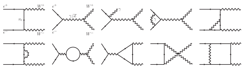
Figure 1: Representative Feynman diagrams for $e^{+}e^{-}\to W^{+}W^{-}$ at LO and NLO. The first two Feynman diagrams belong to LO, the third diagram illustrates the real photon radiation, the rest diagrams depict the one-loop virtual $\mathcal{O}(\alpha)$ corrections.

The essential features of $W$-pair production are determined by the Born cross section. In the threshold region ($\beta\ll 1$), the unpolarized integrated cross section in the Born approximation is given by Denner:1991kt

$$\sigma_{\text{Born}}=\frac{\pi\alpha^{2}}{s}\frac{1}{\sin^{2}\theta_{W}}\beta+\mathcal{O}(\beta^{3})\,.$$ (5)

The leading term proportional to $\beta$ originates from the $t$ channel only, resulting in a threshold behaviour that the cross section is highly sensitive to the exact value of the $W$ mass. Conversely, the contributions from the $s$ channel and the $s$-$t$ interference become proportional to $\beta^{3}$, and thus negligible near the threshold compared to the $s$-channel contribution. In high-energy region, effects of TGCs from the $s$ channel become more apparent, particularly at large scattering angles. Furthermore, we can study a pure TGC process by using right-handed polarized electrons, despite the fact that the right-handed cross section is suppressed compared to the dominant left-handed mode. For more details on LO behaviour, please refer to refs. Alles:1976qv ; Hagiwara:1986vm ; Denner:1991kt ; Beenakker:1994vn ; Beenakker:1996kt .

The complete $\mathcal{O}(\alpha)$ corrections comprise two components: virtual one-loop correction and real photon radiation correction. Moreover, it is essential to account for the ISR effect, which can be implemented in the LL approximation. In our NLO calculation, we adopt the ’t Hooft-Feynman gauge and the on-shell (OS) renormalization scheme Denner:1991kt ; Denner:2019vbn . The ultraviolet (UV) divergences from loop amplitude are regularized by dimensional regularization (DR) scheme in $d=4-2\epsilon$ dimensions, and can be cancelled after performing the renormalization procedure. Infrared (IR) singularities induced by the virtual photon in loops are isolated by an infinitesimal fictitious photon mass. Further consideration of the contributions from real photon radiation ensures the cancellation of the IR divergences. To handle the IR singularities arising from real photon radiation, we employ the two cutoff phase space slicing methods Dittmaier:1999mb ; Denner:2000bj . It is worth noting that all our results have been verified the correctness with the Catani-Seymour dipole subtraction scheme Denner:2000bj . Additionally, the ISR LL QED corrections can be expressed as a convolution of the Born cross section with structure functions Beenakker:1996kt ; Denner:2000bj .

The $\mathcal{O}(\alpha)$ real photon radiation correction to the cross section can be decomposed as

$$\sigma_{\mathrm{real}}=\sigma_{\scriptscriptstyle\mathrm{S}}(\delta_{s})+\sigma_{\scriptscriptstyle\mathrm{HC}}(\delta_{s},\delta_{c})+\sigma_{\scriptscriptstyle\mathrm{H\bar{C}}}(\delta_{s},\delta_{c})\,,$$ (6)

where $\mathrm{S},\,\mathrm{HC},$ and $\mathrm{H\bar{C}}$ denote the contributions of soft, hard-collinear, and hard-noncollinear parts from real photon radiation, respectively. Here, two cutoff parameters, $\delta_{s}$ and $\delta_{c}$, are introduced to address the IR singularities. In our calculation, we verified the cutoff independence of the real photon radiation correction within the range of $\delta_{s}=\delta_{c}\in[10^{-6},10^{-2}]$. Moreover, the ISR LL QED correction is described by the following convolution formula:

$$\sigma_{\scriptscriptstyle\mathrm{ISR-LL}}=\int_{0}^{1}\mathrm{d}x_{1}\mathrm{d}x_{2}\Gamma_{ee}^{\mathrm{LL}}(x_{1},Q^{2})\Gamma_{ee}^{\mathrm{LL}}(x_{2},Q^{2})\int\mathrm{d}\sigma_{0}(x_{1}p_{1},x_{2}p_{2})\,,$$ (7)

where $x_{1}$ and $x_{2}$ represent the fractions of the longitudinal momenta carried by the initial-state leptons after photon radiation, and the typical scale of the hard scattering process, $Q^{2}$, is chosen as $s$. The LL structure function $\Gamma_{ee}^{\mathrm{LL}}$, specified explicitly up to $\mathcal{O}(\alpha^{3})$, is given in refs. Beenakker:1994vn ; Denner:2000bj . To avoid double counting, we must subtract the Born-level cross section and the one-photon emission correction from the ISR contribution. Thus, the higher-order (h.o.ISR) correction can be expressed as

$$\sigma_{\scriptscriptstyle\mathrm{h.o.ISR}}=\sigma_{\scriptscriptstyle\mathrm{ISR-LL}}-\sigma_{\scriptscriptstyle\mathrm{LL,1}}\,,$$ (8)

where the subtraction term $\sigma_{\scriptscriptstyle\mathrm{LL,1}}$ is given by

$$\sigma_{\scriptscriptstyle\mathrm{LL},1}=\int_{0}^{1}\mathrm{d}x_{1}\mathrm{d}x_{2} \Big{[}\delta(1-x_{1})\delta(1-x_{2})+\Gamma_{\mathrm{ee}}^{\mathrm{LL},1}(x_{1},Q^{2})\delta(1-x_{2})$$

$$+\delta(1-x_{1})\Gamma_{\mathrm{ee}}^{\mathrm{LL},1}(x_{2},Q^{2})\Big{]}\int\mathrm{d}\sigma_{0}(x_{1}p_{1},x_{2}p_{2})\,.$$ (9)

Finally, the EW correction is defined as the collective sum of virtual one-loop correction, real photon radiation correction and h.o.ISR correction,

$$\Delta\sigma_{\scriptscriptstyle\mathrm{EW}}=\sigma_{\mathrm{virtual}}+\sigma_{\mathrm{real}}+\sigma_{\scriptscriptstyle\mathrm{h.o.ISR}}\,.$$ (10)

Particular attention must be directed towards the charge renormalization constant. The fine structure constant is defined from the full $ee\gamma$ coupling for on-shell external particles in the Thomson limit, i.e., for a vanishing photon momentum, referred to as the $\alpha(0)$ scheme. In this scheme, the charge renormalization constant is given by

$$\delta Z_{e}|_{\alpha(0)}=-\frac{1}{2}\delta Z_{\gamma\gamma}-\frac{s_{W}}{c_{W}}\frac{1}{2}\delta Z_{Z\gamma}=\frac{1}{2}\Pi^{\gamma\gamma}(0)-\frac{s_{\scriptscriptstyle W}}{c_{\scriptscriptstyle W}}\frac{\Sigma_{\mathrm{T}}^{\gamma Z}(0)}{m_{\scriptscriptstyle Z}^{2}}\,,$$ (11)

which contains mass-singular terms $\log(m^{2}_{f}/\mu^{2})~{}(f=e,\mu,\tau,u,d,c,s,b)$. Significantly, for the QED couplings with external photons, the large logarithms from the electric charge renormalization constant can be cancelled exactly by those from the wave-function renormalization constant of the external photon in the $\alpha(0)$ scheme. For other EW couplings, the mass-singular terms of $\delta Z_{e}|_{\alpha(0)}$ can be absorbed into the running fine structure constant by using the $G_{\mu}$ scheme, wherein the fine structure constant is derived from the Fermi constant $G_{\mu}$ through the following relation:

$$\alpha_{\scriptscriptstyle G_{\mu}}=\frac{\sqrt{2}G_{\mu}m_{\scriptscriptstyle W}^{2}}{\pi}\Big{(}1-\frac{m_{\scriptscriptstyle W}^{2}}{m_{\scriptscriptstyle Z}^{2}}\Big{)}\,.$$ (12)

The corresponding charge renormalization constant is replaced with

$$\delta Z_{e}|_{G_{\mu}}=\delta Z_{e}|_{\alpha(0)}-\frac{1}{2}\Delta r\,,$$ (13)

where $\Delta r$ comprises the higher-order corrections to muon decay Sirlin:1980nh , which can be written as

$$\Delta r=\frac{\partial\Sigma_{\mathrm{T}}^{\gamma\gamma}(k^{2})}{\partial k^{2}}\Big{|}_{k^{2}=0}-2\frac{\delta s_{\scriptscriptstyle W}}{s_{\scriptscriptstyle W}}+2\frac{c_{\scriptscriptstyle W}}{s_{\scriptscriptstyle W}}\frac{\Sigma_{\mathrm{T}}^{\gamma Z}(0)}{m_{\scriptscriptstyle Z}^{2}}+\frac{\Sigma_{\mathrm{T}}^{WW}(0)-\operatorname{Re}\Sigma_{\mathrm{T}}^{WW}(m_{\scriptscriptstyle W}^{2})}{m_{\scriptscriptstyle W}^{2}}+\delta r\,.$$ (14)

Additionally, the $\mathcal{O}(\alpha)$ contribution to the finite remainder, $\delta r$, is

$$\delta r=\frac{\alpha(0)}{4\pi s_{\scriptscriptstyle W}^{2}}\Big{(}6+\frac{7-4s_{\scriptscriptstyle W}^{2}}{2s_{\scriptscriptstyle W}^{2}}\mathrm{ln}c_{\scriptscriptstyle W}^{2}\Big{)}\,.$$ (15)

For comparative purposes, we also conduct calculation in the $\alpha(0)$ scheme.

To compute the EW corrections to $e^{+}e^{-}\to W^{+}W^{-}$, we harness the capabilities of the modified FeynArts, FormCalc, and LoopTools packages Hahn:2000kx ; vanOldenborgh:1990yc ; Hahn:1998yk . These tools play a pivotal role in our calculations. We achieve remarkable agreement, surpassing even the permille level, when comparing our results to the integrated cross-section values provided in refs. Denner:1991kt ; Beenakker:1996kt .

2.2 NNLO mixed QCD-EW corrections

The mixed QCD-EW $\mathcal{O}(\alpha\alpha_{s})$ corrections to $e^{+}e^{-}\to W^{+}W^{-}$ comprise the $e\nu_{e}W$ vertex correction, $eeV$ vertex correction, $\gamma/Z$ self-energy correction, and $VWW$ vertex correction. The representative Feynman diagrams for distinct $\mathcal{O}(\alpha\alpha_{s})$ corrections are depicted in figure 2. The first two types of corrections solely originate from the $\mathcal{O}(\alpha\alpha_{s})$ counterterm, rendering them UV-finite. However, the latter two types of corrections encompass the corrections from the two-loop diagrams that involve attaching one gluon to each one-loop quark line in all possible ways. These corrections also include, one-loop diagrams with insertions of one-loop $\mathcal{O}(\alpha_{s})$ quark mass counterterm, and the $\mathcal{O}(\alpha\alpha_{s})$ counterterm. Therefore, the $\mathcal{O}(\alpha\alpha_{s})$ corrections to the amplitude can be decomposed as

$$\delta\mathcal{M}^{\mathcal{O}(\alpha\alpha_{s})}=\delta\mathcal{M}^{\mathcal{O}(\alpha\alpha_{s})}_{\scriptscriptstyle{e\nu_{e}W}}+\delta\mathcal{M}^{\mathcal{O}(\alpha\alpha_{s})}_{\scriptscriptstyle{eeV}}+\delta\mathcal{M}^{\mathcal{O}(\alpha\alpha_{s})}_{\scriptscriptstyle{\gamma/Z\mbox{-}\mathrm{S.E.}}}+\delta\mathcal{M}^{\mathcal{O}(\alpha\alpha_{s})}_{\scriptscriptstyle{VWW}}\,,$$ (16)

and the corresponding mixed QCD-EW $\mathcal{O}(\alpha\alpha_{s})$ corrections to the cross section can be expressed as

$$\frac{\mathrm{d}\sigma_{\scriptscriptstyle\mathrm{QCD\mbox{-}EW}}}{\mathrm{d}\Omega}=\frac{\beta}{64\pi^{2}s}\frac{1}{4}\sum_{\lambda_{1},\dots,\lambda_{4}}2\operatorname{Re}\Big{|}\mathcal{M}_{0}^{*}(s,t,\lambda_{1},\dots,\lambda_{4})\delta\mathcal{M}^{\mathcal{O}(\alpha\alpha_{s})}(s,t,\lambda_{1},\dots,\lambda_{4})\Big{|}\,.$$ (17)

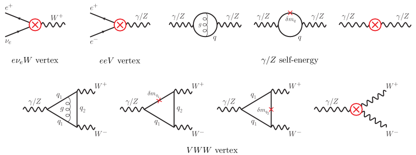
Figure 2: Representative Feynman diagrams for the mixed QCD-EW $\mathcal{O}(\alpha\alpha_{s})$ corrections to $e^{+}e^{-}\to W^{+}W^{-}$. The red cross symbolizes the mass renormalization constant at $\mathcal{O}(\alpha_{s})$, whereas the red circle cross signifies the renormalization constants at $\mathcal{O}(\alpha\alpha_{s})$.

The counterterm contributions to the mixed QCD-EW corrections are comprised of the one-loop $\mathcal{O}(\alpha_{s})$ quark mass counterterm and the two-loop $\mathcal{O}(\alpha\alpha_{s})$ counterterm, as illustrated in figure 2. The quark mass counterterm used in the OS scheme is given by Bernreuther:2004ih

$$\delta m_{q}=-m_{q}\frac{\alpha_{s}}{2\pi}C(\epsilon)\Big{(}\frac{\mu^{2}}{m_{q}^{2}}\Big{)}^{\epsilon}\frac{C_{F}}{2}\frac{3-2\epsilon}{\epsilon(1-2\epsilon)}\,,$$ (18)

where $C(\epsilon)=(4\pi)^{\epsilon}\Gamma(1+\epsilon)$ and $C_{F}=4/3$. The explicit expressions for the $\mathcal{O}(\alpha\alpha_{s})$ counterterms are derived from the NLO EW counterterms Denner:1991kt by replacing the one-loop vector boson self-energies with their two-loop $\mathcal{O}(\alpha\alpha_{s})$ counterpart Dittmaier:2015rxo , which has been well documented in refs. Chang:1981qq ; Djouadi:1987gn ; Djouadi:1987di ; Kniehl:1988ie ; Kniehl:1989yc ; Djouadi:1993ss . Notably, we can confidently disregard the lepton wave-functions counterterms since the lepton self-energies remain unaffected by gluon dressing. Additionally, in the $G_{\mu}$ scheme, contributions to $\Delta r$ in eq. (14) at $\mathcal{O}(\alpha\alpha_{s})$ are streamlined, thanks to the vanishing finite remainder $\delta r$ and the vanishing self-energy $\Sigma_{\mathrm{T}}^{\gamma Z}$ at zero momentum. Once all the contributions at $\mathcal{O}(\alpha\alpha_{s})$ are accounted for, all UV divergences are meticulously cancelled.

In our computational journey of NNLO mixed QCD-EW corrections, we employ the FeynArts package for generating the Feynman diagrams and their corresponding amplitudes. Utilizing an in-house implementation of Mathematica code based on FeynCalc Mertig:1990an ; Shtabovenko:2020gxv , these two-loop amplitudes are manipulated and further expressed as linear combinations of tremendous scalar Feynman integrals, that can be categorized into several families. The Feynman integrals belonging to a given integral family are interrelated and not independent, hence can be further reduced into a small set of irreducible MIs through the utilization of integration-by-parts (IBP) identities Tkachov:1981wb ; Chetyrkin:1981qh . IBP reduction can be facilitated by harnessing the capabilities of publicly available packages, such as Kira Maierhofer:2017gsa ; Klappert:2020nbg , FIRE Smirnov:2019qkx , LiteRed Lee:2012cn ; Lee:2013mka , FiniteFlow Peraro:2019svx , and NeatIBP Wu:2023upw . In our practical endeavors, we mainly employ Kira to conduct IBP reductions, wherein the Laporta algorithm Laporta:2000dsw are implemented for solving IBP identities. Subsequently, we derive the two-loop MIs from the TGC vertices and self-energies after IBP reduction, which are the primary focus of our calculation. A portion of these MIs from the TGC vertices, in combination with all MIs stemming from the self-energies and renormalization constants, can be found in refs. Djouadi:1993ss ; Usyukina:1994iw ; DiVita:2017xlr . However, the remaining two-loop triangle MIs, mediated by two distinct massive flavors quarks in the loops, introduce multiple scales and pose a significant challenge for analytic calculation, hence remain unknown. In our computation, we opt to neglect all quark masses except those of the top quark and bottom quark. We analytically calculate all two-loop MIs appearing in the self-energies and the TGC vertices using the canonical differential equation method Henn:2013pwa ; Henn:2014qga . Additionally, to ensure the accuracy and reliability of our results, all MIs have been cross-checked utilizing numerical tools pySecDec Borowka:2017idc ; Borowka:2018goh and AMFlow Liu:2022chg with high precision. Comprehensive elaboration and further details of our analytic calculation for two-loop triangle MIs, involved in the $\mathcal{O}(\alpha\alpha_{s})$ corrections to $e^{+}e^{-}\to W^{+}W^{-}$ are expounded in the subsequent section.

3 Canonical differential equations

In this section, we commence by establishing the notations and conventions crucial for the calculation of two-loop MIs. Then, we then provide a concise overview of the general structure of canonical differential equations. Following this, we delve into the construction and solutions of the canonical system tailored to our specific process. Lastly, we expound upon the analytic continuation of these MIs.

Our primary focus centers on the analytic calculation of the two-loop MIs arising from the mixed QCD-EW corrections to TGC vertices,

$$V^{*}(p_{3}+p_{4})\to W^{+}(p_{3})+W^{-}(p_{4})\,,$$ (19)

where $V^{*}(p_{3}+p_{4})$ represents the off-shell neutral gauge boson with squared momentum equal to $s$, while both $W$ bosons are on-shell. The two-loop Feynman diagrams relevant for the $\mathcal{O}(\alpha\alpha_{s})$ corrections to $VWW$ vertices can be categorized into three top-level topologies, as visually depicted in figure 3.

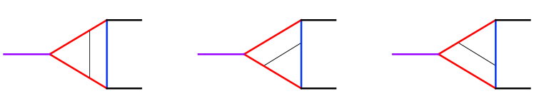
Figure 3: Depiction of three top-level two-loop topologies contributing to the mixed QCD-EW corrections to $VWW$ TGCs. The thin line denotes massless propagators, while the red and blue thick lines symbolize massive propagators with $m_{t}$ and $m_{b}$, respectively. The purple external line corresponds to the off-shell leg with squared momentum equal to $s$, whereas the black thick external lines signify the on-shell external $W$ bosons with mass $m_{\scriptscriptstyle W}$.

For our calculations, we evaluate the two-loop Feynman integrals in $d=4-2\epsilon$ dimensions of the form

$$F(\alpha_{1},\dots,\alpha_{7})=\int\mathcal{D}^{d}l_{1}\mathcal{D}^{d}l_{2}\frac{1}{D_{1}^{\alpha_{1}}\dots D_{7}^{\alpha_{7}}}\,,$$ (20)

where the integration measure defined as

$$\mathcal{D}^{d}l_{i}=\frac{d^{d}l_{i}}{(2\pi)^{d}}\Big{(}\frac{iS_{\epsilon}}{16\pi^{2}}\Big{)}^{-1}\big{(}m_{t}^{2}\big{)}^{\epsilon}$$ (21)

with the factor

$$S_{\epsilon}=(4\pi)^{\epsilon}\Gamma(1+\epsilon)\,.$$ (22)

The three topologies shown in figure 3 belong to the integral family $\mathcal{F}$, identified by the following set of propagators,

$$D_{1}=(l_{1}+p_{3})^{2}-m_{t}^{2}\,,\quad D_{2}=(l_{2}+p_{3})^{2}-m_{t}^{2}\,,\quad D_{3}=l_{1}^{2}-m_{b}^{2}\,,\quad D_{4}=l_{2}^{2}-m_{b}^{2}\,,$$

$$D_{5}=(l_{1}-p_{4})^{2}-m_{t}^{2}\,,\qquad D_{6}=(l_{2}-p_{4})^{2}-m_{t}^{2}\,,\qquad D_{7}=(l_{1}-l_{2})^{2}\,.$$ (23)

While, another three topologies can be obtained from figure 3 by interchanging the roles of the top quark and bottom quark, consequently belonging to the family $\mathcal{F}^{*}=\mathcal{F}|_{m_{t}\leftrightarrow m_{b}}$.

3.1 Canonical system

In general, the vector of MIs, denoted as $\mathbf{F}$, satisfies a system of differential equations

$$d\mathbf{F}(\vec{x},\epsilon)=d\tilde{\mathbb{A}}(\vec{x},\epsilon)\,\mathbf{F}(\vec{x},\epsilon)\,,$$ (24)

where the coefficient matrix $\tilde{\mathbb{A}}(\vec{x},\epsilon)$ depends on both the kinematic variables and the dimensional regulator $\epsilon$. It is worth noting that selecting a suitable set of MIs, often referred to as a canonical basis, can significantly streamline the calculations of the differential system Henn:2013pwa ; Henn:2014qga . Leveraging the method of the Magnus exponential magnus1954exponential ; blanes2009magnus ; Argeri:2014qva , we can find the transformation that maps the general basis $\mathbf{F}$ to the canonical basis $\mathbf{I}$, which adheres to the canonical differential equations

$$d\mathbf{I}(\vec{x},\epsilon)=\epsilon\,d\mathbb{A}(\vec{x})\,\mathbf{I}(\vec{x},\epsilon)\,.$$ (25)

The integrability condition of the canonical differential systems read as

$$\partial_{i}\partial_{j}\mathbb{A}-\partial_{j}\partial_{i}\mathbb{A}=0\,,\qquad[\partial_{i}\mathbb{A},\partial_{j}\mathbb{A}]=0\,,$$ (26)

Furthermore, the total derivative matrix, $\mathbb{A}$, can be decomposed into a set of symbol letters,

$$d\mathbb{A}=\sum_{i=1}^{n}\mathbb{M}_{i}\operatorname{\mathit{d}log}\eta_{i}\,,$$ (27)

where $\mathbb{M}_{i}$ is a constant matrix, and each symbol letter, $\eta_{i}$, is a rational or algebraic function of the kinematic variables. The collective set of all symbol letters forms what we refer to as the alphabet.

The general solution to the canonical differential equations defined in eq. (25) can be written as Chen iterated integrals chen1977iterated

$$\mathbf{I}(\vec{x},\epsilon)=\mathcal{P}\exp\left\{\epsilon\int_{\gamma}d\mathbb{A}\right\}\mathbf{I}(\vec{x}_{0},\epsilon)\,.$$ (28)

where $\mathcal{P}$ represents the path ordering along the integration contour $\gamma$ from $\vec{x}_{0}$ to $\vec{x}$, and $\mathbf{I}(\vec{x}_{0},\epsilon)$ is a vector of boundary constants depending on the dimensional regulator $\epsilon$. The path-ordered exponential represents the following series

$$\mathcal{P}\exp\left\{\epsilon\int_{\gamma}d\mathbb{A}\right\}=\mathbbm{1}+\epsilon\int_{\gamma}d\mathbb{A}+\epsilon^{2}\int_{\gamma}d\mathbb{A}\,d\mathbb{A}+\epsilon^{3}\int_{\gamma}d\mathbb{A}\,d\mathbb{A}\,d\mathbb{A}+\cdots\,.$$ (29)

The integrability condition implies that the iterative integrals in eq. (29) are homotopically invariant, meaning that these integrals do not depend on the choice of the integration path, as long as the integration contour $\gamma$ does not cross any singularity or branch cuts of $d\mathbb{A}$. Nevertheless, opting for a non-homotopic path will yield different integration outcomes. This implies that the Feynman integrals are multi-valued functions while remaining holomorphic on each branch.

The symbol letter decomposition of $d\mathbb{A}$ in eq. (27) implies that $d\mathbb{A}$ exclusively comprises rational functions when all symbol letters are rational functions. When integrating along the contour $\gamma$, the pullback of $d\mathbb{A}$ become rational functions of kinematic variables. After factorization, each of these rational functions can be factorized into an irreducible polynomial, which has only linear dependence on the integrated variable with a maximum power of one, in the denominators, as a consequence of the $\operatorname{\mathit{d}log}$ form. By definition, therefore, the integration can be represented by Goncharov polylogarithms or multiple polylogarithms when all symbol letters are rational. However, if the symbol letters contain square roots that, cannot be rationalized simultaneously, then the integration necessitates representation using intricate functions beyond GPLs.

The Goncharov polylogarithms can be defined recursively via the iterated integral Goncharov:1998kja

$$G(a_{1},\dots,a_{n};z)=\int_{0}^{z}\frac{1}{t-a_{1}}\,G(a_{2},\dots,a_{n};t)\,\mathrm{d}t$$ (30)

with

$$G(a_{1};z)=\int_{0}^{z}\frac{1}{t-a_{1}}\mathrm{d}t~{}~{}a_{1}\neq 0\,,\qquad G(\underbrace{0,\dots,0}_{n\text{ times}};z)=\frac{\log^{n}(z)}{n!}\,,$$ (31)

where the weight vector $\vec{a}=(a_{1},\dots,a_{n})$ and the argument $z$ are complex variables, and the length of weight vector $n$ is called the weight.

3.2 Canonical basis

In this subsection, we outline the construction of the canonical basis for the two-loop triangle MIs belonging to the family $\mathcal{F}$ as defined in eq. (23). As a result of applying IBP reduction, we are able to obtain a set of 32 MIs in this integral family. Utilizing LiteRed and Kira, we are able to establish a standard differential system (24) for these MIs by taking their partial derivatives with respect to the kinematic variables and employing IBP identities.

We initiate the process with the following set of MIs obeying a differential system, which has a linear dependence on the dimensional regulator $\epsilon$,

$$\text{F}_{1} =\epsilon^{2}\,\mathcal{T}_{1}\,, \text{F}_{2} =\epsilon^{2}\,\mathcal{T}_{2}\,, \text{F}_{3} =\epsilon^{2}\,\mathcal{T}_{3}\,, \text{F}_{4} =\epsilon^{2}\,\mathcal{T}_{4}\,,$$

$$\text{F}_{5} =\epsilon^{2}\,\mathcal{T}_{5}\,, \text{F}_{6} =\epsilon^{2}\,\mathcal{T}_{6}\,, \text{F}_{7} =\epsilon^{2}\,\mathcal{T}_{7}\,, \text{F}_{8} =\epsilon^{2}\,\mathcal{T}_{8}\,,$$

$$\text{F}_{9} =\epsilon^{2}\,\mathcal{T}_{9}\,, \text{F}_{10} =\epsilon^{2}\,\mathcal{T}_{10}\,, \text{F}_{11} =\epsilon^{3}\,\mathcal{T}_{11}\,, \text{F}_{12} =\epsilon^{3}\,\mathcal{T}_{12}\,,$$

$$\text{F}_{13} =\epsilon^{3}\,\mathcal{T}_{13}\,, \text{F}_{14} =\epsilon^{3}\,\mathcal{T}_{14}\,, \text{F}_{15} =\epsilon^{2}\,\mathcal{T}_{15}\,, \text{F}_{16} =\epsilon^{2}\,\mathcal{T}_{16}\,,$$

$$\text{F}_{17} =\epsilon^{2}\,\mathcal{T}_{17}\,, \text{F}_{18} =\epsilon^{2}\,\mathcal{T}_{18}\,, \text{F}_{19} =\epsilon^{2}\,\mathcal{T}_{19}\,, \text{F}_{20} =\epsilon^{3}\,\mathcal{T}_{20}\,,$$

$$\text{F}_{21} =\epsilon^{2}\,\mathcal{T}_{21}\,, \text{F}_{22} =\epsilon^{2}\,\mathcal{T}_{22}\,, \text{F}_{23} =\epsilon^{3}\,\mathcal{T}_{23}\,, \text{F}_{24} =\epsilon^{2}\,\mathcal{T}_{24}\,,$$

$$\text{F}_{25} =\epsilon^{2}\,\mathcal{T}_{25}\,, \text{F}_{26} =\epsilon^{4}\,\mathcal{T}_{26}\,, \text{F}_{27} =\epsilon^{3}\,\mathcal{T}_{27}\,, \text{F}_{28} =\epsilon^{3}\,\mathcal{T}_{28}\,,$$

$$\text{F}_{29} =\epsilon^{2}\,\mathcal{T}_{29}\,, \text{F}_{30} =\epsilon^{4}\,\mathcal{T}_{30}\,, \text{F}_{31} =\epsilon^{3}\,\mathcal{T}_{31}\,, \text{F}_{32} =\epsilon^{2}\,\mathcal{T}_{32}\,,$$ (32)

where all $\mathcal{T}_{i}$’s are displayed in figure 4.

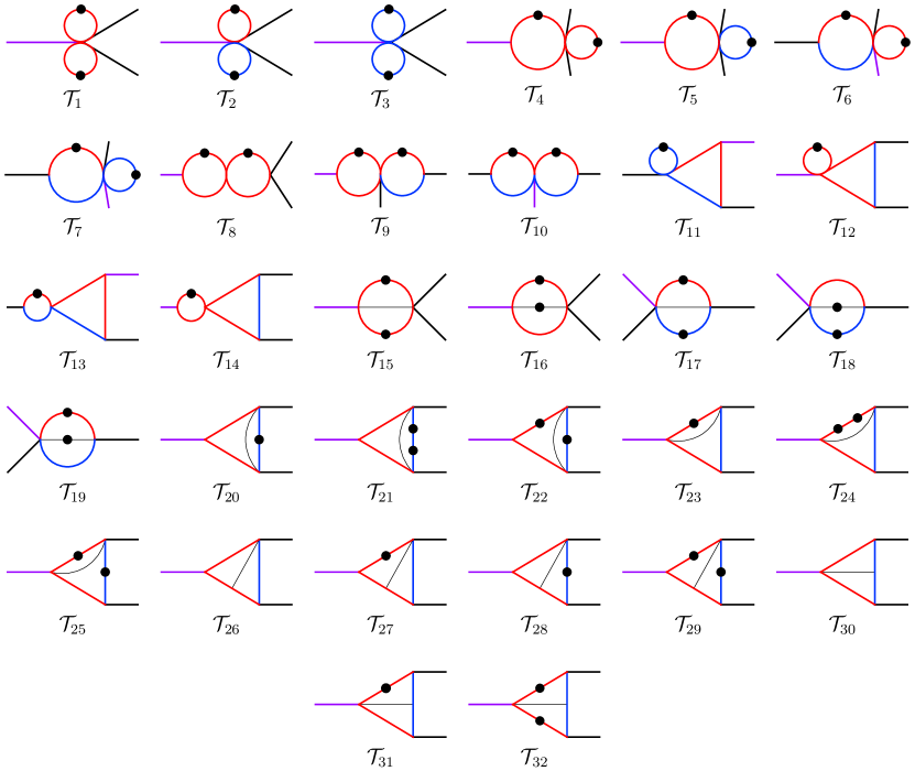
Figure 4: A set of pre-canonical basis for the integral family $\mathcal{F}$. The same signature as adopted in figure 2. Each black dot on an internal line represents an increase in the power of the corresponding propagator by one.

Following the algorithm suggested in refs. DiVita:2014pza , we employ the Magnus exponential method to establish a set of canonical MIs, which adheres to the system defined in eq. (25),

$$\text{I}_{1}=\, \text{F}_{1}\,, \text{I}_{2}=\, \text{F}_{2}\,,$$

$$\text{I}_{3}=\, \text{F}_{3}\,, \text{I}_{4}=\, \lambda_{1}\,\text{F}_{4}\,,$$

$$\text{I}_{5}=\, \lambda_{1}\,\text{F}_{5}\,, \text{I}_{6}=\, \frac{\lambda_{3}}{2}\frac{\text{F}_{1}-\text{F}_{2}-2m_{\scriptscriptstyle W}^{2}\text{F}_{6}}{m_{t}^{2}-m_{b}^{2}-m_{\scriptscriptstyle W}^{2}}\,,$$

$$\text{I}_{7}=\, \frac{\lambda_{3}}{2}\frac{\text{F}_{2}-\text{F}_{3}-2m_{\scriptscriptstyle W}^{2}\text{F}_{7}}{m_{t}^{2}-m_{b}^{2}-m_{\scriptscriptstyle W}^{2}}\,, \text{I}_{8}=\, \lambda_{1}^{2}\,\text{F}_{8}\,,$$

$$\text{I}_{9}=\, \frac{\lambda_{1}\lambda_{3}}{2}\frac{\text{F}_{4}-\text{F}_{5}-2m_{\scriptscriptstyle W}^{2}\text{F}_{9}}{m_{t}^{2}-m_{b}^{2}-m_{\scriptscriptstyle W}^{2}}\,,$$

$$\text{I}_{10}=\, \frac{-\lambda_{3}^{2}}{m_{t}^{2}-m_{b}^{2}-m_{\scriptscriptstyle W}^{2}}(\frac{1}{4}\,\text{F}_{1}-\frac{1}{2}\,\text{F}_{2}+\frac{1}{4}\,\text{F}_{3}-m_{\scriptscriptstyle W}^{2}\text{F}_{6}+m_{\scriptscriptstyle W}^{2}\text{F}_{7}+m_{\scriptscriptstyle W}^{4}\text{F}_{10})\,,$$

$$\text{I}_{11}=\, \lambda_{2}\,\text{F}_{11}\,, \text{I}_{12}=\, \lambda_{2}\,\text{F}_{12}\,,$$

$$\text{I}_{13}=\, \frac{-\lambda_{2}\lambda_{3}}{2}\frac{\text{F}_{11}-\text{F}_{12}+2m_{\scriptscriptstyle W}^{2}\text{F}_{13}}{m_{t}^{2}-m_{b}^{2}-m_{\scriptscriptstyle W}^{2}}\,, \text{I}_{14}=\, \lambda_{1}\lambda_{2}\,\text{F}_{14}\,,$$

$$\text{I}_{15}=\, s\,\text{F}_{15}\,, \text{I}_{16}=\, \frac{\lambda_{1}}{2}(\text{F}_{15}+2\,\text{F}_{16})\,,$$

$$\text{I}_{17}=\, m_{\scriptscriptstyle W}^{2}\text{F}_{17}\,, \text{I}_{18}=\, \lambda_{3}(\text{F}_{17}+\text{F}_{18}+\text{F}_{19})\,,$$

$$\text{I}_{19}=\, \frac{2m_{t}^{2}-2m_{b}^{2}-m_{\scriptscriptstyle W}^{2}}{4}\,\text{F}_{17}+\frac{m_{t}^{2}-m_{b}^{2}-m_{\scriptscriptstyle W}^{2}}{2}\,\text{F}_{18}+\frac{m_{t}^{2}-m_{b}^{2}+m_{\scriptscriptstyle W}^{2}}{2}\,\text{F}_{19}\,,$$

$$\text{I}_{20}=\, \lambda_{2}\,\text{F}_{20}\,, \text{I}_{21}=\, \lambda_{2}m_{b}^{2}\,\text{F}_{21}\,,$$

$$\text{I}_{22}=\, \lambda_{1}\big{(}\frac{3}{2}\,\text{F}_{20}+m_{b}^{2}\,\text{F}_{21}+(m_{t}^{2}-m_{\scriptscriptstyle W}^{2})\,\text{F}_{22}\big{)}\,, \text{I}_{23}=\, \lambda_{2}\,\text{F}_{23}\,,$$

$$\text{I}_{24}=\, \lambda_{2}m_{t}^{2}\,\text{F}_{24}\,,$$

$$\text{I}_{25}=\, \frac{\lambda_{3}}{s(m_{t}^{2}+m_{b}^{2}-m_{\scriptscriptstyle W}^{2})-m_{t}^{2}(m_{t}^{2}-m_{b}^{2}+m_{\scriptscriptstyle W}^{2})}\Big{[}\frac{s-m_{t}^{2}}{4}(-\text{F}_{1}+\text{F}_{2}+3s\,\text{F}_{15})$$

$$-\hbox to0.0pt{$\displaystyle\frac{s(m_{t}^{2}-3m_{b}^{2}+7m_{\scriptscriptstyle W}^{2})-m_{t}^{2}(m_{t}^{2}-m_{b}^{2}+5m_{\scriptscriptstyle W}^{2})}{8}\,\text{F}_{17}$\hss}$$

$$-\hbox to0.0pt{$\displaystyle\frac{s(m_{t}^{2}-3m_{b}^{2}-m_{\scriptscriptstyle W}^{2})-m_{t}^{2}(m_{t}^{2}-m_{b}^{2}-3m_{\scriptscriptstyle W}^{2})}{8}\,\text{F}_{18}$\hss}$$

$$-\hbox to0.0pt{$\displaystyle\frac{s(m_{t}^{2}-3m_{b}^{2}+3m_{\scriptscriptstyle W}^{2})-m_{t}^{2}(m_{t}^{2}-m_{b}^{2}+m_{\scriptscriptstyle W}^{2})}{8}\,\text{F}_{19}$\hss}$$

$$+\hbox to0.0pt{$\displaystyle\frac{3}{2}s(s-m_{t}^{2}+2m_{b}^{2}-2m_{\scriptscriptstyle W}^{2})\,\text{F}_{23}+sm_{t}^{2}(s-m_{t}^{2}+2m_{b}^{2}-2m_{\scriptscriptstyle W}^{2})\,\text{F}_{24}$\hss}$$

$$+\hbox to0.0pt{$\displaystyle\big{(}s^{2}m_{b}^{2}-sm_{t}^{2}(m_{b}^{2}+m_{\scriptscriptstyle W}^{2})+s(m_{b}^{2}-m_{\scriptscriptstyle W}^{2})^{2}+m_{t}^{4}m_{\scriptscriptstyle W}^{2}\big{)}\,\text{F}_{25}\Big{]}\,,$\hss}$$

$$\text{I}_{26}=\, \lambda_{2}\,\text{F}_{26}\,, \text{I}_{27}=\, \lambda_{1}\lambda_{2}\,\text{F}_{27}\,,$$

$$\text{I}_{28}=\, \lambda_{2}\lambda_{3}\,\text{F}_{28}\,,$$

$$\text{I}_{29}=\, s\frac{m_{t}^{2}+m_{b}^{2}-m_{\scriptscriptstyle W}^{2}}{m_{t}^{2}-m_{b}^{2}-m_{\scriptscriptstyle W}^{2}}(\text{F}_{4}-\text{F}_{5}-2m_{\scriptscriptstyle W}^{2}\text{F}_{9}\big{)}+s(s-2m_{t}^{2}+2m_{b}^{2}-2m_{\scriptscriptstyle W}^{2})\,\text{F}_{27}$$

$$+\hbox to0.0pt{$\displaystyle s(m_{t}^{2}-m_{b}^{2}-m_{\scriptscriptstyle W}^{2})\,\text{F}_{28}+s\big{(}(m_{t}^{2}-m_{\scriptscriptstyle W}^{2})^{2}+m_{b}^{2}(s-2m_{t}^{2}-2m_{\scriptscriptstyle W}^{2})+m_{b}^{4}\big{)}\,\text{F}_{29}\,,$\hss}$$

$$\text{I}_{30}=\, \lambda_{2}\,\text{F}_{30}\,, \text{I}_{31}=\, \lambda_{2}\lambda_{3}\,\text{F}_{31}\,,$$

$$\text{I}_{32}=\, \frac{sm_{b}^{2}}{(m_{t}^{2}-m_{b}^{2}-m_{\scriptscriptstyle W}^{2})^{2}}(-\text{F}_{1}+2\,\text{F}_{2}-\text{F}_{3}+4m_{\scriptscriptstyle W}^{2}\text{F}_{6}-4m_{\scriptscriptstyle W}^{2}\text{F}_{7}-4m_{\scriptscriptstyle W}^{4}\text{F}_{10})$$

$$+\hbox to0.0pt{$\displaystyle 2s(m_{t}^{2}-m_{b}^{2}-m_{\scriptscriptstyle W}^{2})\,\text{F}_{31}+s\big{(}(m_{t}^{2}-m_{\scriptscriptstyle W}^{2})^{2}+m_{b}^{2}(s-2m_{t}^{2}-2m_{\scriptscriptstyle W}^{2})+m_{b}^{4}\big{)}\,\text{F}_{32}\,,$\hss}$$

where $\lambda_{1,2,3}$ are three square roots related to the external kinematics as

$$\lambda_{1}^{2}=s(s-4m_{t}^{2})\,,\qquad\lambda_{2}^{2}=s(s-4m_{\scriptscriptstyle W}^{2})\,,\qquad\lambda_{3}^{2}=(m_{t}^{2}+m_{b}^{2}-m_{\scriptscriptstyle W}^{2})^{2}-4\,m_{t}^{2}\,m_{b}^{2}\,.$$ (34)

It is worth noting, all canonical MIs defined in eq. (LABEL:eq:UT_basis) are normalized to be finite in $\epsilon\to 0$. A further dimensional analysis reveals that all of these canonical MIs are dimensionless. To facilitate our subsequent discussions, we introduce the following three dimensionless variables:

$$\tau_{1}=-\frac{s}{m_{t}^{2}}\,,\qquad\tau_{2}=-\frac{m_{\scriptscriptstyle W}^{2}}{m_{t}^{2}}\,,\qquad\tau_{3}=\frac{m_{b}^{2}}{m_{t}^{2}}\,.$$ (35)

Then, we are able to derive the canonical differential equations of $\mathbf{I}$ with respect to $\tau_{1},\tau_{2}$ and $\tau_{3}$,

$$d\mathbf{I}(\tau_{1},\tau_{2},\tau_{3},\epsilon)=\epsilon\,d\mathbb{A}(\tau_{1},\tau_{2},\tau_{3})\,\mathbf{I}(\tau_{1},\tau_{2},\tau_{3},\epsilon)$$ (36)

with $d\mathbb{A}(\tau_{1},\tau_{2},\tau_{3})$ containing the following square roots:

$$\lambda_{1}^{\prime\,2}=\tau_{1}(\tau_{1}+4)\,,\qquad\lambda_{2}^{\prime\,2}=\tau_{1}(\tau_{1}-4\,\tau_{2})\,,\qquad\lambda_{3}^{\prime\,2}=(1+\tau_{2}+\tau_{3})^{2}-4\,\tau_{3}\,.$$ (37)

Furthermore, we introduce the following change of variables to eliminate these square roots,

$$\tau_{1}=\frac{(1-x)^{2}}{x}\,,\quad\tau_{2}=\frac{(1-x)^{2}z}{x(1+z)^{2}}\,,\quad\tau_{3}=\Big{(}1+\frac{y}{1+z}\Big{)}\Big{(}1-\frac{(1-x)^{2}z}{xy(1+z)}\Big{)}\,.$$ (38)

This transformation proves advantageous, as it enables the simultaneous rationalization of all three square roots, resulting in the conversion of them into a rational format,

$$\lambda_{1}^{\prime}=\frac{(1-x)(1+x)}{x}\,,\quad\lambda_{2}^{\prime}=\frac{(1-x)^{2}(1-z)}{x(1+z)}\,,\quad\lambda_{3}^{\prime}=\frac{(1-x)^{2}z+xy^{2}}{xy(1+z)}\,.$$ (39)

Consequently, the canonical differential equations satisfied by $\mathbf{I}$ with respect to $x,\,y$ and $z$ can be cast into the following dlog-form,

$$d\mathbf{I}(x,y,z,\epsilon)=\epsilon\,d\mathbb{A}(x,y,z)\,\mathbf{I}(x,y,z,\epsilon)=\epsilon\,\Big{(}\sum_{i=1}^{20}\mathbb{M}_{i}\operatorname{\mathit{d}log}\eta_{i}(x,y,z)\Big{)}\,\mathbf{I}(x,y,z,\epsilon)\,$$ (40)

with the 20 rational symbol letters read as

$$\eta_{1} =x\,, \eta_{2} =y\,,$$

$$\eta_{3} =z\,, \eta_{4} =1-x\,,$$

$$\eta_{5} =1+x\,, \eta_{6} =1+y\,,$$

$$\eta_{7} =1-z\,, \eta_{8} =1+z\,,$$

$$\eta_{9} =x+z\,, \eta_{10} =y+z\,,$$

$$\eta_{11} =1+xz\,, \eta_{12} =1-x+y\,,$$

$$\eta_{13} =-1+x+xy\,, \eta_{14} =1+y+z\,,$$

$$\eta_{15} =y+(1-x)z\,, \eta_{16} =xy-(1-x)z\,,$$

$$\eta_{17} =xy-(1-x)^{2}\,, \eta_{18} =xy-(1-x)^{2}z\,,$$

$$\eta_{19} =xy^{2}+(1-x)^{2}z\,, \eta_{20} =xy(1+z)-(1-x)^{2}z\,.$$ (41)

It is quite evident that all symbol letters are positive in the region

$$0<x<1\,,\qquad 0<z<1\,,\qquad y>\frac{1}{x}\,,$$ (42)

and all MIs are real functions of the dimensionless kinematic variables $x,\,y,$ and $z$.

As a direct consequence of the rational symbol letters, the integrations can be straightforwardly represented in terms of GPLs with arguments depending on the dimensionless variables $x,\,y,$ and $z$. The explicit expressions of coefficient matrices $\mathbb{M}_{i}$’s ($i=1,\dots,20$) defined in eq. (27) are collected in appendix A. The coefficient matrices $\mathbb{M}_{i}$’s are also provided in the ancillary files “dlog-form_Matrix.m” accompanying the arXiv version of this publication.

3.3 Boundary conditions

The canonical system of first-order differential equations (25) can be determined up to the integration constants. Therefore, the primary challenge here is to determine the integration constants, which effectively serve as the boundary conditions to fix the solutions uniquely. Unfortunately, there is not a mature automatic algorithm or available tools for this task. However, there are two commonly employed strategies for determining the boundary constants. On one hand, in principle, we can directly evaluate the integration constants by an independent, and often simpler, calculation at a preferred kinematic point, that can be characterized by accidental kinematic symmetries or specific kinematic limits or particular physical significances. In practice, this strategy frequently results in a significant reduction in the number of MIs, predigesting the task as we only need to concentrate on the evaluation the remaining independent MIs at that special point. Subsequently, in order to evaluate these reduced MIs at that point, we can explore various available analytical or numerical methods, such as Feynman parametrization with Cheng-Wu theorem Cheng:1987ga , Mellin-Barnes Smirnov:1999gc ; Tausk:1999vh , expansion by regions Beneke:1997zp , sector decomposition Heinrich:2008si ; Borowka:2017idc ; Smirnov:2021rhf and auxiliary mass flow Liu:2017jxz ; Liu:2022mfb ; Liu:2022chg . On the other hand, the integration constants can be determined by adhering the Ansatz equations in accordance with the behaviour of MIs around the singularities of the differential equations. The most common approach is stipulating the regularity of integrations at the spurious singularities, which are not singularities of integrals. By imposing regularity conditions, we are able to systematically establish a set of linear equations with undetermined constants of distinct integrals.

In our specific problem, we determine the integration constants by imposing the regularity of the canonical basis for vanishing external momenta, $s=m_{\scriptscriptstyle W}^{2}=0$. At this point, we find that the prefactors, as defined in eq. (LABEL:eq:UT_basis) for the canonical MIs become zero, with the exception of $\text{I}_{1,2,3,6,7,10,18,19,25}$. Furthermore, we notice that after setting $m_{b}=m_{t}$, the prefactors of $\text{I}_{18,19}$ also vanish. The remaining MIs can be expressed as the product of two one-loop massive tadpoles with mass $m_{t}$. Consequently, $\text{I}_{6,7,10,25}$ also vanish, due to the cancellation of tadpoles. Therefore, we only need to evaluate the remaining MIs, namely, $\text{I}_{1,2,3}$, which can be directly calculated by Feynman parametrization. With the integration measure normalized according to eq. (21), these MIs are all equal to one. Additionally, all the MIs illustrated in figure 4 are regular under these aforementioned conditions. Therefore, the integration constants of the canonical basis $\mathbf{I}$ can be determined at the special kinematic point, $s=m_{\scriptscriptstyle W}^{2}=0$ and $m_{b}=m_{t}$, corresponding to a base-point $\vec{x}_{0}=(x_{0},y_{0},z_{0})=(1,0,0)$,

$$\text{I}_{i}(\vec{x}_{0},\epsilon)=\begin{cases}\;1,\qquad&i=1,2,3,\\ \;0,\qquad&i\neq 1,2,3.\end{cases}$$ (43)

All MIs are presented in terms of GPLs, whose weights of arguments $x,\,y,$ and $z$ are listed in table 1. The evaluation of our analytical results relies on the Mathematica package PolyLogTools Maitre:2005uu ; Maitre:2007kp ; Duhr:2019tlz and the C++ library GiNaC Bauer:2000cp ; Vollinga:2004sn for the numerical evaluation of GPLs. To ensure the accuracy and reliability of our results, all master integrals have been numerically cross checked through the use of the publicly available packages pySecDec and AMFlow. This verification was conducted with high precision, in both the Euclidean and the physical regions. We have further provided the explicit expressions of all MIs, denoted as $\text{I}_{1,\dots,32}$ up to $\mathcal{O}(\epsilon^{2})$ in appendix A. The comprehensive analytic expressions up to weight four of all MIs are available in the supplementary file “analytic_MIs.m”, accompanying the arXiv submission of this paper.

argument	weight
$x$	$\big{\{}-1,\,0,\,1\,\big{\}}$
$y$	$\big{\{}-1,\,0,\,x-1,\,(1-x)/x,\,(1-x)^{2}/x\,\big{\}}$
$z$	$\big{\{}-1,\,0,\,1,\,-x,\,-1/x,\,-y,\,-1-y,\,-y/(1-x),$
	$xy/(1-x),\,xy/(1-x)^{2},\,-xy^{2}/(1-x)^{2},\,xy/((1-x)^{2}-xy)\,\big{\}}$

Table 1: The weights of GPLs, for arguments $x,\,y,$ and $z$.

3.4 Analytic continuation

At this point, we have successfully derived the explicit analytic expressions for the canonical MIs in the Euclidean regions as specified by eq. (42). Therefore, the remaining task is to elaborate on the prescriptions for the analytic continuation to arbitrary values of $x,\,y,$ and $z$. Some discussions on analytic continuation to the physical region can be found in refs. Birthwright:2004kk ; Gehrmann:2013cxs ; Bonciani:2016ypc ; DiVita:2017xlr . However, it is essential to acknowledge that the previous discussions cannot directly apply to the kinematic variables defined in eqs. $(\ref{eq:tauVars}\mbox{-}\ref{eq:rationalize})$. Thus, we need to delve into the specifics of the analytic continuation for the kinematics $x,\,y,$ and $z$. To delineate the permissible range of values for variables $x,\,y,$ and $z$, we must inverse the transformation in eqs. (35) and (38). Region by region in the kinematic variables space, we can assign the correct values to $x,\,y,$ and $z$, and ascertain the proper sign of the vanishing imaginary part (if present) arising from the Feynman prescription

$$s+i0^{+}\,,\qquad m_{\scriptscriptstyle W}^{2}+i0^{+}\,.$$ (44)

All of this can be accomplished while keeping the values of $m_{t}^{2}$ and $m_{b}^{2}$ remain positive.

3.4.1 Analytic continuation for $x$

Without loss of generality, let us consider the variable $x$ as defined by eqs. (35) and (38) and apply the following inverse transformation,

$$x=\frac{\sqrt{4\,m_{t}^{2}-s}-\sqrt{-s}}{\sqrt{4\,m_{t}^{2}-s}+\sqrt{-s}}\,.$$ (45)

It is imperative to carefully evaluate $x$ when $s>0$, as the inverse transformation in eq. (45) involves the square root of $s$ and $m_{t}^{2}$. Keeping $m_{t}^{2}>0$, we observe the following variations of $x$ with respect to $s$:

1. When $s<0$, all square roots appearing in eq. (45) yield real values, resulting in a real $x$ within the range of $0<x<1$.

2. When $0<s<4m_{t}^{2}$, $x$ assumes a pure phase

   $$x=e^{i\phi}$$ (46)

   with $\phi=2\arctan\sqrt{\frac{s}{4m_{t}^{2}-s}}$ and $0<\phi<\pi$.

3. When $s>4m_{t}^{2}$, $x$ takes on a negative value, while retaining a positive, diminishing imaginary part,

   $$x=-x^{\prime}+i0^{+}\,,\qquad 0<x^{\prime}<1\,.$$ (47)

3.4.2 Analytic continuation for $z$

Evidently, the variable $\tau_{2}$ depends on both $x$ and $z$. In order to disentangle the dependences on $x$ and $z$, we introduce the ratio $R$ as

$$R\equiv\frac{\tau_{1}}{\tau_{2}}=\frac{s}{m_{\scriptscriptstyle W}^{2}}\,.$$ (48)

This ratio, $R$, solely depends on the variable $z$:

$$R=\frac{(1+z)^{2}}{z}\,.$$ (49)

To determine the permissible range of value for $z$, we employ the inverse transformation,

$$z=\frac{\sqrt{R}-\sqrt{R-4}}{\sqrt{R}+\sqrt{R-4}}\,.$$ (50)

Particular care is required when evaluating $z$ for the cases when $R<4$ and $R<0$, as the inverse transformation in eq. (50) contains the square roots of $R$ and $R-4$. Maintaining the stipulation of vanishing imaginary part, $R\pm i0^{+}$, we observe the following three distinct variations of $z$ with respect to $R\,$:

1. When $R>4$, all square roots appearing in eq. (50) yield real values, resulting in positive $z$ within the range of $0<z<1$.

2. When $0<R<4$, with the specific prescription $R\pm i0^{+}$, $z$ becomes a pure phase

   $$z=e^{\mp i\psi}$$ (51)

   with $\psi=2\arctan\sqrt{\frac{4-R}{R}}$ and $0<\psi<\pi$.

3. When $R<0$, while adhering to the prescription $R\pm i0^{+}$, $z$ becomes negative with a vanishing imaginary part,

   $$z=-z^{\prime}\mp i0^{+}\,,\qquad 0<z^{\prime}<1\,.$$ (52)

It is important to emphasize that the accurate determination of values for $z$ is contingent upon the prescription used for $R$. Consequently, it becomes crucial to monitor the behaviour of the vanishing imaginary parts of $s$ and $m_{\scriptscriptstyle W}^{2}$ to ascertain the correct sign of the vanishing imaginary part of $z$, should it be present, within various kinematic regions.

3.4.3 Analytic continuation for $y$

Lastly, the variable $\tau_{3}$ depends on all three kinematic variables $x,\,y,$ and $z$. In order to establish the range of values for $y$, it becomes essential to disentangle the dependence of $\tau_{3}$ on $y$ from that on $x$ and $z$. To facilitate subsequent discussions, we introduce two intermediate variables as

$$\sigma_{1}\equiv\frac{y}{1+z}\,,\qquad\sigma_{2}\equiv\frac{(1-x)^{2}z}{x(1+z)y}\,.$$ (53)

This allows us to represent $\tau_{2},\tau_{3}$ and $\lambda_{3}^{\prime}$ in terms of $\sigma_{1},\sigma_{2}$,

$$\tau_{2}=\sigma_{1}\sigma_{2}\,,\qquad\tau_{3}=(1+\sigma_{1})(1-\sigma_{2})\,,\qquad\lambda_{3}^{\prime}=\sigma_{1}+\sigma_{2}\,.$$ (54)

The definitions in eq. (53) imply the necessity to solve the transformation from $\tau_{2},\tau_{3}$ to $\sigma_{1},\sigma_{2}$ to determine the solution for $y$. Without loss of generality, we adopt the following transformation:

$$\sigma_{1} =\frac{1}{2}(\tau_{2}+\tau_{3}-1+\lambda_{3}^{\prime})\,,$$

$$\sigma_{2} =-\frac{1}{2}(\tau_{2}+\tau_{3}-1-\lambda_{3}^{\prime})\,.$$ (55)

Furthermore, the solution for $y$ is

$$y=(1+z)\sigma_{1}=\frac{1}{2}(1+z)(\tau_{2}+\tau_{3}-1+\lambda_{3}^{\prime}(\tau_{2},\tau_{3}))\,,$$ (56)

where the expression of $\lambda_{3}^{\prime}(\tau_{2},\tau_{3})$ can be found in eq. (37).

As established in our earlier discussion, we are aware of that $\tau_{3}$ is positive. Therefore, the vanishing imaginary part of $y$, if it exists, must comes from the contribution of $\tau_{2}$ and $z$. Our understanding of the analytic continuation for $z$ is well-informed by the detailed exposition in section 3.4.2. Now, the primary challenge lies in determining the domain for $\sigma_{1}$. Keeping the prescription of $R\pm i0^{+}$ and $\tau_{2}-i0^{+}$ for cases where $\tau_{2}<0$, we can delineate the following scenarios:

1. When $\tau_{2}>0$ and $\tau_{3}>0$, the third square root in eq. (37) is real. Consequently, $\lambda_{3}^{\prime}(\tau_{2},\tau_{3})>0$, and further, $\sigma_{1}>0$.

2. When $\tau_{2}<0$ and $\tau_{3}>1-\tau_{2}+2\sqrt{-\tau_{2}}$, $\sigma_{1}$ becomes positive while possessing a negative vanishing imaginary part,

   $$\sigma_{1}=\sigma_{1}^{\prime}-i0^{+}\,,\qquad\sigma_{1}^{\prime}>0\,.$$ (57)

3. When $-1<\tau_{2}<0$ and $0<\tau_{3}<1-\tau_{2}-2\sqrt{-\tau_{2}}$, $\sigma_{1}$ turns negative while maintaining a negative vanishing imaginary part,

   $$\sigma_{1}=\sigma_{1}^{\prime}-i0^{+}\,,\qquad\sigma_{1}^{\prime}<0\,.$$ (58)

4. When $\tau_{2}<-1$ and $0<\tau_{3}<1-\tau_{2}-2\sqrt{-\tau_{2}}$, $\sigma_{1}$ becomes negative with a positive vanishing imaginary part,

   $$\sigma_{1}=\sigma_{1}^{\prime}+i0^{+}\,,\qquad\sigma_{1}^{\prime}<0\,.$$ (59)

5. When $\tau_{2}<0$ and $1-\tau_{2}-2\sqrt{-\tau_{2}}<\tau_{3}<1-\tau_{2}-2\sqrt{-\tau_{2}}$, $\lambda_{3}^{\prime}(\tau_{2},\tau_{3})$ becomes complex, owing to its negative square root, with a non-vanishing imaginary part.

Incorporating the insights from our prior discussion on the analytic continuation variable $z$, we can derive the comprehensive analytic continuation for $y$ across the distinct regions of $R>4$, $0<R<4$ and $R<0$. Given the straightforward nature of the relationship between $z$ and $\sigma_{1}$, it is unnecessary to detail the analytic continuation for $y$ on a case-by-case basis.

To facilitate the calculations involved in the $e^{+}e^{-}\to W^{+}W^{-}$ process, we summarize the analytic continuation for $x$, $y$, and $z$ in various physical regions and present them in table 2. The solutions listed in the second and third rows pertain to the canonical MIs stemming from the integral family $\mathcal{F}$, as defined in eq. (23). For completeness, we also include the solution for the integral family $\mathcal{F}^{*}$ in the last row.

region	$x$	$z$	$y$
$4m_{\scriptscriptstyle W}^{2}<s<4m_{1}^{2}$	$e^{i\phi}$	$z$	$-y^{\prime}-i0^{+}$
$4m_{\scriptscriptstyle W}^{2}<4m_{1}^{2}<s$	$-x^{\prime}+i0^{+}$	$z$	$-y^{\prime}-i0^{+}$
$4m_{1}^{2}<4m_{\scriptscriptstyle W}^{2}<s$	$-x^{\prime}+i0^{+}$	$z$	$y^{\prime}-i0^{+}$

Table 2: Solutions for $x$, $y$, and $z$ in the physical region of the $s$-plane, as required by $e^{+}e^{-}\to W^{+}W^{-}$. In the second and third rows, $m_{1}=m_{t}$ and $m_{2}=m_{b}$, and both $s$-plane regions meet the criteria of $R>4\,,-1<\tau_{2}<0$, and $0<\tau_{3}<1-\tau_{2}-2\sqrt{-\tau_{2}}$. While in the last row, we denote $m_{1}=m_{b}$ and $m_{2}=m_{t}$, and the $s$-plane region adheres to the conditions $R>4\,,\tau_{2}<0$, and $\tau_{3}>1-\tau_{2}-2\sqrt{-\tau_{2}}$.

4 Numerical results and discussion

Leveraging the analytical results of all two-loop canonical MIs derived in section 3, we calculate the integrated cross section and some kinematic distributions of final-state $W$ boson for $e^{+}e^{-}\to W^{+}W^{-}$ up to the QCD-EW NNLO. All the leptons and light quarks ($u$, $d$, $c$ and $s$) are treated as massless particles. The relevant SM input parameters used in this paper are taken as ParticleDataGroup:2020ssz

$$m_{\scriptscriptstyle Z} =91.1876~{}\mathrm{GeV}\,, m_{t}=172.5~{}\mathrm{GeV}\,, \alpha(0)=1/137.035999084\,,$$

$$m_{\scriptscriptstyle W} =80.379~{}\mathrm{GeV}\,, m_{b}=4.78~{}\mathrm{GeV}\,, G_{\mu}=1.1663787\times 10^{-5}~{}\mathrm{GeV}^{-2}\,,$$

$$m_{\scriptscriptstyle H} =125.25~{}\mathrm{GeV}\,, \alpha_{s}(M_{Z})=0.1179\,.$$ (60)

We use the Mathematica package RunDec Chetyrkin:2000yt ; Schmidt:2012az ; Herren:2017osy to evaluate the strong coupling constant $\alpha_{s}(\mu)$ at $\mu=m_{\scriptscriptstyle W}$, and conduct the numerical calculation in both $\alpha(0)$ and $G_{\mu}$ schemes, wherein the fine structure constant $\alpha$ is taken as $\alpha(0)$ and $\alpha_{\scriptscriptstyle G_{\mu}}$ as defined in eqs. (60) and (12), respectively.

4.1 Integrated cross sections

Up to the QCD-EW NNLO, the integrated cross section for $e^{+}e^{-}\to W^{+}W^{-}$ can be formulated as

$$\sigma_{\scriptscriptstyle\mathrm{NNLO}} =\sigma_{\scriptscriptstyle\mathrm{LO}}(1+\delta_{\scriptscriptstyle\mathrm{EW}}+\delta_{\scriptscriptstyle\mathrm{QCD\mbox{-}EW}})\,,$$ (61)

where $\delta_{\scriptscriptstyle\mathrm{EW}}$ and $\delta_{\scriptscriptstyle\mathrm{QCD\mbox{-}EW}}$ represent the NLO EW and NNLO mixed QCD-EW corrections normalized by LO cross section

$$\delta_{\scriptscriptstyle\mathrm{EW}}=\frac{\Delta\sigma_{\scriptscriptstyle\mathrm{EW}}}{\sigma_{\scriptscriptstyle\mathrm{LO}}}\,,\qquad\delta_{\scriptscriptstyle\mathrm{QCD\mbox{-}EW}}=\frac{\Delta\sigma_{\scriptscriptstyle\mathrm{QCD\mbox{-}EW}}}{\sigma_{\scriptscriptstyle\mathrm{LO}}}\,.$$ (62)

In figure 5, we illustrate the LO and NNLO corrected integrated cross sections as functions of the $e^{+}e^{-}$ colliding energy, $\sqrt{s}$, for the process $e^{+}e^{-}\to W^{+}W^{-}$ in both $\alpha(0)$ (left) and $G_{\mu}$ (right) schemes. The corresponding EW and QCD-EW relative corrections are visualized in the lower panels. As shown in this figure, the production cross sections exhibit consistent behaviours across different schemes. The cross sections skyrocket near the $W$-pair production threshold, and reach their maxima at $\sqrt{s}\sim 195\,\mathrm{GeV}$, followed by a smooth decrease as the increase of $\sqrt{s}$ in the high-energy region. The emergence of this peak can be explained by the competition between the enlargement of phase-space and the s-channel suppression as the increase of $\sqrt{s}$. As depicted in the lower panels, the EW corrections lead to a significant suppression of LO cross section in the vicinity of the threshold, reaching about $-30\%$, and gradually transition to a moderate enhancement in the high-energy region, exceeding approximately $5\%$ and $9\%$ at $\sqrt{s}=1000\,\mathrm{GeV}$ in the $\alpha(0)$ and $G_{\mu}$ schemes, respectively. The substantial EW relative corrections near the threshold are attributed to the Coulomb singularity effect Denner:1991kt ; Beenakker:1996kt . The virtual EW corrections are enhanced by Coulombic photon exchange between the electron and positron in Feynman loops when the photon momentum approaches zero. The mixed QCD-EW corrections result in a slight enhancement of the production cross section across the entire plotted energy region, amounting to approximately $0.9\%$ in the $\alpha(0)$ scheme. However, the magnitude of the mixed QCD-EW relative correction is considerably reduced in the $G_{\mu}$ scheme. It can be attributed to the fact that some significant universal higher-order corrections are absorbed into the LO cross section Denner:1991kt ; Beenakker:1996kt ; Denner:2019vbn . The mixed QCD-EW relative correction peaks at $\sqrt{s}=2m_{t}$, which can be interpreted as the resonance effect induced by the top-quark loop integrals. In the $\alpha(0)$ and $G_{\mu}$ schemes, the QCD-EW relative corrections reach about $9.4\text{\textperthousand}$ and $0.4\text{\textperthousand}$, respectively, at the resonance peak. The LO, NLO EW and NNLO mixed QCD-EW corrected integrated cross sections along with the corresponding relative corrections at some representative colliding energies for both $\alpha(0)$ and $G_{\mu}$ schemes are listed in table 3. Considering the more significant magnitude of mixed QCD-EW corrections in the $\alpha(0)$ scheme, in the subsequent discussion, we concentrate on the phenomenological analysis in the $\alpha(0)$ scheme.

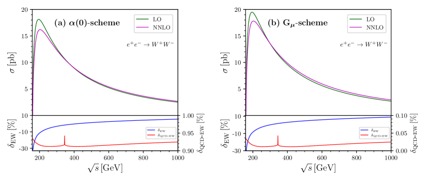
Figure 5: LO and NNLO corrected integrated cross sections, along with the corresponding EW and QCD-EW relative corrections for $e^{+}e^{-}\to W^{+}W^{-}$ as functions of colliding energy.

$\sqrt{s}$ [GeV]	schemes	$\sigma_{\scriptscriptstyle\mathrm{LO}}[\mathrm{pb}]$	$\sigma_{\scriptscriptstyle\mathrm{NLO}}[\mathrm{pb}]$	$\delta_{\scriptscriptstyle\mathrm{EW}}[\%]$	$\sigma_{\scriptscriptstyle\mathrm{NNLO}}[\mathrm{pb}]$	$\delta_{\scriptscriptstyle\mathrm{QCD\mbox{-}EW}}[\%]$
$161$	$\alpha(0)$	$~{}2.766743$	$~{}1.91742$	$-30.6975$	$~{}1.94325$	$0.9336$
	$G_{\mu}$	$~{}2.973577$	$~{}2.11078$	$-29.0156$	$~{}2.11179$	$0.0339$
$200$	$\alpha(0)$	$18.075506$	$16.01245$	$-11.4136$	$16.17810$	$0.9164$
	$G_{\mu}$	$19.426781$	$17.79225$	$\;\,-8.4138$	$17.79535$	$0.0160$
$240$	$\alpha(0)$	$15.961183$	$14.90107$	$\;\,-6.6418$	$15.04671$	$0.9124$
	$G_{\mu}$	$17.154397$	$16.56135$	$\;\,-3.4571$	$16.56337$	$0.0118$
$250$	$\alpha(0)$	$15.342627$	$14.44029$	$\;\,-5.8813$	$14.58025$	$0.9122$
	$G_{\mu}$	$16.489600$	$16.04952$	$\;\,-2.6688$	$16.05143$	$0.0116$
$350$	$\alpha(0)$	$10.514905$	$10.34951$	$\;\,-1.5730$	$10.44576$	$0.9155$
	$G_{\mu}$	$11.300970$	$11.50336$	$~{}~{}\;\,1.7909$	$11.50504$	$0.0149$
$500$	$\alpha(0)$	$~{}6.684693$	$~{}6.76970$	$~{}~{}\;\,1.2717$	$~{}6.83075$	$0.9133$
	$G_{\mu}$	$~{}7.184422$	$~{}7.52419$	$~{}~{}\;\,4.7293$	$~{}7.52511$	$0.0127$
$1000$	$\alpha(0)$	$~{}2.497517$	$~{}2.63439$	$~{}~{}\;\,5.4806$	$~{}2.65749$	$0.9249$
	$G_{\mu}$	$~{}2.684224$	$~{}2.92760$	$~{}~{}\;\,9.0667$	$~{}2.92826$	$0.0247$

Table 3: LO, NLO EW and NNLO QCD-EW corrected integrated cross sections, as well as the corresponding EW and QCD-EW relative corrections for $e^{+}e^{-}\to W^{+}W^{-}$.

4.2 Kinematic distributions

In this subsection, we study some kinematic distributions of the final-state $W$ boson for $e^{+}e^{-}\to W^{+}W^{-}$. The EW and QCD-EW differential relative corrections with respect to the kinematic variable $x$ are defined as

$$\delta_{\scriptscriptstyle\mathrm{EW}}=\Big{(}\frac{\mathrm{d}\sigma_{\scriptscriptstyle\mathrm{EW}}}{\mathrm{d}x}-\frac{\mathrm{d}\sigma_{\scriptscriptstyle\mathrm{LO}}}{\mathrm{d}x}\Big{)}/\frac{\mathrm{d}\sigma_{\scriptscriptstyle\mathrm{LO}}}{\mathrm{d}x},\qquad\delta_{\scriptscriptstyle\mathrm{QCD\mbox{-}EW}}=\Big{(}\frac{\mathrm{d}\sigma_{\scriptscriptstyle\mathrm{QCD\mbox{-}EW}}}{\mathrm{d}x}-\frac{\mathrm{d}\sigma_{\scriptscriptstyle\mathrm{LO}}}{\mathrm{d}x}\Big{)}/\frac{\mathrm{d}\sigma_{\scriptscriptstyle\mathrm{LO}}}{\mathrm{d}x}.$$ (63)

As a consequence of the CP conservation, we have the following symmetry relations for the differential distributions of $W^{+}$ and $W^{-}$,

$$\frac{\mathrm{d}\sigma}{\mathrm{d}\cos\theta_{\scriptscriptstyle W^{-}}}=\frac{\mathrm{d}\sigma}{\mathrm{d}\cos\theta_{\scriptscriptstyle W^{+}}}\Big{|}_{\theta_{\scriptscriptstyle W^{+}}\to\pi-\theta_{\scriptscriptstyle W^{-}}}\,,\qquad\frac{\mathrm{d}\sigma}{\mathrm{d}p_{T}^{\scriptscriptstyle W^{-}}}=\frac{\mathrm{d}\sigma}{\mathrm{d}p_{T}^{\scriptscriptstyle W^{+}}}\Big{|}_{p_{T}^{\scriptscriptstyle W^{+}}\to p_{T}^{\scriptscriptstyle W^{-}}}\,.\qquad$$ (64)

Thus, the transverse momentum distribution of $W^{-}$ is identical to that of $W^{+}$, and the scattering angle distribution of $W^{-}$ can be obtained by reversing the scattering angle distribution of $W^{+}$. Consequently, we restrict our focus to the differential distributions of $W^{+}$ in the subsequent discussion, and denote ${\mathrm{d}\sigma}/{\mathrm{d}\cos\theta}$ and ${\mathrm{d}\sigma}/{\mathrm{d}p_{T}}$ as the scattering angle and transverse momentum distributions of $W^{+}$, respectively.

In figure 6, we demonstrate the LO and NNLO corrected scattering angle distributions of the final-state $W^{+}$ boson, along with the corresponding EW and QCD-EW relative corrections for $e^{+}e^{-}\to W^{+}W^{-}$ at $\sqrt{s}=200$ and $500\,\mathrm{GeV}$. The scattering angle distribution strongly peaks in the forward direction, particularly at high energies, and decreases consistently as the increase of the scattering angle. As illustrated in the left plot of figure 6, the EW correction exhibits a moderate enhancement of approximately $10\%$ to the LO differential cross section in the backward direction, and transitions into a suppression of around $-20\%$ in the forward direction, at $\sqrt{s}=200\,\mathrm{GeV}$. The boost effect on the scattering angle distribution in the backward direction can be observed from the EW relative correction. Hard photon radiations boost the CM system of the $W$-pair, resulting in a migration of contributions in the forward region to the backward region, and vice versa. Since the cross section in the forward direction is substantially larger than that in the backward direction, the net effect of the redistribution of contributions from different regions leads to a distortion of the scattering angle distribution with respect to the LO distribution. The boost effect is significantly more prominent at high energies, as is evident from the comparison of the EW relative corrections at $\sqrt{s}=200$ and $500~{}\mathrm{GeV}$ plotted in the two lower panels of figure 6. In particular, the NLO EW correction in the extreme backward direction can be a dozen times greater than the LO cross section, which heavily destroys the reliability of perturbation calculation in this region. In contrast to the NLO EW corrections, there is no boost effect on the NNLO mixed QCD-EW corrections to $e^{+}e^{-}\to W^{+}W^{-}$, due to the absence of photon and gluon emissions. The NNLO QCD-EW corrections slightly enhance the LO scattering angle distribution in the whole $\cos\theta$ region. The QCD-EW relative correction is more sensitive to $\cos\theta$ in the backward region compared to the forward region. It increases monotonically as the increase of $\cos\theta$. At $\sqrt{s}=200~{}\mathrm{GeV}$, the QCD-EW relative correction increases from approximately $0.7\%$ to about $1\%$ with the increment of $\cos\theta$ from $-1$ to $1$. While at $\sqrt{s}=500~{}\mathrm{GeV}$, it varies from around $0\%$ to about $0.9\%$ as $\cos\theta$ increases from $-1$ to $0.4$, and becomes steady at $0.9\%$ in the range of $\cos\theta\in[0.4,1]$.

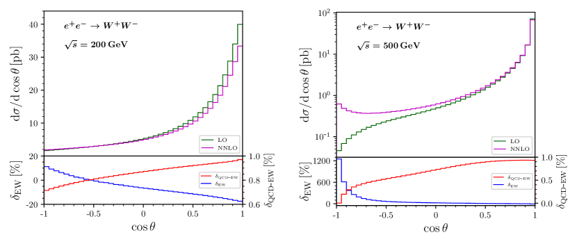
Figure 6: LO, NNLO corrected scattering angle distributions of the final-state $W^{+}$ boson, along with the corresponding EW and QCD-EW relative corrections for $e^{+}e^{-}\to W^{+}W^{-}$, at $\sqrt{s}=200$ (left) and $500~{}\mathrm{GeV}$ (right).

The LO and NNLO corrected transverse momentum distributions of the final-state $W^{+}$ boson, along with the corresponding EW and QCD-EW relative corrections, are plotted in figure 7. As can be seen from this figure, the $W$-boson pairs are mostly produced in the high $p_{T}$ region at $\sqrt{s}=200~{}\mathrm{GeV}$, while the events are mostly concentrated in the low $p_{T}$ region at $\sqrt{s}=500~{}\mathrm{GeV}$. The NLO EW correction enhances the LO differential cross section in the low $p_{T}$ region while suppresses the LO distribution in the high $p_{T}$ region. The Sudakov effect is responsible for the pronounced magnitude of the EW relative correction in the high $p_{T}$ region. The QCD-EW relative correction is more sensitive to the transverse momentum as the increase of the $e^{+}e^{-}$ colliding energy, especially in the high $p_{T}$ region. At $\sqrt{s}=500~{}\mathrm{GeV}$, the QCD-EW relative correction is steady at around $0.9\%$ in the range of $p_{T}<150~{}\mathrm{GeV}$, and decreases to about $0.75\%$. Combining the transverse momentum and the scattering angle distributions, we can conclude that the mixed QCD-EW correction exceeds $0.7\%$ in most of the phase-space regions and can reach about $1\%$. Therefore, the NNLO mixed QCD-EW corrections have non-negligible implications for future comparison with the high-precision experimental data, especially in some specific phase-space region.

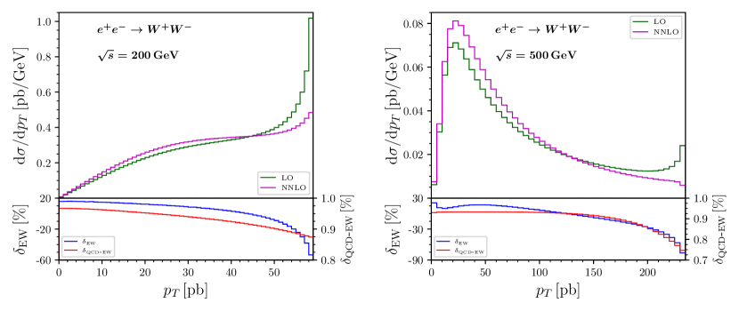
Figure 7: The same as figure 6, but for the transverse momentum distributions of the final-state $W^{+}$ boson.

5 Summary

The discrepancy between the CDF measurement and the SM theoretical prediction for the $W$-boson mass underscores the importance of the refinement on both theoretical predictions and experimental measurements. In this paper, we present a comprehensive calculation of the NNLO mixed QCD-EW corrections to the $W$-pair production at electron-positron colliders. Utilizing the canonical differential equation method, we perform an analytic calculation of all the two-loop MIs involved in the NNLO QCD-EW corrections, and obtain the 32 canonical MIs for TGC vertices, expressed in terms of GPLs up to the order of $\epsilon^{4}$. Leveraging the analytic expressions of these two-loop canonical MIs, we calculate the total production cross section and the differential distributions with respect to the scattering angle and transverse momentum of the final-state $W$ bosons in both $\alpha(0)$ and $G_{\mu}$ schemes. We find that the NNLO mixed QCD-EW corrections enhance the LO cross section. In the $\alpha(0)$ scheme, the relative correction exceeds $0.7\%$ in most of the phase-space regions, and can even reach about $1\%$ in some specific phase-space region. These NNLO mixed QCD-EW corrections have non-negligible implications for future comparison with the high-precision experimental data. Compared to the $\alpha(0)$ scheme, the NNLO QCD-EW correction in the $G_{\mu}$ scheme is relatively small. To reduce the dependence of the theoretical predictions on the input scheme of $\alpha$, it is imperative to take into account the NNLO pure EW $\mathcal{O}(\alpha^{2})$ corrections, which beyond the scope of this paper and will be investigated in the future.

Appendix A Coefficient matrices

In this appendix, we present the explicit expressions of the 20 coefficient matrices $\mathbb{M}_{i}$ ($i=1,\dots,20$) appearing in the $\operatorname{\mathit{d}log}$-form eq. (40).

$$\mathbb{M}_{1}= \left(\,\setcounter{MaxMatrixCols}{33}\begin{matrix}\hphantom{\scalebox{0.5}[1.0]{$-$}}0&\hphantom{\scalebox{0.5}[1.0]{$-$}}1&\hphantom{\scalebox{0.5}[1.0]{$-$}}0&\hphantom{\scalebox{0.5}[1.0]{$-$}}0&\hphantom{\scalebox{0.5}[1.0]{$-$}}0&\hphantom{\scalebox{0.5}[1.0]{$-$}}0&\hphantom{\scalebox{0.5}[1.0]{$-$}}0&\hphantom{\scalebox{0.5}[1.0]{$-$}}0&\hphantom{\scalebox{0.5}[1.0]{$-$}}0&\hphantom{\scalebox{0.5}[1.0]{$-$}}0&\hphantom{\scalebox{0.5}[1.0]{$-$}}0&\hphantom{\scalebox{0.5}[1.0]{$-$}}0&\hphantom{\scalebox{0.5}[1.0]{$-$}}0&\hphantom{\scalebox{0.5}[1.0]{$-$}}0&\hphantom{\scalebox{0.5}[1.0]{$-$}}0&\hphantom{\scalebox{0.5}[1.0]{$-$}}0&\hphantom{\scalebox{0.5}[1.0]{$-$}}0&\hphantom{\scalebox{0.5}[1.0]{$-$}}0&\hphantom{\scalebox{0.5}[1.0]{$-$}}0&\hphantom{\scalebox{0.5}[1.0]{$-$}}0&\hphantom{\scalebox{0.5}[1.0]{$-$}}0&\hphantom{\scalebox{0.5}[1.0]{$-$}}0&\hphantom{\scalebox{0.5}[1.0]{$-$}}0&\hphantom{\scalebox{0.5}[1.0]{$-$}}0&\hphantom{\scalebox{0.5}[1.0]{$-$}}0&\hphantom{\scalebox{0.5}[1.0]{$-$}}0&\hphantom{\scalebox{0.5}[1.0]{$-$}}0&\hphantom{\scalebox{0.5}[1.0]{$-$}}0&\hphantom{\scalebox{0.5}[1.0]{$-$}}0&\hphantom{\scalebox{0.5}[1.0]{$-$}}0&\hphantom{\scalebox{0.5}[1.0]{$-$}}0&\hphantom{\scalebox{0.5}[1.0]{$-$}}0&\hphantom{\scalebox{0.5}[1.0]{$-$}}0\\ \hphantom{\scalebox{0.5}[1.0]{$-$}}0&\hphantom{\scalebox{0.5}[1.0]{$-$}}0&\hphantom{\scalebox{0.5}[1.0]{$-$}}2&\hphantom{\scalebox{0.5}[1.0]{$-$}}0&\hphantom{\scalebox{0.5}[1.0]{$-$}}0&\hphantom{\scalebox{0.5}[1.0]{$-$}}0&\hphantom{\scalebox{0.5}[1.0]{$-$}}0&\hphantom{\scalebox{0.5}[1.0]{$-$}}0&\hphantom{\scalebox{0.5}[1.0]{$-$}}0&\hphantom{\scalebox{0.5}[1.0]{$-$}}0&\hphantom{\scalebox{0.5}[1.0]{$-$}}0&\hphantom{\scalebox{0.5}[1.0]{$-$}}0&\hphantom{\scalebox{0.5}[1.0]{$-$}}0&\hphantom{\scalebox{0.5}[1.0]{$-$}}0&\hphantom{\scalebox{0.5}[1.0]{$-$}}0&\hphantom{\scalebox{0.5}[1.0]{$-$}}0&\hphantom{\scalebox{0.5}[1.0]{$-$}}0&\hphantom{\scalebox{0.5}[1.0]{$-$}}0&\hphantom{\scalebox{0.5}[1.0]{$-$}}0&\hphantom{\scalebox{0.5}[1.0]{$-$}}0&\hphantom{\scalebox{0.5}[1.0]{$-$}}0&\hphantom{\scalebox{0.5}[1.0]{$-$}}0&\hphantom{\scalebox{0.5}[1.0]{$-$}}0&\hphantom{\scalebox{0.5}[1.0]{$-$}}0&\hphantom{\scalebox{0.5}[1.0]{$-$}}0&\hphantom{\scalebox{0.5}[1.0]{$-$}}0&\hphantom{\scalebox{0.5}[1.0]{$-$}}0&\hphantom{\scalebox{0.5}[1.0]{$-$}}0&\hphantom{\scalebox{0.5}[1.0]{$-$}}0&\hphantom{\scalebox{0.5}[1.0]{$-$}}0&\hphantom{\scalebox{0.5}[1.0]{$-$}}0&\hphantom{\scalebox{0.5}[1.0]{$-$}}0&\hphantom{\scalebox{0.5}[1.0]{$-$}}0\\ \hphantom{\scalebox{0.5}[1.0]{$-$}}1&\hphantom{\scalebox{0.5}[1.0]{$-$}}0&\hphantom{\scalebox{0.5}[1.0]{$-$}}0&\hphantom{\scalebox{0.5}[1.0]{$-$}}1&\hphantom{\scalebox{0.5}[1.0]{$-$}}0&\hphantom{\scalebox{0.5}[1.0]{$-$}}0&\hphantom{\scalebox{0.5}[1.0]{$-$}}0&\hphantom{\scalebox{0.5}[1.0]{$-$}}0&\hphantom{\scalebox{0.5}[1.0]{$-$}}0&\hphantom{\scalebox{0.5}[1.0]{$-$}}0&\hphantom{\scalebox{0.5}[1.0]{$-$}}0&\hphantom{\scalebox{0.5}[1.0]{$-$}}0&\hphantom{\scalebox{0.5}[1.0]{$-$}}0&\hphantom{\scalebox{0.5}[1.0]{$-$}}0&\hphantom{\scalebox{0.5}[1.0]{$-$}}0&\hphantom{\scalebox{0.5}[1.0]{$-$}}0&\hphantom{\scalebox{0.5}[1.0]{$-$}}0&\hphantom{\scalebox{0.5}[1.0]{$-$}}0&\hphantom{\scalebox{0.5}[1.0]{$-$}}0&\hphantom{\scalebox{0.5}[1.0]{$-$}}0&\hphantom{\scalebox{0.5}[1.0]{$-$}}0&\hphantom{\scalebox{0.5}[1.0]{$-$}}0&\hphantom{\scalebox{0.5}[1.0]{$-$}}0&\hphantom{\scalebox{0.5}[1.0]{$-$}}0&\hphantom{\scalebox{0.5}[1.0]{$-$}}0&\hphantom{\scalebox{0.5}[1.0]{$-$}}0&\hphantom{\scalebox{0.5}[1.0]{$-$}}0&\hphantom{\scalebox{0.5}[1.0]{$-$}}0&\hphantom{\scalebox{0.5}[1.0]{$-$}}0&\hphantom{\scalebox{0.5}[1.0]{$-$}}0&\hphantom{\scalebox{0.5}[1.0]{$-$}}0&\hphantom{\scalebox{0.5}[1.0]{$-$}}0&\hphantom{\scalebox{0.5}[1.0]{$-$}}0\\ \hphantom{\scalebox{0.5}[1.0]{$-$}}0&\hphantom{\scalebox{0.5}[1.0]{$-$}}1&\hphantom{\scalebox{0.5}[1.0]{$-$}}0&\hphantom{\scalebox{0.5}[1.0]{$-$}}0&\hphantom{\scalebox{0.5}[1.0]{$-$}}2&\hphantom{\scalebox{0.5}[1.0]{$-$}}0&\hphantom{\scalebox{0.5}[1.0]{$-$}}0&\hphantom{\scalebox{0.5}[1.0]{$-$}}0&\hphantom{\scalebox{0.5}[1.0]{$-$}}0&\hphantom{\scalebox{0.5}[1.0]{$-$}}0&\hphantom{\scalebox{0.5}[1.0]{$-$}}0&\hphantom{\scalebox{0.5}[1.0]{$-$}}0&\hphantom{\scalebox{0.5}[1.0]{$-$}}0&\hphantom{\scalebox{0.5}[1.0]{$-$}}0&\hphantom{\scalebox{0.5}[1.0]{$-$}}0&\hphantom{\scalebox{0.5}[1.0]{$-$}}0&\hphantom{\scalebox{0.5}[1.0]{$-$}}0&\hphantom{\scalebox{0.5}[1.0]{$-$}}0&\hphantom{\scalebox{0.5}[1.0]{$-$}}0&\hphantom{\scalebox{0.5}[1.0]{$-$}}0&\hphantom{\scalebox{0.5}[1.0]{$-$}}0&\hphantom{\scalebox{0.5}[1.0]{$-$}}0&\hphantom{\scalebox{0.5}[1.0]{$-$}}0&\hphantom{\scalebox{0.5}[1.0]{$-$}}0&\hphantom{\scalebox{0.5}[1.0]{$-$}}0&\hphantom{\scalebox{0.5}[1.0]{$-$}}0&\hphantom{\scalebox{0.5}[1.0]{$-$}}0&\hphantom{\scalebox{0.5}[1.0]{$-$}}0&\hphantom{\scalebox{0.5}[1.0]{$-$}}0&\hphantom{\scalebox{0.5}[1.0]{$-$}}0&\hphantom{\scalebox{0.5}[1.0]{$-$}}0&\hphantom{\scalebox{0.5}[1.0]{$-$}}0&\hphantom{\scalebox{0.5}[1.0]{$-$}}0\\ \scalebox{0.5}[1.0]{$-$}\frac{1}{2}&\hphantom{\scalebox{0.5}[1.0]{$-$}}0&\hphantom{\scalebox{0.5}[1.0]{$-$}}0&\hphantom{\scalebox{0.5}[1.0]{$-$}}0&\hphantom{\scalebox{0.5}[1.0]{$-$}}0&\hphantom{\scalebox{0.5}[1.0]{$-$}}1&\hphantom{\scalebox{0.5}[1.0]{$-$}}0&\hphantom{\scalebox{0.5}[1.0]{$-$}}0&\hphantom{\scalebox{0.5}[1.0]{$-$}}0&\hphantom{\scalebox{0.5}[1.0]{$-$}}0&\hphantom{\scalebox{0.5}[1.0]{$-$}}0&\hphantom{\scalebox{0.5}[1.0]{$-$}}0&\hphantom{\scalebox{0.5}[1.0]{$-$}}0&\hphantom{\scalebox{0.5}[1.0]{$-$}}0&\hphantom{\scalebox{0.5}[1.0]{$-$}}0&\hphantom{\scalebox{0.5}[1.0]{$-$}}0&\hphantom{\scalebox{0.5}[1.0]{$-$}}0&\hphantom{\scalebox{0.5}[1.0]{$-$}}0&\hphantom{\scalebox{0.5}[1.0]{$-$}}0&\hphantom{\scalebox{0.5}[1.0]{$-$}}0&\hphantom{\scalebox{0.5}[1.0]{$-$}}0&\hphantom{\scalebox{0.5}[1.0]{$-$}}0&\hphantom{\scalebox{0.5}[1.0]{$-$}}0&\hphantom{\scalebox{0.5}[1.0]{$-$}}0&\hphantom{\scalebox{0.5}[1.0]{$-$}}0&\hphantom{\scalebox{0.5}[1.0]{$-$}}0&\hphantom{\scalebox{0.5}[1.0]{$-$}}0&\hphantom{\scalebox{0.5}[1.0]{$-$}}0&\hphantom{\scalebox{0.5}[1.0]{$-$}}0&\hphantom{\scalebox{0.5}[1.0]{$-$}}0&\hphantom{\scalebox{0.5}[1.0]{$-$}}0&\hphantom{\scalebox{0.5}[1.0]{$-$}}0&\hphantom{\scalebox{0.5}[1.0]{$-$}}0\\ \hphantom{\scalebox{0.5}[1.0]{$-$}}0&\scalebox{0.5}[1.0]{$-$}\frac{1}{2}&\hphantom{\scalebox{0.5}[1.0]{$-$}}0&\hphantom{\scalebox{0.5}[1.0]{$-$}}0&\hphantom{\scalebox{0.5}[1.0]{$-$}}0&\hphantom{\scalebox{0.5}[1.0]{$-$}}0&\hphantom{\scalebox{0.5}[1.0]{$-$}}2&\hphantom{\scalebox{0.5}[1.0]{$-$}}0&\hphantom{\scalebox{0.5}[1.0]{$-$}}0&\hphantom{\scalebox{0.5}[1.0]{$-$}}0&\hphantom{\scalebox{0.5}[1.0]{$-$}}0&\hphantom{\scalebox{0.5}[1.0]{$-$}}0&\hphantom{\scalebox{0.5}[1.0]{$-$}}0&\hphantom{\scalebox{0.5}[1.0]{$-$}}0&\hphantom{\scalebox{0.5}[1.0]{$-$}}0&\hphantom{\scalebox{0.5}[1.0]{$-$}}0&\hphantom{\scalebox{0.5}[1.0]{$-$}}0&\hphantom{\scalebox{0.5}[1.0]{$-$}}0&\hphantom{\scalebox{0.5}[1.0]{$-$}}0&\hphantom{\scalebox{0.5}[1.0]{$-$}}0&\hphantom{\scalebox{0.5}[1.0]{$-$}}0&\hphantom{\scalebox{0.5}[1.0]{$-$}}0&\hphantom{\scalebox{0.5}[1.0]{$-$}}0&\hphantom{\scalebox{0.5}[1.0]{$-$}}0&\hphantom{\scalebox{0.5}[1.0]{$-$}}0&\hphantom{\scalebox{0.5}[1.0]{$-$}}0&\hphantom{\scalebox{0.5}[1.0]{$-$}}0&\hphantom{\scalebox{0.5}[1.0]{$-$}}0&\hphantom{\scalebox{0.5}[1.0]{$-$}}0&\hphantom{\scalebox{0.5}[1.0]{$-$}}0&\hphantom{\scalebox{0.5}[1.0]{$-$}}0&\hphantom{\scalebox{0.5}[1.0]{$-$}}0&\hphantom{\scalebox{0.5}[1.0]{$-$}}0\\ \hphantom{\scalebox{0.5}[1.0]{$-$}}0&\hphantom{\scalebox{0.5}[1.0]{$-$}}0&\hphantom{\scalebox{0.5}[1.0]{$-$}}0&\hphantom{\scalebox{0.5}[1.0]{$-$}}2&\hphantom{\scalebox{0.5}[1.0]{$-$}}0&\hphantom{\scalebox{0.5}[1.0]{$-$}}0&\hphantom{\scalebox{0.5}[1.0]{$-$}}0&\hphantom{\scalebox{0.5}[1.0]{$-$}}2&\hphantom{\scalebox{0.5}[1.0]{$-$}}0&\hphantom{\scalebox{0.5}[1.0]{$-$}}0&\hphantom{\scalebox{0.5}[1.0]{$-$}}0&\hphantom{\scalebox{0.5}[1.0]{$-$}}0&\hphantom{\scalebox{0.5}[1.0]{$-$}}0&\hphantom{\scalebox{0.5}[1.0]{$-$}}0&\hphantom{\scalebox{0.5}[1.0]{$-$}}0&\hphantom{\scalebox{0.5}[1.0]{$-$}}0&\hphantom{\scalebox{0.5}[1.0]{$-$}}0&\hphantom{\scalebox{0.5}[1.0]{$-$}}0&\hphantom{\scalebox{0.5}[1.0]{$-$}}0&\hphantom{\scalebox{0.5}[1.0]{$-$}}0&\hphantom{\scalebox{0.5}[1.0]{$-$}}0&\hphantom{\scalebox{0.5}[1.0]{$-$}}0&\hphantom{\scalebox{0.5}[1.0]{$-$}}0&\hphantom{\scalebox{0.5}[1.0]{$-$}}0&\hphantom{\scalebox{0.5}[1.0]{$-$}}0&\hphantom{\scalebox{0.5}[1.0]{$-$}}0&\hphantom{\scalebox{0.5}[1.0]{$-$}}0&\hphantom{\scalebox{0.5}[1.0]{$-$}}0&\hphantom{\scalebox{0.5}[1.0]{$-$}}0&\hphantom{\scalebox{0.5}[1.0]{$-$}}0&\hphantom{\scalebox{0.5}[1.0]{$-$}}0&\hphantom{\scalebox{0.5}[1.0]{$-$}}0&\hphantom{\scalebox{0.5}[1.0]{$-$}}0\\ \hphantom{\scalebox{0.5}[1.0]{$-$}}0&\hphantom{\scalebox{0.5}[1.0]{$-$}}0&\hphantom{\scalebox{0.5}[1.0]{$-$}}0&\scalebox{0.5}[1.0]{$-$}\frac{1}{2}&\hphantom{\scalebox{0.5}[1.0]{$-$}}0&\hphantom{\scalebox{0.5}[1.0]{$-$}}1&\hphantom{\scalebox{0.5}[1.0]{$-$}}0&\hphantom{\scalebox{0.5}[1.0]{$-$}}0&\hphantom{\scalebox{0.5}[1.0]{$-$}}2&\hphantom{\scalebox{0.5}[1.0]{$-$}}0&\hphantom{\scalebox{0.5}[1.0]{$-$}}0&\hphantom{\scalebox{0.5}[1.0]{$-$}}0&\hphantom{\scalebox{0.5}[1.0]{$-$}}0&\hphantom{\scalebox{0.5}[1.0]{$-$}}0&\hphantom{\scalebox{0.5}[1.0]{$-$}}0&\hphantom{\scalebox{0.5}[1.0]{$-$}}0&\hphantom{\scalebox{0.5}[1.0]{$-$}}0&\hphantom{\scalebox{0.5}[1.0]{$-$}}0&\hphantom{\scalebox{0.5}[1.0]{$-$}}0&\hphantom{\scalebox{0.5}[1.0]{$-$}}0&\hphantom{\scalebox{0.5}[1.0]{$-$}}0&\hphantom{\scalebox{0.5}[1.0]{$-$}}0&\hphantom{\scalebox{0.5}[1.0]{$-$}}0&\hphantom{\scalebox{0.5}[1.0]{$-$}}0&\hphantom{\scalebox{0.5}[1.0]{$-$}}0&\hphantom{\scalebox{0.5}[1.0]{$-$}}0&\hphantom{\scalebox{0.5}[1.0]{$-$}}0&\hphantom{\scalebox{0.5}[1.0]{$-$}}0&\hphantom{\scalebox{0.5}[1.0]{$-$}}0&\hphantom{\scalebox{0.5}[1.0]{$-$}}0&\hphantom{\scalebox{0.5}[1.0]{$-$}}0&\hphantom{\scalebox{0.5}[1.0]{$-$}}0&\hphantom{\scalebox{0.5}[1.0]{$-$}}0\\ \hphantom{\scalebox{0.5}[1.0]{$-$}}0&\hphantom{\scalebox{0.5}[1.0]{$-$}}0&\hphantom{\scalebox{0.5}[1.0]{$-$}}0&\hphantom{\scalebox{0.5}[1.0]{$-$}}0&\hphantom{\scalebox{0.5}[1.0]{$-$}}0&\scalebox{0.5}[1.0]{$-$}1&\hphantom{\scalebox{0.5}[1.0]{$-$}}0&\hphantom{\scalebox{0.5}[1.0]{$-$}}0&\hphantom{\scalebox{0.5}[1.0]{$-$}}0&\hphantom{\scalebox{0.5}[1.0]{$-$}}2&\hphantom{\scalebox{0.5}[1.0]{$-$}}0&\hphantom{\scalebox{0.5}[1.0]{$-$}}0&\hphantom{\scalebox{0.5}[1.0]{$-$}}0&\hphantom{\scalebox{0.5}[1.0]{$-$}}0&\hphantom{\scalebox{0.5}[1.0]{$-$}}0&\hphantom{\scalebox{0.5}[1.0]{$-$}}0&\hphantom{\scalebox{0.5}[1.0]{$-$}}0&\hphantom{\scalebox{0.5}[1.0]{$-$}}0&\hphantom{\scalebox{0.5}[1.0]{$-$}}0&\hphantom{\scalebox{0.5}[1.0]{$-$}}0&\hphantom{\scalebox{0.5}[1.0]{$-$}}0&\hphantom{\scalebox{0.5}[1.0]{$-$}}0&\hphantom{\scalebox{0.5}[1.0]{$-$}}0&\hphantom{\scalebox{0.5}[1.0]{$-$}}0&\hphantom{\scalebox{0.5}[1.0]{$-$}}0&\hphantom{\scalebox{0.5}[1.0]{$-$}}0&\hphantom{\scalebox{0.5}[1.0]{$-$}}0&\hphantom{\scalebox{0.5}[1.0]{$-$}}0&\hphantom{\scalebox{0.5}[1.0]{$-$}}0&\hphantom{\scalebox{0.5}[1.0]{$-$}}0&\hphantom{\scalebox{0.5}[1.0]{$-$}}0&\hphantom{\scalebox{0.5}[1.0]{$-$}}0&\hphantom{\scalebox{0.5}[1.0]{$-$}}0\\ \hphantom{\scalebox{0.5}[1.0]{$-$}}0&\hphantom{\scalebox{0.5}[1.0]{$-$}}0&\hphantom{\scalebox{0.5}[1.0]{$-$}}0&\hphantom{\scalebox{0.5}[1.0]{$-$}}0&\hphantom{\scalebox{0.5}[1.0]{$-$}}0&\hphantom{\scalebox{0.5}[1.0]{$-$}}0&\hphantom{\scalebox{0.5}[1.0]{$-$}}0&\hphantom{\scalebox{0.5}[1.0]{$-$}}0&\hphantom{\scalebox{0.5}[1.0]{$-$}}0&\hphantom{\scalebox{0.5}[1.0]{$-$}}0&\hphantom{\scalebox{0.5}[1.0]{$-$}}2&\hphantom{\scalebox{0.5}[1.0]{$-$}}0&\hphantom{\scalebox{0.5}[1.0]{$-$}}0&\hphantom{\scalebox{0.5}[1.0]{$-$}}0&\hphantom{\scalebox{0.5}[1.0]{$-$}}0&\hphantom{\scalebox{0.5}[1.0]{$-$}}0&\hphantom{\scalebox{0.5}[1.0]{$-$}}0&\hphantom{\scalebox{0.5}[1.0]{$-$}}0&\hphantom{\scalebox{0.5}[1.0]{$-$}}0&\hphantom{\scalebox{0.5}[1.0]{$-$}}0&\hphantom{\scalebox{0.5}[1.0]{$-$}}0&\hphantom{\scalebox{0.5}[1.0]{$-$}}0&\hphantom{\scalebox{0.5}[1.0]{$-$}}0&\hphantom{\scalebox{0.5}[1.0]{$-$}}0&\hphantom{\scalebox{0.5}[1.0]{$-$}}0&\hphantom{\scalebox{0.5}[1.0]{$-$}}0&\hphantom{\scalebox{0.5}[1.0]{$-$}}0&\hphantom{\scalebox{0.5}[1.0]{$-$}}0&\hphantom{\scalebox{0.5}[1.0]{$-$}}0&\hphantom{\scalebox{0.5}[1.0]{$-$}}0&\hphantom{\scalebox{0.5}[1.0]{$-$}}0&\hphantom{\scalebox{0.5}[1.0]{$-$}}0&\hphantom{\scalebox{0.5}[1.0]{$-$}}0\\ \hphantom{\scalebox{0.5}[1.0]{$-$}}0&\hphantom{\scalebox{0.5}[1.0]{$-$}}0&\hphantom{\scalebox{0.5}[1.0]{$-$}}0&\hphantom{\scalebox{0.5}[1.0]{$-$}}0&\hphantom{\scalebox{0.5}[1.0]{$-$}}0&\hphantom{\scalebox{0.5}[1.0]{$-$}}0&\hphantom{\scalebox{0.5}[1.0]{$-$}}0&\hphantom{\scalebox{0.5}[1.0]{$-$}}0&\hphantom{\scalebox{0.5}[1.0]{$-$}}0&\hphantom{\scalebox{0.5}[1.0]{$-$}}0&\hphantom{\scalebox{0.5}[1.0]{$-$}}0&\hphantom{\scalebox{0.5}[1.0]{$-$}}1&\hphantom{\scalebox{0.5}[1.0]{$-$}}0&\hphantom{\scalebox{0.5}[1.0]{$-$}}0&\hphantom{\scalebox{0.5}[1.0]{$-$}}0&\hphantom{\scalebox{0.5}[1.0]{$-$}}0&\hphantom{\scalebox{0.5}[1.0]{$-$}}0&\hphantom{\scalebox{0.5}[1.0]{$-$}}0&\hphantom{\scalebox{0.5}[1.0]{$-$}}0&\hphantom{\scalebox{0.5}[1.0]{$-$}}0&\hphantom{\scalebox{0.5}[1.0]{$-$}}0&\hphantom{\scalebox{0.5}[1.0]{$-$}}0&\hphantom{\scalebox{0.5}[1.0]{$-$}}0&\hphantom{\scalebox{0.5}[1.0]{$-$}}0&\hphantom{\scalebox{0.5}[1.0]{$-$}}0&\hphantom{\scalebox{0.5}[1.0]{$-$}}0&\hphantom{\scalebox{0.5}[1.0]{$-$}}0&\hphantom{\scalebox{0.5}[1.0]{$-$}}0&\hphantom{\scalebox{0.5}[1.0]{$-$}}0&\hphantom{\scalebox{0.5}[1.0]{$-$}}0&\hphantom{\scalebox{0.5}[1.0]{$-$}}0&\hphantom{\scalebox{0.5}[1.0]{$-$}}0&\hphantom{\scalebox{0.5}[1.0]{$-$}}0\\ \hphantom{\scalebox{0.5}[1.0]{$-$}}0&\hphantom{\scalebox{0.5}[1.0]{$-$}}0&\hphantom{\scalebox{0.5}[1.0]{$-$}}0&\hphantom{\scalebox{0.5}[1.0]{$-$}}0&\hphantom{\scalebox{0.5}[1.0]{$-$}}0&\hphantom{\scalebox{0.5}[1.0]{$-$}}0&\hphantom{\scalebox{0.5}[1.0]{$-$}}0&\hphantom{\scalebox{0.5}[1.0]{$-$}}0&\hphantom{\scalebox{0.5}[1.0]{$-$}}0&\hphantom{\scalebox{0.5}[1.0]{$-$}}0&\hphantom{\scalebox{0.5}[1.0]{$-$}}0&\scalebox{0.5}[1.0]{$-$}\frac{1}{2}&\hphantom{\scalebox{0.5}[1.0]{$-$}}2&\hphantom{\scalebox{0.5}[1.0]{$-$}}0&\hphantom{\scalebox{0.5}[1.0]{$-$}}0&\hphantom{\scalebox{0.5}[1.0]{$-$}}0&\hphantom{\scalebox{0.5}[1.0]{$-$}}0&\hphantom{\scalebox{0.5}[1.0]{$-$}}0&\hphantom{\scalebox{0.5}[1.0]{$-$}}0&\hphantom{\scalebox{0.5}[1.0]{$-$}}0&\hphantom{\scalebox{0.5}[1.0]{$-$}}0&\hphantom{\scalebox{0.5}[1.0]{$-$}}0&\hphantom{\scalebox{0.5}[1.0]{$-$}}0&\hphantom{\scalebox{0.5}[1.0]{$-$}}0&\hphantom{\scalebox{0.5}[1.0]{$-$}}0&\hphantom{\scalebox{0.5}[1.0]{$-$}}0&\hphantom{\scalebox{0.5}[1.0]{$-$}}0&\hphantom{\scalebox{0.5}[1.0]{$-$}}0&\hphantom{\scalebox{0.5}[1.0]{$-$}}0&\hphantom{\scalebox{0.5}[1.0]{$-$}}0&\hphantom{\scalebox{0.5}[1.0]{$-$}}0&\hphantom{\scalebox{0.5}[1.0]{$-$}}0&\hphantom{\scalebox{0.5}[1.0]{$-$}}0\\ \hphantom{\scalebox{0.5}[1.0]{$-$}}0&\hphantom{\scalebox{0.5}[1.0]{$-$}}0&\hphantom{\scalebox{0.5}[1.0]{$-$}}0&\hphantom{\scalebox{0.5}[1.0]{$-$}}0&\hphantom{\scalebox{0.5}[1.0]{$-$}}0&\hphantom{\scalebox{0.5}[1.0]{$-$}}0&\hphantom{\scalebox{0.5}[1.0]{$-$}}0&\hphantom{\scalebox{0.5}[1.0]{$-$}}0&\hphantom{\scalebox{0.5}[1.0]{$-$}}0&\hphantom{\scalebox{0.5}[1.0]{$-$}}0&\hphantom{\scalebox{0.5}[1.0]{$-$}}0&\hphantom{\scalebox{0.5}[1.0]{$-$}}1&\hphantom{\scalebox{0.5}[1.0]{$-$}}0&\hphantom{\scalebox{0.5}[1.0]{$-$}}2&\hphantom{\scalebox{0.5}[1.0]{$-$}}0&\hphantom{\scalebox{0.5}[1.0]{$-$}}0&\hphantom{\scalebox{0.5}[1.0]{$-$}}0&\hphantom{\scalebox{0.5}[1.0]{$-$}}0&\hphantom{\scalebox{0.5}[1.0]{$-$}}0&\hphantom{\scalebox{0.5}[1.0]{$-$}}0&\hphantom{\scalebox{0.5}[1.0]{$-$}}0&\hphantom{\scalebox{0.5}[1.0]{$-$}}0&\hphantom{\scalebox{0.5}[1.0]{$-$}}0&\hphantom{\scalebox{0.5}[1.0]{$-$}}0&\hphantom{\scalebox{0.5}[1.0]{$-$}}0&\hphantom{\scalebox{0.5}[1.0]{$-$}}0&\hphantom{\scalebox{0.5}[1.0]{$-$}}0&\hphantom{\scalebox{0.5}[1.0]{$-$}}0&\hphantom{\scalebox{0.5}[1.0]{$-$}}0&\hphantom{\scalebox{0.5}[1.0]{$-$}}0&\hphantom{\scalebox{0.5}[1.0]{$-$}}0&\hphantom{\scalebox{0.5}[1.0]{$-$}}0&\hphantom{\scalebox{0.5}[1.0]{$-$}}0\\ \hphantom{\scalebox{0.5}[1.0]{$-$}}0&\hphantom{\scalebox{0.5}[1.0]{$-$}}0&\hphantom{\scalebox{0.5}[1.0]{$-$}}0&\hphantom{\scalebox{0.5}[1.0]{$-$}}0&\hphantom{\scalebox{0.5}[1.0]{$-$}}0&\hphantom{\scalebox{0.5}[1.0]{$-$}}0&\hphantom{\scalebox{0.5}[1.0]{$-$}}0&\hphantom{\scalebox{0.5}[1.0]{$-$}}0&\hphantom{\scalebox{0.5}[1.0]{$-$}}0&\hphantom{\scalebox{0.5}[1.0]{$-$}}0&\hphantom{\scalebox{0.5}[1.0]{$-$}}0&\hphantom{\scalebox{0.5}[1.0]{$-$}}0&\hphantom{\scalebox{0.5}[1.0]{$-$}}0&\hphantom{\scalebox{0.5}[1.0]{$-$}}0&\scalebox{0.5}[1.0]{$-$}1&\scalebox{0.5}[1.0]{$-$}2&\hphantom{\scalebox{0.5}[1.0]{$-$}}0&\hphantom{\scalebox{0.5}[1.0]{$-$}}0&\hphantom{\scalebox{0.5}[1.0]{$-$}}0&\hphantom{\scalebox{0.5}[1.0]{$-$}}0&\hphantom{\scalebox{0.5}[1.0]{$-$}}0&\hphantom{\scalebox{0.5}[1.0]{$-$}}0&\hphantom{\scalebox{0.5}[1.0]{$-$}}0&\hphantom{\scalebox{0.5}[1.0]{$-$}}0&\hphantom{\scalebox{0.5}[1.0]{$-$}}0&\hphantom{\scalebox{0.5}[1.0]{$-$}}0&\hphantom{\scalebox{0.5}[1.0]{$-$}}0&\hphantom{\scalebox{0.5}[1.0]{$-$}}0&\hphantom{\scalebox{0.5}[1.0]{$-$}}0&\hphantom{\scalebox{0.5}[1.0]{$-$}}0&\hphantom{\scalebox{0.5}[1.0]{$-$}}0&\hphantom{\scalebox{0.5}[1.0]{$-$}}0&\hphantom{\scalebox{0.5}[1.0]{$-$}}0\\ \scalebox{0.5}[1.0]{$-$}1&\hphantom{\scalebox{0.5}[1.0]{$-$}}0&\hphantom{\scalebox{0.5}[1.0]{$-$}}0&\hphantom{\scalebox{0.5}[1.0]{$-$}}0&\hphantom{\scalebox{0.5}[1.0]{$-$}}0&\hphantom{\scalebox{0.5}[1.0]{$-$}}0&\hphantom{\scalebox{0.5}[1.0]{$-$}}0&\hphantom{\scalebox{0.5}[1.0]{$-$}}0&\hphantom{\scalebox{0.5}[1.0]{$-$}}0&\hphantom{\scalebox{0.5}[1.0]{$-$}}0&\hphantom{\scalebox{0.5}[1.0]{$-$}}0&\hphantom{\scalebox{0.5}[1.0]{$-$}}0&\hphantom{\scalebox{0.5}[1.0]{$-$}}0&\hphantom{\scalebox{0.5}[1.0]{$-$}}0&\hphantom{\scalebox{0.5}[1.0]{$-$}}3&\hphantom{\scalebox{0.5}[1.0]{$-$}}4&\hphantom{\scalebox{0.5}[1.0]{$-$}}0&\hphantom{\scalebox{0.5}[1.0]{$-$}}0&\hphantom{\scalebox{0.5}[1.0]{$-$}}0&\hphantom{\scalebox{0.5}[1.0]{$-$}}0&\hphantom{\scalebox{0.5}[1.0]{$-$}}0&\hphantom{\scalebox{0.5}[1.0]{$-$}}0&\hphantom{\scalebox{0.5}[1.0]{$-$}}0&\hphantom{\scalebox{0.5}[1.0]{$-$}}0&\hphantom{\scalebox{0.5}[1.0]{$-$}}0&\hphantom{\scalebox{0.5}[1.0]{$-$}}0&\hphantom{\scalebox{0.5}[1.0]{$-$}}0&\hphantom{\scalebox{0.5}[1.0]{$-$}}0&\hphantom{\scalebox{0.5}[1.0]{$-$}}0&\hphantom{\scalebox{0.5}[1.0]{$-$}}0&\hphantom{\scalebox{0.5}[1.0]{$-$}}0&\hphantom{\scalebox{0.5}[1.0]{$-$}}0&\hphantom{\scalebox{0.5}[1.0]{$-$}}0\\ \hphantom{\scalebox{0.5}[1.0]{$-$}}0&\hphantom{\scalebox{0.5}[1.0]{$-$}}0&\hphantom{\scalebox{0.5}[1.0]{$-$}}0&\hphantom{\scalebox{0.5}[1.0]{$-$}}0&\hphantom{\scalebox{0.5}[1.0]{$-$}}0&\hphantom{\scalebox{0.5}[1.0]{$-$}}0&\hphantom{\scalebox{0.5}[1.0]{$-$}}0&\hphantom{\scalebox{0.5}[1.0]{$-$}}0&\hphantom{\scalebox{0.5}[1.0]{$-$}}0&\hphantom{\scalebox{0.5}[1.0]{$-$}}0&\hphantom{\scalebox{0.5}[1.0]{$-$}}0&\hphantom{\scalebox{0.5}[1.0]{$-$}}0&\hphantom{\scalebox{0.5}[1.0]{$-$}}0&\hphantom{\scalebox{0.5}[1.0]{$-$}}0&\hphantom{\scalebox{0.5}[1.0]{$-$}}0&\hphantom{\scalebox{0.5}[1.0]{$-$}}0&\hphantom{\scalebox{0.5}[1.0]{$-$}}\frac{1}{4}&\hphantom{\scalebox{0.5}[1.0]{$-$}}\frac{1}{2}&\scalebox{0.5}[1.0]{$-$}1&\hphantom{\scalebox{0.5}[1.0]{$-$}}0&\hphantom{\scalebox{0.5}[1.0]{$-$}}0&\hphantom{\scalebox{0.5}[1.0]{$-$}}0&\hphantom{\scalebox{0.5}[1.0]{$-$}}0&\hphantom{\scalebox{0.5}[1.0]{$-$}}0&\hphantom{\scalebox{0.5}[1.0]{$-$}}0&\hphantom{\scalebox{0.5}[1.0]{$-$}}0&\hphantom{\scalebox{0.5}[1.0]{$-$}}0&\hphantom{\scalebox{0.5}[1.0]{$-$}}0&\hphantom{\scalebox{0.5}[1.0]{$-$}}0&\hphantom{\scalebox{0.5}[1.0]{$-$}}0&\hphantom{\scalebox{0.5}[1.0]{$-$}}0&\hphantom{\scalebox{0.5}[1.0]{$-$}}0&\hphantom{\scalebox{0.5}[1.0]{$-$}}0\\ \hphantom{\scalebox{0.5}[1.0]{$-$}}0&\hphantom{\scalebox{0.5}[1.0]{$-$}}1&\hphantom{\scalebox{0.5}[1.0]{$-$}}0&\hphantom{\scalebox{0.5}[1.0]{$-$}}0&\hphantom{\scalebox{0.5}[1.0]{$-$}}0&\hphantom{\scalebox{0.5}[1.0]{$-$}}0&\hphantom{\scalebox{0.5}[1.0]{$-$}}0&\hphantom{\scalebox{0.5}[1.0]{$-$}}0&\hphantom{\scalebox{0.5}[1.0]{$-$}}0&\hphantom{\scalebox{0.5}[1.0]{$-$}}0&\hphantom{\scalebox{0.5}[1.0]{$-$}}0&\hphantom{\scalebox{0.5}[1.0]{$-$}}0&\hphantom{\scalebox{0.5}[1.0]{$-$}}0&\hphantom{\scalebox{0.5}[1.0]{$-$}}0&\hphantom{\scalebox{0.5}[1.0]{$-$}}0&\hphantom{\scalebox{0.5}[1.0]{$-$}}0&\scalebox{0.5}[1.0]{$-$}\frac{7}{2}&\hphantom{\scalebox{0.5}[1.0]{$-$}}3&\scalebox{0.5}[1.0]{$-$}2&\hphantom{\scalebox{0.5}[1.0]{$-$}}0&\hphantom{\scalebox{0.5}[1.0]{$-$}}0&\hphantom{\scalebox{0.5}[1.0]{$-$}}0&\hphantom{\scalebox{0.5}[1.0]{$-$}}0&\hphantom{\scalebox{0.5}[1.0]{$-$}}0&\hphantom{\scalebox{0.5}[1.0]{$-$}}0&\hphantom{\scalebox{0.5}[1.0]{$-$}}0&\hphantom{\scalebox{0.5}[1.0]{$-$}}0&\hphantom{\scalebox{0.5}[1.0]{$-$}}0&\hphantom{\scalebox{0.5}[1.0]{$-$}}0&\hphantom{\scalebox{0.5}[1.0]{$-$}}0&\hphantom{\scalebox{0.5}[1.0]{$-$}}0&\hphantom{\scalebox{0.5}[1.0]{$-$}}0&\hphantom{\scalebox{0.5}[1.0]{$-$}}0\\ \hphantom{\scalebox{0.5}[1.0]{$-$}}0&\hphantom{\scalebox{0.5}[1.0]{$-$}}\frac{1}{2}&\hphantom{\scalebox{0.5}[1.0]{$-$}}0&\hphantom{\scalebox{0.5}[1.0]{$-$}}0&\hphantom{\scalebox{0.5}[1.0]{$-$}}0&\hphantom{\scalebox{0.5}[1.0]{$-$}}0&\hphantom{\scalebox{0.5}[1.0]{$-$}}0&\hphantom{\scalebox{0.5}[1.0]{$-$}}0&\hphantom{\scalebox{0.5}[1.0]{$-$}}0&\hphantom{\scalebox{0.5}[1.0]{$-$}}0&\hphantom{\scalebox{0.5}[1.0]{$-$}}0&\hphantom{\scalebox{0.5}[1.0]{$-$}}0&\hphantom{\scalebox{0.5}[1.0]{$-$}}0&\hphantom{\scalebox{0.5}[1.0]{$-$}}0&\hphantom{\scalebox{0.5}[1.0]{$-$}}0&\hphantom{\scalebox{0.5}[1.0]{$-$}}0&\scalebox{0.5}[1.0]{$-$}\frac{7}{16}&\hphantom{\scalebox{0.5}[1.0]{$-$}}\frac{1}{8}&\hphantom{\scalebox{0.5}[1.0]{$-$}}\frac{7}{4}&\hphantom{\scalebox{0.5}[1.0]{$-$}}0&\hphantom{\scalebox{0.5}[1.0]{$-$}}0&\hphantom{\scalebox{0.5}[1.0]{$-$}}0&\hphantom{\scalebox{0.5}[1.0]{$-$}}0&\hphantom{\scalebox{0.5}[1.0]{$-$}}0&\hphantom{\scalebox{0.5}[1.0]{$-$}}0&\hphantom{\scalebox{0.5}[1.0]{$-$}}0&\hphantom{\scalebox{0.5}[1.0]{$-$}}0&\hphantom{\scalebox{0.5}[1.0]{$-$}}0&\hphantom{\scalebox{0.5}[1.0]{$-$}}0&\hphantom{\scalebox{0.5}[1.0]{$-$}}0&\hphantom{\scalebox{0.5}[1.0]{$-$}}0&\hphantom{\scalebox{0.5}[1.0]{$-$}}0&\hphantom{\scalebox{0.5}[1.0]{$-$}}0\\ \hphantom{\scalebox{0.5}[1.0]{$-$}}0&\hphantom{\scalebox{0.5}[1.0]{$-$}}0&\hphantom{\scalebox{0.5}[1.0]{$-$}}0&\hphantom{\scalebox{0.5}[1.0]{$-$}}0&\hphantom{\scalebox{0.5}[1.0]{$-$}}0&\hphantom{\scalebox{0.5}[1.0]{$-$}}0&\hphantom{\scalebox{0.5}[1.0]{$-$}}0&\hphantom{\scalebox{0.5}[1.0]{$-$}}0&\hphantom{\scalebox{0.5}[1.0]{$-$}}0&\hphantom{\scalebox{0.5}[1.0]{$-$}}0&\hphantom{\scalebox{0.5}[1.0]{$-$}}0&\hphantom{\scalebox{0.5}[1.0]{$-$}}0&\hphantom{\scalebox{0.5}[1.0]{$-$}}0&\hphantom{\scalebox{0.5}[1.0]{$-$}}0&\hphantom{\scalebox{0.5}[1.0]{$-$}}0&\hphantom{\scalebox{0.5}[1.0]{$-$}}0&\hphantom{\scalebox{0.5}[1.0]{$-$}}0&\hphantom{\scalebox{0.5}[1.0]{$-$}}0&\hphantom{\scalebox{0.5}[1.0]{$-$}}0&\hphantom{\scalebox{0.5}[1.0]{$-$}}2&\hphantom{\scalebox{0.5}[1.0]{$-$}}0&\hphantom{\scalebox{0.5}[1.0]{$-$}}0&\hphantom{\scalebox{0.5}[1.0]{$-$}}0&\hphantom{\scalebox{0.5}[1.0]{$-$}}0&\hphantom{\scalebox{0.5}[1.0]{$-$}}0&\hphantom{\scalebox{0.5}[1.0]{$-$}}0&\hphantom{\scalebox{0.5}[1.0]{$-$}}0&\hphantom{\scalebox{0.5}[1.0]{$-$}}0&\hphantom{\scalebox{0.5}[1.0]{$-$}}0&\hphantom{\scalebox{0.5}[1.0]{$-$}}0&\hphantom{\scalebox{0.5}[1.0]{$-$}}0&\hphantom{\scalebox{0.5}[1.0]{$-$}}0&\hphantom{\scalebox{0.5}[1.0]{$-$}}0\\ \hphantom{\scalebox{0.5}[1.0]{$-$}}0&\hphantom{\scalebox{0.5}[1.0]{$-$}}0&\hphantom{\scalebox{0.5}[1.0]{$-$}}0&\hphantom{\scalebox{0.5}[1.0]{$-$}}0&\hphantom{\scalebox{0.5}[1.0]{$-$}}0&\hphantom{\scalebox{0.5}[1.0]{$-$}}0&\hphantom{\scalebox{0.5}[1.0]{$-$}}0&\hphantom{\scalebox{0.5}[1.0]{$-$}}0&\hphantom{\scalebox{0.5}[1.0]{$-$}}0&\hphantom{\scalebox{0.5}[1.0]{$-$}}0&\hphantom{\scalebox{0.5}[1.0]{$-$}}0&\hphantom{\scalebox{0.5}[1.0]{$-$}}0&\hphantom{\scalebox{0.5}[1.0]{$-$}}0&\hphantom{\scalebox{0.5}[1.0]{$-$}}0&\hphantom{\scalebox{0.5}[1.0]{$-$}}0&\hphantom{\scalebox{0.5}[1.0]{$-$}}0&\hphantom{\scalebox{0.5}[1.0]{$-$}}0&\hphantom{\scalebox{0.5}[1.0]{$-$}}0&\hphantom{\scalebox{0.5}[1.0]{$-$}}0&\hphantom{\scalebox{0.5}[1.0]{$-$}}0&\hphantom{\scalebox{0.5}[1.0]{$-$}}2&\hphantom{\scalebox{0.5}[1.0]{$-$}}0&\hphantom{\scalebox{0.5}[1.0]{$-$}}0&\hphantom{\scalebox{0.5}[1.0]{$-$}}0&\hphantom{\scalebox{0.5}[1.0]{$-$}}0&\hphantom{\scalebox{0.5}[1.0]{$-$}}0&\hphantom{\scalebox{0.5}[1.0]{$-$}}0&\hphantom{\scalebox{0.5}[1.0]{$-$}}0&\hphantom{\scalebox{0.5}[1.0]{$-$}}0&\hphantom{\scalebox{0.5}[1.0]{$-$}}0&\hphantom{\scalebox{0.5}[1.0]{$-$}}0&\hphantom{\scalebox{0.5}[1.0]{$-$}}0&\hphantom{\scalebox{0.5}[1.0]{$-$}}0\\ \hphantom{\scalebox{0.5}[1.0]{$-$}}0&\hphantom{\scalebox{0.5}[1.0]{$-$}}0&\hphantom{\scalebox{0.5}[1.0]{$-$}}0&\hphantom{\scalebox{0.5}[1.0]{$-$}}0&\hphantom{\scalebox{0.5}[1.0]{$-$}}0&\hphantom{\scalebox{0.5}[1.0]{$-$}}0&\hphantom{\scalebox{0.5}[1.0]{$-$}}0&\hphantom{\scalebox{0.5}[1.0]{$-$}}0&\hphantom{\scalebox{0.5}[1.0]{$-$}}0&\hphantom{\scalebox{0.5}[1.0]{$-$}}0&\hphantom{\scalebox{0.5}[1.0]{$-$}}0&\hphantom{\scalebox{0.5}[1.0]{$-$}}0&\hphantom{\scalebox{0.5}[1.0]{$-$}}0&\hphantom{\scalebox{0.5}[1.0]{$-$}}0&\hphantom{\scalebox{0.5}[1.0]{$-$}}0&\hphantom{\scalebox{0.5}[1.0]{$-$}}0&\scalebox{0.5}[1.0]{$-$}\frac{7}{4}&\hphantom{\scalebox{0.5}[1.0]{$-$}}\frac{1}{2}&\scalebox{0.5}[1.0]{$-$}1&\hphantom{\scalebox{0.5}[1.0]{$-$}}0&\hphantom{\scalebox{0.5}[1.0]{$-$}}0&\hphantom{\scalebox{0.5}[1.0]{$-$}}2&\hphantom{\scalebox{0.5}[1.0]{$-$}}0&\hphantom{\scalebox{0.5}[1.0]{$-$}}0&\hphantom{\scalebox{0.5}[1.0]{$-$}}0&\hphantom{\scalebox{0.5}[1.0]{$-$}}0&\hphantom{\scalebox{0.5}[1.0]{$-$}}0&\hphantom{\scalebox{0.5}[1.0]{$-$}}0&\hphantom{\scalebox{0.5}[1.0]{$-$}}0&\hphantom{\scalebox{0.5}[1.0]{$-$}}0&\hphantom{\scalebox{0.5}[1.0]{$-$}}0&\hphantom{\scalebox{0.5}[1.0]{$-$}}0&\hphantom{\scalebox{0.5}[1.0]{$-$}}0\\ \hphantom{\scalebox{0.5}[1.0]{$-$}}0&\hphantom{\scalebox{0.5}[1.0]{$-$}}0&\hphantom{\scalebox{0.5}[1.0]{$-$}}0&\hphantom{\scalebox{0.5}[1.0]{$-$}}0&\hphantom{\scalebox{0.5}[1.0]{$-$}}0&\hphantom{\scalebox{0.5}[1.0]{$-$}}0&\hphantom{\scalebox{0.5}[1.0]{$-$}}0&\hphantom{\scalebox{0.5}[1.0]{$-$}}0&\hphantom{\scalebox{0.5}[1.0]{$-$}}0&\hphantom{\scalebox{0.5}[1.0]{$-$}}0&\hphantom{\scalebox{0.5}[1.0]{$-$}}0&\hphantom{\scalebox{0.5}[1.0]{$-$}}0&\hphantom{\scalebox{0.5}[1.0]{$-$}}0&\hphantom{\scalebox{0.5}[1.0]{$-$}}0&\hphantom{\scalebox{0.5}[1.0]{$-$}}0&\hphantom{\scalebox{0.5}[1.0]{$-$}}0&\hphantom{\scalebox{0.5}[1.0]{$-$}}0&\hphantom{\scalebox{0.5}[1.0]{$-$}}0&\hphantom{\scalebox{0.5}[1.0]{$-$}}0&\hphantom{\scalebox{0.5}[1.0]{$-$}}0&\hphantom{\scalebox{0.5}[1.0]{$-$}}0&\hphantom{\scalebox{0.5}[1.0]{$-$}}0&\hphantom{\scalebox{0.5}[1.0]{$-$}}2&\hphantom{\scalebox{0.5}[1.0]{$-$}}2&\hphantom{\scalebox{0.5}[1.0]{$-$}}0&\hphantom{\scalebox{0.5}[1.0]{$-$}}0&\hphantom{\scalebox{0.5}[1.0]{$-$}}0&\hphantom{\scalebox{0.5}[1.0]{$-$}}0&\hphantom{\scalebox{0.5}[1.0]{$-$}}0&\hphantom{\scalebox{0.5}[1.0]{$-$}}0&\hphantom{\scalebox{0.5}[1.0]{$-$}}0&\hphantom{\scalebox{0.5}[1.0]{$-$}}0&\hphantom{\scalebox{0.5}[1.0]{$-$}}0\\ \hphantom{\scalebox{0.5}[1.0]{$-$}}0&\hphantom{\scalebox{0.5}[1.0]{$-$}}0&\hphantom{\scalebox{0.5}[1.0]{$-$}}0&\hphantom{\scalebox{0.5}[1.0]{$-$}}0&\hphantom{\scalebox{0.5}[1.0]{$-$}}0&\hphantom{\scalebox{0.5}[1.0]{$-$}}0&\hphantom{\scalebox{0.5}[1.0]{$-$}}0&\hphantom{\scalebox{0.5}[1.0]{$-$}}0&\hphantom{\scalebox{0.5}[1.0]{$-$}}0&\hphantom{\scalebox{0.5}[1.0]{$-$}}0&\hphantom{\scalebox{0.5}[1.0]{$-$}}0&\hphantom{\scalebox{0.5}[1.0]{$-$}}0&\hphantom{\scalebox{0.5}[1.0]{$-$}}0&\hphantom{\scalebox{0.5}[1.0]{$-$}}0&\hphantom{\scalebox{0.5}[1.0]{$-$}}0&\hphantom{\scalebox{0.5}[1.0]{$-$}}0&\hphantom{\scalebox{0.5}[1.0]{$-$}}0&\hphantom{\scalebox{0.5}[1.0]{$-$}}0&\hphantom{\scalebox{0.5}[1.0]{$-$}}0&\hphantom{\scalebox{0.5}[1.0]{$-$}}0&\hphantom{\scalebox{0.5}[1.0]{$-$}}0&\hphantom{\scalebox{0.5}[1.0]{$-$}}0&\hphantom{\scalebox{0.5}[1.0]{$-$}}0&\hphantom{\scalebox{0.5}[1.0]{$-$}}1&\hphantom{\scalebox{0.5}[1.0]{$-$}}0&\hphantom{\scalebox{0.5}[1.0]{$-$}}0&\hphantom{\scalebox{0.5}[1.0]{$-$}}0&\hphantom{\scalebox{0.5}[1.0]{$-$}}0&\hphantom{\scalebox{0.5}[1.0]{$-$}}0&\hphantom{\scalebox{0.5}[1.0]{$-$}}0&\hphantom{\scalebox{0.5}[1.0]{$-$}}0&\hphantom{\scalebox{0.5}[1.0]{$-$}}0&\hphantom{\scalebox{0.5}[1.0]{$-$}}0\\ \hphantom{\scalebox{0.5}[1.0]{$-$}}0&\hphantom{\scalebox{0.5}[1.0]{$-$}}\frac{1}{8}&\hphantom{\scalebox{0.5}[1.0]{$-$}}0&\hphantom{\scalebox{0.5}[1.0]{$-$}}0&\hphantom{\scalebox{0.5}[1.0]{$-$}}0&\hphantom{\scalebox{0.5}[1.0]{$-$}}1&\hphantom{\scalebox{0.5}[1.0]{$-$}}0&\hphantom{\scalebox{0.5}[1.0]{$-$}}0&\hphantom{\scalebox{0.5}[1.0]{$-$}}0&\hphantom{\scalebox{0.5}[1.0]{$-$}}0&\hphantom{\scalebox{0.5}[1.0]{$-$}}0&\hphantom{\scalebox{0.5}[1.0]{$-$}}0&\hphantom{\scalebox{0.5}[1.0]{$-$}}0&\hphantom{\scalebox{0.5}[1.0]{$-$}}0&\hphantom{\scalebox{0.5}[1.0]{$-$}}\frac{3}{4}&\hphantom{\scalebox{0.5}[1.0]{$-$}}\frac{1}{2}&\scalebox{0.5}[1.0]{$-$}\frac{7}{16}&\hphantom{\scalebox{0.5}[1.0]{$-$}}\frac{1}{8}&\scalebox{0.5}[1.0]{$-$}\frac{1}{4}&\hphantom{\scalebox{0.5}[1.0]{$-$}}0&\hphantom{\scalebox{0.5}[1.0]{$-$}}0&\hphantom{\scalebox{0.5}[1.0]{$-$}}0&\hphantom{\scalebox{0.5}[1.0]{$-$}}0&\hphantom{\scalebox{0.5}[1.0]{$-$}}0&\hphantom{\scalebox{0.5}[1.0]{$-$}}2&\hphantom{\scalebox{0.5}[1.0]{$-$}}0&\hphantom{\scalebox{0.5}[1.0]{$-$}}0&\hphantom{\scalebox{0.5}[1.0]{$-$}}0&\hphantom{\scalebox{0.5}[1.0]{$-$}}0&\hphantom{\scalebox{0.5}[1.0]{$-$}}0&\hphantom{\scalebox{0.5}[1.0]{$-$}}0&\hphantom{\scalebox{0.5}[1.0]{$-$}}0&\hphantom{\scalebox{0.5}[1.0]{$-$}}0\\ \hphantom{\scalebox{0.5}[1.0]{$-$}}0&\hphantom{\scalebox{0.5}[1.0]{$-$}}0&\hphantom{\scalebox{0.5}[1.0]{$-$}}0&\hphantom{\scalebox{0.5}[1.0]{$-$}}0&\hphantom{\scalebox{0.5}[1.0]{$-$}}0&\hphantom{\scalebox{0.5}[1.0]{$-$}}0&\hphantom{\scalebox{0.5}[1.0]{$-$}}0&\hphantom{\scalebox{0.5}[1.0]{$-$}}0&\hphantom{\scalebox{0.5}[1.0]{$-$}}0&\hphantom{\scalebox{0.5}[1.0]{$-$}}0&\hphantom{\scalebox{0.5}[1.0]{$-$}}0&\hphantom{\scalebox{0.5}[1.0]{$-$}}0&\hphantom{\scalebox{0.5}[1.0]{$-$}}0&\hphantom{\scalebox{0.5}[1.0]{$-$}}0&\hphantom{\scalebox{0.5}[1.0]{$-$}}0&\hphantom{\scalebox{0.5}[1.0]{$-$}}0&\hphantom{\scalebox{0.5}[1.0]{$-$}}0&\hphantom{\scalebox{0.5}[1.0]{$-$}}0&\hphantom{\scalebox{0.5}[1.0]{$-$}}0&\scalebox{0.5}[1.0]{$-$}\frac{1}{2}&\hphantom{\scalebox{0.5}[1.0]{$-$}}0&\hphantom{\scalebox{0.5}[1.0]{$-$}}0&\scalebox{0.5}[1.0]{$-$}\frac{1}{2}&\hphantom{\scalebox{0.5}[1.0]{$-$}}0&\hphantom{\scalebox{0.5}[1.0]{$-$}}0&\hphantom{\scalebox{0.5}[1.0]{$-$}}0&\scalebox{0.5}[1.0]{$-$}\frac{1}{2}&\hphantom{\scalebox{0.5}[1.0]{$-$}}\frac{1}{2}&\hphantom{\scalebox{0.5}[1.0]{$-$}}0&\hphantom{\scalebox{0.5}[1.0]{$-$}}0&\hphantom{\scalebox{0.5}[1.0]{$-$}}0&\hphantom{\scalebox{0.5}[1.0]{$-$}}0&\hphantom{\scalebox{0.5}[1.0]{$-$}}0\\ \hphantom{\scalebox{0.5}[1.0]{$-$}}0&\hphantom{\scalebox{0.5}[1.0]{$-$}}0&\hphantom{\scalebox{0.5}[1.0]{$-$}}0&\hphantom{\scalebox{0.5}[1.0]{$-$}}0&\hphantom{\scalebox{0.5}[1.0]{$-$}}0&\hphantom{\scalebox{0.5}[1.0]{$-$}}0&\hphantom{\scalebox{0.5}[1.0]{$-$}}0&\hphantom{\scalebox{0.5}[1.0]{$-$}}0&\hphantom{\scalebox{0.5}[1.0]{$-$}}0&\hphantom{\scalebox{0.5}[1.0]{$-$}}0&\hphantom{\scalebox{0.5}[1.0]{$-$}}0&\hphantom{\scalebox{0.5}[1.0]{$-$}}0&\hphantom{\scalebox{0.5}[1.0]{$-$}}0&\hphantom{\scalebox{0.5}[1.0]{$-$}}0&\hphantom{\scalebox{0.5}[1.0]{$-$}}0&\hphantom{\scalebox{0.5}[1.0]{$-$}}0&\hphantom{\scalebox{0.5}[1.0]{$-$}}0&\hphantom{\scalebox{0.5}[1.0]{$-$}}0&\hphantom{\scalebox{0.5}[1.0]{$-$}}0&\hphantom{\scalebox{0.5}[1.0]{$-$}}2&\hphantom{\scalebox{0.5}[1.0]{$-$}}2&\hphantom{\scalebox{0.5}[1.0]{$-$}}0&\scalebox{0.5}[1.0]{$-$}1&\scalebox{0.5}[1.0]{$-$}4&\hphantom{\scalebox{0.5}[1.0]{$-$}}0&\hphantom{\scalebox{0.5}[1.0]{$-$}}2&\hphantom{\scalebox{0.5}[1.0]{$-$}}2&\scalebox{0.5}[1.0]{$-$}1&\hphantom{\scalebox{0.5}[1.0]{$-$}}0&\hphantom{\scalebox{0.5}[1.0]{$-$}}0&\hphantom{\scalebox{0.5}[1.0]{$-$}}0&\hphantom{\scalebox{0.5}[1.0]{$-$}}0&\hphantom{\scalebox{0.5}[1.0]{$-$}}0\\ \hphantom{\scalebox{0.5}[1.0]{$-$}}0&\hphantom{\scalebox{0.5}[1.0]{$-$}}0&\hphantom{\scalebox{0.5}[1.0]{$-$}}0&\hphantom{\scalebox{0.5}[1.0]{$-$}}0&\hphantom{\scalebox{0.5}[1.0]{$-$}}0&\hphantom{\scalebox{0.5}[1.0]{$-$}}0&\hphantom{\scalebox{0.5}[1.0]{$-$}}0&\hphantom{\scalebox{0.5}[1.0]{$-$}}0&\hphantom{\scalebox{0.5}[1.0]{$-$}}0&\hphantom{\scalebox{0.5}[1.0]{$-$}}0&\hphantom{\scalebox{0.5}[1.0]{$-$}}0&\hphantom{\scalebox{0.5}[1.0]{$-$}}0&\hphantom{\scalebox{0.5}[1.0]{$-$}}0&\hphantom{\scalebox{0.5}[1.0]{$-$}}0&\hphantom{\scalebox{0.5}[1.0]{$-$}}0&\hphantom{\scalebox{0.5}[1.0]{$-$}}0&\hphantom{\scalebox{0.5}[1.0]{$-$}}0&\hphantom{\scalebox{0.5}[1.0]{$-$}}0&\hphantom{\scalebox{0.5}[1.0]{$-$}}0&\hphantom{\scalebox{0.5}[1.0]{$-$}}1&\hphantom{\scalebox{0.5}[1.0]{$-$}}2&\hphantom{\scalebox{0.5}[1.0]{$-$}}0&\scalebox{0.5}[1.0]{$-$}2&\scalebox{0.5}[1.0]{$-$}2&\hphantom{\scalebox{0.5}[1.0]{$-$}}0&\scalebox{0.5}[1.0]{$-$}2&\scalebox{0.5}[1.0]{$-$}1&\hphantom{\scalebox{0.5}[1.0]{$-$}}2&\hphantom{\scalebox{0.5}[1.0]{$-$}}0&\hphantom{\scalebox{0.5}[1.0]{$-$}}0&\hphantom{\scalebox{0.5}[1.0]{$-$}}0&\hphantom{\scalebox{0.5}[1.0]{$-$}}0&\hphantom{\scalebox{0.5}[1.0]{$-$}}0\\ \scalebox{0.5}[1.0]{$-$}\frac{1}{2}&\hphantom{\scalebox{0.5}[1.0]{$-$}}\frac{1}{2}&\hphantom{\scalebox{0.5}[1.0]{$-$}}0&\scalebox{0.5}[1.0]{$-$}1&\hphantom{\scalebox{0.5}[1.0]{$-$}}1&\hphantom{\scalebox{0.5}[1.0]{$-$}}0&\hphantom{\scalebox{0.5}[1.0]{$-$}}0&\hphantom{\scalebox{0.5}[1.0]{$-$}}0&\hphantom{\scalebox{0.5}[1.0]{$-$}}2&\hphantom{\scalebox{0.5}[1.0]{$-$}}0&\hphantom{\scalebox{0.5}[1.0]{$-$}}0&\hphantom{\scalebox{0.5}[1.0]{$-$}}0&\hphantom{\scalebox{0.5}[1.0]{$-$}}0&\hphantom{\scalebox{0.5}[1.0]{$-$}}0&\hphantom{\scalebox{0.5}[1.0]{$-$}}\frac{3}{2}&\hphantom{\scalebox{0.5}[1.0]{$-$}}2&\scalebox{0.5}[1.0]{$-$}\frac{7}{4}&\hphantom{\scalebox{0.5}[1.0]{$-$}}\frac{1}{4}&\scalebox{0.5}[1.0]{$-$}1&\hphantom{\scalebox{0.5}[1.0]{$-$}}0&\hphantom{\scalebox{0.5}[1.0]{$-$}}0&\hphantom{\scalebox{0.5}[1.0]{$-$}}2&\hphantom{\scalebox{0.5}[1.0]{$-$}}0&\hphantom{\scalebox{0.5}[1.0]{$-$}}0&\scalebox{0.5}[1.0]{$-$}2&\hphantom{\scalebox{0.5}[1.0]{$-$}}0&\hphantom{\scalebox{0.5}[1.0]{$-$}}0&\hphantom{\scalebox{0.5}[1.0]{$-$}}0&\hphantom{\scalebox{0.5}[1.0]{$-$}}1&\hphantom{\scalebox{0.5}[1.0]{$-$}}0&\hphantom{\scalebox{0.5}[1.0]{$-$}}0&\hphantom{\scalebox{0.5}[1.0]{$-$}}0&\hphantom{\scalebox{0.5}[1.0]{$-$}}0\\ \hphantom{\scalebox{0.5}[1.0]{$-$}}0&\hphantom{\scalebox{0.5}[1.0]{$-$}}0&\hphantom{\scalebox{0.5}[1.0]{$-$}}0&\hphantom{\scalebox{0.5}[1.0]{$-$}}0&\hphantom{\scalebox{0.5}[1.0]{$-$}}0&\hphantom{\scalebox{0.5}[1.0]{$-$}}0&\hphantom{\scalebox{0.5}[1.0]{$-$}}0&\hphantom{\scalebox{0.5}[1.0]{$-$}}0&\hphantom{\scalebox{0.5}[1.0]{$-$}}0&\hphantom{\scalebox{0.5}[1.0]{$-$}}0&\hphantom{\scalebox{0.5}[1.0]{$-$}}0&\hphantom{\scalebox{0.5}[1.0]{$-$}}0&\hphantom{\scalebox{0.5}[1.0]{$-$}}0&\hphantom{\scalebox{0.5}[1.0]{$-$}}0&\hphantom{\scalebox{0.5}[1.0]{$-$}}0&\hphantom{\scalebox{0.5}[1.0]{$-$}}0&\hphantom{\scalebox{0.5}[1.0]{$-$}}0&\hphantom{\scalebox{0.5}[1.0]{$-$}}0&\hphantom{\scalebox{0.5}[1.0]{$-$}}0&\hphantom{\scalebox{0.5}[1.0]{$-$}}0&\hphantom{\scalebox{0.5}[1.0]{$-$}}0&\hphantom{\scalebox{0.5}[1.0]{$-$}}0&\hphantom{\scalebox{0.5}[1.0]{$-$}}0&\hphantom{\scalebox{0.5}[1.0]{$-$}}0&\hphantom{\scalebox{0.5}[1.0]{$-$}}0&\hphantom{\scalebox{0.5}[1.0]{$-$}}0&\hphantom{\scalebox{0.5}[1.0]{$-$}}0&\hphantom{\scalebox{0.5}[1.0]{$-$}}0&\hphantom{\scalebox{0.5}[1.0]{$-$}}0&\hphantom{\scalebox{0.5}[1.0]{$-$}}2&\hphantom{\scalebox{0.5}[1.0]{$-$}}0&\hphantom{\scalebox{0.5}[1.0]{$-$}}0&\hphantom{\scalebox{0.5}[1.0]{$-$}}0\\ \hphantom{\scalebox{0.5}[1.0]{$-$}}0&\hphantom{\scalebox{0.5}[1.0]{$-$}}0&\hphantom{\scalebox{0.5}[1.0]{$-$}}0&\hphantom{\scalebox{0.5}[1.0]{$-$}}0&\hphantom{\scalebox{0.5}[1.0]{$-$}}0&\hphantom{\scalebox{0.5}[1.0]{$-$}}0&\hphantom{\scalebox{0.5}[1.0]{$-$}}0&\hphantom{\scalebox{0.5}[1.0]{$-$}}0&\hphantom{\scalebox{0.5}[1.0]{$-$}}0&\hphantom{\scalebox{0.5}[1.0]{$-$}}0&\hphantom{\scalebox{0.5}[1.0]{$-$}}0&\hphantom{\scalebox{0.5}[1.0]{$-$}}0&\hphantom{\scalebox{0.5}[1.0]{$-$}}0&\hphantom{\scalebox{0.5}[1.0]{$-$}}0&\hphantom{\scalebox{0.5}[1.0]{$-$}}0&\hphantom{\scalebox{0.5}[1.0]{$-$}}0&\hphantom{\scalebox{0.5}[1.0]{$-$}}0&\hphantom{\scalebox{0.5}[1.0]{$-$}}0&\hphantom{\scalebox{0.5}[1.0]{$-$}}0&\hphantom{\scalebox{0.5}[1.0]{$-$}}0&\hphantom{\scalebox{0.5}[1.0]{$-$}}0&\hphantom{\scalebox{0.5}[1.0]{$-$}}0&\hphantom{\scalebox{0.5}[1.0]{$-$}}0&\hphantom{\scalebox{0.5}[1.0]{$-$}}2&\hphantom{\scalebox{0.5}[1.0]{$-$}}0&\hphantom{\scalebox{0.5}[1.0]{$-$}}0&\hphantom{\scalebox{0.5}[1.0]{$-$}}0&\hphantom{\scalebox{0.5}[1.0]{$-$}}0&\hphantom{\scalebox{0.5}[1.0]{$-$}}0&\hphantom{\scalebox{0.5}[1.0]{$-$}}0&\hphantom{\scalebox{0.5}[1.0]{$-$}}2&\hphantom{\scalebox{0.5}[1.0]{$-$}}0&\hphantom{\scalebox{0.5}[1.0]{$-$}}0\\ \hphantom{\scalebox{0.5}[1.0]{$-$}}1&\scalebox{0.5}[1.0]{$-$}1&\hphantom{\scalebox{0.5}[1.0]{$-$}}0&\hphantom{\scalebox{0.5}[1.0]{$-$}}0&\hphantom{\scalebox{0.5}[1.0]{$-$}}0&\scalebox{0.5}[1.0]{$-$}2&\hphantom{\scalebox{0.5}[1.0]{$-$}}0&\hphantom{\scalebox{0.5}[1.0]{$-$}}0&\hphantom{\scalebox{0.5}[1.0]{$-$}}0&\hphantom{\scalebox{0.5}[1.0]{$-$}}0&\hphantom{\scalebox{0.5}[1.0]{$-$}}0&\hphantom{\scalebox{0.5}[1.0]{$-$}}0&\hphantom{\scalebox{0.5}[1.0]{$-$}}0&\hphantom{\scalebox{0.5}[1.0]{$-$}}0&\scalebox{0.5}[1.0]{$-$}3&\scalebox{0.5}[1.0]{$-$}2&\hphantom{\scalebox{0.5}[1.0]{$-$}}\frac{7}{2}&\scalebox{0.5}[1.0]{$-$}1&\hphantom{\scalebox{0.5}[1.0]{$-$}}2&\hphantom{\scalebox{0.5}[1.0]{$-$}}0&\hphantom{\scalebox{0.5}[1.0]{$-$}}0&\hphantom{\scalebox{0.5}[1.0]{$-$}}0&\hphantom{\scalebox{0.5}[1.0]{$-$}}0&\hphantom{\scalebox{0.5}[1.0]{$-$}}0&\hphantom{\scalebox{0.5}[1.0]{$-$}}0&\hphantom{\scalebox{0.5}[1.0]{$-$}}0&\hphantom{\scalebox{0.5}[1.0]{$-$}}0&\hphantom{\scalebox{0.5}[1.0]{$-$}}0&\hphantom{\scalebox{0.5}[1.0]{$-$}}0&\hphantom{\scalebox{0.5}[1.0]{$-$}}0&\hphantom{\scalebox{0.5}[1.0]{$-$}}0&\hphantom{\scalebox{0.5}[1.0]{$-$}}2&\hphantom{\scalebox{0.5}[1.0]{$-$}}0\\ \hphantom{\scalebox{0.5}[1.0]{$-$}}0&\hphantom{\scalebox{0.5}[1.0]{$-$}}0&\hphantom{\scalebox{0.5}[1.0]{$-$}}0&\hphantom{\scalebox{0.5}[1.0]{$-$}}0&\hphantom{\scalebox{0.5}[1.0]{$-$}}0&\hphantom{\scalebox{0.5}[1.0]{$-$}}0&\hphantom{\scalebox{0.5}[1.0]{$-$}}0&\hphantom{\scalebox{0.5}[1.0]{$-$}}0&\hphantom{\scalebox{0.5}[1.0]{$-$}}0&\hphantom{\scalebox{0.5}[1.0]{$-$}}0&\hphantom{\scalebox{0.5}[1.0]{$-$}}0&\hphantom{\scalebox{0.5}[1.0]{$-$}}0&\hphantom{\scalebox{0.5}[1.0]{$-$}}0&\hphantom{\scalebox{0.5}[1.0]{$-$}}0&\hphantom{\scalebox{0.5}[1.0]{$-$}}0&\hphantom{\scalebox{0.5}[1.0]{$-$}}0&\hphantom{\scalebox{0.5}[1.0]{$-$}}0&\hphantom{\scalebox{0.5}[1.0]{$-$}}0&\hphantom{\scalebox{0.5}[1.0]{$-$}}0&\hphantom{\scalebox{0.5}[1.0]{$-$}}0&\hphantom{\scalebox{0.5}[1.0]{$-$}}0&\hphantom{\scalebox{0.5}[1.0]{$-$}}0&\hphantom{\scalebox{0.5}[1.0]{$-$}}0&\hphantom{\scalebox{0.5}[1.0]{$-$}}0&\hphantom{\scalebox{0.5}[1.0]{$-$}}0&\hphantom{\scalebox{0.5}[1.0]{$-$}}0&\hphantom{\scalebox{0.5}[1.0]{$-$}}0&\hphantom{\scalebox{0.5}[1.0]{$-$}}0&\hphantom{\scalebox{0.5}[1.0]{$-$}}0&\hphantom{\scalebox{0.5}[1.0]{$-$}}0&\hphantom{\scalebox{0.5}[1.0]{$-$}}0&\hphantom{\scalebox{0.5}[1.0]{$-$}}0&\hphantom{\scalebox{0.5}[1.0]{$-$}}2\\ \end{matrix}~{}\right) \mathbb{M}_{2}= \left(\,\setcounter{MaxMatrixCols}{33}\begin{matrix}\hphantom{\scalebox{0.5}[1.0]{$-$}}0&\hphantom{\scalebox{0.5}[1.0]{$-$}}1&\hphantom{\scalebox{0.5}[1.0]{$-$}}0&\hphantom{\scalebox{0.5}[1.0]{$-$}}0&\hphantom{\scalebox{0.5}[1.0]{$-$}}0&\hphantom{\scalebox{0.5}[1.0]{$-$}}0&\hphantom{\scalebox{0.5}[1.0]{$-$}}0&\hphantom{\scalebox{0.5}[1.0]{$-$}}0&\hphantom{\scalebox{0.5}[1.0]{$-$}}0&\hphantom{\scalebox{0.5}[1.0]{$-$}}0&\hphantom{\scalebox{0.5}[1.0]{$-$}}0&\hphantom{\scalebox{0.5}[1.0]{$-$}}0&\hphantom{\scalebox{0.5}[1.0]{$-$}}0&\hphantom{\scalebox{0.5}[1.0]{$-$}}0&\hphantom{\scalebox{0.5}[1.0]{$-$}}0&\hphantom{\scalebox{0.5}[1.0]{$-$}}0&\hphantom{\scalebox{0.5}[1.0]{$-$}}0&\hphantom{\scalebox{0.5}[1.0]{$-$}}0&\hphantom{\scalebox{0.5}[1.0]{$-$}}0&\hphantom{\scalebox{0.5}[1.0]{$-$}}0&\hphantom{\scalebox{0.5}[1.0]{$-$}}0&\hphantom{\scalebox{0.5}[1.0]{$-$}}0&\hphantom{\scalebox{0.5}[1.0]{$-$}}0&\hphantom{\scalebox{0.5}[1.0]{$-$}}0&\hphantom{\scalebox{0.5}[1.0]{$-$}}0&\hphantom{\scalebox{0.5}[1.0]{$-$}}0&\hphantom{\scalebox{0.5}[1.0]{$-$}}0&\hphantom{\scalebox{0.5}[1.0]{$-$}}0&\hphantom{\scalebox{0.5}[1.0]{$-$}}0&\hphantom{\scalebox{0.5}[1.0]{$-$}}0&\hphantom{\scalebox{0.5}[1.0]{$-$}}0&\hphantom{\scalebox{0.5}[1.0]{$-$}}0&\hphantom{\scalebox{0.5}[1.0]{$-$}}0\\ \hphantom{\scalebox{0.5}[1.0]{$-$}}0&\hphantom{\scalebox{0.5}[1.0]{$-$}}0&\hphantom{\scalebox{0.5}[1.0]{$-$}}2&\hphantom{\scalebox{0.5}[1.0]{$-$}}0&\hphantom{\scalebox{0.5}[1.0]{$-$}}0&\hphantom{\scalebox{0.5}[1.0]{$-$}}0&\hphantom{\scalebox{0.5}[1.0]{$-$}}0&\hphantom{\scalebox{0.5}[1.0]{$-$}}0&\hphantom{\scalebox{0.5}[1.0]{$-$}}0&\hphantom{\scalebox{0.5}[1.0]{$-$}}0&\hphantom{\scalebox{0.5}[1.0]{$-$}}0&\hphantom{\scalebox{0.5}[1.0]{$-$}}0&\hphantom{\scalebox{0.5}[1.0]{$-$}}0&\hphantom{\scalebox{0.5}[1.0]{$-$}}0&\hphantom{\scalebox{0.5}[1.0]{$-$}}0&\hphantom{\scalebox{0.5}[1.0]{$-$}}0&\hphantom{\scalebox{0.5}[1.0]{$-$}}0&\hphantom{\scalebox{0.5}[1.0]{$-$}}0&\hphantom{\scalebox{0.5}[1.0]{$-$}}0&\hphantom{\scalebox{0.5}[1.0]{$-$}}0&\hphantom{\scalebox{0.5}[1.0]{$-$}}0&\hphantom{\scalebox{0.5}[1.0]{$-$}}0&\hphantom{\scalebox{0.5}[1.0]{$-$}}0&\hphantom{\scalebox{0.5}[1.0]{$-$}}0&\hphantom{\scalebox{0.5}[1.0]{$-$}}0&\hphantom{\scalebox{0.5}[1.0]{$-$}}0&\hphantom{\scalebox{0.5}[1.0]{$-$}}0&\hphantom{\scalebox{0.5}[1.0]{$-$}}0&\hphantom{\scalebox{0.5}[1.0]{$-$}}0&\hphantom{\scalebox{0.5}[1.0]{$-$}}0&\hphantom{\scalebox{0.5}[1.0]{$-$}}0&\hphantom{\scalebox{0.5}[1.0]{$-$}}0&\hphantom{\scalebox{0.5}[1.0]{$-$}}0\\ \hphantom{\scalebox{0.5}[1.0]{$-$}}0&\hphantom{\scalebox{0.5}[1.0]{$-$}}0&\hphantom{\scalebox{0.5}[1.0]{$-$}}0&\hphantom{\scalebox{0.5}[1.0]{$-$}}0&\hphantom{\scalebox{0.5}[1.0]{$-$}}0&\hphantom{\scalebox{0.5}[1.0]{$-$}}0&\hphantom{\scalebox{0.5}[1.0]{$-$}}0&\hphantom{\scalebox{0.5}[1.0]{$-$}}0&\hphantom{\scalebox{0.5}[1.0]{$-$}}0&\hphantom{\scalebox{0.5}[1.0]{$-$}}0&\hphantom{\scalebox{0.5}[1.0]{$-$}}0&\hphantom{\scalebox{0.5}[1.0]{$-$}}0&\hphantom{\scalebox{0.5}[1.0]{$-$}}0&\hphantom{\scalebox{0.5}[1.0]{$-$}}0&\hphantom{\scalebox{0.5}[1.0]{$-$}}0&\hphantom{\scalebox{0.5}[1.0]{$-$}}0&\hphantom{\scalebox{0.5}[1.0]{$-$}}0&\hphantom{\scalebox{0.5}[1.0]{$-$}}0&\hphantom{\scalebox{0.5}[1.0]{$-$}}0&\hphantom{\scalebox{0.5}[1.0]{$-$}}0&\hphantom{\scalebox{0.5}[1.0]{$-$}}0&\hphantom{\scalebox{0.5}[1.0]{$-$}}0&\hphantom{\scalebox{0.5}[1.0]{$-$}}0&\hphantom{\scalebox{0.5}[1.0]{$-$}}0&\hphantom{\scalebox{0.5}[1.0]{$-$}}0&\hphantom{\scalebox{0.5}[1.0]{$-$}}0&\hphantom{\scalebox{0.5}[1.0]{$-$}}0&\hphantom{\scalebox{0.5}[1.0]{$-$}}0&\hphantom{\scalebox{0.5}[1.0]{$-$}}0&\hphantom{\scalebox{0.5}[1.0]{$-$}}0&\hphantom{\scalebox{0.5}[1.0]{$-$}}0&\hphantom{\scalebox{0.5}[1.0]{$-$}}0&\hphantom{\scalebox{0.5}[1.0]{$-$}}0\\ \hphantom{\scalebox{0.5}[1.0]{$-$}}0&\hphantom{\scalebox{0.5}[1.0]{$-$}}0&\hphantom{\scalebox{0.5}[1.0]{$-$}}0&\hphantom{\scalebox{0.5}[1.0]{$-$}}0&\hphantom{\scalebox{0.5}[1.0]{$-$}}1&\hphantom{\scalebox{0.5}[1.0]{$-$}}0&\hphantom{\scalebox{0.5}[1.0]{$-$}}0&\hphantom{\scalebox{0.5}[1.0]{$-$}}0&\hphantom{\scalebox{0.5}[1.0]{$-$}}0&\hphantom{\scalebox{0.5}[1.0]{$-$}}0&\hphantom{\scalebox{0.5}[1.0]{$-$}}0&\hphantom{\scalebox{0.5}[1.0]{$-$}}0&\hphantom{\scalebox{0.5}[1.0]{$-$}}0&\hphantom{\scalebox{0.5}[1.0]{$-$}}0&\hphantom{\scalebox{0.5}[1.0]{$-$}}0&\hphantom{\scalebox{0.5}[1.0]{$-$}}0&\hphantom{\scalebox{0.5}[1.0]{$-$}}0&\hphantom{\scalebox{0.5}[1.0]{$-$}}0&\hphantom{\scalebox{0.5}[1.0]{$-$}}0&\hphantom{\scalebox{0.5}[1.0]{$-$}}0&\hphantom{\scalebox{0.5}[1.0]{$-$}}0&\hphantom{\scalebox{0.5}[1.0]{$-$}}0&\hphantom{\scalebox{0.5}[1.0]{$-$}}0&\hphantom{\scalebox{0.5}[1.0]{$-$}}0&\hphantom{\scalebox{0.5}[1.0]{$-$}}0&\hphantom{\scalebox{0.5}[1.0]{$-$}}0&\hphantom{\scalebox{0.5}[1.0]{$-$}}0&\hphantom{\scalebox{0.5}[1.0]{$-$}}0&\hphantom{\scalebox{0.5}[1.0]{$-$}}0&\hphantom{\scalebox{0.5}[1.0]{$-$}}0&\hphantom{\scalebox{0.5}[1.0]{$-$}}0&\hphantom{\scalebox{0.5}[1.0]{$-$}}0&\hphantom{\scalebox{0.5}[1.0]{$-$}}0\\ \scalebox{0.5}[1.0]{$-$}1&\hphantom{\scalebox{0.5}[1.0]{$-$}}\frac{1}{2}&\hphantom{\scalebox{0.5}[1.0]{$-$}}0&\hphantom{\scalebox{0.5}[1.0]{$-$}}0&\hphantom{\scalebox{0.5}[1.0]{$-$}}0&\hphantom{\scalebox{0.5}[1.0]{$-$}}2&\hphantom{\scalebox{0.5}[1.0]{$-$}}0&\hphantom{\scalebox{0.5}[1.0]{$-$}}0&\hphantom{\scalebox{0.5}[1.0]{$-$}}0&\hphantom{\scalebox{0.5}[1.0]{$-$}}0&\hphantom{\scalebox{0.5}[1.0]{$-$}}0&\hphantom{\scalebox{0.5}[1.0]{$-$}}0&\hphantom{\scalebox{0.5}[1.0]{$-$}}0&\hphantom{\scalebox{0.5}[1.0]{$-$}}0&\hphantom{\scalebox{0.5}[1.0]{$-$}}0&\hphantom{\scalebox{0.5}[1.0]{$-$}}0&\hphantom{\scalebox{0.5}[1.0]{$-$}}0&\hphantom{\scalebox{0.5}[1.0]{$-$}}0&\hphantom{\scalebox{0.5}[1.0]{$-$}}0&\hphantom{\scalebox{0.5}[1.0]{$-$}}0&\hphantom{\scalebox{0.5}[1.0]{$-$}}0&\hphantom{\scalebox{0.5}[1.0]{$-$}}0&\hphantom{\scalebox{0.5}[1.0]{$-$}}0&\hphantom{\scalebox{0.5}[1.0]{$-$}}0&\hphantom{\scalebox{0.5}[1.0]{$-$}}0&\hphantom{\scalebox{0.5}[1.0]{$-$}}0&\hphantom{\scalebox{0.5}[1.0]{$-$}}0&\hphantom{\scalebox{0.5}[1.0]{$-$}}0&\hphantom{\scalebox{0.5}[1.0]{$-$}}0&\hphantom{\scalebox{0.5}[1.0]{$-$}}0&\hphantom{\scalebox{0.5}[1.0]{$-$}}0&\hphantom{\scalebox{0.5}[1.0]{$-$}}0&\hphantom{\scalebox{0.5}[1.0]{$-$}}0\\ \hphantom{\scalebox{0.5}[1.0]{$-$}}0&\scalebox{0.5}[1.0]{$-$}1&\hphantom{\scalebox{0.5}[1.0]{$-$}}\frac{1}{2}&\hphantom{\scalebox{0.5}[1.0]{$-$}}0&\hphantom{\scalebox{0.5}[1.0]{$-$}}0&\hphantom{\scalebox{0.5}[1.0]{$-$}}0&\hphantom{\scalebox{0.5}[1.0]{$-$}}3&\hphantom{\scalebox{0.5}[1.0]{$-$}}0&\hphantom{\scalebox{0.5}[1.0]{$-$}}0&\hphantom{\scalebox{0.5}[1.0]{$-$}}0&\hphantom{\scalebox{0.5}[1.0]{$-$}}0&\hphantom{\scalebox{0.5}[1.0]{$-$}}0&\hphantom{\scalebox{0.5}[1.0]{$-$}}0&\hphantom{\scalebox{0.5}[1.0]{$-$}}0&\hphantom{\scalebox{0.5}[1.0]{$-$}}0&\hphantom{\scalebox{0.5}[1.0]{$-$}}0&\hphantom{\scalebox{0.5}[1.0]{$-$}}0&\hphantom{\scalebox{0.5}[1.0]{$-$}}0&\hphantom{\scalebox{0.5}[1.0]{$-$}}0&\hphantom{\scalebox{0.5}[1.0]{$-$}}0&\hphantom{\scalebox{0.5}[1.0]{$-$}}0&\hphantom{\scalebox{0.5}[1.0]{$-$}}0&\hphantom{\scalebox{0.5}[1.0]{$-$}}0&\hphantom{\scalebox{0.5}[1.0]{$-$}}0&\hphantom{\scalebox{0.5}[1.0]{$-$}}0&\hphantom{\scalebox{0.5}[1.0]{$-$}}0&\hphantom{\scalebox{0.5}[1.0]{$-$}}0&\hphantom{\scalebox{0.5}[1.0]{$-$}}0&\hphantom{\scalebox{0.5}[1.0]{$-$}}0&\hphantom{\scalebox{0.5}[1.0]{$-$}}0&\hphantom{\scalebox{0.5}[1.0]{$-$}}0&\hphantom{\scalebox{0.5}[1.0]{$-$}}0&\hphantom{\scalebox{0.5}[1.0]{$-$}}0\\ \hphantom{\scalebox{0.5}[1.0]{$-$}}0&\hphantom{\scalebox{0.5}[1.0]{$-$}}0&\hphantom{\scalebox{0.5}[1.0]{$-$}}0&\hphantom{\scalebox{0.5}[1.0]{$-$}}0&\hphantom{\scalebox{0.5}[1.0]{$-$}}0&\hphantom{\scalebox{0.5}[1.0]{$-$}}0&\hphantom{\scalebox{0.5}[1.0]{$-$}}0&\hphantom{\scalebox{0.5}[1.0]{$-$}}0&\hphantom{\scalebox{0.5}[1.0]{$-$}}0&\hphantom{\scalebox{0.5}[1.0]{$-$}}0&\hphantom{\scalebox{0.5}[1.0]{$-$}}0&\hphantom{\scalebox{0.5}[1.0]{$-$}}0&\hphantom{\scalebox{0.5}[1.0]{$-$}}0&\hphantom{\scalebox{0.5}[1.0]{$-$}}0&\hphantom{\scalebox{0.5}[1.0]{$-$}}0&\hphantom{\scalebox{0.5}[1.0]{$-$}}0&\hphantom{\scalebox{0.5}[1.0]{$-$}}0&\hphantom{\scalebox{0.5}[1.0]{$-$}}0&\hphantom{\scalebox{0.5}[1.0]{$-$}}0&\hphantom{\scalebox{0.5}[1.0]{$-$}}0&\hphantom{\scalebox{0.5}[1.0]{$-$}}0&\hphantom{\scalebox{0.5}[1.0]{$-$}}0&\hphantom{\scalebox{0.5}[1.0]{$-$}}0&\hphantom{\scalebox{0.5}[1.0]{$-$}}0&\hphantom{\scalebox{0.5}[1.0]{$-$}}0&\hphantom{\scalebox{0.5}[1.0]{$-$}}0&\hphantom{\scalebox{0.5}[1.0]{$-$}}0&\hphantom{\scalebox{0.5}[1.0]{$-$}}0&\hphantom{\scalebox{0.5}[1.0]{$-$}}0&\hphantom{\scalebox{0.5}[1.0]{$-$}}0&\hphantom{\scalebox{0.5}[1.0]{$-$}}0&\hphantom{\scalebox{0.5}[1.0]{$-$}}0&\hphantom{\scalebox{0.5}[1.0]{$-$}}0\\ \hphantom{\scalebox{0.5}[1.0]{$-$}}0&\hphantom{\scalebox{0.5}[1.0]{$-$}}0&\hphantom{\scalebox{0.5}[1.0]{$-$}}0&\scalebox{0.5}[1.0]{$-$}1&\hphantom{\scalebox{0.5}[1.0]{$-$}}\frac{1}{2}&\hphantom{\scalebox{0.5}[1.0]{$-$}}0&\hphantom{\scalebox{0.5}[1.0]{$-$}}0&\hphantom{\scalebox{0.5}[1.0]{$-$}}0&\hphantom{\scalebox{0.5}[1.0]{$-$}}2&\hphantom{\scalebox{0.5}[1.0]{$-$}}0&\hphantom{\scalebox{0.5}[1.0]{$-$}}0&\hphantom{\scalebox{0.5}[1.0]{$-$}}0&\hphantom{\scalebox{0.5}[1.0]{$-$}}0&\hphantom{\scalebox{0.5}[1.0]{$-$}}0&\hphantom{\scalebox{0.5}[1.0]{$-$}}0&\hphantom{\scalebox{0.5}[1.0]{$-$}}0&\hphantom{\scalebox{0.5}[1.0]{$-$}}0&\hphantom{\scalebox{0.5}[1.0]{$-$}}0&\hphantom{\scalebox{0.5}[1.0]{$-$}}0&\hphantom{\scalebox{0.5}[1.0]{$-$}}0&\hphantom{\scalebox{0.5}[1.0]{$-$}}0&\hphantom{\scalebox{0.5}[1.0]{$-$}}0&\hphantom{\scalebox{0.5}[1.0]{$-$}}0&\hphantom{\scalebox{0.5}[1.0]{$-$}}0&\hphantom{\scalebox{0.5}[1.0]{$-$}}0&\hphantom{\scalebox{0.5}[1.0]{$-$}}0&\hphantom{\scalebox{0.5}[1.0]{$-$}}0&\hphantom{\scalebox{0.5}[1.0]{$-$}}0&\hphantom{\scalebox{0.5}[1.0]{$-$}}0&\hphantom{\scalebox{0.5}[1.0]{$-$}}0&\hphantom{\scalebox{0.5}[1.0]{$-$}}0&\hphantom{\scalebox{0.5}[1.0]{$-$}}0&\hphantom{\scalebox{0.5}[1.0]{$-$}}0\\ \hphantom{\scalebox{0.5}[1.0]{$-$}}0&\hphantom{\scalebox{0.5}[1.0]{$-$}}0&\hphantom{\scalebox{0.5}[1.0]{$-$}}0&\hphantom{\scalebox{0.5}[1.0]{$-$}}0&\hphantom{\scalebox{0.5}[1.0]{$-$}}0&\scalebox{0.5}[1.0]{$-$}2&\hphantom{\scalebox{0.5}[1.0]{$-$}}1&\hphantom{\scalebox{0.5}[1.0]{$-$}}0&\hphantom{\scalebox{0.5}[1.0]{$-$}}0&\hphantom{\scalebox{0.5}[1.0]{$-$}}4&\hphantom{\scalebox{0.5}[1.0]{$-$}}0&\hphantom{\scalebox{0.5}[1.0]{$-$}}0&\hphantom{\scalebox{0.5}[1.0]{$-$}}0&\hphantom{\scalebox{0.5}[1.0]{$-$}}0&\hphantom{\scalebox{0.5}[1.0]{$-$}}0&\hphantom{\scalebox{0.5}[1.0]{$-$}}0&\hphantom{\scalebox{0.5}[1.0]{$-$}}0&\hphantom{\scalebox{0.5}[1.0]{$-$}}0&\hphantom{\scalebox{0.5}[1.0]{$-$}}0&\hphantom{\scalebox{0.5}[1.0]{$-$}}0&\hphantom{\scalebox{0.5}[1.0]{$-$}}0&\hphantom{\scalebox{0.5}[1.0]{$-$}}0&\hphantom{\scalebox{0.5}[1.0]{$-$}}0&\hphantom{\scalebox{0.5}[1.0]{$-$}}0&\hphantom{\scalebox{0.5}[1.0]{$-$}}0&\hphantom{\scalebox{0.5}[1.0]{$-$}}0&\hphantom{\scalebox{0.5}[1.0]{$-$}}0&\hphantom{\scalebox{0.5}[1.0]{$-$}}0&\hphantom{\scalebox{0.5}[1.0]{$-$}}0&\hphantom{\scalebox{0.5}[1.0]{$-$}}0&\hphantom{\scalebox{0.5}[1.0]{$-$}}0&\hphantom{\scalebox{0.5}[1.0]{$-$}}0&\hphantom{\scalebox{0.5}[1.0]{$-$}}0\\ \hphantom{\scalebox{0.5}[1.0]{$-$}}0&\hphantom{\scalebox{0.5}[1.0]{$-$}}0&\hphantom{\scalebox{0.5}[1.0]{$-$}}0&\hphantom{\scalebox{0.5}[1.0]{$-$}}0&\hphantom{\scalebox{0.5}[1.0]{$-$}}0&\hphantom{\scalebox{0.5}[1.0]{$-$}}0&\hphantom{\scalebox{0.5}[1.0]{$-$}}0&\hphantom{\scalebox{0.5}[1.0]{$-$}}0&\hphantom{\scalebox{0.5}[1.0]{$-$}}0&\hphantom{\scalebox{0.5}[1.0]{$-$}}0&\hphantom{\scalebox{0.5}[1.0]{$-$}}3&\hphantom{\scalebox{0.5}[1.0]{$-$}}0&\hphantom{\scalebox{0.5}[1.0]{$-$}}0&\hphantom{\scalebox{0.5}[1.0]{$-$}}0&\hphantom{\scalebox{0.5}[1.0]{$-$}}0&\hphantom{\scalebox{0.5}[1.0]{$-$}}0&\hphantom{\scalebox{0.5}[1.0]{$-$}}0&\hphantom{\scalebox{0.5}[1.0]{$-$}}0&\hphantom{\scalebox{0.5}[1.0]{$-$}}0&\hphantom{\scalebox{0.5}[1.0]{$-$}}0&\hphantom{\scalebox{0.5}[1.0]{$-$}}0&\hphantom{\scalebox{0.5}[1.0]{$-$}}0&\hphantom{\scalebox{0.5}[1.0]{$-$}}0&\hphantom{\scalebox{0.5}[1.0]{$-$}}0&\hphantom{\scalebox{0.5}[1.0]{$-$}}0&\hphantom{\scalebox{0.5}[1.0]{$-$}}0&\hphantom{\scalebox{0.5}[1.0]{$-$}}0&\hphantom{\scalebox{0.5}[1.0]{$-$}}0&\hphantom{\scalebox{0.5}[1.0]{$-$}}0&\hphantom{\scalebox{0.5}[1.0]{$-$}}0&\hphantom{\scalebox{0.5}[1.0]{$-$}}0&\hphantom{\scalebox{0.5}[1.0]{$-$}}0&\hphantom{\scalebox{0.5}[1.0]{$-$}}0\\ \hphantom{\scalebox{0.5}[1.0]{$-$}}0&\hphantom{\scalebox{0.5}[1.0]{$-$}}0&\hphantom{\scalebox{0.5}[1.0]{$-$}}0&\hphantom{\scalebox{0.5}[1.0]{$-$}}0&\hphantom{\scalebox{0.5}[1.0]{$-$}}0&\hphantom{\scalebox{0.5}[1.0]{$-$}}0&\hphantom{\scalebox{0.5}[1.0]{$-$}}0&\hphantom{\scalebox{0.5}[1.0]{$-$}}0&\hphantom{\scalebox{0.5}[1.0]{$-$}}0&\hphantom{\scalebox{0.5}[1.0]{$-$}}0&\hphantom{\scalebox{0.5}[1.0]{$-$}}0&\hphantom{\scalebox{0.5}[1.0]{$-$}}2&\hphantom{\scalebox{0.5}[1.0]{$-$}}0&\hphantom{\scalebox{0.5}[1.0]{$-$}}0&\hphantom{\scalebox{0.5}[1.0]{$-$}}0&\hphantom{\scalebox{0.5}[1.0]{$-$}}0&\hphantom{\scalebox{0.5}[1.0]{$-$}}0&\hphantom{\scalebox{0.5}[1.0]{$-$}}0&\hphantom{\scalebox{0.5}[1.0]{$-$}}0&\hphantom{\scalebox{0.5}[1.0]{$-$}}0&\hphantom{\scalebox{0.5}[1.0]{$-$}}0&\hphantom{\scalebox{0.5}[1.0]{$-$}}0&\hphantom{\scalebox{0.5}[1.0]{$-$}}0&\hphantom{\scalebox{0.5}[1.0]{$-$}}0&\hphantom{\scalebox{0.5}[1.0]{$-$}}0&\hphantom{\scalebox{0.5}[1.0]{$-$}}0&\hphantom{\scalebox{0.5}[1.0]{$-$}}0&\hphantom{\scalebox{0.5}[1.0]{$-$}}0&\hphantom{\scalebox{0.5}[1.0]{$-$}}0&\hphantom{\scalebox{0.5}[1.0]{$-$}}0&\hphantom{\scalebox{0.5}[1.0]{$-$}}0&\hphantom{\scalebox{0.5}[1.0]{$-$}}0&\hphantom{\scalebox{0.5}[1.0]{$-$}}0\\ \hphantom{\scalebox{0.5}[1.0]{$-$}}0&\hphantom{\scalebox{0.5}[1.0]{$-$}}0&\hphantom{\scalebox{0.5}[1.0]{$-$}}0&\hphantom{\scalebox{0.5}[1.0]{$-$}}0&\hphantom{\scalebox{0.5}[1.0]{$-$}}0&\hphantom{\scalebox{0.5}[1.0]{$-$}}0&\hphantom{\scalebox{0.5}[1.0]{$-$}}0&\hphantom{\scalebox{0.5}[1.0]{$-$}}0&\hphantom{\scalebox{0.5}[1.0]{$-$}}0&\hphantom{\scalebox{0.5}[1.0]{$-$}}0&\hphantom{\scalebox{0.5}[1.0]{$-$}}\frac{1}{2}&\scalebox{0.5}[1.0]{$-$}1&\hphantom{\scalebox{0.5}[1.0]{$-$}}4&\hphantom{\scalebox{0.5}[1.0]{$-$}}0&\hphantom{\scalebox{0.5}[1.0]{$-$}}0&\hphantom{\scalebox{0.5}[1.0]{$-$}}0&\hphantom{\scalebox{0.5}[1.0]{$-$}}0&\hphantom{\scalebox{0.5}[1.0]{$-$}}0&\hphantom{\scalebox{0.5}[1.0]{$-$}}0&\hphantom{\scalebox{0.5}[1.0]{$-$}}0&\hphantom{\scalebox{0.5}[1.0]{$-$}}0&\hphantom{\scalebox{0.5}[1.0]{$-$}}0&\hphantom{\scalebox{0.5}[1.0]{$-$}}0&\hphantom{\scalebox{0.5}[1.0]{$-$}}0&\hphantom{\scalebox{0.5}[1.0]{$-$}}0&\hphantom{\scalebox{0.5}[1.0]{$-$}}0&\hphantom{\scalebox{0.5}[1.0]{$-$}}0&\hphantom{\scalebox{0.5}[1.0]{$-$}}0&\hphantom{\scalebox{0.5}[1.0]{$-$}}0&\hphantom{\scalebox{0.5}[1.0]{$-$}}0&\hphantom{\scalebox{0.5}[1.0]{$-$}}0&\hphantom{\scalebox{0.5}[1.0]{$-$}}0&\hphantom{\scalebox{0.5}[1.0]{$-$}}0\\ \hphantom{\scalebox{0.5}[1.0]{$-$}}0&\hphantom{\scalebox{0.5}[1.0]{$-$}}0&\hphantom{\scalebox{0.5}[1.0]{$-$}}0&\hphantom{\scalebox{0.5}[1.0]{$-$}}0&\hphantom{\scalebox{0.5}[1.0]{$-$}}0&\hphantom{\scalebox{0.5}[1.0]{$-$}}0&\hphantom{\scalebox{0.5}[1.0]{$-$}}0&\hphantom{\scalebox{0.5}[1.0]{$-$}}0&\hphantom{\scalebox{0.5}[1.0]{$-$}}0&\hphantom{\scalebox{0.5}[1.0]{$-$}}0&\hphantom{\scalebox{0.5}[1.0]{$-$}}0&\hphantom{\scalebox{0.5}[1.0]{$-$}}0&\hphantom{\scalebox{0.5}[1.0]{$-$}}0&\hphantom{\scalebox{0.5}[1.0]{$-$}}2&\hphantom{\scalebox{0.5}[1.0]{$-$}}0&\hphantom{\scalebox{0.5}[1.0]{$-$}}0&\hphantom{\scalebox{0.5}[1.0]{$-$}}0&\hphantom{\scalebox{0.5}[1.0]{$-$}}0&\hphantom{\scalebox{0.5}[1.0]{$-$}}0&\hphantom{\scalebox{0.5}[1.0]{$-$}}0&\hphantom{\scalebox{0.5}[1.0]{$-$}}0&\hphantom{\scalebox{0.5}[1.0]{$-$}}0&\hphantom{\scalebox{0.5}[1.0]{$-$}}0&\hphantom{\scalebox{0.5}[1.0]{$-$}}0&\hphantom{\scalebox{0.5}[1.0]{$-$}}0&\hphantom{\scalebox{0.5}[1.0]{$-$}}0&\hphantom{\scalebox{0.5}[1.0]{$-$}}0&\hphantom{\scalebox{0.5}[1.0]{$-$}}0&\hphantom{\scalebox{0.5}[1.0]{$-$}}0&\hphantom{\scalebox{0.5}[1.0]{$-$}}0&\hphantom{\scalebox{0.5}[1.0]{$-$}}0&\hphantom{\scalebox{0.5}[1.0]{$-$}}0&\hphantom{\scalebox{0.5}[1.0]{$-$}}0\\ \hphantom{\scalebox{0.5}[1.0]{$-$}}0&\hphantom{\scalebox{0.5}[1.0]{$-$}}0&\hphantom{\scalebox{0.5}[1.0]{$-$}}0&\hphantom{\scalebox{0.5}[1.0]{$-$}}0&\hphantom{\scalebox{0.5}[1.0]{$-$}}0&\hphantom{\scalebox{0.5}[1.0]{$-$}}0&\hphantom{\scalebox{0.5}[1.0]{$-$}}0&\hphantom{\scalebox{0.5}[1.0]{$-$}}0&\hphantom{\scalebox{0.5}[1.0]{$-$}}0&\hphantom{\scalebox{0.5}[1.0]{$-$}}0&\hphantom{\scalebox{0.5}[1.0]{$-$}}0&\hphantom{\scalebox{0.5}[1.0]{$-$}}0&\hphantom{\scalebox{0.5}[1.0]{$-$}}0&\hphantom{\scalebox{0.5}[1.0]{$-$}}0&\hphantom{\scalebox{0.5}[1.0]{$-$}}0&\hphantom{\scalebox{0.5}[1.0]{$-$}}0&\hphantom{\scalebox{0.5}[1.0]{$-$}}0&\hphantom{\scalebox{0.5}[1.0]{$-$}}0&\hphantom{\scalebox{0.5}[1.0]{$-$}}0&\hphantom{\scalebox{0.5}[1.0]{$-$}}0&\hphantom{\scalebox{0.5}[1.0]{$-$}}0&\hphantom{\scalebox{0.5}[1.0]{$-$}}0&\hphantom{\scalebox{0.5}[1.0]{$-$}}0&\hphantom{\scalebox{0.5}[1.0]{$-$}}0&\hphantom{\scalebox{0.5}[1.0]{$-$}}0&\hphantom{\scalebox{0.5}[1.0]{$-$}}0&\hphantom{\scalebox{0.5}[1.0]{$-$}}0&\hphantom{\scalebox{0.5}[1.0]{$-$}}0&\hphantom{\scalebox{0.5}[1.0]{$-$}}0&\hphantom{\scalebox{0.5}[1.0]{$-$}}0&\hphantom{\scalebox{0.5}[1.0]{$-$}}0&\hphantom{\scalebox{0.5}[1.0]{$-$}}0&\hphantom{\scalebox{0.5}[1.0]{$-$}}0\\ \hphantom{\scalebox{0.5}[1.0]{$-$}}0&\hphantom{\scalebox{0.5}[1.0]{$-$}}0&\hphantom{\scalebox{0.5}[1.0]{$-$}}0&\hphantom{\scalebox{0.5}[1.0]{$-$}}0&\hphantom{\scalebox{0.5}[1.0]{$-$}}0&\hphantom{\scalebox{0.5}[1.0]{$-$}}0&\hphantom{\scalebox{0.5}[1.0]{$-$}}0&\hphantom{\scalebox{0.5}[1.0]{$-$}}0&\hphantom{\scalebox{0.5}[1.0]{$-$}}0&\hphantom{\scalebox{0.5}[1.0]{$-$}}0&\hphantom{\scalebox{0.5}[1.0]{$-$}}0&\hphantom{\scalebox{0.5}[1.0]{$-$}}0&\hphantom{\scalebox{0.5}[1.0]{$-$}}0&\hphantom{\scalebox{0.5}[1.0]{$-$}}0&\hphantom{\scalebox{0.5}[1.0]{$-$}}0&\hphantom{\scalebox{0.5}[1.0]{$-$}}0&\hphantom{\scalebox{0.5}[1.0]{$-$}}0&\hphantom{\scalebox{0.5}[1.0]{$-$}}0&\hphantom{\scalebox{0.5}[1.0]{$-$}}0&\hphantom{\scalebox{0.5}[1.0]{$-$}}0&\hphantom{\scalebox{0.5}[1.0]{$-$}}0&\hphantom{\scalebox{0.5}[1.0]{$-$}}0&\hphantom{\scalebox{0.5}[1.0]{$-$}}0&\hphantom{\scalebox{0.5}[1.0]{$-$}}0&\hphantom{\scalebox{0.5}[1.0]{$-$}}0&\hphantom{\scalebox{0.5}[1.0]{$-$}}0&\hphantom{\scalebox{0.5}[1.0]{$-$}}0&\hphantom{\scalebox{0.5}[1.0]{$-$}}0&\hphantom{\scalebox{0.5}[1.0]{$-$}}0&\hphantom{\scalebox{0.5}[1.0]{$-$}}0&\hphantom{\scalebox{0.5}[1.0]{$-$}}0&\hphantom{\scalebox{0.5}[1.0]{$-$}}0&\hphantom{\scalebox{0.5}[1.0]{$-$}}0\\ \hphantom{\scalebox{0.5}[1.0]{$-$}}0&\hphantom{\scalebox{0.5}[1.0]{$-$}}0&\hphantom{\scalebox{0.5}[1.0]{$-$}}0&\hphantom{\scalebox{0.5}[1.0]{$-$}}0&\hphantom{\scalebox{0.5}[1.0]{$-$}}0&\hphantom{\scalebox{0.5}[1.0]{$-$}}0&\hphantom{\scalebox{0.5}[1.0]{$-$}}0&\hphantom{\scalebox{0.5}[1.0]{$-$}}0&\hphantom{\scalebox{0.5}[1.0]{$-$}}0&\hphantom{\scalebox{0.5}[1.0]{$-$}}0&\hphantom{\scalebox{0.5}[1.0]{$-$}}0&\hphantom{\scalebox{0.5}[1.0]{$-$}}0&\hphantom{\scalebox{0.5}[1.0]{$-$}}0&\hphantom{\scalebox{0.5}[1.0]{$-$}}0&\hphantom{\scalebox{0.5}[1.0]{$-$}}0&\hphantom{\scalebox{0.5}[1.0]{$-$}}0&\hphantom{\scalebox{0.5}[1.0]{$-$}}\frac{5}{4}&\hphantom{\scalebox{0.5}[1.0]{$-$}}\frac{1}{2}&\scalebox{0.5}[1.0]{$-$}1&\hphantom{\scalebox{0.5}[1.0]{$-$}}0&\hphantom{\scalebox{0.5}[1.0]{$-$}}0&\hphantom{\scalebox{0.5}[1.0]{$-$}}0&\hphantom{\scalebox{0.5}[1.0]{$-$}}0&\hphantom{\scalebox{0.5}[1.0]{$-$}}0&\hphantom{\scalebox{0.5}[1.0]{$-$}}0&\hphantom{\scalebox{0.5}[1.0]{$-$}}0&\hphantom{\scalebox{0.5}[1.0]{$-$}}0&\hphantom{\scalebox{0.5}[1.0]{$-$}}0&\hphantom{\scalebox{0.5}[1.0]{$-$}}0&\hphantom{\scalebox{0.5}[1.0]{$-$}}0&\hphantom{\scalebox{0.5}[1.0]{$-$}}0&\hphantom{\scalebox{0.5}[1.0]{$-$}}0&\hphantom{\scalebox{0.5}[1.0]{$-$}}0\\ \hphantom{\scalebox{0.5}[1.0]{$-$}}0&\hphantom{\scalebox{0.5}[1.0]{$-$}}1&\hphantom{\scalebox{0.5}[1.0]{$-$}}0&\hphantom{\scalebox{0.5}[1.0]{$-$}}0&\hphantom{\scalebox{0.5}[1.0]{$-$}}0&\hphantom{\scalebox{0.5}[1.0]{$-$}}0&\hphantom{\scalebox{0.5}[1.0]{$-$}}0&\hphantom{\scalebox{0.5}[1.0]{$-$}}0&\hphantom{\scalebox{0.5}[1.0]{$-$}}0&\hphantom{\scalebox{0.5}[1.0]{$-$}}0&\hphantom{\scalebox{0.5}[1.0]{$-$}}0&\hphantom{\scalebox{0.5}[1.0]{$-$}}0&\hphantom{\scalebox{0.5}[1.0]{$-$}}0&\hphantom{\scalebox{0.5}[1.0]{$-$}}0&\hphantom{\scalebox{0.5}[1.0]{$-$}}0&\hphantom{\scalebox{0.5}[1.0]{$-$}}0&\scalebox{0.5}[1.0]{$-$}\frac{9}{2}&\hphantom{\scalebox{0.5}[1.0]{$-$}}5&\scalebox{0.5}[1.0]{$-$}6&\hphantom{\scalebox{0.5}[1.0]{$-$}}0&\hphantom{\scalebox{0.5}[1.0]{$-$}}0&\hphantom{\scalebox{0.5}[1.0]{$-$}}0&\hphantom{\scalebox{0.5}[1.0]{$-$}}0&\hphantom{\scalebox{0.5}[1.0]{$-$}}0&\hphantom{\scalebox{0.5}[1.0]{$-$}}0&\hphantom{\scalebox{0.5}[1.0]{$-$}}0&\hphantom{\scalebox{0.5}[1.0]{$-$}}0&\hphantom{\scalebox{0.5}[1.0]{$-$}}0&\hphantom{\scalebox{0.5}[1.0]{$-$}}0&\hphantom{\scalebox{0.5}[1.0]{$-$}}0&\hphantom{\scalebox{0.5}[1.0]{$-$}}0&\hphantom{\scalebox{0.5}[1.0]{$-$}}0&\hphantom{\scalebox{0.5}[1.0]{$-$}}0\\ \hphantom{\scalebox{0.5}[1.0]{$-$}}0&\hphantom{\scalebox{0.5}[1.0]{$-$}}\frac{1}{2}&\hphantom{\scalebox{0.5}[1.0]{$-$}}0&\hphantom{\scalebox{0.5}[1.0]{$-$}}0&\hphantom{\scalebox{0.5}[1.0]{$-$}}0&\hphantom{\scalebox{0.5}[1.0]{$-$}}0&\hphantom{\scalebox{0.5}[1.0]{$-$}}0&\hphantom{\scalebox{0.5}[1.0]{$-$}}0&\hphantom{\scalebox{0.5}[1.0]{$-$}}0&\hphantom{\scalebox{0.5}[1.0]{$-$}}0&\hphantom{\scalebox{0.5}[1.0]{$-$}}0&\hphantom{\scalebox{0.5}[1.0]{$-$}}0&\hphantom{\scalebox{0.5}[1.0]{$-$}}0&\hphantom{\scalebox{0.5}[1.0]{$-$}}0&\hphantom{\scalebox{0.5}[1.0]{$-$}}0&\hphantom{\scalebox{0.5}[1.0]{$-$}}0&\scalebox{0.5}[1.0]{$-$}\frac{15}{16}&\hphantom{\scalebox{0.5}[1.0]{$-$}}\frac{5}{8}&\hphantom{\scalebox{0.5}[1.0]{$-$}}\frac{3}{4}&\hphantom{\scalebox{0.5}[1.0]{$-$}}0&\hphantom{\scalebox{0.5}[1.0]{$-$}}0&\hphantom{\scalebox{0.5}[1.0]{$-$}}0&\hphantom{\scalebox{0.5}[1.0]{$-$}}0&\hphantom{\scalebox{0.5}[1.0]{$-$}}0&\hphantom{\scalebox{0.5}[1.0]{$-$}}0&\hphantom{\scalebox{0.5}[1.0]{$-$}}0&\hphantom{\scalebox{0.5}[1.0]{$-$}}0&\hphantom{\scalebox{0.5}[1.0]{$-$}}0&\hphantom{\scalebox{0.5}[1.0]{$-$}}0&\hphantom{\scalebox{0.5}[1.0]{$-$}}0&\hphantom{\scalebox{0.5}[1.0]{$-$}}0&\hphantom{\scalebox{0.5}[1.0]{$-$}}0&\hphantom{\scalebox{0.5}[1.0]{$-$}}0\\ \hphantom{\scalebox{0.5}[1.0]{$-$}}0&\hphantom{\scalebox{0.5}[1.0]{$-$}}0&\hphantom{\scalebox{0.5}[1.0]{$-$}}0&\hphantom{\scalebox{0.5}[1.0]{$-$}}0&\hphantom{\scalebox{0.5}[1.0]{$-$}}0&\hphantom{\scalebox{0.5}[1.0]{$-$}}0&\hphantom{\scalebox{0.5}[1.0]{$-$}}0&\hphantom{\scalebox{0.5}[1.0]{$-$}}0&\hphantom{\scalebox{0.5}[1.0]{$-$}}0&\hphantom{\scalebox{0.5}[1.0]{$-$}}0&\hphantom{\scalebox{0.5}[1.0]{$-$}}0&\hphantom{\scalebox{0.5}[1.0]{$-$}}0&\hphantom{\scalebox{0.5}[1.0]{$-$}}0&\hphantom{\scalebox{0.5}[1.0]{$-$}}0&\hphantom{\scalebox{0.5}[1.0]{$-$}}0&\hphantom{\scalebox{0.5}[1.0]{$-$}}0&\hphantom{\scalebox{0.5}[1.0]{$-$}}0&\hphantom{\scalebox{0.5}[1.0]{$-$}}0&\hphantom{\scalebox{0.5}[1.0]{$-$}}0&\hphantom{\scalebox{0.5}[1.0]{$-$}}0&\scalebox{0.5}[1.0]{$-$}2&\hphantom{\scalebox{0.5}[1.0]{$-$}}0&\hphantom{\scalebox{0.5}[1.0]{$-$}}0&\hphantom{\scalebox{0.5}[1.0]{$-$}}0&\hphantom{\scalebox{0.5}[1.0]{$-$}}0&\hphantom{\scalebox{0.5}[1.0]{$-$}}0&\hphantom{\scalebox{0.5}[1.0]{$-$}}0&\hphantom{\scalebox{0.5}[1.0]{$-$}}0&\hphantom{\scalebox{0.5}[1.0]{$-$}}0&\hphantom{\scalebox{0.5}[1.0]{$-$}}0&\hphantom{\scalebox{0.5}[1.0]{$-$}}0&\hphantom{\scalebox{0.5}[1.0]{$-$}}0&\hphantom{\scalebox{0.5}[1.0]{$-$}}0\\ \hphantom{\scalebox{0.5}[1.0]{$-$}}0&\hphantom{\scalebox{0.5}[1.0]{$-$}}0&\hphantom{\scalebox{0.5}[1.0]{$-$}}0&\hphantom{\scalebox{0.5}[1.0]{$-$}}0&\hphantom{\scalebox{0.5}[1.0]{$-$}}0&\hphantom{\scalebox{0.5}[1.0]{$-$}}0&\hphantom{\scalebox{0.5}[1.0]{$-$}}0&\hphantom{\scalebox{0.5}[1.0]{$-$}}0&\hphantom{\scalebox{0.5}[1.0]{$-$}}0&\hphantom{\scalebox{0.5}[1.0]{$-$}}0&\hphantom{\scalebox{0.5}[1.0]{$-$}}0&\hphantom{\scalebox{0.5}[1.0]{$-$}}0&\hphantom{\scalebox{0.5}[1.0]{$-$}}0&\hphantom{\scalebox{0.5}[1.0]{$-$}}0&\hphantom{\scalebox{0.5}[1.0]{$-$}}0&\hphantom{\scalebox{0.5}[1.0]{$-$}}0&\hphantom{\scalebox{0.5}[1.0]{$-$}}0&\hphantom{\scalebox{0.5}[1.0]{$-$}}0&\hphantom{\scalebox{0.5}[1.0]{$-$}}0&\hphantom{\scalebox{0.5}[1.0]{$-$}}3&\hphantom{\scalebox{0.5}[1.0]{$-$}}5&\hphantom{\scalebox{0.5}[1.0]{$-$}}0&\hphantom{\scalebox{0.5}[1.0]{$-$}}0&\hphantom{\scalebox{0.5}[1.0]{$-$}}0&\hphantom{\scalebox{0.5}[1.0]{$-$}}0&\hphantom{\scalebox{0.5}[1.0]{$-$}}0&\hphantom{\scalebox{0.5}[1.0]{$-$}}0&\hphantom{\scalebox{0.5}[1.0]{$-$}}0&\hphantom{\scalebox{0.5}[1.0]{$-$}}0&\hphantom{\scalebox{0.5}[1.0]{$-$}}0&\hphantom{\scalebox{0.5}[1.0]{$-$}}0&\hphantom{\scalebox{0.5}[1.0]{$-$}}0&\hphantom{\scalebox{0.5}[1.0]{$-$}}0\\ \hphantom{\scalebox{0.5}[1.0]{$-$}}0&\hphantom{\scalebox{0.5}[1.0]{$-$}}0&\hphantom{\scalebox{0.5}[1.0]{$-$}}0&\hphantom{\scalebox{0.5}[1.0]{$-$}}0&\hphantom{\scalebox{0.5}[1.0]{$-$}}0&\hphantom{\scalebox{0.5}[1.0]{$-$}}0&\hphantom{\scalebox{0.5}[1.0]{$-$}}0&\hphantom{\scalebox{0.5}[1.0]{$-$}}0&\hphantom{\scalebox{0.5}[1.0]{$-$}}0&\hphantom{\scalebox{0.5}[1.0]{$-$}}0&\hphantom{\scalebox{0.5}[1.0]{$-$}}0&\hphantom{\scalebox{0.5}[1.0]{$-$}}0&\hphantom{\scalebox{0.5}[1.0]{$-$}}0&\hphantom{\scalebox{0.5}[1.0]{$-$}}0&\hphantom{\scalebox{0.5}[1.0]{$-$}}0&\hphantom{\scalebox{0.5}[1.0]{$-$}}0&\hphantom{\scalebox{0.5}[1.0]{$-$}}0&\hphantom{\scalebox{0.5}[1.0]{$-$}}0&\hphantom{\scalebox{0.5}[1.0]{$-$}}0&\hphantom{\scalebox{0.5}[1.0]{$-$}}0&\hphantom{\scalebox{0.5}[1.0]{$-$}}0&\hphantom{\scalebox{0.5}[1.0]{$-$}}2&\hphantom{\scalebox{0.5}[1.0]{$-$}}0&\hphantom{\scalebox{0.5}[1.0]{$-$}}0&\hphantom{\scalebox{0.5}[1.0]{$-$}}0&\hphantom{\scalebox{0.5}[1.0]{$-$}}0&\hphantom{\scalebox{0.5}[1.0]{$-$}}0&\hphantom{\scalebox{0.5}[1.0]{$-$}}0&\hphantom{\scalebox{0.5}[1.0]{$-$}}0&\hphantom{\scalebox{0.5}[1.0]{$-$}}0&\hphantom{\scalebox{0.5}[1.0]{$-$}}0&\hphantom{\scalebox{0.5}[1.0]{$-$}}0&\hphantom{\scalebox{0.5}[1.0]{$-$}}0\\ \hphantom{\scalebox{0.5}[1.0]{$-$}}0&\hphantom{\scalebox{0.5}[1.0]{$-$}}0&\hphantom{\scalebox{0.5}[1.0]{$-$}}0&\hphantom{\scalebox{0.5}[1.0]{$-$}}0&\hphantom{\scalebox{0.5}[1.0]{$-$}}0&\hphantom{\scalebox{0.5}[1.0]{$-$}}0&\hphantom{\scalebox{0.5}[1.0]{$-$}}0&\hphantom{\scalebox{0.5}[1.0]{$-$}}0&\hphantom{\scalebox{0.5}[1.0]{$-$}}0&\hphantom{\scalebox{0.5}[1.0]{$-$}}0&\hphantom{\scalebox{0.5}[1.0]{$-$}}0&\hphantom{\scalebox{0.5}[1.0]{$-$}}0&\hphantom{\scalebox{0.5}[1.0]{$-$}}0&\hphantom{\scalebox{0.5}[1.0]{$-$}}0&\hphantom{\scalebox{0.5}[1.0]{$-$}}0&\hphantom{\scalebox{0.5}[1.0]{$-$}}0&\hphantom{\scalebox{0.5}[1.0]{$-$}}0&\hphantom{\scalebox{0.5}[1.0]{$-$}}0&\hphantom{\scalebox{0.5}[1.0]{$-$}}0&\hphantom{\scalebox{0.5}[1.0]{$-$}}0&\hphantom{\scalebox{0.5}[1.0]{$-$}}0&\hphantom{\scalebox{0.5}[1.0]{$-$}}0&\hphantom{\scalebox{0.5}[1.0]{$-$}}3&\hphantom{\scalebox{0.5}[1.0]{$-$}}2&\hphantom{\scalebox{0.5}[1.0]{$-$}}0&\hphantom{\scalebox{0.5}[1.0]{$-$}}0&\hphantom{\scalebox{0.5}[1.0]{$-$}}0&\hphantom{\scalebox{0.5}[1.0]{$-$}}0&\hphantom{\scalebox{0.5}[1.0]{$-$}}0&\hphantom{\scalebox{0.5}[1.0]{$-$}}0&\hphantom{\scalebox{0.5}[1.0]{$-$}}0&\hphantom{\scalebox{0.5}[1.0]{$-$}}0&\hphantom{\scalebox{0.5}[1.0]{$-$}}0\\ \hphantom{\scalebox{0.5}[1.0]{$-$}}0&\hphantom{\scalebox{0.5}[1.0]{$-$}}0&\hphantom{\scalebox{0.5}[1.0]{$-$}}0&\hphantom{\scalebox{0.5}[1.0]{$-$}}0&\hphantom{\scalebox{0.5}[1.0]{$-$}}0&\hphantom{\scalebox{0.5}[1.0]{$-$}}0&\hphantom{\scalebox{0.5}[1.0]{$-$}}0&\hphantom{\scalebox{0.5}[1.0]{$-$}}0&\hphantom{\scalebox{0.5}[1.0]{$-$}}0&\hphantom{\scalebox{0.5}[1.0]{$-$}}0&\hphantom{\scalebox{0.5}[1.0]{$-$}}0&\hphantom{\scalebox{0.5}[1.0]{$-$}}0&\hphantom{\scalebox{0.5}[1.0]{$-$}}0&\hphantom{\scalebox{0.5}[1.0]{$-$}}0&\hphantom{\scalebox{0.5}[1.0]{$-$}}0&\hphantom{\scalebox{0.5}[1.0]{$-$}}0&\hphantom{\scalebox{0.5}[1.0]{$-$}}0&\hphantom{\scalebox{0.5}[1.0]{$-$}}0&\hphantom{\scalebox{0.5}[1.0]{$-$}}0&\hphantom{\scalebox{0.5}[1.0]{$-$}}0&\hphantom{\scalebox{0.5}[1.0]{$-$}}0&\hphantom{\scalebox{0.5}[1.0]{$-$}}0&\hphantom{\scalebox{0.5}[1.0]{$-$}}0&\hphantom{\scalebox{0.5}[1.0]{$-$}}2&\hphantom{\scalebox{0.5}[1.0]{$-$}}0&\hphantom{\scalebox{0.5}[1.0]{$-$}}0&\hphantom{\scalebox{0.5}[1.0]{$-$}}0&\hphantom{\scalebox{0.5}[1.0]{$-$}}0&\hphantom{\scalebox{0.5}[1.0]{$-$}}0&\hphantom{\scalebox{0.5}[1.0]{$-$}}0&\hphantom{\scalebox{0.5}[1.0]{$-$}}0&\hphantom{\scalebox{0.5}[1.0]{$-$}}0&\hphantom{\scalebox{0.5}[1.0]{$-$}}0\\ \hphantom{\scalebox{0.5}[1.0]{$-$}}\frac{1}{4}&\scalebox{0.5}[1.0]{$-$}\frac{1}{8}&\hphantom{\scalebox{0.5}[1.0]{$-$}}0&\hphantom{\scalebox{0.5}[1.0]{$-$}}0&\hphantom{\scalebox{0.5}[1.0]{$-$}}0&\hphantom{\scalebox{0.5}[1.0]{$-$}}1&\hphantom{\scalebox{0.5}[1.0]{$-$}}0&\hphantom{\scalebox{0.5}[1.0]{$-$}}0&\hphantom{\scalebox{0.5}[1.0]{$-$}}0&\hphantom{\scalebox{0.5}[1.0]{$-$}}0&\hphantom{\scalebox{0.5}[1.0]{$-$}}0&\hphantom{\scalebox{0.5}[1.0]{$-$}}0&\hphantom{\scalebox{0.5}[1.0]{$-$}}0&\hphantom{\scalebox{0.5}[1.0]{$-$}}0&\hphantom{\scalebox{0.5}[1.0]{$-$}}\frac{3}{4}&\hphantom{\scalebox{0.5}[1.0]{$-$}}0&\scalebox{0.5}[1.0]{$-$}\frac{5}{16}&\hphantom{\scalebox{0.5}[1.0]{$-$}}0&\hphantom{\scalebox{0.5}[1.0]{$-$}}\frac{1}{4}&\hphantom{\scalebox{0.5}[1.0]{$-$}}0&\hphantom{\scalebox{0.5}[1.0]{$-$}}0&\hphantom{\scalebox{0.5}[1.0]{$-$}}0&\hphantom{\scalebox{0.5}[1.0]{$-$}}0&\hphantom{\scalebox{0.5}[1.0]{$-$}}0&\hphantom{\scalebox{0.5}[1.0]{$-$}}3&\hphantom{\scalebox{0.5}[1.0]{$-$}}0&\hphantom{\scalebox{0.5}[1.0]{$-$}}0&\hphantom{\scalebox{0.5}[1.0]{$-$}}0&\hphantom{\scalebox{0.5}[1.0]{$-$}}0&\hphantom{\scalebox{0.5}[1.0]{$-$}}0&\hphantom{\scalebox{0.5}[1.0]{$-$}}0&\hphantom{\scalebox{0.5}[1.0]{$-$}}0&\hphantom{\scalebox{0.5}[1.0]{$-$}}0\\ \hphantom{\scalebox{0.5}[1.0]{$-$}}0&\hphantom{\scalebox{0.5}[1.0]{$-$}}0&\hphantom{\scalebox{0.5}[1.0]{$-$}}0&\hphantom{\scalebox{0.5}[1.0]{$-$}}0&\hphantom{\scalebox{0.5}[1.0]{$-$}}0&\hphantom{\scalebox{0.5}[1.0]{$-$}}0&\hphantom{\scalebox{0.5}[1.0]{$-$}}0&\hphantom{\scalebox{0.5}[1.0]{$-$}}0&\hphantom{\scalebox{0.5}[1.0]{$-$}}0&\hphantom{\scalebox{0.5}[1.0]{$-$}}0&\hphantom{\scalebox{0.5}[1.0]{$-$}}0&\hphantom{\scalebox{0.5}[1.0]{$-$}}0&\hphantom{\scalebox{0.5}[1.0]{$-$}}0&\hphantom{\scalebox{0.5}[1.0]{$-$}}0&\hphantom{\scalebox{0.5}[1.0]{$-$}}0&\hphantom{\scalebox{0.5}[1.0]{$-$}}0&\hphantom{\scalebox{0.5}[1.0]{$-$}}0&\hphantom{\scalebox{0.5}[1.0]{$-$}}0&\hphantom{\scalebox{0.5}[1.0]{$-$}}0&\hphantom{\scalebox{0.5}[1.0]{$-$}}0&\hphantom{\scalebox{0.5}[1.0]{$-$}}0&\hphantom{\scalebox{0.5}[1.0]{$-$}}0&\hphantom{\scalebox{0.5}[1.0]{$-$}}0&\hphantom{\scalebox{0.5}[1.0]{$-$}}0&\hphantom{\scalebox{0.5}[1.0]{$-$}}0&\hphantom{\scalebox{0.5}[1.0]{$-$}}0&\hphantom{\scalebox{0.5}[1.0]{$-$}}0&\hphantom{\scalebox{0.5}[1.0]{$-$}}1&\hphantom{\scalebox{0.5}[1.0]{$-$}}0&\hphantom{\scalebox{0.5}[1.0]{$-$}}0&\hphantom{\scalebox{0.5}[1.0]{$-$}}0&\hphantom{\scalebox{0.5}[1.0]{$-$}}0&\hphantom{\scalebox{0.5}[1.0]{$-$}}0\\ \hphantom{\scalebox{0.5}[1.0]{$-$}}0&\hphantom{\scalebox{0.5}[1.0]{$-$}}0&\hphantom{\scalebox{0.5}[1.0]{$-$}}0&\hphantom{\scalebox{0.5}[1.0]{$-$}}0&\hphantom{\scalebox{0.5}[1.0]{$-$}}0&\hphantom{\scalebox{0.5}[1.0]{$-$}}0&\hphantom{\scalebox{0.5}[1.0]{$-$}}0&\hphantom{\scalebox{0.5}[1.0]{$-$}}0&\hphantom{\scalebox{0.5}[1.0]{$-$}}0&\hphantom{\scalebox{0.5}[1.0]{$-$}}0&\hphantom{\scalebox{0.5}[1.0]{$-$}}0&\hphantom{\scalebox{0.5}[1.0]{$-$}}0&\hphantom{\scalebox{0.5}[1.0]{$-$}}0&\hphantom{\scalebox{0.5}[1.0]{$-$}}0&\hphantom{\scalebox{0.5}[1.0]{$-$}}0&\hphantom{\scalebox{0.5}[1.0]{$-$}}0&\hphantom{\scalebox{0.5}[1.0]{$-$}}0&\hphantom{\scalebox{0.5}[1.0]{$-$}}0&\hphantom{\scalebox{0.5}[1.0]{$-$}}0&\hphantom{\scalebox{0.5}[1.0]{$-$}}0&\hphantom{\scalebox{0.5}[1.0]{$-$}}0&\hphantom{\scalebox{0.5}[1.0]{$-$}}0&\hphantom{\scalebox{0.5}[1.0]{$-$}}0&\hphantom{\scalebox{0.5}[1.0]{$-$}}0&\hphantom{\scalebox{0.5}[1.0]{$-$}}0&\hphantom{\scalebox{0.5}[1.0]{$-$}}0&\hphantom{\scalebox{0.5}[1.0]{$-$}}2&\hphantom{\scalebox{0.5}[1.0]{$-$}}0&\hphantom{\scalebox{0.5}[1.0]{$-$}}0&\hphantom{\scalebox{0.5}[1.0]{$-$}}0&\hphantom{\scalebox{0.5}[1.0]{$-$}}0&\hphantom{\scalebox{0.5}[1.0]{$-$}}0&\hphantom{\scalebox{0.5}[1.0]{$-$}}0\\ \hphantom{\scalebox{0.5}[1.0]{$-$}}0&\hphantom{\scalebox{0.5}[1.0]{$-$}}0&\hphantom{\scalebox{0.5}[1.0]{$-$}}0&\hphantom{\scalebox{0.5}[1.0]{$-$}}0&\hphantom{\scalebox{0.5}[1.0]{$-$}}0&\hphantom{\scalebox{0.5}[1.0]{$-$}}0&\hphantom{\scalebox{0.5}[1.0]{$-$}}0&\hphantom{\scalebox{0.5}[1.0]{$-$}}0&\hphantom{\scalebox{0.5}[1.0]{$-$}}0&\hphantom{\scalebox{0.5}[1.0]{$-$}}0&\hphantom{\scalebox{0.5}[1.0]{$-$}}0&\hphantom{\scalebox{0.5}[1.0]{$-$}}0&\hphantom{\scalebox{0.5}[1.0]{$-$}}0&\hphantom{\scalebox{0.5}[1.0]{$-$}}0&\hphantom{\scalebox{0.5}[1.0]{$-$}}0&\hphantom{\scalebox{0.5}[1.0]{$-$}}0&\hphantom{\scalebox{0.5}[1.0]{$-$}}0&\hphantom{\scalebox{0.5}[1.0]{$-$}}0&\hphantom{\scalebox{0.5}[1.0]{$-$}}0&\hphantom{\scalebox{0.5}[1.0]{$-$}}2&\hphantom{\scalebox{0.5}[1.0]{$-$}}2&\hphantom{\scalebox{0.5}[1.0]{$-$}}0&\scalebox{0.5}[1.0]{$-$}1&\scalebox{0.5}[1.0]{$-$}2&\hphantom{\scalebox{0.5}[1.0]{$-$}}0&\scalebox{0.5}[1.0]{$-$}4&\hphantom{\scalebox{0.5}[1.0]{$-$}}0&\hphantom{\scalebox{0.5}[1.0]{$-$}}4&\hphantom{\scalebox{0.5}[1.0]{$-$}}0&\hphantom{\scalebox{0.5}[1.0]{$-$}}0&\hphantom{\scalebox{0.5}[1.0]{$-$}}0&\hphantom{\scalebox{0.5}[1.0]{$-$}}0&\hphantom{\scalebox{0.5}[1.0]{$-$}}0\\ \scalebox{0.5}[1.0]{$-$}\frac{1}{2}&\hphantom{\scalebox{0.5}[1.0]{$-$}}\frac{1}{2}&\hphantom{\scalebox{0.5}[1.0]{$-$}}0&\hphantom{\scalebox{0.5}[1.0]{$-$}}0&\hphantom{\scalebox{0.5}[1.0]{$-$}}0&\hphantom{\scalebox{0.5}[1.0]{$-$}}0&\hphantom{\scalebox{0.5}[1.0]{$-$}}0&\hphantom{\scalebox{0.5}[1.0]{$-$}}0&\hphantom{\scalebox{0.5}[1.0]{$-$}}0&\hphantom{\scalebox{0.5}[1.0]{$-$}}0&\hphantom{\scalebox{0.5}[1.0]{$-$}}0&\hphantom{\scalebox{0.5}[1.0]{$-$}}0&\hphantom{\scalebox{0.5}[1.0]{$-$}}0&\hphantom{\scalebox{0.5}[1.0]{$-$}}0&\hphantom{\scalebox{0.5}[1.0]{$-$}}\frac{3}{2}&\hphantom{\scalebox{0.5}[1.0]{$-$}}0&\scalebox{0.5}[1.0]{$-$}\frac{7}{4}&\hphantom{\scalebox{0.5}[1.0]{$-$}}\frac{1}{4}&\scalebox{0.5}[1.0]{$-$}1&\hphantom{\scalebox{0.5}[1.0]{$-$}}0&\hphantom{\scalebox{0.5}[1.0]{$-$}}0&\hphantom{\scalebox{0.5}[1.0]{$-$}}0&\hphantom{\scalebox{0.5}[1.0]{$-$}}0&\hphantom{\scalebox{0.5}[1.0]{$-$}}0&\scalebox{0.5}[1.0]{$-$}2&\hphantom{\scalebox{0.5}[1.0]{$-$}}0&\hphantom{\scalebox{0.5}[1.0]{$-$}}0&\hphantom{\scalebox{0.5}[1.0]{$-$}}0&\hphantom{\scalebox{0.5}[1.0]{$-$}}2&\hphantom{\scalebox{0.5}[1.0]{$-$}}0&\hphantom{\scalebox{0.5}[1.0]{$-$}}0&\hphantom{\scalebox{0.5}[1.0]{$-$}}0&\hphantom{\scalebox{0.5}[1.0]{$-$}}0\\ \hphantom{\scalebox{0.5}[1.0]{$-$}}0&\hphantom{\scalebox{0.5}[1.0]{$-$}}0&\hphantom{\scalebox{0.5}[1.0]{$-$}}0&\hphantom{\scalebox{0.5}[1.0]{$-$}}0&\hphantom{\scalebox{0.5}[1.0]{$-$}}0&\hphantom{\scalebox{0.5}[1.0]{$-$}}0&\hphantom{\scalebox{0.5}[1.0]{$-$}}0&\hphantom{\scalebox{0.5}[1.0]{$-$}}0&\hphantom{\scalebox{0.5}[1.0]{$-$}}0&\hphantom{\scalebox{0.5}[1.0]{$-$}}0&\hphantom{\scalebox{0.5}[1.0]{$-$}}0&\hphantom{\scalebox{0.5}[1.0]{$-$}}0&\hphantom{\scalebox{0.5}[1.0]{$-$}}0&\hphantom{\scalebox{0.5}[1.0]{$-$}}0&\hphantom{\scalebox{0.5}[1.0]{$-$}}0&\hphantom{\scalebox{0.5}[1.0]{$-$}}0&\hphantom{\scalebox{0.5}[1.0]{$-$}}0&\hphantom{\scalebox{0.5}[1.0]{$-$}}0&\hphantom{\scalebox{0.5}[1.0]{$-$}}0&\hphantom{\scalebox{0.5}[1.0]{$-$}}0&\hphantom{\scalebox{0.5}[1.0]{$-$}}0&\hphantom{\scalebox{0.5}[1.0]{$-$}}0&\hphantom{\scalebox{0.5}[1.0]{$-$}}1&\hphantom{\scalebox{0.5}[1.0]{$-$}}0&\hphantom{\scalebox{0.5}[1.0]{$-$}}0&\hphantom{\scalebox{0.5}[1.0]{$-$}}0&\hphantom{\scalebox{0.5}[1.0]{$-$}}0&\hphantom{\scalebox{0.5}[1.0]{$-$}}0&\hphantom{\scalebox{0.5}[1.0]{$-$}}0&\hphantom{\scalebox{0.5}[1.0]{$-$}}2&\scalebox{0.5}[1.0]{$-$}1&\hphantom{\scalebox{0.5}[1.0]{$-$}}0&\hphantom{\scalebox{0.5}[1.0]{$-$}}0\\ \hphantom{\scalebox{0.5}[1.0]{$-$}}0&\hphantom{\scalebox{0.5}[1.0]{$-$}}0&\hphantom{\scalebox{0.5}[1.0]{$-$}}0&\hphantom{\scalebox{0.5}[1.0]{$-$}}0&\hphantom{\scalebox{0.5}[1.0]{$-$}}0&\hphantom{\scalebox{0.5}[1.0]{$-$}}0&\hphantom{\scalebox{0.5}[1.0]{$-$}}0&\hphantom{\scalebox{0.5}[1.0]{$-$}}0&\hphantom{\scalebox{0.5}[1.0]{$-$}}0&\hphantom{\scalebox{0.5}[1.0]{$-$}}0&\hphantom{\scalebox{0.5}[1.0]{$-$}}0&\hphantom{\scalebox{0.5}[1.0]{$-$}}0&\hphantom{\scalebox{0.5}[1.0]{$-$}}0&\hphantom{\scalebox{0.5}[1.0]{$-$}}0&\hphantom{\scalebox{0.5}[1.0]{$-$}}0&\hphantom{\scalebox{0.5}[1.0]{$-$}}0&\hphantom{\scalebox{0.5}[1.0]{$-$}}0&\hphantom{\scalebox{0.5}[1.0]{$-$}}0&\hphantom{\scalebox{0.5}[1.0]{$-$}}0&\hphantom{\scalebox{0.5}[1.0]{$-$}}0&\hphantom{\scalebox{0.5}[1.0]{$-$}}0&\hphantom{\scalebox{0.5}[1.0]{$-$}}0&\scalebox{0.5}[1.0]{$-$}2&\hphantom{\scalebox{0.5}[1.0]{$-$}}2&\hphantom{\scalebox{0.5}[1.0]{$-$}}0&\hphantom{\scalebox{0.5}[1.0]{$-$}}0&\hphantom{\scalebox{0.5}[1.0]{$-$}}0&\hphantom{\scalebox{0.5}[1.0]{$-$}}0&\hphantom{\scalebox{0.5}[1.0]{$-$}}0&\hphantom{\scalebox{0.5}[1.0]{$-$}}2&\hphantom{\scalebox{0.5}[1.0]{$-$}}5&\hphantom{\scalebox{0.5}[1.0]{$-$}}0&\hphantom{\scalebox{0.5}[1.0]{$-$}}0\\ \hphantom{\scalebox{0.5}[1.0]{$-$}}1&\scalebox{0.5}[1.0]{$-$}1&\hphantom{\scalebox{0.5}[1.0]{$-$}}0&\hphantom{\scalebox{0.5}[1.0]{$-$}}0&\hphantom{\scalebox{0.5}[1.0]{$-$}}0&\scalebox{0.5}[1.0]{$-$}2&\hphantom{\scalebox{0.5}[1.0]{$-$}}0&\hphantom{\scalebox{0.5}[1.0]{$-$}}0&\hphantom{\scalebox{0.5}[1.0]{$-$}}0&\hphantom{\scalebox{0.5}[1.0]{$-$}}0&\hphantom{\scalebox{0.5}[1.0]{$-$}}0&\hphantom{\scalebox{0.5}[1.0]{$-$}}0&\hphantom{\scalebox{0.5}[1.0]{$-$}}0&\hphantom{\scalebox{0.5}[1.0]{$-$}}0&\scalebox{0.5}[1.0]{$-$}3&\hphantom{\scalebox{0.5}[1.0]{$-$}}0&\hphantom{\scalebox{0.5}[1.0]{$-$}}\frac{7}{2}&\scalebox{0.5}[1.0]{$-$}1&\hphantom{\scalebox{0.5}[1.0]{$-$}}2&\hphantom{\scalebox{0.5}[1.0]{$-$}}0&\hphantom{\scalebox{0.5}[1.0]{$-$}}0&\hphantom{\scalebox{0.5}[1.0]{$-$}}0&\hphantom{\scalebox{0.5}[1.0]{$-$}}0&\hphantom{\scalebox{0.5}[1.0]{$-$}}0&\hphantom{\scalebox{0.5}[1.0]{$-$}}0&\hphantom{\scalebox{0.5}[1.0]{$-$}}0&\hphantom{\scalebox{0.5}[1.0]{$-$}}0&\hphantom{\scalebox{0.5}[1.0]{$-$}}0&\hphantom{\scalebox{0.5}[1.0]{$-$}}0&\hphantom{\scalebox{0.5}[1.0]{$-$}}0&\hphantom{\scalebox{0.5}[1.0]{$-$}}0&\hphantom{\scalebox{0.5}[1.0]{$-$}}3&\hphantom{\scalebox{0.5}[1.0]{$-$}}0\\ \hphantom{\scalebox{0.5}[1.0]{$-$}}0&\hphantom{\scalebox{0.5}[1.0]{$-$}}0&\hphantom{\scalebox{0.5}[1.0]{$-$}}0&\hphantom{\scalebox{0.5}[1.0]{$-$}}0&\hphantom{\scalebox{0.5}[1.0]{$-$}}0&\hphantom{\scalebox{0.5}[1.0]{$-$}}0&\hphantom{\scalebox{0.5}[1.0]{$-$}}0&\hphantom{\scalebox{0.5}[1.0]{$-$}}0&\hphantom{\scalebox{0.5}[1.0]{$-$}}0&\hphantom{\scalebox{0.5}[1.0]{$-$}}0&\hphantom{\scalebox{0.5}[1.0]{$-$}}0&\hphantom{\scalebox{0.5}[1.0]{$-$}}0&\hphantom{\scalebox{0.5}[1.0]{$-$}}0&\hphantom{\scalebox{0.5}[1.0]{$-$}}0&\hphantom{\scalebox{0.5}[1.0]{$-$}}0&\hphantom{\scalebox{0.5}[1.0]{$-$}}0&\hphantom{\scalebox{0.5}[1.0]{$-$}}0&\hphantom{\scalebox{0.5}[1.0]{$-$}}0&\hphantom{\scalebox{0.5}[1.0]{$-$}}0&\hphantom{\scalebox{0.5}[1.0]{$-$}}0&\hphantom{\scalebox{0.5}[1.0]{$-$}}0&\hphantom{\scalebox{0.5}[1.0]{$-$}}0&\hphantom{\scalebox{0.5}[1.0]{$-$}}0&\hphantom{\scalebox{0.5}[1.0]{$-$}}0&\hphantom{\scalebox{0.5}[1.0]{$-$}}0&\hphantom{\scalebox{0.5}[1.0]{$-$}}0&\hphantom{\scalebox{0.5}[1.0]{$-$}}0&\hphantom{\scalebox{0.5}[1.0]{$-$}}0&\hphantom{\scalebox{0.5}[1.0]{$-$}}0&\hphantom{\scalebox{0.5}[1.0]{$-$}}0&\hphantom{\scalebox{0.5}[1.0]{$-$}}0&\hphantom{\scalebox{0.5}[1.0]{$-$}}0&\hphantom{\scalebox{0.5}[1.0]{$-$}}4\\ \end{matrix}~{}\right)$$

$$\mathbb{M}_{3}= \left(\,\setcounter{MaxMatrixCols}{33}\begin{matrix}\hphantom{\scalebox{0.5}[1.0]{$-$}}0&\hphantom{\scalebox{0.5}[1.0]{$-$}}0&\hphantom{\scalebox{0.5}[1.0]{$-$}}0&\hphantom{\scalebox{0.5}[1.0]{$-$}}0&\hphantom{\scalebox{0.5}[1.0]{$-$}}0&\hphantom{\scalebox{0.5}[1.0]{$-$}}0&\hphantom{\scalebox{0.5}[1.0]{$-$}}0&\hphantom{\scalebox{0.5}[1.0]{$-$}}0&\hphantom{\scalebox{0.5}[1.0]{$-$}}0&\hphantom{\scalebox{0.5}[1.0]{$-$}}0&\hphantom{\scalebox{0.5}[1.0]{$-$}}0&\hphantom{\scalebox{0.5}[1.0]{$-$}}0&\hphantom{\scalebox{0.5}[1.0]{$-$}}0&\hphantom{\scalebox{0.5}[1.0]{$-$}}0&\hphantom{\scalebox{0.5}[1.0]{$-$}}0&\hphantom{\scalebox{0.5}[1.0]{$-$}}0&\hphantom{\scalebox{0.5}[1.0]{$-$}}0&\hphantom{\scalebox{0.5}[1.0]{$-$}}0&\hphantom{\scalebox{0.5}[1.0]{$-$}}0&\hphantom{\scalebox{0.5}[1.0]{$-$}}0&\hphantom{\scalebox{0.5}[1.0]{$-$}}0&\hphantom{\scalebox{0.5}[1.0]{$-$}}0&\hphantom{\scalebox{0.5}[1.0]{$-$}}0&\hphantom{\scalebox{0.5}[1.0]{$-$}}0&\hphantom{\scalebox{0.5}[1.0]{$-$}}0&\hphantom{\scalebox{0.5}[1.0]{$-$}}0&\hphantom{\scalebox{0.5}[1.0]{$-$}}0&\hphantom{\scalebox{0.5}[1.0]{$-$}}0&\hphantom{\scalebox{0.5}[1.0]{$-$}}0&\hphantom{\scalebox{0.5}[1.0]{$-$}}0&\hphantom{\scalebox{0.5}[1.0]{$-$}}0&\hphantom{\scalebox{0.5}[1.0]{$-$}}0&\hphantom{\scalebox{0.5}[1.0]{$-$}}0\\ \hphantom{\scalebox{0.5}[1.0]{$-$}}0&\hphantom{\scalebox{0.5}[1.0]{$-$}}0&\hphantom{\scalebox{0.5}[1.0]{$-$}}0&\hphantom{\scalebox{0.5}[1.0]{$-$}}0&\hphantom{\scalebox{0.5}[1.0]{$-$}}0&\hphantom{\scalebox{0.5}[1.0]{$-$}}0&\hphantom{\scalebox{0.5}[1.0]{$-$}}0&\hphantom{\scalebox{0.5}[1.0]{$-$}}0&\hphantom{\scalebox{0.5}[1.0]{$-$}}0&\hphantom{\scalebox{0.5}[1.0]{$-$}}0&\hphantom{\scalebox{0.5}[1.0]{$-$}}0&\hphantom{\scalebox{0.5}[1.0]{$-$}}0&\hphantom{\scalebox{0.5}[1.0]{$-$}}0&\hphantom{\scalebox{0.5}[1.0]{$-$}}0&\hphantom{\scalebox{0.5}[1.0]{$-$}}0&\hphantom{\scalebox{0.5}[1.0]{$-$}}0&\hphantom{\scalebox{0.5}[1.0]{$-$}}0&\hphantom{\scalebox{0.5}[1.0]{$-$}}0&\hphantom{\scalebox{0.5}[1.0]{$-$}}0&\hphantom{\scalebox{0.5}[1.0]{$-$}}0&\hphantom{\scalebox{0.5}[1.0]{$-$}}0&\hphantom{\scalebox{0.5}[1.0]{$-$}}0&\hphantom{\scalebox{0.5}[1.0]{$-$}}0&\hphantom{\scalebox{0.5}[1.0]{$-$}}0&\hphantom{\scalebox{0.5}[1.0]{$-$}}0&\hphantom{\scalebox{0.5}[1.0]{$-$}}0&\hphantom{\scalebox{0.5}[1.0]{$-$}}0&\hphantom{\scalebox{0.5}[1.0]{$-$}}0&\hphantom{\scalebox{0.5}[1.0]{$-$}}0&\hphantom{\scalebox{0.5}[1.0]{$-$}}0&\hphantom{\scalebox{0.5}[1.0]{$-$}}0&\hphantom{\scalebox{0.5}[1.0]{$-$}}0&\hphantom{\scalebox{0.5}[1.0]{$-$}}0\\ \hphantom{\scalebox{0.5}[1.0]{$-$}}0&\hphantom{\scalebox{0.5}[1.0]{$-$}}0&\hphantom{\scalebox{0.5}[1.0]{$-$}}0&\hphantom{\scalebox{0.5}[1.0]{$-$}}0&\hphantom{\scalebox{0.5}[1.0]{$-$}}0&\hphantom{\scalebox{0.5}[1.0]{$-$}}0&\hphantom{\scalebox{0.5}[1.0]{$-$}}0&\hphantom{\scalebox{0.5}[1.0]{$-$}}0&\hphantom{\scalebox{0.5}[1.0]{$-$}}0&\hphantom{\scalebox{0.5}[1.0]{$-$}}0&\hphantom{\scalebox{0.5}[1.0]{$-$}}0&\hphantom{\scalebox{0.5}[1.0]{$-$}}0&\hphantom{\scalebox{0.5}[1.0]{$-$}}0&\hphantom{\scalebox{0.5}[1.0]{$-$}}0&\hphantom{\scalebox{0.5}[1.0]{$-$}}0&\hphantom{\scalebox{0.5}[1.0]{$-$}}0&\hphantom{\scalebox{0.5}[1.0]{$-$}}0&\hphantom{\scalebox{0.5}[1.0]{$-$}}0&\hphantom{\scalebox{0.5}[1.0]{$-$}}0&\hphantom{\scalebox{0.5}[1.0]{$-$}}0&\hphantom{\scalebox{0.5}[1.0]{$-$}}0&\hphantom{\scalebox{0.5}[1.0]{$-$}}0&\hphantom{\scalebox{0.5}[1.0]{$-$}}0&\hphantom{\scalebox{0.5}[1.0]{$-$}}0&\hphantom{\scalebox{0.5}[1.0]{$-$}}0&\hphantom{\scalebox{0.5}[1.0]{$-$}}0&\hphantom{\scalebox{0.5}[1.0]{$-$}}0&\hphantom{\scalebox{0.5}[1.0]{$-$}}0&\hphantom{\scalebox{0.5}[1.0]{$-$}}0&\hphantom{\scalebox{0.5}[1.0]{$-$}}0&\hphantom{\scalebox{0.5}[1.0]{$-$}}0&\hphantom{\scalebox{0.5}[1.0]{$-$}}0&\hphantom{\scalebox{0.5}[1.0]{$-$}}0\\ \hphantom{\scalebox{0.5}[1.0]{$-$}}0&\hphantom{\scalebox{0.5}[1.0]{$-$}}0&\hphantom{\scalebox{0.5}[1.0]{$-$}}0&\hphantom{\scalebox{0.5}[1.0]{$-$}}0&\hphantom{\scalebox{0.5}[1.0]{$-$}}0&\hphantom{\scalebox{0.5}[1.0]{$-$}}0&\hphantom{\scalebox{0.5}[1.0]{$-$}}0&\hphantom{\scalebox{0.5}[1.0]{$-$}}0&\hphantom{\scalebox{0.5}[1.0]{$-$}}0&\hphantom{\scalebox{0.5}[1.0]{$-$}}0&\hphantom{\scalebox{0.5}[1.0]{$-$}}0&\hphantom{\scalebox{0.5}[1.0]{$-$}}0&\hphantom{\scalebox{0.5}[1.0]{$-$}}0&\hphantom{\scalebox{0.5}[1.0]{$-$}}0&\hphantom{\scalebox{0.5}[1.0]{$-$}}0&\hphantom{\scalebox{0.5}[1.0]{$-$}}0&\hphantom{\scalebox{0.5}[1.0]{$-$}}0&\hphantom{\scalebox{0.5}[1.0]{$-$}}0&\hphantom{\scalebox{0.5}[1.0]{$-$}}0&\hphantom{\scalebox{0.5}[1.0]{$-$}}0&\hphantom{\scalebox{0.5}[1.0]{$-$}}0&\hphantom{\scalebox{0.5}[1.0]{$-$}}0&\hphantom{\scalebox{0.5}[1.0]{$-$}}0&\hphantom{\scalebox{0.5}[1.0]{$-$}}0&\hphantom{\scalebox{0.5}[1.0]{$-$}}0&\hphantom{\scalebox{0.5}[1.0]{$-$}}0&\hphantom{\scalebox{0.5}[1.0]{$-$}}0&\hphantom{\scalebox{0.5}[1.0]{$-$}}0&\hphantom{\scalebox{0.5}[1.0]{$-$}}0&\hphantom{\scalebox{0.5}[1.0]{$-$}}0&\hphantom{\scalebox{0.5}[1.0]{$-$}}0&\hphantom{\scalebox{0.5}[1.0]{$-$}}0&\hphantom{\scalebox{0.5}[1.0]{$-$}}0\\ \hphantom{\scalebox{0.5}[1.0]{$-$}}\frac{1}{2}&\scalebox{0.5}[1.0]{$-$}\frac{1}{2}&\hphantom{\scalebox{0.5}[1.0]{$-$}}0&\hphantom{\scalebox{0.5}[1.0]{$-$}}0&\hphantom{\scalebox{0.5}[1.0]{$-$}}0&\hphantom{\scalebox{0.5}[1.0]{$-$}}1&\hphantom{\scalebox{0.5}[1.0]{$-$}}0&\hphantom{\scalebox{0.5}[1.0]{$-$}}0&\hphantom{\scalebox{0.5}[1.0]{$-$}}0&\hphantom{\scalebox{0.5}[1.0]{$-$}}0&\hphantom{\scalebox{0.5}[1.0]{$-$}}0&\hphantom{\scalebox{0.5}[1.0]{$-$}}0&\hphantom{\scalebox{0.5}[1.0]{$-$}}0&\hphantom{\scalebox{0.5}[1.0]{$-$}}0&\hphantom{\scalebox{0.5}[1.0]{$-$}}0&\hphantom{\scalebox{0.5}[1.0]{$-$}}0&\hphantom{\scalebox{0.5}[1.0]{$-$}}0&\hphantom{\scalebox{0.5}[1.0]{$-$}}0&\hphantom{\scalebox{0.5}[1.0]{$-$}}0&\hphantom{\scalebox{0.5}[1.0]{$-$}}0&\hphantom{\scalebox{0.5}[1.0]{$-$}}0&\hphantom{\scalebox{0.5}[1.0]{$-$}}0&\hphantom{\scalebox{0.5}[1.0]{$-$}}0&\hphantom{\scalebox{0.5}[1.0]{$-$}}0&\hphantom{\scalebox{0.5}[1.0]{$-$}}0&\hphantom{\scalebox{0.5}[1.0]{$-$}}0&\hphantom{\scalebox{0.5}[1.0]{$-$}}0&\hphantom{\scalebox{0.5}[1.0]{$-$}}0&\hphantom{\scalebox{0.5}[1.0]{$-$}}0&\hphantom{\scalebox{0.5}[1.0]{$-$}}0&\hphantom{\scalebox{0.5}[1.0]{$-$}}0&\hphantom{\scalebox{0.5}[1.0]{$-$}}0&\hphantom{\scalebox{0.5}[1.0]{$-$}}0\\ \hphantom{\scalebox{0.5}[1.0]{$-$}}0&\hphantom{\scalebox{0.5}[1.0]{$-$}}\frac{1}{2}&\scalebox{0.5}[1.0]{$-$}\frac{1}{2}&\hphantom{\scalebox{0.5}[1.0]{$-$}}0&\hphantom{\scalebox{0.5}[1.0]{$-$}}0&\hphantom{\scalebox{0.5}[1.0]{$-$}}0&\hphantom{\scalebox{0.5}[1.0]{$-$}}1&\hphantom{\scalebox{0.5}[1.0]{$-$}}0&\hphantom{\scalebox{0.5}[1.0]{$-$}}0&\hphantom{\scalebox{0.5}[1.0]{$-$}}0&\hphantom{\scalebox{0.5}[1.0]{$-$}}0&\hphantom{\scalebox{0.5}[1.0]{$-$}}0&\hphantom{\scalebox{0.5}[1.0]{$-$}}0&\hphantom{\scalebox{0.5}[1.0]{$-$}}0&\hphantom{\scalebox{0.5}[1.0]{$-$}}0&\hphantom{\scalebox{0.5}[1.0]{$-$}}0&\hphantom{\scalebox{0.5}[1.0]{$-$}}0&\hphantom{\scalebox{0.5}[1.0]{$-$}}0&\hphantom{\scalebox{0.5}[1.0]{$-$}}0&\hphantom{\scalebox{0.5}[1.0]{$-$}}0&\hphantom{\scalebox{0.5}[1.0]{$-$}}0&\hphantom{\scalebox{0.5}[1.0]{$-$}}0&\hphantom{\scalebox{0.5}[1.0]{$-$}}0&\hphantom{\scalebox{0.5}[1.0]{$-$}}0&\hphantom{\scalebox{0.5}[1.0]{$-$}}0&\hphantom{\scalebox{0.5}[1.0]{$-$}}0&\hphantom{\scalebox{0.5}[1.0]{$-$}}0&\hphantom{\scalebox{0.5}[1.0]{$-$}}0&\hphantom{\scalebox{0.5}[1.0]{$-$}}0&\hphantom{\scalebox{0.5}[1.0]{$-$}}0&\hphantom{\scalebox{0.5}[1.0]{$-$}}0&\hphantom{\scalebox{0.5}[1.0]{$-$}}0&\hphantom{\scalebox{0.5}[1.0]{$-$}}0\\ \hphantom{\scalebox{0.5}[1.0]{$-$}}0&\hphantom{\scalebox{0.5}[1.0]{$-$}}0&\hphantom{\scalebox{0.5}[1.0]{$-$}}0&\hphantom{\scalebox{0.5}[1.0]{$-$}}0&\hphantom{\scalebox{0.5}[1.0]{$-$}}0&\hphantom{\scalebox{0.5}[1.0]{$-$}}0&\hphantom{\scalebox{0.5}[1.0]{$-$}}0&\hphantom{\scalebox{0.5}[1.0]{$-$}}0&\hphantom{\scalebox{0.5}[1.0]{$-$}}0&\hphantom{\scalebox{0.5}[1.0]{$-$}}0&\hphantom{\scalebox{0.5}[1.0]{$-$}}0&\hphantom{\scalebox{0.5}[1.0]{$-$}}0&\hphantom{\scalebox{0.5}[1.0]{$-$}}0&\hphantom{\scalebox{0.5}[1.0]{$-$}}0&\hphantom{\scalebox{0.5}[1.0]{$-$}}0&\hphantom{\scalebox{0.5}[1.0]{$-$}}0&\hphantom{\scalebox{0.5}[1.0]{$-$}}0&\hphantom{\scalebox{0.5}[1.0]{$-$}}0&\hphantom{\scalebox{0.5}[1.0]{$-$}}0&\hphantom{\scalebox{0.5}[1.0]{$-$}}0&\hphantom{\scalebox{0.5}[1.0]{$-$}}0&\hphantom{\scalebox{0.5}[1.0]{$-$}}0&\hphantom{\scalebox{0.5}[1.0]{$-$}}0&\hphantom{\scalebox{0.5}[1.0]{$-$}}0&\hphantom{\scalebox{0.5}[1.0]{$-$}}0&\hphantom{\scalebox{0.5}[1.0]{$-$}}0&\hphantom{\scalebox{0.5}[1.0]{$-$}}0&\hphantom{\scalebox{0.5}[1.0]{$-$}}0&\hphantom{\scalebox{0.5}[1.0]{$-$}}0&\hphantom{\scalebox{0.5}[1.0]{$-$}}0&\hphantom{\scalebox{0.5}[1.0]{$-$}}0&\hphantom{\scalebox{0.5}[1.0]{$-$}}0&\hphantom{\scalebox{0.5}[1.0]{$-$}}0\\ \hphantom{\scalebox{0.5}[1.0]{$-$}}0&\hphantom{\scalebox{0.5}[1.0]{$-$}}0&\hphantom{\scalebox{0.5}[1.0]{$-$}}0&\hphantom{\scalebox{0.5}[1.0]{$-$}}\frac{1}{2}&\scalebox{0.5}[1.0]{$-$}\frac{1}{2}&\hphantom{\scalebox{0.5}[1.0]{$-$}}0&\hphantom{\scalebox{0.5}[1.0]{$-$}}0&\hphantom{\scalebox{0.5}[1.0]{$-$}}0&\hphantom{\scalebox{0.5}[1.0]{$-$}}1&\hphantom{\scalebox{0.5}[1.0]{$-$}}0&\hphantom{\scalebox{0.5}[1.0]{$-$}}0&\hphantom{\scalebox{0.5}[1.0]{$-$}}0&\hphantom{\scalebox{0.5}[1.0]{$-$}}0&\hphantom{\scalebox{0.5}[1.0]{$-$}}0&\hphantom{\scalebox{0.5}[1.0]{$-$}}0&\hphantom{\scalebox{0.5}[1.0]{$-$}}0&\hphantom{\scalebox{0.5}[1.0]{$-$}}0&\hphantom{\scalebox{0.5}[1.0]{$-$}}0&\hphantom{\scalebox{0.5}[1.0]{$-$}}0&\hphantom{\scalebox{0.5}[1.0]{$-$}}0&\hphantom{\scalebox{0.5}[1.0]{$-$}}0&\hphantom{\scalebox{0.5}[1.0]{$-$}}0&\hphantom{\scalebox{0.5}[1.0]{$-$}}0&\hphantom{\scalebox{0.5}[1.0]{$-$}}0&\hphantom{\scalebox{0.5}[1.0]{$-$}}0&\hphantom{\scalebox{0.5}[1.0]{$-$}}0&\hphantom{\scalebox{0.5}[1.0]{$-$}}0&\hphantom{\scalebox{0.5}[1.0]{$-$}}0&\hphantom{\scalebox{0.5}[1.0]{$-$}}0&\hphantom{\scalebox{0.5}[1.0]{$-$}}0&\hphantom{\scalebox{0.5}[1.0]{$-$}}0&\hphantom{\scalebox{0.5}[1.0]{$-$}}0&\hphantom{\scalebox{0.5}[1.0]{$-$}}0\\ \hphantom{\scalebox{0.5}[1.0]{$-$}}0&\hphantom{\scalebox{0.5}[1.0]{$-$}}0&\hphantom{\scalebox{0.5}[1.0]{$-$}}0&\hphantom{\scalebox{0.5}[1.0]{$-$}}0&\hphantom{\scalebox{0.5}[1.0]{$-$}}0&\hphantom{\scalebox{0.5}[1.0]{$-$}}1&\scalebox{0.5}[1.0]{$-$}1&\hphantom{\scalebox{0.5}[1.0]{$-$}}0&\hphantom{\scalebox{0.5}[1.0]{$-$}}0&\hphantom{\scalebox{0.5}[1.0]{$-$}}2&\hphantom{\scalebox{0.5}[1.0]{$-$}}0&\hphantom{\scalebox{0.5}[1.0]{$-$}}0&\hphantom{\scalebox{0.5}[1.0]{$-$}}0&\hphantom{\scalebox{0.5}[1.0]{$-$}}0&\hphantom{\scalebox{0.5}[1.0]{$-$}}0&\hphantom{\scalebox{0.5}[1.0]{$-$}}0&\hphantom{\scalebox{0.5}[1.0]{$-$}}0&\hphantom{\scalebox{0.5}[1.0]{$-$}}0&\hphantom{\scalebox{0.5}[1.0]{$-$}}0&\hphantom{\scalebox{0.5}[1.0]{$-$}}0&\hphantom{\scalebox{0.5}[1.0]{$-$}}0&\hphantom{\scalebox{0.5}[1.0]{$-$}}0&\hphantom{\scalebox{0.5}[1.0]{$-$}}0&\hphantom{\scalebox{0.5}[1.0]{$-$}}0&\hphantom{\scalebox{0.5}[1.0]{$-$}}0&\hphantom{\scalebox{0.5}[1.0]{$-$}}0&\hphantom{\scalebox{0.5}[1.0]{$-$}}0&\hphantom{\scalebox{0.5}[1.0]{$-$}}0&\hphantom{\scalebox{0.5}[1.0]{$-$}}0&\hphantom{\scalebox{0.5}[1.0]{$-$}}0&\hphantom{\scalebox{0.5}[1.0]{$-$}}0&\hphantom{\scalebox{0.5}[1.0]{$-$}}0&\hphantom{\scalebox{0.5}[1.0]{$-$}}0\\ \hphantom{\scalebox{0.5}[1.0]{$-$}}0&\scalebox{0.5}[1.0]{$-$}1&\hphantom{\scalebox{0.5}[1.0]{$-$}}1&\hphantom{\scalebox{0.5}[1.0]{$-$}}0&\hphantom{\scalebox{0.5}[1.0]{$-$}}0&\hphantom{\scalebox{0.5}[1.0]{$-$}}0&\scalebox{0.5}[1.0]{$-$}2&\hphantom{\scalebox{0.5}[1.0]{$-$}}0&\hphantom{\scalebox{0.5}[1.0]{$-$}}0&\hphantom{\scalebox{0.5}[1.0]{$-$}}0&\hphantom{\scalebox{0.5}[1.0]{$-$}}0&\hphantom{\scalebox{0.5}[1.0]{$-$}}0&\hphantom{\scalebox{0.5}[1.0]{$-$}}0&\hphantom{\scalebox{0.5}[1.0]{$-$}}0&\hphantom{\scalebox{0.5}[1.0]{$-$}}0&\hphantom{\scalebox{0.5}[1.0]{$-$}}0&\hphantom{\scalebox{0.5}[1.0]{$-$}}0&\hphantom{\scalebox{0.5}[1.0]{$-$}}0&\hphantom{\scalebox{0.5}[1.0]{$-$}}0&\hphantom{\scalebox{0.5}[1.0]{$-$}}0&\hphantom{\scalebox{0.5}[1.0]{$-$}}0&\hphantom{\scalebox{0.5}[1.0]{$-$}}0&\hphantom{\scalebox{0.5}[1.0]{$-$}}0&\hphantom{\scalebox{0.5}[1.0]{$-$}}0&\hphantom{\scalebox{0.5}[1.0]{$-$}}0&\hphantom{\scalebox{0.5}[1.0]{$-$}}0&\hphantom{\scalebox{0.5}[1.0]{$-$}}0&\hphantom{\scalebox{0.5}[1.0]{$-$}}0&\hphantom{\scalebox{0.5}[1.0]{$-$}}0&\hphantom{\scalebox{0.5}[1.0]{$-$}}0&\hphantom{\scalebox{0.5}[1.0]{$-$}}0&\hphantom{\scalebox{0.5}[1.0]{$-$}}0&\hphantom{\scalebox{0.5}[1.0]{$-$}}0\\ \scalebox{0.5}[1.0]{$-$}1&\hphantom{\scalebox{0.5}[1.0]{$-$}}1&\hphantom{\scalebox{0.5}[1.0]{$-$}}0&\hphantom{\scalebox{0.5}[1.0]{$-$}}0&\hphantom{\scalebox{0.5}[1.0]{$-$}}0&\scalebox{0.5}[1.0]{$-$}2&\hphantom{\scalebox{0.5}[1.0]{$-$}}0&\hphantom{\scalebox{0.5}[1.0]{$-$}}0&\hphantom{\scalebox{0.5}[1.0]{$-$}}0&\hphantom{\scalebox{0.5}[1.0]{$-$}}0&\hphantom{\scalebox{0.5}[1.0]{$-$}}0&\hphantom{\scalebox{0.5}[1.0]{$-$}}0&\hphantom{\scalebox{0.5}[1.0]{$-$}}0&\hphantom{\scalebox{0.5}[1.0]{$-$}}0&\hphantom{\scalebox{0.5}[1.0]{$-$}}0&\hphantom{\scalebox{0.5}[1.0]{$-$}}0&\hphantom{\scalebox{0.5}[1.0]{$-$}}0&\hphantom{\scalebox{0.5}[1.0]{$-$}}0&\hphantom{\scalebox{0.5}[1.0]{$-$}}0&\hphantom{\scalebox{0.5}[1.0]{$-$}}0&\hphantom{\scalebox{0.5}[1.0]{$-$}}0&\hphantom{\scalebox{0.5}[1.0]{$-$}}0&\hphantom{\scalebox{0.5}[1.0]{$-$}}0&\hphantom{\scalebox{0.5}[1.0]{$-$}}0&\hphantom{\scalebox{0.5}[1.0]{$-$}}0&\hphantom{\scalebox{0.5}[1.0]{$-$}}0&\hphantom{\scalebox{0.5}[1.0]{$-$}}0&\hphantom{\scalebox{0.5}[1.0]{$-$}}0&\hphantom{\scalebox{0.5}[1.0]{$-$}}0&\hphantom{\scalebox{0.5}[1.0]{$-$}}0&\hphantom{\scalebox{0.5}[1.0]{$-$}}0&\hphantom{\scalebox{0.5}[1.0]{$-$}}0&\hphantom{\scalebox{0.5}[1.0]{$-$}}0\\ \hphantom{\scalebox{0.5}[1.0]{$-$}}0&\hphantom{\scalebox{0.5}[1.0]{$-$}}0&\hphantom{\scalebox{0.5}[1.0]{$-$}}0&\hphantom{\scalebox{0.5}[1.0]{$-$}}0&\hphantom{\scalebox{0.5}[1.0]{$-$}}0&\scalebox{0.5}[1.0]{$-$}1&\hphantom{\scalebox{0.5}[1.0]{$-$}}1&\hphantom{\scalebox{0.5}[1.0]{$-$}}0&\hphantom{\scalebox{0.5}[1.0]{$-$}}0&\scalebox{0.5}[1.0]{$-$}2&\scalebox{0.5}[1.0]{$-$}\frac{1}{2}&\hphantom{\scalebox{0.5}[1.0]{$-$}}\frac{1}{2}&\hphantom{\scalebox{0.5}[1.0]{$-$}}1&\hphantom{\scalebox{0.5}[1.0]{$-$}}0&\hphantom{\scalebox{0.5}[1.0]{$-$}}0&\hphantom{\scalebox{0.5}[1.0]{$-$}}0&\hphantom{\scalebox{0.5}[1.0]{$-$}}0&\hphantom{\scalebox{0.5}[1.0]{$-$}}0&\hphantom{\scalebox{0.5}[1.0]{$-$}}0&\hphantom{\scalebox{0.5}[1.0]{$-$}}0&\hphantom{\scalebox{0.5}[1.0]{$-$}}0&\hphantom{\scalebox{0.5}[1.0]{$-$}}0&\hphantom{\scalebox{0.5}[1.0]{$-$}}0&\hphantom{\scalebox{0.5}[1.0]{$-$}}0&\hphantom{\scalebox{0.5}[1.0]{$-$}}0&\hphantom{\scalebox{0.5}[1.0]{$-$}}0&\hphantom{\scalebox{0.5}[1.0]{$-$}}0&\hphantom{\scalebox{0.5}[1.0]{$-$}}0&\hphantom{\scalebox{0.5}[1.0]{$-$}}0&\hphantom{\scalebox{0.5}[1.0]{$-$}}0&\hphantom{\scalebox{0.5}[1.0]{$-$}}0&\hphantom{\scalebox{0.5}[1.0]{$-$}}0&\hphantom{\scalebox{0.5}[1.0]{$-$}}0\\ \hphantom{\scalebox{0.5}[1.0]{$-$}}0&\hphantom{\scalebox{0.5}[1.0]{$-$}}0&\hphantom{\scalebox{0.5}[1.0]{$-$}}0&\scalebox{0.5}[1.0]{$-$}1&\hphantom{\scalebox{0.5}[1.0]{$-$}}1&\hphantom{\scalebox{0.5}[1.0]{$-$}}0&\hphantom{\scalebox{0.5}[1.0]{$-$}}0&\hphantom{\scalebox{0.5}[1.0]{$-$}}0&\scalebox{0.5}[1.0]{$-$}2&\hphantom{\scalebox{0.5}[1.0]{$-$}}0&\hphantom{\scalebox{0.5}[1.0]{$-$}}0&\hphantom{\scalebox{0.5}[1.0]{$-$}}0&\hphantom{\scalebox{0.5}[1.0]{$-$}}0&\hphantom{\scalebox{0.5}[1.0]{$-$}}0&\hphantom{\scalebox{0.5}[1.0]{$-$}}0&\hphantom{\scalebox{0.5}[1.0]{$-$}}0&\hphantom{\scalebox{0.5}[1.0]{$-$}}0&\hphantom{\scalebox{0.5}[1.0]{$-$}}0&\hphantom{\scalebox{0.5}[1.0]{$-$}}0&\hphantom{\scalebox{0.5}[1.0]{$-$}}0&\hphantom{\scalebox{0.5}[1.0]{$-$}}0&\hphantom{\scalebox{0.5}[1.0]{$-$}}0&\hphantom{\scalebox{0.5}[1.0]{$-$}}0&\hphantom{\scalebox{0.5}[1.0]{$-$}}0&\hphantom{\scalebox{0.5}[1.0]{$-$}}0&\hphantom{\scalebox{0.5}[1.0]{$-$}}0&\hphantom{\scalebox{0.5}[1.0]{$-$}}0&\hphantom{\scalebox{0.5}[1.0]{$-$}}0&\hphantom{\scalebox{0.5}[1.0]{$-$}}0&\hphantom{\scalebox{0.5}[1.0]{$-$}}0&\hphantom{\scalebox{0.5}[1.0]{$-$}}0&\hphantom{\scalebox{0.5}[1.0]{$-$}}0&\hphantom{\scalebox{0.5}[1.0]{$-$}}0\\ \hphantom{\scalebox{0.5}[1.0]{$-$}}0&\hphantom{\scalebox{0.5}[1.0]{$-$}}0&\hphantom{\scalebox{0.5}[1.0]{$-$}}0&\hphantom{\scalebox{0.5}[1.0]{$-$}}0&\hphantom{\scalebox{0.5}[1.0]{$-$}}0&\hphantom{\scalebox{0.5}[1.0]{$-$}}0&\hphantom{\scalebox{0.5}[1.0]{$-$}}0&\hphantom{\scalebox{0.5}[1.0]{$-$}}0&\hphantom{\scalebox{0.5}[1.0]{$-$}}0&\hphantom{\scalebox{0.5}[1.0]{$-$}}0&\hphantom{\scalebox{0.5}[1.0]{$-$}}0&\hphantom{\scalebox{0.5}[1.0]{$-$}}0&\hphantom{\scalebox{0.5}[1.0]{$-$}}0&\hphantom{\scalebox{0.5}[1.0]{$-$}}0&\hphantom{\scalebox{0.5}[1.0]{$-$}}0&\hphantom{\scalebox{0.5}[1.0]{$-$}}0&\hphantom{\scalebox{0.5}[1.0]{$-$}}0&\hphantom{\scalebox{0.5}[1.0]{$-$}}0&\hphantom{\scalebox{0.5}[1.0]{$-$}}0&\hphantom{\scalebox{0.5}[1.0]{$-$}}0&\hphantom{\scalebox{0.5}[1.0]{$-$}}0&\hphantom{\scalebox{0.5}[1.0]{$-$}}0&\hphantom{\scalebox{0.5}[1.0]{$-$}}0&\hphantom{\scalebox{0.5}[1.0]{$-$}}0&\hphantom{\scalebox{0.5}[1.0]{$-$}}0&\hphantom{\scalebox{0.5}[1.0]{$-$}}0&\hphantom{\scalebox{0.5}[1.0]{$-$}}0&\hphantom{\scalebox{0.5}[1.0]{$-$}}0&\hphantom{\scalebox{0.5}[1.0]{$-$}}0&\hphantom{\scalebox{0.5}[1.0]{$-$}}0&\hphantom{\scalebox{0.5}[1.0]{$-$}}0&\hphantom{\scalebox{0.5}[1.0]{$-$}}0&\hphantom{\scalebox{0.5}[1.0]{$-$}}0\\ \hphantom{\scalebox{0.5}[1.0]{$-$}}0&\hphantom{\scalebox{0.5}[1.0]{$-$}}0&\hphantom{\scalebox{0.5}[1.0]{$-$}}0&\hphantom{\scalebox{0.5}[1.0]{$-$}}0&\hphantom{\scalebox{0.5}[1.0]{$-$}}0&\hphantom{\scalebox{0.5}[1.0]{$-$}}0&\hphantom{\scalebox{0.5}[1.0]{$-$}}0&\hphantom{\scalebox{0.5}[1.0]{$-$}}0&\hphantom{\scalebox{0.5}[1.0]{$-$}}0&\hphantom{\scalebox{0.5}[1.0]{$-$}}0&\hphantom{\scalebox{0.5}[1.0]{$-$}}0&\hphantom{\scalebox{0.5}[1.0]{$-$}}0&\hphantom{\scalebox{0.5}[1.0]{$-$}}0&\hphantom{\scalebox{0.5}[1.0]{$-$}}0&\hphantom{\scalebox{0.5}[1.0]{$-$}}0&\hphantom{\scalebox{0.5}[1.0]{$-$}}0&\hphantom{\scalebox{0.5}[1.0]{$-$}}0&\hphantom{\scalebox{0.5}[1.0]{$-$}}0&\hphantom{\scalebox{0.5}[1.0]{$-$}}0&\hphantom{\scalebox{0.5}[1.0]{$-$}}0&\hphantom{\scalebox{0.5}[1.0]{$-$}}0&\hphantom{\scalebox{0.5}[1.0]{$-$}}0&\hphantom{\scalebox{0.5}[1.0]{$-$}}0&\hphantom{\scalebox{0.5}[1.0]{$-$}}0&\hphantom{\scalebox{0.5}[1.0]{$-$}}0&\hphantom{\scalebox{0.5}[1.0]{$-$}}0&\hphantom{\scalebox{0.5}[1.0]{$-$}}0&\hphantom{\scalebox{0.5}[1.0]{$-$}}0&\hphantom{\scalebox{0.5}[1.0]{$-$}}0&\hphantom{\scalebox{0.5}[1.0]{$-$}}0&\hphantom{\scalebox{0.5}[1.0]{$-$}}0&\hphantom{\scalebox{0.5}[1.0]{$-$}}0&\hphantom{\scalebox{0.5}[1.0]{$-$}}0\\ \hphantom{\scalebox{0.5}[1.0]{$-$}}0&\hphantom{\scalebox{0.5}[1.0]{$-$}}0&\hphantom{\scalebox{0.5}[1.0]{$-$}}0&\hphantom{\scalebox{0.5}[1.0]{$-$}}0&\hphantom{\scalebox{0.5}[1.0]{$-$}}0&\hphantom{\scalebox{0.5}[1.0]{$-$}}0&\hphantom{\scalebox{0.5}[1.0]{$-$}}0&\hphantom{\scalebox{0.5}[1.0]{$-$}}0&\hphantom{\scalebox{0.5}[1.0]{$-$}}0&\hphantom{\scalebox{0.5}[1.0]{$-$}}0&\hphantom{\scalebox{0.5}[1.0]{$-$}}0&\hphantom{\scalebox{0.5}[1.0]{$-$}}0&\hphantom{\scalebox{0.5}[1.0]{$-$}}0&\hphantom{\scalebox{0.5}[1.0]{$-$}}0&\hphantom{\scalebox{0.5}[1.0]{$-$}}0&\hphantom{\scalebox{0.5}[1.0]{$-$}}0&\hphantom{\scalebox{0.5}[1.0]{$-$}}1&\hphantom{\scalebox{0.5}[1.0]{$-$}}0&\hphantom{\scalebox{0.5}[1.0]{$-$}}0&\hphantom{\scalebox{0.5}[1.0]{$-$}}0&\hphantom{\scalebox{0.5}[1.0]{$-$}}0&\hphantom{\scalebox{0.5}[1.0]{$-$}}0&\hphantom{\scalebox{0.5}[1.0]{$-$}}0&\hphantom{\scalebox{0.5}[1.0]{$-$}}0&\hphantom{\scalebox{0.5}[1.0]{$-$}}0&\hphantom{\scalebox{0.5}[1.0]{$-$}}0&\hphantom{\scalebox{0.5}[1.0]{$-$}}0&\hphantom{\scalebox{0.5}[1.0]{$-$}}0&\hphantom{\scalebox{0.5}[1.0]{$-$}}0&\hphantom{\scalebox{0.5}[1.0]{$-$}}0&\hphantom{\scalebox{0.5}[1.0]{$-$}}0&\hphantom{\scalebox{0.5}[1.0]{$-$}}0&\hphantom{\scalebox{0.5}[1.0]{$-$}}0\\ \hphantom{\scalebox{0.5}[1.0]{$-$}}0&\hphantom{\scalebox{0.5}[1.0]{$-$}}0&\hphantom{\scalebox{0.5}[1.0]{$-$}}0&\hphantom{\scalebox{0.5}[1.0]{$-$}}0&\hphantom{\scalebox{0.5}[1.0]{$-$}}0&\hphantom{\scalebox{0.5}[1.0]{$-$}}0&\hphantom{\scalebox{0.5}[1.0]{$-$}}0&\hphantom{\scalebox{0.5}[1.0]{$-$}}0&\hphantom{\scalebox{0.5}[1.0]{$-$}}0&\hphantom{\scalebox{0.5}[1.0]{$-$}}0&\hphantom{\scalebox{0.5}[1.0]{$-$}}0&\hphantom{\scalebox{0.5}[1.0]{$-$}}0&\hphantom{\scalebox{0.5}[1.0]{$-$}}0&\hphantom{\scalebox{0.5}[1.0]{$-$}}0&\hphantom{\scalebox{0.5}[1.0]{$-$}}0&\hphantom{\scalebox{0.5}[1.0]{$-$}}0&\hphantom{\scalebox{0.5}[1.0]{$-$}}1&\hphantom{\scalebox{0.5}[1.0]{$-$}}2&\hphantom{\scalebox{0.5}[1.0]{$-$}}4&\hphantom{\scalebox{0.5}[1.0]{$-$}}0&\hphantom{\scalebox{0.5}[1.0]{$-$}}0&\hphantom{\scalebox{0.5}[1.0]{$-$}}0&\hphantom{\scalebox{0.5}[1.0]{$-$}}0&\hphantom{\scalebox{0.5}[1.0]{$-$}}0&\hphantom{\scalebox{0.5}[1.0]{$-$}}0&\hphantom{\scalebox{0.5}[1.0]{$-$}}0&\hphantom{\scalebox{0.5}[1.0]{$-$}}0&\hphantom{\scalebox{0.5}[1.0]{$-$}}0&\hphantom{\scalebox{0.5}[1.0]{$-$}}0&\hphantom{\scalebox{0.5}[1.0]{$-$}}0&\hphantom{\scalebox{0.5}[1.0]{$-$}}0&\hphantom{\scalebox{0.5}[1.0]{$-$}}0&\hphantom{\scalebox{0.5}[1.0]{$-$}}0\\ \hphantom{\scalebox{0.5}[1.0]{$-$}}0&\hphantom{\scalebox{0.5}[1.0]{$-$}}0&\hphantom{\scalebox{0.5}[1.0]{$-$}}0&\hphantom{\scalebox{0.5}[1.0]{$-$}}0&\hphantom{\scalebox{0.5}[1.0]{$-$}}0&\hphantom{\scalebox{0.5}[1.0]{$-$}}0&\hphantom{\scalebox{0.5}[1.0]{$-$}}0&\hphantom{\scalebox{0.5}[1.0]{$-$}}0&\hphantom{\scalebox{0.5}[1.0]{$-$}}0&\hphantom{\scalebox{0.5}[1.0]{$-$}}0&\hphantom{\scalebox{0.5}[1.0]{$-$}}0&\hphantom{\scalebox{0.5}[1.0]{$-$}}0&\hphantom{\scalebox{0.5}[1.0]{$-$}}0&\hphantom{\scalebox{0.5}[1.0]{$-$}}0&\hphantom{\scalebox{0.5}[1.0]{$-$}}0&\hphantom{\scalebox{0.5}[1.0]{$-$}}0&\scalebox{0.5}[1.0]{$-$}\frac{1}{2}&\scalebox{0.5}[1.0]{$-$}\frac{1}{2}&\scalebox{0.5}[1.0]{$-$}1&\hphantom{\scalebox{0.5}[1.0]{$-$}}0&\hphantom{\scalebox{0.5}[1.0]{$-$}}0&\hphantom{\scalebox{0.5}[1.0]{$-$}}0&\hphantom{\scalebox{0.5}[1.0]{$-$}}0&\hphantom{\scalebox{0.5}[1.0]{$-$}}0&\hphantom{\scalebox{0.5}[1.0]{$-$}}0&\hphantom{\scalebox{0.5}[1.0]{$-$}}0&\hphantom{\scalebox{0.5}[1.0]{$-$}}0&\hphantom{\scalebox{0.5}[1.0]{$-$}}0&\hphantom{\scalebox{0.5}[1.0]{$-$}}0&\hphantom{\scalebox{0.5}[1.0]{$-$}}0&\hphantom{\scalebox{0.5}[1.0]{$-$}}0&\hphantom{\scalebox{0.5}[1.0]{$-$}}0&\hphantom{\scalebox{0.5}[1.0]{$-$}}0\\ \hphantom{\scalebox{0.5}[1.0]{$-$}}0&\hphantom{\scalebox{0.5}[1.0]{$-$}}0&\hphantom{\scalebox{0.5}[1.0]{$-$}}0&\hphantom{\scalebox{0.5}[1.0]{$-$}}0&\hphantom{\scalebox{0.5}[1.0]{$-$}}0&\hphantom{\scalebox{0.5}[1.0]{$-$}}0&\hphantom{\scalebox{0.5}[1.0]{$-$}}0&\hphantom{\scalebox{0.5}[1.0]{$-$}}0&\hphantom{\scalebox{0.5}[1.0]{$-$}}0&\hphantom{\scalebox{0.5}[1.0]{$-$}}0&\hphantom{\scalebox{0.5}[1.0]{$-$}}0&\hphantom{\scalebox{0.5}[1.0]{$-$}}0&\hphantom{\scalebox{0.5}[1.0]{$-$}}0&\hphantom{\scalebox{0.5}[1.0]{$-$}}0&\hphantom{\scalebox{0.5}[1.0]{$-$}}0&\hphantom{\scalebox{0.5}[1.0]{$-$}}0&\scalebox{0.5}[1.0]{$-$}2&\hphantom{\scalebox{0.5}[1.0]{$-$}}0&\hphantom{\scalebox{0.5}[1.0]{$-$}}0&\hphantom{\scalebox{0.5}[1.0]{$-$}}0&\hphantom{\scalebox{0.5}[1.0]{$-$}}0&\hphantom{\scalebox{0.5}[1.0]{$-$}}0&\hphantom{\scalebox{0.5}[1.0]{$-$}}0&\hphantom{\scalebox{0.5}[1.0]{$-$}}0&\hphantom{\scalebox{0.5}[1.0]{$-$}}0&\hphantom{\scalebox{0.5}[1.0]{$-$}}0&\hphantom{\scalebox{0.5}[1.0]{$-$}}0&\hphantom{\scalebox{0.5}[1.0]{$-$}}0&\hphantom{\scalebox{0.5}[1.0]{$-$}}0&\hphantom{\scalebox{0.5}[1.0]{$-$}}0&\hphantom{\scalebox{0.5}[1.0]{$-$}}0&\hphantom{\scalebox{0.5}[1.0]{$-$}}0&\hphantom{\scalebox{0.5}[1.0]{$-$}}0\\ \hphantom{\scalebox{0.5}[1.0]{$-$}}0&\hphantom{\scalebox{0.5}[1.0]{$-$}}0&\hphantom{\scalebox{0.5}[1.0]{$-$}}0&\hphantom{\scalebox{0.5}[1.0]{$-$}}0&\hphantom{\scalebox{0.5}[1.0]{$-$}}0&\hphantom{\scalebox{0.5}[1.0]{$-$}}0&\hphantom{\scalebox{0.5}[1.0]{$-$}}0&\hphantom{\scalebox{0.5}[1.0]{$-$}}0&\hphantom{\scalebox{0.5}[1.0]{$-$}}0&\hphantom{\scalebox{0.5}[1.0]{$-$}}0&\hphantom{\scalebox{0.5}[1.0]{$-$}}0&\hphantom{\scalebox{0.5}[1.0]{$-$}}0&\hphantom{\scalebox{0.5}[1.0]{$-$}}0&\hphantom{\scalebox{0.5}[1.0]{$-$}}0&\hphantom{\scalebox{0.5}[1.0]{$-$}}0&\hphantom{\scalebox{0.5}[1.0]{$-$}}0&\hphantom{\scalebox{0.5}[1.0]{$-$}}\frac{5}{4}&\scalebox{0.5}[1.0]{$-$}\frac{1}{2}&\scalebox{0.5}[1.0]{$-$}1&\hphantom{\scalebox{0.5}[1.0]{$-$}}0&\hphantom{\scalebox{0.5}[1.0]{$-$}}0&\hphantom{\scalebox{0.5}[1.0]{$-$}}0&\hphantom{\scalebox{0.5}[1.0]{$-$}}0&\hphantom{\scalebox{0.5}[1.0]{$-$}}0&\hphantom{\scalebox{0.5}[1.0]{$-$}}0&\hphantom{\scalebox{0.5}[1.0]{$-$}}0&\hphantom{\scalebox{0.5}[1.0]{$-$}}0&\hphantom{\scalebox{0.5}[1.0]{$-$}}0&\hphantom{\scalebox{0.5}[1.0]{$-$}}0&\hphantom{\scalebox{0.5}[1.0]{$-$}}0&\hphantom{\scalebox{0.5}[1.0]{$-$}}0&\hphantom{\scalebox{0.5}[1.0]{$-$}}0&\hphantom{\scalebox{0.5}[1.0]{$-$}}0\\ \hphantom{\scalebox{0.5}[1.0]{$-$}}0&\hphantom{\scalebox{0.5}[1.0]{$-$}}0&\hphantom{\scalebox{0.5}[1.0]{$-$}}0&\hphantom{\scalebox{0.5}[1.0]{$-$}}0&\hphantom{\scalebox{0.5}[1.0]{$-$}}0&\hphantom{\scalebox{0.5}[1.0]{$-$}}0&\hphantom{\scalebox{0.5}[1.0]{$-$}}0&\hphantom{\scalebox{0.5}[1.0]{$-$}}0&\hphantom{\scalebox{0.5}[1.0]{$-$}}0&\hphantom{\scalebox{0.5}[1.0]{$-$}}0&\hphantom{\scalebox{0.5}[1.0]{$-$}}0&\hphantom{\scalebox{0.5}[1.0]{$-$}}0&\hphantom{\scalebox{0.5}[1.0]{$-$}}0&\hphantom{\scalebox{0.5}[1.0]{$-$}}0&\hphantom{\scalebox{0.5}[1.0]{$-$}}0&\hphantom{\scalebox{0.5}[1.0]{$-$}}0&\hphantom{\scalebox{0.5}[1.0]{$-$}}0&\hphantom{\scalebox{0.5}[1.0]{$-$}}0&\hphantom{\scalebox{0.5}[1.0]{$-$}}0&\hphantom{\scalebox{0.5}[1.0]{$-$}}0&\hphantom{\scalebox{0.5}[1.0]{$-$}}0&\hphantom{\scalebox{0.5}[1.0]{$-$}}0&\hphantom{\scalebox{0.5}[1.0]{$-$}}0&\hphantom{\scalebox{0.5}[1.0]{$-$}}0&\hphantom{\scalebox{0.5}[1.0]{$-$}}0&\hphantom{\scalebox{0.5}[1.0]{$-$}}0&\hphantom{\scalebox{0.5}[1.0]{$-$}}0&\hphantom{\scalebox{0.5}[1.0]{$-$}}0&\hphantom{\scalebox{0.5}[1.0]{$-$}}0&\hphantom{\scalebox{0.5}[1.0]{$-$}}0&\hphantom{\scalebox{0.5}[1.0]{$-$}}0&\hphantom{\scalebox{0.5}[1.0]{$-$}}0&\hphantom{\scalebox{0.5}[1.0]{$-$}}0\\ \scalebox{0.5}[1.0]{$-$}\frac{1}{4}&\hphantom{\scalebox{0.5}[1.0]{$-$}}\frac{1}{4}&\hphantom{\scalebox{0.5}[1.0]{$-$}}0&\hphantom{\scalebox{0.5}[1.0]{$-$}}0&\hphantom{\scalebox{0.5}[1.0]{$-$}}0&\hphantom{\scalebox{0.5}[1.0]{$-$}}0&\hphantom{\scalebox{0.5}[1.0]{$-$}}0&\hphantom{\scalebox{0.5}[1.0]{$-$}}0&\hphantom{\scalebox{0.5}[1.0]{$-$}}0&\hphantom{\scalebox{0.5}[1.0]{$-$}}0&\hphantom{\scalebox{0.5}[1.0]{$-$}}0&\hphantom{\scalebox{0.5}[1.0]{$-$}}0&\hphantom{\scalebox{0.5}[1.0]{$-$}}0&\hphantom{\scalebox{0.5}[1.0]{$-$}}0&\scalebox{0.5}[1.0]{$-$}\frac{1}{4}&\hphantom{\scalebox{0.5}[1.0]{$-$}}0&\hphantom{\scalebox{0.5}[1.0]{$-$}}\frac{9}{8}&\scalebox{0.5}[1.0]{$-$}\frac{1}{8}&\scalebox{0.5}[1.0]{$-$}\frac{1}{2}&\hphantom{\scalebox{0.5}[1.0]{$-$}}0&\hphantom{\scalebox{0.5}[1.0]{$-$}}0&\hphantom{\scalebox{0.5}[1.0]{$-$}}0&\hphantom{\scalebox{0.5}[1.0]{$-$}}\frac{1}{2}&\hphantom{\scalebox{0.5}[1.0]{$-$}}1&\hphantom{\scalebox{0.5}[1.0]{$-$}}1&\hphantom{\scalebox{0.5}[1.0]{$-$}}0&\hphantom{\scalebox{0.5}[1.0]{$-$}}0&\hphantom{\scalebox{0.5}[1.0]{$-$}}0&\hphantom{\scalebox{0.5}[1.0]{$-$}}0&\hphantom{\scalebox{0.5}[1.0]{$-$}}0&\hphantom{\scalebox{0.5}[1.0]{$-$}}0&\hphantom{\scalebox{0.5}[1.0]{$-$}}0&\hphantom{\scalebox{0.5}[1.0]{$-$}}0\\ \hphantom{\scalebox{0.5}[1.0]{$-$}}\frac{1}{4}&\scalebox{0.5}[1.0]{$-$}\frac{1}{4}&\hphantom{\scalebox{0.5}[1.0]{$-$}}0&\hphantom{\scalebox{0.5}[1.0]{$-$}}0&\hphantom{\scalebox{0.5}[1.0]{$-$}}0&\hphantom{\scalebox{0.5}[1.0]{$-$}}\frac{1}{2}&\hphantom{\scalebox{0.5}[1.0]{$-$}}0&\hphantom{\scalebox{0.5}[1.0]{$-$}}0&\hphantom{\scalebox{0.5}[1.0]{$-$}}0&\hphantom{\scalebox{0.5}[1.0]{$-$}}0&\hphantom{\scalebox{0.5}[1.0]{$-$}}0&\hphantom{\scalebox{0.5}[1.0]{$-$}}0&\hphantom{\scalebox{0.5}[1.0]{$-$}}0&\hphantom{\scalebox{0.5}[1.0]{$-$}}0&\hphantom{\scalebox{0.5}[1.0]{$-$}}0&\hphantom{\scalebox{0.5}[1.0]{$-$}}0&\scalebox{0.5}[1.0]{$-$}\frac{7}{8}&\scalebox{0.5}[1.0]{$-$}\frac{1}{4}&\scalebox{0.5}[1.0]{$-$}\frac{1}{2}&\hphantom{\scalebox{0.5}[1.0]{$-$}}0&\hphantom{\scalebox{0.5}[1.0]{$-$}}0&\hphantom{\scalebox{0.5}[1.0]{$-$}}0&\hphantom{\scalebox{0.5}[1.0]{$-$}}0&\hphantom{\scalebox{0.5}[1.0]{$-$}}0&\hphantom{\scalebox{0.5}[1.0]{$-$}}0&\hphantom{\scalebox{0.5}[1.0]{$-$}}0&\hphantom{\scalebox{0.5}[1.0]{$-$}}0&\hphantom{\scalebox{0.5}[1.0]{$-$}}0&\hphantom{\scalebox{0.5}[1.0]{$-$}}0&\hphantom{\scalebox{0.5}[1.0]{$-$}}0&\hphantom{\scalebox{0.5}[1.0]{$-$}}0&\hphantom{\scalebox{0.5}[1.0]{$-$}}0&\hphantom{\scalebox{0.5}[1.0]{$-$}}0\\ \scalebox{0.5}[1.0]{$-$}\frac{1}{8}&\hphantom{\scalebox{0.5}[1.0]{$-$}}\frac{1}{8}&\hphantom{\scalebox{0.5}[1.0]{$-$}}0&\hphantom{\scalebox{0.5}[1.0]{$-$}}0&\hphantom{\scalebox{0.5}[1.0]{$-$}}0&\hphantom{\scalebox{0.5}[1.0]{$-$}}\frac{1}{2}&\hphantom{\scalebox{0.5}[1.0]{$-$}}0&\hphantom{\scalebox{0.5}[1.0]{$-$}}0&\hphantom{\scalebox{0.5}[1.0]{$-$}}0&\hphantom{\scalebox{0.5}[1.0]{$-$}}0&\hphantom{\scalebox{0.5}[1.0]{$-$}}0&\hphantom{\scalebox{0.5}[1.0]{$-$}}0&\hphantom{\scalebox{0.5}[1.0]{$-$}}0&\hphantom{\scalebox{0.5}[1.0]{$-$}}0&\scalebox{0.5}[1.0]{$-$}\frac{3}{8}&\hphantom{\scalebox{0.5}[1.0]{$-$}}0&\hphantom{\scalebox{0.5}[1.0]{$-$}}\frac{5}{16}&\hphantom{\scalebox{0.5}[1.0]{$-$}}\frac{1}{16}&\scalebox{0.5}[1.0]{$-$}\frac{1}{4}&\hphantom{\scalebox{0.5}[1.0]{$-$}}0&\hphantom{\scalebox{0.5}[1.0]{$-$}}0&\hphantom{\scalebox{0.5}[1.0]{$-$}}0&\hphantom{\scalebox{0.5}[1.0]{$-$}}\frac{3}{4}&\hphantom{\scalebox{0.5}[1.0]{$-$}}\frac{3}{2}&\hphantom{\scalebox{0.5}[1.0]{$-$}}\frac{3}{2}&\hphantom{\scalebox{0.5}[1.0]{$-$}}0&\hphantom{\scalebox{0.5}[1.0]{$-$}}0&\hphantom{\scalebox{0.5}[1.0]{$-$}}0&\hphantom{\scalebox{0.5}[1.0]{$-$}}0&\hphantom{\scalebox{0.5}[1.0]{$-$}}0&\hphantom{\scalebox{0.5}[1.0]{$-$}}0&\hphantom{\scalebox{0.5}[1.0]{$-$}}0&\hphantom{\scalebox{0.5}[1.0]{$-$}}0\\ \hphantom{\scalebox{0.5}[1.0]{$-$}}0&\hphantom{\scalebox{0.5}[1.0]{$-$}}0&\hphantom{\scalebox{0.5}[1.0]{$-$}}0&\hphantom{\scalebox{0.5}[1.0]{$-$}}0&\hphantom{\scalebox{0.5}[1.0]{$-$}}0&\hphantom{\scalebox{0.5}[1.0]{$-$}}0&\hphantom{\scalebox{0.5}[1.0]{$-$}}0&\hphantom{\scalebox{0.5}[1.0]{$-$}}0&\hphantom{\scalebox{0.5}[1.0]{$-$}}0&\hphantom{\scalebox{0.5}[1.0]{$-$}}0&\hphantom{\scalebox{0.5}[1.0]{$-$}}0&\hphantom{\scalebox{0.5}[1.0]{$-$}}0&\hphantom{\scalebox{0.5}[1.0]{$-$}}0&\hphantom{\scalebox{0.5}[1.0]{$-$}}0&\scalebox{0.5}[1.0]{$-$}\frac{1}{2}&\hphantom{\scalebox{0.5}[1.0]{$-$}}0&\hphantom{\scalebox{0.5}[1.0]{$-$}}0&\hphantom{\scalebox{0.5}[1.0]{$-$}}0&\hphantom{\scalebox{0.5}[1.0]{$-$}}0&\hphantom{\scalebox{0.5}[1.0]{$-$}}\frac{1}{2}&\hphantom{\scalebox{0.5}[1.0]{$-$}}0&\hphantom{\scalebox{0.5}[1.0]{$-$}}0&\hphantom{\scalebox{0.5}[1.0]{$-$}}0&\hphantom{\scalebox{0.5}[1.0]{$-$}}0&\hphantom{\scalebox{0.5}[1.0]{$-$}}0&\scalebox{0.5}[1.0]{$-$}1&\hphantom{\scalebox{0.5}[1.0]{$-$}}0&\scalebox{0.5}[1.0]{$-$}\frac{1}{2}&\scalebox{0.5}[1.0]{$-$}\frac{1}{2}&\hphantom{\scalebox{0.5}[1.0]{$-$}}0&\hphantom{\scalebox{0.5}[1.0]{$-$}}0&\hphantom{\scalebox{0.5}[1.0]{$-$}}0&\hphantom{\scalebox{0.5}[1.0]{$-$}}0\\ \hphantom{\scalebox{0.5}[1.0]{$-$}}0&\hphantom{\scalebox{0.5}[1.0]{$-$}}0&\hphantom{\scalebox{0.5}[1.0]{$-$}}0&\scalebox{0.5}[1.0]{$-$}1&\hphantom{\scalebox{0.5}[1.0]{$-$}}1&\hphantom{\scalebox{0.5}[1.0]{$-$}}0&\hphantom{\scalebox{0.5}[1.0]{$-$}}0&\hphantom{\scalebox{0.5}[1.0]{$-$}}0&\scalebox{0.5}[1.0]{$-$}2&\hphantom{\scalebox{0.5}[1.0]{$-$}}0&\hphantom{\scalebox{0.5}[1.0]{$-$}}0&\hphantom{\scalebox{0.5}[1.0]{$-$}}0&\hphantom{\scalebox{0.5}[1.0]{$-$}}0&\hphantom{\scalebox{0.5}[1.0]{$-$}}0&\hphantom{\scalebox{0.5}[1.0]{$-$}}0&\hphantom{\scalebox{0.5}[1.0]{$-$}}0&\hphantom{\scalebox{0.5}[1.0]{$-$}}0&\hphantom{\scalebox{0.5}[1.0]{$-$}}0&\hphantom{\scalebox{0.5}[1.0]{$-$}}0&\hphantom{\scalebox{0.5}[1.0]{$-$}}0&\hphantom{\scalebox{0.5}[1.0]{$-$}}0&\hphantom{\scalebox{0.5}[1.0]{$-$}}0&\hphantom{\scalebox{0.5}[1.0]{$-$}}0&\hphantom{\scalebox{0.5}[1.0]{$-$}}0&\hphantom{\scalebox{0.5}[1.0]{$-$}}0&\hphantom{\scalebox{0.5}[1.0]{$-$}}0&\hphantom{\scalebox{0.5}[1.0]{$-$}}0&\hphantom{\scalebox{0.5}[1.0]{$-$}}0&\hphantom{\scalebox{0.5}[1.0]{$-$}}0&\hphantom{\scalebox{0.5}[1.0]{$-$}}0&\hphantom{\scalebox{0.5}[1.0]{$-$}}0&\hphantom{\scalebox{0.5}[1.0]{$-$}}0&\hphantom{\scalebox{0.5}[1.0]{$-$}}0\\ \scalebox{0.5}[1.0]{$-$}\frac{1}{4}&\hphantom{\scalebox{0.5}[1.0]{$-$}}\frac{1}{4}&\hphantom{\scalebox{0.5}[1.0]{$-$}}0&\hphantom{\scalebox{0.5}[1.0]{$-$}}0&\hphantom{\scalebox{0.5}[1.0]{$-$}}0&\hphantom{\scalebox{0.5}[1.0]{$-$}}0&\hphantom{\scalebox{0.5}[1.0]{$-$}}0&\hphantom{\scalebox{0.5}[1.0]{$-$}}0&\hphantom{\scalebox{0.5}[1.0]{$-$}}0&\hphantom{\scalebox{0.5}[1.0]{$-$}}0&\hphantom{\scalebox{0.5}[1.0]{$-$}}0&\hphantom{\scalebox{0.5}[1.0]{$-$}}0&\hphantom{\scalebox{0.5}[1.0]{$-$}}0&\hphantom{\scalebox{0.5}[1.0]{$-$}}0&\hphantom{\scalebox{0.5}[1.0]{$-$}}\frac{3}{4}&\hphantom{\scalebox{0.5}[1.0]{$-$}}0&\scalebox{0.5}[1.0]{$-$}\frac{7}{8}&\scalebox{0.5}[1.0]{$-$}\frac{1}{8}&\scalebox{0.5}[1.0]{$-$}\frac{1}{2}&\scalebox{0.5}[1.0]{$-$}1&\hphantom{\scalebox{0.5}[1.0]{$-$}}0&\hphantom{\scalebox{0.5}[1.0]{$-$}}0&\hphantom{\scalebox{0.5}[1.0]{$-$}}\frac{1}{2}&\hphantom{\scalebox{0.5}[1.0]{$-$}}1&\hphantom{\scalebox{0.5}[1.0]{$-$}}1&\hphantom{\scalebox{0.5}[1.0]{$-$}}2&\hphantom{\scalebox{0.5}[1.0]{$-$}}0&\hphantom{\scalebox{0.5}[1.0]{$-$}}1&\hphantom{\scalebox{0.5}[1.0]{$-$}}1&\hphantom{\scalebox{0.5}[1.0]{$-$}}0&\hphantom{\scalebox{0.5}[1.0]{$-$}}0&\hphantom{\scalebox{0.5}[1.0]{$-$}}0&\hphantom{\scalebox{0.5}[1.0]{$-$}}0\\ \scalebox{0.5}[1.0]{$-$}\frac{1}{4}&\hphantom{\scalebox{0.5}[1.0]{$-$}}\frac{1}{4}&\hphantom{\scalebox{0.5}[1.0]{$-$}}0&\hphantom{\scalebox{0.5}[1.0]{$-$}}0&\hphantom{\scalebox{0.5}[1.0]{$-$}}0&\hphantom{\scalebox{0.5}[1.0]{$-$}}0&\hphantom{\scalebox{0.5}[1.0]{$-$}}0&\hphantom{\scalebox{0.5}[1.0]{$-$}}0&\hphantom{\scalebox{0.5}[1.0]{$-$}}0&\hphantom{\scalebox{0.5}[1.0]{$-$}}0&\hphantom{\scalebox{0.5}[1.0]{$-$}}0&\hphantom{\scalebox{0.5}[1.0]{$-$}}0&\hphantom{\scalebox{0.5}[1.0]{$-$}}0&\hphantom{\scalebox{0.5}[1.0]{$-$}}0&\hphantom{\scalebox{0.5}[1.0]{$-$}}\frac{3}{4}&\hphantom{\scalebox{0.5}[1.0]{$-$}}0&\scalebox{0.5}[1.0]{$-$}\frac{7}{8}&\scalebox{0.5}[1.0]{$-$}\frac{1}{8}&\scalebox{0.5}[1.0]{$-$}\frac{1}{2}&\scalebox{0.5}[1.0]{$-$}1&\hphantom{\scalebox{0.5}[1.0]{$-$}}0&\hphantom{\scalebox{0.5}[1.0]{$-$}}0&\hphantom{\scalebox{0.5}[1.0]{$-$}}\frac{1}{2}&\hphantom{\scalebox{0.5}[1.0]{$-$}}1&\hphantom{\scalebox{0.5}[1.0]{$-$}}1&\hphantom{\scalebox{0.5}[1.0]{$-$}}2&\hphantom{\scalebox{0.5}[1.0]{$-$}}0&\hphantom{\scalebox{0.5}[1.0]{$-$}}1&\hphantom{\scalebox{0.5}[1.0]{$-$}}1&\hphantom{\scalebox{0.5}[1.0]{$-$}}0&\hphantom{\scalebox{0.5}[1.0]{$-$}}0&\hphantom{\scalebox{0.5}[1.0]{$-$}}0&\hphantom{\scalebox{0.5}[1.0]{$-$}}0\\ \hphantom{\scalebox{0.5}[1.0]{$-$}}\frac{1}{2}&\scalebox{0.5}[1.0]{$-$}1&\hphantom{\scalebox{0.5}[1.0]{$-$}}\frac{1}{2}&\hphantom{\scalebox{0.5}[1.0]{$-$}}0&\hphantom{\scalebox{0.5}[1.0]{$-$}}0&\hphantom{\scalebox{0.5}[1.0]{$-$}}0&\hphantom{\scalebox{0.5}[1.0]{$-$}}0&\hphantom{\scalebox{0.5}[1.0]{$-$}}0&\hphantom{\scalebox{0.5}[1.0]{$-$}}0&\scalebox{0.5}[1.0]{$-$}2&\hphantom{\scalebox{0.5}[1.0]{$-$}}0&\hphantom{\scalebox{0.5}[1.0]{$-$}}0&\hphantom{\scalebox{0.5}[1.0]{$-$}}0&\hphantom{\scalebox{0.5}[1.0]{$-$}}0&\scalebox{0.5}[1.0]{$-$}1&\hphantom{\scalebox{0.5}[1.0]{$-$}}0&\hphantom{\scalebox{0.5}[1.0]{$-$}}2&\hphantom{\scalebox{0.5}[1.0]{$-$}}0&\hphantom{\scalebox{0.5}[1.0]{$-$}}0&\hphantom{\scalebox{0.5}[1.0]{$-$}}0&\hphantom{\scalebox{0.5}[1.0]{$-$}}0&\hphantom{\scalebox{0.5}[1.0]{$-$}}0&\hphantom{\scalebox{0.5}[1.0]{$-$}}1&\hphantom{\scalebox{0.5}[1.0]{$-$}}0&\hphantom{\scalebox{0.5}[1.0]{$-$}}0&\hphantom{\scalebox{0.5}[1.0]{$-$}}0&\hphantom{\scalebox{0.5}[1.0]{$-$}}0&\hphantom{\scalebox{0.5}[1.0]{$-$}}0&\hphantom{\scalebox{0.5}[1.0]{$-$}}0&\scalebox{0.5}[1.0]{$-$}2&\hphantom{\scalebox{0.5}[1.0]{$-$}}1&\hphantom{\scalebox{0.5}[1.0]{$-$}}1&\hphantom{\scalebox{0.5}[1.0]{$-$}}0\\ \hphantom{\scalebox{0.5}[1.0]{$-$}}\frac{1}{4}&\scalebox{0.5}[1.0]{$-$}\frac{1}{4}&\hphantom{\scalebox{0.5}[1.0]{$-$}}0&\hphantom{\scalebox{0.5}[1.0]{$-$}}0&\hphantom{\scalebox{0.5}[1.0]{$-$}}0&\scalebox{0.5}[1.0]{$-$}2&\hphantom{\scalebox{0.5}[1.0]{$-$}}2&\hphantom{\scalebox{0.5}[1.0]{$-$}}0&\hphantom{\scalebox{0.5}[1.0]{$-$}}0&\scalebox{0.5}[1.0]{$-$}4&\hphantom{\scalebox{0.5}[1.0]{$-$}}0&\hphantom{\scalebox{0.5}[1.0]{$-$}}0&\hphantom{\scalebox{0.5}[1.0]{$-$}}0&\hphantom{\scalebox{0.5}[1.0]{$-$}}0&\scalebox{0.5}[1.0]{$-$}\frac{3}{4}&\hphantom{\scalebox{0.5}[1.0]{$-$}}0&\hphantom{\scalebox{0.5}[1.0]{$-$}}\frac{7}{8}&\hphantom{\scalebox{0.5}[1.0]{$-$}}\frac{1}{8}&\hphantom{\scalebox{0.5}[1.0]{$-$}}\frac{1}{2}&\hphantom{\scalebox{0.5}[1.0]{$-$}}0&\hphantom{\scalebox{0.5}[1.0]{$-$}}0&\hphantom{\scalebox{0.5}[1.0]{$-$}}0&\hphantom{\scalebox{0.5}[1.0]{$-$}}\frac{1}{2}&\scalebox{0.5}[1.0]{$-$}1&\scalebox{0.5}[1.0]{$-$}1&\hphantom{\scalebox{0.5}[1.0]{$-$}}0&\hphantom{\scalebox{0.5}[1.0]{$-$}}0&\hphantom{\scalebox{0.5}[1.0]{$-$}}0&\hphantom{\scalebox{0.5}[1.0]{$-$}}0&\scalebox{0.5}[1.0]{$-$}2&\hphantom{\scalebox{0.5}[1.0]{$-$}}1&\hphantom{\scalebox{0.5}[1.0]{$-$}}1&\hphantom{\scalebox{0.5}[1.0]{$-$}}0\\ \hphantom{\scalebox{0.5}[1.0]{$-$}}\frac{1}{2}&\scalebox{0.5}[1.0]{$-$}\frac{1}{2}&\hphantom{\scalebox{0.5}[1.0]{$-$}}0&\hphantom{\scalebox{0.5}[1.0]{$-$}}0&\hphantom{\scalebox{0.5}[1.0]{$-$}}0&\hphantom{\scalebox{0.5}[1.0]{$-$}}0&\hphantom{\scalebox{0.5}[1.0]{$-$}}0&\hphantom{\scalebox{0.5}[1.0]{$-$}}0&\hphantom{\scalebox{0.5}[1.0]{$-$}}0&\hphantom{\scalebox{0.5}[1.0]{$-$}}0&\hphantom{\scalebox{0.5}[1.0]{$-$}}0&\hphantom{\scalebox{0.5}[1.0]{$-$}}0&\hphantom{\scalebox{0.5}[1.0]{$-$}}0&\hphantom{\scalebox{0.5}[1.0]{$-$}}0&\scalebox{0.5}[1.0]{$-$}\frac{3}{2}&\hphantom{\scalebox{0.5}[1.0]{$-$}}0&\hphantom{\scalebox{0.5}[1.0]{$-$}}\frac{7}{4}&\hphantom{\scalebox{0.5}[1.0]{$-$}}\frac{1}{4}&\hphantom{\scalebox{0.5}[1.0]{$-$}}1&\hphantom{\scalebox{0.5}[1.0]{$-$}}0&\hphantom{\scalebox{0.5}[1.0]{$-$}}0&\hphantom{\scalebox{0.5}[1.0]{$-$}}0&\hphantom{\scalebox{0.5}[1.0]{$-$}}1&\scalebox{0.5}[1.0]{$-$}2&\scalebox{0.5}[1.0]{$-$}2&\hphantom{\scalebox{0.5}[1.0]{$-$}}0&\hphantom{\scalebox{0.5}[1.0]{$-$}}0&\hphantom{\scalebox{0.5}[1.0]{$-$}}0&\hphantom{\scalebox{0.5}[1.0]{$-$}}0&\scalebox{0.5}[1.0]{$-$}4&\hphantom{\scalebox{0.5}[1.0]{$-$}}2&\hphantom{\scalebox{0.5}[1.0]{$-$}}2&\hphantom{\scalebox{0.5}[1.0]{$-$}}0\\ \hphantom{\scalebox{0.5}[1.0]{$-$}}0&\hphantom{\scalebox{0.5}[1.0]{$-$}}0&\hphantom{\scalebox{0.5}[1.0]{$-$}}0&\hphantom{\scalebox{0.5}[1.0]{$-$}}0&\hphantom{\scalebox{0.5}[1.0]{$-$}}0&\hphantom{\scalebox{0.5}[1.0]{$-$}}0&\hphantom{\scalebox{0.5}[1.0]{$-$}}0&\hphantom{\scalebox{0.5}[1.0]{$-$}}0&\hphantom{\scalebox{0.5}[1.0]{$-$}}0&\hphantom{\scalebox{0.5}[1.0]{$-$}}0&\hphantom{\scalebox{0.5}[1.0]{$-$}}2&\scalebox{0.5}[1.0]{$-$}2&\scalebox{0.5}[1.0]{$-$}4&\hphantom{\scalebox{0.5}[1.0]{$-$}}0&\hphantom{\scalebox{0.5}[1.0]{$-$}}0&\hphantom{\scalebox{0.5}[1.0]{$-$}}0&\hphantom{\scalebox{0.5}[1.0]{$-$}}0&\hphantom{\scalebox{0.5}[1.0]{$-$}}0&\hphantom{\scalebox{0.5}[1.0]{$-$}}0&\hphantom{\scalebox{0.5}[1.0]{$-$}}0&\hphantom{\scalebox{0.5}[1.0]{$-$}}0&\hphantom{\scalebox{0.5}[1.0]{$-$}}0&\hphantom{\scalebox{0.5}[1.0]{$-$}}0&\hphantom{\scalebox{0.5}[1.0]{$-$}}0&\hphantom{\scalebox{0.5}[1.0]{$-$}}0&\hphantom{\scalebox{0.5}[1.0]{$-$}}0&\hphantom{\scalebox{0.5}[1.0]{$-$}}0&\hphantom{\scalebox{0.5}[1.0]{$-$}}0&\hphantom{\scalebox{0.5}[1.0]{$-$}}0&\hphantom{\scalebox{0.5}[1.0]{$-$}}0&\hphantom{\scalebox{0.5}[1.0]{$-$}}0&\hphantom{\scalebox{0.5}[1.0]{$-$}}0&\hphantom{\scalebox{0.5}[1.0]{$-$}}0\\ \end{matrix}~{}\right) \mathbb{M}_{4}= \left(\,\setcounter{MaxMatrixCols}{33}\begin{matrix}\hphantom{\scalebox{0.5}[1.0]{$-$}}0&\hphantom{\scalebox{0.5}[1.0]{$-$}}0&\hphantom{\scalebox{0.5}[1.0]{$-$}}0&\hphantom{\scalebox{0.5}[1.0]{$-$}}0&\hphantom{\scalebox{0.5}[1.0]{$-$}}0&\hphantom{\scalebox{0.5}[1.0]{$-$}}0&\hphantom{\scalebox{0.5}[1.0]{$-$}}0&\hphantom{\scalebox{0.5}[1.0]{$-$}}0&\hphantom{\scalebox{0.5}[1.0]{$-$}}0&\hphantom{\scalebox{0.5}[1.0]{$-$}}0&\hphantom{\scalebox{0.5}[1.0]{$-$}}0&\hphantom{\scalebox{0.5}[1.0]{$-$}}0&\hphantom{\scalebox{0.5}[1.0]{$-$}}0&\hphantom{\scalebox{0.5}[1.0]{$-$}}0&\hphantom{\scalebox{0.5}[1.0]{$-$}}0&\hphantom{\scalebox{0.5}[1.0]{$-$}}0&\hphantom{\scalebox{0.5}[1.0]{$-$}}0&\hphantom{\scalebox{0.5}[1.0]{$-$}}0&\hphantom{\scalebox{0.5}[1.0]{$-$}}0&\hphantom{\scalebox{0.5}[1.0]{$-$}}0&\hphantom{\scalebox{0.5}[1.0]{$-$}}0&\hphantom{\scalebox{0.5}[1.0]{$-$}}0&\hphantom{\scalebox{0.5}[1.0]{$-$}}0&\hphantom{\scalebox{0.5}[1.0]{$-$}}0&\hphantom{\scalebox{0.5}[1.0]{$-$}}0&\hphantom{\scalebox{0.5}[1.0]{$-$}}0&\hphantom{\scalebox{0.5}[1.0]{$-$}}0&\hphantom{\scalebox{0.5}[1.0]{$-$}}0&\hphantom{\scalebox{0.5}[1.0]{$-$}}0&\hphantom{\scalebox{0.5}[1.0]{$-$}}0&\hphantom{\scalebox{0.5}[1.0]{$-$}}0&\hphantom{\scalebox{0.5}[1.0]{$-$}}0&\hphantom{\scalebox{0.5}[1.0]{$-$}}0\\ \hphantom{\scalebox{0.5}[1.0]{$-$}}0&\hphantom{\scalebox{0.5}[1.0]{$-$}}0&\hphantom{\scalebox{0.5}[1.0]{$-$}}0&\hphantom{\scalebox{0.5}[1.0]{$-$}}0&\hphantom{\scalebox{0.5}[1.0]{$-$}}0&\hphantom{\scalebox{0.5}[1.0]{$-$}}0&\hphantom{\scalebox{0.5}[1.0]{$-$}}0&\hphantom{\scalebox{0.5}[1.0]{$-$}}0&\hphantom{\scalebox{0.5}[1.0]{$-$}}0&\hphantom{\scalebox{0.5}[1.0]{$-$}}0&\hphantom{\scalebox{0.5}[1.0]{$-$}}0&\hphantom{\scalebox{0.5}[1.0]{$-$}}0&\hphantom{\scalebox{0.5}[1.0]{$-$}}0&\hphantom{\scalebox{0.5}[1.0]{$-$}}0&\hphantom{\scalebox{0.5}[1.0]{$-$}}0&\hphantom{\scalebox{0.5}[1.0]{$-$}}0&\hphantom{\scalebox{0.5}[1.0]{$-$}}0&\hphantom{\scalebox{0.5}[1.0]{$-$}}0&\hphantom{\scalebox{0.5}[1.0]{$-$}}0&\hphantom{\scalebox{0.5}[1.0]{$-$}}0&\hphantom{\scalebox{0.5}[1.0]{$-$}}0&\hphantom{\scalebox{0.5}[1.0]{$-$}}0&\hphantom{\scalebox{0.5}[1.0]{$-$}}0&\hphantom{\scalebox{0.5}[1.0]{$-$}}0&\hphantom{\scalebox{0.5}[1.0]{$-$}}0&\hphantom{\scalebox{0.5}[1.0]{$-$}}0&\hphantom{\scalebox{0.5}[1.0]{$-$}}0&\hphantom{\scalebox{0.5}[1.0]{$-$}}0&\hphantom{\scalebox{0.5}[1.0]{$-$}}0&\hphantom{\scalebox{0.5}[1.0]{$-$}}0&\hphantom{\scalebox{0.5}[1.0]{$-$}}0&\hphantom{\scalebox{0.5}[1.0]{$-$}}0&\hphantom{\scalebox{0.5}[1.0]{$-$}}0\\ \hphantom{\scalebox{0.5}[1.0]{$-$}}0&\hphantom{\scalebox{0.5}[1.0]{$-$}}0&\hphantom{\scalebox{0.5}[1.0]{$-$}}0&\hphantom{\scalebox{0.5}[1.0]{$-$}}0&\hphantom{\scalebox{0.5}[1.0]{$-$}}0&\hphantom{\scalebox{0.5}[1.0]{$-$}}0&\hphantom{\scalebox{0.5}[1.0]{$-$}}0&\hphantom{\scalebox{0.5}[1.0]{$-$}}0&\hphantom{\scalebox{0.5}[1.0]{$-$}}0&\hphantom{\scalebox{0.5}[1.0]{$-$}}0&\hphantom{\scalebox{0.5}[1.0]{$-$}}0&\hphantom{\scalebox{0.5}[1.0]{$-$}}0&\hphantom{\scalebox{0.5}[1.0]{$-$}}0&\hphantom{\scalebox{0.5}[1.0]{$-$}}0&\hphantom{\scalebox{0.5}[1.0]{$-$}}0&\hphantom{\scalebox{0.5}[1.0]{$-$}}0&\hphantom{\scalebox{0.5}[1.0]{$-$}}0&\hphantom{\scalebox{0.5}[1.0]{$-$}}0&\hphantom{\scalebox{0.5}[1.0]{$-$}}0&\hphantom{\scalebox{0.5}[1.0]{$-$}}0&\hphantom{\scalebox{0.5}[1.0]{$-$}}0&\hphantom{\scalebox{0.5}[1.0]{$-$}}0&\hphantom{\scalebox{0.5}[1.0]{$-$}}0&\hphantom{\scalebox{0.5}[1.0]{$-$}}0&\hphantom{\scalebox{0.5}[1.0]{$-$}}0&\hphantom{\scalebox{0.5}[1.0]{$-$}}0&\hphantom{\scalebox{0.5}[1.0]{$-$}}0&\hphantom{\scalebox{0.5}[1.0]{$-$}}0&\hphantom{\scalebox{0.5}[1.0]{$-$}}0&\hphantom{\scalebox{0.5}[1.0]{$-$}}0&\hphantom{\scalebox{0.5}[1.0]{$-$}}0&\hphantom{\scalebox{0.5}[1.0]{$-$}}0&\hphantom{\scalebox{0.5}[1.0]{$-$}}0\\ \hphantom{\scalebox{0.5}[1.0]{$-$}}0&\hphantom{\scalebox{0.5}[1.0]{$-$}}0&\hphantom{\scalebox{0.5}[1.0]{$-$}}0&\hphantom{\scalebox{0.5}[1.0]{$-$}}0&\hphantom{\scalebox{0.5}[1.0]{$-$}}0&\hphantom{\scalebox{0.5}[1.0]{$-$}}0&\hphantom{\scalebox{0.5}[1.0]{$-$}}0&\hphantom{\scalebox{0.5}[1.0]{$-$}}0&\hphantom{\scalebox{0.5}[1.0]{$-$}}0&\hphantom{\scalebox{0.5}[1.0]{$-$}}0&\hphantom{\scalebox{0.5}[1.0]{$-$}}0&\hphantom{\scalebox{0.5}[1.0]{$-$}}0&\hphantom{\scalebox{0.5}[1.0]{$-$}}0&\hphantom{\scalebox{0.5}[1.0]{$-$}}0&\hphantom{\scalebox{0.5}[1.0]{$-$}}0&\hphantom{\scalebox{0.5}[1.0]{$-$}}0&\hphantom{\scalebox{0.5}[1.0]{$-$}}0&\hphantom{\scalebox{0.5}[1.0]{$-$}}0&\hphantom{\scalebox{0.5}[1.0]{$-$}}0&\hphantom{\scalebox{0.5}[1.0]{$-$}}0&\hphantom{\scalebox{0.5}[1.0]{$-$}}0&\hphantom{\scalebox{0.5}[1.0]{$-$}}0&\hphantom{\scalebox{0.5}[1.0]{$-$}}0&\hphantom{\scalebox{0.5}[1.0]{$-$}}0&\hphantom{\scalebox{0.5}[1.0]{$-$}}0&\hphantom{\scalebox{0.5}[1.0]{$-$}}0&\hphantom{\scalebox{0.5}[1.0]{$-$}}0&\hphantom{\scalebox{0.5}[1.0]{$-$}}0&\hphantom{\scalebox{0.5}[1.0]{$-$}}0&\hphantom{\scalebox{0.5}[1.0]{$-$}}0&\hphantom{\scalebox{0.5}[1.0]{$-$}}0&\hphantom{\scalebox{0.5}[1.0]{$-$}}0&\hphantom{\scalebox{0.5}[1.0]{$-$}}0\\ \hphantom{\scalebox{0.5}[1.0]{$-$}}1&\scalebox{0.5}[1.0]{$-$}1&\hphantom{\scalebox{0.5}[1.0]{$-$}}0&\hphantom{\scalebox{0.5}[1.0]{$-$}}0&\hphantom{\scalebox{0.5}[1.0]{$-$}}0&\hphantom{\scalebox{0.5}[1.0]{$-$}}2&\hphantom{\scalebox{0.5}[1.0]{$-$}}0&\hphantom{\scalebox{0.5}[1.0]{$-$}}0&\hphantom{\scalebox{0.5}[1.0]{$-$}}0&\hphantom{\scalebox{0.5}[1.0]{$-$}}0&\hphantom{\scalebox{0.5}[1.0]{$-$}}0&\hphantom{\scalebox{0.5}[1.0]{$-$}}0&\hphantom{\scalebox{0.5}[1.0]{$-$}}0&\hphantom{\scalebox{0.5}[1.0]{$-$}}0&\hphantom{\scalebox{0.5}[1.0]{$-$}}0&\hphantom{\scalebox{0.5}[1.0]{$-$}}0&\hphantom{\scalebox{0.5}[1.0]{$-$}}0&\hphantom{\scalebox{0.5}[1.0]{$-$}}0&\hphantom{\scalebox{0.5}[1.0]{$-$}}0&\hphantom{\scalebox{0.5}[1.0]{$-$}}0&\hphantom{\scalebox{0.5}[1.0]{$-$}}0&\hphantom{\scalebox{0.5}[1.0]{$-$}}0&\hphantom{\scalebox{0.5}[1.0]{$-$}}0&\hphantom{\scalebox{0.5}[1.0]{$-$}}0&\hphantom{\scalebox{0.5}[1.0]{$-$}}0&\hphantom{\scalebox{0.5}[1.0]{$-$}}0&\hphantom{\scalebox{0.5}[1.0]{$-$}}0&\hphantom{\scalebox{0.5}[1.0]{$-$}}0&\hphantom{\scalebox{0.5}[1.0]{$-$}}0&\hphantom{\scalebox{0.5}[1.0]{$-$}}0&\hphantom{\scalebox{0.5}[1.0]{$-$}}0&\hphantom{\scalebox{0.5}[1.0]{$-$}}0&\hphantom{\scalebox{0.5}[1.0]{$-$}}0\\ \hphantom{\scalebox{0.5}[1.0]{$-$}}0&\hphantom{\scalebox{0.5}[1.0]{$-$}}1&\scalebox{0.5}[1.0]{$-$}1&\hphantom{\scalebox{0.5}[1.0]{$-$}}0&\hphantom{\scalebox{0.5}[1.0]{$-$}}0&\hphantom{\scalebox{0.5}[1.0]{$-$}}0&\hphantom{\scalebox{0.5}[1.0]{$-$}}2&\hphantom{\scalebox{0.5}[1.0]{$-$}}0&\hphantom{\scalebox{0.5}[1.0]{$-$}}0&\hphantom{\scalebox{0.5}[1.0]{$-$}}0&\hphantom{\scalebox{0.5}[1.0]{$-$}}0&\hphantom{\scalebox{0.5}[1.0]{$-$}}0&\hphantom{\scalebox{0.5}[1.0]{$-$}}0&\hphantom{\scalebox{0.5}[1.0]{$-$}}0&\hphantom{\scalebox{0.5}[1.0]{$-$}}0&\hphantom{\scalebox{0.5}[1.0]{$-$}}0&\hphantom{\scalebox{0.5}[1.0]{$-$}}0&\hphantom{\scalebox{0.5}[1.0]{$-$}}0&\hphantom{\scalebox{0.5}[1.0]{$-$}}0&\hphantom{\scalebox{0.5}[1.0]{$-$}}0&\hphantom{\scalebox{0.5}[1.0]{$-$}}0&\hphantom{\scalebox{0.5}[1.0]{$-$}}0&\hphantom{\scalebox{0.5}[1.0]{$-$}}0&\hphantom{\scalebox{0.5}[1.0]{$-$}}0&\hphantom{\scalebox{0.5}[1.0]{$-$}}0&\hphantom{\scalebox{0.5}[1.0]{$-$}}0&\hphantom{\scalebox{0.5}[1.0]{$-$}}0&\hphantom{\scalebox{0.5}[1.0]{$-$}}0&\hphantom{\scalebox{0.5}[1.0]{$-$}}0&\hphantom{\scalebox{0.5}[1.0]{$-$}}0&\hphantom{\scalebox{0.5}[1.0]{$-$}}0&\hphantom{\scalebox{0.5}[1.0]{$-$}}0&\hphantom{\scalebox{0.5}[1.0]{$-$}}0\\ \hphantom{\scalebox{0.5}[1.0]{$-$}}0&\hphantom{\scalebox{0.5}[1.0]{$-$}}0&\hphantom{\scalebox{0.5}[1.0]{$-$}}0&\hphantom{\scalebox{0.5}[1.0]{$-$}}0&\hphantom{\scalebox{0.5}[1.0]{$-$}}0&\hphantom{\scalebox{0.5}[1.0]{$-$}}0&\hphantom{\scalebox{0.5}[1.0]{$-$}}0&\hphantom{\scalebox{0.5}[1.0]{$-$}}0&\hphantom{\scalebox{0.5}[1.0]{$-$}}0&\hphantom{\scalebox{0.5}[1.0]{$-$}}0&\hphantom{\scalebox{0.5}[1.0]{$-$}}0&\hphantom{\scalebox{0.5}[1.0]{$-$}}0&\hphantom{\scalebox{0.5}[1.0]{$-$}}0&\hphantom{\scalebox{0.5}[1.0]{$-$}}0&\hphantom{\scalebox{0.5}[1.0]{$-$}}0&\hphantom{\scalebox{0.5}[1.0]{$-$}}0&\hphantom{\scalebox{0.5}[1.0]{$-$}}0&\hphantom{\scalebox{0.5}[1.0]{$-$}}0&\hphantom{\scalebox{0.5}[1.0]{$-$}}0&\hphantom{\scalebox{0.5}[1.0]{$-$}}0&\hphantom{\scalebox{0.5}[1.0]{$-$}}0&\hphantom{\scalebox{0.5}[1.0]{$-$}}0&\hphantom{\scalebox{0.5}[1.0]{$-$}}0&\hphantom{\scalebox{0.5}[1.0]{$-$}}0&\hphantom{\scalebox{0.5}[1.0]{$-$}}0&\hphantom{\scalebox{0.5}[1.0]{$-$}}0&\hphantom{\scalebox{0.5}[1.0]{$-$}}0&\hphantom{\scalebox{0.5}[1.0]{$-$}}0&\hphantom{\scalebox{0.5}[1.0]{$-$}}0&\hphantom{\scalebox{0.5}[1.0]{$-$}}0&\hphantom{\scalebox{0.5}[1.0]{$-$}}0&\hphantom{\scalebox{0.5}[1.0]{$-$}}0&\hphantom{\scalebox{0.5}[1.0]{$-$}}0\\ \hphantom{\scalebox{0.5}[1.0]{$-$}}0&\hphantom{\scalebox{0.5}[1.0]{$-$}}0&\hphantom{\scalebox{0.5}[1.0]{$-$}}0&\hphantom{\scalebox{0.5}[1.0]{$-$}}1&\scalebox{0.5}[1.0]{$-$}1&\hphantom{\scalebox{0.5}[1.0]{$-$}}0&\hphantom{\scalebox{0.5}[1.0]{$-$}}0&\hphantom{\scalebox{0.5}[1.0]{$-$}}0&\hphantom{\scalebox{0.5}[1.0]{$-$}}2&\hphantom{\scalebox{0.5}[1.0]{$-$}}0&\hphantom{\scalebox{0.5}[1.0]{$-$}}0&\hphantom{\scalebox{0.5}[1.0]{$-$}}0&\hphantom{\scalebox{0.5}[1.0]{$-$}}0&\hphantom{\scalebox{0.5}[1.0]{$-$}}0&\hphantom{\scalebox{0.5}[1.0]{$-$}}0&\hphantom{\scalebox{0.5}[1.0]{$-$}}0&\hphantom{\scalebox{0.5}[1.0]{$-$}}0&\hphantom{\scalebox{0.5}[1.0]{$-$}}0&\hphantom{\scalebox{0.5}[1.0]{$-$}}0&\hphantom{\scalebox{0.5}[1.0]{$-$}}0&\hphantom{\scalebox{0.5}[1.0]{$-$}}0&\hphantom{\scalebox{0.5}[1.0]{$-$}}0&\hphantom{\scalebox{0.5}[1.0]{$-$}}0&\hphantom{\scalebox{0.5}[1.0]{$-$}}0&\hphantom{\scalebox{0.5}[1.0]{$-$}}0&\hphantom{\scalebox{0.5}[1.0]{$-$}}0&\hphantom{\scalebox{0.5}[1.0]{$-$}}0&\hphantom{\scalebox{0.5}[1.0]{$-$}}0&\hphantom{\scalebox{0.5}[1.0]{$-$}}0&\hphantom{\scalebox{0.5}[1.0]{$-$}}0&\hphantom{\scalebox{0.5}[1.0]{$-$}}0&\hphantom{\scalebox{0.5}[1.0]{$-$}}0&\hphantom{\scalebox{0.5}[1.0]{$-$}}0\\ \hphantom{\scalebox{0.5}[1.0]{$-$}}0&\hphantom{\scalebox{0.5}[1.0]{$-$}}0&\hphantom{\scalebox{0.5}[1.0]{$-$}}0&\hphantom{\scalebox{0.5}[1.0]{$-$}}0&\hphantom{\scalebox{0.5}[1.0]{$-$}}0&\hphantom{\scalebox{0.5}[1.0]{$-$}}2&\scalebox{0.5}[1.0]{$-$}2&\hphantom{\scalebox{0.5}[1.0]{$-$}}0&\hphantom{\scalebox{0.5}[1.0]{$-$}}0&\hphantom{\scalebox{0.5}[1.0]{$-$}}4&\hphantom{\scalebox{0.5}[1.0]{$-$}}0&\hphantom{\scalebox{0.5}[1.0]{$-$}}0&\hphantom{\scalebox{0.5}[1.0]{$-$}}0&\hphantom{\scalebox{0.5}[1.0]{$-$}}0&\hphantom{\scalebox{0.5}[1.0]{$-$}}0&\hphantom{\scalebox{0.5}[1.0]{$-$}}0&\hphantom{\scalebox{0.5}[1.0]{$-$}}0&\hphantom{\scalebox{0.5}[1.0]{$-$}}0&\hphantom{\scalebox{0.5}[1.0]{$-$}}0&\hphantom{\scalebox{0.5}[1.0]{$-$}}0&\hphantom{\scalebox{0.5}[1.0]{$-$}}0&\hphantom{\scalebox{0.5}[1.0]{$-$}}0&\hphantom{\scalebox{0.5}[1.0]{$-$}}0&\hphantom{\scalebox{0.5}[1.0]{$-$}}0&\hphantom{\scalebox{0.5}[1.0]{$-$}}0&\hphantom{\scalebox{0.5}[1.0]{$-$}}0&\hphantom{\scalebox{0.5}[1.0]{$-$}}0&\hphantom{\scalebox{0.5}[1.0]{$-$}}0&\hphantom{\scalebox{0.5}[1.0]{$-$}}0&\hphantom{\scalebox{0.5}[1.0]{$-$}}0&\hphantom{\scalebox{0.5}[1.0]{$-$}}0&\hphantom{\scalebox{0.5}[1.0]{$-$}}0&\hphantom{\scalebox{0.5}[1.0]{$-$}}0\\ \hphantom{\scalebox{0.5}[1.0]{$-$}}0&\hphantom{\scalebox{0.5}[1.0]{$-$}}0&\hphantom{\scalebox{0.5}[1.0]{$-$}}0&\hphantom{\scalebox{0.5}[1.0]{$-$}}0&\hphantom{\scalebox{0.5}[1.0]{$-$}}0&\hphantom{\scalebox{0.5}[1.0]{$-$}}0&\hphantom{\scalebox{0.5}[1.0]{$-$}}0&\hphantom{\scalebox{0.5}[1.0]{$-$}}0&\hphantom{\scalebox{0.5}[1.0]{$-$}}0&\hphantom{\scalebox{0.5}[1.0]{$-$}}0&\hphantom{\scalebox{0.5}[1.0]{$-$}}2&\hphantom{\scalebox{0.5}[1.0]{$-$}}0&\hphantom{\scalebox{0.5}[1.0]{$-$}}0&\hphantom{\scalebox{0.5}[1.0]{$-$}}0&\hphantom{\scalebox{0.5}[1.0]{$-$}}0&\hphantom{\scalebox{0.5}[1.0]{$-$}}0&\hphantom{\scalebox{0.5}[1.0]{$-$}}0&\hphantom{\scalebox{0.5}[1.0]{$-$}}0&\hphantom{\scalebox{0.5}[1.0]{$-$}}0&\hphantom{\scalebox{0.5}[1.0]{$-$}}0&\hphantom{\scalebox{0.5}[1.0]{$-$}}0&\hphantom{\scalebox{0.5}[1.0]{$-$}}0&\hphantom{\scalebox{0.5}[1.0]{$-$}}0&\hphantom{\scalebox{0.5}[1.0]{$-$}}0&\hphantom{\scalebox{0.5}[1.0]{$-$}}0&\hphantom{\scalebox{0.5}[1.0]{$-$}}0&\hphantom{\scalebox{0.5}[1.0]{$-$}}0&\hphantom{\scalebox{0.5}[1.0]{$-$}}0&\hphantom{\scalebox{0.5}[1.0]{$-$}}0&\hphantom{\scalebox{0.5}[1.0]{$-$}}0&\hphantom{\scalebox{0.5}[1.0]{$-$}}0&\hphantom{\scalebox{0.5}[1.0]{$-$}}0&\hphantom{\scalebox{0.5}[1.0]{$-$}}0\\ \hphantom{\scalebox{0.5}[1.0]{$-$}}0&\hphantom{\scalebox{0.5}[1.0]{$-$}}0&\hphantom{\scalebox{0.5}[1.0]{$-$}}0&\hphantom{\scalebox{0.5}[1.0]{$-$}}0&\hphantom{\scalebox{0.5}[1.0]{$-$}}0&\hphantom{\scalebox{0.5}[1.0]{$-$}}0&\hphantom{\scalebox{0.5}[1.0]{$-$}}0&\hphantom{\scalebox{0.5}[1.0]{$-$}}0&\hphantom{\scalebox{0.5}[1.0]{$-$}}0&\hphantom{\scalebox{0.5}[1.0]{$-$}}0&\hphantom{\scalebox{0.5}[1.0]{$-$}}0&\hphantom{\scalebox{0.5}[1.0]{$-$}}2&\hphantom{\scalebox{0.5}[1.0]{$-$}}0&\hphantom{\scalebox{0.5}[1.0]{$-$}}0&\hphantom{\scalebox{0.5}[1.0]{$-$}}0&\hphantom{\scalebox{0.5}[1.0]{$-$}}0&\hphantom{\scalebox{0.5}[1.0]{$-$}}0&\hphantom{\scalebox{0.5}[1.0]{$-$}}0&\hphantom{\scalebox{0.5}[1.0]{$-$}}0&\hphantom{\scalebox{0.5}[1.0]{$-$}}0&\hphantom{\scalebox{0.5}[1.0]{$-$}}0&\hphantom{\scalebox{0.5}[1.0]{$-$}}0&\hphantom{\scalebox{0.5}[1.0]{$-$}}0&\hphantom{\scalebox{0.5}[1.0]{$-$}}0&\hphantom{\scalebox{0.5}[1.0]{$-$}}0&\hphantom{\scalebox{0.5}[1.0]{$-$}}0&\hphantom{\scalebox{0.5}[1.0]{$-$}}0&\hphantom{\scalebox{0.5}[1.0]{$-$}}0&\hphantom{\scalebox{0.5}[1.0]{$-$}}0&\hphantom{\scalebox{0.5}[1.0]{$-$}}0&\hphantom{\scalebox{0.5}[1.0]{$-$}}0&\hphantom{\scalebox{0.5}[1.0]{$-$}}0&\hphantom{\scalebox{0.5}[1.0]{$-$}}0\\ \hphantom{\scalebox{0.5}[1.0]{$-$}}0&\hphantom{\scalebox{0.5}[1.0]{$-$}}0&\hphantom{\scalebox{0.5}[1.0]{$-$}}0&\hphantom{\scalebox{0.5}[1.0]{$-$}}0&\hphantom{\scalebox{0.5}[1.0]{$-$}}0&\hphantom{\scalebox{0.5}[1.0]{$-$}}0&\hphantom{\scalebox{0.5}[1.0]{$-$}}0&\hphantom{\scalebox{0.5}[1.0]{$-$}}0&\hphantom{\scalebox{0.5}[1.0]{$-$}}0&\hphantom{\scalebox{0.5}[1.0]{$-$}}0&\scalebox{0.5}[1.0]{$-$}1&\hphantom{\scalebox{0.5}[1.0]{$-$}}1&\hphantom{\scalebox{0.5}[1.0]{$-$}}4&\hphantom{\scalebox{0.5}[1.0]{$-$}}0&\hphantom{\scalebox{0.5}[1.0]{$-$}}0&\hphantom{\scalebox{0.5}[1.0]{$-$}}0&\hphantom{\scalebox{0.5}[1.0]{$-$}}0&\hphantom{\scalebox{0.5}[1.0]{$-$}}0&\hphantom{\scalebox{0.5}[1.0]{$-$}}0&\hphantom{\scalebox{0.5}[1.0]{$-$}}0&\hphantom{\scalebox{0.5}[1.0]{$-$}}0&\hphantom{\scalebox{0.5}[1.0]{$-$}}0&\hphantom{\scalebox{0.5}[1.0]{$-$}}0&\hphantom{\scalebox{0.5}[1.0]{$-$}}0&\hphantom{\scalebox{0.5}[1.0]{$-$}}0&\hphantom{\scalebox{0.5}[1.0]{$-$}}0&\hphantom{\scalebox{0.5}[1.0]{$-$}}0&\hphantom{\scalebox{0.5}[1.0]{$-$}}0&\hphantom{\scalebox{0.5}[1.0]{$-$}}0&\hphantom{\scalebox{0.5}[1.0]{$-$}}0&\hphantom{\scalebox{0.5}[1.0]{$-$}}0&\hphantom{\scalebox{0.5}[1.0]{$-$}}0&\hphantom{\scalebox{0.5}[1.0]{$-$}}0\\ \hphantom{\scalebox{0.5}[1.0]{$-$}}0&\hphantom{\scalebox{0.5}[1.0]{$-$}}0&\hphantom{\scalebox{0.5}[1.0]{$-$}}0&\hphantom{\scalebox{0.5}[1.0]{$-$}}0&\hphantom{\scalebox{0.5}[1.0]{$-$}}0&\hphantom{\scalebox{0.5}[1.0]{$-$}}0&\hphantom{\scalebox{0.5}[1.0]{$-$}}0&\hphantom{\scalebox{0.5}[1.0]{$-$}}0&\hphantom{\scalebox{0.5}[1.0]{$-$}}0&\hphantom{\scalebox{0.5}[1.0]{$-$}}0&\hphantom{\scalebox{0.5}[1.0]{$-$}}0&\hphantom{\scalebox{0.5}[1.0]{$-$}}0&\hphantom{\scalebox{0.5}[1.0]{$-$}}0&\hphantom{\scalebox{0.5}[1.0]{$-$}}2&\hphantom{\scalebox{0.5}[1.0]{$-$}}0&\hphantom{\scalebox{0.5}[1.0]{$-$}}0&\hphantom{\scalebox{0.5}[1.0]{$-$}}0&\hphantom{\scalebox{0.5}[1.0]{$-$}}0&\hphantom{\scalebox{0.5}[1.0]{$-$}}0&\hphantom{\scalebox{0.5}[1.0]{$-$}}0&\hphantom{\scalebox{0.5}[1.0]{$-$}}0&\hphantom{\scalebox{0.5}[1.0]{$-$}}0&\hphantom{\scalebox{0.5}[1.0]{$-$}}0&\hphantom{\scalebox{0.5}[1.0]{$-$}}0&\hphantom{\scalebox{0.5}[1.0]{$-$}}0&\hphantom{\scalebox{0.5}[1.0]{$-$}}0&\hphantom{\scalebox{0.5}[1.0]{$-$}}0&\hphantom{\scalebox{0.5}[1.0]{$-$}}0&\hphantom{\scalebox{0.5}[1.0]{$-$}}0&\hphantom{\scalebox{0.5}[1.0]{$-$}}0&\hphantom{\scalebox{0.5}[1.0]{$-$}}0&\hphantom{\scalebox{0.5}[1.0]{$-$}}0&\hphantom{\scalebox{0.5}[1.0]{$-$}}0\\ \hphantom{\scalebox{0.5}[1.0]{$-$}}0&\hphantom{\scalebox{0.5}[1.0]{$-$}}0&\hphantom{\scalebox{0.5}[1.0]{$-$}}0&\hphantom{\scalebox{0.5}[1.0]{$-$}}0&\hphantom{\scalebox{0.5}[1.0]{$-$}}0&\hphantom{\scalebox{0.5}[1.0]{$-$}}0&\hphantom{\scalebox{0.5}[1.0]{$-$}}0&\hphantom{\scalebox{0.5}[1.0]{$-$}}0&\hphantom{\scalebox{0.5}[1.0]{$-$}}0&\hphantom{\scalebox{0.5}[1.0]{$-$}}0&\hphantom{\scalebox{0.5}[1.0]{$-$}}0&\hphantom{\scalebox{0.5}[1.0]{$-$}}0&\hphantom{\scalebox{0.5}[1.0]{$-$}}0&\hphantom{\scalebox{0.5}[1.0]{$-$}}0&\hphantom{\scalebox{0.5}[1.0]{$-$}}2&\hphantom{\scalebox{0.5}[1.0]{$-$}}0&\hphantom{\scalebox{0.5}[1.0]{$-$}}0&\hphantom{\scalebox{0.5}[1.0]{$-$}}0&\hphantom{\scalebox{0.5}[1.0]{$-$}}0&\hphantom{\scalebox{0.5}[1.0]{$-$}}0&\hphantom{\scalebox{0.5}[1.0]{$-$}}0&\hphantom{\scalebox{0.5}[1.0]{$-$}}0&\hphantom{\scalebox{0.5}[1.0]{$-$}}0&\hphantom{\scalebox{0.5}[1.0]{$-$}}0&\hphantom{\scalebox{0.5}[1.0]{$-$}}0&\hphantom{\scalebox{0.5}[1.0]{$-$}}0&\hphantom{\scalebox{0.5}[1.0]{$-$}}0&\hphantom{\scalebox{0.5}[1.0]{$-$}}0&\hphantom{\scalebox{0.5}[1.0]{$-$}}0&\hphantom{\scalebox{0.5}[1.0]{$-$}}0&\hphantom{\scalebox{0.5}[1.0]{$-$}}0&\hphantom{\scalebox{0.5}[1.0]{$-$}}0&\hphantom{\scalebox{0.5}[1.0]{$-$}}0\\ \hphantom{\scalebox{0.5}[1.0]{$-$}}0&\hphantom{\scalebox{0.5}[1.0]{$-$}}0&\hphantom{\scalebox{0.5}[1.0]{$-$}}0&\hphantom{\scalebox{0.5}[1.0]{$-$}}0&\hphantom{\scalebox{0.5}[1.0]{$-$}}0&\hphantom{\scalebox{0.5}[1.0]{$-$}}0&\hphantom{\scalebox{0.5}[1.0]{$-$}}0&\hphantom{\scalebox{0.5}[1.0]{$-$}}0&\hphantom{\scalebox{0.5}[1.0]{$-$}}0&\hphantom{\scalebox{0.5}[1.0]{$-$}}0&\hphantom{\scalebox{0.5}[1.0]{$-$}}0&\hphantom{\scalebox{0.5}[1.0]{$-$}}0&\hphantom{\scalebox{0.5}[1.0]{$-$}}0&\hphantom{\scalebox{0.5}[1.0]{$-$}}0&\hphantom{\scalebox{0.5}[1.0]{$-$}}0&\scalebox{0.5}[1.0]{$-$}2&\hphantom{\scalebox{0.5}[1.0]{$-$}}0&\hphantom{\scalebox{0.5}[1.0]{$-$}}0&\hphantom{\scalebox{0.5}[1.0]{$-$}}0&\hphantom{\scalebox{0.5}[1.0]{$-$}}0&\hphantom{\scalebox{0.5}[1.0]{$-$}}0&\hphantom{\scalebox{0.5}[1.0]{$-$}}0&\hphantom{\scalebox{0.5}[1.0]{$-$}}0&\hphantom{\scalebox{0.5}[1.0]{$-$}}0&\hphantom{\scalebox{0.5}[1.0]{$-$}}0&\hphantom{\scalebox{0.5}[1.0]{$-$}}0&\hphantom{\scalebox{0.5}[1.0]{$-$}}0&\hphantom{\scalebox{0.5}[1.0]{$-$}}0&\hphantom{\scalebox{0.5}[1.0]{$-$}}0&\hphantom{\scalebox{0.5}[1.0]{$-$}}0&\hphantom{\scalebox{0.5}[1.0]{$-$}}0&\hphantom{\scalebox{0.5}[1.0]{$-$}}0&\hphantom{\scalebox{0.5}[1.0]{$-$}}0\\ \hphantom{\scalebox{0.5}[1.0]{$-$}}0&\hphantom{\scalebox{0.5}[1.0]{$-$}}0&\hphantom{\scalebox{0.5}[1.0]{$-$}}0&\hphantom{\scalebox{0.5}[1.0]{$-$}}0&\hphantom{\scalebox{0.5}[1.0]{$-$}}0&\hphantom{\scalebox{0.5}[1.0]{$-$}}0&\hphantom{\scalebox{0.5}[1.0]{$-$}}0&\hphantom{\scalebox{0.5}[1.0]{$-$}}0&\hphantom{\scalebox{0.5}[1.0]{$-$}}0&\hphantom{\scalebox{0.5}[1.0]{$-$}}0&\hphantom{\scalebox{0.5}[1.0]{$-$}}0&\hphantom{\scalebox{0.5}[1.0]{$-$}}0&\hphantom{\scalebox{0.5}[1.0]{$-$}}0&\hphantom{\scalebox{0.5}[1.0]{$-$}}0&\hphantom{\scalebox{0.5}[1.0]{$-$}}0&\hphantom{\scalebox{0.5}[1.0]{$-$}}0&\hphantom{\scalebox{0.5}[1.0]{$-$}}2&\hphantom{\scalebox{0.5}[1.0]{$-$}}0&\hphantom{\scalebox{0.5}[1.0]{$-$}}0&\hphantom{\scalebox{0.5}[1.0]{$-$}}0&\hphantom{\scalebox{0.5}[1.0]{$-$}}0&\hphantom{\scalebox{0.5}[1.0]{$-$}}0&\hphantom{\scalebox{0.5}[1.0]{$-$}}0&\hphantom{\scalebox{0.5}[1.0]{$-$}}0&\hphantom{\scalebox{0.5}[1.0]{$-$}}0&\hphantom{\scalebox{0.5}[1.0]{$-$}}0&\hphantom{\scalebox{0.5}[1.0]{$-$}}0&\hphantom{\scalebox{0.5}[1.0]{$-$}}0&\hphantom{\scalebox{0.5}[1.0]{$-$}}0&\hphantom{\scalebox{0.5}[1.0]{$-$}}0&\hphantom{\scalebox{0.5}[1.0]{$-$}}0&\hphantom{\scalebox{0.5}[1.0]{$-$}}0&\hphantom{\scalebox{0.5}[1.0]{$-$}}0\\ \hphantom{\scalebox{0.5}[1.0]{$-$}}0&\hphantom{\scalebox{0.5}[1.0]{$-$}}0&\hphantom{\scalebox{0.5}[1.0]{$-$}}0&\hphantom{\scalebox{0.5}[1.0]{$-$}}0&\hphantom{\scalebox{0.5}[1.0]{$-$}}0&\hphantom{\scalebox{0.5}[1.0]{$-$}}0&\hphantom{\scalebox{0.5}[1.0]{$-$}}0&\hphantom{\scalebox{0.5}[1.0]{$-$}}0&\hphantom{\scalebox{0.5}[1.0]{$-$}}0&\hphantom{\scalebox{0.5}[1.0]{$-$}}0&\hphantom{\scalebox{0.5}[1.0]{$-$}}0&\hphantom{\scalebox{0.5}[1.0]{$-$}}0&\hphantom{\scalebox{0.5}[1.0]{$-$}}0&\hphantom{\scalebox{0.5}[1.0]{$-$}}0&\hphantom{\scalebox{0.5}[1.0]{$-$}}0&\hphantom{\scalebox{0.5}[1.0]{$-$}}0&\hphantom{\scalebox{0.5}[1.0]{$-$}}2&\hphantom{\scalebox{0.5}[1.0]{$-$}}4&\hphantom{\scalebox{0.5}[1.0]{$-$}}8&\hphantom{\scalebox{0.5}[1.0]{$-$}}0&\hphantom{\scalebox{0.5}[1.0]{$-$}}0&\hphantom{\scalebox{0.5}[1.0]{$-$}}0&\hphantom{\scalebox{0.5}[1.0]{$-$}}0&\hphantom{\scalebox{0.5}[1.0]{$-$}}0&\hphantom{\scalebox{0.5}[1.0]{$-$}}0&\hphantom{\scalebox{0.5}[1.0]{$-$}}0&\hphantom{\scalebox{0.5}[1.0]{$-$}}0&\hphantom{\scalebox{0.5}[1.0]{$-$}}0&\hphantom{\scalebox{0.5}[1.0]{$-$}}0&\hphantom{\scalebox{0.5}[1.0]{$-$}}0&\hphantom{\scalebox{0.5}[1.0]{$-$}}0&\hphantom{\scalebox{0.5}[1.0]{$-$}}0&\hphantom{\scalebox{0.5}[1.0]{$-$}}0\\ \hphantom{\scalebox{0.5}[1.0]{$-$}}0&\hphantom{\scalebox{0.5}[1.0]{$-$}}0&\hphantom{\scalebox{0.5}[1.0]{$-$}}0&\hphantom{\scalebox{0.5}[1.0]{$-$}}0&\hphantom{\scalebox{0.5}[1.0]{$-$}}0&\hphantom{\scalebox{0.5}[1.0]{$-$}}0&\hphantom{\scalebox{0.5}[1.0]{$-$}}0&\hphantom{\scalebox{0.5}[1.0]{$-$}}0&\hphantom{\scalebox{0.5}[1.0]{$-$}}0&\hphantom{\scalebox{0.5}[1.0]{$-$}}0&\hphantom{\scalebox{0.5}[1.0]{$-$}}0&\hphantom{\scalebox{0.5}[1.0]{$-$}}0&\hphantom{\scalebox{0.5}[1.0]{$-$}}0&\hphantom{\scalebox{0.5}[1.0]{$-$}}0&\hphantom{\scalebox{0.5}[1.0]{$-$}}0&\hphantom{\scalebox{0.5}[1.0]{$-$}}0&\scalebox{0.5}[1.0]{$-$}1&\scalebox{0.5}[1.0]{$-$}1&\scalebox{0.5}[1.0]{$-$}2&\hphantom{\scalebox{0.5}[1.0]{$-$}}0&\hphantom{\scalebox{0.5}[1.0]{$-$}}0&\hphantom{\scalebox{0.5}[1.0]{$-$}}0&\hphantom{\scalebox{0.5}[1.0]{$-$}}0&\hphantom{\scalebox{0.5}[1.0]{$-$}}0&\hphantom{\scalebox{0.5}[1.0]{$-$}}0&\hphantom{\scalebox{0.5}[1.0]{$-$}}0&\hphantom{\scalebox{0.5}[1.0]{$-$}}0&\hphantom{\scalebox{0.5}[1.0]{$-$}}0&\hphantom{\scalebox{0.5}[1.0]{$-$}}0&\hphantom{\scalebox{0.5}[1.0]{$-$}}0&\hphantom{\scalebox{0.5}[1.0]{$-$}}0&\hphantom{\scalebox{0.5}[1.0]{$-$}}0&\hphantom{\scalebox{0.5}[1.0]{$-$}}0\\ \hphantom{\scalebox{0.5}[1.0]{$-$}}0&\hphantom{\scalebox{0.5}[1.0]{$-$}}0&\hphantom{\scalebox{0.5}[1.0]{$-$}}0&\hphantom{\scalebox{0.5}[1.0]{$-$}}0&\hphantom{\scalebox{0.5}[1.0]{$-$}}0&\hphantom{\scalebox{0.5}[1.0]{$-$}}0&\hphantom{\scalebox{0.5}[1.0]{$-$}}0&\hphantom{\scalebox{0.5}[1.0]{$-$}}0&\hphantom{\scalebox{0.5}[1.0]{$-$}}0&\hphantom{\scalebox{0.5}[1.0]{$-$}}0&\hphantom{\scalebox{0.5}[1.0]{$-$}}0&\hphantom{\scalebox{0.5}[1.0]{$-$}}0&\hphantom{\scalebox{0.5}[1.0]{$-$}}0&\hphantom{\scalebox{0.5}[1.0]{$-$}}0&\hphantom{\scalebox{0.5}[1.0]{$-$}}0&\hphantom{\scalebox{0.5}[1.0]{$-$}}0&\hphantom{\scalebox{0.5}[1.0]{$-$}}0&\hphantom{\scalebox{0.5}[1.0]{$-$}}0&\hphantom{\scalebox{0.5}[1.0]{$-$}}0&\hphantom{\scalebox{0.5}[1.0]{$-$}}2&\hphantom{\scalebox{0.5}[1.0]{$-$}}0&\hphantom{\scalebox{0.5}[1.0]{$-$}}0&\hphantom{\scalebox{0.5}[1.0]{$-$}}0&\hphantom{\scalebox{0.5}[1.0]{$-$}}0&\hphantom{\scalebox{0.5}[1.0]{$-$}}0&\hphantom{\scalebox{0.5}[1.0]{$-$}}0&\hphantom{\scalebox{0.5}[1.0]{$-$}}0&\hphantom{\scalebox{0.5}[1.0]{$-$}}0&\hphantom{\scalebox{0.5}[1.0]{$-$}}0&\hphantom{\scalebox{0.5}[1.0]{$-$}}0&\hphantom{\scalebox{0.5}[1.0]{$-$}}0&\hphantom{\scalebox{0.5}[1.0]{$-$}}0&\hphantom{\scalebox{0.5}[1.0]{$-$}}0\\ \hphantom{\scalebox{0.5}[1.0]{$-$}}0&\hphantom{\scalebox{0.5}[1.0]{$-$}}0&\hphantom{\scalebox{0.5}[1.0]{$-$}}0&\hphantom{\scalebox{0.5}[1.0]{$-$}}0&\hphantom{\scalebox{0.5}[1.0]{$-$}}0&\hphantom{\scalebox{0.5}[1.0]{$-$}}0&\hphantom{\scalebox{0.5}[1.0]{$-$}}0&\hphantom{\scalebox{0.5}[1.0]{$-$}}0&\hphantom{\scalebox{0.5}[1.0]{$-$}}0&\hphantom{\scalebox{0.5}[1.0]{$-$}}0&\hphantom{\scalebox{0.5}[1.0]{$-$}}0&\hphantom{\scalebox{0.5}[1.0]{$-$}}0&\hphantom{\scalebox{0.5}[1.0]{$-$}}0&\hphantom{\scalebox{0.5}[1.0]{$-$}}0&\hphantom{\scalebox{0.5}[1.0]{$-$}}0&\hphantom{\scalebox{0.5}[1.0]{$-$}}0&\hphantom{\scalebox{0.5}[1.0]{$-$}}0&\hphantom{\scalebox{0.5}[1.0]{$-$}}0&\hphantom{\scalebox{0.5}[1.0]{$-$}}0&\hphantom{\scalebox{0.5}[1.0]{$-$}}0&\hphantom{\scalebox{0.5}[1.0]{$-$}}2&\hphantom{\scalebox{0.5}[1.0]{$-$}}0&\hphantom{\scalebox{0.5}[1.0]{$-$}}0&\hphantom{\scalebox{0.5}[1.0]{$-$}}0&\hphantom{\scalebox{0.5}[1.0]{$-$}}0&\hphantom{\scalebox{0.5}[1.0]{$-$}}0&\hphantom{\scalebox{0.5}[1.0]{$-$}}0&\hphantom{\scalebox{0.5}[1.0]{$-$}}0&\hphantom{\scalebox{0.5}[1.0]{$-$}}0&\hphantom{\scalebox{0.5}[1.0]{$-$}}0&\hphantom{\scalebox{0.5}[1.0]{$-$}}0&\hphantom{\scalebox{0.5}[1.0]{$-$}}0&\hphantom{\scalebox{0.5}[1.0]{$-$}}0\\ \hphantom{\scalebox{0.5}[1.0]{$-$}}0&\hphantom{\scalebox{0.5}[1.0]{$-$}}0&\hphantom{\scalebox{0.5}[1.0]{$-$}}0&\hphantom{\scalebox{0.5}[1.0]{$-$}}0&\hphantom{\scalebox{0.5}[1.0]{$-$}}0&\hphantom{\scalebox{0.5}[1.0]{$-$}}0&\hphantom{\scalebox{0.5}[1.0]{$-$}}0&\hphantom{\scalebox{0.5}[1.0]{$-$}}0&\hphantom{\scalebox{0.5}[1.0]{$-$}}0&\hphantom{\scalebox{0.5}[1.0]{$-$}}0&\hphantom{\scalebox{0.5}[1.0]{$-$}}0&\hphantom{\scalebox{0.5}[1.0]{$-$}}0&\hphantom{\scalebox{0.5}[1.0]{$-$}}0&\hphantom{\scalebox{0.5}[1.0]{$-$}}0&\hphantom{\scalebox{0.5}[1.0]{$-$}}0&\hphantom{\scalebox{0.5}[1.0]{$-$}}0&\hphantom{\scalebox{0.5}[1.0]{$-$}}0&\hphantom{\scalebox{0.5}[1.0]{$-$}}0&\hphantom{\scalebox{0.5}[1.0]{$-$}}0&\hphantom{\scalebox{0.5}[1.0]{$-$}}0&\hphantom{\scalebox{0.5}[1.0]{$-$}}0&\hphantom{\scalebox{0.5}[1.0]{$-$}}0&\hphantom{\scalebox{0.5}[1.0]{$-$}}0&\hphantom{\scalebox{0.5}[1.0]{$-$}}0&\hphantom{\scalebox{0.5}[1.0]{$-$}}0&\hphantom{\scalebox{0.5}[1.0]{$-$}}0&\hphantom{\scalebox{0.5}[1.0]{$-$}}0&\hphantom{\scalebox{0.5}[1.0]{$-$}}0&\hphantom{\scalebox{0.5}[1.0]{$-$}}0&\hphantom{\scalebox{0.5}[1.0]{$-$}}0&\hphantom{\scalebox{0.5}[1.0]{$-$}}0&\hphantom{\scalebox{0.5}[1.0]{$-$}}0&\hphantom{\scalebox{0.5}[1.0]{$-$}}0\\ \hphantom{\scalebox{0.5}[1.0]{$-$}}0&\hphantom{\scalebox{0.5}[1.0]{$-$}}0&\hphantom{\scalebox{0.5}[1.0]{$-$}}0&\hphantom{\scalebox{0.5}[1.0]{$-$}}0&\hphantom{\scalebox{0.5}[1.0]{$-$}}0&\hphantom{\scalebox{0.5}[1.0]{$-$}}0&\hphantom{\scalebox{0.5}[1.0]{$-$}}0&\hphantom{\scalebox{0.5}[1.0]{$-$}}0&\hphantom{\scalebox{0.5}[1.0]{$-$}}0&\hphantom{\scalebox{0.5}[1.0]{$-$}}0&\hphantom{\scalebox{0.5}[1.0]{$-$}}0&\hphantom{\scalebox{0.5}[1.0]{$-$}}0&\hphantom{\scalebox{0.5}[1.0]{$-$}}0&\hphantom{\scalebox{0.5}[1.0]{$-$}}0&\hphantom{\scalebox{0.5}[1.0]{$-$}}0&\hphantom{\scalebox{0.5}[1.0]{$-$}}0&\hphantom{\scalebox{0.5}[1.0]{$-$}}0&\hphantom{\scalebox{0.5}[1.0]{$-$}}0&\hphantom{\scalebox{0.5}[1.0]{$-$}}0&\hphantom{\scalebox{0.5}[1.0]{$-$}}0&\hphantom{\scalebox{0.5}[1.0]{$-$}}0&\hphantom{\scalebox{0.5}[1.0]{$-$}}0&\hphantom{\scalebox{0.5}[1.0]{$-$}}2&\hphantom{\scalebox{0.5}[1.0]{$-$}}0&\hphantom{\scalebox{0.5}[1.0]{$-$}}0&\hphantom{\scalebox{0.5}[1.0]{$-$}}0&\hphantom{\scalebox{0.5}[1.0]{$-$}}0&\hphantom{\scalebox{0.5}[1.0]{$-$}}0&\hphantom{\scalebox{0.5}[1.0]{$-$}}0&\hphantom{\scalebox{0.5}[1.0]{$-$}}0&\hphantom{\scalebox{0.5}[1.0]{$-$}}0&\hphantom{\scalebox{0.5}[1.0]{$-$}}0&\hphantom{\scalebox{0.5}[1.0]{$-$}}0\\ \hphantom{\scalebox{0.5}[1.0]{$-$}}0&\hphantom{\scalebox{0.5}[1.0]{$-$}}0&\hphantom{\scalebox{0.5}[1.0]{$-$}}0&\hphantom{\scalebox{0.5}[1.0]{$-$}}0&\hphantom{\scalebox{0.5}[1.0]{$-$}}0&\hphantom{\scalebox{0.5}[1.0]{$-$}}0&\hphantom{\scalebox{0.5}[1.0]{$-$}}0&\hphantom{\scalebox{0.5}[1.0]{$-$}}0&\hphantom{\scalebox{0.5}[1.0]{$-$}}0&\hphantom{\scalebox{0.5}[1.0]{$-$}}0&\hphantom{\scalebox{0.5}[1.0]{$-$}}0&\hphantom{\scalebox{0.5}[1.0]{$-$}}0&\hphantom{\scalebox{0.5}[1.0]{$-$}}0&\hphantom{\scalebox{0.5}[1.0]{$-$}}0&\hphantom{\scalebox{0.5}[1.0]{$-$}}0&\hphantom{\scalebox{0.5}[1.0]{$-$}}0&\hphantom{\scalebox{0.5}[1.0]{$-$}}0&\hphantom{\scalebox{0.5}[1.0]{$-$}}0&\hphantom{\scalebox{0.5}[1.0]{$-$}}0&\hphantom{\scalebox{0.5}[1.0]{$-$}}0&\hphantom{\scalebox{0.5}[1.0]{$-$}}0&\hphantom{\scalebox{0.5}[1.0]{$-$}}0&\hphantom{\scalebox{0.5}[1.0]{$-$}}0&\hphantom{\scalebox{0.5}[1.0]{$-$}}2&\hphantom{\scalebox{0.5}[1.0]{$-$}}0&\hphantom{\scalebox{0.5}[1.0]{$-$}}0&\hphantom{\scalebox{0.5}[1.0]{$-$}}0&\hphantom{\scalebox{0.5}[1.0]{$-$}}0&\hphantom{\scalebox{0.5}[1.0]{$-$}}0&\hphantom{\scalebox{0.5}[1.0]{$-$}}0&\hphantom{\scalebox{0.5}[1.0]{$-$}}0&\hphantom{\scalebox{0.5}[1.0]{$-$}}0&\hphantom{\scalebox{0.5}[1.0]{$-$}}0\\ \scalebox{0.5}[1.0]{$-$}\frac{1}{2}&\hphantom{\scalebox{0.5}[1.0]{$-$}}\frac{1}{2}&\hphantom{\scalebox{0.5}[1.0]{$-$}}0&\hphantom{\scalebox{0.5}[1.0]{$-$}}0&\hphantom{\scalebox{0.5}[1.0]{$-$}}0&\hphantom{\scalebox{0.5}[1.0]{$-$}}0&\hphantom{\scalebox{0.5}[1.0]{$-$}}0&\hphantom{\scalebox{0.5}[1.0]{$-$}}0&\hphantom{\scalebox{0.5}[1.0]{$-$}}0&\hphantom{\scalebox{0.5}[1.0]{$-$}}0&\hphantom{\scalebox{0.5}[1.0]{$-$}}0&\hphantom{\scalebox{0.5}[1.0]{$-$}}0&\hphantom{\scalebox{0.5}[1.0]{$-$}}0&\hphantom{\scalebox{0.5}[1.0]{$-$}}0&\hphantom{\scalebox{0.5}[1.0]{$-$}}0&\hphantom{\scalebox{0.5}[1.0]{$-$}}0&\scalebox{0.5}[1.0]{$-$}\frac{1}{4}&\scalebox{0.5}[1.0]{$-$}\frac{1}{4}&\scalebox{0.5}[1.0]{$-$}1&\hphantom{\scalebox{0.5}[1.0]{$-$}}0&\hphantom{\scalebox{0.5}[1.0]{$-$}}0&\hphantom{\scalebox{0.5}[1.0]{$-$}}0&\hphantom{\scalebox{0.5}[1.0]{$-$}}0&\hphantom{\scalebox{0.5}[1.0]{$-$}}0&\hphantom{\scalebox{0.5}[1.0]{$-$}}2&\hphantom{\scalebox{0.5}[1.0]{$-$}}0&\hphantom{\scalebox{0.5}[1.0]{$-$}}0&\hphantom{\scalebox{0.5}[1.0]{$-$}}0&\hphantom{\scalebox{0.5}[1.0]{$-$}}0&\hphantom{\scalebox{0.5}[1.0]{$-$}}0&\hphantom{\scalebox{0.5}[1.0]{$-$}}0&\hphantom{\scalebox{0.5}[1.0]{$-$}}0&\hphantom{\scalebox{0.5}[1.0]{$-$}}0\\ \hphantom{\scalebox{0.5}[1.0]{$-$}}0&\hphantom{\scalebox{0.5}[1.0]{$-$}}0&\hphantom{\scalebox{0.5}[1.0]{$-$}}0&\hphantom{\scalebox{0.5}[1.0]{$-$}}0&\hphantom{\scalebox{0.5}[1.0]{$-$}}0&\hphantom{\scalebox{0.5}[1.0]{$-$}}0&\hphantom{\scalebox{0.5}[1.0]{$-$}}0&\hphantom{\scalebox{0.5}[1.0]{$-$}}0&\hphantom{\scalebox{0.5}[1.0]{$-$}}0&\hphantom{\scalebox{0.5}[1.0]{$-$}}0&\hphantom{\scalebox{0.5}[1.0]{$-$}}0&\hphantom{\scalebox{0.5}[1.0]{$-$}}0&\hphantom{\scalebox{0.5}[1.0]{$-$}}0&\hphantom{\scalebox{0.5}[1.0]{$-$}}0&\hphantom{\scalebox{0.5}[1.0]{$-$}}0&\hphantom{\scalebox{0.5}[1.0]{$-$}}0&\hphantom{\scalebox{0.5}[1.0]{$-$}}0&\hphantom{\scalebox{0.5}[1.0]{$-$}}0&\hphantom{\scalebox{0.5}[1.0]{$-$}}0&\hphantom{\scalebox{0.5}[1.0]{$-$}}1&\hphantom{\scalebox{0.5}[1.0]{$-$}}0&\hphantom{\scalebox{0.5}[1.0]{$-$}}0&\hphantom{\scalebox{0.5}[1.0]{$-$}}1&\hphantom{\scalebox{0.5}[1.0]{$-$}}0&\hphantom{\scalebox{0.5}[1.0]{$-$}}0&\hphantom{\scalebox{0.5}[1.0]{$-$}}0&\hphantom{\scalebox{0.5}[1.0]{$-$}}0&\scalebox{0.5}[1.0]{$-$}1&\hphantom{\scalebox{0.5}[1.0]{$-$}}0&\hphantom{\scalebox{0.5}[1.0]{$-$}}0&\hphantom{\scalebox{0.5}[1.0]{$-$}}0&\hphantom{\scalebox{0.5}[1.0]{$-$}}0&\hphantom{\scalebox{0.5}[1.0]{$-$}}0\\ \hphantom{\scalebox{0.5}[1.0]{$-$}}0&\hphantom{\scalebox{0.5}[1.0]{$-$}}0&\hphantom{\scalebox{0.5}[1.0]{$-$}}0&\hphantom{\scalebox{0.5}[1.0]{$-$}}0&\hphantom{\scalebox{0.5}[1.0]{$-$}}0&\hphantom{\scalebox{0.5}[1.0]{$-$}}0&\hphantom{\scalebox{0.5}[1.0]{$-$}}0&\hphantom{\scalebox{0.5}[1.0]{$-$}}0&\hphantom{\scalebox{0.5}[1.0]{$-$}}0&\hphantom{\scalebox{0.5}[1.0]{$-$}}0&\hphantom{\scalebox{0.5}[1.0]{$-$}}0&\hphantom{\scalebox{0.5}[1.0]{$-$}}0&\hphantom{\scalebox{0.5}[1.0]{$-$}}0&\hphantom{\scalebox{0.5}[1.0]{$-$}}0&\hphantom{\scalebox{0.5}[1.0]{$-$}}0&\hphantom{\scalebox{0.5}[1.0]{$-$}}0&\hphantom{\scalebox{0.5}[1.0]{$-$}}0&\hphantom{\scalebox{0.5}[1.0]{$-$}}0&\hphantom{\scalebox{0.5}[1.0]{$-$}}0&\hphantom{\scalebox{0.5}[1.0]{$-$}}0&\hphantom{\scalebox{0.5}[1.0]{$-$}}0&\hphantom{\scalebox{0.5}[1.0]{$-$}}0&\hphantom{\scalebox{0.5}[1.0]{$-$}}0&\hphantom{\scalebox{0.5}[1.0]{$-$}}0&\hphantom{\scalebox{0.5}[1.0]{$-$}}0&\hphantom{\scalebox{0.5}[1.0]{$-$}}0&\hphantom{\scalebox{0.5}[1.0]{$-$}}2&\hphantom{\scalebox{0.5}[1.0]{$-$}}0&\hphantom{\scalebox{0.5}[1.0]{$-$}}0&\hphantom{\scalebox{0.5}[1.0]{$-$}}0&\hphantom{\scalebox{0.5}[1.0]{$-$}}0&\hphantom{\scalebox{0.5}[1.0]{$-$}}0&\hphantom{\scalebox{0.5}[1.0]{$-$}}0\\ \hphantom{\scalebox{0.5}[1.0]{$-$}}0&\hphantom{\scalebox{0.5}[1.0]{$-$}}0&\hphantom{\scalebox{0.5}[1.0]{$-$}}0&\hphantom{\scalebox{0.5}[1.0]{$-$}}0&\hphantom{\scalebox{0.5}[1.0]{$-$}}0&\hphantom{\scalebox{0.5}[1.0]{$-$}}0&\hphantom{\scalebox{0.5}[1.0]{$-$}}0&\hphantom{\scalebox{0.5}[1.0]{$-$}}0&\hphantom{\scalebox{0.5}[1.0]{$-$}}0&\hphantom{\scalebox{0.5}[1.0]{$-$}}0&\hphantom{\scalebox{0.5}[1.0]{$-$}}0&\hphantom{\scalebox{0.5}[1.0]{$-$}}0&\hphantom{\scalebox{0.5}[1.0]{$-$}}0&\hphantom{\scalebox{0.5}[1.0]{$-$}}0&\hphantom{\scalebox{0.5}[1.0]{$-$}}0&\hphantom{\scalebox{0.5}[1.0]{$-$}}0&\hphantom{\scalebox{0.5}[1.0]{$-$}}0&\hphantom{\scalebox{0.5}[1.0]{$-$}}0&\hphantom{\scalebox{0.5}[1.0]{$-$}}0&\scalebox{0.5}[1.0]{$-$}2&\hphantom{\scalebox{0.5}[1.0]{$-$}}0&\hphantom{\scalebox{0.5}[1.0]{$-$}}0&\scalebox{0.5}[1.0]{$-$}2&\hphantom{\scalebox{0.5}[1.0]{$-$}}0&\hphantom{\scalebox{0.5}[1.0]{$-$}}0&\hphantom{\scalebox{0.5}[1.0]{$-$}}4&\hphantom{\scalebox{0.5}[1.0]{$-$}}0&\hphantom{\scalebox{0.5}[1.0]{$-$}}4&\hphantom{\scalebox{0.5}[1.0]{$-$}}0&\hphantom{\scalebox{0.5}[1.0]{$-$}}0&\hphantom{\scalebox{0.5}[1.0]{$-$}}0&\hphantom{\scalebox{0.5}[1.0]{$-$}}0&\hphantom{\scalebox{0.5}[1.0]{$-$}}0\\ \hphantom{\scalebox{0.5}[1.0]{$-$}}0&\hphantom{\scalebox{0.5}[1.0]{$-$}}0&\hphantom{\scalebox{0.5}[1.0]{$-$}}0&\hphantom{\scalebox{0.5}[1.0]{$-$}}0&\hphantom{\scalebox{0.5}[1.0]{$-$}}0&\hphantom{\scalebox{0.5}[1.0]{$-$}}0&\hphantom{\scalebox{0.5}[1.0]{$-$}}0&\hphantom{\scalebox{0.5}[1.0]{$-$}}0&\hphantom{\scalebox{0.5}[1.0]{$-$}}0&\hphantom{\scalebox{0.5}[1.0]{$-$}}0&\hphantom{\scalebox{0.5}[1.0]{$-$}}0&\hphantom{\scalebox{0.5}[1.0]{$-$}}0&\hphantom{\scalebox{0.5}[1.0]{$-$}}0&\hphantom{\scalebox{0.5}[1.0]{$-$}}0&\hphantom{\scalebox{0.5}[1.0]{$-$}}0&\hphantom{\scalebox{0.5}[1.0]{$-$}}0&\hphantom{\scalebox{0.5}[1.0]{$-$}}0&\hphantom{\scalebox{0.5}[1.0]{$-$}}0&\hphantom{\scalebox{0.5}[1.0]{$-$}}0&\hphantom{\scalebox{0.5}[1.0]{$-$}}0&\hphantom{\scalebox{0.5}[1.0]{$-$}}0&\hphantom{\scalebox{0.5}[1.0]{$-$}}0&\hphantom{\scalebox{0.5}[1.0]{$-$}}0&\hphantom{\scalebox{0.5}[1.0]{$-$}}0&\hphantom{\scalebox{0.5}[1.0]{$-$}}0&\hphantom{\scalebox{0.5}[1.0]{$-$}}0&\hphantom{\scalebox{0.5}[1.0]{$-$}}0&\hphantom{\scalebox{0.5}[1.0]{$-$}}0&\hphantom{\scalebox{0.5}[1.0]{$-$}}2&\hphantom{\scalebox{0.5}[1.0]{$-$}}0&\hphantom{\scalebox{0.5}[1.0]{$-$}}0&\hphantom{\scalebox{0.5}[1.0]{$-$}}0&\hphantom{\scalebox{0.5}[1.0]{$-$}}0\\ \hphantom{\scalebox{0.5}[1.0]{$-$}}0&\hphantom{\scalebox{0.5}[1.0]{$-$}}0&\hphantom{\scalebox{0.5}[1.0]{$-$}}0&\hphantom{\scalebox{0.5}[1.0]{$-$}}0&\hphantom{\scalebox{0.5}[1.0]{$-$}}0&\hphantom{\scalebox{0.5}[1.0]{$-$}}0&\hphantom{\scalebox{0.5}[1.0]{$-$}}0&\hphantom{\scalebox{0.5}[1.0]{$-$}}0&\hphantom{\scalebox{0.5}[1.0]{$-$}}0&\hphantom{\scalebox{0.5}[1.0]{$-$}}0&\hphantom{\scalebox{0.5}[1.0]{$-$}}0&\hphantom{\scalebox{0.5}[1.0]{$-$}}0&\hphantom{\scalebox{0.5}[1.0]{$-$}}0&\hphantom{\scalebox{0.5}[1.0]{$-$}}0&\hphantom{\scalebox{0.5}[1.0]{$-$}}0&\hphantom{\scalebox{0.5}[1.0]{$-$}}0&\hphantom{\scalebox{0.5}[1.0]{$-$}}0&\hphantom{\scalebox{0.5}[1.0]{$-$}}0&\hphantom{\scalebox{0.5}[1.0]{$-$}}0&\hphantom{\scalebox{0.5}[1.0]{$-$}}0&\hphantom{\scalebox{0.5}[1.0]{$-$}}0&\hphantom{\scalebox{0.5}[1.0]{$-$}}0&\hphantom{\scalebox{0.5}[1.0]{$-$}}2&\hphantom{\scalebox{0.5}[1.0]{$-$}}0&\hphantom{\scalebox{0.5}[1.0]{$-$}}0&\hphantom{\scalebox{0.5}[1.0]{$-$}}0&\hphantom{\scalebox{0.5}[1.0]{$-$}}0&\hphantom{\scalebox{0.5}[1.0]{$-$}}0&\hphantom{\scalebox{0.5}[1.0]{$-$}}0&\hphantom{\scalebox{0.5}[1.0]{$-$}}0&\hphantom{\scalebox{0.5}[1.0]{$-$}}2&\hphantom{\scalebox{0.5}[1.0]{$-$}}0&\hphantom{\scalebox{0.5}[1.0]{$-$}}0\\ \hphantom{\scalebox{0.5}[1.0]{$-$}}0&\hphantom{\scalebox{0.5}[1.0]{$-$}}0&\hphantom{\scalebox{0.5}[1.0]{$-$}}0&\hphantom{\scalebox{0.5}[1.0]{$-$}}0&\hphantom{\scalebox{0.5}[1.0]{$-$}}0&\hphantom{\scalebox{0.5}[1.0]{$-$}}0&\hphantom{\scalebox{0.5}[1.0]{$-$}}0&\hphantom{\scalebox{0.5}[1.0]{$-$}}0&\hphantom{\scalebox{0.5}[1.0]{$-$}}0&\hphantom{\scalebox{0.5}[1.0]{$-$}}0&\hphantom{\scalebox{0.5}[1.0]{$-$}}0&\hphantom{\scalebox{0.5}[1.0]{$-$}}0&\hphantom{\scalebox{0.5}[1.0]{$-$}}0&\hphantom{\scalebox{0.5}[1.0]{$-$}}0&\hphantom{\scalebox{0.5}[1.0]{$-$}}0&\hphantom{\scalebox{0.5}[1.0]{$-$}}0&\hphantom{\scalebox{0.5}[1.0]{$-$}}0&\hphantom{\scalebox{0.5}[1.0]{$-$}}0&\hphantom{\scalebox{0.5}[1.0]{$-$}}0&\hphantom{\scalebox{0.5}[1.0]{$-$}}0&\hphantom{\scalebox{0.5}[1.0]{$-$}}0&\hphantom{\scalebox{0.5}[1.0]{$-$}}0&\hphantom{\scalebox{0.5}[1.0]{$-$}}4&\hphantom{\scalebox{0.5}[1.0]{$-$}}0&\hphantom{\scalebox{0.5}[1.0]{$-$}}0&\hphantom{\scalebox{0.5}[1.0]{$-$}}0&\hphantom{\scalebox{0.5}[1.0]{$-$}}0&\hphantom{\scalebox{0.5}[1.0]{$-$}}0&\hphantom{\scalebox{0.5}[1.0]{$-$}}0&\scalebox{0.5}[1.0]{$-$}4&\hphantom{\scalebox{0.5}[1.0]{$-$}}6&\hphantom{\scalebox{0.5}[1.0]{$-$}}0&\hphantom{\scalebox{0.5}[1.0]{$-$}}0\\ \hphantom{\scalebox{0.5}[1.0]{$-$}}0&\hphantom{\scalebox{0.5}[1.0]{$-$}}0&\hphantom{\scalebox{0.5}[1.0]{$-$}}0&\hphantom{\scalebox{0.5}[1.0]{$-$}}0&\hphantom{\scalebox{0.5}[1.0]{$-$}}0&\hphantom{\scalebox{0.5}[1.0]{$-$}}0&\hphantom{\scalebox{0.5}[1.0]{$-$}}0&\hphantom{\scalebox{0.5}[1.0]{$-$}}0&\hphantom{\scalebox{0.5}[1.0]{$-$}}0&\hphantom{\scalebox{0.5}[1.0]{$-$}}0&\hphantom{\scalebox{0.5}[1.0]{$-$}}0&\hphantom{\scalebox{0.5}[1.0]{$-$}}0&\hphantom{\scalebox{0.5}[1.0]{$-$}}0&\hphantom{\scalebox{0.5}[1.0]{$-$}}0&\hphantom{\scalebox{0.5}[1.0]{$-$}}0&\hphantom{\scalebox{0.5}[1.0]{$-$}}0&\hphantom{\scalebox{0.5}[1.0]{$-$}}0&\hphantom{\scalebox{0.5}[1.0]{$-$}}0&\hphantom{\scalebox{0.5}[1.0]{$-$}}0&\hphantom{\scalebox{0.5}[1.0]{$-$}}0&\hphantom{\scalebox{0.5}[1.0]{$-$}}0&\hphantom{\scalebox{0.5}[1.0]{$-$}}0&\hphantom{\scalebox{0.5}[1.0]{$-$}}0&\hphantom{\scalebox{0.5}[1.0]{$-$}}0&\hphantom{\scalebox{0.5}[1.0]{$-$}}0&\hphantom{\scalebox{0.5}[1.0]{$-$}}0&\hphantom{\scalebox{0.5}[1.0]{$-$}}0&\hphantom{\scalebox{0.5}[1.0]{$-$}}0&\hphantom{\scalebox{0.5}[1.0]{$-$}}0&\hphantom{\scalebox{0.5}[1.0]{$-$}}0&\hphantom{\scalebox{0.5}[1.0]{$-$}}0&\hphantom{\scalebox{0.5}[1.0]{$-$}}2&\hphantom{\scalebox{0.5}[1.0]{$-$}}0\\ \hphantom{\scalebox{0.5}[1.0]{$-$}}0&\hphantom{\scalebox{0.5}[1.0]{$-$}}0&\hphantom{\scalebox{0.5}[1.0]{$-$}}0&\hphantom{\scalebox{0.5}[1.0]{$-$}}0&\hphantom{\scalebox{0.5}[1.0]{$-$}}0&\hphantom{\scalebox{0.5}[1.0]{$-$}}0&\hphantom{\scalebox{0.5}[1.0]{$-$}}0&\hphantom{\scalebox{0.5}[1.0]{$-$}}0&\hphantom{\scalebox{0.5}[1.0]{$-$}}0&\hphantom{\scalebox{0.5}[1.0]{$-$}}0&\hphantom{\scalebox{0.5}[1.0]{$-$}}0&\hphantom{\scalebox{0.5}[1.0]{$-$}}0&\hphantom{\scalebox{0.5}[1.0]{$-$}}0&\hphantom{\scalebox{0.5}[1.0]{$-$}}0&\hphantom{\scalebox{0.5}[1.0]{$-$}}0&\hphantom{\scalebox{0.5}[1.0]{$-$}}0&\hphantom{\scalebox{0.5}[1.0]{$-$}}0&\hphantom{\scalebox{0.5}[1.0]{$-$}}0&\hphantom{\scalebox{0.5}[1.0]{$-$}}0&\hphantom{\scalebox{0.5}[1.0]{$-$}}0&\hphantom{\scalebox{0.5}[1.0]{$-$}}0&\hphantom{\scalebox{0.5}[1.0]{$-$}}0&\hphantom{\scalebox{0.5}[1.0]{$-$}}0&\hphantom{\scalebox{0.5}[1.0]{$-$}}0&\hphantom{\scalebox{0.5}[1.0]{$-$}}0&\hphantom{\scalebox{0.5}[1.0]{$-$}}0&\hphantom{\scalebox{0.5}[1.0]{$-$}}0&\hphantom{\scalebox{0.5}[1.0]{$-$}}0&\hphantom{\scalebox{0.5}[1.0]{$-$}}0&\hphantom{\scalebox{0.5}[1.0]{$-$}}0&\hphantom{\scalebox{0.5}[1.0]{$-$}}0&\hphantom{\scalebox{0.5}[1.0]{$-$}}0&\hphantom{\scalebox{0.5}[1.0]{$-$}}4\\ \end{matrix}~{}\right)$$

$$\mathbb{M}_{5}= \left(\,\setcounter{MaxMatrixCols}{33}\begin{matrix}\hphantom{\scalebox{0.5}[1.0]{$-$}}0&\hphantom{\scalebox{0.5}[1.0]{$-$}}0&\hphantom{\scalebox{0.5}[1.0]{$-$}}0&\hphantom{\scalebox{0.5}[1.0]{$-$}}0&\hphantom{\scalebox{0.5}[1.0]{$-$}}0&\hphantom{\scalebox{0.5}[1.0]{$-$}}0&\hphantom{\scalebox{0.5}[1.0]{$-$}}0&\hphantom{\scalebox{0.5}[1.0]{$-$}}0&\hphantom{\scalebox{0.5}[1.0]{$-$}}0&\hphantom{\scalebox{0.5}[1.0]{$-$}}0&\hphantom{\scalebox{0.5}[1.0]{$-$}}0&\hphantom{\scalebox{0.5}[1.0]{$-$}}0&\hphantom{\scalebox{0.5}[1.0]{$-$}}0&\hphantom{\scalebox{0.5}[1.0]{$-$}}0&\hphantom{\scalebox{0.5}[1.0]{$-$}}0&\hphantom{\scalebox{0.5}[1.0]{$-$}}0&\hphantom{\scalebox{0.5}[1.0]{$-$}}0&\hphantom{\scalebox{0.5}[1.0]{$-$}}0&\hphantom{\scalebox{0.5}[1.0]{$-$}}0&\hphantom{\scalebox{0.5}[1.0]{$-$}}0&\hphantom{\scalebox{0.5}[1.0]{$-$}}0&\hphantom{\scalebox{0.5}[1.0]{$-$}}0&\hphantom{\scalebox{0.5}[1.0]{$-$}}0&\hphantom{\scalebox{0.5}[1.0]{$-$}}0&\hphantom{\scalebox{0.5}[1.0]{$-$}}0&\hphantom{\scalebox{0.5}[1.0]{$-$}}0&\hphantom{\scalebox{0.5}[1.0]{$-$}}0&\hphantom{\scalebox{0.5}[1.0]{$-$}}0&\hphantom{\scalebox{0.5}[1.0]{$-$}}0&\hphantom{\scalebox{0.5}[1.0]{$-$}}0&\hphantom{\scalebox{0.5}[1.0]{$-$}}0&\hphantom{\scalebox{0.5}[1.0]{$-$}}0&\hphantom{\scalebox{0.5}[1.0]{$-$}}0\\ \hphantom{\scalebox{0.5}[1.0]{$-$}}0&\hphantom{\scalebox{0.5}[1.0]{$-$}}0&\hphantom{\scalebox{0.5}[1.0]{$-$}}0&\hphantom{\scalebox{0.5}[1.0]{$-$}}0&\hphantom{\scalebox{0.5}[1.0]{$-$}}0&\hphantom{\scalebox{0.5}[1.0]{$-$}}0&\hphantom{\scalebox{0.5}[1.0]{$-$}}0&\hphantom{\scalebox{0.5}[1.0]{$-$}}0&\hphantom{\scalebox{0.5}[1.0]{$-$}}0&\hphantom{\scalebox{0.5}[1.0]{$-$}}0&\hphantom{\scalebox{0.5}[1.0]{$-$}}0&\hphantom{\scalebox{0.5}[1.0]{$-$}}0&\hphantom{\scalebox{0.5}[1.0]{$-$}}0&\hphantom{\scalebox{0.5}[1.0]{$-$}}0&\hphantom{\scalebox{0.5}[1.0]{$-$}}0&\hphantom{\scalebox{0.5}[1.0]{$-$}}0&\hphantom{\scalebox{0.5}[1.0]{$-$}}0&\hphantom{\scalebox{0.5}[1.0]{$-$}}0&\hphantom{\scalebox{0.5}[1.0]{$-$}}0&\hphantom{\scalebox{0.5}[1.0]{$-$}}0&\hphantom{\scalebox{0.5}[1.0]{$-$}}0&\hphantom{\scalebox{0.5}[1.0]{$-$}}0&\hphantom{\scalebox{0.5}[1.0]{$-$}}0&\hphantom{\scalebox{0.5}[1.0]{$-$}}0&\hphantom{\scalebox{0.5}[1.0]{$-$}}0&\hphantom{\scalebox{0.5}[1.0]{$-$}}0&\hphantom{\scalebox{0.5}[1.0]{$-$}}0&\hphantom{\scalebox{0.5}[1.0]{$-$}}0&\hphantom{\scalebox{0.5}[1.0]{$-$}}0&\hphantom{\scalebox{0.5}[1.0]{$-$}}0&\hphantom{\scalebox{0.5}[1.0]{$-$}}0&\hphantom{\scalebox{0.5}[1.0]{$-$}}0&\hphantom{\scalebox{0.5}[1.0]{$-$}}0\\ \hphantom{\scalebox{0.5}[1.0]{$-$}}0&\hphantom{\scalebox{0.5}[1.0]{$-$}}0&\hphantom{\scalebox{0.5}[1.0]{$-$}}0&\scalebox{0.5}[1.0]{$-$}2&\hphantom{\scalebox{0.5}[1.0]{$-$}}0&\hphantom{\scalebox{0.5}[1.0]{$-$}}0&\hphantom{\scalebox{0.5}[1.0]{$-$}}0&\hphantom{\scalebox{0.5}[1.0]{$-$}}0&\hphantom{\scalebox{0.5}[1.0]{$-$}}0&\hphantom{\scalebox{0.5}[1.0]{$-$}}0&\hphantom{\scalebox{0.5}[1.0]{$-$}}0&\hphantom{\scalebox{0.5}[1.0]{$-$}}0&\hphantom{\scalebox{0.5}[1.0]{$-$}}0&\hphantom{\scalebox{0.5}[1.0]{$-$}}0&\hphantom{\scalebox{0.5}[1.0]{$-$}}0&\hphantom{\scalebox{0.5}[1.0]{$-$}}0&\hphantom{\scalebox{0.5}[1.0]{$-$}}0&\hphantom{\scalebox{0.5}[1.0]{$-$}}0&\hphantom{\scalebox{0.5}[1.0]{$-$}}0&\hphantom{\scalebox{0.5}[1.0]{$-$}}0&\hphantom{\scalebox{0.5}[1.0]{$-$}}0&\hphantom{\scalebox{0.5}[1.0]{$-$}}0&\hphantom{\scalebox{0.5}[1.0]{$-$}}0&\hphantom{\scalebox{0.5}[1.0]{$-$}}0&\hphantom{\scalebox{0.5}[1.0]{$-$}}0&\hphantom{\scalebox{0.5}[1.0]{$-$}}0&\hphantom{\scalebox{0.5}[1.0]{$-$}}0&\hphantom{\scalebox{0.5}[1.0]{$-$}}0&\hphantom{\scalebox{0.5}[1.0]{$-$}}0&\hphantom{\scalebox{0.5}[1.0]{$-$}}0&\hphantom{\scalebox{0.5}[1.0]{$-$}}0&\hphantom{\scalebox{0.5}[1.0]{$-$}}0&\hphantom{\scalebox{0.5}[1.0]{$-$}}0\\ \hphantom{\scalebox{0.5}[1.0]{$-$}}0&\hphantom{\scalebox{0.5}[1.0]{$-$}}0&\hphantom{\scalebox{0.5}[1.0]{$-$}}0&\hphantom{\scalebox{0.5}[1.0]{$-$}}0&\scalebox{0.5}[1.0]{$-$}2&\hphantom{\scalebox{0.5}[1.0]{$-$}}0&\hphantom{\scalebox{0.5}[1.0]{$-$}}0&\hphantom{\scalebox{0.5}[1.0]{$-$}}0&\hphantom{\scalebox{0.5}[1.0]{$-$}}0&\hphantom{\scalebox{0.5}[1.0]{$-$}}0&\hphantom{\scalebox{0.5}[1.0]{$-$}}0&\hphantom{\scalebox{0.5}[1.0]{$-$}}0&\hphantom{\scalebox{0.5}[1.0]{$-$}}0&\hphantom{\scalebox{0.5}[1.0]{$-$}}0&\hphantom{\scalebox{0.5}[1.0]{$-$}}0&\hphantom{\scalebox{0.5}[1.0]{$-$}}0&\hphantom{\scalebox{0.5}[1.0]{$-$}}0&\hphantom{\scalebox{0.5}[1.0]{$-$}}0&\hphantom{\scalebox{0.5}[1.0]{$-$}}0&\hphantom{\scalebox{0.5}[1.0]{$-$}}0&\hphantom{\scalebox{0.5}[1.0]{$-$}}0&\hphantom{\scalebox{0.5}[1.0]{$-$}}0&\hphantom{\scalebox{0.5}[1.0]{$-$}}0&\hphantom{\scalebox{0.5}[1.0]{$-$}}0&\hphantom{\scalebox{0.5}[1.0]{$-$}}0&\hphantom{\scalebox{0.5}[1.0]{$-$}}0&\hphantom{\scalebox{0.5}[1.0]{$-$}}0&\hphantom{\scalebox{0.5}[1.0]{$-$}}0&\hphantom{\scalebox{0.5}[1.0]{$-$}}0&\hphantom{\scalebox{0.5}[1.0]{$-$}}0&\hphantom{\scalebox{0.5}[1.0]{$-$}}0&\hphantom{\scalebox{0.5}[1.0]{$-$}}0&\hphantom{\scalebox{0.5}[1.0]{$-$}}0\\ \hphantom{\scalebox{0.5}[1.0]{$-$}}0&\hphantom{\scalebox{0.5}[1.0]{$-$}}0&\hphantom{\scalebox{0.5}[1.0]{$-$}}0&\hphantom{\scalebox{0.5}[1.0]{$-$}}0&\hphantom{\scalebox{0.5}[1.0]{$-$}}0&\hphantom{\scalebox{0.5}[1.0]{$-$}}0&\hphantom{\scalebox{0.5}[1.0]{$-$}}0&\hphantom{\scalebox{0.5}[1.0]{$-$}}0&\hphantom{\scalebox{0.5}[1.0]{$-$}}0&\hphantom{\scalebox{0.5}[1.0]{$-$}}0&\hphantom{\scalebox{0.5}[1.0]{$-$}}0&\hphantom{\scalebox{0.5}[1.0]{$-$}}0&\hphantom{\scalebox{0.5}[1.0]{$-$}}0&\hphantom{\scalebox{0.5}[1.0]{$-$}}0&\hphantom{\scalebox{0.5}[1.0]{$-$}}0&\hphantom{\scalebox{0.5}[1.0]{$-$}}0&\hphantom{\scalebox{0.5}[1.0]{$-$}}0&\hphantom{\scalebox{0.5}[1.0]{$-$}}0&\hphantom{\scalebox{0.5}[1.0]{$-$}}0&\hphantom{\scalebox{0.5}[1.0]{$-$}}0&\hphantom{\scalebox{0.5}[1.0]{$-$}}0&\hphantom{\scalebox{0.5}[1.0]{$-$}}0&\hphantom{\scalebox{0.5}[1.0]{$-$}}0&\hphantom{\scalebox{0.5}[1.0]{$-$}}0&\hphantom{\scalebox{0.5}[1.0]{$-$}}0&\hphantom{\scalebox{0.5}[1.0]{$-$}}0&\hphantom{\scalebox{0.5}[1.0]{$-$}}0&\hphantom{\scalebox{0.5}[1.0]{$-$}}0&\hphantom{\scalebox{0.5}[1.0]{$-$}}0&\hphantom{\scalebox{0.5}[1.0]{$-$}}0&\hphantom{\scalebox{0.5}[1.0]{$-$}}0&\hphantom{\scalebox{0.5}[1.0]{$-$}}0&\hphantom{\scalebox{0.5}[1.0]{$-$}}0\\ \hphantom{\scalebox{0.5}[1.0]{$-$}}0&\hphantom{\scalebox{0.5}[1.0]{$-$}}0&\hphantom{\scalebox{0.5}[1.0]{$-$}}0&\hphantom{\scalebox{0.5}[1.0]{$-$}}0&\hphantom{\scalebox{0.5}[1.0]{$-$}}0&\hphantom{\scalebox{0.5}[1.0]{$-$}}0&\hphantom{\scalebox{0.5}[1.0]{$-$}}0&\hphantom{\scalebox{0.5}[1.0]{$-$}}0&\hphantom{\scalebox{0.5}[1.0]{$-$}}0&\hphantom{\scalebox{0.5}[1.0]{$-$}}0&\hphantom{\scalebox{0.5}[1.0]{$-$}}0&\hphantom{\scalebox{0.5}[1.0]{$-$}}0&\hphantom{\scalebox{0.5}[1.0]{$-$}}0&\hphantom{\scalebox{0.5}[1.0]{$-$}}0&\hphantom{\scalebox{0.5}[1.0]{$-$}}0&\hphantom{\scalebox{0.5}[1.0]{$-$}}0&\hphantom{\scalebox{0.5}[1.0]{$-$}}0&\hphantom{\scalebox{0.5}[1.0]{$-$}}0&\hphantom{\scalebox{0.5}[1.0]{$-$}}0&\hphantom{\scalebox{0.5}[1.0]{$-$}}0&\hphantom{\scalebox{0.5}[1.0]{$-$}}0&\hphantom{\scalebox{0.5}[1.0]{$-$}}0&\hphantom{\scalebox{0.5}[1.0]{$-$}}0&\hphantom{\scalebox{0.5}[1.0]{$-$}}0&\hphantom{\scalebox{0.5}[1.0]{$-$}}0&\hphantom{\scalebox{0.5}[1.0]{$-$}}0&\hphantom{\scalebox{0.5}[1.0]{$-$}}0&\hphantom{\scalebox{0.5}[1.0]{$-$}}0&\hphantom{\scalebox{0.5}[1.0]{$-$}}0&\hphantom{\scalebox{0.5}[1.0]{$-$}}0&\hphantom{\scalebox{0.5}[1.0]{$-$}}0&\hphantom{\scalebox{0.5}[1.0]{$-$}}0&\hphantom{\scalebox{0.5}[1.0]{$-$}}0\\ \hphantom{\scalebox{0.5}[1.0]{$-$}}0&\hphantom{\scalebox{0.5}[1.0]{$-$}}0&\hphantom{\scalebox{0.5}[1.0]{$-$}}0&\hphantom{\scalebox{0.5}[1.0]{$-$}}0&\hphantom{\scalebox{0.5}[1.0]{$-$}}0&\hphantom{\scalebox{0.5}[1.0]{$-$}}0&\hphantom{\scalebox{0.5}[1.0]{$-$}}0&\scalebox{0.5}[1.0]{$-$}4&\hphantom{\scalebox{0.5}[1.0]{$-$}}0&\hphantom{\scalebox{0.5}[1.0]{$-$}}0&\hphantom{\scalebox{0.5}[1.0]{$-$}}0&\hphantom{\scalebox{0.5}[1.0]{$-$}}0&\hphantom{\scalebox{0.5}[1.0]{$-$}}0&\hphantom{\scalebox{0.5}[1.0]{$-$}}0&\hphantom{\scalebox{0.5}[1.0]{$-$}}0&\hphantom{\scalebox{0.5}[1.0]{$-$}}0&\hphantom{\scalebox{0.5}[1.0]{$-$}}0&\hphantom{\scalebox{0.5}[1.0]{$-$}}0&\hphantom{\scalebox{0.5}[1.0]{$-$}}0&\hphantom{\scalebox{0.5}[1.0]{$-$}}0&\hphantom{\scalebox{0.5}[1.0]{$-$}}0&\hphantom{\scalebox{0.5}[1.0]{$-$}}0&\hphantom{\scalebox{0.5}[1.0]{$-$}}0&\hphantom{\scalebox{0.5}[1.0]{$-$}}0&\hphantom{\scalebox{0.5}[1.0]{$-$}}0&\hphantom{\scalebox{0.5}[1.0]{$-$}}0&\hphantom{\scalebox{0.5}[1.0]{$-$}}0&\hphantom{\scalebox{0.5}[1.0]{$-$}}0&\hphantom{\scalebox{0.5}[1.0]{$-$}}0&\hphantom{\scalebox{0.5}[1.0]{$-$}}0&\hphantom{\scalebox{0.5}[1.0]{$-$}}0&\hphantom{\scalebox{0.5}[1.0]{$-$}}0&\hphantom{\scalebox{0.5}[1.0]{$-$}}0\\ \hphantom{\scalebox{0.5}[1.0]{$-$}}0&\hphantom{\scalebox{0.5}[1.0]{$-$}}0&\hphantom{\scalebox{0.5}[1.0]{$-$}}0&\hphantom{\scalebox{0.5}[1.0]{$-$}}0&\hphantom{\scalebox{0.5}[1.0]{$-$}}0&\hphantom{\scalebox{0.5}[1.0]{$-$}}0&\hphantom{\scalebox{0.5}[1.0]{$-$}}0&\hphantom{\scalebox{0.5}[1.0]{$-$}}0&\scalebox{0.5}[1.0]{$-$}2&\hphantom{\scalebox{0.5}[1.0]{$-$}}0&\hphantom{\scalebox{0.5}[1.0]{$-$}}0&\hphantom{\scalebox{0.5}[1.0]{$-$}}0&\hphantom{\scalebox{0.5}[1.0]{$-$}}0&\hphantom{\scalebox{0.5}[1.0]{$-$}}0&\hphantom{\scalebox{0.5}[1.0]{$-$}}0&\hphantom{\scalebox{0.5}[1.0]{$-$}}0&\hphantom{\scalebox{0.5}[1.0]{$-$}}0&\hphantom{\scalebox{0.5}[1.0]{$-$}}0&\hphantom{\scalebox{0.5}[1.0]{$-$}}0&\hphantom{\scalebox{0.5}[1.0]{$-$}}0&\hphantom{\scalebox{0.5}[1.0]{$-$}}0&\hphantom{\scalebox{0.5}[1.0]{$-$}}0&\hphantom{\scalebox{0.5}[1.0]{$-$}}0&\hphantom{\scalebox{0.5}[1.0]{$-$}}0&\hphantom{\scalebox{0.5}[1.0]{$-$}}0&\hphantom{\scalebox{0.5}[1.0]{$-$}}0&\hphantom{\scalebox{0.5}[1.0]{$-$}}0&\hphantom{\scalebox{0.5}[1.0]{$-$}}0&\hphantom{\scalebox{0.5}[1.0]{$-$}}0&\hphantom{\scalebox{0.5}[1.0]{$-$}}0&\hphantom{\scalebox{0.5}[1.0]{$-$}}0&\hphantom{\scalebox{0.5}[1.0]{$-$}}0&\hphantom{\scalebox{0.5}[1.0]{$-$}}0\\ \hphantom{\scalebox{0.5}[1.0]{$-$}}0&\hphantom{\scalebox{0.5}[1.0]{$-$}}0&\hphantom{\scalebox{0.5}[1.0]{$-$}}0&\hphantom{\scalebox{0.5}[1.0]{$-$}}0&\hphantom{\scalebox{0.5}[1.0]{$-$}}0&\hphantom{\scalebox{0.5}[1.0]{$-$}}0&\hphantom{\scalebox{0.5}[1.0]{$-$}}0&\hphantom{\scalebox{0.5}[1.0]{$-$}}0&\hphantom{\scalebox{0.5}[1.0]{$-$}}0&\hphantom{\scalebox{0.5}[1.0]{$-$}}0&\hphantom{\scalebox{0.5}[1.0]{$-$}}0&\hphantom{\scalebox{0.5}[1.0]{$-$}}0&\hphantom{\scalebox{0.5}[1.0]{$-$}}0&\hphantom{\scalebox{0.5}[1.0]{$-$}}0&\hphantom{\scalebox{0.5}[1.0]{$-$}}0&\hphantom{\scalebox{0.5}[1.0]{$-$}}0&\hphantom{\scalebox{0.5}[1.0]{$-$}}0&\hphantom{\scalebox{0.5}[1.0]{$-$}}0&\hphantom{\scalebox{0.5}[1.0]{$-$}}0&\hphantom{\scalebox{0.5}[1.0]{$-$}}0&\hphantom{\scalebox{0.5}[1.0]{$-$}}0&\hphantom{\scalebox{0.5}[1.0]{$-$}}0&\hphantom{\scalebox{0.5}[1.0]{$-$}}0&\hphantom{\scalebox{0.5}[1.0]{$-$}}0&\hphantom{\scalebox{0.5}[1.0]{$-$}}0&\hphantom{\scalebox{0.5}[1.0]{$-$}}0&\hphantom{\scalebox{0.5}[1.0]{$-$}}0&\hphantom{\scalebox{0.5}[1.0]{$-$}}0&\hphantom{\scalebox{0.5}[1.0]{$-$}}0&\hphantom{\scalebox{0.5}[1.0]{$-$}}0&\hphantom{\scalebox{0.5}[1.0]{$-$}}0&\hphantom{\scalebox{0.5}[1.0]{$-$}}0&\hphantom{\scalebox{0.5}[1.0]{$-$}}0\\ \hphantom{\scalebox{0.5}[1.0]{$-$}}0&\hphantom{\scalebox{0.5}[1.0]{$-$}}0&\hphantom{\scalebox{0.5}[1.0]{$-$}}0&\hphantom{\scalebox{0.5}[1.0]{$-$}}0&\hphantom{\scalebox{0.5}[1.0]{$-$}}0&\hphantom{\scalebox{0.5}[1.0]{$-$}}0&\hphantom{\scalebox{0.5}[1.0]{$-$}}0&\hphantom{\scalebox{0.5}[1.0]{$-$}}0&\hphantom{\scalebox{0.5}[1.0]{$-$}}0&\hphantom{\scalebox{0.5}[1.0]{$-$}}0&\hphantom{\scalebox{0.5}[1.0]{$-$}}0&\hphantom{\scalebox{0.5}[1.0]{$-$}}0&\hphantom{\scalebox{0.5}[1.0]{$-$}}0&\hphantom{\scalebox{0.5}[1.0]{$-$}}0&\hphantom{\scalebox{0.5}[1.0]{$-$}}0&\hphantom{\scalebox{0.5}[1.0]{$-$}}0&\hphantom{\scalebox{0.5}[1.0]{$-$}}0&\hphantom{\scalebox{0.5}[1.0]{$-$}}0&\hphantom{\scalebox{0.5}[1.0]{$-$}}0&\hphantom{\scalebox{0.5}[1.0]{$-$}}0&\hphantom{\scalebox{0.5}[1.0]{$-$}}0&\hphantom{\scalebox{0.5}[1.0]{$-$}}0&\hphantom{\scalebox{0.5}[1.0]{$-$}}0&\hphantom{\scalebox{0.5}[1.0]{$-$}}0&\hphantom{\scalebox{0.5}[1.0]{$-$}}0&\hphantom{\scalebox{0.5}[1.0]{$-$}}0&\hphantom{\scalebox{0.5}[1.0]{$-$}}0&\hphantom{\scalebox{0.5}[1.0]{$-$}}0&\hphantom{\scalebox{0.5}[1.0]{$-$}}0&\hphantom{\scalebox{0.5}[1.0]{$-$}}0&\hphantom{\scalebox{0.5}[1.0]{$-$}}0&\hphantom{\scalebox{0.5}[1.0]{$-$}}0&\hphantom{\scalebox{0.5}[1.0]{$-$}}0\\ \hphantom{\scalebox{0.5}[1.0]{$-$}}0&\hphantom{\scalebox{0.5}[1.0]{$-$}}0&\hphantom{\scalebox{0.5}[1.0]{$-$}}0&\hphantom{\scalebox{0.5}[1.0]{$-$}}0&\hphantom{\scalebox{0.5}[1.0]{$-$}}0&\hphantom{\scalebox{0.5}[1.0]{$-$}}0&\hphantom{\scalebox{0.5}[1.0]{$-$}}0&\hphantom{\scalebox{0.5}[1.0]{$-$}}0&\hphantom{\scalebox{0.5}[1.0]{$-$}}0&\hphantom{\scalebox{0.5}[1.0]{$-$}}0&\hphantom{\scalebox{0.5}[1.0]{$-$}}0&\hphantom{\scalebox{0.5}[1.0]{$-$}}0&\hphantom{\scalebox{0.5}[1.0]{$-$}}0&\hphantom{\scalebox{0.5}[1.0]{$-$}}0&\hphantom{\scalebox{0.5}[1.0]{$-$}}0&\hphantom{\scalebox{0.5}[1.0]{$-$}}0&\hphantom{\scalebox{0.5}[1.0]{$-$}}0&\hphantom{\scalebox{0.5}[1.0]{$-$}}0&\hphantom{\scalebox{0.5}[1.0]{$-$}}0&\hphantom{\scalebox{0.5}[1.0]{$-$}}0&\hphantom{\scalebox{0.5}[1.0]{$-$}}0&\hphantom{\scalebox{0.5}[1.0]{$-$}}0&\hphantom{\scalebox{0.5}[1.0]{$-$}}0&\hphantom{\scalebox{0.5}[1.0]{$-$}}0&\hphantom{\scalebox{0.5}[1.0]{$-$}}0&\hphantom{\scalebox{0.5}[1.0]{$-$}}0&\hphantom{\scalebox{0.5}[1.0]{$-$}}0&\hphantom{\scalebox{0.5}[1.0]{$-$}}0&\hphantom{\scalebox{0.5}[1.0]{$-$}}0&\hphantom{\scalebox{0.5}[1.0]{$-$}}0&\hphantom{\scalebox{0.5}[1.0]{$-$}}0&\hphantom{\scalebox{0.5}[1.0]{$-$}}0&\hphantom{\scalebox{0.5}[1.0]{$-$}}0\\ \hphantom{\scalebox{0.5}[1.0]{$-$}}0&\hphantom{\scalebox{0.5}[1.0]{$-$}}0&\hphantom{\scalebox{0.5}[1.0]{$-$}}0&\hphantom{\scalebox{0.5}[1.0]{$-$}}0&\hphantom{\scalebox{0.5}[1.0]{$-$}}0&\hphantom{\scalebox{0.5}[1.0]{$-$}}0&\hphantom{\scalebox{0.5}[1.0]{$-$}}0&\hphantom{\scalebox{0.5}[1.0]{$-$}}0&\hphantom{\scalebox{0.5}[1.0]{$-$}}0&\hphantom{\scalebox{0.5}[1.0]{$-$}}0&\hphantom{\scalebox{0.5}[1.0]{$-$}}0&\hphantom{\scalebox{0.5}[1.0]{$-$}}0&\hphantom{\scalebox{0.5}[1.0]{$-$}}0&\hphantom{\scalebox{0.5}[1.0]{$-$}}0&\hphantom{\scalebox{0.5}[1.0]{$-$}}0&\hphantom{\scalebox{0.5}[1.0]{$-$}}0&\hphantom{\scalebox{0.5}[1.0]{$-$}}0&\hphantom{\scalebox{0.5}[1.0]{$-$}}0&\hphantom{\scalebox{0.5}[1.0]{$-$}}0&\hphantom{\scalebox{0.5}[1.0]{$-$}}0&\hphantom{\scalebox{0.5}[1.0]{$-$}}0&\hphantom{\scalebox{0.5}[1.0]{$-$}}0&\hphantom{\scalebox{0.5}[1.0]{$-$}}0&\hphantom{\scalebox{0.5}[1.0]{$-$}}0&\hphantom{\scalebox{0.5}[1.0]{$-$}}0&\hphantom{\scalebox{0.5}[1.0]{$-$}}0&\hphantom{\scalebox{0.5}[1.0]{$-$}}0&\hphantom{\scalebox{0.5}[1.0]{$-$}}0&\hphantom{\scalebox{0.5}[1.0]{$-$}}0&\hphantom{\scalebox{0.5}[1.0]{$-$}}0&\hphantom{\scalebox{0.5}[1.0]{$-$}}0&\hphantom{\scalebox{0.5}[1.0]{$-$}}0&\hphantom{\scalebox{0.5}[1.0]{$-$}}0\\ \hphantom{\scalebox{0.5}[1.0]{$-$}}0&\hphantom{\scalebox{0.5}[1.0]{$-$}}0&\hphantom{\scalebox{0.5}[1.0]{$-$}}0&\hphantom{\scalebox{0.5}[1.0]{$-$}}0&\hphantom{\scalebox{0.5}[1.0]{$-$}}0&\hphantom{\scalebox{0.5}[1.0]{$-$}}0&\hphantom{\scalebox{0.5}[1.0]{$-$}}0&\hphantom{\scalebox{0.5}[1.0]{$-$}}0&\hphantom{\scalebox{0.5}[1.0]{$-$}}0&\hphantom{\scalebox{0.5}[1.0]{$-$}}0&\hphantom{\scalebox{0.5}[1.0]{$-$}}0&\hphantom{\scalebox{0.5}[1.0]{$-$}}0&\hphantom{\scalebox{0.5}[1.0]{$-$}}0&\scalebox{0.5}[1.0]{$-$}2&\hphantom{\scalebox{0.5}[1.0]{$-$}}0&\hphantom{\scalebox{0.5}[1.0]{$-$}}0&\hphantom{\scalebox{0.5}[1.0]{$-$}}0&\hphantom{\scalebox{0.5}[1.0]{$-$}}0&\hphantom{\scalebox{0.5}[1.0]{$-$}}0&\hphantom{\scalebox{0.5}[1.0]{$-$}}0&\hphantom{\scalebox{0.5}[1.0]{$-$}}0&\hphantom{\scalebox{0.5}[1.0]{$-$}}0&\hphantom{\scalebox{0.5}[1.0]{$-$}}0&\hphantom{\scalebox{0.5}[1.0]{$-$}}0&\hphantom{\scalebox{0.5}[1.0]{$-$}}0&\hphantom{\scalebox{0.5}[1.0]{$-$}}0&\hphantom{\scalebox{0.5}[1.0]{$-$}}0&\hphantom{\scalebox{0.5}[1.0]{$-$}}0&\hphantom{\scalebox{0.5}[1.0]{$-$}}0&\hphantom{\scalebox{0.5}[1.0]{$-$}}0&\hphantom{\scalebox{0.5}[1.0]{$-$}}0&\hphantom{\scalebox{0.5}[1.0]{$-$}}0&\hphantom{\scalebox{0.5}[1.0]{$-$}}0\\ \hphantom{\scalebox{0.5}[1.0]{$-$}}0&\hphantom{\scalebox{0.5}[1.0]{$-$}}0&\hphantom{\scalebox{0.5}[1.0]{$-$}}0&\hphantom{\scalebox{0.5}[1.0]{$-$}}0&\hphantom{\scalebox{0.5}[1.0]{$-$}}0&\hphantom{\scalebox{0.5}[1.0]{$-$}}0&\hphantom{\scalebox{0.5}[1.0]{$-$}}0&\hphantom{\scalebox{0.5}[1.0]{$-$}}0&\hphantom{\scalebox{0.5}[1.0]{$-$}}0&\hphantom{\scalebox{0.5}[1.0]{$-$}}0&\hphantom{\scalebox{0.5}[1.0]{$-$}}0&\hphantom{\scalebox{0.5}[1.0]{$-$}}0&\hphantom{\scalebox{0.5}[1.0]{$-$}}0&\hphantom{\scalebox{0.5}[1.0]{$-$}}0&\hphantom{\scalebox{0.5}[1.0]{$-$}}0&\hphantom{\scalebox{0.5}[1.0]{$-$}}0&\hphantom{\scalebox{0.5}[1.0]{$-$}}0&\hphantom{\scalebox{0.5}[1.0]{$-$}}0&\hphantom{\scalebox{0.5}[1.0]{$-$}}0&\hphantom{\scalebox{0.5}[1.0]{$-$}}0&\hphantom{\scalebox{0.5}[1.0]{$-$}}0&\hphantom{\scalebox{0.5}[1.0]{$-$}}0&\hphantom{\scalebox{0.5}[1.0]{$-$}}0&\hphantom{\scalebox{0.5}[1.0]{$-$}}0&\hphantom{\scalebox{0.5}[1.0]{$-$}}0&\hphantom{\scalebox{0.5}[1.0]{$-$}}0&\hphantom{\scalebox{0.5}[1.0]{$-$}}0&\hphantom{\scalebox{0.5}[1.0]{$-$}}0&\hphantom{\scalebox{0.5}[1.0]{$-$}}0&\hphantom{\scalebox{0.5}[1.0]{$-$}}0&\hphantom{\scalebox{0.5}[1.0]{$-$}}0&\hphantom{\scalebox{0.5}[1.0]{$-$}}0&\hphantom{\scalebox{0.5}[1.0]{$-$}}0\\ \hphantom{\scalebox{0.5}[1.0]{$-$}}0&\hphantom{\scalebox{0.5}[1.0]{$-$}}0&\hphantom{\scalebox{0.5}[1.0]{$-$}}0&\hphantom{\scalebox{0.5}[1.0]{$-$}}0&\hphantom{\scalebox{0.5}[1.0]{$-$}}0&\hphantom{\scalebox{0.5}[1.0]{$-$}}0&\hphantom{\scalebox{0.5}[1.0]{$-$}}0&\hphantom{\scalebox{0.5}[1.0]{$-$}}0&\hphantom{\scalebox{0.5}[1.0]{$-$}}0&\hphantom{\scalebox{0.5}[1.0]{$-$}}0&\hphantom{\scalebox{0.5}[1.0]{$-$}}0&\hphantom{\scalebox{0.5}[1.0]{$-$}}0&\hphantom{\scalebox{0.5}[1.0]{$-$}}0&\hphantom{\scalebox{0.5}[1.0]{$-$}}0&\hphantom{\scalebox{0.5}[1.0]{$-$}}0&\scalebox{0.5}[1.0]{$-$}6&\hphantom{\scalebox{0.5}[1.0]{$-$}}0&\hphantom{\scalebox{0.5}[1.0]{$-$}}0&\hphantom{\scalebox{0.5}[1.0]{$-$}}0&\hphantom{\scalebox{0.5}[1.0]{$-$}}0&\hphantom{\scalebox{0.5}[1.0]{$-$}}0&\hphantom{\scalebox{0.5}[1.0]{$-$}}0&\hphantom{\scalebox{0.5}[1.0]{$-$}}0&\hphantom{\scalebox{0.5}[1.0]{$-$}}0&\hphantom{\scalebox{0.5}[1.0]{$-$}}0&\hphantom{\scalebox{0.5}[1.0]{$-$}}0&\hphantom{\scalebox{0.5}[1.0]{$-$}}0&\hphantom{\scalebox{0.5}[1.0]{$-$}}0&\hphantom{\scalebox{0.5}[1.0]{$-$}}0&\hphantom{\scalebox{0.5}[1.0]{$-$}}0&\hphantom{\scalebox{0.5}[1.0]{$-$}}0&\hphantom{\scalebox{0.5}[1.0]{$-$}}0&\hphantom{\scalebox{0.5}[1.0]{$-$}}0\\ \hphantom{\scalebox{0.5}[1.0]{$-$}}0&\hphantom{\scalebox{0.5}[1.0]{$-$}}0&\hphantom{\scalebox{0.5}[1.0]{$-$}}0&\hphantom{\scalebox{0.5}[1.0]{$-$}}0&\hphantom{\scalebox{0.5}[1.0]{$-$}}0&\hphantom{\scalebox{0.5}[1.0]{$-$}}0&\hphantom{\scalebox{0.5}[1.0]{$-$}}0&\hphantom{\scalebox{0.5}[1.0]{$-$}}0&\hphantom{\scalebox{0.5}[1.0]{$-$}}0&\hphantom{\scalebox{0.5}[1.0]{$-$}}0&\hphantom{\scalebox{0.5}[1.0]{$-$}}0&\hphantom{\scalebox{0.5}[1.0]{$-$}}0&\hphantom{\scalebox{0.5}[1.0]{$-$}}0&\hphantom{\scalebox{0.5}[1.0]{$-$}}0&\hphantom{\scalebox{0.5}[1.0]{$-$}}0&\hphantom{\scalebox{0.5}[1.0]{$-$}}0&\hphantom{\scalebox{0.5}[1.0]{$-$}}0&\hphantom{\scalebox{0.5}[1.0]{$-$}}0&\hphantom{\scalebox{0.5}[1.0]{$-$}}0&\hphantom{\scalebox{0.5}[1.0]{$-$}}0&\hphantom{\scalebox{0.5}[1.0]{$-$}}0&\hphantom{\scalebox{0.5}[1.0]{$-$}}0&\hphantom{\scalebox{0.5}[1.0]{$-$}}0&\hphantom{\scalebox{0.5}[1.0]{$-$}}0&\hphantom{\scalebox{0.5}[1.0]{$-$}}0&\hphantom{\scalebox{0.5}[1.0]{$-$}}0&\hphantom{\scalebox{0.5}[1.0]{$-$}}0&\hphantom{\scalebox{0.5}[1.0]{$-$}}0&\hphantom{\scalebox{0.5}[1.0]{$-$}}0&\hphantom{\scalebox{0.5}[1.0]{$-$}}0&\hphantom{\scalebox{0.5}[1.0]{$-$}}0&\hphantom{\scalebox{0.5}[1.0]{$-$}}0&\hphantom{\scalebox{0.5}[1.0]{$-$}}0\\ \hphantom{\scalebox{0.5}[1.0]{$-$}}0&\hphantom{\scalebox{0.5}[1.0]{$-$}}0&\hphantom{\scalebox{0.5}[1.0]{$-$}}0&\hphantom{\scalebox{0.5}[1.0]{$-$}}0&\hphantom{\scalebox{0.5}[1.0]{$-$}}0&\hphantom{\scalebox{0.5}[1.0]{$-$}}0&\hphantom{\scalebox{0.5}[1.0]{$-$}}0&\hphantom{\scalebox{0.5}[1.0]{$-$}}0&\hphantom{\scalebox{0.5}[1.0]{$-$}}0&\hphantom{\scalebox{0.5}[1.0]{$-$}}0&\hphantom{\scalebox{0.5}[1.0]{$-$}}0&\hphantom{\scalebox{0.5}[1.0]{$-$}}0&\hphantom{\scalebox{0.5}[1.0]{$-$}}0&\hphantom{\scalebox{0.5}[1.0]{$-$}}0&\hphantom{\scalebox{0.5}[1.0]{$-$}}0&\hphantom{\scalebox{0.5}[1.0]{$-$}}0&\hphantom{\scalebox{0.5}[1.0]{$-$}}0&\hphantom{\scalebox{0.5}[1.0]{$-$}}0&\hphantom{\scalebox{0.5}[1.0]{$-$}}0&\hphantom{\scalebox{0.5}[1.0]{$-$}}0&\hphantom{\scalebox{0.5}[1.0]{$-$}}0&\hphantom{\scalebox{0.5}[1.0]{$-$}}0&\hphantom{\scalebox{0.5}[1.0]{$-$}}0&\hphantom{\scalebox{0.5}[1.0]{$-$}}0&\hphantom{\scalebox{0.5}[1.0]{$-$}}0&\hphantom{\scalebox{0.5}[1.0]{$-$}}0&\hphantom{\scalebox{0.5}[1.0]{$-$}}0&\hphantom{\scalebox{0.5}[1.0]{$-$}}0&\hphantom{\scalebox{0.5}[1.0]{$-$}}0&\hphantom{\scalebox{0.5}[1.0]{$-$}}0&\hphantom{\scalebox{0.5}[1.0]{$-$}}0&\hphantom{\scalebox{0.5}[1.0]{$-$}}0&\hphantom{\scalebox{0.5}[1.0]{$-$}}0\\ \hphantom{\scalebox{0.5}[1.0]{$-$}}0&\hphantom{\scalebox{0.5}[1.0]{$-$}}0&\hphantom{\scalebox{0.5}[1.0]{$-$}}0&\hphantom{\scalebox{0.5}[1.0]{$-$}}0&\hphantom{\scalebox{0.5}[1.0]{$-$}}0&\hphantom{\scalebox{0.5}[1.0]{$-$}}0&\hphantom{\scalebox{0.5}[1.0]{$-$}}0&\hphantom{\scalebox{0.5}[1.0]{$-$}}0&\hphantom{\scalebox{0.5}[1.0]{$-$}}0&\hphantom{\scalebox{0.5}[1.0]{$-$}}0&\hphantom{\scalebox{0.5}[1.0]{$-$}}0&\hphantom{\scalebox{0.5}[1.0]{$-$}}0&\hphantom{\scalebox{0.5}[1.0]{$-$}}0&\hphantom{\scalebox{0.5}[1.0]{$-$}}0&\hphantom{\scalebox{0.5}[1.0]{$-$}}0&\hphantom{\scalebox{0.5}[1.0]{$-$}}0&\hphantom{\scalebox{0.5}[1.0]{$-$}}0&\hphantom{\scalebox{0.5}[1.0]{$-$}}0&\hphantom{\scalebox{0.5}[1.0]{$-$}}0&\hphantom{\scalebox{0.5}[1.0]{$-$}}0&\hphantom{\scalebox{0.5}[1.0]{$-$}}0&\hphantom{\scalebox{0.5}[1.0]{$-$}}0&\hphantom{\scalebox{0.5}[1.0]{$-$}}0&\hphantom{\scalebox{0.5}[1.0]{$-$}}0&\hphantom{\scalebox{0.5}[1.0]{$-$}}0&\hphantom{\scalebox{0.5}[1.0]{$-$}}0&\hphantom{\scalebox{0.5}[1.0]{$-$}}0&\hphantom{\scalebox{0.5}[1.0]{$-$}}0&\hphantom{\scalebox{0.5}[1.0]{$-$}}0&\hphantom{\scalebox{0.5}[1.0]{$-$}}0&\hphantom{\scalebox{0.5}[1.0]{$-$}}0&\hphantom{\scalebox{0.5}[1.0]{$-$}}0&\hphantom{\scalebox{0.5}[1.0]{$-$}}0\\ \hphantom{\scalebox{0.5}[1.0]{$-$}}0&\hphantom{\scalebox{0.5}[1.0]{$-$}}0&\hphantom{\scalebox{0.5}[1.0]{$-$}}0&\hphantom{\scalebox{0.5}[1.0]{$-$}}0&\hphantom{\scalebox{0.5}[1.0]{$-$}}0&\hphantom{\scalebox{0.5}[1.0]{$-$}}0&\hphantom{\scalebox{0.5}[1.0]{$-$}}0&\hphantom{\scalebox{0.5}[1.0]{$-$}}0&\hphantom{\scalebox{0.5}[1.0]{$-$}}0&\hphantom{\scalebox{0.5}[1.0]{$-$}}0&\hphantom{\scalebox{0.5}[1.0]{$-$}}0&\hphantom{\scalebox{0.5}[1.0]{$-$}}0&\hphantom{\scalebox{0.5}[1.0]{$-$}}0&\hphantom{\scalebox{0.5}[1.0]{$-$}}0&\hphantom{\scalebox{0.5}[1.0]{$-$}}0&\hphantom{\scalebox{0.5}[1.0]{$-$}}0&\hphantom{\scalebox{0.5}[1.0]{$-$}}0&\hphantom{\scalebox{0.5}[1.0]{$-$}}0&\hphantom{\scalebox{0.5}[1.0]{$-$}}0&\hphantom{\scalebox{0.5}[1.0]{$-$}}0&\hphantom{\scalebox{0.5}[1.0]{$-$}}0&\hphantom{\scalebox{0.5}[1.0]{$-$}}0&\hphantom{\scalebox{0.5}[1.0]{$-$}}0&\hphantom{\scalebox{0.5}[1.0]{$-$}}0&\hphantom{\scalebox{0.5}[1.0]{$-$}}0&\hphantom{\scalebox{0.5}[1.0]{$-$}}0&\hphantom{\scalebox{0.5}[1.0]{$-$}}0&\hphantom{\scalebox{0.5}[1.0]{$-$}}0&\hphantom{\scalebox{0.5}[1.0]{$-$}}0&\hphantom{\scalebox{0.5}[1.0]{$-$}}0&\hphantom{\scalebox{0.5}[1.0]{$-$}}0&\hphantom{\scalebox{0.5}[1.0]{$-$}}0&\hphantom{\scalebox{0.5}[1.0]{$-$}}0\\ \hphantom{\scalebox{0.5}[1.0]{$-$}}0&\hphantom{\scalebox{0.5}[1.0]{$-$}}0&\hphantom{\scalebox{0.5}[1.0]{$-$}}0&\hphantom{\scalebox{0.5}[1.0]{$-$}}0&\hphantom{\scalebox{0.5}[1.0]{$-$}}0&\hphantom{\scalebox{0.5}[1.0]{$-$}}0&\hphantom{\scalebox{0.5}[1.0]{$-$}}0&\hphantom{\scalebox{0.5}[1.0]{$-$}}0&\hphantom{\scalebox{0.5}[1.0]{$-$}}0&\hphantom{\scalebox{0.5}[1.0]{$-$}}0&\hphantom{\scalebox{0.5}[1.0]{$-$}}0&\hphantom{\scalebox{0.5}[1.0]{$-$}}0&\hphantom{\scalebox{0.5}[1.0]{$-$}}0&\hphantom{\scalebox{0.5}[1.0]{$-$}}0&\hphantom{\scalebox{0.5}[1.0]{$-$}}0&\hphantom{\scalebox{0.5}[1.0]{$-$}}0&\hphantom{\scalebox{0.5}[1.0]{$-$}}0&\hphantom{\scalebox{0.5}[1.0]{$-$}}0&\hphantom{\scalebox{0.5}[1.0]{$-$}}0&\hphantom{\scalebox{0.5}[1.0]{$-$}}0&\hphantom{\scalebox{0.5}[1.0]{$-$}}0&\hphantom{\scalebox{0.5}[1.0]{$-$}}0&\hphantom{\scalebox{0.5}[1.0]{$-$}}0&\hphantom{\scalebox{0.5}[1.0]{$-$}}0&\hphantom{\scalebox{0.5}[1.0]{$-$}}0&\hphantom{\scalebox{0.5}[1.0]{$-$}}0&\hphantom{\scalebox{0.5}[1.0]{$-$}}0&\hphantom{\scalebox{0.5}[1.0]{$-$}}0&\hphantom{\scalebox{0.5}[1.0]{$-$}}0&\hphantom{\scalebox{0.5}[1.0]{$-$}}0&\hphantom{\scalebox{0.5}[1.0]{$-$}}0&\hphantom{\scalebox{0.5}[1.0]{$-$}}0&\hphantom{\scalebox{0.5}[1.0]{$-$}}0\\ \hphantom{\scalebox{0.5}[1.0]{$-$}}0&\hphantom{\scalebox{0.5}[1.0]{$-$}}0&\hphantom{\scalebox{0.5}[1.0]{$-$}}0&\hphantom{\scalebox{0.5}[1.0]{$-$}}0&\hphantom{\scalebox{0.5}[1.0]{$-$}}0&\hphantom{\scalebox{0.5}[1.0]{$-$}}0&\hphantom{\scalebox{0.5}[1.0]{$-$}}0&\hphantom{\scalebox{0.5}[1.0]{$-$}}0&\hphantom{\scalebox{0.5}[1.0]{$-$}}0&\hphantom{\scalebox{0.5}[1.0]{$-$}}0&\hphantom{\scalebox{0.5}[1.0]{$-$}}0&\hphantom{\scalebox{0.5}[1.0]{$-$}}0&\hphantom{\scalebox{0.5}[1.0]{$-$}}0&\hphantom{\scalebox{0.5}[1.0]{$-$}}0&\hphantom{\scalebox{0.5}[1.0]{$-$}}0&\hphantom{\scalebox{0.5}[1.0]{$-$}}0&\hphantom{\scalebox{0.5}[1.0]{$-$}}0&\hphantom{\scalebox{0.5}[1.0]{$-$}}0&\hphantom{\scalebox{0.5}[1.0]{$-$}}0&\hphantom{\scalebox{0.5}[1.0]{$-$}}0&\hphantom{\scalebox{0.5}[1.0]{$-$}}0&\scalebox{0.5}[1.0]{$-$}2&\hphantom{\scalebox{0.5}[1.0]{$-$}}0&\hphantom{\scalebox{0.5}[1.0]{$-$}}0&\hphantom{\scalebox{0.5}[1.0]{$-$}}0&\hphantom{\scalebox{0.5}[1.0]{$-$}}0&\hphantom{\scalebox{0.5}[1.0]{$-$}}0&\hphantom{\scalebox{0.5}[1.0]{$-$}}0&\hphantom{\scalebox{0.5}[1.0]{$-$}}0&\hphantom{\scalebox{0.5}[1.0]{$-$}}0&\hphantom{\scalebox{0.5}[1.0]{$-$}}0&\hphantom{\scalebox{0.5}[1.0]{$-$}}0&\hphantom{\scalebox{0.5}[1.0]{$-$}}0\\ \hphantom{\scalebox{0.5}[1.0]{$-$}}0&\hphantom{\scalebox{0.5}[1.0]{$-$}}0&\hphantom{\scalebox{0.5}[1.0]{$-$}}0&\hphantom{\scalebox{0.5}[1.0]{$-$}}0&\hphantom{\scalebox{0.5}[1.0]{$-$}}0&\hphantom{\scalebox{0.5}[1.0]{$-$}}0&\hphantom{\scalebox{0.5}[1.0]{$-$}}0&\hphantom{\scalebox{0.5}[1.0]{$-$}}0&\hphantom{\scalebox{0.5}[1.0]{$-$}}0&\hphantom{\scalebox{0.5}[1.0]{$-$}}0&\hphantom{\scalebox{0.5}[1.0]{$-$}}0&\hphantom{\scalebox{0.5}[1.0]{$-$}}0&\hphantom{\scalebox{0.5}[1.0]{$-$}}0&\hphantom{\scalebox{0.5}[1.0]{$-$}}0&\hphantom{\scalebox{0.5}[1.0]{$-$}}0&\hphantom{\scalebox{0.5}[1.0]{$-$}}0&\hphantom{\scalebox{0.5}[1.0]{$-$}}0&\hphantom{\scalebox{0.5}[1.0]{$-$}}0&\hphantom{\scalebox{0.5}[1.0]{$-$}}0&\hphantom{\scalebox{0.5}[1.0]{$-$}}0&\hphantom{\scalebox{0.5}[1.0]{$-$}}0&\hphantom{\scalebox{0.5}[1.0]{$-$}}0&\hphantom{\scalebox{0.5}[1.0]{$-$}}0&\hphantom{\scalebox{0.5}[1.0]{$-$}}0&\hphantom{\scalebox{0.5}[1.0]{$-$}}0&\hphantom{\scalebox{0.5}[1.0]{$-$}}0&\hphantom{\scalebox{0.5}[1.0]{$-$}}0&\hphantom{\scalebox{0.5}[1.0]{$-$}}0&\hphantom{\scalebox{0.5}[1.0]{$-$}}0&\hphantom{\scalebox{0.5}[1.0]{$-$}}0&\hphantom{\scalebox{0.5}[1.0]{$-$}}0&\hphantom{\scalebox{0.5}[1.0]{$-$}}0&\hphantom{\scalebox{0.5}[1.0]{$-$}}0\\ \hphantom{\scalebox{0.5}[1.0]{$-$}}0&\hphantom{\scalebox{0.5}[1.0]{$-$}}0&\hphantom{\scalebox{0.5}[1.0]{$-$}}0&\hphantom{\scalebox{0.5}[1.0]{$-$}}0&\hphantom{\scalebox{0.5}[1.0]{$-$}}0&\hphantom{\scalebox{0.5}[1.0]{$-$}}0&\hphantom{\scalebox{0.5}[1.0]{$-$}}0&\hphantom{\scalebox{0.5}[1.0]{$-$}}0&\hphantom{\scalebox{0.5}[1.0]{$-$}}0&\hphantom{\scalebox{0.5}[1.0]{$-$}}0&\hphantom{\scalebox{0.5}[1.0]{$-$}}0&\hphantom{\scalebox{0.5}[1.0]{$-$}}0&\hphantom{\scalebox{0.5}[1.0]{$-$}}0&\hphantom{\scalebox{0.5}[1.0]{$-$}}0&\hphantom{\scalebox{0.5}[1.0]{$-$}}0&\hphantom{\scalebox{0.5}[1.0]{$-$}}0&\hphantom{\scalebox{0.5}[1.0]{$-$}}0&\hphantom{\scalebox{0.5}[1.0]{$-$}}0&\hphantom{\scalebox{0.5}[1.0]{$-$}}0&\hphantom{\scalebox{0.5}[1.0]{$-$}}0&\hphantom{\scalebox{0.5}[1.0]{$-$}}0&\hphantom{\scalebox{0.5}[1.0]{$-$}}0&\hphantom{\scalebox{0.5}[1.0]{$-$}}0&\hphantom{\scalebox{0.5}[1.0]{$-$}}0&\hphantom{\scalebox{0.5}[1.0]{$-$}}0&\hphantom{\scalebox{0.5}[1.0]{$-$}}0&\hphantom{\scalebox{0.5}[1.0]{$-$}}0&\hphantom{\scalebox{0.5}[1.0]{$-$}}0&\hphantom{\scalebox{0.5}[1.0]{$-$}}0&\hphantom{\scalebox{0.5}[1.0]{$-$}}0&\hphantom{\scalebox{0.5}[1.0]{$-$}}0&\hphantom{\scalebox{0.5}[1.0]{$-$}}0&\hphantom{\scalebox{0.5}[1.0]{$-$}}0\\ \hphantom{\scalebox{0.5}[1.0]{$-$}}0&\hphantom{\scalebox{0.5}[1.0]{$-$}}0&\hphantom{\scalebox{0.5}[1.0]{$-$}}0&\hphantom{\scalebox{0.5}[1.0]{$-$}}0&\hphantom{\scalebox{0.5}[1.0]{$-$}}0&\hphantom{\scalebox{0.5}[1.0]{$-$}}0&\hphantom{\scalebox{0.5}[1.0]{$-$}}0&\hphantom{\scalebox{0.5}[1.0]{$-$}}0&\hphantom{\scalebox{0.5}[1.0]{$-$}}0&\hphantom{\scalebox{0.5}[1.0]{$-$}}0&\hphantom{\scalebox{0.5}[1.0]{$-$}}0&\hphantom{\scalebox{0.5}[1.0]{$-$}}0&\hphantom{\scalebox{0.5}[1.0]{$-$}}0&\hphantom{\scalebox{0.5}[1.0]{$-$}}0&\hphantom{\scalebox{0.5}[1.0]{$-$}}0&\hphantom{\scalebox{0.5}[1.0]{$-$}}0&\hphantom{\scalebox{0.5}[1.0]{$-$}}0&\hphantom{\scalebox{0.5}[1.0]{$-$}}0&\hphantom{\scalebox{0.5}[1.0]{$-$}}0&\hphantom{\scalebox{0.5}[1.0]{$-$}}0&\hphantom{\scalebox{0.5}[1.0]{$-$}}0&\hphantom{\scalebox{0.5}[1.0]{$-$}}0&\hphantom{\scalebox{0.5}[1.0]{$-$}}0&\hphantom{\scalebox{0.5}[1.0]{$-$}}0&\hphantom{\scalebox{0.5}[1.0]{$-$}}0&\hphantom{\scalebox{0.5}[1.0]{$-$}}0&\hphantom{\scalebox{0.5}[1.0]{$-$}}0&\hphantom{\scalebox{0.5}[1.0]{$-$}}0&\hphantom{\scalebox{0.5}[1.0]{$-$}}0&\hphantom{\scalebox{0.5}[1.0]{$-$}}0&\hphantom{\scalebox{0.5}[1.0]{$-$}}0&\hphantom{\scalebox{0.5}[1.0]{$-$}}0&\hphantom{\scalebox{0.5}[1.0]{$-$}}0\\ \hphantom{\scalebox{0.5}[1.0]{$-$}}0&\hphantom{\scalebox{0.5}[1.0]{$-$}}0&\hphantom{\scalebox{0.5}[1.0]{$-$}}0&\hphantom{\scalebox{0.5}[1.0]{$-$}}0&\hphantom{\scalebox{0.5}[1.0]{$-$}}0&\hphantom{\scalebox{0.5}[1.0]{$-$}}0&\hphantom{\scalebox{0.5}[1.0]{$-$}}0&\hphantom{\scalebox{0.5}[1.0]{$-$}}0&\hphantom{\scalebox{0.5}[1.0]{$-$}}0&\hphantom{\scalebox{0.5}[1.0]{$-$}}0&\hphantom{\scalebox{0.5}[1.0]{$-$}}0&\hphantom{\scalebox{0.5}[1.0]{$-$}}0&\hphantom{\scalebox{0.5}[1.0]{$-$}}0&\hphantom{\scalebox{0.5}[1.0]{$-$}}0&\hphantom{\scalebox{0.5}[1.0]{$-$}}0&\hphantom{\scalebox{0.5}[1.0]{$-$}}0&\hphantom{\scalebox{0.5}[1.0]{$-$}}0&\hphantom{\scalebox{0.5}[1.0]{$-$}}0&\hphantom{\scalebox{0.5}[1.0]{$-$}}0&\hphantom{\scalebox{0.5}[1.0]{$-$}}0&\hphantom{\scalebox{0.5}[1.0]{$-$}}0&\hphantom{\scalebox{0.5}[1.0]{$-$}}0&\hphantom{\scalebox{0.5}[1.0]{$-$}}0&\hphantom{\scalebox{0.5}[1.0]{$-$}}0&\hphantom{\scalebox{0.5}[1.0]{$-$}}0&\hphantom{\scalebox{0.5}[1.0]{$-$}}0&\hphantom{\scalebox{0.5}[1.0]{$-$}}0&\hphantom{\scalebox{0.5}[1.0]{$-$}}0&\hphantom{\scalebox{0.5}[1.0]{$-$}}0&\hphantom{\scalebox{0.5}[1.0]{$-$}}0&\hphantom{\scalebox{0.5}[1.0]{$-$}}0&\hphantom{\scalebox{0.5}[1.0]{$-$}}0&\hphantom{\scalebox{0.5}[1.0]{$-$}}0\\ \hphantom{\scalebox{0.5}[1.0]{$-$}}0&\hphantom{\scalebox{0.5}[1.0]{$-$}}0&\hphantom{\scalebox{0.5}[1.0]{$-$}}0&\hphantom{\scalebox{0.5}[1.0]{$-$}}0&\hphantom{\scalebox{0.5}[1.0]{$-$}}0&\hphantom{\scalebox{0.5}[1.0]{$-$}}0&\hphantom{\scalebox{0.5}[1.0]{$-$}}0&\hphantom{\scalebox{0.5}[1.0]{$-$}}0&\hphantom{\scalebox{0.5}[1.0]{$-$}}0&\hphantom{\scalebox{0.5}[1.0]{$-$}}0&\hphantom{\scalebox{0.5}[1.0]{$-$}}0&\hphantom{\scalebox{0.5}[1.0]{$-$}}0&\hphantom{\scalebox{0.5}[1.0]{$-$}}0&\hphantom{\scalebox{0.5}[1.0]{$-$}}0&\hphantom{\scalebox{0.5}[1.0]{$-$}}0&\hphantom{\scalebox{0.5}[1.0]{$-$}}0&\hphantom{\scalebox{0.5}[1.0]{$-$}}0&\hphantom{\scalebox{0.5}[1.0]{$-$}}0&\hphantom{\scalebox{0.5}[1.0]{$-$}}0&\hphantom{\scalebox{0.5}[1.0]{$-$}}0&\hphantom{\scalebox{0.5}[1.0]{$-$}}0&\hphantom{\scalebox{0.5}[1.0]{$-$}}0&\hphantom{\scalebox{0.5}[1.0]{$-$}}0&\hphantom{\scalebox{0.5}[1.0]{$-$}}0&\hphantom{\scalebox{0.5}[1.0]{$-$}}0&\hphantom{\scalebox{0.5}[1.0]{$-$}}0&\scalebox{0.5}[1.0]{$-$}2&\hphantom{\scalebox{0.5}[1.0]{$-$}}0&\hphantom{\scalebox{0.5}[1.0]{$-$}}0&\hphantom{\scalebox{0.5}[1.0]{$-$}}0&\hphantom{\scalebox{0.5}[1.0]{$-$}}0&\hphantom{\scalebox{0.5}[1.0]{$-$}}0&\hphantom{\scalebox{0.5}[1.0]{$-$}}0\\ \hphantom{\scalebox{0.5}[1.0]{$-$}}0&\hphantom{\scalebox{0.5}[1.0]{$-$}}0&\hphantom{\scalebox{0.5}[1.0]{$-$}}0&\hphantom{\scalebox{0.5}[1.0]{$-$}}0&\hphantom{\scalebox{0.5}[1.0]{$-$}}0&\hphantom{\scalebox{0.5}[1.0]{$-$}}0&\hphantom{\scalebox{0.5}[1.0]{$-$}}0&\hphantom{\scalebox{0.5}[1.0]{$-$}}0&\hphantom{\scalebox{0.5}[1.0]{$-$}}0&\hphantom{\scalebox{0.5}[1.0]{$-$}}0&\hphantom{\scalebox{0.5}[1.0]{$-$}}0&\hphantom{\scalebox{0.5}[1.0]{$-$}}0&\hphantom{\scalebox{0.5}[1.0]{$-$}}0&\hphantom{\scalebox{0.5}[1.0]{$-$}}0&\hphantom{\scalebox{0.5}[1.0]{$-$}}0&\hphantom{\scalebox{0.5}[1.0]{$-$}}0&\hphantom{\scalebox{0.5}[1.0]{$-$}}0&\hphantom{\scalebox{0.5}[1.0]{$-$}}0&\hphantom{\scalebox{0.5}[1.0]{$-$}}0&\hphantom{\scalebox{0.5}[1.0]{$-$}}0&\hphantom{\scalebox{0.5}[1.0]{$-$}}0&\hphantom{\scalebox{0.5}[1.0]{$-$}}0&\hphantom{\scalebox{0.5}[1.0]{$-$}}0&\hphantom{\scalebox{0.5}[1.0]{$-$}}0&\hphantom{\scalebox{0.5}[1.0]{$-$}}0&\hphantom{\scalebox{0.5}[1.0]{$-$}}0&\hphantom{\scalebox{0.5}[1.0]{$-$}}0&\hphantom{\scalebox{0.5}[1.0]{$-$}}0&\hphantom{\scalebox{0.5}[1.0]{$-$}}0&\hphantom{\scalebox{0.5}[1.0]{$-$}}0&\hphantom{\scalebox{0.5}[1.0]{$-$}}0&\hphantom{\scalebox{0.5}[1.0]{$-$}}0&\hphantom{\scalebox{0.5}[1.0]{$-$}}0\\ \hphantom{\scalebox{0.5}[1.0]{$-$}}0&\hphantom{\scalebox{0.5}[1.0]{$-$}}0&\hphantom{\scalebox{0.5}[1.0]{$-$}}0&\hphantom{\scalebox{0.5}[1.0]{$-$}}0&\hphantom{\scalebox{0.5}[1.0]{$-$}}0&\hphantom{\scalebox{0.5}[1.0]{$-$}}0&\hphantom{\scalebox{0.5}[1.0]{$-$}}0&\hphantom{\scalebox{0.5}[1.0]{$-$}}0&\hphantom{\scalebox{0.5}[1.0]{$-$}}0&\hphantom{\scalebox{0.5}[1.0]{$-$}}0&\hphantom{\scalebox{0.5}[1.0]{$-$}}0&\hphantom{\scalebox{0.5}[1.0]{$-$}}0&\hphantom{\scalebox{0.5}[1.0]{$-$}}0&\hphantom{\scalebox{0.5}[1.0]{$-$}}0&\hphantom{\scalebox{0.5}[1.0]{$-$}}0&\hphantom{\scalebox{0.5}[1.0]{$-$}}0&\hphantom{\scalebox{0.5}[1.0]{$-$}}0&\hphantom{\scalebox{0.5}[1.0]{$-$}}0&\hphantom{\scalebox{0.5}[1.0]{$-$}}0&\hphantom{\scalebox{0.5}[1.0]{$-$}}0&\hphantom{\scalebox{0.5}[1.0]{$-$}}0&\hphantom{\scalebox{0.5}[1.0]{$-$}}0&\hphantom{\scalebox{0.5}[1.0]{$-$}}0&\hphantom{\scalebox{0.5}[1.0]{$-$}}0&\hphantom{\scalebox{0.5}[1.0]{$-$}}0&\hphantom{\scalebox{0.5}[1.0]{$-$}}0&\hphantom{\scalebox{0.5}[1.0]{$-$}}0&\hphantom{\scalebox{0.5}[1.0]{$-$}}0&\hphantom{\scalebox{0.5}[1.0]{$-$}}0&\hphantom{\scalebox{0.5}[1.0]{$-$}}0&\hphantom{\scalebox{0.5}[1.0]{$-$}}0&\hphantom{\scalebox{0.5}[1.0]{$-$}}0&\hphantom{\scalebox{0.5}[1.0]{$-$}}0\\ \hphantom{\scalebox{0.5}[1.0]{$-$}}0&\hphantom{\scalebox{0.5}[1.0]{$-$}}0&\hphantom{\scalebox{0.5}[1.0]{$-$}}0&\hphantom{\scalebox{0.5}[1.0]{$-$}}0&\hphantom{\scalebox{0.5}[1.0]{$-$}}0&\hphantom{\scalebox{0.5}[1.0]{$-$}}0&\hphantom{\scalebox{0.5}[1.0]{$-$}}0&\hphantom{\scalebox{0.5}[1.0]{$-$}}0&\hphantom{\scalebox{0.5}[1.0]{$-$}}0&\hphantom{\scalebox{0.5}[1.0]{$-$}}0&\hphantom{\scalebox{0.5}[1.0]{$-$}}0&\hphantom{\scalebox{0.5}[1.0]{$-$}}0&\hphantom{\scalebox{0.5}[1.0]{$-$}}0&\hphantom{\scalebox{0.5}[1.0]{$-$}}0&\hphantom{\scalebox{0.5}[1.0]{$-$}}0&\hphantom{\scalebox{0.5}[1.0]{$-$}}0&\hphantom{\scalebox{0.5}[1.0]{$-$}}0&\hphantom{\scalebox{0.5}[1.0]{$-$}}0&\hphantom{\scalebox{0.5}[1.0]{$-$}}0&\hphantom{\scalebox{0.5}[1.0]{$-$}}0&\hphantom{\scalebox{0.5}[1.0]{$-$}}0&\hphantom{\scalebox{0.5}[1.0]{$-$}}0&\hphantom{\scalebox{0.5}[1.0]{$-$}}0&\hphantom{\scalebox{0.5}[1.0]{$-$}}0&\hphantom{\scalebox{0.5}[1.0]{$-$}}0&\hphantom{\scalebox{0.5}[1.0]{$-$}}0&\hphantom{\scalebox{0.5}[1.0]{$-$}}0&\hphantom{\scalebox{0.5}[1.0]{$-$}}0&\hphantom{\scalebox{0.5}[1.0]{$-$}}0&\hphantom{\scalebox{0.5}[1.0]{$-$}}0&\hphantom{\scalebox{0.5}[1.0]{$-$}}0&\hphantom{\scalebox{0.5}[1.0]{$-$}}0&\hphantom{\scalebox{0.5}[1.0]{$-$}}0\\ \hphantom{\scalebox{0.5}[1.0]{$-$}}0&\hphantom{\scalebox{0.5}[1.0]{$-$}}0&\hphantom{\scalebox{0.5}[1.0]{$-$}}0&\hphantom{\scalebox{0.5}[1.0]{$-$}}0&\hphantom{\scalebox{0.5}[1.0]{$-$}}0&\hphantom{\scalebox{0.5}[1.0]{$-$}}0&\hphantom{\scalebox{0.5}[1.0]{$-$}}0&\hphantom{\scalebox{0.5}[1.0]{$-$}}0&\hphantom{\scalebox{0.5}[1.0]{$-$}}0&\hphantom{\scalebox{0.5}[1.0]{$-$}}0&\hphantom{\scalebox{0.5}[1.0]{$-$}}0&\hphantom{\scalebox{0.5}[1.0]{$-$}}0&\hphantom{\scalebox{0.5}[1.0]{$-$}}0&\hphantom{\scalebox{0.5}[1.0]{$-$}}0&\hphantom{\scalebox{0.5}[1.0]{$-$}}0&\hphantom{\scalebox{0.5}[1.0]{$-$}}0&\hphantom{\scalebox{0.5}[1.0]{$-$}}0&\hphantom{\scalebox{0.5}[1.0]{$-$}}0&\hphantom{\scalebox{0.5}[1.0]{$-$}}0&\hphantom{\scalebox{0.5}[1.0]{$-$}}0&\hphantom{\scalebox{0.5}[1.0]{$-$}}0&\hphantom{\scalebox{0.5}[1.0]{$-$}}0&\hphantom{\scalebox{0.5}[1.0]{$-$}}0&\hphantom{\scalebox{0.5}[1.0]{$-$}}0&\hphantom{\scalebox{0.5}[1.0]{$-$}}0&\hphantom{\scalebox{0.5}[1.0]{$-$}}0&\hphantom{\scalebox{0.5}[1.0]{$-$}}0&\hphantom{\scalebox{0.5}[1.0]{$-$}}0&\hphantom{\scalebox{0.5}[1.0]{$-$}}0&\hphantom{\scalebox{0.5}[1.0]{$-$}}0&\hphantom{\scalebox{0.5}[1.0]{$-$}}0&\hphantom{\scalebox{0.5}[1.0]{$-$}}0&\hphantom{\scalebox{0.5}[1.0]{$-$}}0\\ \hphantom{\scalebox{0.5}[1.0]{$-$}}0&\hphantom{\scalebox{0.5}[1.0]{$-$}}0&\hphantom{\scalebox{0.5}[1.0]{$-$}}0&\hphantom{\scalebox{0.5}[1.0]{$-$}}0&\hphantom{\scalebox{0.5}[1.0]{$-$}}0&\hphantom{\scalebox{0.5}[1.0]{$-$}}0&\hphantom{\scalebox{0.5}[1.0]{$-$}}0&\hphantom{\scalebox{0.5}[1.0]{$-$}}0&\hphantom{\scalebox{0.5}[1.0]{$-$}}0&\hphantom{\scalebox{0.5}[1.0]{$-$}}0&\hphantom{\scalebox{0.5}[1.0]{$-$}}0&\hphantom{\scalebox{0.5}[1.0]{$-$}}0&\hphantom{\scalebox{0.5}[1.0]{$-$}}0&\hphantom{\scalebox{0.5}[1.0]{$-$}}0&\hphantom{\scalebox{0.5}[1.0]{$-$}}0&\hphantom{\scalebox{0.5}[1.0]{$-$}}0&\hphantom{\scalebox{0.5}[1.0]{$-$}}0&\hphantom{\scalebox{0.5}[1.0]{$-$}}0&\hphantom{\scalebox{0.5}[1.0]{$-$}}0&\hphantom{\scalebox{0.5}[1.0]{$-$}}0&\hphantom{\scalebox{0.5}[1.0]{$-$}}0&\hphantom{\scalebox{0.5}[1.0]{$-$}}0&\hphantom{\scalebox{0.5}[1.0]{$-$}}0&\hphantom{\scalebox{0.5}[1.0]{$-$}}0&\hphantom{\scalebox{0.5}[1.0]{$-$}}0&\hphantom{\scalebox{0.5}[1.0]{$-$}}0&\hphantom{\scalebox{0.5}[1.0]{$-$}}0&\hphantom{\scalebox{0.5}[1.0]{$-$}}0&\hphantom{\scalebox{0.5}[1.0]{$-$}}0&\hphantom{\scalebox{0.5}[1.0]{$-$}}0&\hphantom{\scalebox{0.5}[1.0]{$-$}}0&\hphantom{\scalebox{0.5}[1.0]{$-$}}0&\hphantom{\scalebox{0.5}[1.0]{$-$}}0\\ \hphantom{\scalebox{0.5}[1.0]{$-$}}0&\hphantom{\scalebox{0.5}[1.0]{$-$}}0&\hphantom{\scalebox{0.5}[1.0]{$-$}}0&\hphantom{\scalebox{0.5}[1.0]{$-$}}0&\hphantom{\scalebox{0.5}[1.0]{$-$}}0&\hphantom{\scalebox{0.5}[1.0]{$-$}}0&\hphantom{\scalebox{0.5}[1.0]{$-$}}0&\hphantom{\scalebox{0.5}[1.0]{$-$}}0&\hphantom{\scalebox{0.5}[1.0]{$-$}}0&\hphantom{\scalebox{0.5}[1.0]{$-$}}0&\hphantom{\scalebox{0.5}[1.0]{$-$}}0&\hphantom{\scalebox{0.5}[1.0]{$-$}}0&\hphantom{\scalebox{0.5}[1.0]{$-$}}0&\hphantom{\scalebox{0.5}[1.0]{$-$}}0&\hphantom{\scalebox{0.5}[1.0]{$-$}}0&\hphantom{\scalebox{0.5}[1.0]{$-$}}0&\hphantom{\scalebox{0.5}[1.0]{$-$}}0&\hphantom{\scalebox{0.5}[1.0]{$-$}}0&\hphantom{\scalebox{0.5}[1.0]{$-$}}0&\hphantom{\scalebox{0.5}[1.0]{$-$}}0&\hphantom{\scalebox{0.5}[1.0]{$-$}}0&\hphantom{\scalebox{0.5}[1.0]{$-$}}0&\hphantom{\scalebox{0.5}[1.0]{$-$}}0&\hphantom{\scalebox{0.5}[1.0]{$-$}}0&\hphantom{\scalebox{0.5}[1.0]{$-$}}0&\hphantom{\scalebox{0.5}[1.0]{$-$}}0&\hphantom{\scalebox{0.5}[1.0]{$-$}}0&\hphantom{\scalebox{0.5}[1.0]{$-$}}0&\hphantom{\scalebox{0.5}[1.0]{$-$}}0&\hphantom{\scalebox{0.5}[1.0]{$-$}}0&\hphantom{\scalebox{0.5}[1.0]{$-$}}0&\hphantom{\scalebox{0.5}[1.0]{$-$}}0&\hphantom{\scalebox{0.5}[1.0]{$-$}}0\\ \end{matrix}~{}\right) \mathbb{M}_{6}= \left(\,\setcounter{MaxMatrixCols}{33}\begin{matrix}\hphantom{\scalebox{0.5}[1.0]{$-$}}0&\hphantom{\scalebox{0.5}[1.0]{$-$}}0&\hphantom{\scalebox{0.5}[1.0]{$-$}}0&\hphantom{\scalebox{0.5}[1.0]{$-$}}0&\hphantom{\scalebox{0.5}[1.0]{$-$}}0&\hphantom{\scalebox{0.5}[1.0]{$-$}}0&\hphantom{\scalebox{0.5}[1.0]{$-$}}0&\hphantom{\scalebox{0.5}[1.0]{$-$}}0&\hphantom{\scalebox{0.5}[1.0]{$-$}}0&\hphantom{\scalebox{0.5}[1.0]{$-$}}0&\hphantom{\scalebox{0.5}[1.0]{$-$}}0&\hphantom{\scalebox{0.5}[1.0]{$-$}}0&\hphantom{\scalebox{0.5}[1.0]{$-$}}0&\hphantom{\scalebox{0.5}[1.0]{$-$}}0&\hphantom{\scalebox{0.5}[1.0]{$-$}}0&\hphantom{\scalebox{0.5}[1.0]{$-$}}0&\hphantom{\scalebox{0.5}[1.0]{$-$}}0&\hphantom{\scalebox{0.5}[1.0]{$-$}}0&\hphantom{\scalebox{0.5}[1.0]{$-$}}0&\hphantom{\scalebox{0.5}[1.0]{$-$}}0&\hphantom{\scalebox{0.5}[1.0]{$-$}}0&\hphantom{\scalebox{0.5}[1.0]{$-$}}0&\hphantom{\scalebox{0.5}[1.0]{$-$}}0&\hphantom{\scalebox{0.5}[1.0]{$-$}}0&\hphantom{\scalebox{0.5}[1.0]{$-$}}0&\hphantom{\scalebox{0.5}[1.0]{$-$}}0&\hphantom{\scalebox{0.5}[1.0]{$-$}}0&\hphantom{\scalebox{0.5}[1.0]{$-$}}0&\hphantom{\scalebox{0.5}[1.0]{$-$}}0&\hphantom{\scalebox{0.5}[1.0]{$-$}}0&\hphantom{\scalebox{0.5}[1.0]{$-$}}0&\hphantom{\scalebox{0.5}[1.0]{$-$}}0&\hphantom{\scalebox{0.5}[1.0]{$-$}}0\\ \hphantom{\scalebox{0.5}[1.0]{$-$}}0&\hphantom{\scalebox{0.5}[1.0]{$-$}}0&\hphantom{\scalebox{0.5}[1.0]{$-$}}0&\hphantom{\scalebox{0.5}[1.0]{$-$}}0&\hphantom{\scalebox{0.5}[1.0]{$-$}}0&\hphantom{\scalebox{0.5}[1.0]{$-$}}0&\hphantom{\scalebox{0.5}[1.0]{$-$}}0&\hphantom{\scalebox{0.5}[1.0]{$-$}}0&\hphantom{\scalebox{0.5}[1.0]{$-$}}0&\hphantom{\scalebox{0.5}[1.0]{$-$}}0&\hphantom{\scalebox{0.5}[1.0]{$-$}}0&\hphantom{\scalebox{0.5}[1.0]{$-$}}0&\hphantom{\scalebox{0.5}[1.0]{$-$}}0&\hphantom{\scalebox{0.5}[1.0]{$-$}}0&\hphantom{\scalebox{0.5}[1.0]{$-$}}0&\hphantom{\scalebox{0.5}[1.0]{$-$}}0&\hphantom{\scalebox{0.5}[1.0]{$-$}}0&\hphantom{\scalebox{0.5}[1.0]{$-$}}0&\hphantom{\scalebox{0.5}[1.0]{$-$}}0&\hphantom{\scalebox{0.5}[1.0]{$-$}}0&\hphantom{\scalebox{0.5}[1.0]{$-$}}0&\hphantom{\scalebox{0.5}[1.0]{$-$}}0&\hphantom{\scalebox{0.5}[1.0]{$-$}}0&\hphantom{\scalebox{0.5}[1.0]{$-$}}0&\hphantom{\scalebox{0.5}[1.0]{$-$}}0&\hphantom{\scalebox{0.5}[1.0]{$-$}}0&\hphantom{\scalebox{0.5}[1.0]{$-$}}0&\hphantom{\scalebox{0.5}[1.0]{$-$}}0&\hphantom{\scalebox{0.5}[1.0]{$-$}}0&\hphantom{\scalebox{0.5}[1.0]{$-$}}0&\hphantom{\scalebox{0.5}[1.0]{$-$}}0&\hphantom{\scalebox{0.5}[1.0]{$-$}}0&\hphantom{\scalebox{0.5}[1.0]{$-$}}0\\ \hphantom{\scalebox{0.5}[1.0]{$-$}}0&\hphantom{\scalebox{0.5}[1.0]{$-$}}0&\hphantom{\scalebox{0.5}[1.0]{$-$}}0&\hphantom{\scalebox{0.5}[1.0]{$-$}}0&\hphantom{\scalebox{0.5}[1.0]{$-$}}0&\hphantom{\scalebox{0.5}[1.0]{$-$}}0&\hphantom{\scalebox{0.5}[1.0]{$-$}}0&\hphantom{\scalebox{0.5}[1.0]{$-$}}0&\hphantom{\scalebox{0.5}[1.0]{$-$}}0&\hphantom{\scalebox{0.5}[1.0]{$-$}}0&\hphantom{\scalebox{0.5}[1.0]{$-$}}0&\hphantom{\scalebox{0.5}[1.0]{$-$}}0&\hphantom{\scalebox{0.5}[1.0]{$-$}}0&\hphantom{\scalebox{0.5}[1.0]{$-$}}0&\hphantom{\scalebox{0.5}[1.0]{$-$}}0&\hphantom{\scalebox{0.5}[1.0]{$-$}}0&\hphantom{\scalebox{0.5}[1.0]{$-$}}0&\hphantom{\scalebox{0.5}[1.0]{$-$}}0&\hphantom{\scalebox{0.5}[1.0]{$-$}}0&\hphantom{\scalebox{0.5}[1.0]{$-$}}0&\hphantom{\scalebox{0.5}[1.0]{$-$}}0&\hphantom{\scalebox{0.5}[1.0]{$-$}}0&\hphantom{\scalebox{0.5}[1.0]{$-$}}0&\hphantom{\scalebox{0.5}[1.0]{$-$}}0&\hphantom{\scalebox{0.5}[1.0]{$-$}}0&\hphantom{\scalebox{0.5}[1.0]{$-$}}0&\hphantom{\scalebox{0.5}[1.0]{$-$}}0&\hphantom{\scalebox{0.5}[1.0]{$-$}}0&\hphantom{\scalebox{0.5}[1.0]{$-$}}0&\hphantom{\scalebox{0.5}[1.0]{$-$}}0&\hphantom{\scalebox{0.5}[1.0]{$-$}}0&\hphantom{\scalebox{0.5}[1.0]{$-$}}0&\hphantom{\scalebox{0.5}[1.0]{$-$}}0\\ \hphantom{\scalebox{0.5}[1.0]{$-$}}0&\hphantom{\scalebox{0.5}[1.0]{$-$}}0&\hphantom{\scalebox{0.5}[1.0]{$-$}}0&\hphantom{\scalebox{0.5}[1.0]{$-$}}0&\hphantom{\scalebox{0.5}[1.0]{$-$}}0&\hphantom{\scalebox{0.5}[1.0]{$-$}}0&\hphantom{\scalebox{0.5}[1.0]{$-$}}0&\hphantom{\scalebox{0.5}[1.0]{$-$}}0&\hphantom{\scalebox{0.5}[1.0]{$-$}}0&\hphantom{\scalebox{0.5}[1.0]{$-$}}0&\hphantom{\scalebox{0.5}[1.0]{$-$}}0&\hphantom{\scalebox{0.5}[1.0]{$-$}}0&\hphantom{\scalebox{0.5}[1.0]{$-$}}0&\hphantom{\scalebox{0.5}[1.0]{$-$}}0&\hphantom{\scalebox{0.5}[1.0]{$-$}}0&\hphantom{\scalebox{0.5}[1.0]{$-$}}0&\hphantom{\scalebox{0.5}[1.0]{$-$}}0&\hphantom{\scalebox{0.5}[1.0]{$-$}}0&\hphantom{\scalebox{0.5}[1.0]{$-$}}0&\hphantom{\scalebox{0.5}[1.0]{$-$}}0&\hphantom{\scalebox{0.5}[1.0]{$-$}}0&\hphantom{\scalebox{0.5}[1.0]{$-$}}0&\hphantom{\scalebox{0.5}[1.0]{$-$}}0&\hphantom{\scalebox{0.5}[1.0]{$-$}}0&\hphantom{\scalebox{0.5}[1.0]{$-$}}0&\hphantom{\scalebox{0.5}[1.0]{$-$}}0&\hphantom{\scalebox{0.5}[1.0]{$-$}}0&\hphantom{\scalebox{0.5}[1.0]{$-$}}0&\hphantom{\scalebox{0.5}[1.0]{$-$}}0&\hphantom{\scalebox{0.5}[1.0]{$-$}}0&\hphantom{\scalebox{0.5}[1.0]{$-$}}0&\hphantom{\scalebox{0.5}[1.0]{$-$}}0&\hphantom{\scalebox{0.5}[1.0]{$-$}}0\\ \hphantom{\scalebox{0.5}[1.0]{$-$}}0&\hphantom{\scalebox{0.5}[1.0]{$-$}}0&\hphantom{\scalebox{0.5}[1.0]{$-$}}0&\hphantom{\scalebox{0.5}[1.0]{$-$}}0&\hphantom{\scalebox{0.5}[1.0]{$-$}}0&\hphantom{\scalebox{0.5}[1.0]{$-$}}0&\hphantom{\scalebox{0.5}[1.0]{$-$}}0&\hphantom{\scalebox{0.5}[1.0]{$-$}}0&\hphantom{\scalebox{0.5}[1.0]{$-$}}0&\hphantom{\scalebox{0.5}[1.0]{$-$}}0&\hphantom{\scalebox{0.5}[1.0]{$-$}}0&\hphantom{\scalebox{0.5}[1.0]{$-$}}0&\hphantom{\scalebox{0.5}[1.0]{$-$}}0&\hphantom{\scalebox{0.5}[1.0]{$-$}}0&\hphantom{\scalebox{0.5}[1.0]{$-$}}0&\hphantom{\scalebox{0.5}[1.0]{$-$}}0&\hphantom{\scalebox{0.5}[1.0]{$-$}}0&\hphantom{\scalebox{0.5}[1.0]{$-$}}0&\hphantom{\scalebox{0.5}[1.0]{$-$}}0&\hphantom{\scalebox{0.5}[1.0]{$-$}}0&\hphantom{\scalebox{0.5}[1.0]{$-$}}0&\hphantom{\scalebox{0.5}[1.0]{$-$}}0&\hphantom{\scalebox{0.5}[1.0]{$-$}}0&\hphantom{\scalebox{0.5}[1.0]{$-$}}0&\hphantom{\scalebox{0.5}[1.0]{$-$}}0&\hphantom{\scalebox{0.5}[1.0]{$-$}}0&\hphantom{\scalebox{0.5}[1.0]{$-$}}0&\hphantom{\scalebox{0.5}[1.0]{$-$}}0&\hphantom{\scalebox{0.5}[1.0]{$-$}}0&\hphantom{\scalebox{0.5}[1.0]{$-$}}0&\hphantom{\scalebox{0.5}[1.0]{$-$}}0&\hphantom{\scalebox{0.5}[1.0]{$-$}}0&\hphantom{\scalebox{0.5}[1.0]{$-$}}0\\ \hphantom{\scalebox{0.5}[1.0]{$-$}}0&\hphantom{\scalebox{0.5}[1.0]{$-$}}0&\hphantom{\scalebox{0.5}[1.0]{$-$}}0&\hphantom{\scalebox{0.5}[1.0]{$-$}}0&\hphantom{\scalebox{0.5}[1.0]{$-$}}0&\hphantom{\scalebox{0.5}[1.0]{$-$}}0&\hphantom{\scalebox{0.5}[1.0]{$-$}}0&\hphantom{\scalebox{0.5}[1.0]{$-$}}0&\hphantom{\scalebox{0.5}[1.0]{$-$}}0&\hphantom{\scalebox{0.5}[1.0]{$-$}}0&\hphantom{\scalebox{0.5}[1.0]{$-$}}0&\hphantom{\scalebox{0.5}[1.0]{$-$}}0&\hphantom{\scalebox{0.5}[1.0]{$-$}}0&\hphantom{\scalebox{0.5}[1.0]{$-$}}0&\hphantom{\scalebox{0.5}[1.0]{$-$}}0&\hphantom{\scalebox{0.5}[1.0]{$-$}}0&\hphantom{\scalebox{0.5}[1.0]{$-$}}0&\hphantom{\scalebox{0.5}[1.0]{$-$}}0&\hphantom{\scalebox{0.5}[1.0]{$-$}}0&\hphantom{\scalebox{0.5}[1.0]{$-$}}0&\hphantom{\scalebox{0.5}[1.0]{$-$}}0&\hphantom{\scalebox{0.5}[1.0]{$-$}}0&\hphantom{\scalebox{0.5}[1.0]{$-$}}0&\hphantom{\scalebox{0.5}[1.0]{$-$}}0&\hphantom{\scalebox{0.5}[1.0]{$-$}}0&\hphantom{\scalebox{0.5}[1.0]{$-$}}0&\hphantom{\scalebox{0.5}[1.0]{$-$}}0&\hphantom{\scalebox{0.5}[1.0]{$-$}}0&\hphantom{\scalebox{0.5}[1.0]{$-$}}0&\hphantom{\scalebox{0.5}[1.0]{$-$}}0&\hphantom{\scalebox{0.5}[1.0]{$-$}}0&\hphantom{\scalebox{0.5}[1.0]{$-$}}0&\hphantom{\scalebox{0.5}[1.0]{$-$}}0\\ \hphantom{\scalebox{0.5}[1.0]{$-$}}0&\hphantom{\scalebox{0.5}[1.0]{$-$}}0&\hphantom{\scalebox{0.5}[1.0]{$-$}}0&\hphantom{\scalebox{0.5}[1.0]{$-$}}0&\hphantom{\scalebox{0.5}[1.0]{$-$}}0&\hphantom{\scalebox{0.5}[1.0]{$-$}}0&\hphantom{\scalebox{0.5}[1.0]{$-$}}0&\hphantom{\scalebox{0.5}[1.0]{$-$}}0&\hphantom{\scalebox{0.5}[1.0]{$-$}}0&\hphantom{\scalebox{0.5}[1.0]{$-$}}0&\hphantom{\scalebox{0.5}[1.0]{$-$}}0&\hphantom{\scalebox{0.5}[1.0]{$-$}}0&\hphantom{\scalebox{0.5}[1.0]{$-$}}0&\hphantom{\scalebox{0.5}[1.0]{$-$}}0&\hphantom{\scalebox{0.5}[1.0]{$-$}}0&\hphantom{\scalebox{0.5}[1.0]{$-$}}0&\hphantom{\scalebox{0.5}[1.0]{$-$}}0&\hphantom{\scalebox{0.5}[1.0]{$-$}}0&\hphantom{\scalebox{0.5}[1.0]{$-$}}0&\hphantom{\scalebox{0.5}[1.0]{$-$}}0&\hphantom{\scalebox{0.5}[1.0]{$-$}}0&\hphantom{\scalebox{0.5}[1.0]{$-$}}0&\hphantom{\scalebox{0.5}[1.0]{$-$}}0&\hphantom{\scalebox{0.5}[1.0]{$-$}}0&\hphantom{\scalebox{0.5}[1.0]{$-$}}0&\hphantom{\scalebox{0.5}[1.0]{$-$}}0&\hphantom{\scalebox{0.5}[1.0]{$-$}}0&\hphantom{\scalebox{0.5}[1.0]{$-$}}0&\hphantom{\scalebox{0.5}[1.0]{$-$}}0&\hphantom{\scalebox{0.5}[1.0]{$-$}}0&\hphantom{\scalebox{0.5}[1.0]{$-$}}0&\hphantom{\scalebox{0.5}[1.0]{$-$}}0&\hphantom{\scalebox{0.5}[1.0]{$-$}}0\\ \hphantom{\scalebox{0.5}[1.0]{$-$}}0&\hphantom{\scalebox{0.5}[1.0]{$-$}}0&\hphantom{\scalebox{0.5}[1.0]{$-$}}0&\hphantom{\scalebox{0.5}[1.0]{$-$}}0&\hphantom{\scalebox{0.5}[1.0]{$-$}}0&\hphantom{\scalebox{0.5}[1.0]{$-$}}0&\hphantom{\scalebox{0.5}[1.0]{$-$}}0&\hphantom{\scalebox{0.5}[1.0]{$-$}}0&\hphantom{\scalebox{0.5}[1.0]{$-$}}0&\hphantom{\scalebox{0.5}[1.0]{$-$}}0&\hphantom{\scalebox{0.5}[1.0]{$-$}}0&\hphantom{\scalebox{0.5}[1.0]{$-$}}0&\hphantom{\scalebox{0.5}[1.0]{$-$}}0&\hphantom{\scalebox{0.5}[1.0]{$-$}}0&\hphantom{\scalebox{0.5}[1.0]{$-$}}0&\hphantom{\scalebox{0.5}[1.0]{$-$}}0&\hphantom{\scalebox{0.5}[1.0]{$-$}}0&\hphantom{\scalebox{0.5}[1.0]{$-$}}0&\hphantom{\scalebox{0.5}[1.0]{$-$}}0&\hphantom{\scalebox{0.5}[1.0]{$-$}}0&\hphantom{\scalebox{0.5}[1.0]{$-$}}0&\hphantom{\scalebox{0.5}[1.0]{$-$}}0&\hphantom{\scalebox{0.5}[1.0]{$-$}}0&\hphantom{\scalebox{0.5}[1.0]{$-$}}0&\hphantom{\scalebox{0.5}[1.0]{$-$}}0&\hphantom{\scalebox{0.5}[1.0]{$-$}}0&\hphantom{\scalebox{0.5}[1.0]{$-$}}0&\hphantom{\scalebox{0.5}[1.0]{$-$}}0&\hphantom{\scalebox{0.5}[1.0]{$-$}}0&\hphantom{\scalebox{0.5}[1.0]{$-$}}0&\hphantom{\scalebox{0.5}[1.0]{$-$}}0&\hphantom{\scalebox{0.5}[1.0]{$-$}}0&\hphantom{\scalebox{0.5}[1.0]{$-$}}0\\ \hphantom{\scalebox{0.5}[1.0]{$-$}}0&\hphantom{\scalebox{0.5}[1.0]{$-$}}0&\hphantom{\scalebox{0.5}[1.0]{$-$}}0&\hphantom{\scalebox{0.5}[1.0]{$-$}}0&\hphantom{\scalebox{0.5}[1.0]{$-$}}0&\hphantom{\scalebox{0.5}[1.0]{$-$}}0&\hphantom{\scalebox{0.5}[1.0]{$-$}}0&\hphantom{\scalebox{0.5}[1.0]{$-$}}0&\hphantom{\scalebox{0.5}[1.0]{$-$}}0&\hphantom{\scalebox{0.5}[1.0]{$-$}}0&\hphantom{\scalebox{0.5}[1.0]{$-$}}0&\hphantom{\scalebox{0.5}[1.0]{$-$}}0&\hphantom{\scalebox{0.5}[1.0]{$-$}}0&\hphantom{\scalebox{0.5}[1.0]{$-$}}0&\hphantom{\scalebox{0.5}[1.0]{$-$}}0&\hphantom{\scalebox{0.5}[1.0]{$-$}}0&\hphantom{\scalebox{0.5}[1.0]{$-$}}0&\hphantom{\scalebox{0.5}[1.0]{$-$}}0&\hphantom{\scalebox{0.5}[1.0]{$-$}}0&\hphantom{\scalebox{0.5}[1.0]{$-$}}0&\hphantom{\scalebox{0.5}[1.0]{$-$}}0&\hphantom{\scalebox{0.5}[1.0]{$-$}}0&\hphantom{\scalebox{0.5}[1.0]{$-$}}0&\hphantom{\scalebox{0.5}[1.0]{$-$}}0&\hphantom{\scalebox{0.5}[1.0]{$-$}}0&\hphantom{\scalebox{0.5}[1.0]{$-$}}0&\hphantom{\scalebox{0.5}[1.0]{$-$}}0&\hphantom{\scalebox{0.5}[1.0]{$-$}}0&\hphantom{\scalebox{0.5}[1.0]{$-$}}0&\hphantom{\scalebox{0.5}[1.0]{$-$}}0&\hphantom{\scalebox{0.5}[1.0]{$-$}}0&\hphantom{\scalebox{0.5}[1.0]{$-$}}0&\hphantom{\scalebox{0.5}[1.0]{$-$}}0\\ \hphantom{\scalebox{0.5}[1.0]{$-$}}0&\hphantom{\scalebox{0.5}[1.0]{$-$}}0&\hphantom{\scalebox{0.5}[1.0]{$-$}}0&\hphantom{\scalebox{0.5}[1.0]{$-$}}0&\hphantom{\scalebox{0.5}[1.0]{$-$}}0&\hphantom{\scalebox{0.5}[1.0]{$-$}}0&\hphantom{\scalebox{0.5}[1.0]{$-$}}0&\hphantom{\scalebox{0.5}[1.0]{$-$}}0&\hphantom{\scalebox{0.5}[1.0]{$-$}}0&\hphantom{\scalebox{0.5}[1.0]{$-$}}0&\hphantom{\scalebox{0.5}[1.0]{$-$}}0&\hphantom{\scalebox{0.5}[1.0]{$-$}}0&\hphantom{\scalebox{0.5}[1.0]{$-$}}0&\hphantom{\scalebox{0.5}[1.0]{$-$}}0&\hphantom{\scalebox{0.5}[1.0]{$-$}}0&\hphantom{\scalebox{0.5}[1.0]{$-$}}0&\hphantom{\scalebox{0.5}[1.0]{$-$}}0&\hphantom{\scalebox{0.5}[1.0]{$-$}}0&\hphantom{\scalebox{0.5}[1.0]{$-$}}0&\hphantom{\scalebox{0.5}[1.0]{$-$}}0&\hphantom{\scalebox{0.5}[1.0]{$-$}}0&\hphantom{\scalebox{0.5}[1.0]{$-$}}0&\hphantom{\scalebox{0.5}[1.0]{$-$}}0&\hphantom{\scalebox{0.5}[1.0]{$-$}}0&\hphantom{\scalebox{0.5}[1.0]{$-$}}0&\hphantom{\scalebox{0.5}[1.0]{$-$}}0&\hphantom{\scalebox{0.5}[1.0]{$-$}}0&\hphantom{\scalebox{0.5}[1.0]{$-$}}0&\hphantom{\scalebox{0.5}[1.0]{$-$}}0&\hphantom{\scalebox{0.5}[1.0]{$-$}}0&\hphantom{\scalebox{0.5}[1.0]{$-$}}0&\hphantom{\scalebox{0.5}[1.0]{$-$}}0&\hphantom{\scalebox{0.5}[1.0]{$-$}}0\\ \hphantom{\scalebox{0.5}[1.0]{$-$}}0&\hphantom{\scalebox{0.5}[1.0]{$-$}}0&\hphantom{\scalebox{0.5}[1.0]{$-$}}0&\hphantom{\scalebox{0.5}[1.0]{$-$}}0&\hphantom{\scalebox{0.5}[1.0]{$-$}}0&\hphantom{\scalebox{0.5}[1.0]{$-$}}0&\hphantom{\scalebox{0.5}[1.0]{$-$}}0&\hphantom{\scalebox{0.5}[1.0]{$-$}}0&\hphantom{\scalebox{0.5}[1.0]{$-$}}0&\hphantom{\scalebox{0.5}[1.0]{$-$}}0&\hphantom{\scalebox{0.5}[1.0]{$-$}}0&\hphantom{\scalebox{0.5}[1.0]{$-$}}0&\hphantom{\scalebox{0.5}[1.0]{$-$}}0&\hphantom{\scalebox{0.5}[1.0]{$-$}}0&\hphantom{\scalebox{0.5}[1.0]{$-$}}0&\hphantom{\scalebox{0.5}[1.0]{$-$}}0&\hphantom{\scalebox{0.5}[1.0]{$-$}}0&\hphantom{\scalebox{0.5}[1.0]{$-$}}0&\hphantom{\scalebox{0.5}[1.0]{$-$}}0&\hphantom{\scalebox{0.5}[1.0]{$-$}}0&\hphantom{\scalebox{0.5}[1.0]{$-$}}0&\hphantom{\scalebox{0.5}[1.0]{$-$}}0&\hphantom{\scalebox{0.5}[1.0]{$-$}}0&\hphantom{\scalebox{0.5}[1.0]{$-$}}0&\hphantom{\scalebox{0.5}[1.0]{$-$}}0&\hphantom{\scalebox{0.5}[1.0]{$-$}}0&\hphantom{\scalebox{0.5}[1.0]{$-$}}0&\hphantom{\scalebox{0.5}[1.0]{$-$}}0&\hphantom{\scalebox{0.5}[1.0]{$-$}}0&\hphantom{\scalebox{0.5}[1.0]{$-$}}0&\hphantom{\scalebox{0.5}[1.0]{$-$}}0&\hphantom{\scalebox{0.5}[1.0]{$-$}}0&\hphantom{\scalebox{0.5}[1.0]{$-$}}0\\ \hphantom{\scalebox{0.5}[1.0]{$-$}}0&\hphantom{\scalebox{0.5}[1.0]{$-$}}0&\hphantom{\scalebox{0.5}[1.0]{$-$}}0&\hphantom{\scalebox{0.5}[1.0]{$-$}}0&\hphantom{\scalebox{0.5}[1.0]{$-$}}0&\hphantom{\scalebox{0.5}[1.0]{$-$}}0&\hphantom{\scalebox{0.5}[1.0]{$-$}}0&\hphantom{\scalebox{0.5}[1.0]{$-$}}0&\hphantom{\scalebox{0.5}[1.0]{$-$}}0&\hphantom{\scalebox{0.5}[1.0]{$-$}}0&\hphantom{\scalebox{0.5}[1.0]{$-$}}0&\hphantom{\scalebox{0.5}[1.0]{$-$}}0&\hphantom{\scalebox{0.5}[1.0]{$-$}}0&\hphantom{\scalebox{0.5}[1.0]{$-$}}0&\hphantom{\scalebox{0.5}[1.0]{$-$}}0&\hphantom{\scalebox{0.5}[1.0]{$-$}}0&\hphantom{\scalebox{0.5}[1.0]{$-$}}0&\hphantom{\scalebox{0.5}[1.0]{$-$}}0&\hphantom{\scalebox{0.5}[1.0]{$-$}}0&\hphantom{\scalebox{0.5}[1.0]{$-$}}0&\hphantom{\scalebox{0.5}[1.0]{$-$}}0&\hphantom{\scalebox{0.5}[1.0]{$-$}}0&\hphantom{\scalebox{0.5}[1.0]{$-$}}0&\hphantom{\scalebox{0.5}[1.0]{$-$}}0&\hphantom{\scalebox{0.5}[1.0]{$-$}}0&\hphantom{\scalebox{0.5}[1.0]{$-$}}0&\hphantom{\scalebox{0.5}[1.0]{$-$}}0&\hphantom{\scalebox{0.5}[1.0]{$-$}}0&\hphantom{\scalebox{0.5}[1.0]{$-$}}0&\hphantom{\scalebox{0.5}[1.0]{$-$}}0&\hphantom{\scalebox{0.5}[1.0]{$-$}}0&\hphantom{\scalebox{0.5}[1.0]{$-$}}0&\hphantom{\scalebox{0.5}[1.0]{$-$}}0\\ \hphantom{\scalebox{0.5}[1.0]{$-$}}0&\hphantom{\scalebox{0.5}[1.0]{$-$}}0&\hphantom{\scalebox{0.5}[1.0]{$-$}}0&\hphantom{\scalebox{0.5}[1.0]{$-$}}0&\hphantom{\scalebox{0.5}[1.0]{$-$}}0&\hphantom{\scalebox{0.5}[1.0]{$-$}}0&\hphantom{\scalebox{0.5}[1.0]{$-$}}0&\hphantom{\scalebox{0.5}[1.0]{$-$}}0&\hphantom{\scalebox{0.5}[1.0]{$-$}}0&\hphantom{\scalebox{0.5}[1.0]{$-$}}0&\hphantom{\scalebox{0.5}[1.0]{$-$}}0&\hphantom{\scalebox{0.5}[1.0]{$-$}}0&\hphantom{\scalebox{0.5}[1.0]{$-$}}0&\hphantom{\scalebox{0.5}[1.0]{$-$}}0&\hphantom{\scalebox{0.5}[1.0]{$-$}}0&\hphantom{\scalebox{0.5}[1.0]{$-$}}0&\hphantom{\scalebox{0.5}[1.0]{$-$}}0&\hphantom{\scalebox{0.5}[1.0]{$-$}}0&\hphantom{\scalebox{0.5}[1.0]{$-$}}0&\hphantom{\scalebox{0.5}[1.0]{$-$}}0&\hphantom{\scalebox{0.5}[1.0]{$-$}}0&\hphantom{\scalebox{0.5}[1.0]{$-$}}0&\hphantom{\scalebox{0.5}[1.0]{$-$}}0&\hphantom{\scalebox{0.5}[1.0]{$-$}}0&\hphantom{\scalebox{0.5}[1.0]{$-$}}0&\hphantom{\scalebox{0.5}[1.0]{$-$}}0&\hphantom{\scalebox{0.5}[1.0]{$-$}}0&\hphantom{\scalebox{0.5}[1.0]{$-$}}0&\hphantom{\scalebox{0.5}[1.0]{$-$}}0&\hphantom{\scalebox{0.5}[1.0]{$-$}}0&\hphantom{\scalebox{0.5}[1.0]{$-$}}0&\hphantom{\scalebox{0.5}[1.0]{$-$}}0&\hphantom{\scalebox{0.5}[1.0]{$-$}}0\\ \hphantom{\scalebox{0.5}[1.0]{$-$}}0&\hphantom{\scalebox{0.5}[1.0]{$-$}}0&\hphantom{\scalebox{0.5}[1.0]{$-$}}0&\hphantom{\scalebox{0.5}[1.0]{$-$}}0&\hphantom{\scalebox{0.5}[1.0]{$-$}}0&\hphantom{\scalebox{0.5}[1.0]{$-$}}0&\hphantom{\scalebox{0.5}[1.0]{$-$}}0&\hphantom{\scalebox{0.5}[1.0]{$-$}}0&\hphantom{\scalebox{0.5}[1.0]{$-$}}0&\hphantom{\scalebox{0.5}[1.0]{$-$}}0&\hphantom{\scalebox{0.5}[1.0]{$-$}}0&\hphantom{\scalebox{0.5}[1.0]{$-$}}0&\hphantom{\scalebox{0.5}[1.0]{$-$}}0&\hphantom{\scalebox{0.5}[1.0]{$-$}}0&\hphantom{\scalebox{0.5}[1.0]{$-$}}0&\hphantom{\scalebox{0.5}[1.0]{$-$}}0&\hphantom{\scalebox{0.5}[1.0]{$-$}}0&\hphantom{\scalebox{0.5}[1.0]{$-$}}0&\hphantom{\scalebox{0.5}[1.0]{$-$}}0&\hphantom{\scalebox{0.5}[1.0]{$-$}}0&\hphantom{\scalebox{0.5}[1.0]{$-$}}0&\hphantom{\scalebox{0.5}[1.0]{$-$}}0&\hphantom{\scalebox{0.5}[1.0]{$-$}}0&\hphantom{\scalebox{0.5}[1.0]{$-$}}0&\hphantom{\scalebox{0.5}[1.0]{$-$}}0&\hphantom{\scalebox{0.5}[1.0]{$-$}}0&\hphantom{\scalebox{0.5}[1.0]{$-$}}0&\hphantom{\scalebox{0.5}[1.0]{$-$}}0&\hphantom{\scalebox{0.5}[1.0]{$-$}}0&\hphantom{\scalebox{0.5}[1.0]{$-$}}0&\hphantom{\scalebox{0.5}[1.0]{$-$}}0&\hphantom{\scalebox{0.5}[1.0]{$-$}}0&\hphantom{\scalebox{0.5}[1.0]{$-$}}0\\ \hphantom{\scalebox{0.5}[1.0]{$-$}}0&\hphantom{\scalebox{0.5}[1.0]{$-$}}0&\hphantom{\scalebox{0.5}[1.0]{$-$}}0&\hphantom{\scalebox{0.5}[1.0]{$-$}}0&\hphantom{\scalebox{0.5}[1.0]{$-$}}0&\hphantom{\scalebox{0.5}[1.0]{$-$}}0&\hphantom{\scalebox{0.5}[1.0]{$-$}}0&\hphantom{\scalebox{0.5}[1.0]{$-$}}0&\hphantom{\scalebox{0.5}[1.0]{$-$}}0&\hphantom{\scalebox{0.5}[1.0]{$-$}}0&\hphantom{\scalebox{0.5}[1.0]{$-$}}0&\hphantom{\scalebox{0.5}[1.0]{$-$}}0&\hphantom{\scalebox{0.5}[1.0]{$-$}}0&\hphantom{\scalebox{0.5}[1.0]{$-$}}0&\hphantom{\scalebox{0.5}[1.0]{$-$}}0&\hphantom{\scalebox{0.5}[1.0]{$-$}}0&\hphantom{\scalebox{0.5}[1.0]{$-$}}0&\hphantom{\scalebox{0.5}[1.0]{$-$}}0&\hphantom{\scalebox{0.5}[1.0]{$-$}}0&\hphantom{\scalebox{0.5}[1.0]{$-$}}0&\hphantom{\scalebox{0.5}[1.0]{$-$}}0&\hphantom{\scalebox{0.5}[1.0]{$-$}}0&\hphantom{\scalebox{0.5}[1.0]{$-$}}0&\hphantom{\scalebox{0.5}[1.0]{$-$}}0&\hphantom{\scalebox{0.5}[1.0]{$-$}}0&\hphantom{\scalebox{0.5}[1.0]{$-$}}0&\hphantom{\scalebox{0.5}[1.0]{$-$}}0&\hphantom{\scalebox{0.5}[1.0]{$-$}}0&\hphantom{\scalebox{0.5}[1.0]{$-$}}0&\hphantom{\scalebox{0.5}[1.0]{$-$}}0&\hphantom{\scalebox{0.5}[1.0]{$-$}}0&\hphantom{\scalebox{0.5}[1.0]{$-$}}0&\hphantom{\scalebox{0.5}[1.0]{$-$}}0\\ \hphantom{\scalebox{0.5}[1.0]{$-$}}0&\hphantom{\scalebox{0.5}[1.0]{$-$}}0&\hphantom{\scalebox{0.5}[1.0]{$-$}}0&\hphantom{\scalebox{0.5}[1.0]{$-$}}0&\hphantom{\scalebox{0.5}[1.0]{$-$}}0&\hphantom{\scalebox{0.5}[1.0]{$-$}}0&\hphantom{\scalebox{0.5}[1.0]{$-$}}0&\hphantom{\scalebox{0.5}[1.0]{$-$}}0&\hphantom{\scalebox{0.5}[1.0]{$-$}}0&\hphantom{\scalebox{0.5}[1.0]{$-$}}0&\hphantom{\scalebox{0.5}[1.0]{$-$}}0&\hphantom{\scalebox{0.5}[1.0]{$-$}}0&\hphantom{\scalebox{0.5}[1.0]{$-$}}0&\hphantom{\scalebox{0.5}[1.0]{$-$}}0&\hphantom{\scalebox{0.5}[1.0]{$-$}}0&\hphantom{\scalebox{0.5}[1.0]{$-$}}0&\hphantom{\scalebox{0.5}[1.0]{$-$}}0&\hphantom{\scalebox{0.5}[1.0]{$-$}}0&\hphantom{\scalebox{0.5}[1.0]{$-$}}0&\hphantom{\scalebox{0.5}[1.0]{$-$}}0&\hphantom{\scalebox{0.5}[1.0]{$-$}}0&\hphantom{\scalebox{0.5}[1.0]{$-$}}0&\hphantom{\scalebox{0.5}[1.0]{$-$}}0&\hphantom{\scalebox{0.5}[1.0]{$-$}}0&\hphantom{\scalebox{0.5}[1.0]{$-$}}0&\hphantom{\scalebox{0.5}[1.0]{$-$}}0&\hphantom{\scalebox{0.5}[1.0]{$-$}}0&\hphantom{\scalebox{0.5}[1.0]{$-$}}0&\hphantom{\scalebox{0.5}[1.0]{$-$}}0&\hphantom{\scalebox{0.5}[1.0]{$-$}}0&\hphantom{\scalebox{0.5}[1.0]{$-$}}0&\hphantom{\scalebox{0.5}[1.0]{$-$}}0&\hphantom{\scalebox{0.5}[1.0]{$-$}}0\\ \hphantom{\scalebox{0.5}[1.0]{$-$}}0&\hphantom{\scalebox{0.5}[1.0]{$-$}}0&\hphantom{\scalebox{0.5}[1.0]{$-$}}0&\hphantom{\scalebox{0.5}[1.0]{$-$}}0&\hphantom{\scalebox{0.5}[1.0]{$-$}}0&\hphantom{\scalebox{0.5}[1.0]{$-$}}0&\hphantom{\scalebox{0.5}[1.0]{$-$}}0&\hphantom{\scalebox{0.5}[1.0]{$-$}}0&\hphantom{\scalebox{0.5}[1.0]{$-$}}0&\hphantom{\scalebox{0.5}[1.0]{$-$}}0&\hphantom{\scalebox{0.5}[1.0]{$-$}}0&\hphantom{\scalebox{0.5}[1.0]{$-$}}0&\hphantom{\scalebox{0.5}[1.0]{$-$}}0&\hphantom{\scalebox{0.5}[1.0]{$-$}}0&\hphantom{\scalebox{0.5}[1.0]{$-$}}0&\hphantom{\scalebox{0.5}[1.0]{$-$}}0&\hphantom{\scalebox{0.5}[1.0]{$-$}}0&\hphantom{\scalebox{0.5}[1.0]{$-$}}0&\hphantom{\scalebox{0.5}[1.0]{$-$}}0&\hphantom{\scalebox{0.5}[1.0]{$-$}}0&\hphantom{\scalebox{0.5}[1.0]{$-$}}0&\hphantom{\scalebox{0.5}[1.0]{$-$}}0&\hphantom{\scalebox{0.5}[1.0]{$-$}}0&\hphantom{\scalebox{0.5}[1.0]{$-$}}0&\hphantom{\scalebox{0.5}[1.0]{$-$}}0&\hphantom{\scalebox{0.5}[1.0]{$-$}}0&\hphantom{\scalebox{0.5}[1.0]{$-$}}0&\hphantom{\scalebox{0.5}[1.0]{$-$}}0&\hphantom{\scalebox{0.5}[1.0]{$-$}}0&\hphantom{\scalebox{0.5}[1.0]{$-$}}0&\hphantom{\scalebox{0.5}[1.0]{$-$}}0&\hphantom{\scalebox{0.5}[1.0]{$-$}}0&\hphantom{\scalebox{0.5}[1.0]{$-$}}0\\ \hphantom{\scalebox{0.5}[1.0]{$-$}}0&\hphantom{\scalebox{0.5}[1.0]{$-$}}0&\hphantom{\scalebox{0.5}[1.0]{$-$}}0&\hphantom{\scalebox{0.5}[1.0]{$-$}}0&\hphantom{\scalebox{0.5}[1.0]{$-$}}0&\hphantom{\scalebox{0.5}[1.0]{$-$}}0&\hphantom{\scalebox{0.5}[1.0]{$-$}}0&\hphantom{\scalebox{0.5}[1.0]{$-$}}0&\hphantom{\scalebox{0.5}[1.0]{$-$}}0&\hphantom{\scalebox{0.5}[1.0]{$-$}}0&\hphantom{\scalebox{0.5}[1.0]{$-$}}0&\hphantom{\scalebox{0.5}[1.0]{$-$}}0&\hphantom{\scalebox{0.5}[1.0]{$-$}}0&\hphantom{\scalebox{0.5}[1.0]{$-$}}0&\hphantom{\scalebox{0.5}[1.0]{$-$}}0&\hphantom{\scalebox{0.5}[1.0]{$-$}}0&\hphantom{\scalebox{0.5}[1.0]{$-$}}0&\hphantom{\scalebox{0.5}[1.0]{$-$}}0&\hphantom{\scalebox{0.5}[1.0]{$-$}}0&\hphantom{\scalebox{0.5}[1.0]{$-$}}0&\hphantom{\scalebox{0.5}[1.0]{$-$}}0&\hphantom{\scalebox{0.5}[1.0]{$-$}}0&\hphantom{\scalebox{0.5}[1.0]{$-$}}0&\hphantom{\scalebox{0.5}[1.0]{$-$}}0&\hphantom{\scalebox{0.5}[1.0]{$-$}}0&\hphantom{\scalebox{0.5}[1.0]{$-$}}0&\hphantom{\scalebox{0.5}[1.0]{$-$}}0&\hphantom{\scalebox{0.5}[1.0]{$-$}}0&\hphantom{\scalebox{0.5}[1.0]{$-$}}0&\hphantom{\scalebox{0.5}[1.0]{$-$}}0&\hphantom{\scalebox{0.5}[1.0]{$-$}}0&\hphantom{\scalebox{0.5}[1.0]{$-$}}0&\hphantom{\scalebox{0.5}[1.0]{$-$}}0\\ \hphantom{\scalebox{0.5}[1.0]{$-$}}0&\hphantom{\scalebox{0.5}[1.0]{$-$}}0&\hphantom{\scalebox{0.5}[1.0]{$-$}}0&\hphantom{\scalebox{0.5}[1.0]{$-$}}0&\hphantom{\scalebox{0.5}[1.0]{$-$}}0&\hphantom{\scalebox{0.5}[1.0]{$-$}}0&\hphantom{\scalebox{0.5}[1.0]{$-$}}0&\hphantom{\scalebox{0.5}[1.0]{$-$}}0&\hphantom{\scalebox{0.5}[1.0]{$-$}}0&\hphantom{\scalebox{0.5}[1.0]{$-$}}0&\hphantom{\scalebox{0.5}[1.0]{$-$}}0&\hphantom{\scalebox{0.5}[1.0]{$-$}}0&\hphantom{\scalebox{0.5}[1.0]{$-$}}0&\hphantom{\scalebox{0.5}[1.0]{$-$}}0&\hphantom{\scalebox{0.5}[1.0]{$-$}}0&\hphantom{\scalebox{0.5}[1.0]{$-$}}0&\hphantom{\scalebox{0.5}[1.0]{$-$}}0&\hphantom{\scalebox{0.5}[1.0]{$-$}}0&\hphantom{\scalebox{0.5}[1.0]{$-$}}0&\hphantom{\scalebox{0.5}[1.0]{$-$}}0&\hphantom{\scalebox{0.5}[1.0]{$-$}}0&\hphantom{\scalebox{0.5}[1.0]{$-$}}0&\hphantom{\scalebox{0.5}[1.0]{$-$}}0&\hphantom{\scalebox{0.5}[1.0]{$-$}}0&\hphantom{\scalebox{0.5}[1.0]{$-$}}0&\hphantom{\scalebox{0.5}[1.0]{$-$}}0&\hphantom{\scalebox{0.5}[1.0]{$-$}}0&\hphantom{\scalebox{0.5}[1.0]{$-$}}0&\hphantom{\scalebox{0.5}[1.0]{$-$}}0&\hphantom{\scalebox{0.5}[1.0]{$-$}}0&\hphantom{\scalebox{0.5}[1.0]{$-$}}0&\hphantom{\scalebox{0.5}[1.0]{$-$}}0&\hphantom{\scalebox{0.5}[1.0]{$-$}}0\\ \hphantom{\scalebox{0.5}[1.0]{$-$}}0&\hphantom{\scalebox{0.5}[1.0]{$-$}}0&\hphantom{\scalebox{0.5}[1.0]{$-$}}0&\hphantom{\scalebox{0.5}[1.0]{$-$}}0&\hphantom{\scalebox{0.5}[1.0]{$-$}}0&\hphantom{\scalebox{0.5}[1.0]{$-$}}0&\hphantom{\scalebox{0.5}[1.0]{$-$}}0&\hphantom{\scalebox{0.5}[1.0]{$-$}}0&\hphantom{\scalebox{0.5}[1.0]{$-$}}0&\hphantom{\scalebox{0.5}[1.0]{$-$}}0&\hphantom{\scalebox{0.5}[1.0]{$-$}}0&\hphantom{\scalebox{0.5}[1.0]{$-$}}0&\hphantom{\scalebox{0.5}[1.0]{$-$}}0&\hphantom{\scalebox{0.5}[1.0]{$-$}}0&\hphantom{\scalebox{0.5}[1.0]{$-$}}0&\hphantom{\scalebox{0.5}[1.0]{$-$}}0&\hphantom{\scalebox{0.5}[1.0]{$-$}}0&\hphantom{\scalebox{0.5}[1.0]{$-$}}0&\hphantom{\scalebox{0.5}[1.0]{$-$}}0&\hphantom{\scalebox{0.5}[1.0]{$-$}}0&\hphantom{\scalebox{0.5}[1.0]{$-$}}0&\hphantom{\scalebox{0.5}[1.0]{$-$}}0&\hphantom{\scalebox{0.5}[1.0]{$-$}}0&\hphantom{\scalebox{0.5}[1.0]{$-$}}0&\hphantom{\scalebox{0.5}[1.0]{$-$}}0&\hphantom{\scalebox{0.5}[1.0]{$-$}}0&\hphantom{\scalebox{0.5}[1.0]{$-$}}0&\hphantom{\scalebox{0.5}[1.0]{$-$}}0&\hphantom{\scalebox{0.5}[1.0]{$-$}}0&\hphantom{\scalebox{0.5}[1.0]{$-$}}0&\hphantom{\scalebox{0.5}[1.0]{$-$}}0&\hphantom{\scalebox{0.5}[1.0]{$-$}}0&\hphantom{\scalebox{0.5}[1.0]{$-$}}0\\ \hphantom{\scalebox{0.5}[1.0]{$-$}}0&\hphantom{\scalebox{0.5}[1.0]{$-$}}0&\hphantom{\scalebox{0.5}[1.0]{$-$}}0&\hphantom{\scalebox{0.5}[1.0]{$-$}}0&\hphantom{\scalebox{0.5}[1.0]{$-$}}0&\hphantom{\scalebox{0.5}[1.0]{$-$}}0&\hphantom{\scalebox{0.5}[1.0]{$-$}}0&\hphantom{\scalebox{0.5}[1.0]{$-$}}0&\hphantom{\scalebox{0.5}[1.0]{$-$}}0&\hphantom{\scalebox{0.5}[1.0]{$-$}}0&\hphantom{\scalebox{0.5}[1.0]{$-$}}0&\hphantom{\scalebox{0.5}[1.0]{$-$}}0&\hphantom{\scalebox{0.5}[1.0]{$-$}}0&\hphantom{\scalebox{0.5}[1.0]{$-$}}0&\hphantom{\scalebox{0.5}[1.0]{$-$}}0&\hphantom{\scalebox{0.5}[1.0]{$-$}}0&\hphantom{\scalebox{0.5}[1.0]{$-$}}0&\hphantom{\scalebox{0.5}[1.0]{$-$}}0&\hphantom{\scalebox{0.5}[1.0]{$-$}}0&\hphantom{\scalebox{0.5}[1.0]{$-$}}0&\hphantom{\scalebox{0.5}[1.0]{$-$}}0&\hphantom{\scalebox{0.5}[1.0]{$-$}}0&\hphantom{\scalebox{0.5}[1.0]{$-$}}0&\hphantom{\scalebox{0.5}[1.0]{$-$}}0&\hphantom{\scalebox{0.5}[1.0]{$-$}}0&\hphantom{\scalebox{0.5}[1.0]{$-$}}0&\hphantom{\scalebox{0.5}[1.0]{$-$}}0&\hphantom{\scalebox{0.5}[1.0]{$-$}}0&\hphantom{\scalebox{0.5}[1.0]{$-$}}0&\hphantom{\scalebox{0.5}[1.0]{$-$}}0&\hphantom{\scalebox{0.5}[1.0]{$-$}}0&\hphantom{\scalebox{0.5}[1.0]{$-$}}0&\hphantom{\scalebox{0.5}[1.0]{$-$}}0\\ \scalebox{0.5}[1.0]{$-$}\frac{1}{4}&\hphantom{\scalebox{0.5}[1.0]{$-$}}\frac{1}{4}&\hphantom{\scalebox{0.5}[1.0]{$-$}}0&\hphantom{\scalebox{0.5}[1.0]{$-$}}0&\hphantom{\scalebox{0.5}[1.0]{$-$}}0&\hphantom{\scalebox{0.5}[1.0]{$-$}}0&\hphantom{\scalebox{0.5}[1.0]{$-$}}0&\hphantom{\scalebox{0.5}[1.0]{$-$}}0&\hphantom{\scalebox{0.5}[1.0]{$-$}}0&\hphantom{\scalebox{0.5}[1.0]{$-$}}0&\hphantom{\scalebox{0.5}[1.0]{$-$}}0&\hphantom{\scalebox{0.5}[1.0]{$-$}}0&\hphantom{\scalebox{0.5}[1.0]{$-$}}0&\hphantom{\scalebox{0.5}[1.0]{$-$}}0&\hphantom{\scalebox{0.5}[1.0]{$-$}}\frac{3}{4}&\hphantom{\scalebox{0.5}[1.0]{$-$}}0&\scalebox{0.5}[1.0]{$-$}\frac{7}{8}&\scalebox{0.5}[1.0]{$-$}\frac{1}{8}&\scalebox{0.5}[1.0]{$-$}\frac{1}{2}&\hphantom{\scalebox{0.5}[1.0]{$-$}}0&\hphantom{\scalebox{0.5}[1.0]{$-$}}0&\hphantom{\scalebox{0.5}[1.0]{$-$}}0&\scalebox{0.5}[1.0]{$-$}\frac{3}{2}&\scalebox{0.5}[1.0]{$-$}1&\hphantom{\scalebox{0.5}[1.0]{$-$}}1&\hphantom{\scalebox{0.5}[1.0]{$-$}}0&\hphantom{\scalebox{0.5}[1.0]{$-$}}0&\hphantom{\scalebox{0.5}[1.0]{$-$}}0&\hphantom{\scalebox{0.5}[1.0]{$-$}}0&\hphantom{\scalebox{0.5}[1.0]{$-$}}0&\hphantom{\scalebox{0.5}[1.0]{$-$}}0&\hphantom{\scalebox{0.5}[1.0]{$-$}}0&\hphantom{\scalebox{0.5}[1.0]{$-$}}0\\ \hphantom{\scalebox{0.5}[1.0]{$-$}}\frac{1}{4}&\scalebox{0.5}[1.0]{$-$}\frac{1}{4}&\hphantom{\scalebox{0.5}[1.0]{$-$}}0&\hphantom{\scalebox{0.5}[1.0]{$-$}}0&\hphantom{\scalebox{0.5}[1.0]{$-$}}0&\hphantom{\scalebox{0.5}[1.0]{$-$}}0&\hphantom{\scalebox{0.5}[1.0]{$-$}}0&\hphantom{\scalebox{0.5}[1.0]{$-$}}0&\hphantom{\scalebox{0.5}[1.0]{$-$}}0&\hphantom{\scalebox{0.5}[1.0]{$-$}}0&\hphantom{\scalebox{0.5}[1.0]{$-$}}0&\hphantom{\scalebox{0.5}[1.0]{$-$}}0&\hphantom{\scalebox{0.5}[1.0]{$-$}}0&\hphantom{\scalebox{0.5}[1.0]{$-$}}0&\scalebox{0.5}[1.0]{$-$}\frac{3}{4}&\hphantom{\scalebox{0.5}[1.0]{$-$}}0&\hphantom{\scalebox{0.5}[1.0]{$-$}}\frac{7}{8}&\hphantom{\scalebox{0.5}[1.0]{$-$}}\frac{1}{8}&\hphantom{\scalebox{0.5}[1.0]{$-$}}\frac{1}{2}&\hphantom{\scalebox{0.5}[1.0]{$-$}}0&\hphantom{\scalebox{0.5}[1.0]{$-$}}0&\hphantom{\scalebox{0.5}[1.0]{$-$}}0&\hphantom{\scalebox{0.5}[1.0]{$-$}}\frac{3}{2}&\hphantom{\scalebox{0.5}[1.0]{$-$}}1&\scalebox{0.5}[1.0]{$-$}1&\hphantom{\scalebox{0.5}[1.0]{$-$}}0&\hphantom{\scalebox{0.5}[1.0]{$-$}}0&\hphantom{\scalebox{0.5}[1.0]{$-$}}0&\hphantom{\scalebox{0.5}[1.0]{$-$}}0&\hphantom{\scalebox{0.5}[1.0]{$-$}}0&\hphantom{\scalebox{0.5}[1.0]{$-$}}0&\hphantom{\scalebox{0.5}[1.0]{$-$}}0&\hphantom{\scalebox{0.5}[1.0]{$-$}}0\\ \scalebox{0.5}[1.0]{$-$}\frac{1}{8}&\hphantom{\scalebox{0.5}[1.0]{$-$}}\frac{1}{8}&\hphantom{\scalebox{0.5}[1.0]{$-$}}0&\hphantom{\scalebox{0.5}[1.0]{$-$}}0&\hphantom{\scalebox{0.5}[1.0]{$-$}}0&\hphantom{\scalebox{0.5}[1.0]{$-$}}0&\hphantom{\scalebox{0.5}[1.0]{$-$}}0&\hphantom{\scalebox{0.5}[1.0]{$-$}}0&\hphantom{\scalebox{0.5}[1.0]{$-$}}0&\hphantom{\scalebox{0.5}[1.0]{$-$}}0&\hphantom{\scalebox{0.5}[1.0]{$-$}}0&\hphantom{\scalebox{0.5}[1.0]{$-$}}0&\hphantom{\scalebox{0.5}[1.0]{$-$}}0&\hphantom{\scalebox{0.5}[1.0]{$-$}}0&\hphantom{\scalebox{0.5}[1.0]{$-$}}\frac{3}{8}&\hphantom{\scalebox{0.5}[1.0]{$-$}}0&\scalebox{0.5}[1.0]{$-$}\frac{7}{16}&\scalebox{0.5}[1.0]{$-$}\frac{1}{16}&\scalebox{0.5}[1.0]{$-$}\frac{1}{4}&\hphantom{\scalebox{0.5}[1.0]{$-$}}0&\hphantom{\scalebox{0.5}[1.0]{$-$}}0&\hphantom{\scalebox{0.5}[1.0]{$-$}}0&\scalebox{0.5}[1.0]{$-$}\frac{3}{4}&\scalebox{0.5}[1.0]{$-$}\frac{1}{2}&\hphantom{\scalebox{0.5}[1.0]{$-$}}\frac{1}{2}&\hphantom{\scalebox{0.5}[1.0]{$-$}}0&\hphantom{\scalebox{0.5}[1.0]{$-$}}0&\hphantom{\scalebox{0.5}[1.0]{$-$}}0&\hphantom{\scalebox{0.5}[1.0]{$-$}}0&\hphantom{\scalebox{0.5}[1.0]{$-$}}0&\hphantom{\scalebox{0.5}[1.0]{$-$}}0&\hphantom{\scalebox{0.5}[1.0]{$-$}}0&\hphantom{\scalebox{0.5}[1.0]{$-$}}0\\ \hphantom{\scalebox{0.5}[1.0]{$-$}}0&\hphantom{\scalebox{0.5}[1.0]{$-$}}0&\hphantom{\scalebox{0.5}[1.0]{$-$}}0&\hphantom{\scalebox{0.5}[1.0]{$-$}}0&\hphantom{\scalebox{0.5}[1.0]{$-$}}0&\hphantom{\scalebox{0.5}[1.0]{$-$}}0&\hphantom{\scalebox{0.5}[1.0]{$-$}}0&\hphantom{\scalebox{0.5}[1.0]{$-$}}0&\hphantom{\scalebox{0.5}[1.0]{$-$}}0&\hphantom{\scalebox{0.5}[1.0]{$-$}}0&\hphantom{\scalebox{0.5}[1.0]{$-$}}0&\hphantom{\scalebox{0.5}[1.0]{$-$}}0&\hphantom{\scalebox{0.5}[1.0]{$-$}}0&\hphantom{\scalebox{0.5}[1.0]{$-$}}0&\hphantom{\scalebox{0.5}[1.0]{$-$}}0&\hphantom{\scalebox{0.5}[1.0]{$-$}}0&\hphantom{\scalebox{0.5}[1.0]{$-$}}0&\hphantom{\scalebox{0.5}[1.0]{$-$}}0&\hphantom{\scalebox{0.5}[1.0]{$-$}}0&\hphantom{\scalebox{0.5}[1.0]{$-$}}0&\hphantom{\scalebox{0.5}[1.0]{$-$}}0&\hphantom{\scalebox{0.5}[1.0]{$-$}}0&\hphantom{\scalebox{0.5}[1.0]{$-$}}0&\hphantom{\scalebox{0.5}[1.0]{$-$}}0&\hphantom{\scalebox{0.5}[1.0]{$-$}}0&\hphantom{\scalebox{0.5}[1.0]{$-$}}0&\hphantom{\scalebox{0.5}[1.0]{$-$}}0&\hphantom{\scalebox{0.5}[1.0]{$-$}}0&\hphantom{\scalebox{0.5}[1.0]{$-$}}0&\hphantom{\scalebox{0.5}[1.0]{$-$}}0&\hphantom{\scalebox{0.5}[1.0]{$-$}}0&\hphantom{\scalebox{0.5}[1.0]{$-$}}0&\hphantom{\scalebox{0.5}[1.0]{$-$}}0\\ \hphantom{\scalebox{0.5}[1.0]{$-$}}0&\hphantom{\scalebox{0.5}[1.0]{$-$}}0&\hphantom{\scalebox{0.5}[1.0]{$-$}}0&\hphantom{\scalebox{0.5}[1.0]{$-$}}0&\hphantom{\scalebox{0.5}[1.0]{$-$}}0&\hphantom{\scalebox{0.5}[1.0]{$-$}}0&\hphantom{\scalebox{0.5}[1.0]{$-$}}0&\hphantom{\scalebox{0.5}[1.0]{$-$}}0&\hphantom{\scalebox{0.5}[1.0]{$-$}}0&\hphantom{\scalebox{0.5}[1.0]{$-$}}0&\hphantom{\scalebox{0.5}[1.0]{$-$}}0&\hphantom{\scalebox{0.5}[1.0]{$-$}}0&\hphantom{\scalebox{0.5}[1.0]{$-$}}0&\hphantom{\scalebox{0.5}[1.0]{$-$}}0&\hphantom{\scalebox{0.5}[1.0]{$-$}}0&\hphantom{\scalebox{0.5}[1.0]{$-$}}0&\hphantom{\scalebox{0.5}[1.0]{$-$}}0&\hphantom{\scalebox{0.5}[1.0]{$-$}}0&\hphantom{\scalebox{0.5}[1.0]{$-$}}0&\hphantom{\scalebox{0.5}[1.0]{$-$}}0&\hphantom{\scalebox{0.5}[1.0]{$-$}}0&\hphantom{\scalebox{0.5}[1.0]{$-$}}0&\hphantom{\scalebox{0.5}[1.0]{$-$}}0&\hphantom{\scalebox{0.5}[1.0]{$-$}}0&\hphantom{\scalebox{0.5}[1.0]{$-$}}0&\hphantom{\scalebox{0.5}[1.0]{$-$}}0&\hphantom{\scalebox{0.5}[1.0]{$-$}}0&\hphantom{\scalebox{0.5}[1.0]{$-$}}0&\hphantom{\scalebox{0.5}[1.0]{$-$}}0&\hphantom{\scalebox{0.5}[1.0]{$-$}}0&\hphantom{\scalebox{0.5}[1.0]{$-$}}0&\hphantom{\scalebox{0.5}[1.0]{$-$}}0&\hphantom{\scalebox{0.5}[1.0]{$-$}}0\\ \scalebox{0.5}[1.0]{$-$}\frac{1}{4}&\hphantom{\scalebox{0.5}[1.0]{$-$}}\frac{1}{4}&\hphantom{\scalebox{0.5}[1.0]{$-$}}0&\hphantom{\scalebox{0.5}[1.0]{$-$}}0&\hphantom{\scalebox{0.5}[1.0]{$-$}}0&\hphantom{\scalebox{0.5}[1.0]{$-$}}0&\hphantom{\scalebox{0.5}[1.0]{$-$}}0&\hphantom{\scalebox{0.5}[1.0]{$-$}}0&\hphantom{\scalebox{0.5}[1.0]{$-$}}0&\hphantom{\scalebox{0.5}[1.0]{$-$}}0&\hphantom{\scalebox{0.5}[1.0]{$-$}}0&\hphantom{\scalebox{0.5}[1.0]{$-$}}0&\hphantom{\scalebox{0.5}[1.0]{$-$}}0&\hphantom{\scalebox{0.5}[1.0]{$-$}}0&\hphantom{\scalebox{0.5}[1.0]{$-$}}\frac{3}{4}&\hphantom{\scalebox{0.5}[1.0]{$-$}}0&\scalebox{0.5}[1.0]{$-$}\frac{7}{8}&\scalebox{0.5}[1.0]{$-$}\frac{1}{8}&\scalebox{0.5}[1.0]{$-$}\frac{1}{2}&\hphantom{\scalebox{0.5}[1.0]{$-$}}0&\hphantom{\scalebox{0.5}[1.0]{$-$}}0&\hphantom{\scalebox{0.5}[1.0]{$-$}}0&\scalebox{0.5}[1.0]{$-$}\frac{3}{2}&\scalebox{0.5}[1.0]{$-$}1&\hphantom{\scalebox{0.5}[1.0]{$-$}}1&\hphantom{\scalebox{0.5}[1.0]{$-$}}0&\hphantom{\scalebox{0.5}[1.0]{$-$}}0&\hphantom{\scalebox{0.5}[1.0]{$-$}}0&\hphantom{\scalebox{0.5}[1.0]{$-$}}0&\hphantom{\scalebox{0.5}[1.0]{$-$}}0&\hphantom{\scalebox{0.5}[1.0]{$-$}}0&\hphantom{\scalebox{0.5}[1.0]{$-$}}0&\hphantom{\scalebox{0.5}[1.0]{$-$}}0\\ \hphantom{\scalebox{0.5}[1.0]{$-$}}\frac{1}{4}&\scalebox{0.5}[1.0]{$-$}\frac{1}{4}&\hphantom{\scalebox{0.5}[1.0]{$-$}}0&\hphantom{\scalebox{0.5}[1.0]{$-$}}0&\hphantom{\scalebox{0.5}[1.0]{$-$}}0&\hphantom{\scalebox{0.5}[1.0]{$-$}}0&\hphantom{\scalebox{0.5}[1.0]{$-$}}0&\hphantom{\scalebox{0.5}[1.0]{$-$}}0&\hphantom{\scalebox{0.5}[1.0]{$-$}}0&\hphantom{\scalebox{0.5}[1.0]{$-$}}0&\hphantom{\scalebox{0.5}[1.0]{$-$}}0&\hphantom{\scalebox{0.5}[1.0]{$-$}}0&\hphantom{\scalebox{0.5}[1.0]{$-$}}0&\hphantom{\scalebox{0.5}[1.0]{$-$}}0&\scalebox{0.5}[1.0]{$-$}\frac{3}{4}&\hphantom{\scalebox{0.5}[1.0]{$-$}}0&\hphantom{\scalebox{0.5}[1.0]{$-$}}\frac{7}{8}&\hphantom{\scalebox{0.5}[1.0]{$-$}}\frac{1}{8}&\hphantom{\scalebox{0.5}[1.0]{$-$}}\frac{1}{2}&\hphantom{\scalebox{0.5}[1.0]{$-$}}0&\hphantom{\scalebox{0.5}[1.0]{$-$}}0&\hphantom{\scalebox{0.5}[1.0]{$-$}}0&\hphantom{\scalebox{0.5}[1.0]{$-$}}\frac{3}{2}&\hphantom{\scalebox{0.5}[1.0]{$-$}}1&\scalebox{0.5}[1.0]{$-$}1&\hphantom{\scalebox{0.5}[1.0]{$-$}}0&\hphantom{\scalebox{0.5}[1.0]{$-$}}0&\hphantom{\scalebox{0.5}[1.0]{$-$}}0&\hphantom{\scalebox{0.5}[1.0]{$-$}}0&\hphantom{\scalebox{0.5}[1.0]{$-$}}0&\hphantom{\scalebox{0.5}[1.0]{$-$}}0&\hphantom{\scalebox{0.5}[1.0]{$-$}}0&\hphantom{\scalebox{0.5}[1.0]{$-$}}0\\ \hphantom{\scalebox{0.5}[1.0]{$-$}}0&\hphantom{\scalebox{0.5}[1.0]{$-$}}0&\hphantom{\scalebox{0.5}[1.0]{$-$}}0&\hphantom{\scalebox{0.5}[1.0]{$-$}}0&\hphantom{\scalebox{0.5}[1.0]{$-$}}0&\hphantom{\scalebox{0.5}[1.0]{$-$}}0&\hphantom{\scalebox{0.5}[1.0]{$-$}}0&\hphantom{\scalebox{0.5}[1.0]{$-$}}0&\hphantom{\scalebox{0.5}[1.0]{$-$}}0&\hphantom{\scalebox{0.5}[1.0]{$-$}}0&\hphantom{\scalebox{0.5}[1.0]{$-$}}0&\hphantom{\scalebox{0.5}[1.0]{$-$}}0&\hphantom{\scalebox{0.5}[1.0]{$-$}}0&\hphantom{\scalebox{0.5}[1.0]{$-$}}0&\hphantom{\scalebox{0.5}[1.0]{$-$}}0&\hphantom{\scalebox{0.5}[1.0]{$-$}}0&\hphantom{\scalebox{0.5}[1.0]{$-$}}0&\hphantom{\scalebox{0.5}[1.0]{$-$}}0&\hphantom{\scalebox{0.5}[1.0]{$-$}}0&\hphantom{\scalebox{0.5}[1.0]{$-$}}0&\hphantom{\scalebox{0.5}[1.0]{$-$}}0&\hphantom{\scalebox{0.5}[1.0]{$-$}}0&\hphantom{\scalebox{0.5}[1.0]{$-$}}0&\hphantom{\scalebox{0.5}[1.0]{$-$}}0&\hphantom{\scalebox{0.5}[1.0]{$-$}}0&\hphantom{\scalebox{0.5}[1.0]{$-$}}0&\hphantom{\scalebox{0.5}[1.0]{$-$}}0&\hphantom{\scalebox{0.5}[1.0]{$-$}}0&\hphantom{\scalebox{0.5}[1.0]{$-$}}0&\hphantom{\scalebox{0.5}[1.0]{$-$}}0&\hphantom{\scalebox{0.5}[1.0]{$-$}}0&\hphantom{\scalebox{0.5}[1.0]{$-$}}0&\hphantom{\scalebox{0.5}[1.0]{$-$}}0\\ \hphantom{\scalebox{0.5}[1.0]{$-$}}\frac{1}{4}&\scalebox{0.5}[1.0]{$-$}\frac{1}{4}&\hphantom{\scalebox{0.5}[1.0]{$-$}}0&\hphantom{\scalebox{0.5}[1.0]{$-$}}0&\hphantom{\scalebox{0.5}[1.0]{$-$}}0&\hphantom{\scalebox{0.5}[1.0]{$-$}}0&\hphantom{\scalebox{0.5}[1.0]{$-$}}0&\hphantom{\scalebox{0.5}[1.0]{$-$}}0&\hphantom{\scalebox{0.5}[1.0]{$-$}}0&\hphantom{\scalebox{0.5}[1.0]{$-$}}0&\hphantom{\scalebox{0.5}[1.0]{$-$}}0&\hphantom{\scalebox{0.5}[1.0]{$-$}}0&\hphantom{\scalebox{0.5}[1.0]{$-$}}0&\hphantom{\scalebox{0.5}[1.0]{$-$}}0&\scalebox{0.5}[1.0]{$-$}\frac{3}{4}&\hphantom{\scalebox{0.5}[1.0]{$-$}}0&\hphantom{\scalebox{0.5}[1.0]{$-$}}\frac{7}{8}&\hphantom{\scalebox{0.5}[1.0]{$-$}}\frac{1}{8}&\hphantom{\scalebox{0.5}[1.0]{$-$}}\frac{1}{2}&\hphantom{\scalebox{0.5}[1.0]{$-$}}0&\hphantom{\scalebox{0.5}[1.0]{$-$}}0&\hphantom{\scalebox{0.5}[1.0]{$-$}}0&\hphantom{\scalebox{0.5}[1.0]{$-$}}\frac{3}{2}&\hphantom{\scalebox{0.5}[1.0]{$-$}}1&\scalebox{0.5}[1.0]{$-$}1&\hphantom{\scalebox{0.5}[1.0]{$-$}}0&\hphantom{\scalebox{0.5}[1.0]{$-$}}0&\hphantom{\scalebox{0.5}[1.0]{$-$}}0&\hphantom{\scalebox{0.5}[1.0]{$-$}}0&\hphantom{\scalebox{0.5}[1.0]{$-$}}0&\hphantom{\scalebox{0.5}[1.0]{$-$}}0&\hphantom{\scalebox{0.5}[1.0]{$-$}}0&\hphantom{\scalebox{0.5}[1.0]{$-$}}0\\ \scalebox{0.5}[1.0]{$-$}\frac{1}{2}&\hphantom{\scalebox{0.5}[1.0]{$-$}}\frac{1}{2}&\hphantom{\scalebox{0.5}[1.0]{$-$}}0&\hphantom{\scalebox{0.5}[1.0]{$-$}}0&\hphantom{\scalebox{0.5}[1.0]{$-$}}0&\hphantom{\scalebox{0.5}[1.0]{$-$}}0&\hphantom{\scalebox{0.5}[1.0]{$-$}}0&\hphantom{\scalebox{0.5}[1.0]{$-$}}0&\hphantom{\scalebox{0.5}[1.0]{$-$}}0&\hphantom{\scalebox{0.5}[1.0]{$-$}}0&\hphantom{\scalebox{0.5}[1.0]{$-$}}0&\hphantom{\scalebox{0.5}[1.0]{$-$}}0&\hphantom{\scalebox{0.5}[1.0]{$-$}}0&\hphantom{\scalebox{0.5}[1.0]{$-$}}0&\hphantom{\scalebox{0.5}[1.0]{$-$}}\frac{3}{2}&\hphantom{\scalebox{0.5}[1.0]{$-$}}0&\scalebox{0.5}[1.0]{$-$}\frac{7}{4}&\scalebox{0.5}[1.0]{$-$}\frac{1}{4}&\scalebox{0.5}[1.0]{$-$}1&\hphantom{\scalebox{0.5}[1.0]{$-$}}0&\hphantom{\scalebox{0.5}[1.0]{$-$}}0&\hphantom{\scalebox{0.5}[1.0]{$-$}}0&\scalebox{0.5}[1.0]{$-$}3&\scalebox{0.5}[1.0]{$-$}2&\hphantom{\scalebox{0.5}[1.0]{$-$}}2&\hphantom{\scalebox{0.5}[1.0]{$-$}}0&\hphantom{\scalebox{0.5}[1.0]{$-$}}0&\hphantom{\scalebox{0.5}[1.0]{$-$}}0&\hphantom{\scalebox{0.5}[1.0]{$-$}}0&\hphantom{\scalebox{0.5}[1.0]{$-$}}0&\hphantom{\scalebox{0.5}[1.0]{$-$}}0&\hphantom{\scalebox{0.5}[1.0]{$-$}}0&\hphantom{\scalebox{0.5}[1.0]{$-$}}0\\ \hphantom{\scalebox{0.5}[1.0]{$-$}}0&\hphantom{\scalebox{0.5}[1.0]{$-$}}0&\hphantom{\scalebox{0.5}[1.0]{$-$}}0&\hphantom{\scalebox{0.5}[1.0]{$-$}}0&\hphantom{\scalebox{0.5}[1.0]{$-$}}0&\hphantom{\scalebox{0.5}[1.0]{$-$}}0&\hphantom{\scalebox{0.5}[1.0]{$-$}}0&\hphantom{\scalebox{0.5}[1.0]{$-$}}0&\hphantom{\scalebox{0.5}[1.0]{$-$}}0&\hphantom{\scalebox{0.5}[1.0]{$-$}}0&\hphantom{\scalebox{0.5}[1.0]{$-$}}0&\hphantom{\scalebox{0.5}[1.0]{$-$}}0&\hphantom{\scalebox{0.5}[1.0]{$-$}}0&\hphantom{\scalebox{0.5}[1.0]{$-$}}0&\hphantom{\scalebox{0.5}[1.0]{$-$}}0&\hphantom{\scalebox{0.5}[1.0]{$-$}}0&\hphantom{\scalebox{0.5}[1.0]{$-$}}0&\hphantom{\scalebox{0.5}[1.0]{$-$}}0&\hphantom{\scalebox{0.5}[1.0]{$-$}}0&\hphantom{\scalebox{0.5}[1.0]{$-$}}0&\hphantom{\scalebox{0.5}[1.0]{$-$}}0&\hphantom{\scalebox{0.5}[1.0]{$-$}}0&\hphantom{\scalebox{0.5}[1.0]{$-$}}0&\hphantom{\scalebox{0.5}[1.0]{$-$}}0&\hphantom{\scalebox{0.5}[1.0]{$-$}}0&\hphantom{\scalebox{0.5}[1.0]{$-$}}0&\hphantom{\scalebox{0.5}[1.0]{$-$}}0&\hphantom{\scalebox{0.5}[1.0]{$-$}}0&\hphantom{\scalebox{0.5}[1.0]{$-$}}0&\hphantom{\scalebox{0.5}[1.0]{$-$}}0&\hphantom{\scalebox{0.5}[1.0]{$-$}}0&\hphantom{\scalebox{0.5}[1.0]{$-$}}0&\hphantom{\scalebox{0.5}[1.0]{$-$}}0\\ \end{matrix}~{}\right)$$

$$\mathbb{M}_{7}= \left(\,\setcounter{MaxMatrixCols}{33}\begin{matrix}\hphantom{\scalebox{0.5}[1.0]{$-$}}0&\hphantom{\scalebox{0.5}[1.0]{$-$}}0&\hphantom{\scalebox{0.5}[1.0]{$-$}}0&\hphantom{\scalebox{0.5}[1.0]{$-$}}0&\hphantom{\scalebox{0.5}[1.0]{$-$}}0&\hphantom{\scalebox{0.5}[1.0]{$-$}}0&\hphantom{\scalebox{0.5}[1.0]{$-$}}0&\hphantom{\scalebox{0.5}[1.0]{$-$}}0&\hphantom{\scalebox{0.5}[1.0]{$-$}}0&\hphantom{\scalebox{0.5}[1.0]{$-$}}0&\hphantom{\scalebox{0.5}[1.0]{$-$}}0&\hphantom{\scalebox{0.5}[1.0]{$-$}}0&\hphantom{\scalebox{0.5}[1.0]{$-$}}0&\hphantom{\scalebox{0.5}[1.0]{$-$}}0&\hphantom{\scalebox{0.5}[1.0]{$-$}}0&\hphantom{\scalebox{0.5}[1.0]{$-$}}0&\hphantom{\scalebox{0.5}[1.0]{$-$}}0&\hphantom{\scalebox{0.5}[1.0]{$-$}}0&\hphantom{\scalebox{0.5}[1.0]{$-$}}0&\hphantom{\scalebox{0.5}[1.0]{$-$}}0&\hphantom{\scalebox{0.5}[1.0]{$-$}}0&\hphantom{\scalebox{0.5}[1.0]{$-$}}0&\hphantom{\scalebox{0.5}[1.0]{$-$}}0&\hphantom{\scalebox{0.5}[1.0]{$-$}}0&\hphantom{\scalebox{0.5}[1.0]{$-$}}0&\hphantom{\scalebox{0.5}[1.0]{$-$}}0&\hphantom{\scalebox{0.5}[1.0]{$-$}}0&\hphantom{\scalebox{0.5}[1.0]{$-$}}0&\hphantom{\scalebox{0.5}[1.0]{$-$}}0&\hphantom{\scalebox{0.5}[1.0]{$-$}}0&\hphantom{\scalebox{0.5}[1.0]{$-$}}0&\hphantom{\scalebox{0.5}[1.0]{$-$}}0&\hphantom{\scalebox{0.5}[1.0]{$-$}}0\\ \hphantom{\scalebox{0.5}[1.0]{$-$}}0&\hphantom{\scalebox{0.5}[1.0]{$-$}}0&\hphantom{\scalebox{0.5}[1.0]{$-$}}0&\hphantom{\scalebox{0.5}[1.0]{$-$}}0&\hphantom{\scalebox{0.5}[1.0]{$-$}}0&\hphantom{\scalebox{0.5}[1.0]{$-$}}0&\hphantom{\scalebox{0.5}[1.0]{$-$}}0&\hphantom{\scalebox{0.5}[1.0]{$-$}}0&\hphantom{\scalebox{0.5}[1.0]{$-$}}0&\hphantom{\scalebox{0.5}[1.0]{$-$}}0&\hphantom{\scalebox{0.5}[1.0]{$-$}}0&\hphantom{\scalebox{0.5}[1.0]{$-$}}0&\hphantom{\scalebox{0.5}[1.0]{$-$}}0&\hphantom{\scalebox{0.5}[1.0]{$-$}}0&\hphantom{\scalebox{0.5}[1.0]{$-$}}0&\hphantom{\scalebox{0.5}[1.0]{$-$}}0&\hphantom{\scalebox{0.5}[1.0]{$-$}}0&\hphantom{\scalebox{0.5}[1.0]{$-$}}0&\hphantom{\scalebox{0.5}[1.0]{$-$}}0&\hphantom{\scalebox{0.5}[1.0]{$-$}}0&\hphantom{\scalebox{0.5}[1.0]{$-$}}0&\hphantom{\scalebox{0.5}[1.0]{$-$}}0&\hphantom{\scalebox{0.5}[1.0]{$-$}}0&\hphantom{\scalebox{0.5}[1.0]{$-$}}0&\hphantom{\scalebox{0.5}[1.0]{$-$}}0&\hphantom{\scalebox{0.5}[1.0]{$-$}}0&\hphantom{\scalebox{0.5}[1.0]{$-$}}0&\hphantom{\scalebox{0.5}[1.0]{$-$}}0&\hphantom{\scalebox{0.5}[1.0]{$-$}}0&\hphantom{\scalebox{0.5}[1.0]{$-$}}0&\hphantom{\scalebox{0.5}[1.0]{$-$}}0&\hphantom{\scalebox{0.5}[1.0]{$-$}}0&\hphantom{\scalebox{0.5}[1.0]{$-$}}0\\ \hphantom{\scalebox{0.5}[1.0]{$-$}}0&\hphantom{\scalebox{0.5}[1.0]{$-$}}0&\hphantom{\scalebox{0.5}[1.0]{$-$}}0&\hphantom{\scalebox{0.5}[1.0]{$-$}}0&\hphantom{\scalebox{0.5}[1.0]{$-$}}0&\hphantom{\scalebox{0.5}[1.0]{$-$}}0&\hphantom{\scalebox{0.5}[1.0]{$-$}}0&\hphantom{\scalebox{0.5}[1.0]{$-$}}0&\hphantom{\scalebox{0.5}[1.0]{$-$}}0&\hphantom{\scalebox{0.5}[1.0]{$-$}}0&\hphantom{\scalebox{0.5}[1.0]{$-$}}0&\hphantom{\scalebox{0.5}[1.0]{$-$}}0&\hphantom{\scalebox{0.5}[1.0]{$-$}}0&\hphantom{\scalebox{0.5}[1.0]{$-$}}0&\hphantom{\scalebox{0.5}[1.0]{$-$}}0&\hphantom{\scalebox{0.5}[1.0]{$-$}}0&\hphantom{\scalebox{0.5}[1.0]{$-$}}0&\hphantom{\scalebox{0.5}[1.0]{$-$}}0&\hphantom{\scalebox{0.5}[1.0]{$-$}}0&\hphantom{\scalebox{0.5}[1.0]{$-$}}0&\hphantom{\scalebox{0.5}[1.0]{$-$}}0&\hphantom{\scalebox{0.5}[1.0]{$-$}}0&\hphantom{\scalebox{0.5}[1.0]{$-$}}0&\hphantom{\scalebox{0.5}[1.0]{$-$}}0&\hphantom{\scalebox{0.5}[1.0]{$-$}}0&\hphantom{\scalebox{0.5}[1.0]{$-$}}0&\hphantom{\scalebox{0.5}[1.0]{$-$}}0&\hphantom{\scalebox{0.5}[1.0]{$-$}}0&\hphantom{\scalebox{0.5}[1.0]{$-$}}0&\hphantom{\scalebox{0.5}[1.0]{$-$}}0&\hphantom{\scalebox{0.5}[1.0]{$-$}}0&\hphantom{\scalebox{0.5}[1.0]{$-$}}0&\hphantom{\scalebox{0.5}[1.0]{$-$}}0\\ \hphantom{\scalebox{0.5}[1.0]{$-$}}0&\hphantom{\scalebox{0.5}[1.0]{$-$}}0&\hphantom{\scalebox{0.5}[1.0]{$-$}}0&\hphantom{\scalebox{0.5}[1.0]{$-$}}0&\hphantom{\scalebox{0.5}[1.0]{$-$}}0&\hphantom{\scalebox{0.5}[1.0]{$-$}}0&\hphantom{\scalebox{0.5}[1.0]{$-$}}0&\hphantom{\scalebox{0.5}[1.0]{$-$}}0&\hphantom{\scalebox{0.5}[1.0]{$-$}}0&\hphantom{\scalebox{0.5}[1.0]{$-$}}0&\hphantom{\scalebox{0.5}[1.0]{$-$}}0&\hphantom{\scalebox{0.5}[1.0]{$-$}}0&\hphantom{\scalebox{0.5}[1.0]{$-$}}0&\hphantom{\scalebox{0.5}[1.0]{$-$}}0&\hphantom{\scalebox{0.5}[1.0]{$-$}}0&\hphantom{\scalebox{0.5}[1.0]{$-$}}0&\hphantom{\scalebox{0.5}[1.0]{$-$}}0&\hphantom{\scalebox{0.5}[1.0]{$-$}}0&\hphantom{\scalebox{0.5}[1.0]{$-$}}0&\hphantom{\scalebox{0.5}[1.0]{$-$}}0&\hphantom{\scalebox{0.5}[1.0]{$-$}}0&\hphantom{\scalebox{0.5}[1.0]{$-$}}0&\hphantom{\scalebox{0.5}[1.0]{$-$}}0&\hphantom{\scalebox{0.5}[1.0]{$-$}}0&\hphantom{\scalebox{0.5}[1.0]{$-$}}0&\hphantom{\scalebox{0.5}[1.0]{$-$}}0&\hphantom{\scalebox{0.5}[1.0]{$-$}}0&\hphantom{\scalebox{0.5}[1.0]{$-$}}0&\hphantom{\scalebox{0.5}[1.0]{$-$}}0&\hphantom{\scalebox{0.5}[1.0]{$-$}}0&\hphantom{\scalebox{0.5}[1.0]{$-$}}0&\hphantom{\scalebox{0.5}[1.0]{$-$}}0&\hphantom{\scalebox{0.5}[1.0]{$-$}}0\\ \hphantom{\scalebox{0.5}[1.0]{$-$}}0&\hphantom{\scalebox{0.5}[1.0]{$-$}}0&\hphantom{\scalebox{0.5}[1.0]{$-$}}0&\hphantom{\scalebox{0.5}[1.0]{$-$}}0&\hphantom{\scalebox{0.5}[1.0]{$-$}}0&\hphantom{\scalebox{0.5}[1.0]{$-$}}0&\hphantom{\scalebox{0.5}[1.0]{$-$}}0&\hphantom{\scalebox{0.5}[1.0]{$-$}}0&\hphantom{\scalebox{0.5}[1.0]{$-$}}0&\hphantom{\scalebox{0.5}[1.0]{$-$}}0&\hphantom{\scalebox{0.5}[1.0]{$-$}}0&\hphantom{\scalebox{0.5}[1.0]{$-$}}0&\hphantom{\scalebox{0.5}[1.0]{$-$}}0&\hphantom{\scalebox{0.5}[1.0]{$-$}}0&\hphantom{\scalebox{0.5}[1.0]{$-$}}0&\hphantom{\scalebox{0.5}[1.0]{$-$}}0&\hphantom{\scalebox{0.5}[1.0]{$-$}}0&\hphantom{\scalebox{0.5}[1.0]{$-$}}0&\hphantom{\scalebox{0.5}[1.0]{$-$}}0&\hphantom{\scalebox{0.5}[1.0]{$-$}}0&\hphantom{\scalebox{0.5}[1.0]{$-$}}0&\hphantom{\scalebox{0.5}[1.0]{$-$}}0&\hphantom{\scalebox{0.5}[1.0]{$-$}}0&\hphantom{\scalebox{0.5}[1.0]{$-$}}0&\hphantom{\scalebox{0.5}[1.0]{$-$}}0&\hphantom{\scalebox{0.5}[1.0]{$-$}}0&\hphantom{\scalebox{0.5}[1.0]{$-$}}0&\hphantom{\scalebox{0.5}[1.0]{$-$}}0&\hphantom{\scalebox{0.5}[1.0]{$-$}}0&\hphantom{\scalebox{0.5}[1.0]{$-$}}0&\hphantom{\scalebox{0.5}[1.0]{$-$}}0&\hphantom{\scalebox{0.5}[1.0]{$-$}}0&\hphantom{\scalebox{0.5}[1.0]{$-$}}0\\ \hphantom{\scalebox{0.5}[1.0]{$-$}}0&\hphantom{\scalebox{0.5}[1.0]{$-$}}0&\hphantom{\scalebox{0.5}[1.0]{$-$}}0&\hphantom{\scalebox{0.5}[1.0]{$-$}}0&\hphantom{\scalebox{0.5}[1.0]{$-$}}0&\hphantom{\scalebox{0.5}[1.0]{$-$}}0&\hphantom{\scalebox{0.5}[1.0]{$-$}}0&\hphantom{\scalebox{0.5}[1.0]{$-$}}0&\hphantom{\scalebox{0.5}[1.0]{$-$}}0&\hphantom{\scalebox{0.5}[1.0]{$-$}}0&\hphantom{\scalebox{0.5}[1.0]{$-$}}0&\hphantom{\scalebox{0.5}[1.0]{$-$}}0&\hphantom{\scalebox{0.5}[1.0]{$-$}}0&\hphantom{\scalebox{0.5}[1.0]{$-$}}0&\hphantom{\scalebox{0.5}[1.0]{$-$}}0&\hphantom{\scalebox{0.5}[1.0]{$-$}}0&\hphantom{\scalebox{0.5}[1.0]{$-$}}0&\hphantom{\scalebox{0.5}[1.0]{$-$}}0&\hphantom{\scalebox{0.5}[1.0]{$-$}}0&\hphantom{\scalebox{0.5}[1.0]{$-$}}0&\hphantom{\scalebox{0.5}[1.0]{$-$}}0&\hphantom{\scalebox{0.5}[1.0]{$-$}}0&\hphantom{\scalebox{0.5}[1.0]{$-$}}0&\hphantom{\scalebox{0.5}[1.0]{$-$}}0&\hphantom{\scalebox{0.5}[1.0]{$-$}}0&\hphantom{\scalebox{0.5}[1.0]{$-$}}0&\hphantom{\scalebox{0.5}[1.0]{$-$}}0&\hphantom{\scalebox{0.5}[1.0]{$-$}}0&\hphantom{\scalebox{0.5}[1.0]{$-$}}0&\hphantom{\scalebox{0.5}[1.0]{$-$}}0&\hphantom{\scalebox{0.5}[1.0]{$-$}}0&\hphantom{\scalebox{0.5}[1.0]{$-$}}0&\hphantom{\scalebox{0.5}[1.0]{$-$}}0\\ \hphantom{\scalebox{0.5}[1.0]{$-$}}0&\hphantom{\scalebox{0.5}[1.0]{$-$}}0&\hphantom{\scalebox{0.5}[1.0]{$-$}}0&\hphantom{\scalebox{0.5}[1.0]{$-$}}0&\hphantom{\scalebox{0.5}[1.0]{$-$}}0&\hphantom{\scalebox{0.5}[1.0]{$-$}}0&\hphantom{\scalebox{0.5}[1.0]{$-$}}0&\hphantom{\scalebox{0.5}[1.0]{$-$}}0&\hphantom{\scalebox{0.5}[1.0]{$-$}}0&\hphantom{\scalebox{0.5}[1.0]{$-$}}0&\hphantom{\scalebox{0.5}[1.0]{$-$}}0&\hphantom{\scalebox{0.5}[1.0]{$-$}}0&\hphantom{\scalebox{0.5}[1.0]{$-$}}0&\hphantom{\scalebox{0.5}[1.0]{$-$}}0&\hphantom{\scalebox{0.5}[1.0]{$-$}}0&\hphantom{\scalebox{0.5}[1.0]{$-$}}0&\hphantom{\scalebox{0.5}[1.0]{$-$}}0&\hphantom{\scalebox{0.5}[1.0]{$-$}}0&\hphantom{\scalebox{0.5}[1.0]{$-$}}0&\hphantom{\scalebox{0.5}[1.0]{$-$}}0&\hphantom{\scalebox{0.5}[1.0]{$-$}}0&\hphantom{\scalebox{0.5}[1.0]{$-$}}0&\hphantom{\scalebox{0.5}[1.0]{$-$}}0&\hphantom{\scalebox{0.5}[1.0]{$-$}}0&\hphantom{\scalebox{0.5}[1.0]{$-$}}0&\hphantom{\scalebox{0.5}[1.0]{$-$}}0&\hphantom{\scalebox{0.5}[1.0]{$-$}}0&\hphantom{\scalebox{0.5}[1.0]{$-$}}0&\hphantom{\scalebox{0.5}[1.0]{$-$}}0&\hphantom{\scalebox{0.5}[1.0]{$-$}}0&\hphantom{\scalebox{0.5}[1.0]{$-$}}0&\hphantom{\scalebox{0.5}[1.0]{$-$}}0&\hphantom{\scalebox{0.5}[1.0]{$-$}}0\\ \hphantom{\scalebox{0.5}[1.0]{$-$}}0&\hphantom{\scalebox{0.5}[1.0]{$-$}}0&\hphantom{\scalebox{0.5}[1.0]{$-$}}0&\hphantom{\scalebox{0.5}[1.0]{$-$}}0&\hphantom{\scalebox{0.5}[1.0]{$-$}}0&\hphantom{\scalebox{0.5}[1.0]{$-$}}0&\hphantom{\scalebox{0.5}[1.0]{$-$}}0&\hphantom{\scalebox{0.5}[1.0]{$-$}}0&\hphantom{\scalebox{0.5}[1.0]{$-$}}0&\hphantom{\scalebox{0.5}[1.0]{$-$}}0&\hphantom{\scalebox{0.5}[1.0]{$-$}}0&\hphantom{\scalebox{0.5}[1.0]{$-$}}0&\hphantom{\scalebox{0.5}[1.0]{$-$}}0&\hphantom{\scalebox{0.5}[1.0]{$-$}}0&\hphantom{\scalebox{0.5}[1.0]{$-$}}0&\hphantom{\scalebox{0.5}[1.0]{$-$}}0&\hphantom{\scalebox{0.5}[1.0]{$-$}}0&\hphantom{\scalebox{0.5}[1.0]{$-$}}0&\hphantom{\scalebox{0.5}[1.0]{$-$}}0&\hphantom{\scalebox{0.5}[1.0]{$-$}}0&\hphantom{\scalebox{0.5}[1.0]{$-$}}0&\hphantom{\scalebox{0.5}[1.0]{$-$}}0&\hphantom{\scalebox{0.5}[1.0]{$-$}}0&\hphantom{\scalebox{0.5}[1.0]{$-$}}0&\hphantom{\scalebox{0.5}[1.0]{$-$}}0&\hphantom{\scalebox{0.5}[1.0]{$-$}}0&\hphantom{\scalebox{0.5}[1.0]{$-$}}0&\hphantom{\scalebox{0.5}[1.0]{$-$}}0&\hphantom{\scalebox{0.5}[1.0]{$-$}}0&\hphantom{\scalebox{0.5}[1.0]{$-$}}0&\hphantom{\scalebox{0.5}[1.0]{$-$}}0&\hphantom{\scalebox{0.5}[1.0]{$-$}}0&\hphantom{\scalebox{0.5}[1.0]{$-$}}0\\ \hphantom{\scalebox{0.5}[1.0]{$-$}}0&\hphantom{\scalebox{0.5}[1.0]{$-$}}0&\hphantom{\scalebox{0.5}[1.0]{$-$}}0&\hphantom{\scalebox{0.5}[1.0]{$-$}}0&\hphantom{\scalebox{0.5}[1.0]{$-$}}0&\hphantom{\scalebox{0.5}[1.0]{$-$}}0&\hphantom{\scalebox{0.5}[1.0]{$-$}}0&\hphantom{\scalebox{0.5}[1.0]{$-$}}0&\hphantom{\scalebox{0.5}[1.0]{$-$}}0&\hphantom{\scalebox{0.5}[1.0]{$-$}}0&\hphantom{\scalebox{0.5}[1.0]{$-$}}0&\hphantom{\scalebox{0.5}[1.0]{$-$}}0&\hphantom{\scalebox{0.5}[1.0]{$-$}}0&\hphantom{\scalebox{0.5}[1.0]{$-$}}0&\hphantom{\scalebox{0.5}[1.0]{$-$}}0&\hphantom{\scalebox{0.5}[1.0]{$-$}}0&\hphantom{\scalebox{0.5}[1.0]{$-$}}0&\hphantom{\scalebox{0.5}[1.0]{$-$}}0&\hphantom{\scalebox{0.5}[1.0]{$-$}}0&\hphantom{\scalebox{0.5}[1.0]{$-$}}0&\hphantom{\scalebox{0.5}[1.0]{$-$}}0&\hphantom{\scalebox{0.5}[1.0]{$-$}}0&\hphantom{\scalebox{0.5}[1.0]{$-$}}0&\hphantom{\scalebox{0.5}[1.0]{$-$}}0&\hphantom{\scalebox{0.5}[1.0]{$-$}}0&\hphantom{\scalebox{0.5}[1.0]{$-$}}0&\hphantom{\scalebox{0.5}[1.0]{$-$}}0&\hphantom{\scalebox{0.5}[1.0]{$-$}}0&\hphantom{\scalebox{0.5}[1.0]{$-$}}0&\hphantom{\scalebox{0.5}[1.0]{$-$}}0&\hphantom{\scalebox{0.5}[1.0]{$-$}}0&\hphantom{\scalebox{0.5}[1.0]{$-$}}0&\hphantom{\scalebox{0.5}[1.0]{$-$}}0\\ \hphantom{\scalebox{0.5}[1.0]{$-$}}0&\hphantom{\scalebox{0.5}[1.0]{$-$}}0&\hphantom{\scalebox{0.5}[1.0]{$-$}}0&\hphantom{\scalebox{0.5}[1.0]{$-$}}0&\hphantom{\scalebox{0.5}[1.0]{$-$}}0&\hphantom{\scalebox{0.5}[1.0]{$-$}}0&\hphantom{\scalebox{0.5}[1.0]{$-$}}0&\hphantom{\scalebox{0.5}[1.0]{$-$}}0&\hphantom{\scalebox{0.5}[1.0]{$-$}}0&\hphantom{\scalebox{0.5}[1.0]{$-$}}0&\hphantom{\scalebox{0.5}[1.0]{$-$}}2&\hphantom{\scalebox{0.5}[1.0]{$-$}}0&\hphantom{\scalebox{0.5}[1.0]{$-$}}0&\hphantom{\scalebox{0.5}[1.0]{$-$}}0&\hphantom{\scalebox{0.5}[1.0]{$-$}}0&\hphantom{\scalebox{0.5}[1.0]{$-$}}0&\hphantom{\scalebox{0.5}[1.0]{$-$}}0&\hphantom{\scalebox{0.5}[1.0]{$-$}}0&\hphantom{\scalebox{0.5}[1.0]{$-$}}0&\hphantom{\scalebox{0.5}[1.0]{$-$}}0&\hphantom{\scalebox{0.5}[1.0]{$-$}}0&\hphantom{\scalebox{0.5}[1.0]{$-$}}0&\hphantom{\scalebox{0.5}[1.0]{$-$}}0&\hphantom{\scalebox{0.5}[1.0]{$-$}}0&\hphantom{\scalebox{0.5}[1.0]{$-$}}0&\hphantom{\scalebox{0.5}[1.0]{$-$}}0&\hphantom{\scalebox{0.5}[1.0]{$-$}}0&\hphantom{\scalebox{0.5}[1.0]{$-$}}0&\hphantom{\scalebox{0.5}[1.0]{$-$}}0&\hphantom{\scalebox{0.5}[1.0]{$-$}}0&\hphantom{\scalebox{0.5}[1.0]{$-$}}0&\hphantom{\scalebox{0.5}[1.0]{$-$}}0&\hphantom{\scalebox{0.5}[1.0]{$-$}}0\\ \hphantom{\scalebox{0.5}[1.0]{$-$}}0&\hphantom{\scalebox{0.5}[1.0]{$-$}}0&\hphantom{\scalebox{0.5}[1.0]{$-$}}0&\hphantom{\scalebox{0.5}[1.0]{$-$}}0&\hphantom{\scalebox{0.5}[1.0]{$-$}}0&\hphantom{\scalebox{0.5}[1.0]{$-$}}0&\hphantom{\scalebox{0.5}[1.0]{$-$}}0&\hphantom{\scalebox{0.5}[1.0]{$-$}}0&\hphantom{\scalebox{0.5}[1.0]{$-$}}0&\hphantom{\scalebox{0.5}[1.0]{$-$}}0&\hphantom{\scalebox{0.5}[1.0]{$-$}}0&\hphantom{\scalebox{0.5}[1.0]{$-$}}2&\hphantom{\scalebox{0.5}[1.0]{$-$}}0&\hphantom{\scalebox{0.5}[1.0]{$-$}}0&\hphantom{\scalebox{0.5}[1.0]{$-$}}0&\hphantom{\scalebox{0.5}[1.0]{$-$}}0&\hphantom{\scalebox{0.5}[1.0]{$-$}}0&\hphantom{\scalebox{0.5}[1.0]{$-$}}0&\hphantom{\scalebox{0.5}[1.0]{$-$}}0&\hphantom{\scalebox{0.5}[1.0]{$-$}}0&\hphantom{\scalebox{0.5}[1.0]{$-$}}0&\hphantom{\scalebox{0.5}[1.0]{$-$}}0&\hphantom{\scalebox{0.5}[1.0]{$-$}}0&\hphantom{\scalebox{0.5}[1.0]{$-$}}0&\hphantom{\scalebox{0.5}[1.0]{$-$}}0&\hphantom{\scalebox{0.5}[1.0]{$-$}}0&\hphantom{\scalebox{0.5}[1.0]{$-$}}0&\hphantom{\scalebox{0.5}[1.0]{$-$}}0&\hphantom{\scalebox{0.5}[1.0]{$-$}}0&\hphantom{\scalebox{0.5}[1.0]{$-$}}0&\hphantom{\scalebox{0.5}[1.0]{$-$}}0&\hphantom{\scalebox{0.5}[1.0]{$-$}}0&\hphantom{\scalebox{0.5}[1.0]{$-$}}0\\ \hphantom{\scalebox{0.5}[1.0]{$-$}}0&\hphantom{\scalebox{0.5}[1.0]{$-$}}0&\hphantom{\scalebox{0.5}[1.0]{$-$}}0&\hphantom{\scalebox{0.5}[1.0]{$-$}}0&\hphantom{\scalebox{0.5}[1.0]{$-$}}0&\hphantom{\scalebox{0.5}[1.0]{$-$}}0&\hphantom{\scalebox{0.5}[1.0]{$-$}}0&\hphantom{\scalebox{0.5}[1.0]{$-$}}0&\hphantom{\scalebox{0.5}[1.0]{$-$}}0&\hphantom{\scalebox{0.5}[1.0]{$-$}}0&\hphantom{\scalebox{0.5}[1.0]{$-$}}0&\hphantom{\scalebox{0.5}[1.0]{$-$}}0&\hphantom{\scalebox{0.5}[1.0]{$-$}}2&\hphantom{\scalebox{0.5}[1.0]{$-$}}0&\hphantom{\scalebox{0.5}[1.0]{$-$}}0&\hphantom{\scalebox{0.5}[1.0]{$-$}}0&\hphantom{\scalebox{0.5}[1.0]{$-$}}0&\hphantom{\scalebox{0.5}[1.0]{$-$}}0&\hphantom{\scalebox{0.5}[1.0]{$-$}}0&\hphantom{\scalebox{0.5}[1.0]{$-$}}0&\hphantom{\scalebox{0.5}[1.0]{$-$}}0&\hphantom{\scalebox{0.5}[1.0]{$-$}}0&\hphantom{\scalebox{0.5}[1.0]{$-$}}0&\hphantom{\scalebox{0.5}[1.0]{$-$}}0&\hphantom{\scalebox{0.5}[1.0]{$-$}}0&\hphantom{\scalebox{0.5}[1.0]{$-$}}0&\hphantom{\scalebox{0.5}[1.0]{$-$}}0&\hphantom{\scalebox{0.5}[1.0]{$-$}}0&\hphantom{\scalebox{0.5}[1.0]{$-$}}0&\hphantom{\scalebox{0.5}[1.0]{$-$}}0&\hphantom{\scalebox{0.5}[1.0]{$-$}}0&\hphantom{\scalebox{0.5}[1.0]{$-$}}0&\hphantom{\scalebox{0.5}[1.0]{$-$}}0\\ \hphantom{\scalebox{0.5}[1.0]{$-$}}0&\hphantom{\scalebox{0.5}[1.0]{$-$}}0&\hphantom{\scalebox{0.5}[1.0]{$-$}}0&\hphantom{\scalebox{0.5}[1.0]{$-$}}0&\hphantom{\scalebox{0.5}[1.0]{$-$}}0&\hphantom{\scalebox{0.5}[1.0]{$-$}}0&\hphantom{\scalebox{0.5}[1.0]{$-$}}0&\hphantom{\scalebox{0.5}[1.0]{$-$}}0&\hphantom{\scalebox{0.5}[1.0]{$-$}}0&\hphantom{\scalebox{0.5}[1.0]{$-$}}0&\hphantom{\scalebox{0.5}[1.0]{$-$}}0&\hphantom{\scalebox{0.5}[1.0]{$-$}}0&\hphantom{\scalebox{0.5}[1.0]{$-$}}0&\hphantom{\scalebox{0.5}[1.0]{$-$}}2&\hphantom{\scalebox{0.5}[1.0]{$-$}}0&\hphantom{\scalebox{0.5}[1.0]{$-$}}0&\hphantom{\scalebox{0.5}[1.0]{$-$}}0&\hphantom{\scalebox{0.5}[1.0]{$-$}}0&\hphantom{\scalebox{0.5}[1.0]{$-$}}0&\hphantom{\scalebox{0.5}[1.0]{$-$}}0&\hphantom{\scalebox{0.5}[1.0]{$-$}}0&\hphantom{\scalebox{0.5}[1.0]{$-$}}0&\hphantom{\scalebox{0.5}[1.0]{$-$}}0&\hphantom{\scalebox{0.5}[1.0]{$-$}}0&\hphantom{\scalebox{0.5}[1.0]{$-$}}0&\hphantom{\scalebox{0.5}[1.0]{$-$}}0&\hphantom{\scalebox{0.5}[1.0]{$-$}}0&\hphantom{\scalebox{0.5}[1.0]{$-$}}0&\hphantom{\scalebox{0.5}[1.0]{$-$}}0&\hphantom{\scalebox{0.5}[1.0]{$-$}}0&\hphantom{\scalebox{0.5}[1.0]{$-$}}0&\hphantom{\scalebox{0.5}[1.0]{$-$}}0&\hphantom{\scalebox{0.5}[1.0]{$-$}}0\\ \hphantom{\scalebox{0.5}[1.0]{$-$}}0&\hphantom{\scalebox{0.5}[1.0]{$-$}}0&\hphantom{\scalebox{0.5}[1.0]{$-$}}0&\hphantom{\scalebox{0.5}[1.0]{$-$}}0&\hphantom{\scalebox{0.5}[1.0]{$-$}}0&\hphantom{\scalebox{0.5}[1.0]{$-$}}0&\hphantom{\scalebox{0.5}[1.0]{$-$}}0&\hphantom{\scalebox{0.5}[1.0]{$-$}}0&\hphantom{\scalebox{0.5}[1.0]{$-$}}0&\hphantom{\scalebox{0.5}[1.0]{$-$}}0&\hphantom{\scalebox{0.5}[1.0]{$-$}}0&\hphantom{\scalebox{0.5}[1.0]{$-$}}0&\hphantom{\scalebox{0.5}[1.0]{$-$}}0&\hphantom{\scalebox{0.5}[1.0]{$-$}}0&\hphantom{\scalebox{0.5}[1.0]{$-$}}0&\hphantom{\scalebox{0.5}[1.0]{$-$}}0&\hphantom{\scalebox{0.5}[1.0]{$-$}}0&\hphantom{\scalebox{0.5}[1.0]{$-$}}0&\hphantom{\scalebox{0.5}[1.0]{$-$}}0&\hphantom{\scalebox{0.5}[1.0]{$-$}}0&\hphantom{\scalebox{0.5}[1.0]{$-$}}0&\hphantom{\scalebox{0.5}[1.0]{$-$}}0&\hphantom{\scalebox{0.5}[1.0]{$-$}}0&\hphantom{\scalebox{0.5}[1.0]{$-$}}0&\hphantom{\scalebox{0.5}[1.0]{$-$}}0&\hphantom{\scalebox{0.5}[1.0]{$-$}}0&\hphantom{\scalebox{0.5}[1.0]{$-$}}0&\hphantom{\scalebox{0.5}[1.0]{$-$}}0&\hphantom{\scalebox{0.5}[1.0]{$-$}}0&\hphantom{\scalebox{0.5}[1.0]{$-$}}0&\hphantom{\scalebox{0.5}[1.0]{$-$}}0&\hphantom{\scalebox{0.5}[1.0]{$-$}}0&\hphantom{\scalebox{0.5}[1.0]{$-$}}0\\ \hphantom{\scalebox{0.5}[1.0]{$-$}}0&\hphantom{\scalebox{0.5}[1.0]{$-$}}0&\hphantom{\scalebox{0.5}[1.0]{$-$}}0&\hphantom{\scalebox{0.5}[1.0]{$-$}}0&\hphantom{\scalebox{0.5}[1.0]{$-$}}0&\hphantom{\scalebox{0.5}[1.0]{$-$}}0&\hphantom{\scalebox{0.5}[1.0]{$-$}}0&\hphantom{\scalebox{0.5}[1.0]{$-$}}0&\hphantom{\scalebox{0.5}[1.0]{$-$}}0&\hphantom{\scalebox{0.5}[1.0]{$-$}}0&\hphantom{\scalebox{0.5}[1.0]{$-$}}0&\hphantom{\scalebox{0.5}[1.0]{$-$}}0&\hphantom{\scalebox{0.5}[1.0]{$-$}}0&\hphantom{\scalebox{0.5}[1.0]{$-$}}0&\hphantom{\scalebox{0.5}[1.0]{$-$}}0&\hphantom{\scalebox{0.5}[1.0]{$-$}}0&\hphantom{\scalebox{0.5}[1.0]{$-$}}0&\hphantom{\scalebox{0.5}[1.0]{$-$}}0&\hphantom{\scalebox{0.5}[1.0]{$-$}}0&\hphantom{\scalebox{0.5}[1.0]{$-$}}0&\hphantom{\scalebox{0.5}[1.0]{$-$}}0&\hphantom{\scalebox{0.5}[1.0]{$-$}}0&\hphantom{\scalebox{0.5}[1.0]{$-$}}0&\hphantom{\scalebox{0.5}[1.0]{$-$}}0&\hphantom{\scalebox{0.5}[1.0]{$-$}}0&\hphantom{\scalebox{0.5}[1.0]{$-$}}0&\hphantom{\scalebox{0.5}[1.0]{$-$}}0&\hphantom{\scalebox{0.5}[1.0]{$-$}}0&\hphantom{\scalebox{0.5}[1.0]{$-$}}0&\hphantom{\scalebox{0.5}[1.0]{$-$}}0&\hphantom{\scalebox{0.5}[1.0]{$-$}}0&\hphantom{\scalebox{0.5}[1.0]{$-$}}0&\hphantom{\scalebox{0.5}[1.0]{$-$}}0\\ \hphantom{\scalebox{0.5}[1.0]{$-$}}0&\hphantom{\scalebox{0.5}[1.0]{$-$}}0&\hphantom{\scalebox{0.5}[1.0]{$-$}}0&\hphantom{\scalebox{0.5}[1.0]{$-$}}0&\hphantom{\scalebox{0.5}[1.0]{$-$}}0&\hphantom{\scalebox{0.5}[1.0]{$-$}}0&\hphantom{\scalebox{0.5}[1.0]{$-$}}0&\hphantom{\scalebox{0.5}[1.0]{$-$}}0&\hphantom{\scalebox{0.5}[1.0]{$-$}}0&\hphantom{\scalebox{0.5}[1.0]{$-$}}0&\hphantom{\scalebox{0.5}[1.0]{$-$}}0&\hphantom{\scalebox{0.5}[1.0]{$-$}}0&\hphantom{\scalebox{0.5}[1.0]{$-$}}0&\hphantom{\scalebox{0.5}[1.0]{$-$}}0&\hphantom{\scalebox{0.5}[1.0]{$-$}}0&\hphantom{\scalebox{0.5}[1.0]{$-$}}0&\hphantom{\scalebox{0.5}[1.0]{$-$}}0&\hphantom{\scalebox{0.5}[1.0]{$-$}}0&\hphantom{\scalebox{0.5}[1.0]{$-$}}0&\hphantom{\scalebox{0.5}[1.0]{$-$}}0&\hphantom{\scalebox{0.5}[1.0]{$-$}}0&\hphantom{\scalebox{0.5}[1.0]{$-$}}0&\hphantom{\scalebox{0.5}[1.0]{$-$}}0&\hphantom{\scalebox{0.5}[1.0]{$-$}}0&\hphantom{\scalebox{0.5}[1.0]{$-$}}0&\hphantom{\scalebox{0.5}[1.0]{$-$}}0&\hphantom{\scalebox{0.5}[1.0]{$-$}}0&\hphantom{\scalebox{0.5}[1.0]{$-$}}0&\hphantom{\scalebox{0.5}[1.0]{$-$}}0&\hphantom{\scalebox{0.5}[1.0]{$-$}}0&\hphantom{\scalebox{0.5}[1.0]{$-$}}0&\hphantom{\scalebox{0.5}[1.0]{$-$}}0&\hphantom{\scalebox{0.5}[1.0]{$-$}}0\\ \hphantom{\scalebox{0.5}[1.0]{$-$}}0&\hphantom{\scalebox{0.5}[1.0]{$-$}}0&\hphantom{\scalebox{0.5}[1.0]{$-$}}0&\hphantom{\scalebox{0.5}[1.0]{$-$}}0&\hphantom{\scalebox{0.5}[1.0]{$-$}}0&\hphantom{\scalebox{0.5}[1.0]{$-$}}0&\hphantom{\scalebox{0.5}[1.0]{$-$}}0&\hphantom{\scalebox{0.5}[1.0]{$-$}}0&\hphantom{\scalebox{0.5}[1.0]{$-$}}0&\hphantom{\scalebox{0.5}[1.0]{$-$}}0&\hphantom{\scalebox{0.5}[1.0]{$-$}}0&\hphantom{\scalebox{0.5}[1.0]{$-$}}0&\hphantom{\scalebox{0.5}[1.0]{$-$}}0&\hphantom{\scalebox{0.5}[1.0]{$-$}}0&\hphantom{\scalebox{0.5}[1.0]{$-$}}0&\hphantom{\scalebox{0.5}[1.0]{$-$}}0&\hphantom{\scalebox{0.5}[1.0]{$-$}}0&\hphantom{\scalebox{0.5}[1.0]{$-$}}0&\hphantom{\scalebox{0.5}[1.0]{$-$}}0&\hphantom{\scalebox{0.5}[1.0]{$-$}}0&\hphantom{\scalebox{0.5}[1.0]{$-$}}0&\hphantom{\scalebox{0.5}[1.0]{$-$}}0&\hphantom{\scalebox{0.5}[1.0]{$-$}}0&\hphantom{\scalebox{0.5}[1.0]{$-$}}0&\hphantom{\scalebox{0.5}[1.0]{$-$}}0&\hphantom{\scalebox{0.5}[1.0]{$-$}}0&\hphantom{\scalebox{0.5}[1.0]{$-$}}0&\hphantom{\scalebox{0.5}[1.0]{$-$}}0&\hphantom{\scalebox{0.5}[1.0]{$-$}}0&\hphantom{\scalebox{0.5}[1.0]{$-$}}0&\hphantom{\scalebox{0.5}[1.0]{$-$}}0&\hphantom{\scalebox{0.5}[1.0]{$-$}}0&\hphantom{\scalebox{0.5}[1.0]{$-$}}0\\ \hphantom{\scalebox{0.5}[1.0]{$-$}}0&\hphantom{\scalebox{0.5}[1.0]{$-$}}0&\hphantom{\scalebox{0.5}[1.0]{$-$}}0&\hphantom{\scalebox{0.5}[1.0]{$-$}}0&\hphantom{\scalebox{0.5}[1.0]{$-$}}0&\hphantom{\scalebox{0.5}[1.0]{$-$}}0&\hphantom{\scalebox{0.5}[1.0]{$-$}}0&\hphantom{\scalebox{0.5}[1.0]{$-$}}0&\hphantom{\scalebox{0.5}[1.0]{$-$}}0&\hphantom{\scalebox{0.5}[1.0]{$-$}}0&\hphantom{\scalebox{0.5}[1.0]{$-$}}0&\hphantom{\scalebox{0.5}[1.0]{$-$}}0&\hphantom{\scalebox{0.5}[1.0]{$-$}}0&\hphantom{\scalebox{0.5}[1.0]{$-$}}0&\hphantom{\scalebox{0.5}[1.0]{$-$}}0&\hphantom{\scalebox{0.5}[1.0]{$-$}}0&\hphantom{\scalebox{0.5}[1.0]{$-$}}0&\hphantom{\scalebox{0.5}[1.0]{$-$}}0&\hphantom{\scalebox{0.5}[1.0]{$-$}}0&\hphantom{\scalebox{0.5}[1.0]{$-$}}0&\hphantom{\scalebox{0.5}[1.0]{$-$}}0&\hphantom{\scalebox{0.5}[1.0]{$-$}}0&\hphantom{\scalebox{0.5}[1.0]{$-$}}0&\hphantom{\scalebox{0.5}[1.0]{$-$}}0&\hphantom{\scalebox{0.5}[1.0]{$-$}}0&\hphantom{\scalebox{0.5}[1.0]{$-$}}0&\hphantom{\scalebox{0.5}[1.0]{$-$}}0&\hphantom{\scalebox{0.5}[1.0]{$-$}}0&\hphantom{\scalebox{0.5}[1.0]{$-$}}0&\hphantom{\scalebox{0.5}[1.0]{$-$}}0&\hphantom{\scalebox{0.5}[1.0]{$-$}}0&\hphantom{\scalebox{0.5}[1.0]{$-$}}0&\hphantom{\scalebox{0.5}[1.0]{$-$}}0\\ \hphantom{\scalebox{0.5}[1.0]{$-$}}0&\hphantom{\scalebox{0.5}[1.0]{$-$}}0&\hphantom{\scalebox{0.5}[1.0]{$-$}}0&\hphantom{\scalebox{0.5}[1.0]{$-$}}0&\hphantom{\scalebox{0.5}[1.0]{$-$}}0&\hphantom{\scalebox{0.5}[1.0]{$-$}}0&\hphantom{\scalebox{0.5}[1.0]{$-$}}0&\hphantom{\scalebox{0.5}[1.0]{$-$}}0&\hphantom{\scalebox{0.5}[1.0]{$-$}}0&\hphantom{\scalebox{0.5}[1.0]{$-$}}0&\hphantom{\scalebox{0.5}[1.0]{$-$}}0&\hphantom{\scalebox{0.5}[1.0]{$-$}}0&\hphantom{\scalebox{0.5}[1.0]{$-$}}0&\hphantom{\scalebox{0.5}[1.0]{$-$}}0&\hphantom{\scalebox{0.5}[1.0]{$-$}}0&\hphantom{\scalebox{0.5}[1.0]{$-$}}0&\hphantom{\scalebox{0.5}[1.0]{$-$}}0&\hphantom{\scalebox{0.5}[1.0]{$-$}}0&\hphantom{\scalebox{0.5}[1.0]{$-$}}0&\hphantom{\scalebox{0.5}[1.0]{$-$}}2&\hphantom{\scalebox{0.5}[1.0]{$-$}}0&\hphantom{\scalebox{0.5}[1.0]{$-$}}0&\hphantom{\scalebox{0.5}[1.0]{$-$}}0&\hphantom{\scalebox{0.5}[1.0]{$-$}}0&\hphantom{\scalebox{0.5}[1.0]{$-$}}0&\hphantom{\scalebox{0.5}[1.0]{$-$}}0&\hphantom{\scalebox{0.5}[1.0]{$-$}}0&\hphantom{\scalebox{0.5}[1.0]{$-$}}0&\hphantom{\scalebox{0.5}[1.0]{$-$}}0&\hphantom{\scalebox{0.5}[1.0]{$-$}}0&\hphantom{\scalebox{0.5}[1.0]{$-$}}0&\hphantom{\scalebox{0.5}[1.0]{$-$}}0&\hphantom{\scalebox{0.5}[1.0]{$-$}}0\\ \hphantom{\scalebox{0.5}[1.0]{$-$}}0&\hphantom{\scalebox{0.5}[1.0]{$-$}}0&\hphantom{\scalebox{0.5}[1.0]{$-$}}0&\hphantom{\scalebox{0.5}[1.0]{$-$}}0&\hphantom{\scalebox{0.5}[1.0]{$-$}}0&\hphantom{\scalebox{0.5}[1.0]{$-$}}0&\hphantom{\scalebox{0.5}[1.0]{$-$}}0&\hphantom{\scalebox{0.5}[1.0]{$-$}}0&\hphantom{\scalebox{0.5}[1.0]{$-$}}0&\hphantom{\scalebox{0.5}[1.0]{$-$}}0&\hphantom{\scalebox{0.5}[1.0]{$-$}}0&\hphantom{\scalebox{0.5}[1.0]{$-$}}0&\hphantom{\scalebox{0.5}[1.0]{$-$}}0&\hphantom{\scalebox{0.5}[1.0]{$-$}}0&\hphantom{\scalebox{0.5}[1.0]{$-$}}0&\hphantom{\scalebox{0.5}[1.0]{$-$}}0&\hphantom{\scalebox{0.5}[1.0]{$-$}}0&\hphantom{\scalebox{0.5}[1.0]{$-$}}0&\hphantom{\scalebox{0.5}[1.0]{$-$}}0&\hphantom{\scalebox{0.5}[1.0]{$-$}}0&\hphantom{\scalebox{0.5}[1.0]{$-$}}2&\hphantom{\scalebox{0.5}[1.0]{$-$}}0&\hphantom{\scalebox{0.5}[1.0]{$-$}}0&\hphantom{\scalebox{0.5}[1.0]{$-$}}0&\hphantom{\scalebox{0.5}[1.0]{$-$}}0&\hphantom{\scalebox{0.5}[1.0]{$-$}}0&\hphantom{\scalebox{0.5}[1.0]{$-$}}0&\hphantom{\scalebox{0.5}[1.0]{$-$}}0&\hphantom{\scalebox{0.5}[1.0]{$-$}}0&\hphantom{\scalebox{0.5}[1.0]{$-$}}0&\hphantom{\scalebox{0.5}[1.0]{$-$}}0&\hphantom{\scalebox{0.5}[1.0]{$-$}}0&\hphantom{\scalebox{0.5}[1.0]{$-$}}0\\ \hphantom{\scalebox{0.5}[1.0]{$-$}}0&\hphantom{\scalebox{0.5}[1.0]{$-$}}0&\hphantom{\scalebox{0.5}[1.0]{$-$}}0&\hphantom{\scalebox{0.5}[1.0]{$-$}}0&\hphantom{\scalebox{0.5}[1.0]{$-$}}0&\hphantom{\scalebox{0.5}[1.0]{$-$}}0&\hphantom{\scalebox{0.5}[1.0]{$-$}}0&\hphantom{\scalebox{0.5}[1.0]{$-$}}0&\hphantom{\scalebox{0.5}[1.0]{$-$}}0&\hphantom{\scalebox{0.5}[1.0]{$-$}}0&\hphantom{\scalebox{0.5}[1.0]{$-$}}0&\hphantom{\scalebox{0.5}[1.0]{$-$}}0&\hphantom{\scalebox{0.5}[1.0]{$-$}}0&\hphantom{\scalebox{0.5}[1.0]{$-$}}0&\hphantom{\scalebox{0.5}[1.0]{$-$}}0&\hphantom{\scalebox{0.5}[1.0]{$-$}}0&\hphantom{\scalebox{0.5}[1.0]{$-$}}0&\hphantom{\scalebox{0.5}[1.0]{$-$}}0&\hphantom{\scalebox{0.5}[1.0]{$-$}}0&\hphantom{\scalebox{0.5}[1.0]{$-$}}0&\hphantom{\scalebox{0.5}[1.0]{$-$}}0&\hphantom{\scalebox{0.5}[1.0]{$-$}}0&\hphantom{\scalebox{0.5}[1.0]{$-$}}0&\hphantom{\scalebox{0.5}[1.0]{$-$}}0&\hphantom{\scalebox{0.5}[1.0]{$-$}}0&\hphantom{\scalebox{0.5}[1.0]{$-$}}0&\hphantom{\scalebox{0.5}[1.0]{$-$}}0&\hphantom{\scalebox{0.5}[1.0]{$-$}}0&\hphantom{\scalebox{0.5}[1.0]{$-$}}0&\hphantom{\scalebox{0.5}[1.0]{$-$}}0&\hphantom{\scalebox{0.5}[1.0]{$-$}}0&\hphantom{\scalebox{0.5}[1.0]{$-$}}0&\hphantom{\scalebox{0.5}[1.0]{$-$}}0\\ \hphantom{\scalebox{0.5}[1.0]{$-$}}0&\hphantom{\scalebox{0.5}[1.0]{$-$}}0&\hphantom{\scalebox{0.5}[1.0]{$-$}}0&\hphantom{\scalebox{0.5}[1.0]{$-$}}0&\hphantom{\scalebox{0.5}[1.0]{$-$}}0&\hphantom{\scalebox{0.5}[1.0]{$-$}}0&\hphantom{\scalebox{0.5}[1.0]{$-$}}0&\hphantom{\scalebox{0.5}[1.0]{$-$}}0&\hphantom{\scalebox{0.5}[1.0]{$-$}}0&\hphantom{\scalebox{0.5}[1.0]{$-$}}0&\hphantom{\scalebox{0.5}[1.0]{$-$}}0&\hphantom{\scalebox{0.5}[1.0]{$-$}}0&\hphantom{\scalebox{0.5}[1.0]{$-$}}0&\hphantom{\scalebox{0.5}[1.0]{$-$}}0&\hphantom{\scalebox{0.5}[1.0]{$-$}}0&\hphantom{\scalebox{0.5}[1.0]{$-$}}0&\hphantom{\scalebox{0.5}[1.0]{$-$}}0&\hphantom{\scalebox{0.5}[1.0]{$-$}}0&\hphantom{\scalebox{0.5}[1.0]{$-$}}0&\hphantom{\scalebox{0.5}[1.0]{$-$}}0&\hphantom{\scalebox{0.5}[1.0]{$-$}}0&\hphantom{\scalebox{0.5}[1.0]{$-$}}0&\hphantom{\scalebox{0.5}[1.0]{$-$}}2&\hphantom{\scalebox{0.5}[1.0]{$-$}}0&\hphantom{\scalebox{0.5}[1.0]{$-$}}0&\hphantom{\scalebox{0.5}[1.0]{$-$}}0&\hphantom{\scalebox{0.5}[1.0]{$-$}}0&\hphantom{\scalebox{0.5}[1.0]{$-$}}0&\hphantom{\scalebox{0.5}[1.0]{$-$}}0&\hphantom{\scalebox{0.5}[1.0]{$-$}}0&\hphantom{\scalebox{0.5}[1.0]{$-$}}0&\hphantom{\scalebox{0.5}[1.0]{$-$}}0&\hphantom{\scalebox{0.5}[1.0]{$-$}}0\\ \hphantom{\scalebox{0.5}[1.0]{$-$}}0&\hphantom{\scalebox{0.5}[1.0]{$-$}}0&\hphantom{\scalebox{0.5}[1.0]{$-$}}0&\hphantom{\scalebox{0.5}[1.0]{$-$}}0&\hphantom{\scalebox{0.5}[1.0]{$-$}}0&\hphantom{\scalebox{0.5}[1.0]{$-$}}0&\hphantom{\scalebox{0.5}[1.0]{$-$}}0&\hphantom{\scalebox{0.5}[1.0]{$-$}}0&\hphantom{\scalebox{0.5}[1.0]{$-$}}0&\hphantom{\scalebox{0.5}[1.0]{$-$}}0&\hphantom{\scalebox{0.5}[1.0]{$-$}}0&\hphantom{\scalebox{0.5}[1.0]{$-$}}0&\hphantom{\scalebox{0.5}[1.0]{$-$}}0&\hphantom{\scalebox{0.5}[1.0]{$-$}}0&\hphantom{\scalebox{0.5}[1.0]{$-$}}0&\hphantom{\scalebox{0.5}[1.0]{$-$}}0&\hphantom{\scalebox{0.5}[1.0]{$-$}}0&\hphantom{\scalebox{0.5}[1.0]{$-$}}0&\hphantom{\scalebox{0.5}[1.0]{$-$}}0&\hphantom{\scalebox{0.5}[1.0]{$-$}}0&\hphantom{\scalebox{0.5}[1.0]{$-$}}0&\hphantom{\scalebox{0.5}[1.0]{$-$}}0&\hphantom{\scalebox{0.5}[1.0]{$-$}}0&\hphantom{\scalebox{0.5}[1.0]{$-$}}2&\hphantom{\scalebox{0.5}[1.0]{$-$}}0&\hphantom{\scalebox{0.5}[1.0]{$-$}}0&\hphantom{\scalebox{0.5}[1.0]{$-$}}0&\hphantom{\scalebox{0.5}[1.0]{$-$}}0&\hphantom{\scalebox{0.5}[1.0]{$-$}}0&\hphantom{\scalebox{0.5}[1.0]{$-$}}0&\hphantom{\scalebox{0.5}[1.0]{$-$}}0&\hphantom{\scalebox{0.5}[1.0]{$-$}}0&\hphantom{\scalebox{0.5}[1.0]{$-$}}0\\ \hphantom{\scalebox{0.5}[1.0]{$-$}}0&\hphantom{\scalebox{0.5}[1.0]{$-$}}0&\hphantom{\scalebox{0.5}[1.0]{$-$}}0&\hphantom{\scalebox{0.5}[1.0]{$-$}}0&\hphantom{\scalebox{0.5}[1.0]{$-$}}0&\hphantom{\scalebox{0.5}[1.0]{$-$}}0&\hphantom{\scalebox{0.5}[1.0]{$-$}}0&\hphantom{\scalebox{0.5}[1.0]{$-$}}0&\hphantom{\scalebox{0.5}[1.0]{$-$}}0&\hphantom{\scalebox{0.5}[1.0]{$-$}}0&\hphantom{\scalebox{0.5}[1.0]{$-$}}0&\hphantom{\scalebox{0.5}[1.0]{$-$}}0&\hphantom{\scalebox{0.5}[1.0]{$-$}}0&\hphantom{\scalebox{0.5}[1.0]{$-$}}0&\hphantom{\scalebox{0.5}[1.0]{$-$}}0&\hphantom{\scalebox{0.5}[1.0]{$-$}}0&\hphantom{\scalebox{0.5}[1.0]{$-$}}0&\hphantom{\scalebox{0.5}[1.0]{$-$}}0&\hphantom{\scalebox{0.5}[1.0]{$-$}}0&\hphantom{\scalebox{0.5}[1.0]{$-$}}0&\hphantom{\scalebox{0.5}[1.0]{$-$}}0&\hphantom{\scalebox{0.5}[1.0]{$-$}}0&\hphantom{\scalebox{0.5}[1.0]{$-$}}0&\hphantom{\scalebox{0.5}[1.0]{$-$}}0&\hphantom{\scalebox{0.5}[1.0]{$-$}}0&\hphantom{\scalebox{0.5}[1.0]{$-$}}0&\hphantom{\scalebox{0.5}[1.0]{$-$}}0&\hphantom{\scalebox{0.5}[1.0]{$-$}}0&\hphantom{\scalebox{0.5}[1.0]{$-$}}0&\hphantom{\scalebox{0.5}[1.0]{$-$}}0&\hphantom{\scalebox{0.5}[1.0]{$-$}}0&\hphantom{\scalebox{0.5}[1.0]{$-$}}0&\hphantom{\scalebox{0.5}[1.0]{$-$}}0\\ \hphantom{\scalebox{0.5}[1.0]{$-$}}0&\hphantom{\scalebox{0.5}[1.0]{$-$}}0&\hphantom{\scalebox{0.5}[1.0]{$-$}}0&\hphantom{\scalebox{0.5}[1.0]{$-$}}0&\hphantom{\scalebox{0.5}[1.0]{$-$}}0&\hphantom{\scalebox{0.5}[1.0]{$-$}}0&\hphantom{\scalebox{0.5}[1.0]{$-$}}0&\hphantom{\scalebox{0.5}[1.0]{$-$}}0&\hphantom{\scalebox{0.5}[1.0]{$-$}}0&\hphantom{\scalebox{0.5}[1.0]{$-$}}0&\hphantom{\scalebox{0.5}[1.0]{$-$}}0&\hphantom{\scalebox{0.5}[1.0]{$-$}}0&\hphantom{\scalebox{0.5}[1.0]{$-$}}0&\hphantom{\scalebox{0.5}[1.0]{$-$}}0&\hphantom{\scalebox{0.5}[1.0]{$-$}}0&\hphantom{\scalebox{0.5}[1.0]{$-$}}0&\hphantom{\scalebox{0.5}[1.0]{$-$}}0&\hphantom{\scalebox{0.5}[1.0]{$-$}}0&\hphantom{\scalebox{0.5}[1.0]{$-$}}0&\hphantom{\scalebox{0.5}[1.0]{$-$}}0&\hphantom{\scalebox{0.5}[1.0]{$-$}}0&\hphantom{\scalebox{0.5}[1.0]{$-$}}0&\hphantom{\scalebox{0.5}[1.0]{$-$}}0&\hphantom{\scalebox{0.5}[1.0]{$-$}}0&\hphantom{\scalebox{0.5}[1.0]{$-$}}0&\hphantom{\scalebox{0.5}[1.0]{$-$}}2&\hphantom{\scalebox{0.5}[1.0]{$-$}}0&\hphantom{\scalebox{0.5}[1.0]{$-$}}0&\hphantom{\scalebox{0.5}[1.0]{$-$}}0&\hphantom{\scalebox{0.5}[1.0]{$-$}}0&\hphantom{\scalebox{0.5}[1.0]{$-$}}0&\hphantom{\scalebox{0.5}[1.0]{$-$}}0&\hphantom{\scalebox{0.5}[1.0]{$-$}}0\\ \hphantom{\scalebox{0.5}[1.0]{$-$}}0&\hphantom{\scalebox{0.5}[1.0]{$-$}}0&\hphantom{\scalebox{0.5}[1.0]{$-$}}0&\hphantom{\scalebox{0.5}[1.0]{$-$}}0&\hphantom{\scalebox{0.5}[1.0]{$-$}}0&\hphantom{\scalebox{0.5}[1.0]{$-$}}0&\hphantom{\scalebox{0.5}[1.0]{$-$}}0&\hphantom{\scalebox{0.5}[1.0]{$-$}}0&\hphantom{\scalebox{0.5}[1.0]{$-$}}0&\hphantom{\scalebox{0.5}[1.0]{$-$}}0&\hphantom{\scalebox{0.5}[1.0]{$-$}}0&\hphantom{\scalebox{0.5}[1.0]{$-$}}0&\hphantom{\scalebox{0.5}[1.0]{$-$}}0&\hphantom{\scalebox{0.5}[1.0]{$-$}}0&\hphantom{\scalebox{0.5}[1.0]{$-$}}0&\hphantom{\scalebox{0.5}[1.0]{$-$}}0&\hphantom{\scalebox{0.5}[1.0]{$-$}}0&\hphantom{\scalebox{0.5}[1.0]{$-$}}0&\hphantom{\scalebox{0.5}[1.0]{$-$}}0&\hphantom{\scalebox{0.5}[1.0]{$-$}}0&\hphantom{\scalebox{0.5}[1.0]{$-$}}0&\hphantom{\scalebox{0.5}[1.0]{$-$}}0&\hphantom{\scalebox{0.5}[1.0]{$-$}}0&\hphantom{\scalebox{0.5}[1.0]{$-$}}0&\hphantom{\scalebox{0.5}[1.0]{$-$}}0&\hphantom{\scalebox{0.5}[1.0]{$-$}}0&\hphantom{\scalebox{0.5}[1.0]{$-$}}2&\hphantom{\scalebox{0.5}[1.0]{$-$}}0&\hphantom{\scalebox{0.5}[1.0]{$-$}}0&\hphantom{\scalebox{0.5}[1.0]{$-$}}0&\hphantom{\scalebox{0.5}[1.0]{$-$}}0&\hphantom{\scalebox{0.5}[1.0]{$-$}}0&\hphantom{\scalebox{0.5}[1.0]{$-$}}0\\ \hphantom{\scalebox{0.5}[1.0]{$-$}}0&\hphantom{\scalebox{0.5}[1.0]{$-$}}0&\hphantom{\scalebox{0.5}[1.0]{$-$}}0&\hphantom{\scalebox{0.5}[1.0]{$-$}}0&\hphantom{\scalebox{0.5}[1.0]{$-$}}0&\hphantom{\scalebox{0.5}[1.0]{$-$}}0&\hphantom{\scalebox{0.5}[1.0]{$-$}}0&\hphantom{\scalebox{0.5}[1.0]{$-$}}0&\hphantom{\scalebox{0.5}[1.0]{$-$}}0&\hphantom{\scalebox{0.5}[1.0]{$-$}}0&\hphantom{\scalebox{0.5}[1.0]{$-$}}0&\hphantom{\scalebox{0.5}[1.0]{$-$}}0&\hphantom{\scalebox{0.5}[1.0]{$-$}}0&\hphantom{\scalebox{0.5}[1.0]{$-$}}0&\hphantom{\scalebox{0.5}[1.0]{$-$}}0&\hphantom{\scalebox{0.5}[1.0]{$-$}}0&\hphantom{\scalebox{0.5}[1.0]{$-$}}0&\hphantom{\scalebox{0.5}[1.0]{$-$}}0&\hphantom{\scalebox{0.5}[1.0]{$-$}}0&\hphantom{\scalebox{0.5}[1.0]{$-$}}0&\hphantom{\scalebox{0.5}[1.0]{$-$}}0&\hphantom{\scalebox{0.5}[1.0]{$-$}}0&\hphantom{\scalebox{0.5}[1.0]{$-$}}0&\hphantom{\scalebox{0.5}[1.0]{$-$}}0&\hphantom{\scalebox{0.5}[1.0]{$-$}}0&\hphantom{\scalebox{0.5}[1.0]{$-$}}0&\hphantom{\scalebox{0.5}[1.0]{$-$}}0&\hphantom{\scalebox{0.5}[1.0]{$-$}}2&\hphantom{\scalebox{0.5}[1.0]{$-$}}0&\hphantom{\scalebox{0.5}[1.0]{$-$}}0&\hphantom{\scalebox{0.5}[1.0]{$-$}}0&\hphantom{\scalebox{0.5}[1.0]{$-$}}0&\hphantom{\scalebox{0.5}[1.0]{$-$}}0\\ \hphantom{\scalebox{0.5}[1.0]{$-$}}0&\hphantom{\scalebox{0.5}[1.0]{$-$}}0&\hphantom{\scalebox{0.5}[1.0]{$-$}}0&\hphantom{\scalebox{0.5}[1.0]{$-$}}0&\hphantom{\scalebox{0.5}[1.0]{$-$}}0&\hphantom{\scalebox{0.5}[1.0]{$-$}}0&\hphantom{\scalebox{0.5}[1.0]{$-$}}0&\hphantom{\scalebox{0.5}[1.0]{$-$}}0&\hphantom{\scalebox{0.5}[1.0]{$-$}}0&\hphantom{\scalebox{0.5}[1.0]{$-$}}0&\hphantom{\scalebox{0.5}[1.0]{$-$}}0&\hphantom{\scalebox{0.5}[1.0]{$-$}}0&\hphantom{\scalebox{0.5}[1.0]{$-$}}0&\hphantom{\scalebox{0.5}[1.0]{$-$}}0&\hphantom{\scalebox{0.5}[1.0]{$-$}}0&\hphantom{\scalebox{0.5}[1.0]{$-$}}0&\hphantom{\scalebox{0.5}[1.0]{$-$}}0&\hphantom{\scalebox{0.5}[1.0]{$-$}}0&\hphantom{\scalebox{0.5}[1.0]{$-$}}0&\hphantom{\scalebox{0.5}[1.0]{$-$}}0&\hphantom{\scalebox{0.5}[1.0]{$-$}}0&\hphantom{\scalebox{0.5}[1.0]{$-$}}0&\hphantom{\scalebox{0.5}[1.0]{$-$}}0&\hphantom{\scalebox{0.5}[1.0]{$-$}}0&\hphantom{\scalebox{0.5}[1.0]{$-$}}0&\hphantom{\scalebox{0.5}[1.0]{$-$}}0&\hphantom{\scalebox{0.5}[1.0]{$-$}}0&\hphantom{\scalebox{0.5}[1.0]{$-$}}0&\hphantom{\scalebox{0.5}[1.0]{$-$}}0&\hphantom{\scalebox{0.5}[1.0]{$-$}}0&\hphantom{\scalebox{0.5}[1.0]{$-$}}0&\hphantom{\scalebox{0.5}[1.0]{$-$}}0&\hphantom{\scalebox{0.5}[1.0]{$-$}}0\\ \hphantom{\scalebox{0.5}[1.0]{$-$}}0&\hphantom{\scalebox{0.5}[1.0]{$-$}}0&\hphantom{\scalebox{0.5}[1.0]{$-$}}0&\hphantom{\scalebox{0.5}[1.0]{$-$}}0&\hphantom{\scalebox{0.5}[1.0]{$-$}}0&\hphantom{\scalebox{0.5}[1.0]{$-$}}0&\hphantom{\scalebox{0.5}[1.0]{$-$}}0&\hphantom{\scalebox{0.5}[1.0]{$-$}}0&\hphantom{\scalebox{0.5}[1.0]{$-$}}0&\hphantom{\scalebox{0.5}[1.0]{$-$}}0&\hphantom{\scalebox{0.5}[1.0]{$-$}}0&\hphantom{\scalebox{0.5}[1.0]{$-$}}0&\hphantom{\scalebox{0.5}[1.0]{$-$}}0&\hphantom{\scalebox{0.5}[1.0]{$-$}}0&\hphantom{\scalebox{0.5}[1.0]{$-$}}0&\hphantom{\scalebox{0.5}[1.0]{$-$}}0&\hphantom{\scalebox{0.5}[1.0]{$-$}}0&\hphantom{\scalebox{0.5}[1.0]{$-$}}0&\hphantom{\scalebox{0.5}[1.0]{$-$}}0&\hphantom{\scalebox{0.5}[1.0]{$-$}}0&\hphantom{\scalebox{0.5}[1.0]{$-$}}0&\hphantom{\scalebox{0.5}[1.0]{$-$}}0&\hphantom{\scalebox{0.5}[1.0]{$-$}}0&\hphantom{\scalebox{0.5}[1.0]{$-$}}0&\hphantom{\scalebox{0.5}[1.0]{$-$}}0&\hphantom{\scalebox{0.5}[1.0]{$-$}}0&\hphantom{\scalebox{0.5}[1.0]{$-$}}0&\hphantom{\scalebox{0.5}[1.0]{$-$}}0&\hphantom{\scalebox{0.5}[1.0]{$-$}}0&\hphantom{\scalebox{0.5}[1.0]{$-$}}2&\hphantom{\scalebox{0.5}[1.0]{$-$}}0&\hphantom{\scalebox{0.5}[1.0]{$-$}}0&\hphantom{\scalebox{0.5}[1.0]{$-$}}0\\ \hphantom{\scalebox{0.5}[1.0]{$-$}}0&\hphantom{\scalebox{0.5}[1.0]{$-$}}0&\hphantom{\scalebox{0.5}[1.0]{$-$}}0&\hphantom{\scalebox{0.5}[1.0]{$-$}}0&\hphantom{\scalebox{0.5}[1.0]{$-$}}0&\hphantom{\scalebox{0.5}[1.0]{$-$}}0&\hphantom{\scalebox{0.5}[1.0]{$-$}}0&\hphantom{\scalebox{0.5}[1.0]{$-$}}0&\hphantom{\scalebox{0.5}[1.0]{$-$}}0&\hphantom{\scalebox{0.5}[1.0]{$-$}}0&\hphantom{\scalebox{0.5}[1.0]{$-$}}0&\hphantom{\scalebox{0.5}[1.0]{$-$}}0&\hphantom{\scalebox{0.5}[1.0]{$-$}}0&\hphantom{\scalebox{0.5}[1.0]{$-$}}0&\hphantom{\scalebox{0.5}[1.0]{$-$}}0&\hphantom{\scalebox{0.5}[1.0]{$-$}}0&\hphantom{\scalebox{0.5}[1.0]{$-$}}0&\hphantom{\scalebox{0.5}[1.0]{$-$}}0&\hphantom{\scalebox{0.5}[1.0]{$-$}}0&\hphantom{\scalebox{0.5}[1.0]{$-$}}0&\hphantom{\scalebox{0.5}[1.0]{$-$}}0&\hphantom{\scalebox{0.5}[1.0]{$-$}}0&\hphantom{\scalebox{0.5}[1.0]{$-$}}0&\hphantom{\scalebox{0.5}[1.0]{$-$}}0&\hphantom{\scalebox{0.5}[1.0]{$-$}}0&\hphantom{\scalebox{0.5}[1.0]{$-$}}0&\hphantom{\scalebox{0.5}[1.0]{$-$}}0&\hphantom{\scalebox{0.5}[1.0]{$-$}}0&\hphantom{\scalebox{0.5}[1.0]{$-$}}0&\hphantom{\scalebox{0.5}[1.0]{$-$}}0&\hphantom{\scalebox{0.5}[1.0]{$-$}}2&\hphantom{\scalebox{0.5}[1.0]{$-$}}0&\hphantom{\scalebox{0.5}[1.0]{$-$}}0\\ \hphantom{\scalebox{0.5}[1.0]{$-$}}0&\hphantom{\scalebox{0.5}[1.0]{$-$}}0&\hphantom{\scalebox{0.5}[1.0]{$-$}}0&\hphantom{\scalebox{0.5}[1.0]{$-$}}0&\hphantom{\scalebox{0.5}[1.0]{$-$}}0&\hphantom{\scalebox{0.5}[1.0]{$-$}}0&\hphantom{\scalebox{0.5}[1.0]{$-$}}0&\hphantom{\scalebox{0.5}[1.0]{$-$}}0&\hphantom{\scalebox{0.5}[1.0]{$-$}}0&\hphantom{\scalebox{0.5}[1.0]{$-$}}0&\hphantom{\scalebox{0.5}[1.0]{$-$}}0&\hphantom{\scalebox{0.5}[1.0]{$-$}}0&\hphantom{\scalebox{0.5}[1.0]{$-$}}0&\hphantom{\scalebox{0.5}[1.0]{$-$}}0&\hphantom{\scalebox{0.5}[1.0]{$-$}}0&\hphantom{\scalebox{0.5}[1.0]{$-$}}0&\hphantom{\scalebox{0.5}[1.0]{$-$}}0&\hphantom{\scalebox{0.5}[1.0]{$-$}}0&\hphantom{\scalebox{0.5}[1.0]{$-$}}0&\hphantom{\scalebox{0.5}[1.0]{$-$}}0&\hphantom{\scalebox{0.5}[1.0]{$-$}}0&\hphantom{\scalebox{0.5}[1.0]{$-$}}0&\hphantom{\scalebox{0.5}[1.0]{$-$}}0&\hphantom{\scalebox{0.5}[1.0]{$-$}}0&\hphantom{\scalebox{0.5}[1.0]{$-$}}0&\hphantom{\scalebox{0.5}[1.0]{$-$}}0&\hphantom{\scalebox{0.5}[1.0]{$-$}}0&\hphantom{\scalebox{0.5}[1.0]{$-$}}0&\hphantom{\scalebox{0.5}[1.0]{$-$}}0&\hphantom{\scalebox{0.5}[1.0]{$-$}}0&\hphantom{\scalebox{0.5}[1.0]{$-$}}0&\hphantom{\scalebox{0.5}[1.0]{$-$}}0&\hphantom{\scalebox{0.5}[1.0]{$-$}}0\\ \hphantom{\scalebox{0.5}[1.0]{$-$}}0&\hphantom{\scalebox{0.5}[1.0]{$-$}}0&\hphantom{\scalebox{0.5}[1.0]{$-$}}0&\hphantom{\scalebox{0.5}[1.0]{$-$}}0&\hphantom{\scalebox{0.5}[1.0]{$-$}}0&\hphantom{\scalebox{0.5}[1.0]{$-$}}0&\hphantom{\scalebox{0.5}[1.0]{$-$}}0&\hphantom{\scalebox{0.5}[1.0]{$-$}}0&\hphantom{\scalebox{0.5}[1.0]{$-$}}0&\hphantom{\scalebox{0.5}[1.0]{$-$}}0&\hphantom{\scalebox{0.5}[1.0]{$-$}}0&\hphantom{\scalebox{0.5}[1.0]{$-$}}0&\hphantom{\scalebox{0.5}[1.0]{$-$}}0&\hphantom{\scalebox{0.5}[1.0]{$-$}}0&\hphantom{\scalebox{0.5}[1.0]{$-$}}0&\hphantom{\scalebox{0.5}[1.0]{$-$}}0&\hphantom{\scalebox{0.5}[1.0]{$-$}}0&\hphantom{\scalebox{0.5}[1.0]{$-$}}0&\hphantom{\scalebox{0.5}[1.0]{$-$}}0&\hphantom{\scalebox{0.5}[1.0]{$-$}}0&\hphantom{\scalebox{0.5}[1.0]{$-$}}0&\hphantom{\scalebox{0.5}[1.0]{$-$}}0&\hphantom{\scalebox{0.5}[1.0]{$-$}}0&\hphantom{\scalebox{0.5}[1.0]{$-$}}0&\hphantom{\scalebox{0.5}[1.0]{$-$}}0&\hphantom{\scalebox{0.5}[1.0]{$-$}}0&\hphantom{\scalebox{0.5}[1.0]{$-$}}0&\hphantom{\scalebox{0.5}[1.0]{$-$}}0&\hphantom{\scalebox{0.5}[1.0]{$-$}}0&\hphantom{\scalebox{0.5}[1.0]{$-$}}0&\hphantom{\scalebox{0.5}[1.0]{$-$}}0&\hphantom{\scalebox{0.5}[1.0]{$-$}}0&\hphantom{\scalebox{0.5}[1.0]{$-$}}4\\ \end{matrix}~{}\right) \mathbb{M}_{8}= \left(\,\setcounter{MaxMatrixCols}{33}\begin{matrix}\hphantom{\scalebox{0.5}[1.0]{$-$}}0&\hphantom{\scalebox{0.5}[1.0]{$-$}}2&\hphantom{\scalebox{0.5}[1.0]{$-$}}0&\hphantom{\scalebox{0.5}[1.0]{$-$}}0&\hphantom{\scalebox{0.5}[1.0]{$-$}}0&\hphantom{\scalebox{0.5}[1.0]{$-$}}0&\hphantom{\scalebox{0.5}[1.0]{$-$}}0&\hphantom{\scalebox{0.5}[1.0]{$-$}}0&\hphantom{\scalebox{0.5}[1.0]{$-$}}0&\hphantom{\scalebox{0.5}[1.0]{$-$}}0&\hphantom{\scalebox{0.5}[1.0]{$-$}}0&\hphantom{\scalebox{0.5}[1.0]{$-$}}0&\hphantom{\scalebox{0.5}[1.0]{$-$}}0&\hphantom{\scalebox{0.5}[1.0]{$-$}}0&\hphantom{\scalebox{0.5}[1.0]{$-$}}0&\hphantom{\scalebox{0.5}[1.0]{$-$}}0&\hphantom{\scalebox{0.5}[1.0]{$-$}}0&\hphantom{\scalebox{0.5}[1.0]{$-$}}0&\hphantom{\scalebox{0.5}[1.0]{$-$}}0&\hphantom{\scalebox{0.5}[1.0]{$-$}}0&\hphantom{\scalebox{0.5}[1.0]{$-$}}0&\hphantom{\scalebox{0.5}[1.0]{$-$}}0&\hphantom{\scalebox{0.5}[1.0]{$-$}}0&\hphantom{\scalebox{0.5}[1.0]{$-$}}0&\hphantom{\scalebox{0.5}[1.0]{$-$}}0&\hphantom{\scalebox{0.5}[1.0]{$-$}}0&\hphantom{\scalebox{0.5}[1.0]{$-$}}0&\hphantom{\scalebox{0.5}[1.0]{$-$}}0&\hphantom{\scalebox{0.5}[1.0]{$-$}}0&\hphantom{\scalebox{0.5}[1.0]{$-$}}0&\hphantom{\scalebox{0.5}[1.0]{$-$}}0&\hphantom{\scalebox{0.5}[1.0]{$-$}}0&\hphantom{\scalebox{0.5}[1.0]{$-$}}0\\ \hphantom{\scalebox{0.5}[1.0]{$-$}}0&\hphantom{\scalebox{0.5}[1.0]{$-$}}0&\hphantom{\scalebox{0.5}[1.0]{$-$}}4&\hphantom{\scalebox{0.5}[1.0]{$-$}}0&\hphantom{\scalebox{0.5}[1.0]{$-$}}0&\hphantom{\scalebox{0.5}[1.0]{$-$}}0&\hphantom{\scalebox{0.5}[1.0]{$-$}}0&\hphantom{\scalebox{0.5}[1.0]{$-$}}0&\hphantom{\scalebox{0.5}[1.0]{$-$}}0&\hphantom{\scalebox{0.5}[1.0]{$-$}}0&\hphantom{\scalebox{0.5}[1.0]{$-$}}0&\hphantom{\scalebox{0.5}[1.0]{$-$}}0&\hphantom{\scalebox{0.5}[1.0]{$-$}}0&\hphantom{\scalebox{0.5}[1.0]{$-$}}0&\hphantom{\scalebox{0.5}[1.0]{$-$}}0&\hphantom{\scalebox{0.5}[1.0]{$-$}}0&\hphantom{\scalebox{0.5}[1.0]{$-$}}0&\hphantom{\scalebox{0.5}[1.0]{$-$}}0&\hphantom{\scalebox{0.5}[1.0]{$-$}}0&\hphantom{\scalebox{0.5}[1.0]{$-$}}0&\hphantom{\scalebox{0.5}[1.0]{$-$}}0&\hphantom{\scalebox{0.5}[1.0]{$-$}}0&\hphantom{\scalebox{0.5}[1.0]{$-$}}0&\hphantom{\scalebox{0.5}[1.0]{$-$}}0&\hphantom{\scalebox{0.5}[1.0]{$-$}}0&\hphantom{\scalebox{0.5}[1.0]{$-$}}0&\hphantom{\scalebox{0.5}[1.0]{$-$}}0&\hphantom{\scalebox{0.5}[1.0]{$-$}}0&\hphantom{\scalebox{0.5}[1.0]{$-$}}0&\hphantom{\scalebox{0.5}[1.0]{$-$}}0&\hphantom{\scalebox{0.5}[1.0]{$-$}}0&\hphantom{\scalebox{0.5}[1.0]{$-$}}0&\hphantom{\scalebox{0.5}[1.0]{$-$}}0\\ \hphantom{\scalebox{0.5}[1.0]{$-$}}0&\hphantom{\scalebox{0.5}[1.0]{$-$}}0&\hphantom{\scalebox{0.5}[1.0]{$-$}}0&\hphantom{\scalebox{0.5}[1.0]{$-$}}0&\hphantom{\scalebox{0.5}[1.0]{$-$}}0&\hphantom{\scalebox{0.5}[1.0]{$-$}}0&\hphantom{\scalebox{0.5}[1.0]{$-$}}0&\hphantom{\scalebox{0.5}[1.0]{$-$}}0&\hphantom{\scalebox{0.5}[1.0]{$-$}}0&\hphantom{\scalebox{0.5}[1.0]{$-$}}0&\hphantom{\scalebox{0.5}[1.0]{$-$}}0&\hphantom{\scalebox{0.5}[1.0]{$-$}}0&\hphantom{\scalebox{0.5}[1.0]{$-$}}0&\hphantom{\scalebox{0.5}[1.0]{$-$}}0&\hphantom{\scalebox{0.5}[1.0]{$-$}}0&\hphantom{\scalebox{0.5}[1.0]{$-$}}0&\hphantom{\scalebox{0.5}[1.0]{$-$}}0&\hphantom{\scalebox{0.5}[1.0]{$-$}}0&\hphantom{\scalebox{0.5}[1.0]{$-$}}0&\hphantom{\scalebox{0.5}[1.0]{$-$}}0&\hphantom{\scalebox{0.5}[1.0]{$-$}}0&\hphantom{\scalebox{0.5}[1.0]{$-$}}0&\hphantom{\scalebox{0.5}[1.0]{$-$}}0&\hphantom{\scalebox{0.5}[1.0]{$-$}}0&\hphantom{\scalebox{0.5}[1.0]{$-$}}0&\hphantom{\scalebox{0.5}[1.0]{$-$}}0&\hphantom{\scalebox{0.5}[1.0]{$-$}}0&\hphantom{\scalebox{0.5}[1.0]{$-$}}0&\hphantom{\scalebox{0.5}[1.0]{$-$}}0&\hphantom{\scalebox{0.5}[1.0]{$-$}}0&\hphantom{\scalebox{0.5}[1.0]{$-$}}0&\hphantom{\scalebox{0.5}[1.0]{$-$}}0&\hphantom{\scalebox{0.5}[1.0]{$-$}}0\\ \hphantom{\scalebox{0.5}[1.0]{$-$}}0&\hphantom{\scalebox{0.5}[1.0]{$-$}}0&\hphantom{\scalebox{0.5}[1.0]{$-$}}0&\hphantom{\scalebox{0.5}[1.0]{$-$}}0&\hphantom{\scalebox{0.5}[1.0]{$-$}}2&\hphantom{\scalebox{0.5}[1.0]{$-$}}0&\hphantom{\scalebox{0.5}[1.0]{$-$}}0&\hphantom{\scalebox{0.5}[1.0]{$-$}}0&\hphantom{\scalebox{0.5}[1.0]{$-$}}0&\hphantom{\scalebox{0.5}[1.0]{$-$}}0&\hphantom{\scalebox{0.5}[1.0]{$-$}}0&\hphantom{\scalebox{0.5}[1.0]{$-$}}0&\hphantom{\scalebox{0.5}[1.0]{$-$}}0&\hphantom{\scalebox{0.5}[1.0]{$-$}}0&\hphantom{\scalebox{0.5}[1.0]{$-$}}0&\hphantom{\scalebox{0.5}[1.0]{$-$}}0&\hphantom{\scalebox{0.5}[1.0]{$-$}}0&\hphantom{\scalebox{0.5}[1.0]{$-$}}0&\hphantom{\scalebox{0.5}[1.0]{$-$}}0&\hphantom{\scalebox{0.5}[1.0]{$-$}}0&\hphantom{\scalebox{0.5}[1.0]{$-$}}0&\hphantom{\scalebox{0.5}[1.0]{$-$}}0&\hphantom{\scalebox{0.5}[1.0]{$-$}}0&\hphantom{\scalebox{0.5}[1.0]{$-$}}0&\hphantom{\scalebox{0.5}[1.0]{$-$}}0&\hphantom{\scalebox{0.5}[1.0]{$-$}}0&\hphantom{\scalebox{0.5}[1.0]{$-$}}0&\hphantom{\scalebox{0.5}[1.0]{$-$}}0&\hphantom{\scalebox{0.5}[1.0]{$-$}}0&\hphantom{\scalebox{0.5}[1.0]{$-$}}0&\hphantom{\scalebox{0.5}[1.0]{$-$}}0&\hphantom{\scalebox{0.5}[1.0]{$-$}}0&\hphantom{\scalebox{0.5}[1.0]{$-$}}0\\ \hphantom{\scalebox{0.5}[1.0]{$-$}}0&\hphantom{\scalebox{0.5}[1.0]{$-$}}0&\hphantom{\scalebox{0.5}[1.0]{$-$}}0&\hphantom{\scalebox{0.5}[1.0]{$-$}}0&\hphantom{\scalebox{0.5}[1.0]{$-$}}0&\hphantom{\scalebox{0.5}[1.0]{$-$}}0&\hphantom{\scalebox{0.5}[1.0]{$-$}}0&\hphantom{\scalebox{0.5}[1.0]{$-$}}0&\hphantom{\scalebox{0.5}[1.0]{$-$}}0&\hphantom{\scalebox{0.5}[1.0]{$-$}}0&\hphantom{\scalebox{0.5}[1.0]{$-$}}0&\hphantom{\scalebox{0.5}[1.0]{$-$}}0&\hphantom{\scalebox{0.5}[1.0]{$-$}}0&\hphantom{\scalebox{0.5}[1.0]{$-$}}0&\hphantom{\scalebox{0.5}[1.0]{$-$}}0&\hphantom{\scalebox{0.5}[1.0]{$-$}}0&\hphantom{\scalebox{0.5}[1.0]{$-$}}0&\hphantom{\scalebox{0.5}[1.0]{$-$}}0&\hphantom{\scalebox{0.5}[1.0]{$-$}}0&\hphantom{\scalebox{0.5}[1.0]{$-$}}0&\hphantom{\scalebox{0.5}[1.0]{$-$}}0&\hphantom{\scalebox{0.5}[1.0]{$-$}}0&\hphantom{\scalebox{0.5}[1.0]{$-$}}0&\hphantom{\scalebox{0.5}[1.0]{$-$}}0&\hphantom{\scalebox{0.5}[1.0]{$-$}}0&\hphantom{\scalebox{0.5}[1.0]{$-$}}0&\hphantom{\scalebox{0.5}[1.0]{$-$}}0&\hphantom{\scalebox{0.5}[1.0]{$-$}}0&\hphantom{\scalebox{0.5}[1.0]{$-$}}0&\hphantom{\scalebox{0.5}[1.0]{$-$}}0&\hphantom{\scalebox{0.5}[1.0]{$-$}}0&\hphantom{\scalebox{0.5}[1.0]{$-$}}0&\hphantom{\scalebox{0.5}[1.0]{$-$}}0\\ \hphantom{\scalebox{0.5}[1.0]{$-$}}0&\hphantom{\scalebox{0.5}[1.0]{$-$}}0&\hphantom{\scalebox{0.5}[1.0]{$-$}}0&\hphantom{\scalebox{0.5}[1.0]{$-$}}0&\hphantom{\scalebox{0.5}[1.0]{$-$}}0&\hphantom{\scalebox{0.5}[1.0]{$-$}}0&\hphantom{\scalebox{0.5}[1.0]{$-$}}2&\hphantom{\scalebox{0.5}[1.0]{$-$}}0&\hphantom{\scalebox{0.5}[1.0]{$-$}}0&\hphantom{\scalebox{0.5}[1.0]{$-$}}0&\hphantom{\scalebox{0.5}[1.0]{$-$}}0&\hphantom{\scalebox{0.5}[1.0]{$-$}}0&\hphantom{\scalebox{0.5}[1.0]{$-$}}0&\hphantom{\scalebox{0.5}[1.0]{$-$}}0&\hphantom{\scalebox{0.5}[1.0]{$-$}}0&\hphantom{\scalebox{0.5}[1.0]{$-$}}0&\hphantom{\scalebox{0.5}[1.0]{$-$}}0&\hphantom{\scalebox{0.5}[1.0]{$-$}}0&\hphantom{\scalebox{0.5}[1.0]{$-$}}0&\hphantom{\scalebox{0.5}[1.0]{$-$}}0&\hphantom{\scalebox{0.5}[1.0]{$-$}}0&\hphantom{\scalebox{0.5}[1.0]{$-$}}0&\hphantom{\scalebox{0.5}[1.0]{$-$}}0&\hphantom{\scalebox{0.5}[1.0]{$-$}}0&\hphantom{\scalebox{0.5}[1.0]{$-$}}0&\hphantom{\scalebox{0.5}[1.0]{$-$}}0&\hphantom{\scalebox{0.5}[1.0]{$-$}}0&\hphantom{\scalebox{0.5}[1.0]{$-$}}0&\hphantom{\scalebox{0.5}[1.0]{$-$}}0&\hphantom{\scalebox{0.5}[1.0]{$-$}}0&\hphantom{\scalebox{0.5}[1.0]{$-$}}0&\hphantom{\scalebox{0.5}[1.0]{$-$}}0&\hphantom{\scalebox{0.5}[1.0]{$-$}}0\\ \hphantom{\scalebox{0.5}[1.0]{$-$}}0&\hphantom{\scalebox{0.5}[1.0]{$-$}}0&\hphantom{\scalebox{0.5}[1.0]{$-$}}0&\hphantom{\scalebox{0.5}[1.0]{$-$}}0&\hphantom{\scalebox{0.5}[1.0]{$-$}}0&\hphantom{\scalebox{0.5}[1.0]{$-$}}0&\hphantom{\scalebox{0.5}[1.0]{$-$}}0&\hphantom{\scalebox{0.5}[1.0]{$-$}}0&\hphantom{\scalebox{0.5}[1.0]{$-$}}0&\hphantom{\scalebox{0.5}[1.0]{$-$}}0&\hphantom{\scalebox{0.5}[1.0]{$-$}}0&\hphantom{\scalebox{0.5}[1.0]{$-$}}0&\hphantom{\scalebox{0.5}[1.0]{$-$}}0&\hphantom{\scalebox{0.5}[1.0]{$-$}}0&\hphantom{\scalebox{0.5}[1.0]{$-$}}0&\hphantom{\scalebox{0.5}[1.0]{$-$}}0&\hphantom{\scalebox{0.5}[1.0]{$-$}}0&\hphantom{\scalebox{0.5}[1.0]{$-$}}0&\hphantom{\scalebox{0.5}[1.0]{$-$}}0&\hphantom{\scalebox{0.5}[1.0]{$-$}}0&\hphantom{\scalebox{0.5}[1.0]{$-$}}0&\hphantom{\scalebox{0.5}[1.0]{$-$}}0&\hphantom{\scalebox{0.5}[1.0]{$-$}}0&\hphantom{\scalebox{0.5}[1.0]{$-$}}0&\hphantom{\scalebox{0.5}[1.0]{$-$}}0&\hphantom{\scalebox{0.5}[1.0]{$-$}}0&\hphantom{\scalebox{0.5}[1.0]{$-$}}0&\hphantom{\scalebox{0.5}[1.0]{$-$}}0&\hphantom{\scalebox{0.5}[1.0]{$-$}}0&\hphantom{\scalebox{0.5}[1.0]{$-$}}0&\hphantom{\scalebox{0.5}[1.0]{$-$}}0&\hphantom{\scalebox{0.5}[1.0]{$-$}}0&\hphantom{\scalebox{0.5}[1.0]{$-$}}0\\ \hphantom{\scalebox{0.5}[1.0]{$-$}}0&\hphantom{\scalebox{0.5}[1.0]{$-$}}0&\hphantom{\scalebox{0.5}[1.0]{$-$}}0&\hphantom{\scalebox{0.5}[1.0]{$-$}}0&\hphantom{\scalebox{0.5}[1.0]{$-$}}0&\hphantom{\scalebox{0.5}[1.0]{$-$}}0&\hphantom{\scalebox{0.5}[1.0]{$-$}}0&\hphantom{\scalebox{0.5}[1.0]{$-$}}0&\hphantom{\scalebox{0.5}[1.0]{$-$}}0&\hphantom{\scalebox{0.5}[1.0]{$-$}}0&\hphantom{\scalebox{0.5}[1.0]{$-$}}0&\hphantom{\scalebox{0.5}[1.0]{$-$}}0&\hphantom{\scalebox{0.5}[1.0]{$-$}}0&\hphantom{\scalebox{0.5}[1.0]{$-$}}0&\hphantom{\scalebox{0.5}[1.0]{$-$}}0&\hphantom{\scalebox{0.5}[1.0]{$-$}}0&\hphantom{\scalebox{0.5}[1.0]{$-$}}0&\hphantom{\scalebox{0.5}[1.0]{$-$}}0&\hphantom{\scalebox{0.5}[1.0]{$-$}}0&\hphantom{\scalebox{0.5}[1.0]{$-$}}0&\hphantom{\scalebox{0.5}[1.0]{$-$}}0&\hphantom{\scalebox{0.5}[1.0]{$-$}}0&\hphantom{\scalebox{0.5}[1.0]{$-$}}0&\hphantom{\scalebox{0.5}[1.0]{$-$}}0&\hphantom{\scalebox{0.5}[1.0]{$-$}}0&\hphantom{\scalebox{0.5}[1.0]{$-$}}0&\hphantom{\scalebox{0.5}[1.0]{$-$}}0&\hphantom{\scalebox{0.5}[1.0]{$-$}}0&\hphantom{\scalebox{0.5}[1.0]{$-$}}0&\hphantom{\scalebox{0.5}[1.0]{$-$}}0&\hphantom{\scalebox{0.5}[1.0]{$-$}}0&\hphantom{\scalebox{0.5}[1.0]{$-$}}0&\hphantom{\scalebox{0.5}[1.0]{$-$}}0\\ \hphantom{\scalebox{0.5}[1.0]{$-$}}0&\hphantom{\scalebox{0.5}[1.0]{$-$}}0&\hphantom{\scalebox{0.5}[1.0]{$-$}}0&\hphantom{\scalebox{0.5}[1.0]{$-$}}0&\hphantom{\scalebox{0.5}[1.0]{$-$}}0&\hphantom{\scalebox{0.5}[1.0]{$-$}}0&\hphantom{\scalebox{0.5}[1.0]{$-$}}0&\hphantom{\scalebox{0.5}[1.0]{$-$}}0&\hphantom{\scalebox{0.5}[1.0]{$-$}}0&\hphantom{\scalebox{0.5}[1.0]{$-$}}0&\hphantom{\scalebox{0.5}[1.0]{$-$}}0&\hphantom{\scalebox{0.5}[1.0]{$-$}}0&\hphantom{\scalebox{0.5}[1.0]{$-$}}0&\hphantom{\scalebox{0.5}[1.0]{$-$}}0&\hphantom{\scalebox{0.5}[1.0]{$-$}}0&\hphantom{\scalebox{0.5}[1.0]{$-$}}0&\hphantom{\scalebox{0.5}[1.0]{$-$}}0&\hphantom{\scalebox{0.5}[1.0]{$-$}}0&\hphantom{\scalebox{0.5}[1.0]{$-$}}0&\hphantom{\scalebox{0.5}[1.0]{$-$}}0&\hphantom{\scalebox{0.5}[1.0]{$-$}}0&\hphantom{\scalebox{0.5}[1.0]{$-$}}0&\hphantom{\scalebox{0.5}[1.0]{$-$}}0&\hphantom{\scalebox{0.5}[1.0]{$-$}}0&\hphantom{\scalebox{0.5}[1.0]{$-$}}0&\hphantom{\scalebox{0.5}[1.0]{$-$}}0&\hphantom{\scalebox{0.5}[1.0]{$-$}}0&\hphantom{\scalebox{0.5}[1.0]{$-$}}0&\hphantom{\scalebox{0.5}[1.0]{$-$}}0&\hphantom{\scalebox{0.5}[1.0]{$-$}}0&\hphantom{\scalebox{0.5}[1.0]{$-$}}0&\hphantom{\scalebox{0.5}[1.0]{$-$}}0&\hphantom{\scalebox{0.5}[1.0]{$-$}}0\\ \hphantom{\scalebox{0.5}[1.0]{$-$}}0&\hphantom{\scalebox{0.5}[1.0]{$-$}}0&\hphantom{\scalebox{0.5}[1.0]{$-$}}0&\hphantom{\scalebox{0.5}[1.0]{$-$}}0&\hphantom{\scalebox{0.5}[1.0]{$-$}}0&\hphantom{\scalebox{0.5}[1.0]{$-$}}0&\hphantom{\scalebox{0.5}[1.0]{$-$}}0&\hphantom{\scalebox{0.5}[1.0]{$-$}}0&\hphantom{\scalebox{0.5}[1.0]{$-$}}0&\hphantom{\scalebox{0.5}[1.0]{$-$}}0&\hphantom{\scalebox{0.5}[1.0]{$-$}}2&\hphantom{\scalebox{0.5}[1.0]{$-$}}0&\hphantom{\scalebox{0.5}[1.0]{$-$}}0&\hphantom{\scalebox{0.5}[1.0]{$-$}}0&\hphantom{\scalebox{0.5}[1.0]{$-$}}0&\hphantom{\scalebox{0.5}[1.0]{$-$}}0&\hphantom{\scalebox{0.5}[1.0]{$-$}}0&\hphantom{\scalebox{0.5}[1.0]{$-$}}0&\hphantom{\scalebox{0.5}[1.0]{$-$}}0&\hphantom{\scalebox{0.5}[1.0]{$-$}}0&\hphantom{\scalebox{0.5}[1.0]{$-$}}0&\hphantom{\scalebox{0.5}[1.0]{$-$}}0&\hphantom{\scalebox{0.5}[1.0]{$-$}}0&\hphantom{\scalebox{0.5}[1.0]{$-$}}0&\hphantom{\scalebox{0.5}[1.0]{$-$}}0&\hphantom{\scalebox{0.5}[1.0]{$-$}}0&\hphantom{\scalebox{0.5}[1.0]{$-$}}0&\hphantom{\scalebox{0.5}[1.0]{$-$}}0&\hphantom{\scalebox{0.5}[1.0]{$-$}}0&\hphantom{\scalebox{0.5}[1.0]{$-$}}0&\hphantom{\scalebox{0.5}[1.0]{$-$}}0&\hphantom{\scalebox{0.5}[1.0]{$-$}}0&\hphantom{\scalebox{0.5}[1.0]{$-$}}0\\ \hphantom{\scalebox{0.5}[1.0]{$-$}}0&\hphantom{\scalebox{0.5}[1.0]{$-$}}0&\hphantom{\scalebox{0.5}[1.0]{$-$}}0&\hphantom{\scalebox{0.5}[1.0]{$-$}}0&\hphantom{\scalebox{0.5}[1.0]{$-$}}0&\hphantom{\scalebox{0.5}[1.0]{$-$}}0&\hphantom{\scalebox{0.5}[1.0]{$-$}}0&\hphantom{\scalebox{0.5}[1.0]{$-$}}0&\hphantom{\scalebox{0.5}[1.0]{$-$}}0&\hphantom{\scalebox{0.5}[1.0]{$-$}}0&\hphantom{\scalebox{0.5}[1.0]{$-$}}0&\hphantom{\scalebox{0.5}[1.0]{$-$}}0&\hphantom{\scalebox{0.5}[1.0]{$-$}}0&\hphantom{\scalebox{0.5}[1.0]{$-$}}0&\hphantom{\scalebox{0.5}[1.0]{$-$}}0&\hphantom{\scalebox{0.5}[1.0]{$-$}}0&\hphantom{\scalebox{0.5}[1.0]{$-$}}0&\hphantom{\scalebox{0.5}[1.0]{$-$}}0&\hphantom{\scalebox{0.5}[1.0]{$-$}}0&\hphantom{\scalebox{0.5}[1.0]{$-$}}0&\hphantom{\scalebox{0.5}[1.0]{$-$}}0&\hphantom{\scalebox{0.5}[1.0]{$-$}}0&\hphantom{\scalebox{0.5}[1.0]{$-$}}0&\hphantom{\scalebox{0.5}[1.0]{$-$}}0&\hphantom{\scalebox{0.5}[1.0]{$-$}}0&\hphantom{\scalebox{0.5}[1.0]{$-$}}0&\hphantom{\scalebox{0.5}[1.0]{$-$}}0&\hphantom{\scalebox{0.5}[1.0]{$-$}}0&\hphantom{\scalebox{0.5}[1.0]{$-$}}0&\hphantom{\scalebox{0.5}[1.0]{$-$}}0&\hphantom{\scalebox{0.5}[1.0]{$-$}}0&\hphantom{\scalebox{0.5}[1.0]{$-$}}0&\hphantom{\scalebox{0.5}[1.0]{$-$}}0\\ \hphantom{\scalebox{0.5}[1.0]{$-$}}0&\hphantom{\scalebox{0.5}[1.0]{$-$}}0&\hphantom{\scalebox{0.5}[1.0]{$-$}}0&\hphantom{\scalebox{0.5}[1.0]{$-$}}0&\hphantom{\scalebox{0.5}[1.0]{$-$}}0&\hphantom{\scalebox{0.5}[1.0]{$-$}}0&\hphantom{\scalebox{0.5}[1.0]{$-$}}0&\hphantom{\scalebox{0.5}[1.0]{$-$}}0&\hphantom{\scalebox{0.5}[1.0]{$-$}}0&\hphantom{\scalebox{0.5}[1.0]{$-$}}0&\hphantom{\scalebox{0.5}[1.0]{$-$}}0&\hphantom{\scalebox{0.5}[1.0]{$-$}}0&\hphantom{\scalebox{0.5}[1.0]{$-$}}0&\hphantom{\scalebox{0.5}[1.0]{$-$}}0&\hphantom{\scalebox{0.5}[1.0]{$-$}}0&\hphantom{\scalebox{0.5}[1.0]{$-$}}0&\hphantom{\scalebox{0.5}[1.0]{$-$}}0&\hphantom{\scalebox{0.5}[1.0]{$-$}}0&\hphantom{\scalebox{0.5}[1.0]{$-$}}0&\hphantom{\scalebox{0.5}[1.0]{$-$}}0&\hphantom{\scalebox{0.5}[1.0]{$-$}}0&\hphantom{\scalebox{0.5}[1.0]{$-$}}0&\hphantom{\scalebox{0.5}[1.0]{$-$}}0&\hphantom{\scalebox{0.5}[1.0]{$-$}}0&\hphantom{\scalebox{0.5}[1.0]{$-$}}0&\hphantom{\scalebox{0.5}[1.0]{$-$}}0&\hphantom{\scalebox{0.5}[1.0]{$-$}}0&\hphantom{\scalebox{0.5}[1.0]{$-$}}0&\hphantom{\scalebox{0.5}[1.0]{$-$}}0&\hphantom{\scalebox{0.5}[1.0]{$-$}}0&\hphantom{\scalebox{0.5}[1.0]{$-$}}0&\hphantom{\scalebox{0.5}[1.0]{$-$}}0&\hphantom{\scalebox{0.5}[1.0]{$-$}}0\\ \hphantom{\scalebox{0.5}[1.0]{$-$}}0&\hphantom{\scalebox{0.5}[1.0]{$-$}}0&\hphantom{\scalebox{0.5}[1.0]{$-$}}0&\hphantom{\scalebox{0.5}[1.0]{$-$}}0&\hphantom{\scalebox{0.5}[1.0]{$-$}}0&\hphantom{\scalebox{0.5}[1.0]{$-$}}0&\hphantom{\scalebox{0.5}[1.0]{$-$}}0&\hphantom{\scalebox{0.5}[1.0]{$-$}}0&\hphantom{\scalebox{0.5}[1.0]{$-$}}0&\hphantom{\scalebox{0.5}[1.0]{$-$}}0&\hphantom{\scalebox{0.5}[1.0]{$-$}}0&\hphantom{\scalebox{0.5}[1.0]{$-$}}0&\hphantom{\scalebox{0.5}[1.0]{$-$}}0&\hphantom{\scalebox{0.5}[1.0]{$-$}}0&\hphantom{\scalebox{0.5}[1.0]{$-$}}0&\hphantom{\scalebox{0.5}[1.0]{$-$}}0&\hphantom{\scalebox{0.5}[1.0]{$-$}}0&\hphantom{\scalebox{0.5}[1.0]{$-$}}0&\hphantom{\scalebox{0.5}[1.0]{$-$}}0&\hphantom{\scalebox{0.5}[1.0]{$-$}}0&\hphantom{\scalebox{0.5}[1.0]{$-$}}0&\hphantom{\scalebox{0.5}[1.0]{$-$}}0&\hphantom{\scalebox{0.5}[1.0]{$-$}}0&\hphantom{\scalebox{0.5}[1.0]{$-$}}0&\hphantom{\scalebox{0.5}[1.0]{$-$}}0&\hphantom{\scalebox{0.5}[1.0]{$-$}}0&\hphantom{\scalebox{0.5}[1.0]{$-$}}0&\hphantom{\scalebox{0.5}[1.0]{$-$}}0&\hphantom{\scalebox{0.5}[1.0]{$-$}}0&\hphantom{\scalebox{0.5}[1.0]{$-$}}0&\hphantom{\scalebox{0.5}[1.0]{$-$}}0&\hphantom{\scalebox{0.5}[1.0]{$-$}}0&\hphantom{\scalebox{0.5}[1.0]{$-$}}0\\ \hphantom{\scalebox{0.5}[1.0]{$-$}}0&\hphantom{\scalebox{0.5}[1.0]{$-$}}0&\hphantom{\scalebox{0.5}[1.0]{$-$}}0&\hphantom{\scalebox{0.5}[1.0]{$-$}}0&\hphantom{\scalebox{0.5}[1.0]{$-$}}0&\hphantom{\scalebox{0.5}[1.0]{$-$}}0&\hphantom{\scalebox{0.5}[1.0]{$-$}}0&\hphantom{\scalebox{0.5}[1.0]{$-$}}0&\hphantom{\scalebox{0.5}[1.0]{$-$}}0&\hphantom{\scalebox{0.5}[1.0]{$-$}}0&\hphantom{\scalebox{0.5}[1.0]{$-$}}0&\hphantom{\scalebox{0.5}[1.0]{$-$}}0&\hphantom{\scalebox{0.5}[1.0]{$-$}}0&\hphantom{\scalebox{0.5}[1.0]{$-$}}0&\hphantom{\scalebox{0.5}[1.0]{$-$}}0&\hphantom{\scalebox{0.5}[1.0]{$-$}}0&\hphantom{\scalebox{0.5}[1.0]{$-$}}0&\hphantom{\scalebox{0.5}[1.0]{$-$}}0&\hphantom{\scalebox{0.5}[1.0]{$-$}}0&\hphantom{\scalebox{0.5}[1.0]{$-$}}0&\hphantom{\scalebox{0.5}[1.0]{$-$}}0&\hphantom{\scalebox{0.5}[1.0]{$-$}}0&\hphantom{\scalebox{0.5}[1.0]{$-$}}0&\hphantom{\scalebox{0.5}[1.0]{$-$}}0&\hphantom{\scalebox{0.5}[1.0]{$-$}}0&\hphantom{\scalebox{0.5}[1.0]{$-$}}0&\hphantom{\scalebox{0.5}[1.0]{$-$}}0&\hphantom{\scalebox{0.5}[1.0]{$-$}}0&\hphantom{\scalebox{0.5}[1.0]{$-$}}0&\hphantom{\scalebox{0.5}[1.0]{$-$}}0&\hphantom{\scalebox{0.5}[1.0]{$-$}}0&\hphantom{\scalebox{0.5}[1.0]{$-$}}0&\hphantom{\scalebox{0.5}[1.0]{$-$}}0\\ \hphantom{\scalebox{0.5}[1.0]{$-$}}0&\hphantom{\scalebox{0.5}[1.0]{$-$}}0&\hphantom{\scalebox{0.5}[1.0]{$-$}}0&\hphantom{\scalebox{0.5}[1.0]{$-$}}0&\hphantom{\scalebox{0.5}[1.0]{$-$}}0&\hphantom{\scalebox{0.5}[1.0]{$-$}}0&\hphantom{\scalebox{0.5}[1.0]{$-$}}0&\hphantom{\scalebox{0.5}[1.0]{$-$}}0&\hphantom{\scalebox{0.5}[1.0]{$-$}}0&\hphantom{\scalebox{0.5}[1.0]{$-$}}0&\hphantom{\scalebox{0.5}[1.0]{$-$}}0&\hphantom{\scalebox{0.5}[1.0]{$-$}}0&\hphantom{\scalebox{0.5}[1.0]{$-$}}0&\hphantom{\scalebox{0.5}[1.0]{$-$}}0&\hphantom{\scalebox{0.5}[1.0]{$-$}}0&\hphantom{\scalebox{0.5}[1.0]{$-$}}0&\hphantom{\scalebox{0.5}[1.0]{$-$}}0&\hphantom{\scalebox{0.5}[1.0]{$-$}}0&\hphantom{\scalebox{0.5}[1.0]{$-$}}0&\hphantom{\scalebox{0.5}[1.0]{$-$}}0&\hphantom{\scalebox{0.5}[1.0]{$-$}}0&\hphantom{\scalebox{0.5}[1.0]{$-$}}0&\hphantom{\scalebox{0.5}[1.0]{$-$}}0&\hphantom{\scalebox{0.5}[1.0]{$-$}}0&\hphantom{\scalebox{0.5}[1.0]{$-$}}0&\hphantom{\scalebox{0.5}[1.0]{$-$}}0&\hphantom{\scalebox{0.5}[1.0]{$-$}}0&\hphantom{\scalebox{0.5}[1.0]{$-$}}0&\hphantom{\scalebox{0.5}[1.0]{$-$}}0&\hphantom{\scalebox{0.5}[1.0]{$-$}}0&\hphantom{\scalebox{0.5}[1.0]{$-$}}0&\hphantom{\scalebox{0.5}[1.0]{$-$}}0&\hphantom{\scalebox{0.5}[1.0]{$-$}}0\\ \hphantom{\scalebox{0.5}[1.0]{$-$}}0&\hphantom{\scalebox{0.5}[1.0]{$-$}}0&\hphantom{\scalebox{0.5}[1.0]{$-$}}0&\hphantom{\scalebox{0.5}[1.0]{$-$}}0&\hphantom{\scalebox{0.5}[1.0]{$-$}}0&\hphantom{\scalebox{0.5}[1.0]{$-$}}0&\hphantom{\scalebox{0.5}[1.0]{$-$}}0&\hphantom{\scalebox{0.5}[1.0]{$-$}}0&\hphantom{\scalebox{0.5}[1.0]{$-$}}0&\hphantom{\scalebox{0.5}[1.0]{$-$}}0&\hphantom{\scalebox{0.5}[1.0]{$-$}}0&\hphantom{\scalebox{0.5}[1.0]{$-$}}0&\hphantom{\scalebox{0.5}[1.0]{$-$}}0&\hphantom{\scalebox{0.5}[1.0]{$-$}}0&\hphantom{\scalebox{0.5}[1.0]{$-$}}0&\hphantom{\scalebox{0.5}[1.0]{$-$}}0&\hphantom{\scalebox{0.5}[1.0]{$-$}}\frac{1}{2}&\hphantom{\scalebox{0.5}[1.0]{$-$}}0&\scalebox{0.5}[1.0]{$-$}2&\hphantom{\scalebox{0.5}[1.0]{$-$}}0&\hphantom{\scalebox{0.5}[1.0]{$-$}}0&\hphantom{\scalebox{0.5}[1.0]{$-$}}0&\hphantom{\scalebox{0.5}[1.0]{$-$}}0&\hphantom{\scalebox{0.5}[1.0]{$-$}}0&\hphantom{\scalebox{0.5}[1.0]{$-$}}0&\hphantom{\scalebox{0.5}[1.0]{$-$}}0&\hphantom{\scalebox{0.5}[1.0]{$-$}}0&\hphantom{\scalebox{0.5}[1.0]{$-$}}0&\hphantom{\scalebox{0.5}[1.0]{$-$}}0&\hphantom{\scalebox{0.5}[1.0]{$-$}}0&\hphantom{\scalebox{0.5}[1.0]{$-$}}0&\hphantom{\scalebox{0.5}[1.0]{$-$}}0&\hphantom{\scalebox{0.5}[1.0]{$-$}}0\\ \hphantom{\scalebox{0.5}[1.0]{$-$}}0&\hphantom{\scalebox{0.5}[1.0]{$-$}}0&\hphantom{\scalebox{0.5}[1.0]{$-$}}0&\hphantom{\scalebox{0.5}[1.0]{$-$}}0&\hphantom{\scalebox{0.5}[1.0]{$-$}}0&\hphantom{\scalebox{0.5}[1.0]{$-$}}0&\hphantom{\scalebox{0.5}[1.0]{$-$}}0&\hphantom{\scalebox{0.5}[1.0]{$-$}}0&\hphantom{\scalebox{0.5}[1.0]{$-$}}0&\hphantom{\scalebox{0.5}[1.0]{$-$}}0&\hphantom{\scalebox{0.5}[1.0]{$-$}}0&\hphantom{\scalebox{0.5}[1.0]{$-$}}0&\hphantom{\scalebox{0.5}[1.0]{$-$}}0&\hphantom{\scalebox{0.5}[1.0]{$-$}}0&\hphantom{\scalebox{0.5}[1.0]{$-$}}0&\hphantom{\scalebox{0.5}[1.0]{$-$}}0&\hphantom{\scalebox{0.5}[1.0]{$-$}}0&\hphantom{\scalebox{0.5}[1.0]{$-$}}0&\hphantom{\scalebox{0.5}[1.0]{$-$}}0&\hphantom{\scalebox{0.5}[1.0]{$-$}}0&\hphantom{\scalebox{0.5}[1.0]{$-$}}0&\hphantom{\scalebox{0.5}[1.0]{$-$}}0&\hphantom{\scalebox{0.5}[1.0]{$-$}}0&\hphantom{\scalebox{0.5}[1.0]{$-$}}0&\hphantom{\scalebox{0.5}[1.0]{$-$}}0&\hphantom{\scalebox{0.5}[1.0]{$-$}}0&\hphantom{\scalebox{0.5}[1.0]{$-$}}0&\hphantom{\scalebox{0.5}[1.0]{$-$}}0&\hphantom{\scalebox{0.5}[1.0]{$-$}}0&\hphantom{\scalebox{0.5}[1.0]{$-$}}0&\hphantom{\scalebox{0.5}[1.0]{$-$}}0&\hphantom{\scalebox{0.5}[1.0]{$-$}}0&\hphantom{\scalebox{0.5}[1.0]{$-$}}0\\ \hphantom{\scalebox{0.5}[1.0]{$-$}}0&\hphantom{\scalebox{0.5}[1.0]{$-$}}1&\hphantom{\scalebox{0.5}[1.0]{$-$}}0&\hphantom{\scalebox{0.5}[1.0]{$-$}}0&\hphantom{\scalebox{0.5}[1.0]{$-$}}0&\hphantom{\scalebox{0.5}[1.0]{$-$}}0&\hphantom{\scalebox{0.5}[1.0]{$-$}}0&\hphantom{\scalebox{0.5}[1.0]{$-$}}0&\hphantom{\scalebox{0.5}[1.0]{$-$}}0&\hphantom{\scalebox{0.5}[1.0]{$-$}}0&\hphantom{\scalebox{0.5}[1.0]{$-$}}0&\hphantom{\scalebox{0.5}[1.0]{$-$}}0&\hphantom{\scalebox{0.5}[1.0]{$-$}}0&\hphantom{\scalebox{0.5}[1.0]{$-$}}0&\hphantom{\scalebox{0.5}[1.0]{$-$}}0&\hphantom{\scalebox{0.5}[1.0]{$-$}}0&\scalebox{0.5}[1.0]{$-$}\frac{7}{8}&\hphantom{\scalebox{0.5}[1.0]{$-$}}0&\hphantom{\scalebox{0.5}[1.0]{$-$}}\frac{7}{2}&\hphantom{\scalebox{0.5}[1.0]{$-$}}0&\hphantom{\scalebox{0.5}[1.0]{$-$}}0&\hphantom{\scalebox{0.5}[1.0]{$-$}}0&\hphantom{\scalebox{0.5}[1.0]{$-$}}0&\hphantom{\scalebox{0.5}[1.0]{$-$}}0&\hphantom{\scalebox{0.5}[1.0]{$-$}}0&\hphantom{\scalebox{0.5}[1.0]{$-$}}0&\hphantom{\scalebox{0.5}[1.0]{$-$}}0&\hphantom{\scalebox{0.5}[1.0]{$-$}}0&\hphantom{\scalebox{0.5}[1.0]{$-$}}0&\hphantom{\scalebox{0.5}[1.0]{$-$}}0&\hphantom{\scalebox{0.5}[1.0]{$-$}}0&\hphantom{\scalebox{0.5}[1.0]{$-$}}0&\hphantom{\scalebox{0.5}[1.0]{$-$}}0\\ \hphantom{\scalebox{0.5}[1.0]{$-$}}0&\hphantom{\scalebox{0.5}[1.0]{$-$}}0&\hphantom{\scalebox{0.5}[1.0]{$-$}}0&\hphantom{\scalebox{0.5}[1.0]{$-$}}0&\hphantom{\scalebox{0.5}[1.0]{$-$}}0&\hphantom{\scalebox{0.5}[1.0]{$-$}}0&\hphantom{\scalebox{0.5}[1.0]{$-$}}0&\hphantom{\scalebox{0.5}[1.0]{$-$}}0&\hphantom{\scalebox{0.5}[1.0]{$-$}}0&\hphantom{\scalebox{0.5}[1.0]{$-$}}0&\hphantom{\scalebox{0.5}[1.0]{$-$}}0&\hphantom{\scalebox{0.5}[1.0]{$-$}}0&\hphantom{\scalebox{0.5}[1.0]{$-$}}0&\hphantom{\scalebox{0.5}[1.0]{$-$}}0&\hphantom{\scalebox{0.5}[1.0]{$-$}}0&\hphantom{\scalebox{0.5}[1.0]{$-$}}0&\hphantom{\scalebox{0.5}[1.0]{$-$}}0&\hphantom{\scalebox{0.5}[1.0]{$-$}}0&\hphantom{\scalebox{0.5}[1.0]{$-$}}0&\hphantom{\scalebox{0.5}[1.0]{$-$}}4&\hphantom{\scalebox{0.5}[1.0]{$-$}}0&\hphantom{\scalebox{0.5}[1.0]{$-$}}0&\hphantom{\scalebox{0.5}[1.0]{$-$}}0&\hphantom{\scalebox{0.5}[1.0]{$-$}}0&\hphantom{\scalebox{0.5}[1.0]{$-$}}0&\hphantom{\scalebox{0.5}[1.0]{$-$}}0&\hphantom{\scalebox{0.5}[1.0]{$-$}}0&\hphantom{\scalebox{0.5}[1.0]{$-$}}0&\hphantom{\scalebox{0.5}[1.0]{$-$}}0&\hphantom{\scalebox{0.5}[1.0]{$-$}}0&\hphantom{\scalebox{0.5}[1.0]{$-$}}0&\hphantom{\scalebox{0.5}[1.0]{$-$}}0&\hphantom{\scalebox{0.5}[1.0]{$-$}}0\\ \hphantom{\scalebox{0.5}[1.0]{$-$}}0&\hphantom{\scalebox{0.5}[1.0]{$-$}}0&\hphantom{\scalebox{0.5}[1.0]{$-$}}0&\hphantom{\scalebox{0.5}[1.0]{$-$}}0&\hphantom{\scalebox{0.5}[1.0]{$-$}}0&\hphantom{\scalebox{0.5}[1.0]{$-$}}0&\hphantom{\scalebox{0.5}[1.0]{$-$}}0&\hphantom{\scalebox{0.5}[1.0]{$-$}}0&\hphantom{\scalebox{0.5}[1.0]{$-$}}0&\hphantom{\scalebox{0.5}[1.0]{$-$}}0&\hphantom{\scalebox{0.5}[1.0]{$-$}}0&\hphantom{\scalebox{0.5}[1.0]{$-$}}0&\hphantom{\scalebox{0.5}[1.0]{$-$}}0&\hphantom{\scalebox{0.5}[1.0]{$-$}}0&\hphantom{\scalebox{0.5}[1.0]{$-$}}0&\hphantom{\scalebox{0.5}[1.0]{$-$}}0&\hphantom{\scalebox{0.5}[1.0]{$-$}}0&\hphantom{\scalebox{0.5}[1.0]{$-$}}0&\hphantom{\scalebox{0.5}[1.0]{$-$}}0&\scalebox{0.5}[1.0]{$-$}3&\hphantom{\scalebox{0.5}[1.0]{$-$}}0&\hphantom{\scalebox{0.5}[1.0]{$-$}}0&\hphantom{\scalebox{0.5}[1.0]{$-$}}0&\hphantom{\scalebox{0.5}[1.0]{$-$}}0&\hphantom{\scalebox{0.5}[1.0]{$-$}}0&\hphantom{\scalebox{0.5}[1.0]{$-$}}0&\hphantom{\scalebox{0.5}[1.0]{$-$}}0&\hphantom{\scalebox{0.5}[1.0]{$-$}}0&\hphantom{\scalebox{0.5}[1.0]{$-$}}0&\hphantom{\scalebox{0.5}[1.0]{$-$}}0&\hphantom{\scalebox{0.5}[1.0]{$-$}}0&\hphantom{\scalebox{0.5}[1.0]{$-$}}0&\hphantom{\scalebox{0.5}[1.0]{$-$}}0\\ \hphantom{\scalebox{0.5}[1.0]{$-$}}0&\hphantom{\scalebox{0.5}[1.0]{$-$}}0&\hphantom{\scalebox{0.5}[1.0]{$-$}}0&\hphantom{\scalebox{0.5}[1.0]{$-$}}0&\scalebox{0.5}[1.0]{$-$}1&\hphantom{\scalebox{0.5}[1.0]{$-$}}0&\hphantom{\scalebox{0.5}[1.0]{$-$}}0&\hphantom{\scalebox{0.5}[1.0]{$-$}}0&\hphantom{\scalebox{0.5}[1.0]{$-$}}0&\hphantom{\scalebox{0.5}[1.0]{$-$}}0&\hphantom{\scalebox{0.5}[1.0]{$-$}}0&\hphantom{\scalebox{0.5}[1.0]{$-$}}0&\hphantom{\scalebox{0.5}[1.0]{$-$}}0&\hphantom{\scalebox{0.5}[1.0]{$-$}}0&\hphantom{\scalebox{0.5}[1.0]{$-$}}0&\hphantom{\scalebox{0.5}[1.0]{$-$}}0&\hphantom{\scalebox{0.5}[1.0]{$-$}}0&\hphantom{\scalebox{0.5}[1.0]{$-$}}0&\hphantom{\scalebox{0.5}[1.0]{$-$}}0&\hphantom{\scalebox{0.5}[1.0]{$-$}}0&\hphantom{\scalebox{0.5}[1.0]{$-$}}0&\hphantom{\scalebox{0.5}[1.0]{$-$}}0&\hphantom{\scalebox{0.5}[1.0]{$-$}}0&\hphantom{\scalebox{0.5}[1.0]{$-$}}0&\hphantom{\scalebox{0.5}[1.0]{$-$}}0&\hphantom{\scalebox{0.5}[1.0]{$-$}}0&\hphantom{\scalebox{0.5}[1.0]{$-$}}0&\hphantom{\scalebox{0.5}[1.0]{$-$}}0&\hphantom{\scalebox{0.5}[1.0]{$-$}}0&\hphantom{\scalebox{0.5}[1.0]{$-$}}0&\hphantom{\scalebox{0.5}[1.0]{$-$}}0&\hphantom{\scalebox{0.5}[1.0]{$-$}}0&\hphantom{\scalebox{0.5}[1.0]{$-$}}0\\ \hphantom{\scalebox{0.5}[1.0]{$-$}}0&\hphantom{\scalebox{0.5}[1.0]{$-$}}0&\hphantom{\scalebox{0.5}[1.0]{$-$}}0&\hphantom{\scalebox{0.5}[1.0]{$-$}}0&\hphantom{\scalebox{0.5}[1.0]{$-$}}0&\hphantom{\scalebox{0.5}[1.0]{$-$}}0&\hphantom{\scalebox{0.5}[1.0]{$-$}}0&\hphantom{\scalebox{0.5}[1.0]{$-$}}0&\hphantom{\scalebox{0.5}[1.0]{$-$}}0&\hphantom{\scalebox{0.5}[1.0]{$-$}}0&\hphantom{\scalebox{0.5}[1.0]{$-$}}0&\hphantom{\scalebox{0.5}[1.0]{$-$}}0&\hphantom{\scalebox{0.5}[1.0]{$-$}}0&\hphantom{\scalebox{0.5}[1.0]{$-$}}0&\hphantom{\scalebox{0.5}[1.0]{$-$}}0&\hphantom{\scalebox{0.5}[1.0]{$-$}}0&\hphantom{\scalebox{0.5}[1.0]{$-$}}0&\hphantom{\scalebox{0.5}[1.0]{$-$}}0&\hphantom{\scalebox{0.5}[1.0]{$-$}}0&\hphantom{\scalebox{0.5}[1.0]{$-$}}0&\hphantom{\scalebox{0.5}[1.0]{$-$}}0&\hphantom{\scalebox{0.5}[1.0]{$-$}}0&\hphantom{\scalebox{0.5}[1.0]{$-$}}0&\hphantom{\scalebox{0.5}[1.0]{$-$}}0&\hphantom{\scalebox{0.5}[1.0]{$-$}}0&\hphantom{\scalebox{0.5}[1.0]{$-$}}0&\hphantom{\scalebox{0.5}[1.0]{$-$}}0&\hphantom{\scalebox{0.5}[1.0]{$-$}}0&\hphantom{\scalebox{0.5}[1.0]{$-$}}0&\hphantom{\scalebox{0.5}[1.0]{$-$}}0&\hphantom{\scalebox{0.5}[1.0]{$-$}}0&\hphantom{\scalebox{0.5}[1.0]{$-$}}0&\hphantom{\scalebox{0.5}[1.0]{$-$}}0\\ \hphantom{\scalebox{0.5}[1.0]{$-$}}0&\hphantom{\scalebox{0.5}[1.0]{$-$}}0&\hphantom{\scalebox{0.5}[1.0]{$-$}}0&\hphantom{\scalebox{0.5}[1.0]{$-$}}0&\hphantom{\scalebox{0.5}[1.0]{$-$}}0&\hphantom{\scalebox{0.5}[1.0]{$-$}}0&\hphantom{\scalebox{0.5}[1.0]{$-$}}0&\hphantom{\scalebox{0.5}[1.0]{$-$}}0&\hphantom{\scalebox{0.5}[1.0]{$-$}}0&\hphantom{\scalebox{0.5}[1.0]{$-$}}0&\hphantom{\scalebox{0.5}[1.0]{$-$}}0&\hphantom{\scalebox{0.5}[1.0]{$-$}}0&\hphantom{\scalebox{0.5}[1.0]{$-$}}0&\hphantom{\scalebox{0.5}[1.0]{$-$}}0&\hphantom{\scalebox{0.5}[1.0]{$-$}}0&\hphantom{\scalebox{0.5}[1.0]{$-$}}0&\hphantom{\scalebox{0.5}[1.0]{$-$}}0&\hphantom{\scalebox{0.5}[1.0]{$-$}}0&\hphantom{\scalebox{0.5}[1.0]{$-$}}0&\hphantom{\scalebox{0.5}[1.0]{$-$}}0&\hphantom{\scalebox{0.5}[1.0]{$-$}}0&\hphantom{\scalebox{0.5}[1.0]{$-$}}0&\hphantom{\scalebox{0.5}[1.0]{$-$}}0&\hphantom{\scalebox{0.5}[1.0]{$-$}}0&\hphantom{\scalebox{0.5}[1.0]{$-$}}0&\hphantom{\scalebox{0.5}[1.0]{$-$}}0&\hphantom{\scalebox{0.5}[1.0]{$-$}}0&\hphantom{\scalebox{0.5}[1.0]{$-$}}0&\hphantom{\scalebox{0.5}[1.0]{$-$}}0&\hphantom{\scalebox{0.5}[1.0]{$-$}}0&\hphantom{\scalebox{0.5}[1.0]{$-$}}0&\hphantom{\scalebox{0.5}[1.0]{$-$}}0&\hphantom{\scalebox{0.5}[1.0]{$-$}}0\\ \hphantom{\scalebox{0.5}[1.0]{$-$}}0&\hphantom{\scalebox{0.5}[1.0]{$-$}}0&\hphantom{\scalebox{0.5}[1.0]{$-$}}0&\hphantom{\scalebox{0.5}[1.0]{$-$}}0&\hphantom{\scalebox{0.5}[1.0]{$-$}}0&\hphantom{\scalebox{0.5}[1.0]{$-$}}0&\hphantom{\scalebox{0.5}[1.0]{$-$}}0&\hphantom{\scalebox{0.5}[1.0]{$-$}}0&\hphantom{\scalebox{0.5}[1.0]{$-$}}0&\hphantom{\scalebox{0.5}[1.0]{$-$}}0&\hphantom{\scalebox{0.5}[1.0]{$-$}}0&\hphantom{\scalebox{0.5}[1.0]{$-$}}0&\hphantom{\scalebox{0.5}[1.0]{$-$}}0&\hphantom{\scalebox{0.5}[1.0]{$-$}}0&\hphantom{\scalebox{0.5}[1.0]{$-$}}0&\hphantom{\scalebox{0.5}[1.0]{$-$}}0&\hphantom{\scalebox{0.5}[1.0]{$-$}}0&\hphantom{\scalebox{0.5}[1.0]{$-$}}0&\hphantom{\scalebox{0.5}[1.0]{$-$}}0&\hphantom{\scalebox{0.5}[1.0]{$-$}}0&\hphantom{\scalebox{0.5}[1.0]{$-$}}0&\hphantom{\scalebox{0.5}[1.0]{$-$}}0&\hphantom{\scalebox{0.5}[1.0]{$-$}}0&\hphantom{\scalebox{0.5}[1.0]{$-$}}0&\hphantom{\scalebox{0.5}[1.0]{$-$}}0&\hphantom{\scalebox{0.5}[1.0]{$-$}}0&\hphantom{\scalebox{0.5}[1.0]{$-$}}0&\hphantom{\scalebox{0.5}[1.0]{$-$}}0&\hphantom{\scalebox{0.5}[1.0]{$-$}}0&\hphantom{\scalebox{0.5}[1.0]{$-$}}0&\hphantom{\scalebox{0.5}[1.0]{$-$}}0&\hphantom{\scalebox{0.5}[1.0]{$-$}}0&\hphantom{\scalebox{0.5}[1.0]{$-$}}0\\ \hphantom{\scalebox{0.5}[1.0]{$-$}}0&\hphantom{\scalebox{0.5}[1.0]{$-$}}0&\hphantom{\scalebox{0.5}[1.0]{$-$}}0&\hphantom{\scalebox{0.5}[1.0]{$-$}}0&\hphantom{\scalebox{0.5}[1.0]{$-$}}0&\hphantom{\scalebox{0.5}[1.0]{$-$}}0&\hphantom{\scalebox{0.5}[1.0]{$-$}}0&\hphantom{\scalebox{0.5}[1.0]{$-$}}0&\hphantom{\scalebox{0.5}[1.0]{$-$}}0&\hphantom{\scalebox{0.5}[1.0]{$-$}}0&\hphantom{\scalebox{0.5}[1.0]{$-$}}0&\hphantom{\scalebox{0.5}[1.0]{$-$}}0&\hphantom{\scalebox{0.5}[1.0]{$-$}}0&\hphantom{\scalebox{0.5}[1.0]{$-$}}0&\hphantom{\scalebox{0.5}[1.0]{$-$}}0&\hphantom{\scalebox{0.5}[1.0]{$-$}}0&\hphantom{\scalebox{0.5}[1.0]{$-$}}0&\hphantom{\scalebox{0.5}[1.0]{$-$}}0&\hphantom{\scalebox{0.5}[1.0]{$-$}}0&\scalebox{0.5}[1.0]{$-$}1&\hphantom{\scalebox{0.5}[1.0]{$-$}}0&\hphantom{\scalebox{0.5}[1.0]{$-$}}0&\hphantom{\scalebox{0.5}[1.0]{$-$}}0&\hphantom{\scalebox{0.5}[1.0]{$-$}}0&\hphantom{\scalebox{0.5}[1.0]{$-$}}0&\hphantom{\scalebox{0.5}[1.0]{$-$}}0&\hphantom{\scalebox{0.5}[1.0]{$-$}}0&\hphantom{\scalebox{0.5}[1.0]{$-$}}0&\hphantom{\scalebox{0.5}[1.0]{$-$}}0&\hphantom{\scalebox{0.5}[1.0]{$-$}}0&\hphantom{\scalebox{0.5}[1.0]{$-$}}0&\hphantom{\scalebox{0.5}[1.0]{$-$}}0&\hphantom{\scalebox{0.5}[1.0]{$-$}}0\\ \hphantom{\scalebox{0.5}[1.0]{$-$}}0&\hphantom{\scalebox{0.5}[1.0]{$-$}}0&\hphantom{\scalebox{0.5}[1.0]{$-$}}0&\hphantom{\scalebox{0.5}[1.0]{$-$}}0&\hphantom{\scalebox{0.5}[1.0]{$-$}}0&\hphantom{\scalebox{0.5}[1.0]{$-$}}0&\hphantom{\scalebox{0.5}[1.0]{$-$}}0&\hphantom{\scalebox{0.5}[1.0]{$-$}}0&\hphantom{\scalebox{0.5}[1.0]{$-$}}0&\hphantom{\scalebox{0.5}[1.0]{$-$}}0&\hphantom{\scalebox{0.5}[1.0]{$-$}}0&\hphantom{\scalebox{0.5}[1.0]{$-$}}0&\hphantom{\scalebox{0.5}[1.0]{$-$}}0&\hphantom{\scalebox{0.5}[1.0]{$-$}}0&\hphantom{\scalebox{0.5}[1.0]{$-$}}0&\hphantom{\scalebox{0.5}[1.0]{$-$}}0&\hphantom{\scalebox{0.5}[1.0]{$-$}}0&\hphantom{\scalebox{0.5}[1.0]{$-$}}0&\hphantom{\scalebox{0.5}[1.0]{$-$}}0&\hphantom{\scalebox{0.5}[1.0]{$-$}}0&\hphantom{\scalebox{0.5}[1.0]{$-$}}0&\hphantom{\scalebox{0.5}[1.0]{$-$}}0&\hphantom{\scalebox{0.5}[1.0]{$-$}}0&\hphantom{\scalebox{0.5}[1.0]{$-$}}0&\hphantom{\scalebox{0.5}[1.0]{$-$}}0&\hphantom{\scalebox{0.5}[1.0]{$-$}}0&\hphantom{\scalebox{0.5}[1.0]{$-$}}0&\hphantom{\scalebox{0.5}[1.0]{$-$}}0&\hphantom{\scalebox{0.5}[1.0]{$-$}}0&\hphantom{\scalebox{0.5}[1.0]{$-$}}0&\hphantom{\scalebox{0.5}[1.0]{$-$}}0&\hphantom{\scalebox{0.5}[1.0]{$-$}}0&\hphantom{\scalebox{0.5}[1.0]{$-$}}0\\ \hphantom{\scalebox{0.5}[1.0]{$-$}}0&\hphantom{\scalebox{0.5}[1.0]{$-$}}0&\hphantom{\scalebox{0.5}[1.0]{$-$}}0&\hphantom{\scalebox{0.5}[1.0]{$-$}}0&\hphantom{\scalebox{0.5}[1.0]{$-$}}0&\hphantom{\scalebox{0.5}[1.0]{$-$}}0&\hphantom{\scalebox{0.5}[1.0]{$-$}}0&\hphantom{\scalebox{0.5}[1.0]{$-$}}0&\hphantom{\scalebox{0.5}[1.0]{$-$}}0&\hphantom{\scalebox{0.5}[1.0]{$-$}}0&\hphantom{\scalebox{0.5}[1.0]{$-$}}0&\hphantom{\scalebox{0.5}[1.0]{$-$}}0&\hphantom{\scalebox{0.5}[1.0]{$-$}}0&\hphantom{\scalebox{0.5}[1.0]{$-$}}0&\hphantom{\scalebox{0.5}[1.0]{$-$}}0&\hphantom{\scalebox{0.5}[1.0]{$-$}}0&\hphantom{\scalebox{0.5}[1.0]{$-$}}0&\hphantom{\scalebox{0.5}[1.0]{$-$}}0&\hphantom{\scalebox{0.5}[1.0]{$-$}}0&\hphantom{\scalebox{0.5}[1.0]{$-$}}0&\hphantom{\scalebox{0.5}[1.0]{$-$}}0&\hphantom{\scalebox{0.5}[1.0]{$-$}}0&\hphantom{\scalebox{0.5}[1.0]{$-$}}0&\hphantom{\scalebox{0.5}[1.0]{$-$}}0&\hphantom{\scalebox{0.5}[1.0]{$-$}}0&\hphantom{\scalebox{0.5}[1.0]{$-$}}0&\hphantom{\scalebox{0.5}[1.0]{$-$}}0&\hphantom{\scalebox{0.5}[1.0]{$-$}}0&\hphantom{\scalebox{0.5}[1.0]{$-$}}0&\hphantom{\scalebox{0.5}[1.0]{$-$}}0&\hphantom{\scalebox{0.5}[1.0]{$-$}}0&\hphantom{\scalebox{0.5}[1.0]{$-$}}0&\hphantom{\scalebox{0.5}[1.0]{$-$}}0\\ \hphantom{\scalebox{0.5}[1.0]{$-$}}0&\hphantom{\scalebox{0.5}[1.0]{$-$}}0&\hphantom{\scalebox{0.5}[1.0]{$-$}}0&\hphantom{\scalebox{0.5}[1.0]{$-$}}0&\hphantom{\scalebox{0.5}[1.0]{$-$}}0&\hphantom{\scalebox{0.5}[1.0]{$-$}}0&\hphantom{\scalebox{0.5}[1.0]{$-$}}0&\hphantom{\scalebox{0.5}[1.0]{$-$}}0&\hphantom{\scalebox{0.5}[1.0]{$-$}}0&\hphantom{\scalebox{0.5}[1.0]{$-$}}0&\hphantom{\scalebox{0.5}[1.0]{$-$}}0&\hphantom{\scalebox{0.5}[1.0]{$-$}}0&\hphantom{\scalebox{0.5}[1.0]{$-$}}0&\hphantom{\scalebox{0.5}[1.0]{$-$}}0&\hphantom{\scalebox{0.5}[1.0]{$-$}}0&\hphantom{\scalebox{0.5}[1.0]{$-$}}0&\hphantom{\scalebox{0.5}[1.0]{$-$}}0&\hphantom{\scalebox{0.5}[1.0]{$-$}}0&\hphantom{\scalebox{0.5}[1.0]{$-$}}0&\hphantom{\scalebox{0.5}[1.0]{$-$}}0&\hphantom{\scalebox{0.5}[1.0]{$-$}}0&\hphantom{\scalebox{0.5}[1.0]{$-$}}0&\hphantom{\scalebox{0.5}[1.0]{$-$}}0&\hphantom{\scalebox{0.5}[1.0]{$-$}}0&\hphantom{\scalebox{0.5}[1.0]{$-$}}0&\hphantom{\scalebox{0.5}[1.0]{$-$}}0&\hphantom{\scalebox{0.5}[1.0]{$-$}}0&\hphantom{\scalebox{0.5}[1.0]{$-$}}0&\hphantom{\scalebox{0.5}[1.0]{$-$}}0&\hphantom{\scalebox{0.5}[1.0]{$-$}}0&\hphantom{\scalebox{0.5}[1.0]{$-$}}0&\hphantom{\scalebox{0.5}[1.0]{$-$}}0&\hphantom{\scalebox{0.5}[1.0]{$-$}}0\\ \hphantom{\scalebox{0.5}[1.0]{$-$}}0&\hphantom{\scalebox{0.5}[1.0]{$-$}}0&\hphantom{\scalebox{0.5}[1.0]{$-$}}0&\hphantom{\scalebox{0.5}[1.0]{$-$}}0&\hphantom{\scalebox{0.5}[1.0]{$-$}}0&\hphantom{\scalebox{0.5}[1.0]{$-$}}0&\hphantom{\scalebox{0.5}[1.0]{$-$}}0&\hphantom{\scalebox{0.5}[1.0]{$-$}}0&\hphantom{\scalebox{0.5}[1.0]{$-$}}0&\hphantom{\scalebox{0.5}[1.0]{$-$}}0&\hphantom{\scalebox{0.5}[1.0]{$-$}}0&\hphantom{\scalebox{0.5}[1.0]{$-$}}0&\hphantom{\scalebox{0.5}[1.0]{$-$}}0&\hphantom{\scalebox{0.5}[1.0]{$-$}}0&\hphantom{\scalebox{0.5}[1.0]{$-$}}0&\hphantom{\scalebox{0.5}[1.0]{$-$}}0&\hphantom{\scalebox{0.5}[1.0]{$-$}}0&\hphantom{\scalebox{0.5}[1.0]{$-$}}0&\hphantom{\scalebox{0.5}[1.0]{$-$}}0&\hphantom{\scalebox{0.5}[1.0]{$-$}}0&\hphantom{\scalebox{0.5}[1.0]{$-$}}0&\hphantom{\scalebox{0.5}[1.0]{$-$}}0&\hphantom{\scalebox{0.5}[1.0]{$-$}}0&\hphantom{\scalebox{0.5}[1.0]{$-$}}0&\hphantom{\scalebox{0.5}[1.0]{$-$}}0&\hphantom{\scalebox{0.5}[1.0]{$-$}}0&\hphantom{\scalebox{0.5}[1.0]{$-$}}0&\hphantom{\scalebox{0.5}[1.0]{$-$}}0&\hphantom{\scalebox{0.5}[1.0]{$-$}}0&\hphantom{\scalebox{0.5}[1.0]{$-$}}6&\hphantom{\scalebox{0.5}[1.0]{$-$}}0&\hphantom{\scalebox{0.5}[1.0]{$-$}}0&\hphantom{\scalebox{0.5}[1.0]{$-$}}0\\ \hphantom{\scalebox{0.5}[1.0]{$-$}}0&\hphantom{\scalebox{0.5}[1.0]{$-$}}0&\hphantom{\scalebox{0.5}[1.0]{$-$}}0&\hphantom{\scalebox{0.5}[1.0]{$-$}}0&\hphantom{\scalebox{0.5}[1.0]{$-$}}0&\hphantom{\scalebox{0.5}[1.0]{$-$}}0&\hphantom{\scalebox{0.5}[1.0]{$-$}}0&\hphantom{\scalebox{0.5}[1.0]{$-$}}0&\hphantom{\scalebox{0.5}[1.0]{$-$}}0&\hphantom{\scalebox{0.5}[1.0]{$-$}}0&\hphantom{\scalebox{0.5}[1.0]{$-$}}0&\hphantom{\scalebox{0.5}[1.0]{$-$}}0&\hphantom{\scalebox{0.5}[1.0]{$-$}}0&\hphantom{\scalebox{0.5}[1.0]{$-$}}0&\hphantom{\scalebox{0.5}[1.0]{$-$}}0&\hphantom{\scalebox{0.5}[1.0]{$-$}}0&\hphantom{\scalebox{0.5}[1.0]{$-$}}0&\hphantom{\scalebox{0.5}[1.0]{$-$}}0&\hphantom{\scalebox{0.5}[1.0]{$-$}}0&\hphantom{\scalebox{0.5}[1.0]{$-$}}0&\hphantom{\scalebox{0.5}[1.0]{$-$}}0&\hphantom{\scalebox{0.5}[1.0]{$-$}}0&\hphantom{\scalebox{0.5}[1.0]{$-$}}0&\hphantom{\scalebox{0.5}[1.0]{$-$}}0&\hphantom{\scalebox{0.5}[1.0]{$-$}}0&\hphantom{\scalebox{0.5}[1.0]{$-$}}0&\hphantom{\scalebox{0.5}[1.0]{$-$}}0&\hphantom{\scalebox{0.5}[1.0]{$-$}}0&\hphantom{\scalebox{0.5}[1.0]{$-$}}0&\hphantom{\scalebox{0.5}[1.0]{$-$}}0&\hphantom{\scalebox{0.5}[1.0]{$-$}}0&\hphantom{\scalebox{0.5}[1.0]{$-$}}0&\hphantom{\scalebox{0.5}[1.0]{$-$}}0\\ \hphantom{\scalebox{0.5}[1.0]{$-$}}0&\hphantom{\scalebox{0.5}[1.0]{$-$}}0&\hphantom{\scalebox{0.5}[1.0]{$-$}}0&\hphantom{\scalebox{0.5}[1.0]{$-$}}0&\hphantom{\scalebox{0.5}[1.0]{$-$}}0&\hphantom{\scalebox{0.5}[1.0]{$-$}}0&\hphantom{\scalebox{0.5}[1.0]{$-$}}0&\hphantom{\scalebox{0.5}[1.0]{$-$}}0&\hphantom{\scalebox{0.5}[1.0]{$-$}}0&\hphantom{\scalebox{0.5}[1.0]{$-$}}0&\hphantom{\scalebox{0.5}[1.0]{$-$}}0&\hphantom{\scalebox{0.5}[1.0]{$-$}}0&\hphantom{\scalebox{0.5}[1.0]{$-$}}0&\hphantom{\scalebox{0.5}[1.0]{$-$}}0&\hphantom{\scalebox{0.5}[1.0]{$-$}}0&\hphantom{\scalebox{0.5}[1.0]{$-$}}0&\hphantom{\scalebox{0.5}[1.0]{$-$}}0&\hphantom{\scalebox{0.5}[1.0]{$-$}}0&\hphantom{\scalebox{0.5}[1.0]{$-$}}0&\hphantom{\scalebox{0.5}[1.0]{$-$}}0&\hphantom{\scalebox{0.5}[1.0]{$-$}}0&\hphantom{\scalebox{0.5}[1.0]{$-$}}0&\hphantom{\scalebox{0.5}[1.0]{$-$}}0&\hphantom{\scalebox{0.5}[1.0]{$-$}}0&\hphantom{\scalebox{0.5}[1.0]{$-$}}0&\hphantom{\scalebox{0.5}[1.0]{$-$}}0&\hphantom{\scalebox{0.5}[1.0]{$-$}}0&\hphantom{\scalebox{0.5}[1.0]{$-$}}0&\hphantom{\scalebox{0.5}[1.0]{$-$}}0&\hphantom{\scalebox{0.5}[1.0]{$-$}}0&\hphantom{\scalebox{0.5}[1.0]{$-$}}0&\hphantom{\scalebox{0.5}[1.0]{$-$}}0&\hphantom{\scalebox{0.5}[1.0]{$-$}}0\\ \hphantom{\scalebox{0.5}[1.0]{$-$}}0&\hphantom{\scalebox{0.5}[1.0]{$-$}}0&\hphantom{\scalebox{0.5}[1.0]{$-$}}0&\hphantom{\scalebox{0.5}[1.0]{$-$}}0&\hphantom{\scalebox{0.5}[1.0]{$-$}}0&\hphantom{\scalebox{0.5}[1.0]{$-$}}0&\hphantom{\scalebox{0.5}[1.0]{$-$}}0&\hphantom{\scalebox{0.5}[1.0]{$-$}}0&\hphantom{\scalebox{0.5}[1.0]{$-$}}0&\hphantom{\scalebox{0.5}[1.0]{$-$}}0&\hphantom{\scalebox{0.5}[1.0]{$-$}}0&\hphantom{\scalebox{0.5}[1.0]{$-$}}0&\hphantom{\scalebox{0.5}[1.0]{$-$}}0&\hphantom{\scalebox{0.5}[1.0]{$-$}}0&\hphantom{\scalebox{0.5}[1.0]{$-$}}0&\hphantom{\scalebox{0.5}[1.0]{$-$}}0&\hphantom{\scalebox{0.5}[1.0]{$-$}}0&\hphantom{\scalebox{0.5}[1.0]{$-$}}0&\hphantom{\scalebox{0.5}[1.0]{$-$}}0&\hphantom{\scalebox{0.5}[1.0]{$-$}}0&\hphantom{\scalebox{0.5}[1.0]{$-$}}0&\hphantom{\scalebox{0.5}[1.0]{$-$}}0&\hphantom{\scalebox{0.5}[1.0]{$-$}}0&\hphantom{\scalebox{0.5}[1.0]{$-$}}0&\hphantom{\scalebox{0.5}[1.0]{$-$}}0&\hphantom{\scalebox{0.5}[1.0]{$-$}}0&\hphantom{\scalebox{0.5}[1.0]{$-$}}0&\hphantom{\scalebox{0.5}[1.0]{$-$}}0&\hphantom{\scalebox{0.5}[1.0]{$-$}}0&\hphantom{\scalebox{0.5}[1.0]{$-$}}0&\hphantom{\scalebox{0.5}[1.0]{$-$}}0&\hphantom{\scalebox{0.5}[1.0]{$-$}}0&\hphantom{\scalebox{0.5}[1.0]{$-$}}0\\ \end{matrix}~{}\right)$$

$$\mathbb{M}_{9}= \left(\,\setcounter{MaxMatrixCols}{33}\begin{matrix}\hphantom{\scalebox{0.5}[1.0]{$-$}}0&\hphantom{\scalebox{0.5}[1.0]{$-$}}0&\hphantom{\scalebox{0.5}[1.0]{$-$}}0&\hphantom{\scalebox{0.5}[1.0]{$-$}}0&\hphantom{\scalebox{0.5}[1.0]{$-$}}0&\hphantom{\scalebox{0.5}[1.0]{$-$}}0&\hphantom{\scalebox{0.5}[1.0]{$-$}}0&\hphantom{\scalebox{0.5}[1.0]{$-$}}0&\hphantom{\scalebox{0.5}[1.0]{$-$}}0&\hphantom{\scalebox{0.5}[1.0]{$-$}}0&\hphantom{\scalebox{0.5}[1.0]{$-$}}0&\hphantom{\scalebox{0.5}[1.0]{$-$}}0&\hphantom{\scalebox{0.5}[1.0]{$-$}}0&\hphantom{\scalebox{0.5}[1.0]{$-$}}0&\hphantom{\scalebox{0.5}[1.0]{$-$}}0&\hphantom{\scalebox{0.5}[1.0]{$-$}}0&\hphantom{\scalebox{0.5}[1.0]{$-$}}0&\hphantom{\scalebox{0.5}[1.0]{$-$}}0&\hphantom{\scalebox{0.5}[1.0]{$-$}}0&\hphantom{\scalebox{0.5}[1.0]{$-$}}0&\hphantom{\scalebox{0.5}[1.0]{$-$}}0&\hphantom{\scalebox{0.5}[1.0]{$-$}}0&\hphantom{\scalebox{0.5}[1.0]{$-$}}0&\hphantom{\scalebox{0.5}[1.0]{$-$}}0&\hphantom{\scalebox{0.5}[1.0]{$-$}}0&\hphantom{\scalebox{0.5}[1.0]{$-$}}0&\hphantom{\scalebox{0.5}[1.0]{$-$}}0&\hphantom{\scalebox{0.5}[1.0]{$-$}}0&\hphantom{\scalebox{0.5}[1.0]{$-$}}0&\hphantom{\scalebox{0.5}[1.0]{$-$}}0&\hphantom{\scalebox{0.5}[1.0]{$-$}}0&\hphantom{\scalebox{0.5}[1.0]{$-$}}0&\hphantom{\scalebox{0.5}[1.0]{$-$}}0\\ \hphantom{\scalebox{0.5}[1.0]{$-$}}0&\hphantom{\scalebox{0.5}[1.0]{$-$}}0&\hphantom{\scalebox{0.5}[1.0]{$-$}}0&\hphantom{\scalebox{0.5}[1.0]{$-$}}0&\hphantom{\scalebox{0.5}[1.0]{$-$}}0&\hphantom{\scalebox{0.5}[1.0]{$-$}}0&\hphantom{\scalebox{0.5}[1.0]{$-$}}0&\hphantom{\scalebox{0.5}[1.0]{$-$}}0&\hphantom{\scalebox{0.5}[1.0]{$-$}}0&\hphantom{\scalebox{0.5}[1.0]{$-$}}0&\hphantom{\scalebox{0.5}[1.0]{$-$}}0&\hphantom{\scalebox{0.5}[1.0]{$-$}}0&\hphantom{\scalebox{0.5}[1.0]{$-$}}0&\hphantom{\scalebox{0.5}[1.0]{$-$}}0&\hphantom{\scalebox{0.5}[1.0]{$-$}}0&\hphantom{\scalebox{0.5}[1.0]{$-$}}0&\hphantom{\scalebox{0.5}[1.0]{$-$}}0&\hphantom{\scalebox{0.5}[1.0]{$-$}}0&\hphantom{\scalebox{0.5}[1.0]{$-$}}0&\hphantom{\scalebox{0.5}[1.0]{$-$}}0&\hphantom{\scalebox{0.5}[1.0]{$-$}}0&\hphantom{\scalebox{0.5}[1.0]{$-$}}0&\hphantom{\scalebox{0.5}[1.0]{$-$}}0&\hphantom{\scalebox{0.5}[1.0]{$-$}}0&\hphantom{\scalebox{0.5}[1.0]{$-$}}0&\hphantom{\scalebox{0.5}[1.0]{$-$}}0&\hphantom{\scalebox{0.5}[1.0]{$-$}}0&\hphantom{\scalebox{0.5}[1.0]{$-$}}0&\hphantom{\scalebox{0.5}[1.0]{$-$}}0&\hphantom{\scalebox{0.5}[1.0]{$-$}}0&\hphantom{\scalebox{0.5}[1.0]{$-$}}0&\hphantom{\scalebox{0.5}[1.0]{$-$}}0&\hphantom{\scalebox{0.5}[1.0]{$-$}}0\\ \hphantom{\scalebox{0.5}[1.0]{$-$}}0&\hphantom{\scalebox{0.5}[1.0]{$-$}}0&\hphantom{\scalebox{0.5}[1.0]{$-$}}0&\hphantom{\scalebox{0.5}[1.0]{$-$}}0&\hphantom{\scalebox{0.5}[1.0]{$-$}}0&\hphantom{\scalebox{0.5}[1.0]{$-$}}0&\hphantom{\scalebox{0.5}[1.0]{$-$}}0&\hphantom{\scalebox{0.5}[1.0]{$-$}}0&\hphantom{\scalebox{0.5}[1.0]{$-$}}0&\hphantom{\scalebox{0.5}[1.0]{$-$}}0&\hphantom{\scalebox{0.5}[1.0]{$-$}}0&\hphantom{\scalebox{0.5}[1.0]{$-$}}0&\hphantom{\scalebox{0.5}[1.0]{$-$}}0&\hphantom{\scalebox{0.5}[1.0]{$-$}}0&\hphantom{\scalebox{0.5}[1.0]{$-$}}0&\hphantom{\scalebox{0.5}[1.0]{$-$}}0&\hphantom{\scalebox{0.5}[1.0]{$-$}}0&\hphantom{\scalebox{0.5}[1.0]{$-$}}0&\hphantom{\scalebox{0.5}[1.0]{$-$}}0&\hphantom{\scalebox{0.5}[1.0]{$-$}}0&\hphantom{\scalebox{0.5}[1.0]{$-$}}0&\hphantom{\scalebox{0.5}[1.0]{$-$}}0&\hphantom{\scalebox{0.5}[1.0]{$-$}}0&\hphantom{\scalebox{0.5}[1.0]{$-$}}0&\hphantom{\scalebox{0.5}[1.0]{$-$}}0&\hphantom{\scalebox{0.5}[1.0]{$-$}}0&\hphantom{\scalebox{0.5}[1.0]{$-$}}0&\hphantom{\scalebox{0.5}[1.0]{$-$}}0&\hphantom{\scalebox{0.5}[1.0]{$-$}}0&\hphantom{\scalebox{0.5}[1.0]{$-$}}0&\hphantom{\scalebox{0.5}[1.0]{$-$}}0&\hphantom{\scalebox{0.5}[1.0]{$-$}}0&\hphantom{\scalebox{0.5}[1.0]{$-$}}0\\ \hphantom{\scalebox{0.5}[1.0]{$-$}}0&\hphantom{\scalebox{0.5}[1.0]{$-$}}0&\hphantom{\scalebox{0.5}[1.0]{$-$}}0&\hphantom{\scalebox{0.5}[1.0]{$-$}}0&\hphantom{\scalebox{0.5}[1.0]{$-$}}0&\hphantom{\scalebox{0.5}[1.0]{$-$}}0&\hphantom{\scalebox{0.5}[1.0]{$-$}}0&\hphantom{\scalebox{0.5}[1.0]{$-$}}0&\hphantom{\scalebox{0.5}[1.0]{$-$}}0&\hphantom{\scalebox{0.5}[1.0]{$-$}}0&\hphantom{\scalebox{0.5}[1.0]{$-$}}0&\hphantom{\scalebox{0.5}[1.0]{$-$}}0&\hphantom{\scalebox{0.5}[1.0]{$-$}}0&\hphantom{\scalebox{0.5}[1.0]{$-$}}0&\hphantom{\scalebox{0.5}[1.0]{$-$}}0&\hphantom{\scalebox{0.5}[1.0]{$-$}}0&\hphantom{\scalebox{0.5}[1.0]{$-$}}0&\hphantom{\scalebox{0.5}[1.0]{$-$}}0&\hphantom{\scalebox{0.5}[1.0]{$-$}}0&\hphantom{\scalebox{0.5}[1.0]{$-$}}0&\hphantom{\scalebox{0.5}[1.0]{$-$}}0&\hphantom{\scalebox{0.5}[1.0]{$-$}}0&\hphantom{\scalebox{0.5}[1.0]{$-$}}0&\hphantom{\scalebox{0.5}[1.0]{$-$}}0&\hphantom{\scalebox{0.5}[1.0]{$-$}}0&\hphantom{\scalebox{0.5}[1.0]{$-$}}0&\hphantom{\scalebox{0.5}[1.0]{$-$}}0&\hphantom{\scalebox{0.5}[1.0]{$-$}}0&\hphantom{\scalebox{0.5}[1.0]{$-$}}0&\hphantom{\scalebox{0.5}[1.0]{$-$}}0&\hphantom{\scalebox{0.5}[1.0]{$-$}}0&\hphantom{\scalebox{0.5}[1.0]{$-$}}0&\hphantom{\scalebox{0.5}[1.0]{$-$}}0\\ \hphantom{\scalebox{0.5}[1.0]{$-$}}0&\hphantom{\scalebox{0.5}[1.0]{$-$}}0&\hphantom{\scalebox{0.5}[1.0]{$-$}}0&\hphantom{\scalebox{0.5}[1.0]{$-$}}0&\hphantom{\scalebox{0.5}[1.0]{$-$}}0&\hphantom{\scalebox{0.5}[1.0]{$-$}}0&\hphantom{\scalebox{0.5}[1.0]{$-$}}0&\hphantom{\scalebox{0.5}[1.0]{$-$}}0&\hphantom{\scalebox{0.5}[1.0]{$-$}}0&\hphantom{\scalebox{0.5}[1.0]{$-$}}0&\hphantom{\scalebox{0.5}[1.0]{$-$}}0&\hphantom{\scalebox{0.5}[1.0]{$-$}}0&\hphantom{\scalebox{0.5}[1.0]{$-$}}0&\hphantom{\scalebox{0.5}[1.0]{$-$}}0&\hphantom{\scalebox{0.5}[1.0]{$-$}}0&\hphantom{\scalebox{0.5}[1.0]{$-$}}0&\hphantom{\scalebox{0.5}[1.0]{$-$}}0&\hphantom{\scalebox{0.5}[1.0]{$-$}}0&\hphantom{\scalebox{0.5}[1.0]{$-$}}0&\hphantom{\scalebox{0.5}[1.0]{$-$}}0&\hphantom{\scalebox{0.5}[1.0]{$-$}}0&\hphantom{\scalebox{0.5}[1.0]{$-$}}0&\hphantom{\scalebox{0.5}[1.0]{$-$}}0&\hphantom{\scalebox{0.5}[1.0]{$-$}}0&\hphantom{\scalebox{0.5}[1.0]{$-$}}0&\hphantom{\scalebox{0.5}[1.0]{$-$}}0&\hphantom{\scalebox{0.5}[1.0]{$-$}}0&\hphantom{\scalebox{0.5}[1.0]{$-$}}0&\hphantom{\scalebox{0.5}[1.0]{$-$}}0&\hphantom{\scalebox{0.5}[1.0]{$-$}}0&\hphantom{\scalebox{0.5}[1.0]{$-$}}0&\hphantom{\scalebox{0.5}[1.0]{$-$}}0&\hphantom{\scalebox{0.5}[1.0]{$-$}}0\\ \hphantom{\scalebox{0.5}[1.0]{$-$}}0&\hphantom{\scalebox{0.5}[1.0]{$-$}}0&\hphantom{\scalebox{0.5}[1.0]{$-$}}0&\hphantom{\scalebox{0.5}[1.0]{$-$}}0&\hphantom{\scalebox{0.5}[1.0]{$-$}}0&\hphantom{\scalebox{0.5}[1.0]{$-$}}0&\hphantom{\scalebox{0.5}[1.0]{$-$}}0&\hphantom{\scalebox{0.5}[1.0]{$-$}}0&\hphantom{\scalebox{0.5}[1.0]{$-$}}0&\hphantom{\scalebox{0.5}[1.0]{$-$}}0&\hphantom{\scalebox{0.5}[1.0]{$-$}}0&\hphantom{\scalebox{0.5}[1.0]{$-$}}0&\hphantom{\scalebox{0.5}[1.0]{$-$}}0&\hphantom{\scalebox{0.5}[1.0]{$-$}}0&\hphantom{\scalebox{0.5}[1.0]{$-$}}0&\hphantom{\scalebox{0.5}[1.0]{$-$}}0&\hphantom{\scalebox{0.5}[1.0]{$-$}}0&\hphantom{\scalebox{0.5}[1.0]{$-$}}0&\hphantom{\scalebox{0.5}[1.0]{$-$}}0&\hphantom{\scalebox{0.5}[1.0]{$-$}}0&\hphantom{\scalebox{0.5}[1.0]{$-$}}0&\hphantom{\scalebox{0.5}[1.0]{$-$}}0&\hphantom{\scalebox{0.5}[1.0]{$-$}}0&\hphantom{\scalebox{0.5}[1.0]{$-$}}0&\hphantom{\scalebox{0.5}[1.0]{$-$}}0&\hphantom{\scalebox{0.5}[1.0]{$-$}}0&\hphantom{\scalebox{0.5}[1.0]{$-$}}0&\hphantom{\scalebox{0.5}[1.0]{$-$}}0&\hphantom{\scalebox{0.5}[1.0]{$-$}}0&\hphantom{\scalebox{0.5}[1.0]{$-$}}0&\hphantom{\scalebox{0.5}[1.0]{$-$}}0&\hphantom{\scalebox{0.5}[1.0]{$-$}}0&\hphantom{\scalebox{0.5}[1.0]{$-$}}0\\ \hphantom{\scalebox{0.5}[1.0]{$-$}}0&\hphantom{\scalebox{0.5}[1.0]{$-$}}0&\hphantom{\scalebox{0.5}[1.0]{$-$}}0&\hphantom{\scalebox{0.5}[1.0]{$-$}}0&\hphantom{\scalebox{0.5}[1.0]{$-$}}0&\hphantom{\scalebox{0.5}[1.0]{$-$}}0&\hphantom{\scalebox{0.5}[1.0]{$-$}}0&\hphantom{\scalebox{0.5}[1.0]{$-$}}0&\hphantom{\scalebox{0.5}[1.0]{$-$}}0&\hphantom{\scalebox{0.5}[1.0]{$-$}}0&\hphantom{\scalebox{0.5}[1.0]{$-$}}0&\hphantom{\scalebox{0.5}[1.0]{$-$}}0&\hphantom{\scalebox{0.5}[1.0]{$-$}}0&\hphantom{\scalebox{0.5}[1.0]{$-$}}0&\hphantom{\scalebox{0.5}[1.0]{$-$}}0&\hphantom{\scalebox{0.5}[1.0]{$-$}}0&\hphantom{\scalebox{0.5}[1.0]{$-$}}0&\hphantom{\scalebox{0.5}[1.0]{$-$}}0&\hphantom{\scalebox{0.5}[1.0]{$-$}}0&\hphantom{\scalebox{0.5}[1.0]{$-$}}0&\hphantom{\scalebox{0.5}[1.0]{$-$}}0&\hphantom{\scalebox{0.5}[1.0]{$-$}}0&\hphantom{\scalebox{0.5}[1.0]{$-$}}0&\hphantom{\scalebox{0.5}[1.0]{$-$}}0&\hphantom{\scalebox{0.5}[1.0]{$-$}}0&\hphantom{\scalebox{0.5}[1.0]{$-$}}0&\hphantom{\scalebox{0.5}[1.0]{$-$}}0&\hphantom{\scalebox{0.5}[1.0]{$-$}}0&\hphantom{\scalebox{0.5}[1.0]{$-$}}0&\hphantom{\scalebox{0.5}[1.0]{$-$}}0&\hphantom{\scalebox{0.5}[1.0]{$-$}}0&\hphantom{\scalebox{0.5}[1.0]{$-$}}0&\hphantom{\scalebox{0.5}[1.0]{$-$}}0\\ \hphantom{\scalebox{0.5}[1.0]{$-$}}0&\hphantom{\scalebox{0.5}[1.0]{$-$}}0&\hphantom{\scalebox{0.5}[1.0]{$-$}}0&\hphantom{\scalebox{0.5}[1.0]{$-$}}0&\hphantom{\scalebox{0.5}[1.0]{$-$}}0&\hphantom{\scalebox{0.5}[1.0]{$-$}}0&\hphantom{\scalebox{0.5}[1.0]{$-$}}0&\hphantom{\scalebox{0.5}[1.0]{$-$}}0&\hphantom{\scalebox{0.5}[1.0]{$-$}}0&\hphantom{\scalebox{0.5}[1.0]{$-$}}0&\hphantom{\scalebox{0.5}[1.0]{$-$}}0&\hphantom{\scalebox{0.5}[1.0]{$-$}}0&\hphantom{\scalebox{0.5}[1.0]{$-$}}0&\hphantom{\scalebox{0.5}[1.0]{$-$}}0&\hphantom{\scalebox{0.5}[1.0]{$-$}}0&\hphantom{\scalebox{0.5}[1.0]{$-$}}0&\hphantom{\scalebox{0.5}[1.0]{$-$}}0&\hphantom{\scalebox{0.5}[1.0]{$-$}}0&\hphantom{\scalebox{0.5}[1.0]{$-$}}0&\hphantom{\scalebox{0.5}[1.0]{$-$}}0&\hphantom{\scalebox{0.5}[1.0]{$-$}}0&\hphantom{\scalebox{0.5}[1.0]{$-$}}0&\hphantom{\scalebox{0.5}[1.0]{$-$}}0&\hphantom{\scalebox{0.5}[1.0]{$-$}}0&\hphantom{\scalebox{0.5}[1.0]{$-$}}0&\hphantom{\scalebox{0.5}[1.0]{$-$}}0&\hphantom{\scalebox{0.5}[1.0]{$-$}}0&\hphantom{\scalebox{0.5}[1.0]{$-$}}0&\hphantom{\scalebox{0.5}[1.0]{$-$}}0&\hphantom{\scalebox{0.5}[1.0]{$-$}}0&\hphantom{\scalebox{0.5}[1.0]{$-$}}0&\hphantom{\scalebox{0.5}[1.0]{$-$}}0&\hphantom{\scalebox{0.5}[1.0]{$-$}}0\\ \hphantom{\scalebox{0.5}[1.0]{$-$}}0&\hphantom{\scalebox{0.5}[1.0]{$-$}}0&\hphantom{\scalebox{0.5}[1.0]{$-$}}0&\hphantom{\scalebox{0.5}[1.0]{$-$}}0&\hphantom{\scalebox{0.5}[1.0]{$-$}}0&\hphantom{\scalebox{0.5}[1.0]{$-$}}0&\hphantom{\scalebox{0.5}[1.0]{$-$}}0&\hphantom{\scalebox{0.5}[1.0]{$-$}}0&\hphantom{\scalebox{0.5}[1.0]{$-$}}0&\hphantom{\scalebox{0.5}[1.0]{$-$}}0&\hphantom{\scalebox{0.5}[1.0]{$-$}}0&\hphantom{\scalebox{0.5}[1.0]{$-$}}0&\hphantom{\scalebox{0.5}[1.0]{$-$}}0&\hphantom{\scalebox{0.5}[1.0]{$-$}}0&\hphantom{\scalebox{0.5}[1.0]{$-$}}0&\hphantom{\scalebox{0.5}[1.0]{$-$}}0&\hphantom{\scalebox{0.5}[1.0]{$-$}}0&\hphantom{\scalebox{0.5}[1.0]{$-$}}0&\hphantom{\scalebox{0.5}[1.0]{$-$}}0&\hphantom{\scalebox{0.5}[1.0]{$-$}}0&\hphantom{\scalebox{0.5}[1.0]{$-$}}0&\hphantom{\scalebox{0.5}[1.0]{$-$}}0&\hphantom{\scalebox{0.5}[1.0]{$-$}}0&\hphantom{\scalebox{0.5}[1.0]{$-$}}0&\hphantom{\scalebox{0.5}[1.0]{$-$}}0&\hphantom{\scalebox{0.5}[1.0]{$-$}}0&\hphantom{\scalebox{0.5}[1.0]{$-$}}0&\hphantom{\scalebox{0.5}[1.0]{$-$}}0&\hphantom{\scalebox{0.5}[1.0]{$-$}}0&\hphantom{\scalebox{0.5}[1.0]{$-$}}0&\hphantom{\scalebox{0.5}[1.0]{$-$}}0&\hphantom{\scalebox{0.5}[1.0]{$-$}}0&\hphantom{\scalebox{0.5}[1.0]{$-$}}0\\ \hphantom{\scalebox{0.5}[1.0]{$-$}}0&\hphantom{\scalebox{0.5}[1.0]{$-$}}0&\hphantom{\scalebox{0.5}[1.0]{$-$}}0&\hphantom{\scalebox{0.5}[1.0]{$-$}}0&\hphantom{\scalebox{0.5}[1.0]{$-$}}0&\hphantom{\scalebox{0.5}[1.0]{$-$}}0&\hphantom{\scalebox{0.5}[1.0]{$-$}}0&\hphantom{\scalebox{0.5}[1.0]{$-$}}0&\hphantom{\scalebox{0.5}[1.0]{$-$}}0&\hphantom{\scalebox{0.5}[1.0]{$-$}}0&\hphantom{\scalebox{0.5}[1.0]{$-$}}0&\hphantom{\scalebox{0.5}[1.0]{$-$}}0&\hphantom{\scalebox{0.5}[1.0]{$-$}}0&\hphantom{\scalebox{0.5}[1.0]{$-$}}0&\hphantom{\scalebox{0.5}[1.0]{$-$}}0&\hphantom{\scalebox{0.5}[1.0]{$-$}}0&\hphantom{\scalebox{0.5}[1.0]{$-$}}0&\hphantom{\scalebox{0.5}[1.0]{$-$}}0&\hphantom{\scalebox{0.5}[1.0]{$-$}}0&\hphantom{\scalebox{0.5}[1.0]{$-$}}0&\hphantom{\scalebox{0.5}[1.0]{$-$}}0&\hphantom{\scalebox{0.5}[1.0]{$-$}}0&\hphantom{\scalebox{0.5}[1.0]{$-$}}0&\hphantom{\scalebox{0.5}[1.0]{$-$}}0&\hphantom{\scalebox{0.5}[1.0]{$-$}}0&\hphantom{\scalebox{0.5}[1.0]{$-$}}0&\hphantom{\scalebox{0.5}[1.0]{$-$}}0&\hphantom{\scalebox{0.5}[1.0]{$-$}}0&\hphantom{\scalebox{0.5}[1.0]{$-$}}0&\hphantom{\scalebox{0.5}[1.0]{$-$}}0&\hphantom{\scalebox{0.5}[1.0]{$-$}}0&\hphantom{\scalebox{0.5}[1.0]{$-$}}0&\hphantom{\scalebox{0.5}[1.0]{$-$}}0\\ \hphantom{\scalebox{0.5}[1.0]{$-$}}0&\hphantom{\scalebox{0.5}[1.0]{$-$}}0&\hphantom{\scalebox{0.5}[1.0]{$-$}}0&\hphantom{\scalebox{0.5}[1.0]{$-$}}0&\hphantom{\scalebox{0.5}[1.0]{$-$}}0&\hphantom{\scalebox{0.5}[1.0]{$-$}}0&\hphantom{\scalebox{0.5}[1.0]{$-$}}0&\hphantom{\scalebox{0.5}[1.0]{$-$}}0&\hphantom{\scalebox{0.5}[1.0]{$-$}}0&\hphantom{\scalebox{0.5}[1.0]{$-$}}0&\hphantom{\scalebox{0.5}[1.0]{$-$}}0&\hphantom{\scalebox{0.5}[1.0]{$-$}}0&\hphantom{\scalebox{0.5}[1.0]{$-$}}0&\hphantom{\scalebox{0.5}[1.0]{$-$}}0&\hphantom{\scalebox{0.5}[1.0]{$-$}}0&\hphantom{\scalebox{0.5}[1.0]{$-$}}0&\hphantom{\scalebox{0.5}[1.0]{$-$}}0&\hphantom{\scalebox{0.5}[1.0]{$-$}}0&\hphantom{\scalebox{0.5}[1.0]{$-$}}0&\hphantom{\scalebox{0.5}[1.0]{$-$}}0&\hphantom{\scalebox{0.5}[1.0]{$-$}}0&\hphantom{\scalebox{0.5}[1.0]{$-$}}0&\hphantom{\scalebox{0.5}[1.0]{$-$}}0&\hphantom{\scalebox{0.5}[1.0]{$-$}}0&\hphantom{\scalebox{0.5}[1.0]{$-$}}0&\hphantom{\scalebox{0.5}[1.0]{$-$}}0&\hphantom{\scalebox{0.5}[1.0]{$-$}}0&\hphantom{\scalebox{0.5}[1.0]{$-$}}0&\hphantom{\scalebox{0.5}[1.0]{$-$}}0&\hphantom{\scalebox{0.5}[1.0]{$-$}}0&\hphantom{\scalebox{0.5}[1.0]{$-$}}0&\hphantom{\scalebox{0.5}[1.0]{$-$}}0&\hphantom{\scalebox{0.5}[1.0]{$-$}}0\\ \hphantom{\scalebox{0.5}[1.0]{$-$}}0&\hphantom{\scalebox{0.5}[1.0]{$-$}}0&\hphantom{\scalebox{0.5}[1.0]{$-$}}0&\hphantom{\scalebox{0.5}[1.0]{$-$}}0&\hphantom{\scalebox{0.5}[1.0]{$-$}}0&\hphantom{\scalebox{0.5}[1.0]{$-$}}0&\hphantom{\scalebox{0.5}[1.0]{$-$}}0&\hphantom{\scalebox{0.5}[1.0]{$-$}}0&\hphantom{\scalebox{0.5}[1.0]{$-$}}0&\hphantom{\scalebox{0.5}[1.0]{$-$}}0&\hphantom{\scalebox{0.5}[1.0]{$-$}}0&\hphantom{\scalebox{0.5}[1.0]{$-$}}0&\hphantom{\scalebox{0.5}[1.0]{$-$}}0&\hphantom{\scalebox{0.5}[1.0]{$-$}}0&\hphantom{\scalebox{0.5}[1.0]{$-$}}0&\hphantom{\scalebox{0.5}[1.0]{$-$}}0&\hphantom{\scalebox{0.5}[1.0]{$-$}}0&\hphantom{\scalebox{0.5}[1.0]{$-$}}0&\hphantom{\scalebox{0.5}[1.0]{$-$}}0&\hphantom{\scalebox{0.5}[1.0]{$-$}}0&\hphantom{\scalebox{0.5}[1.0]{$-$}}0&\hphantom{\scalebox{0.5}[1.0]{$-$}}0&\hphantom{\scalebox{0.5}[1.0]{$-$}}0&\hphantom{\scalebox{0.5}[1.0]{$-$}}0&\hphantom{\scalebox{0.5}[1.0]{$-$}}0&\hphantom{\scalebox{0.5}[1.0]{$-$}}0&\hphantom{\scalebox{0.5}[1.0]{$-$}}0&\hphantom{\scalebox{0.5}[1.0]{$-$}}0&\hphantom{\scalebox{0.5}[1.0]{$-$}}0&\hphantom{\scalebox{0.5}[1.0]{$-$}}0&\hphantom{\scalebox{0.5}[1.0]{$-$}}0&\hphantom{\scalebox{0.5}[1.0]{$-$}}0&\hphantom{\scalebox{0.5}[1.0]{$-$}}0\\ \hphantom{\scalebox{0.5}[1.0]{$-$}}0&\hphantom{\scalebox{0.5}[1.0]{$-$}}0&\hphantom{\scalebox{0.5}[1.0]{$-$}}0&\hphantom{\scalebox{0.5}[1.0]{$-$}}0&\hphantom{\scalebox{0.5}[1.0]{$-$}}0&\hphantom{\scalebox{0.5}[1.0]{$-$}}0&\hphantom{\scalebox{0.5}[1.0]{$-$}}0&\hphantom{\scalebox{0.5}[1.0]{$-$}}0&\hphantom{\scalebox{0.5}[1.0]{$-$}}0&\hphantom{\scalebox{0.5}[1.0]{$-$}}0&\hphantom{\scalebox{0.5}[1.0]{$-$}}0&\hphantom{\scalebox{0.5}[1.0]{$-$}}0&\hphantom{\scalebox{0.5}[1.0]{$-$}}0&\hphantom{\scalebox{0.5}[1.0]{$-$}}0&\hphantom{\scalebox{0.5}[1.0]{$-$}}0&\hphantom{\scalebox{0.5}[1.0]{$-$}}0&\hphantom{\scalebox{0.5}[1.0]{$-$}}0&\hphantom{\scalebox{0.5}[1.0]{$-$}}0&\hphantom{\scalebox{0.5}[1.0]{$-$}}0&\hphantom{\scalebox{0.5}[1.0]{$-$}}0&\hphantom{\scalebox{0.5}[1.0]{$-$}}0&\hphantom{\scalebox{0.5}[1.0]{$-$}}0&\hphantom{\scalebox{0.5}[1.0]{$-$}}0&\hphantom{\scalebox{0.5}[1.0]{$-$}}0&\hphantom{\scalebox{0.5}[1.0]{$-$}}0&\hphantom{\scalebox{0.5}[1.0]{$-$}}0&\hphantom{\scalebox{0.5}[1.0]{$-$}}0&\hphantom{\scalebox{0.5}[1.0]{$-$}}0&\hphantom{\scalebox{0.5}[1.0]{$-$}}0&\hphantom{\scalebox{0.5}[1.0]{$-$}}0&\hphantom{\scalebox{0.5}[1.0]{$-$}}0&\hphantom{\scalebox{0.5}[1.0]{$-$}}0&\hphantom{\scalebox{0.5}[1.0]{$-$}}0\\ \hphantom{\scalebox{0.5}[1.0]{$-$}}0&\hphantom{\scalebox{0.5}[1.0]{$-$}}0&\hphantom{\scalebox{0.5}[1.0]{$-$}}0&\hphantom{\scalebox{0.5}[1.0]{$-$}}0&\hphantom{\scalebox{0.5}[1.0]{$-$}}0&\hphantom{\scalebox{0.5}[1.0]{$-$}}0&\hphantom{\scalebox{0.5}[1.0]{$-$}}0&\hphantom{\scalebox{0.5}[1.0]{$-$}}0&\hphantom{\scalebox{0.5}[1.0]{$-$}}0&\hphantom{\scalebox{0.5}[1.0]{$-$}}0&\hphantom{\scalebox{0.5}[1.0]{$-$}}0&\hphantom{\scalebox{0.5}[1.0]{$-$}}0&\hphantom{\scalebox{0.5}[1.0]{$-$}}0&\hphantom{\scalebox{0.5}[1.0]{$-$}}0&\hphantom{\scalebox{0.5}[1.0]{$-$}}0&\hphantom{\scalebox{0.5}[1.0]{$-$}}0&\hphantom{\scalebox{0.5}[1.0]{$-$}}0&\hphantom{\scalebox{0.5}[1.0]{$-$}}0&\hphantom{\scalebox{0.5}[1.0]{$-$}}0&\hphantom{\scalebox{0.5}[1.0]{$-$}}0&\hphantom{\scalebox{0.5}[1.0]{$-$}}0&\hphantom{\scalebox{0.5}[1.0]{$-$}}0&\hphantom{\scalebox{0.5}[1.0]{$-$}}0&\hphantom{\scalebox{0.5}[1.0]{$-$}}0&\hphantom{\scalebox{0.5}[1.0]{$-$}}0&\hphantom{\scalebox{0.5}[1.0]{$-$}}0&\hphantom{\scalebox{0.5}[1.0]{$-$}}0&\hphantom{\scalebox{0.5}[1.0]{$-$}}0&\hphantom{\scalebox{0.5}[1.0]{$-$}}0&\hphantom{\scalebox{0.5}[1.0]{$-$}}0&\hphantom{\scalebox{0.5}[1.0]{$-$}}0&\hphantom{\scalebox{0.5}[1.0]{$-$}}0&\hphantom{\scalebox{0.5}[1.0]{$-$}}0\\ \hphantom{\scalebox{0.5}[1.0]{$-$}}0&\hphantom{\scalebox{0.5}[1.0]{$-$}}0&\hphantom{\scalebox{0.5}[1.0]{$-$}}0&\hphantom{\scalebox{0.5}[1.0]{$-$}}0&\hphantom{\scalebox{0.5}[1.0]{$-$}}0&\hphantom{\scalebox{0.5}[1.0]{$-$}}0&\hphantom{\scalebox{0.5}[1.0]{$-$}}0&\hphantom{\scalebox{0.5}[1.0]{$-$}}0&\hphantom{\scalebox{0.5}[1.0]{$-$}}0&\hphantom{\scalebox{0.5}[1.0]{$-$}}0&\hphantom{\scalebox{0.5}[1.0]{$-$}}0&\hphantom{\scalebox{0.5}[1.0]{$-$}}0&\hphantom{\scalebox{0.5}[1.0]{$-$}}0&\hphantom{\scalebox{0.5}[1.0]{$-$}}0&\hphantom{\scalebox{0.5}[1.0]{$-$}}0&\hphantom{\scalebox{0.5}[1.0]{$-$}}0&\hphantom{\scalebox{0.5}[1.0]{$-$}}0&\hphantom{\scalebox{0.5}[1.0]{$-$}}0&\hphantom{\scalebox{0.5}[1.0]{$-$}}0&\hphantom{\scalebox{0.5}[1.0]{$-$}}0&\hphantom{\scalebox{0.5}[1.0]{$-$}}0&\hphantom{\scalebox{0.5}[1.0]{$-$}}0&\hphantom{\scalebox{0.5}[1.0]{$-$}}0&\hphantom{\scalebox{0.5}[1.0]{$-$}}0&\hphantom{\scalebox{0.5}[1.0]{$-$}}0&\hphantom{\scalebox{0.5}[1.0]{$-$}}0&\hphantom{\scalebox{0.5}[1.0]{$-$}}0&\hphantom{\scalebox{0.5}[1.0]{$-$}}0&\hphantom{\scalebox{0.5}[1.0]{$-$}}0&\hphantom{\scalebox{0.5}[1.0]{$-$}}0&\hphantom{\scalebox{0.5}[1.0]{$-$}}0&\hphantom{\scalebox{0.5}[1.0]{$-$}}0&\hphantom{\scalebox{0.5}[1.0]{$-$}}0\\ \hphantom{\scalebox{0.5}[1.0]{$-$}}0&\hphantom{\scalebox{0.5}[1.0]{$-$}}0&\hphantom{\scalebox{0.5}[1.0]{$-$}}0&\hphantom{\scalebox{0.5}[1.0]{$-$}}0&\hphantom{\scalebox{0.5}[1.0]{$-$}}0&\hphantom{\scalebox{0.5}[1.0]{$-$}}0&\hphantom{\scalebox{0.5}[1.0]{$-$}}0&\hphantom{\scalebox{0.5}[1.0]{$-$}}0&\hphantom{\scalebox{0.5}[1.0]{$-$}}0&\hphantom{\scalebox{0.5}[1.0]{$-$}}0&\hphantom{\scalebox{0.5}[1.0]{$-$}}0&\hphantom{\scalebox{0.5}[1.0]{$-$}}0&\hphantom{\scalebox{0.5}[1.0]{$-$}}0&\hphantom{\scalebox{0.5}[1.0]{$-$}}0&\hphantom{\scalebox{0.5}[1.0]{$-$}}0&\hphantom{\scalebox{0.5}[1.0]{$-$}}0&\hphantom{\scalebox{0.5}[1.0]{$-$}}0&\hphantom{\scalebox{0.5}[1.0]{$-$}}0&\hphantom{\scalebox{0.5}[1.0]{$-$}}0&\hphantom{\scalebox{0.5}[1.0]{$-$}}0&\hphantom{\scalebox{0.5}[1.0]{$-$}}0&\hphantom{\scalebox{0.5}[1.0]{$-$}}0&\hphantom{\scalebox{0.5}[1.0]{$-$}}0&\hphantom{\scalebox{0.5}[1.0]{$-$}}0&\hphantom{\scalebox{0.5}[1.0]{$-$}}0&\hphantom{\scalebox{0.5}[1.0]{$-$}}0&\hphantom{\scalebox{0.5}[1.0]{$-$}}0&\hphantom{\scalebox{0.5}[1.0]{$-$}}0&\hphantom{\scalebox{0.5}[1.0]{$-$}}0&\hphantom{\scalebox{0.5}[1.0]{$-$}}0&\hphantom{\scalebox{0.5}[1.0]{$-$}}0&\hphantom{\scalebox{0.5}[1.0]{$-$}}0&\hphantom{\scalebox{0.5}[1.0]{$-$}}0\\ \hphantom{\scalebox{0.5}[1.0]{$-$}}0&\hphantom{\scalebox{0.5}[1.0]{$-$}}0&\hphantom{\scalebox{0.5}[1.0]{$-$}}0&\hphantom{\scalebox{0.5}[1.0]{$-$}}0&\hphantom{\scalebox{0.5}[1.0]{$-$}}0&\hphantom{\scalebox{0.5}[1.0]{$-$}}0&\hphantom{\scalebox{0.5}[1.0]{$-$}}0&\hphantom{\scalebox{0.5}[1.0]{$-$}}0&\hphantom{\scalebox{0.5}[1.0]{$-$}}0&\hphantom{\scalebox{0.5}[1.0]{$-$}}0&\hphantom{\scalebox{0.5}[1.0]{$-$}}0&\hphantom{\scalebox{0.5}[1.0]{$-$}}0&\hphantom{\scalebox{0.5}[1.0]{$-$}}0&\hphantom{\scalebox{0.5}[1.0]{$-$}}0&\hphantom{\scalebox{0.5}[1.0]{$-$}}0&\hphantom{\scalebox{0.5}[1.0]{$-$}}0&\hphantom{\scalebox{0.5}[1.0]{$-$}}0&\hphantom{\scalebox{0.5}[1.0]{$-$}}0&\hphantom{\scalebox{0.5}[1.0]{$-$}}0&\hphantom{\scalebox{0.5}[1.0]{$-$}}0&\hphantom{\scalebox{0.5}[1.0]{$-$}}0&\hphantom{\scalebox{0.5}[1.0]{$-$}}0&\hphantom{\scalebox{0.5}[1.0]{$-$}}0&\hphantom{\scalebox{0.5}[1.0]{$-$}}0&\hphantom{\scalebox{0.5}[1.0]{$-$}}0&\hphantom{\scalebox{0.5}[1.0]{$-$}}0&\hphantom{\scalebox{0.5}[1.0]{$-$}}0&\hphantom{\scalebox{0.5}[1.0]{$-$}}0&\hphantom{\scalebox{0.5}[1.0]{$-$}}0&\hphantom{\scalebox{0.5}[1.0]{$-$}}0&\hphantom{\scalebox{0.5}[1.0]{$-$}}0&\hphantom{\scalebox{0.5}[1.0]{$-$}}0&\hphantom{\scalebox{0.5}[1.0]{$-$}}0\\ \hphantom{\scalebox{0.5}[1.0]{$-$}}0&\hphantom{\scalebox{0.5}[1.0]{$-$}}0&\hphantom{\scalebox{0.5}[1.0]{$-$}}0&\hphantom{\scalebox{0.5}[1.0]{$-$}}0&\hphantom{\scalebox{0.5}[1.0]{$-$}}0&\hphantom{\scalebox{0.5}[1.0]{$-$}}0&\hphantom{\scalebox{0.5}[1.0]{$-$}}0&\hphantom{\scalebox{0.5}[1.0]{$-$}}0&\hphantom{\scalebox{0.5}[1.0]{$-$}}0&\hphantom{\scalebox{0.5}[1.0]{$-$}}0&\hphantom{\scalebox{0.5}[1.0]{$-$}}0&\hphantom{\scalebox{0.5}[1.0]{$-$}}0&\hphantom{\scalebox{0.5}[1.0]{$-$}}0&\hphantom{\scalebox{0.5}[1.0]{$-$}}0&\hphantom{\scalebox{0.5}[1.0]{$-$}}0&\hphantom{\scalebox{0.5}[1.0]{$-$}}0&\hphantom{\scalebox{0.5}[1.0]{$-$}}0&\hphantom{\scalebox{0.5}[1.0]{$-$}}0&\hphantom{\scalebox{0.5}[1.0]{$-$}}0&\hphantom{\scalebox{0.5}[1.0]{$-$}}0&\hphantom{\scalebox{0.5}[1.0]{$-$}}0&\hphantom{\scalebox{0.5}[1.0]{$-$}}0&\hphantom{\scalebox{0.5}[1.0]{$-$}}0&\hphantom{\scalebox{0.5}[1.0]{$-$}}0&\hphantom{\scalebox{0.5}[1.0]{$-$}}0&\hphantom{\scalebox{0.5}[1.0]{$-$}}0&\hphantom{\scalebox{0.5}[1.0]{$-$}}0&\hphantom{\scalebox{0.5}[1.0]{$-$}}0&\hphantom{\scalebox{0.5}[1.0]{$-$}}0&\hphantom{\scalebox{0.5}[1.0]{$-$}}0&\hphantom{\scalebox{0.5}[1.0]{$-$}}0&\hphantom{\scalebox{0.5}[1.0]{$-$}}0&\hphantom{\scalebox{0.5}[1.0]{$-$}}0\\ \hphantom{\scalebox{0.5}[1.0]{$-$}}0&\hphantom{\scalebox{0.5}[1.0]{$-$}}0&\hphantom{\scalebox{0.5}[1.0]{$-$}}0&\hphantom{\scalebox{0.5}[1.0]{$-$}}0&\hphantom{\scalebox{0.5}[1.0]{$-$}}0&\hphantom{\scalebox{0.5}[1.0]{$-$}}0&\hphantom{\scalebox{0.5}[1.0]{$-$}}0&\hphantom{\scalebox{0.5}[1.0]{$-$}}0&\hphantom{\scalebox{0.5}[1.0]{$-$}}0&\hphantom{\scalebox{0.5}[1.0]{$-$}}0&\hphantom{\scalebox{0.5}[1.0]{$-$}}0&\hphantom{\scalebox{0.5}[1.0]{$-$}}0&\hphantom{\scalebox{0.5}[1.0]{$-$}}0&\hphantom{\scalebox{0.5}[1.0]{$-$}}0&\hphantom{\scalebox{0.5}[1.0]{$-$}}0&\hphantom{\scalebox{0.5}[1.0]{$-$}}0&\hphantom{\scalebox{0.5}[1.0]{$-$}}0&\hphantom{\scalebox{0.5}[1.0]{$-$}}0&\hphantom{\scalebox{0.5}[1.0]{$-$}}0&\scalebox{0.5}[1.0]{$-$}3&\scalebox{0.5}[1.0]{$-$}2&\hphantom{\scalebox{0.5}[1.0]{$-$}}2&\hphantom{\scalebox{0.5}[1.0]{$-$}}0&\hphantom{\scalebox{0.5}[1.0]{$-$}}0&\hphantom{\scalebox{0.5}[1.0]{$-$}}0&\hphantom{\scalebox{0.5}[1.0]{$-$}}0&\hphantom{\scalebox{0.5}[1.0]{$-$}}0&\hphantom{\scalebox{0.5}[1.0]{$-$}}0&\hphantom{\scalebox{0.5}[1.0]{$-$}}0&\hphantom{\scalebox{0.5}[1.0]{$-$}}0&\hphantom{\scalebox{0.5}[1.0]{$-$}}0&\hphantom{\scalebox{0.5}[1.0]{$-$}}0&\hphantom{\scalebox{0.5}[1.0]{$-$}}0\\ \hphantom{\scalebox{0.5}[1.0]{$-$}}0&\hphantom{\scalebox{0.5}[1.0]{$-$}}0&\hphantom{\scalebox{0.5}[1.0]{$-$}}0&\hphantom{\scalebox{0.5}[1.0]{$-$}}0&\hphantom{\scalebox{0.5}[1.0]{$-$}}0&\hphantom{\scalebox{0.5}[1.0]{$-$}}0&\hphantom{\scalebox{0.5}[1.0]{$-$}}0&\hphantom{\scalebox{0.5}[1.0]{$-$}}0&\hphantom{\scalebox{0.5}[1.0]{$-$}}0&\hphantom{\scalebox{0.5}[1.0]{$-$}}0&\hphantom{\scalebox{0.5}[1.0]{$-$}}0&\hphantom{\scalebox{0.5}[1.0]{$-$}}0&\hphantom{\scalebox{0.5}[1.0]{$-$}}0&\hphantom{\scalebox{0.5}[1.0]{$-$}}0&\hphantom{\scalebox{0.5}[1.0]{$-$}}0&\hphantom{\scalebox{0.5}[1.0]{$-$}}0&\hphantom{\scalebox{0.5}[1.0]{$-$}}0&\hphantom{\scalebox{0.5}[1.0]{$-$}}0&\hphantom{\scalebox{0.5}[1.0]{$-$}}0&\hphantom{\scalebox{0.5}[1.0]{$-$}}3&\hphantom{\scalebox{0.5}[1.0]{$-$}}2&\scalebox{0.5}[1.0]{$-$}2&\hphantom{\scalebox{0.5}[1.0]{$-$}}0&\hphantom{\scalebox{0.5}[1.0]{$-$}}0&\hphantom{\scalebox{0.5}[1.0]{$-$}}0&\hphantom{\scalebox{0.5}[1.0]{$-$}}0&\hphantom{\scalebox{0.5}[1.0]{$-$}}0&\hphantom{\scalebox{0.5}[1.0]{$-$}}0&\hphantom{\scalebox{0.5}[1.0]{$-$}}0&\hphantom{\scalebox{0.5}[1.0]{$-$}}0&\hphantom{\scalebox{0.5}[1.0]{$-$}}0&\hphantom{\scalebox{0.5}[1.0]{$-$}}0&\hphantom{\scalebox{0.5}[1.0]{$-$}}0\\ \hphantom{\scalebox{0.5}[1.0]{$-$}}0&\hphantom{\scalebox{0.5}[1.0]{$-$}}0&\hphantom{\scalebox{0.5}[1.0]{$-$}}0&\hphantom{\scalebox{0.5}[1.0]{$-$}}0&\hphantom{\scalebox{0.5}[1.0]{$-$}}0&\hphantom{\scalebox{0.5}[1.0]{$-$}}0&\hphantom{\scalebox{0.5}[1.0]{$-$}}0&\hphantom{\scalebox{0.5}[1.0]{$-$}}0&\hphantom{\scalebox{0.5}[1.0]{$-$}}0&\hphantom{\scalebox{0.5}[1.0]{$-$}}0&\hphantom{\scalebox{0.5}[1.0]{$-$}}0&\hphantom{\scalebox{0.5}[1.0]{$-$}}0&\hphantom{\scalebox{0.5}[1.0]{$-$}}0&\hphantom{\scalebox{0.5}[1.0]{$-$}}0&\hphantom{\scalebox{0.5}[1.0]{$-$}}0&\hphantom{\scalebox{0.5}[1.0]{$-$}}0&\hphantom{\scalebox{0.5}[1.0]{$-$}}0&\hphantom{\scalebox{0.5}[1.0]{$-$}}0&\hphantom{\scalebox{0.5}[1.0]{$-$}}0&\scalebox{0.5}[1.0]{$-$}\frac{3}{2}&\scalebox{0.5}[1.0]{$-$}1&\hphantom{\scalebox{0.5}[1.0]{$-$}}1&\hphantom{\scalebox{0.5}[1.0]{$-$}}0&\hphantom{\scalebox{0.5}[1.0]{$-$}}0&\hphantom{\scalebox{0.5}[1.0]{$-$}}0&\hphantom{\scalebox{0.5}[1.0]{$-$}}0&\hphantom{\scalebox{0.5}[1.0]{$-$}}0&\hphantom{\scalebox{0.5}[1.0]{$-$}}0&\hphantom{\scalebox{0.5}[1.0]{$-$}}0&\hphantom{\scalebox{0.5}[1.0]{$-$}}0&\hphantom{\scalebox{0.5}[1.0]{$-$}}0&\hphantom{\scalebox{0.5}[1.0]{$-$}}0&\hphantom{\scalebox{0.5}[1.0]{$-$}}0\\ \hphantom{\scalebox{0.5}[1.0]{$-$}}0&\hphantom{\scalebox{0.5}[1.0]{$-$}}0&\hphantom{\scalebox{0.5}[1.0]{$-$}}0&\hphantom{\scalebox{0.5}[1.0]{$-$}}0&\hphantom{\scalebox{0.5}[1.0]{$-$}}0&\hphantom{\scalebox{0.5}[1.0]{$-$}}0&\hphantom{\scalebox{0.5}[1.0]{$-$}}0&\hphantom{\scalebox{0.5}[1.0]{$-$}}0&\hphantom{\scalebox{0.5}[1.0]{$-$}}0&\hphantom{\scalebox{0.5}[1.0]{$-$}}0&\hphantom{\scalebox{0.5}[1.0]{$-$}}0&\hphantom{\scalebox{0.5}[1.0]{$-$}}0&\hphantom{\scalebox{0.5}[1.0]{$-$}}0&\hphantom{\scalebox{0.5}[1.0]{$-$}}0&\hphantom{\scalebox{0.5}[1.0]{$-$}}0&\hphantom{\scalebox{0.5}[1.0]{$-$}}0&\hphantom{\scalebox{0.5}[1.0]{$-$}}0&\hphantom{\scalebox{0.5}[1.0]{$-$}}0&\hphantom{\scalebox{0.5}[1.0]{$-$}}0&\hphantom{\scalebox{0.5}[1.0]{$-$}}0&\hphantom{\scalebox{0.5}[1.0]{$-$}}0&\hphantom{\scalebox{0.5}[1.0]{$-$}}0&\hphantom{\scalebox{0.5}[1.0]{$-$}}0&\hphantom{\scalebox{0.5}[1.0]{$-$}}0&\hphantom{\scalebox{0.5}[1.0]{$-$}}0&\hphantom{\scalebox{0.5}[1.0]{$-$}}0&\hphantom{\scalebox{0.5}[1.0]{$-$}}0&\hphantom{\scalebox{0.5}[1.0]{$-$}}0&\hphantom{\scalebox{0.5}[1.0]{$-$}}0&\hphantom{\scalebox{0.5}[1.0]{$-$}}0&\hphantom{\scalebox{0.5}[1.0]{$-$}}0&\hphantom{\scalebox{0.5}[1.0]{$-$}}0&\hphantom{\scalebox{0.5}[1.0]{$-$}}0\\ \hphantom{\scalebox{0.5}[1.0]{$-$}}0&\hphantom{\scalebox{0.5}[1.0]{$-$}}0&\hphantom{\scalebox{0.5}[1.0]{$-$}}0&\hphantom{\scalebox{0.5}[1.0]{$-$}}0&\hphantom{\scalebox{0.5}[1.0]{$-$}}0&\hphantom{\scalebox{0.5}[1.0]{$-$}}0&\hphantom{\scalebox{0.5}[1.0]{$-$}}0&\hphantom{\scalebox{0.5}[1.0]{$-$}}0&\hphantom{\scalebox{0.5}[1.0]{$-$}}0&\hphantom{\scalebox{0.5}[1.0]{$-$}}0&\hphantom{\scalebox{0.5}[1.0]{$-$}}0&\hphantom{\scalebox{0.5}[1.0]{$-$}}0&\hphantom{\scalebox{0.5}[1.0]{$-$}}0&\hphantom{\scalebox{0.5}[1.0]{$-$}}0&\hphantom{\scalebox{0.5}[1.0]{$-$}}0&\hphantom{\scalebox{0.5}[1.0]{$-$}}0&\hphantom{\scalebox{0.5}[1.0]{$-$}}0&\hphantom{\scalebox{0.5}[1.0]{$-$}}0&\hphantom{\scalebox{0.5}[1.0]{$-$}}0&\hphantom{\scalebox{0.5}[1.0]{$-$}}0&\hphantom{\scalebox{0.5}[1.0]{$-$}}0&\hphantom{\scalebox{0.5}[1.0]{$-$}}0&\hphantom{\scalebox{0.5}[1.0]{$-$}}0&\hphantom{\scalebox{0.5}[1.0]{$-$}}0&\hphantom{\scalebox{0.5}[1.0]{$-$}}0&\hphantom{\scalebox{0.5}[1.0]{$-$}}0&\hphantom{\scalebox{0.5}[1.0]{$-$}}0&\hphantom{\scalebox{0.5}[1.0]{$-$}}0&\hphantom{\scalebox{0.5}[1.0]{$-$}}0&\hphantom{\scalebox{0.5}[1.0]{$-$}}0&\hphantom{\scalebox{0.5}[1.0]{$-$}}0&\hphantom{\scalebox{0.5}[1.0]{$-$}}0&\hphantom{\scalebox{0.5}[1.0]{$-$}}0\\ \hphantom{\scalebox{0.5}[1.0]{$-$}}0&\hphantom{\scalebox{0.5}[1.0]{$-$}}0&\hphantom{\scalebox{0.5}[1.0]{$-$}}0&\hphantom{\scalebox{0.5}[1.0]{$-$}}0&\hphantom{\scalebox{0.5}[1.0]{$-$}}0&\hphantom{\scalebox{0.5}[1.0]{$-$}}0&\hphantom{\scalebox{0.5}[1.0]{$-$}}0&\hphantom{\scalebox{0.5}[1.0]{$-$}}0&\hphantom{\scalebox{0.5}[1.0]{$-$}}0&\hphantom{\scalebox{0.5}[1.0]{$-$}}0&\hphantom{\scalebox{0.5}[1.0]{$-$}}0&\hphantom{\scalebox{0.5}[1.0]{$-$}}0&\hphantom{\scalebox{0.5}[1.0]{$-$}}0&\hphantom{\scalebox{0.5}[1.0]{$-$}}0&\hphantom{\scalebox{0.5}[1.0]{$-$}}0&\hphantom{\scalebox{0.5}[1.0]{$-$}}0&\hphantom{\scalebox{0.5}[1.0]{$-$}}0&\hphantom{\scalebox{0.5}[1.0]{$-$}}0&\hphantom{\scalebox{0.5}[1.0]{$-$}}0&\hphantom{\scalebox{0.5}[1.0]{$-$}}0&\hphantom{\scalebox{0.5}[1.0]{$-$}}0&\hphantom{\scalebox{0.5}[1.0]{$-$}}0&\hphantom{\scalebox{0.5}[1.0]{$-$}}0&\hphantom{\scalebox{0.5}[1.0]{$-$}}0&\hphantom{\scalebox{0.5}[1.0]{$-$}}0&\hphantom{\scalebox{0.5}[1.0]{$-$}}0&\hphantom{\scalebox{0.5}[1.0]{$-$}}0&\hphantom{\scalebox{0.5}[1.0]{$-$}}0&\hphantom{\scalebox{0.5}[1.0]{$-$}}0&\hphantom{\scalebox{0.5}[1.0]{$-$}}0&\hphantom{\scalebox{0.5}[1.0]{$-$}}0&\hphantom{\scalebox{0.5}[1.0]{$-$}}0&\hphantom{\scalebox{0.5}[1.0]{$-$}}0\\ \hphantom{\scalebox{0.5}[1.0]{$-$}}0&\hphantom{\scalebox{0.5}[1.0]{$-$}}0&\hphantom{\scalebox{0.5}[1.0]{$-$}}0&\hphantom{\scalebox{0.5}[1.0]{$-$}}0&\hphantom{\scalebox{0.5}[1.0]{$-$}}0&\hphantom{\scalebox{0.5}[1.0]{$-$}}0&\hphantom{\scalebox{0.5}[1.0]{$-$}}0&\hphantom{\scalebox{0.5}[1.0]{$-$}}0&\hphantom{\scalebox{0.5}[1.0]{$-$}}0&\hphantom{\scalebox{0.5}[1.0]{$-$}}0&\hphantom{\scalebox{0.5}[1.0]{$-$}}0&\hphantom{\scalebox{0.5}[1.0]{$-$}}0&\hphantom{\scalebox{0.5}[1.0]{$-$}}0&\hphantom{\scalebox{0.5}[1.0]{$-$}}0&\hphantom{\scalebox{0.5}[1.0]{$-$}}0&\hphantom{\scalebox{0.5}[1.0]{$-$}}0&\hphantom{\scalebox{0.5}[1.0]{$-$}}0&\hphantom{\scalebox{0.5}[1.0]{$-$}}0&\hphantom{\scalebox{0.5}[1.0]{$-$}}0&\hphantom{\scalebox{0.5}[1.0]{$-$}}0&\hphantom{\scalebox{0.5}[1.0]{$-$}}0&\hphantom{\scalebox{0.5}[1.0]{$-$}}0&\hphantom{\scalebox{0.5}[1.0]{$-$}}0&\hphantom{\scalebox{0.5}[1.0]{$-$}}0&\hphantom{\scalebox{0.5}[1.0]{$-$}}0&\hphantom{\scalebox{0.5}[1.0]{$-$}}0&\hphantom{\scalebox{0.5}[1.0]{$-$}}0&\hphantom{\scalebox{0.5}[1.0]{$-$}}0&\hphantom{\scalebox{0.5}[1.0]{$-$}}0&\hphantom{\scalebox{0.5}[1.0]{$-$}}0&\hphantom{\scalebox{0.5}[1.0]{$-$}}0&\hphantom{\scalebox{0.5}[1.0]{$-$}}0&\hphantom{\scalebox{0.5}[1.0]{$-$}}0\\ \hphantom{\scalebox{0.5}[1.0]{$-$}}0&\hphantom{\scalebox{0.5}[1.0]{$-$}}0&\hphantom{\scalebox{0.5}[1.0]{$-$}}0&\hphantom{\scalebox{0.5}[1.0]{$-$}}0&\hphantom{\scalebox{0.5}[1.0]{$-$}}0&\hphantom{\scalebox{0.5}[1.0]{$-$}}0&\hphantom{\scalebox{0.5}[1.0]{$-$}}0&\hphantom{\scalebox{0.5}[1.0]{$-$}}0&\hphantom{\scalebox{0.5}[1.0]{$-$}}0&\hphantom{\scalebox{0.5}[1.0]{$-$}}0&\hphantom{\scalebox{0.5}[1.0]{$-$}}0&\hphantom{\scalebox{0.5}[1.0]{$-$}}0&\hphantom{\scalebox{0.5}[1.0]{$-$}}0&\hphantom{\scalebox{0.5}[1.0]{$-$}}0&\hphantom{\scalebox{0.5}[1.0]{$-$}}0&\hphantom{\scalebox{0.5}[1.0]{$-$}}0&\hphantom{\scalebox{0.5}[1.0]{$-$}}0&\hphantom{\scalebox{0.5}[1.0]{$-$}}0&\hphantom{\scalebox{0.5}[1.0]{$-$}}0&\hphantom{\scalebox{0.5}[1.0]{$-$}}0&\hphantom{\scalebox{0.5}[1.0]{$-$}}0&\hphantom{\scalebox{0.5}[1.0]{$-$}}0&\hphantom{\scalebox{0.5}[1.0]{$-$}}0&\hphantom{\scalebox{0.5}[1.0]{$-$}}0&\hphantom{\scalebox{0.5}[1.0]{$-$}}0&\hphantom{\scalebox{0.5}[1.0]{$-$}}0&\hphantom{\scalebox{0.5}[1.0]{$-$}}0&\hphantom{\scalebox{0.5}[1.0]{$-$}}0&\hphantom{\scalebox{0.5}[1.0]{$-$}}0&\hphantom{\scalebox{0.5}[1.0]{$-$}}0&\hphantom{\scalebox{0.5}[1.0]{$-$}}0&\hphantom{\scalebox{0.5}[1.0]{$-$}}0&\hphantom{\scalebox{0.5}[1.0]{$-$}}0\\ \hphantom{\scalebox{0.5}[1.0]{$-$}}0&\hphantom{\scalebox{0.5}[1.0]{$-$}}0&\hphantom{\scalebox{0.5}[1.0]{$-$}}0&\hphantom{\scalebox{0.5}[1.0]{$-$}}0&\hphantom{\scalebox{0.5}[1.0]{$-$}}0&\hphantom{\scalebox{0.5}[1.0]{$-$}}0&\hphantom{\scalebox{0.5}[1.0]{$-$}}0&\hphantom{\scalebox{0.5}[1.0]{$-$}}0&\hphantom{\scalebox{0.5}[1.0]{$-$}}0&\hphantom{\scalebox{0.5}[1.0]{$-$}}0&\hphantom{\scalebox{0.5}[1.0]{$-$}}0&\hphantom{\scalebox{0.5}[1.0]{$-$}}0&\hphantom{\scalebox{0.5}[1.0]{$-$}}0&\hphantom{\scalebox{0.5}[1.0]{$-$}}0&\hphantom{\scalebox{0.5}[1.0]{$-$}}0&\hphantom{\scalebox{0.5}[1.0]{$-$}}0&\hphantom{\scalebox{0.5}[1.0]{$-$}}0&\hphantom{\scalebox{0.5}[1.0]{$-$}}0&\hphantom{\scalebox{0.5}[1.0]{$-$}}0&\hphantom{\scalebox{0.5}[1.0]{$-$}}0&\hphantom{\scalebox{0.5}[1.0]{$-$}}0&\hphantom{\scalebox{0.5}[1.0]{$-$}}0&\hphantom{\scalebox{0.5}[1.0]{$-$}}0&\hphantom{\scalebox{0.5}[1.0]{$-$}}0&\hphantom{\scalebox{0.5}[1.0]{$-$}}0&\hphantom{\scalebox{0.5}[1.0]{$-$}}0&\hphantom{\scalebox{0.5}[1.0]{$-$}}0&\hphantom{\scalebox{0.5}[1.0]{$-$}}0&\hphantom{\scalebox{0.5}[1.0]{$-$}}0&\hphantom{\scalebox{0.5}[1.0]{$-$}}0&\hphantom{\scalebox{0.5}[1.0]{$-$}}0&\hphantom{\scalebox{0.5}[1.0]{$-$}}0&\hphantom{\scalebox{0.5}[1.0]{$-$}}0\\ \hphantom{\scalebox{0.5}[1.0]{$-$}}0&\hphantom{\scalebox{0.5}[1.0]{$-$}}0&\hphantom{\scalebox{0.5}[1.0]{$-$}}0&\hphantom{\scalebox{0.5}[1.0]{$-$}}0&\hphantom{\scalebox{0.5}[1.0]{$-$}}0&\hphantom{\scalebox{0.5}[1.0]{$-$}}0&\hphantom{\scalebox{0.5}[1.0]{$-$}}0&\hphantom{\scalebox{0.5}[1.0]{$-$}}0&\hphantom{\scalebox{0.5}[1.0]{$-$}}0&\hphantom{\scalebox{0.5}[1.0]{$-$}}0&\hphantom{\scalebox{0.5}[1.0]{$-$}}0&\hphantom{\scalebox{0.5}[1.0]{$-$}}0&\hphantom{\scalebox{0.5}[1.0]{$-$}}0&\hphantom{\scalebox{0.5}[1.0]{$-$}}0&\hphantom{\scalebox{0.5}[1.0]{$-$}}0&\hphantom{\scalebox{0.5}[1.0]{$-$}}0&\hphantom{\scalebox{0.5}[1.0]{$-$}}0&\hphantom{\scalebox{0.5}[1.0]{$-$}}0&\hphantom{\scalebox{0.5}[1.0]{$-$}}0&\hphantom{\scalebox{0.5}[1.0]{$-$}}0&\hphantom{\scalebox{0.5}[1.0]{$-$}}0&\hphantom{\scalebox{0.5}[1.0]{$-$}}0&\hphantom{\scalebox{0.5}[1.0]{$-$}}0&\hphantom{\scalebox{0.5}[1.0]{$-$}}0&\hphantom{\scalebox{0.5}[1.0]{$-$}}0&\hphantom{\scalebox{0.5}[1.0]{$-$}}0&\hphantom{\scalebox{0.5}[1.0]{$-$}}0&\hphantom{\scalebox{0.5}[1.0]{$-$}}0&\hphantom{\scalebox{0.5}[1.0]{$-$}}0&\hphantom{\scalebox{0.5}[1.0]{$-$}}0&\hphantom{\scalebox{0.5}[1.0]{$-$}}0&\hphantom{\scalebox{0.5}[1.0]{$-$}}0&\hphantom{\scalebox{0.5}[1.0]{$-$}}0\\ \hphantom{\scalebox{0.5}[1.0]{$-$}}0&\hphantom{\scalebox{0.5}[1.0]{$-$}}0&\hphantom{\scalebox{0.5}[1.0]{$-$}}0&\hphantom{\scalebox{0.5}[1.0]{$-$}}0&\hphantom{\scalebox{0.5}[1.0]{$-$}}0&\hphantom{\scalebox{0.5}[1.0]{$-$}}0&\hphantom{\scalebox{0.5}[1.0]{$-$}}0&\hphantom{\scalebox{0.5}[1.0]{$-$}}0&\hphantom{\scalebox{0.5}[1.0]{$-$}}0&\hphantom{\scalebox{0.5}[1.0]{$-$}}0&\hphantom{\scalebox{0.5}[1.0]{$-$}}0&\hphantom{\scalebox{0.5}[1.0]{$-$}}0&\hphantom{\scalebox{0.5}[1.0]{$-$}}0&\hphantom{\scalebox{0.5}[1.0]{$-$}}0&\hphantom{\scalebox{0.5}[1.0]{$-$}}0&\hphantom{\scalebox{0.5}[1.0]{$-$}}0&\hphantom{\scalebox{0.5}[1.0]{$-$}}0&\hphantom{\scalebox{0.5}[1.0]{$-$}}0&\hphantom{\scalebox{0.5}[1.0]{$-$}}0&\hphantom{\scalebox{0.5}[1.0]{$-$}}0&\hphantom{\scalebox{0.5}[1.0]{$-$}}0&\hphantom{\scalebox{0.5}[1.0]{$-$}}0&\hphantom{\scalebox{0.5}[1.0]{$-$}}0&\hphantom{\scalebox{0.5}[1.0]{$-$}}0&\hphantom{\scalebox{0.5}[1.0]{$-$}}0&\hphantom{\scalebox{0.5}[1.0]{$-$}}0&\hphantom{\scalebox{0.5}[1.0]{$-$}}0&\hphantom{\scalebox{0.5}[1.0]{$-$}}0&\hphantom{\scalebox{0.5}[1.0]{$-$}}0&\hphantom{\scalebox{0.5}[1.0]{$-$}}0&\hphantom{\scalebox{0.5}[1.0]{$-$}}0&\hphantom{\scalebox{0.5}[1.0]{$-$}}0&\hphantom{\scalebox{0.5}[1.0]{$-$}}0\\ \hphantom{\scalebox{0.5}[1.0]{$-$}}0&\hphantom{\scalebox{0.5}[1.0]{$-$}}0&\hphantom{\scalebox{0.5}[1.0]{$-$}}0&\hphantom{\scalebox{0.5}[1.0]{$-$}}0&\hphantom{\scalebox{0.5}[1.0]{$-$}}0&\hphantom{\scalebox{0.5}[1.0]{$-$}}0&\hphantom{\scalebox{0.5}[1.0]{$-$}}0&\hphantom{\scalebox{0.5}[1.0]{$-$}}0&\hphantom{\scalebox{0.5}[1.0]{$-$}}0&\hphantom{\scalebox{0.5}[1.0]{$-$}}0&\hphantom{\scalebox{0.5}[1.0]{$-$}}0&\hphantom{\scalebox{0.5}[1.0]{$-$}}0&\hphantom{\scalebox{0.5}[1.0]{$-$}}0&\hphantom{\scalebox{0.5}[1.0]{$-$}}0&\hphantom{\scalebox{0.5}[1.0]{$-$}}0&\hphantom{\scalebox{0.5}[1.0]{$-$}}0&\hphantom{\scalebox{0.5}[1.0]{$-$}}0&\hphantom{\scalebox{0.5}[1.0]{$-$}}0&\hphantom{\scalebox{0.5}[1.0]{$-$}}0&\hphantom{\scalebox{0.5}[1.0]{$-$}}0&\hphantom{\scalebox{0.5}[1.0]{$-$}}0&\hphantom{\scalebox{0.5}[1.0]{$-$}}0&\hphantom{\scalebox{0.5}[1.0]{$-$}}0&\hphantom{\scalebox{0.5}[1.0]{$-$}}0&\hphantom{\scalebox{0.5}[1.0]{$-$}}0&\hphantom{\scalebox{0.5}[1.0]{$-$}}0&\hphantom{\scalebox{0.5}[1.0]{$-$}}0&\hphantom{\scalebox{0.5}[1.0]{$-$}}0&\hphantom{\scalebox{0.5}[1.0]{$-$}}0&\hphantom{\scalebox{0.5}[1.0]{$-$}}0&\hphantom{\scalebox{0.5}[1.0]{$-$}}0&\hphantom{\scalebox{0.5}[1.0]{$-$}}0&\hphantom{\scalebox{0.5}[1.0]{$-$}}0\\ \hphantom{\scalebox{0.5}[1.0]{$-$}}0&\hphantom{\scalebox{0.5}[1.0]{$-$}}0&\hphantom{\scalebox{0.5}[1.0]{$-$}}0&\hphantom{\scalebox{0.5}[1.0]{$-$}}0&\hphantom{\scalebox{0.5}[1.0]{$-$}}0&\hphantom{\scalebox{0.5}[1.0]{$-$}}0&\hphantom{\scalebox{0.5}[1.0]{$-$}}0&\hphantom{\scalebox{0.5}[1.0]{$-$}}0&\hphantom{\scalebox{0.5}[1.0]{$-$}}0&\hphantom{\scalebox{0.5}[1.0]{$-$}}0&\hphantom{\scalebox{0.5}[1.0]{$-$}}0&\hphantom{\scalebox{0.5}[1.0]{$-$}}0&\hphantom{\scalebox{0.5}[1.0]{$-$}}0&\hphantom{\scalebox{0.5}[1.0]{$-$}}0&\hphantom{\scalebox{0.5}[1.0]{$-$}}0&\hphantom{\scalebox{0.5}[1.0]{$-$}}0&\hphantom{\scalebox{0.5}[1.0]{$-$}}0&\hphantom{\scalebox{0.5}[1.0]{$-$}}0&\hphantom{\scalebox{0.5}[1.0]{$-$}}0&\hphantom{\scalebox{0.5}[1.0]{$-$}}0&\hphantom{\scalebox{0.5}[1.0]{$-$}}0&\hphantom{\scalebox{0.5}[1.0]{$-$}}0&\hphantom{\scalebox{0.5}[1.0]{$-$}}0&\hphantom{\scalebox{0.5}[1.0]{$-$}}0&\hphantom{\scalebox{0.5}[1.0]{$-$}}0&\hphantom{\scalebox{0.5}[1.0]{$-$}}0&\hphantom{\scalebox{0.5}[1.0]{$-$}}0&\hphantom{\scalebox{0.5}[1.0]{$-$}}0&\hphantom{\scalebox{0.5}[1.0]{$-$}}0&\hphantom{\scalebox{0.5}[1.0]{$-$}}0&\hphantom{\scalebox{0.5}[1.0]{$-$}}0&\hphantom{\scalebox{0.5}[1.0]{$-$}}0&\hphantom{\scalebox{0.5}[1.0]{$-$}}0\\ \hphantom{\scalebox{0.5}[1.0]{$-$}}0&\hphantom{\scalebox{0.5}[1.0]{$-$}}0&\hphantom{\scalebox{0.5}[1.0]{$-$}}0&\hphantom{\scalebox{0.5}[1.0]{$-$}}0&\hphantom{\scalebox{0.5}[1.0]{$-$}}0&\hphantom{\scalebox{0.5}[1.0]{$-$}}0&\hphantom{\scalebox{0.5}[1.0]{$-$}}0&\hphantom{\scalebox{0.5}[1.0]{$-$}}0&\hphantom{\scalebox{0.5}[1.0]{$-$}}0&\hphantom{\scalebox{0.5}[1.0]{$-$}}0&\hphantom{\scalebox{0.5}[1.0]{$-$}}0&\hphantom{\scalebox{0.5}[1.0]{$-$}}0&\hphantom{\scalebox{0.5}[1.0]{$-$}}0&\hphantom{\scalebox{0.5}[1.0]{$-$}}0&\hphantom{\scalebox{0.5}[1.0]{$-$}}0&\hphantom{\scalebox{0.5}[1.0]{$-$}}0&\hphantom{\scalebox{0.5}[1.0]{$-$}}0&\hphantom{\scalebox{0.5}[1.0]{$-$}}0&\hphantom{\scalebox{0.5}[1.0]{$-$}}0&\hphantom{\scalebox{0.5}[1.0]{$-$}}0&\hphantom{\scalebox{0.5}[1.0]{$-$}}0&\hphantom{\scalebox{0.5}[1.0]{$-$}}0&\hphantom{\scalebox{0.5}[1.0]{$-$}}0&\hphantom{\scalebox{0.5}[1.0]{$-$}}0&\hphantom{\scalebox{0.5}[1.0]{$-$}}0&\hphantom{\scalebox{0.5}[1.0]{$-$}}0&\hphantom{\scalebox{0.5}[1.0]{$-$}}0&\hphantom{\scalebox{0.5}[1.0]{$-$}}0&\hphantom{\scalebox{0.5}[1.0]{$-$}}0&\hphantom{\scalebox{0.5}[1.0]{$-$}}0&\hphantom{\scalebox{0.5}[1.0]{$-$}}0&\hphantom{\scalebox{0.5}[1.0]{$-$}}0&\hphantom{\scalebox{0.5}[1.0]{$-$}}0\\ \end{matrix}~{}\right) \mathbb{M}_{10}= \left(\,\setcounter{MaxMatrixCols}{33}\begin{matrix}\hphantom{\scalebox{0.5}[1.0]{$-$}}0&\hphantom{\scalebox{0.5}[1.0]{$-$}}0&\hphantom{\scalebox{0.5}[1.0]{$-$}}0&\hphantom{\scalebox{0.5}[1.0]{$-$}}0&\hphantom{\scalebox{0.5}[1.0]{$-$}}0&\hphantom{\scalebox{0.5}[1.0]{$-$}}0&\hphantom{\scalebox{0.5}[1.0]{$-$}}0&\hphantom{\scalebox{0.5}[1.0]{$-$}}0&\hphantom{\scalebox{0.5}[1.0]{$-$}}0&\hphantom{\scalebox{0.5}[1.0]{$-$}}0&\hphantom{\scalebox{0.5}[1.0]{$-$}}0&\hphantom{\scalebox{0.5}[1.0]{$-$}}0&\hphantom{\scalebox{0.5}[1.0]{$-$}}0&\hphantom{\scalebox{0.5}[1.0]{$-$}}0&\hphantom{\scalebox{0.5}[1.0]{$-$}}0&\hphantom{\scalebox{0.5}[1.0]{$-$}}0&\hphantom{\scalebox{0.5}[1.0]{$-$}}0&\hphantom{\scalebox{0.5}[1.0]{$-$}}0&\hphantom{\scalebox{0.5}[1.0]{$-$}}0&\hphantom{\scalebox{0.5}[1.0]{$-$}}0&\hphantom{\scalebox{0.5}[1.0]{$-$}}0&\hphantom{\scalebox{0.5}[1.0]{$-$}}0&\hphantom{\scalebox{0.5}[1.0]{$-$}}0&\hphantom{\scalebox{0.5}[1.0]{$-$}}0&\hphantom{\scalebox{0.5}[1.0]{$-$}}0&\hphantom{\scalebox{0.5}[1.0]{$-$}}0&\hphantom{\scalebox{0.5}[1.0]{$-$}}0&\hphantom{\scalebox{0.5}[1.0]{$-$}}0&\hphantom{\scalebox{0.5}[1.0]{$-$}}0&\hphantom{\scalebox{0.5}[1.0]{$-$}}0&\hphantom{\scalebox{0.5}[1.0]{$-$}}0&\hphantom{\scalebox{0.5}[1.0]{$-$}}0&\hphantom{\scalebox{0.5}[1.0]{$-$}}0\\ \hphantom{\scalebox{0.5}[1.0]{$-$}}0&\hphantom{\scalebox{0.5}[1.0]{$-$}}0&\hphantom{\scalebox{0.5}[1.0]{$-$}}0&\hphantom{\scalebox{0.5}[1.0]{$-$}}0&\hphantom{\scalebox{0.5}[1.0]{$-$}}0&\hphantom{\scalebox{0.5}[1.0]{$-$}}0&\hphantom{\scalebox{0.5}[1.0]{$-$}}0&\hphantom{\scalebox{0.5}[1.0]{$-$}}0&\hphantom{\scalebox{0.5}[1.0]{$-$}}0&\hphantom{\scalebox{0.5}[1.0]{$-$}}0&\hphantom{\scalebox{0.5}[1.0]{$-$}}0&\hphantom{\scalebox{0.5}[1.0]{$-$}}0&\hphantom{\scalebox{0.5}[1.0]{$-$}}0&\hphantom{\scalebox{0.5}[1.0]{$-$}}0&\hphantom{\scalebox{0.5}[1.0]{$-$}}0&\hphantom{\scalebox{0.5}[1.0]{$-$}}0&\hphantom{\scalebox{0.5}[1.0]{$-$}}0&\hphantom{\scalebox{0.5}[1.0]{$-$}}0&\hphantom{\scalebox{0.5}[1.0]{$-$}}0&\hphantom{\scalebox{0.5}[1.0]{$-$}}0&\hphantom{\scalebox{0.5}[1.0]{$-$}}0&\hphantom{\scalebox{0.5}[1.0]{$-$}}0&\hphantom{\scalebox{0.5}[1.0]{$-$}}0&\hphantom{\scalebox{0.5}[1.0]{$-$}}0&\hphantom{\scalebox{0.5}[1.0]{$-$}}0&\hphantom{\scalebox{0.5}[1.0]{$-$}}0&\hphantom{\scalebox{0.5}[1.0]{$-$}}0&\hphantom{\scalebox{0.5}[1.0]{$-$}}0&\hphantom{\scalebox{0.5}[1.0]{$-$}}0&\hphantom{\scalebox{0.5}[1.0]{$-$}}0&\hphantom{\scalebox{0.5}[1.0]{$-$}}0&\hphantom{\scalebox{0.5}[1.0]{$-$}}0&\hphantom{\scalebox{0.5}[1.0]{$-$}}0\\ \hphantom{\scalebox{0.5}[1.0]{$-$}}0&\hphantom{\scalebox{0.5}[1.0]{$-$}}0&\hphantom{\scalebox{0.5}[1.0]{$-$}}0&\hphantom{\scalebox{0.5}[1.0]{$-$}}0&\hphantom{\scalebox{0.5}[1.0]{$-$}}0&\hphantom{\scalebox{0.5}[1.0]{$-$}}0&\hphantom{\scalebox{0.5}[1.0]{$-$}}0&\hphantom{\scalebox{0.5}[1.0]{$-$}}0&\hphantom{\scalebox{0.5}[1.0]{$-$}}0&\hphantom{\scalebox{0.5}[1.0]{$-$}}0&\hphantom{\scalebox{0.5}[1.0]{$-$}}0&\hphantom{\scalebox{0.5}[1.0]{$-$}}0&\hphantom{\scalebox{0.5}[1.0]{$-$}}0&\hphantom{\scalebox{0.5}[1.0]{$-$}}0&\hphantom{\scalebox{0.5}[1.0]{$-$}}0&\hphantom{\scalebox{0.5}[1.0]{$-$}}0&\hphantom{\scalebox{0.5}[1.0]{$-$}}0&\hphantom{\scalebox{0.5}[1.0]{$-$}}0&\hphantom{\scalebox{0.5}[1.0]{$-$}}0&\hphantom{\scalebox{0.5}[1.0]{$-$}}0&\hphantom{\scalebox{0.5}[1.0]{$-$}}0&\hphantom{\scalebox{0.5}[1.0]{$-$}}0&\hphantom{\scalebox{0.5}[1.0]{$-$}}0&\hphantom{\scalebox{0.5}[1.0]{$-$}}0&\hphantom{\scalebox{0.5}[1.0]{$-$}}0&\hphantom{\scalebox{0.5}[1.0]{$-$}}0&\hphantom{\scalebox{0.5}[1.0]{$-$}}0&\hphantom{\scalebox{0.5}[1.0]{$-$}}0&\hphantom{\scalebox{0.5}[1.0]{$-$}}0&\hphantom{\scalebox{0.5}[1.0]{$-$}}0&\hphantom{\scalebox{0.5}[1.0]{$-$}}0&\hphantom{\scalebox{0.5}[1.0]{$-$}}0&\hphantom{\scalebox{0.5}[1.0]{$-$}}0\\ \hphantom{\scalebox{0.5}[1.0]{$-$}}0&\hphantom{\scalebox{0.5}[1.0]{$-$}}0&\hphantom{\scalebox{0.5}[1.0]{$-$}}0&\hphantom{\scalebox{0.5}[1.0]{$-$}}0&\hphantom{\scalebox{0.5}[1.0]{$-$}}0&\hphantom{\scalebox{0.5}[1.0]{$-$}}0&\hphantom{\scalebox{0.5}[1.0]{$-$}}0&\hphantom{\scalebox{0.5}[1.0]{$-$}}0&\hphantom{\scalebox{0.5}[1.0]{$-$}}0&\hphantom{\scalebox{0.5}[1.0]{$-$}}0&\hphantom{\scalebox{0.5}[1.0]{$-$}}0&\hphantom{\scalebox{0.5}[1.0]{$-$}}0&\hphantom{\scalebox{0.5}[1.0]{$-$}}0&\hphantom{\scalebox{0.5}[1.0]{$-$}}0&\hphantom{\scalebox{0.5}[1.0]{$-$}}0&\hphantom{\scalebox{0.5}[1.0]{$-$}}0&\hphantom{\scalebox{0.5}[1.0]{$-$}}0&\hphantom{\scalebox{0.5}[1.0]{$-$}}0&\hphantom{\scalebox{0.5}[1.0]{$-$}}0&\hphantom{\scalebox{0.5}[1.0]{$-$}}0&\hphantom{\scalebox{0.5}[1.0]{$-$}}0&\hphantom{\scalebox{0.5}[1.0]{$-$}}0&\hphantom{\scalebox{0.5}[1.0]{$-$}}0&\hphantom{\scalebox{0.5}[1.0]{$-$}}0&\hphantom{\scalebox{0.5}[1.0]{$-$}}0&\hphantom{\scalebox{0.5}[1.0]{$-$}}0&\hphantom{\scalebox{0.5}[1.0]{$-$}}0&\hphantom{\scalebox{0.5}[1.0]{$-$}}0&\hphantom{\scalebox{0.5}[1.0]{$-$}}0&\hphantom{\scalebox{0.5}[1.0]{$-$}}0&\hphantom{\scalebox{0.5}[1.0]{$-$}}0&\hphantom{\scalebox{0.5}[1.0]{$-$}}0&\hphantom{\scalebox{0.5}[1.0]{$-$}}0\\ \hphantom{\scalebox{0.5}[1.0]{$-$}}0&\hphantom{\scalebox{0.5}[1.0]{$-$}}0&\hphantom{\scalebox{0.5}[1.0]{$-$}}0&\hphantom{\scalebox{0.5}[1.0]{$-$}}0&\hphantom{\scalebox{0.5}[1.0]{$-$}}0&\hphantom{\scalebox{0.5}[1.0]{$-$}}0&\hphantom{\scalebox{0.5}[1.0]{$-$}}0&\hphantom{\scalebox{0.5}[1.0]{$-$}}0&\hphantom{\scalebox{0.5}[1.0]{$-$}}0&\hphantom{\scalebox{0.5}[1.0]{$-$}}0&\hphantom{\scalebox{0.5}[1.0]{$-$}}0&\hphantom{\scalebox{0.5}[1.0]{$-$}}0&\hphantom{\scalebox{0.5}[1.0]{$-$}}0&\hphantom{\scalebox{0.5}[1.0]{$-$}}0&\hphantom{\scalebox{0.5}[1.0]{$-$}}0&\hphantom{\scalebox{0.5}[1.0]{$-$}}0&\hphantom{\scalebox{0.5}[1.0]{$-$}}0&\hphantom{\scalebox{0.5}[1.0]{$-$}}0&\hphantom{\scalebox{0.5}[1.0]{$-$}}0&\hphantom{\scalebox{0.5}[1.0]{$-$}}0&\hphantom{\scalebox{0.5}[1.0]{$-$}}0&\hphantom{\scalebox{0.5}[1.0]{$-$}}0&\hphantom{\scalebox{0.5}[1.0]{$-$}}0&\hphantom{\scalebox{0.5}[1.0]{$-$}}0&\hphantom{\scalebox{0.5}[1.0]{$-$}}0&\hphantom{\scalebox{0.5}[1.0]{$-$}}0&\hphantom{\scalebox{0.5}[1.0]{$-$}}0&\hphantom{\scalebox{0.5}[1.0]{$-$}}0&\hphantom{\scalebox{0.5}[1.0]{$-$}}0&\hphantom{\scalebox{0.5}[1.0]{$-$}}0&\hphantom{\scalebox{0.5}[1.0]{$-$}}0&\hphantom{\scalebox{0.5}[1.0]{$-$}}0&\hphantom{\scalebox{0.5}[1.0]{$-$}}0\\ \hphantom{\scalebox{0.5}[1.0]{$-$}}0&\hphantom{\scalebox{0.5}[1.0]{$-$}}0&\hphantom{\scalebox{0.5}[1.0]{$-$}}0&\hphantom{\scalebox{0.5}[1.0]{$-$}}0&\hphantom{\scalebox{0.5}[1.0]{$-$}}0&\hphantom{\scalebox{0.5}[1.0]{$-$}}0&\hphantom{\scalebox{0.5}[1.0]{$-$}}0&\hphantom{\scalebox{0.5}[1.0]{$-$}}0&\hphantom{\scalebox{0.5}[1.0]{$-$}}0&\hphantom{\scalebox{0.5}[1.0]{$-$}}0&\hphantom{\scalebox{0.5}[1.0]{$-$}}0&\hphantom{\scalebox{0.5}[1.0]{$-$}}0&\hphantom{\scalebox{0.5}[1.0]{$-$}}0&\hphantom{\scalebox{0.5}[1.0]{$-$}}0&\hphantom{\scalebox{0.5}[1.0]{$-$}}0&\hphantom{\scalebox{0.5}[1.0]{$-$}}0&\hphantom{\scalebox{0.5}[1.0]{$-$}}0&\hphantom{\scalebox{0.5}[1.0]{$-$}}0&\hphantom{\scalebox{0.5}[1.0]{$-$}}0&\hphantom{\scalebox{0.5}[1.0]{$-$}}0&\hphantom{\scalebox{0.5}[1.0]{$-$}}0&\hphantom{\scalebox{0.5}[1.0]{$-$}}0&\hphantom{\scalebox{0.5}[1.0]{$-$}}0&\hphantom{\scalebox{0.5}[1.0]{$-$}}0&\hphantom{\scalebox{0.5}[1.0]{$-$}}0&\hphantom{\scalebox{0.5}[1.0]{$-$}}0&\hphantom{\scalebox{0.5}[1.0]{$-$}}0&\hphantom{\scalebox{0.5}[1.0]{$-$}}0&\hphantom{\scalebox{0.5}[1.0]{$-$}}0&\hphantom{\scalebox{0.5}[1.0]{$-$}}0&\hphantom{\scalebox{0.5}[1.0]{$-$}}0&\hphantom{\scalebox{0.5}[1.0]{$-$}}0&\hphantom{\scalebox{0.5}[1.0]{$-$}}0\\ \hphantom{\scalebox{0.5}[1.0]{$-$}}0&\hphantom{\scalebox{0.5}[1.0]{$-$}}0&\hphantom{\scalebox{0.5}[1.0]{$-$}}0&\hphantom{\scalebox{0.5}[1.0]{$-$}}0&\hphantom{\scalebox{0.5}[1.0]{$-$}}0&\hphantom{\scalebox{0.5}[1.0]{$-$}}0&\hphantom{\scalebox{0.5}[1.0]{$-$}}0&\hphantom{\scalebox{0.5}[1.0]{$-$}}0&\hphantom{\scalebox{0.5}[1.0]{$-$}}0&\hphantom{\scalebox{0.5}[1.0]{$-$}}0&\hphantom{\scalebox{0.5}[1.0]{$-$}}0&\hphantom{\scalebox{0.5}[1.0]{$-$}}0&\hphantom{\scalebox{0.5}[1.0]{$-$}}0&\hphantom{\scalebox{0.5}[1.0]{$-$}}0&\hphantom{\scalebox{0.5}[1.0]{$-$}}0&\hphantom{\scalebox{0.5}[1.0]{$-$}}0&\hphantom{\scalebox{0.5}[1.0]{$-$}}0&\hphantom{\scalebox{0.5}[1.0]{$-$}}0&\hphantom{\scalebox{0.5}[1.0]{$-$}}0&\hphantom{\scalebox{0.5}[1.0]{$-$}}0&\hphantom{\scalebox{0.5}[1.0]{$-$}}0&\hphantom{\scalebox{0.5}[1.0]{$-$}}0&\hphantom{\scalebox{0.5}[1.0]{$-$}}0&\hphantom{\scalebox{0.5}[1.0]{$-$}}0&\hphantom{\scalebox{0.5}[1.0]{$-$}}0&\hphantom{\scalebox{0.5}[1.0]{$-$}}0&\hphantom{\scalebox{0.5}[1.0]{$-$}}0&\hphantom{\scalebox{0.5}[1.0]{$-$}}0&\hphantom{\scalebox{0.5}[1.0]{$-$}}0&\hphantom{\scalebox{0.5}[1.0]{$-$}}0&\hphantom{\scalebox{0.5}[1.0]{$-$}}0&\hphantom{\scalebox{0.5}[1.0]{$-$}}0&\hphantom{\scalebox{0.5}[1.0]{$-$}}0\\ \hphantom{\scalebox{0.5}[1.0]{$-$}}0&\hphantom{\scalebox{0.5}[1.0]{$-$}}0&\hphantom{\scalebox{0.5}[1.0]{$-$}}0&\hphantom{\scalebox{0.5}[1.0]{$-$}}0&\hphantom{\scalebox{0.5}[1.0]{$-$}}0&\hphantom{\scalebox{0.5}[1.0]{$-$}}0&\hphantom{\scalebox{0.5}[1.0]{$-$}}0&\hphantom{\scalebox{0.5}[1.0]{$-$}}0&\hphantom{\scalebox{0.5}[1.0]{$-$}}0&\hphantom{\scalebox{0.5}[1.0]{$-$}}0&\hphantom{\scalebox{0.5}[1.0]{$-$}}0&\hphantom{\scalebox{0.5}[1.0]{$-$}}0&\hphantom{\scalebox{0.5}[1.0]{$-$}}0&\hphantom{\scalebox{0.5}[1.0]{$-$}}0&\hphantom{\scalebox{0.5}[1.0]{$-$}}0&\hphantom{\scalebox{0.5}[1.0]{$-$}}0&\hphantom{\scalebox{0.5}[1.0]{$-$}}0&\hphantom{\scalebox{0.5}[1.0]{$-$}}0&\hphantom{\scalebox{0.5}[1.0]{$-$}}0&\hphantom{\scalebox{0.5}[1.0]{$-$}}0&\hphantom{\scalebox{0.5}[1.0]{$-$}}0&\hphantom{\scalebox{0.5}[1.0]{$-$}}0&\hphantom{\scalebox{0.5}[1.0]{$-$}}0&\hphantom{\scalebox{0.5}[1.0]{$-$}}0&\hphantom{\scalebox{0.5}[1.0]{$-$}}0&\hphantom{\scalebox{0.5}[1.0]{$-$}}0&\hphantom{\scalebox{0.5}[1.0]{$-$}}0&\hphantom{\scalebox{0.5}[1.0]{$-$}}0&\hphantom{\scalebox{0.5}[1.0]{$-$}}0&\hphantom{\scalebox{0.5}[1.0]{$-$}}0&\hphantom{\scalebox{0.5}[1.0]{$-$}}0&\hphantom{\scalebox{0.5}[1.0]{$-$}}0&\hphantom{\scalebox{0.5}[1.0]{$-$}}0\\ \hphantom{\scalebox{0.5}[1.0]{$-$}}0&\hphantom{\scalebox{0.5}[1.0]{$-$}}0&\hphantom{\scalebox{0.5}[1.0]{$-$}}0&\hphantom{\scalebox{0.5}[1.0]{$-$}}0&\hphantom{\scalebox{0.5}[1.0]{$-$}}0&\hphantom{\scalebox{0.5}[1.0]{$-$}}0&\hphantom{\scalebox{0.5}[1.0]{$-$}}0&\hphantom{\scalebox{0.5}[1.0]{$-$}}0&\hphantom{\scalebox{0.5}[1.0]{$-$}}0&\hphantom{\scalebox{0.5}[1.0]{$-$}}0&\hphantom{\scalebox{0.5}[1.0]{$-$}}0&\hphantom{\scalebox{0.5}[1.0]{$-$}}0&\hphantom{\scalebox{0.5}[1.0]{$-$}}0&\hphantom{\scalebox{0.5}[1.0]{$-$}}0&\hphantom{\scalebox{0.5}[1.0]{$-$}}0&\hphantom{\scalebox{0.5}[1.0]{$-$}}0&\hphantom{\scalebox{0.5}[1.0]{$-$}}0&\hphantom{\scalebox{0.5}[1.0]{$-$}}0&\hphantom{\scalebox{0.5}[1.0]{$-$}}0&\hphantom{\scalebox{0.5}[1.0]{$-$}}0&\hphantom{\scalebox{0.5}[1.0]{$-$}}0&\hphantom{\scalebox{0.5}[1.0]{$-$}}0&\hphantom{\scalebox{0.5}[1.0]{$-$}}0&\hphantom{\scalebox{0.5}[1.0]{$-$}}0&\hphantom{\scalebox{0.5}[1.0]{$-$}}0&\hphantom{\scalebox{0.5}[1.0]{$-$}}0&\hphantom{\scalebox{0.5}[1.0]{$-$}}0&\hphantom{\scalebox{0.5}[1.0]{$-$}}0&\hphantom{\scalebox{0.5}[1.0]{$-$}}0&\hphantom{\scalebox{0.5}[1.0]{$-$}}0&\hphantom{\scalebox{0.5}[1.0]{$-$}}0&\hphantom{\scalebox{0.5}[1.0]{$-$}}0&\hphantom{\scalebox{0.5}[1.0]{$-$}}0\\ \hphantom{\scalebox{0.5}[1.0]{$-$}}0&\hphantom{\scalebox{0.5}[1.0]{$-$}}0&\hphantom{\scalebox{0.5}[1.0]{$-$}}0&\hphantom{\scalebox{0.5}[1.0]{$-$}}0&\hphantom{\scalebox{0.5}[1.0]{$-$}}0&\hphantom{\scalebox{0.5}[1.0]{$-$}}0&\hphantom{\scalebox{0.5}[1.0]{$-$}}0&\hphantom{\scalebox{0.5}[1.0]{$-$}}0&\hphantom{\scalebox{0.5}[1.0]{$-$}}0&\hphantom{\scalebox{0.5}[1.0]{$-$}}0&\hphantom{\scalebox{0.5}[1.0]{$-$}}0&\hphantom{\scalebox{0.5}[1.0]{$-$}}0&\hphantom{\scalebox{0.5}[1.0]{$-$}}0&\hphantom{\scalebox{0.5}[1.0]{$-$}}0&\hphantom{\scalebox{0.5}[1.0]{$-$}}0&\hphantom{\scalebox{0.5}[1.0]{$-$}}0&\hphantom{\scalebox{0.5}[1.0]{$-$}}0&\hphantom{\scalebox{0.5}[1.0]{$-$}}0&\hphantom{\scalebox{0.5}[1.0]{$-$}}0&\hphantom{\scalebox{0.5}[1.0]{$-$}}0&\hphantom{\scalebox{0.5}[1.0]{$-$}}0&\hphantom{\scalebox{0.5}[1.0]{$-$}}0&\hphantom{\scalebox{0.5}[1.0]{$-$}}0&\hphantom{\scalebox{0.5}[1.0]{$-$}}0&\hphantom{\scalebox{0.5}[1.0]{$-$}}0&\hphantom{\scalebox{0.5}[1.0]{$-$}}0&\hphantom{\scalebox{0.5}[1.0]{$-$}}0&\hphantom{\scalebox{0.5}[1.0]{$-$}}0&\hphantom{\scalebox{0.5}[1.0]{$-$}}0&\hphantom{\scalebox{0.5}[1.0]{$-$}}0&\hphantom{\scalebox{0.5}[1.0]{$-$}}0&\hphantom{\scalebox{0.5}[1.0]{$-$}}0&\hphantom{\scalebox{0.5}[1.0]{$-$}}0\\ \hphantom{\scalebox{0.5}[1.0]{$-$}}0&\hphantom{\scalebox{0.5}[1.0]{$-$}}0&\hphantom{\scalebox{0.5}[1.0]{$-$}}0&\hphantom{\scalebox{0.5}[1.0]{$-$}}0&\hphantom{\scalebox{0.5}[1.0]{$-$}}0&\hphantom{\scalebox{0.5}[1.0]{$-$}}0&\hphantom{\scalebox{0.5}[1.0]{$-$}}0&\hphantom{\scalebox{0.5}[1.0]{$-$}}0&\hphantom{\scalebox{0.5}[1.0]{$-$}}0&\hphantom{\scalebox{0.5}[1.0]{$-$}}0&\hphantom{\scalebox{0.5}[1.0]{$-$}}0&\hphantom{\scalebox{0.5}[1.0]{$-$}}0&\hphantom{\scalebox{0.5}[1.0]{$-$}}0&\hphantom{\scalebox{0.5}[1.0]{$-$}}0&\hphantom{\scalebox{0.5}[1.0]{$-$}}0&\hphantom{\scalebox{0.5}[1.0]{$-$}}0&\hphantom{\scalebox{0.5}[1.0]{$-$}}0&\hphantom{\scalebox{0.5}[1.0]{$-$}}0&\hphantom{\scalebox{0.5}[1.0]{$-$}}0&\hphantom{\scalebox{0.5}[1.0]{$-$}}0&\hphantom{\scalebox{0.5}[1.0]{$-$}}0&\hphantom{\scalebox{0.5}[1.0]{$-$}}0&\hphantom{\scalebox{0.5}[1.0]{$-$}}0&\hphantom{\scalebox{0.5}[1.0]{$-$}}0&\hphantom{\scalebox{0.5}[1.0]{$-$}}0&\hphantom{\scalebox{0.5}[1.0]{$-$}}0&\hphantom{\scalebox{0.5}[1.0]{$-$}}0&\hphantom{\scalebox{0.5}[1.0]{$-$}}0&\hphantom{\scalebox{0.5}[1.0]{$-$}}0&\hphantom{\scalebox{0.5}[1.0]{$-$}}0&\hphantom{\scalebox{0.5}[1.0]{$-$}}0&\hphantom{\scalebox{0.5}[1.0]{$-$}}0&\hphantom{\scalebox{0.5}[1.0]{$-$}}0\\ \hphantom{\scalebox{0.5}[1.0]{$-$}}0&\hphantom{\scalebox{0.5}[1.0]{$-$}}0&\hphantom{\scalebox{0.5}[1.0]{$-$}}0&\hphantom{\scalebox{0.5}[1.0]{$-$}}0&\hphantom{\scalebox{0.5}[1.0]{$-$}}0&\hphantom{\scalebox{0.5}[1.0]{$-$}}0&\hphantom{\scalebox{0.5}[1.0]{$-$}}0&\hphantom{\scalebox{0.5}[1.0]{$-$}}0&\hphantom{\scalebox{0.5}[1.0]{$-$}}0&\hphantom{\scalebox{0.5}[1.0]{$-$}}0&\hphantom{\scalebox{0.5}[1.0]{$-$}}0&\hphantom{\scalebox{0.5}[1.0]{$-$}}0&\hphantom{\scalebox{0.5}[1.0]{$-$}}0&\hphantom{\scalebox{0.5}[1.0]{$-$}}0&\hphantom{\scalebox{0.5}[1.0]{$-$}}0&\hphantom{\scalebox{0.5}[1.0]{$-$}}0&\hphantom{\scalebox{0.5}[1.0]{$-$}}0&\hphantom{\scalebox{0.5}[1.0]{$-$}}0&\hphantom{\scalebox{0.5}[1.0]{$-$}}0&\hphantom{\scalebox{0.5}[1.0]{$-$}}0&\hphantom{\scalebox{0.5}[1.0]{$-$}}0&\hphantom{\scalebox{0.5}[1.0]{$-$}}0&\hphantom{\scalebox{0.5}[1.0]{$-$}}0&\hphantom{\scalebox{0.5}[1.0]{$-$}}0&\hphantom{\scalebox{0.5}[1.0]{$-$}}0&\hphantom{\scalebox{0.5}[1.0]{$-$}}0&\hphantom{\scalebox{0.5}[1.0]{$-$}}0&\hphantom{\scalebox{0.5}[1.0]{$-$}}0&\hphantom{\scalebox{0.5}[1.0]{$-$}}0&\hphantom{\scalebox{0.5}[1.0]{$-$}}0&\hphantom{\scalebox{0.5}[1.0]{$-$}}0&\hphantom{\scalebox{0.5}[1.0]{$-$}}0&\hphantom{\scalebox{0.5}[1.0]{$-$}}0\\ \hphantom{\scalebox{0.5}[1.0]{$-$}}0&\hphantom{\scalebox{0.5}[1.0]{$-$}}0&\hphantom{\scalebox{0.5}[1.0]{$-$}}0&\hphantom{\scalebox{0.5}[1.0]{$-$}}0&\hphantom{\scalebox{0.5}[1.0]{$-$}}0&\hphantom{\scalebox{0.5}[1.0]{$-$}}0&\hphantom{\scalebox{0.5}[1.0]{$-$}}0&\hphantom{\scalebox{0.5}[1.0]{$-$}}0&\hphantom{\scalebox{0.5}[1.0]{$-$}}0&\hphantom{\scalebox{0.5}[1.0]{$-$}}0&\hphantom{\scalebox{0.5}[1.0]{$-$}}0&\hphantom{\scalebox{0.5}[1.0]{$-$}}0&\hphantom{\scalebox{0.5}[1.0]{$-$}}0&\hphantom{\scalebox{0.5}[1.0]{$-$}}0&\hphantom{\scalebox{0.5}[1.0]{$-$}}0&\hphantom{\scalebox{0.5}[1.0]{$-$}}0&\hphantom{\scalebox{0.5}[1.0]{$-$}}0&\hphantom{\scalebox{0.5}[1.0]{$-$}}0&\hphantom{\scalebox{0.5}[1.0]{$-$}}0&\hphantom{\scalebox{0.5}[1.0]{$-$}}0&\hphantom{\scalebox{0.5}[1.0]{$-$}}0&\hphantom{\scalebox{0.5}[1.0]{$-$}}0&\hphantom{\scalebox{0.5}[1.0]{$-$}}0&\hphantom{\scalebox{0.5}[1.0]{$-$}}0&\hphantom{\scalebox{0.5}[1.0]{$-$}}0&\hphantom{\scalebox{0.5}[1.0]{$-$}}0&\hphantom{\scalebox{0.5}[1.0]{$-$}}0&\hphantom{\scalebox{0.5}[1.0]{$-$}}0&\hphantom{\scalebox{0.5}[1.0]{$-$}}0&\hphantom{\scalebox{0.5}[1.0]{$-$}}0&\hphantom{\scalebox{0.5}[1.0]{$-$}}0&\hphantom{\scalebox{0.5}[1.0]{$-$}}0&\hphantom{\scalebox{0.5}[1.0]{$-$}}0\\ \hphantom{\scalebox{0.5}[1.0]{$-$}}0&\hphantom{\scalebox{0.5}[1.0]{$-$}}0&\hphantom{\scalebox{0.5}[1.0]{$-$}}0&\hphantom{\scalebox{0.5}[1.0]{$-$}}0&\hphantom{\scalebox{0.5}[1.0]{$-$}}0&\hphantom{\scalebox{0.5}[1.0]{$-$}}0&\hphantom{\scalebox{0.5}[1.0]{$-$}}0&\hphantom{\scalebox{0.5}[1.0]{$-$}}0&\hphantom{\scalebox{0.5}[1.0]{$-$}}0&\hphantom{\scalebox{0.5}[1.0]{$-$}}0&\hphantom{\scalebox{0.5}[1.0]{$-$}}0&\hphantom{\scalebox{0.5}[1.0]{$-$}}0&\hphantom{\scalebox{0.5}[1.0]{$-$}}0&\hphantom{\scalebox{0.5}[1.0]{$-$}}0&\hphantom{\scalebox{0.5}[1.0]{$-$}}0&\hphantom{\scalebox{0.5}[1.0]{$-$}}0&\hphantom{\scalebox{0.5}[1.0]{$-$}}0&\hphantom{\scalebox{0.5}[1.0]{$-$}}0&\hphantom{\scalebox{0.5}[1.0]{$-$}}0&\hphantom{\scalebox{0.5}[1.0]{$-$}}0&\hphantom{\scalebox{0.5}[1.0]{$-$}}0&\hphantom{\scalebox{0.5}[1.0]{$-$}}0&\hphantom{\scalebox{0.5}[1.0]{$-$}}0&\hphantom{\scalebox{0.5}[1.0]{$-$}}0&\hphantom{\scalebox{0.5}[1.0]{$-$}}0&\hphantom{\scalebox{0.5}[1.0]{$-$}}0&\hphantom{\scalebox{0.5}[1.0]{$-$}}0&\hphantom{\scalebox{0.5}[1.0]{$-$}}0&\hphantom{\scalebox{0.5}[1.0]{$-$}}0&\hphantom{\scalebox{0.5}[1.0]{$-$}}0&\hphantom{\scalebox{0.5}[1.0]{$-$}}0&\hphantom{\scalebox{0.5}[1.0]{$-$}}0&\hphantom{\scalebox{0.5}[1.0]{$-$}}0\\ \hphantom{\scalebox{0.5}[1.0]{$-$}}0&\hphantom{\scalebox{0.5}[1.0]{$-$}}0&\hphantom{\scalebox{0.5}[1.0]{$-$}}0&\hphantom{\scalebox{0.5}[1.0]{$-$}}0&\hphantom{\scalebox{0.5}[1.0]{$-$}}0&\hphantom{\scalebox{0.5}[1.0]{$-$}}0&\hphantom{\scalebox{0.5}[1.0]{$-$}}0&\hphantom{\scalebox{0.5}[1.0]{$-$}}0&\hphantom{\scalebox{0.5}[1.0]{$-$}}0&\hphantom{\scalebox{0.5}[1.0]{$-$}}0&\hphantom{\scalebox{0.5}[1.0]{$-$}}0&\hphantom{\scalebox{0.5}[1.0]{$-$}}0&\hphantom{\scalebox{0.5}[1.0]{$-$}}0&\hphantom{\scalebox{0.5}[1.0]{$-$}}0&\hphantom{\scalebox{0.5}[1.0]{$-$}}0&\hphantom{\scalebox{0.5}[1.0]{$-$}}0&\hphantom{\scalebox{0.5}[1.0]{$-$}}0&\hphantom{\scalebox{0.5}[1.0]{$-$}}0&\hphantom{\scalebox{0.5}[1.0]{$-$}}0&\hphantom{\scalebox{0.5}[1.0]{$-$}}0&\hphantom{\scalebox{0.5}[1.0]{$-$}}0&\hphantom{\scalebox{0.5}[1.0]{$-$}}0&\hphantom{\scalebox{0.5}[1.0]{$-$}}0&\hphantom{\scalebox{0.5}[1.0]{$-$}}0&\hphantom{\scalebox{0.5}[1.0]{$-$}}0&\hphantom{\scalebox{0.5}[1.0]{$-$}}0&\hphantom{\scalebox{0.5}[1.0]{$-$}}0&\hphantom{\scalebox{0.5}[1.0]{$-$}}0&\hphantom{\scalebox{0.5}[1.0]{$-$}}0&\hphantom{\scalebox{0.5}[1.0]{$-$}}0&\hphantom{\scalebox{0.5}[1.0]{$-$}}0&\hphantom{\scalebox{0.5}[1.0]{$-$}}0&\hphantom{\scalebox{0.5}[1.0]{$-$}}0\\ \hphantom{\scalebox{0.5}[1.0]{$-$}}0&\hphantom{\scalebox{0.5}[1.0]{$-$}}0&\hphantom{\scalebox{0.5}[1.0]{$-$}}0&\hphantom{\scalebox{0.5}[1.0]{$-$}}0&\hphantom{\scalebox{0.5}[1.0]{$-$}}0&\hphantom{\scalebox{0.5}[1.0]{$-$}}0&\hphantom{\scalebox{0.5}[1.0]{$-$}}0&\hphantom{\scalebox{0.5}[1.0]{$-$}}0&\hphantom{\scalebox{0.5}[1.0]{$-$}}0&\hphantom{\scalebox{0.5}[1.0]{$-$}}0&\hphantom{\scalebox{0.5}[1.0]{$-$}}0&\hphantom{\scalebox{0.5}[1.0]{$-$}}0&\hphantom{\scalebox{0.5}[1.0]{$-$}}0&\hphantom{\scalebox{0.5}[1.0]{$-$}}0&\hphantom{\scalebox{0.5}[1.0]{$-$}}0&\hphantom{\scalebox{0.5}[1.0]{$-$}}0&\hphantom{\scalebox{0.5}[1.0]{$-$}}0&\hphantom{\scalebox{0.5}[1.0]{$-$}}0&\hphantom{\scalebox{0.5}[1.0]{$-$}}0&\hphantom{\scalebox{0.5}[1.0]{$-$}}0&\hphantom{\scalebox{0.5}[1.0]{$-$}}0&\hphantom{\scalebox{0.5}[1.0]{$-$}}0&\hphantom{\scalebox{0.5}[1.0]{$-$}}0&\hphantom{\scalebox{0.5}[1.0]{$-$}}0&\hphantom{\scalebox{0.5}[1.0]{$-$}}0&\hphantom{\scalebox{0.5}[1.0]{$-$}}0&\hphantom{\scalebox{0.5}[1.0]{$-$}}0&\hphantom{\scalebox{0.5}[1.0]{$-$}}0&\hphantom{\scalebox{0.5}[1.0]{$-$}}0&\hphantom{\scalebox{0.5}[1.0]{$-$}}0&\hphantom{\scalebox{0.5}[1.0]{$-$}}0&\hphantom{\scalebox{0.5}[1.0]{$-$}}0&\hphantom{\scalebox{0.5}[1.0]{$-$}}0\\ \hphantom{\scalebox{0.5}[1.0]{$-$}}0&\hphantom{\scalebox{0.5}[1.0]{$-$}}0&\hphantom{\scalebox{0.5}[1.0]{$-$}}0&\hphantom{\scalebox{0.5}[1.0]{$-$}}0&\hphantom{\scalebox{0.5}[1.0]{$-$}}0&\hphantom{\scalebox{0.5}[1.0]{$-$}}0&\hphantom{\scalebox{0.5}[1.0]{$-$}}0&\hphantom{\scalebox{0.5}[1.0]{$-$}}0&\hphantom{\scalebox{0.5}[1.0]{$-$}}0&\hphantom{\scalebox{0.5}[1.0]{$-$}}0&\hphantom{\scalebox{0.5}[1.0]{$-$}}0&\hphantom{\scalebox{0.5}[1.0]{$-$}}0&\hphantom{\scalebox{0.5}[1.0]{$-$}}0&\hphantom{\scalebox{0.5}[1.0]{$-$}}0&\hphantom{\scalebox{0.5}[1.0]{$-$}}0&\hphantom{\scalebox{0.5}[1.0]{$-$}}0&\hphantom{\scalebox{0.5}[1.0]{$-$}}0&\hphantom{\scalebox{0.5}[1.0]{$-$}}0&\hphantom{\scalebox{0.5}[1.0]{$-$}}0&\hphantom{\scalebox{0.5}[1.0]{$-$}}0&\hphantom{\scalebox{0.5}[1.0]{$-$}}0&\hphantom{\scalebox{0.5}[1.0]{$-$}}0&\hphantom{\scalebox{0.5}[1.0]{$-$}}0&\hphantom{\scalebox{0.5}[1.0]{$-$}}0&\hphantom{\scalebox{0.5}[1.0]{$-$}}0&\hphantom{\scalebox{0.5}[1.0]{$-$}}0&\hphantom{\scalebox{0.5}[1.0]{$-$}}0&\hphantom{\scalebox{0.5}[1.0]{$-$}}0&\hphantom{\scalebox{0.5}[1.0]{$-$}}0&\hphantom{\scalebox{0.5}[1.0]{$-$}}0&\hphantom{\scalebox{0.5}[1.0]{$-$}}0&\hphantom{\scalebox{0.5}[1.0]{$-$}}0&\hphantom{\scalebox{0.5}[1.0]{$-$}}0\\ \hphantom{\scalebox{0.5}[1.0]{$-$}}0&\hphantom{\scalebox{0.5}[1.0]{$-$}}0&\hphantom{\scalebox{0.5}[1.0]{$-$}}0&\hphantom{\scalebox{0.5}[1.0]{$-$}}0&\hphantom{\scalebox{0.5}[1.0]{$-$}}0&\hphantom{\scalebox{0.5}[1.0]{$-$}}0&\hphantom{\scalebox{0.5}[1.0]{$-$}}0&\hphantom{\scalebox{0.5}[1.0]{$-$}}0&\hphantom{\scalebox{0.5}[1.0]{$-$}}0&\hphantom{\scalebox{0.5}[1.0]{$-$}}0&\hphantom{\scalebox{0.5}[1.0]{$-$}}0&\hphantom{\scalebox{0.5}[1.0]{$-$}}0&\hphantom{\scalebox{0.5}[1.0]{$-$}}0&\hphantom{\scalebox{0.5}[1.0]{$-$}}0&\hphantom{\scalebox{0.5}[1.0]{$-$}}0&\hphantom{\scalebox{0.5}[1.0]{$-$}}0&\hphantom{\scalebox{0.5}[1.0]{$-$}}0&\hphantom{\scalebox{0.5}[1.0]{$-$}}0&\hphantom{\scalebox{0.5}[1.0]{$-$}}0&\hphantom{\scalebox{0.5}[1.0]{$-$}}0&\hphantom{\scalebox{0.5}[1.0]{$-$}}0&\hphantom{\scalebox{0.5}[1.0]{$-$}}0&\hphantom{\scalebox{0.5}[1.0]{$-$}}0&\hphantom{\scalebox{0.5}[1.0]{$-$}}0&\hphantom{\scalebox{0.5}[1.0]{$-$}}0&\hphantom{\scalebox{0.5}[1.0]{$-$}}0&\hphantom{\scalebox{0.5}[1.0]{$-$}}0&\hphantom{\scalebox{0.5}[1.0]{$-$}}0&\hphantom{\scalebox{0.5}[1.0]{$-$}}0&\hphantom{\scalebox{0.5}[1.0]{$-$}}0&\hphantom{\scalebox{0.5}[1.0]{$-$}}0&\hphantom{\scalebox{0.5}[1.0]{$-$}}0&\hphantom{\scalebox{0.5}[1.0]{$-$}}0\\ \hphantom{\scalebox{0.5}[1.0]{$-$}}0&\hphantom{\scalebox{0.5}[1.0]{$-$}}0&\hphantom{\scalebox{0.5}[1.0]{$-$}}0&\hphantom{\scalebox{0.5}[1.0]{$-$}}0&\hphantom{\scalebox{0.5}[1.0]{$-$}}0&\hphantom{\scalebox{0.5}[1.0]{$-$}}0&\hphantom{\scalebox{0.5}[1.0]{$-$}}0&\hphantom{\scalebox{0.5}[1.0]{$-$}}0&\hphantom{\scalebox{0.5}[1.0]{$-$}}0&\hphantom{\scalebox{0.5}[1.0]{$-$}}0&\hphantom{\scalebox{0.5}[1.0]{$-$}}0&\hphantom{\scalebox{0.5}[1.0]{$-$}}0&\hphantom{\scalebox{0.5}[1.0]{$-$}}0&\hphantom{\scalebox{0.5}[1.0]{$-$}}0&\hphantom{\scalebox{0.5}[1.0]{$-$}}0&\hphantom{\scalebox{0.5}[1.0]{$-$}}0&\hphantom{\scalebox{0.5}[1.0]{$-$}}0&\hphantom{\scalebox{0.5}[1.0]{$-$}}0&\hphantom{\scalebox{0.5}[1.0]{$-$}}0&\hphantom{\scalebox{0.5}[1.0]{$-$}}0&\hphantom{\scalebox{0.5}[1.0]{$-$}}0&\hphantom{\scalebox{0.5}[1.0]{$-$}}0&\hphantom{\scalebox{0.5}[1.0]{$-$}}0&\hphantom{\scalebox{0.5}[1.0]{$-$}}0&\hphantom{\scalebox{0.5}[1.0]{$-$}}0&\hphantom{\scalebox{0.5}[1.0]{$-$}}0&\hphantom{\scalebox{0.5}[1.0]{$-$}}0&\hphantom{\scalebox{0.5}[1.0]{$-$}}0&\hphantom{\scalebox{0.5}[1.0]{$-$}}0&\hphantom{\scalebox{0.5}[1.0]{$-$}}0&\hphantom{\scalebox{0.5}[1.0]{$-$}}0&\hphantom{\scalebox{0.5}[1.0]{$-$}}0&\hphantom{\scalebox{0.5}[1.0]{$-$}}0\\ \hphantom{\scalebox{0.5}[1.0]{$-$}}0&\hphantom{\scalebox{0.5}[1.0]{$-$}}0&\hphantom{\scalebox{0.5}[1.0]{$-$}}0&\hphantom{\scalebox{0.5}[1.0]{$-$}}0&\hphantom{\scalebox{0.5}[1.0]{$-$}}0&\hphantom{\scalebox{0.5}[1.0]{$-$}}0&\hphantom{\scalebox{0.5}[1.0]{$-$}}0&\hphantom{\scalebox{0.5}[1.0]{$-$}}0&\hphantom{\scalebox{0.5}[1.0]{$-$}}0&\hphantom{\scalebox{0.5}[1.0]{$-$}}0&\hphantom{\scalebox{0.5}[1.0]{$-$}}0&\hphantom{\scalebox{0.5}[1.0]{$-$}}0&\hphantom{\scalebox{0.5}[1.0]{$-$}}0&\hphantom{\scalebox{0.5}[1.0]{$-$}}0&\hphantom{\scalebox{0.5}[1.0]{$-$}}0&\hphantom{\scalebox{0.5}[1.0]{$-$}}0&\hphantom{\scalebox{0.5}[1.0]{$-$}}0&\hphantom{\scalebox{0.5}[1.0]{$-$}}0&\hphantom{\scalebox{0.5}[1.0]{$-$}}0&\hphantom{\scalebox{0.5}[1.0]{$-$}}0&\hphantom{\scalebox{0.5}[1.0]{$-$}}0&\hphantom{\scalebox{0.5}[1.0]{$-$}}0&\hphantom{\scalebox{0.5}[1.0]{$-$}}0&\hphantom{\scalebox{0.5}[1.0]{$-$}}0&\hphantom{\scalebox{0.5}[1.0]{$-$}}0&\hphantom{\scalebox{0.5}[1.0]{$-$}}0&\hphantom{\scalebox{0.5}[1.0]{$-$}}0&\hphantom{\scalebox{0.5}[1.0]{$-$}}0&\hphantom{\scalebox{0.5}[1.0]{$-$}}0&\hphantom{\scalebox{0.5}[1.0]{$-$}}0&\hphantom{\scalebox{0.5}[1.0]{$-$}}0&\hphantom{\scalebox{0.5}[1.0]{$-$}}0&\hphantom{\scalebox{0.5}[1.0]{$-$}}0\\ \hphantom{\scalebox{0.5}[1.0]{$-$}}0&\hphantom{\scalebox{0.5}[1.0]{$-$}}0&\hphantom{\scalebox{0.5}[1.0]{$-$}}0&\hphantom{\scalebox{0.5}[1.0]{$-$}}0&\hphantom{\scalebox{0.5}[1.0]{$-$}}0&\hphantom{\scalebox{0.5}[1.0]{$-$}}0&\hphantom{\scalebox{0.5}[1.0]{$-$}}0&\hphantom{\scalebox{0.5}[1.0]{$-$}}0&\hphantom{\scalebox{0.5}[1.0]{$-$}}0&\hphantom{\scalebox{0.5}[1.0]{$-$}}0&\hphantom{\scalebox{0.5}[1.0]{$-$}}0&\hphantom{\scalebox{0.5}[1.0]{$-$}}0&\hphantom{\scalebox{0.5}[1.0]{$-$}}0&\hphantom{\scalebox{0.5}[1.0]{$-$}}0&\hphantom{\scalebox{0.5}[1.0]{$-$}}0&\hphantom{\scalebox{0.5}[1.0]{$-$}}0&\hphantom{\scalebox{0.5}[1.0]{$-$}}0&\hphantom{\scalebox{0.5}[1.0]{$-$}}0&\hphantom{\scalebox{0.5}[1.0]{$-$}}0&\hphantom{\scalebox{0.5}[1.0]{$-$}}0&\hphantom{\scalebox{0.5}[1.0]{$-$}}0&\hphantom{\scalebox{0.5}[1.0]{$-$}}0&\hphantom{\scalebox{0.5}[1.0]{$-$}}0&\hphantom{\scalebox{0.5}[1.0]{$-$}}0&\hphantom{\scalebox{0.5}[1.0]{$-$}}0&\hphantom{\scalebox{0.5}[1.0]{$-$}}0&\hphantom{\scalebox{0.5}[1.0]{$-$}}0&\hphantom{\scalebox{0.5}[1.0]{$-$}}0&\hphantom{\scalebox{0.5}[1.0]{$-$}}0&\hphantom{\scalebox{0.5}[1.0]{$-$}}0&\hphantom{\scalebox{0.5}[1.0]{$-$}}0&\hphantom{\scalebox{0.5}[1.0]{$-$}}0&\hphantom{\scalebox{0.5}[1.0]{$-$}}0\\ \hphantom{\scalebox{0.5}[1.0]{$-$}}\frac{1}{4}&\scalebox{0.5}[1.0]{$-$}\frac{1}{4}&\hphantom{\scalebox{0.5}[1.0]{$-$}}0&\hphantom{\scalebox{0.5}[1.0]{$-$}}0&\hphantom{\scalebox{0.5}[1.0]{$-$}}0&\hphantom{\scalebox{0.5}[1.0]{$-$}}0&\hphantom{\scalebox{0.5}[1.0]{$-$}}0&\hphantom{\scalebox{0.5}[1.0]{$-$}}0&\hphantom{\scalebox{0.5}[1.0]{$-$}}0&\hphantom{\scalebox{0.5}[1.0]{$-$}}0&\hphantom{\scalebox{0.5}[1.0]{$-$}}0&\hphantom{\scalebox{0.5}[1.0]{$-$}}0&\hphantom{\scalebox{0.5}[1.0]{$-$}}0&\hphantom{\scalebox{0.5}[1.0]{$-$}}0&\scalebox{0.5}[1.0]{$-$}\frac{3}{4}&\hphantom{\scalebox{0.5}[1.0]{$-$}}0&\hphantom{\scalebox{0.5}[1.0]{$-$}}\frac{7}{8}&\hphantom{\scalebox{0.5}[1.0]{$-$}}\frac{1}{8}&\hphantom{\scalebox{0.5}[1.0]{$-$}}\frac{1}{2}&\hphantom{\scalebox{0.5}[1.0]{$-$}}0&\hphantom{\scalebox{0.5}[1.0]{$-$}}0&\hphantom{\scalebox{0.5}[1.0]{$-$}}0&\scalebox{0.5}[1.0]{$-$}\frac{3}{2}&\scalebox{0.5}[1.0]{$-$}1&\scalebox{0.5}[1.0]{$-$}1&\hphantom{\scalebox{0.5}[1.0]{$-$}}0&\hphantom{\scalebox{0.5}[1.0]{$-$}}0&\hphantom{\scalebox{0.5}[1.0]{$-$}}0&\hphantom{\scalebox{0.5}[1.0]{$-$}}0&\hphantom{\scalebox{0.5}[1.0]{$-$}}0&\hphantom{\scalebox{0.5}[1.0]{$-$}}0&\hphantom{\scalebox{0.5}[1.0]{$-$}}0&\hphantom{\scalebox{0.5}[1.0]{$-$}}0\\ \scalebox{0.5}[1.0]{$-$}\frac{1}{4}&\hphantom{\scalebox{0.5}[1.0]{$-$}}\frac{1}{4}&\hphantom{\scalebox{0.5}[1.0]{$-$}}0&\hphantom{\scalebox{0.5}[1.0]{$-$}}0&\hphantom{\scalebox{0.5}[1.0]{$-$}}0&\hphantom{\scalebox{0.5}[1.0]{$-$}}0&\hphantom{\scalebox{0.5}[1.0]{$-$}}0&\hphantom{\scalebox{0.5}[1.0]{$-$}}0&\hphantom{\scalebox{0.5}[1.0]{$-$}}0&\hphantom{\scalebox{0.5}[1.0]{$-$}}0&\hphantom{\scalebox{0.5}[1.0]{$-$}}0&\hphantom{\scalebox{0.5}[1.0]{$-$}}0&\hphantom{\scalebox{0.5}[1.0]{$-$}}0&\hphantom{\scalebox{0.5}[1.0]{$-$}}0&\hphantom{\scalebox{0.5}[1.0]{$-$}}\frac{3}{4}&\hphantom{\scalebox{0.5}[1.0]{$-$}}0&\scalebox{0.5}[1.0]{$-$}\frac{7}{8}&\scalebox{0.5}[1.0]{$-$}\frac{1}{8}&\scalebox{0.5}[1.0]{$-$}\frac{1}{2}&\hphantom{\scalebox{0.5}[1.0]{$-$}}0&\hphantom{\scalebox{0.5}[1.0]{$-$}}0&\hphantom{\scalebox{0.5}[1.0]{$-$}}0&\hphantom{\scalebox{0.5}[1.0]{$-$}}\frac{3}{2}&\hphantom{\scalebox{0.5}[1.0]{$-$}}1&\hphantom{\scalebox{0.5}[1.0]{$-$}}1&\hphantom{\scalebox{0.5}[1.0]{$-$}}0&\hphantom{\scalebox{0.5}[1.0]{$-$}}0&\hphantom{\scalebox{0.5}[1.0]{$-$}}0&\hphantom{\scalebox{0.5}[1.0]{$-$}}0&\hphantom{\scalebox{0.5}[1.0]{$-$}}0&\hphantom{\scalebox{0.5}[1.0]{$-$}}0&\hphantom{\scalebox{0.5}[1.0]{$-$}}0&\hphantom{\scalebox{0.5}[1.0]{$-$}}0\\ \scalebox{0.5}[1.0]{$-$}\frac{1}{8}&\hphantom{\scalebox{0.5}[1.0]{$-$}}\frac{1}{8}&\hphantom{\scalebox{0.5}[1.0]{$-$}}0&\hphantom{\scalebox{0.5}[1.0]{$-$}}0&\hphantom{\scalebox{0.5}[1.0]{$-$}}0&\hphantom{\scalebox{0.5}[1.0]{$-$}}0&\hphantom{\scalebox{0.5}[1.0]{$-$}}0&\hphantom{\scalebox{0.5}[1.0]{$-$}}0&\hphantom{\scalebox{0.5}[1.0]{$-$}}0&\hphantom{\scalebox{0.5}[1.0]{$-$}}0&\hphantom{\scalebox{0.5}[1.0]{$-$}}0&\hphantom{\scalebox{0.5}[1.0]{$-$}}0&\hphantom{\scalebox{0.5}[1.0]{$-$}}0&\hphantom{\scalebox{0.5}[1.0]{$-$}}0&\hphantom{\scalebox{0.5}[1.0]{$-$}}\frac{3}{8}&\hphantom{\scalebox{0.5}[1.0]{$-$}}0&\scalebox{0.5}[1.0]{$-$}\frac{7}{16}&\scalebox{0.5}[1.0]{$-$}\frac{1}{16}&\scalebox{0.5}[1.0]{$-$}\frac{1}{4}&\hphantom{\scalebox{0.5}[1.0]{$-$}}0&\hphantom{\scalebox{0.5}[1.0]{$-$}}0&\hphantom{\scalebox{0.5}[1.0]{$-$}}0&\hphantom{\scalebox{0.5}[1.0]{$-$}}\frac{3}{4}&\hphantom{\scalebox{0.5}[1.0]{$-$}}\frac{1}{2}&\hphantom{\scalebox{0.5}[1.0]{$-$}}\frac{1}{2}&\hphantom{\scalebox{0.5}[1.0]{$-$}}0&\hphantom{\scalebox{0.5}[1.0]{$-$}}0&\hphantom{\scalebox{0.5}[1.0]{$-$}}0&\hphantom{\scalebox{0.5}[1.0]{$-$}}0&\hphantom{\scalebox{0.5}[1.0]{$-$}}0&\hphantom{\scalebox{0.5}[1.0]{$-$}}0&\hphantom{\scalebox{0.5}[1.0]{$-$}}0&\hphantom{\scalebox{0.5}[1.0]{$-$}}0\\ \hphantom{\scalebox{0.5}[1.0]{$-$}}0&\hphantom{\scalebox{0.5}[1.0]{$-$}}0&\hphantom{\scalebox{0.5}[1.0]{$-$}}0&\hphantom{\scalebox{0.5}[1.0]{$-$}}0&\hphantom{\scalebox{0.5}[1.0]{$-$}}0&\hphantom{\scalebox{0.5}[1.0]{$-$}}0&\hphantom{\scalebox{0.5}[1.0]{$-$}}0&\hphantom{\scalebox{0.5}[1.0]{$-$}}0&\hphantom{\scalebox{0.5}[1.0]{$-$}}0&\hphantom{\scalebox{0.5}[1.0]{$-$}}0&\hphantom{\scalebox{0.5}[1.0]{$-$}}0&\hphantom{\scalebox{0.5}[1.0]{$-$}}0&\hphantom{\scalebox{0.5}[1.0]{$-$}}0&\hphantom{\scalebox{0.5}[1.0]{$-$}}0&\hphantom{\scalebox{0.5}[1.0]{$-$}}0&\hphantom{\scalebox{0.5}[1.0]{$-$}}0&\hphantom{\scalebox{0.5}[1.0]{$-$}}0&\hphantom{\scalebox{0.5}[1.0]{$-$}}0&\hphantom{\scalebox{0.5}[1.0]{$-$}}0&\hphantom{\scalebox{0.5}[1.0]{$-$}}0&\hphantom{\scalebox{0.5}[1.0]{$-$}}0&\hphantom{\scalebox{0.5}[1.0]{$-$}}0&\hphantom{\scalebox{0.5}[1.0]{$-$}}0&\hphantom{\scalebox{0.5}[1.0]{$-$}}0&\hphantom{\scalebox{0.5}[1.0]{$-$}}0&\hphantom{\scalebox{0.5}[1.0]{$-$}}0&\hphantom{\scalebox{0.5}[1.0]{$-$}}0&\hphantom{\scalebox{0.5}[1.0]{$-$}}0&\hphantom{\scalebox{0.5}[1.0]{$-$}}0&\hphantom{\scalebox{0.5}[1.0]{$-$}}0&\hphantom{\scalebox{0.5}[1.0]{$-$}}0&\hphantom{\scalebox{0.5}[1.0]{$-$}}0&\hphantom{\scalebox{0.5}[1.0]{$-$}}0\\ \hphantom{\scalebox{0.5}[1.0]{$-$}}0&\hphantom{\scalebox{0.5}[1.0]{$-$}}0&\hphantom{\scalebox{0.5}[1.0]{$-$}}0&\hphantom{\scalebox{0.5}[1.0]{$-$}}0&\hphantom{\scalebox{0.5}[1.0]{$-$}}0&\hphantom{\scalebox{0.5}[1.0]{$-$}}0&\hphantom{\scalebox{0.5}[1.0]{$-$}}0&\hphantom{\scalebox{0.5}[1.0]{$-$}}0&\hphantom{\scalebox{0.5}[1.0]{$-$}}0&\hphantom{\scalebox{0.5}[1.0]{$-$}}0&\hphantom{\scalebox{0.5}[1.0]{$-$}}0&\hphantom{\scalebox{0.5}[1.0]{$-$}}0&\hphantom{\scalebox{0.5}[1.0]{$-$}}0&\hphantom{\scalebox{0.5}[1.0]{$-$}}0&\hphantom{\scalebox{0.5}[1.0]{$-$}}0&\hphantom{\scalebox{0.5}[1.0]{$-$}}0&\hphantom{\scalebox{0.5}[1.0]{$-$}}0&\hphantom{\scalebox{0.5}[1.0]{$-$}}0&\hphantom{\scalebox{0.5}[1.0]{$-$}}0&\hphantom{\scalebox{0.5}[1.0]{$-$}}0&\hphantom{\scalebox{0.5}[1.0]{$-$}}0&\hphantom{\scalebox{0.5}[1.0]{$-$}}0&\hphantom{\scalebox{0.5}[1.0]{$-$}}0&\hphantom{\scalebox{0.5}[1.0]{$-$}}0&\hphantom{\scalebox{0.5}[1.0]{$-$}}0&\hphantom{\scalebox{0.5}[1.0]{$-$}}0&\hphantom{\scalebox{0.5}[1.0]{$-$}}0&\hphantom{\scalebox{0.5}[1.0]{$-$}}0&\hphantom{\scalebox{0.5}[1.0]{$-$}}0&\hphantom{\scalebox{0.5}[1.0]{$-$}}0&\hphantom{\scalebox{0.5}[1.0]{$-$}}0&\hphantom{\scalebox{0.5}[1.0]{$-$}}0&\hphantom{\scalebox{0.5}[1.0]{$-$}}0\\ \hphantom{\scalebox{0.5}[1.0]{$-$}}\frac{1}{4}&\scalebox{0.5}[1.0]{$-$}\frac{1}{4}&\hphantom{\scalebox{0.5}[1.0]{$-$}}0&\hphantom{\scalebox{0.5}[1.0]{$-$}}0&\hphantom{\scalebox{0.5}[1.0]{$-$}}0&\hphantom{\scalebox{0.5}[1.0]{$-$}}0&\hphantom{\scalebox{0.5}[1.0]{$-$}}0&\hphantom{\scalebox{0.5}[1.0]{$-$}}0&\hphantom{\scalebox{0.5}[1.0]{$-$}}0&\hphantom{\scalebox{0.5}[1.0]{$-$}}0&\hphantom{\scalebox{0.5}[1.0]{$-$}}0&\hphantom{\scalebox{0.5}[1.0]{$-$}}0&\hphantom{\scalebox{0.5}[1.0]{$-$}}0&\hphantom{\scalebox{0.5}[1.0]{$-$}}0&\scalebox{0.5}[1.0]{$-$}\frac{3}{4}&\hphantom{\scalebox{0.5}[1.0]{$-$}}0&\hphantom{\scalebox{0.5}[1.0]{$-$}}\frac{7}{8}&\hphantom{\scalebox{0.5}[1.0]{$-$}}\frac{1}{8}&\hphantom{\scalebox{0.5}[1.0]{$-$}}\frac{1}{2}&\hphantom{\scalebox{0.5}[1.0]{$-$}}0&\hphantom{\scalebox{0.5}[1.0]{$-$}}0&\hphantom{\scalebox{0.5}[1.0]{$-$}}0&\scalebox{0.5}[1.0]{$-$}\frac{3}{2}&\scalebox{0.5}[1.0]{$-$}1&\scalebox{0.5}[1.0]{$-$}1&\hphantom{\scalebox{0.5}[1.0]{$-$}}0&\hphantom{\scalebox{0.5}[1.0]{$-$}}0&\hphantom{\scalebox{0.5}[1.0]{$-$}}0&\hphantom{\scalebox{0.5}[1.0]{$-$}}0&\hphantom{\scalebox{0.5}[1.0]{$-$}}0&\hphantom{\scalebox{0.5}[1.0]{$-$}}0&\hphantom{\scalebox{0.5}[1.0]{$-$}}0&\hphantom{\scalebox{0.5}[1.0]{$-$}}0\\ \hphantom{\scalebox{0.5}[1.0]{$-$}}\frac{1}{4}&\scalebox{0.5}[1.0]{$-$}\frac{1}{4}&\hphantom{\scalebox{0.5}[1.0]{$-$}}0&\hphantom{\scalebox{0.5}[1.0]{$-$}}0&\hphantom{\scalebox{0.5}[1.0]{$-$}}0&\hphantom{\scalebox{0.5}[1.0]{$-$}}0&\hphantom{\scalebox{0.5}[1.0]{$-$}}0&\hphantom{\scalebox{0.5}[1.0]{$-$}}0&\hphantom{\scalebox{0.5}[1.0]{$-$}}0&\hphantom{\scalebox{0.5}[1.0]{$-$}}0&\hphantom{\scalebox{0.5}[1.0]{$-$}}0&\hphantom{\scalebox{0.5}[1.0]{$-$}}0&\hphantom{\scalebox{0.5}[1.0]{$-$}}0&\hphantom{\scalebox{0.5}[1.0]{$-$}}0&\scalebox{0.5}[1.0]{$-$}\frac{3}{4}&\hphantom{\scalebox{0.5}[1.0]{$-$}}0&\hphantom{\scalebox{0.5}[1.0]{$-$}}\frac{7}{8}&\hphantom{\scalebox{0.5}[1.0]{$-$}}\frac{1}{8}&\hphantom{\scalebox{0.5}[1.0]{$-$}}\frac{1}{2}&\hphantom{\scalebox{0.5}[1.0]{$-$}}0&\hphantom{\scalebox{0.5}[1.0]{$-$}}0&\hphantom{\scalebox{0.5}[1.0]{$-$}}0&\scalebox{0.5}[1.0]{$-$}\frac{3}{2}&\scalebox{0.5}[1.0]{$-$}1&\scalebox{0.5}[1.0]{$-$}1&\hphantom{\scalebox{0.5}[1.0]{$-$}}0&\hphantom{\scalebox{0.5}[1.0]{$-$}}0&\hphantom{\scalebox{0.5}[1.0]{$-$}}0&\hphantom{\scalebox{0.5}[1.0]{$-$}}0&\hphantom{\scalebox{0.5}[1.0]{$-$}}0&\hphantom{\scalebox{0.5}[1.0]{$-$}}0&\hphantom{\scalebox{0.5}[1.0]{$-$}}0&\hphantom{\scalebox{0.5}[1.0]{$-$}}0\\ \hphantom{\scalebox{0.5}[1.0]{$-$}}0&\hphantom{\scalebox{0.5}[1.0]{$-$}}0&\hphantom{\scalebox{0.5}[1.0]{$-$}}0&\hphantom{\scalebox{0.5}[1.0]{$-$}}0&\hphantom{\scalebox{0.5}[1.0]{$-$}}0&\hphantom{\scalebox{0.5}[1.0]{$-$}}0&\hphantom{\scalebox{0.5}[1.0]{$-$}}0&\hphantom{\scalebox{0.5}[1.0]{$-$}}0&\hphantom{\scalebox{0.5}[1.0]{$-$}}0&\hphantom{\scalebox{0.5}[1.0]{$-$}}0&\hphantom{\scalebox{0.5}[1.0]{$-$}}0&\hphantom{\scalebox{0.5}[1.0]{$-$}}0&\hphantom{\scalebox{0.5}[1.0]{$-$}}0&\hphantom{\scalebox{0.5}[1.0]{$-$}}0&\hphantom{\scalebox{0.5}[1.0]{$-$}}0&\hphantom{\scalebox{0.5}[1.0]{$-$}}0&\hphantom{\scalebox{0.5}[1.0]{$-$}}0&\hphantom{\scalebox{0.5}[1.0]{$-$}}0&\hphantom{\scalebox{0.5}[1.0]{$-$}}0&\hphantom{\scalebox{0.5}[1.0]{$-$}}0&\hphantom{\scalebox{0.5}[1.0]{$-$}}0&\hphantom{\scalebox{0.5}[1.0]{$-$}}0&\hphantom{\scalebox{0.5}[1.0]{$-$}}0&\hphantom{\scalebox{0.5}[1.0]{$-$}}0&\hphantom{\scalebox{0.5}[1.0]{$-$}}0&\hphantom{\scalebox{0.5}[1.0]{$-$}}0&\hphantom{\scalebox{0.5}[1.0]{$-$}}0&\hphantom{\scalebox{0.5}[1.0]{$-$}}0&\hphantom{\scalebox{0.5}[1.0]{$-$}}0&\hphantom{\scalebox{0.5}[1.0]{$-$}}0&\hphantom{\scalebox{0.5}[1.0]{$-$}}0&\hphantom{\scalebox{0.5}[1.0]{$-$}}0&\hphantom{\scalebox{0.5}[1.0]{$-$}}0\\ \scalebox{0.5}[1.0]{$-$}\frac{1}{4}&\hphantom{\scalebox{0.5}[1.0]{$-$}}\frac{1}{4}&\hphantom{\scalebox{0.5}[1.0]{$-$}}0&\hphantom{\scalebox{0.5}[1.0]{$-$}}0&\hphantom{\scalebox{0.5}[1.0]{$-$}}0&\hphantom{\scalebox{0.5}[1.0]{$-$}}0&\hphantom{\scalebox{0.5}[1.0]{$-$}}0&\hphantom{\scalebox{0.5}[1.0]{$-$}}0&\hphantom{\scalebox{0.5}[1.0]{$-$}}0&\hphantom{\scalebox{0.5}[1.0]{$-$}}0&\hphantom{\scalebox{0.5}[1.0]{$-$}}0&\hphantom{\scalebox{0.5}[1.0]{$-$}}0&\hphantom{\scalebox{0.5}[1.0]{$-$}}0&\hphantom{\scalebox{0.5}[1.0]{$-$}}0&\hphantom{\scalebox{0.5}[1.0]{$-$}}\frac{3}{4}&\hphantom{\scalebox{0.5}[1.0]{$-$}}0&\scalebox{0.5}[1.0]{$-$}\frac{7}{8}&\scalebox{0.5}[1.0]{$-$}\frac{1}{8}&\scalebox{0.5}[1.0]{$-$}\frac{1}{2}&\hphantom{\scalebox{0.5}[1.0]{$-$}}0&\hphantom{\scalebox{0.5}[1.0]{$-$}}0&\hphantom{\scalebox{0.5}[1.0]{$-$}}0&\hphantom{\scalebox{0.5}[1.0]{$-$}}\frac{3}{2}&\hphantom{\scalebox{0.5}[1.0]{$-$}}1&\hphantom{\scalebox{0.5}[1.0]{$-$}}1&\hphantom{\scalebox{0.5}[1.0]{$-$}}0&\hphantom{\scalebox{0.5}[1.0]{$-$}}0&\hphantom{\scalebox{0.5}[1.0]{$-$}}0&\hphantom{\scalebox{0.5}[1.0]{$-$}}0&\hphantom{\scalebox{0.5}[1.0]{$-$}}0&\hphantom{\scalebox{0.5}[1.0]{$-$}}0&\hphantom{\scalebox{0.5}[1.0]{$-$}}0&\hphantom{\scalebox{0.5}[1.0]{$-$}}0\\ \scalebox{0.5}[1.0]{$-$}\frac{1}{2}&\hphantom{\scalebox{0.5}[1.0]{$-$}}\frac{1}{2}&\hphantom{\scalebox{0.5}[1.0]{$-$}}0&\hphantom{\scalebox{0.5}[1.0]{$-$}}0&\hphantom{\scalebox{0.5}[1.0]{$-$}}0&\hphantom{\scalebox{0.5}[1.0]{$-$}}0&\hphantom{\scalebox{0.5}[1.0]{$-$}}0&\hphantom{\scalebox{0.5}[1.0]{$-$}}0&\hphantom{\scalebox{0.5}[1.0]{$-$}}0&\hphantom{\scalebox{0.5}[1.0]{$-$}}0&\hphantom{\scalebox{0.5}[1.0]{$-$}}0&\hphantom{\scalebox{0.5}[1.0]{$-$}}0&\hphantom{\scalebox{0.5}[1.0]{$-$}}0&\hphantom{\scalebox{0.5}[1.0]{$-$}}0&\hphantom{\scalebox{0.5}[1.0]{$-$}}\frac{3}{2}&\hphantom{\scalebox{0.5}[1.0]{$-$}}0&\scalebox{0.5}[1.0]{$-$}\frac{7}{4}&\scalebox{0.5}[1.0]{$-$}\frac{1}{4}&\scalebox{0.5}[1.0]{$-$}1&\hphantom{\scalebox{0.5}[1.0]{$-$}}0&\hphantom{\scalebox{0.5}[1.0]{$-$}}0&\hphantom{\scalebox{0.5}[1.0]{$-$}}0&\hphantom{\scalebox{0.5}[1.0]{$-$}}3&\hphantom{\scalebox{0.5}[1.0]{$-$}}2&\hphantom{\scalebox{0.5}[1.0]{$-$}}2&\hphantom{\scalebox{0.5}[1.0]{$-$}}0&\hphantom{\scalebox{0.5}[1.0]{$-$}}0&\hphantom{\scalebox{0.5}[1.0]{$-$}}0&\hphantom{\scalebox{0.5}[1.0]{$-$}}0&\hphantom{\scalebox{0.5}[1.0]{$-$}}0&\hphantom{\scalebox{0.5}[1.0]{$-$}}0&\hphantom{\scalebox{0.5}[1.0]{$-$}}0&\hphantom{\scalebox{0.5}[1.0]{$-$}}0\\ \hphantom{\scalebox{0.5}[1.0]{$-$}}0&\hphantom{\scalebox{0.5}[1.0]{$-$}}0&\hphantom{\scalebox{0.5}[1.0]{$-$}}0&\hphantom{\scalebox{0.5}[1.0]{$-$}}0&\hphantom{\scalebox{0.5}[1.0]{$-$}}0&\hphantom{\scalebox{0.5}[1.0]{$-$}}0&\hphantom{\scalebox{0.5}[1.0]{$-$}}0&\hphantom{\scalebox{0.5}[1.0]{$-$}}0&\hphantom{\scalebox{0.5}[1.0]{$-$}}0&\hphantom{\scalebox{0.5}[1.0]{$-$}}0&\hphantom{\scalebox{0.5}[1.0]{$-$}}0&\hphantom{\scalebox{0.5}[1.0]{$-$}}0&\hphantom{\scalebox{0.5}[1.0]{$-$}}0&\hphantom{\scalebox{0.5}[1.0]{$-$}}0&\hphantom{\scalebox{0.5}[1.0]{$-$}}0&\hphantom{\scalebox{0.5}[1.0]{$-$}}0&\hphantom{\scalebox{0.5}[1.0]{$-$}}0&\hphantom{\scalebox{0.5}[1.0]{$-$}}0&\hphantom{\scalebox{0.5}[1.0]{$-$}}0&\hphantom{\scalebox{0.5}[1.0]{$-$}}0&\hphantom{\scalebox{0.5}[1.0]{$-$}}0&\hphantom{\scalebox{0.5}[1.0]{$-$}}0&\hphantom{\scalebox{0.5}[1.0]{$-$}}0&\hphantom{\scalebox{0.5}[1.0]{$-$}}0&\hphantom{\scalebox{0.5}[1.0]{$-$}}0&\hphantom{\scalebox{0.5}[1.0]{$-$}}0&\hphantom{\scalebox{0.5}[1.0]{$-$}}0&\hphantom{\scalebox{0.5}[1.0]{$-$}}0&\hphantom{\scalebox{0.5}[1.0]{$-$}}0&\hphantom{\scalebox{0.5}[1.0]{$-$}}0&\hphantom{\scalebox{0.5}[1.0]{$-$}}0&\hphantom{\scalebox{0.5}[1.0]{$-$}}0&\hphantom{\scalebox{0.5}[1.0]{$-$}}0\\ \end{matrix}~{}\right)$$

$$\mathbb{M}_{11}= \left(\,\setcounter{MaxMatrixCols}{33}\begin{matrix}\hphantom{\scalebox{0.5}[1.0]{$-$}}0&\hphantom{\scalebox{0.5}[1.0]{$-$}}0&\hphantom{\scalebox{0.5}[1.0]{$-$}}0&\hphantom{\scalebox{0.5}[1.0]{$-$}}0&\hphantom{\scalebox{0.5}[1.0]{$-$}}0&\hphantom{\scalebox{0.5}[1.0]{$-$}}0&\hphantom{\scalebox{0.5}[1.0]{$-$}}0&\hphantom{\scalebox{0.5}[1.0]{$-$}}0&\hphantom{\scalebox{0.5}[1.0]{$-$}}0&\hphantom{\scalebox{0.5}[1.0]{$-$}}0&\hphantom{\scalebox{0.5}[1.0]{$-$}}0&\hphantom{\scalebox{0.5}[1.0]{$-$}}0&\hphantom{\scalebox{0.5}[1.0]{$-$}}0&\hphantom{\scalebox{0.5}[1.0]{$-$}}0&\hphantom{\scalebox{0.5}[1.0]{$-$}}0&\hphantom{\scalebox{0.5}[1.0]{$-$}}0&\hphantom{\scalebox{0.5}[1.0]{$-$}}0&\hphantom{\scalebox{0.5}[1.0]{$-$}}0&\hphantom{\scalebox{0.5}[1.0]{$-$}}0&\hphantom{\scalebox{0.5}[1.0]{$-$}}0&\hphantom{\scalebox{0.5}[1.0]{$-$}}0&\hphantom{\scalebox{0.5}[1.0]{$-$}}0&\hphantom{\scalebox{0.5}[1.0]{$-$}}0&\hphantom{\scalebox{0.5}[1.0]{$-$}}0&\hphantom{\scalebox{0.5}[1.0]{$-$}}0&\hphantom{\scalebox{0.5}[1.0]{$-$}}0&\hphantom{\scalebox{0.5}[1.0]{$-$}}0&\hphantom{\scalebox{0.5}[1.0]{$-$}}0&\hphantom{\scalebox{0.5}[1.0]{$-$}}0&\hphantom{\scalebox{0.5}[1.0]{$-$}}0&\hphantom{\scalebox{0.5}[1.0]{$-$}}0&\hphantom{\scalebox{0.5}[1.0]{$-$}}0&\hphantom{\scalebox{0.5}[1.0]{$-$}}0\\ \hphantom{\scalebox{0.5}[1.0]{$-$}}0&\hphantom{\scalebox{0.5}[1.0]{$-$}}0&\hphantom{\scalebox{0.5}[1.0]{$-$}}0&\hphantom{\scalebox{0.5}[1.0]{$-$}}0&\hphantom{\scalebox{0.5}[1.0]{$-$}}0&\hphantom{\scalebox{0.5}[1.0]{$-$}}0&\hphantom{\scalebox{0.5}[1.0]{$-$}}0&\hphantom{\scalebox{0.5}[1.0]{$-$}}0&\hphantom{\scalebox{0.5}[1.0]{$-$}}0&\hphantom{\scalebox{0.5}[1.0]{$-$}}0&\hphantom{\scalebox{0.5}[1.0]{$-$}}0&\hphantom{\scalebox{0.5}[1.0]{$-$}}0&\hphantom{\scalebox{0.5}[1.0]{$-$}}0&\hphantom{\scalebox{0.5}[1.0]{$-$}}0&\hphantom{\scalebox{0.5}[1.0]{$-$}}0&\hphantom{\scalebox{0.5}[1.0]{$-$}}0&\hphantom{\scalebox{0.5}[1.0]{$-$}}0&\hphantom{\scalebox{0.5}[1.0]{$-$}}0&\hphantom{\scalebox{0.5}[1.0]{$-$}}0&\hphantom{\scalebox{0.5}[1.0]{$-$}}0&\hphantom{\scalebox{0.5}[1.0]{$-$}}0&\hphantom{\scalebox{0.5}[1.0]{$-$}}0&\hphantom{\scalebox{0.5}[1.0]{$-$}}0&\hphantom{\scalebox{0.5}[1.0]{$-$}}0&\hphantom{\scalebox{0.5}[1.0]{$-$}}0&\hphantom{\scalebox{0.5}[1.0]{$-$}}0&\hphantom{\scalebox{0.5}[1.0]{$-$}}0&\hphantom{\scalebox{0.5}[1.0]{$-$}}0&\hphantom{\scalebox{0.5}[1.0]{$-$}}0&\hphantom{\scalebox{0.5}[1.0]{$-$}}0&\hphantom{\scalebox{0.5}[1.0]{$-$}}0&\hphantom{\scalebox{0.5}[1.0]{$-$}}0&\hphantom{\scalebox{0.5}[1.0]{$-$}}0\\ \hphantom{\scalebox{0.5}[1.0]{$-$}}0&\hphantom{\scalebox{0.5}[1.0]{$-$}}0&\hphantom{\scalebox{0.5}[1.0]{$-$}}0&\hphantom{\scalebox{0.5}[1.0]{$-$}}0&\hphantom{\scalebox{0.5}[1.0]{$-$}}0&\hphantom{\scalebox{0.5}[1.0]{$-$}}0&\hphantom{\scalebox{0.5}[1.0]{$-$}}0&\hphantom{\scalebox{0.5}[1.0]{$-$}}0&\hphantom{\scalebox{0.5}[1.0]{$-$}}0&\hphantom{\scalebox{0.5}[1.0]{$-$}}0&\hphantom{\scalebox{0.5}[1.0]{$-$}}0&\hphantom{\scalebox{0.5}[1.0]{$-$}}0&\hphantom{\scalebox{0.5}[1.0]{$-$}}0&\hphantom{\scalebox{0.5}[1.0]{$-$}}0&\hphantom{\scalebox{0.5}[1.0]{$-$}}0&\hphantom{\scalebox{0.5}[1.0]{$-$}}0&\hphantom{\scalebox{0.5}[1.0]{$-$}}0&\hphantom{\scalebox{0.5}[1.0]{$-$}}0&\hphantom{\scalebox{0.5}[1.0]{$-$}}0&\hphantom{\scalebox{0.5}[1.0]{$-$}}0&\hphantom{\scalebox{0.5}[1.0]{$-$}}0&\hphantom{\scalebox{0.5}[1.0]{$-$}}0&\hphantom{\scalebox{0.5}[1.0]{$-$}}0&\hphantom{\scalebox{0.5}[1.0]{$-$}}0&\hphantom{\scalebox{0.5}[1.0]{$-$}}0&\hphantom{\scalebox{0.5}[1.0]{$-$}}0&\hphantom{\scalebox{0.5}[1.0]{$-$}}0&\hphantom{\scalebox{0.5}[1.0]{$-$}}0&\hphantom{\scalebox{0.5}[1.0]{$-$}}0&\hphantom{\scalebox{0.5}[1.0]{$-$}}0&\hphantom{\scalebox{0.5}[1.0]{$-$}}0&\hphantom{\scalebox{0.5}[1.0]{$-$}}0&\hphantom{\scalebox{0.5}[1.0]{$-$}}0\\ \hphantom{\scalebox{0.5}[1.0]{$-$}}0&\hphantom{\scalebox{0.5}[1.0]{$-$}}0&\hphantom{\scalebox{0.5}[1.0]{$-$}}0&\hphantom{\scalebox{0.5}[1.0]{$-$}}0&\hphantom{\scalebox{0.5}[1.0]{$-$}}0&\hphantom{\scalebox{0.5}[1.0]{$-$}}0&\hphantom{\scalebox{0.5}[1.0]{$-$}}0&\hphantom{\scalebox{0.5}[1.0]{$-$}}0&\hphantom{\scalebox{0.5}[1.0]{$-$}}0&\hphantom{\scalebox{0.5}[1.0]{$-$}}0&\hphantom{\scalebox{0.5}[1.0]{$-$}}0&\hphantom{\scalebox{0.5}[1.0]{$-$}}0&\hphantom{\scalebox{0.5}[1.0]{$-$}}0&\hphantom{\scalebox{0.5}[1.0]{$-$}}0&\hphantom{\scalebox{0.5}[1.0]{$-$}}0&\hphantom{\scalebox{0.5}[1.0]{$-$}}0&\hphantom{\scalebox{0.5}[1.0]{$-$}}0&\hphantom{\scalebox{0.5}[1.0]{$-$}}0&\hphantom{\scalebox{0.5}[1.0]{$-$}}0&\hphantom{\scalebox{0.5}[1.0]{$-$}}0&\hphantom{\scalebox{0.5}[1.0]{$-$}}0&\hphantom{\scalebox{0.5}[1.0]{$-$}}0&\hphantom{\scalebox{0.5}[1.0]{$-$}}0&\hphantom{\scalebox{0.5}[1.0]{$-$}}0&\hphantom{\scalebox{0.5}[1.0]{$-$}}0&\hphantom{\scalebox{0.5}[1.0]{$-$}}0&\hphantom{\scalebox{0.5}[1.0]{$-$}}0&\hphantom{\scalebox{0.5}[1.0]{$-$}}0&\hphantom{\scalebox{0.5}[1.0]{$-$}}0&\hphantom{\scalebox{0.5}[1.0]{$-$}}0&\hphantom{\scalebox{0.5}[1.0]{$-$}}0&\hphantom{\scalebox{0.5}[1.0]{$-$}}0&\hphantom{\scalebox{0.5}[1.0]{$-$}}0\\ \hphantom{\scalebox{0.5}[1.0]{$-$}}0&\hphantom{\scalebox{0.5}[1.0]{$-$}}0&\hphantom{\scalebox{0.5}[1.0]{$-$}}0&\hphantom{\scalebox{0.5}[1.0]{$-$}}0&\hphantom{\scalebox{0.5}[1.0]{$-$}}0&\hphantom{\scalebox{0.5}[1.0]{$-$}}0&\hphantom{\scalebox{0.5}[1.0]{$-$}}0&\hphantom{\scalebox{0.5}[1.0]{$-$}}0&\hphantom{\scalebox{0.5}[1.0]{$-$}}0&\hphantom{\scalebox{0.5}[1.0]{$-$}}0&\hphantom{\scalebox{0.5}[1.0]{$-$}}0&\hphantom{\scalebox{0.5}[1.0]{$-$}}0&\hphantom{\scalebox{0.5}[1.0]{$-$}}0&\hphantom{\scalebox{0.5}[1.0]{$-$}}0&\hphantom{\scalebox{0.5}[1.0]{$-$}}0&\hphantom{\scalebox{0.5}[1.0]{$-$}}0&\hphantom{\scalebox{0.5}[1.0]{$-$}}0&\hphantom{\scalebox{0.5}[1.0]{$-$}}0&\hphantom{\scalebox{0.5}[1.0]{$-$}}0&\hphantom{\scalebox{0.5}[1.0]{$-$}}0&\hphantom{\scalebox{0.5}[1.0]{$-$}}0&\hphantom{\scalebox{0.5}[1.0]{$-$}}0&\hphantom{\scalebox{0.5}[1.0]{$-$}}0&\hphantom{\scalebox{0.5}[1.0]{$-$}}0&\hphantom{\scalebox{0.5}[1.0]{$-$}}0&\hphantom{\scalebox{0.5}[1.0]{$-$}}0&\hphantom{\scalebox{0.5}[1.0]{$-$}}0&\hphantom{\scalebox{0.5}[1.0]{$-$}}0&\hphantom{\scalebox{0.5}[1.0]{$-$}}0&\hphantom{\scalebox{0.5}[1.0]{$-$}}0&\hphantom{\scalebox{0.5}[1.0]{$-$}}0&\hphantom{\scalebox{0.5}[1.0]{$-$}}0&\hphantom{\scalebox{0.5}[1.0]{$-$}}0\\ \hphantom{\scalebox{0.5}[1.0]{$-$}}0&\hphantom{\scalebox{0.5}[1.0]{$-$}}0&\hphantom{\scalebox{0.5}[1.0]{$-$}}0&\hphantom{\scalebox{0.5}[1.0]{$-$}}0&\hphantom{\scalebox{0.5}[1.0]{$-$}}0&\hphantom{\scalebox{0.5}[1.0]{$-$}}0&\hphantom{\scalebox{0.5}[1.0]{$-$}}0&\hphantom{\scalebox{0.5}[1.0]{$-$}}0&\hphantom{\scalebox{0.5}[1.0]{$-$}}0&\hphantom{\scalebox{0.5}[1.0]{$-$}}0&\hphantom{\scalebox{0.5}[1.0]{$-$}}0&\hphantom{\scalebox{0.5}[1.0]{$-$}}0&\hphantom{\scalebox{0.5}[1.0]{$-$}}0&\hphantom{\scalebox{0.5}[1.0]{$-$}}0&\hphantom{\scalebox{0.5}[1.0]{$-$}}0&\hphantom{\scalebox{0.5}[1.0]{$-$}}0&\hphantom{\scalebox{0.5}[1.0]{$-$}}0&\hphantom{\scalebox{0.5}[1.0]{$-$}}0&\hphantom{\scalebox{0.5}[1.0]{$-$}}0&\hphantom{\scalebox{0.5}[1.0]{$-$}}0&\hphantom{\scalebox{0.5}[1.0]{$-$}}0&\hphantom{\scalebox{0.5}[1.0]{$-$}}0&\hphantom{\scalebox{0.5}[1.0]{$-$}}0&\hphantom{\scalebox{0.5}[1.0]{$-$}}0&\hphantom{\scalebox{0.5}[1.0]{$-$}}0&\hphantom{\scalebox{0.5}[1.0]{$-$}}0&\hphantom{\scalebox{0.5}[1.0]{$-$}}0&\hphantom{\scalebox{0.5}[1.0]{$-$}}0&\hphantom{\scalebox{0.5}[1.0]{$-$}}0&\hphantom{\scalebox{0.5}[1.0]{$-$}}0&\hphantom{\scalebox{0.5}[1.0]{$-$}}0&\hphantom{\scalebox{0.5}[1.0]{$-$}}0&\hphantom{\scalebox{0.5}[1.0]{$-$}}0\\ \hphantom{\scalebox{0.5}[1.0]{$-$}}0&\hphantom{\scalebox{0.5}[1.0]{$-$}}0&\hphantom{\scalebox{0.5}[1.0]{$-$}}0&\hphantom{\scalebox{0.5}[1.0]{$-$}}0&\hphantom{\scalebox{0.5}[1.0]{$-$}}0&\hphantom{\scalebox{0.5}[1.0]{$-$}}0&\hphantom{\scalebox{0.5}[1.0]{$-$}}0&\hphantom{\scalebox{0.5}[1.0]{$-$}}0&\hphantom{\scalebox{0.5}[1.0]{$-$}}0&\hphantom{\scalebox{0.5}[1.0]{$-$}}0&\hphantom{\scalebox{0.5}[1.0]{$-$}}0&\hphantom{\scalebox{0.5}[1.0]{$-$}}0&\hphantom{\scalebox{0.5}[1.0]{$-$}}0&\hphantom{\scalebox{0.5}[1.0]{$-$}}0&\hphantom{\scalebox{0.5}[1.0]{$-$}}0&\hphantom{\scalebox{0.5}[1.0]{$-$}}0&\hphantom{\scalebox{0.5}[1.0]{$-$}}0&\hphantom{\scalebox{0.5}[1.0]{$-$}}0&\hphantom{\scalebox{0.5}[1.0]{$-$}}0&\hphantom{\scalebox{0.5}[1.0]{$-$}}0&\hphantom{\scalebox{0.5}[1.0]{$-$}}0&\hphantom{\scalebox{0.5}[1.0]{$-$}}0&\hphantom{\scalebox{0.5}[1.0]{$-$}}0&\hphantom{\scalebox{0.5}[1.0]{$-$}}0&\hphantom{\scalebox{0.5}[1.0]{$-$}}0&\hphantom{\scalebox{0.5}[1.0]{$-$}}0&\hphantom{\scalebox{0.5}[1.0]{$-$}}0&\hphantom{\scalebox{0.5}[1.0]{$-$}}0&\hphantom{\scalebox{0.5}[1.0]{$-$}}0&\hphantom{\scalebox{0.5}[1.0]{$-$}}0&\hphantom{\scalebox{0.5}[1.0]{$-$}}0&\hphantom{\scalebox{0.5}[1.0]{$-$}}0&\hphantom{\scalebox{0.5}[1.0]{$-$}}0\\ \hphantom{\scalebox{0.5}[1.0]{$-$}}0&\hphantom{\scalebox{0.5}[1.0]{$-$}}0&\hphantom{\scalebox{0.5}[1.0]{$-$}}0&\hphantom{\scalebox{0.5}[1.0]{$-$}}0&\hphantom{\scalebox{0.5}[1.0]{$-$}}0&\hphantom{\scalebox{0.5}[1.0]{$-$}}0&\hphantom{\scalebox{0.5}[1.0]{$-$}}0&\hphantom{\scalebox{0.5}[1.0]{$-$}}0&\hphantom{\scalebox{0.5}[1.0]{$-$}}0&\hphantom{\scalebox{0.5}[1.0]{$-$}}0&\hphantom{\scalebox{0.5}[1.0]{$-$}}0&\hphantom{\scalebox{0.5}[1.0]{$-$}}0&\hphantom{\scalebox{0.5}[1.0]{$-$}}0&\hphantom{\scalebox{0.5}[1.0]{$-$}}0&\hphantom{\scalebox{0.5}[1.0]{$-$}}0&\hphantom{\scalebox{0.5}[1.0]{$-$}}0&\hphantom{\scalebox{0.5}[1.0]{$-$}}0&\hphantom{\scalebox{0.5}[1.0]{$-$}}0&\hphantom{\scalebox{0.5}[1.0]{$-$}}0&\hphantom{\scalebox{0.5}[1.0]{$-$}}0&\hphantom{\scalebox{0.5}[1.0]{$-$}}0&\hphantom{\scalebox{0.5}[1.0]{$-$}}0&\hphantom{\scalebox{0.5}[1.0]{$-$}}0&\hphantom{\scalebox{0.5}[1.0]{$-$}}0&\hphantom{\scalebox{0.5}[1.0]{$-$}}0&\hphantom{\scalebox{0.5}[1.0]{$-$}}0&\hphantom{\scalebox{0.5}[1.0]{$-$}}0&\hphantom{\scalebox{0.5}[1.0]{$-$}}0&\hphantom{\scalebox{0.5}[1.0]{$-$}}0&\hphantom{\scalebox{0.5}[1.0]{$-$}}0&\hphantom{\scalebox{0.5}[1.0]{$-$}}0&\hphantom{\scalebox{0.5}[1.0]{$-$}}0&\hphantom{\scalebox{0.5}[1.0]{$-$}}0\\ \hphantom{\scalebox{0.5}[1.0]{$-$}}0&\hphantom{\scalebox{0.5}[1.0]{$-$}}0&\hphantom{\scalebox{0.5}[1.0]{$-$}}0&\hphantom{\scalebox{0.5}[1.0]{$-$}}0&\hphantom{\scalebox{0.5}[1.0]{$-$}}0&\hphantom{\scalebox{0.5}[1.0]{$-$}}0&\hphantom{\scalebox{0.5}[1.0]{$-$}}0&\hphantom{\scalebox{0.5}[1.0]{$-$}}0&\hphantom{\scalebox{0.5}[1.0]{$-$}}0&\hphantom{\scalebox{0.5}[1.0]{$-$}}0&\hphantom{\scalebox{0.5}[1.0]{$-$}}0&\hphantom{\scalebox{0.5}[1.0]{$-$}}0&\hphantom{\scalebox{0.5}[1.0]{$-$}}0&\hphantom{\scalebox{0.5}[1.0]{$-$}}0&\hphantom{\scalebox{0.5}[1.0]{$-$}}0&\hphantom{\scalebox{0.5}[1.0]{$-$}}0&\hphantom{\scalebox{0.5}[1.0]{$-$}}0&\hphantom{\scalebox{0.5}[1.0]{$-$}}0&\hphantom{\scalebox{0.5}[1.0]{$-$}}0&\hphantom{\scalebox{0.5}[1.0]{$-$}}0&\hphantom{\scalebox{0.5}[1.0]{$-$}}0&\hphantom{\scalebox{0.5}[1.0]{$-$}}0&\hphantom{\scalebox{0.5}[1.0]{$-$}}0&\hphantom{\scalebox{0.5}[1.0]{$-$}}0&\hphantom{\scalebox{0.5}[1.0]{$-$}}0&\hphantom{\scalebox{0.5}[1.0]{$-$}}0&\hphantom{\scalebox{0.5}[1.0]{$-$}}0&\hphantom{\scalebox{0.5}[1.0]{$-$}}0&\hphantom{\scalebox{0.5}[1.0]{$-$}}0&\hphantom{\scalebox{0.5}[1.0]{$-$}}0&\hphantom{\scalebox{0.5}[1.0]{$-$}}0&\hphantom{\scalebox{0.5}[1.0]{$-$}}0&\hphantom{\scalebox{0.5}[1.0]{$-$}}0\\ \hphantom{\scalebox{0.5}[1.0]{$-$}}0&\hphantom{\scalebox{0.5}[1.0]{$-$}}0&\hphantom{\scalebox{0.5}[1.0]{$-$}}0&\hphantom{\scalebox{0.5}[1.0]{$-$}}0&\hphantom{\scalebox{0.5}[1.0]{$-$}}0&\hphantom{\scalebox{0.5}[1.0]{$-$}}0&\hphantom{\scalebox{0.5}[1.0]{$-$}}0&\hphantom{\scalebox{0.5}[1.0]{$-$}}0&\hphantom{\scalebox{0.5}[1.0]{$-$}}0&\hphantom{\scalebox{0.5}[1.0]{$-$}}0&\hphantom{\scalebox{0.5}[1.0]{$-$}}0&\hphantom{\scalebox{0.5}[1.0]{$-$}}0&\hphantom{\scalebox{0.5}[1.0]{$-$}}0&\hphantom{\scalebox{0.5}[1.0]{$-$}}0&\hphantom{\scalebox{0.5}[1.0]{$-$}}0&\hphantom{\scalebox{0.5}[1.0]{$-$}}0&\hphantom{\scalebox{0.5}[1.0]{$-$}}0&\hphantom{\scalebox{0.5}[1.0]{$-$}}0&\hphantom{\scalebox{0.5}[1.0]{$-$}}0&\hphantom{\scalebox{0.5}[1.0]{$-$}}0&\hphantom{\scalebox{0.5}[1.0]{$-$}}0&\hphantom{\scalebox{0.5}[1.0]{$-$}}0&\hphantom{\scalebox{0.5}[1.0]{$-$}}0&\hphantom{\scalebox{0.5}[1.0]{$-$}}0&\hphantom{\scalebox{0.5}[1.0]{$-$}}0&\hphantom{\scalebox{0.5}[1.0]{$-$}}0&\hphantom{\scalebox{0.5}[1.0]{$-$}}0&\hphantom{\scalebox{0.5}[1.0]{$-$}}0&\hphantom{\scalebox{0.5}[1.0]{$-$}}0&\hphantom{\scalebox{0.5}[1.0]{$-$}}0&\hphantom{\scalebox{0.5}[1.0]{$-$}}0&\hphantom{\scalebox{0.5}[1.0]{$-$}}0&\hphantom{\scalebox{0.5}[1.0]{$-$}}0\\ \hphantom{\scalebox{0.5}[1.0]{$-$}}0&\hphantom{\scalebox{0.5}[1.0]{$-$}}0&\hphantom{\scalebox{0.5}[1.0]{$-$}}0&\hphantom{\scalebox{0.5}[1.0]{$-$}}0&\hphantom{\scalebox{0.5}[1.0]{$-$}}0&\hphantom{\scalebox{0.5}[1.0]{$-$}}0&\hphantom{\scalebox{0.5}[1.0]{$-$}}0&\hphantom{\scalebox{0.5}[1.0]{$-$}}0&\hphantom{\scalebox{0.5}[1.0]{$-$}}0&\hphantom{\scalebox{0.5}[1.0]{$-$}}0&\hphantom{\scalebox{0.5}[1.0]{$-$}}0&\hphantom{\scalebox{0.5}[1.0]{$-$}}0&\hphantom{\scalebox{0.5}[1.0]{$-$}}0&\hphantom{\scalebox{0.5}[1.0]{$-$}}0&\hphantom{\scalebox{0.5}[1.0]{$-$}}0&\hphantom{\scalebox{0.5}[1.0]{$-$}}0&\hphantom{\scalebox{0.5}[1.0]{$-$}}0&\hphantom{\scalebox{0.5}[1.0]{$-$}}0&\hphantom{\scalebox{0.5}[1.0]{$-$}}0&\hphantom{\scalebox{0.5}[1.0]{$-$}}0&\hphantom{\scalebox{0.5}[1.0]{$-$}}0&\hphantom{\scalebox{0.5}[1.0]{$-$}}0&\hphantom{\scalebox{0.5}[1.0]{$-$}}0&\hphantom{\scalebox{0.5}[1.0]{$-$}}0&\hphantom{\scalebox{0.5}[1.0]{$-$}}0&\hphantom{\scalebox{0.5}[1.0]{$-$}}0&\hphantom{\scalebox{0.5}[1.0]{$-$}}0&\hphantom{\scalebox{0.5}[1.0]{$-$}}0&\hphantom{\scalebox{0.5}[1.0]{$-$}}0&\hphantom{\scalebox{0.5}[1.0]{$-$}}0&\hphantom{\scalebox{0.5}[1.0]{$-$}}0&\hphantom{\scalebox{0.5}[1.0]{$-$}}0&\hphantom{\scalebox{0.5}[1.0]{$-$}}0\\ \hphantom{\scalebox{0.5}[1.0]{$-$}}0&\hphantom{\scalebox{0.5}[1.0]{$-$}}0&\hphantom{\scalebox{0.5}[1.0]{$-$}}0&\hphantom{\scalebox{0.5}[1.0]{$-$}}0&\hphantom{\scalebox{0.5}[1.0]{$-$}}0&\hphantom{\scalebox{0.5}[1.0]{$-$}}0&\hphantom{\scalebox{0.5}[1.0]{$-$}}0&\hphantom{\scalebox{0.5}[1.0]{$-$}}0&\hphantom{\scalebox{0.5}[1.0]{$-$}}0&\hphantom{\scalebox{0.5}[1.0]{$-$}}0&\hphantom{\scalebox{0.5}[1.0]{$-$}}0&\hphantom{\scalebox{0.5}[1.0]{$-$}}0&\hphantom{\scalebox{0.5}[1.0]{$-$}}0&\hphantom{\scalebox{0.5}[1.0]{$-$}}0&\hphantom{\scalebox{0.5}[1.0]{$-$}}0&\hphantom{\scalebox{0.5}[1.0]{$-$}}0&\hphantom{\scalebox{0.5}[1.0]{$-$}}0&\hphantom{\scalebox{0.5}[1.0]{$-$}}0&\hphantom{\scalebox{0.5}[1.0]{$-$}}0&\hphantom{\scalebox{0.5}[1.0]{$-$}}0&\hphantom{\scalebox{0.5}[1.0]{$-$}}0&\hphantom{\scalebox{0.5}[1.0]{$-$}}0&\hphantom{\scalebox{0.5}[1.0]{$-$}}0&\hphantom{\scalebox{0.5}[1.0]{$-$}}0&\hphantom{\scalebox{0.5}[1.0]{$-$}}0&\hphantom{\scalebox{0.5}[1.0]{$-$}}0&\hphantom{\scalebox{0.5}[1.0]{$-$}}0&\hphantom{\scalebox{0.5}[1.0]{$-$}}0&\hphantom{\scalebox{0.5}[1.0]{$-$}}0&\hphantom{\scalebox{0.5}[1.0]{$-$}}0&\hphantom{\scalebox{0.5}[1.0]{$-$}}0&\hphantom{\scalebox{0.5}[1.0]{$-$}}0&\hphantom{\scalebox{0.5}[1.0]{$-$}}0\\ \hphantom{\scalebox{0.5}[1.0]{$-$}}0&\hphantom{\scalebox{0.5}[1.0]{$-$}}0&\hphantom{\scalebox{0.5}[1.0]{$-$}}0&\hphantom{\scalebox{0.5}[1.0]{$-$}}0&\hphantom{\scalebox{0.5}[1.0]{$-$}}0&\hphantom{\scalebox{0.5}[1.0]{$-$}}0&\hphantom{\scalebox{0.5}[1.0]{$-$}}0&\hphantom{\scalebox{0.5}[1.0]{$-$}}0&\hphantom{\scalebox{0.5}[1.0]{$-$}}0&\hphantom{\scalebox{0.5}[1.0]{$-$}}0&\hphantom{\scalebox{0.5}[1.0]{$-$}}0&\hphantom{\scalebox{0.5}[1.0]{$-$}}0&\hphantom{\scalebox{0.5}[1.0]{$-$}}0&\hphantom{\scalebox{0.5}[1.0]{$-$}}0&\hphantom{\scalebox{0.5}[1.0]{$-$}}0&\hphantom{\scalebox{0.5}[1.0]{$-$}}0&\hphantom{\scalebox{0.5}[1.0]{$-$}}0&\hphantom{\scalebox{0.5}[1.0]{$-$}}0&\hphantom{\scalebox{0.5}[1.0]{$-$}}0&\hphantom{\scalebox{0.5}[1.0]{$-$}}0&\hphantom{\scalebox{0.5}[1.0]{$-$}}0&\hphantom{\scalebox{0.5}[1.0]{$-$}}0&\hphantom{\scalebox{0.5}[1.0]{$-$}}0&\hphantom{\scalebox{0.5}[1.0]{$-$}}0&\hphantom{\scalebox{0.5}[1.0]{$-$}}0&\hphantom{\scalebox{0.5}[1.0]{$-$}}0&\hphantom{\scalebox{0.5}[1.0]{$-$}}0&\hphantom{\scalebox{0.5}[1.0]{$-$}}0&\hphantom{\scalebox{0.5}[1.0]{$-$}}0&\hphantom{\scalebox{0.5}[1.0]{$-$}}0&\hphantom{\scalebox{0.5}[1.0]{$-$}}0&\hphantom{\scalebox{0.5}[1.0]{$-$}}0&\hphantom{\scalebox{0.5}[1.0]{$-$}}0\\ \hphantom{\scalebox{0.5}[1.0]{$-$}}0&\hphantom{\scalebox{0.5}[1.0]{$-$}}0&\hphantom{\scalebox{0.5}[1.0]{$-$}}0&\hphantom{\scalebox{0.5}[1.0]{$-$}}0&\hphantom{\scalebox{0.5}[1.0]{$-$}}0&\hphantom{\scalebox{0.5}[1.0]{$-$}}0&\hphantom{\scalebox{0.5}[1.0]{$-$}}0&\hphantom{\scalebox{0.5}[1.0]{$-$}}0&\hphantom{\scalebox{0.5}[1.0]{$-$}}0&\hphantom{\scalebox{0.5}[1.0]{$-$}}0&\hphantom{\scalebox{0.5}[1.0]{$-$}}0&\hphantom{\scalebox{0.5}[1.0]{$-$}}0&\hphantom{\scalebox{0.5}[1.0]{$-$}}0&\hphantom{\scalebox{0.5}[1.0]{$-$}}0&\hphantom{\scalebox{0.5}[1.0]{$-$}}0&\hphantom{\scalebox{0.5}[1.0]{$-$}}0&\hphantom{\scalebox{0.5}[1.0]{$-$}}0&\hphantom{\scalebox{0.5}[1.0]{$-$}}0&\hphantom{\scalebox{0.5}[1.0]{$-$}}0&\hphantom{\scalebox{0.5}[1.0]{$-$}}0&\hphantom{\scalebox{0.5}[1.0]{$-$}}0&\hphantom{\scalebox{0.5}[1.0]{$-$}}0&\hphantom{\scalebox{0.5}[1.0]{$-$}}0&\hphantom{\scalebox{0.5}[1.0]{$-$}}0&\hphantom{\scalebox{0.5}[1.0]{$-$}}0&\hphantom{\scalebox{0.5}[1.0]{$-$}}0&\hphantom{\scalebox{0.5}[1.0]{$-$}}0&\hphantom{\scalebox{0.5}[1.0]{$-$}}0&\hphantom{\scalebox{0.5}[1.0]{$-$}}0&\hphantom{\scalebox{0.5}[1.0]{$-$}}0&\hphantom{\scalebox{0.5}[1.0]{$-$}}0&\hphantom{\scalebox{0.5}[1.0]{$-$}}0&\hphantom{\scalebox{0.5}[1.0]{$-$}}0\\ \hphantom{\scalebox{0.5}[1.0]{$-$}}0&\hphantom{\scalebox{0.5}[1.0]{$-$}}0&\hphantom{\scalebox{0.5}[1.0]{$-$}}0&\hphantom{\scalebox{0.5}[1.0]{$-$}}0&\hphantom{\scalebox{0.5}[1.0]{$-$}}0&\hphantom{\scalebox{0.5}[1.0]{$-$}}0&\hphantom{\scalebox{0.5}[1.0]{$-$}}0&\hphantom{\scalebox{0.5}[1.0]{$-$}}0&\hphantom{\scalebox{0.5}[1.0]{$-$}}0&\hphantom{\scalebox{0.5}[1.0]{$-$}}0&\hphantom{\scalebox{0.5}[1.0]{$-$}}0&\hphantom{\scalebox{0.5}[1.0]{$-$}}0&\hphantom{\scalebox{0.5}[1.0]{$-$}}0&\hphantom{\scalebox{0.5}[1.0]{$-$}}0&\hphantom{\scalebox{0.5}[1.0]{$-$}}0&\hphantom{\scalebox{0.5}[1.0]{$-$}}0&\hphantom{\scalebox{0.5}[1.0]{$-$}}0&\hphantom{\scalebox{0.5}[1.0]{$-$}}0&\hphantom{\scalebox{0.5}[1.0]{$-$}}0&\hphantom{\scalebox{0.5}[1.0]{$-$}}0&\hphantom{\scalebox{0.5}[1.0]{$-$}}0&\hphantom{\scalebox{0.5}[1.0]{$-$}}0&\hphantom{\scalebox{0.5}[1.0]{$-$}}0&\hphantom{\scalebox{0.5}[1.0]{$-$}}0&\hphantom{\scalebox{0.5}[1.0]{$-$}}0&\hphantom{\scalebox{0.5}[1.0]{$-$}}0&\hphantom{\scalebox{0.5}[1.0]{$-$}}0&\hphantom{\scalebox{0.5}[1.0]{$-$}}0&\hphantom{\scalebox{0.5}[1.0]{$-$}}0&\hphantom{\scalebox{0.5}[1.0]{$-$}}0&\hphantom{\scalebox{0.5}[1.0]{$-$}}0&\hphantom{\scalebox{0.5}[1.0]{$-$}}0&\hphantom{\scalebox{0.5}[1.0]{$-$}}0\\ \hphantom{\scalebox{0.5}[1.0]{$-$}}0&\hphantom{\scalebox{0.5}[1.0]{$-$}}0&\hphantom{\scalebox{0.5}[1.0]{$-$}}0&\hphantom{\scalebox{0.5}[1.0]{$-$}}0&\hphantom{\scalebox{0.5}[1.0]{$-$}}0&\hphantom{\scalebox{0.5}[1.0]{$-$}}0&\hphantom{\scalebox{0.5}[1.0]{$-$}}0&\hphantom{\scalebox{0.5}[1.0]{$-$}}0&\hphantom{\scalebox{0.5}[1.0]{$-$}}0&\hphantom{\scalebox{0.5}[1.0]{$-$}}0&\hphantom{\scalebox{0.5}[1.0]{$-$}}0&\hphantom{\scalebox{0.5}[1.0]{$-$}}0&\hphantom{\scalebox{0.5}[1.0]{$-$}}0&\hphantom{\scalebox{0.5}[1.0]{$-$}}0&\hphantom{\scalebox{0.5}[1.0]{$-$}}0&\hphantom{\scalebox{0.5}[1.0]{$-$}}0&\hphantom{\scalebox{0.5}[1.0]{$-$}}0&\hphantom{\scalebox{0.5}[1.0]{$-$}}0&\hphantom{\scalebox{0.5}[1.0]{$-$}}0&\hphantom{\scalebox{0.5}[1.0]{$-$}}0&\hphantom{\scalebox{0.5}[1.0]{$-$}}0&\hphantom{\scalebox{0.5}[1.0]{$-$}}0&\hphantom{\scalebox{0.5}[1.0]{$-$}}0&\hphantom{\scalebox{0.5}[1.0]{$-$}}0&\hphantom{\scalebox{0.5}[1.0]{$-$}}0&\hphantom{\scalebox{0.5}[1.0]{$-$}}0&\hphantom{\scalebox{0.5}[1.0]{$-$}}0&\hphantom{\scalebox{0.5}[1.0]{$-$}}0&\hphantom{\scalebox{0.5}[1.0]{$-$}}0&\hphantom{\scalebox{0.5}[1.0]{$-$}}0&\hphantom{\scalebox{0.5}[1.0]{$-$}}0&\hphantom{\scalebox{0.5}[1.0]{$-$}}0&\hphantom{\scalebox{0.5}[1.0]{$-$}}0\\ \hphantom{\scalebox{0.5}[1.0]{$-$}}0&\hphantom{\scalebox{0.5}[1.0]{$-$}}0&\hphantom{\scalebox{0.5}[1.0]{$-$}}0&\hphantom{\scalebox{0.5}[1.0]{$-$}}0&\hphantom{\scalebox{0.5}[1.0]{$-$}}0&\hphantom{\scalebox{0.5}[1.0]{$-$}}0&\hphantom{\scalebox{0.5}[1.0]{$-$}}0&\hphantom{\scalebox{0.5}[1.0]{$-$}}0&\hphantom{\scalebox{0.5}[1.0]{$-$}}0&\hphantom{\scalebox{0.5}[1.0]{$-$}}0&\hphantom{\scalebox{0.5}[1.0]{$-$}}0&\hphantom{\scalebox{0.5}[1.0]{$-$}}0&\hphantom{\scalebox{0.5}[1.0]{$-$}}0&\hphantom{\scalebox{0.5}[1.0]{$-$}}0&\hphantom{\scalebox{0.5}[1.0]{$-$}}0&\hphantom{\scalebox{0.5}[1.0]{$-$}}0&\hphantom{\scalebox{0.5}[1.0]{$-$}}0&\hphantom{\scalebox{0.5}[1.0]{$-$}}0&\hphantom{\scalebox{0.5}[1.0]{$-$}}0&\hphantom{\scalebox{0.5}[1.0]{$-$}}0&\hphantom{\scalebox{0.5}[1.0]{$-$}}0&\hphantom{\scalebox{0.5}[1.0]{$-$}}0&\hphantom{\scalebox{0.5}[1.0]{$-$}}0&\hphantom{\scalebox{0.5}[1.0]{$-$}}0&\hphantom{\scalebox{0.5}[1.0]{$-$}}0&\hphantom{\scalebox{0.5}[1.0]{$-$}}0&\hphantom{\scalebox{0.5}[1.0]{$-$}}0&\hphantom{\scalebox{0.5}[1.0]{$-$}}0&\hphantom{\scalebox{0.5}[1.0]{$-$}}0&\hphantom{\scalebox{0.5}[1.0]{$-$}}0&\hphantom{\scalebox{0.5}[1.0]{$-$}}0&\hphantom{\scalebox{0.5}[1.0]{$-$}}0&\hphantom{\scalebox{0.5}[1.0]{$-$}}0\\ \hphantom{\scalebox{0.5}[1.0]{$-$}}0&\hphantom{\scalebox{0.5}[1.0]{$-$}}0&\hphantom{\scalebox{0.5}[1.0]{$-$}}0&\hphantom{\scalebox{0.5}[1.0]{$-$}}0&\hphantom{\scalebox{0.5}[1.0]{$-$}}0&\hphantom{\scalebox{0.5}[1.0]{$-$}}0&\hphantom{\scalebox{0.5}[1.0]{$-$}}0&\hphantom{\scalebox{0.5}[1.0]{$-$}}0&\hphantom{\scalebox{0.5}[1.0]{$-$}}0&\hphantom{\scalebox{0.5}[1.0]{$-$}}0&\hphantom{\scalebox{0.5}[1.0]{$-$}}0&\hphantom{\scalebox{0.5}[1.0]{$-$}}0&\hphantom{\scalebox{0.5}[1.0]{$-$}}0&\hphantom{\scalebox{0.5}[1.0]{$-$}}0&\hphantom{\scalebox{0.5}[1.0]{$-$}}0&\hphantom{\scalebox{0.5}[1.0]{$-$}}0&\hphantom{\scalebox{0.5}[1.0]{$-$}}0&\hphantom{\scalebox{0.5}[1.0]{$-$}}0&\hphantom{\scalebox{0.5}[1.0]{$-$}}0&\hphantom{\scalebox{0.5}[1.0]{$-$}}0&\hphantom{\scalebox{0.5}[1.0]{$-$}}0&\hphantom{\scalebox{0.5}[1.0]{$-$}}0&\hphantom{\scalebox{0.5}[1.0]{$-$}}0&\hphantom{\scalebox{0.5}[1.0]{$-$}}0&\hphantom{\scalebox{0.5}[1.0]{$-$}}0&\hphantom{\scalebox{0.5}[1.0]{$-$}}0&\hphantom{\scalebox{0.5}[1.0]{$-$}}0&\hphantom{\scalebox{0.5}[1.0]{$-$}}0&\hphantom{\scalebox{0.5}[1.0]{$-$}}0&\hphantom{\scalebox{0.5}[1.0]{$-$}}0&\hphantom{\scalebox{0.5}[1.0]{$-$}}0&\hphantom{\scalebox{0.5}[1.0]{$-$}}0&\hphantom{\scalebox{0.5}[1.0]{$-$}}0\\ \hphantom{\scalebox{0.5}[1.0]{$-$}}0&\hphantom{\scalebox{0.5}[1.0]{$-$}}0&\hphantom{\scalebox{0.5}[1.0]{$-$}}0&\hphantom{\scalebox{0.5}[1.0]{$-$}}0&\hphantom{\scalebox{0.5}[1.0]{$-$}}0&\hphantom{\scalebox{0.5}[1.0]{$-$}}0&\hphantom{\scalebox{0.5}[1.0]{$-$}}0&\hphantom{\scalebox{0.5}[1.0]{$-$}}0&\hphantom{\scalebox{0.5}[1.0]{$-$}}0&\hphantom{\scalebox{0.5}[1.0]{$-$}}0&\hphantom{\scalebox{0.5}[1.0]{$-$}}0&\hphantom{\scalebox{0.5}[1.0]{$-$}}0&\hphantom{\scalebox{0.5}[1.0]{$-$}}0&\hphantom{\scalebox{0.5}[1.0]{$-$}}0&\hphantom{\scalebox{0.5}[1.0]{$-$}}0&\hphantom{\scalebox{0.5}[1.0]{$-$}}0&\hphantom{\scalebox{0.5}[1.0]{$-$}}0&\hphantom{\scalebox{0.5}[1.0]{$-$}}0&\hphantom{\scalebox{0.5}[1.0]{$-$}}0&\scalebox{0.5}[1.0]{$-$}3&\scalebox{0.5}[1.0]{$-$}2&\scalebox{0.5}[1.0]{$-$}2&\hphantom{\scalebox{0.5}[1.0]{$-$}}0&\hphantom{\scalebox{0.5}[1.0]{$-$}}0&\hphantom{\scalebox{0.5}[1.0]{$-$}}0&\hphantom{\scalebox{0.5}[1.0]{$-$}}0&\hphantom{\scalebox{0.5}[1.0]{$-$}}0&\hphantom{\scalebox{0.5}[1.0]{$-$}}0&\hphantom{\scalebox{0.5}[1.0]{$-$}}0&\hphantom{\scalebox{0.5}[1.0]{$-$}}0&\hphantom{\scalebox{0.5}[1.0]{$-$}}0&\hphantom{\scalebox{0.5}[1.0]{$-$}}0&\hphantom{\scalebox{0.5}[1.0]{$-$}}0\\ \hphantom{\scalebox{0.5}[1.0]{$-$}}0&\hphantom{\scalebox{0.5}[1.0]{$-$}}0&\hphantom{\scalebox{0.5}[1.0]{$-$}}0&\hphantom{\scalebox{0.5}[1.0]{$-$}}0&\hphantom{\scalebox{0.5}[1.0]{$-$}}0&\hphantom{\scalebox{0.5}[1.0]{$-$}}0&\hphantom{\scalebox{0.5}[1.0]{$-$}}0&\hphantom{\scalebox{0.5}[1.0]{$-$}}0&\hphantom{\scalebox{0.5}[1.0]{$-$}}0&\hphantom{\scalebox{0.5}[1.0]{$-$}}0&\hphantom{\scalebox{0.5}[1.0]{$-$}}0&\hphantom{\scalebox{0.5}[1.0]{$-$}}0&\hphantom{\scalebox{0.5}[1.0]{$-$}}0&\hphantom{\scalebox{0.5}[1.0]{$-$}}0&\hphantom{\scalebox{0.5}[1.0]{$-$}}0&\hphantom{\scalebox{0.5}[1.0]{$-$}}0&\hphantom{\scalebox{0.5}[1.0]{$-$}}0&\hphantom{\scalebox{0.5}[1.0]{$-$}}0&\hphantom{\scalebox{0.5}[1.0]{$-$}}0&\hphantom{\scalebox{0.5}[1.0]{$-$}}3&\hphantom{\scalebox{0.5}[1.0]{$-$}}2&\hphantom{\scalebox{0.5}[1.0]{$-$}}2&\hphantom{\scalebox{0.5}[1.0]{$-$}}0&\hphantom{\scalebox{0.5}[1.0]{$-$}}0&\hphantom{\scalebox{0.5}[1.0]{$-$}}0&\hphantom{\scalebox{0.5}[1.0]{$-$}}0&\hphantom{\scalebox{0.5}[1.0]{$-$}}0&\hphantom{\scalebox{0.5}[1.0]{$-$}}0&\hphantom{\scalebox{0.5}[1.0]{$-$}}0&\hphantom{\scalebox{0.5}[1.0]{$-$}}0&\hphantom{\scalebox{0.5}[1.0]{$-$}}0&\hphantom{\scalebox{0.5}[1.0]{$-$}}0&\hphantom{\scalebox{0.5}[1.0]{$-$}}0\\ \hphantom{\scalebox{0.5}[1.0]{$-$}}0&\hphantom{\scalebox{0.5}[1.0]{$-$}}0&\hphantom{\scalebox{0.5}[1.0]{$-$}}0&\hphantom{\scalebox{0.5}[1.0]{$-$}}0&\hphantom{\scalebox{0.5}[1.0]{$-$}}0&\hphantom{\scalebox{0.5}[1.0]{$-$}}0&\hphantom{\scalebox{0.5}[1.0]{$-$}}0&\hphantom{\scalebox{0.5}[1.0]{$-$}}0&\hphantom{\scalebox{0.5}[1.0]{$-$}}0&\hphantom{\scalebox{0.5}[1.0]{$-$}}0&\hphantom{\scalebox{0.5}[1.0]{$-$}}0&\hphantom{\scalebox{0.5}[1.0]{$-$}}0&\hphantom{\scalebox{0.5}[1.0]{$-$}}0&\hphantom{\scalebox{0.5}[1.0]{$-$}}0&\hphantom{\scalebox{0.5}[1.0]{$-$}}0&\hphantom{\scalebox{0.5}[1.0]{$-$}}0&\hphantom{\scalebox{0.5}[1.0]{$-$}}0&\hphantom{\scalebox{0.5}[1.0]{$-$}}0&\hphantom{\scalebox{0.5}[1.0]{$-$}}0&\hphantom{\scalebox{0.5}[1.0]{$-$}}\frac{3}{2}&\hphantom{\scalebox{0.5}[1.0]{$-$}}1&\hphantom{\scalebox{0.5}[1.0]{$-$}}1&\hphantom{\scalebox{0.5}[1.0]{$-$}}0&\hphantom{\scalebox{0.5}[1.0]{$-$}}0&\hphantom{\scalebox{0.5}[1.0]{$-$}}0&\hphantom{\scalebox{0.5}[1.0]{$-$}}0&\hphantom{\scalebox{0.5}[1.0]{$-$}}0&\hphantom{\scalebox{0.5}[1.0]{$-$}}0&\hphantom{\scalebox{0.5}[1.0]{$-$}}0&\hphantom{\scalebox{0.5}[1.0]{$-$}}0&\hphantom{\scalebox{0.5}[1.0]{$-$}}0&\hphantom{\scalebox{0.5}[1.0]{$-$}}0&\hphantom{\scalebox{0.5}[1.0]{$-$}}0\\ \hphantom{\scalebox{0.5}[1.0]{$-$}}0&\hphantom{\scalebox{0.5}[1.0]{$-$}}0&\hphantom{\scalebox{0.5}[1.0]{$-$}}0&\hphantom{\scalebox{0.5}[1.0]{$-$}}0&\hphantom{\scalebox{0.5}[1.0]{$-$}}0&\hphantom{\scalebox{0.5}[1.0]{$-$}}0&\hphantom{\scalebox{0.5}[1.0]{$-$}}0&\hphantom{\scalebox{0.5}[1.0]{$-$}}0&\hphantom{\scalebox{0.5}[1.0]{$-$}}0&\hphantom{\scalebox{0.5}[1.0]{$-$}}0&\hphantom{\scalebox{0.5}[1.0]{$-$}}0&\hphantom{\scalebox{0.5}[1.0]{$-$}}0&\hphantom{\scalebox{0.5}[1.0]{$-$}}0&\hphantom{\scalebox{0.5}[1.0]{$-$}}0&\hphantom{\scalebox{0.5}[1.0]{$-$}}0&\hphantom{\scalebox{0.5}[1.0]{$-$}}0&\hphantom{\scalebox{0.5}[1.0]{$-$}}0&\hphantom{\scalebox{0.5}[1.0]{$-$}}0&\hphantom{\scalebox{0.5}[1.0]{$-$}}0&\hphantom{\scalebox{0.5}[1.0]{$-$}}0&\hphantom{\scalebox{0.5}[1.0]{$-$}}0&\hphantom{\scalebox{0.5}[1.0]{$-$}}0&\hphantom{\scalebox{0.5}[1.0]{$-$}}0&\hphantom{\scalebox{0.5}[1.0]{$-$}}0&\hphantom{\scalebox{0.5}[1.0]{$-$}}0&\hphantom{\scalebox{0.5}[1.0]{$-$}}0&\hphantom{\scalebox{0.5}[1.0]{$-$}}0&\hphantom{\scalebox{0.5}[1.0]{$-$}}0&\hphantom{\scalebox{0.5}[1.0]{$-$}}0&\hphantom{\scalebox{0.5}[1.0]{$-$}}0&\hphantom{\scalebox{0.5}[1.0]{$-$}}0&\hphantom{\scalebox{0.5}[1.0]{$-$}}0&\hphantom{\scalebox{0.5}[1.0]{$-$}}0\\ \hphantom{\scalebox{0.5}[1.0]{$-$}}0&\hphantom{\scalebox{0.5}[1.0]{$-$}}0&\hphantom{\scalebox{0.5}[1.0]{$-$}}0&\hphantom{\scalebox{0.5}[1.0]{$-$}}0&\hphantom{\scalebox{0.5}[1.0]{$-$}}0&\hphantom{\scalebox{0.5}[1.0]{$-$}}0&\hphantom{\scalebox{0.5}[1.0]{$-$}}0&\hphantom{\scalebox{0.5}[1.0]{$-$}}0&\hphantom{\scalebox{0.5}[1.0]{$-$}}0&\hphantom{\scalebox{0.5}[1.0]{$-$}}0&\hphantom{\scalebox{0.5}[1.0]{$-$}}0&\hphantom{\scalebox{0.5}[1.0]{$-$}}0&\hphantom{\scalebox{0.5}[1.0]{$-$}}0&\hphantom{\scalebox{0.5}[1.0]{$-$}}0&\hphantom{\scalebox{0.5}[1.0]{$-$}}0&\hphantom{\scalebox{0.5}[1.0]{$-$}}0&\hphantom{\scalebox{0.5}[1.0]{$-$}}0&\hphantom{\scalebox{0.5}[1.0]{$-$}}0&\hphantom{\scalebox{0.5}[1.0]{$-$}}0&\hphantom{\scalebox{0.5}[1.0]{$-$}}0&\hphantom{\scalebox{0.5}[1.0]{$-$}}0&\hphantom{\scalebox{0.5}[1.0]{$-$}}0&\hphantom{\scalebox{0.5}[1.0]{$-$}}0&\hphantom{\scalebox{0.5}[1.0]{$-$}}0&\hphantom{\scalebox{0.5}[1.0]{$-$}}0&\hphantom{\scalebox{0.5}[1.0]{$-$}}0&\hphantom{\scalebox{0.5}[1.0]{$-$}}0&\hphantom{\scalebox{0.5}[1.0]{$-$}}0&\hphantom{\scalebox{0.5}[1.0]{$-$}}0&\hphantom{\scalebox{0.5}[1.0]{$-$}}0&\hphantom{\scalebox{0.5}[1.0]{$-$}}0&\hphantom{\scalebox{0.5}[1.0]{$-$}}0&\hphantom{\scalebox{0.5}[1.0]{$-$}}0\\ \hphantom{\scalebox{0.5}[1.0]{$-$}}0&\hphantom{\scalebox{0.5}[1.0]{$-$}}0&\hphantom{\scalebox{0.5}[1.0]{$-$}}0&\hphantom{\scalebox{0.5}[1.0]{$-$}}0&\hphantom{\scalebox{0.5}[1.0]{$-$}}0&\hphantom{\scalebox{0.5}[1.0]{$-$}}0&\hphantom{\scalebox{0.5}[1.0]{$-$}}0&\hphantom{\scalebox{0.5}[1.0]{$-$}}0&\hphantom{\scalebox{0.5}[1.0]{$-$}}0&\hphantom{\scalebox{0.5}[1.0]{$-$}}0&\hphantom{\scalebox{0.5}[1.0]{$-$}}0&\hphantom{\scalebox{0.5}[1.0]{$-$}}0&\hphantom{\scalebox{0.5}[1.0]{$-$}}0&\hphantom{\scalebox{0.5}[1.0]{$-$}}0&\hphantom{\scalebox{0.5}[1.0]{$-$}}0&\hphantom{\scalebox{0.5}[1.0]{$-$}}0&\hphantom{\scalebox{0.5}[1.0]{$-$}}0&\hphantom{\scalebox{0.5}[1.0]{$-$}}0&\hphantom{\scalebox{0.5}[1.0]{$-$}}0&\hphantom{\scalebox{0.5}[1.0]{$-$}}0&\hphantom{\scalebox{0.5}[1.0]{$-$}}0&\hphantom{\scalebox{0.5}[1.0]{$-$}}0&\hphantom{\scalebox{0.5}[1.0]{$-$}}0&\hphantom{\scalebox{0.5}[1.0]{$-$}}0&\hphantom{\scalebox{0.5}[1.0]{$-$}}0&\hphantom{\scalebox{0.5}[1.0]{$-$}}0&\hphantom{\scalebox{0.5}[1.0]{$-$}}0&\hphantom{\scalebox{0.5}[1.0]{$-$}}0&\hphantom{\scalebox{0.5}[1.0]{$-$}}0&\hphantom{\scalebox{0.5}[1.0]{$-$}}0&\hphantom{\scalebox{0.5}[1.0]{$-$}}0&\hphantom{\scalebox{0.5}[1.0]{$-$}}0&\hphantom{\scalebox{0.5}[1.0]{$-$}}0\\ \hphantom{\scalebox{0.5}[1.0]{$-$}}0&\hphantom{\scalebox{0.5}[1.0]{$-$}}0&\hphantom{\scalebox{0.5}[1.0]{$-$}}0&\hphantom{\scalebox{0.5}[1.0]{$-$}}0&\hphantom{\scalebox{0.5}[1.0]{$-$}}0&\hphantom{\scalebox{0.5}[1.0]{$-$}}0&\hphantom{\scalebox{0.5}[1.0]{$-$}}0&\hphantom{\scalebox{0.5}[1.0]{$-$}}0&\hphantom{\scalebox{0.5}[1.0]{$-$}}0&\hphantom{\scalebox{0.5}[1.0]{$-$}}0&\hphantom{\scalebox{0.5}[1.0]{$-$}}0&\hphantom{\scalebox{0.5}[1.0]{$-$}}0&\hphantom{\scalebox{0.5}[1.0]{$-$}}0&\hphantom{\scalebox{0.5}[1.0]{$-$}}0&\hphantom{\scalebox{0.5}[1.0]{$-$}}0&\hphantom{\scalebox{0.5}[1.0]{$-$}}0&\hphantom{\scalebox{0.5}[1.0]{$-$}}0&\hphantom{\scalebox{0.5}[1.0]{$-$}}0&\hphantom{\scalebox{0.5}[1.0]{$-$}}0&\hphantom{\scalebox{0.5}[1.0]{$-$}}0&\hphantom{\scalebox{0.5}[1.0]{$-$}}0&\hphantom{\scalebox{0.5}[1.0]{$-$}}0&\hphantom{\scalebox{0.5}[1.0]{$-$}}0&\hphantom{\scalebox{0.5}[1.0]{$-$}}0&\hphantom{\scalebox{0.5}[1.0]{$-$}}0&\hphantom{\scalebox{0.5}[1.0]{$-$}}0&\hphantom{\scalebox{0.5}[1.0]{$-$}}0&\hphantom{\scalebox{0.5}[1.0]{$-$}}0&\hphantom{\scalebox{0.5}[1.0]{$-$}}0&\hphantom{\scalebox{0.5}[1.0]{$-$}}0&\hphantom{\scalebox{0.5}[1.0]{$-$}}0&\hphantom{\scalebox{0.5}[1.0]{$-$}}0&\hphantom{\scalebox{0.5}[1.0]{$-$}}0\\ \hphantom{\scalebox{0.5}[1.0]{$-$}}0&\hphantom{\scalebox{0.5}[1.0]{$-$}}0&\hphantom{\scalebox{0.5}[1.0]{$-$}}0&\hphantom{\scalebox{0.5}[1.0]{$-$}}0&\hphantom{\scalebox{0.5}[1.0]{$-$}}0&\hphantom{\scalebox{0.5}[1.0]{$-$}}0&\hphantom{\scalebox{0.5}[1.0]{$-$}}0&\hphantom{\scalebox{0.5}[1.0]{$-$}}0&\hphantom{\scalebox{0.5}[1.0]{$-$}}0&\hphantom{\scalebox{0.5}[1.0]{$-$}}0&\hphantom{\scalebox{0.5}[1.0]{$-$}}0&\hphantom{\scalebox{0.5}[1.0]{$-$}}0&\hphantom{\scalebox{0.5}[1.0]{$-$}}0&\hphantom{\scalebox{0.5}[1.0]{$-$}}0&\hphantom{\scalebox{0.5}[1.0]{$-$}}0&\hphantom{\scalebox{0.5}[1.0]{$-$}}0&\hphantom{\scalebox{0.5}[1.0]{$-$}}0&\hphantom{\scalebox{0.5}[1.0]{$-$}}0&\hphantom{\scalebox{0.5}[1.0]{$-$}}0&\hphantom{\scalebox{0.5}[1.0]{$-$}}0&\hphantom{\scalebox{0.5}[1.0]{$-$}}0&\hphantom{\scalebox{0.5}[1.0]{$-$}}0&\hphantom{\scalebox{0.5}[1.0]{$-$}}0&\hphantom{\scalebox{0.5}[1.0]{$-$}}0&\hphantom{\scalebox{0.5}[1.0]{$-$}}0&\hphantom{\scalebox{0.5}[1.0]{$-$}}0&\hphantom{\scalebox{0.5}[1.0]{$-$}}0&\hphantom{\scalebox{0.5}[1.0]{$-$}}0&\hphantom{\scalebox{0.5}[1.0]{$-$}}0&\hphantom{\scalebox{0.5}[1.0]{$-$}}0&\hphantom{\scalebox{0.5}[1.0]{$-$}}0&\hphantom{\scalebox{0.5}[1.0]{$-$}}0&\hphantom{\scalebox{0.5}[1.0]{$-$}}0\\ \hphantom{\scalebox{0.5}[1.0]{$-$}}0&\hphantom{\scalebox{0.5}[1.0]{$-$}}0&\hphantom{\scalebox{0.5}[1.0]{$-$}}0&\hphantom{\scalebox{0.5}[1.0]{$-$}}0&\hphantom{\scalebox{0.5}[1.0]{$-$}}0&\hphantom{\scalebox{0.5}[1.0]{$-$}}0&\hphantom{\scalebox{0.5}[1.0]{$-$}}0&\hphantom{\scalebox{0.5}[1.0]{$-$}}0&\hphantom{\scalebox{0.5}[1.0]{$-$}}0&\hphantom{\scalebox{0.5}[1.0]{$-$}}0&\hphantom{\scalebox{0.5}[1.0]{$-$}}0&\hphantom{\scalebox{0.5}[1.0]{$-$}}0&\hphantom{\scalebox{0.5}[1.0]{$-$}}0&\hphantom{\scalebox{0.5}[1.0]{$-$}}0&\hphantom{\scalebox{0.5}[1.0]{$-$}}0&\hphantom{\scalebox{0.5}[1.0]{$-$}}0&\hphantom{\scalebox{0.5}[1.0]{$-$}}0&\hphantom{\scalebox{0.5}[1.0]{$-$}}0&\hphantom{\scalebox{0.5}[1.0]{$-$}}0&\hphantom{\scalebox{0.5}[1.0]{$-$}}0&\hphantom{\scalebox{0.5}[1.0]{$-$}}0&\hphantom{\scalebox{0.5}[1.0]{$-$}}0&\hphantom{\scalebox{0.5}[1.0]{$-$}}0&\hphantom{\scalebox{0.5}[1.0]{$-$}}0&\hphantom{\scalebox{0.5}[1.0]{$-$}}0&\hphantom{\scalebox{0.5}[1.0]{$-$}}0&\hphantom{\scalebox{0.5}[1.0]{$-$}}0&\hphantom{\scalebox{0.5}[1.0]{$-$}}0&\hphantom{\scalebox{0.5}[1.0]{$-$}}0&\hphantom{\scalebox{0.5}[1.0]{$-$}}0&\hphantom{\scalebox{0.5}[1.0]{$-$}}0&\hphantom{\scalebox{0.5}[1.0]{$-$}}0&\hphantom{\scalebox{0.5}[1.0]{$-$}}0\\ \hphantom{\scalebox{0.5}[1.0]{$-$}}0&\hphantom{\scalebox{0.5}[1.0]{$-$}}0&\hphantom{\scalebox{0.5}[1.0]{$-$}}0&\hphantom{\scalebox{0.5}[1.0]{$-$}}0&\hphantom{\scalebox{0.5}[1.0]{$-$}}0&\hphantom{\scalebox{0.5}[1.0]{$-$}}0&\hphantom{\scalebox{0.5}[1.0]{$-$}}0&\hphantom{\scalebox{0.5}[1.0]{$-$}}0&\hphantom{\scalebox{0.5}[1.0]{$-$}}0&\hphantom{\scalebox{0.5}[1.0]{$-$}}0&\hphantom{\scalebox{0.5}[1.0]{$-$}}0&\hphantom{\scalebox{0.5}[1.0]{$-$}}0&\hphantom{\scalebox{0.5}[1.0]{$-$}}0&\hphantom{\scalebox{0.5}[1.0]{$-$}}0&\hphantom{\scalebox{0.5}[1.0]{$-$}}0&\hphantom{\scalebox{0.5}[1.0]{$-$}}0&\hphantom{\scalebox{0.5}[1.0]{$-$}}0&\hphantom{\scalebox{0.5}[1.0]{$-$}}0&\hphantom{\scalebox{0.5}[1.0]{$-$}}0&\hphantom{\scalebox{0.5}[1.0]{$-$}}0&\hphantom{\scalebox{0.5}[1.0]{$-$}}0&\hphantom{\scalebox{0.5}[1.0]{$-$}}0&\hphantom{\scalebox{0.5}[1.0]{$-$}}0&\hphantom{\scalebox{0.5}[1.0]{$-$}}0&\hphantom{\scalebox{0.5}[1.0]{$-$}}0&\hphantom{\scalebox{0.5}[1.0]{$-$}}0&\hphantom{\scalebox{0.5}[1.0]{$-$}}0&\hphantom{\scalebox{0.5}[1.0]{$-$}}0&\hphantom{\scalebox{0.5}[1.0]{$-$}}0&\hphantom{\scalebox{0.5}[1.0]{$-$}}0&\hphantom{\scalebox{0.5}[1.0]{$-$}}0&\hphantom{\scalebox{0.5}[1.0]{$-$}}0&\hphantom{\scalebox{0.5}[1.0]{$-$}}0\\ \hphantom{\scalebox{0.5}[1.0]{$-$}}0&\hphantom{\scalebox{0.5}[1.0]{$-$}}0&\hphantom{\scalebox{0.5}[1.0]{$-$}}0&\hphantom{\scalebox{0.5}[1.0]{$-$}}0&\hphantom{\scalebox{0.5}[1.0]{$-$}}0&\hphantom{\scalebox{0.5}[1.0]{$-$}}0&\hphantom{\scalebox{0.5}[1.0]{$-$}}0&\hphantom{\scalebox{0.5}[1.0]{$-$}}0&\hphantom{\scalebox{0.5}[1.0]{$-$}}0&\hphantom{\scalebox{0.5}[1.0]{$-$}}0&\hphantom{\scalebox{0.5}[1.0]{$-$}}0&\hphantom{\scalebox{0.5}[1.0]{$-$}}0&\hphantom{\scalebox{0.5}[1.0]{$-$}}0&\hphantom{\scalebox{0.5}[1.0]{$-$}}0&\hphantom{\scalebox{0.5}[1.0]{$-$}}0&\hphantom{\scalebox{0.5}[1.0]{$-$}}0&\hphantom{\scalebox{0.5}[1.0]{$-$}}0&\hphantom{\scalebox{0.5}[1.0]{$-$}}0&\hphantom{\scalebox{0.5}[1.0]{$-$}}0&\hphantom{\scalebox{0.5}[1.0]{$-$}}0&\hphantom{\scalebox{0.5}[1.0]{$-$}}0&\hphantom{\scalebox{0.5}[1.0]{$-$}}0&\hphantom{\scalebox{0.5}[1.0]{$-$}}0&\hphantom{\scalebox{0.5}[1.0]{$-$}}0&\hphantom{\scalebox{0.5}[1.0]{$-$}}0&\hphantom{\scalebox{0.5}[1.0]{$-$}}0&\hphantom{\scalebox{0.5}[1.0]{$-$}}0&\hphantom{\scalebox{0.5}[1.0]{$-$}}0&\hphantom{\scalebox{0.5}[1.0]{$-$}}0&\hphantom{\scalebox{0.5}[1.0]{$-$}}0&\hphantom{\scalebox{0.5}[1.0]{$-$}}0&\hphantom{\scalebox{0.5}[1.0]{$-$}}0&\hphantom{\scalebox{0.5}[1.0]{$-$}}0\\ \hphantom{\scalebox{0.5}[1.0]{$-$}}0&\hphantom{\scalebox{0.5}[1.0]{$-$}}0&\hphantom{\scalebox{0.5}[1.0]{$-$}}0&\hphantom{\scalebox{0.5}[1.0]{$-$}}0&\hphantom{\scalebox{0.5}[1.0]{$-$}}0&\hphantom{\scalebox{0.5}[1.0]{$-$}}0&\hphantom{\scalebox{0.5}[1.0]{$-$}}0&\hphantom{\scalebox{0.5}[1.0]{$-$}}0&\hphantom{\scalebox{0.5}[1.0]{$-$}}0&\hphantom{\scalebox{0.5}[1.0]{$-$}}0&\hphantom{\scalebox{0.5}[1.0]{$-$}}0&\hphantom{\scalebox{0.5}[1.0]{$-$}}0&\hphantom{\scalebox{0.5}[1.0]{$-$}}0&\hphantom{\scalebox{0.5}[1.0]{$-$}}0&\hphantom{\scalebox{0.5}[1.0]{$-$}}0&\hphantom{\scalebox{0.5}[1.0]{$-$}}0&\hphantom{\scalebox{0.5}[1.0]{$-$}}0&\hphantom{\scalebox{0.5}[1.0]{$-$}}0&\hphantom{\scalebox{0.5}[1.0]{$-$}}0&\hphantom{\scalebox{0.5}[1.0]{$-$}}0&\hphantom{\scalebox{0.5}[1.0]{$-$}}0&\hphantom{\scalebox{0.5}[1.0]{$-$}}0&\hphantom{\scalebox{0.5}[1.0]{$-$}}0&\hphantom{\scalebox{0.5}[1.0]{$-$}}0&\hphantom{\scalebox{0.5}[1.0]{$-$}}0&\hphantom{\scalebox{0.5}[1.0]{$-$}}0&\hphantom{\scalebox{0.5}[1.0]{$-$}}0&\hphantom{\scalebox{0.5}[1.0]{$-$}}0&\hphantom{\scalebox{0.5}[1.0]{$-$}}0&\hphantom{\scalebox{0.5}[1.0]{$-$}}0&\hphantom{\scalebox{0.5}[1.0]{$-$}}0&\hphantom{\scalebox{0.5}[1.0]{$-$}}0&\hphantom{\scalebox{0.5}[1.0]{$-$}}0\\ \hphantom{\scalebox{0.5}[1.0]{$-$}}0&\hphantom{\scalebox{0.5}[1.0]{$-$}}0&\hphantom{\scalebox{0.5}[1.0]{$-$}}0&\hphantom{\scalebox{0.5}[1.0]{$-$}}0&\hphantom{\scalebox{0.5}[1.0]{$-$}}0&\hphantom{\scalebox{0.5}[1.0]{$-$}}0&\hphantom{\scalebox{0.5}[1.0]{$-$}}0&\hphantom{\scalebox{0.5}[1.0]{$-$}}0&\hphantom{\scalebox{0.5}[1.0]{$-$}}0&\hphantom{\scalebox{0.5}[1.0]{$-$}}0&\hphantom{\scalebox{0.5}[1.0]{$-$}}0&\hphantom{\scalebox{0.5}[1.0]{$-$}}0&\hphantom{\scalebox{0.5}[1.0]{$-$}}0&\hphantom{\scalebox{0.5}[1.0]{$-$}}0&\hphantom{\scalebox{0.5}[1.0]{$-$}}0&\hphantom{\scalebox{0.5}[1.0]{$-$}}0&\hphantom{\scalebox{0.5}[1.0]{$-$}}0&\hphantom{\scalebox{0.5}[1.0]{$-$}}0&\hphantom{\scalebox{0.5}[1.0]{$-$}}0&\hphantom{\scalebox{0.5}[1.0]{$-$}}0&\hphantom{\scalebox{0.5}[1.0]{$-$}}0&\hphantom{\scalebox{0.5}[1.0]{$-$}}0&\hphantom{\scalebox{0.5}[1.0]{$-$}}0&\hphantom{\scalebox{0.5}[1.0]{$-$}}0&\hphantom{\scalebox{0.5}[1.0]{$-$}}0&\hphantom{\scalebox{0.5}[1.0]{$-$}}0&\hphantom{\scalebox{0.5}[1.0]{$-$}}0&\hphantom{\scalebox{0.5}[1.0]{$-$}}0&\hphantom{\scalebox{0.5}[1.0]{$-$}}0&\hphantom{\scalebox{0.5}[1.0]{$-$}}0&\hphantom{\scalebox{0.5}[1.0]{$-$}}0&\hphantom{\scalebox{0.5}[1.0]{$-$}}0&\hphantom{\scalebox{0.5}[1.0]{$-$}}0\\ \hphantom{\scalebox{0.5}[1.0]{$-$}}0&\hphantom{\scalebox{0.5}[1.0]{$-$}}0&\hphantom{\scalebox{0.5}[1.0]{$-$}}0&\hphantom{\scalebox{0.5}[1.0]{$-$}}0&\hphantom{\scalebox{0.5}[1.0]{$-$}}0&\hphantom{\scalebox{0.5}[1.0]{$-$}}0&\hphantom{\scalebox{0.5}[1.0]{$-$}}0&\hphantom{\scalebox{0.5}[1.0]{$-$}}0&\hphantom{\scalebox{0.5}[1.0]{$-$}}0&\hphantom{\scalebox{0.5}[1.0]{$-$}}0&\hphantom{\scalebox{0.5}[1.0]{$-$}}0&\hphantom{\scalebox{0.5}[1.0]{$-$}}0&\hphantom{\scalebox{0.5}[1.0]{$-$}}0&\hphantom{\scalebox{0.5}[1.0]{$-$}}0&\hphantom{\scalebox{0.5}[1.0]{$-$}}0&\hphantom{\scalebox{0.5}[1.0]{$-$}}0&\hphantom{\scalebox{0.5}[1.0]{$-$}}0&\hphantom{\scalebox{0.5}[1.0]{$-$}}0&\hphantom{\scalebox{0.5}[1.0]{$-$}}0&\hphantom{\scalebox{0.5}[1.0]{$-$}}0&\hphantom{\scalebox{0.5}[1.0]{$-$}}0&\hphantom{\scalebox{0.5}[1.0]{$-$}}0&\hphantom{\scalebox{0.5}[1.0]{$-$}}0&\hphantom{\scalebox{0.5}[1.0]{$-$}}0&\hphantom{\scalebox{0.5}[1.0]{$-$}}0&\hphantom{\scalebox{0.5}[1.0]{$-$}}0&\hphantom{\scalebox{0.5}[1.0]{$-$}}0&\hphantom{\scalebox{0.5}[1.0]{$-$}}0&\hphantom{\scalebox{0.5}[1.0]{$-$}}0&\hphantom{\scalebox{0.5}[1.0]{$-$}}0&\hphantom{\scalebox{0.5}[1.0]{$-$}}0&\hphantom{\scalebox{0.5}[1.0]{$-$}}0&\hphantom{\scalebox{0.5}[1.0]{$-$}}0\\ \end{matrix}~{}\right) \mathbb{M}_{12}= \left(\,\setcounter{MaxMatrixCols}{33}\begin{matrix}\hphantom{\scalebox{0.5}[1.0]{$-$}}0&\hphantom{\scalebox{0.5}[1.0]{$-$}}0&\hphantom{\scalebox{0.5}[1.0]{$-$}}0&\hphantom{\scalebox{0.5}[1.0]{$-$}}0&\hphantom{\scalebox{0.5}[1.0]{$-$}}0&\hphantom{\scalebox{0.5}[1.0]{$-$}}0&\hphantom{\scalebox{0.5}[1.0]{$-$}}0&\hphantom{\scalebox{0.5}[1.0]{$-$}}0&\hphantom{\scalebox{0.5}[1.0]{$-$}}0&\hphantom{\scalebox{0.5}[1.0]{$-$}}0&\hphantom{\scalebox{0.5}[1.0]{$-$}}0&\hphantom{\scalebox{0.5}[1.0]{$-$}}0&\hphantom{\scalebox{0.5}[1.0]{$-$}}0&\hphantom{\scalebox{0.5}[1.0]{$-$}}0&\hphantom{\scalebox{0.5}[1.0]{$-$}}0&\hphantom{\scalebox{0.5}[1.0]{$-$}}0&\hphantom{\scalebox{0.5}[1.0]{$-$}}0&\hphantom{\scalebox{0.5}[1.0]{$-$}}0&\hphantom{\scalebox{0.5}[1.0]{$-$}}0&\hphantom{\scalebox{0.5}[1.0]{$-$}}0&\hphantom{\scalebox{0.5}[1.0]{$-$}}0&\hphantom{\scalebox{0.5}[1.0]{$-$}}0&\hphantom{\scalebox{0.5}[1.0]{$-$}}0&\hphantom{\scalebox{0.5}[1.0]{$-$}}0&\hphantom{\scalebox{0.5}[1.0]{$-$}}0&\hphantom{\scalebox{0.5}[1.0]{$-$}}0&\hphantom{\scalebox{0.5}[1.0]{$-$}}0&\hphantom{\scalebox{0.5}[1.0]{$-$}}0&\hphantom{\scalebox{0.5}[1.0]{$-$}}0&\hphantom{\scalebox{0.5}[1.0]{$-$}}0&\hphantom{\scalebox{0.5}[1.0]{$-$}}0&\hphantom{\scalebox{0.5}[1.0]{$-$}}0&\hphantom{\scalebox{0.5}[1.0]{$-$}}0\\ \hphantom{\scalebox{0.5}[1.0]{$-$}}0&\hphantom{\scalebox{0.5}[1.0]{$-$}}0&\hphantom{\scalebox{0.5}[1.0]{$-$}}0&\hphantom{\scalebox{0.5}[1.0]{$-$}}0&\hphantom{\scalebox{0.5}[1.0]{$-$}}0&\hphantom{\scalebox{0.5}[1.0]{$-$}}0&\hphantom{\scalebox{0.5}[1.0]{$-$}}0&\hphantom{\scalebox{0.5}[1.0]{$-$}}0&\hphantom{\scalebox{0.5}[1.0]{$-$}}0&\hphantom{\scalebox{0.5}[1.0]{$-$}}0&\hphantom{\scalebox{0.5}[1.0]{$-$}}0&\hphantom{\scalebox{0.5}[1.0]{$-$}}0&\hphantom{\scalebox{0.5}[1.0]{$-$}}0&\hphantom{\scalebox{0.5}[1.0]{$-$}}0&\hphantom{\scalebox{0.5}[1.0]{$-$}}0&\hphantom{\scalebox{0.5}[1.0]{$-$}}0&\hphantom{\scalebox{0.5}[1.0]{$-$}}0&\hphantom{\scalebox{0.5}[1.0]{$-$}}0&\hphantom{\scalebox{0.5}[1.0]{$-$}}0&\hphantom{\scalebox{0.5}[1.0]{$-$}}0&\hphantom{\scalebox{0.5}[1.0]{$-$}}0&\hphantom{\scalebox{0.5}[1.0]{$-$}}0&\hphantom{\scalebox{0.5}[1.0]{$-$}}0&\hphantom{\scalebox{0.5}[1.0]{$-$}}0&\hphantom{\scalebox{0.5}[1.0]{$-$}}0&\hphantom{\scalebox{0.5}[1.0]{$-$}}0&\hphantom{\scalebox{0.5}[1.0]{$-$}}0&\hphantom{\scalebox{0.5}[1.0]{$-$}}0&\hphantom{\scalebox{0.5}[1.0]{$-$}}0&\hphantom{\scalebox{0.5}[1.0]{$-$}}0&\hphantom{\scalebox{0.5}[1.0]{$-$}}0&\hphantom{\scalebox{0.5}[1.0]{$-$}}0&\hphantom{\scalebox{0.5}[1.0]{$-$}}0\\ \hphantom{\scalebox{0.5}[1.0]{$-$}}0&\hphantom{\scalebox{0.5}[1.0]{$-$}}0&\hphantom{\scalebox{0.5}[1.0]{$-$}}0&\hphantom{\scalebox{0.5}[1.0]{$-$}}0&\hphantom{\scalebox{0.5}[1.0]{$-$}}0&\hphantom{\scalebox{0.5}[1.0]{$-$}}0&\hphantom{\scalebox{0.5}[1.0]{$-$}}0&\hphantom{\scalebox{0.5}[1.0]{$-$}}0&\hphantom{\scalebox{0.5}[1.0]{$-$}}0&\hphantom{\scalebox{0.5}[1.0]{$-$}}0&\hphantom{\scalebox{0.5}[1.0]{$-$}}0&\hphantom{\scalebox{0.5}[1.0]{$-$}}0&\hphantom{\scalebox{0.5}[1.0]{$-$}}0&\hphantom{\scalebox{0.5}[1.0]{$-$}}0&\hphantom{\scalebox{0.5}[1.0]{$-$}}0&\hphantom{\scalebox{0.5}[1.0]{$-$}}0&\hphantom{\scalebox{0.5}[1.0]{$-$}}0&\hphantom{\scalebox{0.5}[1.0]{$-$}}0&\hphantom{\scalebox{0.5}[1.0]{$-$}}0&\hphantom{\scalebox{0.5}[1.0]{$-$}}0&\hphantom{\scalebox{0.5}[1.0]{$-$}}0&\hphantom{\scalebox{0.5}[1.0]{$-$}}0&\hphantom{\scalebox{0.5}[1.0]{$-$}}0&\hphantom{\scalebox{0.5}[1.0]{$-$}}0&\hphantom{\scalebox{0.5}[1.0]{$-$}}0&\hphantom{\scalebox{0.5}[1.0]{$-$}}0&\hphantom{\scalebox{0.5}[1.0]{$-$}}0&\hphantom{\scalebox{0.5}[1.0]{$-$}}0&\hphantom{\scalebox{0.5}[1.0]{$-$}}0&\hphantom{\scalebox{0.5}[1.0]{$-$}}0&\hphantom{\scalebox{0.5}[1.0]{$-$}}0&\hphantom{\scalebox{0.5}[1.0]{$-$}}0&\hphantom{\scalebox{0.5}[1.0]{$-$}}0\\ \hphantom{\scalebox{0.5}[1.0]{$-$}}0&\hphantom{\scalebox{0.5}[1.0]{$-$}}0&\hphantom{\scalebox{0.5}[1.0]{$-$}}0&\hphantom{\scalebox{0.5}[1.0]{$-$}}0&\hphantom{\scalebox{0.5}[1.0]{$-$}}0&\hphantom{\scalebox{0.5}[1.0]{$-$}}0&\hphantom{\scalebox{0.5}[1.0]{$-$}}0&\hphantom{\scalebox{0.5}[1.0]{$-$}}0&\hphantom{\scalebox{0.5}[1.0]{$-$}}0&\hphantom{\scalebox{0.5}[1.0]{$-$}}0&\hphantom{\scalebox{0.5}[1.0]{$-$}}0&\hphantom{\scalebox{0.5}[1.0]{$-$}}0&\hphantom{\scalebox{0.5}[1.0]{$-$}}0&\hphantom{\scalebox{0.5}[1.0]{$-$}}0&\hphantom{\scalebox{0.5}[1.0]{$-$}}0&\hphantom{\scalebox{0.5}[1.0]{$-$}}0&\hphantom{\scalebox{0.5}[1.0]{$-$}}0&\hphantom{\scalebox{0.5}[1.0]{$-$}}0&\hphantom{\scalebox{0.5}[1.0]{$-$}}0&\hphantom{\scalebox{0.5}[1.0]{$-$}}0&\hphantom{\scalebox{0.5}[1.0]{$-$}}0&\hphantom{\scalebox{0.5}[1.0]{$-$}}0&\hphantom{\scalebox{0.5}[1.0]{$-$}}0&\hphantom{\scalebox{0.5}[1.0]{$-$}}0&\hphantom{\scalebox{0.5}[1.0]{$-$}}0&\hphantom{\scalebox{0.5}[1.0]{$-$}}0&\hphantom{\scalebox{0.5}[1.0]{$-$}}0&\hphantom{\scalebox{0.5}[1.0]{$-$}}0&\hphantom{\scalebox{0.5}[1.0]{$-$}}0&\hphantom{\scalebox{0.5}[1.0]{$-$}}0&\hphantom{\scalebox{0.5}[1.0]{$-$}}0&\hphantom{\scalebox{0.5}[1.0]{$-$}}0&\hphantom{\scalebox{0.5}[1.0]{$-$}}0\\ \hphantom{\scalebox{0.5}[1.0]{$-$}}0&\hphantom{\scalebox{0.5}[1.0]{$-$}}0&\hphantom{\scalebox{0.5}[1.0]{$-$}}0&\hphantom{\scalebox{0.5}[1.0]{$-$}}0&\hphantom{\scalebox{0.5}[1.0]{$-$}}0&\hphantom{\scalebox{0.5}[1.0]{$-$}}0&\hphantom{\scalebox{0.5}[1.0]{$-$}}0&\hphantom{\scalebox{0.5}[1.0]{$-$}}0&\hphantom{\scalebox{0.5}[1.0]{$-$}}0&\hphantom{\scalebox{0.5}[1.0]{$-$}}0&\hphantom{\scalebox{0.5}[1.0]{$-$}}0&\hphantom{\scalebox{0.5}[1.0]{$-$}}0&\hphantom{\scalebox{0.5}[1.0]{$-$}}0&\hphantom{\scalebox{0.5}[1.0]{$-$}}0&\hphantom{\scalebox{0.5}[1.0]{$-$}}0&\hphantom{\scalebox{0.5}[1.0]{$-$}}0&\hphantom{\scalebox{0.5}[1.0]{$-$}}0&\hphantom{\scalebox{0.5}[1.0]{$-$}}0&\hphantom{\scalebox{0.5}[1.0]{$-$}}0&\hphantom{\scalebox{0.5}[1.0]{$-$}}0&\hphantom{\scalebox{0.5}[1.0]{$-$}}0&\hphantom{\scalebox{0.5}[1.0]{$-$}}0&\hphantom{\scalebox{0.5}[1.0]{$-$}}0&\hphantom{\scalebox{0.5}[1.0]{$-$}}0&\hphantom{\scalebox{0.5}[1.0]{$-$}}0&\hphantom{\scalebox{0.5}[1.0]{$-$}}0&\hphantom{\scalebox{0.5}[1.0]{$-$}}0&\hphantom{\scalebox{0.5}[1.0]{$-$}}0&\hphantom{\scalebox{0.5}[1.0]{$-$}}0&\hphantom{\scalebox{0.5}[1.0]{$-$}}0&\hphantom{\scalebox{0.5}[1.0]{$-$}}0&\hphantom{\scalebox{0.5}[1.0]{$-$}}0&\hphantom{\scalebox{0.5}[1.0]{$-$}}0\\ \hphantom{\scalebox{0.5}[1.0]{$-$}}0&\hphantom{\scalebox{0.5}[1.0]{$-$}}0&\hphantom{\scalebox{0.5}[1.0]{$-$}}0&\hphantom{\scalebox{0.5}[1.0]{$-$}}0&\hphantom{\scalebox{0.5}[1.0]{$-$}}0&\hphantom{\scalebox{0.5}[1.0]{$-$}}0&\hphantom{\scalebox{0.5}[1.0]{$-$}}0&\hphantom{\scalebox{0.5}[1.0]{$-$}}0&\hphantom{\scalebox{0.5}[1.0]{$-$}}0&\hphantom{\scalebox{0.5}[1.0]{$-$}}0&\hphantom{\scalebox{0.5}[1.0]{$-$}}0&\hphantom{\scalebox{0.5}[1.0]{$-$}}0&\hphantom{\scalebox{0.5}[1.0]{$-$}}0&\hphantom{\scalebox{0.5}[1.0]{$-$}}0&\hphantom{\scalebox{0.5}[1.0]{$-$}}0&\hphantom{\scalebox{0.5}[1.0]{$-$}}0&\hphantom{\scalebox{0.5}[1.0]{$-$}}0&\hphantom{\scalebox{0.5}[1.0]{$-$}}0&\hphantom{\scalebox{0.5}[1.0]{$-$}}0&\hphantom{\scalebox{0.5}[1.0]{$-$}}0&\hphantom{\scalebox{0.5}[1.0]{$-$}}0&\hphantom{\scalebox{0.5}[1.0]{$-$}}0&\hphantom{\scalebox{0.5}[1.0]{$-$}}0&\hphantom{\scalebox{0.5}[1.0]{$-$}}0&\hphantom{\scalebox{0.5}[1.0]{$-$}}0&\hphantom{\scalebox{0.5}[1.0]{$-$}}0&\hphantom{\scalebox{0.5}[1.0]{$-$}}0&\hphantom{\scalebox{0.5}[1.0]{$-$}}0&\hphantom{\scalebox{0.5}[1.0]{$-$}}0&\hphantom{\scalebox{0.5}[1.0]{$-$}}0&\hphantom{\scalebox{0.5}[1.0]{$-$}}0&\hphantom{\scalebox{0.5}[1.0]{$-$}}0&\hphantom{\scalebox{0.5}[1.0]{$-$}}0\\ \hphantom{\scalebox{0.5}[1.0]{$-$}}0&\hphantom{\scalebox{0.5}[1.0]{$-$}}0&\hphantom{\scalebox{0.5}[1.0]{$-$}}0&\hphantom{\scalebox{0.5}[1.0]{$-$}}0&\hphantom{\scalebox{0.5}[1.0]{$-$}}0&\hphantom{\scalebox{0.5}[1.0]{$-$}}0&\hphantom{\scalebox{0.5}[1.0]{$-$}}0&\hphantom{\scalebox{0.5}[1.0]{$-$}}0&\hphantom{\scalebox{0.5}[1.0]{$-$}}0&\hphantom{\scalebox{0.5}[1.0]{$-$}}0&\hphantom{\scalebox{0.5}[1.0]{$-$}}0&\hphantom{\scalebox{0.5}[1.0]{$-$}}0&\hphantom{\scalebox{0.5}[1.0]{$-$}}0&\hphantom{\scalebox{0.5}[1.0]{$-$}}0&\hphantom{\scalebox{0.5}[1.0]{$-$}}0&\hphantom{\scalebox{0.5}[1.0]{$-$}}0&\hphantom{\scalebox{0.5}[1.0]{$-$}}0&\hphantom{\scalebox{0.5}[1.0]{$-$}}0&\hphantom{\scalebox{0.5}[1.0]{$-$}}0&\hphantom{\scalebox{0.5}[1.0]{$-$}}0&\hphantom{\scalebox{0.5}[1.0]{$-$}}0&\hphantom{\scalebox{0.5}[1.0]{$-$}}0&\hphantom{\scalebox{0.5}[1.0]{$-$}}0&\hphantom{\scalebox{0.5}[1.0]{$-$}}0&\hphantom{\scalebox{0.5}[1.0]{$-$}}0&\hphantom{\scalebox{0.5}[1.0]{$-$}}0&\hphantom{\scalebox{0.5}[1.0]{$-$}}0&\hphantom{\scalebox{0.5}[1.0]{$-$}}0&\hphantom{\scalebox{0.5}[1.0]{$-$}}0&\hphantom{\scalebox{0.5}[1.0]{$-$}}0&\hphantom{\scalebox{0.5}[1.0]{$-$}}0&\hphantom{\scalebox{0.5}[1.0]{$-$}}0&\hphantom{\scalebox{0.5}[1.0]{$-$}}0\\ \hphantom{\scalebox{0.5}[1.0]{$-$}}0&\hphantom{\scalebox{0.5}[1.0]{$-$}}0&\hphantom{\scalebox{0.5}[1.0]{$-$}}0&\hphantom{\scalebox{0.5}[1.0]{$-$}}0&\hphantom{\scalebox{0.5}[1.0]{$-$}}0&\hphantom{\scalebox{0.5}[1.0]{$-$}}0&\hphantom{\scalebox{0.5}[1.0]{$-$}}0&\hphantom{\scalebox{0.5}[1.0]{$-$}}0&\hphantom{\scalebox{0.5}[1.0]{$-$}}0&\hphantom{\scalebox{0.5}[1.0]{$-$}}0&\hphantom{\scalebox{0.5}[1.0]{$-$}}0&\hphantom{\scalebox{0.5}[1.0]{$-$}}0&\hphantom{\scalebox{0.5}[1.0]{$-$}}0&\hphantom{\scalebox{0.5}[1.0]{$-$}}0&\hphantom{\scalebox{0.5}[1.0]{$-$}}0&\hphantom{\scalebox{0.5}[1.0]{$-$}}0&\hphantom{\scalebox{0.5}[1.0]{$-$}}0&\hphantom{\scalebox{0.5}[1.0]{$-$}}0&\hphantom{\scalebox{0.5}[1.0]{$-$}}0&\hphantom{\scalebox{0.5}[1.0]{$-$}}0&\hphantom{\scalebox{0.5}[1.0]{$-$}}0&\hphantom{\scalebox{0.5}[1.0]{$-$}}0&\hphantom{\scalebox{0.5}[1.0]{$-$}}0&\hphantom{\scalebox{0.5}[1.0]{$-$}}0&\hphantom{\scalebox{0.5}[1.0]{$-$}}0&\hphantom{\scalebox{0.5}[1.0]{$-$}}0&\hphantom{\scalebox{0.5}[1.0]{$-$}}0&\hphantom{\scalebox{0.5}[1.0]{$-$}}0&\hphantom{\scalebox{0.5}[1.0]{$-$}}0&\hphantom{\scalebox{0.5}[1.0]{$-$}}0&\hphantom{\scalebox{0.5}[1.0]{$-$}}0&\hphantom{\scalebox{0.5}[1.0]{$-$}}0&\hphantom{\scalebox{0.5}[1.0]{$-$}}0\\ \hphantom{\scalebox{0.5}[1.0]{$-$}}0&\hphantom{\scalebox{0.5}[1.0]{$-$}}0&\hphantom{\scalebox{0.5}[1.0]{$-$}}0&\hphantom{\scalebox{0.5}[1.0]{$-$}}0&\hphantom{\scalebox{0.5}[1.0]{$-$}}0&\hphantom{\scalebox{0.5}[1.0]{$-$}}0&\hphantom{\scalebox{0.5}[1.0]{$-$}}0&\hphantom{\scalebox{0.5}[1.0]{$-$}}0&\hphantom{\scalebox{0.5}[1.0]{$-$}}0&\hphantom{\scalebox{0.5}[1.0]{$-$}}0&\hphantom{\scalebox{0.5}[1.0]{$-$}}0&\hphantom{\scalebox{0.5}[1.0]{$-$}}0&\hphantom{\scalebox{0.5}[1.0]{$-$}}0&\hphantom{\scalebox{0.5}[1.0]{$-$}}0&\hphantom{\scalebox{0.5}[1.0]{$-$}}0&\hphantom{\scalebox{0.5}[1.0]{$-$}}0&\hphantom{\scalebox{0.5}[1.0]{$-$}}0&\hphantom{\scalebox{0.5}[1.0]{$-$}}0&\hphantom{\scalebox{0.5}[1.0]{$-$}}0&\hphantom{\scalebox{0.5}[1.0]{$-$}}0&\hphantom{\scalebox{0.5}[1.0]{$-$}}0&\hphantom{\scalebox{0.5}[1.0]{$-$}}0&\hphantom{\scalebox{0.5}[1.0]{$-$}}0&\hphantom{\scalebox{0.5}[1.0]{$-$}}0&\hphantom{\scalebox{0.5}[1.0]{$-$}}0&\hphantom{\scalebox{0.5}[1.0]{$-$}}0&\hphantom{\scalebox{0.5}[1.0]{$-$}}0&\hphantom{\scalebox{0.5}[1.0]{$-$}}0&\hphantom{\scalebox{0.5}[1.0]{$-$}}0&\hphantom{\scalebox{0.5}[1.0]{$-$}}0&\hphantom{\scalebox{0.5}[1.0]{$-$}}0&\hphantom{\scalebox{0.5}[1.0]{$-$}}0&\hphantom{\scalebox{0.5}[1.0]{$-$}}0\\ \hphantom{\scalebox{0.5}[1.0]{$-$}}0&\hphantom{\scalebox{0.5}[1.0]{$-$}}0&\hphantom{\scalebox{0.5}[1.0]{$-$}}0&\hphantom{\scalebox{0.5}[1.0]{$-$}}0&\scalebox{0.5}[1.0]{$-$}1&\hphantom{\scalebox{0.5}[1.0]{$-$}}0&\scalebox{0.5}[1.0]{$-$}2&\hphantom{\scalebox{0.5}[1.0]{$-$}}0&\hphantom{\scalebox{0.5}[1.0]{$-$}}0&\hphantom{\scalebox{0.5}[1.0]{$-$}}0&\scalebox{0.5}[1.0]{$-$}1&\hphantom{\scalebox{0.5}[1.0]{$-$}}0&\hphantom{\scalebox{0.5}[1.0]{$-$}}0&\hphantom{\scalebox{0.5}[1.0]{$-$}}0&\hphantom{\scalebox{0.5}[1.0]{$-$}}0&\hphantom{\scalebox{0.5}[1.0]{$-$}}0&\hphantom{\scalebox{0.5}[1.0]{$-$}}0&\hphantom{\scalebox{0.5}[1.0]{$-$}}0&\hphantom{\scalebox{0.5}[1.0]{$-$}}0&\hphantom{\scalebox{0.5}[1.0]{$-$}}0&\hphantom{\scalebox{0.5}[1.0]{$-$}}0&\hphantom{\scalebox{0.5}[1.0]{$-$}}0&\hphantom{\scalebox{0.5}[1.0]{$-$}}0&\hphantom{\scalebox{0.5}[1.0]{$-$}}0&\hphantom{\scalebox{0.5}[1.0]{$-$}}0&\hphantom{\scalebox{0.5}[1.0]{$-$}}0&\hphantom{\scalebox{0.5}[1.0]{$-$}}0&\hphantom{\scalebox{0.5}[1.0]{$-$}}0&\hphantom{\scalebox{0.5}[1.0]{$-$}}0&\hphantom{\scalebox{0.5}[1.0]{$-$}}0&\hphantom{\scalebox{0.5}[1.0]{$-$}}0&\hphantom{\scalebox{0.5}[1.0]{$-$}}0&\hphantom{\scalebox{0.5}[1.0]{$-$}}0\\ \hphantom{\scalebox{0.5}[1.0]{$-$}}0&\hphantom{\scalebox{0.5}[1.0]{$-$}}0&\hphantom{\scalebox{0.5}[1.0]{$-$}}0&\scalebox{0.5}[1.0]{$-$}1&\hphantom{\scalebox{0.5}[1.0]{$-$}}0&\scalebox{0.5}[1.0]{$-$}2&\hphantom{\scalebox{0.5}[1.0]{$-$}}0&\hphantom{\scalebox{0.5}[1.0]{$-$}}0&\hphantom{\scalebox{0.5}[1.0]{$-$}}0&\hphantom{\scalebox{0.5}[1.0]{$-$}}0&\hphantom{\scalebox{0.5}[1.0]{$-$}}0&\scalebox{0.5}[1.0]{$-$}1&\hphantom{\scalebox{0.5}[1.0]{$-$}}0&\hphantom{\scalebox{0.5}[1.0]{$-$}}0&\hphantom{\scalebox{0.5}[1.0]{$-$}}0&\hphantom{\scalebox{0.5}[1.0]{$-$}}0&\hphantom{\scalebox{0.5}[1.0]{$-$}}0&\hphantom{\scalebox{0.5}[1.0]{$-$}}0&\hphantom{\scalebox{0.5}[1.0]{$-$}}0&\hphantom{\scalebox{0.5}[1.0]{$-$}}0&\hphantom{\scalebox{0.5}[1.0]{$-$}}0&\hphantom{\scalebox{0.5}[1.0]{$-$}}0&\hphantom{\scalebox{0.5}[1.0]{$-$}}0&\hphantom{\scalebox{0.5}[1.0]{$-$}}0&\hphantom{\scalebox{0.5}[1.0]{$-$}}0&\hphantom{\scalebox{0.5}[1.0]{$-$}}0&\hphantom{\scalebox{0.5}[1.0]{$-$}}0&\hphantom{\scalebox{0.5}[1.0]{$-$}}0&\hphantom{\scalebox{0.5}[1.0]{$-$}}0&\hphantom{\scalebox{0.5}[1.0]{$-$}}0&\hphantom{\scalebox{0.5}[1.0]{$-$}}0&\hphantom{\scalebox{0.5}[1.0]{$-$}}0&\hphantom{\scalebox{0.5}[1.0]{$-$}}0\\ \hphantom{\scalebox{0.5}[1.0]{$-$}}0&\hphantom{\scalebox{0.5}[1.0]{$-$}}0&\hphantom{\scalebox{0.5}[1.0]{$-$}}0&\hphantom{\scalebox{0.5}[1.0]{$-$}}0&\hphantom{\scalebox{0.5}[1.0]{$-$}}0&\hphantom{\scalebox{0.5}[1.0]{$-$}}0&\hphantom{\scalebox{0.5}[1.0]{$-$}}0&\hphantom{\scalebox{0.5}[1.0]{$-$}}0&\scalebox{0.5}[1.0]{$-$}1&\scalebox{0.5}[1.0]{$-$}2&\hphantom{\scalebox{0.5}[1.0]{$-$}}0&\hphantom{\scalebox{0.5}[1.0]{$-$}}0&\scalebox{0.5}[1.0]{$-$}1&\hphantom{\scalebox{0.5}[1.0]{$-$}}0&\hphantom{\scalebox{0.5}[1.0]{$-$}}0&\hphantom{\scalebox{0.5}[1.0]{$-$}}0&\hphantom{\scalebox{0.5}[1.0]{$-$}}0&\hphantom{\scalebox{0.5}[1.0]{$-$}}0&\hphantom{\scalebox{0.5}[1.0]{$-$}}0&\hphantom{\scalebox{0.5}[1.0]{$-$}}0&\hphantom{\scalebox{0.5}[1.0]{$-$}}0&\hphantom{\scalebox{0.5}[1.0]{$-$}}0&\hphantom{\scalebox{0.5}[1.0]{$-$}}0&\hphantom{\scalebox{0.5}[1.0]{$-$}}0&\hphantom{\scalebox{0.5}[1.0]{$-$}}0&\hphantom{\scalebox{0.5}[1.0]{$-$}}0&\hphantom{\scalebox{0.5}[1.0]{$-$}}0&\hphantom{\scalebox{0.5}[1.0]{$-$}}0&\hphantom{\scalebox{0.5}[1.0]{$-$}}0&\hphantom{\scalebox{0.5}[1.0]{$-$}}0&\hphantom{\scalebox{0.5}[1.0]{$-$}}0&\hphantom{\scalebox{0.5}[1.0]{$-$}}0&\hphantom{\scalebox{0.5}[1.0]{$-$}}0\\ \hphantom{\scalebox{0.5}[1.0]{$-$}}0&\hphantom{\scalebox{0.5}[1.0]{$-$}}0&\hphantom{\scalebox{0.5}[1.0]{$-$}}0&\hphantom{\scalebox{0.5}[1.0]{$-$}}0&\hphantom{\scalebox{0.5}[1.0]{$-$}}0&\hphantom{\scalebox{0.5}[1.0]{$-$}}0&\hphantom{\scalebox{0.5}[1.0]{$-$}}0&\scalebox{0.5}[1.0]{$-$}1&\scalebox{0.5}[1.0]{$-$}2&\hphantom{\scalebox{0.5}[1.0]{$-$}}0&\hphantom{\scalebox{0.5}[1.0]{$-$}}0&\hphantom{\scalebox{0.5}[1.0]{$-$}}0&\hphantom{\scalebox{0.5}[1.0]{$-$}}0&\scalebox{0.5}[1.0]{$-$}1&\hphantom{\scalebox{0.5}[1.0]{$-$}}0&\hphantom{\scalebox{0.5}[1.0]{$-$}}0&\hphantom{\scalebox{0.5}[1.0]{$-$}}0&\hphantom{\scalebox{0.5}[1.0]{$-$}}0&\hphantom{\scalebox{0.5}[1.0]{$-$}}0&\hphantom{\scalebox{0.5}[1.0]{$-$}}0&\hphantom{\scalebox{0.5}[1.0]{$-$}}0&\hphantom{\scalebox{0.5}[1.0]{$-$}}0&\hphantom{\scalebox{0.5}[1.0]{$-$}}0&\hphantom{\scalebox{0.5}[1.0]{$-$}}0&\hphantom{\scalebox{0.5}[1.0]{$-$}}0&\hphantom{\scalebox{0.5}[1.0]{$-$}}0&\hphantom{\scalebox{0.5}[1.0]{$-$}}0&\hphantom{\scalebox{0.5}[1.0]{$-$}}0&\hphantom{\scalebox{0.5}[1.0]{$-$}}0&\hphantom{\scalebox{0.5}[1.0]{$-$}}0&\hphantom{\scalebox{0.5}[1.0]{$-$}}0&\hphantom{\scalebox{0.5}[1.0]{$-$}}0&\hphantom{\scalebox{0.5}[1.0]{$-$}}0\\ \hphantom{\scalebox{0.5}[1.0]{$-$}}0&\hphantom{\scalebox{0.5}[1.0]{$-$}}0&\hphantom{\scalebox{0.5}[1.0]{$-$}}0&\hphantom{\scalebox{0.5}[1.0]{$-$}}0&\hphantom{\scalebox{0.5}[1.0]{$-$}}0&\hphantom{\scalebox{0.5}[1.0]{$-$}}0&\hphantom{\scalebox{0.5}[1.0]{$-$}}0&\hphantom{\scalebox{0.5}[1.0]{$-$}}0&\hphantom{\scalebox{0.5}[1.0]{$-$}}0&\hphantom{\scalebox{0.5}[1.0]{$-$}}0&\hphantom{\scalebox{0.5}[1.0]{$-$}}0&\hphantom{\scalebox{0.5}[1.0]{$-$}}0&\hphantom{\scalebox{0.5}[1.0]{$-$}}0&\hphantom{\scalebox{0.5}[1.0]{$-$}}0&\hphantom{\scalebox{0.5}[1.0]{$-$}}0&\hphantom{\scalebox{0.5}[1.0]{$-$}}0&\hphantom{\scalebox{0.5}[1.0]{$-$}}0&\hphantom{\scalebox{0.5}[1.0]{$-$}}0&\hphantom{\scalebox{0.5}[1.0]{$-$}}0&\hphantom{\scalebox{0.5}[1.0]{$-$}}0&\hphantom{\scalebox{0.5}[1.0]{$-$}}0&\hphantom{\scalebox{0.5}[1.0]{$-$}}0&\hphantom{\scalebox{0.5}[1.0]{$-$}}0&\hphantom{\scalebox{0.5}[1.0]{$-$}}0&\hphantom{\scalebox{0.5}[1.0]{$-$}}0&\hphantom{\scalebox{0.5}[1.0]{$-$}}0&\hphantom{\scalebox{0.5}[1.0]{$-$}}0&\hphantom{\scalebox{0.5}[1.0]{$-$}}0&\hphantom{\scalebox{0.5}[1.0]{$-$}}0&\hphantom{\scalebox{0.5}[1.0]{$-$}}0&\hphantom{\scalebox{0.5}[1.0]{$-$}}0&\hphantom{\scalebox{0.5}[1.0]{$-$}}0&\hphantom{\scalebox{0.5}[1.0]{$-$}}0\\ \hphantom{\scalebox{0.5}[1.0]{$-$}}0&\hphantom{\scalebox{0.5}[1.0]{$-$}}0&\hphantom{\scalebox{0.5}[1.0]{$-$}}0&\hphantom{\scalebox{0.5}[1.0]{$-$}}0&\hphantom{\scalebox{0.5}[1.0]{$-$}}0&\hphantom{\scalebox{0.5}[1.0]{$-$}}0&\hphantom{\scalebox{0.5}[1.0]{$-$}}0&\hphantom{\scalebox{0.5}[1.0]{$-$}}0&\hphantom{\scalebox{0.5}[1.0]{$-$}}0&\hphantom{\scalebox{0.5}[1.0]{$-$}}0&\hphantom{\scalebox{0.5}[1.0]{$-$}}0&\hphantom{\scalebox{0.5}[1.0]{$-$}}0&\hphantom{\scalebox{0.5}[1.0]{$-$}}0&\hphantom{\scalebox{0.5}[1.0]{$-$}}0&\hphantom{\scalebox{0.5}[1.0]{$-$}}0&\hphantom{\scalebox{0.5}[1.0]{$-$}}0&\hphantom{\scalebox{0.5}[1.0]{$-$}}0&\hphantom{\scalebox{0.5}[1.0]{$-$}}0&\hphantom{\scalebox{0.5}[1.0]{$-$}}0&\hphantom{\scalebox{0.5}[1.0]{$-$}}0&\hphantom{\scalebox{0.5}[1.0]{$-$}}0&\hphantom{\scalebox{0.5}[1.0]{$-$}}0&\hphantom{\scalebox{0.5}[1.0]{$-$}}0&\hphantom{\scalebox{0.5}[1.0]{$-$}}0&\hphantom{\scalebox{0.5}[1.0]{$-$}}0&\hphantom{\scalebox{0.5}[1.0]{$-$}}0&\hphantom{\scalebox{0.5}[1.0]{$-$}}0&\hphantom{\scalebox{0.5}[1.0]{$-$}}0&\hphantom{\scalebox{0.5}[1.0]{$-$}}0&\hphantom{\scalebox{0.5}[1.0]{$-$}}0&\hphantom{\scalebox{0.5}[1.0]{$-$}}0&\hphantom{\scalebox{0.5}[1.0]{$-$}}0&\hphantom{\scalebox{0.5}[1.0]{$-$}}0\\ \hphantom{\scalebox{0.5}[1.0]{$-$}}0&\hphantom{\scalebox{0.5}[1.0]{$-$}}0&\hphantom{\scalebox{0.5}[1.0]{$-$}}0&\hphantom{\scalebox{0.5}[1.0]{$-$}}0&\hphantom{\scalebox{0.5}[1.0]{$-$}}0&\hphantom{\scalebox{0.5}[1.0]{$-$}}0&\hphantom{\scalebox{0.5}[1.0]{$-$}}0&\hphantom{\scalebox{0.5}[1.0]{$-$}}0&\hphantom{\scalebox{0.5}[1.0]{$-$}}0&\hphantom{\scalebox{0.5}[1.0]{$-$}}0&\hphantom{\scalebox{0.5}[1.0]{$-$}}0&\hphantom{\scalebox{0.5}[1.0]{$-$}}0&\hphantom{\scalebox{0.5}[1.0]{$-$}}0&\hphantom{\scalebox{0.5}[1.0]{$-$}}0&\hphantom{\scalebox{0.5}[1.0]{$-$}}0&\hphantom{\scalebox{0.5}[1.0]{$-$}}0&\hphantom{\scalebox{0.5}[1.0]{$-$}}0&\hphantom{\scalebox{0.5}[1.0]{$-$}}0&\hphantom{\scalebox{0.5}[1.0]{$-$}}0&\hphantom{\scalebox{0.5}[1.0]{$-$}}0&\hphantom{\scalebox{0.5}[1.0]{$-$}}0&\hphantom{\scalebox{0.5}[1.0]{$-$}}0&\hphantom{\scalebox{0.5}[1.0]{$-$}}0&\hphantom{\scalebox{0.5}[1.0]{$-$}}0&\hphantom{\scalebox{0.5}[1.0]{$-$}}0&\hphantom{\scalebox{0.5}[1.0]{$-$}}0&\hphantom{\scalebox{0.5}[1.0]{$-$}}0&\hphantom{\scalebox{0.5}[1.0]{$-$}}0&\hphantom{\scalebox{0.5}[1.0]{$-$}}0&\hphantom{\scalebox{0.5}[1.0]{$-$}}0&\hphantom{\scalebox{0.5}[1.0]{$-$}}0&\hphantom{\scalebox{0.5}[1.0]{$-$}}0&\hphantom{\scalebox{0.5}[1.0]{$-$}}0\\ \hphantom{\scalebox{0.5}[1.0]{$-$}}0&\hphantom{\scalebox{0.5}[1.0]{$-$}}0&\hphantom{\scalebox{0.5}[1.0]{$-$}}0&\hphantom{\scalebox{0.5}[1.0]{$-$}}0&\hphantom{\scalebox{0.5}[1.0]{$-$}}0&\hphantom{\scalebox{0.5}[1.0]{$-$}}0&\hphantom{\scalebox{0.5}[1.0]{$-$}}0&\hphantom{\scalebox{0.5}[1.0]{$-$}}0&\hphantom{\scalebox{0.5}[1.0]{$-$}}0&\hphantom{\scalebox{0.5}[1.0]{$-$}}0&\hphantom{\scalebox{0.5}[1.0]{$-$}}0&\hphantom{\scalebox{0.5}[1.0]{$-$}}0&\hphantom{\scalebox{0.5}[1.0]{$-$}}0&\hphantom{\scalebox{0.5}[1.0]{$-$}}0&\hphantom{\scalebox{0.5}[1.0]{$-$}}0&\hphantom{\scalebox{0.5}[1.0]{$-$}}0&\hphantom{\scalebox{0.5}[1.0]{$-$}}0&\hphantom{\scalebox{0.5}[1.0]{$-$}}0&\hphantom{\scalebox{0.5}[1.0]{$-$}}0&\hphantom{\scalebox{0.5}[1.0]{$-$}}0&\hphantom{\scalebox{0.5}[1.0]{$-$}}0&\hphantom{\scalebox{0.5}[1.0]{$-$}}0&\hphantom{\scalebox{0.5}[1.0]{$-$}}0&\hphantom{\scalebox{0.5}[1.0]{$-$}}0&\hphantom{\scalebox{0.5}[1.0]{$-$}}0&\hphantom{\scalebox{0.5}[1.0]{$-$}}0&\hphantom{\scalebox{0.5}[1.0]{$-$}}0&\hphantom{\scalebox{0.5}[1.0]{$-$}}0&\hphantom{\scalebox{0.5}[1.0]{$-$}}0&\hphantom{\scalebox{0.5}[1.0]{$-$}}0&\hphantom{\scalebox{0.5}[1.0]{$-$}}0&\hphantom{\scalebox{0.5}[1.0]{$-$}}0&\hphantom{\scalebox{0.5}[1.0]{$-$}}0\\ \hphantom{\scalebox{0.5}[1.0]{$-$}}0&\hphantom{\scalebox{0.5}[1.0]{$-$}}0&\hphantom{\scalebox{0.5}[1.0]{$-$}}0&\hphantom{\scalebox{0.5}[1.0]{$-$}}0&\hphantom{\scalebox{0.5}[1.0]{$-$}}0&\hphantom{\scalebox{0.5}[1.0]{$-$}}0&\hphantom{\scalebox{0.5}[1.0]{$-$}}0&\hphantom{\scalebox{0.5}[1.0]{$-$}}0&\hphantom{\scalebox{0.5}[1.0]{$-$}}0&\hphantom{\scalebox{0.5}[1.0]{$-$}}0&\hphantom{\scalebox{0.5}[1.0]{$-$}}0&\hphantom{\scalebox{0.5}[1.0]{$-$}}0&\hphantom{\scalebox{0.5}[1.0]{$-$}}0&\hphantom{\scalebox{0.5}[1.0]{$-$}}0&\hphantom{\scalebox{0.5}[1.0]{$-$}}0&\hphantom{\scalebox{0.5}[1.0]{$-$}}0&\hphantom{\scalebox{0.5}[1.0]{$-$}}0&\hphantom{\scalebox{0.5}[1.0]{$-$}}0&\hphantom{\scalebox{0.5}[1.0]{$-$}}0&\hphantom{\scalebox{0.5}[1.0]{$-$}}0&\hphantom{\scalebox{0.5}[1.0]{$-$}}0&\hphantom{\scalebox{0.5}[1.0]{$-$}}0&\hphantom{\scalebox{0.5}[1.0]{$-$}}0&\hphantom{\scalebox{0.5}[1.0]{$-$}}0&\hphantom{\scalebox{0.5}[1.0]{$-$}}0&\hphantom{\scalebox{0.5}[1.0]{$-$}}0&\hphantom{\scalebox{0.5}[1.0]{$-$}}0&\hphantom{\scalebox{0.5}[1.0]{$-$}}0&\hphantom{\scalebox{0.5}[1.0]{$-$}}0&\hphantom{\scalebox{0.5}[1.0]{$-$}}0&\hphantom{\scalebox{0.5}[1.0]{$-$}}0&\hphantom{\scalebox{0.5}[1.0]{$-$}}0&\hphantom{\scalebox{0.5}[1.0]{$-$}}0\\ \hphantom{\scalebox{0.5}[1.0]{$-$}}0&\hphantom{\scalebox{0.5}[1.0]{$-$}}0&\hphantom{\scalebox{0.5}[1.0]{$-$}}0&\hphantom{\scalebox{0.5}[1.0]{$-$}}0&\hphantom{\scalebox{0.5}[1.0]{$-$}}0&\hphantom{\scalebox{0.5}[1.0]{$-$}}0&\hphantom{\scalebox{0.5}[1.0]{$-$}}0&\hphantom{\scalebox{0.5}[1.0]{$-$}}0&\hphantom{\scalebox{0.5}[1.0]{$-$}}0&\hphantom{\scalebox{0.5}[1.0]{$-$}}0&\hphantom{\scalebox{0.5}[1.0]{$-$}}0&\hphantom{\scalebox{0.5}[1.0]{$-$}}0&\hphantom{\scalebox{0.5}[1.0]{$-$}}0&\hphantom{\scalebox{0.5}[1.0]{$-$}}0&\hphantom{\scalebox{0.5}[1.0]{$-$}}0&\hphantom{\scalebox{0.5}[1.0]{$-$}}0&\hphantom{\scalebox{0.5}[1.0]{$-$}}0&\hphantom{\scalebox{0.5}[1.0]{$-$}}0&\hphantom{\scalebox{0.5}[1.0]{$-$}}0&\hphantom{\scalebox{0.5}[1.0]{$-$}}0&\hphantom{\scalebox{0.5}[1.0]{$-$}}0&\hphantom{\scalebox{0.5}[1.0]{$-$}}0&\hphantom{\scalebox{0.5}[1.0]{$-$}}0&\hphantom{\scalebox{0.5}[1.0]{$-$}}0&\hphantom{\scalebox{0.5}[1.0]{$-$}}0&\hphantom{\scalebox{0.5}[1.0]{$-$}}0&\hphantom{\scalebox{0.5}[1.0]{$-$}}0&\hphantom{\scalebox{0.5}[1.0]{$-$}}0&\hphantom{\scalebox{0.5}[1.0]{$-$}}0&\hphantom{\scalebox{0.5}[1.0]{$-$}}0&\hphantom{\scalebox{0.5}[1.0]{$-$}}0&\hphantom{\scalebox{0.5}[1.0]{$-$}}0&\hphantom{\scalebox{0.5}[1.0]{$-$}}0\\ \hphantom{\scalebox{0.5}[1.0]{$-$}}0&\hphantom{\scalebox{0.5}[1.0]{$-$}}0&\hphantom{\scalebox{0.5}[1.0]{$-$}}0&\hphantom{\scalebox{0.5}[1.0]{$-$}}0&\hphantom{\scalebox{0.5}[1.0]{$-$}}\frac{1}{2}&\hphantom{\scalebox{0.5}[1.0]{$-$}}0&\hphantom{\scalebox{0.5}[1.0]{$-$}}0&\hphantom{\scalebox{0.5}[1.0]{$-$}}0&\hphantom{\scalebox{0.5}[1.0]{$-$}}0&\hphantom{\scalebox{0.5}[1.0]{$-$}}0&\hphantom{\scalebox{0.5}[1.0]{$-$}}0&\hphantom{\scalebox{0.5}[1.0]{$-$}}0&\hphantom{\scalebox{0.5}[1.0]{$-$}}0&\hphantom{\scalebox{0.5}[1.0]{$-$}}0&\hphantom{\scalebox{0.5}[1.0]{$-$}}0&\hphantom{\scalebox{0.5}[1.0]{$-$}}0&\hphantom{\scalebox{0.5}[1.0]{$-$}}0&\scalebox{0.5}[1.0]{$-$}\frac{1}{2}&\hphantom{\scalebox{0.5}[1.0]{$-$}}0&\scalebox{0.5}[1.0]{$-$}\frac{3}{2}&\scalebox{0.5}[1.0]{$-$}2&\hphantom{\scalebox{0.5}[1.0]{$-$}}1&\hphantom{\scalebox{0.5}[1.0]{$-$}}0&\hphantom{\scalebox{0.5}[1.0]{$-$}}0&\hphantom{\scalebox{0.5}[1.0]{$-$}}0&\hphantom{\scalebox{0.5}[1.0]{$-$}}0&\hphantom{\scalebox{0.5}[1.0]{$-$}}0&\hphantom{\scalebox{0.5}[1.0]{$-$}}0&\hphantom{\scalebox{0.5}[1.0]{$-$}}0&\hphantom{\scalebox{0.5}[1.0]{$-$}}0&\hphantom{\scalebox{0.5}[1.0]{$-$}}0&\hphantom{\scalebox{0.5}[1.0]{$-$}}0&\hphantom{\scalebox{0.5}[1.0]{$-$}}0\\ \hphantom{\scalebox{0.5}[1.0]{$-$}}0&\hphantom{\scalebox{0.5}[1.0]{$-$}}0&\hphantom{\scalebox{0.5}[1.0]{$-$}}0&\hphantom{\scalebox{0.5}[1.0]{$-$}}0&\scalebox{0.5}[1.0]{$-$}\frac{1}{2}&\hphantom{\scalebox{0.5}[1.0]{$-$}}0&\hphantom{\scalebox{0.5}[1.0]{$-$}}0&\hphantom{\scalebox{0.5}[1.0]{$-$}}0&\hphantom{\scalebox{0.5}[1.0]{$-$}}0&\hphantom{\scalebox{0.5}[1.0]{$-$}}0&\hphantom{\scalebox{0.5}[1.0]{$-$}}0&\hphantom{\scalebox{0.5}[1.0]{$-$}}0&\hphantom{\scalebox{0.5}[1.0]{$-$}}0&\hphantom{\scalebox{0.5}[1.0]{$-$}}0&\hphantom{\scalebox{0.5}[1.0]{$-$}}0&\hphantom{\scalebox{0.5}[1.0]{$-$}}0&\hphantom{\scalebox{0.5}[1.0]{$-$}}0&\hphantom{\scalebox{0.5}[1.0]{$-$}}\frac{1}{2}&\hphantom{\scalebox{0.5}[1.0]{$-$}}0&\hphantom{\scalebox{0.5}[1.0]{$-$}}\frac{3}{2}&\hphantom{\scalebox{0.5}[1.0]{$-$}}2&\scalebox{0.5}[1.0]{$-$}1&\hphantom{\scalebox{0.5}[1.0]{$-$}}0&\hphantom{\scalebox{0.5}[1.0]{$-$}}0&\hphantom{\scalebox{0.5}[1.0]{$-$}}0&\hphantom{\scalebox{0.5}[1.0]{$-$}}0&\hphantom{\scalebox{0.5}[1.0]{$-$}}0&\hphantom{\scalebox{0.5}[1.0]{$-$}}0&\hphantom{\scalebox{0.5}[1.0]{$-$}}0&\hphantom{\scalebox{0.5}[1.0]{$-$}}0&\hphantom{\scalebox{0.5}[1.0]{$-$}}0&\hphantom{\scalebox{0.5}[1.0]{$-$}}0&\hphantom{\scalebox{0.5}[1.0]{$-$}}0\\ \hphantom{\scalebox{0.5}[1.0]{$-$}}0&\hphantom{\scalebox{0.5}[1.0]{$-$}}0&\hphantom{\scalebox{0.5}[1.0]{$-$}}0&\hphantom{\scalebox{0.5}[1.0]{$-$}}0&\hphantom{\scalebox{0.5}[1.0]{$-$}}0&\hphantom{\scalebox{0.5}[1.0]{$-$}}0&\hphantom{\scalebox{0.5}[1.0]{$-$}}0&\hphantom{\scalebox{0.5}[1.0]{$-$}}0&\hphantom{\scalebox{0.5}[1.0]{$-$}}0&\hphantom{\scalebox{0.5}[1.0]{$-$}}0&\hphantom{\scalebox{0.5}[1.0]{$-$}}0&\hphantom{\scalebox{0.5}[1.0]{$-$}}0&\hphantom{\scalebox{0.5}[1.0]{$-$}}0&\hphantom{\scalebox{0.5}[1.0]{$-$}}0&\hphantom{\scalebox{0.5}[1.0]{$-$}}0&\hphantom{\scalebox{0.5}[1.0]{$-$}}0&\hphantom{\scalebox{0.5}[1.0]{$-$}}0&\hphantom{\scalebox{0.5}[1.0]{$-$}}0&\hphantom{\scalebox{0.5}[1.0]{$-$}}0&\hphantom{\scalebox{0.5}[1.0]{$-$}}0&\hphantom{\scalebox{0.5}[1.0]{$-$}}0&\hphantom{\scalebox{0.5}[1.0]{$-$}}0&\hphantom{\scalebox{0.5}[1.0]{$-$}}0&\hphantom{\scalebox{0.5}[1.0]{$-$}}0&\hphantom{\scalebox{0.5}[1.0]{$-$}}0&\hphantom{\scalebox{0.5}[1.0]{$-$}}0&\hphantom{\scalebox{0.5}[1.0]{$-$}}0&\hphantom{\scalebox{0.5}[1.0]{$-$}}0&\hphantom{\scalebox{0.5}[1.0]{$-$}}0&\hphantom{\scalebox{0.5}[1.0]{$-$}}0&\hphantom{\scalebox{0.5}[1.0]{$-$}}0&\hphantom{\scalebox{0.5}[1.0]{$-$}}0&\hphantom{\scalebox{0.5}[1.0]{$-$}}0\\ \hphantom{\scalebox{0.5}[1.0]{$-$}}0&\hphantom{\scalebox{0.5}[1.0]{$-$}}0&\hphantom{\scalebox{0.5}[1.0]{$-$}}0&\hphantom{\scalebox{0.5}[1.0]{$-$}}0&\hphantom{\scalebox{0.5}[1.0]{$-$}}0&\hphantom{\scalebox{0.5}[1.0]{$-$}}\frac{1}{2}&\hphantom{\scalebox{0.5}[1.0]{$-$}}0&\hphantom{\scalebox{0.5}[1.0]{$-$}}0&\hphantom{\scalebox{0.5}[1.0]{$-$}}0&\hphantom{\scalebox{0.5}[1.0]{$-$}}0&\hphantom{\scalebox{0.5}[1.0]{$-$}}0&\hphantom{\scalebox{0.5}[1.0]{$-$}}0&\hphantom{\scalebox{0.5}[1.0]{$-$}}0&\hphantom{\scalebox{0.5}[1.0]{$-$}}0&\hphantom{\scalebox{0.5}[1.0]{$-$}}0&\scalebox{0.5}[1.0]{$-$}\frac{1}{2}&\hphantom{\scalebox{0.5}[1.0]{$-$}}0&\scalebox{0.5}[1.0]{$-$}\frac{3}{8}&\hphantom{\scalebox{0.5}[1.0]{$-$}}0&\hphantom{\scalebox{0.5}[1.0]{$-$}}0&\hphantom{\scalebox{0.5}[1.0]{$-$}}0&\hphantom{\scalebox{0.5}[1.0]{$-$}}0&\scalebox{0.5}[1.0]{$-$}\frac{3}{2}&\scalebox{0.5}[1.0]{$-$}2&\hphantom{\scalebox{0.5}[1.0]{$-$}}1&\hphantom{\scalebox{0.5}[1.0]{$-$}}0&\hphantom{\scalebox{0.5}[1.0]{$-$}}0&\hphantom{\scalebox{0.5}[1.0]{$-$}}0&\hphantom{\scalebox{0.5}[1.0]{$-$}}0&\hphantom{\scalebox{0.5}[1.0]{$-$}}0&\hphantom{\scalebox{0.5}[1.0]{$-$}}0&\hphantom{\scalebox{0.5}[1.0]{$-$}}0&\hphantom{\scalebox{0.5}[1.0]{$-$}}0\\ \hphantom{\scalebox{0.5}[1.0]{$-$}}0&\hphantom{\scalebox{0.5}[1.0]{$-$}}0&\hphantom{\scalebox{0.5}[1.0]{$-$}}0&\hphantom{\scalebox{0.5}[1.0]{$-$}}0&\hphantom{\scalebox{0.5}[1.0]{$-$}}0&\scalebox{0.5}[1.0]{$-$}\frac{1}{2}&\hphantom{\scalebox{0.5}[1.0]{$-$}}0&\hphantom{\scalebox{0.5}[1.0]{$-$}}0&\hphantom{\scalebox{0.5}[1.0]{$-$}}0&\hphantom{\scalebox{0.5}[1.0]{$-$}}0&\hphantom{\scalebox{0.5}[1.0]{$-$}}0&\hphantom{\scalebox{0.5}[1.0]{$-$}}0&\hphantom{\scalebox{0.5}[1.0]{$-$}}0&\hphantom{\scalebox{0.5}[1.0]{$-$}}0&\hphantom{\scalebox{0.5}[1.0]{$-$}}0&\hphantom{\scalebox{0.5}[1.0]{$-$}}\frac{1}{2}&\hphantom{\scalebox{0.5}[1.0]{$-$}}0&\hphantom{\scalebox{0.5}[1.0]{$-$}}\frac{3}{8}&\hphantom{\scalebox{0.5}[1.0]{$-$}}0&\hphantom{\scalebox{0.5}[1.0]{$-$}}0&\hphantom{\scalebox{0.5}[1.0]{$-$}}0&\hphantom{\scalebox{0.5}[1.0]{$-$}}0&\hphantom{\scalebox{0.5}[1.0]{$-$}}\frac{3}{2}&\hphantom{\scalebox{0.5}[1.0]{$-$}}2&\scalebox{0.5}[1.0]{$-$}1&\hphantom{\scalebox{0.5}[1.0]{$-$}}0&\hphantom{\scalebox{0.5}[1.0]{$-$}}0&\hphantom{\scalebox{0.5}[1.0]{$-$}}0&\hphantom{\scalebox{0.5}[1.0]{$-$}}0&\hphantom{\scalebox{0.5}[1.0]{$-$}}0&\hphantom{\scalebox{0.5}[1.0]{$-$}}0&\hphantom{\scalebox{0.5}[1.0]{$-$}}0&\hphantom{\scalebox{0.5}[1.0]{$-$}}0\\ \hphantom{\scalebox{0.5}[1.0]{$-$}}0&\hphantom{\scalebox{0.5}[1.0]{$-$}}0&\hphantom{\scalebox{0.5}[1.0]{$-$}}0&\hphantom{\scalebox{0.5}[1.0]{$-$}}0&\hphantom{\scalebox{0.5}[1.0]{$-$}}0&\hphantom{\scalebox{0.5}[1.0]{$-$}}0&\hphantom{\scalebox{0.5}[1.0]{$-$}}0&\hphantom{\scalebox{0.5}[1.0]{$-$}}0&\hphantom{\scalebox{0.5}[1.0]{$-$}}0&\hphantom{\scalebox{0.5}[1.0]{$-$}}0&\hphantom{\scalebox{0.5}[1.0]{$-$}}0&\hphantom{\scalebox{0.5}[1.0]{$-$}}0&\hphantom{\scalebox{0.5}[1.0]{$-$}}0&\hphantom{\scalebox{0.5}[1.0]{$-$}}0&\hphantom{\scalebox{0.5}[1.0]{$-$}}0&\hphantom{\scalebox{0.5}[1.0]{$-$}}0&\hphantom{\scalebox{0.5}[1.0]{$-$}}0&\hphantom{\scalebox{0.5}[1.0]{$-$}}0&\hphantom{\scalebox{0.5}[1.0]{$-$}}0&\hphantom{\scalebox{0.5}[1.0]{$-$}}0&\hphantom{\scalebox{0.5}[1.0]{$-$}}0&\hphantom{\scalebox{0.5}[1.0]{$-$}}0&\hphantom{\scalebox{0.5}[1.0]{$-$}}0&\hphantom{\scalebox{0.5}[1.0]{$-$}}0&\hphantom{\scalebox{0.5}[1.0]{$-$}}0&\hphantom{\scalebox{0.5}[1.0]{$-$}}0&\hphantom{\scalebox{0.5}[1.0]{$-$}}0&\hphantom{\scalebox{0.5}[1.0]{$-$}}0&\hphantom{\scalebox{0.5}[1.0]{$-$}}0&\hphantom{\scalebox{0.5}[1.0]{$-$}}0&\hphantom{\scalebox{0.5}[1.0]{$-$}}0&\hphantom{\scalebox{0.5}[1.0]{$-$}}0&\hphantom{\scalebox{0.5}[1.0]{$-$}}0\\ \hphantom{\scalebox{0.5}[1.0]{$-$}}0&\hphantom{\scalebox{0.5}[1.0]{$-$}}0&\hphantom{\scalebox{0.5}[1.0]{$-$}}0&\hphantom{\scalebox{0.5}[1.0]{$-$}}0&\hphantom{\scalebox{0.5}[1.0]{$-$}}0&\hphantom{\scalebox{0.5}[1.0]{$-$}}0&\hphantom{\scalebox{0.5}[1.0]{$-$}}0&\hphantom{\scalebox{0.5}[1.0]{$-$}}0&\scalebox{0.5}[1.0]{$-$}2&\hphantom{\scalebox{0.5}[1.0]{$-$}}0&\hphantom{\scalebox{0.5}[1.0]{$-$}}0&\hphantom{\scalebox{0.5}[1.0]{$-$}}0&\hphantom{\scalebox{0.5}[1.0]{$-$}}0&\hphantom{\scalebox{0.5}[1.0]{$-$}}0&\hphantom{\scalebox{0.5}[1.0]{$-$}}0&\hphantom{\scalebox{0.5}[1.0]{$-$}}0&\hphantom{\scalebox{0.5}[1.0]{$-$}}0&\hphantom{\scalebox{0.5}[1.0]{$-$}}0&\hphantom{\scalebox{0.5}[1.0]{$-$}}0&\hphantom{\scalebox{0.5}[1.0]{$-$}}0&\hphantom{\scalebox{0.5}[1.0]{$-$}}0&\hphantom{\scalebox{0.5}[1.0]{$-$}}0&\hphantom{\scalebox{0.5}[1.0]{$-$}}0&\hphantom{\scalebox{0.5}[1.0]{$-$}}0&\hphantom{\scalebox{0.5}[1.0]{$-$}}0&\hphantom{\scalebox{0.5}[1.0]{$-$}}0&\scalebox{0.5}[1.0]{$-$}1&\scalebox{0.5}[1.0]{$-$}1&\hphantom{\scalebox{0.5}[1.0]{$-$}}1&\hphantom{\scalebox{0.5}[1.0]{$-$}}0&\hphantom{\scalebox{0.5}[1.0]{$-$}}0&\hphantom{\scalebox{0.5}[1.0]{$-$}}0&\hphantom{\scalebox{0.5}[1.0]{$-$}}0\\ \hphantom{\scalebox{0.5}[1.0]{$-$}}0&\hphantom{\scalebox{0.5}[1.0]{$-$}}0&\hphantom{\scalebox{0.5}[1.0]{$-$}}0&\hphantom{\scalebox{0.5}[1.0]{$-$}}0&\hphantom{\scalebox{0.5}[1.0]{$-$}}0&\hphantom{\scalebox{0.5}[1.0]{$-$}}0&\hphantom{\scalebox{0.5}[1.0]{$-$}}0&\hphantom{\scalebox{0.5}[1.0]{$-$}}0&\scalebox{0.5}[1.0]{$-$}2&\hphantom{\scalebox{0.5}[1.0]{$-$}}0&\hphantom{\scalebox{0.5}[1.0]{$-$}}0&\hphantom{\scalebox{0.5}[1.0]{$-$}}0&\hphantom{\scalebox{0.5}[1.0]{$-$}}0&\hphantom{\scalebox{0.5}[1.0]{$-$}}0&\hphantom{\scalebox{0.5}[1.0]{$-$}}0&\hphantom{\scalebox{0.5}[1.0]{$-$}}0&\hphantom{\scalebox{0.5}[1.0]{$-$}}0&\hphantom{\scalebox{0.5}[1.0]{$-$}}0&\hphantom{\scalebox{0.5}[1.0]{$-$}}0&\hphantom{\scalebox{0.5}[1.0]{$-$}}0&\hphantom{\scalebox{0.5}[1.0]{$-$}}0&\hphantom{\scalebox{0.5}[1.0]{$-$}}0&\hphantom{\scalebox{0.5}[1.0]{$-$}}0&\hphantom{\scalebox{0.5}[1.0]{$-$}}0&\hphantom{\scalebox{0.5}[1.0]{$-$}}0&\hphantom{\scalebox{0.5}[1.0]{$-$}}0&\scalebox{0.5}[1.0]{$-$}1&\scalebox{0.5}[1.0]{$-$}1&\hphantom{\scalebox{0.5}[1.0]{$-$}}1&\hphantom{\scalebox{0.5}[1.0]{$-$}}0&\hphantom{\scalebox{0.5}[1.0]{$-$}}0&\hphantom{\scalebox{0.5}[1.0]{$-$}}0&\hphantom{\scalebox{0.5}[1.0]{$-$}}0\\ \hphantom{\scalebox{0.5}[1.0]{$-$}}0&\hphantom{\scalebox{0.5}[1.0]{$-$}}0&\hphantom{\scalebox{0.5}[1.0]{$-$}}0&\hphantom{\scalebox{0.5}[1.0]{$-$}}0&\hphantom{\scalebox{0.5}[1.0]{$-$}}0&\hphantom{\scalebox{0.5}[1.0]{$-$}}0&\hphantom{\scalebox{0.5}[1.0]{$-$}}0&\hphantom{\scalebox{0.5}[1.0]{$-$}}0&\hphantom{\scalebox{0.5}[1.0]{$-$}}2&\hphantom{\scalebox{0.5}[1.0]{$-$}}0&\hphantom{\scalebox{0.5}[1.0]{$-$}}0&\hphantom{\scalebox{0.5}[1.0]{$-$}}0&\hphantom{\scalebox{0.5}[1.0]{$-$}}0&\hphantom{\scalebox{0.5}[1.0]{$-$}}0&\hphantom{\scalebox{0.5}[1.0]{$-$}}0&\hphantom{\scalebox{0.5}[1.0]{$-$}}0&\hphantom{\scalebox{0.5}[1.0]{$-$}}0&\hphantom{\scalebox{0.5}[1.0]{$-$}}0&\hphantom{\scalebox{0.5}[1.0]{$-$}}0&\hphantom{\scalebox{0.5}[1.0]{$-$}}0&\hphantom{\scalebox{0.5}[1.0]{$-$}}0&\hphantom{\scalebox{0.5}[1.0]{$-$}}0&\hphantom{\scalebox{0.5}[1.0]{$-$}}0&\hphantom{\scalebox{0.5}[1.0]{$-$}}0&\hphantom{\scalebox{0.5}[1.0]{$-$}}0&\hphantom{\scalebox{0.5}[1.0]{$-$}}0&\hphantom{\scalebox{0.5}[1.0]{$-$}}1&\hphantom{\scalebox{0.5}[1.0]{$-$}}1&\scalebox{0.5}[1.0]{$-$}1&\hphantom{\scalebox{0.5}[1.0]{$-$}}0&\hphantom{\scalebox{0.5}[1.0]{$-$}}0&\hphantom{\scalebox{0.5}[1.0]{$-$}}0&\hphantom{\scalebox{0.5}[1.0]{$-$}}0\\ \hphantom{\scalebox{0.5}[1.0]{$-$}}0&\hphantom{\scalebox{0.5}[1.0]{$-$}}0&\hphantom{\scalebox{0.5}[1.0]{$-$}}0&\hphantom{\scalebox{0.5}[1.0]{$-$}}0&\hphantom{\scalebox{0.5}[1.0]{$-$}}0&\hphantom{\scalebox{0.5}[1.0]{$-$}}0&\hphantom{\scalebox{0.5}[1.0]{$-$}}0&\hphantom{\scalebox{0.5}[1.0]{$-$}}0&\hphantom{\scalebox{0.5}[1.0]{$-$}}0&\hphantom{\scalebox{0.5}[1.0]{$-$}}0&\hphantom{\scalebox{0.5}[1.0]{$-$}}0&\hphantom{\scalebox{0.5}[1.0]{$-$}}0&\hphantom{\scalebox{0.5}[1.0]{$-$}}0&\hphantom{\scalebox{0.5}[1.0]{$-$}}0&\hphantom{\scalebox{0.5}[1.0]{$-$}}0&\hphantom{\scalebox{0.5}[1.0]{$-$}}0&\hphantom{\scalebox{0.5}[1.0]{$-$}}0&\hphantom{\scalebox{0.5}[1.0]{$-$}}0&\hphantom{\scalebox{0.5}[1.0]{$-$}}0&\hphantom{\scalebox{0.5}[1.0]{$-$}}0&\hphantom{\scalebox{0.5}[1.0]{$-$}}0&\hphantom{\scalebox{0.5}[1.0]{$-$}}0&\hphantom{\scalebox{0.5}[1.0]{$-$}}0&\hphantom{\scalebox{0.5}[1.0]{$-$}}0&\hphantom{\scalebox{0.5}[1.0]{$-$}}0&\hphantom{\scalebox{0.5}[1.0]{$-$}}0&\hphantom{\scalebox{0.5}[1.0]{$-$}}0&\hphantom{\scalebox{0.5}[1.0]{$-$}}0&\hphantom{\scalebox{0.5}[1.0]{$-$}}0&\hphantom{\scalebox{0.5}[1.0]{$-$}}0&\hphantom{\scalebox{0.5}[1.0]{$-$}}0&\hphantom{\scalebox{0.5}[1.0]{$-$}}0&\hphantom{\scalebox{0.5}[1.0]{$-$}}0\\ \hphantom{\scalebox{0.5}[1.0]{$-$}}0&\hphantom{\scalebox{0.5}[1.0]{$-$}}0&\hphantom{\scalebox{0.5}[1.0]{$-$}}0&\hphantom{\scalebox{0.5}[1.0]{$-$}}0&\hphantom{\scalebox{0.5}[1.0]{$-$}}0&\hphantom{\scalebox{0.5}[1.0]{$-$}}0&\hphantom{\scalebox{0.5}[1.0]{$-$}}0&\hphantom{\scalebox{0.5}[1.0]{$-$}}0&\hphantom{\scalebox{0.5}[1.0]{$-$}}0&\scalebox{0.5}[1.0]{$-$}4&\hphantom{\scalebox{0.5}[1.0]{$-$}}0&\hphantom{\scalebox{0.5}[1.0]{$-$}}0&\hphantom{\scalebox{0.5}[1.0]{$-$}}0&\hphantom{\scalebox{0.5}[1.0]{$-$}}0&\hphantom{\scalebox{0.5}[1.0]{$-$}}0&\hphantom{\scalebox{0.5}[1.0]{$-$}}0&\hphantom{\scalebox{0.5}[1.0]{$-$}}0&\hphantom{\scalebox{0.5}[1.0]{$-$}}0&\hphantom{\scalebox{0.5}[1.0]{$-$}}0&\hphantom{\scalebox{0.5}[1.0]{$-$}}0&\hphantom{\scalebox{0.5}[1.0]{$-$}}0&\hphantom{\scalebox{0.5}[1.0]{$-$}}0&\hphantom{\scalebox{0.5}[1.0]{$-$}}0&\hphantom{\scalebox{0.5}[1.0]{$-$}}0&\hphantom{\scalebox{0.5}[1.0]{$-$}}0&\hphantom{\scalebox{0.5}[1.0]{$-$}}0&\hphantom{\scalebox{0.5}[1.0]{$-$}}0&\hphantom{\scalebox{0.5}[1.0]{$-$}}0&\hphantom{\scalebox{0.5}[1.0]{$-$}}0&\hphantom{\scalebox{0.5}[1.0]{$-$}}0&\scalebox{0.5}[1.0]{$-$}2&\hphantom{\scalebox{0.5}[1.0]{$-$}}1&\hphantom{\scalebox{0.5}[1.0]{$-$}}0\\ \hphantom{\scalebox{0.5}[1.0]{$-$}}0&\hphantom{\scalebox{0.5}[1.0]{$-$}}0&\hphantom{\scalebox{0.5}[1.0]{$-$}}0&\hphantom{\scalebox{0.5}[1.0]{$-$}}0&\hphantom{\scalebox{0.5}[1.0]{$-$}}0&\hphantom{\scalebox{0.5}[1.0]{$-$}}0&\hphantom{\scalebox{0.5}[1.0]{$-$}}0&\hphantom{\scalebox{0.5}[1.0]{$-$}}0&\hphantom{\scalebox{0.5}[1.0]{$-$}}0&\hphantom{\scalebox{0.5}[1.0]{$-$}}4&\hphantom{\scalebox{0.5}[1.0]{$-$}}0&\hphantom{\scalebox{0.5}[1.0]{$-$}}0&\hphantom{\scalebox{0.5}[1.0]{$-$}}0&\hphantom{\scalebox{0.5}[1.0]{$-$}}0&\hphantom{\scalebox{0.5}[1.0]{$-$}}0&\hphantom{\scalebox{0.5}[1.0]{$-$}}0&\hphantom{\scalebox{0.5}[1.0]{$-$}}0&\hphantom{\scalebox{0.5}[1.0]{$-$}}0&\hphantom{\scalebox{0.5}[1.0]{$-$}}0&\hphantom{\scalebox{0.5}[1.0]{$-$}}0&\hphantom{\scalebox{0.5}[1.0]{$-$}}0&\hphantom{\scalebox{0.5}[1.0]{$-$}}0&\hphantom{\scalebox{0.5}[1.0]{$-$}}0&\hphantom{\scalebox{0.5}[1.0]{$-$}}0&\hphantom{\scalebox{0.5}[1.0]{$-$}}0&\hphantom{\scalebox{0.5}[1.0]{$-$}}0&\hphantom{\scalebox{0.5}[1.0]{$-$}}0&\hphantom{\scalebox{0.5}[1.0]{$-$}}0&\hphantom{\scalebox{0.5}[1.0]{$-$}}0&\hphantom{\scalebox{0.5}[1.0]{$-$}}0&\hphantom{\scalebox{0.5}[1.0]{$-$}}2&\scalebox{0.5}[1.0]{$-$}1&\hphantom{\scalebox{0.5}[1.0]{$-$}}0\\ \hphantom{\scalebox{0.5}[1.0]{$-$}}0&\hphantom{\scalebox{0.5}[1.0]{$-$}}0&\hphantom{\scalebox{0.5}[1.0]{$-$}}0&\hphantom{\scalebox{0.5}[1.0]{$-$}}0&\hphantom{\scalebox{0.5}[1.0]{$-$}}0&\hphantom{\scalebox{0.5}[1.0]{$-$}}0&\hphantom{\scalebox{0.5}[1.0]{$-$}}0&\hphantom{\scalebox{0.5}[1.0]{$-$}}0&\hphantom{\scalebox{0.5}[1.0]{$-$}}0&\hphantom{\scalebox{0.5}[1.0]{$-$}}0&\hphantom{\scalebox{0.5}[1.0]{$-$}}0&\hphantom{\scalebox{0.5}[1.0]{$-$}}0&\scalebox{0.5}[1.0]{$-$}4&\scalebox{0.5}[1.0]{$-$}2&\hphantom{\scalebox{0.5}[1.0]{$-$}}0&\hphantom{\scalebox{0.5}[1.0]{$-$}}0&\hphantom{\scalebox{0.5}[1.0]{$-$}}0&\hphantom{\scalebox{0.5}[1.0]{$-$}}0&\hphantom{\scalebox{0.5}[1.0]{$-$}}0&\hphantom{\scalebox{0.5}[1.0]{$-$}}0&\hphantom{\scalebox{0.5}[1.0]{$-$}}0&\hphantom{\scalebox{0.5}[1.0]{$-$}}0&\hphantom{\scalebox{0.5}[1.0]{$-$}}0&\hphantom{\scalebox{0.5}[1.0]{$-$}}0&\hphantom{\scalebox{0.5}[1.0]{$-$}}0&\hphantom{\scalebox{0.5}[1.0]{$-$}}0&\hphantom{\scalebox{0.5}[1.0]{$-$}}0&\hphantom{\scalebox{0.5}[1.0]{$-$}}0&\hphantom{\scalebox{0.5}[1.0]{$-$}}0&\hphantom{\scalebox{0.5}[1.0]{$-$}}0&\hphantom{\scalebox{0.5}[1.0]{$-$}}0&\hphantom{\scalebox{0.5}[1.0]{$-$}}0&\scalebox{0.5}[1.0]{$-$}2\\ \end{matrix}~{}\right)$$

$$\mathbb{M}_{13}= \left(\,\setcounter{MaxMatrixCols}{33}\begin{matrix}\hphantom{\scalebox{0.5}[1.0]{$-$}}0&\hphantom{\scalebox{0.5}[1.0]{$-$}}0&\hphantom{\scalebox{0.5}[1.0]{$-$}}0&\hphantom{\scalebox{0.5}[1.0]{$-$}}0&\hphantom{\scalebox{0.5}[1.0]{$-$}}0&\hphantom{\scalebox{0.5}[1.0]{$-$}}0&\hphantom{\scalebox{0.5}[1.0]{$-$}}0&\hphantom{\scalebox{0.5}[1.0]{$-$}}0&\hphantom{\scalebox{0.5}[1.0]{$-$}}0&\hphantom{\scalebox{0.5}[1.0]{$-$}}0&\hphantom{\scalebox{0.5}[1.0]{$-$}}0&\hphantom{\scalebox{0.5}[1.0]{$-$}}0&\hphantom{\scalebox{0.5}[1.0]{$-$}}0&\hphantom{\scalebox{0.5}[1.0]{$-$}}0&\hphantom{\scalebox{0.5}[1.0]{$-$}}0&\hphantom{\scalebox{0.5}[1.0]{$-$}}0&\hphantom{\scalebox{0.5}[1.0]{$-$}}0&\hphantom{\scalebox{0.5}[1.0]{$-$}}0&\hphantom{\scalebox{0.5}[1.0]{$-$}}0&\hphantom{\scalebox{0.5}[1.0]{$-$}}0&\hphantom{\scalebox{0.5}[1.0]{$-$}}0&\hphantom{\scalebox{0.5}[1.0]{$-$}}0&\hphantom{\scalebox{0.5}[1.0]{$-$}}0&\hphantom{\scalebox{0.5}[1.0]{$-$}}0&\hphantom{\scalebox{0.5}[1.0]{$-$}}0&\hphantom{\scalebox{0.5}[1.0]{$-$}}0&\hphantom{\scalebox{0.5}[1.0]{$-$}}0&\hphantom{\scalebox{0.5}[1.0]{$-$}}0&\hphantom{\scalebox{0.5}[1.0]{$-$}}0&\hphantom{\scalebox{0.5}[1.0]{$-$}}0&\hphantom{\scalebox{0.5}[1.0]{$-$}}0&\hphantom{\scalebox{0.5}[1.0]{$-$}}0&\hphantom{\scalebox{0.5}[1.0]{$-$}}0\\ \hphantom{\scalebox{0.5}[1.0]{$-$}}0&\hphantom{\scalebox{0.5}[1.0]{$-$}}0&\hphantom{\scalebox{0.5}[1.0]{$-$}}0&\hphantom{\scalebox{0.5}[1.0]{$-$}}0&\hphantom{\scalebox{0.5}[1.0]{$-$}}0&\hphantom{\scalebox{0.5}[1.0]{$-$}}0&\hphantom{\scalebox{0.5}[1.0]{$-$}}0&\hphantom{\scalebox{0.5}[1.0]{$-$}}0&\hphantom{\scalebox{0.5}[1.0]{$-$}}0&\hphantom{\scalebox{0.5}[1.0]{$-$}}0&\hphantom{\scalebox{0.5}[1.0]{$-$}}0&\hphantom{\scalebox{0.5}[1.0]{$-$}}0&\hphantom{\scalebox{0.5}[1.0]{$-$}}0&\hphantom{\scalebox{0.5}[1.0]{$-$}}0&\hphantom{\scalebox{0.5}[1.0]{$-$}}0&\hphantom{\scalebox{0.5}[1.0]{$-$}}0&\hphantom{\scalebox{0.5}[1.0]{$-$}}0&\hphantom{\scalebox{0.5}[1.0]{$-$}}0&\hphantom{\scalebox{0.5}[1.0]{$-$}}0&\hphantom{\scalebox{0.5}[1.0]{$-$}}0&\hphantom{\scalebox{0.5}[1.0]{$-$}}0&\hphantom{\scalebox{0.5}[1.0]{$-$}}0&\hphantom{\scalebox{0.5}[1.0]{$-$}}0&\hphantom{\scalebox{0.5}[1.0]{$-$}}0&\hphantom{\scalebox{0.5}[1.0]{$-$}}0&\hphantom{\scalebox{0.5}[1.0]{$-$}}0&\hphantom{\scalebox{0.5}[1.0]{$-$}}0&\hphantom{\scalebox{0.5}[1.0]{$-$}}0&\hphantom{\scalebox{0.5}[1.0]{$-$}}0&\hphantom{\scalebox{0.5}[1.0]{$-$}}0&\hphantom{\scalebox{0.5}[1.0]{$-$}}0&\hphantom{\scalebox{0.5}[1.0]{$-$}}0&\hphantom{\scalebox{0.5}[1.0]{$-$}}0\\ \hphantom{\scalebox{0.5}[1.0]{$-$}}0&\hphantom{\scalebox{0.5}[1.0]{$-$}}0&\hphantom{\scalebox{0.5}[1.0]{$-$}}0&\hphantom{\scalebox{0.5}[1.0]{$-$}}0&\hphantom{\scalebox{0.5}[1.0]{$-$}}0&\hphantom{\scalebox{0.5}[1.0]{$-$}}0&\hphantom{\scalebox{0.5}[1.0]{$-$}}0&\hphantom{\scalebox{0.5}[1.0]{$-$}}0&\hphantom{\scalebox{0.5}[1.0]{$-$}}0&\hphantom{\scalebox{0.5}[1.0]{$-$}}0&\hphantom{\scalebox{0.5}[1.0]{$-$}}0&\hphantom{\scalebox{0.5}[1.0]{$-$}}0&\hphantom{\scalebox{0.5}[1.0]{$-$}}0&\hphantom{\scalebox{0.5}[1.0]{$-$}}0&\hphantom{\scalebox{0.5}[1.0]{$-$}}0&\hphantom{\scalebox{0.5}[1.0]{$-$}}0&\hphantom{\scalebox{0.5}[1.0]{$-$}}0&\hphantom{\scalebox{0.5}[1.0]{$-$}}0&\hphantom{\scalebox{0.5}[1.0]{$-$}}0&\hphantom{\scalebox{0.5}[1.0]{$-$}}0&\hphantom{\scalebox{0.5}[1.0]{$-$}}0&\hphantom{\scalebox{0.5}[1.0]{$-$}}0&\hphantom{\scalebox{0.5}[1.0]{$-$}}0&\hphantom{\scalebox{0.5}[1.0]{$-$}}0&\hphantom{\scalebox{0.5}[1.0]{$-$}}0&\hphantom{\scalebox{0.5}[1.0]{$-$}}0&\hphantom{\scalebox{0.5}[1.0]{$-$}}0&\hphantom{\scalebox{0.5}[1.0]{$-$}}0&\hphantom{\scalebox{0.5}[1.0]{$-$}}0&\hphantom{\scalebox{0.5}[1.0]{$-$}}0&\hphantom{\scalebox{0.5}[1.0]{$-$}}0&\hphantom{\scalebox{0.5}[1.0]{$-$}}0&\hphantom{\scalebox{0.5}[1.0]{$-$}}0\\ \hphantom{\scalebox{0.5}[1.0]{$-$}}0&\hphantom{\scalebox{0.5}[1.0]{$-$}}0&\hphantom{\scalebox{0.5}[1.0]{$-$}}0&\hphantom{\scalebox{0.5}[1.0]{$-$}}0&\hphantom{\scalebox{0.5}[1.0]{$-$}}0&\hphantom{\scalebox{0.5}[1.0]{$-$}}0&\hphantom{\scalebox{0.5}[1.0]{$-$}}0&\hphantom{\scalebox{0.5}[1.0]{$-$}}0&\hphantom{\scalebox{0.5}[1.0]{$-$}}0&\hphantom{\scalebox{0.5}[1.0]{$-$}}0&\hphantom{\scalebox{0.5}[1.0]{$-$}}0&\hphantom{\scalebox{0.5}[1.0]{$-$}}0&\hphantom{\scalebox{0.5}[1.0]{$-$}}0&\hphantom{\scalebox{0.5}[1.0]{$-$}}0&\hphantom{\scalebox{0.5}[1.0]{$-$}}0&\hphantom{\scalebox{0.5}[1.0]{$-$}}0&\hphantom{\scalebox{0.5}[1.0]{$-$}}0&\hphantom{\scalebox{0.5}[1.0]{$-$}}0&\hphantom{\scalebox{0.5}[1.0]{$-$}}0&\hphantom{\scalebox{0.5}[1.0]{$-$}}0&\hphantom{\scalebox{0.5}[1.0]{$-$}}0&\hphantom{\scalebox{0.5}[1.0]{$-$}}0&\hphantom{\scalebox{0.5}[1.0]{$-$}}0&\hphantom{\scalebox{0.5}[1.0]{$-$}}0&\hphantom{\scalebox{0.5}[1.0]{$-$}}0&\hphantom{\scalebox{0.5}[1.0]{$-$}}0&\hphantom{\scalebox{0.5}[1.0]{$-$}}0&\hphantom{\scalebox{0.5}[1.0]{$-$}}0&\hphantom{\scalebox{0.5}[1.0]{$-$}}0&\hphantom{\scalebox{0.5}[1.0]{$-$}}0&\hphantom{\scalebox{0.5}[1.0]{$-$}}0&\hphantom{\scalebox{0.5}[1.0]{$-$}}0&\hphantom{\scalebox{0.5}[1.0]{$-$}}0\\ \hphantom{\scalebox{0.5}[1.0]{$-$}}0&\hphantom{\scalebox{0.5}[1.0]{$-$}}0&\hphantom{\scalebox{0.5}[1.0]{$-$}}0&\hphantom{\scalebox{0.5}[1.0]{$-$}}0&\hphantom{\scalebox{0.5}[1.0]{$-$}}0&\hphantom{\scalebox{0.5}[1.0]{$-$}}0&\hphantom{\scalebox{0.5}[1.0]{$-$}}0&\hphantom{\scalebox{0.5}[1.0]{$-$}}0&\hphantom{\scalebox{0.5}[1.0]{$-$}}0&\hphantom{\scalebox{0.5}[1.0]{$-$}}0&\hphantom{\scalebox{0.5}[1.0]{$-$}}0&\hphantom{\scalebox{0.5}[1.0]{$-$}}0&\hphantom{\scalebox{0.5}[1.0]{$-$}}0&\hphantom{\scalebox{0.5}[1.0]{$-$}}0&\hphantom{\scalebox{0.5}[1.0]{$-$}}0&\hphantom{\scalebox{0.5}[1.0]{$-$}}0&\hphantom{\scalebox{0.5}[1.0]{$-$}}0&\hphantom{\scalebox{0.5}[1.0]{$-$}}0&\hphantom{\scalebox{0.5}[1.0]{$-$}}0&\hphantom{\scalebox{0.5}[1.0]{$-$}}0&\hphantom{\scalebox{0.5}[1.0]{$-$}}0&\hphantom{\scalebox{0.5}[1.0]{$-$}}0&\hphantom{\scalebox{0.5}[1.0]{$-$}}0&\hphantom{\scalebox{0.5}[1.0]{$-$}}0&\hphantom{\scalebox{0.5}[1.0]{$-$}}0&\hphantom{\scalebox{0.5}[1.0]{$-$}}0&\hphantom{\scalebox{0.5}[1.0]{$-$}}0&\hphantom{\scalebox{0.5}[1.0]{$-$}}0&\hphantom{\scalebox{0.5}[1.0]{$-$}}0&\hphantom{\scalebox{0.5}[1.0]{$-$}}0&\hphantom{\scalebox{0.5}[1.0]{$-$}}0&\hphantom{\scalebox{0.5}[1.0]{$-$}}0&\hphantom{\scalebox{0.5}[1.0]{$-$}}0\\ \hphantom{\scalebox{0.5}[1.0]{$-$}}0&\hphantom{\scalebox{0.5}[1.0]{$-$}}0&\hphantom{\scalebox{0.5}[1.0]{$-$}}0&\hphantom{\scalebox{0.5}[1.0]{$-$}}0&\hphantom{\scalebox{0.5}[1.0]{$-$}}0&\hphantom{\scalebox{0.5}[1.0]{$-$}}0&\hphantom{\scalebox{0.5}[1.0]{$-$}}0&\hphantom{\scalebox{0.5}[1.0]{$-$}}0&\hphantom{\scalebox{0.5}[1.0]{$-$}}0&\hphantom{\scalebox{0.5}[1.0]{$-$}}0&\hphantom{\scalebox{0.5}[1.0]{$-$}}0&\hphantom{\scalebox{0.5}[1.0]{$-$}}0&\hphantom{\scalebox{0.5}[1.0]{$-$}}0&\hphantom{\scalebox{0.5}[1.0]{$-$}}0&\hphantom{\scalebox{0.5}[1.0]{$-$}}0&\hphantom{\scalebox{0.5}[1.0]{$-$}}0&\hphantom{\scalebox{0.5}[1.0]{$-$}}0&\hphantom{\scalebox{0.5}[1.0]{$-$}}0&\hphantom{\scalebox{0.5}[1.0]{$-$}}0&\hphantom{\scalebox{0.5}[1.0]{$-$}}0&\hphantom{\scalebox{0.5}[1.0]{$-$}}0&\hphantom{\scalebox{0.5}[1.0]{$-$}}0&\hphantom{\scalebox{0.5}[1.0]{$-$}}0&\hphantom{\scalebox{0.5}[1.0]{$-$}}0&\hphantom{\scalebox{0.5}[1.0]{$-$}}0&\hphantom{\scalebox{0.5}[1.0]{$-$}}0&\hphantom{\scalebox{0.5}[1.0]{$-$}}0&\hphantom{\scalebox{0.5}[1.0]{$-$}}0&\hphantom{\scalebox{0.5}[1.0]{$-$}}0&\hphantom{\scalebox{0.5}[1.0]{$-$}}0&\hphantom{\scalebox{0.5}[1.0]{$-$}}0&\hphantom{\scalebox{0.5}[1.0]{$-$}}0&\hphantom{\scalebox{0.5}[1.0]{$-$}}0\\ \hphantom{\scalebox{0.5}[1.0]{$-$}}0&\hphantom{\scalebox{0.5}[1.0]{$-$}}0&\hphantom{\scalebox{0.5}[1.0]{$-$}}0&\hphantom{\scalebox{0.5}[1.0]{$-$}}0&\hphantom{\scalebox{0.5}[1.0]{$-$}}0&\hphantom{\scalebox{0.5}[1.0]{$-$}}0&\hphantom{\scalebox{0.5}[1.0]{$-$}}0&\hphantom{\scalebox{0.5}[1.0]{$-$}}0&\hphantom{\scalebox{0.5}[1.0]{$-$}}0&\hphantom{\scalebox{0.5}[1.0]{$-$}}0&\hphantom{\scalebox{0.5}[1.0]{$-$}}0&\hphantom{\scalebox{0.5}[1.0]{$-$}}0&\hphantom{\scalebox{0.5}[1.0]{$-$}}0&\hphantom{\scalebox{0.5}[1.0]{$-$}}0&\hphantom{\scalebox{0.5}[1.0]{$-$}}0&\hphantom{\scalebox{0.5}[1.0]{$-$}}0&\hphantom{\scalebox{0.5}[1.0]{$-$}}0&\hphantom{\scalebox{0.5}[1.0]{$-$}}0&\hphantom{\scalebox{0.5}[1.0]{$-$}}0&\hphantom{\scalebox{0.5}[1.0]{$-$}}0&\hphantom{\scalebox{0.5}[1.0]{$-$}}0&\hphantom{\scalebox{0.5}[1.0]{$-$}}0&\hphantom{\scalebox{0.5}[1.0]{$-$}}0&\hphantom{\scalebox{0.5}[1.0]{$-$}}0&\hphantom{\scalebox{0.5}[1.0]{$-$}}0&\hphantom{\scalebox{0.5}[1.0]{$-$}}0&\hphantom{\scalebox{0.5}[1.0]{$-$}}0&\hphantom{\scalebox{0.5}[1.0]{$-$}}0&\hphantom{\scalebox{0.5}[1.0]{$-$}}0&\hphantom{\scalebox{0.5}[1.0]{$-$}}0&\hphantom{\scalebox{0.5}[1.0]{$-$}}0&\hphantom{\scalebox{0.5}[1.0]{$-$}}0&\hphantom{\scalebox{0.5}[1.0]{$-$}}0\\ \hphantom{\scalebox{0.5}[1.0]{$-$}}0&\hphantom{\scalebox{0.5}[1.0]{$-$}}0&\hphantom{\scalebox{0.5}[1.0]{$-$}}0&\hphantom{\scalebox{0.5}[1.0]{$-$}}0&\hphantom{\scalebox{0.5}[1.0]{$-$}}0&\hphantom{\scalebox{0.5}[1.0]{$-$}}0&\hphantom{\scalebox{0.5}[1.0]{$-$}}0&\hphantom{\scalebox{0.5}[1.0]{$-$}}0&\hphantom{\scalebox{0.5}[1.0]{$-$}}0&\hphantom{\scalebox{0.5}[1.0]{$-$}}0&\hphantom{\scalebox{0.5}[1.0]{$-$}}0&\hphantom{\scalebox{0.5}[1.0]{$-$}}0&\hphantom{\scalebox{0.5}[1.0]{$-$}}0&\hphantom{\scalebox{0.5}[1.0]{$-$}}0&\hphantom{\scalebox{0.5}[1.0]{$-$}}0&\hphantom{\scalebox{0.5}[1.0]{$-$}}0&\hphantom{\scalebox{0.5}[1.0]{$-$}}0&\hphantom{\scalebox{0.5}[1.0]{$-$}}0&\hphantom{\scalebox{0.5}[1.0]{$-$}}0&\hphantom{\scalebox{0.5}[1.0]{$-$}}0&\hphantom{\scalebox{0.5}[1.0]{$-$}}0&\hphantom{\scalebox{0.5}[1.0]{$-$}}0&\hphantom{\scalebox{0.5}[1.0]{$-$}}0&\hphantom{\scalebox{0.5}[1.0]{$-$}}0&\hphantom{\scalebox{0.5}[1.0]{$-$}}0&\hphantom{\scalebox{0.5}[1.0]{$-$}}0&\hphantom{\scalebox{0.5}[1.0]{$-$}}0&\hphantom{\scalebox{0.5}[1.0]{$-$}}0&\hphantom{\scalebox{0.5}[1.0]{$-$}}0&\hphantom{\scalebox{0.5}[1.0]{$-$}}0&\hphantom{\scalebox{0.5}[1.0]{$-$}}0&\hphantom{\scalebox{0.5}[1.0]{$-$}}0&\hphantom{\scalebox{0.5}[1.0]{$-$}}0\\ \hphantom{\scalebox{0.5}[1.0]{$-$}}0&\hphantom{\scalebox{0.5}[1.0]{$-$}}0&\hphantom{\scalebox{0.5}[1.0]{$-$}}0&\hphantom{\scalebox{0.5}[1.0]{$-$}}0&\hphantom{\scalebox{0.5}[1.0]{$-$}}0&\hphantom{\scalebox{0.5}[1.0]{$-$}}0&\hphantom{\scalebox{0.5}[1.0]{$-$}}0&\hphantom{\scalebox{0.5}[1.0]{$-$}}0&\hphantom{\scalebox{0.5}[1.0]{$-$}}0&\hphantom{\scalebox{0.5}[1.0]{$-$}}0&\hphantom{\scalebox{0.5}[1.0]{$-$}}0&\hphantom{\scalebox{0.5}[1.0]{$-$}}0&\hphantom{\scalebox{0.5}[1.0]{$-$}}0&\hphantom{\scalebox{0.5}[1.0]{$-$}}0&\hphantom{\scalebox{0.5}[1.0]{$-$}}0&\hphantom{\scalebox{0.5}[1.0]{$-$}}0&\hphantom{\scalebox{0.5}[1.0]{$-$}}0&\hphantom{\scalebox{0.5}[1.0]{$-$}}0&\hphantom{\scalebox{0.5}[1.0]{$-$}}0&\hphantom{\scalebox{0.5}[1.0]{$-$}}0&\hphantom{\scalebox{0.5}[1.0]{$-$}}0&\hphantom{\scalebox{0.5}[1.0]{$-$}}0&\hphantom{\scalebox{0.5}[1.0]{$-$}}0&\hphantom{\scalebox{0.5}[1.0]{$-$}}0&\hphantom{\scalebox{0.5}[1.0]{$-$}}0&\hphantom{\scalebox{0.5}[1.0]{$-$}}0&\hphantom{\scalebox{0.5}[1.0]{$-$}}0&\hphantom{\scalebox{0.5}[1.0]{$-$}}0&\hphantom{\scalebox{0.5}[1.0]{$-$}}0&\hphantom{\scalebox{0.5}[1.0]{$-$}}0&\hphantom{\scalebox{0.5}[1.0]{$-$}}0&\hphantom{\scalebox{0.5}[1.0]{$-$}}0&\hphantom{\scalebox{0.5}[1.0]{$-$}}0\\ \hphantom{\scalebox{0.5}[1.0]{$-$}}0&\hphantom{\scalebox{0.5}[1.0]{$-$}}0&\hphantom{\scalebox{0.5}[1.0]{$-$}}0&\hphantom{\scalebox{0.5}[1.0]{$-$}}0&\hphantom{\scalebox{0.5}[1.0]{$-$}}1&\hphantom{\scalebox{0.5}[1.0]{$-$}}0&\scalebox{0.5}[1.0]{$-$}2&\hphantom{\scalebox{0.5}[1.0]{$-$}}0&\hphantom{\scalebox{0.5}[1.0]{$-$}}0&\hphantom{\scalebox{0.5}[1.0]{$-$}}0&\scalebox{0.5}[1.0]{$-$}1&\hphantom{\scalebox{0.5}[1.0]{$-$}}0&\hphantom{\scalebox{0.5}[1.0]{$-$}}0&\hphantom{\scalebox{0.5}[1.0]{$-$}}0&\hphantom{\scalebox{0.5}[1.0]{$-$}}0&\hphantom{\scalebox{0.5}[1.0]{$-$}}0&\hphantom{\scalebox{0.5}[1.0]{$-$}}0&\hphantom{\scalebox{0.5}[1.0]{$-$}}0&\hphantom{\scalebox{0.5}[1.0]{$-$}}0&\hphantom{\scalebox{0.5}[1.0]{$-$}}0&\hphantom{\scalebox{0.5}[1.0]{$-$}}0&\hphantom{\scalebox{0.5}[1.0]{$-$}}0&\hphantom{\scalebox{0.5}[1.0]{$-$}}0&\hphantom{\scalebox{0.5}[1.0]{$-$}}0&\hphantom{\scalebox{0.5}[1.0]{$-$}}0&\hphantom{\scalebox{0.5}[1.0]{$-$}}0&\hphantom{\scalebox{0.5}[1.0]{$-$}}0&\hphantom{\scalebox{0.5}[1.0]{$-$}}0&\hphantom{\scalebox{0.5}[1.0]{$-$}}0&\hphantom{\scalebox{0.5}[1.0]{$-$}}0&\hphantom{\scalebox{0.5}[1.0]{$-$}}0&\hphantom{\scalebox{0.5}[1.0]{$-$}}0&\hphantom{\scalebox{0.5}[1.0]{$-$}}0\\ \hphantom{\scalebox{0.5}[1.0]{$-$}}0&\hphantom{\scalebox{0.5}[1.0]{$-$}}0&\hphantom{\scalebox{0.5}[1.0]{$-$}}0&\hphantom{\scalebox{0.5}[1.0]{$-$}}1&\hphantom{\scalebox{0.5}[1.0]{$-$}}0&\scalebox{0.5}[1.0]{$-$}2&\hphantom{\scalebox{0.5}[1.0]{$-$}}0&\hphantom{\scalebox{0.5}[1.0]{$-$}}0&\hphantom{\scalebox{0.5}[1.0]{$-$}}0&\hphantom{\scalebox{0.5}[1.0]{$-$}}0&\hphantom{\scalebox{0.5}[1.0]{$-$}}0&\scalebox{0.5}[1.0]{$-$}1&\hphantom{\scalebox{0.5}[1.0]{$-$}}0&\hphantom{\scalebox{0.5}[1.0]{$-$}}0&\hphantom{\scalebox{0.5}[1.0]{$-$}}0&\hphantom{\scalebox{0.5}[1.0]{$-$}}0&\hphantom{\scalebox{0.5}[1.0]{$-$}}0&\hphantom{\scalebox{0.5}[1.0]{$-$}}0&\hphantom{\scalebox{0.5}[1.0]{$-$}}0&\hphantom{\scalebox{0.5}[1.0]{$-$}}0&\hphantom{\scalebox{0.5}[1.0]{$-$}}0&\hphantom{\scalebox{0.5}[1.0]{$-$}}0&\hphantom{\scalebox{0.5}[1.0]{$-$}}0&\hphantom{\scalebox{0.5}[1.0]{$-$}}0&\hphantom{\scalebox{0.5}[1.0]{$-$}}0&\hphantom{\scalebox{0.5}[1.0]{$-$}}0&\hphantom{\scalebox{0.5}[1.0]{$-$}}0&\hphantom{\scalebox{0.5}[1.0]{$-$}}0&\hphantom{\scalebox{0.5}[1.0]{$-$}}0&\hphantom{\scalebox{0.5}[1.0]{$-$}}0&\hphantom{\scalebox{0.5}[1.0]{$-$}}0&\hphantom{\scalebox{0.5}[1.0]{$-$}}0&\hphantom{\scalebox{0.5}[1.0]{$-$}}0\\ \hphantom{\scalebox{0.5}[1.0]{$-$}}0&\hphantom{\scalebox{0.5}[1.0]{$-$}}0&\hphantom{\scalebox{0.5}[1.0]{$-$}}0&\hphantom{\scalebox{0.5}[1.0]{$-$}}0&\hphantom{\scalebox{0.5}[1.0]{$-$}}0&\hphantom{\scalebox{0.5}[1.0]{$-$}}0&\hphantom{\scalebox{0.5}[1.0]{$-$}}0&\hphantom{\scalebox{0.5}[1.0]{$-$}}0&\hphantom{\scalebox{0.5}[1.0]{$-$}}1&\scalebox{0.5}[1.0]{$-$}2&\hphantom{\scalebox{0.5}[1.0]{$-$}}0&\hphantom{\scalebox{0.5}[1.0]{$-$}}0&\scalebox{0.5}[1.0]{$-$}1&\hphantom{\scalebox{0.5}[1.0]{$-$}}0&\hphantom{\scalebox{0.5}[1.0]{$-$}}0&\hphantom{\scalebox{0.5}[1.0]{$-$}}0&\hphantom{\scalebox{0.5}[1.0]{$-$}}0&\hphantom{\scalebox{0.5}[1.0]{$-$}}0&\hphantom{\scalebox{0.5}[1.0]{$-$}}0&\hphantom{\scalebox{0.5}[1.0]{$-$}}0&\hphantom{\scalebox{0.5}[1.0]{$-$}}0&\hphantom{\scalebox{0.5}[1.0]{$-$}}0&\hphantom{\scalebox{0.5}[1.0]{$-$}}0&\hphantom{\scalebox{0.5}[1.0]{$-$}}0&\hphantom{\scalebox{0.5}[1.0]{$-$}}0&\hphantom{\scalebox{0.5}[1.0]{$-$}}0&\hphantom{\scalebox{0.5}[1.0]{$-$}}0&\hphantom{\scalebox{0.5}[1.0]{$-$}}0&\hphantom{\scalebox{0.5}[1.0]{$-$}}0&\hphantom{\scalebox{0.5}[1.0]{$-$}}0&\hphantom{\scalebox{0.5}[1.0]{$-$}}0&\hphantom{\scalebox{0.5}[1.0]{$-$}}0&\hphantom{\scalebox{0.5}[1.0]{$-$}}0\\ \hphantom{\scalebox{0.5}[1.0]{$-$}}0&\hphantom{\scalebox{0.5}[1.0]{$-$}}0&\hphantom{\scalebox{0.5}[1.0]{$-$}}0&\hphantom{\scalebox{0.5}[1.0]{$-$}}0&\hphantom{\scalebox{0.5}[1.0]{$-$}}0&\hphantom{\scalebox{0.5}[1.0]{$-$}}0&\hphantom{\scalebox{0.5}[1.0]{$-$}}0&\hphantom{\scalebox{0.5}[1.0]{$-$}}1&\scalebox{0.5}[1.0]{$-$}2&\hphantom{\scalebox{0.5}[1.0]{$-$}}0&\hphantom{\scalebox{0.5}[1.0]{$-$}}0&\hphantom{\scalebox{0.5}[1.0]{$-$}}0&\hphantom{\scalebox{0.5}[1.0]{$-$}}0&\scalebox{0.5}[1.0]{$-$}1&\hphantom{\scalebox{0.5}[1.0]{$-$}}0&\hphantom{\scalebox{0.5}[1.0]{$-$}}0&\hphantom{\scalebox{0.5}[1.0]{$-$}}0&\hphantom{\scalebox{0.5}[1.0]{$-$}}0&\hphantom{\scalebox{0.5}[1.0]{$-$}}0&\hphantom{\scalebox{0.5}[1.0]{$-$}}0&\hphantom{\scalebox{0.5}[1.0]{$-$}}0&\hphantom{\scalebox{0.5}[1.0]{$-$}}0&\hphantom{\scalebox{0.5}[1.0]{$-$}}0&\hphantom{\scalebox{0.5}[1.0]{$-$}}0&\hphantom{\scalebox{0.5}[1.0]{$-$}}0&\hphantom{\scalebox{0.5}[1.0]{$-$}}0&\hphantom{\scalebox{0.5}[1.0]{$-$}}0&\hphantom{\scalebox{0.5}[1.0]{$-$}}0&\hphantom{\scalebox{0.5}[1.0]{$-$}}0&\hphantom{\scalebox{0.5}[1.0]{$-$}}0&\hphantom{\scalebox{0.5}[1.0]{$-$}}0&\hphantom{\scalebox{0.5}[1.0]{$-$}}0&\hphantom{\scalebox{0.5}[1.0]{$-$}}0\\ \hphantom{\scalebox{0.5}[1.0]{$-$}}0&\hphantom{\scalebox{0.5}[1.0]{$-$}}0&\hphantom{\scalebox{0.5}[1.0]{$-$}}0&\hphantom{\scalebox{0.5}[1.0]{$-$}}0&\hphantom{\scalebox{0.5}[1.0]{$-$}}0&\hphantom{\scalebox{0.5}[1.0]{$-$}}0&\hphantom{\scalebox{0.5}[1.0]{$-$}}0&\hphantom{\scalebox{0.5}[1.0]{$-$}}0&\hphantom{\scalebox{0.5}[1.0]{$-$}}0&\hphantom{\scalebox{0.5}[1.0]{$-$}}0&\hphantom{\scalebox{0.5}[1.0]{$-$}}0&\hphantom{\scalebox{0.5}[1.0]{$-$}}0&\hphantom{\scalebox{0.5}[1.0]{$-$}}0&\hphantom{\scalebox{0.5}[1.0]{$-$}}0&\hphantom{\scalebox{0.5}[1.0]{$-$}}0&\hphantom{\scalebox{0.5}[1.0]{$-$}}0&\hphantom{\scalebox{0.5}[1.0]{$-$}}0&\hphantom{\scalebox{0.5}[1.0]{$-$}}0&\hphantom{\scalebox{0.5}[1.0]{$-$}}0&\hphantom{\scalebox{0.5}[1.0]{$-$}}0&\hphantom{\scalebox{0.5}[1.0]{$-$}}0&\hphantom{\scalebox{0.5}[1.0]{$-$}}0&\hphantom{\scalebox{0.5}[1.0]{$-$}}0&\hphantom{\scalebox{0.5}[1.0]{$-$}}0&\hphantom{\scalebox{0.5}[1.0]{$-$}}0&\hphantom{\scalebox{0.5}[1.0]{$-$}}0&\hphantom{\scalebox{0.5}[1.0]{$-$}}0&\hphantom{\scalebox{0.5}[1.0]{$-$}}0&\hphantom{\scalebox{0.5}[1.0]{$-$}}0&\hphantom{\scalebox{0.5}[1.0]{$-$}}0&\hphantom{\scalebox{0.5}[1.0]{$-$}}0&\hphantom{\scalebox{0.5}[1.0]{$-$}}0&\hphantom{\scalebox{0.5}[1.0]{$-$}}0\\ \hphantom{\scalebox{0.5}[1.0]{$-$}}0&\hphantom{\scalebox{0.5}[1.0]{$-$}}0&\hphantom{\scalebox{0.5}[1.0]{$-$}}0&\hphantom{\scalebox{0.5}[1.0]{$-$}}0&\hphantom{\scalebox{0.5}[1.0]{$-$}}0&\hphantom{\scalebox{0.5}[1.0]{$-$}}0&\hphantom{\scalebox{0.5}[1.0]{$-$}}0&\hphantom{\scalebox{0.5}[1.0]{$-$}}0&\hphantom{\scalebox{0.5}[1.0]{$-$}}0&\hphantom{\scalebox{0.5}[1.0]{$-$}}0&\hphantom{\scalebox{0.5}[1.0]{$-$}}0&\hphantom{\scalebox{0.5}[1.0]{$-$}}0&\hphantom{\scalebox{0.5}[1.0]{$-$}}0&\hphantom{\scalebox{0.5}[1.0]{$-$}}0&\hphantom{\scalebox{0.5}[1.0]{$-$}}0&\hphantom{\scalebox{0.5}[1.0]{$-$}}0&\hphantom{\scalebox{0.5}[1.0]{$-$}}0&\hphantom{\scalebox{0.5}[1.0]{$-$}}0&\hphantom{\scalebox{0.5}[1.0]{$-$}}0&\hphantom{\scalebox{0.5}[1.0]{$-$}}0&\hphantom{\scalebox{0.5}[1.0]{$-$}}0&\hphantom{\scalebox{0.5}[1.0]{$-$}}0&\hphantom{\scalebox{0.5}[1.0]{$-$}}0&\hphantom{\scalebox{0.5}[1.0]{$-$}}0&\hphantom{\scalebox{0.5}[1.0]{$-$}}0&\hphantom{\scalebox{0.5}[1.0]{$-$}}0&\hphantom{\scalebox{0.5}[1.0]{$-$}}0&\hphantom{\scalebox{0.5}[1.0]{$-$}}0&\hphantom{\scalebox{0.5}[1.0]{$-$}}0&\hphantom{\scalebox{0.5}[1.0]{$-$}}0&\hphantom{\scalebox{0.5}[1.0]{$-$}}0&\hphantom{\scalebox{0.5}[1.0]{$-$}}0&\hphantom{\scalebox{0.5}[1.0]{$-$}}0\\ \hphantom{\scalebox{0.5}[1.0]{$-$}}0&\hphantom{\scalebox{0.5}[1.0]{$-$}}0&\hphantom{\scalebox{0.5}[1.0]{$-$}}0&\hphantom{\scalebox{0.5}[1.0]{$-$}}0&\hphantom{\scalebox{0.5}[1.0]{$-$}}0&\hphantom{\scalebox{0.5}[1.0]{$-$}}0&\hphantom{\scalebox{0.5}[1.0]{$-$}}0&\hphantom{\scalebox{0.5}[1.0]{$-$}}0&\hphantom{\scalebox{0.5}[1.0]{$-$}}0&\hphantom{\scalebox{0.5}[1.0]{$-$}}0&\hphantom{\scalebox{0.5}[1.0]{$-$}}0&\hphantom{\scalebox{0.5}[1.0]{$-$}}0&\hphantom{\scalebox{0.5}[1.0]{$-$}}0&\hphantom{\scalebox{0.5}[1.0]{$-$}}0&\hphantom{\scalebox{0.5}[1.0]{$-$}}0&\hphantom{\scalebox{0.5}[1.0]{$-$}}0&\hphantom{\scalebox{0.5}[1.0]{$-$}}0&\hphantom{\scalebox{0.5}[1.0]{$-$}}0&\hphantom{\scalebox{0.5}[1.0]{$-$}}0&\hphantom{\scalebox{0.5}[1.0]{$-$}}0&\hphantom{\scalebox{0.5}[1.0]{$-$}}0&\hphantom{\scalebox{0.5}[1.0]{$-$}}0&\hphantom{\scalebox{0.5}[1.0]{$-$}}0&\hphantom{\scalebox{0.5}[1.0]{$-$}}0&\hphantom{\scalebox{0.5}[1.0]{$-$}}0&\hphantom{\scalebox{0.5}[1.0]{$-$}}0&\hphantom{\scalebox{0.5}[1.0]{$-$}}0&\hphantom{\scalebox{0.5}[1.0]{$-$}}0&\hphantom{\scalebox{0.5}[1.0]{$-$}}0&\hphantom{\scalebox{0.5}[1.0]{$-$}}0&\hphantom{\scalebox{0.5}[1.0]{$-$}}0&\hphantom{\scalebox{0.5}[1.0]{$-$}}0&\hphantom{\scalebox{0.5}[1.0]{$-$}}0\\ \hphantom{\scalebox{0.5}[1.0]{$-$}}0&\hphantom{\scalebox{0.5}[1.0]{$-$}}0&\hphantom{\scalebox{0.5}[1.0]{$-$}}0&\hphantom{\scalebox{0.5}[1.0]{$-$}}0&\hphantom{\scalebox{0.5}[1.0]{$-$}}0&\hphantom{\scalebox{0.5}[1.0]{$-$}}0&\hphantom{\scalebox{0.5}[1.0]{$-$}}0&\hphantom{\scalebox{0.5}[1.0]{$-$}}0&\hphantom{\scalebox{0.5}[1.0]{$-$}}0&\hphantom{\scalebox{0.5}[1.0]{$-$}}0&\hphantom{\scalebox{0.5}[1.0]{$-$}}0&\hphantom{\scalebox{0.5}[1.0]{$-$}}0&\hphantom{\scalebox{0.5}[1.0]{$-$}}0&\hphantom{\scalebox{0.5}[1.0]{$-$}}0&\hphantom{\scalebox{0.5}[1.0]{$-$}}0&\hphantom{\scalebox{0.5}[1.0]{$-$}}0&\hphantom{\scalebox{0.5}[1.0]{$-$}}0&\hphantom{\scalebox{0.5}[1.0]{$-$}}0&\hphantom{\scalebox{0.5}[1.0]{$-$}}0&\hphantom{\scalebox{0.5}[1.0]{$-$}}0&\hphantom{\scalebox{0.5}[1.0]{$-$}}0&\hphantom{\scalebox{0.5}[1.0]{$-$}}0&\hphantom{\scalebox{0.5}[1.0]{$-$}}0&\hphantom{\scalebox{0.5}[1.0]{$-$}}0&\hphantom{\scalebox{0.5}[1.0]{$-$}}0&\hphantom{\scalebox{0.5}[1.0]{$-$}}0&\hphantom{\scalebox{0.5}[1.0]{$-$}}0&\hphantom{\scalebox{0.5}[1.0]{$-$}}0&\hphantom{\scalebox{0.5}[1.0]{$-$}}0&\hphantom{\scalebox{0.5}[1.0]{$-$}}0&\hphantom{\scalebox{0.5}[1.0]{$-$}}0&\hphantom{\scalebox{0.5}[1.0]{$-$}}0&\hphantom{\scalebox{0.5}[1.0]{$-$}}0\\ \hphantom{\scalebox{0.5}[1.0]{$-$}}0&\hphantom{\scalebox{0.5}[1.0]{$-$}}0&\hphantom{\scalebox{0.5}[1.0]{$-$}}0&\hphantom{\scalebox{0.5}[1.0]{$-$}}0&\hphantom{\scalebox{0.5}[1.0]{$-$}}0&\hphantom{\scalebox{0.5}[1.0]{$-$}}0&\hphantom{\scalebox{0.5}[1.0]{$-$}}0&\hphantom{\scalebox{0.5}[1.0]{$-$}}0&\hphantom{\scalebox{0.5}[1.0]{$-$}}0&\hphantom{\scalebox{0.5}[1.0]{$-$}}0&\hphantom{\scalebox{0.5}[1.0]{$-$}}0&\hphantom{\scalebox{0.5}[1.0]{$-$}}0&\hphantom{\scalebox{0.5}[1.0]{$-$}}0&\hphantom{\scalebox{0.5}[1.0]{$-$}}0&\hphantom{\scalebox{0.5}[1.0]{$-$}}0&\hphantom{\scalebox{0.5}[1.0]{$-$}}0&\hphantom{\scalebox{0.5}[1.0]{$-$}}0&\hphantom{\scalebox{0.5}[1.0]{$-$}}0&\hphantom{\scalebox{0.5}[1.0]{$-$}}0&\hphantom{\scalebox{0.5}[1.0]{$-$}}0&\hphantom{\scalebox{0.5}[1.0]{$-$}}0&\hphantom{\scalebox{0.5}[1.0]{$-$}}0&\hphantom{\scalebox{0.5}[1.0]{$-$}}0&\hphantom{\scalebox{0.5}[1.0]{$-$}}0&\hphantom{\scalebox{0.5}[1.0]{$-$}}0&\hphantom{\scalebox{0.5}[1.0]{$-$}}0&\hphantom{\scalebox{0.5}[1.0]{$-$}}0&\hphantom{\scalebox{0.5}[1.0]{$-$}}0&\hphantom{\scalebox{0.5}[1.0]{$-$}}0&\hphantom{\scalebox{0.5}[1.0]{$-$}}0&\hphantom{\scalebox{0.5}[1.0]{$-$}}0&\hphantom{\scalebox{0.5}[1.0]{$-$}}0&\hphantom{\scalebox{0.5}[1.0]{$-$}}0\\ \hphantom{\scalebox{0.5}[1.0]{$-$}}0&\hphantom{\scalebox{0.5}[1.0]{$-$}}0&\hphantom{\scalebox{0.5}[1.0]{$-$}}0&\hphantom{\scalebox{0.5}[1.0]{$-$}}0&\hphantom{\scalebox{0.5}[1.0]{$-$}}0&\hphantom{\scalebox{0.5}[1.0]{$-$}}0&\hphantom{\scalebox{0.5}[1.0]{$-$}}0&\hphantom{\scalebox{0.5}[1.0]{$-$}}0&\hphantom{\scalebox{0.5}[1.0]{$-$}}0&\hphantom{\scalebox{0.5}[1.0]{$-$}}0&\hphantom{\scalebox{0.5}[1.0]{$-$}}0&\hphantom{\scalebox{0.5}[1.0]{$-$}}0&\hphantom{\scalebox{0.5}[1.0]{$-$}}0&\hphantom{\scalebox{0.5}[1.0]{$-$}}0&\hphantom{\scalebox{0.5}[1.0]{$-$}}0&\hphantom{\scalebox{0.5}[1.0]{$-$}}0&\hphantom{\scalebox{0.5}[1.0]{$-$}}0&\hphantom{\scalebox{0.5}[1.0]{$-$}}0&\hphantom{\scalebox{0.5}[1.0]{$-$}}0&\hphantom{\scalebox{0.5}[1.0]{$-$}}0&\hphantom{\scalebox{0.5}[1.0]{$-$}}0&\hphantom{\scalebox{0.5}[1.0]{$-$}}0&\hphantom{\scalebox{0.5}[1.0]{$-$}}0&\hphantom{\scalebox{0.5}[1.0]{$-$}}0&\hphantom{\scalebox{0.5}[1.0]{$-$}}0&\hphantom{\scalebox{0.5}[1.0]{$-$}}0&\hphantom{\scalebox{0.5}[1.0]{$-$}}0&\hphantom{\scalebox{0.5}[1.0]{$-$}}0&\hphantom{\scalebox{0.5}[1.0]{$-$}}0&\hphantom{\scalebox{0.5}[1.0]{$-$}}0&\hphantom{\scalebox{0.5}[1.0]{$-$}}0&\hphantom{\scalebox{0.5}[1.0]{$-$}}0&\hphantom{\scalebox{0.5}[1.0]{$-$}}0\\ \hphantom{\scalebox{0.5}[1.0]{$-$}}0&\hphantom{\scalebox{0.5}[1.0]{$-$}}0&\hphantom{\scalebox{0.5}[1.0]{$-$}}0&\hphantom{\scalebox{0.5}[1.0]{$-$}}0&\scalebox{0.5}[1.0]{$-$}\frac{1}{2}&\hphantom{\scalebox{0.5}[1.0]{$-$}}0&\hphantom{\scalebox{0.5}[1.0]{$-$}}0&\hphantom{\scalebox{0.5}[1.0]{$-$}}0&\hphantom{\scalebox{0.5}[1.0]{$-$}}0&\hphantom{\scalebox{0.5}[1.0]{$-$}}0&\hphantom{\scalebox{0.5}[1.0]{$-$}}0&\hphantom{\scalebox{0.5}[1.0]{$-$}}0&\hphantom{\scalebox{0.5}[1.0]{$-$}}0&\hphantom{\scalebox{0.5}[1.0]{$-$}}0&\hphantom{\scalebox{0.5}[1.0]{$-$}}0&\hphantom{\scalebox{0.5}[1.0]{$-$}}0&\hphantom{\scalebox{0.5}[1.0]{$-$}}0&\scalebox{0.5}[1.0]{$-$}\frac{1}{2}&\hphantom{\scalebox{0.5}[1.0]{$-$}}0&\scalebox{0.5}[1.0]{$-$}\frac{3}{2}&\scalebox{0.5}[1.0]{$-$}2&\scalebox{0.5}[1.0]{$-$}1&\hphantom{\scalebox{0.5}[1.0]{$-$}}0&\hphantom{\scalebox{0.5}[1.0]{$-$}}0&\hphantom{\scalebox{0.5}[1.0]{$-$}}0&\hphantom{\scalebox{0.5}[1.0]{$-$}}0&\hphantom{\scalebox{0.5}[1.0]{$-$}}0&\hphantom{\scalebox{0.5}[1.0]{$-$}}0&\hphantom{\scalebox{0.5}[1.0]{$-$}}0&\hphantom{\scalebox{0.5}[1.0]{$-$}}0&\hphantom{\scalebox{0.5}[1.0]{$-$}}0&\hphantom{\scalebox{0.5}[1.0]{$-$}}0&\hphantom{\scalebox{0.5}[1.0]{$-$}}0\\ \hphantom{\scalebox{0.5}[1.0]{$-$}}0&\hphantom{\scalebox{0.5}[1.0]{$-$}}0&\hphantom{\scalebox{0.5}[1.0]{$-$}}0&\hphantom{\scalebox{0.5}[1.0]{$-$}}0&\scalebox{0.5}[1.0]{$-$}\frac{1}{2}&\hphantom{\scalebox{0.5}[1.0]{$-$}}0&\hphantom{\scalebox{0.5}[1.0]{$-$}}0&\hphantom{\scalebox{0.5}[1.0]{$-$}}0&\hphantom{\scalebox{0.5}[1.0]{$-$}}0&\hphantom{\scalebox{0.5}[1.0]{$-$}}0&\hphantom{\scalebox{0.5}[1.0]{$-$}}0&\hphantom{\scalebox{0.5}[1.0]{$-$}}0&\hphantom{\scalebox{0.5}[1.0]{$-$}}0&\hphantom{\scalebox{0.5}[1.0]{$-$}}0&\hphantom{\scalebox{0.5}[1.0]{$-$}}0&\hphantom{\scalebox{0.5}[1.0]{$-$}}0&\hphantom{\scalebox{0.5}[1.0]{$-$}}0&\scalebox{0.5}[1.0]{$-$}\frac{1}{2}&\hphantom{\scalebox{0.5}[1.0]{$-$}}0&\scalebox{0.5}[1.0]{$-$}\frac{3}{2}&\scalebox{0.5}[1.0]{$-$}2&\scalebox{0.5}[1.0]{$-$}1&\hphantom{\scalebox{0.5}[1.0]{$-$}}0&\hphantom{\scalebox{0.5}[1.0]{$-$}}0&\hphantom{\scalebox{0.5}[1.0]{$-$}}0&\hphantom{\scalebox{0.5}[1.0]{$-$}}0&\hphantom{\scalebox{0.5}[1.0]{$-$}}0&\hphantom{\scalebox{0.5}[1.0]{$-$}}0&\hphantom{\scalebox{0.5}[1.0]{$-$}}0&\hphantom{\scalebox{0.5}[1.0]{$-$}}0&\hphantom{\scalebox{0.5}[1.0]{$-$}}0&\hphantom{\scalebox{0.5}[1.0]{$-$}}0&\hphantom{\scalebox{0.5}[1.0]{$-$}}0\\ \hphantom{\scalebox{0.5}[1.0]{$-$}}0&\hphantom{\scalebox{0.5}[1.0]{$-$}}0&\hphantom{\scalebox{0.5}[1.0]{$-$}}0&\hphantom{\scalebox{0.5}[1.0]{$-$}}0&\hphantom{\scalebox{0.5}[1.0]{$-$}}0&\hphantom{\scalebox{0.5}[1.0]{$-$}}0&\hphantom{\scalebox{0.5}[1.0]{$-$}}0&\hphantom{\scalebox{0.5}[1.0]{$-$}}0&\hphantom{\scalebox{0.5}[1.0]{$-$}}0&\hphantom{\scalebox{0.5}[1.0]{$-$}}0&\hphantom{\scalebox{0.5}[1.0]{$-$}}0&\hphantom{\scalebox{0.5}[1.0]{$-$}}0&\hphantom{\scalebox{0.5}[1.0]{$-$}}0&\hphantom{\scalebox{0.5}[1.0]{$-$}}0&\hphantom{\scalebox{0.5}[1.0]{$-$}}0&\hphantom{\scalebox{0.5}[1.0]{$-$}}0&\hphantom{\scalebox{0.5}[1.0]{$-$}}0&\hphantom{\scalebox{0.5}[1.0]{$-$}}0&\hphantom{\scalebox{0.5}[1.0]{$-$}}0&\hphantom{\scalebox{0.5}[1.0]{$-$}}0&\hphantom{\scalebox{0.5}[1.0]{$-$}}0&\hphantom{\scalebox{0.5}[1.0]{$-$}}0&\hphantom{\scalebox{0.5}[1.0]{$-$}}0&\hphantom{\scalebox{0.5}[1.0]{$-$}}0&\hphantom{\scalebox{0.5}[1.0]{$-$}}0&\hphantom{\scalebox{0.5}[1.0]{$-$}}0&\hphantom{\scalebox{0.5}[1.0]{$-$}}0&\hphantom{\scalebox{0.5}[1.0]{$-$}}0&\hphantom{\scalebox{0.5}[1.0]{$-$}}0&\hphantom{\scalebox{0.5}[1.0]{$-$}}0&\hphantom{\scalebox{0.5}[1.0]{$-$}}0&\hphantom{\scalebox{0.5}[1.0]{$-$}}0&\hphantom{\scalebox{0.5}[1.0]{$-$}}0\\ \hphantom{\scalebox{0.5}[1.0]{$-$}}0&\hphantom{\scalebox{0.5}[1.0]{$-$}}0&\hphantom{\scalebox{0.5}[1.0]{$-$}}0&\hphantom{\scalebox{0.5}[1.0]{$-$}}0&\hphantom{\scalebox{0.5}[1.0]{$-$}}0&\hphantom{\scalebox{0.5}[1.0]{$-$}}\frac{1}{2}&\hphantom{\scalebox{0.5}[1.0]{$-$}}0&\hphantom{\scalebox{0.5}[1.0]{$-$}}0&\hphantom{\scalebox{0.5}[1.0]{$-$}}0&\hphantom{\scalebox{0.5}[1.0]{$-$}}0&\hphantom{\scalebox{0.5}[1.0]{$-$}}0&\hphantom{\scalebox{0.5}[1.0]{$-$}}0&\hphantom{\scalebox{0.5}[1.0]{$-$}}0&\hphantom{\scalebox{0.5}[1.0]{$-$}}0&\hphantom{\scalebox{0.5}[1.0]{$-$}}0&\hphantom{\scalebox{0.5}[1.0]{$-$}}\frac{1}{2}&\hphantom{\scalebox{0.5}[1.0]{$-$}}0&\scalebox{0.5}[1.0]{$-$}\frac{3}{8}&\hphantom{\scalebox{0.5}[1.0]{$-$}}0&\hphantom{\scalebox{0.5}[1.0]{$-$}}0&\hphantom{\scalebox{0.5}[1.0]{$-$}}0&\hphantom{\scalebox{0.5}[1.0]{$-$}}0&\scalebox{0.5}[1.0]{$-$}\frac{3}{2}&\scalebox{0.5}[1.0]{$-$}2&\hphantom{\scalebox{0.5}[1.0]{$-$}}1&\hphantom{\scalebox{0.5}[1.0]{$-$}}0&\hphantom{\scalebox{0.5}[1.0]{$-$}}0&\hphantom{\scalebox{0.5}[1.0]{$-$}}0&\hphantom{\scalebox{0.5}[1.0]{$-$}}0&\hphantom{\scalebox{0.5}[1.0]{$-$}}0&\hphantom{\scalebox{0.5}[1.0]{$-$}}0&\hphantom{\scalebox{0.5}[1.0]{$-$}}0&\hphantom{\scalebox{0.5}[1.0]{$-$}}0\\ \hphantom{\scalebox{0.5}[1.0]{$-$}}0&\hphantom{\scalebox{0.5}[1.0]{$-$}}0&\hphantom{\scalebox{0.5}[1.0]{$-$}}0&\hphantom{\scalebox{0.5}[1.0]{$-$}}0&\hphantom{\scalebox{0.5}[1.0]{$-$}}0&\scalebox{0.5}[1.0]{$-$}\frac{1}{2}&\hphantom{\scalebox{0.5}[1.0]{$-$}}0&\hphantom{\scalebox{0.5}[1.0]{$-$}}0&\hphantom{\scalebox{0.5}[1.0]{$-$}}0&\hphantom{\scalebox{0.5}[1.0]{$-$}}0&\hphantom{\scalebox{0.5}[1.0]{$-$}}0&\hphantom{\scalebox{0.5}[1.0]{$-$}}0&\hphantom{\scalebox{0.5}[1.0]{$-$}}0&\hphantom{\scalebox{0.5}[1.0]{$-$}}0&\hphantom{\scalebox{0.5}[1.0]{$-$}}0&\scalebox{0.5}[1.0]{$-$}\frac{1}{2}&\hphantom{\scalebox{0.5}[1.0]{$-$}}0&\hphantom{\scalebox{0.5}[1.0]{$-$}}\frac{3}{8}&\hphantom{\scalebox{0.5}[1.0]{$-$}}0&\hphantom{\scalebox{0.5}[1.0]{$-$}}0&\hphantom{\scalebox{0.5}[1.0]{$-$}}0&\hphantom{\scalebox{0.5}[1.0]{$-$}}0&\hphantom{\scalebox{0.5}[1.0]{$-$}}\frac{3}{2}&\hphantom{\scalebox{0.5}[1.0]{$-$}}2&\scalebox{0.5}[1.0]{$-$}1&\hphantom{\scalebox{0.5}[1.0]{$-$}}0&\hphantom{\scalebox{0.5}[1.0]{$-$}}0&\hphantom{\scalebox{0.5}[1.0]{$-$}}0&\hphantom{\scalebox{0.5}[1.0]{$-$}}0&\hphantom{\scalebox{0.5}[1.0]{$-$}}0&\hphantom{\scalebox{0.5}[1.0]{$-$}}0&\hphantom{\scalebox{0.5}[1.0]{$-$}}0&\hphantom{\scalebox{0.5}[1.0]{$-$}}0\\ \hphantom{\scalebox{0.5}[1.0]{$-$}}0&\hphantom{\scalebox{0.5}[1.0]{$-$}}0&\hphantom{\scalebox{0.5}[1.0]{$-$}}0&\hphantom{\scalebox{0.5}[1.0]{$-$}}0&\hphantom{\scalebox{0.5}[1.0]{$-$}}0&\hphantom{\scalebox{0.5}[1.0]{$-$}}0&\hphantom{\scalebox{0.5}[1.0]{$-$}}0&\hphantom{\scalebox{0.5}[1.0]{$-$}}0&\hphantom{\scalebox{0.5}[1.0]{$-$}}0&\hphantom{\scalebox{0.5}[1.0]{$-$}}0&\hphantom{\scalebox{0.5}[1.0]{$-$}}0&\hphantom{\scalebox{0.5}[1.0]{$-$}}0&\hphantom{\scalebox{0.5}[1.0]{$-$}}0&\hphantom{\scalebox{0.5}[1.0]{$-$}}0&\hphantom{\scalebox{0.5}[1.0]{$-$}}0&\hphantom{\scalebox{0.5}[1.0]{$-$}}0&\hphantom{\scalebox{0.5}[1.0]{$-$}}0&\hphantom{\scalebox{0.5}[1.0]{$-$}}0&\hphantom{\scalebox{0.5}[1.0]{$-$}}0&\hphantom{\scalebox{0.5}[1.0]{$-$}}0&\hphantom{\scalebox{0.5}[1.0]{$-$}}0&\hphantom{\scalebox{0.5}[1.0]{$-$}}0&\hphantom{\scalebox{0.5}[1.0]{$-$}}0&\hphantom{\scalebox{0.5}[1.0]{$-$}}0&\hphantom{\scalebox{0.5}[1.0]{$-$}}0&\hphantom{\scalebox{0.5}[1.0]{$-$}}0&\hphantom{\scalebox{0.5}[1.0]{$-$}}0&\hphantom{\scalebox{0.5}[1.0]{$-$}}0&\hphantom{\scalebox{0.5}[1.0]{$-$}}0&\hphantom{\scalebox{0.5}[1.0]{$-$}}0&\hphantom{\scalebox{0.5}[1.0]{$-$}}0&\hphantom{\scalebox{0.5}[1.0]{$-$}}0&\hphantom{\scalebox{0.5}[1.0]{$-$}}0\\ \hphantom{\scalebox{0.5}[1.0]{$-$}}0&\hphantom{\scalebox{0.5}[1.0]{$-$}}0&\hphantom{\scalebox{0.5}[1.0]{$-$}}0&\hphantom{\scalebox{0.5}[1.0]{$-$}}0&\hphantom{\scalebox{0.5}[1.0]{$-$}}0&\hphantom{\scalebox{0.5}[1.0]{$-$}}0&\hphantom{\scalebox{0.5}[1.0]{$-$}}0&\hphantom{\scalebox{0.5}[1.0]{$-$}}0&\scalebox{0.5}[1.0]{$-$}2&\hphantom{\scalebox{0.5}[1.0]{$-$}}0&\hphantom{\scalebox{0.5}[1.0]{$-$}}0&\hphantom{\scalebox{0.5}[1.0]{$-$}}0&\hphantom{\scalebox{0.5}[1.0]{$-$}}0&\hphantom{\scalebox{0.5}[1.0]{$-$}}0&\hphantom{\scalebox{0.5}[1.0]{$-$}}0&\hphantom{\scalebox{0.5}[1.0]{$-$}}0&\hphantom{\scalebox{0.5}[1.0]{$-$}}0&\hphantom{\scalebox{0.5}[1.0]{$-$}}0&\hphantom{\scalebox{0.5}[1.0]{$-$}}0&\hphantom{\scalebox{0.5}[1.0]{$-$}}0&\hphantom{\scalebox{0.5}[1.0]{$-$}}0&\hphantom{\scalebox{0.5}[1.0]{$-$}}0&\hphantom{\scalebox{0.5}[1.0]{$-$}}0&\hphantom{\scalebox{0.5}[1.0]{$-$}}0&\hphantom{\scalebox{0.5}[1.0]{$-$}}0&\hphantom{\scalebox{0.5}[1.0]{$-$}}0&\scalebox{0.5}[1.0]{$-$}1&\hphantom{\scalebox{0.5}[1.0]{$-$}}1&\scalebox{0.5}[1.0]{$-$}1&\hphantom{\scalebox{0.5}[1.0]{$-$}}0&\hphantom{\scalebox{0.5}[1.0]{$-$}}0&\hphantom{\scalebox{0.5}[1.0]{$-$}}0&\hphantom{\scalebox{0.5}[1.0]{$-$}}0\\ \hphantom{\scalebox{0.5}[1.0]{$-$}}0&\hphantom{\scalebox{0.5}[1.0]{$-$}}0&\hphantom{\scalebox{0.5}[1.0]{$-$}}0&\hphantom{\scalebox{0.5}[1.0]{$-$}}0&\hphantom{\scalebox{0.5}[1.0]{$-$}}0&\hphantom{\scalebox{0.5}[1.0]{$-$}}0&\hphantom{\scalebox{0.5}[1.0]{$-$}}0&\hphantom{\scalebox{0.5}[1.0]{$-$}}0&\hphantom{\scalebox{0.5}[1.0]{$-$}}2&\hphantom{\scalebox{0.5}[1.0]{$-$}}0&\hphantom{\scalebox{0.5}[1.0]{$-$}}0&\hphantom{\scalebox{0.5}[1.0]{$-$}}0&\hphantom{\scalebox{0.5}[1.0]{$-$}}0&\hphantom{\scalebox{0.5}[1.0]{$-$}}0&\hphantom{\scalebox{0.5}[1.0]{$-$}}0&\hphantom{\scalebox{0.5}[1.0]{$-$}}0&\hphantom{\scalebox{0.5}[1.0]{$-$}}0&\hphantom{\scalebox{0.5}[1.0]{$-$}}0&\hphantom{\scalebox{0.5}[1.0]{$-$}}0&\hphantom{\scalebox{0.5}[1.0]{$-$}}0&\hphantom{\scalebox{0.5}[1.0]{$-$}}0&\hphantom{\scalebox{0.5}[1.0]{$-$}}0&\hphantom{\scalebox{0.5}[1.0]{$-$}}0&\hphantom{\scalebox{0.5}[1.0]{$-$}}0&\hphantom{\scalebox{0.5}[1.0]{$-$}}0&\hphantom{\scalebox{0.5}[1.0]{$-$}}0&\hphantom{\scalebox{0.5}[1.0]{$-$}}1&\scalebox{0.5}[1.0]{$-$}1&\hphantom{\scalebox{0.5}[1.0]{$-$}}1&\hphantom{\scalebox{0.5}[1.0]{$-$}}0&\hphantom{\scalebox{0.5}[1.0]{$-$}}0&\hphantom{\scalebox{0.5}[1.0]{$-$}}0&\hphantom{\scalebox{0.5}[1.0]{$-$}}0\\ \hphantom{\scalebox{0.5}[1.0]{$-$}}0&\hphantom{\scalebox{0.5}[1.0]{$-$}}0&\hphantom{\scalebox{0.5}[1.0]{$-$}}0&\hphantom{\scalebox{0.5}[1.0]{$-$}}0&\hphantom{\scalebox{0.5}[1.0]{$-$}}0&\hphantom{\scalebox{0.5}[1.0]{$-$}}0&\hphantom{\scalebox{0.5}[1.0]{$-$}}0&\hphantom{\scalebox{0.5}[1.0]{$-$}}0&\scalebox{0.5}[1.0]{$-$}2&\hphantom{\scalebox{0.5}[1.0]{$-$}}0&\hphantom{\scalebox{0.5}[1.0]{$-$}}0&\hphantom{\scalebox{0.5}[1.0]{$-$}}0&\hphantom{\scalebox{0.5}[1.0]{$-$}}0&\hphantom{\scalebox{0.5}[1.0]{$-$}}0&\hphantom{\scalebox{0.5}[1.0]{$-$}}0&\hphantom{\scalebox{0.5}[1.0]{$-$}}0&\hphantom{\scalebox{0.5}[1.0]{$-$}}0&\hphantom{\scalebox{0.5}[1.0]{$-$}}0&\hphantom{\scalebox{0.5}[1.0]{$-$}}0&\hphantom{\scalebox{0.5}[1.0]{$-$}}0&\hphantom{\scalebox{0.5}[1.0]{$-$}}0&\hphantom{\scalebox{0.5}[1.0]{$-$}}0&\hphantom{\scalebox{0.5}[1.0]{$-$}}0&\hphantom{\scalebox{0.5}[1.0]{$-$}}0&\hphantom{\scalebox{0.5}[1.0]{$-$}}0&\hphantom{\scalebox{0.5}[1.0]{$-$}}0&\scalebox{0.5}[1.0]{$-$}1&\hphantom{\scalebox{0.5}[1.0]{$-$}}1&\scalebox{0.5}[1.0]{$-$}1&\hphantom{\scalebox{0.5}[1.0]{$-$}}0&\hphantom{\scalebox{0.5}[1.0]{$-$}}0&\hphantom{\scalebox{0.5}[1.0]{$-$}}0&\hphantom{\scalebox{0.5}[1.0]{$-$}}0\\ \hphantom{\scalebox{0.5}[1.0]{$-$}}0&\hphantom{\scalebox{0.5}[1.0]{$-$}}0&\hphantom{\scalebox{0.5}[1.0]{$-$}}0&\hphantom{\scalebox{0.5}[1.0]{$-$}}0&\hphantom{\scalebox{0.5}[1.0]{$-$}}0&\hphantom{\scalebox{0.5}[1.0]{$-$}}0&\hphantom{\scalebox{0.5}[1.0]{$-$}}0&\hphantom{\scalebox{0.5}[1.0]{$-$}}0&\hphantom{\scalebox{0.5}[1.0]{$-$}}0&\hphantom{\scalebox{0.5}[1.0]{$-$}}0&\hphantom{\scalebox{0.5}[1.0]{$-$}}0&\hphantom{\scalebox{0.5}[1.0]{$-$}}0&\hphantom{\scalebox{0.5}[1.0]{$-$}}0&\hphantom{\scalebox{0.5}[1.0]{$-$}}0&\hphantom{\scalebox{0.5}[1.0]{$-$}}0&\hphantom{\scalebox{0.5}[1.0]{$-$}}0&\hphantom{\scalebox{0.5}[1.0]{$-$}}0&\hphantom{\scalebox{0.5}[1.0]{$-$}}0&\hphantom{\scalebox{0.5}[1.0]{$-$}}0&\hphantom{\scalebox{0.5}[1.0]{$-$}}0&\hphantom{\scalebox{0.5}[1.0]{$-$}}0&\hphantom{\scalebox{0.5}[1.0]{$-$}}0&\hphantom{\scalebox{0.5}[1.0]{$-$}}0&\hphantom{\scalebox{0.5}[1.0]{$-$}}0&\hphantom{\scalebox{0.5}[1.0]{$-$}}0&\hphantom{\scalebox{0.5}[1.0]{$-$}}0&\hphantom{\scalebox{0.5}[1.0]{$-$}}0&\hphantom{\scalebox{0.5}[1.0]{$-$}}0&\hphantom{\scalebox{0.5}[1.0]{$-$}}0&\hphantom{\scalebox{0.5}[1.0]{$-$}}0&\hphantom{\scalebox{0.5}[1.0]{$-$}}0&\hphantom{\scalebox{0.5}[1.0]{$-$}}0&\hphantom{\scalebox{0.5}[1.0]{$-$}}0\\ \hphantom{\scalebox{0.5}[1.0]{$-$}}0&\hphantom{\scalebox{0.5}[1.0]{$-$}}0&\hphantom{\scalebox{0.5}[1.0]{$-$}}0&\hphantom{\scalebox{0.5}[1.0]{$-$}}0&\hphantom{\scalebox{0.5}[1.0]{$-$}}0&\hphantom{\scalebox{0.5}[1.0]{$-$}}0&\hphantom{\scalebox{0.5}[1.0]{$-$}}0&\hphantom{\scalebox{0.5}[1.0]{$-$}}0&\hphantom{\scalebox{0.5}[1.0]{$-$}}0&\scalebox{0.5}[1.0]{$-$}4&\hphantom{\scalebox{0.5}[1.0]{$-$}}0&\hphantom{\scalebox{0.5}[1.0]{$-$}}0&\hphantom{\scalebox{0.5}[1.0]{$-$}}0&\hphantom{\scalebox{0.5}[1.0]{$-$}}0&\hphantom{\scalebox{0.5}[1.0]{$-$}}0&\hphantom{\scalebox{0.5}[1.0]{$-$}}0&\hphantom{\scalebox{0.5}[1.0]{$-$}}0&\hphantom{\scalebox{0.5}[1.0]{$-$}}0&\hphantom{\scalebox{0.5}[1.0]{$-$}}0&\hphantom{\scalebox{0.5}[1.0]{$-$}}0&\hphantom{\scalebox{0.5}[1.0]{$-$}}0&\hphantom{\scalebox{0.5}[1.0]{$-$}}0&\hphantom{\scalebox{0.5}[1.0]{$-$}}0&\hphantom{\scalebox{0.5}[1.0]{$-$}}0&\hphantom{\scalebox{0.5}[1.0]{$-$}}0&\hphantom{\scalebox{0.5}[1.0]{$-$}}0&\hphantom{\scalebox{0.5}[1.0]{$-$}}0&\hphantom{\scalebox{0.5}[1.0]{$-$}}0&\hphantom{\scalebox{0.5}[1.0]{$-$}}0&\hphantom{\scalebox{0.5}[1.0]{$-$}}0&\scalebox{0.5}[1.0]{$-$}2&\hphantom{\scalebox{0.5}[1.0]{$-$}}1&\hphantom{\scalebox{0.5}[1.0]{$-$}}0\\ \hphantom{\scalebox{0.5}[1.0]{$-$}}0&\hphantom{\scalebox{0.5}[1.0]{$-$}}0&\hphantom{\scalebox{0.5}[1.0]{$-$}}0&\hphantom{\scalebox{0.5}[1.0]{$-$}}0&\hphantom{\scalebox{0.5}[1.0]{$-$}}0&\hphantom{\scalebox{0.5}[1.0]{$-$}}0&\hphantom{\scalebox{0.5}[1.0]{$-$}}0&\hphantom{\scalebox{0.5}[1.0]{$-$}}0&\hphantom{\scalebox{0.5}[1.0]{$-$}}0&\hphantom{\scalebox{0.5}[1.0]{$-$}}4&\hphantom{\scalebox{0.5}[1.0]{$-$}}0&\hphantom{\scalebox{0.5}[1.0]{$-$}}0&\hphantom{\scalebox{0.5}[1.0]{$-$}}0&\hphantom{\scalebox{0.5}[1.0]{$-$}}0&\hphantom{\scalebox{0.5}[1.0]{$-$}}0&\hphantom{\scalebox{0.5}[1.0]{$-$}}0&\hphantom{\scalebox{0.5}[1.0]{$-$}}0&\hphantom{\scalebox{0.5}[1.0]{$-$}}0&\hphantom{\scalebox{0.5}[1.0]{$-$}}0&\hphantom{\scalebox{0.5}[1.0]{$-$}}0&\hphantom{\scalebox{0.5}[1.0]{$-$}}0&\hphantom{\scalebox{0.5}[1.0]{$-$}}0&\hphantom{\scalebox{0.5}[1.0]{$-$}}0&\hphantom{\scalebox{0.5}[1.0]{$-$}}0&\hphantom{\scalebox{0.5}[1.0]{$-$}}0&\hphantom{\scalebox{0.5}[1.0]{$-$}}0&\hphantom{\scalebox{0.5}[1.0]{$-$}}0&\hphantom{\scalebox{0.5}[1.0]{$-$}}0&\hphantom{\scalebox{0.5}[1.0]{$-$}}0&\hphantom{\scalebox{0.5}[1.0]{$-$}}0&\hphantom{\scalebox{0.5}[1.0]{$-$}}2&\scalebox{0.5}[1.0]{$-$}1&\hphantom{\scalebox{0.5}[1.0]{$-$}}0\\ \hphantom{\scalebox{0.5}[1.0]{$-$}}0&\hphantom{\scalebox{0.5}[1.0]{$-$}}0&\hphantom{\scalebox{0.5}[1.0]{$-$}}0&\hphantom{\scalebox{0.5}[1.0]{$-$}}0&\hphantom{\scalebox{0.5}[1.0]{$-$}}0&\hphantom{\scalebox{0.5}[1.0]{$-$}}0&\hphantom{\scalebox{0.5}[1.0]{$-$}}0&\hphantom{\scalebox{0.5}[1.0]{$-$}}0&\hphantom{\scalebox{0.5}[1.0]{$-$}}0&\hphantom{\scalebox{0.5}[1.0]{$-$}}0&\hphantom{\scalebox{0.5}[1.0]{$-$}}0&\hphantom{\scalebox{0.5}[1.0]{$-$}}0&\scalebox{0.5}[1.0]{$-$}4&\hphantom{\scalebox{0.5}[1.0]{$-$}}2&\hphantom{\scalebox{0.5}[1.0]{$-$}}0&\hphantom{\scalebox{0.5}[1.0]{$-$}}0&\hphantom{\scalebox{0.5}[1.0]{$-$}}0&\hphantom{\scalebox{0.5}[1.0]{$-$}}0&\hphantom{\scalebox{0.5}[1.0]{$-$}}0&\hphantom{\scalebox{0.5}[1.0]{$-$}}0&\hphantom{\scalebox{0.5}[1.0]{$-$}}0&\hphantom{\scalebox{0.5}[1.0]{$-$}}0&\hphantom{\scalebox{0.5}[1.0]{$-$}}0&\hphantom{\scalebox{0.5}[1.0]{$-$}}0&\hphantom{\scalebox{0.5}[1.0]{$-$}}0&\hphantom{\scalebox{0.5}[1.0]{$-$}}0&\hphantom{\scalebox{0.5}[1.0]{$-$}}0&\hphantom{\scalebox{0.5}[1.0]{$-$}}0&\hphantom{\scalebox{0.5}[1.0]{$-$}}0&\hphantom{\scalebox{0.5}[1.0]{$-$}}0&\hphantom{\scalebox{0.5}[1.0]{$-$}}0&\hphantom{\scalebox{0.5}[1.0]{$-$}}0&\scalebox{0.5}[1.0]{$-$}2\\ \end{matrix}~{}\right) \mathbb{M}_{14}= \left(\,\setcounter{MaxMatrixCols}{33}\begin{matrix}\hphantom{\scalebox{0.5}[1.0]{$-$}}0&\scalebox{0.5}[1.0]{$-$}1&\hphantom{\scalebox{0.5}[1.0]{$-$}}0&\hphantom{\scalebox{0.5}[1.0]{$-$}}0&\hphantom{\scalebox{0.5}[1.0]{$-$}}0&\hphantom{\scalebox{0.5}[1.0]{$-$}}0&\hphantom{\scalebox{0.5}[1.0]{$-$}}0&\hphantom{\scalebox{0.5}[1.0]{$-$}}0&\hphantom{\scalebox{0.5}[1.0]{$-$}}0&\hphantom{\scalebox{0.5}[1.0]{$-$}}0&\hphantom{\scalebox{0.5}[1.0]{$-$}}0&\hphantom{\scalebox{0.5}[1.0]{$-$}}0&\hphantom{\scalebox{0.5}[1.0]{$-$}}0&\hphantom{\scalebox{0.5}[1.0]{$-$}}0&\hphantom{\scalebox{0.5}[1.0]{$-$}}0&\hphantom{\scalebox{0.5}[1.0]{$-$}}0&\hphantom{\scalebox{0.5}[1.0]{$-$}}0&\hphantom{\scalebox{0.5}[1.0]{$-$}}0&\hphantom{\scalebox{0.5}[1.0]{$-$}}0&\hphantom{\scalebox{0.5}[1.0]{$-$}}0&\hphantom{\scalebox{0.5}[1.0]{$-$}}0&\hphantom{\scalebox{0.5}[1.0]{$-$}}0&\hphantom{\scalebox{0.5}[1.0]{$-$}}0&\hphantom{\scalebox{0.5}[1.0]{$-$}}0&\hphantom{\scalebox{0.5}[1.0]{$-$}}0&\hphantom{\scalebox{0.5}[1.0]{$-$}}0&\hphantom{\scalebox{0.5}[1.0]{$-$}}0&\hphantom{\scalebox{0.5}[1.0]{$-$}}0&\hphantom{\scalebox{0.5}[1.0]{$-$}}0&\hphantom{\scalebox{0.5}[1.0]{$-$}}0&\hphantom{\scalebox{0.5}[1.0]{$-$}}0&\hphantom{\scalebox{0.5}[1.0]{$-$}}0&\hphantom{\scalebox{0.5}[1.0]{$-$}}0\\ \hphantom{\scalebox{0.5}[1.0]{$-$}}0&\hphantom{\scalebox{0.5}[1.0]{$-$}}0&\scalebox{0.5}[1.0]{$-$}2&\hphantom{\scalebox{0.5}[1.0]{$-$}}0&\hphantom{\scalebox{0.5}[1.0]{$-$}}0&\hphantom{\scalebox{0.5}[1.0]{$-$}}0&\hphantom{\scalebox{0.5}[1.0]{$-$}}0&\hphantom{\scalebox{0.5}[1.0]{$-$}}0&\hphantom{\scalebox{0.5}[1.0]{$-$}}0&\hphantom{\scalebox{0.5}[1.0]{$-$}}0&\hphantom{\scalebox{0.5}[1.0]{$-$}}0&\hphantom{\scalebox{0.5}[1.0]{$-$}}0&\hphantom{\scalebox{0.5}[1.0]{$-$}}0&\hphantom{\scalebox{0.5}[1.0]{$-$}}0&\hphantom{\scalebox{0.5}[1.0]{$-$}}0&\hphantom{\scalebox{0.5}[1.0]{$-$}}0&\hphantom{\scalebox{0.5}[1.0]{$-$}}0&\hphantom{\scalebox{0.5}[1.0]{$-$}}0&\hphantom{\scalebox{0.5}[1.0]{$-$}}0&\hphantom{\scalebox{0.5}[1.0]{$-$}}0&\hphantom{\scalebox{0.5}[1.0]{$-$}}0&\hphantom{\scalebox{0.5}[1.0]{$-$}}0&\hphantom{\scalebox{0.5}[1.0]{$-$}}0&\hphantom{\scalebox{0.5}[1.0]{$-$}}0&\hphantom{\scalebox{0.5}[1.0]{$-$}}0&\hphantom{\scalebox{0.5}[1.0]{$-$}}0&\hphantom{\scalebox{0.5}[1.0]{$-$}}0&\hphantom{\scalebox{0.5}[1.0]{$-$}}0&\hphantom{\scalebox{0.5}[1.0]{$-$}}0&\hphantom{\scalebox{0.5}[1.0]{$-$}}0&\hphantom{\scalebox{0.5}[1.0]{$-$}}0&\hphantom{\scalebox{0.5}[1.0]{$-$}}0&\hphantom{\scalebox{0.5}[1.0]{$-$}}0\\ \hphantom{\scalebox{0.5}[1.0]{$-$}}0&\hphantom{\scalebox{0.5}[1.0]{$-$}}0&\hphantom{\scalebox{0.5}[1.0]{$-$}}0&\hphantom{\scalebox{0.5}[1.0]{$-$}}0&\hphantom{\scalebox{0.5}[1.0]{$-$}}0&\hphantom{\scalebox{0.5}[1.0]{$-$}}0&\hphantom{\scalebox{0.5}[1.0]{$-$}}0&\hphantom{\scalebox{0.5}[1.0]{$-$}}0&\hphantom{\scalebox{0.5}[1.0]{$-$}}0&\hphantom{\scalebox{0.5}[1.0]{$-$}}0&\hphantom{\scalebox{0.5}[1.0]{$-$}}0&\hphantom{\scalebox{0.5}[1.0]{$-$}}0&\hphantom{\scalebox{0.5}[1.0]{$-$}}0&\hphantom{\scalebox{0.5}[1.0]{$-$}}0&\hphantom{\scalebox{0.5}[1.0]{$-$}}0&\hphantom{\scalebox{0.5}[1.0]{$-$}}0&\hphantom{\scalebox{0.5}[1.0]{$-$}}0&\hphantom{\scalebox{0.5}[1.0]{$-$}}0&\hphantom{\scalebox{0.5}[1.0]{$-$}}0&\hphantom{\scalebox{0.5}[1.0]{$-$}}0&\hphantom{\scalebox{0.5}[1.0]{$-$}}0&\hphantom{\scalebox{0.5}[1.0]{$-$}}0&\hphantom{\scalebox{0.5}[1.0]{$-$}}0&\hphantom{\scalebox{0.5}[1.0]{$-$}}0&\hphantom{\scalebox{0.5}[1.0]{$-$}}0&\hphantom{\scalebox{0.5}[1.0]{$-$}}0&\hphantom{\scalebox{0.5}[1.0]{$-$}}0&\hphantom{\scalebox{0.5}[1.0]{$-$}}0&\hphantom{\scalebox{0.5}[1.0]{$-$}}0&\hphantom{\scalebox{0.5}[1.0]{$-$}}0&\hphantom{\scalebox{0.5}[1.0]{$-$}}0&\hphantom{\scalebox{0.5}[1.0]{$-$}}0&\hphantom{\scalebox{0.5}[1.0]{$-$}}0\\ \hphantom{\scalebox{0.5}[1.0]{$-$}}0&\hphantom{\scalebox{0.5}[1.0]{$-$}}0&\hphantom{\scalebox{0.5}[1.0]{$-$}}0&\hphantom{\scalebox{0.5}[1.0]{$-$}}0&\scalebox{0.5}[1.0]{$-$}1&\hphantom{\scalebox{0.5}[1.0]{$-$}}0&\hphantom{\scalebox{0.5}[1.0]{$-$}}0&\hphantom{\scalebox{0.5}[1.0]{$-$}}0&\hphantom{\scalebox{0.5}[1.0]{$-$}}0&\hphantom{\scalebox{0.5}[1.0]{$-$}}0&\hphantom{\scalebox{0.5}[1.0]{$-$}}0&\hphantom{\scalebox{0.5}[1.0]{$-$}}0&\hphantom{\scalebox{0.5}[1.0]{$-$}}0&\hphantom{\scalebox{0.5}[1.0]{$-$}}0&\hphantom{\scalebox{0.5}[1.0]{$-$}}0&\hphantom{\scalebox{0.5}[1.0]{$-$}}0&\hphantom{\scalebox{0.5}[1.0]{$-$}}0&\hphantom{\scalebox{0.5}[1.0]{$-$}}0&\hphantom{\scalebox{0.5}[1.0]{$-$}}0&\hphantom{\scalebox{0.5}[1.0]{$-$}}0&\hphantom{\scalebox{0.5}[1.0]{$-$}}0&\hphantom{\scalebox{0.5}[1.0]{$-$}}0&\hphantom{\scalebox{0.5}[1.0]{$-$}}0&\hphantom{\scalebox{0.5}[1.0]{$-$}}0&\hphantom{\scalebox{0.5}[1.0]{$-$}}0&\hphantom{\scalebox{0.5}[1.0]{$-$}}0&\hphantom{\scalebox{0.5}[1.0]{$-$}}0&\hphantom{\scalebox{0.5}[1.0]{$-$}}0&\hphantom{\scalebox{0.5}[1.0]{$-$}}0&\hphantom{\scalebox{0.5}[1.0]{$-$}}0&\hphantom{\scalebox{0.5}[1.0]{$-$}}0&\hphantom{\scalebox{0.5}[1.0]{$-$}}0&\hphantom{\scalebox{0.5}[1.0]{$-$}}0\\ \hphantom{\scalebox{0.5}[1.0]{$-$}}0&\scalebox{0.5}[1.0]{$-$}\frac{1}{2}&\hphantom{\scalebox{0.5}[1.0]{$-$}}0&\hphantom{\scalebox{0.5}[1.0]{$-$}}0&\hphantom{\scalebox{0.5}[1.0]{$-$}}0&\hphantom{\scalebox{0.5}[1.0]{$-$}}0&\hphantom{\scalebox{0.5}[1.0]{$-$}}0&\hphantom{\scalebox{0.5}[1.0]{$-$}}0&\hphantom{\scalebox{0.5}[1.0]{$-$}}0&\hphantom{\scalebox{0.5}[1.0]{$-$}}0&\hphantom{\scalebox{0.5}[1.0]{$-$}}0&\hphantom{\scalebox{0.5}[1.0]{$-$}}0&\hphantom{\scalebox{0.5}[1.0]{$-$}}0&\hphantom{\scalebox{0.5}[1.0]{$-$}}0&\hphantom{\scalebox{0.5}[1.0]{$-$}}0&\hphantom{\scalebox{0.5}[1.0]{$-$}}0&\hphantom{\scalebox{0.5}[1.0]{$-$}}0&\hphantom{\scalebox{0.5}[1.0]{$-$}}0&\hphantom{\scalebox{0.5}[1.0]{$-$}}0&\hphantom{\scalebox{0.5}[1.0]{$-$}}0&\hphantom{\scalebox{0.5}[1.0]{$-$}}0&\hphantom{\scalebox{0.5}[1.0]{$-$}}0&\hphantom{\scalebox{0.5}[1.0]{$-$}}0&\hphantom{\scalebox{0.5}[1.0]{$-$}}0&\hphantom{\scalebox{0.5}[1.0]{$-$}}0&\hphantom{\scalebox{0.5}[1.0]{$-$}}0&\hphantom{\scalebox{0.5}[1.0]{$-$}}0&\hphantom{\scalebox{0.5}[1.0]{$-$}}0&\hphantom{\scalebox{0.5}[1.0]{$-$}}0&\hphantom{\scalebox{0.5}[1.0]{$-$}}0&\hphantom{\scalebox{0.5}[1.0]{$-$}}0&\hphantom{\scalebox{0.5}[1.0]{$-$}}0&\hphantom{\scalebox{0.5}[1.0]{$-$}}0\\ \hphantom{\scalebox{0.5}[1.0]{$-$}}0&\hphantom{\scalebox{0.5}[1.0]{$-$}}0&\scalebox{0.5}[1.0]{$-$}\frac{1}{2}&\hphantom{\scalebox{0.5}[1.0]{$-$}}0&\hphantom{\scalebox{0.5}[1.0]{$-$}}0&\hphantom{\scalebox{0.5}[1.0]{$-$}}0&\scalebox{0.5}[1.0]{$-$}1&\hphantom{\scalebox{0.5}[1.0]{$-$}}0&\hphantom{\scalebox{0.5}[1.0]{$-$}}0&\hphantom{\scalebox{0.5}[1.0]{$-$}}0&\hphantom{\scalebox{0.5}[1.0]{$-$}}0&\hphantom{\scalebox{0.5}[1.0]{$-$}}0&\hphantom{\scalebox{0.5}[1.0]{$-$}}0&\hphantom{\scalebox{0.5}[1.0]{$-$}}0&\hphantom{\scalebox{0.5}[1.0]{$-$}}0&\hphantom{\scalebox{0.5}[1.0]{$-$}}0&\hphantom{\scalebox{0.5}[1.0]{$-$}}0&\hphantom{\scalebox{0.5}[1.0]{$-$}}0&\hphantom{\scalebox{0.5}[1.0]{$-$}}0&\hphantom{\scalebox{0.5}[1.0]{$-$}}0&\hphantom{\scalebox{0.5}[1.0]{$-$}}0&\hphantom{\scalebox{0.5}[1.0]{$-$}}0&\hphantom{\scalebox{0.5}[1.0]{$-$}}0&\hphantom{\scalebox{0.5}[1.0]{$-$}}0&\hphantom{\scalebox{0.5}[1.0]{$-$}}0&\hphantom{\scalebox{0.5}[1.0]{$-$}}0&\hphantom{\scalebox{0.5}[1.0]{$-$}}0&\hphantom{\scalebox{0.5}[1.0]{$-$}}0&\hphantom{\scalebox{0.5}[1.0]{$-$}}0&\hphantom{\scalebox{0.5}[1.0]{$-$}}0&\hphantom{\scalebox{0.5}[1.0]{$-$}}0&\hphantom{\scalebox{0.5}[1.0]{$-$}}0&\hphantom{\scalebox{0.5}[1.0]{$-$}}0\\ \hphantom{\scalebox{0.5}[1.0]{$-$}}0&\hphantom{\scalebox{0.5}[1.0]{$-$}}0&\hphantom{\scalebox{0.5}[1.0]{$-$}}0&\hphantom{\scalebox{0.5}[1.0]{$-$}}0&\hphantom{\scalebox{0.5}[1.0]{$-$}}0&\hphantom{\scalebox{0.5}[1.0]{$-$}}0&\hphantom{\scalebox{0.5}[1.0]{$-$}}0&\hphantom{\scalebox{0.5}[1.0]{$-$}}0&\hphantom{\scalebox{0.5}[1.0]{$-$}}0&\hphantom{\scalebox{0.5}[1.0]{$-$}}0&\hphantom{\scalebox{0.5}[1.0]{$-$}}0&\hphantom{\scalebox{0.5}[1.0]{$-$}}0&\hphantom{\scalebox{0.5}[1.0]{$-$}}0&\hphantom{\scalebox{0.5}[1.0]{$-$}}0&\hphantom{\scalebox{0.5}[1.0]{$-$}}0&\hphantom{\scalebox{0.5}[1.0]{$-$}}0&\hphantom{\scalebox{0.5}[1.0]{$-$}}0&\hphantom{\scalebox{0.5}[1.0]{$-$}}0&\hphantom{\scalebox{0.5}[1.0]{$-$}}0&\hphantom{\scalebox{0.5}[1.0]{$-$}}0&\hphantom{\scalebox{0.5}[1.0]{$-$}}0&\hphantom{\scalebox{0.5}[1.0]{$-$}}0&\hphantom{\scalebox{0.5}[1.0]{$-$}}0&\hphantom{\scalebox{0.5}[1.0]{$-$}}0&\hphantom{\scalebox{0.5}[1.0]{$-$}}0&\hphantom{\scalebox{0.5}[1.0]{$-$}}0&\hphantom{\scalebox{0.5}[1.0]{$-$}}0&\hphantom{\scalebox{0.5}[1.0]{$-$}}0&\hphantom{\scalebox{0.5}[1.0]{$-$}}0&\hphantom{\scalebox{0.5}[1.0]{$-$}}0&\hphantom{\scalebox{0.5}[1.0]{$-$}}0&\hphantom{\scalebox{0.5}[1.0]{$-$}}0&\hphantom{\scalebox{0.5}[1.0]{$-$}}0\\ \hphantom{\scalebox{0.5}[1.0]{$-$}}0&\hphantom{\scalebox{0.5}[1.0]{$-$}}0&\hphantom{\scalebox{0.5}[1.0]{$-$}}0&\hphantom{\scalebox{0.5}[1.0]{$-$}}0&\scalebox{0.5}[1.0]{$-$}\frac{1}{2}&\hphantom{\scalebox{0.5}[1.0]{$-$}}0&\hphantom{\scalebox{0.5}[1.0]{$-$}}0&\hphantom{\scalebox{0.5}[1.0]{$-$}}0&\hphantom{\scalebox{0.5}[1.0]{$-$}}0&\hphantom{\scalebox{0.5}[1.0]{$-$}}0&\hphantom{\scalebox{0.5}[1.0]{$-$}}0&\hphantom{\scalebox{0.5}[1.0]{$-$}}0&\hphantom{\scalebox{0.5}[1.0]{$-$}}0&\hphantom{\scalebox{0.5}[1.0]{$-$}}0&\hphantom{\scalebox{0.5}[1.0]{$-$}}0&\hphantom{\scalebox{0.5}[1.0]{$-$}}0&\hphantom{\scalebox{0.5}[1.0]{$-$}}0&\hphantom{\scalebox{0.5}[1.0]{$-$}}0&\hphantom{\scalebox{0.5}[1.0]{$-$}}0&\hphantom{\scalebox{0.5}[1.0]{$-$}}0&\hphantom{\scalebox{0.5}[1.0]{$-$}}0&\hphantom{\scalebox{0.5}[1.0]{$-$}}0&\hphantom{\scalebox{0.5}[1.0]{$-$}}0&\hphantom{\scalebox{0.5}[1.0]{$-$}}0&\hphantom{\scalebox{0.5}[1.0]{$-$}}0&\hphantom{\scalebox{0.5}[1.0]{$-$}}0&\hphantom{\scalebox{0.5}[1.0]{$-$}}0&\hphantom{\scalebox{0.5}[1.0]{$-$}}0&\hphantom{\scalebox{0.5}[1.0]{$-$}}0&\hphantom{\scalebox{0.5}[1.0]{$-$}}0&\hphantom{\scalebox{0.5}[1.0]{$-$}}0&\hphantom{\scalebox{0.5}[1.0]{$-$}}0&\hphantom{\scalebox{0.5}[1.0]{$-$}}0\\ \hphantom{\scalebox{0.5}[1.0]{$-$}}0&\hphantom{\scalebox{0.5}[1.0]{$-$}}0&\hphantom{\scalebox{0.5}[1.0]{$-$}}0&\hphantom{\scalebox{0.5}[1.0]{$-$}}0&\hphantom{\scalebox{0.5}[1.0]{$-$}}0&\hphantom{\scalebox{0.5}[1.0]{$-$}}0&\scalebox{0.5}[1.0]{$-$}1&\hphantom{\scalebox{0.5}[1.0]{$-$}}0&\hphantom{\scalebox{0.5}[1.0]{$-$}}0&\hphantom{\scalebox{0.5}[1.0]{$-$}}0&\hphantom{\scalebox{0.5}[1.0]{$-$}}0&\hphantom{\scalebox{0.5}[1.0]{$-$}}0&\hphantom{\scalebox{0.5}[1.0]{$-$}}0&\hphantom{\scalebox{0.5}[1.0]{$-$}}0&\hphantom{\scalebox{0.5}[1.0]{$-$}}0&\hphantom{\scalebox{0.5}[1.0]{$-$}}0&\hphantom{\scalebox{0.5}[1.0]{$-$}}0&\hphantom{\scalebox{0.5}[1.0]{$-$}}0&\hphantom{\scalebox{0.5}[1.0]{$-$}}0&\hphantom{\scalebox{0.5}[1.0]{$-$}}0&\hphantom{\scalebox{0.5}[1.0]{$-$}}0&\hphantom{\scalebox{0.5}[1.0]{$-$}}0&\hphantom{\scalebox{0.5}[1.0]{$-$}}0&\hphantom{\scalebox{0.5}[1.0]{$-$}}0&\hphantom{\scalebox{0.5}[1.0]{$-$}}0&\hphantom{\scalebox{0.5}[1.0]{$-$}}0&\hphantom{\scalebox{0.5}[1.0]{$-$}}0&\hphantom{\scalebox{0.5}[1.0]{$-$}}0&\hphantom{\scalebox{0.5}[1.0]{$-$}}0&\hphantom{\scalebox{0.5}[1.0]{$-$}}0&\hphantom{\scalebox{0.5}[1.0]{$-$}}0&\hphantom{\scalebox{0.5}[1.0]{$-$}}0&\hphantom{\scalebox{0.5}[1.0]{$-$}}0\\ \hphantom{\scalebox{0.5}[1.0]{$-$}}0&\hphantom{\scalebox{0.5}[1.0]{$-$}}0&\hphantom{\scalebox{0.5}[1.0]{$-$}}0&\hphantom{\scalebox{0.5}[1.0]{$-$}}0&\hphantom{\scalebox{0.5}[1.0]{$-$}}0&\hphantom{\scalebox{0.5}[1.0]{$-$}}0&\hphantom{\scalebox{0.5}[1.0]{$-$}}0&\hphantom{\scalebox{0.5}[1.0]{$-$}}0&\hphantom{\scalebox{0.5}[1.0]{$-$}}0&\hphantom{\scalebox{0.5}[1.0]{$-$}}0&\scalebox{0.5}[1.0]{$-$}1&\hphantom{\scalebox{0.5}[1.0]{$-$}}0&\hphantom{\scalebox{0.5}[1.0]{$-$}}0&\hphantom{\scalebox{0.5}[1.0]{$-$}}0&\hphantom{\scalebox{0.5}[1.0]{$-$}}0&\hphantom{\scalebox{0.5}[1.0]{$-$}}0&\hphantom{\scalebox{0.5}[1.0]{$-$}}0&\hphantom{\scalebox{0.5}[1.0]{$-$}}0&\hphantom{\scalebox{0.5}[1.0]{$-$}}0&\hphantom{\scalebox{0.5}[1.0]{$-$}}0&\hphantom{\scalebox{0.5}[1.0]{$-$}}0&\hphantom{\scalebox{0.5}[1.0]{$-$}}0&\hphantom{\scalebox{0.5}[1.0]{$-$}}0&\hphantom{\scalebox{0.5}[1.0]{$-$}}0&\hphantom{\scalebox{0.5}[1.0]{$-$}}0&\hphantom{\scalebox{0.5}[1.0]{$-$}}0&\hphantom{\scalebox{0.5}[1.0]{$-$}}0&\hphantom{\scalebox{0.5}[1.0]{$-$}}0&\hphantom{\scalebox{0.5}[1.0]{$-$}}0&\hphantom{\scalebox{0.5}[1.0]{$-$}}0&\hphantom{\scalebox{0.5}[1.0]{$-$}}0&\hphantom{\scalebox{0.5}[1.0]{$-$}}0&\hphantom{\scalebox{0.5}[1.0]{$-$}}0\\ \hphantom{\scalebox{0.5}[1.0]{$-$}}0&\hphantom{\scalebox{0.5}[1.0]{$-$}}0&\hphantom{\scalebox{0.5}[1.0]{$-$}}0&\hphantom{\scalebox{0.5}[1.0]{$-$}}0&\hphantom{\scalebox{0.5}[1.0]{$-$}}0&\hphantom{\scalebox{0.5}[1.0]{$-$}}0&\hphantom{\scalebox{0.5}[1.0]{$-$}}0&\hphantom{\scalebox{0.5}[1.0]{$-$}}0&\hphantom{\scalebox{0.5}[1.0]{$-$}}0&\hphantom{\scalebox{0.5}[1.0]{$-$}}0&\hphantom{\scalebox{0.5}[1.0]{$-$}}0&\hphantom{\scalebox{0.5}[1.0]{$-$}}0&\hphantom{\scalebox{0.5}[1.0]{$-$}}0&\hphantom{\scalebox{0.5}[1.0]{$-$}}0&\hphantom{\scalebox{0.5}[1.0]{$-$}}0&\hphantom{\scalebox{0.5}[1.0]{$-$}}0&\hphantom{\scalebox{0.5}[1.0]{$-$}}0&\hphantom{\scalebox{0.5}[1.0]{$-$}}0&\hphantom{\scalebox{0.5}[1.0]{$-$}}0&\hphantom{\scalebox{0.5}[1.0]{$-$}}0&\hphantom{\scalebox{0.5}[1.0]{$-$}}0&\hphantom{\scalebox{0.5}[1.0]{$-$}}0&\hphantom{\scalebox{0.5}[1.0]{$-$}}0&\hphantom{\scalebox{0.5}[1.0]{$-$}}0&\hphantom{\scalebox{0.5}[1.0]{$-$}}0&\hphantom{\scalebox{0.5}[1.0]{$-$}}0&\hphantom{\scalebox{0.5}[1.0]{$-$}}0&\hphantom{\scalebox{0.5}[1.0]{$-$}}0&\hphantom{\scalebox{0.5}[1.0]{$-$}}0&\hphantom{\scalebox{0.5}[1.0]{$-$}}0&\hphantom{\scalebox{0.5}[1.0]{$-$}}0&\hphantom{\scalebox{0.5}[1.0]{$-$}}0&\hphantom{\scalebox{0.5}[1.0]{$-$}}0\\ \hphantom{\scalebox{0.5}[1.0]{$-$}}0&\hphantom{\scalebox{0.5}[1.0]{$-$}}0&\hphantom{\scalebox{0.5}[1.0]{$-$}}0&\hphantom{\scalebox{0.5}[1.0]{$-$}}0&\hphantom{\scalebox{0.5}[1.0]{$-$}}0&\hphantom{\scalebox{0.5}[1.0]{$-$}}0&\hphantom{\scalebox{0.5}[1.0]{$-$}}0&\hphantom{\scalebox{0.5}[1.0]{$-$}}0&\hphantom{\scalebox{0.5}[1.0]{$-$}}0&\hphantom{\scalebox{0.5}[1.0]{$-$}}0&\scalebox{0.5}[1.0]{$-$}\frac{1}{2}&\hphantom{\scalebox{0.5}[1.0]{$-$}}0&\hphantom{\scalebox{0.5}[1.0]{$-$}}0&\hphantom{\scalebox{0.5}[1.0]{$-$}}0&\hphantom{\scalebox{0.5}[1.0]{$-$}}0&\hphantom{\scalebox{0.5}[1.0]{$-$}}0&\hphantom{\scalebox{0.5}[1.0]{$-$}}0&\hphantom{\scalebox{0.5}[1.0]{$-$}}0&\hphantom{\scalebox{0.5}[1.0]{$-$}}0&\hphantom{\scalebox{0.5}[1.0]{$-$}}0&\hphantom{\scalebox{0.5}[1.0]{$-$}}0&\hphantom{\scalebox{0.5}[1.0]{$-$}}0&\hphantom{\scalebox{0.5}[1.0]{$-$}}0&\hphantom{\scalebox{0.5}[1.0]{$-$}}0&\hphantom{\scalebox{0.5}[1.0]{$-$}}0&\hphantom{\scalebox{0.5}[1.0]{$-$}}0&\hphantom{\scalebox{0.5}[1.0]{$-$}}0&\hphantom{\scalebox{0.5}[1.0]{$-$}}0&\hphantom{\scalebox{0.5}[1.0]{$-$}}0&\hphantom{\scalebox{0.5}[1.0]{$-$}}0&\hphantom{\scalebox{0.5}[1.0]{$-$}}0&\hphantom{\scalebox{0.5}[1.0]{$-$}}0&\hphantom{\scalebox{0.5}[1.0]{$-$}}0\\ \hphantom{\scalebox{0.5}[1.0]{$-$}}0&\hphantom{\scalebox{0.5}[1.0]{$-$}}0&\hphantom{\scalebox{0.5}[1.0]{$-$}}0&\hphantom{\scalebox{0.5}[1.0]{$-$}}0&\hphantom{\scalebox{0.5}[1.0]{$-$}}0&\hphantom{\scalebox{0.5}[1.0]{$-$}}0&\hphantom{\scalebox{0.5}[1.0]{$-$}}0&\hphantom{\scalebox{0.5}[1.0]{$-$}}0&\hphantom{\scalebox{0.5}[1.0]{$-$}}0&\hphantom{\scalebox{0.5}[1.0]{$-$}}0&\hphantom{\scalebox{0.5}[1.0]{$-$}}0&\hphantom{\scalebox{0.5}[1.0]{$-$}}0&\hphantom{\scalebox{0.5}[1.0]{$-$}}0&\hphantom{\scalebox{0.5}[1.0]{$-$}}0&\hphantom{\scalebox{0.5}[1.0]{$-$}}0&\hphantom{\scalebox{0.5}[1.0]{$-$}}0&\hphantom{\scalebox{0.5}[1.0]{$-$}}0&\hphantom{\scalebox{0.5}[1.0]{$-$}}0&\hphantom{\scalebox{0.5}[1.0]{$-$}}0&\hphantom{\scalebox{0.5}[1.0]{$-$}}0&\hphantom{\scalebox{0.5}[1.0]{$-$}}0&\hphantom{\scalebox{0.5}[1.0]{$-$}}0&\hphantom{\scalebox{0.5}[1.0]{$-$}}0&\hphantom{\scalebox{0.5}[1.0]{$-$}}0&\hphantom{\scalebox{0.5}[1.0]{$-$}}0&\hphantom{\scalebox{0.5}[1.0]{$-$}}0&\hphantom{\scalebox{0.5}[1.0]{$-$}}0&\hphantom{\scalebox{0.5}[1.0]{$-$}}0&\hphantom{\scalebox{0.5}[1.0]{$-$}}0&\hphantom{\scalebox{0.5}[1.0]{$-$}}0&\hphantom{\scalebox{0.5}[1.0]{$-$}}0&\hphantom{\scalebox{0.5}[1.0]{$-$}}0&\hphantom{\scalebox{0.5}[1.0]{$-$}}0\\ \hphantom{\scalebox{0.5}[1.0]{$-$}}0&\hphantom{\scalebox{0.5}[1.0]{$-$}}0&\hphantom{\scalebox{0.5}[1.0]{$-$}}0&\hphantom{\scalebox{0.5}[1.0]{$-$}}0&\hphantom{\scalebox{0.5}[1.0]{$-$}}0&\hphantom{\scalebox{0.5}[1.0]{$-$}}0&\hphantom{\scalebox{0.5}[1.0]{$-$}}0&\hphantom{\scalebox{0.5}[1.0]{$-$}}0&\hphantom{\scalebox{0.5}[1.0]{$-$}}0&\hphantom{\scalebox{0.5}[1.0]{$-$}}0&\hphantom{\scalebox{0.5}[1.0]{$-$}}0&\hphantom{\scalebox{0.5}[1.0]{$-$}}0&\hphantom{\scalebox{0.5}[1.0]{$-$}}0&\hphantom{\scalebox{0.5}[1.0]{$-$}}0&\hphantom{\scalebox{0.5}[1.0]{$-$}}0&\hphantom{\scalebox{0.5}[1.0]{$-$}}0&\hphantom{\scalebox{0.5}[1.0]{$-$}}0&\hphantom{\scalebox{0.5}[1.0]{$-$}}0&\hphantom{\scalebox{0.5}[1.0]{$-$}}0&\hphantom{\scalebox{0.5}[1.0]{$-$}}0&\hphantom{\scalebox{0.5}[1.0]{$-$}}0&\hphantom{\scalebox{0.5}[1.0]{$-$}}0&\hphantom{\scalebox{0.5}[1.0]{$-$}}0&\hphantom{\scalebox{0.5}[1.0]{$-$}}0&\hphantom{\scalebox{0.5}[1.0]{$-$}}0&\hphantom{\scalebox{0.5}[1.0]{$-$}}0&\hphantom{\scalebox{0.5}[1.0]{$-$}}0&\hphantom{\scalebox{0.5}[1.0]{$-$}}0&\hphantom{\scalebox{0.5}[1.0]{$-$}}0&\hphantom{\scalebox{0.5}[1.0]{$-$}}0&\hphantom{\scalebox{0.5}[1.0]{$-$}}0&\hphantom{\scalebox{0.5}[1.0]{$-$}}0&\hphantom{\scalebox{0.5}[1.0]{$-$}}0\\ \hphantom{\scalebox{0.5}[1.0]{$-$}}0&\hphantom{\scalebox{0.5}[1.0]{$-$}}0&\hphantom{\scalebox{0.5}[1.0]{$-$}}0&\hphantom{\scalebox{0.5}[1.0]{$-$}}0&\hphantom{\scalebox{0.5}[1.0]{$-$}}0&\hphantom{\scalebox{0.5}[1.0]{$-$}}0&\hphantom{\scalebox{0.5}[1.0]{$-$}}0&\hphantom{\scalebox{0.5}[1.0]{$-$}}0&\hphantom{\scalebox{0.5}[1.0]{$-$}}0&\hphantom{\scalebox{0.5}[1.0]{$-$}}0&\hphantom{\scalebox{0.5}[1.0]{$-$}}0&\hphantom{\scalebox{0.5}[1.0]{$-$}}0&\hphantom{\scalebox{0.5}[1.0]{$-$}}0&\hphantom{\scalebox{0.5}[1.0]{$-$}}0&\hphantom{\scalebox{0.5}[1.0]{$-$}}0&\hphantom{\scalebox{0.5}[1.0]{$-$}}0&\hphantom{\scalebox{0.5}[1.0]{$-$}}0&\hphantom{\scalebox{0.5}[1.0]{$-$}}0&\hphantom{\scalebox{0.5}[1.0]{$-$}}0&\hphantom{\scalebox{0.5}[1.0]{$-$}}0&\hphantom{\scalebox{0.5}[1.0]{$-$}}0&\hphantom{\scalebox{0.5}[1.0]{$-$}}0&\hphantom{\scalebox{0.5}[1.0]{$-$}}0&\hphantom{\scalebox{0.5}[1.0]{$-$}}0&\hphantom{\scalebox{0.5}[1.0]{$-$}}0&\hphantom{\scalebox{0.5}[1.0]{$-$}}0&\hphantom{\scalebox{0.5}[1.0]{$-$}}0&\hphantom{\scalebox{0.5}[1.0]{$-$}}0&\hphantom{\scalebox{0.5}[1.0]{$-$}}0&\hphantom{\scalebox{0.5}[1.0]{$-$}}0&\hphantom{\scalebox{0.5}[1.0]{$-$}}0&\hphantom{\scalebox{0.5}[1.0]{$-$}}0&\hphantom{\scalebox{0.5}[1.0]{$-$}}0\\ \hphantom{\scalebox{0.5}[1.0]{$-$}}0&\hphantom{\scalebox{0.5}[1.0]{$-$}}0&\hphantom{\scalebox{0.5}[1.0]{$-$}}0&\hphantom{\scalebox{0.5}[1.0]{$-$}}0&\hphantom{\scalebox{0.5}[1.0]{$-$}}0&\hphantom{\scalebox{0.5}[1.0]{$-$}}0&\hphantom{\scalebox{0.5}[1.0]{$-$}}0&\hphantom{\scalebox{0.5}[1.0]{$-$}}0&\hphantom{\scalebox{0.5}[1.0]{$-$}}0&\hphantom{\scalebox{0.5}[1.0]{$-$}}0&\hphantom{\scalebox{0.5}[1.0]{$-$}}0&\hphantom{\scalebox{0.5}[1.0]{$-$}}0&\hphantom{\scalebox{0.5}[1.0]{$-$}}0&\hphantom{\scalebox{0.5}[1.0]{$-$}}0&\hphantom{\scalebox{0.5}[1.0]{$-$}}0&\hphantom{\scalebox{0.5}[1.0]{$-$}}0&\scalebox{0.5}[1.0]{$-$}\frac{5}{4}&\hphantom{\scalebox{0.5}[1.0]{$-$}}\frac{1}{2}&\hphantom{\scalebox{0.5}[1.0]{$-$}}1&\hphantom{\scalebox{0.5}[1.0]{$-$}}0&\hphantom{\scalebox{0.5}[1.0]{$-$}}0&\hphantom{\scalebox{0.5}[1.0]{$-$}}0&\hphantom{\scalebox{0.5}[1.0]{$-$}}0&\hphantom{\scalebox{0.5}[1.0]{$-$}}0&\hphantom{\scalebox{0.5}[1.0]{$-$}}0&\hphantom{\scalebox{0.5}[1.0]{$-$}}0&\hphantom{\scalebox{0.5}[1.0]{$-$}}0&\hphantom{\scalebox{0.5}[1.0]{$-$}}0&\hphantom{\scalebox{0.5}[1.0]{$-$}}0&\hphantom{\scalebox{0.5}[1.0]{$-$}}0&\hphantom{\scalebox{0.5}[1.0]{$-$}}0&\hphantom{\scalebox{0.5}[1.0]{$-$}}0&\hphantom{\scalebox{0.5}[1.0]{$-$}}0\\ \hphantom{\scalebox{0.5}[1.0]{$-$}}0&\hphantom{\scalebox{0.5}[1.0]{$-$}}1&\hphantom{\scalebox{0.5}[1.0]{$-$}}0&\hphantom{\scalebox{0.5}[1.0]{$-$}}0&\hphantom{\scalebox{0.5}[1.0]{$-$}}0&\hphantom{\scalebox{0.5}[1.0]{$-$}}0&\hphantom{\scalebox{0.5}[1.0]{$-$}}0&\hphantom{\scalebox{0.5}[1.0]{$-$}}0&\hphantom{\scalebox{0.5}[1.0]{$-$}}0&\hphantom{\scalebox{0.5}[1.0]{$-$}}0&\hphantom{\scalebox{0.5}[1.0]{$-$}}0&\hphantom{\scalebox{0.5}[1.0]{$-$}}0&\hphantom{\scalebox{0.5}[1.0]{$-$}}0&\hphantom{\scalebox{0.5}[1.0]{$-$}}0&\hphantom{\scalebox{0.5}[1.0]{$-$}}0&\hphantom{\scalebox{0.5}[1.0]{$-$}}0&\scalebox{0.5}[1.0]{$-$}\frac{5}{2}&\hphantom{\scalebox{0.5}[1.0]{$-$}}1&\hphantom{\scalebox{0.5}[1.0]{$-$}}2&\hphantom{\scalebox{0.5}[1.0]{$-$}}0&\hphantom{\scalebox{0.5}[1.0]{$-$}}0&\hphantom{\scalebox{0.5}[1.0]{$-$}}0&\hphantom{\scalebox{0.5}[1.0]{$-$}}0&\hphantom{\scalebox{0.5}[1.0]{$-$}}0&\hphantom{\scalebox{0.5}[1.0]{$-$}}0&\hphantom{\scalebox{0.5}[1.0]{$-$}}0&\hphantom{\scalebox{0.5}[1.0]{$-$}}0&\hphantom{\scalebox{0.5}[1.0]{$-$}}0&\hphantom{\scalebox{0.5}[1.0]{$-$}}0&\hphantom{\scalebox{0.5}[1.0]{$-$}}0&\hphantom{\scalebox{0.5}[1.0]{$-$}}0&\hphantom{\scalebox{0.5}[1.0]{$-$}}0&\hphantom{\scalebox{0.5}[1.0]{$-$}}0\\ \hphantom{\scalebox{0.5}[1.0]{$-$}}0&\scalebox{0.5}[1.0]{$-$}\frac{1}{2}&\hphantom{\scalebox{0.5}[1.0]{$-$}}0&\hphantom{\scalebox{0.5}[1.0]{$-$}}0&\hphantom{\scalebox{0.5}[1.0]{$-$}}0&\hphantom{\scalebox{0.5}[1.0]{$-$}}0&\hphantom{\scalebox{0.5}[1.0]{$-$}}0&\hphantom{\scalebox{0.5}[1.0]{$-$}}0&\hphantom{\scalebox{0.5}[1.0]{$-$}}0&\hphantom{\scalebox{0.5}[1.0]{$-$}}0&\hphantom{\scalebox{0.5}[1.0]{$-$}}0&\hphantom{\scalebox{0.5}[1.0]{$-$}}0&\hphantom{\scalebox{0.5}[1.0]{$-$}}0&\hphantom{\scalebox{0.5}[1.0]{$-$}}0&\hphantom{\scalebox{0.5}[1.0]{$-$}}0&\hphantom{\scalebox{0.5}[1.0]{$-$}}0&\hphantom{\scalebox{0.5}[1.0]{$-$}}\frac{15}{16}&\scalebox{0.5}[1.0]{$-$}\frac{3}{8}&\scalebox{0.5}[1.0]{$-$}\frac{3}{4}&\hphantom{\scalebox{0.5}[1.0]{$-$}}0&\hphantom{\scalebox{0.5}[1.0]{$-$}}0&\hphantom{\scalebox{0.5}[1.0]{$-$}}0&\hphantom{\scalebox{0.5}[1.0]{$-$}}0&\hphantom{\scalebox{0.5}[1.0]{$-$}}0&\hphantom{\scalebox{0.5}[1.0]{$-$}}0&\hphantom{\scalebox{0.5}[1.0]{$-$}}0&\hphantom{\scalebox{0.5}[1.0]{$-$}}0&\hphantom{\scalebox{0.5}[1.0]{$-$}}0&\hphantom{\scalebox{0.5}[1.0]{$-$}}0&\hphantom{\scalebox{0.5}[1.0]{$-$}}0&\hphantom{\scalebox{0.5}[1.0]{$-$}}0&\hphantom{\scalebox{0.5}[1.0]{$-$}}0&\hphantom{\scalebox{0.5}[1.0]{$-$}}0\\ \hphantom{\scalebox{0.5}[1.0]{$-$}}0&\hphantom{\scalebox{0.5}[1.0]{$-$}}0&\hphantom{\scalebox{0.5}[1.0]{$-$}}0&\hphantom{\scalebox{0.5}[1.0]{$-$}}0&\hphantom{\scalebox{0.5}[1.0]{$-$}}0&\hphantom{\scalebox{0.5}[1.0]{$-$}}0&\hphantom{\scalebox{0.5}[1.0]{$-$}}0&\hphantom{\scalebox{0.5}[1.0]{$-$}}0&\hphantom{\scalebox{0.5}[1.0]{$-$}}0&\hphantom{\scalebox{0.5}[1.0]{$-$}}0&\hphantom{\scalebox{0.5}[1.0]{$-$}}0&\hphantom{\scalebox{0.5}[1.0]{$-$}}0&\hphantom{\scalebox{0.5}[1.0]{$-$}}0&\hphantom{\scalebox{0.5}[1.0]{$-$}}0&\hphantom{\scalebox{0.5}[1.0]{$-$}}0&\hphantom{\scalebox{0.5}[1.0]{$-$}}0&\hphantom{\scalebox{0.5}[1.0]{$-$}}0&\hphantom{\scalebox{0.5}[1.0]{$-$}}0&\hphantom{\scalebox{0.5}[1.0]{$-$}}0&\hphantom{\scalebox{0.5}[1.0]{$-$}}0&\hphantom{\scalebox{0.5}[1.0]{$-$}}2&\hphantom{\scalebox{0.5}[1.0]{$-$}}0&\hphantom{\scalebox{0.5}[1.0]{$-$}}0&\hphantom{\scalebox{0.5}[1.0]{$-$}}0&\hphantom{\scalebox{0.5}[1.0]{$-$}}0&\hphantom{\scalebox{0.5}[1.0]{$-$}}0&\hphantom{\scalebox{0.5}[1.0]{$-$}}0&\hphantom{\scalebox{0.5}[1.0]{$-$}}0&\hphantom{\scalebox{0.5}[1.0]{$-$}}0&\hphantom{\scalebox{0.5}[1.0]{$-$}}0&\hphantom{\scalebox{0.5}[1.0]{$-$}}0&\hphantom{\scalebox{0.5}[1.0]{$-$}}0&\hphantom{\scalebox{0.5}[1.0]{$-$}}0\\ \hphantom{\scalebox{0.5}[1.0]{$-$}}0&\hphantom{\scalebox{0.5}[1.0]{$-$}}0&\hphantom{\scalebox{0.5}[1.0]{$-$}}0&\hphantom{\scalebox{0.5}[1.0]{$-$}}0&\hphantom{\scalebox{0.5}[1.0]{$-$}}0&\hphantom{\scalebox{0.5}[1.0]{$-$}}0&\hphantom{\scalebox{0.5}[1.0]{$-$}}0&\hphantom{\scalebox{0.5}[1.0]{$-$}}0&\hphantom{\scalebox{0.5}[1.0]{$-$}}0&\hphantom{\scalebox{0.5}[1.0]{$-$}}0&\hphantom{\scalebox{0.5}[1.0]{$-$}}0&\hphantom{\scalebox{0.5}[1.0]{$-$}}0&\hphantom{\scalebox{0.5}[1.0]{$-$}}0&\hphantom{\scalebox{0.5}[1.0]{$-$}}0&\hphantom{\scalebox{0.5}[1.0]{$-$}}0&\hphantom{\scalebox{0.5}[1.0]{$-$}}0&\hphantom{\scalebox{0.5}[1.0]{$-$}}0&\hphantom{\scalebox{0.5}[1.0]{$-$}}0&\hphantom{\scalebox{0.5}[1.0]{$-$}}0&\hphantom{\scalebox{0.5}[1.0]{$-$}}0&\scalebox{0.5}[1.0]{$-$}1&\hphantom{\scalebox{0.5}[1.0]{$-$}}0&\hphantom{\scalebox{0.5}[1.0]{$-$}}0&\hphantom{\scalebox{0.5}[1.0]{$-$}}0&\hphantom{\scalebox{0.5}[1.0]{$-$}}0&\hphantom{\scalebox{0.5}[1.0]{$-$}}0&\hphantom{\scalebox{0.5}[1.0]{$-$}}0&\hphantom{\scalebox{0.5}[1.0]{$-$}}0&\hphantom{\scalebox{0.5}[1.0]{$-$}}0&\hphantom{\scalebox{0.5}[1.0]{$-$}}0&\hphantom{\scalebox{0.5}[1.0]{$-$}}0&\hphantom{\scalebox{0.5}[1.0]{$-$}}0&\hphantom{\scalebox{0.5}[1.0]{$-$}}0\\ \hphantom{\scalebox{0.5}[1.0]{$-$}}0&\hphantom{\scalebox{0.5}[1.0]{$-$}}0&\hphantom{\scalebox{0.5}[1.0]{$-$}}0&\hphantom{\scalebox{0.5}[1.0]{$-$}}0&\hphantom{\scalebox{0.5}[1.0]{$-$}}1&\hphantom{\scalebox{0.5}[1.0]{$-$}}0&\hphantom{\scalebox{0.5}[1.0]{$-$}}0&\hphantom{\scalebox{0.5}[1.0]{$-$}}0&\hphantom{\scalebox{0.5}[1.0]{$-$}}0&\hphantom{\scalebox{0.5}[1.0]{$-$}}0&\hphantom{\scalebox{0.5}[1.0]{$-$}}0&\hphantom{\scalebox{0.5}[1.0]{$-$}}0&\hphantom{\scalebox{0.5}[1.0]{$-$}}0&\hphantom{\scalebox{0.5}[1.0]{$-$}}0&\hphantom{\scalebox{0.5}[1.0]{$-$}}0&\hphantom{\scalebox{0.5}[1.0]{$-$}}0&\hphantom{\scalebox{0.5}[1.0]{$-$}}0&\hphantom{\scalebox{0.5}[1.0]{$-$}}0&\hphantom{\scalebox{0.5}[1.0]{$-$}}0&\hphantom{\scalebox{0.5}[1.0]{$-$}}0&\hphantom{\scalebox{0.5}[1.0]{$-$}}0&\hphantom{\scalebox{0.5}[1.0]{$-$}}0&\hphantom{\scalebox{0.5}[1.0]{$-$}}0&\hphantom{\scalebox{0.5}[1.0]{$-$}}0&\hphantom{\scalebox{0.5}[1.0]{$-$}}0&\hphantom{\scalebox{0.5}[1.0]{$-$}}0&\hphantom{\scalebox{0.5}[1.0]{$-$}}0&\hphantom{\scalebox{0.5}[1.0]{$-$}}0&\hphantom{\scalebox{0.5}[1.0]{$-$}}0&\hphantom{\scalebox{0.5}[1.0]{$-$}}0&\hphantom{\scalebox{0.5}[1.0]{$-$}}0&\hphantom{\scalebox{0.5}[1.0]{$-$}}0&\hphantom{\scalebox{0.5}[1.0]{$-$}}0\\ \hphantom{\scalebox{0.5}[1.0]{$-$}}0&\hphantom{\scalebox{0.5}[1.0]{$-$}}0&\hphantom{\scalebox{0.5}[1.0]{$-$}}0&\hphantom{\scalebox{0.5}[1.0]{$-$}}0&\hphantom{\scalebox{0.5}[1.0]{$-$}}0&\hphantom{\scalebox{0.5}[1.0]{$-$}}0&\hphantom{\scalebox{0.5}[1.0]{$-$}}0&\hphantom{\scalebox{0.5}[1.0]{$-$}}0&\hphantom{\scalebox{0.5}[1.0]{$-$}}0&\hphantom{\scalebox{0.5}[1.0]{$-$}}0&\hphantom{\scalebox{0.5}[1.0]{$-$}}0&\hphantom{\scalebox{0.5}[1.0]{$-$}}0&\hphantom{\scalebox{0.5}[1.0]{$-$}}0&\hphantom{\scalebox{0.5}[1.0]{$-$}}0&\hphantom{\scalebox{0.5}[1.0]{$-$}}0&\hphantom{\scalebox{0.5}[1.0]{$-$}}0&\hphantom{\scalebox{0.5}[1.0]{$-$}}0&\hphantom{\scalebox{0.5}[1.0]{$-$}}0&\hphantom{\scalebox{0.5}[1.0]{$-$}}0&\hphantom{\scalebox{0.5}[1.0]{$-$}}0&\hphantom{\scalebox{0.5}[1.0]{$-$}}0&\hphantom{\scalebox{0.5}[1.0]{$-$}}0&\hphantom{\scalebox{0.5}[1.0]{$-$}}0&\hphantom{\scalebox{0.5}[1.0]{$-$}}0&\hphantom{\scalebox{0.5}[1.0]{$-$}}0&\hphantom{\scalebox{0.5}[1.0]{$-$}}0&\hphantom{\scalebox{0.5}[1.0]{$-$}}0&\hphantom{\scalebox{0.5}[1.0]{$-$}}0&\hphantom{\scalebox{0.5}[1.0]{$-$}}0&\hphantom{\scalebox{0.5}[1.0]{$-$}}0&\hphantom{\scalebox{0.5}[1.0]{$-$}}0&\hphantom{\scalebox{0.5}[1.0]{$-$}}0&\hphantom{\scalebox{0.5}[1.0]{$-$}}0\\ \hphantom{\scalebox{0.5}[1.0]{$-$}}0&\hphantom{\scalebox{0.5}[1.0]{$-$}}0&\hphantom{\scalebox{0.5}[1.0]{$-$}}0&\hphantom{\scalebox{0.5}[1.0]{$-$}}0&\hphantom{\scalebox{0.5}[1.0]{$-$}}0&\hphantom{\scalebox{0.5}[1.0]{$-$}}0&\hphantom{\scalebox{0.5}[1.0]{$-$}}0&\hphantom{\scalebox{0.5}[1.0]{$-$}}0&\hphantom{\scalebox{0.5}[1.0]{$-$}}0&\hphantom{\scalebox{0.5}[1.0]{$-$}}0&\hphantom{\scalebox{0.5}[1.0]{$-$}}0&\hphantom{\scalebox{0.5}[1.0]{$-$}}0&\hphantom{\scalebox{0.5}[1.0]{$-$}}0&\hphantom{\scalebox{0.5}[1.0]{$-$}}0&\hphantom{\scalebox{0.5}[1.0]{$-$}}0&\hphantom{\scalebox{0.5}[1.0]{$-$}}0&\hphantom{\scalebox{0.5}[1.0]{$-$}}0&\hphantom{\scalebox{0.5}[1.0]{$-$}}0&\hphantom{\scalebox{0.5}[1.0]{$-$}}0&\hphantom{\scalebox{0.5}[1.0]{$-$}}0&\hphantom{\scalebox{0.5}[1.0]{$-$}}0&\hphantom{\scalebox{0.5}[1.0]{$-$}}0&\hphantom{\scalebox{0.5}[1.0]{$-$}}0&\hphantom{\scalebox{0.5}[1.0]{$-$}}0&\hphantom{\scalebox{0.5}[1.0]{$-$}}0&\hphantom{\scalebox{0.5}[1.0]{$-$}}0&\hphantom{\scalebox{0.5}[1.0]{$-$}}0&\hphantom{\scalebox{0.5}[1.0]{$-$}}0&\hphantom{\scalebox{0.5}[1.0]{$-$}}0&\hphantom{\scalebox{0.5}[1.0]{$-$}}0&\hphantom{\scalebox{0.5}[1.0]{$-$}}0&\hphantom{\scalebox{0.5}[1.0]{$-$}}0&\hphantom{\scalebox{0.5}[1.0]{$-$}}0\\ \hphantom{\scalebox{0.5}[1.0]{$-$}}0&\hphantom{\scalebox{0.5}[1.0]{$-$}}\frac{1}{8}&\hphantom{\scalebox{0.5}[1.0]{$-$}}0&\hphantom{\scalebox{0.5}[1.0]{$-$}}0&\hphantom{\scalebox{0.5}[1.0]{$-$}}0&\hphantom{\scalebox{0.5}[1.0]{$-$}}0&\hphantom{\scalebox{0.5}[1.0]{$-$}}0&\hphantom{\scalebox{0.5}[1.0]{$-$}}0&\hphantom{\scalebox{0.5}[1.0]{$-$}}0&\hphantom{\scalebox{0.5}[1.0]{$-$}}0&\hphantom{\scalebox{0.5}[1.0]{$-$}}0&\hphantom{\scalebox{0.5}[1.0]{$-$}}0&\hphantom{\scalebox{0.5}[1.0]{$-$}}0&\hphantom{\scalebox{0.5}[1.0]{$-$}}0&\hphantom{\scalebox{0.5}[1.0]{$-$}}0&\hphantom{\scalebox{0.5}[1.0]{$-$}}0&\hphantom{\scalebox{0.5}[1.0]{$-$}}\frac{5}{16}&\scalebox{0.5}[1.0]{$-$}\frac{1}{8}&\scalebox{0.5}[1.0]{$-$}\frac{1}{4}&\hphantom{\scalebox{0.5}[1.0]{$-$}}0&\hphantom{\scalebox{0.5}[1.0]{$-$}}0&\hphantom{\scalebox{0.5}[1.0]{$-$}}0&\hphantom{\scalebox{0.5}[1.0]{$-$}}0&\hphantom{\scalebox{0.5}[1.0]{$-$}}0&\hphantom{\scalebox{0.5}[1.0]{$-$}}0&\hphantom{\scalebox{0.5}[1.0]{$-$}}0&\hphantom{\scalebox{0.5}[1.0]{$-$}}0&\hphantom{\scalebox{0.5}[1.0]{$-$}}0&\hphantom{\scalebox{0.5}[1.0]{$-$}}0&\hphantom{\scalebox{0.5}[1.0]{$-$}}0&\hphantom{\scalebox{0.5}[1.0]{$-$}}0&\hphantom{\scalebox{0.5}[1.0]{$-$}}0&\hphantom{\scalebox{0.5}[1.0]{$-$}}0\\ \hphantom{\scalebox{0.5}[1.0]{$-$}}0&\hphantom{\scalebox{0.5}[1.0]{$-$}}0&\hphantom{\scalebox{0.5}[1.0]{$-$}}0&\hphantom{\scalebox{0.5}[1.0]{$-$}}0&\hphantom{\scalebox{0.5}[1.0]{$-$}}0&\hphantom{\scalebox{0.5}[1.0]{$-$}}0&\hphantom{\scalebox{0.5}[1.0]{$-$}}0&\hphantom{\scalebox{0.5}[1.0]{$-$}}0&\hphantom{\scalebox{0.5}[1.0]{$-$}}0&\hphantom{\scalebox{0.5}[1.0]{$-$}}0&\hphantom{\scalebox{0.5}[1.0]{$-$}}0&\hphantom{\scalebox{0.5}[1.0]{$-$}}0&\hphantom{\scalebox{0.5}[1.0]{$-$}}0&\hphantom{\scalebox{0.5}[1.0]{$-$}}0&\hphantom{\scalebox{0.5}[1.0]{$-$}}0&\hphantom{\scalebox{0.5}[1.0]{$-$}}0&\hphantom{\scalebox{0.5}[1.0]{$-$}}0&\hphantom{\scalebox{0.5}[1.0]{$-$}}0&\hphantom{\scalebox{0.5}[1.0]{$-$}}0&\hphantom{\scalebox{0.5}[1.0]{$-$}}0&\hphantom{\scalebox{0.5}[1.0]{$-$}}0&\hphantom{\scalebox{0.5}[1.0]{$-$}}0&\hphantom{\scalebox{0.5}[1.0]{$-$}}0&\hphantom{\scalebox{0.5}[1.0]{$-$}}0&\hphantom{\scalebox{0.5}[1.0]{$-$}}0&\hphantom{\scalebox{0.5}[1.0]{$-$}}0&\hphantom{\scalebox{0.5}[1.0]{$-$}}0&\hphantom{\scalebox{0.5}[1.0]{$-$}}0&\hphantom{\scalebox{0.5}[1.0]{$-$}}0&\hphantom{\scalebox{0.5}[1.0]{$-$}}0&\hphantom{\scalebox{0.5}[1.0]{$-$}}0&\hphantom{\scalebox{0.5}[1.0]{$-$}}0&\hphantom{\scalebox{0.5}[1.0]{$-$}}0\\ \hphantom{\scalebox{0.5}[1.0]{$-$}}0&\hphantom{\scalebox{0.5}[1.0]{$-$}}0&\hphantom{\scalebox{0.5}[1.0]{$-$}}0&\hphantom{\scalebox{0.5}[1.0]{$-$}}0&\hphantom{\scalebox{0.5}[1.0]{$-$}}0&\hphantom{\scalebox{0.5}[1.0]{$-$}}0&\hphantom{\scalebox{0.5}[1.0]{$-$}}0&\hphantom{\scalebox{0.5}[1.0]{$-$}}0&\hphantom{\scalebox{0.5}[1.0]{$-$}}0&\hphantom{\scalebox{0.5}[1.0]{$-$}}0&\hphantom{\scalebox{0.5}[1.0]{$-$}}0&\hphantom{\scalebox{0.5}[1.0]{$-$}}0&\hphantom{\scalebox{0.5}[1.0]{$-$}}0&\hphantom{\scalebox{0.5}[1.0]{$-$}}0&\hphantom{\scalebox{0.5}[1.0]{$-$}}0&\hphantom{\scalebox{0.5}[1.0]{$-$}}0&\hphantom{\scalebox{0.5}[1.0]{$-$}}0&\hphantom{\scalebox{0.5}[1.0]{$-$}}0&\hphantom{\scalebox{0.5}[1.0]{$-$}}0&\hphantom{\scalebox{0.5}[1.0]{$-$}}0&\hphantom{\scalebox{0.5}[1.0]{$-$}}0&\hphantom{\scalebox{0.5}[1.0]{$-$}}0&\hphantom{\scalebox{0.5}[1.0]{$-$}}0&\hphantom{\scalebox{0.5}[1.0]{$-$}}0&\hphantom{\scalebox{0.5}[1.0]{$-$}}0&\hphantom{\scalebox{0.5}[1.0]{$-$}}0&\hphantom{\scalebox{0.5}[1.0]{$-$}}0&\hphantom{\scalebox{0.5}[1.0]{$-$}}0&\hphantom{\scalebox{0.5}[1.0]{$-$}}0&\hphantom{\scalebox{0.5}[1.0]{$-$}}0&\hphantom{\scalebox{0.5}[1.0]{$-$}}0&\hphantom{\scalebox{0.5}[1.0]{$-$}}0&\hphantom{\scalebox{0.5}[1.0]{$-$}}0\\ \hphantom{\scalebox{0.5}[1.0]{$-$}}0&\hphantom{\scalebox{0.5}[1.0]{$-$}}0&\hphantom{\scalebox{0.5}[1.0]{$-$}}0&\hphantom{\scalebox{0.5}[1.0]{$-$}}0&\hphantom{\scalebox{0.5}[1.0]{$-$}}0&\hphantom{\scalebox{0.5}[1.0]{$-$}}0&\hphantom{\scalebox{0.5}[1.0]{$-$}}0&\hphantom{\scalebox{0.5}[1.0]{$-$}}0&\hphantom{\scalebox{0.5}[1.0]{$-$}}0&\hphantom{\scalebox{0.5}[1.0]{$-$}}0&\hphantom{\scalebox{0.5}[1.0]{$-$}}0&\hphantom{\scalebox{0.5}[1.0]{$-$}}0&\hphantom{\scalebox{0.5}[1.0]{$-$}}0&\hphantom{\scalebox{0.5}[1.0]{$-$}}0&\hphantom{\scalebox{0.5}[1.0]{$-$}}0&\hphantom{\scalebox{0.5}[1.0]{$-$}}0&\hphantom{\scalebox{0.5}[1.0]{$-$}}0&\hphantom{\scalebox{0.5}[1.0]{$-$}}0&\hphantom{\scalebox{0.5}[1.0]{$-$}}0&\hphantom{\scalebox{0.5}[1.0]{$-$}}0&\hphantom{\scalebox{0.5}[1.0]{$-$}}2&\hphantom{\scalebox{0.5}[1.0]{$-$}}0&\hphantom{\scalebox{0.5}[1.0]{$-$}}0&\hphantom{\scalebox{0.5}[1.0]{$-$}}0&\hphantom{\scalebox{0.5}[1.0]{$-$}}0&\hphantom{\scalebox{0.5}[1.0]{$-$}}0&\hphantom{\scalebox{0.5}[1.0]{$-$}}0&\hphantom{\scalebox{0.5}[1.0]{$-$}}0&\hphantom{\scalebox{0.5}[1.0]{$-$}}0&\hphantom{\scalebox{0.5}[1.0]{$-$}}0&\hphantom{\scalebox{0.5}[1.0]{$-$}}0&\hphantom{\scalebox{0.5}[1.0]{$-$}}0&\hphantom{\scalebox{0.5}[1.0]{$-$}}0\\ \hphantom{\scalebox{0.5}[1.0]{$-$}}0&\hphantom{\scalebox{0.5}[1.0]{$-$}}0&\hphantom{\scalebox{0.5}[1.0]{$-$}}0&\hphantom{\scalebox{0.5}[1.0]{$-$}}0&\hphantom{\scalebox{0.5}[1.0]{$-$}}0&\hphantom{\scalebox{0.5}[1.0]{$-$}}0&\hphantom{\scalebox{0.5}[1.0]{$-$}}0&\hphantom{\scalebox{0.5}[1.0]{$-$}}0&\hphantom{\scalebox{0.5}[1.0]{$-$}}0&\hphantom{\scalebox{0.5}[1.0]{$-$}}0&\hphantom{\scalebox{0.5}[1.0]{$-$}}0&\hphantom{\scalebox{0.5}[1.0]{$-$}}0&\hphantom{\scalebox{0.5}[1.0]{$-$}}0&\hphantom{\scalebox{0.5}[1.0]{$-$}}0&\hphantom{\scalebox{0.5}[1.0]{$-$}}0&\hphantom{\scalebox{0.5}[1.0]{$-$}}0&\hphantom{\scalebox{0.5}[1.0]{$-$}}0&\hphantom{\scalebox{0.5}[1.0]{$-$}}0&\hphantom{\scalebox{0.5}[1.0]{$-$}}0&\hphantom{\scalebox{0.5}[1.0]{$-$}}0&\hphantom{\scalebox{0.5}[1.0]{$-$}}0&\hphantom{\scalebox{0.5}[1.0]{$-$}}0&\hphantom{\scalebox{0.5}[1.0]{$-$}}0&\hphantom{\scalebox{0.5}[1.0]{$-$}}0&\hphantom{\scalebox{0.5}[1.0]{$-$}}0&\hphantom{\scalebox{0.5}[1.0]{$-$}}0&\hphantom{\scalebox{0.5}[1.0]{$-$}}0&\hphantom{\scalebox{0.5}[1.0]{$-$}}0&\hphantom{\scalebox{0.5}[1.0]{$-$}}0&\hphantom{\scalebox{0.5}[1.0]{$-$}}0&\hphantom{\scalebox{0.5}[1.0]{$-$}}0&\hphantom{\scalebox{0.5}[1.0]{$-$}}0&\hphantom{\scalebox{0.5}[1.0]{$-$}}0\\ \hphantom{\scalebox{0.5}[1.0]{$-$}}0&\hphantom{\scalebox{0.5}[1.0]{$-$}}0&\hphantom{\scalebox{0.5}[1.0]{$-$}}0&\hphantom{\scalebox{0.5}[1.0]{$-$}}0&\hphantom{\scalebox{0.5}[1.0]{$-$}}0&\hphantom{\scalebox{0.5}[1.0]{$-$}}0&\hphantom{\scalebox{0.5}[1.0]{$-$}}0&\hphantom{\scalebox{0.5}[1.0]{$-$}}0&\hphantom{\scalebox{0.5}[1.0]{$-$}}0&\hphantom{\scalebox{0.5}[1.0]{$-$}}0&\hphantom{\scalebox{0.5}[1.0]{$-$}}0&\hphantom{\scalebox{0.5}[1.0]{$-$}}0&\hphantom{\scalebox{0.5}[1.0]{$-$}}0&\hphantom{\scalebox{0.5}[1.0]{$-$}}0&\hphantom{\scalebox{0.5}[1.0]{$-$}}0&\hphantom{\scalebox{0.5}[1.0]{$-$}}0&\hphantom{\scalebox{0.5}[1.0]{$-$}}0&\hphantom{\scalebox{0.5}[1.0]{$-$}}0&\hphantom{\scalebox{0.5}[1.0]{$-$}}0&\hphantom{\scalebox{0.5}[1.0]{$-$}}0&\hphantom{\scalebox{0.5}[1.0]{$-$}}0&\hphantom{\scalebox{0.5}[1.0]{$-$}}0&\scalebox{0.5}[1.0]{$-$}1&\hphantom{\scalebox{0.5}[1.0]{$-$}}0&\hphantom{\scalebox{0.5}[1.0]{$-$}}0&\hphantom{\scalebox{0.5}[1.0]{$-$}}0&\hphantom{\scalebox{0.5}[1.0]{$-$}}0&\hphantom{\scalebox{0.5}[1.0]{$-$}}0&\hphantom{\scalebox{0.5}[1.0]{$-$}}0&\scalebox{0.5}[1.0]{$-$}2&\hphantom{\scalebox{0.5}[1.0]{$-$}}1&\hphantom{\scalebox{0.5}[1.0]{$-$}}0&\hphantom{\scalebox{0.5}[1.0]{$-$}}0\\ \hphantom{\scalebox{0.5}[1.0]{$-$}}0&\hphantom{\scalebox{0.5}[1.0]{$-$}}0&\hphantom{\scalebox{0.5}[1.0]{$-$}}0&\hphantom{\scalebox{0.5}[1.0]{$-$}}0&\hphantom{\scalebox{0.5}[1.0]{$-$}}0&\hphantom{\scalebox{0.5}[1.0]{$-$}}0&\hphantom{\scalebox{0.5}[1.0]{$-$}}0&\hphantom{\scalebox{0.5}[1.0]{$-$}}0&\hphantom{\scalebox{0.5}[1.0]{$-$}}0&\hphantom{\scalebox{0.5}[1.0]{$-$}}0&\hphantom{\scalebox{0.5}[1.0]{$-$}}0&\hphantom{\scalebox{0.5}[1.0]{$-$}}0&\hphantom{\scalebox{0.5}[1.0]{$-$}}0&\hphantom{\scalebox{0.5}[1.0]{$-$}}0&\hphantom{\scalebox{0.5}[1.0]{$-$}}0&\hphantom{\scalebox{0.5}[1.0]{$-$}}0&\hphantom{\scalebox{0.5}[1.0]{$-$}}0&\hphantom{\scalebox{0.5}[1.0]{$-$}}0&\hphantom{\scalebox{0.5}[1.0]{$-$}}0&\hphantom{\scalebox{0.5}[1.0]{$-$}}0&\hphantom{\scalebox{0.5}[1.0]{$-$}}0&\hphantom{\scalebox{0.5}[1.0]{$-$}}0&\scalebox{0.5}[1.0]{$-$}1&\hphantom{\scalebox{0.5}[1.0]{$-$}}0&\hphantom{\scalebox{0.5}[1.0]{$-$}}0&\hphantom{\scalebox{0.5}[1.0]{$-$}}0&\hphantom{\scalebox{0.5}[1.0]{$-$}}0&\hphantom{\scalebox{0.5}[1.0]{$-$}}0&\hphantom{\scalebox{0.5}[1.0]{$-$}}0&\scalebox{0.5}[1.0]{$-$}2&\hphantom{\scalebox{0.5}[1.0]{$-$}}1&\hphantom{\scalebox{0.5}[1.0]{$-$}}0&\hphantom{\scalebox{0.5}[1.0]{$-$}}0\\ \hphantom{\scalebox{0.5}[1.0]{$-$}}0&\hphantom{\scalebox{0.5}[1.0]{$-$}}0&\hphantom{\scalebox{0.5}[1.0]{$-$}}0&\hphantom{\scalebox{0.5}[1.0]{$-$}}0&\hphantom{\scalebox{0.5}[1.0]{$-$}}0&\scalebox{0.5}[1.0]{$-$}2&\hphantom{\scalebox{0.5}[1.0]{$-$}}0&\hphantom{\scalebox{0.5}[1.0]{$-$}}0&\hphantom{\scalebox{0.5}[1.0]{$-$}}0&\hphantom{\scalebox{0.5}[1.0]{$-$}}0&\hphantom{\scalebox{0.5}[1.0]{$-$}}0&\hphantom{\scalebox{0.5}[1.0]{$-$}}0&\hphantom{\scalebox{0.5}[1.0]{$-$}}0&\hphantom{\scalebox{0.5}[1.0]{$-$}}0&\hphantom{\scalebox{0.5}[1.0]{$-$}}0&\hphantom{\scalebox{0.5}[1.0]{$-$}}0&\hphantom{\scalebox{0.5}[1.0]{$-$}}0&\scalebox{0.5}[1.0]{$-$}\frac{1}{2}&\hphantom{\scalebox{0.5}[1.0]{$-$}}0&\hphantom{\scalebox{0.5}[1.0]{$-$}}0&\hphantom{\scalebox{0.5}[1.0]{$-$}}0&\hphantom{\scalebox{0.5}[1.0]{$-$}}0&\hphantom{\scalebox{0.5}[1.0]{$-$}}0&\hphantom{\scalebox{0.5}[1.0]{$-$}}0&\scalebox{0.5}[1.0]{$-$}4&\hphantom{\scalebox{0.5}[1.0]{$-$}}0&\hphantom{\scalebox{0.5}[1.0]{$-$}}0&\hphantom{\scalebox{0.5}[1.0]{$-$}}0&\hphantom{\scalebox{0.5}[1.0]{$-$}}0&\hphantom{\scalebox{0.5}[1.0]{$-$}}0&\hphantom{\scalebox{0.5}[1.0]{$-$}}0&\scalebox{0.5}[1.0]{$-$}1&\hphantom{\scalebox{0.5}[1.0]{$-$}}0\\ \hphantom{\scalebox{0.5}[1.0]{$-$}}0&\hphantom{\scalebox{0.5}[1.0]{$-$}}0&\hphantom{\scalebox{0.5}[1.0]{$-$}}0&\hphantom{\scalebox{0.5}[1.0]{$-$}}0&\hphantom{\scalebox{0.5}[1.0]{$-$}}0&\hphantom{\scalebox{0.5}[1.0]{$-$}}0&\hphantom{\scalebox{0.5}[1.0]{$-$}}0&\hphantom{\scalebox{0.5}[1.0]{$-$}}0&\hphantom{\scalebox{0.5}[1.0]{$-$}}0&\hphantom{\scalebox{0.5}[1.0]{$-$}}0&\hphantom{\scalebox{0.5}[1.0]{$-$}}0&\hphantom{\scalebox{0.5}[1.0]{$-$}}0&\hphantom{\scalebox{0.5}[1.0]{$-$}}0&\hphantom{\scalebox{0.5}[1.0]{$-$}}0&\hphantom{\scalebox{0.5}[1.0]{$-$}}0&\hphantom{\scalebox{0.5}[1.0]{$-$}}0&\hphantom{\scalebox{0.5}[1.0]{$-$}}0&\hphantom{\scalebox{0.5}[1.0]{$-$}}0&\hphantom{\scalebox{0.5}[1.0]{$-$}}0&\hphantom{\scalebox{0.5}[1.0]{$-$}}0&\hphantom{\scalebox{0.5}[1.0]{$-$}}0&\hphantom{\scalebox{0.5}[1.0]{$-$}}0&\hphantom{\scalebox{0.5}[1.0]{$-$}}0&\hphantom{\scalebox{0.5}[1.0]{$-$}}0&\hphantom{\scalebox{0.5}[1.0]{$-$}}0&\hphantom{\scalebox{0.5}[1.0]{$-$}}0&\hphantom{\scalebox{0.5}[1.0]{$-$}}0&\hphantom{\scalebox{0.5}[1.0]{$-$}}0&\hphantom{\scalebox{0.5}[1.0]{$-$}}0&\hphantom{\scalebox{0.5}[1.0]{$-$}}0&\hphantom{\scalebox{0.5}[1.0]{$-$}}0&\hphantom{\scalebox{0.5}[1.0]{$-$}}0&\hphantom{\scalebox{0.5}[1.0]{$-$}}0\\ \end{matrix}~{}\right)$$

$$\mathbb{M}_{15}= \left(\,\setcounter{MaxMatrixCols}{33}\begin{matrix}\hphantom{\scalebox{0.5}[1.0]{$-$}}0&\hphantom{\scalebox{0.5}[1.0]{$-$}}0&\hphantom{\scalebox{0.5}[1.0]{$-$}}0&\hphantom{\scalebox{0.5}[1.0]{$-$}}0&\hphantom{\scalebox{0.5}[1.0]{$-$}}0&\hphantom{\scalebox{0.5}[1.0]{$-$}}0&\hphantom{\scalebox{0.5}[1.0]{$-$}}0&\hphantom{\scalebox{0.5}[1.0]{$-$}}0&\hphantom{\scalebox{0.5}[1.0]{$-$}}0&\hphantom{\scalebox{0.5}[1.0]{$-$}}0&\hphantom{\scalebox{0.5}[1.0]{$-$}}0&\hphantom{\scalebox{0.5}[1.0]{$-$}}0&\hphantom{\scalebox{0.5}[1.0]{$-$}}0&\hphantom{\scalebox{0.5}[1.0]{$-$}}0&\hphantom{\scalebox{0.5}[1.0]{$-$}}0&\hphantom{\scalebox{0.5}[1.0]{$-$}}0&\hphantom{\scalebox{0.5}[1.0]{$-$}}0&\hphantom{\scalebox{0.5}[1.0]{$-$}}0&\hphantom{\scalebox{0.5}[1.0]{$-$}}0&\hphantom{\scalebox{0.5}[1.0]{$-$}}0&\hphantom{\scalebox{0.5}[1.0]{$-$}}0&\hphantom{\scalebox{0.5}[1.0]{$-$}}0&\hphantom{\scalebox{0.5}[1.0]{$-$}}0&\hphantom{\scalebox{0.5}[1.0]{$-$}}0&\hphantom{\scalebox{0.5}[1.0]{$-$}}0&\hphantom{\scalebox{0.5}[1.0]{$-$}}0&\hphantom{\scalebox{0.5}[1.0]{$-$}}0&\hphantom{\scalebox{0.5}[1.0]{$-$}}0&\hphantom{\scalebox{0.5}[1.0]{$-$}}0&\hphantom{\scalebox{0.5}[1.0]{$-$}}0&\hphantom{\scalebox{0.5}[1.0]{$-$}}0&\hphantom{\scalebox{0.5}[1.0]{$-$}}0&\hphantom{\scalebox{0.5}[1.0]{$-$}}0\\ \hphantom{\scalebox{0.5}[1.0]{$-$}}0&\hphantom{\scalebox{0.5}[1.0]{$-$}}0&\hphantom{\scalebox{0.5}[1.0]{$-$}}0&\hphantom{\scalebox{0.5}[1.0]{$-$}}0&\hphantom{\scalebox{0.5}[1.0]{$-$}}0&\hphantom{\scalebox{0.5}[1.0]{$-$}}0&\hphantom{\scalebox{0.5}[1.0]{$-$}}0&\hphantom{\scalebox{0.5}[1.0]{$-$}}0&\hphantom{\scalebox{0.5}[1.0]{$-$}}0&\hphantom{\scalebox{0.5}[1.0]{$-$}}0&\hphantom{\scalebox{0.5}[1.0]{$-$}}0&\hphantom{\scalebox{0.5}[1.0]{$-$}}0&\hphantom{\scalebox{0.5}[1.0]{$-$}}0&\hphantom{\scalebox{0.5}[1.0]{$-$}}0&\hphantom{\scalebox{0.5}[1.0]{$-$}}0&\hphantom{\scalebox{0.5}[1.0]{$-$}}0&\hphantom{\scalebox{0.5}[1.0]{$-$}}0&\hphantom{\scalebox{0.5}[1.0]{$-$}}0&\hphantom{\scalebox{0.5}[1.0]{$-$}}0&\hphantom{\scalebox{0.5}[1.0]{$-$}}0&\hphantom{\scalebox{0.5}[1.0]{$-$}}0&\hphantom{\scalebox{0.5}[1.0]{$-$}}0&\hphantom{\scalebox{0.5}[1.0]{$-$}}0&\hphantom{\scalebox{0.5}[1.0]{$-$}}0&\hphantom{\scalebox{0.5}[1.0]{$-$}}0&\hphantom{\scalebox{0.5}[1.0]{$-$}}0&\hphantom{\scalebox{0.5}[1.0]{$-$}}0&\hphantom{\scalebox{0.5}[1.0]{$-$}}0&\hphantom{\scalebox{0.5}[1.0]{$-$}}0&\hphantom{\scalebox{0.5}[1.0]{$-$}}0&\hphantom{\scalebox{0.5}[1.0]{$-$}}0&\hphantom{\scalebox{0.5}[1.0]{$-$}}0&\hphantom{\scalebox{0.5}[1.0]{$-$}}0\\ \hphantom{\scalebox{0.5}[1.0]{$-$}}0&\hphantom{\scalebox{0.5}[1.0]{$-$}}0&\hphantom{\scalebox{0.5}[1.0]{$-$}}0&\hphantom{\scalebox{0.5}[1.0]{$-$}}0&\hphantom{\scalebox{0.5}[1.0]{$-$}}0&\hphantom{\scalebox{0.5}[1.0]{$-$}}0&\hphantom{\scalebox{0.5}[1.0]{$-$}}0&\hphantom{\scalebox{0.5}[1.0]{$-$}}0&\hphantom{\scalebox{0.5}[1.0]{$-$}}0&\hphantom{\scalebox{0.5}[1.0]{$-$}}0&\hphantom{\scalebox{0.5}[1.0]{$-$}}0&\hphantom{\scalebox{0.5}[1.0]{$-$}}0&\hphantom{\scalebox{0.5}[1.0]{$-$}}0&\hphantom{\scalebox{0.5}[1.0]{$-$}}0&\hphantom{\scalebox{0.5}[1.0]{$-$}}0&\hphantom{\scalebox{0.5}[1.0]{$-$}}0&\hphantom{\scalebox{0.5}[1.0]{$-$}}0&\hphantom{\scalebox{0.5}[1.0]{$-$}}0&\hphantom{\scalebox{0.5}[1.0]{$-$}}0&\hphantom{\scalebox{0.5}[1.0]{$-$}}0&\hphantom{\scalebox{0.5}[1.0]{$-$}}0&\hphantom{\scalebox{0.5}[1.0]{$-$}}0&\hphantom{\scalebox{0.5}[1.0]{$-$}}0&\hphantom{\scalebox{0.5}[1.0]{$-$}}0&\hphantom{\scalebox{0.5}[1.0]{$-$}}0&\hphantom{\scalebox{0.5}[1.0]{$-$}}0&\hphantom{\scalebox{0.5}[1.0]{$-$}}0&\hphantom{\scalebox{0.5}[1.0]{$-$}}0&\hphantom{\scalebox{0.5}[1.0]{$-$}}0&\hphantom{\scalebox{0.5}[1.0]{$-$}}0&\hphantom{\scalebox{0.5}[1.0]{$-$}}0&\hphantom{\scalebox{0.5}[1.0]{$-$}}0&\hphantom{\scalebox{0.5}[1.0]{$-$}}0\\ \hphantom{\scalebox{0.5}[1.0]{$-$}}0&\hphantom{\scalebox{0.5}[1.0]{$-$}}0&\hphantom{\scalebox{0.5}[1.0]{$-$}}0&\hphantom{\scalebox{0.5}[1.0]{$-$}}0&\hphantom{\scalebox{0.5}[1.0]{$-$}}0&\hphantom{\scalebox{0.5}[1.0]{$-$}}0&\hphantom{\scalebox{0.5}[1.0]{$-$}}0&\hphantom{\scalebox{0.5}[1.0]{$-$}}0&\hphantom{\scalebox{0.5}[1.0]{$-$}}0&\hphantom{\scalebox{0.5}[1.0]{$-$}}0&\hphantom{\scalebox{0.5}[1.0]{$-$}}0&\hphantom{\scalebox{0.5}[1.0]{$-$}}0&\hphantom{\scalebox{0.5}[1.0]{$-$}}0&\hphantom{\scalebox{0.5}[1.0]{$-$}}0&\hphantom{\scalebox{0.5}[1.0]{$-$}}0&\hphantom{\scalebox{0.5}[1.0]{$-$}}0&\hphantom{\scalebox{0.5}[1.0]{$-$}}0&\hphantom{\scalebox{0.5}[1.0]{$-$}}0&\hphantom{\scalebox{0.5}[1.0]{$-$}}0&\hphantom{\scalebox{0.5}[1.0]{$-$}}0&\hphantom{\scalebox{0.5}[1.0]{$-$}}0&\hphantom{\scalebox{0.5}[1.0]{$-$}}0&\hphantom{\scalebox{0.5}[1.0]{$-$}}0&\hphantom{\scalebox{0.5}[1.0]{$-$}}0&\hphantom{\scalebox{0.5}[1.0]{$-$}}0&\hphantom{\scalebox{0.5}[1.0]{$-$}}0&\hphantom{\scalebox{0.5}[1.0]{$-$}}0&\hphantom{\scalebox{0.5}[1.0]{$-$}}0&\hphantom{\scalebox{0.5}[1.0]{$-$}}0&\hphantom{\scalebox{0.5}[1.0]{$-$}}0&\hphantom{\scalebox{0.5}[1.0]{$-$}}0&\hphantom{\scalebox{0.5}[1.0]{$-$}}0&\hphantom{\scalebox{0.5}[1.0]{$-$}}0\\ \hphantom{\scalebox{0.5}[1.0]{$-$}}0&\hphantom{\scalebox{0.5}[1.0]{$-$}}0&\hphantom{\scalebox{0.5}[1.0]{$-$}}0&\hphantom{\scalebox{0.5}[1.0]{$-$}}0&\hphantom{\scalebox{0.5}[1.0]{$-$}}0&\hphantom{\scalebox{0.5}[1.0]{$-$}}0&\hphantom{\scalebox{0.5}[1.0]{$-$}}0&\hphantom{\scalebox{0.5}[1.0]{$-$}}0&\hphantom{\scalebox{0.5}[1.0]{$-$}}0&\hphantom{\scalebox{0.5}[1.0]{$-$}}0&\hphantom{\scalebox{0.5}[1.0]{$-$}}0&\hphantom{\scalebox{0.5}[1.0]{$-$}}0&\hphantom{\scalebox{0.5}[1.0]{$-$}}0&\hphantom{\scalebox{0.5}[1.0]{$-$}}0&\hphantom{\scalebox{0.5}[1.0]{$-$}}0&\hphantom{\scalebox{0.5}[1.0]{$-$}}0&\hphantom{\scalebox{0.5}[1.0]{$-$}}0&\hphantom{\scalebox{0.5}[1.0]{$-$}}0&\hphantom{\scalebox{0.5}[1.0]{$-$}}0&\hphantom{\scalebox{0.5}[1.0]{$-$}}0&\hphantom{\scalebox{0.5}[1.0]{$-$}}0&\hphantom{\scalebox{0.5}[1.0]{$-$}}0&\hphantom{\scalebox{0.5}[1.0]{$-$}}0&\hphantom{\scalebox{0.5}[1.0]{$-$}}0&\hphantom{\scalebox{0.5}[1.0]{$-$}}0&\hphantom{\scalebox{0.5}[1.0]{$-$}}0&\hphantom{\scalebox{0.5}[1.0]{$-$}}0&\hphantom{\scalebox{0.5}[1.0]{$-$}}0&\hphantom{\scalebox{0.5}[1.0]{$-$}}0&\hphantom{\scalebox{0.5}[1.0]{$-$}}0&\hphantom{\scalebox{0.5}[1.0]{$-$}}0&\hphantom{\scalebox{0.5}[1.0]{$-$}}0&\hphantom{\scalebox{0.5}[1.0]{$-$}}0\\ \hphantom{\scalebox{0.5}[1.0]{$-$}}0&\hphantom{\scalebox{0.5}[1.0]{$-$}}0&\hphantom{\scalebox{0.5}[1.0]{$-$}}0&\hphantom{\scalebox{0.5}[1.0]{$-$}}0&\hphantom{\scalebox{0.5}[1.0]{$-$}}0&\hphantom{\scalebox{0.5}[1.0]{$-$}}0&\hphantom{\scalebox{0.5}[1.0]{$-$}}0&\hphantom{\scalebox{0.5}[1.0]{$-$}}0&\hphantom{\scalebox{0.5}[1.0]{$-$}}0&\hphantom{\scalebox{0.5}[1.0]{$-$}}0&\hphantom{\scalebox{0.5}[1.0]{$-$}}0&\hphantom{\scalebox{0.5}[1.0]{$-$}}0&\hphantom{\scalebox{0.5}[1.0]{$-$}}0&\hphantom{\scalebox{0.5}[1.0]{$-$}}0&\hphantom{\scalebox{0.5}[1.0]{$-$}}0&\hphantom{\scalebox{0.5}[1.0]{$-$}}0&\hphantom{\scalebox{0.5}[1.0]{$-$}}0&\hphantom{\scalebox{0.5}[1.0]{$-$}}0&\hphantom{\scalebox{0.5}[1.0]{$-$}}0&\hphantom{\scalebox{0.5}[1.0]{$-$}}0&\hphantom{\scalebox{0.5}[1.0]{$-$}}0&\hphantom{\scalebox{0.5}[1.0]{$-$}}0&\hphantom{\scalebox{0.5}[1.0]{$-$}}0&\hphantom{\scalebox{0.5}[1.0]{$-$}}0&\hphantom{\scalebox{0.5}[1.0]{$-$}}0&\hphantom{\scalebox{0.5}[1.0]{$-$}}0&\hphantom{\scalebox{0.5}[1.0]{$-$}}0&\hphantom{\scalebox{0.5}[1.0]{$-$}}0&\hphantom{\scalebox{0.5}[1.0]{$-$}}0&\hphantom{\scalebox{0.5}[1.0]{$-$}}0&\hphantom{\scalebox{0.5}[1.0]{$-$}}0&\hphantom{\scalebox{0.5}[1.0]{$-$}}0&\hphantom{\scalebox{0.5}[1.0]{$-$}}0\\ \hphantom{\scalebox{0.5}[1.0]{$-$}}0&\hphantom{\scalebox{0.5}[1.0]{$-$}}0&\hphantom{\scalebox{0.5}[1.0]{$-$}}0&\hphantom{\scalebox{0.5}[1.0]{$-$}}0&\hphantom{\scalebox{0.5}[1.0]{$-$}}0&\hphantom{\scalebox{0.5}[1.0]{$-$}}0&\hphantom{\scalebox{0.5}[1.0]{$-$}}0&\hphantom{\scalebox{0.5}[1.0]{$-$}}0&\hphantom{\scalebox{0.5}[1.0]{$-$}}0&\hphantom{\scalebox{0.5}[1.0]{$-$}}0&\hphantom{\scalebox{0.5}[1.0]{$-$}}0&\hphantom{\scalebox{0.5}[1.0]{$-$}}0&\hphantom{\scalebox{0.5}[1.0]{$-$}}0&\hphantom{\scalebox{0.5}[1.0]{$-$}}0&\hphantom{\scalebox{0.5}[1.0]{$-$}}0&\hphantom{\scalebox{0.5}[1.0]{$-$}}0&\hphantom{\scalebox{0.5}[1.0]{$-$}}0&\hphantom{\scalebox{0.5}[1.0]{$-$}}0&\hphantom{\scalebox{0.5}[1.0]{$-$}}0&\hphantom{\scalebox{0.5}[1.0]{$-$}}0&\hphantom{\scalebox{0.5}[1.0]{$-$}}0&\hphantom{\scalebox{0.5}[1.0]{$-$}}0&\hphantom{\scalebox{0.5}[1.0]{$-$}}0&\hphantom{\scalebox{0.5}[1.0]{$-$}}0&\hphantom{\scalebox{0.5}[1.0]{$-$}}0&\hphantom{\scalebox{0.5}[1.0]{$-$}}0&\hphantom{\scalebox{0.5}[1.0]{$-$}}0&\hphantom{\scalebox{0.5}[1.0]{$-$}}0&\hphantom{\scalebox{0.5}[1.0]{$-$}}0&\hphantom{\scalebox{0.5}[1.0]{$-$}}0&\hphantom{\scalebox{0.5}[1.0]{$-$}}0&\hphantom{\scalebox{0.5}[1.0]{$-$}}0&\hphantom{\scalebox{0.5}[1.0]{$-$}}0\\ \hphantom{\scalebox{0.5}[1.0]{$-$}}0&\hphantom{\scalebox{0.5}[1.0]{$-$}}0&\hphantom{\scalebox{0.5}[1.0]{$-$}}0&\hphantom{\scalebox{0.5}[1.0]{$-$}}0&\hphantom{\scalebox{0.5}[1.0]{$-$}}0&\hphantom{\scalebox{0.5}[1.0]{$-$}}0&\hphantom{\scalebox{0.5}[1.0]{$-$}}0&\hphantom{\scalebox{0.5}[1.0]{$-$}}0&\hphantom{\scalebox{0.5}[1.0]{$-$}}0&\hphantom{\scalebox{0.5}[1.0]{$-$}}0&\hphantom{\scalebox{0.5}[1.0]{$-$}}0&\hphantom{\scalebox{0.5}[1.0]{$-$}}0&\hphantom{\scalebox{0.5}[1.0]{$-$}}0&\hphantom{\scalebox{0.5}[1.0]{$-$}}0&\hphantom{\scalebox{0.5}[1.0]{$-$}}0&\hphantom{\scalebox{0.5}[1.0]{$-$}}0&\hphantom{\scalebox{0.5}[1.0]{$-$}}0&\hphantom{\scalebox{0.5}[1.0]{$-$}}0&\hphantom{\scalebox{0.5}[1.0]{$-$}}0&\hphantom{\scalebox{0.5}[1.0]{$-$}}0&\hphantom{\scalebox{0.5}[1.0]{$-$}}0&\hphantom{\scalebox{0.5}[1.0]{$-$}}0&\hphantom{\scalebox{0.5}[1.0]{$-$}}0&\hphantom{\scalebox{0.5}[1.0]{$-$}}0&\hphantom{\scalebox{0.5}[1.0]{$-$}}0&\hphantom{\scalebox{0.5}[1.0]{$-$}}0&\hphantom{\scalebox{0.5}[1.0]{$-$}}0&\hphantom{\scalebox{0.5}[1.0]{$-$}}0&\hphantom{\scalebox{0.5}[1.0]{$-$}}0&\hphantom{\scalebox{0.5}[1.0]{$-$}}0&\hphantom{\scalebox{0.5}[1.0]{$-$}}0&\hphantom{\scalebox{0.5}[1.0]{$-$}}0&\hphantom{\scalebox{0.5}[1.0]{$-$}}0\\ \hphantom{\scalebox{0.5}[1.0]{$-$}}0&\hphantom{\scalebox{0.5}[1.0]{$-$}}0&\hphantom{\scalebox{0.5}[1.0]{$-$}}0&\hphantom{\scalebox{0.5}[1.0]{$-$}}0&\hphantom{\scalebox{0.5}[1.0]{$-$}}0&\hphantom{\scalebox{0.5}[1.0]{$-$}}0&\hphantom{\scalebox{0.5}[1.0]{$-$}}0&\hphantom{\scalebox{0.5}[1.0]{$-$}}0&\hphantom{\scalebox{0.5}[1.0]{$-$}}0&\hphantom{\scalebox{0.5}[1.0]{$-$}}0&\hphantom{\scalebox{0.5}[1.0]{$-$}}0&\hphantom{\scalebox{0.5}[1.0]{$-$}}0&\hphantom{\scalebox{0.5}[1.0]{$-$}}0&\hphantom{\scalebox{0.5}[1.0]{$-$}}0&\hphantom{\scalebox{0.5}[1.0]{$-$}}0&\hphantom{\scalebox{0.5}[1.0]{$-$}}0&\hphantom{\scalebox{0.5}[1.0]{$-$}}0&\hphantom{\scalebox{0.5}[1.0]{$-$}}0&\hphantom{\scalebox{0.5}[1.0]{$-$}}0&\hphantom{\scalebox{0.5}[1.0]{$-$}}0&\hphantom{\scalebox{0.5}[1.0]{$-$}}0&\hphantom{\scalebox{0.5}[1.0]{$-$}}0&\hphantom{\scalebox{0.5}[1.0]{$-$}}0&\hphantom{\scalebox{0.5}[1.0]{$-$}}0&\hphantom{\scalebox{0.5}[1.0]{$-$}}0&\hphantom{\scalebox{0.5}[1.0]{$-$}}0&\hphantom{\scalebox{0.5}[1.0]{$-$}}0&\hphantom{\scalebox{0.5}[1.0]{$-$}}0&\hphantom{\scalebox{0.5}[1.0]{$-$}}0&\hphantom{\scalebox{0.5}[1.0]{$-$}}0&\hphantom{\scalebox{0.5}[1.0]{$-$}}0&\hphantom{\scalebox{0.5}[1.0]{$-$}}0&\hphantom{\scalebox{0.5}[1.0]{$-$}}0\\ \hphantom{\scalebox{0.5}[1.0]{$-$}}0&\hphantom{\scalebox{0.5}[1.0]{$-$}}0&\hphantom{\scalebox{0.5}[1.0]{$-$}}0&\hphantom{\scalebox{0.5}[1.0]{$-$}}0&\hphantom{\scalebox{0.5}[1.0]{$-$}}1&\hphantom{\scalebox{0.5}[1.0]{$-$}}0&\hphantom{\scalebox{0.5}[1.0]{$-$}}2&\hphantom{\scalebox{0.5}[1.0]{$-$}}0&\hphantom{\scalebox{0.5}[1.0]{$-$}}0&\hphantom{\scalebox{0.5}[1.0]{$-$}}0&\scalebox{0.5}[1.0]{$-$}1&\hphantom{\scalebox{0.5}[1.0]{$-$}}0&\hphantom{\scalebox{0.5}[1.0]{$-$}}0&\hphantom{\scalebox{0.5}[1.0]{$-$}}0&\hphantom{\scalebox{0.5}[1.0]{$-$}}0&\hphantom{\scalebox{0.5}[1.0]{$-$}}0&\hphantom{\scalebox{0.5}[1.0]{$-$}}0&\hphantom{\scalebox{0.5}[1.0]{$-$}}0&\hphantom{\scalebox{0.5}[1.0]{$-$}}0&\hphantom{\scalebox{0.5}[1.0]{$-$}}0&\hphantom{\scalebox{0.5}[1.0]{$-$}}0&\hphantom{\scalebox{0.5}[1.0]{$-$}}0&\hphantom{\scalebox{0.5}[1.0]{$-$}}0&\hphantom{\scalebox{0.5}[1.0]{$-$}}0&\hphantom{\scalebox{0.5}[1.0]{$-$}}0&\hphantom{\scalebox{0.5}[1.0]{$-$}}0&\hphantom{\scalebox{0.5}[1.0]{$-$}}0&\hphantom{\scalebox{0.5}[1.0]{$-$}}0&\hphantom{\scalebox{0.5}[1.0]{$-$}}0&\hphantom{\scalebox{0.5}[1.0]{$-$}}0&\hphantom{\scalebox{0.5}[1.0]{$-$}}0&\hphantom{\scalebox{0.5}[1.0]{$-$}}0&\hphantom{\scalebox{0.5}[1.0]{$-$}}0\\ \hphantom{\scalebox{0.5}[1.0]{$-$}}0&\hphantom{\scalebox{0.5}[1.0]{$-$}}0&\hphantom{\scalebox{0.5}[1.0]{$-$}}0&\hphantom{\scalebox{0.5}[1.0]{$-$}}1&\hphantom{\scalebox{0.5}[1.0]{$-$}}0&\hphantom{\scalebox{0.5}[1.0]{$-$}}2&\hphantom{\scalebox{0.5}[1.0]{$-$}}0&\hphantom{\scalebox{0.5}[1.0]{$-$}}0&\hphantom{\scalebox{0.5}[1.0]{$-$}}0&\hphantom{\scalebox{0.5}[1.0]{$-$}}0&\hphantom{\scalebox{0.5}[1.0]{$-$}}0&\scalebox{0.5}[1.0]{$-$}1&\hphantom{\scalebox{0.5}[1.0]{$-$}}0&\hphantom{\scalebox{0.5}[1.0]{$-$}}0&\hphantom{\scalebox{0.5}[1.0]{$-$}}0&\hphantom{\scalebox{0.5}[1.0]{$-$}}0&\hphantom{\scalebox{0.5}[1.0]{$-$}}0&\hphantom{\scalebox{0.5}[1.0]{$-$}}0&\hphantom{\scalebox{0.5}[1.0]{$-$}}0&\hphantom{\scalebox{0.5}[1.0]{$-$}}0&\hphantom{\scalebox{0.5}[1.0]{$-$}}0&\hphantom{\scalebox{0.5}[1.0]{$-$}}0&\hphantom{\scalebox{0.5}[1.0]{$-$}}0&\hphantom{\scalebox{0.5}[1.0]{$-$}}0&\hphantom{\scalebox{0.5}[1.0]{$-$}}0&\hphantom{\scalebox{0.5}[1.0]{$-$}}0&\hphantom{\scalebox{0.5}[1.0]{$-$}}0&\hphantom{\scalebox{0.5}[1.0]{$-$}}0&\hphantom{\scalebox{0.5}[1.0]{$-$}}0&\hphantom{\scalebox{0.5}[1.0]{$-$}}0&\hphantom{\scalebox{0.5}[1.0]{$-$}}0&\hphantom{\scalebox{0.5}[1.0]{$-$}}0&\hphantom{\scalebox{0.5}[1.0]{$-$}}0\\ \hphantom{\scalebox{0.5}[1.0]{$-$}}0&\hphantom{\scalebox{0.5}[1.0]{$-$}}0&\hphantom{\scalebox{0.5}[1.0]{$-$}}0&\hphantom{\scalebox{0.5}[1.0]{$-$}}0&\hphantom{\scalebox{0.5}[1.0]{$-$}}0&\hphantom{\scalebox{0.5}[1.0]{$-$}}0&\hphantom{\scalebox{0.5}[1.0]{$-$}}0&\hphantom{\scalebox{0.5}[1.0]{$-$}}0&\hphantom{\scalebox{0.5}[1.0]{$-$}}1&\hphantom{\scalebox{0.5}[1.0]{$-$}}2&\hphantom{\scalebox{0.5}[1.0]{$-$}}0&\hphantom{\scalebox{0.5}[1.0]{$-$}}0&\scalebox{0.5}[1.0]{$-$}1&\hphantom{\scalebox{0.5}[1.0]{$-$}}0&\hphantom{\scalebox{0.5}[1.0]{$-$}}0&\hphantom{\scalebox{0.5}[1.0]{$-$}}0&\hphantom{\scalebox{0.5}[1.0]{$-$}}0&\hphantom{\scalebox{0.5}[1.0]{$-$}}0&\hphantom{\scalebox{0.5}[1.0]{$-$}}0&\hphantom{\scalebox{0.5}[1.0]{$-$}}0&\hphantom{\scalebox{0.5}[1.0]{$-$}}0&\hphantom{\scalebox{0.5}[1.0]{$-$}}0&\hphantom{\scalebox{0.5}[1.0]{$-$}}0&\hphantom{\scalebox{0.5}[1.0]{$-$}}0&\hphantom{\scalebox{0.5}[1.0]{$-$}}0&\hphantom{\scalebox{0.5}[1.0]{$-$}}0&\hphantom{\scalebox{0.5}[1.0]{$-$}}0&\hphantom{\scalebox{0.5}[1.0]{$-$}}0&\hphantom{\scalebox{0.5}[1.0]{$-$}}0&\hphantom{\scalebox{0.5}[1.0]{$-$}}0&\hphantom{\scalebox{0.5}[1.0]{$-$}}0&\hphantom{\scalebox{0.5}[1.0]{$-$}}0&\hphantom{\scalebox{0.5}[1.0]{$-$}}0\\ \hphantom{\scalebox{0.5}[1.0]{$-$}}0&\hphantom{\scalebox{0.5}[1.0]{$-$}}0&\hphantom{\scalebox{0.5}[1.0]{$-$}}0&\hphantom{\scalebox{0.5}[1.0]{$-$}}0&\hphantom{\scalebox{0.5}[1.0]{$-$}}0&\hphantom{\scalebox{0.5}[1.0]{$-$}}0&\hphantom{\scalebox{0.5}[1.0]{$-$}}0&\hphantom{\scalebox{0.5}[1.0]{$-$}}1&\hphantom{\scalebox{0.5}[1.0]{$-$}}2&\hphantom{\scalebox{0.5}[1.0]{$-$}}0&\hphantom{\scalebox{0.5}[1.0]{$-$}}0&\hphantom{\scalebox{0.5}[1.0]{$-$}}0&\hphantom{\scalebox{0.5}[1.0]{$-$}}0&\scalebox{0.5}[1.0]{$-$}1&\hphantom{\scalebox{0.5}[1.0]{$-$}}0&\hphantom{\scalebox{0.5}[1.0]{$-$}}0&\hphantom{\scalebox{0.5}[1.0]{$-$}}0&\hphantom{\scalebox{0.5}[1.0]{$-$}}0&\hphantom{\scalebox{0.5}[1.0]{$-$}}0&\hphantom{\scalebox{0.5}[1.0]{$-$}}0&\hphantom{\scalebox{0.5}[1.0]{$-$}}0&\hphantom{\scalebox{0.5}[1.0]{$-$}}0&\hphantom{\scalebox{0.5}[1.0]{$-$}}0&\hphantom{\scalebox{0.5}[1.0]{$-$}}0&\hphantom{\scalebox{0.5}[1.0]{$-$}}0&\hphantom{\scalebox{0.5}[1.0]{$-$}}0&\hphantom{\scalebox{0.5}[1.0]{$-$}}0&\hphantom{\scalebox{0.5}[1.0]{$-$}}0&\hphantom{\scalebox{0.5}[1.0]{$-$}}0&\hphantom{\scalebox{0.5}[1.0]{$-$}}0&\hphantom{\scalebox{0.5}[1.0]{$-$}}0&\hphantom{\scalebox{0.5}[1.0]{$-$}}0&\hphantom{\scalebox{0.5}[1.0]{$-$}}0\\ \hphantom{\scalebox{0.5}[1.0]{$-$}}0&\hphantom{\scalebox{0.5}[1.0]{$-$}}0&\hphantom{\scalebox{0.5}[1.0]{$-$}}0&\hphantom{\scalebox{0.5}[1.0]{$-$}}0&\hphantom{\scalebox{0.5}[1.0]{$-$}}0&\hphantom{\scalebox{0.5}[1.0]{$-$}}0&\hphantom{\scalebox{0.5}[1.0]{$-$}}0&\hphantom{\scalebox{0.5}[1.0]{$-$}}0&\hphantom{\scalebox{0.5}[1.0]{$-$}}0&\hphantom{\scalebox{0.5}[1.0]{$-$}}0&\hphantom{\scalebox{0.5}[1.0]{$-$}}0&\hphantom{\scalebox{0.5}[1.0]{$-$}}0&\hphantom{\scalebox{0.5}[1.0]{$-$}}0&\hphantom{\scalebox{0.5}[1.0]{$-$}}0&\hphantom{\scalebox{0.5}[1.0]{$-$}}0&\hphantom{\scalebox{0.5}[1.0]{$-$}}0&\hphantom{\scalebox{0.5}[1.0]{$-$}}0&\hphantom{\scalebox{0.5}[1.0]{$-$}}0&\hphantom{\scalebox{0.5}[1.0]{$-$}}0&\hphantom{\scalebox{0.5}[1.0]{$-$}}0&\hphantom{\scalebox{0.5}[1.0]{$-$}}0&\hphantom{\scalebox{0.5}[1.0]{$-$}}0&\hphantom{\scalebox{0.5}[1.0]{$-$}}0&\hphantom{\scalebox{0.5}[1.0]{$-$}}0&\hphantom{\scalebox{0.5}[1.0]{$-$}}0&\hphantom{\scalebox{0.5}[1.0]{$-$}}0&\hphantom{\scalebox{0.5}[1.0]{$-$}}0&\hphantom{\scalebox{0.5}[1.0]{$-$}}0&\hphantom{\scalebox{0.5}[1.0]{$-$}}0&\hphantom{\scalebox{0.5}[1.0]{$-$}}0&\hphantom{\scalebox{0.5}[1.0]{$-$}}0&\hphantom{\scalebox{0.5}[1.0]{$-$}}0&\hphantom{\scalebox{0.5}[1.0]{$-$}}0\\ \hphantom{\scalebox{0.5}[1.0]{$-$}}0&\hphantom{\scalebox{0.5}[1.0]{$-$}}0&\hphantom{\scalebox{0.5}[1.0]{$-$}}0&\hphantom{\scalebox{0.5}[1.0]{$-$}}0&\hphantom{\scalebox{0.5}[1.0]{$-$}}0&\hphantom{\scalebox{0.5}[1.0]{$-$}}0&\hphantom{\scalebox{0.5}[1.0]{$-$}}0&\hphantom{\scalebox{0.5}[1.0]{$-$}}0&\hphantom{\scalebox{0.5}[1.0]{$-$}}0&\hphantom{\scalebox{0.5}[1.0]{$-$}}0&\hphantom{\scalebox{0.5}[1.0]{$-$}}0&\hphantom{\scalebox{0.5}[1.0]{$-$}}0&\hphantom{\scalebox{0.5}[1.0]{$-$}}0&\hphantom{\scalebox{0.5}[1.0]{$-$}}0&\hphantom{\scalebox{0.5}[1.0]{$-$}}0&\hphantom{\scalebox{0.5}[1.0]{$-$}}0&\hphantom{\scalebox{0.5}[1.0]{$-$}}0&\hphantom{\scalebox{0.5}[1.0]{$-$}}0&\hphantom{\scalebox{0.5}[1.0]{$-$}}0&\hphantom{\scalebox{0.5}[1.0]{$-$}}0&\hphantom{\scalebox{0.5}[1.0]{$-$}}0&\hphantom{\scalebox{0.5}[1.0]{$-$}}0&\hphantom{\scalebox{0.5}[1.0]{$-$}}0&\hphantom{\scalebox{0.5}[1.0]{$-$}}0&\hphantom{\scalebox{0.5}[1.0]{$-$}}0&\hphantom{\scalebox{0.5}[1.0]{$-$}}0&\hphantom{\scalebox{0.5}[1.0]{$-$}}0&\hphantom{\scalebox{0.5}[1.0]{$-$}}0&\hphantom{\scalebox{0.5}[1.0]{$-$}}0&\hphantom{\scalebox{0.5}[1.0]{$-$}}0&\hphantom{\scalebox{0.5}[1.0]{$-$}}0&\hphantom{\scalebox{0.5}[1.0]{$-$}}0&\hphantom{\scalebox{0.5}[1.0]{$-$}}0\\ \hphantom{\scalebox{0.5}[1.0]{$-$}}0&\hphantom{\scalebox{0.5}[1.0]{$-$}}0&\hphantom{\scalebox{0.5}[1.0]{$-$}}0&\hphantom{\scalebox{0.5}[1.0]{$-$}}0&\hphantom{\scalebox{0.5}[1.0]{$-$}}0&\hphantom{\scalebox{0.5}[1.0]{$-$}}0&\hphantom{\scalebox{0.5}[1.0]{$-$}}0&\hphantom{\scalebox{0.5}[1.0]{$-$}}0&\hphantom{\scalebox{0.5}[1.0]{$-$}}0&\hphantom{\scalebox{0.5}[1.0]{$-$}}0&\hphantom{\scalebox{0.5}[1.0]{$-$}}0&\hphantom{\scalebox{0.5}[1.0]{$-$}}0&\hphantom{\scalebox{0.5}[1.0]{$-$}}0&\hphantom{\scalebox{0.5}[1.0]{$-$}}0&\hphantom{\scalebox{0.5}[1.0]{$-$}}0&\hphantom{\scalebox{0.5}[1.0]{$-$}}0&\hphantom{\scalebox{0.5}[1.0]{$-$}}0&\hphantom{\scalebox{0.5}[1.0]{$-$}}0&\hphantom{\scalebox{0.5}[1.0]{$-$}}0&\hphantom{\scalebox{0.5}[1.0]{$-$}}0&\hphantom{\scalebox{0.5}[1.0]{$-$}}0&\hphantom{\scalebox{0.5}[1.0]{$-$}}0&\hphantom{\scalebox{0.5}[1.0]{$-$}}0&\hphantom{\scalebox{0.5}[1.0]{$-$}}0&\hphantom{\scalebox{0.5}[1.0]{$-$}}0&\hphantom{\scalebox{0.5}[1.0]{$-$}}0&\hphantom{\scalebox{0.5}[1.0]{$-$}}0&\hphantom{\scalebox{0.5}[1.0]{$-$}}0&\hphantom{\scalebox{0.5}[1.0]{$-$}}0&\hphantom{\scalebox{0.5}[1.0]{$-$}}0&\hphantom{\scalebox{0.5}[1.0]{$-$}}0&\hphantom{\scalebox{0.5}[1.0]{$-$}}0&\hphantom{\scalebox{0.5}[1.0]{$-$}}0\\ \hphantom{\scalebox{0.5}[1.0]{$-$}}0&\hphantom{\scalebox{0.5}[1.0]{$-$}}0&\hphantom{\scalebox{0.5}[1.0]{$-$}}0&\hphantom{\scalebox{0.5}[1.0]{$-$}}0&\hphantom{\scalebox{0.5}[1.0]{$-$}}0&\hphantom{\scalebox{0.5}[1.0]{$-$}}0&\hphantom{\scalebox{0.5}[1.0]{$-$}}0&\hphantom{\scalebox{0.5}[1.0]{$-$}}0&\hphantom{\scalebox{0.5}[1.0]{$-$}}0&\hphantom{\scalebox{0.5}[1.0]{$-$}}0&\hphantom{\scalebox{0.5}[1.0]{$-$}}0&\hphantom{\scalebox{0.5}[1.0]{$-$}}0&\hphantom{\scalebox{0.5}[1.0]{$-$}}0&\hphantom{\scalebox{0.5}[1.0]{$-$}}0&\hphantom{\scalebox{0.5}[1.0]{$-$}}0&\hphantom{\scalebox{0.5}[1.0]{$-$}}0&\hphantom{\scalebox{0.5}[1.0]{$-$}}0&\hphantom{\scalebox{0.5}[1.0]{$-$}}0&\hphantom{\scalebox{0.5}[1.0]{$-$}}0&\hphantom{\scalebox{0.5}[1.0]{$-$}}0&\hphantom{\scalebox{0.5}[1.0]{$-$}}0&\hphantom{\scalebox{0.5}[1.0]{$-$}}0&\hphantom{\scalebox{0.5}[1.0]{$-$}}0&\hphantom{\scalebox{0.5}[1.0]{$-$}}0&\hphantom{\scalebox{0.5}[1.0]{$-$}}0&\hphantom{\scalebox{0.5}[1.0]{$-$}}0&\hphantom{\scalebox{0.5}[1.0]{$-$}}0&\hphantom{\scalebox{0.5}[1.0]{$-$}}0&\hphantom{\scalebox{0.5}[1.0]{$-$}}0&\hphantom{\scalebox{0.5}[1.0]{$-$}}0&\hphantom{\scalebox{0.5}[1.0]{$-$}}0&\hphantom{\scalebox{0.5}[1.0]{$-$}}0&\hphantom{\scalebox{0.5}[1.0]{$-$}}0\\ \hphantom{\scalebox{0.5}[1.0]{$-$}}0&\hphantom{\scalebox{0.5}[1.0]{$-$}}0&\hphantom{\scalebox{0.5}[1.0]{$-$}}0&\hphantom{\scalebox{0.5}[1.0]{$-$}}0&\hphantom{\scalebox{0.5}[1.0]{$-$}}0&\hphantom{\scalebox{0.5}[1.0]{$-$}}0&\hphantom{\scalebox{0.5}[1.0]{$-$}}0&\hphantom{\scalebox{0.5}[1.0]{$-$}}0&\hphantom{\scalebox{0.5}[1.0]{$-$}}0&\hphantom{\scalebox{0.5}[1.0]{$-$}}0&\hphantom{\scalebox{0.5}[1.0]{$-$}}0&\hphantom{\scalebox{0.5}[1.0]{$-$}}0&\hphantom{\scalebox{0.5}[1.0]{$-$}}0&\hphantom{\scalebox{0.5}[1.0]{$-$}}0&\hphantom{\scalebox{0.5}[1.0]{$-$}}0&\hphantom{\scalebox{0.5}[1.0]{$-$}}0&\hphantom{\scalebox{0.5}[1.0]{$-$}}0&\hphantom{\scalebox{0.5}[1.0]{$-$}}0&\hphantom{\scalebox{0.5}[1.0]{$-$}}0&\hphantom{\scalebox{0.5}[1.0]{$-$}}0&\hphantom{\scalebox{0.5}[1.0]{$-$}}0&\hphantom{\scalebox{0.5}[1.0]{$-$}}0&\hphantom{\scalebox{0.5}[1.0]{$-$}}0&\hphantom{\scalebox{0.5}[1.0]{$-$}}0&\hphantom{\scalebox{0.5}[1.0]{$-$}}0&\hphantom{\scalebox{0.5}[1.0]{$-$}}0&\hphantom{\scalebox{0.5}[1.0]{$-$}}0&\hphantom{\scalebox{0.5}[1.0]{$-$}}0&\hphantom{\scalebox{0.5}[1.0]{$-$}}0&\hphantom{\scalebox{0.5}[1.0]{$-$}}0&\hphantom{\scalebox{0.5}[1.0]{$-$}}0&\hphantom{\scalebox{0.5}[1.0]{$-$}}0&\hphantom{\scalebox{0.5}[1.0]{$-$}}0\\ \hphantom{\scalebox{0.5}[1.0]{$-$}}0&\hphantom{\scalebox{0.5}[1.0]{$-$}}0&\hphantom{\scalebox{0.5}[1.0]{$-$}}0&\hphantom{\scalebox{0.5}[1.0]{$-$}}0&\hphantom{\scalebox{0.5}[1.0]{$-$}}0&\hphantom{\scalebox{0.5}[1.0]{$-$}}0&\hphantom{\scalebox{0.5}[1.0]{$-$}}0&\hphantom{\scalebox{0.5}[1.0]{$-$}}0&\hphantom{\scalebox{0.5}[1.0]{$-$}}0&\hphantom{\scalebox{0.5}[1.0]{$-$}}0&\hphantom{\scalebox{0.5}[1.0]{$-$}}0&\hphantom{\scalebox{0.5}[1.0]{$-$}}0&\hphantom{\scalebox{0.5}[1.0]{$-$}}0&\hphantom{\scalebox{0.5}[1.0]{$-$}}0&\hphantom{\scalebox{0.5}[1.0]{$-$}}0&\hphantom{\scalebox{0.5}[1.0]{$-$}}0&\hphantom{\scalebox{0.5}[1.0]{$-$}}0&\hphantom{\scalebox{0.5}[1.0]{$-$}}0&\hphantom{\scalebox{0.5}[1.0]{$-$}}0&\hphantom{\scalebox{0.5}[1.0]{$-$}}0&\hphantom{\scalebox{0.5}[1.0]{$-$}}0&\hphantom{\scalebox{0.5}[1.0]{$-$}}0&\hphantom{\scalebox{0.5}[1.0]{$-$}}0&\hphantom{\scalebox{0.5}[1.0]{$-$}}0&\hphantom{\scalebox{0.5}[1.0]{$-$}}0&\hphantom{\scalebox{0.5}[1.0]{$-$}}0&\hphantom{\scalebox{0.5}[1.0]{$-$}}0&\hphantom{\scalebox{0.5}[1.0]{$-$}}0&\hphantom{\scalebox{0.5}[1.0]{$-$}}0&\hphantom{\scalebox{0.5}[1.0]{$-$}}0&\hphantom{\scalebox{0.5}[1.0]{$-$}}0&\hphantom{\scalebox{0.5}[1.0]{$-$}}0&\hphantom{\scalebox{0.5}[1.0]{$-$}}0\\ \hphantom{\scalebox{0.5}[1.0]{$-$}}0&\hphantom{\scalebox{0.5}[1.0]{$-$}}0&\hphantom{\scalebox{0.5}[1.0]{$-$}}0&\hphantom{\scalebox{0.5}[1.0]{$-$}}0&\scalebox{0.5}[1.0]{$-$}\frac{1}{2}&\hphantom{\scalebox{0.5}[1.0]{$-$}}0&\hphantom{\scalebox{0.5}[1.0]{$-$}}0&\hphantom{\scalebox{0.5}[1.0]{$-$}}0&\hphantom{\scalebox{0.5}[1.0]{$-$}}0&\hphantom{\scalebox{0.5}[1.0]{$-$}}0&\hphantom{\scalebox{0.5}[1.0]{$-$}}0&\hphantom{\scalebox{0.5}[1.0]{$-$}}0&\hphantom{\scalebox{0.5}[1.0]{$-$}}0&\hphantom{\scalebox{0.5}[1.0]{$-$}}0&\hphantom{\scalebox{0.5}[1.0]{$-$}}0&\hphantom{\scalebox{0.5}[1.0]{$-$}}0&\hphantom{\scalebox{0.5}[1.0]{$-$}}0&\hphantom{\scalebox{0.5}[1.0]{$-$}}\frac{1}{2}&\hphantom{\scalebox{0.5}[1.0]{$-$}}0&\scalebox{0.5}[1.0]{$-$}\frac{3}{2}&\scalebox{0.5}[1.0]{$-$}2&\scalebox{0.5}[1.0]{$-$}1&\hphantom{\scalebox{0.5}[1.0]{$-$}}0&\hphantom{\scalebox{0.5}[1.0]{$-$}}0&\hphantom{\scalebox{0.5}[1.0]{$-$}}0&\hphantom{\scalebox{0.5}[1.0]{$-$}}0&\hphantom{\scalebox{0.5}[1.0]{$-$}}0&\hphantom{\scalebox{0.5}[1.0]{$-$}}0&\hphantom{\scalebox{0.5}[1.0]{$-$}}0&\hphantom{\scalebox{0.5}[1.0]{$-$}}0&\hphantom{\scalebox{0.5}[1.0]{$-$}}0&\hphantom{\scalebox{0.5}[1.0]{$-$}}0&\hphantom{\scalebox{0.5}[1.0]{$-$}}0\\ \hphantom{\scalebox{0.5}[1.0]{$-$}}0&\hphantom{\scalebox{0.5}[1.0]{$-$}}0&\hphantom{\scalebox{0.5}[1.0]{$-$}}0&\hphantom{\scalebox{0.5}[1.0]{$-$}}0&\scalebox{0.5}[1.0]{$-$}\frac{1}{2}&\hphantom{\scalebox{0.5}[1.0]{$-$}}0&\hphantom{\scalebox{0.5}[1.0]{$-$}}0&\hphantom{\scalebox{0.5}[1.0]{$-$}}0&\hphantom{\scalebox{0.5}[1.0]{$-$}}0&\hphantom{\scalebox{0.5}[1.0]{$-$}}0&\hphantom{\scalebox{0.5}[1.0]{$-$}}0&\hphantom{\scalebox{0.5}[1.0]{$-$}}0&\hphantom{\scalebox{0.5}[1.0]{$-$}}0&\hphantom{\scalebox{0.5}[1.0]{$-$}}0&\hphantom{\scalebox{0.5}[1.0]{$-$}}0&\hphantom{\scalebox{0.5}[1.0]{$-$}}0&\hphantom{\scalebox{0.5}[1.0]{$-$}}0&\hphantom{\scalebox{0.5}[1.0]{$-$}}\frac{1}{2}&\hphantom{\scalebox{0.5}[1.0]{$-$}}0&\scalebox{0.5}[1.0]{$-$}\frac{3}{2}&\scalebox{0.5}[1.0]{$-$}2&\scalebox{0.5}[1.0]{$-$}1&\hphantom{\scalebox{0.5}[1.0]{$-$}}0&\hphantom{\scalebox{0.5}[1.0]{$-$}}0&\hphantom{\scalebox{0.5}[1.0]{$-$}}0&\hphantom{\scalebox{0.5}[1.0]{$-$}}0&\hphantom{\scalebox{0.5}[1.0]{$-$}}0&\hphantom{\scalebox{0.5}[1.0]{$-$}}0&\hphantom{\scalebox{0.5}[1.0]{$-$}}0&\hphantom{\scalebox{0.5}[1.0]{$-$}}0&\hphantom{\scalebox{0.5}[1.0]{$-$}}0&\hphantom{\scalebox{0.5}[1.0]{$-$}}0&\hphantom{\scalebox{0.5}[1.0]{$-$}}0\\ \hphantom{\scalebox{0.5}[1.0]{$-$}}0&\hphantom{\scalebox{0.5}[1.0]{$-$}}0&\hphantom{\scalebox{0.5}[1.0]{$-$}}0&\hphantom{\scalebox{0.5}[1.0]{$-$}}0&\hphantom{\scalebox{0.5}[1.0]{$-$}}0&\hphantom{\scalebox{0.5}[1.0]{$-$}}0&\hphantom{\scalebox{0.5}[1.0]{$-$}}0&\hphantom{\scalebox{0.5}[1.0]{$-$}}0&\hphantom{\scalebox{0.5}[1.0]{$-$}}0&\hphantom{\scalebox{0.5}[1.0]{$-$}}0&\hphantom{\scalebox{0.5}[1.0]{$-$}}0&\hphantom{\scalebox{0.5}[1.0]{$-$}}0&\hphantom{\scalebox{0.5}[1.0]{$-$}}0&\hphantom{\scalebox{0.5}[1.0]{$-$}}0&\hphantom{\scalebox{0.5}[1.0]{$-$}}0&\hphantom{\scalebox{0.5}[1.0]{$-$}}0&\hphantom{\scalebox{0.5}[1.0]{$-$}}0&\hphantom{\scalebox{0.5}[1.0]{$-$}}0&\hphantom{\scalebox{0.5}[1.0]{$-$}}0&\hphantom{\scalebox{0.5}[1.0]{$-$}}0&\hphantom{\scalebox{0.5}[1.0]{$-$}}0&\hphantom{\scalebox{0.5}[1.0]{$-$}}0&\hphantom{\scalebox{0.5}[1.0]{$-$}}0&\hphantom{\scalebox{0.5}[1.0]{$-$}}0&\hphantom{\scalebox{0.5}[1.0]{$-$}}0&\hphantom{\scalebox{0.5}[1.0]{$-$}}0&\hphantom{\scalebox{0.5}[1.0]{$-$}}0&\hphantom{\scalebox{0.5}[1.0]{$-$}}0&\hphantom{\scalebox{0.5}[1.0]{$-$}}0&\hphantom{\scalebox{0.5}[1.0]{$-$}}0&\hphantom{\scalebox{0.5}[1.0]{$-$}}0&\hphantom{\scalebox{0.5}[1.0]{$-$}}0&\hphantom{\scalebox{0.5}[1.0]{$-$}}0\\ \hphantom{\scalebox{0.5}[1.0]{$-$}}0&\hphantom{\scalebox{0.5}[1.0]{$-$}}0&\hphantom{\scalebox{0.5}[1.0]{$-$}}0&\hphantom{\scalebox{0.5}[1.0]{$-$}}0&\hphantom{\scalebox{0.5}[1.0]{$-$}}0&\scalebox{0.5}[1.0]{$-$}\frac{1}{2}&\hphantom{\scalebox{0.5}[1.0]{$-$}}0&\hphantom{\scalebox{0.5}[1.0]{$-$}}0&\hphantom{\scalebox{0.5}[1.0]{$-$}}0&\hphantom{\scalebox{0.5}[1.0]{$-$}}0&\hphantom{\scalebox{0.5}[1.0]{$-$}}0&\hphantom{\scalebox{0.5}[1.0]{$-$}}0&\hphantom{\scalebox{0.5}[1.0]{$-$}}0&\hphantom{\scalebox{0.5}[1.0]{$-$}}0&\hphantom{\scalebox{0.5}[1.0]{$-$}}0&\hphantom{\scalebox{0.5}[1.0]{$-$}}\frac{1}{2}&\hphantom{\scalebox{0.5}[1.0]{$-$}}0&\hphantom{\scalebox{0.5}[1.0]{$-$}}\frac{3}{8}&\hphantom{\scalebox{0.5}[1.0]{$-$}}0&\hphantom{\scalebox{0.5}[1.0]{$-$}}0&\hphantom{\scalebox{0.5}[1.0]{$-$}}0&\hphantom{\scalebox{0.5}[1.0]{$-$}}0&\scalebox{0.5}[1.0]{$-$}\frac{3}{2}&\scalebox{0.5}[1.0]{$-$}2&\scalebox{0.5}[1.0]{$-$}1&\hphantom{\scalebox{0.5}[1.0]{$-$}}0&\hphantom{\scalebox{0.5}[1.0]{$-$}}0&\hphantom{\scalebox{0.5}[1.0]{$-$}}0&\hphantom{\scalebox{0.5}[1.0]{$-$}}0&\hphantom{\scalebox{0.5}[1.0]{$-$}}0&\hphantom{\scalebox{0.5}[1.0]{$-$}}0&\hphantom{\scalebox{0.5}[1.0]{$-$}}0&\hphantom{\scalebox{0.5}[1.0]{$-$}}0\\ \hphantom{\scalebox{0.5}[1.0]{$-$}}0&\hphantom{\scalebox{0.5}[1.0]{$-$}}0&\hphantom{\scalebox{0.5}[1.0]{$-$}}0&\hphantom{\scalebox{0.5}[1.0]{$-$}}0&\hphantom{\scalebox{0.5}[1.0]{$-$}}0&\scalebox{0.5}[1.0]{$-$}\frac{1}{2}&\hphantom{\scalebox{0.5}[1.0]{$-$}}0&\hphantom{\scalebox{0.5}[1.0]{$-$}}0&\hphantom{\scalebox{0.5}[1.0]{$-$}}0&\hphantom{\scalebox{0.5}[1.0]{$-$}}0&\hphantom{\scalebox{0.5}[1.0]{$-$}}0&\hphantom{\scalebox{0.5}[1.0]{$-$}}0&\hphantom{\scalebox{0.5}[1.0]{$-$}}0&\hphantom{\scalebox{0.5}[1.0]{$-$}}0&\hphantom{\scalebox{0.5}[1.0]{$-$}}0&\hphantom{\scalebox{0.5}[1.0]{$-$}}\frac{1}{2}&\hphantom{\scalebox{0.5}[1.0]{$-$}}0&\hphantom{\scalebox{0.5}[1.0]{$-$}}\frac{3}{8}&\hphantom{\scalebox{0.5}[1.0]{$-$}}0&\hphantom{\scalebox{0.5}[1.0]{$-$}}0&\hphantom{\scalebox{0.5}[1.0]{$-$}}0&\hphantom{\scalebox{0.5}[1.0]{$-$}}0&\scalebox{0.5}[1.0]{$-$}\frac{3}{2}&\scalebox{0.5}[1.0]{$-$}2&\scalebox{0.5}[1.0]{$-$}1&\hphantom{\scalebox{0.5}[1.0]{$-$}}0&\hphantom{\scalebox{0.5}[1.0]{$-$}}0&\hphantom{\scalebox{0.5}[1.0]{$-$}}0&\hphantom{\scalebox{0.5}[1.0]{$-$}}0&\hphantom{\scalebox{0.5}[1.0]{$-$}}0&\hphantom{\scalebox{0.5}[1.0]{$-$}}0&\hphantom{\scalebox{0.5}[1.0]{$-$}}0&\hphantom{\scalebox{0.5}[1.0]{$-$}}0\\ \hphantom{\scalebox{0.5}[1.0]{$-$}}0&\hphantom{\scalebox{0.5}[1.0]{$-$}}0&\hphantom{\scalebox{0.5}[1.0]{$-$}}0&\hphantom{\scalebox{0.5}[1.0]{$-$}}0&\hphantom{\scalebox{0.5}[1.0]{$-$}}0&\hphantom{\scalebox{0.5}[1.0]{$-$}}0&\hphantom{\scalebox{0.5}[1.0]{$-$}}0&\hphantom{\scalebox{0.5}[1.0]{$-$}}0&\hphantom{\scalebox{0.5}[1.0]{$-$}}0&\hphantom{\scalebox{0.5}[1.0]{$-$}}0&\hphantom{\scalebox{0.5}[1.0]{$-$}}0&\hphantom{\scalebox{0.5}[1.0]{$-$}}0&\hphantom{\scalebox{0.5}[1.0]{$-$}}0&\hphantom{\scalebox{0.5}[1.0]{$-$}}0&\hphantom{\scalebox{0.5}[1.0]{$-$}}0&\hphantom{\scalebox{0.5}[1.0]{$-$}}0&\hphantom{\scalebox{0.5}[1.0]{$-$}}0&\hphantom{\scalebox{0.5}[1.0]{$-$}}0&\hphantom{\scalebox{0.5}[1.0]{$-$}}0&\hphantom{\scalebox{0.5}[1.0]{$-$}}0&\hphantom{\scalebox{0.5}[1.0]{$-$}}0&\hphantom{\scalebox{0.5}[1.0]{$-$}}0&\hphantom{\scalebox{0.5}[1.0]{$-$}}0&\hphantom{\scalebox{0.5}[1.0]{$-$}}0&\hphantom{\scalebox{0.5}[1.0]{$-$}}0&\hphantom{\scalebox{0.5}[1.0]{$-$}}0&\hphantom{\scalebox{0.5}[1.0]{$-$}}0&\hphantom{\scalebox{0.5}[1.0]{$-$}}0&\hphantom{\scalebox{0.5}[1.0]{$-$}}0&\hphantom{\scalebox{0.5}[1.0]{$-$}}0&\hphantom{\scalebox{0.5}[1.0]{$-$}}0&\hphantom{\scalebox{0.5}[1.0]{$-$}}0&\hphantom{\scalebox{0.5}[1.0]{$-$}}0\\ \hphantom{\scalebox{0.5}[1.0]{$-$}}0&\hphantom{\scalebox{0.5}[1.0]{$-$}}0&\hphantom{\scalebox{0.5}[1.0]{$-$}}0&\hphantom{\scalebox{0.5}[1.0]{$-$}}0&\hphantom{\scalebox{0.5}[1.0]{$-$}}0&\hphantom{\scalebox{0.5}[1.0]{$-$}}0&\hphantom{\scalebox{0.5}[1.0]{$-$}}0&\hphantom{\scalebox{0.5}[1.0]{$-$}}0&\hphantom{\scalebox{0.5}[1.0]{$-$}}2&\hphantom{\scalebox{0.5}[1.0]{$-$}}0&\hphantom{\scalebox{0.5}[1.0]{$-$}}0&\hphantom{\scalebox{0.5}[1.0]{$-$}}0&\hphantom{\scalebox{0.5}[1.0]{$-$}}0&\hphantom{\scalebox{0.5}[1.0]{$-$}}0&\hphantom{\scalebox{0.5}[1.0]{$-$}}0&\hphantom{\scalebox{0.5}[1.0]{$-$}}0&\hphantom{\scalebox{0.5}[1.0]{$-$}}0&\hphantom{\scalebox{0.5}[1.0]{$-$}}0&\hphantom{\scalebox{0.5}[1.0]{$-$}}0&\hphantom{\scalebox{0.5}[1.0]{$-$}}0&\hphantom{\scalebox{0.5}[1.0]{$-$}}0&\hphantom{\scalebox{0.5}[1.0]{$-$}}0&\hphantom{\scalebox{0.5}[1.0]{$-$}}0&\hphantom{\scalebox{0.5}[1.0]{$-$}}0&\hphantom{\scalebox{0.5}[1.0]{$-$}}0&\hphantom{\scalebox{0.5}[1.0]{$-$}}0&\scalebox{0.5}[1.0]{$-$}1&\scalebox{0.5}[1.0]{$-$}1&\scalebox{0.5}[1.0]{$-$}1&\hphantom{\scalebox{0.5}[1.0]{$-$}}0&\hphantom{\scalebox{0.5}[1.0]{$-$}}0&\hphantom{\scalebox{0.5}[1.0]{$-$}}0&\hphantom{\scalebox{0.5}[1.0]{$-$}}0\\ \hphantom{\scalebox{0.5}[1.0]{$-$}}0&\hphantom{\scalebox{0.5}[1.0]{$-$}}0&\hphantom{\scalebox{0.5}[1.0]{$-$}}0&\hphantom{\scalebox{0.5}[1.0]{$-$}}0&\hphantom{\scalebox{0.5}[1.0]{$-$}}0&\hphantom{\scalebox{0.5}[1.0]{$-$}}0&\hphantom{\scalebox{0.5}[1.0]{$-$}}0&\hphantom{\scalebox{0.5}[1.0]{$-$}}0&\hphantom{\scalebox{0.5}[1.0]{$-$}}2&\hphantom{\scalebox{0.5}[1.0]{$-$}}0&\hphantom{\scalebox{0.5}[1.0]{$-$}}0&\hphantom{\scalebox{0.5}[1.0]{$-$}}0&\hphantom{\scalebox{0.5}[1.0]{$-$}}0&\hphantom{\scalebox{0.5}[1.0]{$-$}}0&\hphantom{\scalebox{0.5}[1.0]{$-$}}0&\hphantom{\scalebox{0.5}[1.0]{$-$}}0&\hphantom{\scalebox{0.5}[1.0]{$-$}}0&\hphantom{\scalebox{0.5}[1.0]{$-$}}0&\hphantom{\scalebox{0.5}[1.0]{$-$}}0&\hphantom{\scalebox{0.5}[1.0]{$-$}}0&\hphantom{\scalebox{0.5}[1.0]{$-$}}0&\hphantom{\scalebox{0.5}[1.0]{$-$}}0&\hphantom{\scalebox{0.5}[1.0]{$-$}}0&\hphantom{\scalebox{0.5}[1.0]{$-$}}0&\hphantom{\scalebox{0.5}[1.0]{$-$}}0&\hphantom{\scalebox{0.5}[1.0]{$-$}}0&\scalebox{0.5}[1.0]{$-$}1&\scalebox{0.5}[1.0]{$-$}1&\scalebox{0.5}[1.0]{$-$}1&\hphantom{\scalebox{0.5}[1.0]{$-$}}0&\hphantom{\scalebox{0.5}[1.0]{$-$}}0&\hphantom{\scalebox{0.5}[1.0]{$-$}}0&\hphantom{\scalebox{0.5}[1.0]{$-$}}0\\ \hphantom{\scalebox{0.5}[1.0]{$-$}}0&\hphantom{\scalebox{0.5}[1.0]{$-$}}0&\hphantom{\scalebox{0.5}[1.0]{$-$}}0&\hphantom{\scalebox{0.5}[1.0]{$-$}}0&\hphantom{\scalebox{0.5}[1.0]{$-$}}0&\hphantom{\scalebox{0.5}[1.0]{$-$}}0&\hphantom{\scalebox{0.5}[1.0]{$-$}}0&\hphantom{\scalebox{0.5}[1.0]{$-$}}0&\hphantom{\scalebox{0.5}[1.0]{$-$}}2&\hphantom{\scalebox{0.5}[1.0]{$-$}}0&\hphantom{\scalebox{0.5}[1.0]{$-$}}0&\hphantom{\scalebox{0.5}[1.0]{$-$}}0&\hphantom{\scalebox{0.5}[1.0]{$-$}}0&\hphantom{\scalebox{0.5}[1.0]{$-$}}0&\hphantom{\scalebox{0.5}[1.0]{$-$}}0&\hphantom{\scalebox{0.5}[1.0]{$-$}}0&\hphantom{\scalebox{0.5}[1.0]{$-$}}0&\hphantom{\scalebox{0.5}[1.0]{$-$}}0&\hphantom{\scalebox{0.5}[1.0]{$-$}}0&\hphantom{\scalebox{0.5}[1.0]{$-$}}0&\hphantom{\scalebox{0.5}[1.0]{$-$}}0&\hphantom{\scalebox{0.5}[1.0]{$-$}}0&\hphantom{\scalebox{0.5}[1.0]{$-$}}0&\hphantom{\scalebox{0.5}[1.0]{$-$}}0&\hphantom{\scalebox{0.5}[1.0]{$-$}}0&\hphantom{\scalebox{0.5}[1.0]{$-$}}0&\scalebox{0.5}[1.0]{$-$}1&\scalebox{0.5}[1.0]{$-$}1&\scalebox{0.5}[1.0]{$-$}1&\hphantom{\scalebox{0.5}[1.0]{$-$}}0&\hphantom{\scalebox{0.5}[1.0]{$-$}}0&\hphantom{\scalebox{0.5}[1.0]{$-$}}0&\hphantom{\scalebox{0.5}[1.0]{$-$}}0\\ \hphantom{\scalebox{0.5}[1.0]{$-$}}0&\hphantom{\scalebox{0.5}[1.0]{$-$}}0&\hphantom{\scalebox{0.5}[1.0]{$-$}}0&\hphantom{\scalebox{0.5}[1.0]{$-$}}0&\hphantom{\scalebox{0.5}[1.0]{$-$}}0&\hphantom{\scalebox{0.5}[1.0]{$-$}}0&\hphantom{\scalebox{0.5}[1.0]{$-$}}0&\hphantom{\scalebox{0.5}[1.0]{$-$}}0&\hphantom{\scalebox{0.5}[1.0]{$-$}}0&\hphantom{\scalebox{0.5}[1.0]{$-$}}0&\hphantom{\scalebox{0.5}[1.0]{$-$}}0&\hphantom{\scalebox{0.5}[1.0]{$-$}}0&\hphantom{\scalebox{0.5}[1.0]{$-$}}0&\hphantom{\scalebox{0.5}[1.0]{$-$}}0&\hphantom{\scalebox{0.5}[1.0]{$-$}}0&\hphantom{\scalebox{0.5}[1.0]{$-$}}0&\hphantom{\scalebox{0.5}[1.0]{$-$}}0&\hphantom{\scalebox{0.5}[1.0]{$-$}}0&\hphantom{\scalebox{0.5}[1.0]{$-$}}0&\hphantom{\scalebox{0.5}[1.0]{$-$}}0&\hphantom{\scalebox{0.5}[1.0]{$-$}}0&\hphantom{\scalebox{0.5}[1.0]{$-$}}0&\hphantom{\scalebox{0.5}[1.0]{$-$}}0&\hphantom{\scalebox{0.5}[1.0]{$-$}}0&\hphantom{\scalebox{0.5}[1.0]{$-$}}0&\hphantom{\scalebox{0.5}[1.0]{$-$}}0&\hphantom{\scalebox{0.5}[1.0]{$-$}}0&\hphantom{\scalebox{0.5}[1.0]{$-$}}0&\hphantom{\scalebox{0.5}[1.0]{$-$}}0&\hphantom{\scalebox{0.5}[1.0]{$-$}}0&\hphantom{\scalebox{0.5}[1.0]{$-$}}0&\hphantom{\scalebox{0.5}[1.0]{$-$}}0&\hphantom{\scalebox{0.5}[1.0]{$-$}}0\\ \hphantom{\scalebox{0.5}[1.0]{$-$}}0&\hphantom{\scalebox{0.5}[1.0]{$-$}}0&\hphantom{\scalebox{0.5}[1.0]{$-$}}0&\hphantom{\scalebox{0.5}[1.0]{$-$}}0&\hphantom{\scalebox{0.5}[1.0]{$-$}}0&\hphantom{\scalebox{0.5}[1.0]{$-$}}0&\hphantom{\scalebox{0.5}[1.0]{$-$}}0&\hphantom{\scalebox{0.5}[1.0]{$-$}}0&\hphantom{\scalebox{0.5}[1.0]{$-$}}0&\hphantom{\scalebox{0.5}[1.0]{$-$}}4&\hphantom{\scalebox{0.5}[1.0]{$-$}}0&\hphantom{\scalebox{0.5}[1.0]{$-$}}0&\hphantom{\scalebox{0.5}[1.0]{$-$}}0&\hphantom{\scalebox{0.5}[1.0]{$-$}}0&\hphantom{\scalebox{0.5}[1.0]{$-$}}0&\hphantom{\scalebox{0.5}[1.0]{$-$}}0&\hphantom{\scalebox{0.5}[1.0]{$-$}}0&\hphantom{\scalebox{0.5}[1.0]{$-$}}0&\hphantom{\scalebox{0.5}[1.0]{$-$}}0&\hphantom{\scalebox{0.5}[1.0]{$-$}}0&\hphantom{\scalebox{0.5}[1.0]{$-$}}0&\hphantom{\scalebox{0.5}[1.0]{$-$}}0&\hphantom{\scalebox{0.5}[1.0]{$-$}}0&\hphantom{\scalebox{0.5}[1.0]{$-$}}0&\hphantom{\scalebox{0.5}[1.0]{$-$}}0&\hphantom{\scalebox{0.5}[1.0]{$-$}}0&\hphantom{\scalebox{0.5}[1.0]{$-$}}0&\hphantom{\scalebox{0.5}[1.0]{$-$}}0&\hphantom{\scalebox{0.5}[1.0]{$-$}}0&\hphantom{\scalebox{0.5}[1.0]{$-$}}0&\scalebox{0.5}[1.0]{$-$}2&\scalebox{0.5}[1.0]{$-$}1&\hphantom{\scalebox{0.5}[1.0]{$-$}}0\\ \hphantom{\scalebox{0.5}[1.0]{$-$}}0&\hphantom{\scalebox{0.5}[1.0]{$-$}}0&\hphantom{\scalebox{0.5}[1.0]{$-$}}0&\hphantom{\scalebox{0.5}[1.0]{$-$}}0&\hphantom{\scalebox{0.5}[1.0]{$-$}}0&\hphantom{\scalebox{0.5}[1.0]{$-$}}0&\hphantom{\scalebox{0.5}[1.0]{$-$}}0&\hphantom{\scalebox{0.5}[1.0]{$-$}}0&\hphantom{\scalebox{0.5}[1.0]{$-$}}0&\hphantom{\scalebox{0.5}[1.0]{$-$}}4&\hphantom{\scalebox{0.5}[1.0]{$-$}}0&\hphantom{\scalebox{0.5}[1.0]{$-$}}0&\hphantom{\scalebox{0.5}[1.0]{$-$}}0&\hphantom{\scalebox{0.5}[1.0]{$-$}}0&\hphantom{\scalebox{0.5}[1.0]{$-$}}0&\hphantom{\scalebox{0.5}[1.0]{$-$}}0&\hphantom{\scalebox{0.5}[1.0]{$-$}}0&\hphantom{\scalebox{0.5}[1.0]{$-$}}0&\hphantom{\scalebox{0.5}[1.0]{$-$}}0&\hphantom{\scalebox{0.5}[1.0]{$-$}}0&\hphantom{\scalebox{0.5}[1.0]{$-$}}0&\hphantom{\scalebox{0.5}[1.0]{$-$}}0&\hphantom{\scalebox{0.5}[1.0]{$-$}}0&\hphantom{\scalebox{0.5}[1.0]{$-$}}0&\hphantom{\scalebox{0.5}[1.0]{$-$}}0&\hphantom{\scalebox{0.5}[1.0]{$-$}}0&\hphantom{\scalebox{0.5}[1.0]{$-$}}0&\hphantom{\scalebox{0.5}[1.0]{$-$}}0&\hphantom{\scalebox{0.5}[1.0]{$-$}}0&\hphantom{\scalebox{0.5}[1.0]{$-$}}0&\scalebox{0.5}[1.0]{$-$}2&\scalebox{0.5}[1.0]{$-$}1&\hphantom{\scalebox{0.5}[1.0]{$-$}}0\\ \hphantom{\scalebox{0.5}[1.0]{$-$}}0&\hphantom{\scalebox{0.5}[1.0]{$-$}}0&\hphantom{\scalebox{0.5}[1.0]{$-$}}0&\hphantom{\scalebox{0.5}[1.0]{$-$}}0&\hphantom{\scalebox{0.5}[1.0]{$-$}}0&\hphantom{\scalebox{0.5}[1.0]{$-$}}0&\hphantom{\scalebox{0.5}[1.0]{$-$}}0&\hphantom{\scalebox{0.5}[1.0]{$-$}}0&\hphantom{\scalebox{0.5}[1.0]{$-$}}0&\hphantom{\scalebox{0.5}[1.0]{$-$}}0&\hphantom{\scalebox{0.5}[1.0]{$-$}}0&\hphantom{\scalebox{0.5}[1.0]{$-$}}0&\hphantom{\scalebox{0.5}[1.0]{$-$}}4&\hphantom{\scalebox{0.5}[1.0]{$-$}}2&\hphantom{\scalebox{0.5}[1.0]{$-$}}0&\hphantom{\scalebox{0.5}[1.0]{$-$}}0&\hphantom{\scalebox{0.5}[1.0]{$-$}}0&\hphantom{\scalebox{0.5}[1.0]{$-$}}0&\hphantom{\scalebox{0.5}[1.0]{$-$}}0&\hphantom{\scalebox{0.5}[1.0]{$-$}}0&\hphantom{\scalebox{0.5}[1.0]{$-$}}0&\hphantom{\scalebox{0.5}[1.0]{$-$}}0&\hphantom{\scalebox{0.5}[1.0]{$-$}}0&\hphantom{\scalebox{0.5}[1.0]{$-$}}0&\hphantom{\scalebox{0.5}[1.0]{$-$}}0&\hphantom{\scalebox{0.5}[1.0]{$-$}}0&\hphantom{\scalebox{0.5}[1.0]{$-$}}0&\hphantom{\scalebox{0.5}[1.0]{$-$}}0&\hphantom{\scalebox{0.5}[1.0]{$-$}}0&\hphantom{\scalebox{0.5}[1.0]{$-$}}0&\hphantom{\scalebox{0.5}[1.0]{$-$}}0&\hphantom{\scalebox{0.5}[1.0]{$-$}}0&\scalebox{0.5}[1.0]{$-$}2\\ \end{matrix}~{}\right) \mathbb{M}_{16}= \left(\,\setcounter{MaxMatrixCols}{33}\begin{matrix}\hphantom{\scalebox{0.5}[1.0]{$-$}}0&\hphantom{\scalebox{0.5}[1.0]{$-$}}0&\hphantom{\scalebox{0.5}[1.0]{$-$}}0&\hphantom{\scalebox{0.5}[1.0]{$-$}}0&\hphantom{\scalebox{0.5}[1.0]{$-$}}0&\hphantom{\scalebox{0.5}[1.0]{$-$}}0&\hphantom{\scalebox{0.5}[1.0]{$-$}}0&\hphantom{\scalebox{0.5}[1.0]{$-$}}0&\hphantom{\scalebox{0.5}[1.0]{$-$}}0&\hphantom{\scalebox{0.5}[1.0]{$-$}}0&\hphantom{\scalebox{0.5}[1.0]{$-$}}0&\hphantom{\scalebox{0.5}[1.0]{$-$}}0&\hphantom{\scalebox{0.5}[1.0]{$-$}}0&\hphantom{\scalebox{0.5}[1.0]{$-$}}0&\hphantom{\scalebox{0.5}[1.0]{$-$}}0&\hphantom{\scalebox{0.5}[1.0]{$-$}}0&\hphantom{\scalebox{0.5}[1.0]{$-$}}0&\hphantom{\scalebox{0.5}[1.0]{$-$}}0&\hphantom{\scalebox{0.5}[1.0]{$-$}}0&\hphantom{\scalebox{0.5}[1.0]{$-$}}0&\hphantom{\scalebox{0.5}[1.0]{$-$}}0&\hphantom{\scalebox{0.5}[1.0]{$-$}}0&\hphantom{\scalebox{0.5}[1.0]{$-$}}0&\hphantom{\scalebox{0.5}[1.0]{$-$}}0&\hphantom{\scalebox{0.5}[1.0]{$-$}}0&\hphantom{\scalebox{0.5}[1.0]{$-$}}0&\hphantom{\scalebox{0.5}[1.0]{$-$}}0&\hphantom{\scalebox{0.5}[1.0]{$-$}}0&\hphantom{\scalebox{0.5}[1.0]{$-$}}0&\hphantom{\scalebox{0.5}[1.0]{$-$}}0&\hphantom{\scalebox{0.5}[1.0]{$-$}}0&\hphantom{\scalebox{0.5}[1.0]{$-$}}0&\hphantom{\scalebox{0.5}[1.0]{$-$}}0\\ \hphantom{\scalebox{0.5}[1.0]{$-$}}0&\hphantom{\scalebox{0.5}[1.0]{$-$}}0&\hphantom{\scalebox{0.5}[1.0]{$-$}}0&\hphantom{\scalebox{0.5}[1.0]{$-$}}0&\hphantom{\scalebox{0.5}[1.0]{$-$}}0&\hphantom{\scalebox{0.5}[1.0]{$-$}}0&\hphantom{\scalebox{0.5}[1.0]{$-$}}0&\hphantom{\scalebox{0.5}[1.0]{$-$}}0&\hphantom{\scalebox{0.5}[1.0]{$-$}}0&\hphantom{\scalebox{0.5}[1.0]{$-$}}0&\hphantom{\scalebox{0.5}[1.0]{$-$}}0&\hphantom{\scalebox{0.5}[1.0]{$-$}}0&\hphantom{\scalebox{0.5}[1.0]{$-$}}0&\hphantom{\scalebox{0.5}[1.0]{$-$}}0&\hphantom{\scalebox{0.5}[1.0]{$-$}}0&\hphantom{\scalebox{0.5}[1.0]{$-$}}0&\hphantom{\scalebox{0.5}[1.0]{$-$}}0&\hphantom{\scalebox{0.5}[1.0]{$-$}}0&\hphantom{\scalebox{0.5}[1.0]{$-$}}0&\hphantom{\scalebox{0.5}[1.0]{$-$}}0&\hphantom{\scalebox{0.5}[1.0]{$-$}}0&\hphantom{\scalebox{0.5}[1.0]{$-$}}0&\hphantom{\scalebox{0.5}[1.0]{$-$}}0&\hphantom{\scalebox{0.5}[1.0]{$-$}}0&\hphantom{\scalebox{0.5}[1.0]{$-$}}0&\hphantom{\scalebox{0.5}[1.0]{$-$}}0&\hphantom{\scalebox{0.5}[1.0]{$-$}}0&\hphantom{\scalebox{0.5}[1.0]{$-$}}0&\hphantom{\scalebox{0.5}[1.0]{$-$}}0&\hphantom{\scalebox{0.5}[1.0]{$-$}}0&\hphantom{\scalebox{0.5}[1.0]{$-$}}0&\hphantom{\scalebox{0.5}[1.0]{$-$}}0&\hphantom{\scalebox{0.5}[1.0]{$-$}}0\\ \hphantom{\scalebox{0.5}[1.0]{$-$}}0&\hphantom{\scalebox{0.5}[1.0]{$-$}}0&\hphantom{\scalebox{0.5}[1.0]{$-$}}0&\hphantom{\scalebox{0.5}[1.0]{$-$}}0&\hphantom{\scalebox{0.5}[1.0]{$-$}}0&\hphantom{\scalebox{0.5}[1.0]{$-$}}0&\hphantom{\scalebox{0.5}[1.0]{$-$}}0&\hphantom{\scalebox{0.5}[1.0]{$-$}}0&\hphantom{\scalebox{0.5}[1.0]{$-$}}0&\hphantom{\scalebox{0.5}[1.0]{$-$}}0&\hphantom{\scalebox{0.5}[1.0]{$-$}}0&\hphantom{\scalebox{0.5}[1.0]{$-$}}0&\hphantom{\scalebox{0.5}[1.0]{$-$}}0&\hphantom{\scalebox{0.5}[1.0]{$-$}}0&\hphantom{\scalebox{0.5}[1.0]{$-$}}0&\hphantom{\scalebox{0.5}[1.0]{$-$}}0&\hphantom{\scalebox{0.5}[1.0]{$-$}}0&\hphantom{\scalebox{0.5}[1.0]{$-$}}0&\hphantom{\scalebox{0.5}[1.0]{$-$}}0&\hphantom{\scalebox{0.5}[1.0]{$-$}}0&\hphantom{\scalebox{0.5}[1.0]{$-$}}0&\hphantom{\scalebox{0.5}[1.0]{$-$}}0&\hphantom{\scalebox{0.5}[1.0]{$-$}}0&\hphantom{\scalebox{0.5}[1.0]{$-$}}0&\hphantom{\scalebox{0.5}[1.0]{$-$}}0&\hphantom{\scalebox{0.5}[1.0]{$-$}}0&\hphantom{\scalebox{0.5}[1.0]{$-$}}0&\hphantom{\scalebox{0.5}[1.0]{$-$}}0&\hphantom{\scalebox{0.5}[1.0]{$-$}}0&\hphantom{\scalebox{0.5}[1.0]{$-$}}0&\hphantom{\scalebox{0.5}[1.0]{$-$}}0&\hphantom{\scalebox{0.5}[1.0]{$-$}}0&\hphantom{\scalebox{0.5}[1.0]{$-$}}0\\ \hphantom{\scalebox{0.5}[1.0]{$-$}}0&\hphantom{\scalebox{0.5}[1.0]{$-$}}0&\hphantom{\scalebox{0.5}[1.0]{$-$}}0&\hphantom{\scalebox{0.5}[1.0]{$-$}}0&\hphantom{\scalebox{0.5}[1.0]{$-$}}0&\hphantom{\scalebox{0.5}[1.0]{$-$}}0&\hphantom{\scalebox{0.5}[1.0]{$-$}}0&\hphantom{\scalebox{0.5}[1.0]{$-$}}0&\hphantom{\scalebox{0.5}[1.0]{$-$}}0&\hphantom{\scalebox{0.5}[1.0]{$-$}}0&\hphantom{\scalebox{0.5}[1.0]{$-$}}0&\hphantom{\scalebox{0.5}[1.0]{$-$}}0&\hphantom{\scalebox{0.5}[1.0]{$-$}}0&\hphantom{\scalebox{0.5}[1.0]{$-$}}0&\hphantom{\scalebox{0.5}[1.0]{$-$}}0&\hphantom{\scalebox{0.5}[1.0]{$-$}}0&\hphantom{\scalebox{0.5}[1.0]{$-$}}0&\hphantom{\scalebox{0.5}[1.0]{$-$}}0&\hphantom{\scalebox{0.5}[1.0]{$-$}}0&\hphantom{\scalebox{0.5}[1.0]{$-$}}0&\hphantom{\scalebox{0.5}[1.0]{$-$}}0&\hphantom{\scalebox{0.5}[1.0]{$-$}}0&\hphantom{\scalebox{0.5}[1.0]{$-$}}0&\hphantom{\scalebox{0.5}[1.0]{$-$}}0&\hphantom{\scalebox{0.5}[1.0]{$-$}}0&\hphantom{\scalebox{0.5}[1.0]{$-$}}0&\hphantom{\scalebox{0.5}[1.0]{$-$}}0&\hphantom{\scalebox{0.5}[1.0]{$-$}}0&\hphantom{\scalebox{0.5}[1.0]{$-$}}0&\hphantom{\scalebox{0.5}[1.0]{$-$}}0&\hphantom{\scalebox{0.5}[1.0]{$-$}}0&\hphantom{\scalebox{0.5}[1.0]{$-$}}0&\hphantom{\scalebox{0.5}[1.0]{$-$}}0\\ \hphantom{\scalebox{0.5}[1.0]{$-$}}0&\hphantom{\scalebox{0.5}[1.0]{$-$}}0&\hphantom{\scalebox{0.5}[1.0]{$-$}}0&\hphantom{\scalebox{0.5}[1.0]{$-$}}0&\hphantom{\scalebox{0.5}[1.0]{$-$}}0&\hphantom{\scalebox{0.5}[1.0]{$-$}}0&\hphantom{\scalebox{0.5}[1.0]{$-$}}0&\hphantom{\scalebox{0.5}[1.0]{$-$}}0&\hphantom{\scalebox{0.5}[1.0]{$-$}}0&\hphantom{\scalebox{0.5}[1.0]{$-$}}0&\hphantom{\scalebox{0.5}[1.0]{$-$}}0&\hphantom{\scalebox{0.5}[1.0]{$-$}}0&\hphantom{\scalebox{0.5}[1.0]{$-$}}0&\hphantom{\scalebox{0.5}[1.0]{$-$}}0&\hphantom{\scalebox{0.5}[1.0]{$-$}}0&\hphantom{\scalebox{0.5}[1.0]{$-$}}0&\hphantom{\scalebox{0.5}[1.0]{$-$}}0&\hphantom{\scalebox{0.5}[1.0]{$-$}}0&\hphantom{\scalebox{0.5}[1.0]{$-$}}0&\hphantom{\scalebox{0.5}[1.0]{$-$}}0&\hphantom{\scalebox{0.5}[1.0]{$-$}}0&\hphantom{\scalebox{0.5}[1.0]{$-$}}0&\hphantom{\scalebox{0.5}[1.0]{$-$}}0&\hphantom{\scalebox{0.5}[1.0]{$-$}}0&\hphantom{\scalebox{0.5}[1.0]{$-$}}0&\hphantom{\scalebox{0.5}[1.0]{$-$}}0&\hphantom{\scalebox{0.5}[1.0]{$-$}}0&\hphantom{\scalebox{0.5}[1.0]{$-$}}0&\hphantom{\scalebox{0.5}[1.0]{$-$}}0&\hphantom{\scalebox{0.5}[1.0]{$-$}}0&\hphantom{\scalebox{0.5}[1.0]{$-$}}0&\hphantom{\scalebox{0.5}[1.0]{$-$}}0&\hphantom{\scalebox{0.5}[1.0]{$-$}}0\\ \hphantom{\scalebox{0.5}[1.0]{$-$}}0&\hphantom{\scalebox{0.5}[1.0]{$-$}}0&\hphantom{\scalebox{0.5}[1.0]{$-$}}0&\hphantom{\scalebox{0.5}[1.0]{$-$}}0&\hphantom{\scalebox{0.5}[1.0]{$-$}}0&\hphantom{\scalebox{0.5}[1.0]{$-$}}0&\hphantom{\scalebox{0.5}[1.0]{$-$}}0&\hphantom{\scalebox{0.5}[1.0]{$-$}}0&\hphantom{\scalebox{0.5}[1.0]{$-$}}0&\hphantom{\scalebox{0.5}[1.0]{$-$}}0&\hphantom{\scalebox{0.5}[1.0]{$-$}}0&\hphantom{\scalebox{0.5}[1.0]{$-$}}0&\hphantom{\scalebox{0.5}[1.0]{$-$}}0&\hphantom{\scalebox{0.5}[1.0]{$-$}}0&\hphantom{\scalebox{0.5}[1.0]{$-$}}0&\hphantom{\scalebox{0.5}[1.0]{$-$}}0&\hphantom{\scalebox{0.5}[1.0]{$-$}}0&\hphantom{\scalebox{0.5}[1.0]{$-$}}0&\hphantom{\scalebox{0.5}[1.0]{$-$}}0&\hphantom{\scalebox{0.5}[1.0]{$-$}}0&\hphantom{\scalebox{0.5}[1.0]{$-$}}0&\hphantom{\scalebox{0.5}[1.0]{$-$}}0&\hphantom{\scalebox{0.5}[1.0]{$-$}}0&\hphantom{\scalebox{0.5}[1.0]{$-$}}0&\hphantom{\scalebox{0.5}[1.0]{$-$}}0&\hphantom{\scalebox{0.5}[1.0]{$-$}}0&\hphantom{\scalebox{0.5}[1.0]{$-$}}0&\hphantom{\scalebox{0.5}[1.0]{$-$}}0&\hphantom{\scalebox{0.5}[1.0]{$-$}}0&\hphantom{\scalebox{0.5}[1.0]{$-$}}0&\hphantom{\scalebox{0.5}[1.0]{$-$}}0&\hphantom{\scalebox{0.5}[1.0]{$-$}}0&\hphantom{\scalebox{0.5}[1.0]{$-$}}0\\ \hphantom{\scalebox{0.5}[1.0]{$-$}}0&\hphantom{\scalebox{0.5}[1.0]{$-$}}0&\hphantom{\scalebox{0.5}[1.0]{$-$}}0&\hphantom{\scalebox{0.5}[1.0]{$-$}}0&\hphantom{\scalebox{0.5}[1.0]{$-$}}0&\hphantom{\scalebox{0.5}[1.0]{$-$}}0&\hphantom{\scalebox{0.5}[1.0]{$-$}}0&\hphantom{\scalebox{0.5}[1.0]{$-$}}0&\hphantom{\scalebox{0.5}[1.0]{$-$}}0&\hphantom{\scalebox{0.5}[1.0]{$-$}}0&\hphantom{\scalebox{0.5}[1.0]{$-$}}0&\hphantom{\scalebox{0.5}[1.0]{$-$}}0&\hphantom{\scalebox{0.5}[1.0]{$-$}}0&\hphantom{\scalebox{0.5}[1.0]{$-$}}0&\hphantom{\scalebox{0.5}[1.0]{$-$}}0&\hphantom{\scalebox{0.5}[1.0]{$-$}}0&\hphantom{\scalebox{0.5}[1.0]{$-$}}0&\hphantom{\scalebox{0.5}[1.0]{$-$}}0&\hphantom{\scalebox{0.5}[1.0]{$-$}}0&\hphantom{\scalebox{0.5}[1.0]{$-$}}0&\hphantom{\scalebox{0.5}[1.0]{$-$}}0&\hphantom{\scalebox{0.5}[1.0]{$-$}}0&\hphantom{\scalebox{0.5}[1.0]{$-$}}0&\hphantom{\scalebox{0.5}[1.0]{$-$}}0&\hphantom{\scalebox{0.5}[1.0]{$-$}}0&\hphantom{\scalebox{0.5}[1.0]{$-$}}0&\hphantom{\scalebox{0.5}[1.0]{$-$}}0&\hphantom{\scalebox{0.5}[1.0]{$-$}}0&\hphantom{\scalebox{0.5}[1.0]{$-$}}0&\hphantom{\scalebox{0.5}[1.0]{$-$}}0&\hphantom{\scalebox{0.5}[1.0]{$-$}}0&\hphantom{\scalebox{0.5}[1.0]{$-$}}0&\hphantom{\scalebox{0.5}[1.0]{$-$}}0\\ \hphantom{\scalebox{0.5}[1.0]{$-$}}0&\hphantom{\scalebox{0.5}[1.0]{$-$}}0&\hphantom{\scalebox{0.5}[1.0]{$-$}}0&\hphantom{\scalebox{0.5}[1.0]{$-$}}0&\hphantom{\scalebox{0.5}[1.0]{$-$}}0&\hphantom{\scalebox{0.5}[1.0]{$-$}}0&\hphantom{\scalebox{0.5}[1.0]{$-$}}0&\hphantom{\scalebox{0.5}[1.0]{$-$}}0&\hphantom{\scalebox{0.5}[1.0]{$-$}}0&\hphantom{\scalebox{0.5}[1.0]{$-$}}0&\hphantom{\scalebox{0.5}[1.0]{$-$}}0&\hphantom{\scalebox{0.5}[1.0]{$-$}}0&\hphantom{\scalebox{0.5}[1.0]{$-$}}0&\hphantom{\scalebox{0.5}[1.0]{$-$}}0&\hphantom{\scalebox{0.5}[1.0]{$-$}}0&\hphantom{\scalebox{0.5}[1.0]{$-$}}0&\hphantom{\scalebox{0.5}[1.0]{$-$}}0&\hphantom{\scalebox{0.5}[1.0]{$-$}}0&\hphantom{\scalebox{0.5}[1.0]{$-$}}0&\hphantom{\scalebox{0.5}[1.0]{$-$}}0&\hphantom{\scalebox{0.5}[1.0]{$-$}}0&\hphantom{\scalebox{0.5}[1.0]{$-$}}0&\hphantom{\scalebox{0.5}[1.0]{$-$}}0&\hphantom{\scalebox{0.5}[1.0]{$-$}}0&\hphantom{\scalebox{0.5}[1.0]{$-$}}0&\hphantom{\scalebox{0.5}[1.0]{$-$}}0&\hphantom{\scalebox{0.5}[1.0]{$-$}}0&\hphantom{\scalebox{0.5}[1.0]{$-$}}0&\hphantom{\scalebox{0.5}[1.0]{$-$}}0&\hphantom{\scalebox{0.5}[1.0]{$-$}}0&\hphantom{\scalebox{0.5}[1.0]{$-$}}0&\hphantom{\scalebox{0.5}[1.0]{$-$}}0&\hphantom{\scalebox{0.5}[1.0]{$-$}}0\\ \hphantom{\scalebox{0.5}[1.0]{$-$}}0&\hphantom{\scalebox{0.5}[1.0]{$-$}}0&\hphantom{\scalebox{0.5}[1.0]{$-$}}0&\hphantom{\scalebox{0.5}[1.0]{$-$}}0&\hphantom{\scalebox{0.5}[1.0]{$-$}}0&\hphantom{\scalebox{0.5}[1.0]{$-$}}0&\hphantom{\scalebox{0.5}[1.0]{$-$}}0&\hphantom{\scalebox{0.5}[1.0]{$-$}}0&\hphantom{\scalebox{0.5}[1.0]{$-$}}0&\hphantom{\scalebox{0.5}[1.0]{$-$}}0&\hphantom{\scalebox{0.5}[1.0]{$-$}}0&\hphantom{\scalebox{0.5}[1.0]{$-$}}0&\hphantom{\scalebox{0.5}[1.0]{$-$}}0&\hphantom{\scalebox{0.5}[1.0]{$-$}}0&\hphantom{\scalebox{0.5}[1.0]{$-$}}0&\hphantom{\scalebox{0.5}[1.0]{$-$}}0&\hphantom{\scalebox{0.5}[1.0]{$-$}}0&\hphantom{\scalebox{0.5}[1.0]{$-$}}0&\hphantom{\scalebox{0.5}[1.0]{$-$}}0&\hphantom{\scalebox{0.5}[1.0]{$-$}}0&\hphantom{\scalebox{0.5}[1.0]{$-$}}0&\hphantom{\scalebox{0.5}[1.0]{$-$}}0&\hphantom{\scalebox{0.5}[1.0]{$-$}}0&\hphantom{\scalebox{0.5}[1.0]{$-$}}0&\hphantom{\scalebox{0.5}[1.0]{$-$}}0&\hphantom{\scalebox{0.5}[1.0]{$-$}}0&\hphantom{\scalebox{0.5}[1.0]{$-$}}0&\hphantom{\scalebox{0.5}[1.0]{$-$}}0&\hphantom{\scalebox{0.5}[1.0]{$-$}}0&\hphantom{\scalebox{0.5}[1.0]{$-$}}0&\hphantom{\scalebox{0.5}[1.0]{$-$}}0&\hphantom{\scalebox{0.5}[1.0]{$-$}}0&\hphantom{\scalebox{0.5}[1.0]{$-$}}0\\ \hphantom{\scalebox{0.5}[1.0]{$-$}}0&\hphantom{\scalebox{0.5}[1.0]{$-$}}0&\hphantom{\scalebox{0.5}[1.0]{$-$}}0&\hphantom{\scalebox{0.5}[1.0]{$-$}}0&\scalebox{0.5}[1.0]{$-$}1&\hphantom{\scalebox{0.5}[1.0]{$-$}}0&\hphantom{\scalebox{0.5}[1.0]{$-$}}2&\hphantom{\scalebox{0.5}[1.0]{$-$}}0&\hphantom{\scalebox{0.5}[1.0]{$-$}}0&\hphantom{\scalebox{0.5}[1.0]{$-$}}0&\scalebox{0.5}[1.0]{$-$}1&\hphantom{\scalebox{0.5}[1.0]{$-$}}0&\hphantom{\scalebox{0.5}[1.0]{$-$}}0&\hphantom{\scalebox{0.5}[1.0]{$-$}}0&\hphantom{\scalebox{0.5}[1.0]{$-$}}0&\hphantom{\scalebox{0.5}[1.0]{$-$}}0&\hphantom{\scalebox{0.5}[1.0]{$-$}}0&\hphantom{\scalebox{0.5}[1.0]{$-$}}0&\hphantom{\scalebox{0.5}[1.0]{$-$}}0&\hphantom{\scalebox{0.5}[1.0]{$-$}}0&\hphantom{\scalebox{0.5}[1.0]{$-$}}0&\hphantom{\scalebox{0.5}[1.0]{$-$}}0&\hphantom{\scalebox{0.5}[1.0]{$-$}}0&\hphantom{\scalebox{0.5}[1.0]{$-$}}0&\hphantom{\scalebox{0.5}[1.0]{$-$}}0&\hphantom{\scalebox{0.5}[1.0]{$-$}}0&\hphantom{\scalebox{0.5}[1.0]{$-$}}0&\hphantom{\scalebox{0.5}[1.0]{$-$}}0&\hphantom{\scalebox{0.5}[1.0]{$-$}}0&\hphantom{\scalebox{0.5}[1.0]{$-$}}0&\hphantom{\scalebox{0.5}[1.0]{$-$}}0&\hphantom{\scalebox{0.5}[1.0]{$-$}}0&\hphantom{\scalebox{0.5}[1.0]{$-$}}0\\ \hphantom{\scalebox{0.5}[1.0]{$-$}}0&\hphantom{\scalebox{0.5}[1.0]{$-$}}0&\hphantom{\scalebox{0.5}[1.0]{$-$}}0&\scalebox{0.5}[1.0]{$-$}1&\hphantom{\scalebox{0.5}[1.0]{$-$}}0&\hphantom{\scalebox{0.5}[1.0]{$-$}}2&\hphantom{\scalebox{0.5}[1.0]{$-$}}0&\hphantom{\scalebox{0.5}[1.0]{$-$}}0&\hphantom{\scalebox{0.5}[1.0]{$-$}}0&\hphantom{\scalebox{0.5}[1.0]{$-$}}0&\hphantom{\scalebox{0.5}[1.0]{$-$}}0&\scalebox{0.5}[1.0]{$-$}1&\hphantom{\scalebox{0.5}[1.0]{$-$}}0&\hphantom{\scalebox{0.5}[1.0]{$-$}}0&\hphantom{\scalebox{0.5}[1.0]{$-$}}0&\hphantom{\scalebox{0.5}[1.0]{$-$}}0&\hphantom{\scalebox{0.5}[1.0]{$-$}}0&\hphantom{\scalebox{0.5}[1.0]{$-$}}0&\hphantom{\scalebox{0.5}[1.0]{$-$}}0&\hphantom{\scalebox{0.5}[1.0]{$-$}}0&\hphantom{\scalebox{0.5}[1.0]{$-$}}0&\hphantom{\scalebox{0.5}[1.0]{$-$}}0&\hphantom{\scalebox{0.5}[1.0]{$-$}}0&\hphantom{\scalebox{0.5}[1.0]{$-$}}0&\hphantom{\scalebox{0.5}[1.0]{$-$}}0&\hphantom{\scalebox{0.5}[1.0]{$-$}}0&\hphantom{\scalebox{0.5}[1.0]{$-$}}0&\hphantom{\scalebox{0.5}[1.0]{$-$}}0&\hphantom{\scalebox{0.5}[1.0]{$-$}}0&\hphantom{\scalebox{0.5}[1.0]{$-$}}0&\hphantom{\scalebox{0.5}[1.0]{$-$}}0&\hphantom{\scalebox{0.5}[1.0]{$-$}}0&\hphantom{\scalebox{0.5}[1.0]{$-$}}0\\ \hphantom{\scalebox{0.5}[1.0]{$-$}}0&\hphantom{\scalebox{0.5}[1.0]{$-$}}0&\hphantom{\scalebox{0.5}[1.0]{$-$}}0&\hphantom{\scalebox{0.5}[1.0]{$-$}}0&\hphantom{\scalebox{0.5}[1.0]{$-$}}0&\hphantom{\scalebox{0.5}[1.0]{$-$}}0&\hphantom{\scalebox{0.5}[1.0]{$-$}}0&\hphantom{\scalebox{0.5}[1.0]{$-$}}0&\scalebox{0.5}[1.0]{$-$}1&\hphantom{\scalebox{0.5}[1.0]{$-$}}2&\hphantom{\scalebox{0.5}[1.0]{$-$}}0&\hphantom{\scalebox{0.5}[1.0]{$-$}}0&\scalebox{0.5}[1.0]{$-$}1&\hphantom{\scalebox{0.5}[1.0]{$-$}}0&\hphantom{\scalebox{0.5}[1.0]{$-$}}0&\hphantom{\scalebox{0.5}[1.0]{$-$}}0&\hphantom{\scalebox{0.5}[1.0]{$-$}}0&\hphantom{\scalebox{0.5}[1.0]{$-$}}0&\hphantom{\scalebox{0.5}[1.0]{$-$}}0&\hphantom{\scalebox{0.5}[1.0]{$-$}}0&\hphantom{\scalebox{0.5}[1.0]{$-$}}0&\hphantom{\scalebox{0.5}[1.0]{$-$}}0&\hphantom{\scalebox{0.5}[1.0]{$-$}}0&\hphantom{\scalebox{0.5}[1.0]{$-$}}0&\hphantom{\scalebox{0.5}[1.0]{$-$}}0&\hphantom{\scalebox{0.5}[1.0]{$-$}}0&\hphantom{\scalebox{0.5}[1.0]{$-$}}0&\hphantom{\scalebox{0.5}[1.0]{$-$}}0&\hphantom{\scalebox{0.5}[1.0]{$-$}}0&\hphantom{\scalebox{0.5}[1.0]{$-$}}0&\hphantom{\scalebox{0.5}[1.0]{$-$}}0&\hphantom{\scalebox{0.5}[1.0]{$-$}}0&\hphantom{\scalebox{0.5}[1.0]{$-$}}0\\ \hphantom{\scalebox{0.5}[1.0]{$-$}}0&\hphantom{\scalebox{0.5}[1.0]{$-$}}0&\hphantom{\scalebox{0.5}[1.0]{$-$}}0&\hphantom{\scalebox{0.5}[1.0]{$-$}}0&\hphantom{\scalebox{0.5}[1.0]{$-$}}0&\hphantom{\scalebox{0.5}[1.0]{$-$}}0&\hphantom{\scalebox{0.5}[1.0]{$-$}}0&\scalebox{0.5}[1.0]{$-$}1&\hphantom{\scalebox{0.5}[1.0]{$-$}}2&\hphantom{\scalebox{0.5}[1.0]{$-$}}0&\hphantom{\scalebox{0.5}[1.0]{$-$}}0&\hphantom{\scalebox{0.5}[1.0]{$-$}}0&\hphantom{\scalebox{0.5}[1.0]{$-$}}0&\scalebox{0.5}[1.0]{$-$}1&\hphantom{\scalebox{0.5}[1.0]{$-$}}0&\hphantom{\scalebox{0.5}[1.0]{$-$}}0&\hphantom{\scalebox{0.5}[1.0]{$-$}}0&\hphantom{\scalebox{0.5}[1.0]{$-$}}0&\hphantom{\scalebox{0.5}[1.0]{$-$}}0&\hphantom{\scalebox{0.5}[1.0]{$-$}}0&\hphantom{\scalebox{0.5}[1.0]{$-$}}0&\hphantom{\scalebox{0.5}[1.0]{$-$}}0&\hphantom{\scalebox{0.5}[1.0]{$-$}}0&\hphantom{\scalebox{0.5}[1.0]{$-$}}0&\hphantom{\scalebox{0.5}[1.0]{$-$}}0&\hphantom{\scalebox{0.5}[1.0]{$-$}}0&\hphantom{\scalebox{0.5}[1.0]{$-$}}0&\hphantom{\scalebox{0.5}[1.0]{$-$}}0&\hphantom{\scalebox{0.5}[1.0]{$-$}}0&\hphantom{\scalebox{0.5}[1.0]{$-$}}0&\hphantom{\scalebox{0.5}[1.0]{$-$}}0&\hphantom{\scalebox{0.5}[1.0]{$-$}}0&\hphantom{\scalebox{0.5}[1.0]{$-$}}0\\ \hphantom{\scalebox{0.5}[1.0]{$-$}}0&\hphantom{\scalebox{0.5}[1.0]{$-$}}0&\hphantom{\scalebox{0.5}[1.0]{$-$}}0&\hphantom{\scalebox{0.5}[1.0]{$-$}}0&\hphantom{\scalebox{0.5}[1.0]{$-$}}0&\hphantom{\scalebox{0.5}[1.0]{$-$}}0&\hphantom{\scalebox{0.5}[1.0]{$-$}}0&\hphantom{\scalebox{0.5}[1.0]{$-$}}0&\hphantom{\scalebox{0.5}[1.0]{$-$}}0&\hphantom{\scalebox{0.5}[1.0]{$-$}}0&\hphantom{\scalebox{0.5}[1.0]{$-$}}0&\hphantom{\scalebox{0.5}[1.0]{$-$}}0&\hphantom{\scalebox{0.5}[1.0]{$-$}}0&\hphantom{\scalebox{0.5}[1.0]{$-$}}0&\hphantom{\scalebox{0.5}[1.0]{$-$}}0&\hphantom{\scalebox{0.5}[1.0]{$-$}}0&\hphantom{\scalebox{0.5}[1.0]{$-$}}0&\hphantom{\scalebox{0.5}[1.0]{$-$}}0&\hphantom{\scalebox{0.5}[1.0]{$-$}}0&\hphantom{\scalebox{0.5}[1.0]{$-$}}0&\hphantom{\scalebox{0.5}[1.0]{$-$}}0&\hphantom{\scalebox{0.5}[1.0]{$-$}}0&\hphantom{\scalebox{0.5}[1.0]{$-$}}0&\hphantom{\scalebox{0.5}[1.0]{$-$}}0&\hphantom{\scalebox{0.5}[1.0]{$-$}}0&\hphantom{\scalebox{0.5}[1.0]{$-$}}0&\hphantom{\scalebox{0.5}[1.0]{$-$}}0&\hphantom{\scalebox{0.5}[1.0]{$-$}}0&\hphantom{\scalebox{0.5}[1.0]{$-$}}0&\hphantom{\scalebox{0.5}[1.0]{$-$}}0&\hphantom{\scalebox{0.5}[1.0]{$-$}}0&\hphantom{\scalebox{0.5}[1.0]{$-$}}0&\hphantom{\scalebox{0.5}[1.0]{$-$}}0\\ \hphantom{\scalebox{0.5}[1.0]{$-$}}0&\hphantom{\scalebox{0.5}[1.0]{$-$}}0&\hphantom{\scalebox{0.5}[1.0]{$-$}}0&\hphantom{\scalebox{0.5}[1.0]{$-$}}0&\hphantom{\scalebox{0.5}[1.0]{$-$}}0&\hphantom{\scalebox{0.5}[1.0]{$-$}}0&\hphantom{\scalebox{0.5}[1.0]{$-$}}0&\hphantom{\scalebox{0.5}[1.0]{$-$}}0&\hphantom{\scalebox{0.5}[1.0]{$-$}}0&\hphantom{\scalebox{0.5}[1.0]{$-$}}0&\hphantom{\scalebox{0.5}[1.0]{$-$}}0&\hphantom{\scalebox{0.5}[1.0]{$-$}}0&\hphantom{\scalebox{0.5}[1.0]{$-$}}0&\hphantom{\scalebox{0.5}[1.0]{$-$}}0&\hphantom{\scalebox{0.5}[1.0]{$-$}}0&\hphantom{\scalebox{0.5}[1.0]{$-$}}0&\hphantom{\scalebox{0.5}[1.0]{$-$}}0&\hphantom{\scalebox{0.5}[1.0]{$-$}}0&\hphantom{\scalebox{0.5}[1.0]{$-$}}0&\hphantom{\scalebox{0.5}[1.0]{$-$}}0&\hphantom{\scalebox{0.5}[1.0]{$-$}}0&\hphantom{\scalebox{0.5}[1.0]{$-$}}0&\hphantom{\scalebox{0.5}[1.0]{$-$}}0&\hphantom{\scalebox{0.5}[1.0]{$-$}}0&\hphantom{\scalebox{0.5}[1.0]{$-$}}0&\hphantom{\scalebox{0.5}[1.0]{$-$}}0&\hphantom{\scalebox{0.5}[1.0]{$-$}}0&\hphantom{\scalebox{0.5}[1.0]{$-$}}0&\hphantom{\scalebox{0.5}[1.0]{$-$}}0&\hphantom{\scalebox{0.5}[1.0]{$-$}}0&\hphantom{\scalebox{0.5}[1.0]{$-$}}0&\hphantom{\scalebox{0.5}[1.0]{$-$}}0&\hphantom{\scalebox{0.5}[1.0]{$-$}}0\\ \hphantom{\scalebox{0.5}[1.0]{$-$}}0&\hphantom{\scalebox{0.5}[1.0]{$-$}}0&\hphantom{\scalebox{0.5}[1.0]{$-$}}0&\hphantom{\scalebox{0.5}[1.0]{$-$}}0&\hphantom{\scalebox{0.5}[1.0]{$-$}}0&\hphantom{\scalebox{0.5}[1.0]{$-$}}0&\hphantom{\scalebox{0.5}[1.0]{$-$}}0&\hphantom{\scalebox{0.5}[1.0]{$-$}}0&\hphantom{\scalebox{0.5}[1.0]{$-$}}0&\hphantom{\scalebox{0.5}[1.0]{$-$}}0&\hphantom{\scalebox{0.5}[1.0]{$-$}}0&\hphantom{\scalebox{0.5}[1.0]{$-$}}0&\hphantom{\scalebox{0.5}[1.0]{$-$}}0&\hphantom{\scalebox{0.5}[1.0]{$-$}}0&\hphantom{\scalebox{0.5}[1.0]{$-$}}0&\hphantom{\scalebox{0.5}[1.0]{$-$}}0&\hphantom{\scalebox{0.5}[1.0]{$-$}}0&\hphantom{\scalebox{0.5}[1.0]{$-$}}0&\hphantom{\scalebox{0.5}[1.0]{$-$}}0&\hphantom{\scalebox{0.5}[1.0]{$-$}}0&\hphantom{\scalebox{0.5}[1.0]{$-$}}0&\hphantom{\scalebox{0.5}[1.0]{$-$}}0&\hphantom{\scalebox{0.5}[1.0]{$-$}}0&\hphantom{\scalebox{0.5}[1.0]{$-$}}0&\hphantom{\scalebox{0.5}[1.0]{$-$}}0&\hphantom{\scalebox{0.5}[1.0]{$-$}}0&\hphantom{\scalebox{0.5}[1.0]{$-$}}0&\hphantom{\scalebox{0.5}[1.0]{$-$}}0&\hphantom{\scalebox{0.5}[1.0]{$-$}}0&\hphantom{\scalebox{0.5}[1.0]{$-$}}0&\hphantom{\scalebox{0.5}[1.0]{$-$}}0&\hphantom{\scalebox{0.5}[1.0]{$-$}}0&\hphantom{\scalebox{0.5}[1.0]{$-$}}0\\ \hphantom{\scalebox{0.5}[1.0]{$-$}}0&\hphantom{\scalebox{0.5}[1.0]{$-$}}0&\hphantom{\scalebox{0.5}[1.0]{$-$}}0&\hphantom{\scalebox{0.5}[1.0]{$-$}}0&\hphantom{\scalebox{0.5}[1.0]{$-$}}0&\hphantom{\scalebox{0.5}[1.0]{$-$}}0&\hphantom{\scalebox{0.5}[1.0]{$-$}}0&\hphantom{\scalebox{0.5}[1.0]{$-$}}0&\hphantom{\scalebox{0.5}[1.0]{$-$}}0&\hphantom{\scalebox{0.5}[1.0]{$-$}}0&\hphantom{\scalebox{0.5}[1.0]{$-$}}0&\hphantom{\scalebox{0.5}[1.0]{$-$}}0&\hphantom{\scalebox{0.5}[1.0]{$-$}}0&\hphantom{\scalebox{0.5}[1.0]{$-$}}0&\hphantom{\scalebox{0.5}[1.0]{$-$}}0&\hphantom{\scalebox{0.5}[1.0]{$-$}}0&\hphantom{\scalebox{0.5}[1.0]{$-$}}0&\hphantom{\scalebox{0.5}[1.0]{$-$}}0&\hphantom{\scalebox{0.5}[1.0]{$-$}}0&\hphantom{\scalebox{0.5}[1.0]{$-$}}0&\hphantom{\scalebox{0.5}[1.0]{$-$}}0&\hphantom{\scalebox{0.5}[1.0]{$-$}}0&\hphantom{\scalebox{0.5}[1.0]{$-$}}0&\hphantom{\scalebox{0.5}[1.0]{$-$}}0&\hphantom{\scalebox{0.5}[1.0]{$-$}}0&\hphantom{\scalebox{0.5}[1.0]{$-$}}0&\hphantom{\scalebox{0.5}[1.0]{$-$}}0&\hphantom{\scalebox{0.5}[1.0]{$-$}}0&\hphantom{\scalebox{0.5}[1.0]{$-$}}0&\hphantom{\scalebox{0.5}[1.0]{$-$}}0&\hphantom{\scalebox{0.5}[1.0]{$-$}}0&\hphantom{\scalebox{0.5}[1.0]{$-$}}0&\hphantom{\scalebox{0.5}[1.0]{$-$}}0\\ \hphantom{\scalebox{0.5}[1.0]{$-$}}0&\hphantom{\scalebox{0.5}[1.0]{$-$}}0&\hphantom{\scalebox{0.5}[1.0]{$-$}}0&\hphantom{\scalebox{0.5}[1.0]{$-$}}0&\hphantom{\scalebox{0.5}[1.0]{$-$}}0&\hphantom{\scalebox{0.5}[1.0]{$-$}}0&\hphantom{\scalebox{0.5}[1.0]{$-$}}0&\hphantom{\scalebox{0.5}[1.0]{$-$}}0&\hphantom{\scalebox{0.5}[1.0]{$-$}}0&\hphantom{\scalebox{0.5}[1.0]{$-$}}0&\hphantom{\scalebox{0.5}[1.0]{$-$}}0&\hphantom{\scalebox{0.5}[1.0]{$-$}}0&\hphantom{\scalebox{0.5}[1.0]{$-$}}0&\hphantom{\scalebox{0.5}[1.0]{$-$}}0&\hphantom{\scalebox{0.5}[1.0]{$-$}}0&\hphantom{\scalebox{0.5}[1.0]{$-$}}0&\hphantom{\scalebox{0.5}[1.0]{$-$}}0&\hphantom{\scalebox{0.5}[1.0]{$-$}}0&\hphantom{\scalebox{0.5}[1.0]{$-$}}0&\hphantom{\scalebox{0.5}[1.0]{$-$}}0&\hphantom{\scalebox{0.5}[1.0]{$-$}}0&\hphantom{\scalebox{0.5}[1.0]{$-$}}0&\hphantom{\scalebox{0.5}[1.0]{$-$}}0&\hphantom{\scalebox{0.5}[1.0]{$-$}}0&\hphantom{\scalebox{0.5}[1.0]{$-$}}0&\hphantom{\scalebox{0.5}[1.0]{$-$}}0&\hphantom{\scalebox{0.5}[1.0]{$-$}}0&\hphantom{\scalebox{0.5}[1.0]{$-$}}0&\hphantom{\scalebox{0.5}[1.0]{$-$}}0&\hphantom{\scalebox{0.5}[1.0]{$-$}}0&\hphantom{\scalebox{0.5}[1.0]{$-$}}0&\hphantom{\scalebox{0.5}[1.0]{$-$}}0&\hphantom{\scalebox{0.5}[1.0]{$-$}}0\\ \hphantom{\scalebox{0.5}[1.0]{$-$}}0&\hphantom{\scalebox{0.5}[1.0]{$-$}}0&\hphantom{\scalebox{0.5}[1.0]{$-$}}0&\hphantom{\scalebox{0.5}[1.0]{$-$}}0&\hphantom{\scalebox{0.5}[1.0]{$-$}}0&\hphantom{\scalebox{0.5}[1.0]{$-$}}0&\hphantom{\scalebox{0.5}[1.0]{$-$}}0&\hphantom{\scalebox{0.5}[1.0]{$-$}}0&\hphantom{\scalebox{0.5}[1.0]{$-$}}0&\hphantom{\scalebox{0.5}[1.0]{$-$}}0&\hphantom{\scalebox{0.5}[1.0]{$-$}}0&\hphantom{\scalebox{0.5}[1.0]{$-$}}0&\hphantom{\scalebox{0.5}[1.0]{$-$}}0&\hphantom{\scalebox{0.5}[1.0]{$-$}}0&\hphantom{\scalebox{0.5}[1.0]{$-$}}0&\hphantom{\scalebox{0.5}[1.0]{$-$}}0&\hphantom{\scalebox{0.5}[1.0]{$-$}}0&\hphantom{\scalebox{0.5}[1.0]{$-$}}0&\hphantom{\scalebox{0.5}[1.0]{$-$}}0&\hphantom{\scalebox{0.5}[1.0]{$-$}}0&\hphantom{\scalebox{0.5}[1.0]{$-$}}0&\hphantom{\scalebox{0.5}[1.0]{$-$}}0&\hphantom{\scalebox{0.5}[1.0]{$-$}}0&\hphantom{\scalebox{0.5}[1.0]{$-$}}0&\hphantom{\scalebox{0.5}[1.0]{$-$}}0&\hphantom{\scalebox{0.5}[1.0]{$-$}}0&\hphantom{\scalebox{0.5}[1.0]{$-$}}0&\hphantom{\scalebox{0.5}[1.0]{$-$}}0&\hphantom{\scalebox{0.5}[1.0]{$-$}}0&\hphantom{\scalebox{0.5}[1.0]{$-$}}0&\hphantom{\scalebox{0.5}[1.0]{$-$}}0&\hphantom{\scalebox{0.5}[1.0]{$-$}}0&\hphantom{\scalebox{0.5}[1.0]{$-$}}0\\ \hphantom{\scalebox{0.5}[1.0]{$-$}}0&\hphantom{\scalebox{0.5}[1.0]{$-$}}0&\hphantom{\scalebox{0.5}[1.0]{$-$}}0&\hphantom{\scalebox{0.5}[1.0]{$-$}}0&\hphantom{\scalebox{0.5}[1.0]{$-$}}\frac{1}{2}&\hphantom{\scalebox{0.5}[1.0]{$-$}}0&\hphantom{\scalebox{0.5}[1.0]{$-$}}0&\hphantom{\scalebox{0.5}[1.0]{$-$}}0&\hphantom{\scalebox{0.5}[1.0]{$-$}}0&\hphantom{\scalebox{0.5}[1.0]{$-$}}0&\hphantom{\scalebox{0.5}[1.0]{$-$}}0&\hphantom{\scalebox{0.5}[1.0]{$-$}}0&\hphantom{\scalebox{0.5}[1.0]{$-$}}0&\hphantom{\scalebox{0.5}[1.0]{$-$}}0&\hphantom{\scalebox{0.5}[1.0]{$-$}}0&\hphantom{\scalebox{0.5}[1.0]{$-$}}0&\hphantom{\scalebox{0.5}[1.0]{$-$}}0&\hphantom{\scalebox{0.5}[1.0]{$-$}}\frac{1}{2}&\hphantom{\scalebox{0.5}[1.0]{$-$}}0&\scalebox{0.5}[1.0]{$-$}\frac{3}{2}&\scalebox{0.5}[1.0]{$-$}2&\hphantom{\scalebox{0.5}[1.0]{$-$}}1&\hphantom{\scalebox{0.5}[1.0]{$-$}}0&\hphantom{\scalebox{0.5}[1.0]{$-$}}0&\hphantom{\scalebox{0.5}[1.0]{$-$}}0&\hphantom{\scalebox{0.5}[1.0]{$-$}}0&\hphantom{\scalebox{0.5}[1.0]{$-$}}0&\hphantom{\scalebox{0.5}[1.0]{$-$}}0&\hphantom{\scalebox{0.5}[1.0]{$-$}}0&\hphantom{\scalebox{0.5}[1.0]{$-$}}0&\hphantom{\scalebox{0.5}[1.0]{$-$}}0&\hphantom{\scalebox{0.5}[1.0]{$-$}}0&\hphantom{\scalebox{0.5}[1.0]{$-$}}0\\ \hphantom{\scalebox{0.5}[1.0]{$-$}}0&\hphantom{\scalebox{0.5}[1.0]{$-$}}0&\hphantom{\scalebox{0.5}[1.0]{$-$}}0&\hphantom{\scalebox{0.5}[1.0]{$-$}}0&\scalebox{0.5}[1.0]{$-$}\frac{1}{2}&\hphantom{\scalebox{0.5}[1.0]{$-$}}0&\hphantom{\scalebox{0.5}[1.0]{$-$}}0&\hphantom{\scalebox{0.5}[1.0]{$-$}}0&\hphantom{\scalebox{0.5}[1.0]{$-$}}0&\hphantom{\scalebox{0.5}[1.0]{$-$}}0&\hphantom{\scalebox{0.5}[1.0]{$-$}}0&\hphantom{\scalebox{0.5}[1.0]{$-$}}0&\hphantom{\scalebox{0.5}[1.0]{$-$}}0&\hphantom{\scalebox{0.5}[1.0]{$-$}}0&\hphantom{\scalebox{0.5}[1.0]{$-$}}0&\hphantom{\scalebox{0.5}[1.0]{$-$}}0&\hphantom{\scalebox{0.5}[1.0]{$-$}}0&\scalebox{0.5}[1.0]{$-$}\frac{1}{2}&\hphantom{\scalebox{0.5}[1.0]{$-$}}0&\hphantom{\scalebox{0.5}[1.0]{$-$}}\frac{3}{2}&\hphantom{\scalebox{0.5}[1.0]{$-$}}2&\scalebox{0.5}[1.0]{$-$}1&\hphantom{\scalebox{0.5}[1.0]{$-$}}0&\hphantom{\scalebox{0.5}[1.0]{$-$}}0&\hphantom{\scalebox{0.5}[1.0]{$-$}}0&\hphantom{\scalebox{0.5}[1.0]{$-$}}0&\hphantom{\scalebox{0.5}[1.0]{$-$}}0&\hphantom{\scalebox{0.5}[1.0]{$-$}}0&\hphantom{\scalebox{0.5}[1.0]{$-$}}0&\hphantom{\scalebox{0.5}[1.0]{$-$}}0&\hphantom{\scalebox{0.5}[1.0]{$-$}}0&\hphantom{\scalebox{0.5}[1.0]{$-$}}0&\hphantom{\scalebox{0.5}[1.0]{$-$}}0\\ \hphantom{\scalebox{0.5}[1.0]{$-$}}0&\hphantom{\scalebox{0.5}[1.0]{$-$}}0&\hphantom{\scalebox{0.5}[1.0]{$-$}}0&\hphantom{\scalebox{0.5}[1.0]{$-$}}0&\hphantom{\scalebox{0.5}[1.0]{$-$}}0&\hphantom{\scalebox{0.5}[1.0]{$-$}}0&\hphantom{\scalebox{0.5}[1.0]{$-$}}0&\hphantom{\scalebox{0.5}[1.0]{$-$}}0&\hphantom{\scalebox{0.5}[1.0]{$-$}}0&\hphantom{\scalebox{0.5}[1.0]{$-$}}0&\hphantom{\scalebox{0.5}[1.0]{$-$}}0&\hphantom{\scalebox{0.5}[1.0]{$-$}}0&\hphantom{\scalebox{0.5}[1.0]{$-$}}0&\hphantom{\scalebox{0.5}[1.0]{$-$}}0&\hphantom{\scalebox{0.5}[1.0]{$-$}}0&\hphantom{\scalebox{0.5}[1.0]{$-$}}0&\hphantom{\scalebox{0.5}[1.0]{$-$}}0&\hphantom{\scalebox{0.5}[1.0]{$-$}}0&\hphantom{\scalebox{0.5}[1.0]{$-$}}0&\hphantom{\scalebox{0.5}[1.0]{$-$}}0&\hphantom{\scalebox{0.5}[1.0]{$-$}}0&\hphantom{\scalebox{0.5}[1.0]{$-$}}0&\hphantom{\scalebox{0.5}[1.0]{$-$}}0&\hphantom{\scalebox{0.5}[1.0]{$-$}}0&\hphantom{\scalebox{0.5}[1.0]{$-$}}0&\hphantom{\scalebox{0.5}[1.0]{$-$}}0&\hphantom{\scalebox{0.5}[1.0]{$-$}}0&\hphantom{\scalebox{0.5}[1.0]{$-$}}0&\hphantom{\scalebox{0.5}[1.0]{$-$}}0&\hphantom{\scalebox{0.5}[1.0]{$-$}}0&\hphantom{\scalebox{0.5}[1.0]{$-$}}0&\hphantom{\scalebox{0.5}[1.0]{$-$}}0&\hphantom{\scalebox{0.5}[1.0]{$-$}}0\\ \hphantom{\scalebox{0.5}[1.0]{$-$}}0&\hphantom{\scalebox{0.5}[1.0]{$-$}}0&\hphantom{\scalebox{0.5}[1.0]{$-$}}0&\hphantom{\scalebox{0.5}[1.0]{$-$}}0&\hphantom{\scalebox{0.5}[1.0]{$-$}}0&\scalebox{0.5}[1.0]{$-$}\frac{1}{2}&\hphantom{\scalebox{0.5}[1.0]{$-$}}0&\hphantom{\scalebox{0.5}[1.0]{$-$}}0&\hphantom{\scalebox{0.5}[1.0]{$-$}}0&\hphantom{\scalebox{0.5}[1.0]{$-$}}0&\hphantom{\scalebox{0.5}[1.0]{$-$}}0&\hphantom{\scalebox{0.5}[1.0]{$-$}}0&\hphantom{\scalebox{0.5}[1.0]{$-$}}0&\hphantom{\scalebox{0.5}[1.0]{$-$}}0&\hphantom{\scalebox{0.5}[1.0]{$-$}}0&\scalebox{0.5}[1.0]{$-$}\frac{1}{2}&\hphantom{\scalebox{0.5}[1.0]{$-$}}0&\hphantom{\scalebox{0.5}[1.0]{$-$}}\frac{3}{8}&\hphantom{\scalebox{0.5}[1.0]{$-$}}0&\hphantom{\scalebox{0.5}[1.0]{$-$}}0&\hphantom{\scalebox{0.5}[1.0]{$-$}}0&\hphantom{\scalebox{0.5}[1.0]{$-$}}0&\scalebox{0.5}[1.0]{$-$}\frac{3}{2}&\scalebox{0.5}[1.0]{$-$}2&\scalebox{0.5}[1.0]{$-$}1&\hphantom{\scalebox{0.5}[1.0]{$-$}}0&\hphantom{\scalebox{0.5}[1.0]{$-$}}0&\hphantom{\scalebox{0.5}[1.0]{$-$}}0&\hphantom{\scalebox{0.5}[1.0]{$-$}}0&\hphantom{\scalebox{0.5}[1.0]{$-$}}0&\hphantom{\scalebox{0.5}[1.0]{$-$}}0&\hphantom{\scalebox{0.5}[1.0]{$-$}}0&\hphantom{\scalebox{0.5}[1.0]{$-$}}0\\ \hphantom{\scalebox{0.5}[1.0]{$-$}}0&\hphantom{\scalebox{0.5}[1.0]{$-$}}0&\hphantom{\scalebox{0.5}[1.0]{$-$}}0&\hphantom{\scalebox{0.5}[1.0]{$-$}}0&\hphantom{\scalebox{0.5}[1.0]{$-$}}0&\scalebox{0.5}[1.0]{$-$}\frac{1}{2}&\hphantom{\scalebox{0.5}[1.0]{$-$}}0&\hphantom{\scalebox{0.5}[1.0]{$-$}}0&\hphantom{\scalebox{0.5}[1.0]{$-$}}0&\hphantom{\scalebox{0.5}[1.0]{$-$}}0&\hphantom{\scalebox{0.5}[1.0]{$-$}}0&\hphantom{\scalebox{0.5}[1.0]{$-$}}0&\hphantom{\scalebox{0.5}[1.0]{$-$}}0&\hphantom{\scalebox{0.5}[1.0]{$-$}}0&\hphantom{\scalebox{0.5}[1.0]{$-$}}0&\scalebox{0.5}[1.0]{$-$}\frac{1}{2}&\hphantom{\scalebox{0.5}[1.0]{$-$}}0&\hphantom{\scalebox{0.5}[1.0]{$-$}}\frac{3}{8}&\hphantom{\scalebox{0.5}[1.0]{$-$}}0&\hphantom{\scalebox{0.5}[1.0]{$-$}}0&\hphantom{\scalebox{0.5}[1.0]{$-$}}0&\hphantom{\scalebox{0.5}[1.0]{$-$}}0&\scalebox{0.5}[1.0]{$-$}\frac{3}{2}&\scalebox{0.5}[1.0]{$-$}2&\scalebox{0.5}[1.0]{$-$}1&\hphantom{\scalebox{0.5}[1.0]{$-$}}0&\hphantom{\scalebox{0.5}[1.0]{$-$}}0&\hphantom{\scalebox{0.5}[1.0]{$-$}}0&\hphantom{\scalebox{0.5}[1.0]{$-$}}0&\hphantom{\scalebox{0.5}[1.0]{$-$}}0&\hphantom{\scalebox{0.5}[1.0]{$-$}}0&\hphantom{\scalebox{0.5}[1.0]{$-$}}0&\hphantom{\scalebox{0.5}[1.0]{$-$}}0\\ \hphantom{\scalebox{0.5}[1.0]{$-$}}0&\hphantom{\scalebox{0.5}[1.0]{$-$}}0&\hphantom{\scalebox{0.5}[1.0]{$-$}}0&\hphantom{\scalebox{0.5}[1.0]{$-$}}0&\hphantom{\scalebox{0.5}[1.0]{$-$}}0&\hphantom{\scalebox{0.5}[1.0]{$-$}}0&\hphantom{\scalebox{0.5}[1.0]{$-$}}0&\hphantom{\scalebox{0.5}[1.0]{$-$}}0&\hphantom{\scalebox{0.5}[1.0]{$-$}}0&\hphantom{\scalebox{0.5}[1.0]{$-$}}0&\hphantom{\scalebox{0.5}[1.0]{$-$}}0&\hphantom{\scalebox{0.5}[1.0]{$-$}}0&\hphantom{\scalebox{0.5}[1.0]{$-$}}0&\hphantom{\scalebox{0.5}[1.0]{$-$}}0&\hphantom{\scalebox{0.5}[1.0]{$-$}}0&\hphantom{\scalebox{0.5}[1.0]{$-$}}0&\hphantom{\scalebox{0.5}[1.0]{$-$}}0&\hphantom{\scalebox{0.5}[1.0]{$-$}}0&\hphantom{\scalebox{0.5}[1.0]{$-$}}0&\hphantom{\scalebox{0.5}[1.0]{$-$}}0&\hphantom{\scalebox{0.5}[1.0]{$-$}}0&\hphantom{\scalebox{0.5}[1.0]{$-$}}0&\hphantom{\scalebox{0.5}[1.0]{$-$}}0&\hphantom{\scalebox{0.5}[1.0]{$-$}}0&\hphantom{\scalebox{0.5}[1.0]{$-$}}0&\hphantom{\scalebox{0.5}[1.0]{$-$}}0&\hphantom{\scalebox{0.5}[1.0]{$-$}}0&\hphantom{\scalebox{0.5}[1.0]{$-$}}0&\hphantom{\scalebox{0.5}[1.0]{$-$}}0&\hphantom{\scalebox{0.5}[1.0]{$-$}}0&\hphantom{\scalebox{0.5}[1.0]{$-$}}0&\hphantom{\scalebox{0.5}[1.0]{$-$}}0&\hphantom{\scalebox{0.5}[1.0]{$-$}}0\\ \hphantom{\scalebox{0.5}[1.0]{$-$}}0&\hphantom{\scalebox{0.5}[1.0]{$-$}}0&\hphantom{\scalebox{0.5}[1.0]{$-$}}0&\hphantom{\scalebox{0.5}[1.0]{$-$}}0&\hphantom{\scalebox{0.5}[1.0]{$-$}}0&\hphantom{\scalebox{0.5}[1.0]{$-$}}0&\hphantom{\scalebox{0.5}[1.0]{$-$}}0&\hphantom{\scalebox{0.5}[1.0]{$-$}}0&\hphantom{\scalebox{0.5}[1.0]{$-$}}2&\hphantom{\scalebox{0.5}[1.0]{$-$}}0&\hphantom{\scalebox{0.5}[1.0]{$-$}}0&\hphantom{\scalebox{0.5}[1.0]{$-$}}0&\hphantom{\scalebox{0.5}[1.0]{$-$}}0&\hphantom{\scalebox{0.5}[1.0]{$-$}}0&\hphantom{\scalebox{0.5}[1.0]{$-$}}0&\hphantom{\scalebox{0.5}[1.0]{$-$}}0&\hphantom{\scalebox{0.5}[1.0]{$-$}}0&\hphantom{\scalebox{0.5}[1.0]{$-$}}0&\hphantom{\scalebox{0.5}[1.0]{$-$}}0&\hphantom{\scalebox{0.5}[1.0]{$-$}}0&\hphantom{\scalebox{0.5}[1.0]{$-$}}0&\hphantom{\scalebox{0.5}[1.0]{$-$}}0&\hphantom{\scalebox{0.5}[1.0]{$-$}}0&\hphantom{\scalebox{0.5}[1.0]{$-$}}0&\hphantom{\scalebox{0.5}[1.0]{$-$}}0&\hphantom{\scalebox{0.5}[1.0]{$-$}}0&\scalebox{0.5}[1.0]{$-$}1&\hphantom{\scalebox{0.5}[1.0]{$-$}}1&\hphantom{\scalebox{0.5}[1.0]{$-$}}1&\hphantom{\scalebox{0.5}[1.0]{$-$}}0&\hphantom{\scalebox{0.5}[1.0]{$-$}}0&\hphantom{\scalebox{0.5}[1.0]{$-$}}0&\hphantom{\scalebox{0.5}[1.0]{$-$}}0\\ \hphantom{\scalebox{0.5}[1.0]{$-$}}0&\hphantom{\scalebox{0.5}[1.0]{$-$}}0&\hphantom{\scalebox{0.5}[1.0]{$-$}}0&\hphantom{\scalebox{0.5}[1.0]{$-$}}0&\hphantom{\scalebox{0.5}[1.0]{$-$}}0&\hphantom{\scalebox{0.5}[1.0]{$-$}}0&\hphantom{\scalebox{0.5}[1.0]{$-$}}0&\hphantom{\scalebox{0.5}[1.0]{$-$}}0&\scalebox{0.5}[1.0]{$-$}2&\hphantom{\scalebox{0.5}[1.0]{$-$}}0&\hphantom{\scalebox{0.5}[1.0]{$-$}}0&\hphantom{\scalebox{0.5}[1.0]{$-$}}0&\hphantom{\scalebox{0.5}[1.0]{$-$}}0&\hphantom{\scalebox{0.5}[1.0]{$-$}}0&\hphantom{\scalebox{0.5}[1.0]{$-$}}0&\hphantom{\scalebox{0.5}[1.0]{$-$}}0&\hphantom{\scalebox{0.5}[1.0]{$-$}}0&\hphantom{\scalebox{0.5}[1.0]{$-$}}0&\hphantom{\scalebox{0.5}[1.0]{$-$}}0&\hphantom{\scalebox{0.5}[1.0]{$-$}}0&\hphantom{\scalebox{0.5}[1.0]{$-$}}0&\hphantom{\scalebox{0.5}[1.0]{$-$}}0&\hphantom{\scalebox{0.5}[1.0]{$-$}}0&\hphantom{\scalebox{0.5}[1.0]{$-$}}0&\hphantom{\scalebox{0.5}[1.0]{$-$}}0&\hphantom{\scalebox{0.5}[1.0]{$-$}}0&\hphantom{\scalebox{0.5}[1.0]{$-$}}1&\scalebox{0.5}[1.0]{$-$}1&\scalebox{0.5}[1.0]{$-$}1&\hphantom{\scalebox{0.5}[1.0]{$-$}}0&\hphantom{\scalebox{0.5}[1.0]{$-$}}0&\hphantom{\scalebox{0.5}[1.0]{$-$}}0&\hphantom{\scalebox{0.5}[1.0]{$-$}}0\\ \hphantom{\scalebox{0.5}[1.0]{$-$}}0&\hphantom{\scalebox{0.5}[1.0]{$-$}}0&\hphantom{\scalebox{0.5}[1.0]{$-$}}0&\hphantom{\scalebox{0.5}[1.0]{$-$}}0&\hphantom{\scalebox{0.5}[1.0]{$-$}}0&\hphantom{\scalebox{0.5}[1.0]{$-$}}0&\hphantom{\scalebox{0.5}[1.0]{$-$}}0&\hphantom{\scalebox{0.5}[1.0]{$-$}}0&\scalebox{0.5}[1.0]{$-$}2&\hphantom{\scalebox{0.5}[1.0]{$-$}}0&\hphantom{\scalebox{0.5}[1.0]{$-$}}0&\hphantom{\scalebox{0.5}[1.0]{$-$}}0&\hphantom{\scalebox{0.5}[1.0]{$-$}}0&\hphantom{\scalebox{0.5}[1.0]{$-$}}0&\hphantom{\scalebox{0.5}[1.0]{$-$}}0&\hphantom{\scalebox{0.5}[1.0]{$-$}}0&\hphantom{\scalebox{0.5}[1.0]{$-$}}0&\hphantom{\scalebox{0.5}[1.0]{$-$}}0&\hphantom{\scalebox{0.5}[1.0]{$-$}}0&\hphantom{\scalebox{0.5}[1.0]{$-$}}0&\hphantom{\scalebox{0.5}[1.0]{$-$}}0&\hphantom{\scalebox{0.5}[1.0]{$-$}}0&\hphantom{\scalebox{0.5}[1.0]{$-$}}0&\hphantom{\scalebox{0.5}[1.0]{$-$}}0&\hphantom{\scalebox{0.5}[1.0]{$-$}}0&\hphantom{\scalebox{0.5}[1.0]{$-$}}0&\hphantom{\scalebox{0.5}[1.0]{$-$}}1&\scalebox{0.5}[1.0]{$-$}1&\scalebox{0.5}[1.0]{$-$}1&\hphantom{\scalebox{0.5}[1.0]{$-$}}0&\hphantom{\scalebox{0.5}[1.0]{$-$}}0&\hphantom{\scalebox{0.5}[1.0]{$-$}}0&\hphantom{\scalebox{0.5}[1.0]{$-$}}0\\ \hphantom{\scalebox{0.5}[1.0]{$-$}}0&\hphantom{\scalebox{0.5}[1.0]{$-$}}0&\hphantom{\scalebox{0.5}[1.0]{$-$}}0&\hphantom{\scalebox{0.5}[1.0]{$-$}}0&\hphantom{\scalebox{0.5}[1.0]{$-$}}0&\hphantom{\scalebox{0.5}[1.0]{$-$}}0&\hphantom{\scalebox{0.5}[1.0]{$-$}}0&\hphantom{\scalebox{0.5}[1.0]{$-$}}0&\hphantom{\scalebox{0.5}[1.0]{$-$}}0&\hphantom{\scalebox{0.5}[1.0]{$-$}}0&\hphantom{\scalebox{0.5}[1.0]{$-$}}0&\hphantom{\scalebox{0.5}[1.0]{$-$}}0&\hphantom{\scalebox{0.5}[1.0]{$-$}}0&\hphantom{\scalebox{0.5}[1.0]{$-$}}0&\hphantom{\scalebox{0.5}[1.0]{$-$}}0&\hphantom{\scalebox{0.5}[1.0]{$-$}}0&\hphantom{\scalebox{0.5}[1.0]{$-$}}0&\hphantom{\scalebox{0.5}[1.0]{$-$}}0&\hphantom{\scalebox{0.5}[1.0]{$-$}}0&\hphantom{\scalebox{0.5}[1.0]{$-$}}0&\hphantom{\scalebox{0.5}[1.0]{$-$}}0&\hphantom{\scalebox{0.5}[1.0]{$-$}}0&\hphantom{\scalebox{0.5}[1.0]{$-$}}0&\hphantom{\scalebox{0.5}[1.0]{$-$}}0&\hphantom{\scalebox{0.5}[1.0]{$-$}}0&\hphantom{\scalebox{0.5}[1.0]{$-$}}0&\hphantom{\scalebox{0.5}[1.0]{$-$}}0&\hphantom{\scalebox{0.5}[1.0]{$-$}}0&\hphantom{\scalebox{0.5}[1.0]{$-$}}0&\hphantom{\scalebox{0.5}[1.0]{$-$}}0&\hphantom{\scalebox{0.5}[1.0]{$-$}}0&\hphantom{\scalebox{0.5}[1.0]{$-$}}0&\hphantom{\scalebox{0.5}[1.0]{$-$}}0\\ \hphantom{\scalebox{0.5}[1.0]{$-$}}0&\hphantom{\scalebox{0.5}[1.0]{$-$}}0&\hphantom{\scalebox{0.5}[1.0]{$-$}}0&\hphantom{\scalebox{0.5}[1.0]{$-$}}0&\hphantom{\scalebox{0.5}[1.0]{$-$}}0&\hphantom{\scalebox{0.5}[1.0]{$-$}}0&\hphantom{\scalebox{0.5}[1.0]{$-$}}0&\hphantom{\scalebox{0.5}[1.0]{$-$}}0&\hphantom{\scalebox{0.5}[1.0]{$-$}}0&\hphantom{\scalebox{0.5}[1.0]{$-$}}4&\hphantom{\scalebox{0.5}[1.0]{$-$}}0&\hphantom{\scalebox{0.5}[1.0]{$-$}}0&\hphantom{\scalebox{0.5}[1.0]{$-$}}0&\hphantom{\scalebox{0.5}[1.0]{$-$}}0&\hphantom{\scalebox{0.5}[1.0]{$-$}}0&\hphantom{\scalebox{0.5}[1.0]{$-$}}0&\hphantom{\scalebox{0.5}[1.0]{$-$}}0&\hphantom{\scalebox{0.5}[1.0]{$-$}}0&\hphantom{\scalebox{0.5}[1.0]{$-$}}0&\hphantom{\scalebox{0.5}[1.0]{$-$}}0&\hphantom{\scalebox{0.5}[1.0]{$-$}}0&\hphantom{\scalebox{0.5}[1.0]{$-$}}0&\hphantom{\scalebox{0.5}[1.0]{$-$}}0&\hphantom{\scalebox{0.5}[1.0]{$-$}}0&\hphantom{\scalebox{0.5}[1.0]{$-$}}0&\hphantom{\scalebox{0.5}[1.0]{$-$}}0&\hphantom{\scalebox{0.5}[1.0]{$-$}}0&\hphantom{\scalebox{0.5}[1.0]{$-$}}0&\hphantom{\scalebox{0.5}[1.0]{$-$}}0&\hphantom{\scalebox{0.5}[1.0]{$-$}}0&\scalebox{0.5}[1.0]{$-$}2&\scalebox{0.5}[1.0]{$-$}1&\hphantom{\scalebox{0.5}[1.0]{$-$}}0\\ \hphantom{\scalebox{0.5}[1.0]{$-$}}0&\hphantom{\scalebox{0.5}[1.0]{$-$}}0&\hphantom{\scalebox{0.5}[1.0]{$-$}}0&\hphantom{\scalebox{0.5}[1.0]{$-$}}0&\hphantom{\scalebox{0.5}[1.0]{$-$}}0&\hphantom{\scalebox{0.5}[1.0]{$-$}}0&\hphantom{\scalebox{0.5}[1.0]{$-$}}0&\hphantom{\scalebox{0.5}[1.0]{$-$}}0&\hphantom{\scalebox{0.5}[1.0]{$-$}}0&\hphantom{\scalebox{0.5}[1.0]{$-$}}4&\hphantom{\scalebox{0.5}[1.0]{$-$}}0&\hphantom{\scalebox{0.5}[1.0]{$-$}}0&\hphantom{\scalebox{0.5}[1.0]{$-$}}0&\hphantom{\scalebox{0.5}[1.0]{$-$}}0&\hphantom{\scalebox{0.5}[1.0]{$-$}}0&\hphantom{\scalebox{0.5}[1.0]{$-$}}0&\hphantom{\scalebox{0.5}[1.0]{$-$}}0&\hphantom{\scalebox{0.5}[1.0]{$-$}}0&\hphantom{\scalebox{0.5}[1.0]{$-$}}0&\hphantom{\scalebox{0.5}[1.0]{$-$}}0&\hphantom{\scalebox{0.5}[1.0]{$-$}}0&\hphantom{\scalebox{0.5}[1.0]{$-$}}0&\hphantom{\scalebox{0.5}[1.0]{$-$}}0&\hphantom{\scalebox{0.5}[1.0]{$-$}}0&\hphantom{\scalebox{0.5}[1.0]{$-$}}0&\hphantom{\scalebox{0.5}[1.0]{$-$}}0&\hphantom{\scalebox{0.5}[1.0]{$-$}}0&\hphantom{\scalebox{0.5}[1.0]{$-$}}0&\hphantom{\scalebox{0.5}[1.0]{$-$}}0&\hphantom{\scalebox{0.5}[1.0]{$-$}}0&\scalebox{0.5}[1.0]{$-$}2&\scalebox{0.5}[1.0]{$-$}1&\hphantom{\scalebox{0.5}[1.0]{$-$}}0\\ \hphantom{\scalebox{0.5}[1.0]{$-$}}0&\hphantom{\scalebox{0.5}[1.0]{$-$}}0&\hphantom{\scalebox{0.5}[1.0]{$-$}}0&\hphantom{\scalebox{0.5}[1.0]{$-$}}0&\hphantom{\scalebox{0.5}[1.0]{$-$}}0&\hphantom{\scalebox{0.5}[1.0]{$-$}}0&\hphantom{\scalebox{0.5}[1.0]{$-$}}0&\hphantom{\scalebox{0.5}[1.0]{$-$}}0&\hphantom{\scalebox{0.5}[1.0]{$-$}}0&\hphantom{\scalebox{0.5}[1.0]{$-$}}0&\hphantom{\scalebox{0.5}[1.0]{$-$}}0&\hphantom{\scalebox{0.5}[1.0]{$-$}}0&\hphantom{\scalebox{0.5}[1.0]{$-$}}4&\scalebox{0.5}[1.0]{$-$}2&\hphantom{\scalebox{0.5}[1.0]{$-$}}0&\hphantom{\scalebox{0.5}[1.0]{$-$}}0&\hphantom{\scalebox{0.5}[1.0]{$-$}}0&\hphantom{\scalebox{0.5}[1.0]{$-$}}0&\hphantom{\scalebox{0.5}[1.0]{$-$}}0&\hphantom{\scalebox{0.5}[1.0]{$-$}}0&\hphantom{\scalebox{0.5}[1.0]{$-$}}0&\hphantom{\scalebox{0.5}[1.0]{$-$}}0&\hphantom{\scalebox{0.5}[1.0]{$-$}}0&\hphantom{\scalebox{0.5}[1.0]{$-$}}0&\hphantom{\scalebox{0.5}[1.0]{$-$}}0&\hphantom{\scalebox{0.5}[1.0]{$-$}}0&\hphantom{\scalebox{0.5}[1.0]{$-$}}0&\hphantom{\scalebox{0.5}[1.0]{$-$}}0&\hphantom{\scalebox{0.5}[1.0]{$-$}}0&\hphantom{\scalebox{0.5}[1.0]{$-$}}0&\hphantom{\scalebox{0.5}[1.0]{$-$}}0&\hphantom{\scalebox{0.5}[1.0]{$-$}}0&\scalebox{0.5}[1.0]{$-$}2\\ \end{matrix}~{}\right)$$

$$\mathbb{M}_{17}= \left(\,\setcounter{MaxMatrixCols}{33}\begin{matrix}\hphantom{\scalebox{0.5}[1.0]{$-$}}0&\hphantom{\scalebox{0.5}[1.0]{$-$}}0&\hphantom{\scalebox{0.5}[1.0]{$-$}}0&\hphantom{\scalebox{0.5}[1.0]{$-$}}0&\hphantom{\scalebox{0.5}[1.0]{$-$}}0&\hphantom{\scalebox{0.5}[1.0]{$-$}}0&\hphantom{\scalebox{0.5}[1.0]{$-$}}0&\hphantom{\scalebox{0.5}[1.0]{$-$}}0&\hphantom{\scalebox{0.5}[1.0]{$-$}}0&\hphantom{\scalebox{0.5}[1.0]{$-$}}0&\hphantom{\scalebox{0.5}[1.0]{$-$}}0&\hphantom{\scalebox{0.5}[1.0]{$-$}}0&\hphantom{\scalebox{0.5}[1.0]{$-$}}0&\hphantom{\scalebox{0.5}[1.0]{$-$}}0&\hphantom{\scalebox{0.5}[1.0]{$-$}}0&\hphantom{\scalebox{0.5}[1.0]{$-$}}0&\hphantom{\scalebox{0.5}[1.0]{$-$}}0&\hphantom{\scalebox{0.5}[1.0]{$-$}}0&\hphantom{\scalebox{0.5}[1.0]{$-$}}0&\hphantom{\scalebox{0.5}[1.0]{$-$}}0&\hphantom{\scalebox{0.5}[1.0]{$-$}}0&\hphantom{\scalebox{0.5}[1.0]{$-$}}0&\hphantom{\scalebox{0.5}[1.0]{$-$}}0&\hphantom{\scalebox{0.5}[1.0]{$-$}}0&\hphantom{\scalebox{0.5}[1.0]{$-$}}0&\hphantom{\scalebox{0.5}[1.0]{$-$}}0&\hphantom{\scalebox{0.5}[1.0]{$-$}}0&\hphantom{\scalebox{0.5}[1.0]{$-$}}0&\hphantom{\scalebox{0.5}[1.0]{$-$}}0&\hphantom{\scalebox{0.5}[1.0]{$-$}}0&\hphantom{\scalebox{0.5}[1.0]{$-$}}0&\hphantom{\scalebox{0.5}[1.0]{$-$}}0&\hphantom{\scalebox{0.5}[1.0]{$-$}}0\\ \hphantom{\scalebox{0.5}[1.0]{$-$}}0&\hphantom{\scalebox{0.5}[1.0]{$-$}}0&\hphantom{\scalebox{0.5}[1.0]{$-$}}0&\hphantom{\scalebox{0.5}[1.0]{$-$}}0&\hphantom{\scalebox{0.5}[1.0]{$-$}}0&\hphantom{\scalebox{0.5}[1.0]{$-$}}0&\hphantom{\scalebox{0.5}[1.0]{$-$}}0&\hphantom{\scalebox{0.5}[1.0]{$-$}}0&\hphantom{\scalebox{0.5}[1.0]{$-$}}0&\hphantom{\scalebox{0.5}[1.0]{$-$}}0&\hphantom{\scalebox{0.5}[1.0]{$-$}}0&\hphantom{\scalebox{0.5}[1.0]{$-$}}0&\hphantom{\scalebox{0.5}[1.0]{$-$}}0&\hphantom{\scalebox{0.5}[1.0]{$-$}}0&\hphantom{\scalebox{0.5}[1.0]{$-$}}0&\hphantom{\scalebox{0.5}[1.0]{$-$}}0&\hphantom{\scalebox{0.5}[1.0]{$-$}}0&\hphantom{\scalebox{0.5}[1.0]{$-$}}0&\hphantom{\scalebox{0.5}[1.0]{$-$}}0&\hphantom{\scalebox{0.5}[1.0]{$-$}}0&\hphantom{\scalebox{0.5}[1.0]{$-$}}0&\hphantom{\scalebox{0.5}[1.0]{$-$}}0&\hphantom{\scalebox{0.5}[1.0]{$-$}}0&\hphantom{\scalebox{0.5}[1.0]{$-$}}0&\hphantom{\scalebox{0.5}[1.0]{$-$}}0&\hphantom{\scalebox{0.5}[1.0]{$-$}}0&\hphantom{\scalebox{0.5}[1.0]{$-$}}0&\hphantom{\scalebox{0.5}[1.0]{$-$}}0&\hphantom{\scalebox{0.5}[1.0]{$-$}}0&\hphantom{\scalebox{0.5}[1.0]{$-$}}0&\hphantom{\scalebox{0.5}[1.0]{$-$}}0&\hphantom{\scalebox{0.5}[1.0]{$-$}}0&\hphantom{\scalebox{0.5}[1.0]{$-$}}0\\ \hphantom{\scalebox{0.5}[1.0]{$-$}}0&\hphantom{\scalebox{0.5}[1.0]{$-$}}0&\hphantom{\scalebox{0.5}[1.0]{$-$}}0&\hphantom{\scalebox{0.5}[1.0]{$-$}}0&\hphantom{\scalebox{0.5}[1.0]{$-$}}0&\hphantom{\scalebox{0.5}[1.0]{$-$}}0&\hphantom{\scalebox{0.5}[1.0]{$-$}}0&\hphantom{\scalebox{0.5}[1.0]{$-$}}0&\hphantom{\scalebox{0.5}[1.0]{$-$}}0&\hphantom{\scalebox{0.5}[1.0]{$-$}}0&\hphantom{\scalebox{0.5}[1.0]{$-$}}0&\hphantom{\scalebox{0.5}[1.0]{$-$}}0&\hphantom{\scalebox{0.5}[1.0]{$-$}}0&\hphantom{\scalebox{0.5}[1.0]{$-$}}0&\hphantom{\scalebox{0.5}[1.0]{$-$}}0&\hphantom{\scalebox{0.5}[1.0]{$-$}}0&\hphantom{\scalebox{0.5}[1.0]{$-$}}0&\hphantom{\scalebox{0.5}[1.0]{$-$}}0&\hphantom{\scalebox{0.5}[1.0]{$-$}}0&\hphantom{\scalebox{0.5}[1.0]{$-$}}0&\hphantom{\scalebox{0.5}[1.0]{$-$}}0&\hphantom{\scalebox{0.5}[1.0]{$-$}}0&\hphantom{\scalebox{0.5}[1.0]{$-$}}0&\hphantom{\scalebox{0.5}[1.0]{$-$}}0&\hphantom{\scalebox{0.5}[1.0]{$-$}}0&\hphantom{\scalebox{0.5}[1.0]{$-$}}0&\hphantom{\scalebox{0.5}[1.0]{$-$}}0&\hphantom{\scalebox{0.5}[1.0]{$-$}}0&\hphantom{\scalebox{0.5}[1.0]{$-$}}0&\hphantom{\scalebox{0.5}[1.0]{$-$}}0&\hphantom{\scalebox{0.5}[1.0]{$-$}}0&\hphantom{\scalebox{0.5}[1.0]{$-$}}0&\hphantom{\scalebox{0.5}[1.0]{$-$}}0\\ \hphantom{\scalebox{0.5}[1.0]{$-$}}0&\hphantom{\scalebox{0.5}[1.0]{$-$}}0&\hphantom{\scalebox{0.5}[1.0]{$-$}}0&\hphantom{\scalebox{0.5}[1.0]{$-$}}0&\hphantom{\scalebox{0.5}[1.0]{$-$}}0&\hphantom{\scalebox{0.5}[1.0]{$-$}}0&\hphantom{\scalebox{0.5}[1.0]{$-$}}0&\hphantom{\scalebox{0.5}[1.0]{$-$}}0&\hphantom{\scalebox{0.5}[1.0]{$-$}}0&\hphantom{\scalebox{0.5}[1.0]{$-$}}0&\hphantom{\scalebox{0.5}[1.0]{$-$}}0&\hphantom{\scalebox{0.5}[1.0]{$-$}}0&\hphantom{\scalebox{0.5}[1.0]{$-$}}0&\hphantom{\scalebox{0.5}[1.0]{$-$}}0&\hphantom{\scalebox{0.5}[1.0]{$-$}}0&\hphantom{\scalebox{0.5}[1.0]{$-$}}0&\hphantom{\scalebox{0.5}[1.0]{$-$}}0&\hphantom{\scalebox{0.5}[1.0]{$-$}}0&\hphantom{\scalebox{0.5}[1.0]{$-$}}0&\hphantom{\scalebox{0.5}[1.0]{$-$}}0&\hphantom{\scalebox{0.5}[1.0]{$-$}}0&\hphantom{\scalebox{0.5}[1.0]{$-$}}0&\hphantom{\scalebox{0.5}[1.0]{$-$}}0&\hphantom{\scalebox{0.5}[1.0]{$-$}}0&\hphantom{\scalebox{0.5}[1.0]{$-$}}0&\hphantom{\scalebox{0.5}[1.0]{$-$}}0&\hphantom{\scalebox{0.5}[1.0]{$-$}}0&\hphantom{\scalebox{0.5}[1.0]{$-$}}0&\hphantom{\scalebox{0.5}[1.0]{$-$}}0&\hphantom{\scalebox{0.5}[1.0]{$-$}}0&\hphantom{\scalebox{0.5}[1.0]{$-$}}0&\hphantom{\scalebox{0.5}[1.0]{$-$}}0&\hphantom{\scalebox{0.5}[1.0]{$-$}}0\\ \hphantom{\scalebox{0.5}[1.0]{$-$}}0&\hphantom{\scalebox{0.5}[1.0]{$-$}}0&\hphantom{\scalebox{0.5}[1.0]{$-$}}0&\hphantom{\scalebox{0.5}[1.0]{$-$}}0&\hphantom{\scalebox{0.5}[1.0]{$-$}}0&\hphantom{\scalebox{0.5}[1.0]{$-$}}0&\hphantom{\scalebox{0.5}[1.0]{$-$}}0&\hphantom{\scalebox{0.5}[1.0]{$-$}}0&\hphantom{\scalebox{0.5}[1.0]{$-$}}0&\hphantom{\scalebox{0.5}[1.0]{$-$}}0&\hphantom{\scalebox{0.5}[1.0]{$-$}}0&\hphantom{\scalebox{0.5}[1.0]{$-$}}0&\hphantom{\scalebox{0.5}[1.0]{$-$}}0&\hphantom{\scalebox{0.5}[1.0]{$-$}}0&\hphantom{\scalebox{0.5}[1.0]{$-$}}0&\hphantom{\scalebox{0.5}[1.0]{$-$}}0&\hphantom{\scalebox{0.5}[1.0]{$-$}}0&\hphantom{\scalebox{0.5}[1.0]{$-$}}0&\hphantom{\scalebox{0.5}[1.0]{$-$}}0&\hphantom{\scalebox{0.5}[1.0]{$-$}}0&\hphantom{\scalebox{0.5}[1.0]{$-$}}0&\hphantom{\scalebox{0.5}[1.0]{$-$}}0&\hphantom{\scalebox{0.5}[1.0]{$-$}}0&\hphantom{\scalebox{0.5}[1.0]{$-$}}0&\hphantom{\scalebox{0.5}[1.0]{$-$}}0&\hphantom{\scalebox{0.5}[1.0]{$-$}}0&\hphantom{\scalebox{0.5}[1.0]{$-$}}0&\hphantom{\scalebox{0.5}[1.0]{$-$}}0&\hphantom{\scalebox{0.5}[1.0]{$-$}}0&\hphantom{\scalebox{0.5}[1.0]{$-$}}0&\hphantom{\scalebox{0.5}[1.0]{$-$}}0&\hphantom{\scalebox{0.5}[1.0]{$-$}}0&\hphantom{\scalebox{0.5}[1.0]{$-$}}0\\ \hphantom{\scalebox{0.5}[1.0]{$-$}}0&\hphantom{\scalebox{0.5}[1.0]{$-$}}0&\hphantom{\scalebox{0.5}[1.0]{$-$}}0&\hphantom{\scalebox{0.5}[1.0]{$-$}}0&\hphantom{\scalebox{0.5}[1.0]{$-$}}0&\hphantom{\scalebox{0.5}[1.0]{$-$}}0&\hphantom{\scalebox{0.5}[1.0]{$-$}}0&\hphantom{\scalebox{0.5}[1.0]{$-$}}0&\hphantom{\scalebox{0.5}[1.0]{$-$}}0&\hphantom{\scalebox{0.5}[1.0]{$-$}}0&\hphantom{\scalebox{0.5}[1.0]{$-$}}0&\hphantom{\scalebox{0.5}[1.0]{$-$}}0&\hphantom{\scalebox{0.5}[1.0]{$-$}}0&\hphantom{\scalebox{0.5}[1.0]{$-$}}0&\hphantom{\scalebox{0.5}[1.0]{$-$}}0&\hphantom{\scalebox{0.5}[1.0]{$-$}}0&\hphantom{\scalebox{0.5}[1.0]{$-$}}0&\hphantom{\scalebox{0.5}[1.0]{$-$}}0&\hphantom{\scalebox{0.5}[1.0]{$-$}}0&\hphantom{\scalebox{0.5}[1.0]{$-$}}0&\hphantom{\scalebox{0.5}[1.0]{$-$}}0&\hphantom{\scalebox{0.5}[1.0]{$-$}}0&\hphantom{\scalebox{0.5}[1.0]{$-$}}0&\hphantom{\scalebox{0.5}[1.0]{$-$}}0&\hphantom{\scalebox{0.5}[1.0]{$-$}}0&\hphantom{\scalebox{0.5}[1.0]{$-$}}0&\hphantom{\scalebox{0.5}[1.0]{$-$}}0&\hphantom{\scalebox{0.5}[1.0]{$-$}}0&\hphantom{\scalebox{0.5}[1.0]{$-$}}0&\hphantom{\scalebox{0.5}[1.0]{$-$}}0&\hphantom{\scalebox{0.5}[1.0]{$-$}}0&\hphantom{\scalebox{0.5}[1.0]{$-$}}0&\hphantom{\scalebox{0.5}[1.0]{$-$}}0\\ \hphantom{\scalebox{0.5}[1.0]{$-$}}0&\hphantom{\scalebox{0.5}[1.0]{$-$}}0&\hphantom{\scalebox{0.5}[1.0]{$-$}}0&\hphantom{\scalebox{0.5}[1.0]{$-$}}0&\hphantom{\scalebox{0.5}[1.0]{$-$}}0&\hphantom{\scalebox{0.5}[1.0]{$-$}}0&\hphantom{\scalebox{0.5}[1.0]{$-$}}0&\hphantom{\scalebox{0.5}[1.0]{$-$}}0&\hphantom{\scalebox{0.5}[1.0]{$-$}}0&\hphantom{\scalebox{0.5}[1.0]{$-$}}0&\hphantom{\scalebox{0.5}[1.0]{$-$}}0&\hphantom{\scalebox{0.5}[1.0]{$-$}}0&\hphantom{\scalebox{0.5}[1.0]{$-$}}0&\hphantom{\scalebox{0.5}[1.0]{$-$}}0&\hphantom{\scalebox{0.5}[1.0]{$-$}}0&\hphantom{\scalebox{0.5}[1.0]{$-$}}0&\hphantom{\scalebox{0.5}[1.0]{$-$}}0&\hphantom{\scalebox{0.5}[1.0]{$-$}}0&\hphantom{\scalebox{0.5}[1.0]{$-$}}0&\hphantom{\scalebox{0.5}[1.0]{$-$}}0&\hphantom{\scalebox{0.5}[1.0]{$-$}}0&\hphantom{\scalebox{0.5}[1.0]{$-$}}0&\hphantom{\scalebox{0.5}[1.0]{$-$}}0&\hphantom{\scalebox{0.5}[1.0]{$-$}}0&\hphantom{\scalebox{0.5}[1.0]{$-$}}0&\hphantom{\scalebox{0.5}[1.0]{$-$}}0&\hphantom{\scalebox{0.5}[1.0]{$-$}}0&\hphantom{\scalebox{0.5}[1.0]{$-$}}0&\hphantom{\scalebox{0.5}[1.0]{$-$}}0&\hphantom{\scalebox{0.5}[1.0]{$-$}}0&\hphantom{\scalebox{0.5}[1.0]{$-$}}0&\hphantom{\scalebox{0.5}[1.0]{$-$}}0&\hphantom{\scalebox{0.5}[1.0]{$-$}}0\\ \hphantom{\scalebox{0.5}[1.0]{$-$}}0&\hphantom{\scalebox{0.5}[1.0]{$-$}}0&\hphantom{\scalebox{0.5}[1.0]{$-$}}0&\hphantom{\scalebox{0.5}[1.0]{$-$}}0&\hphantom{\scalebox{0.5}[1.0]{$-$}}0&\hphantom{\scalebox{0.5}[1.0]{$-$}}0&\hphantom{\scalebox{0.5}[1.0]{$-$}}0&\hphantom{\scalebox{0.5}[1.0]{$-$}}0&\hphantom{\scalebox{0.5}[1.0]{$-$}}0&\hphantom{\scalebox{0.5}[1.0]{$-$}}0&\hphantom{\scalebox{0.5}[1.0]{$-$}}0&\hphantom{\scalebox{0.5}[1.0]{$-$}}0&\hphantom{\scalebox{0.5}[1.0]{$-$}}0&\hphantom{\scalebox{0.5}[1.0]{$-$}}0&\hphantom{\scalebox{0.5}[1.0]{$-$}}0&\hphantom{\scalebox{0.5}[1.0]{$-$}}0&\hphantom{\scalebox{0.5}[1.0]{$-$}}0&\hphantom{\scalebox{0.5}[1.0]{$-$}}0&\hphantom{\scalebox{0.5}[1.0]{$-$}}0&\hphantom{\scalebox{0.5}[1.0]{$-$}}0&\hphantom{\scalebox{0.5}[1.0]{$-$}}0&\hphantom{\scalebox{0.5}[1.0]{$-$}}0&\hphantom{\scalebox{0.5}[1.0]{$-$}}0&\hphantom{\scalebox{0.5}[1.0]{$-$}}0&\hphantom{\scalebox{0.5}[1.0]{$-$}}0&\hphantom{\scalebox{0.5}[1.0]{$-$}}0&\hphantom{\scalebox{0.5}[1.0]{$-$}}0&\hphantom{\scalebox{0.5}[1.0]{$-$}}0&\hphantom{\scalebox{0.5}[1.0]{$-$}}0&\hphantom{\scalebox{0.5}[1.0]{$-$}}0&\hphantom{\scalebox{0.5}[1.0]{$-$}}0&\hphantom{\scalebox{0.5}[1.0]{$-$}}0&\hphantom{\scalebox{0.5}[1.0]{$-$}}0\\ \hphantom{\scalebox{0.5}[1.0]{$-$}}0&\hphantom{\scalebox{0.5}[1.0]{$-$}}0&\hphantom{\scalebox{0.5}[1.0]{$-$}}0&\hphantom{\scalebox{0.5}[1.0]{$-$}}0&\hphantom{\scalebox{0.5}[1.0]{$-$}}0&\hphantom{\scalebox{0.5}[1.0]{$-$}}0&\hphantom{\scalebox{0.5}[1.0]{$-$}}0&\hphantom{\scalebox{0.5}[1.0]{$-$}}0&\hphantom{\scalebox{0.5}[1.0]{$-$}}0&\hphantom{\scalebox{0.5}[1.0]{$-$}}0&\hphantom{\scalebox{0.5}[1.0]{$-$}}0&\hphantom{\scalebox{0.5}[1.0]{$-$}}0&\hphantom{\scalebox{0.5}[1.0]{$-$}}0&\hphantom{\scalebox{0.5}[1.0]{$-$}}0&\hphantom{\scalebox{0.5}[1.0]{$-$}}0&\hphantom{\scalebox{0.5}[1.0]{$-$}}0&\hphantom{\scalebox{0.5}[1.0]{$-$}}0&\hphantom{\scalebox{0.5}[1.0]{$-$}}0&\hphantom{\scalebox{0.5}[1.0]{$-$}}0&\hphantom{\scalebox{0.5}[1.0]{$-$}}0&\hphantom{\scalebox{0.5}[1.0]{$-$}}0&\hphantom{\scalebox{0.5}[1.0]{$-$}}0&\hphantom{\scalebox{0.5}[1.0]{$-$}}0&\hphantom{\scalebox{0.5}[1.0]{$-$}}0&\hphantom{\scalebox{0.5}[1.0]{$-$}}0&\hphantom{\scalebox{0.5}[1.0]{$-$}}0&\hphantom{\scalebox{0.5}[1.0]{$-$}}0&\hphantom{\scalebox{0.5}[1.0]{$-$}}0&\hphantom{\scalebox{0.5}[1.0]{$-$}}0&\hphantom{\scalebox{0.5}[1.0]{$-$}}0&\hphantom{\scalebox{0.5}[1.0]{$-$}}0&\hphantom{\scalebox{0.5}[1.0]{$-$}}0&\hphantom{\scalebox{0.5}[1.0]{$-$}}0\\ \hphantom{\scalebox{0.5}[1.0]{$-$}}0&\hphantom{\scalebox{0.5}[1.0]{$-$}}0&\hphantom{\scalebox{0.5}[1.0]{$-$}}0&\hphantom{\scalebox{0.5}[1.0]{$-$}}0&\hphantom{\scalebox{0.5}[1.0]{$-$}}0&\hphantom{\scalebox{0.5}[1.0]{$-$}}0&\hphantom{\scalebox{0.5}[1.0]{$-$}}0&\hphantom{\scalebox{0.5}[1.0]{$-$}}0&\hphantom{\scalebox{0.5}[1.0]{$-$}}0&\hphantom{\scalebox{0.5}[1.0]{$-$}}0&\hphantom{\scalebox{0.5}[1.0]{$-$}}0&\hphantom{\scalebox{0.5}[1.0]{$-$}}0&\hphantom{\scalebox{0.5}[1.0]{$-$}}0&\hphantom{\scalebox{0.5}[1.0]{$-$}}0&\hphantom{\scalebox{0.5}[1.0]{$-$}}0&\hphantom{\scalebox{0.5}[1.0]{$-$}}0&\hphantom{\scalebox{0.5}[1.0]{$-$}}0&\hphantom{\scalebox{0.5}[1.0]{$-$}}0&\hphantom{\scalebox{0.5}[1.0]{$-$}}0&\hphantom{\scalebox{0.5}[1.0]{$-$}}0&\hphantom{\scalebox{0.5}[1.0]{$-$}}0&\hphantom{\scalebox{0.5}[1.0]{$-$}}0&\hphantom{\scalebox{0.5}[1.0]{$-$}}0&\hphantom{\scalebox{0.5}[1.0]{$-$}}0&\hphantom{\scalebox{0.5}[1.0]{$-$}}0&\hphantom{\scalebox{0.5}[1.0]{$-$}}0&\hphantom{\scalebox{0.5}[1.0]{$-$}}0&\hphantom{\scalebox{0.5}[1.0]{$-$}}0&\hphantom{\scalebox{0.5}[1.0]{$-$}}0&\hphantom{\scalebox{0.5}[1.0]{$-$}}0&\hphantom{\scalebox{0.5}[1.0]{$-$}}0&\hphantom{\scalebox{0.5}[1.0]{$-$}}0&\hphantom{\scalebox{0.5}[1.0]{$-$}}0\\ \hphantom{\scalebox{0.5}[1.0]{$-$}}0&\hphantom{\scalebox{0.5}[1.0]{$-$}}0&\hphantom{\scalebox{0.5}[1.0]{$-$}}0&\hphantom{\scalebox{0.5}[1.0]{$-$}}0&\hphantom{\scalebox{0.5}[1.0]{$-$}}0&\hphantom{\scalebox{0.5}[1.0]{$-$}}0&\hphantom{\scalebox{0.5}[1.0]{$-$}}0&\hphantom{\scalebox{0.5}[1.0]{$-$}}0&\hphantom{\scalebox{0.5}[1.0]{$-$}}0&\hphantom{\scalebox{0.5}[1.0]{$-$}}0&\hphantom{\scalebox{0.5}[1.0]{$-$}}0&\hphantom{\scalebox{0.5}[1.0]{$-$}}0&\hphantom{\scalebox{0.5}[1.0]{$-$}}0&\hphantom{\scalebox{0.5}[1.0]{$-$}}0&\hphantom{\scalebox{0.5}[1.0]{$-$}}0&\hphantom{\scalebox{0.5}[1.0]{$-$}}0&\hphantom{\scalebox{0.5}[1.0]{$-$}}0&\hphantom{\scalebox{0.5}[1.0]{$-$}}0&\hphantom{\scalebox{0.5}[1.0]{$-$}}0&\hphantom{\scalebox{0.5}[1.0]{$-$}}0&\hphantom{\scalebox{0.5}[1.0]{$-$}}0&\hphantom{\scalebox{0.5}[1.0]{$-$}}0&\hphantom{\scalebox{0.5}[1.0]{$-$}}0&\hphantom{\scalebox{0.5}[1.0]{$-$}}0&\hphantom{\scalebox{0.5}[1.0]{$-$}}0&\hphantom{\scalebox{0.5}[1.0]{$-$}}0&\hphantom{\scalebox{0.5}[1.0]{$-$}}0&\hphantom{\scalebox{0.5}[1.0]{$-$}}0&\hphantom{\scalebox{0.5}[1.0]{$-$}}0&\hphantom{\scalebox{0.5}[1.0]{$-$}}0&\hphantom{\scalebox{0.5}[1.0]{$-$}}0&\hphantom{\scalebox{0.5}[1.0]{$-$}}0&\hphantom{\scalebox{0.5}[1.0]{$-$}}0\\ \hphantom{\scalebox{0.5}[1.0]{$-$}}0&\hphantom{\scalebox{0.5}[1.0]{$-$}}0&\hphantom{\scalebox{0.5}[1.0]{$-$}}0&\hphantom{\scalebox{0.5}[1.0]{$-$}}0&\hphantom{\scalebox{0.5}[1.0]{$-$}}0&\hphantom{\scalebox{0.5}[1.0]{$-$}}0&\hphantom{\scalebox{0.5}[1.0]{$-$}}0&\hphantom{\scalebox{0.5}[1.0]{$-$}}0&\hphantom{\scalebox{0.5}[1.0]{$-$}}0&\hphantom{\scalebox{0.5}[1.0]{$-$}}0&\hphantom{\scalebox{0.5}[1.0]{$-$}}0&\hphantom{\scalebox{0.5}[1.0]{$-$}}0&\hphantom{\scalebox{0.5}[1.0]{$-$}}0&\hphantom{\scalebox{0.5}[1.0]{$-$}}0&\hphantom{\scalebox{0.5}[1.0]{$-$}}0&\hphantom{\scalebox{0.5}[1.0]{$-$}}0&\hphantom{\scalebox{0.5}[1.0]{$-$}}0&\hphantom{\scalebox{0.5}[1.0]{$-$}}0&\hphantom{\scalebox{0.5}[1.0]{$-$}}0&\hphantom{\scalebox{0.5}[1.0]{$-$}}0&\hphantom{\scalebox{0.5}[1.0]{$-$}}0&\hphantom{\scalebox{0.5}[1.0]{$-$}}0&\hphantom{\scalebox{0.5}[1.0]{$-$}}0&\hphantom{\scalebox{0.5}[1.0]{$-$}}0&\hphantom{\scalebox{0.5}[1.0]{$-$}}0&\hphantom{\scalebox{0.5}[1.0]{$-$}}0&\hphantom{\scalebox{0.5}[1.0]{$-$}}0&\hphantom{\scalebox{0.5}[1.0]{$-$}}0&\hphantom{\scalebox{0.5}[1.0]{$-$}}0&\hphantom{\scalebox{0.5}[1.0]{$-$}}0&\hphantom{\scalebox{0.5}[1.0]{$-$}}0&\hphantom{\scalebox{0.5}[1.0]{$-$}}0&\hphantom{\scalebox{0.5}[1.0]{$-$}}0\\ \hphantom{\scalebox{0.5}[1.0]{$-$}}0&\hphantom{\scalebox{0.5}[1.0]{$-$}}0&\hphantom{\scalebox{0.5}[1.0]{$-$}}0&\hphantom{\scalebox{0.5}[1.0]{$-$}}0&\hphantom{\scalebox{0.5}[1.0]{$-$}}0&\hphantom{\scalebox{0.5}[1.0]{$-$}}0&\hphantom{\scalebox{0.5}[1.0]{$-$}}0&\hphantom{\scalebox{0.5}[1.0]{$-$}}0&\hphantom{\scalebox{0.5}[1.0]{$-$}}0&\hphantom{\scalebox{0.5}[1.0]{$-$}}0&\hphantom{\scalebox{0.5}[1.0]{$-$}}0&\hphantom{\scalebox{0.5}[1.0]{$-$}}0&\hphantom{\scalebox{0.5}[1.0]{$-$}}0&\hphantom{\scalebox{0.5}[1.0]{$-$}}0&\hphantom{\scalebox{0.5}[1.0]{$-$}}0&\hphantom{\scalebox{0.5}[1.0]{$-$}}0&\hphantom{\scalebox{0.5}[1.0]{$-$}}0&\hphantom{\scalebox{0.5}[1.0]{$-$}}0&\hphantom{\scalebox{0.5}[1.0]{$-$}}0&\hphantom{\scalebox{0.5}[1.0]{$-$}}0&\hphantom{\scalebox{0.5}[1.0]{$-$}}0&\hphantom{\scalebox{0.5}[1.0]{$-$}}0&\hphantom{\scalebox{0.5}[1.0]{$-$}}0&\hphantom{\scalebox{0.5}[1.0]{$-$}}0&\hphantom{\scalebox{0.5}[1.0]{$-$}}0&\hphantom{\scalebox{0.5}[1.0]{$-$}}0&\hphantom{\scalebox{0.5}[1.0]{$-$}}0&\hphantom{\scalebox{0.5}[1.0]{$-$}}0&\hphantom{\scalebox{0.5}[1.0]{$-$}}0&\hphantom{\scalebox{0.5}[1.0]{$-$}}0&\hphantom{\scalebox{0.5}[1.0]{$-$}}0&\hphantom{\scalebox{0.5}[1.0]{$-$}}0&\hphantom{\scalebox{0.5}[1.0]{$-$}}0\\ \hphantom{\scalebox{0.5}[1.0]{$-$}}0&\hphantom{\scalebox{0.5}[1.0]{$-$}}0&\hphantom{\scalebox{0.5}[1.0]{$-$}}0&\hphantom{\scalebox{0.5}[1.0]{$-$}}0&\hphantom{\scalebox{0.5}[1.0]{$-$}}0&\hphantom{\scalebox{0.5}[1.0]{$-$}}0&\hphantom{\scalebox{0.5}[1.0]{$-$}}0&\hphantom{\scalebox{0.5}[1.0]{$-$}}0&\hphantom{\scalebox{0.5}[1.0]{$-$}}0&\hphantom{\scalebox{0.5}[1.0]{$-$}}0&\hphantom{\scalebox{0.5}[1.0]{$-$}}0&\hphantom{\scalebox{0.5}[1.0]{$-$}}0&\hphantom{\scalebox{0.5}[1.0]{$-$}}0&\hphantom{\scalebox{0.5}[1.0]{$-$}}0&\hphantom{\scalebox{0.5}[1.0]{$-$}}0&\hphantom{\scalebox{0.5}[1.0]{$-$}}0&\hphantom{\scalebox{0.5}[1.0]{$-$}}0&\hphantom{\scalebox{0.5}[1.0]{$-$}}0&\hphantom{\scalebox{0.5}[1.0]{$-$}}0&\hphantom{\scalebox{0.5}[1.0]{$-$}}0&\hphantom{\scalebox{0.5}[1.0]{$-$}}0&\hphantom{\scalebox{0.5}[1.0]{$-$}}0&\hphantom{\scalebox{0.5}[1.0]{$-$}}0&\hphantom{\scalebox{0.5}[1.0]{$-$}}0&\hphantom{\scalebox{0.5}[1.0]{$-$}}0&\hphantom{\scalebox{0.5}[1.0]{$-$}}0&\hphantom{\scalebox{0.5}[1.0]{$-$}}0&\hphantom{\scalebox{0.5}[1.0]{$-$}}0&\hphantom{\scalebox{0.5}[1.0]{$-$}}0&\hphantom{\scalebox{0.5}[1.0]{$-$}}0&\hphantom{\scalebox{0.5}[1.0]{$-$}}0&\hphantom{\scalebox{0.5}[1.0]{$-$}}0&\hphantom{\scalebox{0.5}[1.0]{$-$}}0\\ \hphantom{\scalebox{0.5}[1.0]{$-$}}0&\hphantom{\scalebox{0.5}[1.0]{$-$}}0&\hphantom{\scalebox{0.5}[1.0]{$-$}}0&\hphantom{\scalebox{0.5}[1.0]{$-$}}0&\hphantom{\scalebox{0.5}[1.0]{$-$}}0&\hphantom{\scalebox{0.5}[1.0]{$-$}}0&\hphantom{\scalebox{0.5}[1.0]{$-$}}0&\hphantom{\scalebox{0.5}[1.0]{$-$}}0&\hphantom{\scalebox{0.5}[1.0]{$-$}}0&\hphantom{\scalebox{0.5}[1.0]{$-$}}0&\hphantom{\scalebox{0.5}[1.0]{$-$}}0&\hphantom{\scalebox{0.5}[1.0]{$-$}}0&\hphantom{\scalebox{0.5}[1.0]{$-$}}0&\hphantom{\scalebox{0.5}[1.0]{$-$}}0&\hphantom{\scalebox{0.5}[1.0]{$-$}}0&\hphantom{\scalebox{0.5}[1.0]{$-$}}0&\hphantom{\scalebox{0.5}[1.0]{$-$}}0&\hphantom{\scalebox{0.5}[1.0]{$-$}}0&\hphantom{\scalebox{0.5}[1.0]{$-$}}0&\hphantom{\scalebox{0.5}[1.0]{$-$}}0&\hphantom{\scalebox{0.5}[1.0]{$-$}}0&\hphantom{\scalebox{0.5}[1.0]{$-$}}0&\hphantom{\scalebox{0.5}[1.0]{$-$}}0&\hphantom{\scalebox{0.5}[1.0]{$-$}}0&\hphantom{\scalebox{0.5}[1.0]{$-$}}0&\hphantom{\scalebox{0.5}[1.0]{$-$}}0&\hphantom{\scalebox{0.5}[1.0]{$-$}}0&\hphantom{\scalebox{0.5}[1.0]{$-$}}0&\hphantom{\scalebox{0.5}[1.0]{$-$}}0&\hphantom{\scalebox{0.5}[1.0]{$-$}}0&\hphantom{\scalebox{0.5}[1.0]{$-$}}0&\hphantom{\scalebox{0.5}[1.0]{$-$}}0&\hphantom{\scalebox{0.5}[1.0]{$-$}}0\\ \hphantom{\scalebox{0.5}[1.0]{$-$}}0&\hphantom{\scalebox{0.5}[1.0]{$-$}}0&\hphantom{\scalebox{0.5}[1.0]{$-$}}0&\hphantom{\scalebox{0.5}[1.0]{$-$}}0&\hphantom{\scalebox{0.5}[1.0]{$-$}}0&\hphantom{\scalebox{0.5}[1.0]{$-$}}0&\hphantom{\scalebox{0.5}[1.0]{$-$}}0&\hphantom{\scalebox{0.5}[1.0]{$-$}}0&\hphantom{\scalebox{0.5}[1.0]{$-$}}0&\hphantom{\scalebox{0.5}[1.0]{$-$}}0&\hphantom{\scalebox{0.5}[1.0]{$-$}}0&\hphantom{\scalebox{0.5}[1.0]{$-$}}0&\hphantom{\scalebox{0.5}[1.0]{$-$}}0&\hphantom{\scalebox{0.5}[1.0]{$-$}}0&\hphantom{\scalebox{0.5}[1.0]{$-$}}0&\hphantom{\scalebox{0.5}[1.0]{$-$}}0&\hphantom{\scalebox{0.5}[1.0]{$-$}}0&\hphantom{\scalebox{0.5}[1.0]{$-$}}0&\hphantom{\scalebox{0.5}[1.0]{$-$}}0&\hphantom{\scalebox{0.5}[1.0]{$-$}}0&\hphantom{\scalebox{0.5}[1.0]{$-$}}0&\hphantom{\scalebox{0.5}[1.0]{$-$}}0&\hphantom{\scalebox{0.5}[1.0]{$-$}}0&\hphantom{\scalebox{0.5}[1.0]{$-$}}0&\hphantom{\scalebox{0.5}[1.0]{$-$}}0&\hphantom{\scalebox{0.5}[1.0]{$-$}}0&\hphantom{\scalebox{0.5}[1.0]{$-$}}0&\hphantom{\scalebox{0.5}[1.0]{$-$}}0&\hphantom{\scalebox{0.5}[1.0]{$-$}}0&\hphantom{\scalebox{0.5}[1.0]{$-$}}0&\hphantom{\scalebox{0.5}[1.0]{$-$}}0&\hphantom{\scalebox{0.5}[1.0]{$-$}}0&\hphantom{\scalebox{0.5}[1.0]{$-$}}0\\ \hphantom{\scalebox{0.5}[1.0]{$-$}}0&\hphantom{\scalebox{0.5}[1.0]{$-$}}0&\hphantom{\scalebox{0.5}[1.0]{$-$}}0&\hphantom{\scalebox{0.5}[1.0]{$-$}}0&\hphantom{\scalebox{0.5}[1.0]{$-$}}0&\hphantom{\scalebox{0.5}[1.0]{$-$}}0&\hphantom{\scalebox{0.5}[1.0]{$-$}}0&\hphantom{\scalebox{0.5}[1.0]{$-$}}0&\hphantom{\scalebox{0.5}[1.0]{$-$}}0&\hphantom{\scalebox{0.5}[1.0]{$-$}}0&\hphantom{\scalebox{0.5}[1.0]{$-$}}0&\hphantom{\scalebox{0.5}[1.0]{$-$}}0&\hphantom{\scalebox{0.5}[1.0]{$-$}}0&\hphantom{\scalebox{0.5}[1.0]{$-$}}0&\hphantom{\scalebox{0.5}[1.0]{$-$}}0&\hphantom{\scalebox{0.5}[1.0]{$-$}}0&\hphantom{\scalebox{0.5}[1.0]{$-$}}0&\hphantom{\scalebox{0.5}[1.0]{$-$}}0&\hphantom{\scalebox{0.5}[1.0]{$-$}}0&\hphantom{\scalebox{0.5}[1.0]{$-$}}0&\hphantom{\scalebox{0.5}[1.0]{$-$}}0&\hphantom{\scalebox{0.5}[1.0]{$-$}}0&\hphantom{\scalebox{0.5}[1.0]{$-$}}0&\hphantom{\scalebox{0.5}[1.0]{$-$}}0&\hphantom{\scalebox{0.5}[1.0]{$-$}}0&\hphantom{\scalebox{0.5}[1.0]{$-$}}0&\hphantom{\scalebox{0.5}[1.0]{$-$}}0&\hphantom{\scalebox{0.5}[1.0]{$-$}}0&\hphantom{\scalebox{0.5}[1.0]{$-$}}0&\hphantom{\scalebox{0.5}[1.0]{$-$}}0&\hphantom{\scalebox{0.5}[1.0]{$-$}}0&\hphantom{\scalebox{0.5}[1.0]{$-$}}0&\hphantom{\scalebox{0.5}[1.0]{$-$}}0\\ \hphantom{\scalebox{0.5}[1.0]{$-$}}0&\hphantom{\scalebox{0.5}[1.0]{$-$}}0&\hphantom{\scalebox{0.5}[1.0]{$-$}}0&\hphantom{\scalebox{0.5}[1.0]{$-$}}0&\hphantom{\scalebox{0.5}[1.0]{$-$}}0&\hphantom{\scalebox{0.5}[1.0]{$-$}}0&\hphantom{\scalebox{0.5}[1.0]{$-$}}0&\hphantom{\scalebox{0.5}[1.0]{$-$}}0&\hphantom{\scalebox{0.5}[1.0]{$-$}}0&\hphantom{\scalebox{0.5}[1.0]{$-$}}0&\hphantom{\scalebox{0.5}[1.0]{$-$}}0&\hphantom{\scalebox{0.5}[1.0]{$-$}}0&\hphantom{\scalebox{0.5}[1.0]{$-$}}0&\hphantom{\scalebox{0.5}[1.0]{$-$}}0&\hphantom{\scalebox{0.5}[1.0]{$-$}}0&\hphantom{\scalebox{0.5}[1.0]{$-$}}0&\hphantom{\scalebox{0.5}[1.0]{$-$}}0&\hphantom{\scalebox{0.5}[1.0]{$-$}}0&\hphantom{\scalebox{0.5}[1.0]{$-$}}0&\hphantom{\scalebox{0.5}[1.0]{$-$}}0&\hphantom{\scalebox{0.5}[1.0]{$-$}}0&\hphantom{\scalebox{0.5}[1.0]{$-$}}0&\hphantom{\scalebox{0.5}[1.0]{$-$}}0&\hphantom{\scalebox{0.5}[1.0]{$-$}}0&\hphantom{\scalebox{0.5}[1.0]{$-$}}0&\hphantom{\scalebox{0.5}[1.0]{$-$}}0&\hphantom{\scalebox{0.5}[1.0]{$-$}}0&\hphantom{\scalebox{0.5}[1.0]{$-$}}0&\hphantom{\scalebox{0.5}[1.0]{$-$}}0&\hphantom{\scalebox{0.5}[1.0]{$-$}}0&\hphantom{\scalebox{0.5}[1.0]{$-$}}0&\hphantom{\scalebox{0.5}[1.0]{$-$}}0&\hphantom{\scalebox{0.5}[1.0]{$-$}}0\\ \hphantom{\scalebox{0.5}[1.0]{$-$}}0&\hphantom{\scalebox{0.5}[1.0]{$-$}}0&\hphantom{\scalebox{0.5}[1.0]{$-$}}0&\hphantom{\scalebox{0.5}[1.0]{$-$}}0&\hphantom{\scalebox{0.5}[1.0]{$-$}}0&\hphantom{\scalebox{0.5}[1.0]{$-$}}0&\hphantom{\scalebox{0.5}[1.0]{$-$}}0&\hphantom{\scalebox{0.5}[1.0]{$-$}}0&\hphantom{\scalebox{0.5}[1.0]{$-$}}0&\hphantom{\scalebox{0.5}[1.0]{$-$}}0&\hphantom{\scalebox{0.5}[1.0]{$-$}}0&\hphantom{\scalebox{0.5}[1.0]{$-$}}0&\hphantom{\scalebox{0.5}[1.0]{$-$}}0&\hphantom{\scalebox{0.5}[1.0]{$-$}}0&\hphantom{\scalebox{0.5}[1.0]{$-$}}0&\hphantom{\scalebox{0.5}[1.0]{$-$}}0&\hphantom{\scalebox{0.5}[1.0]{$-$}}0&\hphantom{\scalebox{0.5}[1.0]{$-$}}0&\hphantom{\scalebox{0.5}[1.0]{$-$}}0&\hphantom{\scalebox{0.5}[1.0]{$-$}}0&\hphantom{\scalebox{0.5}[1.0]{$-$}}0&\hphantom{\scalebox{0.5}[1.0]{$-$}}0&\hphantom{\scalebox{0.5}[1.0]{$-$}}0&\hphantom{\scalebox{0.5}[1.0]{$-$}}0&\hphantom{\scalebox{0.5}[1.0]{$-$}}0&\hphantom{\scalebox{0.5}[1.0]{$-$}}0&\hphantom{\scalebox{0.5}[1.0]{$-$}}0&\hphantom{\scalebox{0.5}[1.0]{$-$}}0&\hphantom{\scalebox{0.5}[1.0]{$-$}}0&\hphantom{\scalebox{0.5}[1.0]{$-$}}0&\hphantom{\scalebox{0.5}[1.0]{$-$}}0&\hphantom{\scalebox{0.5}[1.0]{$-$}}0&\hphantom{\scalebox{0.5}[1.0]{$-$}}0\\ \hphantom{\scalebox{0.5}[1.0]{$-$}}0&\hphantom{\scalebox{0.5}[1.0]{$-$}}0&\hphantom{\scalebox{0.5}[1.0]{$-$}}0&\hphantom{\scalebox{0.5}[1.0]{$-$}}0&\hphantom{\scalebox{0.5}[1.0]{$-$}}0&\hphantom{\scalebox{0.5}[1.0]{$-$}}0&\hphantom{\scalebox{0.5}[1.0]{$-$}}0&\hphantom{\scalebox{0.5}[1.0]{$-$}}0&\hphantom{\scalebox{0.5}[1.0]{$-$}}0&\hphantom{\scalebox{0.5}[1.0]{$-$}}0&\hphantom{\scalebox{0.5}[1.0]{$-$}}0&\hphantom{\scalebox{0.5}[1.0]{$-$}}0&\hphantom{\scalebox{0.5}[1.0]{$-$}}0&\hphantom{\scalebox{0.5}[1.0]{$-$}}0&\hphantom{\scalebox{0.5}[1.0]{$-$}}0&\hphantom{\scalebox{0.5}[1.0]{$-$}}0&\hphantom{\scalebox{0.5}[1.0]{$-$}}0&\hphantom{\scalebox{0.5}[1.0]{$-$}}0&\hphantom{\scalebox{0.5}[1.0]{$-$}}0&\hphantom{\scalebox{0.5}[1.0]{$-$}}0&\hphantom{\scalebox{0.5}[1.0]{$-$}}0&\hphantom{\scalebox{0.5}[1.0]{$-$}}0&\hphantom{\scalebox{0.5}[1.0]{$-$}}0&\hphantom{\scalebox{0.5}[1.0]{$-$}}0&\hphantom{\scalebox{0.5}[1.0]{$-$}}0&\hphantom{\scalebox{0.5}[1.0]{$-$}}0&\hphantom{\scalebox{0.5}[1.0]{$-$}}0&\hphantom{\scalebox{0.5}[1.0]{$-$}}0&\hphantom{\scalebox{0.5}[1.0]{$-$}}0&\hphantom{\scalebox{0.5}[1.0]{$-$}}0&\hphantom{\scalebox{0.5}[1.0]{$-$}}0&\hphantom{\scalebox{0.5}[1.0]{$-$}}0&\hphantom{\scalebox{0.5}[1.0]{$-$}}0\\ \hphantom{\scalebox{0.5}[1.0]{$-$}}0&\hphantom{\scalebox{0.5}[1.0]{$-$}}0&\hphantom{\scalebox{0.5}[1.0]{$-$}}0&\hphantom{\scalebox{0.5}[1.0]{$-$}}0&\hphantom{\scalebox{0.5}[1.0]{$-$}}0&\hphantom{\scalebox{0.5}[1.0]{$-$}}0&\hphantom{\scalebox{0.5}[1.0]{$-$}}0&\hphantom{\scalebox{0.5}[1.0]{$-$}}0&\hphantom{\scalebox{0.5}[1.0]{$-$}}0&\hphantom{\scalebox{0.5}[1.0]{$-$}}0&\hphantom{\scalebox{0.5}[1.0]{$-$}}0&\hphantom{\scalebox{0.5}[1.0]{$-$}}0&\hphantom{\scalebox{0.5}[1.0]{$-$}}0&\hphantom{\scalebox{0.5}[1.0]{$-$}}0&\hphantom{\scalebox{0.5}[1.0]{$-$}}0&\hphantom{\scalebox{0.5}[1.0]{$-$}}0&\hphantom{\scalebox{0.5}[1.0]{$-$}}0&\hphantom{\scalebox{0.5}[1.0]{$-$}}0&\hphantom{\scalebox{0.5}[1.0]{$-$}}0&\hphantom{\scalebox{0.5}[1.0]{$-$}}0&\hphantom{\scalebox{0.5}[1.0]{$-$}}0&\hphantom{\scalebox{0.5}[1.0]{$-$}}0&\hphantom{\scalebox{0.5}[1.0]{$-$}}0&\hphantom{\scalebox{0.5}[1.0]{$-$}}0&\hphantom{\scalebox{0.5}[1.0]{$-$}}0&\hphantom{\scalebox{0.5}[1.0]{$-$}}0&\hphantom{\scalebox{0.5}[1.0]{$-$}}0&\hphantom{\scalebox{0.5}[1.0]{$-$}}0&\hphantom{\scalebox{0.5}[1.0]{$-$}}0&\hphantom{\scalebox{0.5}[1.0]{$-$}}0&\hphantom{\scalebox{0.5}[1.0]{$-$}}0&\hphantom{\scalebox{0.5}[1.0]{$-$}}0&\hphantom{\scalebox{0.5}[1.0]{$-$}}0\\ \hphantom{\scalebox{0.5}[1.0]{$-$}}\frac{1}{4}&\scalebox{0.5}[1.0]{$-$}\frac{1}{4}&\hphantom{\scalebox{0.5}[1.0]{$-$}}0&\hphantom{\scalebox{0.5}[1.0]{$-$}}0&\hphantom{\scalebox{0.5}[1.0]{$-$}}0&\hphantom{\scalebox{0.5}[1.0]{$-$}}0&\hphantom{\scalebox{0.5}[1.0]{$-$}}0&\hphantom{\scalebox{0.5}[1.0]{$-$}}0&\hphantom{\scalebox{0.5}[1.0]{$-$}}0&\hphantom{\scalebox{0.5}[1.0]{$-$}}0&\hphantom{\scalebox{0.5}[1.0]{$-$}}0&\hphantom{\scalebox{0.5}[1.0]{$-$}}0&\hphantom{\scalebox{0.5}[1.0]{$-$}}0&\hphantom{\scalebox{0.5}[1.0]{$-$}}0&\scalebox{0.5}[1.0]{$-$}\frac{3}{4}&\hphantom{\scalebox{0.5}[1.0]{$-$}}0&\hphantom{\scalebox{0.5}[1.0]{$-$}}\frac{7}{8}&\scalebox{0.5}[1.0]{$-$}\frac{1}{8}&\hphantom{\scalebox{0.5}[1.0]{$-$}}\frac{1}{2}&\hphantom{\scalebox{0.5}[1.0]{$-$}}0&\hphantom{\scalebox{0.5}[1.0]{$-$}}0&\hphantom{\scalebox{0.5}[1.0]{$-$}}0&\scalebox{0.5}[1.0]{$-$}\frac{3}{2}&\scalebox{0.5}[1.0]{$-$}1&\hphantom{\scalebox{0.5}[1.0]{$-$}}1&\hphantom{\scalebox{0.5}[1.0]{$-$}}0&\hphantom{\scalebox{0.5}[1.0]{$-$}}0&\hphantom{\scalebox{0.5}[1.0]{$-$}}0&\hphantom{\scalebox{0.5}[1.0]{$-$}}0&\hphantom{\scalebox{0.5}[1.0]{$-$}}0&\hphantom{\scalebox{0.5}[1.0]{$-$}}0&\hphantom{\scalebox{0.5}[1.0]{$-$}}0&\hphantom{\scalebox{0.5}[1.0]{$-$}}0\\ \scalebox{0.5}[1.0]{$-$}\frac{1}{4}&\hphantom{\scalebox{0.5}[1.0]{$-$}}\frac{1}{4}&\hphantom{\scalebox{0.5}[1.0]{$-$}}0&\hphantom{\scalebox{0.5}[1.0]{$-$}}0&\hphantom{\scalebox{0.5}[1.0]{$-$}}0&\hphantom{\scalebox{0.5}[1.0]{$-$}}0&\hphantom{\scalebox{0.5}[1.0]{$-$}}0&\hphantom{\scalebox{0.5}[1.0]{$-$}}0&\hphantom{\scalebox{0.5}[1.0]{$-$}}0&\hphantom{\scalebox{0.5}[1.0]{$-$}}0&\hphantom{\scalebox{0.5}[1.0]{$-$}}0&\hphantom{\scalebox{0.5}[1.0]{$-$}}0&\hphantom{\scalebox{0.5}[1.0]{$-$}}0&\hphantom{\scalebox{0.5}[1.0]{$-$}}0&\hphantom{\scalebox{0.5}[1.0]{$-$}}\frac{3}{4}&\hphantom{\scalebox{0.5}[1.0]{$-$}}0&\scalebox{0.5}[1.0]{$-$}\frac{7}{8}&\hphantom{\scalebox{0.5}[1.0]{$-$}}\frac{1}{8}&\scalebox{0.5}[1.0]{$-$}\frac{1}{2}&\hphantom{\scalebox{0.5}[1.0]{$-$}}0&\hphantom{\scalebox{0.5}[1.0]{$-$}}0&\hphantom{\scalebox{0.5}[1.0]{$-$}}0&\hphantom{\scalebox{0.5}[1.0]{$-$}}\frac{3}{2}&\hphantom{\scalebox{0.5}[1.0]{$-$}}1&\scalebox{0.5}[1.0]{$-$}1&\hphantom{\scalebox{0.5}[1.0]{$-$}}0&\hphantom{\scalebox{0.5}[1.0]{$-$}}0&\hphantom{\scalebox{0.5}[1.0]{$-$}}0&\hphantom{\scalebox{0.5}[1.0]{$-$}}0&\hphantom{\scalebox{0.5}[1.0]{$-$}}0&\hphantom{\scalebox{0.5}[1.0]{$-$}}0&\hphantom{\scalebox{0.5}[1.0]{$-$}}0&\hphantom{\scalebox{0.5}[1.0]{$-$}}0\\ \hphantom{\scalebox{0.5}[1.0]{$-$}}\frac{1}{8}&\scalebox{0.5}[1.0]{$-$}\frac{1}{8}&\hphantom{\scalebox{0.5}[1.0]{$-$}}0&\hphantom{\scalebox{0.5}[1.0]{$-$}}0&\hphantom{\scalebox{0.5}[1.0]{$-$}}0&\hphantom{\scalebox{0.5}[1.0]{$-$}}0&\hphantom{\scalebox{0.5}[1.0]{$-$}}0&\hphantom{\scalebox{0.5}[1.0]{$-$}}0&\hphantom{\scalebox{0.5}[1.0]{$-$}}0&\hphantom{\scalebox{0.5}[1.0]{$-$}}0&\hphantom{\scalebox{0.5}[1.0]{$-$}}0&\hphantom{\scalebox{0.5}[1.0]{$-$}}0&\hphantom{\scalebox{0.5}[1.0]{$-$}}0&\hphantom{\scalebox{0.5}[1.0]{$-$}}0&\scalebox{0.5}[1.0]{$-$}\frac{3}{8}&\hphantom{\scalebox{0.5}[1.0]{$-$}}0&\hphantom{\scalebox{0.5}[1.0]{$-$}}\frac{7}{16}&\scalebox{0.5}[1.0]{$-$}\frac{1}{16}&\hphantom{\scalebox{0.5}[1.0]{$-$}}\frac{1}{4}&\hphantom{\scalebox{0.5}[1.0]{$-$}}0&\hphantom{\scalebox{0.5}[1.0]{$-$}}0&\hphantom{\scalebox{0.5}[1.0]{$-$}}0&\scalebox{0.5}[1.0]{$-$}\frac{3}{4}&\scalebox{0.5}[1.0]{$-$}\frac{1}{2}&\hphantom{\scalebox{0.5}[1.0]{$-$}}\frac{1}{2}&\hphantom{\scalebox{0.5}[1.0]{$-$}}0&\hphantom{\scalebox{0.5}[1.0]{$-$}}0&\hphantom{\scalebox{0.5}[1.0]{$-$}}0&\hphantom{\scalebox{0.5}[1.0]{$-$}}0&\hphantom{\scalebox{0.5}[1.0]{$-$}}0&\hphantom{\scalebox{0.5}[1.0]{$-$}}0&\hphantom{\scalebox{0.5}[1.0]{$-$}}0&\hphantom{\scalebox{0.5}[1.0]{$-$}}0\\ \hphantom{\scalebox{0.5}[1.0]{$-$}}0&\hphantom{\scalebox{0.5}[1.0]{$-$}}0&\hphantom{\scalebox{0.5}[1.0]{$-$}}0&\hphantom{\scalebox{0.5}[1.0]{$-$}}0&\hphantom{\scalebox{0.5}[1.0]{$-$}}0&\hphantom{\scalebox{0.5}[1.0]{$-$}}0&\hphantom{\scalebox{0.5}[1.0]{$-$}}0&\hphantom{\scalebox{0.5}[1.0]{$-$}}0&\hphantom{\scalebox{0.5}[1.0]{$-$}}0&\hphantom{\scalebox{0.5}[1.0]{$-$}}0&\hphantom{\scalebox{0.5}[1.0]{$-$}}0&\hphantom{\scalebox{0.5}[1.0]{$-$}}0&\hphantom{\scalebox{0.5}[1.0]{$-$}}0&\hphantom{\scalebox{0.5}[1.0]{$-$}}0&\hphantom{\scalebox{0.5}[1.0]{$-$}}0&\hphantom{\scalebox{0.5}[1.0]{$-$}}0&\hphantom{\scalebox{0.5}[1.0]{$-$}}0&\hphantom{\scalebox{0.5}[1.0]{$-$}}0&\hphantom{\scalebox{0.5}[1.0]{$-$}}0&\hphantom{\scalebox{0.5}[1.0]{$-$}}0&\hphantom{\scalebox{0.5}[1.0]{$-$}}0&\hphantom{\scalebox{0.5}[1.0]{$-$}}0&\hphantom{\scalebox{0.5}[1.0]{$-$}}0&\hphantom{\scalebox{0.5}[1.0]{$-$}}0&\hphantom{\scalebox{0.5}[1.0]{$-$}}0&\hphantom{\scalebox{0.5}[1.0]{$-$}}0&\hphantom{\scalebox{0.5}[1.0]{$-$}}0&\hphantom{\scalebox{0.5}[1.0]{$-$}}0&\hphantom{\scalebox{0.5}[1.0]{$-$}}0&\hphantom{\scalebox{0.5}[1.0]{$-$}}0&\hphantom{\scalebox{0.5}[1.0]{$-$}}0&\hphantom{\scalebox{0.5}[1.0]{$-$}}0&\hphantom{\scalebox{0.5}[1.0]{$-$}}0\\ \hphantom{\scalebox{0.5}[1.0]{$-$}}0&\hphantom{\scalebox{0.5}[1.0]{$-$}}0&\hphantom{\scalebox{0.5}[1.0]{$-$}}0&\hphantom{\scalebox{0.5}[1.0]{$-$}}0&\hphantom{\scalebox{0.5}[1.0]{$-$}}0&\hphantom{\scalebox{0.5}[1.0]{$-$}}0&\hphantom{\scalebox{0.5}[1.0]{$-$}}0&\hphantom{\scalebox{0.5}[1.0]{$-$}}0&\hphantom{\scalebox{0.5}[1.0]{$-$}}0&\hphantom{\scalebox{0.5}[1.0]{$-$}}0&\hphantom{\scalebox{0.5}[1.0]{$-$}}0&\hphantom{\scalebox{0.5}[1.0]{$-$}}0&\hphantom{\scalebox{0.5}[1.0]{$-$}}0&\hphantom{\scalebox{0.5}[1.0]{$-$}}0&\hphantom{\scalebox{0.5}[1.0]{$-$}}0&\hphantom{\scalebox{0.5}[1.0]{$-$}}0&\hphantom{\scalebox{0.5}[1.0]{$-$}}0&\hphantom{\scalebox{0.5}[1.0]{$-$}}0&\hphantom{\scalebox{0.5}[1.0]{$-$}}0&\hphantom{\scalebox{0.5}[1.0]{$-$}}0&\hphantom{\scalebox{0.5}[1.0]{$-$}}0&\hphantom{\scalebox{0.5}[1.0]{$-$}}0&\hphantom{\scalebox{0.5}[1.0]{$-$}}0&\hphantom{\scalebox{0.5}[1.0]{$-$}}0&\hphantom{\scalebox{0.5}[1.0]{$-$}}0&\hphantom{\scalebox{0.5}[1.0]{$-$}}0&\hphantom{\scalebox{0.5}[1.0]{$-$}}0&\hphantom{\scalebox{0.5}[1.0]{$-$}}0&\hphantom{\scalebox{0.5}[1.0]{$-$}}0&\hphantom{\scalebox{0.5}[1.0]{$-$}}0&\hphantom{\scalebox{0.5}[1.0]{$-$}}0&\hphantom{\scalebox{0.5}[1.0]{$-$}}0&\hphantom{\scalebox{0.5}[1.0]{$-$}}0\\ \scalebox{0.5}[1.0]{$-$}\frac{1}{4}&\hphantom{\scalebox{0.5}[1.0]{$-$}}\frac{1}{4}&\hphantom{\scalebox{0.5}[1.0]{$-$}}0&\hphantom{\scalebox{0.5}[1.0]{$-$}}0&\hphantom{\scalebox{0.5}[1.0]{$-$}}0&\hphantom{\scalebox{0.5}[1.0]{$-$}}0&\hphantom{\scalebox{0.5}[1.0]{$-$}}0&\hphantom{\scalebox{0.5}[1.0]{$-$}}0&\hphantom{\scalebox{0.5}[1.0]{$-$}}0&\hphantom{\scalebox{0.5}[1.0]{$-$}}0&\hphantom{\scalebox{0.5}[1.0]{$-$}}0&\hphantom{\scalebox{0.5}[1.0]{$-$}}0&\hphantom{\scalebox{0.5}[1.0]{$-$}}0&\hphantom{\scalebox{0.5}[1.0]{$-$}}0&\hphantom{\scalebox{0.5}[1.0]{$-$}}\frac{3}{4}&\hphantom{\scalebox{0.5}[1.0]{$-$}}0&\scalebox{0.5}[1.0]{$-$}\frac{7}{8}&\hphantom{\scalebox{0.5}[1.0]{$-$}}\frac{1}{8}&\scalebox{0.5}[1.0]{$-$}\frac{1}{2}&\hphantom{\scalebox{0.5}[1.0]{$-$}}0&\hphantom{\scalebox{0.5}[1.0]{$-$}}0&\hphantom{\scalebox{0.5}[1.0]{$-$}}0&\hphantom{\scalebox{0.5}[1.0]{$-$}}\frac{3}{2}&\hphantom{\scalebox{0.5}[1.0]{$-$}}1&\scalebox{0.5}[1.0]{$-$}1&\hphantom{\scalebox{0.5}[1.0]{$-$}}0&\hphantom{\scalebox{0.5}[1.0]{$-$}}0&\hphantom{\scalebox{0.5}[1.0]{$-$}}0&\hphantom{\scalebox{0.5}[1.0]{$-$}}0&\hphantom{\scalebox{0.5}[1.0]{$-$}}0&\hphantom{\scalebox{0.5}[1.0]{$-$}}0&\hphantom{\scalebox{0.5}[1.0]{$-$}}0&\hphantom{\scalebox{0.5}[1.0]{$-$}}0\\ \hphantom{\scalebox{0.5}[1.0]{$-$}}\frac{1}{4}&\scalebox{0.5}[1.0]{$-$}\frac{1}{4}&\hphantom{\scalebox{0.5}[1.0]{$-$}}0&\hphantom{\scalebox{0.5}[1.0]{$-$}}0&\hphantom{\scalebox{0.5}[1.0]{$-$}}0&\hphantom{\scalebox{0.5}[1.0]{$-$}}0&\hphantom{\scalebox{0.5}[1.0]{$-$}}0&\hphantom{\scalebox{0.5}[1.0]{$-$}}0&\hphantom{\scalebox{0.5}[1.0]{$-$}}0&\hphantom{\scalebox{0.5}[1.0]{$-$}}0&\hphantom{\scalebox{0.5}[1.0]{$-$}}0&\hphantom{\scalebox{0.5}[1.0]{$-$}}0&\hphantom{\scalebox{0.5}[1.0]{$-$}}0&\hphantom{\scalebox{0.5}[1.0]{$-$}}0&\scalebox{0.5}[1.0]{$-$}\frac{3}{4}&\hphantom{\scalebox{0.5}[1.0]{$-$}}0&\hphantom{\scalebox{0.5}[1.0]{$-$}}\frac{7}{8}&\scalebox{0.5}[1.0]{$-$}\frac{1}{8}&\hphantom{\scalebox{0.5}[1.0]{$-$}}\frac{1}{2}&\hphantom{\scalebox{0.5}[1.0]{$-$}}0&\hphantom{\scalebox{0.5}[1.0]{$-$}}0&\hphantom{\scalebox{0.5}[1.0]{$-$}}0&\scalebox{0.5}[1.0]{$-$}\frac{3}{2}&\scalebox{0.5}[1.0]{$-$}1&\hphantom{\scalebox{0.5}[1.0]{$-$}}1&\hphantom{\scalebox{0.5}[1.0]{$-$}}0&\hphantom{\scalebox{0.5}[1.0]{$-$}}0&\hphantom{\scalebox{0.5}[1.0]{$-$}}0&\hphantom{\scalebox{0.5}[1.0]{$-$}}0&\hphantom{\scalebox{0.5}[1.0]{$-$}}0&\hphantom{\scalebox{0.5}[1.0]{$-$}}0&\hphantom{\scalebox{0.5}[1.0]{$-$}}0&\hphantom{\scalebox{0.5}[1.0]{$-$}}0\\ \hphantom{\scalebox{0.5}[1.0]{$-$}}0&\hphantom{\scalebox{0.5}[1.0]{$-$}}0&\hphantom{\scalebox{0.5}[1.0]{$-$}}0&\hphantom{\scalebox{0.5}[1.0]{$-$}}0&\hphantom{\scalebox{0.5}[1.0]{$-$}}0&\hphantom{\scalebox{0.5}[1.0]{$-$}}0&\hphantom{\scalebox{0.5}[1.0]{$-$}}0&\hphantom{\scalebox{0.5}[1.0]{$-$}}0&\hphantom{\scalebox{0.5}[1.0]{$-$}}0&\hphantom{\scalebox{0.5}[1.0]{$-$}}0&\hphantom{\scalebox{0.5}[1.0]{$-$}}0&\hphantom{\scalebox{0.5}[1.0]{$-$}}0&\hphantom{\scalebox{0.5}[1.0]{$-$}}0&\hphantom{\scalebox{0.5}[1.0]{$-$}}0&\hphantom{\scalebox{0.5}[1.0]{$-$}}0&\hphantom{\scalebox{0.5}[1.0]{$-$}}0&\hphantom{\scalebox{0.5}[1.0]{$-$}}0&\hphantom{\scalebox{0.5}[1.0]{$-$}}0&\hphantom{\scalebox{0.5}[1.0]{$-$}}0&\hphantom{\scalebox{0.5}[1.0]{$-$}}0&\hphantom{\scalebox{0.5}[1.0]{$-$}}0&\hphantom{\scalebox{0.5}[1.0]{$-$}}0&\hphantom{\scalebox{0.5}[1.0]{$-$}}0&\hphantom{\scalebox{0.5}[1.0]{$-$}}0&\hphantom{\scalebox{0.5}[1.0]{$-$}}0&\hphantom{\scalebox{0.5}[1.0]{$-$}}0&\hphantom{\scalebox{0.5}[1.0]{$-$}}0&\hphantom{\scalebox{0.5}[1.0]{$-$}}0&\hphantom{\scalebox{0.5}[1.0]{$-$}}0&\hphantom{\scalebox{0.5}[1.0]{$-$}}0&\hphantom{\scalebox{0.5}[1.0]{$-$}}0&\hphantom{\scalebox{0.5}[1.0]{$-$}}0&\hphantom{\scalebox{0.5}[1.0]{$-$}}0\\ \hphantom{\scalebox{0.5}[1.0]{$-$}}\frac{1}{4}&\scalebox{0.5}[1.0]{$-$}\frac{1}{4}&\hphantom{\scalebox{0.5}[1.0]{$-$}}0&\hphantom{\scalebox{0.5}[1.0]{$-$}}0&\hphantom{\scalebox{0.5}[1.0]{$-$}}0&\hphantom{\scalebox{0.5}[1.0]{$-$}}0&\hphantom{\scalebox{0.5}[1.0]{$-$}}0&\hphantom{\scalebox{0.5}[1.0]{$-$}}0&\hphantom{\scalebox{0.5}[1.0]{$-$}}0&\hphantom{\scalebox{0.5}[1.0]{$-$}}0&\hphantom{\scalebox{0.5}[1.0]{$-$}}0&\hphantom{\scalebox{0.5}[1.0]{$-$}}0&\hphantom{\scalebox{0.5}[1.0]{$-$}}0&\hphantom{\scalebox{0.5}[1.0]{$-$}}0&\scalebox{0.5}[1.0]{$-$}\frac{3}{4}&\hphantom{\scalebox{0.5}[1.0]{$-$}}0&\hphantom{\scalebox{0.5}[1.0]{$-$}}\frac{7}{8}&\scalebox{0.5}[1.0]{$-$}\frac{1}{8}&\hphantom{\scalebox{0.5}[1.0]{$-$}}\frac{1}{2}&\hphantom{\scalebox{0.5}[1.0]{$-$}}0&\hphantom{\scalebox{0.5}[1.0]{$-$}}0&\hphantom{\scalebox{0.5}[1.0]{$-$}}0&\scalebox{0.5}[1.0]{$-$}\frac{3}{2}&\scalebox{0.5}[1.0]{$-$}1&\hphantom{\scalebox{0.5}[1.0]{$-$}}1&\hphantom{\scalebox{0.5}[1.0]{$-$}}0&\hphantom{\scalebox{0.5}[1.0]{$-$}}0&\hphantom{\scalebox{0.5}[1.0]{$-$}}0&\hphantom{\scalebox{0.5}[1.0]{$-$}}0&\hphantom{\scalebox{0.5}[1.0]{$-$}}0&\hphantom{\scalebox{0.5}[1.0]{$-$}}0&\hphantom{\scalebox{0.5}[1.0]{$-$}}0&\hphantom{\scalebox{0.5}[1.0]{$-$}}0\\ \scalebox{0.5}[1.0]{$-$}\frac{1}{2}&\hphantom{\scalebox{0.5}[1.0]{$-$}}\frac{1}{2}&\hphantom{\scalebox{0.5}[1.0]{$-$}}0&\hphantom{\scalebox{0.5}[1.0]{$-$}}0&\hphantom{\scalebox{0.5}[1.0]{$-$}}0&\hphantom{\scalebox{0.5}[1.0]{$-$}}0&\hphantom{\scalebox{0.5}[1.0]{$-$}}0&\hphantom{\scalebox{0.5}[1.0]{$-$}}0&\hphantom{\scalebox{0.5}[1.0]{$-$}}0&\hphantom{\scalebox{0.5}[1.0]{$-$}}0&\hphantom{\scalebox{0.5}[1.0]{$-$}}0&\hphantom{\scalebox{0.5}[1.0]{$-$}}0&\hphantom{\scalebox{0.5}[1.0]{$-$}}0&\hphantom{\scalebox{0.5}[1.0]{$-$}}0&\hphantom{\scalebox{0.5}[1.0]{$-$}}\frac{3}{2}&\hphantom{\scalebox{0.5}[1.0]{$-$}}0&\scalebox{0.5}[1.0]{$-$}\frac{7}{4}&\hphantom{\scalebox{0.5}[1.0]{$-$}}\frac{1}{4}&\scalebox{0.5}[1.0]{$-$}1&\hphantom{\scalebox{0.5}[1.0]{$-$}}0&\hphantom{\scalebox{0.5}[1.0]{$-$}}0&\hphantom{\scalebox{0.5}[1.0]{$-$}}0&\hphantom{\scalebox{0.5}[1.0]{$-$}}3&\hphantom{\scalebox{0.5}[1.0]{$-$}}2&\scalebox{0.5}[1.0]{$-$}2&\hphantom{\scalebox{0.5}[1.0]{$-$}}0&\hphantom{\scalebox{0.5}[1.0]{$-$}}0&\hphantom{\scalebox{0.5}[1.0]{$-$}}0&\hphantom{\scalebox{0.5}[1.0]{$-$}}0&\hphantom{\scalebox{0.5}[1.0]{$-$}}0&\hphantom{\scalebox{0.5}[1.0]{$-$}}0&\hphantom{\scalebox{0.5}[1.0]{$-$}}0&\hphantom{\scalebox{0.5}[1.0]{$-$}}0\\ \hphantom{\scalebox{0.5}[1.0]{$-$}}0&\hphantom{\scalebox{0.5}[1.0]{$-$}}0&\hphantom{\scalebox{0.5}[1.0]{$-$}}0&\hphantom{\scalebox{0.5}[1.0]{$-$}}0&\hphantom{\scalebox{0.5}[1.0]{$-$}}0&\hphantom{\scalebox{0.5}[1.0]{$-$}}0&\hphantom{\scalebox{0.5}[1.0]{$-$}}0&\hphantom{\scalebox{0.5}[1.0]{$-$}}0&\hphantom{\scalebox{0.5}[1.0]{$-$}}0&\hphantom{\scalebox{0.5}[1.0]{$-$}}0&\hphantom{\scalebox{0.5}[1.0]{$-$}}0&\hphantom{\scalebox{0.5}[1.0]{$-$}}0&\hphantom{\scalebox{0.5}[1.0]{$-$}}0&\hphantom{\scalebox{0.5}[1.0]{$-$}}0&\hphantom{\scalebox{0.5}[1.0]{$-$}}0&\hphantom{\scalebox{0.5}[1.0]{$-$}}0&\hphantom{\scalebox{0.5}[1.0]{$-$}}0&\hphantom{\scalebox{0.5}[1.0]{$-$}}0&\hphantom{\scalebox{0.5}[1.0]{$-$}}0&\hphantom{\scalebox{0.5}[1.0]{$-$}}0&\hphantom{\scalebox{0.5}[1.0]{$-$}}0&\hphantom{\scalebox{0.5}[1.0]{$-$}}0&\hphantom{\scalebox{0.5}[1.0]{$-$}}0&\hphantom{\scalebox{0.5}[1.0]{$-$}}0&\hphantom{\scalebox{0.5}[1.0]{$-$}}0&\hphantom{\scalebox{0.5}[1.0]{$-$}}0&\hphantom{\scalebox{0.5}[1.0]{$-$}}0&\hphantom{\scalebox{0.5}[1.0]{$-$}}0&\hphantom{\scalebox{0.5}[1.0]{$-$}}0&\hphantom{\scalebox{0.5}[1.0]{$-$}}0&\hphantom{\scalebox{0.5}[1.0]{$-$}}0&\hphantom{\scalebox{0.5}[1.0]{$-$}}0&\hphantom{\scalebox{0.5}[1.0]{$-$}}0\\ \end{matrix}~{}\right) \mathbb{M}_{18}= \left(\,\setcounter{MaxMatrixCols}{33}\begin{matrix}\hphantom{\scalebox{0.5}[1.0]{$-$}}0&\hphantom{\scalebox{0.5}[1.0]{$-$}}0&\hphantom{\scalebox{0.5}[1.0]{$-$}}0&\hphantom{\scalebox{0.5}[1.0]{$-$}}0&\hphantom{\scalebox{0.5}[1.0]{$-$}}0&\hphantom{\scalebox{0.5}[1.0]{$-$}}0&\hphantom{\scalebox{0.5}[1.0]{$-$}}0&\hphantom{\scalebox{0.5}[1.0]{$-$}}0&\hphantom{\scalebox{0.5}[1.0]{$-$}}0&\hphantom{\scalebox{0.5}[1.0]{$-$}}0&\hphantom{\scalebox{0.5}[1.0]{$-$}}0&\hphantom{\scalebox{0.5}[1.0]{$-$}}0&\hphantom{\scalebox{0.5}[1.0]{$-$}}0&\hphantom{\scalebox{0.5}[1.0]{$-$}}0&\hphantom{\scalebox{0.5}[1.0]{$-$}}0&\hphantom{\scalebox{0.5}[1.0]{$-$}}0&\hphantom{\scalebox{0.5}[1.0]{$-$}}0&\hphantom{\scalebox{0.5}[1.0]{$-$}}0&\hphantom{\scalebox{0.5}[1.0]{$-$}}0&\hphantom{\scalebox{0.5}[1.0]{$-$}}0&\hphantom{\scalebox{0.5}[1.0]{$-$}}0&\hphantom{\scalebox{0.5}[1.0]{$-$}}0&\hphantom{\scalebox{0.5}[1.0]{$-$}}0&\hphantom{\scalebox{0.5}[1.0]{$-$}}0&\hphantom{\scalebox{0.5}[1.0]{$-$}}0&\hphantom{\scalebox{0.5}[1.0]{$-$}}0&\hphantom{\scalebox{0.5}[1.0]{$-$}}0&\hphantom{\scalebox{0.5}[1.0]{$-$}}0&\hphantom{\scalebox{0.5}[1.0]{$-$}}0&\hphantom{\scalebox{0.5}[1.0]{$-$}}0&\hphantom{\scalebox{0.5}[1.0]{$-$}}0&\hphantom{\scalebox{0.5}[1.0]{$-$}}0&\hphantom{\scalebox{0.5}[1.0]{$-$}}0\\ \hphantom{\scalebox{0.5}[1.0]{$-$}}0&\hphantom{\scalebox{0.5}[1.0]{$-$}}0&\hphantom{\scalebox{0.5}[1.0]{$-$}}0&\hphantom{\scalebox{0.5}[1.0]{$-$}}0&\hphantom{\scalebox{0.5}[1.0]{$-$}}0&\hphantom{\scalebox{0.5}[1.0]{$-$}}0&\hphantom{\scalebox{0.5}[1.0]{$-$}}0&\hphantom{\scalebox{0.5}[1.0]{$-$}}0&\hphantom{\scalebox{0.5}[1.0]{$-$}}0&\hphantom{\scalebox{0.5}[1.0]{$-$}}0&\hphantom{\scalebox{0.5}[1.0]{$-$}}0&\hphantom{\scalebox{0.5}[1.0]{$-$}}0&\hphantom{\scalebox{0.5}[1.0]{$-$}}0&\hphantom{\scalebox{0.5}[1.0]{$-$}}0&\hphantom{\scalebox{0.5}[1.0]{$-$}}0&\hphantom{\scalebox{0.5}[1.0]{$-$}}0&\hphantom{\scalebox{0.5}[1.0]{$-$}}0&\hphantom{\scalebox{0.5}[1.0]{$-$}}0&\hphantom{\scalebox{0.5}[1.0]{$-$}}0&\hphantom{\scalebox{0.5}[1.0]{$-$}}0&\hphantom{\scalebox{0.5}[1.0]{$-$}}0&\hphantom{\scalebox{0.5}[1.0]{$-$}}0&\hphantom{\scalebox{0.5}[1.0]{$-$}}0&\hphantom{\scalebox{0.5}[1.0]{$-$}}0&\hphantom{\scalebox{0.5}[1.0]{$-$}}0&\hphantom{\scalebox{0.5}[1.0]{$-$}}0&\hphantom{\scalebox{0.5}[1.0]{$-$}}0&\hphantom{\scalebox{0.5}[1.0]{$-$}}0&\hphantom{\scalebox{0.5}[1.0]{$-$}}0&\hphantom{\scalebox{0.5}[1.0]{$-$}}0&\hphantom{\scalebox{0.5}[1.0]{$-$}}0&\hphantom{\scalebox{0.5}[1.0]{$-$}}0&\hphantom{\scalebox{0.5}[1.0]{$-$}}0\\ \hphantom{\scalebox{0.5}[1.0]{$-$}}0&\hphantom{\scalebox{0.5}[1.0]{$-$}}0&\hphantom{\scalebox{0.5}[1.0]{$-$}}0&\hphantom{\scalebox{0.5}[1.0]{$-$}}0&\hphantom{\scalebox{0.5}[1.0]{$-$}}0&\hphantom{\scalebox{0.5}[1.0]{$-$}}0&\hphantom{\scalebox{0.5}[1.0]{$-$}}0&\hphantom{\scalebox{0.5}[1.0]{$-$}}0&\hphantom{\scalebox{0.5}[1.0]{$-$}}0&\hphantom{\scalebox{0.5}[1.0]{$-$}}0&\hphantom{\scalebox{0.5}[1.0]{$-$}}0&\hphantom{\scalebox{0.5}[1.0]{$-$}}0&\hphantom{\scalebox{0.5}[1.0]{$-$}}0&\hphantom{\scalebox{0.5}[1.0]{$-$}}0&\hphantom{\scalebox{0.5}[1.0]{$-$}}0&\hphantom{\scalebox{0.5}[1.0]{$-$}}0&\hphantom{\scalebox{0.5}[1.0]{$-$}}0&\hphantom{\scalebox{0.5}[1.0]{$-$}}0&\hphantom{\scalebox{0.5}[1.0]{$-$}}0&\hphantom{\scalebox{0.5}[1.0]{$-$}}0&\hphantom{\scalebox{0.5}[1.0]{$-$}}0&\hphantom{\scalebox{0.5}[1.0]{$-$}}0&\hphantom{\scalebox{0.5}[1.0]{$-$}}0&\hphantom{\scalebox{0.5}[1.0]{$-$}}0&\hphantom{\scalebox{0.5}[1.0]{$-$}}0&\hphantom{\scalebox{0.5}[1.0]{$-$}}0&\hphantom{\scalebox{0.5}[1.0]{$-$}}0&\hphantom{\scalebox{0.5}[1.0]{$-$}}0&\hphantom{\scalebox{0.5}[1.0]{$-$}}0&\hphantom{\scalebox{0.5}[1.0]{$-$}}0&\hphantom{\scalebox{0.5}[1.0]{$-$}}0&\hphantom{\scalebox{0.5}[1.0]{$-$}}0&\hphantom{\scalebox{0.5}[1.0]{$-$}}0\\ \hphantom{\scalebox{0.5}[1.0]{$-$}}0&\hphantom{\scalebox{0.5}[1.0]{$-$}}0&\hphantom{\scalebox{0.5}[1.0]{$-$}}0&\hphantom{\scalebox{0.5}[1.0]{$-$}}0&\hphantom{\scalebox{0.5}[1.0]{$-$}}0&\hphantom{\scalebox{0.5}[1.0]{$-$}}0&\hphantom{\scalebox{0.5}[1.0]{$-$}}0&\hphantom{\scalebox{0.5}[1.0]{$-$}}0&\hphantom{\scalebox{0.5}[1.0]{$-$}}0&\hphantom{\scalebox{0.5}[1.0]{$-$}}0&\hphantom{\scalebox{0.5}[1.0]{$-$}}0&\hphantom{\scalebox{0.5}[1.0]{$-$}}0&\hphantom{\scalebox{0.5}[1.0]{$-$}}0&\hphantom{\scalebox{0.5}[1.0]{$-$}}0&\hphantom{\scalebox{0.5}[1.0]{$-$}}0&\hphantom{\scalebox{0.5}[1.0]{$-$}}0&\hphantom{\scalebox{0.5}[1.0]{$-$}}0&\hphantom{\scalebox{0.5}[1.0]{$-$}}0&\hphantom{\scalebox{0.5}[1.0]{$-$}}0&\hphantom{\scalebox{0.5}[1.0]{$-$}}0&\hphantom{\scalebox{0.5}[1.0]{$-$}}0&\hphantom{\scalebox{0.5}[1.0]{$-$}}0&\hphantom{\scalebox{0.5}[1.0]{$-$}}0&\hphantom{\scalebox{0.5}[1.0]{$-$}}0&\hphantom{\scalebox{0.5}[1.0]{$-$}}0&\hphantom{\scalebox{0.5}[1.0]{$-$}}0&\hphantom{\scalebox{0.5}[1.0]{$-$}}0&\hphantom{\scalebox{0.5}[1.0]{$-$}}0&\hphantom{\scalebox{0.5}[1.0]{$-$}}0&\hphantom{\scalebox{0.5}[1.0]{$-$}}0&\hphantom{\scalebox{0.5}[1.0]{$-$}}0&\hphantom{\scalebox{0.5}[1.0]{$-$}}0&\hphantom{\scalebox{0.5}[1.0]{$-$}}0\\ \hphantom{\scalebox{0.5}[1.0]{$-$}}0&\hphantom{\scalebox{0.5}[1.0]{$-$}}0&\hphantom{\scalebox{0.5}[1.0]{$-$}}0&\hphantom{\scalebox{0.5}[1.0]{$-$}}0&\hphantom{\scalebox{0.5}[1.0]{$-$}}0&\hphantom{\scalebox{0.5}[1.0]{$-$}}0&\hphantom{\scalebox{0.5}[1.0]{$-$}}0&\hphantom{\scalebox{0.5}[1.0]{$-$}}0&\hphantom{\scalebox{0.5}[1.0]{$-$}}0&\hphantom{\scalebox{0.5}[1.0]{$-$}}0&\hphantom{\scalebox{0.5}[1.0]{$-$}}0&\hphantom{\scalebox{0.5}[1.0]{$-$}}0&\hphantom{\scalebox{0.5}[1.0]{$-$}}0&\hphantom{\scalebox{0.5}[1.0]{$-$}}0&\hphantom{\scalebox{0.5}[1.0]{$-$}}0&\hphantom{\scalebox{0.5}[1.0]{$-$}}0&\hphantom{\scalebox{0.5}[1.0]{$-$}}0&\hphantom{\scalebox{0.5}[1.0]{$-$}}0&\hphantom{\scalebox{0.5}[1.0]{$-$}}0&\hphantom{\scalebox{0.5}[1.0]{$-$}}0&\hphantom{\scalebox{0.5}[1.0]{$-$}}0&\hphantom{\scalebox{0.5}[1.0]{$-$}}0&\hphantom{\scalebox{0.5}[1.0]{$-$}}0&\hphantom{\scalebox{0.5}[1.0]{$-$}}0&\hphantom{\scalebox{0.5}[1.0]{$-$}}0&\hphantom{\scalebox{0.5}[1.0]{$-$}}0&\hphantom{\scalebox{0.5}[1.0]{$-$}}0&\hphantom{\scalebox{0.5}[1.0]{$-$}}0&\hphantom{\scalebox{0.5}[1.0]{$-$}}0&\hphantom{\scalebox{0.5}[1.0]{$-$}}0&\hphantom{\scalebox{0.5}[1.0]{$-$}}0&\hphantom{\scalebox{0.5}[1.0]{$-$}}0&\hphantom{\scalebox{0.5}[1.0]{$-$}}0\\ \hphantom{\scalebox{0.5}[1.0]{$-$}}0&\hphantom{\scalebox{0.5}[1.0]{$-$}}0&\hphantom{\scalebox{0.5}[1.0]{$-$}}0&\hphantom{\scalebox{0.5}[1.0]{$-$}}0&\hphantom{\scalebox{0.5}[1.0]{$-$}}0&\hphantom{\scalebox{0.5}[1.0]{$-$}}0&\hphantom{\scalebox{0.5}[1.0]{$-$}}0&\hphantom{\scalebox{0.5}[1.0]{$-$}}0&\hphantom{\scalebox{0.5}[1.0]{$-$}}0&\hphantom{\scalebox{0.5}[1.0]{$-$}}0&\hphantom{\scalebox{0.5}[1.0]{$-$}}0&\hphantom{\scalebox{0.5}[1.0]{$-$}}0&\hphantom{\scalebox{0.5}[1.0]{$-$}}0&\hphantom{\scalebox{0.5}[1.0]{$-$}}0&\hphantom{\scalebox{0.5}[1.0]{$-$}}0&\hphantom{\scalebox{0.5}[1.0]{$-$}}0&\hphantom{\scalebox{0.5}[1.0]{$-$}}0&\hphantom{\scalebox{0.5}[1.0]{$-$}}0&\hphantom{\scalebox{0.5}[1.0]{$-$}}0&\hphantom{\scalebox{0.5}[1.0]{$-$}}0&\hphantom{\scalebox{0.5}[1.0]{$-$}}0&\hphantom{\scalebox{0.5}[1.0]{$-$}}0&\hphantom{\scalebox{0.5}[1.0]{$-$}}0&\hphantom{\scalebox{0.5}[1.0]{$-$}}0&\hphantom{\scalebox{0.5}[1.0]{$-$}}0&\hphantom{\scalebox{0.5}[1.0]{$-$}}0&\hphantom{\scalebox{0.5}[1.0]{$-$}}0&\hphantom{\scalebox{0.5}[1.0]{$-$}}0&\hphantom{\scalebox{0.5}[1.0]{$-$}}0&\hphantom{\scalebox{0.5}[1.0]{$-$}}0&\hphantom{\scalebox{0.5}[1.0]{$-$}}0&\hphantom{\scalebox{0.5}[1.0]{$-$}}0&\hphantom{\scalebox{0.5}[1.0]{$-$}}0\\ \hphantom{\scalebox{0.5}[1.0]{$-$}}0&\hphantom{\scalebox{0.5}[1.0]{$-$}}0&\hphantom{\scalebox{0.5}[1.0]{$-$}}0&\hphantom{\scalebox{0.5}[1.0]{$-$}}0&\hphantom{\scalebox{0.5}[1.0]{$-$}}0&\hphantom{\scalebox{0.5}[1.0]{$-$}}0&\hphantom{\scalebox{0.5}[1.0]{$-$}}0&\hphantom{\scalebox{0.5}[1.0]{$-$}}0&\hphantom{\scalebox{0.5}[1.0]{$-$}}0&\hphantom{\scalebox{0.5}[1.0]{$-$}}0&\hphantom{\scalebox{0.5}[1.0]{$-$}}0&\hphantom{\scalebox{0.5}[1.0]{$-$}}0&\hphantom{\scalebox{0.5}[1.0]{$-$}}0&\hphantom{\scalebox{0.5}[1.0]{$-$}}0&\hphantom{\scalebox{0.5}[1.0]{$-$}}0&\hphantom{\scalebox{0.5}[1.0]{$-$}}0&\hphantom{\scalebox{0.5}[1.0]{$-$}}0&\hphantom{\scalebox{0.5}[1.0]{$-$}}0&\hphantom{\scalebox{0.5}[1.0]{$-$}}0&\hphantom{\scalebox{0.5}[1.0]{$-$}}0&\hphantom{\scalebox{0.5}[1.0]{$-$}}0&\hphantom{\scalebox{0.5}[1.0]{$-$}}0&\hphantom{\scalebox{0.5}[1.0]{$-$}}0&\hphantom{\scalebox{0.5}[1.0]{$-$}}0&\hphantom{\scalebox{0.5}[1.0]{$-$}}0&\hphantom{\scalebox{0.5}[1.0]{$-$}}0&\hphantom{\scalebox{0.5}[1.0]{$-$}}0&\hphantom{\scalebox{0.5}[1.0]{$-$}}0&\hphantom{\scalebox{0.5}[1.0]{$-$}}0&\hphantom{\scalebox{0.5}[1.0]{$-$}}0&\hphantom{\scalebox{0.5}[1.0]{$-$}}0&\hphantom{\scalebox{0.5}[1.0]{$-$}}0&\hphantom{\scalebox{0.5}[1.0]{$-$}}0\\ \hphantom{\scalebox{0.5}[1.0]{$-$}}0&\hphantom{\scalebox{0.5}[1.0]{$-$}}0&\hphantom{\scalebox{0.5}[1.0]{$-$}}0&\hphantom{\scalebox{0.5}[1.0]{$-$}}0&\hphantom{\scalebox{0.5}[1.0]{$-$}}0&\hphantom{\scalebox{0.5}[1.0]{$-$}}0&\hphantom{\scalebox{0.5}[1.0]{$-$}}0&\hphantom{\scalebox{0.5}[1.0]{$-$}}0&\hphantom{\scalebox{0.5}[1.0]{$-$}}0&\hphantom{\scalebox{0.5}[1.0]{$-$}}0&\hphantom{\scalebox{0.5}[1.0]{$-$}}0&\hphantom{\scalebox{0.5}[1.0]{$-$}}0&\hphantom{\scalebox{0.5}[1.0]{$-$}}0&\hphantom{\scalebox{0.5}[1.0]{$-$}}0&\hphantom{\scalebox{0.5}[1.0]{$-$}}0&\hphantom{\scalebox{0.5}[1.0]{$-$}}0&\hphantom{\scalebox{0.5}[1.0]{$-$}}0&\hphantom{\scalebox{0.5}[1.0]{$-$}}0&\hphantom{\scalebox{0.5}[1.0]{$-$}}0&\hphantom{\scalebox{0.5}[1.0]{$-$}}0&\hphantom{\scalebox{0.5}[1.0]{$-$}}0&\hphantom{\scalebox{0.5}[1.0]{$-$}}0&\hphantom{\scalebox{0.5}[1.0]{$-$}}0&\hphantom{\scalebox{0.5}[1.0]{$-$}}0&\hphantom{\scalebox{0.5}[1.0]{$-$}}0&\hphantom{\scalebox{0.5}[1.0]{$-$}}0&\hphantom{\scalebox{0.5}[1.0]{$-$}}0&\hphantom{\scalebox{0.5}[1.0]{$-$}}0&\hphantom{\scalebox{0.5}[1.0]{$-$}}0&\hphantom{\scalebox{0.5}[1.0]{$-$}}0&\hphantom{\scalebox{0.5}[1.0]{$-$}}0&\hphantom{\scalebox{0.5}[1.0]{$-$}}0&\hphantom{\scalebox{0.5}[1.0]{$-$}}0\\ \hphantom{\scalebox{0.5}[1.0]{$-$}}0&\hphantom{\scalebox{0.5}[1.0]{$-$}}0&\hphantom{\scalebox{0.5}[1.0]{$-$}}0&\hphantom{\scalebox{0.5}[1.0]{$-$}}0&\hphantom{\scalebox{0.5}[1.0]{$-$}}0&\hphantom{\scalebox{0.5}[1.0]{$-$}}0&\hphantom{\scalebox{0.5}[1.0]{$-$}}0&\hphantom{\scalebox{0.5}[1.0]{$-$}}0&\hphantom{\scalebox{0.5}[1.0]{$-$}}0&\hphantom{\scalebox{0.5}[1.0]{$-$}}0&\hphantom{\scalebox{0.5}[1.0]{$-$}}0&\hphantom{\scalebox{0.5}[1.0]{$-$}}0&\hphantom{\scalebox{0.5}[1.0]{$-$}}0&\hphantom{\scalebox{0.5}[1.0]{$-$}}0&\hphantom{\scalebox{0.5}[1.0]{$-$}}0&\hphantom{\scalebox{0.5}[1.0]{$-$}}0&\hphantom{\scalebox{0.5}[1.0]{$-$}}0&\hphantom{\scalebox{0.5}[1.0]{$-$}}0&\hphantom{\scalebox{0.5}[1.0]{$-$}}0&\hphantom{\scalebox{0.5}[1.0]{$-$}}0&\hphantom{\scalebox{0.5}[1.0]{$-$}}0&\hphantom{\scalebox{0.5}[1.0]{$-$}}0&\hphantom{\scalebox{0.5}[1.0]{$-$}}0&\hphantom{\scalebox{0.5}[1.0]{$-$}}0&\hphantom{\scalebox{0.5}[1.0]{$-$}}0&\hphantom{\scalebox{0.5}[1.0]{$-$}}0&\hphantom{\scalebox{0.5}[1.0]{$-$}}0&\hphantom{\scalebox{0.5}[1.0]{$-$}}0&\hphantom{\scalebox{0.5}[1.0]{$-$}}0&\hphantom{\scalebox{0.5}[1.0]{$-$}}0&\hphantom{\scalebox{0.5}[1.0]{$-$}}0&\hphantom{\scalebox{0.5}[1.0]{$-$}}0&\hphantom{\scalebox{0.5}[1.0]{$-$}}0\\ \hphantom{\scalebox{0.5}[1.0]{$-$}}0&\hphantom{\scalebox{0.5}[1.0]{$-$}}0&\hphantom{\scalebox{0.5}[1.0]{$-$}}0&\hphantom{\scalebox{0.5}[1.0]{$-$}}0&\hphantom{\scalebox{0.5}[1.0]{$-$}}0&\hphantom{\scalebox{0.5}[1.0]{$-$}}0&\hphantom{\scalebox{0.5}[1.0]{$-$}}0&\hphantom{\scalebox{0.5}[1.0]{$-$}}0&\hphantom{\scalebox{0.5}[1.0]{$-$}}0&\hphantom{\scalebox{0.5}[1.0]{$-$}}0&\hphantom{\scalebox{0.5}[1.0]{$-$}}0&\hphantom{\scalebox{0.5}[1.0]{$-$}}0&\hphantom{\scalebox{0.5}[1.0]{$-$}}0&\hphantom{\scalebox{0.5}[1.0]{$-$}}0&\hphantom{\scalebox{0.5}[1.0]{$-$}}0&\hphantom{\scalebox{0.5}[1.0]{$-$}}0&\hphantom{\scalebox{0.5}[1.0]{$-$}}0&\hphantom{\scalebox{0.5}[1.0]{$-$}}0&\hphantom{\scalebox{0.5}[1.0]{$-$}}0&\hphantom{\scalebox{0.5}[1.0]{$-$}}0&\hphantom{\scalebox{0.5}[1.0]{$-$}}0&\hphantom{\scalebox{0.5}[1.0]{$-$}}0&\hphantom{\scalebox{0.5}[1.0]{$-$}}0&\hphantom{\scalebox{0.5}[1.0]{$-$}}0&\hphantom{\scalebox{0.5}[1.0]{$-$}}0&\hphantom{\scalebox{0.5}[1.0]{$-$}}0&\hphantom{\scalebox{0.5}[1.0]{$-$}}0&\hphantom{\scalebox{0.5}[1.0]{$-$}}0&\hphantom{\scalebox{0.5}[1.0]{$-$}}0&\hphantom{\scalebox{0.5}[1.0]{$-$}}0&\hphantom{\scalebox{0.5}[1.0]{$-$}}0&\hphantom{\scalebox{0.5}[1.0]{$-$}}0&\hphantom{\scalebox{0.5}[1.0]{$-$}}0\\ \hphantom{\scalebox{0.5}[1.0]{$-$}}0&\hphantom{\scalebox{0.5}[1.0]{$-$}}0&\hphantom{\scalebox{0.5}[1.0]{$-$}}0&\hphantom{\scalebox{0.5}[1.0]{$-$}}0&\hphantom{\scalebox{0.5}[1.0]{$-$}}0&\hphantom{\scalebox{0.5}[1.0]{$-$}}0&\hphantom{\scalebox{0.5}[1.0]{$-$}}0&\hphantom{\scalebox{0.5}[1.0]{$-$}}0&\hphantom{\scalebox{0.5}[1.0]{$-$}}0&\hphantom{\scalebox{0.5}[1.0]{$-$}}0&\hphantom{\scalebox{0.5}[1.0]{$-$}}0&\hphantom{\scalebox{0.5}[1.0]{$-$}}0&\hphantom{\scalebox{0.5}[1.0]{$-$}}0&\hphantom{\scalebox{0.5}[1.0]{$-$}}0&\hphantom{\scalebox{0.5}[1.0]{$-$}}0&\hphantom{\scalebox{0.5}[1.0]{$-$}}0&\hphantom{\scalebox{0.5}[1.0]{$-$}}0&\hphantom{\scalebox{0.5}[1.0]{$-$}}0&\hphantom{\scalebox{0.5}[1.0]{$-$}}0&\hphantom{\scalebox{0.5}[1.0]{$-$}}0&\hphantom{\scalebox{0.5}[1.0]{$-$}}0&\hphantom{\scalebox{0.5}[1.0]{$-$}}0&\hphantom{\scalebox{0.5}[1.0]{$-$}}0&\hphantom{\scalebox{0.5}[1.0]{$-$}}0&\hphantom{\scalebox{0.5}[1.0]{$-$}}0&\hphantom{\scalebox{0.5}[1.0]{$-$}}0&\hphantom{\scalebox{0.5}[1.0]{$-$}}0&\hphantom{\scalebox{0.5}[1.0]{$-$}}0&\hphantom{\scalebox{0.5}[1.0]{$-$}}0&\hphantom{\scalebox{0.5}[1.0]{$-$}}0&\hphantom{\scalebox{0.5}[1.0]{$-$}}0&\hphantom{\scalebox{0.5}[1.0]{$-$}}0&\hphantom{\scalebox{0.5}[1.0]{$-$}}0\\ \hphantom{\scalebox{0.5}[1.0]{$-$}}0&\hphantom{\scalebox{0.5}[1.0]{$-$}}0&\hphantom{\scalebox{0.5}[1.0]{$-$}}0&\hphantom{\scalebox{0.5}[1.0]{$-$}}0&\hphantom{\scalebox{0.5}[1.0]{$-$}}0&\hphantom{\scalebox{0.5}[1.0]{$-$}}0&\hphantom{\scalebox{0.5}[1.0]{$-$}}0&\hphantom{\scalebox{0.5}[1.0]{$-$}}0&\hphantom{\scalebox{0.5}[1.0]{$-$}}0&\hphantom{\scalebox{0.5}[1.0]{$-$}}0&\hphantom{\scalebox{0.5}[1.0]{$-$}}0&\hphantom{\scalebox{0.5}[1.0]{$-$}}0&\hphantom{\scalebox{0.5}[1.0]{$-$}}0&\hphantom{\scalebox{0.5}[1.0]{$-$}}0&\hphantom{\scalebox{0.5}[1.0]{$-$}}0&\hphantom{\scalebox{0.5}[1.0]{$-$}}0&\hphantom{\scalebox{0.5}[1.0]{$-$}}0&\hphantom{\scalebox{0.5}[1.0]{$-$}}0&\hphantom{\scalebox{0.5}[1.0]{$-$}}0&\hphantom{\scalebox{0.5}[1.0]{$-$}}0&\hphantom{\scalebox{0.5}[1.0]{$-$}}0&\hphantom{\scalebox{0.5}[1.0]{$-$}}0&\hphantom{\scalebox{0.5}[1.0]{$-$}}0&\hphantom{\scalebox{0.5}[1.0]{$-$}}0&\hphantom{\scalebox{0.5}[1.0]{$-$}}0&\hphantom{\scalebox{0.5}[1.0]{$-$}}0&\hphantom{\scalebox{0.5}[1.0]{$-$}}0&\hphantom{\scalebox{0.5}[1.0]{$-$}}0&\hphantom{\scalebox{0.5}[1.0]{$-$}}0&\hphantom{\scalebox{0.5}[1.0]{$-$}}0&\hphantom{\scalebox{0.5}[1.0]{$-$}}0&\hphantom{\scalebox{0.5}[1.0]{$-$}}0&\hphantom{\scalebox{0.5}[1.0]{$-$}}0\\ \hphantom{\scalebox{0.5}[1.0]{$-$}}0&\hphantom{\scalebox{0.5}[1.0]{$-$}}0&\hphantom{\scalebox{0.5}[1.0]{$-$}}0&\hphantom{\scalebox{0.5}[1.0]{$-$}}0&\hphantom{\scalebox{0.5}[1.0]{$-$}}0&\hphantom{\scalebox{0.5}[1.0]{$-$}}0&\hphantom{\scalebox{0.5}[1.0]{$-$}}0&\hphantom{\scalebox{0.5}[1.0]{$-$}}0&\hphantom{\scalebox{0.5}[1.0]{$-$}}0&\hphantom{\scalebox{0.5}[1.0]{$-$}}0&\hphantom{\scalebox{0.5}[1.0]{$-$}}0&\hphantom{\scalebox{0.5}[1.0]{$-$}}0&\hphantom{\scalebox{0.5}[1.0]{$-$}}0&\hphantom{\scalebox{0.5}[1.0]{$-$}}0&\hphantom{\scalebox{0.5}[1.0]{$-$}}0&\hphantom{\scalebox{0.5}[1.0]{$-$}}0&\hphantom{\scalebox{0.5}[1.0]{$-$}}0&\hphantom{\scalebox{0.5}[1.0]{$-$}}0&\hphantom{\scalebox{0.5}[1.0]{$-$}}0&\hphantom{\scalebox{0.5}[1.0]{$-$}}0&\hphantom{\scalebox{0.5}[1.0]{$-$}}0&\hphantom{\scalebox{0.5}[1.0]{$-$}}0&\hphantom{\scalebox{0.5}[1.0]{$-$}}0&\hphantom{\scalebox{0.5}[1.0]{$-$}}0&\hphantom{\scalebox{0.5}[1.0]{$-$}}0&\hphantom{\scalebox{0.5}[1.0]{$-$}}0&\hphantom{\scalebox{0.5}[1.0]{$-$}}0&\hphantom{\scalebox{0.5}[1.0]{$-$}}0&\hphantom{\scalebox{0.5}[1.0]{$-$}}0&\hphantom{\scalebox{0.5}[1.0]{$-$}}0&\hphantom{\scalebox{0.5}[1.0]{$-$}}0&\hphantom{\scalebox{0.5}[1.0]{$-$}}0&\hphantom{\scalebox{0.5}[1.0]{$-$}}0\\ \hphantom{\scalebox{0.5}[1.0]{$-$}}0&\hphantom{\scalebox{0.5}[1.0]{$-$}}0&\hphantom{\scalebox{0.5}[1.0]{$-$}}0&\hphantom{\scalebox{0.5}[1.0]{$-$}}0&\hphantom{\scalebox{0.5}[1.0]{$-$}}0&\hphantom{\scalebox{0.5}[1.0]{$-$}}0&\hphantom{\scalebox{0.5}[1.0]{$-$}}0&\hphantom{\scalebox{0.5}[1.0]{$-$}}0&\hphantom{\scalebox{0.5}[1.0]{$-$}}0&\hphantom{\scalebox{0.5}[1.0]{$-$}}0&\hphantom{\scalebox{0.5}[1.0]{$-$}}0&\hphantom{\scalebox{0.5}[1.0]{$-$}}0&\hphantom{\scalebox{0.5}[1.0]{$-$}}0&\hphantom{\scalebox{0.5}[1.0]{$-$}}0&\hphantom{\scalebox{0.5}[1.0]{$-$}}0&\hphantom{\scalebox{0.5}[1.0]{$-$}}0&\hphantom{\scalebox{0.5}[1.0]{$-$}}0&\hphantom{\scalebox{0.5}[1.0]{$-$}}0&\hphantom{\scalebox{0.5}[1.0]{$-$}}0&\hphantom{\scalebox{0.5}[1.0]{$-$}}0&\hphantom{\scalebox{0.5}[1.0]{$-$}}0&\hphantom{\scalebox{0.5}[1.0]{$-$}}0&\hphantom{\scalebox{0.5}[1.0]{$-$}}0&\hphantom{\scalebox{0.5}[1.0]{$-$}}0&\hphantom{\scalebox{0.5}[1.0]{$-$}}0&\hphantom{\scalebox{0.5}[1.0]{$-$}}0&\hphantom{\scalebox{0.5}[1.0]{$-$}}0&\hphantom{\scalebox{0.5}[1.0]{$-$}}0&\hphantom{\scalebox{0.5}[1.0]{$-$}}0&\hphantom{\scalebox{0.5}[1.0]{$-$}}0&\hphantom{\scalebox{0.5}[1.0]{$-$}}0&\hphantom{\scalebox{0.5}[1.0]{$-$}}0&\hphantom{\scalebox{0.5}[1.0]{$-$}}0\\ \hphantom{\scalebox{0.5}[1.0]{$-$}}0&\hphantom{\scalebox{0.5}[1.0]{$-$}}0&\hphantom{\scalebox{0.5}[1.0]{$-$}}0&\hphantom{\scalebox{0.5}[1.0]{$-$}}0&\hphantom{\scalebox{0.5}[1.0]{$-$}}0&\hphantom{\scalebox{0.5}[1.0]{$-$}}0&\hphantom{\scalebox{0.5}[1.0]{$-$}}0&\hphantom{\scalebox{0.5}[1.0]{$-$}}0&\hphantom{\scalebox{0.5}[1.0]{$-$}}0&\hphantom{\scalebox{0.5}[1.0]{$-$}}0&\hphantom{\scalebox{0.5}[1.0]{$-$}}0&\hphantom{\scalebox{0.5}[1.0]{$-$}}0&\hphantom{\scalebox{0.5}[1.0]{$-$}}0&\hphantom{\scalebox{0.5}[1.0]{$-$}}0&\hphantom{\scalebox{0.5}[1.0]{$-$}}0&\hphantom{\scalebox{0.5}[1.0]{$-$}}0&\hphantom{\scalebox{0.5}[1.0]{$-$}}0&\hphantom{\scalebox{0.5}[1.0]{$-$}}0&\hphantom{\scalebox{0.5}[1.0]{$-$}}0&\hphantom{\scalebox{0.5}[1.0]{$-$}}0&\hphantom{\scalebox{0.5}[1.0]{$-$}}0&\hphantom{\scalebox{0.5}[1.0]{$-$}}0&\hphantom{\scalebox{0.5}[1.0]{$-$}}0&\hphantom{\scalebox{0.5}[1.0]{$-$}}0&\hphantom{\scalebox{0.5}[1.0]{$-$}}0&\hphantom{\scalebox{0.5}[1.0]{$-$}}0&\hphantom{\scalebox{0.5}[1.0]{$-$}}0&\hphantom{\scalebox{0.5}[1.0]{$-$}}0&\hphantom{\scalebox{0.5}[1.0]{$-$}}0&\hphantom{\scalebox{0.5}[1.0]{$-$}}0&\hphantom{\scalebox{0.5}[1.0]{$-$}}0&\hphantom{\scalebox{0.5}[1.0]{$-$}}0&\hphantom{\scalebox{0.5}[1.0]{$-$}}0\\ \hphantom{\scalebox{0.5}[1.0]{$-$}}0&\hphantom{\scalebox{0.5}[1.0]{$-$}}0&\hphantom{\scalebox{0.5}[1.0]{$-$}}0&\hphantom{\scalebox{0.5}[1.0]{$-$}}0&\hphantom{\scalebox{0.5}[1.0]{$-$}}0&\hphantom{\scalebox{0.5}[1.0]{$-$}}0&\hphantom{\scalebox{0.5}[1.0]{$-$}}0&\hphantom{\scalebox{0.5}[1.0]{$-$}}0&\hphantom{\scalebox{0.5}[1.0]{$-$}}0&\hphantom{\scalebox{0.5}[1.0]{$-$}}0&\hphantom{\scalebox{0.5}[1.0]{$-$}}0&\hphantom{\scalebox{0.5}[1.0]{$-$}}0&\hphantom{\scalebox{0.5}[1.0]{$-$}}0&\hphantom{\scalebox{0.5}[1.0]{$-$}}0&\hphantom{\scalebox{0.5}[1.0]{$-$}}0&\hphantom{\scalebox{0.5}[1.0]{$-$}}0&\hphantom{\scalebox{0.5}[1.0]{$-$}}0&\hphantom{\scalebox{0.5}[1.0]{$-$}}0&\hphantom{\scalebox{0.5}[1.0]{$-$}}0&\hphantom{\scalebox{0.5}[1.0]{$-$}}0&\hphantom{\scalebox{0.5}[1.0]{$-$}}0&\hphantom{\scalebox{0.5}[1.0]{$-$}}0&\hphantom{\scalebox{0.5}[1.0]{$-$}}0&\hphantom{\scalebox{0.5}[1.0]{$-$}}0&\hphantom{\scalebox{0.5}[1.0]{$-$}}0&\hphantom{\scalebox{0.5}[1.0]{$-$}}0&\hphantom{\scalebox{0.5}[1.0]{$-$}}0&\hphantom{\scalebox{0.5}[1.0]{$-$}}0&\hphantom{\scalebox{0.5}[1.0]{$-$}}0&\hphantom{\scalebox{0.5}[1.0]{$-$}}0&\hphantom{\scalebox{0.5}[1.0]{$-$}}0&\hphantom{\scalebox{0.5}[1.0]{$-$}}0&\hphantom{\scalebox{0.5}[1.0]{$-$}}0\\ \hphantom{\scalebox{0.5}[1.0]{$-$}}0&\hphantom{\scalebox{0.5}[1.0]{$-$}}0&\hphantom{\scalebox{0.5}[1.0]{$-$}}0&\hphantom{\scalebox{0.5}[1.0]{$-$}}0&\hphantom{\scalebox{0.5}[1.0]{$-$}}0&\hphantom{\scalebox{0.5}[1.0]{$-$}}0&\hphantom{\scalebox{0.5}[1.0]{$-$}}0&\hphantom{\scalebox{0.5}[1.0]{$-$}}0&\hphantom{\scalebox{0.5}[1.0]{$-$}}0&\hphantom{\scalebox{0.5}[1.0]{$-$}}0&\hphantom{\scalebox{0.5}[1.0]{$-$}}0&\hphantom{\scalebox{0.5}[1.0]{$-$}}0&\hphantom{\scalebox{0.5}[1.0]{$-$}}0&\hphantom{\scalebox{0.5}[1.0]{$-$}}0&\hphantom{\scalebox{0.5}[1.0]{$-$}}0&\hphantom{\scalebox{0.5}[1.0]{$-$}}0&\hphantom{\scalebox{0.5}[1.0]{$-$}}0&\hphantom{\scalebox{0.5}[1.0]{$-$}}0&\hphantom{\scalebox{0.5}[1.0]{$-$}}0&\hphantom{\scalebox{0.5}[1.0]{$-$}}0&\hphantom{\scalebox{0.5}[1.0]{$-$}}0&\hphantom{\scalebox{0.5}[1.0]{$-$}}0&\hphantom{\scalebox{0.5}[1.0]{$-$}}0&\hphantom{\scalebox{0.5}[1.0]{$-$}}0&\hphantom{\scalebox{0.5}[1.0]{$-$}}0&\hphantom{\scalebox{0.5}[1.0]{$-$}}0&\hphantom{\scalebox{0.5}[1.0]{$-$}}0&\hphantom{\scalebox{0.5}[1.0]{$-$}}0&\hphantom{\scalebox{0.5}[1.0]{$-$}}0&\hphantom{\scalebox{0.5}[1.0]{$-$}}0&\hphantom{\scalebox{0.5}[1.0]{$-$}}0&\hphantom{\scalebox{0.5}[1.0]{$-$}}0&\hphantom{\scalebox{0.5}[1.0]{$-$}}0\\ \hphantom{\scalebox{0.5}[1.0]{$-$}}0&\hphantom{\scalebox{0.5}[1.0]{$-$}}0&\hphantom{\scalebox{0.5}[1.0]{$-$}}0&\hphantom{\scalebox{0.5}[1.0]{$-$}}0&\hphantom{\scalebox{0.5}[1.0]{$-$}}0&\hphantom{\scalebox{0.5}[1.0]{$-$}}0&\hphantom{\scalebox{0.5}[1.0]{$-$}}0&\hphantom{\scalebox{0.5}[1.0]{$-$}}0&\hphantom{\scalebox{0.5}[1.0]{$-$}}0&\hphantom{\scalebox{0.5}[1.0]{$-$}}0&\hphantom{\scalebox{0.5}[1.0]{$-$}}0&\hphantom{\scalebox{0.5}[1.0]{$-$}}0&\hphantom{\scalebox{0.5}[1.0]{$-$}}0&\hphantom{\scalebox{0.5}[1.0]{$-$}}0&\hphantom{\scalebox{0.5}[1.0]{$-$}}0&\hphantom{\scalebox{0.5}[1.0]{$-$}}0&\hphantom{\scalebox{0.5}[1.0]{$-$}}0&\hphantom{\scalebox{0.5}[1.0]{$-$}}0&\hphantom{\scalebox{0.5}[1.0]{$-$}}0&\hphantom{\scalebox{0.5}[1.0]{$-$}}0&\hphantom{\scalebox{0.5}[1.0]{$-$}}0&\hphantom{\scalebox{0.5}[1.0]{$-$}}0&\hphantom{\scalebox{0.5}[1.0]{$-$}}0&\hphantom{\scalebox{0.5}[1.0]{$-$}}0&\hphantom{\scalebox{0.5}[1.0]{$-$}}0&\hphantom{\scalebox{0.5}[1.0]{$-$}}0&\hphantom{\scalebox{0.5}[1.0]{$-$}}0&\hphantom{\scalebox{0.5}[1.0]{$-$}}0&\hphantom{\scalebox{0.5}[1.0]{$-$}}0&\hphantom{\scalebox{0.5}[1.0]{$-$}}0&\hphantom{\scalebox{0.5}[1.0]{$-$}}0&\hphantom{\scalebox{0.5}[1.0]{$-$}}0&\hphantom{\scalebox{0.5}[1.0]{$-$}}0\\ \hphantom{\scalebox{0.5}[1.0]{$-$}}0&\hphantom{\scalebox{0.5}[1.0]{$-$}}0&\hphantom{\scalebox{0.5}[1.0]{$-$}}0&\hphantom{\scalebox{0.5}[1.0]{$-$}}0&\hphantom{\scalebox{0.5}[1.0]{$-$}}0&\hphantom{\scalebox{0.5}[1.0]{$-$}}0&\hphantom{\scalebox{0.5}[1.0]{$-$}}0&\hphantom{\scalebox{0.5}[1.0]{$-$}}0&\hphantom{\scalebox{0.5}[1.0]{$-$}}0&\hphantom{\scalebox{0.5}[1.0]{$-$}}0&\hphantom{\scalebox{0.5}[1.0]{$-$}}0&\hphantom{\scalebox{0.5}[1.0]{$-$}}0&\hphantom{\scalebox{0.5}[1.0]{$-$}}0&\hphantom{\scalebox{0.5}[1.0]{$-$}}0&\hphantom{\scalebox{0.5}[1.0]{$-$}}0&\hphantom{\scalebox{0.5}[1.0]{$-$}}0&\hphantom{\scalebox{0.5}[1.0]{$-$}}0&\hphantom{\scalebox{0.5}[1.0]{$-$}}0&\hphantom{\scalebox{0.5}[1.0]{$-$}}0&\hphantom{\scalebox{0.5}[1.0]{$-$}}0&\hphantom{\scalebox{0.5}[1.0]{$-$}}0&\hphantom{\scalebox{0.5}[1.0]{$-$}}0&\hphantom{\scalebox{0.5}[1.0]{$-$}}0&\hphantom{\scalebox{0.5}[1.0]{$-$}}0&\hphantom{\scalebox{0.5}[1.0]{$-$}}0&\hphantom{\scalebox{0.5}[1.0]{$-$}}0&\hphantom{\scalebox{0.5}[1.0]{$-$}}0&\hphantom{\scalebox{0.5}[1.0]{$-$}}0&\hphantom{\scalebox{0.5}[1.0]{$-$}}0&\hphantom{\scalebox{0.5}[1.0]{$-$}}0&\hphantom{\scalebox{0.5}[1.0]{$-$}}0&\hphantom{\scalebox{0.5}[1.0]{$-$}}0&\hphantom{\scalebox{0.5}[1.0]{$-$}}0\\ \hphantom{\scalebox{0.5}[1.0]{$-$}}0&\hphantom{\scalebox{0.5}[1.0]{$-$}}0&\hphantom{\scalebox{0.5}[1.0]{$-$}}0&\hphantom{\scalebox{0.5}[1.0]{$-$}}0&\hphantom{\scalebox{0.5}[1.0]{$-$}}0&\hphantom{\scalebox{0.5}[1.0]{$-$}}0&\hphantom{\scalebox{0.5}[1.0]{$-$}}0&\hphantom{\scalebox{0.5}[1.0]{$-$}}0&\hphantom{\scalebox{0.5}[1.0]{$-$}}0&\hphantom{\scalebox{0.5}[1.0]{$-$}}0&\hphantom{\scalebox{0.5}[1.0]{$-$}}0&\hphantom{\scalebox{0.5}[1.0]{$-$}}0&\hphantom{\scalebox{0.5}[1.0]{$-$}}0&\hphantom{\scalebox{0.5}[1.0]{$-$}}0&\hphantom{\scalebox{0.5}[1.0]{$-$}}0&\hphantom{\scalebox{0.5}[1.0]{$-$}}0&\hphantom{\scalebox{0.5}[1.0]{$-$}}0&\hphantom{\scalebox{0.5}[1.0]{$-$}}0&\hphantom{\scalebox{0.5}[1.0]{$-$}}0&\hphantom{\scalebox{0.5}[1.0]{$-$}}0&\hphantom{\scalebox{0.5}[1.0]{$-$}}0&\hphantom{\scalebox{0.5}[1.0]{$-$}}0&\hphantom{\scalebox{0.5}[1.0]{$-$}}0&\hphantom{\scalebox{0.5}[1.0]{$-$}}0&\hphantom{\scalebox{0.5}[1.0]{$-$}}0&\hphantom{\scalebox{0.5}[1.0]{$-$}}0&\hphantom{\scalebox{0.5}[1.0]{$-$}}0&\hphantom{\scalebox{0.5}[1.0]{$-$}}0&\hphantom{\scalebox{0.5}[1.0]{$-$}}0&\hphantom{\scalebox{0.5}[1.0]{$-$}}0&\hphantom{\scalebox{0.5}[1.0]{$-$}}0&\hphantom{\scalebox{0.5}[1.0]{$-$}}0&\hphantom{\scalebox{0.5}[1.0]{$-$}}0\\ \hphantom{\scalebox{0.5}[1.0]{$-$}}0&\hphantom{\scalebox{0.5}[1.0]{$-$}}0&\hphantom{\scalebox{0.5}[1.0]{$-$}}0&\hphantom{\scalebox{0.5}[1.0]{$-$}}0&\hphantom{\scalebox{0.5}[1.0]{$-$}}0&\hphantom{\scalebox{0.5}[1.0]{$-$}}0&\hphantom{\scalebox{0.5}[1.0]{$-$}}0&\hphantom{\scalebox{0.5}[1.0]{$-$}}0&\hphantom{\scalebox{0.5}[1.0]{$-$}}0&\hphantom{\scalebox{0.5}[1.0]{$-$}}0&\hphantom{\scalebox{0.5}[1.0]{$-$}}0&\hphantom{\scalebox{0.5}[1.0]{$-$}}0&\hphantom{\scalebox{0.5}[1.0]{$-$}}0&\hphantom{\scalebox{0.5}[1.0]{$-$}}0&\hphantom{\scalebox{0.5}[1.0]{$-$}}0&\hphantom{\scalebox{0.5}[1.0]{$-$}}0&\hphantom{\scalebox{0.5}[1.0]{$-$}}0&\hphantom{\scalebox{0.5}[1.0]{$-$}}0&\hphantom{\scalebox{0.5}[1.0]{$-$}}0&\hphantom{\scalebox{0.5}[1.0]{$-$}}0&\hphantom{\scalebox{0.5}[1.0]{$-$}}0&\hphantom{\scalebox{0.5}[1.0]{$-$}}0&\hphantom{\scalebox{0.5}[1.0]{$-$}}0&\hphantom{\scalebox{0.5}[1.0]{$-$}}0&\hphantom{\scalebox{0.5}[1.0]{$-$}}0&\hphantom{\scalebox{0.5}[1.0]{$-$}}0&\hphantom{\scalebox{0.5}[1.0]{$-$}}0&\hphantom{\scalebox{0.5}[1.0]{$-$}}0&\hphantom{\scalebox{0.5}[1.0]{$-$}}0&\hphantom{\scalebox{0.5}[1.0]{$-$}}0&\hphantom{\scalebox{0.5}[1.0]{$-$}}0&\hphantom{\scalebox{0.5}[1.0]{$-$}}0&\hphantom{\scalebox{0.5}[1.0]{$-$}}0\\ \scalebox{0.5}[1.0]{$-$}\frac{1}{4}&\hphantom{\scalebox{0.5}[1.0]{$-$}}\frac{1}{4}&\hphantom{\scalebox{0.5}[1.0]{$-$}}0&\hphantom{\scalebox{0.5}[1.0]{$-$}}0&\hphantom{\scalebox{0.5}[1.0]{$-$}}0&\hphantom{\scalebox{0.5}[1.0]{$-$}}0&\hphantom{\scalebox{0.5}[1.0]{$-$}}0&\hphantom{\scalebox{0.5}[1.0]{$-$}}0&\hphantom{\scalebox{0.5}[1.0]{$-$}}0&\hphantom{\scalebox{0.5}[1.0]{$-$}}0&\hphantom{\scalebox{0.5}[1.0]{$-$}}0&\hphantom{\scalebox{0.5}[1.0]{$-$}}0&\hphantom{\scalebox{0.5}[1.0]{$-$}}0&\hphantom{\scalebox{0.5}[1.0]{$-$}}0&\hphantom{\scalebox{0.5}[1.0]{$-$}}\frac{3}{4}&\hphantom{\scalebox{0.5}[1.0]{$-$}}0&\scalebox{0.5}[1.0]{$-$}\frac{7}{8}&\hphantom{\scalebox{0.5}[1.0]{$-$}}\frac{1}{8}&\scalebox{0.5}[1.0]{$-$}\frac{1}{2}&\hphantom{\scalebox{0.5}[1.0]{$-$}}0&\hphantom{\scalebox{0.5}[1.0]{$-$}}0&\hphantom{\scalebox{0.5}[1.0]{$-$}}0&\scalebox{0.5}[1.0]{$-$}\frac{3}{2}&\scalebox{0.5}[1.0]{$-$}1&\scalebox{0.5}[1.0]{$-$}1&\hphantom{\scalebox{0.5}[1.0]{$-$}}0&\hphantom{\scalebox{0.5}[1.0]{$-$}}0&\hphantom{\scalebox{0.5}[1.0]{$-$}}0&\hphantom{\scalebox{0.5}[1.0]{$-$}}0&\hphantom{\scalebox{0.5}[1.0]{$-$}}0&\hphantom{\scalebox{0.5}[1.0]{$-$}}0&\hphantom{\scalebox{0.5}[1.0]{$-$}}0&\hphantom{\scalebox{0.5}[1.0]{$-$}}0\\ \hphantom{\scalebox{0.5}[1.0]{$-$}}\frac{1}{4}&\scalebox{0.5}[1.0]{$-$}\frac{1}{4}&\hphantom{\scalebox{0.5}[1.0]{$-$}}0&\hphantom{\scalebox{0.5}[1.0]{$-$}}0&\hphantom{\scalebox{0.5}[1.0]{$-$}}0&\hphantom{\scalebox{0.5}[1.0]{$-$}}0&\hphantom{\scalebox{0.5}[1.0]{$-$}}0&\hphantom{\scalebox{0.5}[1.0]{$-$}}0&\hphantom{\scalebox{0.5}[1.0]{$-$}}0&\hphantom{\scalebox{0.5}[1.0]{$-$}}0&\hphantom{\scalebox{0.5}[1.0]{$-$}}0&\hphantom{\scalebox{0.5}[1.0]{$-$}}0&\hphantom{\scalebox{0.5}[1.0]{$-$}}0&\hphantom{\scalebox{0.5}[1.0]{$-$}}0&\scalebox{0.5}[1.0]{$-$}\frac{3}{4}&\hphantom{\scalebox{0.5}[1.0]{$-$}}0&\hphantom{\scalebox{0.5}[1.0]{$-$}}\frac{7}{8}&\scalebox{0.5}[1.0]{$-$}\frac{1}{8}&\hphantom{\scalebox{0.5}[1.0]{$-$}}\frac{1}{2}&\hphantom{\scalebox{0.5}[1.0]{$-$}}0&\hphantom{\scalebox{0.5}[1.0]{$-$}}0&\hphantom{\scalebox{0.5}[1.0]{$-$}}0&\hphantom{\scalebox{0.5}[1.0]{$-$}}\frac{3}{2}&\hphantom{\scalebox{0.5}[1.0]{$-$}}1&\hphantom{\scalebox{0.5}[1.0]{$-$}}1&\hphantom{\scalebox{0.5}[1.0]{$-$}}0&\hphantom{\scalebox{0.5}[1.0]{$-$}}0&\hphantom{\scalebox{0.5}[1.0]{$-$}}0&\hphantom{\scalebox{0.5}[1.0]{$-$}}0&\hphantom{\scalebox{0.5}[1.0]{$-$}}0&\hphantom{\scalebox{0.5}[1.0]{$-$}}0&\hphantom{\scalebox{0.5}[1.0]{$-$}}0&\hphantom{\scalebox{0.5}[1.0]{$-$}}0\\ \hphantom{\scalebox{0.5}[1.0]{$-$}}\frac{1}{8}&\scalebox{0.5}[1.0]{$-$}\frac{1}{8}&\hphantom{\scalebox{0.5}[1.0]{$-$}}0&\hphantom{\scalebox{0.5}[1.0]{$-$}}0&\hphantom{\scalebox{0.5}[1.0]{$-$}}0&\hphantom{\scalebox{0.5}[1.0]{$-$}}0&\hphantom{\scalebox{0.5}[1.0]{$-$}}0&\hphantom{\scalebox{0.5}[1.0]{$-$}}0&\hphantom{\scalebox{0.5}[1.0]{$-$}}0&\hphantom{\scalebox{0.5}[1.0]{$-$}}0&\hphantom{\scalebox{0.5}[1.0]{$-$}}0&\hphantom{\scalebox{0.5}[1.0]{$-$}}0&\hphantom{\scalebox{0.5}[1.0]{$-$}}0&\hphantom{\scalebox{0.5}[1.0]{$-$}}0&\scalebox{0.5}[1.0]{$-$}\frac{3}{8}&\hphantom{\scalebox{0.5}[1.0]{$-$}}0&\hphantom{\scalebox{0.5}[1.0]{$-$}}\frac{7}{16}&\scalebox{0.5}[1.0]{$-$}\frac{1}{16}&\hphantom{\scalebox{0.5}[1.0]{$-$}}\frac{1}{4}&\hphantom{\scalebox{0.5}[1.0]{$-$}}0&\hphantom{\scalebox{0.5}[1.0]{$-$}}0&\hphantom{\scalebox{0.5}[1.0]{$-$}}0&\hphantom{\scalebox{0.5}[1.0]{$-$}}\frac{3}{4}&\hphantom{\scalebox{0.5}[1.0]{$-$}}\frac{1}{2}&\hphantom{\scalebox{0.5}[1.0]{$-$}}\frac{1}{2}&\hphantom{\scalebox{0.5}[1.0]{$-$}}0&\hphantom{\scalebox{0.5}[1.0]{$-$}}0&\hphantom{\scalebox{0.5}[1.0]{$-$}}0&\hphantom{\scalebox{0.5}[1.0]{$-$}}0&\hphantom{\scalebox{0.5}[1.0]{$-$}}0&\hphantom{\scalebox{0.5}[1.0]{$-$}}0&\hphantom{\scalebox{0.5}[1.0]{$-$}}0&\hphantom{\scalebox{0.5}[1.0]{$-$}}0\\ \hphantom{\scalebox{0.5}[1.0]{$-$}}0&\hphantom{\scalebox{0.5}[1.0]{$-$}}0&\hphantom{\scalebox{0.5}[1.0]{$-$}}0&\hphantom{\scalebox{0.5}[1.0]{$-$}}0&\hphantom{\scalebox{0.5}[1.0]{$-$}}0&\hphantom{\scalebox{0.5}[1.0]{$-$}}0&\hphantom{\scalebox{0.5}[1.0]{$-$}}0&\hphantom{\scalebox{0.5}[1.0]{$-$}}0&\hphantom{\scalebox{0.5}[1.0]{$-$}}0&\hphantom{\scalebox{0.5}[1.0]{$-$}}0&\hphantom{\scalebox{0.5}[1.0]{$-$}}0&\hphantom{\scalebox{0.5}[1.0]{$-$}}0&\hphantom{\scalebox{0.5}[1.0]{$-$}}0&\hphantom{\scalebox{0.5}[1.0]{$-$}}0&\hphantom{\scalebox{0.5}[1.0]{$-$}}0&\hphantom{\scalebox{0.5}[1.0]{$-$}}0&\hphantom{\scalebox{0.5}[1.0]{$-$}}0&\hphantom{\scalebox{0.5}[1.0]{$-$}}0&\hphantom{\scalebox{0.5}[1.0]{$-$}}0&\hphantom{\scalebox{0.5}[1.0]{$-$}}0&\hphantom{\scalebox{0.5}[1.0]{$-$}}0&\hphantom{\scalebox{0.5}[1.0]{$-$}}0&\hphantom{\scalebox{0.5}[1.0]{$-$}}0&\hphantom{\scalebox{0.5}[1.0]{$-$}}0&\hphantom{\scalebox{0.5}[1.0]{$-$}}0&\hphantom{\scalebox{0.5}[1.0]{$-$}}0&\hphantom{\scalebox{0.5}[1.0]{$-$}}0&\hphantom{\scalebox{0.5}[1.0]{$-$}}0&\hphantom{\scalebox{0.5}[1.0]{$-$}}0&\hphantom{\scalebox{0.5}[1.0]{$-$}}0&\hphantom{\scalebox{0.5}[1.0]{$-$}}0&\hphantom{\scalebox{0.5}[1.0]{$-$}}0&\hphantom{\scalebox{0.5}[1.0]{$-$}}0\\ \hphantom{\scalebox{0.5}[1.0]{$-$}}0&\hphantom{\scalebox{0.5}[1.0]{$-$}}0&\hphantom{\scalebox{0.5}[1.0]{$-$}}0&\hphantom{\scalebox{0.5}[1.0]{$-$}}0&\hphantom{\scalebox{0.5}[1.0]{$-$}}0&\hphantom{\scalebox{0.5}[1.0]{$-$}}0&\hphantom{\scalebox{0.5}[1.0]{$-$}}0&\hphantom{\scalebox{0.5}[1.0]{$-$}}0&\hphantom{\scalebox{0.5}[1.0]{$-$}}0&\hphantom{\scalebox{0.5}[1.0]{$-$}}0&\hphantom{\scalebox{0.5}[1.0]{$-$}}0&\hphantom{\scalebox{0.5}[1.0]{$-$}}0&\hphantom{\scalebox{0.5}[1.0]{$-$}}0&\hphantom{\scalebox{0.5}[1.0]{$-$}}0&\hphantom{\scalebox{0.5}[1.0]{$-$}}0&\hphantom{\scalebox{0.5}[1.0]{$-$}}0&\hphantom{\scalebox{0.5}[1.0]{$-$}}0&\hphantom{\scalebox{0.5}[1.0]{$-$}}0&\hphantom{\scalebox{0.5}[1.0]{$-$}}0&\hphantom{\scalebox{0.5}[1.0]{$-$}}0&\hphantom{\scalebox{0.5}[1.0]{$-$}}0&\hphantom{\scalebox{0.5}[1.0]{$-$}}0&\hphantom{\scalebox{0.5}[1.0]{$-$}}0&\hphantom{\scalebox{0.5}[1.0]{$-$}}0&\hphantom{\scalebox{0.5}[1.0]{$-$}}0&\hphantom{\scalebox{0.5}[1.0]{$-$}}0&\hphantom{\scalebox{0.5}[1.0]{$-$}}0&\hphantom{\scalebox{0.5}[1.0]{$-$}}0&\hphantom{\scalebox{0.5}[1.0]{$-$}}0&\hphantom{\scalebox{0.5}[1.0]{$-$}}0&\hphantom{\scalebox{0.5}[1.0]{$-$}}0&\hphantom{\scalebox{0.5}[1.0]{$-$}}0&\hphantom{\scalebox{0.5}[1.0]{$-$}}0\\ \hphantom{\scalebox{0.5}[1.0]{$-$}}\frac{1}{4}&\scalebox{0.5}[1.0]{$-$}\frac{1}{4}&\hphantom{\scalebox{0.5}[1.0]{$-$}}0&\hphantom{\scalebox{0.5}[1.0]{$-$}}0&\hphantom{\scalebox{0.5}[1.0]{$-$}}0&\hphantom{\scalebox{0.5}[1.0]{$-$}}0&\hphantom{\scalebox{0.5}[1.0]{$-$}}0&\hphantom{\scalebox{0.5}[1.0]{$-$}}0&\hphantom{\scalebox{0.5}[1.0]{$-$}}0&\hphantom{\scalebox{0.5}[1.0]{$-$}}0&\hphantom{\scalebox{0.5}[1.0]{$-$}}0&\hphantom{\scalebox{0.5}[1.0]{$-$}}0&\hphantom{\scalebox{0.5}[1.0]{$-$}}0&\hphantom{\scalebox{0.5}[1.0]{$-$}}0&\scalebox{0.5}[1.0]{$-$}\frac{3}{4}&\hphantom{\scalebox{0.5}[1.0]{$-$}}0&\hphantom{\scalebox{0.5}[1.0]{$-$}}\frac{7}{8}&\scalebox{0.5}[1.0]{$-$}\frac{1}{8}&\hphantom{\scalebox{0.5}[1.0]{$-$}}\frac{1}{2}&\hphantom{\scalebox{0.5}[1.0]{$-$}}0&\hphantom{\scalebox{0.5}[1.0]{$-$}}0&\hphantom{\scalebox{0.5}[1.0]{$-$}}0&\hphantom{\scalebox{0.5}[1.0]{$-$}}\frac{3}{2}&\hphantom{\scalebox{0.5}[1.0]{$-$}}1&\hphantom{\scalebox{0.5}[1.0]{$-$}}1&\hphantom{\scalebox{0.5}[1.0]{$-$}}0&\hphantom{\scalebox{0.5}[1.0]{$-$}}0&\hphantom{\scalebox{0.5}[1.0]{$-$}}0&\hphantom{\scalebox{0.5}[1.0]{$-$}}0&\hphantom{\scalebox{0.5}[1.0]{$-$}}0&\hphantom{\scalebox{0.5}[1.0]{$-$}}0&\hphantom{\scalebox{0.5}[1.0]{$-$}}0&\hphantom{\scalebox{0.5}[1.0]{$-$}}0\\ \hphantom{\scalebox{0.5}[1.0]{$-$}}\frac{1}{4}&\scalebox{0.5}[1.0]{$-$}\frac{1}{4}&\hphantom{\scalebox{0.5}[1.0]{$-$}}0&\hphantom{\scalebox{0.5}[1.0]{$-$}}0&\hphantom{\scalebox{0.5}[1.0]{$-$}}0&\hphantom{\scalebox{0.5}[1.0]{$-$}}0&\hphantom{\scalebox{0.5}[1.0]{$-$}}0&\hphantom{\scalebox{0.5}[1.0]{$-$}}0&\hphantom{\scalebox{0.5}[1.0]{$-$}}0&\hphantom{\scalebox{0.5}[1.0]{$-$}}0&\hphantom{\scalebox{0.5}[1.0]{$-$}}0&\hphantom{\scalebox{0.5}[1.0]{$-$}}0&\hphantom{\scalebox{0.5}[1.0]{$-$}}0&\hphantom{\scalebox{0.5}[1.0]{$-$}}0&\scalebox{0.5}[1.0]{$-$}\frac{3}{4}&\hphantom{\scalebox{0.5}[1.0]{$-$}}0&\hphantom{\scalebox{0.5}[1.0]{$-$}}\frac{7}{8}&\scalebox{0.5}[1.0]{$-$}\frac{1}{8}&\hphantom{\scalebox{0.5}[1.0]{$-$}}\frac{1}{2}&\hphantom{\scalebox{0.5}[1.0]{$-$}}0&\hphantom{\scalebox{0.5}[1.0]{$-$}}0&\hphantom{\scalebox{0.5}[1.0]{$-$}}0&\hphantom{\scalebox{0.5}[1.0]{$-$}}\frac{3}{2}&\hphantom{\scalebox{0.5}[1.0]{$-$}}1&\hphantom{\scalebox{0.5}[1.0]{$-$}}1&\hphantom{\scalebox{0.5}[1.0]{$-$}}0&\hphantom{\scalebox{0.5}[1.0]{$-$}}0&\hphantom{\scalebox{0.5}[1.0]{$-$}}0&\hphantom{\scalebox{0.5}[1.0]{$-$}}0&\hphantom{\scalebox{0.5}[1.0]{$-$}}0&\hphantom{\scalebox{0.5}[1.0]{$-$}}0&\hphantom{\scalebox{0.5}[1.0]{$-$}}0&\hphantom{\scalebox{0.5}[1.0]{$-$}}0\\ \hphantom{\scalebox{0.5}[1.0]{$-$}}0&\hphantom{\scalebox{0.5}[1.0]{$-$}}0&\hphantom{\scalebox{0.5}[1.0]{$-$}}0&\hphantom{\scalebox{0.5}[1.0]{$-$}}0&\hphantom{\scalebox{0.5}[1.0]{$-$}}0&\hphantom{\scalebox{0.5}[1.0]{$-$}}0&\hphantom{\scalebox{0.5}[1.0]{$-$}}0&\hphantom{\scalebox{0.5}[1.0]{$-$}}0&\hphantom{\scalebox{0.5}[1.0]{$-$}}0&\hphantom{\scalebox{0.5}[1.0]{$-$}}0&\hphantom{\scalebox{0.5}[1.0]{$-$}}0&\hphantom{\scalebox{0.5}[1.0]{$-$}}0&\hphantom{\scalebox{0.5}[1.0]{$-$}}0&\hphantom{\scalebox{0.5}[1.0]{$-$}}0&\hphantom{\scalebox{0.5}[1.0]{$-$}}0&\hphantom{\scalebox{0.5}[1.0]{$-$}}0&\hphantom{\scalebox{0.5}[1.0]{$-$}}0&\hphantom{\scalebox{0.5}[1.0]{$-$}}0&\hphantom{\scalebox{0.5}[1.0]{$-$}}0&\hphantom{\scalebox{0.5}[1.0]{$-$}}0&\hphantom{\scalebox{0.5}[1.0]{$-$}}0&\hphantom{\scalebox{0.5}[1.0]{$-$}}0&\hphantom{\scalebox{0.5}[1.0]{$-$}}0&\hphantom{\scalebox{0.5}[1.0]{$-$}}0&\hphantom{\scalebox{0.5}[1.0]{$-$}}0&\hphantom{\scalebox{0.5}[1.0]{$-$}}0&\hphantom{\scalebox{0.5}[1.0]{$-$}}0&\hphantom{\scalebox{0.5}[1.0]{$-$}}0&\hphantom{\scalebox{0.5}[1.0]{$-$}}0&\hphantom{\scalebox{0.5}[1.0]{$-$}}0&\hphantom{\scalebox{0.5}[1.0]{$-$}}0&\hphantom{\scalebox{0.5}[1.0]{$-$}}0&\hphantom{\scalebox{0.5}[1.0]{$-$}}0\\ \scalebox{0.5}[1.0]{$-$}\frac{1}{4}&\hphantom{\scalebox{0.5}[1.0]{$-$}}\frac{1}{4}&\hphantom{\scalebox{0.5}[1.0]{$-$}}0&\hphantom{\scalebox{0.5}[1.0]{$-$}}0&\hphantom{\scalebox{0.5}[1.0]{$-$}}0&\hphantom{\scalebox{0.5}[1.0]{$-$}}0&\hphantom{\scalebox{0.5}[1.0]{$-$}}0&\hphantom{\scalebox{0.5}[1.0]{$-$}}0&\hphantom{\scalebox{0.5}[1.0]{$-$}}0&\hphantom{\scalebox{0.5}[1.0]{$-$}}0&\hphantom{\scalebox{0.5}[1.0]{$-$}}0&\hphantom{\scalebox{0.5}[1.0]{$-$}}0&\hphantom{\scalebox{0.5}[1.0]{$-$}}0&\hphantom{\scalebox{0.5}[1.0]{$-$}}0&\hphantom{\scalebox{0.5}[1.0]{$-$}}\frac{3}{4}&\hphantom{\scalebox{0.5}[1.0]{$-$}}0&\scalebox{0.5}[1.0]{$-$}\frac{7}{8}&\hphantom{\scalebox{0.5}[1.0]{$-$}}\frac{1}{8}&\scalebox{0.5}[1.0]{$-$}\frac{1}{2}&\hphantom{\scalebox{0.5}[1.0]{$-$}}0&\hphantom{\scalebox{0.5}[1.0]{$-$}}0&\hphantom{\scalebox{0.5}[1.0]{$-$}}0&\scalebox{0.5}[1.0]{$-$}\frac{3}{2}&\scalebox{0.5}[1.0]{$-$}1&\scalebox{0.5}[1.0]{$-$}1&\hphantom{\scalebox{0.5}[1.0]{$-$}}0&\hphantom{\scalebox{0.5}[1.0]{$-$}}0&\hphantom{\scalebox{0.5}[1.0]{$-$}}0&\hphantom{\scalebox{0.5}[1.0]{$-$}}0&\hphantom{\scalebox{0.5}[1.0]{$-$}}0&\hphantom{\scalebox{0.5}[1.0]{$-$}}0&\hphantom{\scalebox{0.5}[1.0]{$-$}}0&\hphantom{\scalebox{0.5}[1.0]{$-$}}0\\ \scalebox{0.5}[1.0]{$-$}\frac{1}{2}&\hphantom{\scalebox{0.5}[1.0]{$-$}}\frac{1}{2}&\hphantom{\scalebox{0.5}[1.0]{$-$}}0&\hphantom{\scalebox{0.5}[1.0]{$-$}}0&\hphantom{\scalebox{0.5}[1.0]{$-$}}0&\hphantom{\scalebox{0.5}[1.0]{$-$}}0&\hphantom{\scalebox{0.5}[1.0]{$-$}}0&\hphantom{\scalebox{0.5}[1.0]{$-$}}0&\hphantom{\scalebox{0.5}[1.0]{$-$}}0&\hphantom{\scalebox{0.5}[1.0]{$-$}}0&\hphantom{\scalebox{0.5}[1.0]{$-$}}0&\hphantom{\scalebox{0.5}[1.0]{$-$}}0&\hphantom{\scalebox{0.5}[1.0]{$-$}}0&\hphantom{\scalebox{0.5}[1.0]{$-$}}0&\hphantom{\scalebox{0.5}[1.0]{$-$}}\frac{3}{2}&\hphantom{\scalebox{0.5}[1.0]{$-$}}0&\scalebox{0.5}[1.0]{$-$}\frac{7}{4}&\hphantom{\scalebox{0.5}[1.0]{$-$}}\frac{1}{4}&\scalebox{0.5}[1.0]{$-$}1&\hphantom{\scalebox{0.5}[1.0]{$-$}}0&\hphantom{\scalebox{0.5}[1.0]{$-$}}0&\hphantom{\scalebox{0.5}[1.0]{$-$}}0&\scalebox{0.5}[1.0]{$-$}3&\scalebox{0.5}[1.0]{$-$}2&\scalebox{0.5}[1.0]{$-$}2&\hphantom{\scalebox{0.5}[1.0]{$-$}}0&\hphantom{\scalebox{0.5}[1.0]{$-$}}0&\hphantom{\scalebox{0.5}[1.0]{$-$}}0&\hphantom{\scalebox{0.5}[1.0]{$-$}}0&\hphantom{\scalebox{0.5}[1.0]{$-$}}0&\hphantom{\scalebox{0.5}[1.0]{$-$}}0&\hphantom{\scalebox{0.5}[1.0]{$-$}}0&\hphantom{\scalebox{0.5}[1.0]{$-$}}0\\ \hphantom{\scalebox{0.5}[1.0]{$-$}}0&\hphantom{\scalebox{0.5}[1.0]{$-$}}0&\hphantom{\scalebox{0.5}[1.0]{$-$}}0&\hphantom{\scalebox{0.5}[1.0]{$-$}}0&\hphantom{\scalebox{0.5}[1.0]{$-$}}0&\hphantom{\scalebox{0.5}[1.0]{$-$}}0&\hphantom{\scalebox{0.5}[1.0]{$-$}}0&\hphantom{\scalebox{0.5}[1.0]{$-$}}0&\hphantom{\scalebox{0.5}[1.0]{$-$}}0&\hphantom{\scalebox{0.5}[1.0]{$-$}}0&\hphantom{\scalebox{0.5}[1.0]{$-$}}0&\hphantom{\scalebox{0.5}[1.0]{$-$}}0&\hphantom{\scalebox{0.5}[1.0]{$-$}}0&\hphantom{\scalebox{0.5}[1.0]{$-$}}0&\hphantom{\scalebox{0.5}[1.0]{$-$}}0&\hphantom{\scalebox{0.5}[1.0]{$-$}}0&\hphantom{\scalebox{0.5}[1.0]{$-$}}0&\hphantom{\scalebox{0.5}[1.0]{$-$}}0&\hphantom{\scalebox{0.5}[1.0]{$-$}}0&\hphantom{\scalebox{0.5}[1.0]{$-$}}0&\hphantom{\scalebox{0.5}[1.0]{$-$}}0&\hphantom{\scalebox{0.5}[1.0]{$-$}}0&\hphantom{\scalebox{0.5}[1.0]{$-$}}0&\hphantom{\scalebox{0.5}[1.0]{$-$}}0&\hphantom{\scalebox{0.5}[1.0]{$-$}}0&\hphantom{\scalebox{0.5}[1.0]{$-$}}0&\hphantom{\scalebox{0.5}[1.0]{$-$}}0&\hphantom{\scalebox{0.5}[1.0]{$-$}}0&\hphantom{\scalebox{0.5}[1.0]{$-$}}0&\hphantom{\scalebox{0.5}[1.0]{$-$}}0&\hphantom{\scalebox{0.5}[1.0]{$-$}}0&\hphantom{\scalebox{0.5}[1.0]{$-$}}0&\hphantom{\scalebox{0.5}[1.0]{$-$}}0\\ \end{matrix}~{}\right)$$

$$\mathbb{M}_{19}= \left(\,\setcounter{MaxMatrixCols}{33}\begin{matrix}\hphantom{\scalebox{0.5}[1.0]{$-$}}0&\hphantom{\scalebox{0.5}[1.0]{$-$}}0&\hphantom{\scalebox{0.5}[1.0]{$-$}}0&\hphantom{\scalebox{0.5}[1.0]{$-$}}0&\hphantom{\scalebox{0.5}[1.0]{$-$}}0&\hphantom{\scalebox{0.5}[1.0]{$-$}}0&\hphantom{\scalebox{0.5}[1.0]{$-$}}0&\hphantom{\scalebox{0.5}[1.0]{$-$}}0&\hphantom{\scalebox{0.5}[1.0]{$-$}}0&\hphantom{\scalebox{0.5}[1.0]{$-$}}0&\hphantom{\scalebox{0.5}[1.0]{$-$}}0&\hphantom{\scalebox{0.5}[1.0]{$-$}}0&\hphantom{\scalebox{0.5}[1.0]{$-$}}0&\hphantom{\scalebox{0.5}[1.0]{$-$}}0&\hphantom{\scalebox{0.5}[1.0]{$-$}}0&\hphantom{\scalebox{0.5}[1.0]{$-$}}0&\hphantom{\scalebox{0.5}[1.0]{$-$}}0&\hphantom{\scalebox{0.5}[1.0]{$-$}}0&\hphantom{\scalebox{0.5}[1.0]{$-$}}0&\hphantom{\scalebox{0.5}[1.0]{$-$}}0&\hphantom{\scalebox{0.5}[1.0]{$-$}}0&\hphantom{\scalebox{0.5}[1.0]{$-$}}0&\hphantom{\scalebox{0.5}[1.0]{$-$}}0&\hphantom{\scalebox{0.5}[1.0]{$-$}}0&\hphantom{\scalebox{0.5}[1.0]{$-$}}0&\hphantom{\scalebox{0.5}[1.0]{$-$}}0&\hphantom{\scalebox{0.5}[1.0]{$-$}}0&\hphantom{\scalebox{0.5}[1.0]{$-$}}0&\hphantom{\scalebox{0.5}[1.0]{$-$}}0&\hphantom{\scalebox{0.5}[1.0]{$-$}}0&\hphantom{\scalebox{0.5}[1.0]{$-$}}0&\hphantom{\scalebox{0.5}[1.0]{$-$}}0&\hphantom{\scalebox{0.5}[1.0]{$-$}}0\\ \hphantom{\scalebox{0.5}[1.0]{$-$}}0&\hphantom{\scalebox{0.5}[1.0]{$-$}}0&\hphantom{\scalebox{0.5}[1.0]{$-$}}0&\hphantom{\scalebox{0.5}[1.0]{$-$}}0&\hphantom{\scalebox{0.5}[1.0]{$-$}}0&\hphantom{\scalebox{0.5}[1.0]{$-$}}0&\hphantom{\scalebox{0.5}[1.0]{$-$}}0&\hphantom{\scalebox{0.5}[1.0]{$-$}}0&\hphantom{\scalebox{0.5}[1.0]{$-$}}0&\hphantom{\scalebox{0.5}[1.0]{$-$}}0&\hphantom{\scalebox{0.5}[1.0]{$-$}}0&\hphantom{\scalebox{0.5}[1.0]{$-$}}0&\hphantom{\scalebox{0.5}[1.0]{$-$}}0&\hphantom{\scalebox{0.5}[1.0]{$-$}}0&\hphantom{\scalebox{0.5}[1.0]{$-$}}0&\hphantom{\scalebox{0.5}[1.0]{$-$}}0&\hphantom{\scalebox{0.5}[1.0]{$-$}}0&\hphantom{\scalebox{0.5}[1.0]{$-$}}0&\hphantom{\scalebox{0.5}[1.0]{$-$}}0&\hphantom{\scalebox{0.5}[1.0]{$-$}}0&\hphantom{\scalebox{0.5}[1.0]{$-$}}0&\hphantom{\scalebox{0.5}[1.0]{$-$}}0&\hphantom{\scalebox{0.5}[1.0]{$-$}}0&\hphantom{\scalebox{0.5}[1.0]{$-$}}0&\hphantom{\scalebox{0.5}[1.0]{$-$}}0&\hphantom{\scalebox{0.5}[1.0]{$-$}}0&\hphantom{\scalebox{0.5}[1.0]{$-$}}0&\hphantom{\scalebox{0.5}[1.0]{$-$}}0&\hphantom{\scalebox{0.5}[1.0]{$-$}}0&\hphantom{\scalebox{0.5}[1.0]{$-$}}0&\hphantom{\scalebox{0.5}[1.0]{$-$}}0&\hphantom{\scalebox{0.5}[1.0]{$-$}}0&\hphantom{\scalebox{0.5}[1.0]{$-$}}0\\ \hphantom{\scalebox{0.5}[1.0]{$-$}}0&\hphantom{\scalebox{0.5}[1.0]{$-$}}0&\hphantom{\scalebox{0.5}[1.0]{$-$}}0&\hphantom{\scalebox{0.5}[1.0]{$-$}}0&\hphantom{\scalebox{0.5}[1.0]{$-$}}0&\hphantom{\scalebox{0.5}[1.0]{$-$}}0&\hphantom{\scalebox{0.5}[1.0]{$-$}}0&\hphantom{\scalebox{0.5}[1.0]{$-$}}0&\hphantom{\scalebox{0.5}[1.0]{$-$}}0&\hphantom{\scalebox{0.5}[1.0]{$-$}}0&\hphantom{\scalebox{0.5}[1.0]{$-$}}0&\hphantom{\scalebox{0.5}[1.0]{$-$}}0&\hphantom{\scalebox{0.5}[1.0]{$-$}}0&\hphantom{\scalebox{0.5}[1.0]{$-$}}0&\hphantom{\scalebox{0.5}[1.0]{$-$}}0&\hphantom{\scalebox{0.5}[1.0]{$-$}}0&\hphantom{\scalebox{0.5}[1.0]{$-$}}0&\hphantom{\scalebox{0.5}[1.0]{$-$}}0&\hphantom{\scalebox{0.5}[1.0]{$-$}}0&\hphantom{\scalebox{0.5}[1.0]{$-$}}0&\hphantom{\scalebox{0.5}[1.0]{$-$}}0&\hphantom{\scalebox{0.5}[1.0]{$-$}}0&\hphantom{\scalebox{0.5}[1.0]{$-$}}0&\hphantom{\scalebox{0.5}[1.0]{$-$}}0&\hphantom{\scalebox{0.5}[1.0]{$-$}}0&\hphantom{\scalebox{0.5}[1.0]{$-$}}0&\hphantom{\scalebox{0.5}[1.0]{$-$}}0&\hphantom{\scalebox{0.5}[1.0]{$-$}}0&\hphantom{\scalebox{0.5}[1.0]{$-$}}0&\hphantom{\scalebox{0.5}[1.0]{$-$}}0&\hphantom{\scalebox{0.5}[1.0]{$-$}}0&\hphantom{\scalebox{0.5}[1.0]{$-$}}0&\hphantom{\scalebox{0.5}[1.0]{$-$}}0\\ \hphantom{\scalebox{0.5}[1.0]{$-$}}0&\hphantom{\scalebox{0.5}[1.0]{$-$}}0&\hphantom{\scalebox{0.5}[1.0]{$-$}}0&\hphantom{\scalebox{0.5}[1.0]{$-$}}0&\hphantom{\scalebox{0.5}[1.0]{$-$}}0&\hphantom{\scalebox{0.5}[1.0]{$-$}}0&\hphantom{\scalebox{0.5}[1.0]{$-$}}0&\hphantom{\scalebox{0.5}[1.0]{$-$}}0&\hphantom{\scalebox{0.5}[1.0]{$-$}}0&\hphantom{\scalebox{0.5}[1.0]{$-$}}0&\hphantom{\scalebox{0.5}[1.0]{$-$}}0&\hphantom{\scalebox{0.5}[1.0]{$-$}}0&\hphantom{\scalebox{0.5}[1.0]{$-$}}0&\hphantom{\scalebox{0.5}[1.0]{$-$}}0&\hphantom{\scalebox{0.5}[1.0]{$-$}}0&\hphantom{\scalebox{0.5}[1.0]{$-$}}0&\hphantom{\scalebox{0.5}[1.0]{$-$}}0&\hphantom{\scalebox{0.5}[1.0]{$-$}}0&\hphantom{\scalebox{0.5}[1.0]{$-$}}0&\hphantom{\scalebox{0.5}[1.0]{$-$}}0&\hphantom{\scalebox{0.5}[1.0]{$-$}}0&\hphantom{\scalebox{0.5}[1.0]{$-$}}0&\hphantom{\scalebox{0.5}[1.0]{$-$}}0&\hphantom{\scalebox{0.5}[1.0]{$-$}}0&\hphantom{\scalebox{0.5}[1.0]{$-$}}0&\hphantom{\scalebox{0.5}[1.0]{$-$}}0&\hphantom{\scalebox{0.5}[1.0]{$-$}}0&\hphantom{\scalebox{0.5}[1.0]{$-$}}0&\hphantom{\scalebox{0.5}[1.0]{$-$}}0&\hphantom{\scalebox{0.5}[1.0]{$-$}}0&\hphantom{\scalebox{0.5}[1.0]{$-$}}0&\hphantom{\scalebox{0.5}[1.0]{$-$}}0&\hphantom{\scalebox{0.5}[1.0]{$-$}}0\\ \hphantom{\scalebox{0.5}[1.0]{$-$}}0&\hphantom{\scalebox{0.5}[1.0]{$-$}}0&\hphantom{\scalebox{0.5}[1.0]{$-$}}0&\hphantom{\scalebox{0.5}[1.0]{$-$}}0&\hphantom{\scalebox{0.5}[1.0]{$-$}}0&\scalebox{0.5}[1.0]{$-$}2&\hphantom{\scalebox{0.5}[1.0]{$-$}}0&\hphantom{\scalebox{0.5}[1.0]{$-$}}0&\hphantom{\scalebox{0.5}[1.0]{$-$}}0&\hphantom{\scalebox{0.5}[1.0]{$-$}}0&\hphantom{\scalebox{0.5}[1.0]{$-$}}0&\hphantom{\scalebox{0.5}[1.0]{$-$}}0&\hphantom{\scalebox{0.5}[1.0]{$-$}}0&\hphantom{\scalebox{0.5}[1.0]{$-$}}0&\hphantom{\scalebox{0.5}[1.0]{$-$}}0&\hphantom{\scalebox{0.5}[1.0]{$-$}}0&\hphantom{\scalebox{0.5}[1.0]{$-$}}0&\hphantom{\scalebox{0.5}[1.0]{$-$}}0&\hphantom{\scalebox{0.5}[1.0]{$-$}}0&\hphantom{\scalebox{0.5}[1.0]{$-$}}0&\hphantom{\scalebox{0.5}[1.0]{$-$}}0&\hphantom{\scalebox{0.5}[1.0]{$-$}}0&\hphantom{\scalebox{0.5}[1.0]{$-$}}0&\hphantom{\scalebox{0.5}[1.0]{$-$}}0&\hphantom{\scalebox{0.5}[1.0]{$-$}}0&\hphantom{\scalebox{0.5}[1.0]{$-$}}0&\hphantom{\scalebox{0.5}[1.0]{$-$}}0&\hphantom{\scalebox{0.5}[1.0]{$-$}}0&\hphantom{\scalebox{0.5}[1.0]{$-$}}0&\hphantom{\scalebox{0.5}[1.0]{$-$}}0&\hphantom{\scalebox{0.5}[1.0]{$-$}}0&\hphantom{\scalebox{0.5}[1.0]{$-$}}0&\hphantom{\scalebox{0.5}[1.0]{$-$}}0\\ \hphantom{\scalebox{0.5}[1.0]{$-$}}0&\hphantom{\scalebox{0.5}[1.0]{$-$}}0&\hphantom{\scalebox{0.5}[1.0]{$-$}}0&\hphantom{\scalebox{0.5}[1.0]{$-$}}0&\hphantom{\scalebox{0.5}[1.0]{$-$}}0&\hphantom{\scalebox{0.5}[1.0]{$-$}}0&\scalebox{0.5}[1.0]{$-$}2&\hphantom{\scalebox{0.5}[1.0]{$-$}}0&\hphantom{\scalebox{0.5}[1.0]{$-$}}0&\hphantom{\scalebox{0.5}[1.0]{$-$}}0&\hphantom{\scalebox{0.5}[1.0]{$-$}}0&\hphantom{\scalebox{0.5}[1.0]{$-$}}0&\hphantom{\scalebox{0.5}[1.0]{$-$}}0&\hphantom{\scalebox{0.5}[1.0]{$-$}}0&\hphantom{\scalebox{0.5}[1.0]{$-$}}0&\hphantom{\scalebox{0.5}[1.0]{$-$}}0&\hphantom{\scalebox{0.5}[1.0]{$-$}}0&\hphantom{\scalebox{0.5}[1.0]{$-$}}0&\hphantom{\scalebox{0.5}[1.0]{$-$}}0&\hphantom{\scalebox{0.5}[1.0]{$-$}}0&\hphantom{\scalebox{0.5}[1.0]{$-$}}0&\hphantom{\scalebox{0.5}[1.0]{$-$}}0&\hphantom{\scalebox{0.5}[1.0]{$-$}}0&\hphantom{\scalebox{0.5}[1.0]{$-$}}0&\hphantom{\scalebox{0.5}[1.0]{$-$}}0&\hphantom{\scalebox{0.5}[1.0]{$-$}}0&\hphantom{\scalebox{0.5}[1.0]{$-$}}0&\hphantom{\scalebox{0.5}[1.0]{$-$}}0&\hphantom{\scalebox{0.5}[1.0]{$-$}}0&\hphantom{\scalebox{0.5}[1.0]{$-$}}0&\hphantom{\scalebox{0.5}[1.0]{$-$}}0&\hphantom{\scalebox{0.5}[1.0]{$-$}}0&\hphantom{\scalebox{0.5}[1.0]{$-$}}0\\ \hphantom{\scalebox{0.5}[1.0]{$-$}}0&\hphantom{\scalebox{0.5}[1.0]{$-$}}0&\hphantom{\scalebox{0.5}[1.0]{$-$}}0&\hphantom{\scalebox{0.5}[1.0]{$-$}}0&\hphantom{\scalebox{0.5}[1.0]{$-$}}0&\hphantom{\scalebox{0.5}[1.0]{$-$}}0&\hphantom{\scalebox{0.5}[1.0]{$-$}}0&\hphantom{\scalebox{0.5}[1.0]{$-$}}0&\hphantom{\scalebox{0.5}[1.0]{$-$}}0&\hphantom{\scalebox{0.5}[1.0]{$-$}}0&\hphantom{\scalebox{0.5}[1.0]{$-$}}0&\hphantom{\scalebox{0.5}[1.0]{$-$}}0&\hphantom{\scalebox{0.5}[1.0]{$-$}}0&\hphantom{\scalebox{0.5}[1.0]{$-$}}0&\hphantom{\scalebox{0.5}[1.0]{$-$}}0&\hphantom{\scalebox{0.5}[1.0]{$-$}}0&\hphantom{\scalebox{0.5}[1.0]{$-$}}0&\hphantom{\scalebox{0.5}[1.0]{$-$}}0&\hphantom{\scalebox{0.5}[1.0]{$-$}}0&\hphantom{\scalebox{0.5}[1.0]{$-$}}0&\hphantom{\scalebox{0.5}[1.0]{$-$}}0&\hphantom{\scalebox{0.5}[1.0]{$-$}}0&\hphantom{\scalebox{0.5}[1.0]{$-$}}0&\hphantom{\scalebox{0.5}[1.0]{$-$}}0&\hphantom{\scalebox{0.5}[1.0]{$-$}}0&\hphantom{\scalebox{0.5}[1.0]{$-$}}0&\hphantom{\scalebox{0.5}[1.0]{$-$}}0&\hphantom{\scalebox{0.5}[1.0]{$-$}}0&\hphantom{\scalebox{0.5}[1.0]{$-$}}0&\hphantom{\scalebox{0.5}[1.0]{$-$}}0&\hphantom{\scalebox{0.5}[1.0]{$-$}}0&\hphantom{\scalebox{0.5}[1.0]{$-$}}0&\hphantom{\scalebox{0.5}[1.0]{$-$}}0\\ \hphantom{\scalebox{0.5}[1.0]{$-$}}0&\hphantom{\scalebox{0.5}[1.0]{$-$}}0&\hphantom{\scalebox{0.5}[1.0]{$-$}}0&\hphantom{\scalebox{0.5}[1.0]{$-$}}0&\hphantom{\scalebox{0.5}[1.0]{$-$}}0&\hphantom{\scalebox{0.5}[1.0]{$-$}}0&\hphantom{\scalebox{0.5}[1.0]{$-$}}0&\hphantom{\scalebox{0.5}[1.0]{$-$}}0&\scalebox{0.5}[1.0]{$-$}2&\hphantom{\scalebox{0.5}[1.0]{$-$}}0&\hphantom{\scalebox{0.5}[1.0]{$-$}}0&\hphantom{\scalebox{0.5}[1.0]{$-$}}0&\hphantom{\scalebox{0.5}[1.0]{$-$}}0&\hphantom{\scalebox{0.5}[1.0]{$-$}}0&\hphantom{\scalebox{0.5}[1.0]{$-$}}0&\hphantom{\scalebox{0.5}[1.0]{$-$}}0&\hphantom{\scalebox{0.5}[1.0]{$-$}}0&\hphantom{\scalebox{0.5}[1.0]{$-$}}0&\hphantom{\scalebox{0.5}[1.0]{$-$}}0&\hphantom{\scalebox{0.5}[1.0]{$-$}}0&\hphantom{\scalebox{0.5}[1.0]{$-$}}0&\hphantom{\scalebox{0.5}[1.0]{$-$}}0&\hphantom{\scalebox{0.5}[1.0]{$-$}}0&\hphantom{\scalebox{0.5}[1.0]{$-$}}0&\hphantom{\scalebox{0.5}[1.0]{$-$}}0&\hphantom{\scalebox{0.5}[1.0]{$-$}}0&\hphantom{\scalebox{0.5}[1.0]{$-$}}0&\hphantom{\scalebox{0.5}[1.0]{$-$}}0&\hphantom{\scalebox{0.5}[1.0]{$-$}}0&\hphantom{\scalebox{0.5}[1.0]{$-$}}0&\hphantom{\scalebox{0.5}[1.0]{$-$}}0&\hphantom{\scalebox{0.5}[1.0]{$-$}}0&\hphantom{\scalebox{0.5}[1.0]{$-$}}0\\ \hphantom{\scalebox{0.5}[1.0]{$-$}}0&\hphantom{\scalebox{0.5}[1.0]{$-$}}0&\hphantom{\scalebox{0.5}[1.0]{$-$}}0&\hphantom{\scalebox{0.5}[1.0]{$-$}}0&\hphantom{\scalebox{0.5}[1.0]{$-$}}0&\hphantom{\scalebox{0.5}[1.0]{$-$}}0&\hphantom{\scalebox{0.5}[1.0]{$-$}}0&\hphantom{\scalebox{0.5}[1.0]{$-$}}0&\hphantom{\scalebox{0.5}[1.0]{$-$}}0&\scalebox{0.5}[1.0]{$-$}4&\hphantom{\scalebox{0.5}[1.0]{$-$}}0&\hphantom{\scalebox{0.5}[1.0]{$-$}}0&\hphantom{\scalebox{0.5}[1.0]{$-$}}0&\hphantom{\scalebox{0.5}[1.0]{$-$}}0&\hphantom{\scalebox{0.5}[1.0]{$-$}}0&\hphantom{\scalebox{0.5}[1.0]{$-$}}0&\hphantom{\scalebox{0.5}[1.0]{$-$}}0&\hphantom{\scalebox{0.5}[1.0]{$-$}}0&\hphantom{\scalebox{0.5}[1.0]{$-$}}0&\hphantom{\scalebox{0.5}[1.0]{$-$}}0&\hphantom{\scalebox{0.5}[1.0]{$-$}}0&\hphantom{\scalebox{0.5}[1.0]{$-$}}0&\hphantom{\scalebox{0.5}[1.0]{$-$}}0&\hphantom{\scalebox{0.5}[1.0]{$-$}}0&\hphantom{\scalebox{0.5}[1.0]{$-$}}0&\hphantom{\scalebox{0.5}[1.0]{$-$}}0&\hphantom{\scalebox{0.5}[1.0]{$-$}}0&\hphantom{\scalebox{0.5}[1.0]{$-$}}0&\hphantom{\scalebox{0.5}[1.0]{$-$}}0&\hphantom{\scalebox{0.5}[1.0]{$-$}}0&\hphantom{\scalebox{0.5}[1.0]{$-$}}0&\hphantom{\scalebox{0.5}[1.0]{$-$}}0&\hphantom{\scalebox{0.5}[1.0]{$-$}}0\\ \hphantom{\scalebox{0.5}[1.0]{$-$}}0&\hphantom{\scalebox{0.5}[1.0]{$-$}}0&\hphantom{\scalebox{0.5}[1.0]{$-$}}0&\hphantom{\scalebox{0.5}[1.0]{$-$}}0&\hphantom{\scalebox{0.5}[1.0]{$-$}}0&\hphantom{\scalebox{0.5}[1.0]{$-$}}0&\hphantom{\scalebox{0.5}[1.0]{$-$}}0&\hphantom{\scalebox{0.5}[1.0]{$-$}}0&\hphantom{\scalebox{0.5}[1.0]{$-$}}0&\hphantom{\scalebox{0.5}[1.0]{$-$}}0&\hphantom{\scalebox{0.5}[1.0]{$-$}}0&\hphantom{\scalebox{0.5}[1.0]{$-$}}0&\hphantom{\scalebox{0.5}[1.0]{$-$}}0&\hphantom{\scalebox{0.5}[1.0]{$-$}}0&\hphantom{\scalebox{0.5}[1.0]{$-$}}0&\hphantom{\scalebox{0.5}[1.0]{$-$}}0&\hphantom{\scalebox{0.5}[1.0]{$-$}}0&\hphantom{\scalebox{0.5}[1.0]{$-$}}0&\hphantom{\scalebox{0.5}[1.0]{$-$}}0&\hphantom{\scalebox{0.5}[1.0]{$-$}}0&\hphantom{\scalebox{0.5}[1.0]{$-$}}0&\hphantom{\scalebox{0.5}[1.0]{$-$}}0&\hphantom{\scalebox{0.5}[1.0]{$-$}}0&\hphantom{\scalebox{0.5}[1.0]{$-$}}0&\hphantom{\scalebox{0.5}[1.0]{$-$}}0&\hphantom{\scalebox{0.5}[1.0]{$-$}}0&\hphantom{\scalebox{0.5}[1.0]{$-$}}0&\hphantom{\scalebox{0.5}[1.0]{$-$}}0&\hphantom{\scalebox{0.5}[1.0]{$-$}}0&\hphantom{\scalebox{0.5}[1.0]{$-$}}0&\hphantom{\scalebox{0.5}[1.0]{$-$}}0&\hphantom{\scalebox{0.5}[1.0]{$-$}}0&\hphantom{\scalebox{0.5}[1.0]{$-$}}0\\ \hphantom{\scalebox{0.5}[1.0]{$-$}}0&\hphantom{\scalebox{0.5}[1.0]{$-$}}0&\hphantom{\scalebox{0.5}[1.0]{$-$}}0&\hphantom{\scalebox{0.5}[1.0]{$-$}}0&\hphantom{\scalebox{0.5}[1.0]{$-$}}0&\hphantom{\scalebox{0.5}[1.0]{$-$}}0&\hphantom{\scalebox{0.5}[1.0]{$-$}}0&\hphantom{\scalebox{0.5}[1.0]{$-$}}0&\hphantom{\scalebox{0.5}[1.0]{$-$}}0&\hphantom{\scalebox{0.5}[1.0]{$-$}}0&\hphantom{\scalebox{0.5}[1.0]{$-$}}0&\hphantom{\scalebox{0.5}[1.0]{$-$}}0&\hphantom{\scalebox{0.5}[1.0]{$-$}}0&\hphantom{\scalebox{0.5}[1.0]{$-$}}0&\hphantom{\scalebox{0.5}[1.0]{$-$}}0&\hphantom{\scalebox{0.5}[1.0]{$-$}}0&\hphantom{\scalebox{0.5}[1.0]{$-$}}0&\hphantom{\scalebox{0.5}[1.0]{$-$}}0&\hphantom{\scalebox{0.5}[1.0]{$-$}}0&\hphantom{\scalebox{0.5}[1.0]{$-$}}0&\hphantom{\scalebox{0.5}[1.0]{$-$}}0&\hphantom{\scalebox{0.5}[1.0]{$-$}}0&\hphantom{\scalebox{0.5}[1.0]{$-$}}0&\hphantom{\scalebox{0.5}[1.0]{$-$}}0&\hphantom{\scalebox{0.5}[1.0]{$-$}}0&\hphantom{\scalebox{0.5}[1.0]{$-$}}0&\hphantom{\scalebox{0.5}[1.0]{$-$}}0&\hphantom{\scalebox{0.5}[1.0]{$-$}}0&\hphantom{\scalebox{0.5}[1.0]{$-$}}0&\hphantom{\scalebox{0.5}[1.0]{$-$}}0&\hphantom{\scalebox{0.5}[1.0]{$-$}}0&\hphantom{\scalebox{0.5}[1.0]{$-$}}0&\hphantom{\scalebox{0.5}[1.0]{$-$}}0\\ \hphantom{\scalebox{0.5}[1.0]{$-$}}0&\hphantom{\scalebox{0.5}[1.0]{$-$}}0&\hphantom{\scalebox{0.5}[1.0]{$-$}}0&\hphantom{\scalebox{0.5}[1.0]{$-$}}0&\hphantom{\scalebox{0.5}[1.0]{$-$}}0&\hphantom{\scalebox{0.5}[1.0]{$-$}}0&\hphantom{\scalebox{0.5}[1.0]{$-$}}0&\hphantom{\scalebox{0.5}[1.0]{$-$}}0&\hphantom{\scalebox{0.5}[1.0]{$-$}}0&\hphantom{\scalebox{0.5}[1.0]{$-$}}0&\hphantom{\scalebox{0.5}[1.0]{$-$}}0&\hphantom{\scalebox{0.5}[1.0]{$-$}}0&\scalebox{0.5}[1.0]{$-$}2&\hphantom{\scalebox{0.5}[1.0]{$-$}}0&\hphantom{\scalebox{0.5}[1.0]{$-$}}0&\hphantom{\scalebox{0.5}[1.0]{$-$}}0&\hphantom{\scalebox{0.5}[1.0]{$-$}}0&\hphantom{\scalebox{0.5}[1.0]{$-$}}0&\hphantom{\scalebox{0.5}[1.0]{$-$}}0&\hphantom{\scalebox{0.5}[1.0]{$-$}}0&\hphantom{\scalebox{0.5}[1.0]{$-$}}0&\hphantom{\scalebox{0.5}[1.0]{$-$}}0&\hphantom{\scalebox{0.5}[1.0]{$-$}}0&\hphantom{\scalebox{0.5}[1.0]{$-$}}0&\hphantom{\scalebox{0.5}[1.0]{$-$}}0&\hphantom{\scalebox{0.5}[1.0]{$-$}}0&\hphantom{\scalebox{0.5}[1.0]{$-$}}0&\hphantom{\scalebox{0.5}[1.0]{$-$}}0&\hphantom{\scalebox{0.5}[1.0]{$-$}}0&\hphantom{\scalebox{0.5}[1.0]{$-$}}0&\hphantom{\scalebox{0.5}[1.0]{$-$}}0&\hphantom{\scalebox{0.5}[1.0]{$-$}}0&\hphantom{\scalebox{0.5}[1.0]{$-$}}0\\ \hphantom{\scalebox{0.5}[1.0]{$-$}}0&\hphantom{\scalebox{0.5}[1.0]{$-$}}0&\hphantom{\scalebox{0.5}[1.0]{$-$}}0&\hphantom{\scalebox{0.5}[1.0]{$-$}}0&\hphantom{\scalebox{0.5}[1.0]{$-$}}0&\hphantom{\scalebox{0.5}[1.0]{$-$}}0&\hphantom{\scalebox{0.5}[1.0]{$-$}}0&\hphantom{\scalebox{0.5}[1.0]{$-$}}0&\hphantom{\scalebox{0.5}[1.0]{$-$}}0&\hphantom{\scalebox{0.5}[1.0]{$-$}}0&\hphantom{\scalebox{0.5}[1.0]{$-$}}0&\hphantom{\scalebox{0.5}[1.0]{$-$}}0&\hphantom{\scalebox{0.5}[1.0]{$-$}}0&\hphantom{\scalebox{0.5}[1.0]{$-$}}0&\hphantom{\scalebox{0.5}[1.0]{$-$}}0&\hphantom{\scalebox{0.5}[1.0]{$-$}}0&\hphantom{\scalebox{0.5}[1.0]{$-$}}0&\hphantom{\scalebox{0.5}[1.0]{$-$}}0&\hphantom{\scalebox{0.5}[1.0]{$-$}}0&\hphantom{\scalebox{0.5}[1.0]{$-$}}0&\hphantom{\scalebox{0.5}[1.0]{$-$}}0&\hphantom{\scalebox{0.5}[1.0]{$-$}}0&\hphantom{\scalebox{0.5}[1.0]{$-$}}0&\hphantom{\scalebox{0.5}[1.0]{$-$}}0&\hphantom{\scalebox{0.5}[1.0]{$-$}}0&\hphantom{\scalebox{0.5}[1.0]{$-$}}0&\hphantom{\scalebox{0.5}[1.0]{$-$}}0&\hphantom{\scalebox{0.5}[1.0]{$-$}}0&\hphantom{\scalebox{0.5}[1.0]{$-$}}0&\hphantom{\scalebox{0.5}[1.0]{$-$}}0&\hphantom{\scalebox{0.5}[1.0]{$-$}}0&\hphantom{\scalebox{0.5}[1.0]{$-$}}0&\hphantom{\scalebox{0.5}[1.0]{$-$}}0\\ \hphantom{\scalebox{0.5}[1.0]{$-$}}0&\hphantom{\scalebox{0.5}[1.0]{$-$}}0&\hphantom{\scalebox{0.5}[1.0]{$-$}}0&\hphantom{\scalebox{0.5}[1.0]{$-$}}0&\hphantom{\scalebox{0.5}[1.0]{$-$}}0&\hphantom{\scalebox{0.5}[1.0]{$-$}}0&\hphantom{\scalebox{0.5}[1.0]{$-$}}0&\hphantom{\scalebox{0.5}[1.0]{$-$}}0&\hphantom{\scalebox{0.5}[1.0]{$-$}}0&\hphantom{\scalebox{0.5}[1.0]{$-$}}0&\hphantom{\scalebox{0.5}[1.0]{$-$}}0&\hphantom{\scalebox{0.5}[1.0]{$-$}}0&\hphantom{\scalebox{0.5}[1.0]{$-$}}0&\hphantom{\scalebox{0.5}[1.0]{$-$}}0&\hphantom{\scalebox{0.5}[1.0]{$-$}}0&\hphantom{\scalebox{0.5}[1.0]{$-$}}0&\hphantom{\scalebox{0.5}[1.0]{$-$}}0&\hphantom{\scalebox{0.5}[1.0]{$-$}}0&\hphantom{\scalebox{0.5}[1.0]{$-$}}0&\hphantom{\scalebox{0.5}[1.0]{$-$}}0&\hphantom{\scalebox{0.5}[1.0]{$-$}}0&\hphantom{\scalebox{0.5}[1.0]{$-$}}0&\hphantom{\scalebox{0.5}[1.0]{$-$}}0&\hphantom{\scalebox{0.5}[1.0]{$-$}}0&\hphantom{\scalebox{0.5}[1.0]{$-$}}0&\hphantom{\scalebox{0.5}[1.0]{$-$}}0&\hphantom{\scalebox{0.5}[1.0]{$-$}}0&\hphantom{\scalebox{0.5}[1.0]{$-$}}0&\hphantom{\scalebox{0.5}[1.0]{$-$}}0&\hphantom{\scalebox{0.5}[1.0]{$-$}}0&\hphantom{\scalebox{0.5}[1.0]{$-$}}0&\hphantom{\scalebox{0.5}[1.0]{$-$}}0&\hphantom{\scalebox{0.5}[1.0]{$-$}}0\\ \hphantom{\scalebox{0.5}[1.0]{$-$}}0&\hphantom{\scalebox{0.5}[1.0]{$-$}}0&\hphantom{\scalebox{0.5}[1.0]{$-$}}0&\hphantom{\scalebox{0.5}[1.0]{$-$}}0&\hphantom{\scalebox{0.5}[1.0]{$-$}}0&\hphantom{\scalebox{0.5}[1.0]{$-$}}0&\hphantom{\scalebox{0.5}[1.0]{$-$}}0&\hphantom{\scalebox{0.5}[1.0]{$-$}}0&\hphantom{\scalebox{0.5}[1.0]{$-$}}0&\hphantom{\scalebox{0.5}[1.0]{$-$}}0&\hphantom{\scalebox{0.5}[1.0]{$-$}}0&\hphantom{\scalebox{0.5}[1.0]{$-$}}0&\hphantom{\scalebox{0.5}[1.0]{$-$}}0&\hphantom{\scalebox{0.5}[1.0]{$-$}}0&\hphantom{\scalebox{0.5}[1.0]{$-$}}0&\hphantom{\scalebox{0.5}[1.0]{$-$}}0&\hphantom{\scalebox{0.5}[1.0]{$-$}}0&\hphantom{\scalebox{0.5}[1.0]{$-$}}0&\hphantom{\scalebox{0.5}[1.0]{$-$}}0&\hphantom{\scalebox{0.5}[1.0]{$-$}}0&\hphantom{\scalebox{0.5}[1.0]{$-$}}0&\hphantom{\scalebox{0.5}[1.0]{$-$}}0&\hphantom{\scalebox{0.5}[1.0]{$-$}}0&\hphantom{\scalebox{0.5}[1.0]{$-$}}0&\hphantom{\scalebox{0.5}[1.0]{$-$}}0&\hphantom{\scalebox{0.5}[1.0]{$-$}}0&\hphantom{\scalebox{0.5}[1.0]{$-$}}0&\hphantom{\scalebox{0.5}[1.0]{$-$}}0&\hphantom{\scalebox{0.5}[1.0]{$-$}}0&\hphantom{\scalebox{0.5}[1.0]{$-$}}0&\hphantom{\scalebox{0.5}[1.0]{$-$}}0&\hphantom{\scalebox{0.5}[1.0]{$-$}}0&\hphantom{\scalebox{0.5}[1.0]{$-$}}0\\ \hphantom{\scalebox{0.5}[1.0]{$-$}}0&\hphantom{\scalebox{0.5}[1.0]{$-$}}0&\hphantom{\scalebox{0.5}[1.0]{$-$}}0&\hphantom{\scalebox{0.5}[1.0]{$-$}}0&\hphantom{\scalebox{0.5}[1.0]{$-$}}0&\hphantom{\scalebox{0.5}[1.0]{$-$}}0&\hphantom{\scalebox{0.5}[1.0]{$-$}}0&\hphantom{\scalebox{0.5}[1.0]{$-$}}0&\hphantom{\scalebox{0.5}[1.0]{$-$}}0&\hphantom{\scalebox{0.5}[1.0]{$-$}}0&\hphantom{\scalebox{0.5}[1.0]{$-$}}0&\hphantom{\scalebox{0.5}[1.0]{$-$}}0&\hphantom{\scalebox{0.5}[1.0]{$-$}}0&\hphantom{\scalebox{0.5}[1.0]{$-$}}0&\hphantom{\scalebox{0.5}[1.0]{$-$}}0&\hphantom{\scalebox{0.5}[1.0]{$-$}}0&\hphantom{\scalebox{0.5}[1.0]{$-$}}0&\hphantom{\scalebox{0.5}[1.0]{$-$}}0&\hphantom{\scalebox{0.5}[1.0]{$-$}}0&\hphantom{\scalebox{0.5}[1.0]{$-$}}0&\hphantom{\scalebox{0.5}[1.0]{$-$}}0&\hphantom{\scalebox{0.5}[1.0]{$-$}}0&\hphantom{\scalebox{0.5}[1.0]{$-$}}0&\hphantom{\scalebox{0.5}[1.0]{$-$}}0&\hphantom{\scalebox{0.5}[1.0]{$-$}}0&\hphantom{\scalebox{0.5}[1.0]{$-$}}0&\hphantom{\scalebox{0.5}[1.0]{$-$}}0&\hphantom{\scalebox{0.5}[1.0]{$-$}}0&\hphantom{\scalebox{0.5}[1.0]{$-$}}0&\hphantom{\scalebox{0.5}[1.0]{$-$}}0&\hphantom{\scalebox{0.5}[1.0]{$-$}}0&\hphantom{\scalebox{0.5}[1.0]{$-$}}0&\hphantom{\scalebox{0.5}[1.0]{$-$}}0\\ \hphantom{\scalebox{0.5}[1.0]{$-$}}0&\hphantom{\scalebox{0.5}[1.0]{$-$}}0&\hphantom{\scalebox{0.5}[1.0]{$-$}}0&\hphantom{\scalebox{0.5}[1.0]{$-$}}0&\hphantom{\scalebox{0.5}[1.0]{$-$}}0&\hphantom{\scalebox{0.5}[1.0]{$-$}}0&\hphantom{\scalebox{0.5}[1.0]{$-$}}0&\hphantom{\scalebox{0.5}[1.0]{$-$}}0&\hphantom{\scalebox{0.5}[1.0]{$-$}}0&\hphantom{\scalebox{0.5}[1.0]{$-$}}0&\hphantom{\scalebox{0.5}[1.0]{$-$}}0&\hphantom{\scalebox{0.5}[1.0]{$-$}}0&\hphantom{\scalebox{0.5}[1.0]{$-$}}0&\hphantom{\scalebox{0.5}[1.0]{$-$}}0&\hphantom{\scalebox{0.5}[1.0]{$-$}}0&\hphantom{\scalebox{0.5}[1.0]{$-$}}0&\hphantom{\scalebox{0.5}[1.0]{$-$}}0&\scalebox{0.5}[1.0]{$-$}6&\hphantom{\scalebox{0.5}[1.0]{$-$}}0&\hphantom{\scalebox{0.5}[1.0]{$-$}}0&\hphantom{\scalebox{0.5}[1.0]{$-$}}0&\hphantom{\scalebox{0.5}[1.0]{$-$}}0&\hphantom{\scalebox{0.5}[1.0]{$-$}}0&\hphantom{\scalebox{0.5}[1.0]{$-$}}0&\hphantom{\scalebox{0.5}[1.0]{$-$}}0&\hphantom{\scalebox{0.5}[1.0]{$-$}}0&\hphantom{\scalebox{0.5}[1.0]{$-$}}0&\hphantom{\scalebox{0.5}[1.0]{$-$}}0&\hphantom{\scalebox{0.5}[1.0]{$-$}}0&\hphantom{\scalebox{0.5}[1.0]{$-$}}0&\hphantom{\scalebox{0.5}[1.0]{$-$}}0&\hphantom{\scalebox{0.5}[1.0]{$-$}}0&\hphantom{\scalebox{0.5}[1.0]{$-$}}0\\ \hphantom{\scalebox{0.5}[1.0]{$-$}}0&\hphantom{\scalebox{0.5}[1.0]{$-$}}0&\hphantom{\scalebox{0.5}[1.0]{$-$}}0&\hphantom{\scalebox{0.5}[1.0]{$-$}}0&\hphantom{\scalebox{0.5}[1.0]{$-$}}0&\hphantom{\scalebox{0.5}[1.0]{$-$}}0&\hphantom{\scalebox{0.5}[1.0]{$-$}}0&\hphantom{\scalebox{0.5}[1.0]{$-$}}0&\hphantom{\scalebox{0.5}[1.0]{$-$}}0&\hphantom{\scalebox{0.5}[1.0]{$-$}}0&\hphantom{\scalebox{0.5}[1.0]{$-$}}0&\hphantom{\scalebox{0.5}[1.0]{$-$}}0&\hphantom{\scalebox{0.5}[1.0]{$-$}}0&\hphantom{\scalebox{0.5}[1.0]{$-$}}0&\hphantom{\scalebox{0.5}[1.0]{$-$}}0&\hphantom{\scalebox{0.5}[1.0]{$-$}}0&\hphantom{\scalebox{0.5}[1.0]{$-$}}0&\hphantom{\scalebox{0.5}[1.0]{$-$}}0&\hphantom{\scalebox{0.5}[1.0]{$-$}}0&\hphantom{\scalebox{0.5}[1.0]{$-$}}0&\hphantom{\scalebox{0.5}[1.0]{$-$}}0&\hphantom{\scalebox{0.5}[1.0]{$-$}}0&\hphantom{\scalebox{0.5}[1.0]{$-$}}0&\hphantom{\scalebox{0.5}[1.0]{$-$}}0&\hphantom{\scalebox{0.5}[1.0]{$-$}}0&\hphantom{\scalebox{0.5}[1.0]{$-$}}0&\hphantom{\scalebox{0.5}[1.0]{$-$}}0&\hphantom{\scalebox{0.5}[1.0]{$-$}}0&\hphantom{\scalebox{0.5}[1.0]{$-$}}0&\hphantom{\scalebox{0.5}[1.0]{$-$}}0&\hphantom{\scalebox{0.5}[1.0]{$-$}}0&\hphantom{\scalebox{0.5}[1.0]{$-$}}0&\hphantom{\scalebox{0.5}[1.0]{$-$}}0\\ \hphantom{\scalebox{0.5}[1.0]{$-$}}0&\hphantom{\scalebox{0.5}[1.0]{$-$}}0&\hphantom{\scalebox{0.5}[1.0]{$-$}}0&\hphantom{\scalebox{0.5}[1.0]{$-$}}0&\hphantom{\scalebox{0.5}[1.0]{$-$}}0&\hphantom{\scalebox{0.5}[1.0]{$-$}}0&\hphantom{\scalebox{0.5}[1.0]{$-$}}0&\hphantom{\scalebox{0.5}[1.0]{$-$}}0&\hphantom{\scalebox{0.5}[1.0]{$-$}}0&\hphantom{\scalebox{0.5}[1.0]{$-$}}0&\hphantom{\scalebox{0.5}[1.0]{$-$}}0&\hphantom{\scalebox{0.5}[1.0]{$-$}}0&\hphantom{\scalebox{0.5}[1.0]{$-$}}0&\hphantom{\scalebox{0.5}[1.0]{$-$}}0&\hphantom{\scalebox{0.5}[1.0]{$-$}}0&\hphantom{\scalebox{0.5}[1.0]{$-$}}0&\hphantom{\scalebox{0.5}[1.0]{$-$}}0&\hphantom{\scalebox{0.5}[1.0]{$-$}}0&\hphantom{\scalebox{0.5}[1.0]{$-$}}0&\hphantom{\scalebox{0.5}[1.0]{$-$}}0&\hphantom{\scalebox{0.5}[1.0]{$-$}}0&\hphantom{\scalebox{0.5}[1.0]{$-$}}0&\hphantom{\scalebox{0.5}[1.0]{$-$}}0&\hphantom{\scalebox{0.5}[1.0]{$-$}}0&\hphantom{\scalebox{0.5}[1.0]{$-$}}0&\hphantom{\scalebox{0.5}[1.0]{$-$}}0&\hphantom{\scalebox{0.5}[1.0]{$-$}}0&\hphantom{\scalebox{0.5}[1.0]{$-$}}0&\hphantom{\scalebox{0.5}[1.0]{$-$}}0&\hphantom{\scalebox{0.5}[1.0]{$-$}}0&\hphantom{\scalebox{0.5}[1.0]{$-$}}0&\hphantom{\scalebox{0.5}[1.0]{$-$}}0&\hphantom{\scalebox{0.5}[1.0]{$-$}}0\\ \hphantom{\scalebox{0.5}[1.0]{$-$}}0&\hphantom{\scalebox{0.5}[1.0]{$-$}}0&\hphantom{\scalebox{0.5}[1.0]{$-$}}0&\hphantom{\scalebox{0.5}[1.0]{$-$}}0&\hphantom{\scalebox{0.5}[1.0]{$-$}}0&\hphantom{\scalebox{0.5}[1.0]{$-$}}0&\hphantom{\scalebox{0.5}[1.0]{$-$}}0&\hphantom{\scalebox{0.5}[1.0]{$-$}}0&\hphantom{\scalebox{0.5}[1.0]{$-$}}0&\hphantom{\scalebox{0.5}[1.0]{$-$}}0&\hphantom{\scalebox{0.5}[1.0]{$-$}}0&\hphantom{\scalebox{0.5}[1.0]{$-$}}0&\hphantom{\scalebox{0.5}[1.0]{$-$}}0&\hphantom{\scalebox{0.5}[1.0]{$-$}}0&\hphantom{\scalebox{0.5}[1.0]{$-$}}0&\hphantom{\scalebox{0.5}[1.0]{$-$}}0&\hphantom{\scalebox{0.5}[1.0]{$-$}}0&\hphantom{\scalebox{0.5}[1.0]{$-$}}0&\hphantom{\scalebox{0.5}[1.0]{$-$}}0&\hphantom{\scalebox{0.5}[1.0]{$-$}}0&\hphantom{\scalebox{0.5}[1.0]{$-$}}0&\hphantom{\scalebox{0.5}[1.0]{$-$}}0&\hphantom{\scalebox{0.5}[1.0]{$-$}}0&\hphantom{\scalebox{0.5}[1.0]{$-$}}0&\hphantom{\scalebox{0.5}[1.0]{$-$}}0&\hphantom{\scalebox{0.5}[1.0]{$-$}}0&\hphantom{\scalebox{0.5}[1.0]{$-$}}0&\hphantom{\scalebox{0.5}[1.0]{$-$}}0&\hphantom{\scalebox{0.5}[1.0]{$-$}}0&\hphantom{\scalebox{0.5}[1.0]{$-$}}0&\hphantom{\scalebox{0.5}[1.0]{$-$}}0&\hphantom{\scalebox{0.5}[1.0]{$-$}}0&\hphantom{\scalebox{0.5}[1.0]{$-$}}0\\ \hphantom{\scalebox{0.5}[1.0]{$-$}}0&\hphantom{\scalebox{0.5}[1.0]{$-$}}0&\hphantom{\scalebox{0.5}[1.0]{$-$}}0&\hphantom{\scalebox{0.5}[1.0]{$-$}}0&\hphantom{\scalebox{0.5}[1.0]{$-$}}0&\hphantom{\scalebox{0.5}[1.0]{$-$}}0&\hphantom{\scalebox{0.5}[1.0]{$-$}}0&\hphantom{\scalebox{0.5}[1.0]{$-$}}0&\hphantom{\scalebox{0.5}[1.0]{$-$}}0&\hphantom{\scalebox{0.5}[1.0]{$-$}}0&\hphantom{\scalebox{0.5}[1.0]{$-$}}0&\hphantom{\scalebox{0.5}[1.0]{$-$}}0&\hphantom{\scalebox{0.5}[1.0]{$-$}}0&\hphantom{\scalebox{0.5}[1.0]{$-$}}0&\hphantom{\scalebox{0.5}[1.0]{$-$}}0&\hphantom{\scalebox{0.5}[1.0]{$-$}}0&\hphantom{\scalebox{0.5}[1.0]{$-$}}0&\hphantom{\scalebox{0.5}[1.0]{$-$}}0&\hphantom{\scalebox{0.5}[1.0]{$-$}}0&\hphantom{\scalebox{0.5}[1.0]{$-$}}0&\hphantom{\scalebox{0.5}[1.0]{$-$}}0&\hphantom{\scalebox{0.5}[1.0]{$-$}}0&\hphantom{\scalebox{0.5}[1.0]{$-$}}0&\hphantom{\scalebox{0.5}[1.0]{$-$}}0&\hphantom{\scalebox{0.5}[1.0]{$-$}}0&\hphantom{\scalebox{0.5}[1.0]{$-$}}0&\hphantom{\scalebox{0.5}[1.0]{$-$}}0&\hphantom{\scalebox{0.5}[1.0]{$-$}}0&\hphantom{\scalebox{0.5}[1.0]{$-$}}0&\hphantom{\scalebox{0.5}[1.0]{$-$}}0&\hphantom{\scalebox{0.5}[1.0]{$-$}}0&\hphantom{\scalebox{0.5}[1.0]{$-$}}0&\hphantom{\scalebox{0.5}[1.0]{$-$}}0\\ \hphantom{\scalebox{0.5}[1.0]{$-$}}0&\hphantom{\scalebox{0.5}[1.0]{$-$}}0&\hphantom{\scalebox{0.5}[1.0]{$-$}}0&\hphantom{\scalebox{0.5}[1.0]{$-$}}0&\hphantom{\scalebox{0.5}[1.0]{$-$}}0&\hphantom{\scalebox{0.5}[1.0]{$-$}}0&\hphantom{\scalebox{0.5}[1.0]{$-$}}0&\hphantom{\scalebox{0.5}[1.0]{$-$}}0&\hphantom{\scalebox{0.5}[1.0]{$-$}}0&\hphantom{\scalebox{0.5}[1.0]{$-$}}0&\hphantom{\scalebox{0.5}[1.0]{$-$}}0&\hphantom{\scalebox{0.5}[1.0]{$-$}}0&\hphantom{\scalebox{0.5}[1.0]{$-$}}0&\hphantom{\scalebox{0.5}[1.0]{$-$}}0&\hphantom{\scalebox{0.5}[1.0]{$-$}}0&\hphantom{\scalebox{0.5}[1.0]{$-$}}0&\hphantom{\scalebox{0.5}[1.0]{$-$}}0&\hphantom{\scalebox{0.5}[1.0]{$-$}}0&\hphantom{\scalebox{0.5}[1.0]{$-$}}0&\hphantom{\scalebox{0.5}[1.0]{$-$}}0&\hphantom{\scalebox{0.5}[1.0]{$-$}}0&\hphantom{\scalebox{0.5}[1.0]{$-$}}0&\hphantom{\scalebox{0.5}[1.0]{$-$}}0&\hphantom{\scalebox{0.5}[1.0]{$-$}}0&\hphantom{\scalebox{0.5}[1.0]{$-$}}0&\hphantom{\scalebox{0.5}[1.0]{$-$}}0&\hphantom{\scalebox{0.5}[1.0]{$-$}}0&\hphantom{\scalebox{0.5}[1.0]{$-$}}0&\hphantom{\scalebox{0.5}[1.0]{$-$}}0&\hphantom{\scalebox{0.5}[1.0]{$-$}}0&\hphantom{\scalebox{0.5}[1.0]{$-$}}0&\hphantom{\scalebox{0.5}[1.0]{$-$}}0&\hphantom{\scalebox{0.5}[1.0]{$-$}}0\\ \hphantom{\scalebox{0.5}[1.0]{$-$}}0&\hphantom{\scalebox{0.5}[1.0]{$-$}}0&\hphantom{\scalebox{0.5}[1.0]{$-$}}0&\hphantom{\scalebox{0.5}[1.0]{$-$}}0&\hphantom{\scalebox{0.5}[1.0]{$-$}}0&\hphantom{\scalebox{0.5}[1.0]{$-$}}0&\hphantom{\scalebox{0.5}[1.0]{$-$}}0&\hphantom{\scalebox{0.5}[1.0]{$-$}}0&\hphantom{\scalebox{0.5}[1.0]{$-$}}0&\hphantom{\scalebox{0.5}[1.0]{$-$}}0&\hphantom{\scalebox{0.5}[1.0]{$-$}}0&\hphantom{\scalebox{0.5}[1.0]{$-$}}0&\hphantom{\scalebox{0.5}[1.0]{$-$}}0&\hphantom{\scalebox{0.5}[1.0]{$-$}}0&\hphantom{\scalebox{0.5}[1.0]{$-$}}0&\hphantom{\scalebox{0.5}[1.0]{$-$}}0&\hphantom{\scalebox{0.5}[1.0]{$-$}}0&\hphantom{\scalebox{0.5}[1.0]{$-$}}0&\hphantom{\scalebox{0.5}[1.0]{$-$}}0&\hphantom{\scalebox{0.5}[1.0]{$-$}}0&\hphantom{\scalebox{0.5}[1.0]{$-$}}0&\hphantom{\scalebox{0.5}[1.0]{$-$}}0&\hphantom{\scalebox{0.5}[1.0]{$-$}}0&\hphantom{\scalebox{0.5}[1.0]{$-$}}0&\hphantom{\scalebox{0.5}[1.0]{$-$}}0&\hphantom{\scalebox{0.5}[1.0]{$-$}}0&\hphantom{\scalebox{0.5}[1.0]{$-$}}0&\hphantom{\scalebox{0.5}[1.0]{$-$}}0&\hphantom{\scalebox{0.5}[1.0]{$-$}}0&\hphantom{\scalebox{0.5}[1.0]{$-$}}0&\hphantom{\scalebox{0.5}[1.0]{$-$}}0&\hphantom{\scalebox{0.5}[1.0]{$-$}}0&\hphantom{\scalebox{0.5}[1.0]{$-$}}0\\ \hphantom{\scalebox{0.5}[1.0]{$-$}}0&\hphantom{\scalebox{0.5}[1.0]{$-$}}0&\hphantom{\scalebox{0.5}[1.0]{$-$}}0&\hphantom{\scalebox{0.5}[1.0]{$-$}}0&\hphantom{\scalebox{0.5}[1.0]{$-$}}0&\hphantom{\scalebox{0.5}[1.0]{$-$}}0&\hphantom{\scalebox{0.5}[1.0]{$-$}}0&\hphantom{\scalebox{0.5}[1.0]{$-$}}0&\hphantom{\scalebox{0.5}[1.0]{$-$}}0&\hphantom{\scalebox{0.5}[1.0]{$-$}}0&\hphantom{\scalebox{0.5}[1.0]{$-$}}0&\hphantom{\scalebox{0.5}[1.0]{$-$}}0&\hphantom{\scalebox{0.5}[1.0]{$-$}}0&\hphantom{\scalebox{0.5}[1.0]{$-$}}0&\hphantom{\scalebox{0.5}[1.0]{$-$}}0&\hphantom{\scalebox{0.5}[1.0]{$-$}}0&\hphantom{\scalebox{0.5}[1.0]{$-$}}0&\scalebox{0.5}[1.0]{$-$}\frac{1}{2}&\hphantom{\scalebox{0.5}[1.0]{$-$}}0&\hphantom{\scalebox{0.5}[1.0]{$-$}}0&\hphantom{\scalebox{0.5}[1.0]{$-$}}0&\hphantom{\scalebox{0.5}[1.0]{$-$}}0&\hphantom{\scalebox{0.5}[1.0]{$-$}}0&\hphantom{\scalebox{0.5}[1.0]{$-$}}0&\scalebox{0.5}[1.0]{$-$}2&\hphantom{\scalebox{0.5}[1.0]{$-$}}0&\hphantom{\scalebox{0.5}[1.0]{$-$}}0&\hphantom{\scalebox{0.5}[1.0]{$-$}}0&\hphantom{\scalebox{0.5}[1.0]{$-$}}0&\hphantom{\scalebox{0.5}[1.0]{$-$}}0&\hphantom{\scalebox{0.5}[1.0]{$-$}}0&\hphantom{\scalebox{0.5}[1.0]{$-$}}0&\hphantom{\scalebox{0.5}[1.0]{$-$}}0\\ \hphantom{\scalebox{0.5}[1.0]{$-$}}0&\hphantom{\scalebox{0.5}[1.0]{$-$}}0&\hphantom{\scalebox{0.5}[1.0]{$-$}}0&\hphantom{\scalebox{0.5}[1.0]{$-$}}0&\hphantom{\scalebox{0.5}[1.0]{$-$}}0&\hphantom{\scalebox{0.5}[1.0]{$-$}}0&\hphantom{\scalebox{0.5}[1.0]{$-$}}0&\hphantom{\scalebox{0.5}[1.0]{$-$}}0&\hphantom{\scalebox{0.5}[1.0]{$-$}}0&\hphantom{\scalebox{0.5}[1.0]{$-$}}0&\hphantom{\scalebox{0.5}[1.0]{$-$}}0&\hphantom{\scalebox{0.5}[1.0]{$-$}}0&\hphantom{\scalebox{0.5}[1.0]{$-$}}0&\hphantom{\scalebox{0.5}[1.0]{$-$}}0&\hphantom{\scalebox{0.5}[1.0]{$-$}}0&\hphantom{\scalebox{0.5}[1.0]{$-$}}0&\hphantom{\scalebox{0.5}[1.0]{$-$}}0&\hphantom{\scalebox{0.5}[1.0]{$-$}}0&\hphantom{\scalebox{0.5}[1.0]{$-$}}0&\hphantom{\scalebox{0.5}[1.0]{$-$}}0&\hphantom{\scalebox{0.5}[1.0]{$-$}}0&\hphantom{\scalebox{0.5}[1.0]{$-$}}0&\hphantom{\scalebox{0.5}[1.0]{$-$}}0&\hphantom{\scalebox{0.5}[1.0]{$-$}}0&\hphantom{\scalebox{0.5}[1.0]{$-$}}0&\hphantom{\scalebox{0.5}[1.0]{$-$}}0&\hphantom{\scalebox{0.5}[1.0]{$-$}}0&\hphantom{\scalebox{0.5}[1.0]{$-$}}0&\hphantom{\scalebox{0.5}[1.0]{$-$}}0&\hphantom{\scalebox{0.5}[1.0]{$-$}}0&\hphantom{\scalebox{0.5}[1.0]{$-$}}0&\hphantom{\scalebox{0.5}[1.0]{$-$}}0&\hphantom{\scalebox{0.5}[1.0]{$-$}}0\\ \hphantom{\scalebox{0.5}[1.0]{$-$}}0&\hphantom{\scalebox{0.5}[1.0]{$-$}}0&\hphantom{\scalebox{0.5}[1.0]{$-$}}0&\hphantom{\scalebox{0.5}[1.0]{$-$}}0&\hphantom{\scalebox{0.5}[1.0]{$-$}}0&\hphantom{\scalebox{0.5}[1.0]{$-$}}0&\hphantom{\scalebox{0.5}[1.0]{$-$}}0&\hphantom{\scalebox{0.5}[1.0]{$-$}}0&\hphantom{\scalebox{0.5}[1.0]{$-$}}0&\hphantom{\scalebox{0.5}[1.0]{$-$}}0&\hphantom{\scalebox{0.5}[1.0]{$-$}}0&\hphantom{\scalebox{0.5}[1.0]{$-$}}0&\hphantom{\scalebox{0.5}[1.0]{$-$}}0&\hphantom{\scalebox{0.5}[1.0]{$-$}}0&\hphantom{\scalebox{0.5}[1.0]{$-$}}0&\hphantom{\scalebox{0.5}[1.0]{$-$}}0&\hphantom{\scalebox{0.5}[1.0]{$-$}}0&\hphantom{\scalebox{0.5}[1.0]{$-$}}0&\hphantom{\scalebox{0.5}[1.0]{$-$}}0&\hphantom{\scalebox{0.5}[1.0]{$-$}}0&\hphantom{\scalebox{0.5}[1.0]{$-$}}0&\hphantom{\scalebox{0.5}[1.0]{$-$}}0&\hphantom{\scalebox{0.5}[1.0]{$-$}}0&\hphantom{\scalebox{0.5}[1.0]{$-$}}0&\hphantom{\scalebox{0.5}[1.0]{$-$}}0&\hphantom{\scalebox{0.5}[1.0]{$-$}}0&\hphantom{\scalebox{0.5}[1.0]{$-$}}0&\hphantom{\scalebox{0.5}[1.0]{$-$}}0&\hphantom{\scalebox{0.5}[1.0]{$-$}}0&\hphantom{\scalebox{0.5}[1.0]{$-$}}0&\hphantom{\scalebox{0.5}[1.0]{$-$}}0&\hphantom{\scalebox{0.5}[1.0]{$-$}}0&\hphantom{\scalebox{0.5}[1.0]{$-$}}0\\ \hphantom{\scalebox{0.5}[1.0]{$-$}}0&\hphantom{\scalebox{0.5}[1.0]{$-$}}0&\hphantom{\scalebox{0.5}[1.0]{$-$}}0&\hphantom{\scalebox{0.5}[1.0]{$-$}}0&\hphantom{\scalebox{0.5}[1.0]{$-$}}0&\hphantom{\scalebox{0.5}[1.0]{$-$}}0&\hphantom{\scalebox{0.5}[1.0]{$-$}}0&\hphantom{\scalebox{0.5}[1.0]{$-$}}0&\hphantom{\scalebox{0.5}[1.0]{$-$}}0&\hphantom{\scalebox{0.5}[1.0]{$-$}}0&\hphantom{\scalebox{0.5}[1.0]{$-$}}0&\hphantom{\scalebox{0.5}[1.0]{$-$}}0&\hphantom{\scalebox{0.5}[1.0]{$-$}}0&\hphantom{\scalebox{0.5}[1.0]{$-$}}0&\hphantom{\scalebox{0.5}[1.0]{$-$}}0&\hphantom{\scalebox{0.5}[1.0]{$-$}}0&\hphantom{\scalebox{0.5}[1.0]{$-$}}0&\hphantom{\scalebox{0.5}[1.0]{$-$}}0&\hphantom{\scalebox{0.5}[1.0]{$-$}}0&\hphantom{\scalebox{0.5}[1.0]{$-$}}0&\hphantom{\scalebox{0.5}[1.0]{$-$}}0&\hphantom{\scalebox{0.5}[1.0]{$-$}}0&\hphantom{\scalebox{0.5}[1.0]{$-$}}0&\hphantom{\scalebox{0.5}[1.0]{$-$}}0&\hphantom{\scalebox{0.5}[1.0]{$-$}}0&\hphantom{\scalebox{0.5}[1.0]{$-$}}0&\hphantom{\scalebox{0.5}[1.0]{$-$}}0&\scalebox{0.5}[1.0]{$-$}2&\hphantom{\scalebox{0.5}[1.0]{$-$}}0&\hphantom{\scalebox{0.5}[1.0]{$-$}}0&\hphantom{\scalebox{0.5}[1.0]{$-$}}0&\hphantom{\scalebox{0.5}[1.0]{$-$}}0&\hphantom{\scalebox{0.5}[1.0]{$-$}}0\\ \hphantom{\scalebox{0.5}[1.0]{$-$}}0&\hphantom{\scalebox{0.5}[1.0]{$-$}}0&\hphantom{\scalebox{0.5}[1.0]{$-$}}0&\hphantom{\scalebox{0.5}[1.0]{$-$}}0&\hphantom{\scalebox{0.5}[1.0]{$-$}}0&\hphantom{\scalebox{0.5}[1.0]{$-$}}0&\hphantom{\scalebox{0.5}[1.0]{$-$}}0&\hphantom{\scalebox{0.5}[1.0]{$-$}}0&\hphantom{\scalebox{0.5}[1.0]{$-$}}0&\hphantom{\scalebox{0.5}[1.0]{$-$}}0&\hphantom{\scalebox{0.5}[1.0]{$-$}}0&\hphantom{\scalebox{0.5}[1.0]{$-$}}0&\hphantom{\scalebox{0.5}[1.0]{$-$}}0&\hphantom{\scalebox{0.5}[1.0]{$-$}}0&\hphantom{\scalebox{0.5}[1.0]{$-$}}0&\hphantom{\scalebox{0.5}[1.0]{$-$}}0&\hphantom{\scalebox{0.5}[1.0]{$-$}}0&\hphantom{\scalebox{0.5}[1.0]{$-$}}0&\hphantom{\scalebox{0.5}[1.0]{$-$}}0&\hphantom{\scalebox{0.5}[1.0]{$-$}}0&\hphantom{\scalebox{0.5}[1.0]{$-$}}0&\hphantom{\scalebox{0.5}[1.0]{$-$}}0&\hphantom{\scalebox{0.5}[1.0]{$-$}}0&\hphantom{\scalebox{0.5}[1.0]{$-$}}0&\hphantom{\scalebox{0.5}[1.0]{$-$}}0&\hphantom{\scalebox{0.5}[1.0]{$-$}}0&\hphantom{\scalebox{0.5}[1.0]{$-$}}0&\hphantom{\scalebox{0.5}[1.0]{$-$}}0&\hphantom{\scalebox{0.5}[1.0]{$-$}}0&\hphantom{\scalebox{0.5}[1.0]{$-$}}0&\hphantom{\scalebox{0.5}[1.0]{$-$}}0&\hphantom{\scalebox{0.5}[1.0]{$-$}}0&\hphantom{\scalebox{0.5}[1.0]{$-$}}0\\ \hphantom{\scalebox{0.5}[1.0]{$-$}}0&\hphantom{\scalebox{0.5}[1.0]{$-$}}0&\hphantom{\scalebox{0.5}[1.0]{$-$}}0&\hphantom{\scalebox{0.5}[1.0]{$-$}}0&\hphantom{\scalebox{0.5}[1.0]{$-$}}0&\hphantom{\scalebox{0.5}[1.0]{$-$}}0&\hphantom{\scalebox{0.5}[1.0]{$-$}}0&\hphantom{\scalebox{0.5}[1.0]{$-$}}0&\hphantom{\scalebox{0.5}[1.0]{$-$}}0&\hphantom{\scalebox{0.5}[1.0]{$-$}}0&\hphantom{\scalebox{0.5}[1.0]{$-$}}0&\hphantom{\scalebox{0.5}[1.0]{$-$}}0&\hphantom{\scalebox{0.5}[1.0]{$-$}}0&\hphantom{\scalebox{0.5}[1.0]{$-$}}0&\hphantom{\scalebox{0.5}[1.0]{$-$}}0&\hphantom{\scalebox{0.5}[1.0]{$-$}}0&\hphantom{\scalebox{0.5}[1.0]{$-$}}0&\hphantom{\scalebox{0.5}[1.0]{$-$}}0&\hphantom{\scalebox{0.5}[1.0]{$-$}}0&\hphantom{\scalebox{0.5}[1.0]{$-$}}0&\hphantom{\scalebox{0.5}[1.0]{$-$}}0&\hphantom{\scalebox{0.5}[1.0]{$-$}}0&\hphantom{\scalebox{0.5}[1.0]{$-$}}0&\hphantom{\scalebox{0.5}[1.0]{$-$}}0&\hphantom{\scalebox{0.5}[1.0]{$-$}}0&\hphantom{\scalebox{0.5}[1.0]{$-$}}0&\hphantom{\scalebox{0.5}[1.0]{$-$}}0&\hphantom{\scalebox{0.5}[1.0]{$-$}}0&\hphantom{\scalebox{0.5}[1.0]{$-$}}0&\hphantom{\scalebox{0.5}[1.0]{$-$}}0&\hphantom{\scalebox{0.5}[1.0]{$-$}}0&\hphantom{\scalebox{0.5}[1.0]{$-$}}0&\hphantom{\scalebox{0.5}[1.0]{$-$}}0\\ \hphantom{\scalebox{0.5}[1.0]{$-$}}0&\hphantom{\scalebox{0.5}[1.0]{$-$}}0&\hphantom{\scalebox{0.5}[1.0]{$-$}}0&\hphantom{\scalebox{0.5}[1.0]{$-$}}0&\hphantom{\scalebox{0.5}[1.0]{$-$}}0&\hphantom{\scalebox{0.5}[1.0]{$-$}}0&\hphantom{\scalebox{0.5}[1.0]{$-$}}0&\hphantom{\scalebox{0.5}[1.0]{$-$}}0&\hphantom{\scalebox{0.5}[1.0]{$-$}}0&\hphantom{\scalebox{0.5}[1.0]{$-$}}0&\hphantom{\scalebox{0.5}[1.0]{$-$}}0&\hphantom{\scalebox{0.5}[1.0]{$-$}}0&\hphantom{\scalebox{0.5}[1.0]{$-$}}0&\hphantom{\scalebox{0.5}[1.0]{$-$}}0&\hphantom{\scalebox{0.5}[1.0]{$-$}}0&\hphantom{\scalebox{0.5}[1.0]{$-$}}0&\hphantom{\scalebox{0.5}[1.0]{$-$}}0&\hphantom{\scalebox{0.5}[1.0]{$-$}}0&\hphantom{\scalebox{0.5}[1.0]{$-$}}0&\hphantom{\scalebox{0.5}[1.0]{$-$}}0&\hphantom{\scalebox{0.5}[1.0]{$-$}}0&\hphantom{\scalebox{0.5}[1.0]{$-$}}0&\hphantom{\scalebox{0.5}[1.0]{$-$}}0&\hphantom{\scalebox{0.5}[1.0]{$-$}}0&\hphantom{\scalebox{0.5}[1.0]{$-$}}0&\hphantom{\scalebox{0.5}[1.0]{$-$}}0&\hphantom{\scalebox{0.5}[1.0]{$-$}}0&\hphantom{\scalebox{0.5}[1.0]{$-$}}0&\hphantom{\scalebox{0.5}[1.0]{$-$}}0&\hphantom{\scalebox{0.5}[1.0]{$-$}}0&\scalebox{0.5}[1.0]{$-$}2&\hphantom{\scalebox{0.5}[1.0]{$-$}}0&\hphantom{\scalebox{0.5}[1.0]{$-$}}0\\ \hphantom{\scalebox{0.5}[1.0]{$-$}}0&\hphantom{\scalebox{0.5}[1.0]{$-$}}0&\hphantom{\scalebox{0.5}[1.0]{$-$}}0&\hphantom{\scalebox{0.5}[1.0]{$-$}}0&\hphantom{\scalebox{0.5}[1.0]{$-$}}0&\hphantom{\scalebox{0.5}[1.0]{$-$}}0&\hphantom{\scalebox{0.5}[1.0]{$-$}}0&\hphantom{\scalebox{0.5}[1.0]{$-$}}0&\hphantom{\scalebox{0.5}[1.0]{$-$}}0&\scalebox{0.5}[1.0]{$-$}8&\hphantom{\scalebox{0.5}[1.0]{$-$}}0&\hphantom{\scalebox{0.5}[1.0]{$-$}}0&\hphantom{\scalebox{0.5}[1.0]{$-$}}0&\hphantom{\scalebox{0.5}[1.0]{$-$}}0&\hphantom{\scalebox{0.5}[1.0]{$-$}}0&\hphantom{\scalebox{0.5}[1.0]{$-$}}0&\hphantom{\scalebox{0.5}[1.0]{$-$}}0&\hphantom{\scalebox{0.5}[1.0]{$-$}}0&\hphantom{\scalebox{0.5}[1.0]{$-$}}0&\hphantom{\scalebox{0.5}[1.0]{$-$}}0&\hphantom{\scalebox{0.5}[1.0]{$-$}}0&\hphantom{\scalebox{0.5}[1.0]{$-$}}0&\hphantom{\scalebox{0.5}[1.0]{$-$}}0&\hphantom{\scalebox{0.5}[1.0]{$-$}}0&\hphantom{\scalebox{0.5}[1.0]{$-$}}0&\hphantom{\scalebox{0.5}[1.0]{$-$}}0&\hphantom{\scalebox{0.5}[1.0]{$-$}}0&\hphantom{\scalebox{0.5}[1.0]{$-$}}0&\hphantom{\scalebox{0.5}[1.0]{$-$}}0&\hphantom{\scalebox{0.5}[1.0]{$-$}}0&\hphantom{\scalebox{0.5}[1.0]{$-$}}0&\hphantom{\scalebox{0.5}[1.0]{$-$}}0&\hphantom{\scalebox{0.5}[1.0]{$-$}}0\\ \hphantom{\scalebox{0.5}[1.0]{$-$}}0&\hphantom{\scalebox{0.5}[1.0]{$-$}}0&\hphantom{\scalebox{0.5}[1.0]{$-$}}0&\hphantom{\scalebox{0.5}[1.0]{$-$}}0&\hphantom{\scalebox{0.5}[1.0]{$-$}}0&\hphantom{\scalebox{0.5}[1.0]{$-$}}0&\hphantom{\scalebox{0.5}[1.0]{$-$}}0&\hphantom{\scalebox{0.5}[1.0]{$-$}}0&\hphantom{\scalebox{0.5}[1.0]{$-$}}0&\hphantom{\scalebox{0.5}[1.0]{$-$}}0&\hphantom{\scalebox{0.5}[1.0]{$-$}}0&\hphantom{\scalebox{0.5}[1.0]{$-$}}0&\hphantom{\scalebox{0.5}[1.0]{$-$}}0&\hphantom{\scalebox{0.5}[1.0]{$-$}}0&\hphantom{\scalebox{0.5}[1.0]{$-$}}0&\hphantom{\scalebox{0.5}[1.0]{$-$}}0&\hphantom{\scalebox{0.5}[1.0]{$-$}}0&\hphantom{\scalebox{0.5}[1.0]{$-$}}0&\hphantom{\scalebox{0.5}[1.0]{$-$}}0&\hphantom{\scalebox{0.5}[1.0]{$-$}}0&\hphantom{\scalebox{0.5}[1.0]{$-$}}0&\hphantom{\scalebox{0.5}[1.0]{$-$}}0&\hphantom{\scalebox{0.5}[1.0]{$-$}}0&\hphantom{\scalebox{0.5}[1.0]{$-$}}0&\hphantom{\scalebox{0.5}[1.0]{$-$}}0&\hphantom{\scalebox{0.5}[1.0]{$-$}}0&\hphantom{\scalebox{0.5}[1.0]{$-$}}0&\hphantom{\scalebox{0.5}[1.0]{$-$}}0&\hphantom{\scalebox{0.5}[1.0]{$-$}}0&\hphantom{\scalebox{0.5}[1.0]{$-$}}0&\hphantom{\scalebox{0.5}[1.0]{$-$}}0&\hphantom{\scalebox{0.5}[1.0]{$-$}}0&\hphantom{\scalebox{0.5}[1.0]{$-$}}0\\ \end{matrix}~{}\right) \mathbb{M}_{20}= \left(\,\setcounter{MaxMatrixCols}{33}\begin{matrix}\hphantom{\scalebox{0.5}[1.0]{$-$}}0&\scalebox{0.5}[1.0]{$-$}1&\hphantom{\scalebox{0.5}[1.0]{$-$}}0&\hphantom{\scalebox{0.5}[1.0]{$-$}}0&\hphantom{\scalebox{0.5}[1.0]{$-$}}0&\hphantom{\scalebox{0.5}[1.0]{$-$}}0&\hphantom{\scalebox{0.5}[1.0]{$-$}}0&\hphantom{\scalebox{0.5}[1.0]{$-$}}0&\hphantom{\scalebox{0.5}[1.0]{$-$}}0&\hphantom{\scalebox{0.5}[1.0]{$-$}}0&\hphantom{\scalebox{0.5}[1.0]{$-$}}0&\hphantom{\scalebox{0.5}[1.0]{$-$}}0&\hphantom{\scalebox{0.5}[1.0]{$-$}}0&\hphantom{\scalebox{0.5}[1.0]{$-$}}0&\hphantom{\scalebox{0.5}[1.0]{$-$}}0&\hphantom{\scalebox{0.5}[1.0]{$-$}}0&\hphantom{\scalebox{0.5}[1.0]{$-$}}0&\hphantom{\scalebox{0.5}[1.0]{$-$}}0&\hphantom{\scalebox{0.5}[1.0]{$-$}}0&\hphantom{\scalebox{0.5}[1.0]{$-$}}0&\hphantom{\scalebox{0.5}[1.0]{$-$}}0&\hphantom{\scalebox{0.5}[1.0]{$-$}}0&\hphantom{\scalebox{0.5}[1.0]{$-$}}0&\hphantom{\scalebox{0.5}[1.0]{$-$}}0&\hphantom{\scalebox{0.5}[1.0]{$-$}}0&\hphantom{\scalebox{0.5}[1.0]{$-$}}0&\hphantom{\scalebox{0.5}[1.0]{$-$}}0&\hphantom{\scalebox{0.5}[1.0]{$-$}}0&\hphantom{\scalebox{0.5}[1.0]{$-$}}0&\hphantom{\scalebox{0.5}[1.0]{$-$}}0&\hphantom{\scalebox{0.5}[1.0]{$-$}}0&\hphantom{\scalebox{0.5}[1.0]{$-$}}0&\hphantom{\scalebox{0.5}[1.0]{$-$}}0\\ \hphantom{\scalebox{0.5}[1.0]{$-$}}0&\hphantom{\scalebox{0.5}[1.0]{$-$}}0&\scalebox{0.5}[1.0]{$-$}2&\hphantom{\scalebox{0.5}[1.0]{$-$}}0&\hphantom{\scalebox{0.5}[1.0]{$-$}}0&\hphantom{\scalebox{0.5}[1.0]{$-$}}0&\hphantom{\scalebox{0.5}[1.0]{$-$}}0&\hphantom{\scalebox{0.5}[1.0]{$-$}}0&\hphantom{\scalebox{0.5}[1.0]{$-$}}0&\hphantom{\scalebox{0.5}[1.0]{$-$}}0&\hphantom{\scalebox{0.5}[1.0]{$-$}}0&\hphantom{\scalebox{0.5}[1.0]{$-$}}0&\hphantom{\scalebox{0.5}[1.0]{$-$}}0&\hphantom{\scalebox{0.5}[1.0]{$-$}}0&\hphantom{\scalebox{0.5}[1.0]{$-$}}0&\hphantom{\scalebox{0.5}[1.0]{$-$}}0&\hphantom{\scalebox{0.5}[1.0]{$-$}}0&\hphantom{\scalebox{0.5}[1.0]{$-$}}0&\hphantom{\scalebox{0.5}[1.0]{$-$}}0&\hphantom{\scalebox{0.5}[1.0]{$-$}}0&\hphantom{\scalebox{0.5}[1.0]{$-$}}0&\hphantom{\scalebox{0.5}[1.0]{$-$}}0&\hphantom{\scalebox{0.5}[1.0]{$-$}}0&\hphantom{\scalebox{0.5}[1.0]{$-$}}0&\hphantom{\scalebox{0.5}[1.0]{$-$}}0&\hphantom{\scalebox{0.5}[1.0]{$-$}}0&\hphantom{\scalebox{0.5}[1.0]{$-$}}0&\hphantom{\scalebox{0.5}[1.0]{$-$}}0&\hphantom{\scalebox{0.5}[1.0]{$-$}}0&\hphantom{\scalebox{0.5}[1.0]{$-$}}0&\hphantom{\scalebox{0.5}[1.0]{$-$}}0&\hphantom{\scalebox{0.5}[1.0]{$-$}}0&\hphantom{\scalebox{0.5}[1.0]{$-$}}0\\ \hphantom{\scalebox{0.5}[1.0]{$-$}}0&\hphantom{\scalebox{0.5}[1.0]{$-$}}0&\hphantom{\scalebox{0.5}[1.0]{$-$}}0&\hphantom{\scalebox{0.5}[1.0]{$-$}}0&\hphantom{\scalebox{0.5}[1.0]{$-$}}0&\hphantom{\scalebox{0.5}[1.0]{$-$}}0&\hphantom{\scalebox{0.5}[1.0]{$-$}}0&\hphantom{\scalebox{0.5}[1.0]{$-$}}0&\hphantom{\scalebox{0.5}[1.0]{$-$}}0&\hphantom{\scalebox{0.5}[1.0]{$-$}}0&\hphantom{\scalebox{0.5}[1.0]{$-$}}0&\hphantom{\scalebox{0.5}[1.0]{$-$}}0&\hphantom{\scalebox{0.5}[1.0]{$-$}}0&\hphantom{\scalebox{0.5}[1.0]{$-$}}0&\hphantom{\scalebox{0.5}[1.0]{$-$}}0&\hphantom{\scalebox{0.5}[1.0]{$-$}}0&\hphantom{\scalebox{0.5}[1.0]{$-$}}0&\hphantom{\scalebox{0.5}[1.0]{$-$}}0&\hphantom{\scalebox{0.5}[1.0]{$-$}}0&\hphantom{\scalebox{0.5}[1.0]{$-$}}0&\hphantom{\scalebox{0.5}[1.0]{$-$}}0&\hphantom{\scalebox{0.5}[1.0]{$-$}}0&\hphantom{\scalebox{0.5}[1.0]{$-$}}0&\hphantom{\scalebox{0.5}[1.0]{$-$}}0&\hphantom{\scalebox{0.5}[1.0]{$-$}}0&\hphantom{\scalebox{0.5}[1.0]{$-$}}0&\hphantom{\scalebox{0.5}[1.0]{$-$}}0&\hphantom{\scalebox{0.5}[1.0]{$-$}}0&\hphantom{\scalebox{0.5}[1.0]{$-$}}0&\hphantom{\scalebox{0.5}[1.0]{$-$}}0&\hphantom{\scalebox{0.5}[1.0]{$-$}}0&\hphantom{\scalebox{0.5}[1.0]{$-$}}0&\hphantom{\scalebox{0.5}[1.0]{$-$}}0\\ \hphantom{\scalebox{0.5}[1.0]{$-$}}0&\hphantom{\scalebox{0.5}[1.0]{$-$}}0&\hphantom{\scalebox{0.5}[1.0]{$-$}}0&\hphantom{\scalebox{0.5}[1.0]{$-$}}0&\scalebox{0.5}[1.0]{$-$}1&\hphantom{\scalebox{0.5}[1.0]{$-$}}0&\hphantom{\scalebox{0.5}[1.0]{$-$}}0&\hphantom{\scalebox{0.5}[1.0]{$-$}}0&\hphantom{\scalebox{0.5}[1.0]{$-$}}0&\hphantom{\scalebox{0.5}[1.0]{$-$}}0&\hphantom{\scalebox{0.5}[1.0]{$-$}}0&\hphantom{\scalebox{0.5}[1.0]{$-$}}0&\hphantom{\scalebox{0.5}[1.0]{$-$}}0&\hphantom{\scalebox{0.5}[1.0]{$-$}}0&\hphantom{\scalebox{0.5}[1.0]{$-$}}0&\hphantom{\scalebox{0.5}[1.0]{$-$}}0&\hphantom{\scalebox{0.5}[1.0]{$-$}}0&\hphantom{\scalebox{0.5}[1.0]{$-$}}0&\hphantom{\scalebox{0.5}[1.0]{$-$}}0&\hphantom{\scalebox{0.5}[1.0]{$-$}}0&\hphantom{\scalebox{0.5}[1.0]{$-$}}0&\hphantom{\scalebox{0.5}[1.0]{$-$}}0&\hphantom{\scalebox{0.5}[1.0]{$-$}}0&\hphantom{\scalebox{0.5}[1.0]{$-$}}0&\hphantom{\scalebox{0.5}[1.0]{$-$}}0&\hphantom{\scalebox{0.5}[1.0]{$-$}}0&\hphantom{\scalebox{0.5}[1.0]{$-$}}0&\hphantom{\scalebox{0.5}[1.0]{$-$}}0&\hphantom{\scalebox{0.5}[1.0]{$-$}}0&\hphantom{\scalebox{0.5}[1.0]{$-$}}0&\hphantom{\scalebox{0.5}[1.0]{$-$}}0&\hphantom{\scalebox{0.5}[1.0]{$-$}}0&\hphantom{\scalebox{0.5}[1.0]{$-$}}0\\ \hphantom{\scalebox{0.5}[1.0]{$-$}}0&\hphantom{\scalebox{0.5}[1.0]{$-$}}\frac{1}{2}&\hphantom{\scalebox{0.5}[1.0]{$-$}}0&\hphantom{\scalebox{0.5}[1.0]{$-$}}0&\hphantom{\scalebox{0.5}[1.0]{$-$}}0&\hphantom{\scalebox{0.5}[1.0]{$-$}}0&\hphantom{\scalebox{0.5}[1.0]{$-$}}0&\hphantom{\scalebox{0.5}[1.0]{$-$}}0&\hphantom{\scalebox{0.5}[1.0]{$-$}}0&\hphantom{\scalebox{0.5}[1.0]{$-$}}0&\hphantom{\scalebox{0.5}[1.0]{$-$}}0&\hphantom{\scalebox{0.5}[1.0]{$-$}}0&\hphantom{\scalebox{0.5}[1.0]{$-$}}0&\hphantom{\scalebox{0.5}[1.0]{$-$}}0&\hphantom{\scalebox{0.5}[1.0]{$-$}}0&\hphantom{\scalebox{0.5}[1.0]{$-$}}0&\hphantom{\scalebox{0.5}[1.0]{$-$}}0&\hphantom{\scalebox{0.5}[1.0]{$-$}}0&\hphantom{\scalebox{0.5}[1.0]{$-$}}0&\hphantom{\scalebox{0.5}[1.0]{$-$}}0&\hphantom{\scalebox{0.5}[1.0]{$-$}}0&\hphantom{\scalebox{0.5}[1.0]{$-$}}0&\hphantom{\scalebox{0.5}[1.0]{$-$}}0&\hphantom{\scalebox{0.5}[1.0]{$-$}}0&\hphantom{\scalebox{0.5}[1.0]{$-$}}0&\hphantom{\scalebox{0.5}[1.0]{$-$}}0&\hphantom{\scalebox{0.5}[1.0]{$-$}}0&\hphantom{\scalebox{0.5}[1.0]{$-$}}0&\hphantom{\scalebox{0.5}[1.0]{$-$}}0&\hphantom{\scalebox{0.5}[1.0]{$-$}}0&\hphantom{\scalebox{0.5}[1.0]{$-$}}0&\hphantom{\scalebox{0.5}[1.0]{$-$}}0&\hphantom{\scalebox{0.5}[1.0]{$-$}}0\\ \hphantom{\scalebox{0.5}[1.0]{$-$}}0&\hphantom{\scalebox{0.5}[1.0]{$-$}}0&\hphantom{\scalebox{0.5}[1.0]{$-$}}\frac{1}{2}&\hphantom{\scalebox{0.5}[1.0]{$-$}}0&\hphantom{\scalebox{0.5}[1.0]{$-$}}0&\hphantom{\scalebox{0.5}[1.0]{$-$}}0&\scalebox{0.5}[1.0]{$-$}1&\hphantom{\scalebox{0.5}[1.0]{$-$}}0&\hphantom{\scalebox{0.5}[1.0]{$-$}}0&\hphantom{\scalebox{0.5}[1.0]{$-$}}0&\hphantom{\scalebox{0.5}[1.0]{$-$}}0&\hphantom{\scalebox{0.5}[1.0]{$-$}}0&\hphantom{\scalebox{0.5}[1.0]{$-$}}0&\hphantom{\scalebox{0.5}[1.0]{$-$}}0&\hphantom{\scalebox{0.5}[1.0]{$-$}}0&\hphantom{\scalebox{0.5}[1.0]{$-$}}0&\hphantom{\scalebox{0.5}[1.0]{$-$}}0&\hphantom{\scalebox{0.5}[1.0]{$-$}}0&\hphantom{\scalebox{0.5}[1.0]{$-$}}0&\hphantom{\scalebox{0.5}[1.0]{$-$}}0&\hphantom{\scalebox{0.5}[1.0]{$-$}}0&\hphantom{\scalebox{0.5}[1.0]{$-$}}0&\hphantom{\scalebox{0.5}[1.0]{$-$}}0&\hphantom{\scalebox{0.5}[1.0]{$-$}}0&\hphantom{\scalebox{0.5}[1.0]{$-$}}0&\hphantom{\scalebox{0.5}[1.0]{$-$}}0&\hphantom{\scalebox{0.5}[1.0]{$-$}}0&\hphantom{\scalebox{0.5}[1.0]{$-$}}0&\hphantom{\scalebox{0.5}[1.0]{$-$}}0&\hphantom{\scalebox{0.5}[1.0]{$-$}}0&\hphantom{\scalebox{0.5}[1.0]{$-$}}0&\hphantom{\scalebox{0.5}[1.0]{$-$}}0&\hphantom{\scalebox{0.5}[1.0]{$-$}}0\\ \hphantom{\scalebox{0.5}[1.0]{$-$}}0&\hphantom{\scalebox{0.5}[1.0]{$-$}}0&\hphantom{\scalebox{0.5}[1.0]{$-$}}0&\hphantom{\scalebox{0.5}[1.0]{$-$}}0&\hphantom{\scalebox{0.5}[1.0]{$-$}}0&\hphantom{\scalebox{0.5}[1.0]{$-$}}0&\hphantom{\scalebox{0.5}[1.0]{$-$}}0&\hphantom{\scalebox{0.5}[1.0]{$-$}}0&\hphantom{\scalebox{0.5}[1.0]{$-$}}0&\hphantom{\scalebox{0.5}[1.0]{$-$}}0&\hphantom{\scalebox{0.5}[1.0]{$-$}}0&\hphantom{\scalebox{0.5}[1.0]{$-$}}0&\hphantom{\scalebox{0.5}[1.0]{$-$}}0&\hphantom{\scalebox{0.5}[1.0]{$-$}}0&\hphantom{\scalebox{0.5}[1.0]{$-$}}0&\hphantom{\scalebox{0.5}[1.0]{$-$}}0&\hphantom{\scalebox{0.5}[1.0]{$-$}}0&\hphantom{\scalebox{0.5}[1.0]{$-$}}0&\hphantom{\scalebox{0.5}[1.0]{$-$}}0&\hphantom{\scalebox{0.5}[1.0]{$-$}}0&\hphantom{\scalebox{0.5}[1.0]{$-$}}0&\hphantom{\scalebox{0.5}[1.0]{$-$}}0&\hphantom{\scalebox{0.5}[1.0]{$-$}}0&\hphantom{\scalebox{0.5}[1.0]{$-$}}0&\hphantom{\scalebox{0.5}[1.0]{$-$}}0&\hphantom{\scalebox{0.5}[1.0]{$-$}}0&\hphantom{\scalebox{0.5}[1.0]{$-$}}0&\hphantom{\scalebox{0.5}[1.0]{$-$}}0&\hphantom{\scalebox{0.5}[1.0]{$-$}}0&\hphantom{\scalebox{0.5}[1.0]{$-$}}0&\hphantom{\scalebox{0.5}[1.0]{$-$}}0&\hphantom{\scalebox{0.5}[1.0]{$-$}}0&\hphantom{\scalebox{0.5}[1.0]{$-$}}0\\ \hphantom{\scalebox{0.5}[1.0]{$-$}}0&\hphantom{\scalebox{0.5}[1.0]{$-$}}0&\hphantom{\scalebox{0.5}[1.0]{$-$}}0&\hphantom{\scalebox{0.5}[1.0]{$-$}}0&\hphantom{\scalebox{0.5}[1.0]{$-$}}\frac{1}{2}&\hphantom{\scalebox{0.5}[1.0]{$-$}}0&\hphantom{\scalebox{0.5}[1.0]{$-$}}0&\hphantom{\scalebox{0.5}[1.0]{$-$}}0&\hphantom{\scalebox{0.5}[1.0]{$-$}}0&\hphantom{\scalebox{0.5}[1.0]{$-$}}0&\hphantom{\scalebox{0.5}[1.0]{$-$}}0&\hphantom{\scalebox{0.5}[1.0]{$-$}}0&\hphantom{\scalebox{0.5}[1.0]{$-$}}0&\hphantom{\scalebox{0.5}[1.0]{$-$}}0&\hphantom{\scalebox{0.5}[1.0]{$-$}}0&\hphantom{\scalebox{0.5}[1.0]{$-$}}0&\hphantom{\scalebox{0.5}[1.0]{$-$}}0&\hphantom{\scalebox{0.5}[1.0]{$-$}}0&\hphantom{\scalebox{0.5}[1.0]{$-$}}0&\hphantom{\scalebox{0.5}[1.0]{$-$}}0&\hphantom{\scalebox{0.5}[1.0]{$-$}}0&\hphantom{\scalebox{0.5}[1.0]{$-$}}0&\hphantom{\scalebox{0.5}[1.0]{$-$}}0&\hphantom{\scalebox{0.5}[1.0]{$-$}}0&\hphantom{\scalebox{0.5}[1.0]{$-$}}0&\hphantom{\scalebox{0.5}[1.0]{$-$}}0&\hphantom{\scalebox{0.5}[1.0]{$-$}}0&\hphantom{\scalebox{0.5}[1.0]{$-$}}0&\hphantom{\scalebox{0.5}[1.0]{$-$}}0&\hphantom{\scalebox{0.5}[1.0]{$-$}}0&\hphantom{\scalebox{0.5}[1.0]{$-$}}0&\hphantom{\scalebox{0.5}[1.0]{$-$}}0&\hphantom{\scalebox{0.5}[1.0]{$-$}}0\\ \hphantom{\scalebox{0.5}[1.0]{$-$}}0&\hphantom{\scalebox{0.5}[1.0]{$-$}}0&\hphantom{\scalebox{0.5}[1.0]{$-$}}0&\hphantom{\scalebox{0.5}[1.0]{$-$}}0&\hphantom{\scalebox{0.5}[1.0]{$-$}}0&\hphantom{\scalebox{0.5}[1.0]{$-$}}0&\hphantom{\scalebox{0.5}[1.0]{$-$}}1&\hphantom{\scalebox{0.5}[1.0]{$-$}}0&\hphantom{\scalebox{0.5}[1.0]{$-$}}0&\hphantom{\scalebox{0.5}[1.0]{$-$}}0&\hphantom{\scalebox{0.5}[1.0]{$-$}}0&\hphantom{\scalebox{0.5}[1.0]{$-$}}0&\hphantom{\scalebox{0.5}[1.0]{$-$}}0&\hphantom{\scalebox{0.5}[1.0]{$-$}}0&\hphantom{\scalebox{0.5}[1.0]{$-$}}0&\hphantom{\scalebox{0.5}[1.0]{$-$}}0&\hphantom{\scalebox{0.5}[1.0]{$-$}}0&\hphantom{\scalebox{0.5}[1.0]{$-$}}0&\hphantom{\scalebox{0.5}[1.0]{$-$}}0&\hphantom{\scalebox{0.5}[1.0]{$-$}}0&\hphantom{\scalebox{0.5}[1.0]{$-$}}0&\hphantom{\scalebox{0.5}[1.0]{$-$}}0&\hphantom{\scalebox{0.5}[1.0]{$-$}}0&\hphantom{\scalebox{0.5}[1.0]{$-$}}0&\hphantom{\scalebox{0.5}[1.0]{$-$}}0&\hphantom{\scalebox{0.5}[1.0]{$-$}}0&\hphantom{\scalebox{0.5}[1.0]{$-$}}0&\hphantom{\scalebox{0.5}[1.0]{$-$}}0&\hphantom{\scalebox{0.5}[1.0]{$-$}}0&\hphantom{\scalebox{0.5}[1.0]{$-$}}0&\hphantom{\scalebox{0.5}[1.0]{$-$}}0&\hphantom{\scalebox{0.5}[1.0]{$-$}}0&\hphantom{\scalebox{0.5}[1.0]{$-$}}0\\ \hphantom{\scalebox{0.5}[1.0]{$-$}}0&\hphantom{\scalebox{0.5}[1.0]{$-$}}0&\hphantom{\scalebox{0.5}[1.0]{$-$}}0&\hphantom{\scalebox{0.5}[1.0]{$-$}}0&\hphantom{\scalebox{0.5}[1.0]{$-$}}0&\hphantom{\scalebox{0.5}[1.0]{$-$}}0&\hphantom{\scalebox{0.5}[1.0]{$-$}}0&\hphantom{\scalebox{0.5}[1.0]{$-$}}0&\hphantom{\scalebox{0.5}[1.0]{$-$}}0&\hphantom{\scalebox{0.5}[1.0]{$-$}}0&\scalebox{0.5}[1.0]{$-$}1&\hphantom{\scalebox{0.5}[1.0]{$-$}}0&\hphantom{\scalebox{0.5}[1.0]{$-$}}0&\hphantom{\scalebox{0.5}[1.0]{$-$}}0&\hphantom{\scalebox{0.5}[1.0]{$-$}}0&\hphantom{\scalebox{0.5}[1.0]{$-$}}0&\hphantom{\scalebox{0.5}[1.0]{$-$}}0&\hphantom{\scalebox{0.5}[1.0]{$-$}}0&\hphantom{\scalebox{0.5}[1.0]{$-$}}0&\hphantom{\scalebox{0.5}[1.0]{$-$}}0&\hphantom{\scalebox{0.5}[1.0]{$-$}}0&\hphantom{\scalebox{0.5}[1.0]{$-$}}0&\hphantom{\scalebox{0.5}[1.0]{$-$}}0&\hphantom{\scalebox{0.5}[1.0]{$-$}}0&\hphantom{\scalebox{0.5}[1.0]{$-$}}0&\hphantom{\scalebox{0.5}[1.0]{$-$}}0&\hphantom{\scalebox{0.5}[1.0]{$-$}}0&\hphantom{\scalebox{0.5}[1.0]{$-$}}0&\hphantom{\scalebox{0.5}[1.0]{$-$}}0&\hphantom{\scalebox{0.5}[1.0]{$-$}}0&\hphantom{\scalebox{0.5}[1.0]{$-$}}0&\hphantom{\scalebox{0.5}[1.0]{$-$}}0&\hphantom{\scalebox{0.5}[1.0]{$-$}}0\\ \hphantom{\scalebox{0.5}[1.0]{$-$}}0&\hphantom{\scalebox{0.5}[1.0]{$-$}}0&\hphantom{\scalebox{0.5}[1.0]{$-$}}0&\hphantom{\scalebox{0.5}[1.0]{$-$}}0&\hphantom{\scalebox{0.5}[1.0]{$-$}}0&\hphantom{\scalebox{0.5}[1.0]{$-$}}0&\hphantom{\scalebox{0.5}[1.0]{$-$}}0&\hphantom{\scalebox{0.5}[1.0]{$-$}}0&\hphantom{\scalebox{0.5}[1.0]{$-$}}0&\hphantom{\scalebox{0.5}[1.0]{$-$}}0&\hphantom{\scalebox{0.5}[1.0]{$-$}}0&\hphantom{\scalebox{0.5}[1.0]{$-$}}0&\hphantom{\scalebox{0.5}[1.0]{$-$}}0&\hphantom{\scalebox{0.5}[1.0]{$-$}}0&\hphantom{\scalebox{0.5}[1.0]{$-$}}0&\hphantom{\scalebox{0.5}[1.0]{$-$}}0&\hphantom{\scalebox{0.5}[1.0]{$-$}}0&\hphantom{\scalebox{0.5}[1.0]{$-$}}0&\hphantom{\scalebox{0.5}[1.0]{$-$}}0&\hphantom{\scalebox{0.5}[1.0]{$-$}}0&\hphantom{\scalebox{0.5}[1.0]{$-$}}0&\hphantom{\scalebox{0.5}[1.0]{$-$}}0&\hphantom{\scalebox{0.5}[1.0]{$-$}}0&\hphantom{\scalebox{0.5}[1.0]{$-$}}0&\hphantom{\scalebox{0.5}[1.0]{$-$}}0&\hphantom{\scalebox{0.5}[1.0]{$-$}}0&\hphantom{\scalebox{0.5}[1.0]{$-$}}0&\hphantom{\scalebox{0.5}[1.0]{$-$}}0&\hphantom{\scalebox{0.5}[1.0]{$-$}}0&\hphantom{\scalebox{0.5}[1.0]{$-$}}0&\hphantom{\scalebox{0.5}[1.0]{$-$}}0&\hphantom{\scalebox{0.5}[1.0]{$-$}}0&\hphantom{\scalebox{0.5}[1.0]{$-$}}0\\ \hphantom{\scalebox{0.5}[1.0]{$-$}}0&\hphantom{\scalebox{0.5}[1.0]{$-$}}0&\hphantom{\scalebox{0.5}[1.0]{$-$}}0&\hphantom{\scalebox{0.5}[1.0]{$-$}}0&\hphantom{\scalebox{0.5}[1.0]{$-$}}0&\hphantom{\scalebox{0.5}[1.0]{$-$}}0&\hphantom{\scalebox{0.5}[1.0]{$-$}}0&\hphantom{\scalebox{0.5}[1.0]{$-$}}0&\hphantom{\scalebox{0.5}[1.0]{$-$}}0&\hphantom{\scalebox{0.5}[1.0]{$-$}}0&\hphantom{\scalebox{0.5}[1.0]{$-$}}\frac{1}{2}&\hphantom{\scalebox{0.5}[1.0]{$-$}}0&\hphantom{\scalebox{0.5}[1.0]{$-$}}0&\hphantom{\scalebox{0.5}[1.0]{$-$}}0&\hphantom{\scalebox{0.5}[1.0]{$-$}}0&\hphantom{\scalebox{0.5}[1.0]{$-$}}0&\hphantom{\scalebox{0.5}[1.0]{$-$}}0&\hphantom{\scalebox{0.5}[1.0]{$-$}}0&\hphantom{\scalebox{0.5}[1.0]{$-$}}0&\hphantom{\scalebox{0.5}[1.0]{$-$}}0&\hphantom{\scalebox{0.5}[1.0]{$-$}}0&\hphantom{\scalebox{0.5}[1.0]{$-$}}0&\hphantom{\scalebox{0.5}[1.0]{$-$}}0&\hphantom{\scalebox{0.5}[1.0]{$-$}}0&\hphantom{\scalebox{0.5}[1.0]{$-$}}0&\hphantom{\scalebox{0.5}[1.0]{$-$}}0&\hphantom{\scalebox{0.5}[1.0]{$-$}}0&\hphantom{\scalebox{0.5}[1.0]{$-$}}0&\hphantom{\scalebox{0.5}[1.0]{$-$}}0&\hphantom{\scalebox{0.5}[1.0]{$-$}}0&\hphantom{\scalebox{0.5}[1.0]{$-$}}0&\hphantom{\scalebox{0.5}[1.0]{$-$}}0&\hphantom{\scalebox{0.5}[1.0]{$-$}}0\\ \hphantom{\scalebox{0.5}[1.0]{$-$}}0&\hphantom{\scalebox{0.5}[1.0]{$-$}}0&\hphantom{\scalebox{0.5}[1.0]{$-$}}0&\hphantom{\scalebox{0.5}[1.0]{$-$}}0&\hphantom{\scalebox{0.5}[1.0]{$-$}}0&\hphantom{\scalebox{0.5}[1.0]{$-$}}0&\hphantom{\scalebox{0.5}[1.0]{$-$}}0&\hphantom{\scalebox{0.5}[1.0]{$-$}}0&\hphantom{\scalebox{0.5}[1.0]{$-$}}0&\hphantom{\scalebox{0.5}[1.0]{$-$}}0&\hphantom{\scalebox{0.5}[1.0]{$-$}}0&\hphantom{\scalebox{0.5}[1.0]{$-$}}0&\hphantom{\scalebox{0.5}[1.0]{$-$}}0&\hphantom{\scalebox{0.5}[1.0]{$-$}}0&\hphantom{\scalebox{0.5}[1.0]{$-$}}0&\hphantom{\scalebox{0.5}[1.0]{$-$}}0&\hphantom{\scalebox{0.5}[1.0]{$-$}}0&\hphantom{\scalebox{0.5}[1.0]{$-$}}0&\hphantom{\scalebox{0.5}[1.0]{$-$}}0&\hphantom{\scalebox{0.5}[1.0]{$-$}}0&\hphantom{\scalebox{0.5}[1.0]{$-$}}0&\hphantom{\scalebox{0.5}[1.0]{$-$}}0&\hphantom{\scalebox{0.5}[1.0]{$-$}}0&\hphantom{\scalebox{0.5}[1.0]{$-$}}0&\hphantom{\scalebox{0.5}[1.0]{$-$}}0&\hphantom{\scalebox{0.5}[1.0]{$-$}}0&\hphantom{\scalebox{0.5}[1.0]{$-$}}0&\hphantom{\scalebox{0.5}[1.0]{$-$}}0&\hphantom{\scalebox{0.5}[1.0]{$-$}}0&\hphantom{\scalebox{0.5}[1.0]{$-$}}0&\hphantom{\scalebox{0.5}[1.0]{$-$}}0&\hphantom{\scalebox{0.5}[1.0]{$-$}}0&\hphantom{\scalebox{0.5}[1.0]{$-$}}0\\ \hphantom{\scalebox{0.5}[1.0]{$-$}}0&\hphantom{\scalebox{0.5}[1.0]{$-$}}0&\hphantom{\scalebox{0.5}[1.0]{$-$}}0&\hphantom{\scalebox{0.5}[1.0]{$-$}}0&\hphantom{\scalebox{0.5}[1.0]{$-$}}0&\hphantom{\scalebox{0.5}[1.0]{$-$}}0&\hphantom{\scalebox{0.5}[1.0]{$-$}}0&\hphantom{\scalebox{0.5}[1.0]{$-$}}0&\hphantom{\scalebox{0.5}[1.0]{$-$}}0&\hphantom{\scalebox{0.5}[1.0]{$-$}}0&\hphantom{\scalebox{0.5}[1.0]{$-$}}0&\hphantom{\scalebox{0.5}[1.0]{$-$}}0&\hphantom{\scalebox{0.5}[1.0]{$-$}}0&\hphantom{\scalebox{0.5}[1.0]{$-$}}0&\hphantom{\scalebox{0.5}[1.0]{$-$}}0&\hphantom{\scalebox{0.5}[1.0]{$-$}}0&\hphantom{\scalebox{0.5}[1.0]{$-$}}0&\hphantom{\scalebox{0.5}[1.0]{$-$}}0&\hphantom{\scalebox{0.5}[1.0]{$-$}}0&\hphantom{\scalebox{0.5}[1.0]{$-$}}0&\hphantom{\scalebox{0.5}[1.0]{$-$}}0&\hphantom{\scalebox{0.5}[1.0]{$-$}}0&\hphantom{\scalebox{0.5}[1.0]{$-$}}0&\hphantom{\scalebox{0.5}[1.0]{$-$}}0&\hphantom{\scalebox{0.5}[1.0]{$-$}}0&\hphantom{\scalebox{0.5}[1.0]{$-$}}0&\hphantom{\scalebox{0.5}[1.0]{$-$}}0&\hphantom{\scalebox{0.5}[1.0]{$-$}}0&\hphantom{\scalebox{0.5}[1.0]{$-$}}0&\hphantom{\scalebox{0.5}[1.0]{$-$}}0&\hphantom{\scalebox{0.5}[1.0]{$-$}}0&\hphantom{\scalebox{0.5}[1.0]{$-$}}0&\hphantom{\scalebox{0.5}[1.0]{$-$}}0\\ \hphantom{\scalebox{0.5}[1.0]{$-$}}0&\hphantom{\scalebox{0.5}[1.0]{$-$}}0&\hphantom{\scalebox{0.5}[1.0]{$-$}}0&\hphantom{\scalebox{0.5}[1.0]{$-$}}0&\hphantom{\scalebox{0.5}[1.0]{$-$}}0&\hphantom{\scalebox{0.5}[1.0]{$-$}}0&\hphantom{\scalebox{0.5}[1.0]{$-$}}0&\hphantom{\scalebox{0.5}[1.0]{$-$}}0&\hphantom{\scalebox{0.5}[1.0]{$-$}}0&\hphantom{\scalebox{0.5}[1.0]{$-$}}0&\hphantom{\scalebox{0.5}[1.0]{$-$}}0&\hphantom{\scalebox{0.5}[1.0]{$-$}}0&\hphantom{\scalebox{0.5}[1.0]{$-$}}0&\hphantom{\scalebox{0.5}[1.0]{$-$}}0&\hphantom{\scalebox{0.5}[1.0]{$-$}}0&\hphantom{\scalebox{0.5}[1.0]{$-$}}0&\hphantom{\scalebox{0.5}[1.0]{$-$}}0&\hphantom{\scalebox{0.5}[1.0]{$-$}}0&\hphantom{\scalebox{0.5}[1.0]{$-$}}0&\hphantom{\scalebox{0.5}[1.0]{$-$}}0&\hphantom{\scalebox{0.5}[1.0]{$-$}}0&\hphantom{\scalebox{0.5}[1.0]{$-$}}0&\hphantom{\scalebox{0.5}[1.0]{$-$}}0&\hphantom{\scalebox{0.5}[1.0]{$-$}}0&\hphantom{\scalebox{0.5}[1.0]{$-$}}0&\hphantom{\scalebox{0.5}[1.0]{$-$}}0&\hphantom{\scalebox{0.5}[1.0]{$-$}}0&\hphantom{\scalebox{0.5}[1.0]{$-$}}0&\hphantom{\scalebox{0.5}[1.0]{$-$}}0&\hphantom{\scalebox{0.5}[1.0]{$-$}}0&\hphantom{\scalebox{0.5}[1.0]{$-$}}0&\hphantom{\scalebox{0.5}[1.0]{$-$}}0&\hphantom{\scalebox{0.5}[1.0]{$-$}}0\\ \hphantom{\scalebox{0.5}[1.0]{$-$}}0&\hphantom{\scalebox{0.5}[1.0]{$-$}}0&\hphantom{\scalebox{0.5}[1.0]{$-$}}0&\hphantom{\scalebox{0.5}[1.0]{$-$}}0&\hphantom{\scalebox{0.5}[1.0]{$-$}}0&\hphantom{\scalebox{0.5}[1.0]{$-$}}0&\hphantom{\scalebox{0.5}[1.0]{$-$}}0&\hphantom{\scalebox{0.5}[1.0]{$-$}}0&\hphantom{\scalebox{0.5}[1.0]{$-$}}0&\hphantom{\scalebox{0.5}[1.0]{$-$}}0&\hphantom{\scalebox{0.5}[1.0]{$-$}}0&\hphantom{\scalebox{0.5}[1.0]{$-$}}0&\hphantom{\scalebox{0.5}[1.0]{$-$}}0&\hphantom{\scalebox{0.5}[1.0]{$-$}}0&\hphantom{\scalebox{0.5}[1.0]{$-$}}0&\hphantom{\scalebox{0.5}[1.0]{$-$}}0&\scalebox{0.5}[1.0]{$-$}\frac{5}{4}&\scalebox{0.5}[1.0]{$-$}\frac{1}{2}&\hphantom{\scalebox{0.5}[1.0]{$-$}}1&\hphantom{\scalebox{0.5}[1.0]{$-$}}0&\hphantom{\scalebox{0.5}[1.0]{$-$}}0&\hphantom{\scalebox{0.5}[1.0]{$-$}}0&\hphantom{\scalebox{0.5}[1.0]{$-$}}0&\hphantom{\scalebox{0.5}[1.0]{$-$}}0&\hphantom{\scalebox{0.5}[1.0]{$-$}}0&\hphantom{\scalebox{0.5}[1.0]{$-$}}0&\hphantom{\scalebox{0.5}[1.0]{$-$}}0&\hphantom{\scalebox{0.5}[1.0]{$-$}}0&\hphantom{\scalebox{0.5}[1.0]{$-$}}0&\hphantom{\scalebox{0.5}[1.0]{$-$}}0&\hphantom{\scalebox{0.5}[1.0]{$-$}}0&\hphantom{\scalebox{0.5}[1.0]{$-$}}0&\hphantom{\scalebox{0.5}[1.0]{$-$}}0\\ \hphantom{\scalebox{0.5}[1.0]{$-$}}0&\scalebox{0.5}[1.0]{$-$}1&\hphantom{\scalebox{0.5}[1.0]{$-$}}0&\hphantom{\scalebox{0.5}[1.0]{$-$}}0&\hphantom{\scalebox{0.5}[1.0]{$-$}}0&\hphantom{\scalebox{0.5}[1.0]{$-$}}0&\hphantom{\scalebox{0.5}[1.0]{$-$}}0&\hphantom{\scalebox{0.5}[1.0]{$-$}}0&\hphantom{\scalebox{0.5}[1.0]{$-$}}0&\hphantom{\scalebox{0.5}[1.0]{$-$}}0&\hphantom{\scalebox{0.5}[1.0]{$-$}}0&\hphantom{\scalebox{0.5}[1.0]{$-$}}0&\hphantom{\scalebox{0.5}[1.0]{$-$}}0&\hphantom{\scalebox{0.5}[1.0]{$-$}}0&\hphantom{\scalebox{0.5}[1.0]{$-$}}0&\hphantom{\scalebox{0.5}[1.0]{$-$}}0&\hphantom{\scalebox{0.5}[1.0]{$-$}}\frac{5}{2}&\hphantom{\scalebox{0.5}[1.0]{$-$}}1&\scalebox{0.5}[1.0]{$-$}2&\hphantom{\scalebox{0.5}[1.0]{$-$}}0&\hphantom{\scalebox{0.5}[1.0]{$-$}}0&\hphantom{\scalebox{0.5}[1.0]{$-$}}0&\hphantom{\scalebox{0.5}[1.0]{$-$}}0&\hphantom{\scalebox{0.5}[1.0]{$-$}}0&\hphantom{\scalebox{0.5}[1.0]{$-$}}0&\hphantom{\scalebox{0.5}[1.0]{$-$}}0&\hphantom{\scalebox{0.5}[1.0]{$-$}}0&\hphantom{\scalebox{0.5}[1.0]{$-$}}0&\hphantom{\scalebox{0.5}[1.0]{$-$}}0&\hphantom{\scalebox{0.5}[1.0]{$-$}}0&\hphantom{\scalebox{0.5}[1.0]{$-$}}0&\hphantom{\scalebox{0.5}[1.0]{$-$}}0&\hphantom{\scalebox{0.5}[1.0]{$-$}}0\\ \hphantom{\scalebox{0.5}[1.0]{$-$}}0&\scalebox{0.5}[1.0]{$-$}\frac{1}{2}&\hphantom{\scalebox{0.5}[1.0]{$-$}}0&\hphantom{\scalebox{0.5}[1.0]{$-$}}0&\hphantom{\scalebox{0.5}[1.0]{$-$}}0&\hphantom{\scalebox{0.5}[1.0]{$-$}}0&\hphantom{\scalebox{0.5}[1.0]{$-$}}0&\hphantom{\scalebox{0.5}[1.0]{$-$}}0&\hphantom{\scalebox{0.5}[1.0]{$-$}}0&\hphantom{\scalebox{0.5}[1.0]{$-$}}0&\hphantom{\scalebox{0.5}[1.0]{$-$}}0&\hphantom{\scalebox{0.5}[1.0]{$-$}}0&\hphantom{\scalebox{0.5}[1.0]{$-$}}0&\hphantom{\scalebox{0.5}[1.0]{$-$}}0&\hphantom{\scalebox{0.5}[1.0]{$-$}}0&\hphantom{\scalebox{0.5}[1.0]{$-$}}0&\hphantom{\scalebox{0.5}[1.0]{$-$}}\frac{15}{16}&\hphantom{\scalebox{0.5}[1.0]{$-$}}\frac{3}{8}&\scalebox{0.5}[1.0]{$-$}\frac{3}{4}&\hphantom{\scalebox{0.5}[1.0]{$-$}}0&\hphantom{\scalebox{0.5}[1.0]{$-$}}0&\hphantom{\scalebox{0.5}[1.0]{$-$}}0&\hphantom{\scalebox{0.5}[1.0]{$-$}}0&\hphantom{\scalebox{0.5}[1.0]{$-$}}0&\hphantom{\scalebox{0.5}[1.0]{$-$}}0&\hphantom{\scalebox{0.5}[1.0]{$-$}}0&\hphantom{\scalebox{0.5}[1.0]{$-$}}0&\hphantom{\scalebox{0.5}[1.0]{$-$}}0&\hphantom{\scalebox{0.5}[1.0]{$-$}}0&\hphantom{\scalebox{0.5}[1.0]{$-$}}0&\hphantom{\scalebox{0.5}[1.0]{$-$}}0&\hphantom{\scalebox{0.5}[1.0]{$-$}}0&\hphantom{\scalebox{0.5}[1.0]{$-$}}0\\ \hphantom{\scalebox{0.5}[1.0]{$-$}}0&\hphantom{\scalebox{0.5}[1.0]{$-$}}0&\hphantom{\scalebox{0.5}[1.0]{$-$}}0&\hphantom{\scalebox{0.5}[1.0]{$-$}}0&\hphantom{\scalebox{0.5}[1.0]{$-$}}0&\hphantom{\scalebox{0.5}[1.0]{$-$}}0&\hphantom{\scalebox{0.5}[1.0]{$-$}}0&\hphantom{\scalebox{0.5}[1.0]{$-$}}0&\hphantom{\scalebox{0.5}[1.0]{$-$}}0&\hphantom{\scalebox{0.5}[1.0]{$-$}}0&\hphantom{\scalebox{0.5}[1.0]{$-$}}0&\hphantom{\scalebox{0.5}[1.0]{$-$}}0&\hphantom{\scalebox{0.5}[1.0]{$-$}}0&\hphantom{\scalebox{0.5}[1.0]{$-$}}0&\hphantom{\scalebox{0.5}[1.0]{$-$}}0&\hphantom{\scalebox{0.5}[1.0]{$-$}}0&\hphantom{\scalebox{0.5}[1.0]{$-$}}0&\hphantom{\scalebox{0.5}[1.0]{$-$}}0&\hphantom{\scalebox{0.5}[1.0]{$-$}}0&\hphantom{\scalebox{0.5}[1.0]{$-$}}0&\hphantom{\scalebox{0.5}[1.0]{$-$}}2&\hphantom{\scalebox{0.5}[1.0]{$-$}}0&\hphantom{\scalebox{0.5}[1.0]{$-$}}0&\hphantom{\scalebox{0.5}[1.0]{$-$}}0&\hphantom{\scalebox{0.5}[1.0]{$-$}}0&\hphantom{\scalebox{0.5}[1.0]{$-$}}0&\hphantom{\scalebox{0.5}[1.0]{$-$}}0&\hphantom{\scalebox{0.5}[1.0]{$-$}}0&\hphantom{\scalebox{0.5}[1.0]{$-$}}0&\hphantom{\scalebox{0.5}[1.0]{$-$}}0&\hphantom{\scalebox{0.5}[1.0]{$-$}}0&\hphantom{\scalebox{0.5}[1.0]{$-$}}0&\hphantom{\scalebox{0.5}[1.0]{$-$}}0\\ \hphantom{\scalebox{0.5}[1.0]{$-$}}0&\hphantom{\scalebox{0.5}[1.0]{$-$}}0&\hphantom{\scalebox{0.5}[1.0]{$-$}}0&\hphantom{\scalebox{0.5}[1.0]{$-$}}0&\hphantom{\scalebox{0.5}[1.0]{$-$}}0&\hphantom{\scalebox{0.5}[1.0]{$-$}}0&\hphantom{\scalebox{0.5}[1.0]{$-$}}0&\hphantom{\scalebox{0.5}[1.0]{$-$}}0&\hphantom{\scalebox{0.5}[1.0]{$-$}}0&\hphantom{\scalebox{0.5}[1.0]{$-$}}0&\hphantom{\scalebox{0.5}[1.0]{$-$}}0&\hphantom{\scalebox{0.5}[1.0]{$-$}}0&\hphantom{\scalebox{0.5}[1.0]{$-$}}0&\hphantom{\scalebox{0.5}[1.0]{$-$}}0&\hphantom{\scalebox{0.5}[1.0]{$-$}}0&\hphantom{\scalebox{0.5}[1.0]{$-$}}0&\hphantom{\scalebox{0.5}[1.0]{$-$}}0&\hphantom{\scalebox{0.5}[1.0]{$-$}}0&\hphantom{\scalebox{0.5}[1.0]{$-$}}0&\hphantom{\scalebox{0.5}[1.0]{$-$}}0&\scalebox{0.5}[1.0]{$-$}1&\hphantom{\scalebox{0.5}[1.0]{$-$}}0&\hphantom{\scalebox{0.5}[1.0]{$-$}}0&\hphantom{\scalebox{0.5}[1.0]{$-$}}0&\hphantom{\scalebox{0.5}[1.0]{$-$}}0&\hphantom{\scalebox{0.5}[1.0]{$-$}}0&\hphantom{\scalebox{0.5}[1.0]{$-$}}0&\hphantom{\scalebox{0.5}[1.0]{$-$}}0&\hphantom{\scalebox{0.5}[1.0]{$-$}}0&\hphantom{\scalebox{0.5}[1.0]{$-$}}0&\hphantom{\scalebox{0.5}[1.0]{$-$}}0&\hphantom{\scalebox{0.5}[1.0]{$-$}}0&\hphantom{\scalebox{0.5}[1.0]{$-$}}0\\ \hphantom{\scalebox{0.5}[1.0]{$-$}}0&\hphantom{\scalebox{0.5}[1.0]{$-$}}0&\hphantom{\scalebox{0.5}[1.0]{$-$}}0&\hphantom{\scalebox{0.5}[1.0]{$-$}}0&\hphantom{\scalebox{0.5}[1.0]{$-$}}1&\hphantom{\scalebox{0.5}[1.0]{$-$}}0&\hphantom{\scalebox{0.5}[1.0]{$-$}}0&\hphantom{\scalebox{0.5}[1.0]{$-$}}0&\hphantom{\scalebox{0.5}[1.0]{$-$}}0&\hphantom{\scalebox{0.5}[1.0]{$-$}}0&\hphantom{\scalebox{0.5}[1.0]{$-$}}0&\hphantom{\scalebox{0.5}[1.0]{$-$}}0&\hphantom{\scalebox{0.5}[1.0]{$-$}}0&\hphantom{\scalebox{0.5}[1.0]{$-$}}0&\hphantom{\scalebox{0.5}[1.0]{$-$}}0&\hphantom{\scalebox{0.5}[1.0]{$-$}}0&\hphantom{\scalebox{0.5}[1.0]{$-$}}0&\hphantom{\scalebox{0.5}[1.0]{$-$}}0&\hphantom{\scalebox{0.5}[1.0]{$-$}}0&\hphantom{\scalebox{0.5}[1.0]{$-$}}0&\hphantom{\scalebox{0.5}[1.0]{$-$}}0&\hphantom{\scalebox{0.5}[1.0]{$-$}}0&\hphantom{\scalebox{0.5}[1.0]{$-$}}0&\hphantom{\scalebox{0.5}[1.0]{$-$}}0&\hphantom{\scalebox{0.5}[1.0]{$-$}}0&\hphantom{\scalebox{0.5}[1.0]{$-$}}0&\hphantom{\scalebox{0.5}[1.0]{$-$}}0&\hphantom{\scalebox{0.5}[1.0]{$-$}}0&\hphantom{\scalebox{0.5}[1.0]{$-$}}0&\hphantom{\scalebox{0.5}[1.0]{$-$}}0&\hphantom{\scalebox{0.5}[1.0]{$-$}}0&\hphantom{\scalebox{0.5}[1.0]{$-$}}0&\hphantom{\scalebox{0.5}[1.0]{$-$}}0\\ \hphantom{\scalebox{0.5}[1.0]{$-$}}0&\hphantom{\scalebox{0.5}[1.0]{$-$}}0&\hphantom{\scalebox{0.5}[1.0]{$-$}}0&\hphantom{\scalebox{0.5}[1.0]{$-$}}0&\hphantom{\scalebox{0.5}[1.0]{$-$}}0&\hphantom{\scalebox{0.5}[1.0]{$-$}}0&\hphantom{\scalebox{0.5}[1.0]{$-$}}0&\hphantom{\scalebox{0.5}[1.0]{$-$}}0&\hphantom{\scalebox{0.5}[1.0]{$-$}}0&\hphantom{\scalebox{0.5}[1.0]{$-$}}0&\hphantom{\scalebox{0.5}[1.0]{$-$}}0&\hphantom{\scalebox{0.5}[1.0]{$-$}}0&\hphantom{\scalebox{0.5}[1.0]{$-$}}0&\hphantom{\scalebox{0.5}[1.0]{$-$}}0&\hphantom{\scalebox{0.5}[1.0]{$-$}}0&\hphantom{\scalebox{0.5}[1.0]{$-$}}0&\hphantom{\scalebox{0.5}[1.0]{$-$}}0&\hphantom{\scalebox{0.5}[1.0]{$-$}}0&\hphantom{\scalebox{0.5}[1.0]{$-$}}0&\hphantom{\scalebox{0.5}[1.0]{$-$}}0&\hphantom{\scalebox{0.5}[1.0]{$-$}}0&\hphantom{\scalebox{0.5}[1.0]{$-$}}0&\hphantom{\scalebox{0.5}[1.0]{$-$}}0&\hphantom{\scalebox{0.5}[1.0]{$-$}}0&\hphantom{\scalebox{0.5}[1.0]{$-$}}0&\hphantom{\scalebox{0.5}[1.0]{$-$}}0&\hphantom{\scalebox{0.5}[1.0]{$-$}}0&\hphantom{\scalebox{0.5}[1.0]{$-$}}0&\hphantom{\scalebox{0.5}[1.0]{$-$}}0&\hphantom{\scalebox{0.5}[1.0]{$-$}}0&\hphantom{\scalebox{0.5}[1.0]{$-$}}0&\hphantom{\scalebox{0.5}[1.0]{$-$}}0&\hphantom{\scalebox{0.5}[1.0]{$-$}}0\\ \hphantom{\scalebox{0.5}[1.0]{$-$}}0&\hphantom{\scalebox{0.5}[1.0]{$-$}}0&\hphantom{\scalebox{0.5}[1.0]{$-$}}0&\hphantom{\scalebox{0.5}[1.0]{$-$}}0&\hphantom{\scalebox{0.5}[1.0]{$-$}}0&\hphantom{\scalebox{0.5}[1.0]{$-$}}0&\hphantom{\scalebox{0.5}[1.0]{$-$}}0&\hphantom{\scalebox{0.5}[1.0]{$-$}}0&\hphantom{\scalebox{0.5}[1.0]{$-$}}0&\hphantom{\scalebox{0.5}[1.0]{$-$}}0&\hphantom{\scalebox{0.5}[1.0]{$-$}}0&\hphantom{\scalebox{0.5}[1.0]{$-$}}0&\hphantom{\scalebox{0.5}[1.0]{$-$}}0&\hphantom{\scalebox{0.5}[1.0]{$-$}}0&\hphantom{\scalebox{0.5}[1.0]{$-$}}0&\hphantom{\scalebox{0.5}[1.0]{$-$}}0&\hphantom{\scalebox{0.5}[1.0]{$-$}}0&\hphantom{\scalebox{0.5}[1.0]{$-$}}0&\hphantom{\scalebox{0.5}[1.0]{$-$}}0&\hphantom{\scalebox{0.5}[1.0]{$-$}}0&\hphantom{\scalebox{0.5}[1.0]{$-$}}0&\hphantom{\scalebox{0.5}[1.0]{$-$}}0&\hphantom{\scalebox{0.5}[1.0]{$-$}}0&\hphantom{\scalebox{0.5}[1.0]{$-$}}0&\hphantom{\scalebox{0.5}[1.0]{$-$}}0&\hphantom{\scalebox{0.5}[1.0]{$-$}}0&\hphantom{\scalebox{0.5}[1.0]{$-$}}0&\hphantom{\scalebox{0.5}[1.0]{$-$}}0&\hphantom{\scalebox{0.5}[1.0]{$-$}}0&\hphantom{\scalebox{0.5}[1.0]{$-$}}0&\hphantom{\scalebox{0.5}[1.0]{$-$}}0&\hphantom{\scalebox{0.5}[1.0]{$-$}}0&\hphantom{\scalebox{0.5}[1.0]{$-$}}0\\ \hphantom{\scalebox{0.5}[1.0]{$-$}}0&\scalebox{0.5}[1.0]{$-$}\frac{1}{8}&\hphantom{\scalebox{0.5}[1.0]{$-$}}0&\hphantom{\scalebox{0.5}[1.0]{$-$}}0&\hphantom{\scalebox{0.5}[1.0]{$-$}}0&\hphantom{\scalebox{0.5}[1.0]{$-$}}0&\hphantom{\scalebox{0.5}[1.0]{$-$}}0&\hphantom{\scalebox{0.5}[1.0]{$-$}}0&\hphantom{\scalebox{0.5}[1.0]{$-$}}0&\hphantom{\scalebox{0.5}[1.0]{$-$}}0&\hphantom{\scalebox{0.5}[1.0]{$-$}}0&\hphantom{\scalebox{0.5}[1.0]{$-$}}0&\hphantom{\scalebox{0.5}[1.0]{$-$}}0&\hphantom{\scalebox{0.5}[1.0]{$-$}}0&\hphantom{\scalebox{0.5}[1.0]{$-$}}0&\hphantom{\scalebox{0.5}[1.0]{$-$}}0&\scalebox{0.5}[1.0]{$-$}\frac{5}{16}&\scalebox{0.5}[1.0]{$-$}\frac{1}{8}&\hphantom{\scalebox{0.5}[1.0]{$-$}}\frac{1}{4}&\hphantom{\scalebox{0.5}[1.0]{$-$}}0&\hphantom{\scalebox{0.5}[1.0]{$-$}}0&\hphantom{\scalebox{0.5}[1.0]{$-$}}0&\hphantom{\scalebox{0.5}[1.0]{$-$}}0&\hphantom{\scalebox{0.5}[1.0]{$-$}}0&\hphantom{\scalebox{0.5}[1.0]{$-$}}0&\hphantom{\scalebox{0.5}[1.0]{$-$}}0&\hphantom{\scalebox{0.5}[1.0]{$-$}}0&\hphantom{\scalebox{0.5}[1.0]{$-$}}0&\hphantom{\scalebox{0.5}[1.0]{$-$}}0&\hphantom{\scalebox{0.5}[1.0]{$-$}}0&\hphantom{\scalebox{0.5}[1.0]{$-$}}0&\hphantom{\scalebox{0.5}[1.0]{$-$}}0&\hphantom{\scalebox{0.5}[1.0]{$-$}}0\\ \hphantom{\scalebox{0.5}[1.0]{$-$}}0&\hphantom{\scalebox{0.5}[1.0]{$-$}}0&\hphantom{\scalebox{0.5}[1.0]{$-$}}0&\hphantom{\scalebox{0.5}[1.0]{$-$}}0&\hphantom{\scalebox{0.5}[1.0]{$-$}}0&\hphantom{\scalebox{0.5}[1.0]{$-$}}0&\hphantom{\scalebox{0.5}[1.0]{$-$}}0&\hphantom{\scalebox{0.5}[1.0]{$-$}}0&\hphantom{\scalebox{0.5}[1.0]{$-$}}0&\hphantom{\scalebox{0.5}[1.0]{$-$}}0&\hphantom{\scalebox{0.5}[1.0]{$-$}}0&\hphantom{\scalebox{0.5}[1.0]{$-$}}0&\hphantom{\scalebox{0.5}[1.0]{$-$}}0&\hphantom{\scalebox{0.5}[1.0]{$-$}}0&\hphantom{\scalebox{0.5}[1.0]{$-$}}0&\hphantom{\scalebox{0.5}[1.0]{$-$}}0&\hphantom{\scalebox{0.5}[1.0]{$-$}}0&\hphantom{\scalebox{0.5}[1.0]{$-$}}0&\hphantom{\scalebox{0.5}[1.0]{$-$}}0&\hphantom{\scalebox{0.5}[1.0]{$-$}}0&\hphantom{\scalebox{0.5}[1.0]{$-$}}0&\hphantom{\scalebox{0.5}[1.0]{$-$}}0&\hphantom{\scalebox{0.5}[1.0]{$-$}}0&\hphantom{\scalebox{0.5}[1.0]{$-$}}0&\hphantom{\scalebox{0.5}[1.0]{$-$}}0&\hphantom{\scalebox{0.5}[1.0]{$-$}}0&\hphantom{\scalebox{0.5}[1.0]{$-$}}0&\hphantom{\scalebox{0.5}[1.0]{$-$}}0&\hphantom{\scalebox{0.5}[1.0]{$-$}}0&\hphantom{\scalebox{0.5}[1.0]{$-$}}0&\hphantom{\scalebox{0.5}[1.0]{$-$}}0&\hphantom{\scalebox{0.5}[1.0]{$-$}}0&\hphantom{\scalebox{0.5}[1.0]{$-$}}0\\ \hphantom{\scalebox{0.5}[1.0]{$-$}}0&\hphantom{\scalebox{0.5}[1.0]{$-$}}0&\hphantom{\scalebox{0.5}[1.0]{$-$}}0&\hphantom{\scalebox{0.5}[1.0]{$-$}}0&\hphantom{\scalebox{0.5}[1.0]{$-$}}0&\hphantom{\scalebox{0.5}[1.0]{$-$}}0&\hphantom{\scalebox{0.5}[1.0]{$-$}}0&\hphantom{\scalebox{0.5}[1.0]{$-$}}0&\hphantom{\scalebox{0.5}[1.0]{$-$}}0&\hphantom{\scalebox{0.5}[1.0]{$-$}}0&\hphantom{\scalebox{0.5}[1.0]{$-$}}0&\hphantom{\scalebox{0.5}[1.0]{$-$}}0&\hphantom{\scalebox{0.5}[1.0]{$-$}}0&\hphantom{\scalebox{0.5}[1.0]{$-$}}0&\hphantom{\scalebox{0.5}[1.0]{$-$}}0&\hphantom{\scalebox{0.5}[1.0]{$-$}}0&\hphantom{\scalebox{0.5}[1.0]{$-$}}0&\hphantom{\scalebox{0.5}[1.0]{$-$}}0&\hphantom{\scalebox{0.5}[1.0]{$-$}}0&\hphantom{\scalebox{0.5}[1.0]{$-$}}0&\hphantom{\scalebox{0.5}[1.0]{$-$}}0&\hphantom{\scalebox{0.5}[1.0]{$-$}}0&\hphantom{\scalebox{0.5}[1.0]{$-$}}0&\hphantom{\scalebox{0.5}[1.0]{$-$}}0&\hphantom{\scalebox{0.5}[1.0]{$-$}}0&\hphantom{\scalebox{0.5}[1.0]{$-$}}0&\hphantom{\scalebox{0.5}[1.0]{$-$}}0&\hphantom{\scalebox{0.5}[1.0]{$-$}}0&\hphantom{\scalebox{0.5}[1.0]{$-$}}0&\hphantom{\scalebox{0.5}[1.0]{$-$}}0&\hphantom{\scalebox{0.5}[1.0]{$-$}}0&\hphantom{\scalebox{0.5}[1.0]{$-$}}0&\hphantom{\scalebox{0.5}[1.0]{$-$}}0\\ \hphantom{\scalebox{0.5}[1.0]{$-$}}0&\hphantom{\scalebox{0.5}[1.0]{$-$}}0&\hphantom{\scalebox{0.5}[1.0]{$-$}}0&\hphantom{\scalebox{0.5}[1.0]{$-$}}0&\hphantom{\scalebox{0.5}[1.0]{$-$}}0&\hphantom{\scalebox{0.5}[1.0]{$-$}}0&\hphantom{\scalebox{0.5}[1.0]{$-$}}0&\hphantom{\scalebox{0.5}[1.0]{$-$}}0&\hphantom{\scalebox{0.5}[1.0]{$-$}}0&\hphantom{\scalebox{0.5}[1.0]{$-$}}0&\hphantom{\scalebox{0.5}[1.0]{$-$}}0&\hphantom{\scalebox{0.5}[1.0]{$-$}}0&\hphantom{\scalebox{0.5}[1.0]{$-$}}0&\hphantom{\scalebox{0.5}[1.0]{$-$}}0&\hphantom{\scalebox{0.5}[1.0]{$-$}}0&\hphantom{\scalebox{0.5}[1.0]{$-$}}0&\hphantom{\scalebox{0.5}[1.0]{$-$}}0&\hphantom{\scalebox{0.5}[1.0]{$-$}}0&\hphantom{\scalebox{0.5}[1.0]{$-$}}0&\hphantom{\scalebox{0.5}[1.0]{$-$}}0&\scalebox{0.5}[1.0]{$-$}2&\hphantom{\scalebox{0.5}[1.0]{$-$}}0&\hphantom{\scalebox{0.5}[1.0]{$-$}}0&\hphantom{\scalebox{0.5}[1.0]{$-$}}0&\hphantom{\scalebox{0.5}[1.0]{$-$}}0&\hphantom{\scalebox{0.5}[1.0]{$-$}}0&\hphantom{\scalebox{0.5}[1.0]{$-$}}0&\hphantom{\scalebox{0.5}[1.0]{$-$}}0&\hphantom{\scalebox{0.5}[1.0]{$-$}}0&\hphantom{\scalebox{0.5}[1.0]{$-$}}0&\hphantom{\scalebox{0.5}[1.0]{$-$}}0&\hphantom{\scalebox{0.5}[1.0]{$-$}}0&\hphantom{\scalebox{0.5}[1.0]{$-$}}0\\ \hphantom{\scalebox{0.5}[1.0]{$-$}}0&\hphantom{\scalebox{0.5}[1.0]{$-$}}0&\hphantom{\scalebox{0.5}[1.0]{$-$}}0&\hphantom{\scalebox{0.5}[1.0]{$-$}}0&\hphantom{\scalebox{0.5}[1.0]{$-$}}0&\hphantom{\scalebox{0.5}[1.0]{$-$}}0&\hphantom{\scalebox{0.5}[1.0]{$-$}}0&\hphantom{\scalebox{0.5}[1.0]{$-$}}0&\hphantom{\scalebox{0.5}[1.0]{$-$}}0&\hphantom{\scalebox{0.5}[1.0]{$-$}}0&\hphantom{\scalebox{0.5}[1.0]{$-$}}0&\hphantom{\scalebox{0.5}[1.0]{$-$}}0&\hphantom{\scalebox{0.5}[1.0]{$-$}}0&\hphantom{\scalebox{0.5}[1.0]{$-$}}0&\hphantom{\scalebox{0.5}[1.0]{$-$}}0&\hphantom{\scalebox{0.5}[1.0]{$-$}}0&\hphantom{\scalebox{0.5}[1.0]{$-$}}0&\hphantom{\scalebox{0.5}[1.0]{$-$}}0&\hphantom{\scalebox{0.5}[1.0]{$-$}}0&\hphantom{\scalebox{0.5}[1.0]{$-$}}0&\hphantom{\scalebox{0.5}[1.0]{$-$}}0&\hphantom{\scalebox{0.5}[1.0]{$-$}}0&\hphantom{\scalebox{0.5}[1.0]{$-$}}0&\hphantom{\scalebox{0.5}[1.0]{$-$}}0&\hphantom{\scalebox{0.5}[1.0]{$-$}}0&\hphantom{\scalebox{0.5}[1.0]{$-$}}0&\hphantom{\scalebox{0.5}[1.0]{$-$}}0&\hphantom{\scalebox{0.5}[1.0]{$-$}}0&\hphantom{\scalebox{0.5}[1.0]{$-$}}0&\hphantom{\scalebox{0.5}[1.0]{$-$}}0&\hphantom{\scalebox{0.5}[1.0]{$-$}}0&\hphantom{\scalebox{0.5}[1.0]{$-$}}0&\hphantom{\scalebox{0.5}[1.0]{$-$}}0\\ \hphantom{\scalebox{0.5}[1.0]{$-$}}0&\hphantom{\scalebox{0.5}[1.0]{$-$}}0&\hphantom{\scalebox{0.5}[1.0]{$-$}}0&\hphantom{\scalebox{0.5}[1.0]{$-$}}0&\hphantom{\scalebox{0.5}[1.0]{$-$}}0&\hphantom{\scalebox{0.5}[1.0]{$-$}}0&\hphantom{\scalebox{0.5}[1.0]{$-$}}0&\hphantom{\scalebox{0.5}[1.0]{$-$}}0&\hphantom{\scalebox{0.5}[1.0]{$-$}}0&\hphantom{\scalebox{0.5}[1.0]{$-$}}0&\hphantom{\scalebox{0.5}[1.0]{$-$}}0&\hphantom{\scalebox{0.5}[1.0]{$-$}}0&\hphantom{\scalebox{0.5}[1.0]{$-$}}0&\hphantom{\scalebox{0.5}[1.0]{$-$}}0&\hphantom{\scalebox{0.5}[1.0]{$-$}}0&\hphantom{\scalebox{0.5}[1.0]{$-$}}0&\hphantom{\scalebox{0.5}[1.0]{$-$}}0&\hphantom{\scalebox{0.5}[1.0]{$-$}}0&\hphantom{\scalebox{0.5}[1.0]{$-$}}0&\hphantom{\scalebox{0.5}[1.0]{$-$}}0&\hphantom{\scalebox{0.5}[1.0]{$-$}}0&\hphantom{\scalebox{0.5}[1.0]{$-$}}0&\scalebox{0.5}[1.0]{$-$}1&\hphantom{\scalebox{0.5}[1.0]{$-$}}0&\hphantom{\scalebox{0.5}[1.0]{$-$}}0&\hphantom{\scalebox{0.5}[1.0]{$-$}}0&\hphantom{\scalebox{0.5}[1.0]{$-$}}0&\hphantom{\scalebox{0.5}[1.0]{$-$}}0&\hphantom{\scalebox{0.5}[1.0]{$-$}}0&\scalebox{0.5}[1.0]{$-$}2&\scalebox{0.5}[1.0]{$-$}1&\hphantom{\scalebox{0.5}[1.0]{$-$}}0&\hphantom{\scalebox{0.5}[1.0]{$-$}}0\\ \hphantom{\scalebox{0.5}[1.0]{$-$}}0&\hphantom{\scalebox{0.5}[1.0]{$-$}}0&\hphantom{\scalebox{0.5}[1.0]{$-$}}0&\hphantom{\scalebox{0.5}[1.0]{$-$}}0&\hphantom{\scalebox{0.5}[1.0]{$-$}}0&\hphantom{\scalebox{0.5}[1.0]{$-$}}0&\hphantom{\scalebox{0.5}[1.0]{$-$}}0&\hphantom{\scalebox{0.5}[1.0]{$-$}}0&\hphantom{\scalebox{0.5}[1.0]{$-$}}0&\hphantom{\scalebox{0.5}[1.0]{$-$}}0&\hphantom{\scalebox{0.5}[1.0]{$-$}}0&\hphantom{\scalebox{0.5}[1.0]{$-$}}0&\hphantom{\scalebox{0.5}[1.0]{$-$}}0&\hphantom{\scalebox{0.5}[1.0]{$-$}}0&\hphantom{\scalebox{0.5}[1.0]{$-$}}0&\hphantom{\scalebox{0.5}[1.0]{$-$}}0&\hphantom{\scalebox{0.5}[1.0]{$-$}}0&\hphantom{\scalebox{0.5}[1.0]{$-$}}0&\hphantom{\scalebox{0.5}[1.0]{$-$}}0&\hphantom{\scalebox{0.5}[1.0]{$-$}}0&\hphantom{\scalebox{0.5}[1.0]{$-$}}0&\hphantom{\scalebox{0.5}[1.0]{$-$}}0&\hphantom{\scalebox{0.5}[1.0]{$-$}}1&\hphantom{\scalebox{0.5}[1.0]{$-$}}0&\hphantom{\scalebox{0.5}[1.0]{$-$}}0&\hphantom{\scalebox{0.5}[1.0]{$-$}}0&\hphantom{\scalebox{0.5}[1.0]{$-$}}0&\hphantom{\scalebox{0.5}[1.0]{$-$}}0&\hphantom{\scalebox{0.5}[1.0]{$-$}}0&\hphantom{\scalebox{0.5}[1.0]{$-$}}2&\hphantom{\scalebox{0.5}[1.0]{$-$}}1&\hphantom{\scalebox{0.5}[1.0]{$-$}}0&\hphantom{\scalebox{0.5}[1.0]{$-$}}0\\ \hphantom{\scalebox{0.5}[1.0]{$-$}}0&\hphantom{\scalebox{0.5}[1.0]{$-$}}0&\hphantom{\scalebox{0.5}[1.0]{$-$}}0&\hphantom{\scalebox{0.5}[1.0]{$-$}}0&\hphantom{\scalebox{0.5}[1.0]{$-$}}0&\hphantom{\scalebox{0.5}[1.0]{$-$}}2&\hphantom{\scalebox{0.5}[1.0]{$-$}}0&\hphantom{\scalebox{0.5}[1.0]{$-$}}0&\hphantom{\scalebox{0.5}[1.0]{$-$}}0&\hphantom{\scalebox{0.5}[1.0]{$-$}}0&\hphantom{\scalebox{0.5}[1.0]{$-$}}0&\hphantom{\scalebox{0.5}[1.0]{$-$}}0&\hphantom{\scalebox{0.5}[1.0]{$-$}}0&\hphantom{\scalebox{0.5}[1.0]{$-$}}0&\hphantom{\scalebox{0.5}[1.0]{$-$}}0&\hphantom{\scalebox{0.5}[1.0]{$-$}}0&\hphantom{\scalebox{0.5}[1.0]{$-$}}0&\hphantom{\scalebox{0.5}[1.0]{$-$}}\frac{1}{2}&\hphantom{\scalebox{0.5}[1.0]{$-$}}0&\hphantom{\scalebox{0.5}[1.0]{$-$}}0&\hphantom{\scalebox{0.5}[1.0]{$-$}}0&\hphantom{\scalebox{0.5}[1.0]{$-$}}0&\hphantom{\scalebox{0.5}[1.0]{$-$}}0&\hphantom{\scalebox{0.5}[1.0]{$-$}}0&\hphantom{\scalebox{0.5}[1.0]{$-$}}4&\hphantom{\scalebox{0.5}[1.0]{$-$}}0&\hphantom{\scalebox{0.5}[1.0]{$-$}}0&\hphantom{\scalebox{0.5}[1.0]{$-$}}0&\hphantom{\scalebox{0.5}[1.0]{$-$}}0&\hphantom{\scalebox{0.5}[1.0]{$-$}}0&\hphantom{\scalebox{0.5}[1.0]{$-$}}0&\scalebox{0.5}[1.0]{$-$}1&\hphantom{\scalebox{0.5}[1.0]{$-$}}0\\ \hphantom{\scalebox{0.5}[1.0]{$-$}}0&\hphantom{\scalebox{0.5}[1.0]{$-$}}0&\hphantom{\scalebox{0.5}[1.0]{$-$}}0&\hphantom{\scalebox{0.5}[1.0]{$-$}}0&\hphantom{\scalebox{0.5}[1.0]{$-$}}0&\hphantom{\scalebox{0.5}[1.0]{$-$}}0&\hphantom{\scalebox{0.5}[1.0]{$-$}}0&\hphantom{\scalebox{0.5}[1.0]{$-$}}0&\hphantom{\scalebox{0.5}[1.0]{$-$}}0&\hphantom{\scalebox{0.5}[1.0]{$-$}}0&\hphantom{\scalebox{0.5}[1.0]{$-$}}0&\hphantom{\scalebox{0.5}[1.0]{$-$}}0&\hphantom{\scalebox{0.5}[1.0]{$-$}}0&\hphantom{\scalebox{0.5}[1.0]{$-$}}0&\hphantom{\scalebox{0.5}[1.0]{$-$}}0&\hphantom{\scalebox{0.5}[1.0]{$-$}}0&\hphantom{\scalebox{0.5}[1.0]{$-$}}0&\hphantom{\scalebox{0.5}[1.0]{$-$}}0&\hphantom{\scalebox{0.5}[1.0]{$-$}}0&\hphantom{\scalebox{0.5}[1.0]{$-$}}0&\hphantom{\scalebox{0.5}[1.0]{$-$}}0&\hphantom{\scalebox{0.5}[1.0]{$-$}}0&\hphantom{\scalebox{0.5}[1.0]{$-$}}0&\hphantom{\scalebox{0.5}[1.0]{$-$}}0&\hphantom{\scalebox{0.5}[1.0]{$-$}}0&\hphantom{\scalebox{0.5}[1.0]{$-$}}0&\hphantom{\scalebox{0.5}[1.0]{$-$}}0&\hphantom{\scalebox{0.5}[1.0]{$-$}}0&\hphantom{\scalebox{0.5}[1.0]{$-$}}0&\hphantom{\scalebox{0.5}[1.0]{$-$}}0&\hphantom{\scalebox{0.5}[1.0]{$-$}}0&\hphantom{\scalebox{0.5}[1.0]{$-$}}0&\hphantom{\scalebox{0.5}[1.0]{$-$}}0\\ \end{matrix}~{}\right)$$

Appendix B Explicit expressions of canonical MIs

The explicit analytic expressions of the 32 canonical MIs $\text{I}_{i}$ ($i=1,\dots,32$) in terms of GPLs up to $\mathcal{O}(\epsilon^{2})$ are listed as follows:

$$\text{I}_{1}= \,1\,,$$

$$\text{I}_{2}= \,1+\epsilon\big{[}-G(-1;y)+2\,G(-1;z)-G(-y-1;z)-G({xy}/{((1-x)^{2}-xy)};z)\,\big{]}$$

$$+\epsilon^{2}\big{[}\,G(-1;y)\,G(-y-1;z)-2\,G(-1;y)\,G(-1;z)+G(-1;y)\,G({xy}/{((1-x)^{2}-xy)};z)$$

$$-2\,G(-1,{xy}/{((1-x)^{2}-xy)};z)-2\,G({xy}/{((1-x)^{2}-xy)},-1;z)+G({xy}/{((1-x)^{2}-xy)},-y-1;z)$$

$$+G(-y-1,{xy}/{((1-x)^{2}-xy)};z)+G({xy}/{((1-x)^{2}-xy)},{xy}/{((1-x)^{2}-xy)};z)+4\,G(-1,-1;z)$$

$$-2\,G(-1,-y-1;z)-2\,G(-y-1,-1;z)+G(-y-1,-y-1;z)+G(-1,-1;y)\,\big{]}+\mathcal{O}(\epsilon^{3})\,,$$

$$\text{I}_{3}= \,1-2\epsilon\big{[}\,G(-1;y)-2\,G(-1;z)+G(-y-1;z)+G({xy}/{((1-x)^{2}-xy)};z)\,\big{]}$$

$$+\epsilon^{2}\big{[}-8\,G(-1;y)\,G(-1;z)+4\,G(-1;y)\,G(-y-1;z)+4\,G(-1;y)\,G({xy}/{((1-x)^{2}-xy)};z)$$

$$-8\,G(-1,{xy}/{((1-x)^{2}-xy)};z)-8\,G({xy}/{((1-x)^{2}-xy)},-1;z)+4\,G(-y-1,{xy}/{((1-x)^{2}-xy)};z)$$

$$+4\,G({xy}/{((1-x)^{2}-xy)},-y-1;z)+4\,G({xy}/{((1-x)^{2}-xy)},{xy}/{((1-x)^{2}-xy)};z)+4\,G(-1,-1;y)$$

$$-8\,G(-1,-y-1;z)-8\,G(-y-1,-1;z)+4\,G(-y-1,-y-1;z)+16\,G(-1,-1;z)\,\big{]}+\mathcal{O}(\epsilon^{3})\,,$$

$$\text{I}_{4}= \,\epsilon\,G(0;x)+\epsilon^{2}\big{[}\,G(0,0;x)-2\,G(-1,0;x)-{\pi^{2}}/{6}\,\big{]}+\mathcal{O}(\epsilon^{3})\,,$$

$$\text{I}_{5}= \,\epsilon\,G(0;x)+\epsilon^{2}\big{[}-G(0;x)\,G(-1;y)+2\,G(0;x)\,G(-1;z)-G(0;x)\,G(-y-1;z)$$

$$-G(0;x)\,G({xy}/{((1-x)^{2}-xy)};z)-2\,G(-1,0;x)+G(0,0;x)-{\pi^{2}}/{6}\,\big{]}+\mathcal{O}(\epsilon^{3})\,,$$

$$\text{I}_{6}= \,{1}/{2}\epsilon\big{[}-G(-1;y)-G(-y-1;z)+G({xy}/{((1-x)^{2}-xy)};z)\,\big{]}$$

$$+{1}/{2}\epsilon^{2}\big{[}\,G(-1;y)\,G(-y-1;z)+2\,G(-1;y)\,G(-{xy^{2}}/{(1-x)^{2}};z)-G(-1;y)\,G({xy}/{((1-x)^{2}-xy)};z)$$

$$+2\,G(0,{xy}/{((1-x)^{2}-xy)};z)+2\,G({xy}/{((1-x)^{2}-xy)},-1;z)-G({xy}/{((1-x)^{2}-xy)},-y-1;z)$$

$$-2\,G(-{xy^{2}}/{(1-x)^{2}},{xy}/{((1-x)^{2}-xy)};z)-G({xy}/{((1-x)^{2}-xy)},{xy}/{((1-x)^{2}-xy)};z)$$

$$+2\,G(-{xy^{2}}/{(1-x)^{2}},-y-1;z)+G(-y-1,{xy}/{((1-x)^{2}-xy)};z)-2\,G(-y-1,-1;z)$$

$$+G(-y-1,-y-1;z)+G(-1,-1;y)-2\,G(0,-1;z)\,\big{]}+\mathcal{O}(\epsilon^{3})\,,$$

$$\text{I}_{7}= \,{1}/{2}\epsilon\big{[}-G(-1;y)-G(-y-1;z)+G({xy}/{((1-x)^{2}-xy)};z)\,\big{]}$$

$$+{1}/{2}\epsilon^{2}\big{[}-2\,G(-1;y)\,G(-1;z)+3\,G(-1;y)\,G(-y-1;z)+2\,G(-1;y)\,G(-{xy^{2}}/{(1-x)^{2}};z)$$

$$-G(-1;y)\,G({xy}/{((1-x)^{2}-xy)};z)+2\,G(-1,{xy}/{((1-x)^{2}-xy)};z)+2\,G(0,{xy}/{((1-x)^{2}-xy)};z)$$

$$+2\,G(-{xy^{2}}/{(1-x)^{2}},-y-1;z)+4\,G({xy}/{((1-x)^{2}-xy)},-1;z)+G(-y-1,{xy}/{((1-x)^{2}-xy)};z)$$

$$-2\,G(-{xy^{2}}/{(1-x)^{2}},{xy}/{((1-x)^{2}-xy)};z)-3\,G({xy}/{((1-x)^{2}-xy)},{xy}/{((1-x)^{2}-xy)};z)$$

$$-G({xy}/{((1-x)^{2}-xy)},-y-1;z)-2\,G(-1,-y-1;z)-4\,G(-y-1,-1;z)-2\,G(0,-1;z)$$

$$+3\,G(-y-1,-y-1;z)+3\,G(-1,-1;y)\,\big{]}+\mathcal{O}(\epsilon^{3})\,,$$

$$\text{I}_{8}= \,2\epsilon^{2}\,G(0,0;x)+\mathcal{O}(\epsilon^{3})\,,$$

$$\text{I}_{9}= \,{1}/{2}\epsilon^{2}\big{[}-G(0;x)\,G(-1;y))-G(0;x)\,G(-y-1;z)+G(0;x)\,G({xy}/{((1-x)^{2}-xy)};z)\,\big{]}+\mathcal{O}(\epsilon^{3})\,,$$

$$\text{I}_{10}= \,{1}/{2}\epsilon^{2}\big{[}\,G(-1;y)\,G(-y-1;z)-G(-1;y)\,G({xy}/{((1-x)^{2}-xy)};z)+G(-y-1,-y-1;z)$$

$$-G(-y-1,{xy}/{((1-x)^{2}-xy)};z)-G({xy}/{((1-x)^{2}-xy)},-y-1;z)+G(-1,-1;y)$$

$$+G({xy}/{((1-x)^{2}-xy)},{xy}/{((1-x)^{2}-xy)};z)\,\big{]}+\mathcal{O}(\epsilon^{3})\,,$$

$$\text{I}_{11}= \,\epsilon^{2}\big{[}\,G(0;x)\,G({(1-x)}/{x};y)-G(0;x)\,G(x-1;y)-G(0;x)\,G({xy}/{(1-x)};z)+G(0;x)\,G({y}/{(x-1)};z)$$

$$-G(-1;y)\,G({y}/{(x-1)};z)-G(-1;y)\,G({xy}/{(1-x)};z)+G({xy}/{(1-x)},{xy}/{((1-x)^{2}-xy)};z)$$

$$-G({xy}/{(1-x)},-y-1;z)-2\,G(0,{xy}/{((1-x)^{2}-xy)};z)+G({y}/{(x-1)},{xy}/{((1-x)^{2}-xy)};z)$$

$$+G(x-1,-1;y)+G({(1-x)}/{x},-1;y)-G(0,0;x)-G({y}/{(x-1)},-y-1;z)-2\,G(0,-1;y)$$

$$+2\,G(0,-1;z)\,\big{]}+\mathcal{O}(\epsilon^{3})\,,$$

$$\text{I}_{12}= \,\epsilon^{2}\big{[}\,G(0;x)\,G({(1-x)}/{x};y)-G(0;x)\,G(x-1;y)-G(0;x)\,G({xy}/{(1-x)};z)+G(0;x)\,G({y}/{(x-1)};z)$$

$$-G(-1;y)\,G({xy}/{(1-x)};z)-G(-1;y)\,G({y}/{(x-1)};z)+G({xy}/{(1-x)},{xy}/{((1-x)^{2}-xy)};z)$$

$$-2\,G(0,{xy}/{((1-x)^{2}-xy)};z)+G({y}/{(x-1)},{xy}/{((1-x)^{2}-xy)};z)-G({xy}/{(1-x)},-y-1;z)$$

$$-G({y}/{(x-1)},-y-1;z)+G(x-1,-1;y)+G({(1-x)}/{x},-1;y)-G(0,0;x)-2\,G(0,-1;y)$$

$$+2\,G(0,-1;z)\,\big{]}+\mathcal{O}(\epsilon^{3})\,,$$

$$\text{I}_{13}= \,\mathcal{O}(\epsilon^{3})\,,$$

$$\text{I}_{14}= \,\mathcal{O}(\epsilon^{3})\,,$$

$$\text{I}_{15}= \,2\epsilon^{2}\,G(0,0;x)+\mathcal{O}(\epsilon^{3})\,,$$

$$\text{I}_{16}= \,-\epsilon\,G(0;x)+\epsilon^{2}\big{[}\,2\,G(1,0;x)-4\,G(0,0;x)+6\,G(-1,0;x)+{\pi^{2}}/{6}\,\big{]}+\mathcal{O}(\epsilon^{3})\,,$$

$$\text{I}_{17}= \,\epsilon^{2}\big{[}\,G(-1;y)\,G(-1;z)-G(-1;y)\,G({xy}/{((1-x)^{2}-xy)};z)+G(-1,{xy}/{((1-x)^{2}-xy)};z)$$

$$-G(-y-1,{xy}/{((1-x)^{2}-xy)};z)-G({xy}/{((1-x)^{2}-xy)},-y-1;z)+G(-1,-y-1;z)$$

$$+G({xy}/{((1-x)^{2}-xy)},-1;z)+G(-y-1,-1;z)-2\,G(-1,-1;z)\,\big{]}+\mathcal{O}(\epsilon^{3})\,,$$

$$\text{I}_{18}= \,\epsilon\big{[}\,G(-1;y)+G(-y-1;z)-G({xy}/{((1-x)^{2}-xy)};z)\,\big{]}$$

$$+\epsilon^{2}\big{[}\,3\,G(-1;y)\,G({xy}/{((1-x)^{2}-xy)};z)-6\,G(-1;y)\,G(-{xy^{2}}/{(1-x)^{2}};z)-G(-1;y)\,G(-y-1;z)$$

$$+3\,G({xy}/{((1-x)^{2}-xy)},-y-1;z)-4\,G({xy}/{((1-x)^{2}-xy)},-1;z)-4\,G(0,{xy}/{((1-x)^{2}-xy)};z)$$

$$+6\,G(-{xy^{2}}/{(1-x)^{2}},{xy}/{((1-x)^{2}-xy)};z)-6\,G(-{xy^{2}}/{(1-x)^{2}},-y-1;z)-G(-y-1,-y-1;z)$$

$$+G({xy}/{((1-x)^{2}-xy)},{xy}/{((1-x)^{2}-xy)};z)-3\,G(-y-1,{xy}/{((1-x)^{2}-xy)};z)-G(-1,-1;y)$$

$$-2\,G(0,-1;y)+4\,G(0,-1;z)+4\,G(-y-1,-1;z)\,\big{]}+\mathcal{O}(\epsilon^{3})\,,$$

$$\text{I}_{19}= \,\epsilon\big{[}-{1}/{2}\,G(-1;y)+G(-1;z)-{1}/{2}\,G(-y-1;z)-{1}/{2}\,G({xy}/{((1-x)^{2}-xy)};z)\,\big{]}$$

$$+{1}/{4}\epsilon^{2}\big{[}\,2\,G(-1;y)\,G(-y-1;z)-11\,G(-1;y)\,G(-1;z)+5\,G(-1;y)\,G({xy}/{((1-x)^{2}-xy)};z)$$

$$+5\,G({xy}/{((1-x)^{2}-xy)},-y-1;z)+5\,G(-y-1,{xy}/{((1-x)^{2}-xy)};z)+2\,G(-y-1,-y-1;z)$$

$$-7\,G({xy}/{((1-x)^{2}-xy)},-1;z)-11\,G(-1,{xy}/{((1-x)^{2}-xy)};z)+4\,G(0,{xy}/{((1-x)^{2}-xy)};z)$$

$$+2\,G({xy}/{((1-x)^{2}-xy)},{xy}/{((1-x)^{2}-xy)};z)+2\,G(-1,-1;y)+4\,G(0,-1;y)+22\,G(-1,-1;z)$$

$$-11\,G(-1,-y-1;z)-7\,G(-y-1,-1;z)-4\,G(0,-1;z)\,\big{]}+\mathcal{O}(\epsilon^{3})\,,$$

$$\text{I}_{20}= \,\mathcal{O}(\epsilon^{3})\,,$$

$$\text{I}_{21}= \,{1}/{2}\epsilon^{2}\big{[}\,G(0;x)\,G(x-1;y)-G(0;x)\,G({(1-x)}/{x};y)+G(0;x)\,G({xy}/{(1-x)};z)-G(0;x)\,G({y}/{(x-1)};z)$$

$$+G(-1;y)\,G({y}/{(x-1)};z)+G(-1;y)\,G({xy}/{(1-x)};z)+G({xy}/{(1-x)},-y-1;z)-G(x-1,-1;y)$$

$$-G({xy}/{(1-x)},{xy}/{((1-x)^{2}-xy)};z)-G({y}/{(x-1)},{xy}/{((1-x)^{2}-xy)};z)-G({(1-x)}/{x},-1;y)$$

$$+G({y}/{(x-1)},-y-1;z)+2\,G(0,{xy}/{((1-x)^{2}-xy)};z)+G(0,0;x)-2\,G(0,-1;z)+2\,G(0,-1;y)\,\big{]}$$

$$+\mathcal{O}(\epsilon^{3})\,,$$

$$\text{I}_{22}= \,{1}/{6}\epsilon^{2}\big{[}\,6\,G(0;x)\,G(-1;y)-3\,G(0;x)\,G(x-1;y)-3\,G(0;x)\,G({(1-x)}/{x};y)-6\,G(0;x)\,G(-1;z)$$

$$+3\,G(-1;y)\,G({y}/{(x-1)};z)-3\,G(-1;y)\,G({xy}/{(1-x)};z)+6\,G(0;x)\,G({xy}/{((1-x)^{2}-xy)};z)$$

$$+6\,G(0;x)\,G(-y-1;z)-3\,G(0;x)\,G({y}/{(x-1)};z)-3\,G(0;x)\,G({xy}/{(1-x)};z)+3\,G(x-1,-1;y)$$

$$+3\,G({xy}/{(1-x)},{xy}/{((1-x)^{2}-xy)};z)+3\,G({y}/{(x-1)},-y-1;z)-3\,G({xy}/{(1-x)},-y-1;z)$$

$$-3\,G({y}/{(x-1)},{xy}/{((1-x)^{2}-xy)};z)-3\,G({(1-x)}/{x},-1;y)+3\,G(0,0;x)-6\,G(1,0;x)+\pi^{2}\,\big{]}$$

$$+\mathcal{O}(\epsilon^{3})\,,$$

$$\text{I}_{23}= \,\mathcal{O}(\epsilon^{3})\,,$$

$$\text{I}_{24}= \,{1}/{2}\epsilon^{2}\big{[}\,G(0;x)\,G(x-1;y)-G(0;x)\,G({(1-x)}/{x};y)-G(0;x)\,G({y}/{(x-1)};z)+G(0;x)\,G({xy}/{(1-x)};z)$$

$$+G(-1;y)\,G({y}/{(x-1)};z)+G(-1;y)\,G({xy}/{(1-x)};z)-G({xy}/{(1-x)},{xy}/{((1-x)^{2}-xy)};z)$$

$$+2\,G(0,{xy}/{((1-x)^{2}-xy)};z)-G({y}/{(x-1)},{xy}/{((1-x)^{2}-xy)};z)+G({y}/{(x-1)},-y-1;z)$$

$$+G({xy}/{(1-x)},-y-1;z)-G(x-1,-1;y)-G({(1-x)}/{x},-1;y)+G(0,0;x)+2\,G(0,-1;y)$$

$$-2\,G(0,-1;z)\,\big{]}+\mathcal{O}(\epsilon^{3})\,,$$

$$\text{I}_{25}= \,{1}/{8}\epsilon\big{[}\,G(-1;y)+G(-y-1;z)-G({xy}/{((1-x)^{2}-xy)};z)\,\big{]}$$

$$+{1}/{8}\epsilon^{2}\big{[}\,4\,G(0;x)\,G({(1-x)}/{x};y)+4\,G(-1;y)\,G({xy}/{(1-x)};z)-G(-1;y)\,G({xy}/{((1-x)^{2}-xy)};z)$$

$$-G(-1;y)\,G(-y-1;z)-4\,G(0;x)\,G(x-1;y)-4\,G(0;x)\,G({y}/{(x-1)};z)+4\,G(0;x)\,G({xy}/{(1-x)};z)$$

$$-6\,G(-1;y)\,G(-{xy^{2}}/{(1-x)^{2}};z)+4\,G(-1;y)\,G({y}/{(x-1)};z)-4\,G({y}/{(x-1)},{xy}/{((1-x)^{2}-xy)};z)$$

$$+4\,G({xy}/{(1-x)},-y-1;z)+G(-y-1,{xy}/{((1-x)^{2}-xy)};z)-G({xy}/{((1-x)^{2}-xy)},-y-1;z)$$

$$+4\,G({y}/{(x-1)},-y-1;z)-4\,G({xy}/{(1-x)},{xy}/{((1-x)^{2}-xy)};z)-6\,G(-{xy^{2}}/{(1-x)^{2}},-y-1;z)$$

$$+6\,G(-{xy^{2}}/{(1-x)^{2}},{xy}/{((1-x)^{2}-xy)};z)+G({xy}/{((1-x)^{2}-xy)},{xy}/{((1-x)^{2}-xy)};z)$$

$$+4\,G(x-1,-1;y)+4\,G({(1-x)}/{x},-1;y)-G(-y-1,-y-1;z)-G(-1,-1;y)-6\,G(0,-1;y)\,\big{]}$$

$$+\mathcal{O}(\epsilon^{3})\,,$$

$$\text{I}_{26}= \,\mathcal{O}(\epsilon^{3})\,,$$

$$\text{I}_{27}= \,\mathcal{O}(\epsilon^{3})\,,$$

$$\text{I}_{28}= \,\mathcal{O}(\epsilon^{3})\,,$$

$$\text{I}_{29}= \,-2\epsilon^{2}\,G(0,0;x)+\mathcal{O}(\epsilon^{3})\,,$$

$$\text{I}_{30}= \,\mathcal{O}(\epsilon^{3})\,,$$

$$\text{I}_{31}= \,\mathcal{O}(\epsilon^{3})\,,$$

$$\text{I}_{32}= \,2\epsilon^{2}\,G(0,0;x)+\mathcal{O}(\epsilon^{3})\,.$$

References

- (1) ATLAS collaboration, Observation of a new particle in the search for the Standard Model Higgs boson with the ATLAS detector at the LHC, Phys. Lett. B 716 (2012) 1 [1207.7214].
- (2) CMS collaboration, Observation of a new boson at a mass of 125 GeV with the CMS experiment at the LHC, Phys. Lett. B 716 (2012) 30 [1207.7235].
- (3) CDF collaboration, High-precision measurement of the boson mass with the CDF II detector, Science 376 (2022) 170.
- (4) M.S. Bilenky, J.L. Kneur, F.M. Renard and D. Schildknecht, Trilinear couplings among the electroweak vector bosons and their determination at LEP2, Nucl. Phys. B 409 (1993) 22.
- (5) G. Gounaris et al., Triple gauge boson couplings, in AGS / RHIC Users Annual Meeting, June, 1995 [hep-ph/9601233].
- (6) ALEPH, DELPHI, L3, OPAL, LEP Electroweak collaboration, Electroweak measurements in electron–positron collisions at W-boson-pair energies at LEP, Phys. Rept. 532 (2013) 119 [1302.3415].
- (7) ILC collaboration, The International Linear Collider Technical Design Report - Volume 1: Executive Summary, 1306.6327.
- (8) ILC collaboration, The International Linear Collider Technical Design Report - Volume 2: Physics, 1306.6352.
- (9) P. Bambade et al., The International Linear Collider: A Global Project, 1903.01629.
- (10) CEPC Study Group collaboration, CEPC Conceptual Design Report: Volume 1 - Accelerator, 1809.00285.
- (11) CEPC Study Group collaboration, CEPC Conceptual Design Report: Volume 2 - Physics Detector, 1811.10545.
- (12) FCC collaboration, FCC Physics Opportunities: Future Circular Collider Conceptual Design Report Volume 1, Eur. Phys. J. C 79 (2019) 474.
- (13) FCC collaboration, FCC-ee: The Lepton Collider: Future Circular Collider Conceptual Design Report Volume 2, Eur. Phys. J. Special Topic 228 (2019) 261.
- (14) A. Blondel, P. Raimondi, W. Schlatter, M. Davier, M. De Jode, J. Lemonne et al., The study of the reaction , in ECFA Workshop: LEP 200, 1, 1987, DOI.
- (15) W. Alles, C. Boyer and A.J. Buras, W boson production in collisions in the Weinberg-Salam model, Nucl. Phys. B 119 (1977) 125.
- (16) K. Hagiwara, R.D. Peccei, D. Zeppenfeld and K.-i. Hikasa, Probing the weak boson sector in , Nucl. Phys. B 282 (1987) 253.
- (17) M. Lemoine and M.J.G. Veltman, Radiative corrections to in the Weinberg model, Nucl. Phys. B 164 (1980) 445.
- (18) R. Philippe, -pair production in electron-positron annihilation, Phys. Rev. D 26 (1982) 1588.
- (19) M. Bohm, A. Denner, T. Sack, W. Beenakker, F.A. Berends and H. Kuijf, Electroweak radiative corrections to , Nucl. Phys. B 304 (1988) 463.
- (20) W. Beenakker, K. Kołodziej and T. Sack, The total cross section , Phys. Lett. B 258 (1991) 469.
- (21) W. Beenakker, F.A. Berends and T. Sack, The radiative process , Nucl. Phys. B 367 (1991) 287.
- (22) J. Fleischer, F. Jegerlehner and M. Zralek, Radiative corrections to helicity amplitudes for W-pair production in -annihilation, Z. Phys. C 42 (1989) 409.
- (23) K. Kołodziej and M. Zralek, Helicity amplitudes for spin-0 or spin-1 boson production in annihilation, Phys. Rev. D 43 (1991) 3619.
- (24) J. Fleischer, K. Kołodziej and F. Jegerlehner, pair production in annihilation: Radiative corrections including hard bremsstrahlung, Phys. Rev. D 47 (1993) 830.
- (25) W. Beenakker and A. Denner, Standard model predictions for -pair production in electron-positron collisions, Int. J. Mod. Phys. A 9 (1994) 4837.
- (26) Collisions at 500 GeV: The Physics Potential, Part A, in Workshop on Collisions at 500 GeV: The Physics Potential, P. Zerwas, ed., (Hamburg, Germany), DESY, 1991, DOI.
- (27) A. Denner, Techniques for the calculation of electroweak radiative corrections at the one-loop level and results for -physics at LEP200, Fortsch. Phys. 41 (1993) 307 [0709.1075].
- (28) W. Beenakker, F.A. Berends, E. Argyres, D.Y. Bardin, A. Denner, S. Dittmaier et al., cross-sections and distributions, in CERN Workshop on LEP2 Physics, 2, 1996 [hep-ph/9602351].
- (29) N.I. Usyukina and A.I. Davydychev, New results for two-loop off-shell three-point diagrams, Phys. Lett. B 332 (1994) 159 [hep-ph/9402223].
- (30) T.G. Birthwright, E.W.N. Glover and P. Marquard, Master integrals for massless two-loop vertex diagrams with three offshell legs, JHEP 09 (2004) 042 [hep-ph/0407343].
- (31) F. Chavez and C. Duhr, Three-mass triangle integrals and single-valued polylogarithms, JHEP 11 (2012) 114 [1209.2722].
- (32) S. Di Vita, P. Mastrolia, A. Primo and U. Schubert, Two-loop master integrals for the leading QCD corrections to the Higgs coupling to a pair and to the triple gauge couplings and , JHEP 04 (2017) 008 [1702.07331].
- (33) C. Ma, Y. Wang, X. Xu, L.L. Yang and B. Zhou, Mixed QCD-EW corrections for Higgs leptonic decay via HW+W- vertex, JHEP 09 (2021) 114 [2105.06316].
- (34) A. Denner and S. Dittmaier, Electroweak radiative corrections for collider physics, Phys. Rept. 864 (2020) 1 [1912.06823].
- (35) S. Dittmaier, A general approach to photon radiation off fermions, Nucl. Phys. B 565 (2000) 69 [hep-ph/9904440].
- (36) A. Denner, S. Dittmaier, M. Roth and D. Wackeroth, Electroweak radiative corrections to in double-pole approximation — The RACOONWW approach, Nucl. Phys. B 587 (2000) 67 [hep-ph/0006307].
- (37) A. Sirlin, Radiative corrections in the theory: A simple renormalization framework, Phys. Rev. D 22 (1980) 971.
- (38) T. Hahn, Generating Feynman diagrams and amplitudes with FeynArts 3, Comput. Phys. Commun. 140 (2001) 418 [hep-ph/0012260].
- (39) G.J. van Oldenborgh, FF — A package to evaluate one loop Feynman diagrams, Comput. Phys. Commun. 66 (1991) 1.
- (40) T. Hahn and M. Perez-Victoria, Automated one loop calculations in four and D dimensions, Comput. Phys. Commun. 118 (1999) 153 [hep-ph/9807565].
- (41) W. Bernreuther, R. Bonciani, T. Gehrmann, R. Heinesch, T. Leineweber, P. Mastrolia et al., Two-loop QCD corrections to the heavy quark form factors: the vector contributions, Nucl. Phys. B 706 (2005) 245 [hep-ph/0406046].
- (42) S. Dittmaier, A. Huss and C. Schwinn, Dominant mixed QCD-electroweak corrections to Drell–Yan processes in the resonance region, Nucl. Phys. B 904 (2016) 216 [1511.08016].
- (43) T.H. Chang, K.J.F. Gaemers and W.L. van Neerven, QCD corrections to the mass and width of the intermediate vector bosons, Nucl. Phys. B 202 (1982) 407.
- (44) A. Djouadi and C. Verzegnassi, Virtual very heavy top effects in LEP/SLC precision measurements, Phys. Lett. B 195 (1987) 265.
- (45) A. Djouadi, vacuum polarization functions of the standard-model gauge bosons, Nuovo Cim. A 100 (1988) 357.
- (46) B.A. Kniehl, J.H. Kuhn and R.G. Stuart, QCD corrections, virtual heavy quark effects and electroweak precision measurements, Phys. Lett. B 214 (1988) 621.
- (47) B.A. Kniehl, Two-loop corrections to the vacuum polarizations in perturbative QCD, Nucl. Phys. B 347 (1990) 86.
- (48) A. Djouadi and P. Gambino, Electroweak gauge bosons self-energies: Complete QCD corrections, Phys. Rev. D 49 (1994) 3499 [hep-ph/9309298].
- (49) R. Mertig, M. Bohm and A. Denner, Feyn Calc — Computer-algebraic calculation of Feynman amplitudes, Comput. Phys. Commun. 64 (1991) 345.
- (50) V. Shtabovenko, R. Mertig and F. Orellana, FeynCalc 9.3: New features and improvements, Comput. Phys. Commun. 256 (2020) 107478 [2001.04407].
- (51) F.V. Tkachov, A theorem on analytical calculability of 4-loop renormalization group functions, Phys. Lett. B 100 (1981) 65.
- (52) K.G. Chetyrkin and F.V. Tkachov, Integration by parts: The algorithm to calculate -functions in 4 loops, Nucl. Phys. B 192 (1981) 159.
- (53) P. Maierhöfer, J. Usovitsch and P. Uwer, Kira—A Feynman integral reduction program, Comput. Phys. Commun. 230 (2018) 99 [1705.05610].
- (54) J. Klappert, F. Lange, P. Maierhöfer and J. Usovitsch, Integral reduction with Kira 2.0 and finite field methods, Comput. Phys. Commun. 266 (2021) 108024 [2008.06494].
- (55) A.V. Smirnov and F.S. Chuharev, FIRE6: Feynman Integral REduction with modular arithmetic, Comput. Phys. Commun. 247 (2020) 106877 [1901.07808].
- (56) R.N. Lee, Presenting LiteRed: a tool for the Loop InTEgrals REDuction, 1212.2685.
- (57) R.N. Lee, LiteRed 1.4: a powerful tool for reduction of multiloop integrals, J. Phys. Conf. Ser. 523 (2014) 012059 [1310.1145].
- (58) T. Peraro, FiniteFlow: multivariate functional reconstruction using finite fields and dataflow graphs, JHEP 07 (2019) 031 [1905.08019].
- (59) Z. Wu, J. Boehm, R. Ma, H. Xu and Y. Zhang, NeatIBP 1.0, a package generating small-size integration-by-parts relations for Feynman integrals, Comput. Phys. Commun. 295 (2024) 108999 [2305.08783].
- (60) S. Laporta, High-precision calculation of multiloop Feynman integrals by difference equations, Int. J. Mod. Phys. A 15 (2000) 5087 [hep-ph/0102033].
- (61) J.M. Henn, Multiloop Integrals in Dimensional Regularization Made Simple, Phys. Rev. Lett. 110 (2013) 251601 [1304.1806].
- (62) J.M. Henn, Lectures on differential equations for Feynman integrals, J. Phys. A 48 (2015) 153001 [1412.2296].
- (63) S. Borowka, G. Heinrich, S. Jahn, S.P. Jones, M. Kerner, J. Schlenk et al., pySecDec: A toolbox for the numerical evaluation of multi-scale integrals, Comput. Phys. Commun. 222 (2018) 313 [1703.09692].
- (64) S. Borowka, G. Heinrich, S. Jahn, S.P. Jones, M. Kerner and J. Schlenk, A GPU compatible quasi-Monte Carlo integrator interfaced to pySecDec, Comput. Phys. Commun. 240 (2019) 120 [1811.11720].
- (65) X. Liu and Y.-Q. Ma, AMFlow: A Mathematica package for Feynman integrals computation via auxiliary mass flow, Comput. Phys. Commun. 283 (2023) 108565 [2201.11669].
- (66) W. Magnus, On the exponential solution of differential equations for a linear operator, Commun. Pure Appl. Math. 7 (1954) 649.
- (67) S. Blanes, F. Casas, J.-A. Oteo and J. Ros, The Magnus expansion and some of its applications, Physics Reports 470 (2009) 151.
- (68) M. Argeri, S. Di Vita, P. Mastrolia, E. Mirabella, J. Schlenk, U. Schubert et al., Magnus and Dyson Series for Master Integrals, JHEP 03 (2014) 082 [1401.2979].
- (69) K.-T. Chen, Iterated path integrals, Bull. Amer. Math. Soc. 83 (1977) 831.
- (70) A.B. Goncharov, Multiple polylogarithms, cyclotomy and modular complexes, Math. Res. Lett. 5 (1998) 497 [1105.2076].
- (71) S. Di Vita, P. Mastrolia, U. Schubert and V. Yundin, Three-loop master integrals for ladder-box diagrams with one massive leg, JHEP 09 (2014) 148 [1408.3107].
- (72) H. Cheng and T.T. Wu, Expanding Protons: Scattering at High Energies, MIT Press (1987).
- (73) V.A. Smirnov, Analytical result for dimensionally regularized massless on-shell double box, Phys. Lett. B 460 (1999) 397 [hep-ph/9905323].
- (74) J.B. Tausk, Non-planar massless two-loop Feynman diagrams with four on-shell legs, Phys. Lett. B 469 (1999) 225 [hep-ph/9909506].
- (75) M. Beneke and V.A. Smirnov, Asymptotic expansion of Feynman integrals near threshold, Nucl. Phys. B 522 (1998) 321 [hep-ph/9711391].
- (76) G. Heinrich, Sector Decomposition, Int. J. Mod. Phys. A 23 (2008) 1457 [0803.4177].
- (77) A.V. Smirnov, N.D. Shapurov and L.I. Vysotsky, FIESTA5: Numerical high-performance Feynman integral evaluation, Comput. Phys. Commun. 277 (2022) 108386 [2110.11660].
- (78) X. Liu, Y.-Q. Ma and C.-Y. Wang, A Systematic and Efficient Method to Compute Multi-loop Master Integrals, Phys. Lett. B 779 (2018) 353 [1711.09572].
- (79) Z.-F. Liu and Y.-Q. Ma, Determining Feynman Integrals with Only Input from Linear Algebra, Phys. Rev. Lett. 129 (2022) 222001 [2201.11637].
- (80) D. Maitre, HPL, a Mathematica implementation of the harmonic polylogarithms, Comput. Phys. Commun. 174 (2006) 222 [hep-ph/0507152].
- (81) D. Maitre, Extension of HPL to complex arguments, Comput. Phys. Commun. 183 (2012) 846 [hep-ph/0703052].
- (82) C. Duhr and F. Dulat, PolyLogTools — polylogs for the masses, JHEP 08 (2019) 135 [1904.07279].
- (83) C. Bauer, A. Frink and R. Kreckel, Introduction to the GiNaC Framework for Symbolic Computation within the C++ Programming Language, J. Symb. Comput. 33 (2002) 1 [cs/0004015].
- (84) J. Vollinga and S. Weinzierl, Numerical evaluation of multiple polylogarithms, Comput. Phys. Commun. 167 (2005) 177 [hep-ph/0410259].
- (85) T. Gehrmann, L. Tancredi and E. Weihs, Two-loop master integrals for : the planar topologies, JHEP 08 (2013) 070 [1306.6344].
- (86) R. Bonciani, S. Di Vita, P. Mastrolia and U. Schubert, Two-loop master integrals for the mixed EW-QCD virtual corrections to Drell-Yan scattering, JHEP 09 (2016) 091 [1604.08581].
- (87) Particle Data Group collaboration, Review of Particle Physics, PTEP 2020 (2020) 083C01.
- (88) K.G. Chetyrkin, J.H. Kuhn and M. Steinhauser, RunDec: a Mathematica package for running and decoupling of the strong coupling and quark masses, Comput. Phys. Commun. 133 (2000) 43 [hep-ph/0004189].
- (89) B. Schmidt and M. Steinhauser, CRunDec: A C++ package for running and decoupling of the strong coupling and quark masses, Comput. Phys. Commun. 183 (2012) 1845 [1201.6149].
- (90) F. Herren and M. Steinhauser, Version 3 of RunDec and CRunDec, Comput. Phys. Commun. 224 (2018) 333 [1703.03751].