Neutron Stars in modified $f(R,T)$ gravity framework with $\mathcal{O}(T,T^{2})$ terms

Abstract

In this work, we report a study of the equilibrium configurations and the radial stability of spherically symmetric relativistic Neutron Stars(NS) with polytropic model in a modified $f(R,T)=R+2\lambda T+\xi T^{2}$ gravity (where $T$ is the trace of the conserved energy-momentum tensor $T_{\mu\nu}$ of the matter-energy, $\lambda$ and $\xi$ are the modified gravity parameters). We investigate the neutron stars properties such as mass($M$), radius($R$), pressure($P$) and energy density($\rho$) and their dependence on the modified gravity parameters $\lambda$ and $\xi$ corresponding to different central density ($\rho_{c}$) of the NS. For $\lambda=0,-1,-3,-5$ with $\xi=0$ and central density $\rho_{c}=1.5\times 10^{18}~{}\rm{kg~{}m^{-3}}$, we find the maximum mass of the NS as $M=1.06M_{\odot}$, $1.19M_{\odot}$ $1.61M_{\odot}$ and $2.47~{}M_{\odot}$ corresponding to the radius($R$) $10.409$ km, $10.737$ km, $11.461$ km and $12.119$ km. respectively. This higher value of NS mass can be compared with observational constraints like gravitational wave data(GW170817) which is $\approx$ 2.33 $M_{\odot}$. For a given $\lambda=-6$ and $\xi=0$, we find that as $\rho_{c}$ increases from $\rho_{c}=1.1\times 10^{18}~{}\rm{kg~{}m^{-3}}$ to $\rho_{c}=1.6\times 10^{18}~{}\rm{kg~{}m^{-3}}$, the maximum mass $M_{max}$ of the NS decreases from $4.19M_{\odot}$ to $3.23M_{\odot}$(giving mass of stellarmass Black Hole $\gtrapprox 3M_{\odot}$), while it’s radius $R$ decreases $13.86\rm{km}$ to $11.54\rm{km}$. With the fixed value of $\xi=10^{-27}$ and $\lambda=0,-1,-3,-5$, we find the maximum mass $M=1.06M_{\odot}$, $1.34M_{\odot}$ $1.89M_{\odot}$ and $3.39~{}M_{\odot}$ corresponding to the radius $R=10.409$ km, $10.843$ km, $11.549$ km and $11.680$ km. respectively. Taking our observational constraints i.e. GW170817 (BNS Merger) mass - radius data, observed pulsars PSRJ1614-2230, PSRJ0348+0432 maximum mass - radius data; we found that posterior distribution plot of mass $\&$ radius gives good result and the corner plot of modified gravity parameters $\lambda$ and $\xi$ are giving very good posterior results. So, for a range of values of $\lambda$ with $\xi=0(\neq 0)$, we found that the mass $M$ and the radius $R$ of the NS lie within the range given by the GW170817 gravitational wave data given by LIGO, Pulsars $\&$ Millisecond Pulsars data and the NICER (Neutron star Interior Composition ExploreR) mass-radius data given by NASA.

I Introduction

The General Theory of Relativity (GR), formulated by Einstein in 1915, has undergone extensive testing and offers a captivating portrayal of spacetime as a dynamic stage for physical phenomena to unfold [1, 2]. Despite being widely accepted as the most appropriate model for gravity, GR does have certain limitations. It falls short in explaining the need for dark matter and dark energy to align with cosmological data, which has spurred extensive research into alternative theories of gravity [3, 4, 5, 6, 7, 8].

Numerous independent observations have provided further evidence for the ongoing accelerated expansion of the universe[9, 10, 11]. Evidence from standard candles, distance indicators, and cosmological Friedmann equations indicates an expansion rate that cannot be accounted for solely by ordinary perfect fluid matter. This observation raises challenges in explaining the evolution of large-scale structures of the Universe. Also, observations of cosmic microwave background radiation (CMBR) anisotropies [12, 13, 14], gravitational weak lensing surveys revealing cosmic shear and data on Lyman alpha forest absorption lines all support the concept of an accelerating Hubble fluid [15, 16, 17, 18].

The discrepancy between the critical density (required for a flat universe) and the observed luminous matter density could be resolved by introducing a cosmic fluid with negative pressure, called the dark energy[19]. In its simplest form, this dark energy[20] can be viewed as the Cosmological Constant (first introduced by Einstein in 1917) that contributes approximately 70$\%$ to the universe’s total energy budget. The remaining 30$\%$ consists of galaxies and galaxy clusters, comprising about 4$\%$ baryons and $26\%$ of cold dark matter (CDM) [21, 22, 23, 24, 25]. The popular choice for cold dark matter at the fundamental level is the Weakly Interacting Massive Particles (WIMPs) [26, 27, 28, 29, 30, 31, 32], axions [33, 34, 35, 36, 37, 38, 39, 40], or other unidentified particles.

Observationally, this model aligns well with data, serving as a potential initial step toward a new standard cosmological model known as the Lambda Cold Dark Matter ($\Lambda$CDM) Model [41, 42, 43]. So, the observed universe can be described by considering the presence of a cosmological constant (constituting 70$\%$ of the total content) responsible for the observed Hubble fluid’s acceleration, as well as dark matter (at least 25$\%$) explaining large-scale structures, while the rest is the normal baryonic matter. However, the $\Lambda$CDM model faces theoretical incongruities, notably the cosmological constant problem, which involves explaining the vast difference between its observed value at cosmological scales and its quantum gravity prediction[44, 45, 46].

One approach is to look for answer for for dark matter and dark energy within the framework of well-know established physics. Alternatively, it’s possible that General Relativity [47, 48] may not adequately describe the universe beyond the Solar System scale[49], and dark components (i.e. dark energy $+$ dark matter) might be a consequence of this limitation [50].

From this perspective, one can propose alternative gravity theories as extensions of Einstein’s theory (modified gravity) [51, 52, 53, 54, 55] while retaining its successful aspects without necessitating the introduction of dark components, which remain undetected experimentally [56, 57].

Particularly, exotic astrophysical structures, beyond the reach of Einstein’s gravity, could serve as useful tools to address this issue [58, 59, 60, 61, 62, 63, 64, 65, 66]. Specifically, examining strong gravitational fields in relativistic astrophysical objects could distinguish between Einstein’s General Relativity and its potential extensions[67, 68]. Investigating relativistic stars within modified gravity could yield significant theoretical insights and have substantial observational implications, potentially serving as a hallmark of Extended Gravity [69, 70, 71, 72, 73, 74, 75].

Our grasp of stellar composition in the context of modified gravity theories and the behavior of densely packed, strongly interacting matter leads to novel predictive insights. Recent observations, especially the first binary neutron star GW$170817$ event detected by LIGO [76] and in conjunction with the study of massive pulsars given by NICER (Neutron Star Interior Composition Explorer) data for combined constraints, present an avenue for refining the parameters associated with both of these aspects [77].

The paper is organized as follows. We briefly review the basic equations (TOV) of the model in Section II, which is followed by the field equations in $f(R,T)$ gravity in Section III. Section IV emphasizes the equation of stellar structure in $f(R,T)$ gravity defining the hydrostatic equilibrium condition and modified TOV equation. The numerical methods and boundary conditions are displayed in Section V. In Section VI, we provide a detailed examination of our results with a comprehensive and thorough discussion, mainly focusing on the mass, pressure $\&$ radius profile of the interior of the Neutron Star, likelihood analysis of physical parameters of our given model and correlation study among different parameters. Subsequently, in Section VII, we present our concluding remarks.

II Neutron Stars in General Relativity

Neutron Stars[78], believed to be formed in Type-II supernovae explosions, are possible end products of a main sequence star (“normal” star). Neutron stars, the most compact stars in the Universe, were given this name because their interior is largely composed of neutrons [79, 80, 81, 82, 83].

• A neutron star is of the typical mass $M\sim 1-2M_{\odot}$, where $M_{\odot}\times 10^{33}g$ is the solar mass.

• It has the radius of $R\approx 10-14~{}\rm{km}$.

• The mass density $\rho$ in such star is roughly 3 times the normal nuclear density (the typical density of a heavy atomic nucleus) $\rho_{0}\approx 10^{14}~{}\rm{g~{}cm^{-3}}$ [84, 85, 86, 87].

Tolman–Oppenheimer–Volkoff (TOV) equation

Using Birkhoff’s theorem[88, 89] we are free to write the general metric for the stellar interior in the time-independent form, and then we may write :

$$ds^{2}=g_{\mu\nu}dx^{\mu}dx^{\nu}=-e^{2\psi(r)}dt^{2}+e^{2\zeta(r)}dr^{2}+r^{2}(d\theta^{2}+\sin^{2}\theta d\phi^{2})$$ (1)

where $g_{00}=-e^{2\psi(r)},g_{11}=e^{2\zeta(r)},g_{22}=r^{2},g_{33}=r^{2}\sin^{2}\theta$ respectively.

So, the TOV equation (i.e representation of Einstein Equation for the interior of a spherical, static, relativistic star) is summarized as ;

$$\frac{dm}{dr}=4\pi r^{2}\rho(r)$$ (2)

$$\begin{split}\frac{dp}{dr}=-\frac{G}{r^{2}}\left(\rho+\frac{p}{c^{2}}\right)\Biggl{(}&m+\frac{4\pi r^{3}p}{c^{2}}\Biggr{)}\left(1-\frac{2Gm}{c^{2}r}\right)^{-1}\\ \end{split}$$ (3)

Solving the EoS, we will get the relationship between Mass(m(r)) $\&$ Radius(R) and Pressure(p(r)) $\&$ Energy Density ($\rho$)(where $r$ is the radial coordinate which equals to $R$ at the surface of the star and $R$ is the radial distance.)

III Field Equations in $f(R,T)$ gravity

The $f(R,T)$ theories of gravity [90, 91, 92, 93, 94] is a generalization of $f(R)$ theories of gravity [95, 96, 97]. The action in $f(R,T)$ theories of gravity, depends on a general function of the Ricci scalar $R$ and the trace of the energy-momentum tensor $T$ and is given by [90, 98] :

$$S=\int d^{4}x\sqrt{-g}\left[\dfrac{1}{2\kappa}f(R,T)+\mathcal{L}_{m}\right]$$ (4)

where $\kappa=8\pi G/c^{4}$, $\mathcal{L}_{m}$ is the matter Lagrangian density and $g$ is the determinant of the metric tensor $g_{\mu\nu}$ and $G$ is the Newtonian constant of Gravitation. We use the metric signature $(-,+,+,+)$ .

Varying the action Eq. (4) with respect to the metric $g_{\mu\nu}$, we get the modified Einstein field equations as,

$$f_{R}(R,T)R_{\mu\nu}-\dfrac{1}{2}f(R,T)g_{\mu\nu}+(g_{\mu\nu}\Box-\nabla_{\mu}\nabla_{\nu})f_{R}(R,T)$$

$$=\kappa T_{\mu\nu}-f_{T}(R,T)(T_{\mu\nu}+\Theta_{\mu\nu}),$$ (5)

where $\kappa=8\pi G/c^{4}$, $f_{R}(R,T)={\partial f(R,T)}/{\partial R}$ , $f_{T}(R,T)={\partial f(R,T)}/{\partial T}$ and $\Box(=\nabla_{\mu}\nabla^{\mu})$ is the d’Alembert Operator with $\nabla_{\mu}$ representing the covariant derivative and $T_{\mu\nu}$ is the energy-momentum tensor. The trace of the energy-momentum tensor is T = $g_{\mu\nu}T^{\mu\nu}$ and the tensor $\Theta_{\mu\nu}$ is defined as ,

$$\Theta_{\mu\nu}=g^{\alpha\beta}\dfrac{\partial T_{\alpha\beta}}{\partial g^{\mu\nu}}=-2T_{\mu\nu}+g_{\mu\nu}\mathcal{L}_{m}-2g^{\alpha\beta}\dfrac{\partial^{2}\mathcal{L}_{m}}{\partial g^{\mu\nu}\partial g^{\alpha\beta}}$$ (6)

By taking the covariant derivative of the field equations (5), one obtains the four-divergence of the energy-momentum tensor [98, 99, 100, 101]

$$\nabla^{\mu}T_{\mu\nu}=\dfrac{f_{T}(R,T)}{\kappa-f_{T}(R,T)}\times$$

$$\left[(T_{\mu\nu}+\Theta_{\mu\nu})\nabla^{\mu}\ln f_{T}+\nabla^{\mu}\Theta_{\mu\nu}-\dfrac{1}{2}g_{\mu\nu}\nabla^{\mu}T\right]$$ (7)

and the trace of the field equations (5) leads to

$$3\Box f_{R}+Rf_{R}-2f=\kappa T-(T+\Theta)f_{T}$$ (8)

To describe the matter source of stellar structure, we chose the energy-momentum tensor of a perfect fluid, such that

$$T_{\mu\nu}=\left(\rho+\dfrac{p}{c^{2}}\right)u_{\mu}u_{\nu}+pg_{\mu\nu}$$ (9)

where $\rho$ and $p$ represent the energy density and the pressure of the fluid, $u^{\mu}$is the fluid four-velocity(comoving) with $u_{\mu}u^{\mu}=-c^{2}$. Accordingly, we find

$$\mathcal{L}_{m}=-\rho$$

$$\Theta_{\mu\nu}=-2T_{\mu\nu}-\rho g_{\mu\nu}$$ (10)

Accordingly, the field equations (5) leads to

$$f_{R}R_{\mu\nu}-\dfrac{1}{2}fg_{\mu\nu}+(g_{\mu\nu}\Box-\nabla_{\mu}\nabla_{\nu})f_{R}$$

$$=\kappa T_{\mu\nu}+f_{T}(T_{\mu\nu}+\rho g_{\mu\nu})$$ (11)

We consider a particular case of $f(R,T)$ theories in which the function $f(R,T)$ is given by $f(R,T)=R+h(T)$ [100]. Here $h(T)$ is an arbitrary function of $T$ $=2\kappa\lambda T+\kappa^{2}\xi T^{2}$. We add the linear and quadratic perturbation in $T$ in such a manner that, its presence in R.H.S of the equation (4) always gives the dimension of action $S$ always to be zero.

With $f_{R}=1$ and $f_{T}=h_{T}$ $=\kappa(2\lambda+2\kappa\xi T)$ and eqs. (11), (7) and (8) take the following form, respectively,

$$G_{\mu\nu}=\kappa[T_{\mu\nu}+\dfrac{1}{2}hg_{\mu\nu}+(T_{\mu\nu}+\rho g_{\mu\nu})h_{T}]$$ (12)

$$\nabla^{\mu}T_{\mu\nu}=-\dfrac{h_{T}}{1+h_{T}}\times$$

$$\left[(T_{\mu\nu}+\rho g_{\mu\nu})\nabla^{\mu}\ln h_{T}+\nabla_{\nu}\left(\rho+\dfrac{1}{2}T\right)\right]$$ (13)

$$R=-\kappa[T+2h+(T+4\rho)h_{T}]$$ (14)

where $G_{\mu\nu}~{}(=R_{\mu\nu}-\frac{1}{2}g_{\mu\nu}R)$ is the Einstein tensor. If $T_{\mu\nu}$ is a conserved quantity i.e. $\nabla^{\mu}T_{\mu\nu}=0$, we get from eqn. (13)

$$(T_{\mu\nu}+\rho g_{\mu\nu})\nabla^{\mu}\ln h_{T}+\nabla_{\nu}\left(\rho+\dfrac{1}{2}T\right)=0$$ (15)

IV Equation of Stellar Structure in $f(R,T)$ gravity

IV.1 Hydrostatic equilibrium - Modified TOV equation

The line element to describe the spherically symmetric object is given as,

$$ds^{2}=g_{\mu\nu}dx^{\mu}dx^{\nu}=-e^{2\psi}dt^{2}+e^{2\zeta}dr^{2}+r^{2}(d\theta^{2}+sin^{2}\theta d\phi^{2})$$ (16)

where $x^{\mu}=(t,r,\theta,\phi)$ are the Schwarzschild like coordinates, and the metric $g_{\mu\nu}=diag(-e^{2\psi},e^{2\zeta},r^{2},r^{2}sin^{2}\theta)$ with the metric potentials $\psi$ and $\zeta$ depend on coordinate $r$ only.

For a star in a state of hydrostatic equilibrium, the space-time metric and the thermodynamic quantities like density and pressure do not depend on $t$, only depend on radial coordinate $r$ so that $T^{0}_{0}=-\rho_{0}(r)$ and $T^{1}_{1}=T^{2}_{2}=T^{3}_{3}=p_{0}(r)$, where $\rho_{0},~{}p_{0}$ (denoted by a lower index $0$) correspond to their equilibrium values.

We work in a modified $f(R,T)$ gravity theory where

$$f(R,T)=R+h(T)=R+2\kappa\lambda T+\kappa^{2}\xi T^{2}$$

Here $h(T)=2\kappa\lambda T+\kappa^{2}\xi T^{2}$, $f_{R}=1$ and $f_{T}=h_{T}=\kappa(2\lambda+2\kappa\xi T)$. The TOV equations of a compact Neutron star(NS) in this modified gravity theory can be derived as follows ;

$$\dfrac{dm}{dr}=4\pi r^{2}\rho-\dfrac{r^{2}}{4c^{2}}h(T)=4\pi r^{2}\rho-\dfrac{r^{2}}{4c^{2}}(2\kappa\lambda T+\kappa^{2}\xi T^{2})$$ (17)

$$\begin{split}\frac{dP}{dr}=-\frac{G}{r^{2}}\left(\rho+\frac{P}{c^{2}}\right)\Biggl{[}&m+\frac{4\pi r^{3}P}{c^{2}}+\frac{r^{3}}{2}\Biggl{(}\frac{h(T)}{2c^{2}}\\ &+\left(\rho+\frac{P}{c^{2}}\right)h_{T}\Biggr{)}\Biggr{]}\left(1-\frac{2Gm}{c^{2}r}\right)^{-1}\\ \end{split}$$ (18)

Here $T=-\rho c^{2}+3P$ = trace of the energy-momentum tensor $T_{\mu\nu}$. The total mass of the compact star is given by $M=m(r_{sur})$ where $r_{sur}$ denotes the radial coordinate at the stellar surface where the pressure vanishes, i.e. $P(r=r_{sur})=0$. It is evident that when $h(T)=0$ one recovers the traditional TOV equations in the pure GR case.

V Neutron stars in $f(R,T)$ gravity

V.1 About the Numerical Method

We solve the stellar structure equations (17) and (18) numerically using the 4th-order Runge-Kutta method for different values of central densities $\rho_{c}$($\sim 10^{18}kg/m^{3}$), $\lambda$ and $\xi$.

We use the boundary conditions in $f(R,T)$ gravity theory at the centre $(r=0)$

$$m(0)=0,\rho(0)=\rho_{c}~{}{\rm and}~{}p(0)=p_{c}$$ (19)

which is the same as in the usual GR theory. At the surface of the star $r=R$, the pressure vanishes, i.e., $P(r=R)=0$.

The metrics of the interior line element and the exterior line element are smoothly connected at the surface $r=R$ by $e^{2\psi(r)}=e^{-2\zeta(r)}=1-\frac{2GM}{c^{2}R}$ where $M$ corresponds to the total stellar mass.

VI Results $\&$ discussions

VI.1 Mass, Pressure $\&$ Radius profile in the interior of Neutron Star

To analyze the equilibrium configurations of Neutron star we consider the polytropic equation of state(EoS), the simplest relation between $\rho$ and $p$ as $P=K\rho^{\gamma}$ with $\gamma=2$ and $K=7.1\times 10^{-18}~{}\rm{kg^{-1}~{}km^{-5}~{}s^{-2}}$.

Taking different values of $\lambda$ and $\xi$ and considering $\rho_{c}=1.5\times 10^{18}kg/m^{3}$, we solve the TOV equations (17) $\&$ (18) and obtain the pressure vs radius and mass vs radius curve of the compact star(i.e. neutron star) corresponding to two choices of $f(R,T)$: Case-I: $f(R,T)=R+2\lambda T$ and Case-II: $f(R,T)=R+2\lambda T+\xi T^{2}$, where $\lambda,~{}\xi$ are the modified gravity parameters.

• Case-I: $f(R,T)=R+2\lambda T$ Model :

Although there are several studies in $f(R,T)=R+\lambda T$ models, we started our analysis with this simplest model [101, 98]. We solve the TOV equations using the polytropic EoS $p=K\rho^{\gamma}$ (as mentioned above) for neutron star matter corresponding to different $\lambda$ values. In fig. (1), we have shown $P/P_{c}$ against the radius($R$) of the NS profile corresponding to $\lambda=-1,-3,-4,-4.5$ and $-5$, respectively.

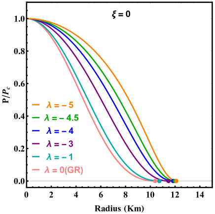
Figure 1: $P/P_{c}$ vs Radius curve of a single star for $\lambda=0$ (pure GR case),$-1,-3,-4,-4.5,-5$ with $\xi=0$

From Figure(1), we see that the relative pressure $P/P_{c}$ starts from $1$ (value at $r=0$), although evolves differently (corresponding to different $\lambda$ values) as a function of the radial distance, but eventually falls to zero value at $r=R$ where $R$ is the radius of the NS star. The circles(towards the end of each curve) with different colours give us the maximum radius of the NS in our given model corresponding to different $\lambda$ values. These are shown in column four of the table(1).

In figure (2) we have shown the total masses of the NS $M/M_{\odot}$ (normalized in solar mass) as a function of its radius $R$ for different values of $\lambda$ corresponding to $\rho_{c}=1.5\times 10^{18}kg/m^{3}$. For $\lambda=0$(normal GR case - the lowermost pink curve), we find that the mass point(denoted by a full circle) $1.06M_{\odot}$(the maximum mass) with radius of $10.409$ km. We see that as we decrement the value of $\lambda$(more negative $\lambda$ value), the maximum mass value of the NS also increases (as shown in table(1)).

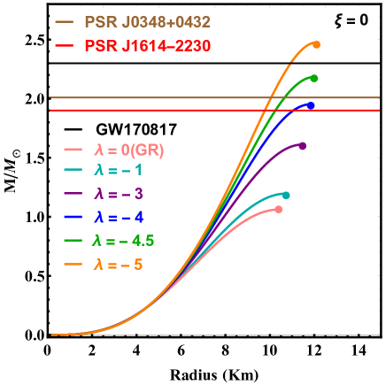
Figure 2: Mass vs Radius curve of a single star for $\lambda=0$ (pure GR case),$-1,-3,-4,-4.5,-5$ with $\xi=0$

In table (1), we have shown the the maximum mass point (mass of the NS) and radius of the NS for each different value of $\lambda$. For smaller values of $\lambda=-1,-3,-5$, we find the maximum mass of the NS as $M=1.19M_{\odot}$, $1.61M_{\odot}$ and $2.47~{}M_{\odot}$ corresponding to the radius($R$) $10.737$ km, $11.461$ km and $12.119$ km., respectively.

As shown in figure (2), taking the maximum mass of the first Binary Neutron Star (BNS) merger detected by LIGO i.e. GW170817 of maximum mass [102, 103] $\approx$ $2.33\smash{\scriptstyle\pm}0.17M_{\odot}$ $\&$ radius $10.4\smash{\scriptstyle\pm}0.14$ km , the mass-radius data of pulsars PSRJ1614–2230 (It’s a Millisecond Pulsar detected by NICER in 2018) [104] of mass ($1.908\smash{\scriptstyle\pm}0.016M_{\odot}$) $\&$ radius($10.30\sim 9.67$ km) and PSR J0348+0432 detected by Radio Telescope [105] in 2013 of mass ($2.01\smash{\scriptstyle\pm}0.04M_{\odot}$) $\&$ radius ($12.957\sim 12.246$ km) as the observational constraints, we got for only values of $\lambda=-4,-4.5,-5$ the mass-radius curve cross the constraint of PSR J1614–2230 of mass (denoted by the red horizontal line), both PSR J1614-2230 $\&$ PSR J0348+0432(denoted by brown horizontal line) and all 3 constraints i.e PSR J1614–2230, PSR J0348+0432 $\&$ GW170817(denoted by black horizontal line) respectively.

MGT parameters		Single Star
$\lambda$	$\xi$	$M_{\text{max}}(M_{\odot})$	$R(km)$
0	0	1.06	10.409
-1	0	1.19	10.737
-3	0	1.61	11.461
-4	0	1.95	11.830
-4.5	0	2.18	11.994
-5	0	2.47	12.119

Table 1: Table of $M_{\text{max}}(M_{\odot})$ and $R(km)$ for a single star and number of stars with $\xi=0$

To give more robust information regarding the mass-radius curve, how $\lambda=-4,-4.5.-5$ crossing the $3$ given observation constraints(only one, two and all three) respectively, is shown in the table(2).

Values	Observational Constraints
$\lambda$	PSRJ$1614$	PSRJ$0348$	GW$170817$
-4	Y	N	N
-4.5	Y	Y	N
-5	Y	Y	Y

Table 2: Table of intersection of $M_{\text{max}}(M_{\odot})$ - $R(km)$ curve for a single star with observational constraints for $\xi=0$

Figure 3: $P/P_{c}$ vs radius curve for $\lambda=-7$ diverges, not tends to zero at the surface

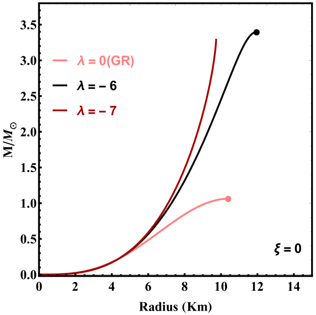
Figure 4: Mass vs Radius curve of a single stars for $\lambda=-7$

While tuning the parameters according to values of$\lambda$, we also focus on the maximum values of modified gravity parameter $|\lambda|$at which the physical system of curves breaks down i.e. the curves diverge not come to zero at the surface($r=R$). We find the value of $\lambda=-7$, the curve diverges upward - the stability criteria $\partial M/\partial R<0$ (in general for any star system) is not satisfied - which is required to be satisfied for a neutron star system.

Figure 5: Mass($M/M_{\odot}$) vs Radius($R$) curves of a single stars for $\lambda=-6$ for different $\rho_{c}$( $10^{18}kg/m^{3}$

For $\lambda=-6$ as the maximum mass, the radius limit which is satisfied by a stellar mass Black Hole ( Mass above $\approx$ $3M_{\odot}$) shown in figures (4, 4).

We next see how the central energy density $\rho_{c}$ plays an important role in the solutions of the TOV equations. Taking the values of $\rho_{c}$ = $1.1,1.2,1.3,1.4,1.5,1.6$ ( $\times 10^{18}kg/m^{3}$), we find the mass-radius, pressure - radius plots for $\lambda=-6$ (and $\xi=0$) (Even though it gives maximum mass above $3M_{\odot}$, it is also solvable for spherical symmetric metric ), which are shown in figures (5) and (6) respectively.

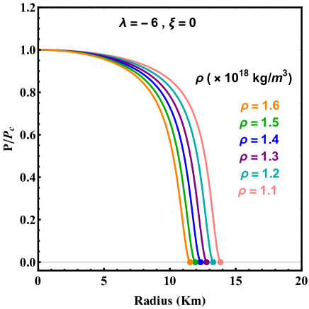
Figure 6: $P/P_{c}$ vs radius curves for $\lambda=-6$ for different $\rho_{c}$( $10^{18}kg/m^{3}$)

From figure (5), we find that, as the central energy density $\rho_{c}$ increases from $1.1(\times 10^{18}kg/m^{3})$ to $1.6(\times 10^{18}kg/m^{3})$,

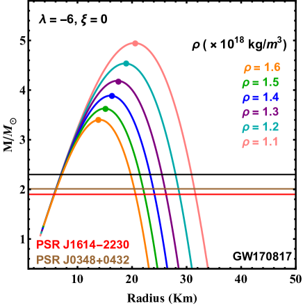
Figure 7: Mass vs Radius curves of number of stars for $\lambda=-6$ for different $\rho_{c}$( $10^{18}kg/m^{3}$ ), where each dot represents the maximum limit

the maximum mass point $M_{\rm{max}}$ decreases from $4.19~{}M_{\odot}$ to $3.23~{}M_{\odot}$, while the radius $R$ decreases from $13.86$ km to $11.54$ km. The limitation is such that we can’t decrease the values $\rho_{c}$ to such a low value which won’t satisfy the physical region of mass-radius of neutron star(above $3M_{\odot}$ it will be a black hole.

Similarly, when we increase the value of $\rho_{c}=1.6\times 10^{18}kg/m^{3}$, the curve becomes shorter and compact compared to the original taken $\rho_{c}\approx 1.5(\times 10^{18}kg/m^{3})$. So, beyond that value, we didn’t get approachable plots suitable for Neutron star study.

In fig. (7), the mass-radius curves of the number of stars for $\lambda(\lambda_{max})=-6$ are studied corresponding to different $\rho_{c}$ values.

The coloured dots on the curves represent the maximum mass point and radius which is increasing(decreasing) depending on decreasing(increasing) the value of $\rho_{c}$ from $1.1$ to $1.6$ ($\times 10^{18}kg/m^{3}$) from our taken $\rho_{c}$ value.

We will extend the above analysis with a small non-zero value of $\xi$(where $\xi\simeq 10^{-27}$) and see how the results in this non-minimal scenario($\lambda\neq 0,~{}\xi\neq 0$) gets changed from the minimal scenario (where $\lambda\neq 0,~{}\xi=0$).

• Case II: $R+2\lambda T+\xi T^{2}$ Model:

We investigate the behaviour of the neutron star system by incorporating an additional free parameter referred to as $\xi$ with $R+2\lambda T+\xi T^{2}$.

Using the same polytropic EoS $P=K\rho^{\gamma}$ with $\gamma,K$ as before, we solve the TOV EoS for neutron star matter corresponding to different $\lambda$ and $\xi$ values.

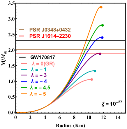
Figure 8: Mass vs Radius curve of a single star for $\lambda=0$ (pure GR case),$-1,-3,-4,-4.5,-5$ with $\xi=10^{-27}$

In figure (8) we have shown the total masses of the NS $M/M_{\odot}$ (normalized in solar mass) as a function of its radius $R$ for $\lambda=0,-1,-3,-4,-4.5,-5$ and $\xi=10^{-27}$ corresponding to $\rho_{c}=1.5\times 10^{18}kg/m^{3}$. The pink curve represents the mass-radius curve in pure GR($\lambda=0,~{}\xi=0$) of having maximum mass piont(denoted by a full circle) $1.06M_{\odot}$ and Radius of $10.409$ km. Compared to previous models the values of $\lambda=-3$ just touched the observational constraints like pulsar data of PSRJ$1614-2230$ of mass ($1.90M_{\odot}$). But, $\lambda=-4,-4.5$ with $\xi=10^{-27}$ satisfy all he given observation constraints maximum mass bound i.e Binary Neutron Star Merger GW$170817$ max. mass [102, 103] of $2.33M_{\odot}$, pulsar data of PSRJ$1614-2230$ of mass ($1.90M_{\odot}$) [104] and PSRJ$0348+0432$ of mass ($2.01M_{\odot}$) [105]. But, the value of Radius decreased for higher values of $\lambda=-4.5,-5$ to $11.88$ km, $11.68$km even though the maximum mass of the system reached to $2.80M_{\odot}$ and $3.39M_{\odot}$.

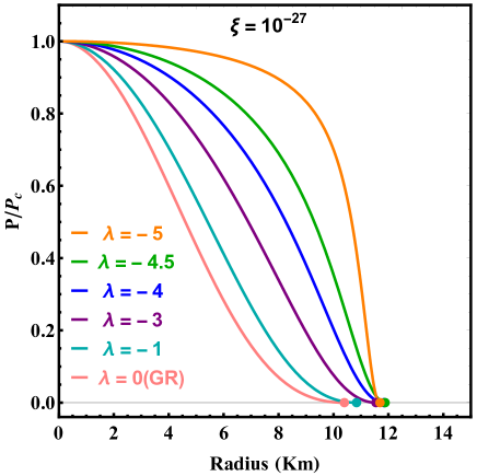
Figure 9: $P/P_{c}$ vs Radius curve of a single star for $\lambda=0$ (pure GR case),$-1,-3,-4,-4.5,-5$ with $\xi=10^{-27}$

Similar to the previous analysis, we have also analyzed the behaviour of $P/P_{c}$ with the radius $R$, considering the EoS $P=K\rho^{\gamma}$ (and $P_{c}=K\rho_{c}^{\gamma}$) corresponding to different $\lambda$ values and $\xi\approx 10^{-27}$ values and the results are graphically presented in Figure (9). Although the variation of relative pressure i.e.($P/P_{c}$) with radius starts from the same point, the curves meet at higher values of radius axis, represented by the full circles with different colours, signifying the increase in the maximum radius of the star due to the presence of the additional modified gravity parameter $\xi$, where at the surface $r=R$, the pressure always vanishes to zero.

MGT parameters		Single Star
$\lambda$	$\xi$	$M_{\text{max}}(M_{\odot})$	$R(km)$
0	0	1.06	10.409
-1	$10^{-27}$	1.34	10.843
-3	$10^{-27}$	1.89	11.549
-4	$10^{-27}$	2.41	11.838
-4.5	$10^{-27}$	2.80	11.885
-5	$10^{-27}$	3.39	11.680

Table 3: Table of $M_{\text{max}}(M_{\odot})$ and $R(km)$ for a single star and number of stars with $\xi=10^{-27}$

Interestingly, with $\lambda\neq 0,\xi\neq 0$, we see that the results surpass the 3 given observational constraints at integer value of $\lambda=-4$ ( which in case of $f(R,T)=R+2\lambda T$ model, we got this for $\lambda=-5$).

In Table (3), we have displayed the maximum mass and radius of the NS for different $\lambda$ values with $\xi\approx 10^{-27}$.

From Figure (8) and Table (3), we found that the pink curve that represents the mass-radius curve in pure GR, corresponds to maximum mass point(denoted by a full circle) $1.06M_{\odot}$ and radius $R=10.409$ km.

In Table (4) , we have shown how the different $M-R$ curves with different values of $\lambda$ (-3,-4, -4.5, -5) with a small value of $\xi~{}(10^{-27})$ intersect with the three designated observational constraints.

Values	Observational Constraints
$\lambda$	PSRJ$1614$	PSRJ$0348$	GW$170817$
-3	Y*	N	N
-4	Y	Y	Y
-4.5	Y	Y	Y
-5	Y	Y	Y

Table 4: Table of intersection of $M_{\text{max}}(M_{\odot})$ - $R(km)$ curve for a single star with observational constraints for $\xi\neq 0$ (* means just touched the observational constraint PSRJ$1614-2230$)

We next identify the maximum values of $|\lambda|$ (with $\xi\neq 0$ ) at which the physical system of curves undergoes a breakdown, manifesting as a divergence rather than approaching zero at the surface ($r=R$). Notably, we pinpoint the critical value of $\lambda=-6$ (for the previous model the same was for $\lambda=-7$), where the curve exhibits an upward divergence—indicating a departure from the stability criterion $\partial M/\partial R<0$, a crucial condition for the stability of neutron star systems in general.

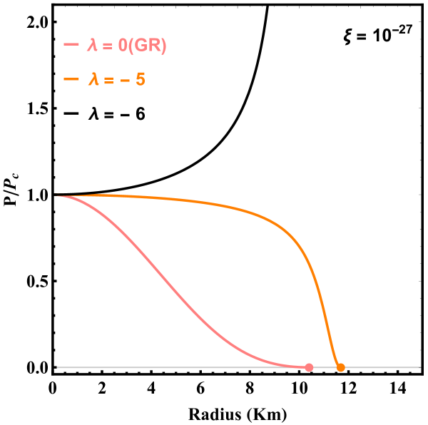
Figure 10: $P/P_{c}$ vs radius curve for $\lambda=-6$ diverges(with $\xi\neq 0$), not tends to zero at the surface

Figure 11: Mass vs Radius curve of a single stars for $\lambda=-6$ with $\xi\neq 0$

As we fixed the value of $\xi$ for different values of $\lambda$ for the second case(i.e. $R+2\lambda T+\xi T^{2}$), if we put $\xi=0$; the parameter $\lambda$ in equation (18), which relates to the stiffness of the Equation of State (EoS), is determined by the speed of sound($v_{s}$). The valid range of values for $\lambda$ is $-4\pi<\lambda\leq 0$ when the speed of sound ($v_{s}$) is within the range of $0$ to $1$ [101]. So, the range of $\lambda\sim 0~{}\rm{to}-5$ that we have chosen in our analysis, satisfies the above constraints as imposed by the speed of sound.

Figure 12: Mass($M/M_{\odot}$) vs Radius($R$) curves of a single stars for $\lambda=-5$ for different $\rho_{c}$( $10^{18}kg/m^{3}$ with $\xi\neq 0$

It is worthwhile to investigate the sensitivity of $M-R$ curve of the choice of the central density of the NS in the modified gravity scenario with $\lambda,~{}\xi\neq 0$.

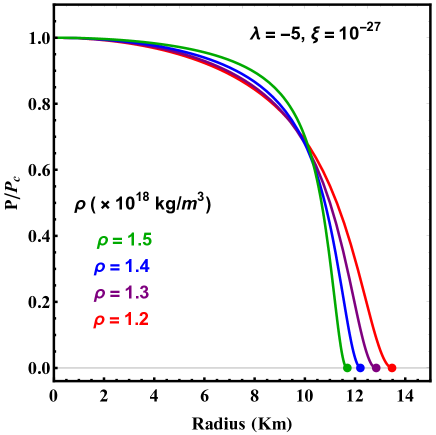
Figure 13: $P/P_{c}$ vs radius curves for $\lambda=-5$ for different $\rho_{c}$( $10^{18}kg/m^{3}$) with $\xi\neq 0$

For different central energy densities apart from $\rho_{c}=1.5(\times 10^{18}kg/m^{3}$), we also find the mass-radius and pressure-radius plots. Compared to the previous analysis (when $\xi=0$) for $\rho_{c}=1.1,1.6(\times 10^{18}kg/m^{3}$), the curves don’t satisfy the physical system of any compact star(Neutron Star or Black Hole). So, by decreasing the value of $\rho_{c}=1.5$ to $1.2(\times 10^{18}kg/m^{3})$, the maximum mass limit increased slowly from $3.39,3.43,3.51$ and $3.64M_{\odot}$ giving the existence of mass limit of Stellar-mass Black Hole ($\approx$ MASS above $3M_{\odot}$), shown in fig (12 )and the relative pressure ($P/P_{c}$) becomes zero for the higher value of $R_{surface}$ shown in fig (13).

In fig (14), the mass-radius plots for the number of neutron stars for different central energy densities $\rho_{c}$ described earlier for $\xi\neq 0$ model are studied for $\lambda=-5$. The coloured dots on the curves represent the maximum mass limit. Giving a minor increment in the maximum value of ( $M/M_{\odot}$ , $R$) limit on the curve for decreased value of $\rho_{c}=1.2\times 10^{18}kg/m^{3}$.

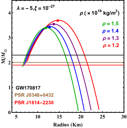
Figure 14: Mass vs Radius curves of number of stars for $\lambda=-5$ with $\xi=10^{-27}$ for different $\rho_{c}$( $10^{18}kg/m^{3}$ ), where each dot represents the maximum limit

VI.2 Likelihood Analysis of Physical Parameters

In above analysis, we have seen how the mass($M$), radius($R$), pressure($P$) and density($\rho$) of the neutron star depends on the modified gravity parameters $\lambda$ and $\xi$. Here, in addition, we have conducted a Markov Chain Monte Carlo (MCMC) [106, 107, 108] sampling for the purposes of estimating modified gravity parameters.

The essential procedure when running MCMC in this context involves comparing models generated using a specific set of parameters with observed data. These models are generated with the aim of finding a subset of parameters that produce models that best align with our observed data. The MCMC approach is fundamentally rooted in Bayesian statistics [109, 110], as opposed to the frequentist perspective. In practical terms, when using MCMC, we need to specify priors for our parameters. These priors serve as a way to incorporate our prior beliefs or knowledge as modellers about the system we’re analyzing into the modelling process.

We calculate the probability of our model given our specific data. In the terminology of statisticians, this value is expressed as, $P(\theta|D)$ (known as “posterior probability ”) and is calculated using Bayes theorem as [111],

$$P(\theta|D)=\dfrac{P(D|\theta)P(\theta)}{P(D)}$$ (20)

Here the terms are :

• $P(D|\theta)$: the probability of the data given the model (this is called the likelihood)

• $P(\theta)$: the probability of our model (known as the prior)

• $P(D)$: The probability of the data (often called the evidence)

Taking here $\theta=(\lambda,\xi)$ are modified gravity parameters and $D=(D_{GW},D_{PSR})$ where $D_{GW}=$GW$170817$ data, $D_{PSR}=$ PSRJ$0348+0432$ $\&$ PSRJ$1614-2230$ data are the sets of data from different types of observations to construct the likelihood. As the sample size is large enough, we use the Gaussian likelihood function (also known as Normal distribution which will obey the Central Limit theorem) defined as [112],

$$P(D|\theta)=\prod\limits^{3}_{k=1}\dfrac{1}{\sigma_{k}\sqrt{2\pi}}\exp{-\dfrac{1}{2}\left(\dfrac{D_{k}-M_{k}}{\sigma_{k}}\right)^{2}}$$ (21)

In equation (21) the index $k$ runs over all the data, $D_{k}$ and $M_{k}$ are the data and their corresponding model values respectively. The $\sigma_{k}$ is the standard deviation whose square gives the variance.

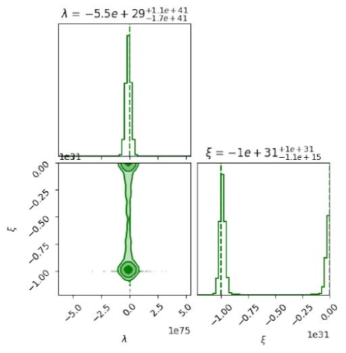
Figure 15: Corner plot of the posterior distribution of modified gravity parameters

Keeping in mind all the above conditions, the posterior distribution of modified gravity parameters $\lambda$ and $\xi$; is shown in the figure (15) :

From figure(15), we found that after running the samplers up to 10000 steps we got the posterior distribution function of $\lambda$ and $\xi$ taking the range of $\lambda$ = $(-5.0,5.0)$ and $\xi=(-1.0,0.0)$. The vertical green line shows the median of the posterior distribution with the lower bound of $-1.7e+41$, $-1.1e+15$ and upper bound of $1.1e+41$, $1e+31$ of the $68\%$ (1$\sigma$) credible interval(CI) for the parameters $\lambda$ $\&$ $\xi$ respectively.

Figure 16: Corner plot of the posterior distribution of Radius(R), Mass($M/M_{\odot}$) in our taken modified gravity $f(R,T)=R+h(T)$ with 3 given observational constraints

Taking our observational constraints i.e. GW170817 (BNS Merger) mass - radius data, observed pulsars PSRJ$1614-2230$, PSRJ$0348+0432$ maximum mass; we found that posterior distribution plot of mass $\&$ radius which is shown in next figure (16).

In figure(16), the 1D marginalized posterior distribution plots of mass($M/M_{\odot}$) $\&$ Radius($R$) taking only GW$170817$ data is shown in the blue curve, where the lower bound of $68$ $\%$ CI($1\sigma$ region) overlap with the same plot of adding GW$170817$ data with PSRJ$0348+0432$ as likelihood (which represents as the red vertical line ) and it completely differs when we take 3 data as the likelihood (GW$170817$ + PSRJ$0348+0432$ + PSRJ$1614-2230$) as shown in the green vertical lines for the mass. For the radius, the upper bound of $68$ $\%$ CI mostly overlaps with each other for 3 different cases as mentioned earlier. The contour plot of the 2D marginalized posterior distribution of the mass-radius for the 3 datasets depicts that only GW170817 data overcomes the remaining 2 contour plots (red and green) when we added the 2 PSR data. So, overall the $1\sigma$, $2\sigma$, and $3\sigma$ regions of each curve coincide with each other giving the maximum mass to $2.03$ $M_{\odot}$ with $+0.43$ $\&$ $-0.49$ error value and maximum radius to be $11.01$ km with $+0.89$ $\&$ $-0.85$ error values.

VI.3 Correlation Study among Different Parameters

We also explore how different values of $\lambda$ and $\xi$ impact the correlations among various physical parameters of neutron stars such as mass($M$), radius($R$), pressure($P$) and energy density($\rho$). These correlations are visualized in figure (17):

Figure 17: Correlation coefficients of different NS observables in $f(R,T)$ gravity with different sets of $\lambda$ and $\xi$

From this study, we draw the following conclusions :

1. $M_{max}$ is strongly correlated with $R$ i.e ($>0.9$), that with $\rho_{c}$ is weak ( $\sim 0.028$). But $P$ and $M_{max}$ show moderate correlation ($0.4$).

2. $P$ is moderately correlated with $R$ ($\sim 0.53$), also the same with $\rho_{c}$ is very very less ($-0.02\approx 0$) at the surface pressure becomes zero.

3. $R$ is also weakly correlated with $\rho_{c}$ i.e (0.055)

VII Conclusions

In this work, we study the equilibrium configuration of the Neutron Star in a modified gravity approach. We calculate the various observable properties of neutron stars based on a polytropic model $P=K\rho^{\gamma}$ in a modified $f(R,T)=R+2\lambda T+\xi T^{2}$ gravity theory where $\lambda,\xi$ are the modified gravity parameters.

For $\lambda=-5$, we found that the $f(R,T)=R+2\lambda T$ model satisfies all the theoretical/observational constraints. Note that the choice of $\lambda$, that we have made in our analysis i.e. $-4\pi<\lambda\leq 0$ is determined by the fact that the speed of sound $v_{s}$ should satisfy $0<v_{s}/c<1$.

With the quadratic term in $T$ in $f(R,T)=R+2\lambda T+\xi T^{2}$ model, we find that the model satisfies all the constraints for $\lambda=-4$ corresponding to a fixed value of $\xi=10^{-27}$. which is comparable with the existing results available in the literature.

So, for a range of values of $\lambda$ with $\xi=0(\neq 0)$, we found that the mass $M$ and the radius $R$ of the NS lie within the range given by the GW170817 gravitational wave data given by LIGO, Pulsars (Rapidly Rotating Neutron Stars) (PSR) data and the NICER (Neutron star Interior Composition ExploreR) mass-radius data given by NASA.

We also obtain the bound on the modified gravity parameter $\lambda$ from the mass instability and analyzed how the maximum mass point $M_{\rm{max}}$ and the radius $R$ depends on the central energy density $\rho_{c}$ of the NS. With $\lambda=-6,~{}\xi=0$, we found that as the central core density($\rho_{c}$) increases from $1.1\times 10^{18}~{}\rm{kg~{}m^{-3}}$ to $1.6\times 10^{18}~{}\rm{kg~{}m^{-3}}$, the maximum mass point $M_{\rm{max}}$ of the NS decreases from $4.19\times M_{\odot}$ to $3.23\times M_{\odot}$, while its radius $R$ decreases from $13.86$ km to $11.54$ km(So, the choice of energy density is an important factor in deciding the fate of a compact star either it will be a Neutron Star / Black Hole).

Taking the observational constraints i.e. GW170817 (BNS Merger) mass - radius data, observed pulsars PSRJ1614-2230, PSRJ0348+0432 maximum mass, radius data; we found that posterior distribution plot of Mass $\&$ Radius gives good result and the corner plot of modified gravity parameters $\lambda$ and $\xi$ are giving very good posterior results. We studied how the modified gravity parameters $\lambda$ and $\xi$ impact the correlations between various physical parameters of neutron stars such as mass $M$, radius $R$, pressure $P$ and energy density $\rho$. $M_{max}$ is strongly correlated with $R$ i.e ($>0.9$), that with $\rho_{c}$ is weak ( $\sim 0.028$). But $P$ and $M_{max}$ show moderate correlation ($0.4$).Whereas $P$ is moderately correlated with $R$ ($\sim 0.53$), also the same with $\rho_{c}$ is very very less ($\sim-0.02\approx 0$) signifying the pressure vanishes at the surface and becomes zero.

VIII Acknowledgment

P. Mahapatra would like to thank BITS Pilani K K Birla Goa campus for providing a good computational facility for this project and fellowship support. We thank Dr. Ajith Parameswaran (ICTS, Bangalore) $\&$ Dr. Akshay Rana (Delhi University) for the useful discussions regarding MCMC sampling and insightful comments on this work. We thank Dr. Subhadip Sau (Jhargram Raj College, Jhargram, West Bengal) for some relevant ideas regarding the plot and comments on our EoS. P K Das would like to thank Dr. Madhukar Mishra of BITS Pilani, Pilani campus for several useful discussions related to Neutron Star.

References

- Einstein [1915] A. Einstein, The Field Equations of Gravitation, Sitzungsber. Preuss. Akad. Wiss. Berlin (Math. Phys. ) 1915, 844 (1915).
- Coley and Wiltshire [2017] A. A. Coley and D. L. Wiltshire, What is General Relativity?, Phys. Scripta 92, 053001 (2017), arXiv:1612.09309 [gr-qc] .
- Sahni [2004] V. Sahni, Dark matter and dark energy, Lect. Notes Phys. 653, 141 (2004), arXiv:astro-ph/0403324 .
- Khuri [2003] R. R. Khuri, Dark matter as dark energy, Phys. Lett. B 568, 8 (2003), arXiv:astro-ph/0303422 .
- Kamionkowski [2007] M. Kamionkowski, Dark Matter and Dark Energy, in Amazing Light: Visions for Discovery: An International Symposium in Honor of the 90th Birthday Years of Charles H. Townes (2007) arXiv:0706.2986 [astro-ph] .
- van de Bruck et al. [2023] C. van de Bruck, G. Poulot, and E. M. Teixeira, Scalar field dark matter and dark energy: a hybrid model for the dark sector, JCAP 07, 019, arXiv:2211.13653 [hep-th] .
- Farnes [2018] J. S. Farnes, A unifying theory of dark energy and dark matter: Negative masses and matter creation within a modified CDM framework, Astron. Astrophys. 620, A92 (2018), arXiv:1712.07962 [physics.gen-ph] .
- Katsuragawa and Matsuzaki [2017] T. Katsuragawa and S. Matsuzaki, Dark matter in modified gravity?, Phys. Rev. D 95, 044040 (2017), arXiv:1610.01016 [gr-qc] .
- Perlmutter et al. [1998] S. Perlmutter et al. (Supernova Cosmology Project), Discovery of a supernova explosion at half the age of the Universe and its cosmological implications, Nature 391, 51 (1998), arXiv:astro-ph/9712212 .
- Riess et al. [1998] A. G. Riess et al. (Supernova Search Team), Observational evidence from supernovae for an accelerating universe and a cosmological constant, Astron. J. 116, 1009 (1998), arXiv:astro-ph/9805201 .
- Riess et al. [1999] A. G. Riess et al., BV RI light curves for 22 type Ia supernovae, Astron. J. 117, 707 (1999), arXiv:astro-ph/9810291 .
- Ade et al. [2014] P. A. R. Ade et al. (Planck), Planck 2013 results. XVI. Cosmological parameters, Astron. Astrophys. 571, A16 (2014), arXiv:1303.5076 [astro-ph.CO] .
- Adam et al. [2016] R. Adam et al. (Planck), Planck 2015 results. I. Overview of products and scientific results, Astron. Astrophys. 594, A1 (2016), arXiv:1502.01582 [astro-ph.CO] .
- Peebles [1980] P. J. E. Peebles, The large-scale structure of the universe (1980).
- Bartelmann and Maturi [2016] M. Bartelmann and M. Maturi, Weak gravitational lensing (2016) arXiv:1612.06535 [astro-ph.CO] .
- Munshi et al. [2008] D. Munshi, P. Valageas, L. Van Waerbeke, and A. Heavens, Cosmology with Weak Lensing Surveys, Phys. Rept. 462, 67 (2008), arXiv:astro-ph/0612667 .
- Yamamoto et al. [2023] M. Yamamoto, M. A. Troxel, M. Jarvis, R. Mandelbaum, C. Hirata, H. Long, A. Choi, and T. Zhang, Weak gravitational lensing shear estimation with metacalibration for the Roman High-Latitude Imaging Survey, Mon. Not. Roy. Astron. Soc. 519, 4241 (2023), arXiv:2203.08845 [astro-ph.IM] .
- Penton et al. [2000] S. V. Penton, J. T. Stocke, and J. M. Shull, The local lyman-alpha forest. I: observations with the ghrs/g160m on the hubble space telescope, Astrophys. J. Suppl. 130, 121 (2000), arXiv:astro-ph/9911117 .
- Liddle [2004] A. R. Liddle, How many cosmological parameters?, Mon. Not. Roy. Astron. Soc. 351, L49 (2004), arXiv:astro-ph/0401198 .
- Li et al. [2011] M. Li, X.-D. Li, S. Wang, and Y. Wang, Dark Energy, Commun. Theor. Phys. 56, 525 (2011), arXiv:1103.5870 [astro-ph.CO] .
- Dodelson et al. [1996] S. Dodelson, E. I. Gates, and M. S. Turner, Cold dark matter models, Science 274, 69 (1996), arXiv:astro-ph/9603081 .
- Armendariz-Picon and Neelakanta [2014] C. Armendariz-Picon and J. T. Neelakanta, How Cold is Cold Dark Matter?, JCAP 03, 049, arXiv:1309.6971 [astro-ph.CO] .
- Hu et al. [2000] W. Hu, R. Barkana, and A. Gruzinov, Cold and fuzzy dark matter, Phys. Rev. Lett. 85, 1158 (2000), arXiv:astro-ph/0003365 .
- Weinberg et al. [2015] D. H. Weinberg, J. S. Bullock, F. Governato, R. Kuzio de Naray, and A. H. G. Peter, Cold dark matter: controversies on small scales, Proc. Nat. Acad. Sci. 112, 12249 (2015), arXiv:1306.0913 [astro-ph.CO] .
- Sigurdson [2009] K. Sigurdson, Hidden Hot Dark Matter as Cold Dark Matter, (2009), arXiv:0912.2346 [astro-ph.CO] .
- Taylor and Silk [2003] J. E. Taylor and J. Silk, The Clumpiness of cold dark matter: Implications for the annihilation signal, Mon. Not. Roy. Astron. Soc. 339, 505 (2003), arXiv:astro-ph/0207299 .
- Roszkowski et al. [2018] L. Roszkowski, E. M. Sessolo, and S. Trojanowski, WIMP dark matter candidates and searches—current status and future prospects, Rept. Prog. Phys. 81, 066201 (2018), arXiv:1707.06277 [hep-ph] .
- Hirsch et al. [2013] M. Hirsch, R. A. Lineros, S. Morisi, J. Palacio, N. Rojas, and J. W. F. Valle, WIMP dark matter as radiative neutrino mass messenger, JHEP 10, 149, arXiv:1307.8134 [hep-ph] .
- Bottaro et al. [2022] S. Bottaro, D. Buttazzo, M. Costa, R. Franceschini, P. Panci, D. Redigolo, and L. Vittorio, Closing the window on WIMP Dark Matter, Eur. Phys. J. C 82, 31 (2022), arXiv:2107.09688 [hep-ph] .
- Saikawa and Shirai [2020] K. Saikawa and S. Shirai, Precise WIMP Dark Matter Abundance and Standard Model Thermodynamics, JCAP 08, 011, arXiv:2005.03544 [hep-ph] .
- Bertone et al. [2018] G. Bertone, N. Bozorgnia, J. S. Kim, S. Liem, C. McCabe, S. Otten, and R. Ruiz de Austri, Identifying WIMP dark matter from particle and astroparticle data, JCAP 03, 026, arXiv:1712.04793 [hep-ph] .
- Graesser et al. [2011] M. L. Graesser, I. M. Shoemaker, and L. Vecchi, Asymmetric WIMP dark matter, JHEP 10, 110, arXiv:1103.2771 [hep-ph] .
- Adams et al. [2022] C. B. Adams et al., Axion Dark Matter, in Snowmass 2021 (2022) arXiv:2203.14923 [hep-ex] .
- Chadha-Day et al. [2022] F. Chadha-Day, J. Ellis, and D. J. E. Marsh, Axion dark matter: What is it and why now?, Sci. Adv. 8, abj3618 (2022), arXiv:2105.01406 [hep-ph] .
- Duffy and van Bibber [2009] L. D. Duffy and K. van Bibber, Axions as Dark Matter Particles, New J. Phys. 11, 105008 (2009), arXiv:0904.3346 [hep-ph] .
- Semertzidis and Youn [2022] Y. K. Semertzidis and S. Youn, Axion dark matter: How to see it?, Sci. Adv. 8, abm9928 (2022), arXiv:2104.14831 [hep-ph] .
- Panci et al. [2023] P. Panci, D. Redigolo, T. Schwetz, and R. Ziegler, Axion dark matter from lepton flavor-violating decays, Phys. Lett. B 841, 137919 (2023), arXiv:2209.03371 [hep-ph] .
- Stern [2015] I. P. Stern, Axion Dark Matter Searches, AIP Conf. Proc. 1604, 456 (2015), arXiv:1403.5332 [physics.ins-det] .
- Fleury and Moore [2016] L. Fleury and G. D. Moore, Axion dark matter: strings and their cores, JCAP 01, 004, arXiv:1509.00026 [hep-ph] .
- Yang [2017] Q. Yang, Axions and dark matter, Mod. Phys. Lett. A 32, 1740003 (2017), arXiv:1509.00673 [hep-ph] .
- Condon and Matthews [2018] J. J. Condon and A. M. Matthews, CDM Cosmology for Astronomers, Publ. Astron. Soc. Pac. 130, 073001 (2018), arXiv:1804.10047 [astro-ph.CO] .
- Anselmi et al. [2023] S. Anselmi, M. F. Carney, J. T. Giblin, S. Kumar, J. B. Mertens, M. O’Dwyer, G. D. Starkman, and C. Tian, What is flat CDM, and may we choose it?, JCAP 02, 049, arXiv:2207.06547 [astro-ph.CO] .
- Turner [2018] M. S. Turner, CDM: Much More Than We Expected, but Now Less Than What We Want, Found. Phys. 48, 1261 (2018), arXiv:2109.01760 [astro-ph.CO] .
- Bull et al. [2016] P. Bull et al., Beyond CDM: Problems, solutions, and the road ahead, Phys. Dark Univ. 12, 56 (2016), arXiv:1512.05356 [astro-ph.CO] .
- Perivolaropoulos and Skara [2022] L. Perivolaropoulos and F. Skara, Challenges for CDM: An update, New Astron. Rev. 95, 101659 (2022), arXiv:2105.05208 [astro-ph.CO] .
- Ghosh et al. [2023] S. Ghosh, P. Jain, R. Kothari, M. Panwar, G. Singh, and P. Tiwari, Probing cosmology beyond CDM using SKA, J. Astrophys. Astron. 44, 22 (2023), arXiv:2301.03065 [astro-ph.CO] .
- Clifton [2006] T. Clifton, Alternative theories of gravity, Other thesis (2006), arXiv:gr-qc/0610071 .
- Dodelson and Liguori [2006] S. Dodelson and M. Liguori, Can Cosmic Structure form without Dark Matter?, Phys. Rev. Lett. 97, 231301 (2006), arXiv:astro-ph/0608602 .
- Casanellas et al. [2012] J. Casanellas, P. Pani, I. Lopes, and V. Cardoso, Testing alternative theories of gravity using the Sun, Astrophys. J. 745, 15 (2012), arXiv:1109.0249 [astro-ph.SR] .
- Bekenstein [2010] J. D. Bekenstein, Alternatives to Dark Matter: Modified Gravity as an Alternative to dark Matter, , 99 (2010), arXiv:1001.3876 [astro-ph.CO] .
- Hehl [1997] F. W. Hehl, Alternative gravitational theories in four-dimensions, in 8th Marcel Grossmann Meeting on Recent Developments in Theoretical and Experimental General Relativity, Gravitation and Relativistic Field Theories (MG 8) (1997) pp. 423–432, arXiv:gr-qc/9712096 .
- Alex and Reinhart [2020] N. Alex and T. Reinhart, Covariant constructive gravity: A step-by-step guide towards alternative theories of gravity, Phys. Rev. D 101, 084025 (2020), arXiv:1909.03842 [gr-qc] .
- Bauer et al. [2022] A. M. Bauer, A. Cárdenas-Avendaño, C. F. Gammie, and N. Yunes, Spherical Accretion in Alternative Theories of Gravity, Astrophys. J. 925, 119 (2022), arXiv:2111.02178 [gr-qc] .
- De Laurentis et al. [2016] M. De Laurentis, O. Porth, L. Bovard, B. Ahmedov, and A. Abdujabbarov, Constraining alternative theories of gravity using GW and GW, Phys. Rev. D 94, 124038 (2016), arXiv:1611.05766 [gr-qc] .
- Esposito-Farese [2019] G. Esposito-Farese, Hamiltonian vs stability in alternative theories of gravity, in 54th Rencontres de Moriond on Gravitation (2019) arXiv:1905.04586 [gr-qc] .
- Moffat [2004] J. W. Moffat, Modified gravitational theory as an alternative to dark energy and dark matter, (2004), arXiv:astro-ph/0403266 .
- Zlosnik et al. [2007] T. G. Zlosnik, P. G. Ferreira, and G. D. Starkman, Modifying gravity with the Aether: An alternative to Dark Matter, Phys. Rev. D 75, 044017 (2007), arXiv:astro-ph/0607411 .
- Shankaranarayanan and Johnson [2022] S. Shankaranarayanan and J. P. Johnson, Modified theories of gravity: Why, how and what?, Gen. Rel. Grav. 54, 44 (2022), arXiv:2204.06533 [gr-qc] .
- Reyes and Schreck [2022] C. M. Reyes and M. Schreck, Modified-gravity theories with nondynamical background fields, Phys. Rev. D 106, 044050 (2022).
- Boehmer and Jensko [2021] C. G. Boehmer and E. Jensko, Modified gravity: A unified approach, Phys. Rev. D 104, 024010 (2021), arXiv:2103.15906 [gr-qc] .
- Nojiri et al. [2017a] S. Nojiri, S. D. Odintsov, and V. K. Oikonomou, Modified Gravity Theories on a Nutshell: Inflation, Bounce and Late-time Evolution, Phys. Rept. 692, 1 (2017a), arXiv:1705.11098 [gr-qc] .
- Bahamonde et al. [2015] S. Bahamonde, C. G. Böhmer, and M. Wright, Modified teleparallel theories of gravity, Phys. Rev. D 92, 104042 (2015), arXiv:1508.05120 [gr-qc] .
- Hirano and Fujita [2022] S. Hirano and T. Fujita, Effective Field Theory of Large Scale Structure in modified gravity and application to Degenerate Higher-Order Scalar-Tensor theories, (2022), arXiv:2210.00772 [gr-qc] .
- Clifton et al. [2012] T. Clifton, P. G. Ferreira, A. Padilla, and C. Skordis, Modified Gravity and Cosmology, Phys. Rept. 513, 1 (2012), arXiv:1106.2476 [astro-ph.CO] .
- Mandal et al. [2021] R. Mandal, D. Saha, M. Alam, and A. K. Sanyal, Early Universe in view of a modified theory of gravity, Class. Quant. Grav. 38, 025001 (2021), arXiv:2101.02851 [hep-th] .
- Lobo [2008] F. S. N. Lobo, The Dark side of gravity: Modified theories of gravity, (2008), arXiv:0807.1640 [gr-qc] .
- Olmo et al. [2020] G. J. Olmo, D. Rubiera-Garcia, and A. Wojnar, Stellar structure models in modified theories of gravity: Lessons and challenges, Phys. Rept. 876, 1 (2020), arXiv:1912.05202 [gr-qc] .
- Roussille [2022] H. Roussille, Black hole perturbations in modified gravity theories, Ph.D. thesis, Diderot U., Paris (2022), arXiv:2211.01103 [gr-qc] .
- Olmo et al. [2019] G. J. Olmo, D. Rubiera-García, and A. Wojnar, Stellar structure models in modified theories of gravity: Lessons and challenges, Physics Reports (2019).
- Chang and Hui [2011] P. Chang and L. Hui, Stellar Structure and Tests of Modified Gravity, Astrophys. J. 732, 25 (2011), arXiv:1011.4107 [astro-ph.CO] .
- Wojnar [2022] A. Wojnar, Stellar and substellar objects in modified gravity (2022) arXiv:2205.08160 [gr-qc] .
- Sakstein [2013] J. Sakstein, Stellar Oscillations in Modified Gravity, Phys. Rev. D 88, 124013 (2013), arXiv:1309.0495 [astro-ph.CO] .
- Tonosaki et al. [2023] S. Tonosaki, T. Tachinami, and Y. Sendouda, Nonrelativistic stellar structure in higher-curvature gravity: Systematic construction of solutions to the modified Lane-Emden equations, Phys. Rev. D 108, 024037 (2023), arXiv:2303.03853 [gr-qc] .
- Lopez Armengol and Romero [2017] F. G. Lopez Armengol and G. E. Romero, Neutron stars in Scalar-Tensor-Vector Gravity, Gen. Rel. Grav. 49, 27 (2017), arXiv:1611.05721 [gr-qc] .
- Mathew et al. [2020] A. Mathew, M. Shafeeque, and M. K. Nandy, Stellar structure of quark stars in a modified Starobinsky gravity, Eur. Phys. J. C 80, 615 (2020), arXiv:2006.06421 [gr-qc] .
- Abbott et al. [2017] B. P. Abbott et al. (LIGO Scientific, Virgo), GW170817: Observation of Gravitational Waves from a Binary Neutron Star Inspiral, Phys. Rev. Lett. 119, 161101 (2017), arXiv:1710.05832 [gr-qc] .
- Moffat [2020] J. W. Moffat, Modified Gravity (MOG) and Heavy Neutron Star in Mass Gap, (2020), arXiv:2008.04404 [gr-qc] .
- Glendenning [1996] N. Glendenning, Compact Stars. Nuclear Physics, Particle Physics and General Relativity. (1996).
- Lattimer and Prakash [2004] J. M. Lattimer and M. Prakash, The physics of neutron stars, Science 304, 536 (2004), arXiv:astro-ph/0405262 .
- Kunz [2023] J. Kunz, Neutron Stars, Lect. Notes Phys. 1017, 293 (2023), arXiv:2204.12520 [gr-qc] .
- Alford et al. [2022] M. G. Alford, L. Brodie, A. Haber, and I. Tews, Relativistic mean-field theories for neutron-star physics based on chiral effective field theory, Phys. Rev. C 106, 055804 (2022), arXiv:2205.10283 [nucl-th] .
- Piekarewicz [2022] J. Piekarewicz, The Nuclear Physics of Neutron Stars, (2022), arXiv:2209.14877 [nucl-th] .
- Nättilä and Kajava [2022] J. Nättilä and J. J. E. Kajava, Fundamental physics with neutron stars, in Handbook of X-ray and Gamma-ray Astrophysics, edited by C. Bambi and A. Santangelo (2022) arXiv:2211.15721 [astro-ph.HE] .
- Özel and Freire [2016] F. Özel and P. Freire, Masses, Radii, and the Equation of State of Neutron Stars, Ann. Rev. Astron. Astrophys. 54, 401 (2016), arXiv:1603.02698 [astro-ph.HE] .
- Fraga et al. [2016] E. S. Fraga, A. Kurkela, and A. Vuorinen, Neutron star structure from QCD, Eur. Phys. J. A 52, 49 (2016), arXiv:1508.05019 [nucl-th] .
- Sotani and Togashi [2022] H. Sotani and H. Togashi, Neutron star mass formula with nuclear saturation parameters, Phys. Rev. D 105, 063010 (2022), arXiv:2203.09004 [nucl-th] .
- Trautmann et al. [2016] W. Trautmann, M. D. Cozma, and P. Russotto, Symmetry energy and density, PoS Bormio2016, 036 (2016), arXiv:1610.03650 [nucl-ex] .
- Abbassi [2001] A. H. Abbassi, General Birkhoff’s theorem, (2001), arXiv:gr-qc/0103103 .
- Schleich and Witt [2009] K. Schleich and D. M. Witt, What does Birkhoff’s theorem really tell us?, (2009), arXiv:0910.5194 [gr-qc] .
- Harko et al. [2011] T. Harko, F. S. N. Lobo, S. Nojiri, and S. D. Odintsov, gravity, Phys. Rev. D 84, 024020 (2011), arXiv:1104.2669 [gr-qc] .
- Tretyakov [2018] P. V. Tretyakov, Cosmology in modified -gravity, Eur. Phys. J. C 78, 896 (2018), arXiv:1810.11313 [gr-qc] .
- Ashmita et al. [2022] Ashmita, P. Sarkar, and P. K. Das, Inflationary cosmology in the modified f (R, T) gravity, Int. J. Mod. Phys. D 31, 2250120 (2022), arXiv:2208.11042 [gr-qc] .
- Arora et al. [2021] S. Arora, S. Bhattacharjee, and P. K. Sahoo, Late-time viscous cosmology in gravity, New Astron. 82, 101452 (2021), arXiv:2007.06790 [gr-qc] .
- Deb and Deshamukhya [2022] B. Deb and A. Deshamukhya, Constraining logarithmic model using Dark Energy density parameter and Hubble parameter , in 23rd International Conference on General Relativity and Gravitation (2022) arXiv:2207.10610 [gr-qc] .
- Sotiriou and Faraoni [2010] T. P. Sotiriou and V. Faraoni, f(R) Theories Of Gravity, Rev. Mod. Phys. 82, 451 (2010), arXiv:0805.1726 [gr-qc] .
- De Felice and Tsujikawa [2010] A. De Felice and S. Tsujikawa, f(R) theories, Living Rev. Rel. 13, 3 (2010), arXiv:1002.4928 [gr-qc] .
- Nojiri et al. [2017b] S. Nojiri, S. D. Odintsov, and V. K. Oikonomou, Constant-roll inflation in f(r) gravity, Classical and Quantum Gravity 34, 245012 (2017b).
- Carvalho et al. [2017] G. A. Carvalho, R. V. Lobato, P. H. R. S. Moraes, J. D. V. Arbañil, R. M. Marinho, E. Otoniel, and M. Malheiro, Stellar equilibrium configurations of white dwarfs in the f(R, T) gravity, Eur. Phys. J. C 77, 871 (2017), arXiv:1706.03596 [gr-qc] .
- Moraes et al. [2018] P. H. R. S. Moraes, J. D. V. Arbañil, G. A. Carvalho, R. V. Lobato, E. Otoniel, R. M. Marinho, and M. Malheiro, Compact Astrophysical Objects in gravity, in 14th International Workshop on Hadron Physics (2018) arXiv:1806.04123 [gr-qc] .
- Pretel et al. [2021] J. M. Z. Pretel, S. E. Jorás, R. R. R. Reis, and J. D. V. Arbañil, Neutron stars in gravity with conserved energy-momentum tensor: Hydrostatic equilibrium and asteroseismology, JCAP 08, 055, arXiv:2105.07573 [gr-qc] .
- Lobato et al. [2020] R. Lobato, O. Lourenço, P. H. R. S. Moraes, C. H. Lenzi, M. de Avellar, W. de Paula, M. Dutra, and M. Malheiro, Neutron stars in ) gravity using realistic equations of state in the light of massive pulsars and GW170817, JCAP 12, 039, arXiv:2009.04696 [astro-ph.HE] .
- Nathanail et al. [2021] A. Nathanail, E. R. Most, and L. Rezzolla, GW170817 and GW190814: tension on the maximum mass, Astrophys. J. Lett. 908, L28 (2021), arXiv:2101.01735 [astro-ph.HE] .
- Shibata et al. [2019] M. Shibata, E. Zhou, K. Kiuchi, and S. Fujibayashi, Constraint on the maximum mass of neutron stars using GW170817 event, Phys. Rev. D 100, 023015 (2019), arXiv:1905.03656 [astro-ph.HE] .
- Takisa et al. [2014] P. M. Takisa, S. Ray, and S. D. Maharaj, Charged compact objects in the linear regime, Astrophys. Space Sci. 350, 733 (2014), arXiv:1412.8121 [gr-qc] .
- Zhao [2016] X.-F. Zhao, On the moment of inertia of PSR J0348+0432, Chin. J. Phys. 54, 839 (2016), arXiv:1712.08852 [nucl-th] .
- Speagle [2019] J. S. Speagle, A Conceptual Introduction to Markov Chain Monte Carlo Methods, arXiv e-prints , arXiv:1909.12313 (2019), arXiv:1909.12313 [stat.OT] .
- Joseph [2019] A. Joseph, Markov Chain Monte Carlo Methods in Quantum Field Theories: A Modern Primer (Springer, 2019) arXiv:1912.10997 [hep-th] .
- Buchanan et al. [2023] J. J. Buchanan, M. D. Schneider, K. Pruett, and R. E. Armstrong, Markov chain monte carlo for bayesian parametric galaxy modeling in lsst (2023), arXiv:2309.10321 [astro-ph.IM] .
- Sharma [2017] S. Sharma, Markov chain monte carlo methods for bayesian data analysis in astronomy, Annual Review of Astronomy and Astrophysics 55, 213 (2017).
- Ottosen [2012] T. A. Ottosen, Markov-chain monte-carlo a bayesian approach to statistical mechanics (2012), arXiv:1206.6905 [astro-ph.GA] .
- Robert et al. [2010] C. P. Robert, J.-M. Marin, and J. Rousseau, Bayesian inference (2010), arXiv:1002.2080 [stat.ME] .
- Trotta [2008] R. Trotta, Bayes in the sky: Bayesian inference and model selection in cosmology, Contemp. Phys. 49, 71 (2008), arXiv:0803.4089 [astro-ph] .