Ascending the attractor flow in the D1-D5 system

Abstract

We study maximally supersymmetric irrelevant deformations of the D1-D5 CFT that correspond to following the attractor flow in reverse in the dual half-BPS black string solutions of type IIB supergravity on K3. When a single, quadratic condition is imposed on the parameters of the $22$ such irrelevant deformations, the asymptotics of the solution degenerate to a linear dilaton-like spacetime. We identify each such degeneration limit with a known decoupling limit of string theory, which yields little string theory or deformations thereof (the so-called open brane LST, or OD$p$ theories), compactified to two dimensions. This suggests that a $21$-parameter family of the above deformations leads to UV-complete theories, which are string theories decoupled from gravity that are continuously connected to each other. All these theories have been argued to display Hagedorn behaviour; we show that including the F1 strings leads to an additional Cardy term. The resulting entropy formula closely resembles that of single-trace $T\bar{T}$-deformed CFTs, whose generalisations could provide possibly tractable effective two-dimensional descriptions of the above web of theories.

We also consider the asymptotically flat black strings. At fixed temperature, the partition function is dominated by thermodynamically stable, ‘small’ black string solutions, similar to the ones in the decoupled backgrounds. We show that certain asymptotic symmetries of these black strings bear a striking resemblance with the state-dependent symmetries of single-trace $T\bar{T}$, and break down precisely when the background solution reaches the ‘large’ black string threshold. This suggests that small, asymptotically flat black strings may also admit a $T\bar{T}$ - like effective description.

1 Introduction

Finding a microscopic explanation for the entropy of general black holes has been a main driving force of research in quantum gravity, ever since Bekenstein and Hawking’s discovery that black holes are thermodynamic systems [1, 2, 3]. The AdS/CFT correspondence [4] marked a significant advance in this direction, as it provided a microscopic explanation of the entropy of large black holes in anti de-Sitter spacetimes in terms of the thermal entropy in the dual CFT [5]. In AdS₃/CFT₂, the coefficient of the entropy can be matched exactly [6].

Central to the derivation of the AdS/CFT correspondence is the existence of a decoupling limit, which ensures a separation between the open and closed string descriptions of the brane system. This limit is a low-energy one, in which the open string description flows to a CFT and the closed string modes are confined to an AdS throat, where their redshift is nearly infinite. There are, however, many other decoupling limits known within string theory, which relate non-local field theories [7, 8] or string theories decoupled from gravity [9, 10, 11, 12, 14, 13, 15, 16] to space-times with non-AdS asymptotics. It is all but natural, if one seeks to understand the entropy black holes with non-AdS asymptotics - such as, for example, asymptotically flat black holes - to consider these more general instances of holography.

In this article, we concentrate on the D1-D5 system, which consists of a stack of D5 branes wrapped on K3 (for specificity; we could have equally considered $T^{4}$) and D1 branes parallel to their remaining worldvolume direction. This system has been very extensively studied (see [17] and references therein). At zero temperature and angular potential, its supergravity description is as a half-BPS black string in type IIB supergravity compactified on K3. We will be studying both this supersymmetric solution and its non-extremal version.

The supersymmetric black string is well-known to exhibit an attractor mechanism [18, 19, 20], whereby a subset of the moduli at infinity must reach prespecified values at the horizon, which are determined by the charges of the black string. More specifically, for type IIB supergravity on K3, the massless scalars at infinity parametrise the coset

$$\mathcal{M}_{\infty}=\frac{SO(5,21)}{SO(5)\times SO(21)}$$ (1.1)

Upon flowing to the near-horizon region, $21$ of the initial $105$ massless scalar fields acquire a mass from the AdS₃ point of view [21] and their values become fixed. From the perspective of the D1-D5 CFT that describes the near-horizon region, the $21$ attracted scalars correspond to single-trace irrelevant operators of left/right conformal dimension $(2,2)$; one additional such irrelevant operator is related to changes in the size of the AdS₃ and $S^{3}$. The moduli space of the near-horizon region, parametrised by the remaining massless scalars, is locally the coset

$$\mathcal{M}_{hor}=\frac{SO(4,21)}{SO(4)\times SO(21)}$$ (1.2)

and coincides with the moduli space of the D1-D5 CFT [22].

Given the standard identification between the radial direction in the bulk and the energy scale in the boundary theory, as well as between the supergravity moduli and the coupling constants on the brane worldvolume, the attractor flow may be seen, from the boundary perspective, as a flow towards low energies that ends at an IR fixed point [23]. $22$ of the couplings of the original theory become irrelevant in the IR. The corresponding picture is sketched in the figure below.

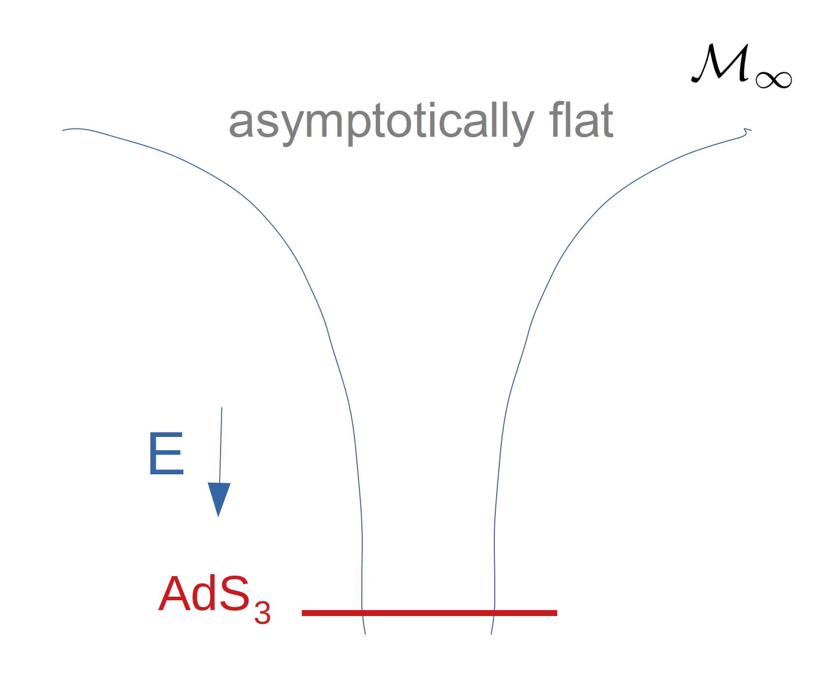
(a)

(b)

Figure 1: The attractor flow corresponds to a flow towards low energies, both in the gravity picture (left), where one nears the AdS₃ throat of the black string, and in the boundary one (right), where one flows towards an IR CFT fixed point (red dot). The moduli spaces of the near-horizon region (red line) and of the CFT are identified and are given by (1.2).

One may verify this picture infinitesimally around the attractor point, by matching the maximally supersymmetric single-trace irrelevant operators to the leading departure of the black string solution away from the near-horizon one, as well as the connection for these operators over the CFT moduli space to the connection on the normal bundle of (1.2) inside (1.1) [23].

The framework of this article consists of looking at this picture in reverse (figure 2), whereby we map the inverse attractor flow out of the AdS${}_{3}\times S^{3}$ near-horizon region - which should eventually bring us to flat space - to a $22$ - parameter family of maximally supersymmetric irrelevant deformations of the D1-D5 CFT. As already explained, these deformations start as $(2,2)$ irrelevant operators near the IR fixed point and may, in principle, receive many corrections as one flows upwards in energy. The question we would like to address herein is:

Q:  What type of theory does one obtain for finite values of the irrelevant couplings?

In general, following an irrelevant deformation to higher orders in (conformal) perturbation theory is a very difficult and possibly ill-defined task, due to the proliferation of unfixed counterterms. However, there is some hope that the particular deformations above may be tractable, as maximal supersymmetry severely restricts the other operators that may appear, at least in the supergravity limit. Such an approach was put forth in [24] for D3 branes, and has been recently revisited in [25], but has yet to yield non-trivial predictions.

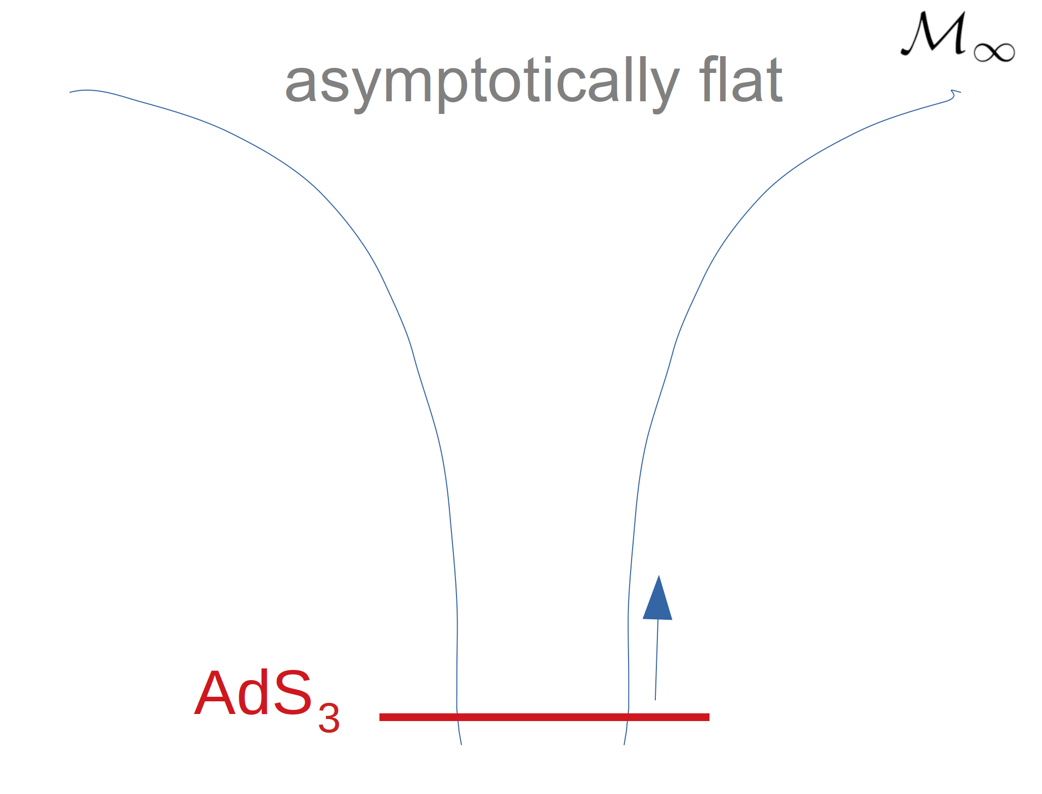
(a)

(b)

Figure 2: The reverse attractor flow is mapped to turning on irrelevant deformations in the D1-D5 CFT. Reaching out (to) a finite distance outside the throat corresponds to understanding the boundary theory at finite values of the irrelevant couplings.

The recent example of exactly solvable finite irrelevant deformations of two-dimensional QFTs [26] has given renewed hope of solving this problem. The resulting theories appear to be UV-complete [27] and intrinsically non-local at the scale set by the irrelevant deformation parameter. The best-studied examples of such theories are $T\bar{T}$ - deformed CFTs [26, 28], which are Lorentz invariant, and $J\bar{T}$ - deformed CFTs [29], which are Lorentz-breaking, but preserve the standard conformal symmetries and locality along one lightlike direction. Both classes of theories share many features with standard, local two-dimensional CFTs, such as the presence of Virasoro generators [30, 32, 33, 31] and correlation functions that are related in a simple, universal, albeit non-local manner to standard CFT₂ correlators [34, 35, 36]. As argued in [33], the natural basis for the extended symmetry generators is a Fourier one, in which the symmetry algebra becomes a $T\bar{T}$/$J\bar{T}$ - specific non-linear deformation of the Virasoro $\times$ Virasoro algebra. There also exists a ‘single-trace’ generalisation of $T\bar{T}$- and $J\bar{T}$-deformed CFTs [37, 40, 38, 39], which simply denotes the symmetric product orbifold of the above theories. The universal structure of the deformed spectrum and correlation functions, as well as the infinite symmetries, carries over from the double-trace case, in a completely predictable fashion [40] (for the spectrum, see also [41]).

An interesting connection between $T\bar{T}$ deformations and non-AdS holography has been put forth in [37], who showed that the asymptotically linear dilaton (henceforth ALD) spacetime one obtains in the NS5 decoupling limit (namely $g_{s}\rightarrow 0$, keeping $\alpha^{\prime}$ fixed) of the NS5-F1 system shares many features with a single-trace $T\bar{T}$ - deformed CFT. To be more precise, the spacetime obtained in this decoupling limit interpolates between an AdS₃ region in the IR and a linear dilaton one in the UV, and thus its holographic description is precisely that of an irrelevant flow out of a CFT; on the boundary side, the decoupling limit yields LST, a non-local, non-gravitational theory with string-like excitations [9] compactified on K3 or $T^{4}$, whose size is assumed to be much smaller than that of the IR AdS₃. Research in this subfield has followed two main strands: the first one concerns the worldsheet string theory description of the decoupled spacetime, which exhibits a perfect match between the spectrum and correlation functions of long string states/operators in this background and their $T\bar{T}$ - deformed counterparts. Thus, there is very good evidence that the long string subsector of string theory in this background is described by a symmetric product orbifold if $T\bar{T}$ - deformed CFTs. This subsector does not, however, dominate the entropy [42]. On the other hand, the short string spectrum and correlators do not match the $T\bar{T}$ ones, thus precluding an exact duality between string theory in the ALD blackground and single-trace $T\bar{T}$ (except perhaps for the case of a single NS5-brane [43, 44]).

The second strand of results connect universal quantities in the decoupled linear dilaton spacetime - which are, in principle, defined throughout the moduli space and carry information about the entire theory - and single-trace $T\bar{T}$. One such observable is the entropy. In [37], it was shown that the entropy of black holes in the ALD spacetime precisely matches the single-trace $T\bar{T}$ - deformed entropy, which has a characteristic Cardy $\rightarrow$ Hagedorn behaviour

$$S=2\pi\sqrt{\frac{c}{3}(pER+\mu E^{2})}$$ (1.3)

where $c$ is the central charge of the seed $CFT$, $p$ is the number of copies in the symmetric orbifold and $\mu$ is the dimensionful coupling. We have set the momentum to zero, for simplicity.

Another important piece of evidence for a universal connection between the two is that the asymptotic symmetry group of the ALD spacetime precisely matches [45] the particular non-linear modification of the Virasoro algebra that represents the symmetry algebra of single-trace $T\bar{T}$ - deformed CFTs [40]. Given that the holographic dual of the ALD spacetime cannot be the exact symmetric product orbifold of $T\bar{T}$ - deformed CFTs, these results point towards the existence of generalisations of single-trace $T\bar{T}$ - deformed CFTs that share the same behaviour of the entropy and the extended symmetries. How to define the appropriate generalisations is is an interesting question for future research.

The NS5-F1 system discussed above is just a particular case of the general half-BPS black string solutions mentioned at the beginning of this section, where the only moduli that are turned on are the dilaton and the overall volume of the internal manifold. The six-dimensional dilaton is an attracted scalar, and thus the black string geometry corresponds to turning on the corresponding irrelevant deformation, denoted $\lambda_{-}$, in the D1-D5 CFT. The size of the $AdS_{3}$ also grows when moving out of the near-horizon region, and its associated deformation parameter is $\lambda_{+}\geq|\lambda_{-}|$. In a convenient normalisation, the NS5 decoupling limit then corresponds to the particular case in which

$$\lambda_{+}=\lambda_{-}=\alpha^{\prime}k$$ (1.4)

where $\alpha^{\prime}k$ is the effective irrelevant coupling, with $k$ the number of NS5 branes. Even though this result is extracted from an infinitesimal analysis (at small $\alpha^{\prime}$), the existence of the UV-complete LST description for finite $\alpha^{\prime}$ indicates that there should be a sense in which the irrelevant deformations (1.4) can be turned on a finite amount. This viewpoint is supported by the fact that the deformation is nearly exact in the supergravity regime, and that its $T\bar{T}$ effective description also exists at the corresponding finite value of the irrelevant parameter. In the following, we will be using the terminology “irrelevant coupling” and “supergravity parameter” interchangeably.

One of the main goals of this article is to argue that this picture extends to the full moduli space of the D1-D5 system. Namely, we show that all instances in which the asymptotics of the general half-BPS black string solution degenerate to an ALD-like spacetime - which happens on a codimension one subspace of the moduli space at infinity - correspond to a known decoupling limit of string theory. We thus expect that the irrelevant deformations whose coefficients satisfy the corresponding field-theoretical constraint yield a UV-complete theory (see figure 3). These deformations span a $21$-dimensional subspace of the $22$ possible maximally supersymmetric irrelevant deformations of the system. The remaining irrelevant direction turns on the deformation to six-dimensional asymptotically flat space, for which a rigorous decoupling limit is not known.

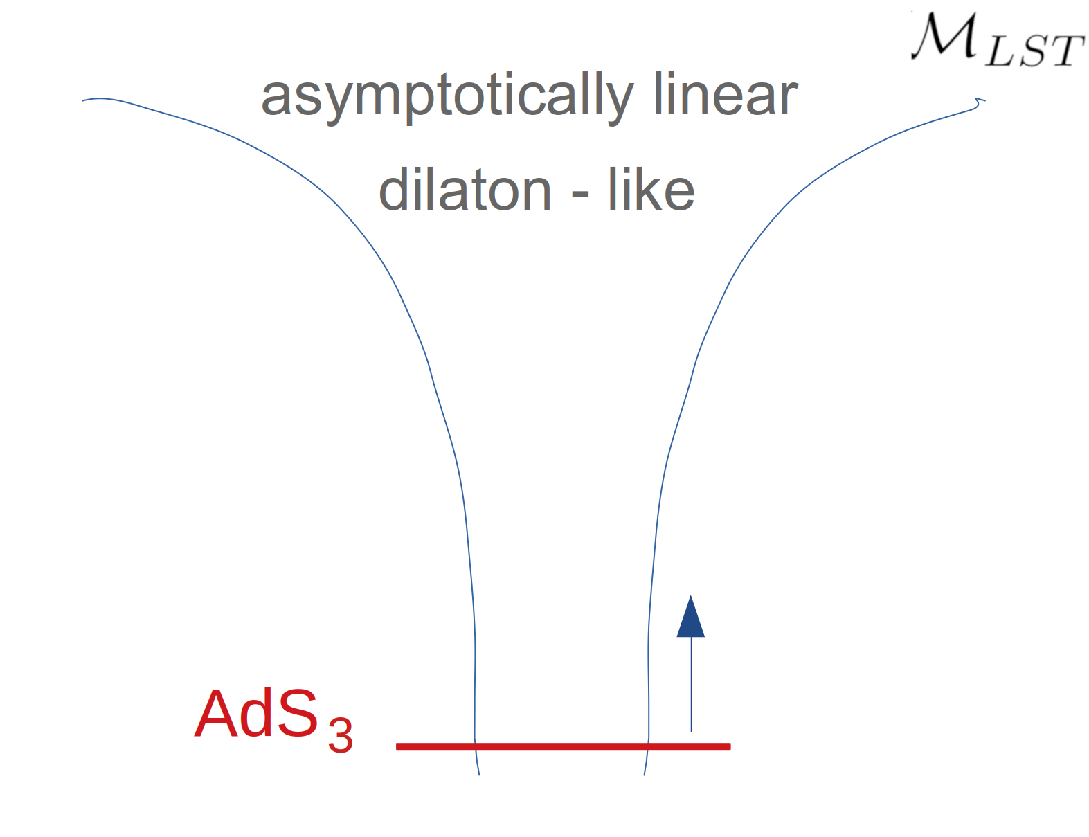
(a)

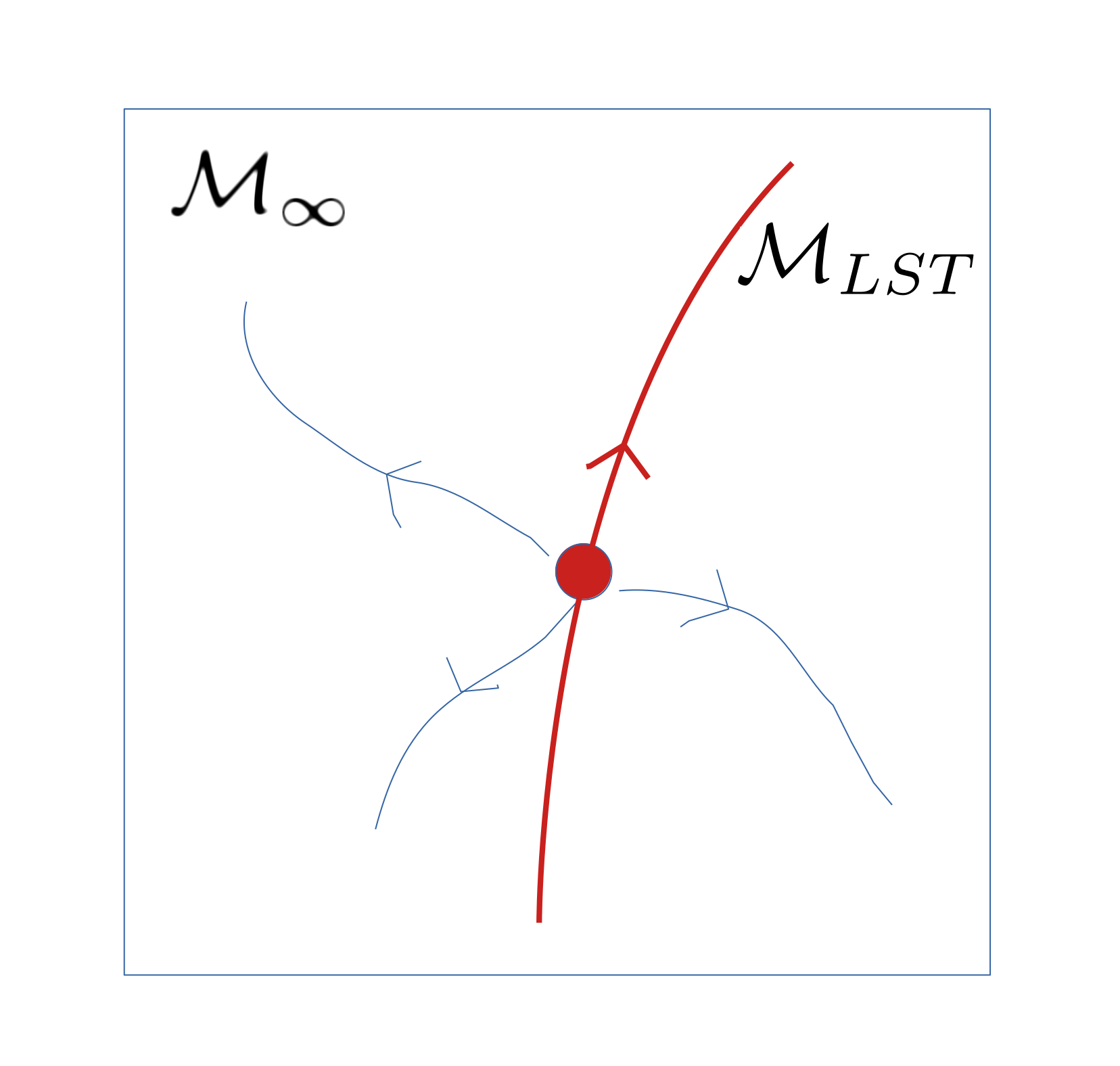
(b)

Figure 3: The asymptotics of the black string solutions degenerate on a codimension one subspace of the moduli space at infinity. This subspace is shown to be spanned by known decoupling limits of string theory, which yield little string theory and deformations thereof. It corresponds to turning on $21$ of the possible $22$ maximally supersymmetric irrelevant couplings.

The corresponding UV-complete theory is LST for the pure NS5-F1 system; in the remaining cases, it will be a deformed version thereof known as open brane LST (OBLST, or OD$p$, for $p=1,3$) [15, 16], all compactified on K3. These theories were discovered in the context of understanding non-trivial decoupling limits of D-branes in a background Kalb-Ramond field. If the $B$-field is magnetic, then the decoupling limit yields a non-commutative deformation of the super Yang-Mills theory that describes the low-energy dynamics of the brane [7]. If it is electric, on the other hand, then the resulting theory is a space-time non-commutative open string theory (NCOS) that is decoupled from closed strings [12, 13]. The NCOS description is only valid at weak coupling; in particular, its associated Hagedorn behaviour cannot be seen in supergravity [12, 14]. The strong coupling limit of the D5 NCOS of interest to us is obtained via type IIB S-duality and is known as the OD$1$ theory; the OD$3$ ones are obtained by two further T-dualities [15]. It follows from this construction that the OD$p$/OBLST theories correspond to decoupling limits of NS5 branes in a background critical RR field, which in our case is either a two-form gauge field along the black string worldvolume (for OD$1$) or a four-form gauge field with two legs along one of the 19 anti-self-dual two-cycles of the K3 (for OD$3$).

All these decoupled theories are non-local and have closed (little) string excitations and generically also open D-branes; it is sometimes said they are space-time non-commutative, in the sense that they are S-dual to the space-time non-commutative NCOS. They are connected to each other via the web of dualities we briefly sketched; specific representatives may be obtained in particular limits of the coupling space, denoted as $\mathcal{M}_{LST}$ in the figure above. These couplings are related to ratios of the various irrelevant deformation coefficients that can be read off the supergravity description. Thus, our (partial) answer to the question raised at the beginning is

A:     When restricted to a codimension one subspace of the moduli space, the irrelevant deformations lead to a UV-complete theory which is, generically, a deformation of little string theory compactified on K3.

Infinitesimally away from this subspace, we can identify the remaining supergravity parameter with the coefficient of the irrelevant deformation that turns on the deformation to flat space; however, we still do not have a clear picture of what the resulting worldvolume theory is at finite values of this parameter.

Most of the above-mentioned theories are strongly-coupled and do not have a tractable worldvolume description. One may use, however, the dual gravitational description to infer some of their properties. In LST, it is well-known that the little strings lead to Hagedorn behaviour at high energies [11, 46, 47] which, as reviewed above, becomes Cardy $\rightarrow$ Hagedorn behaviour in presence of the F1s. In the literature, it has been argued that all the $ODp$/OBLST theories also exhibit Hagedorn behaviour at high energies; working under the same assumptions, we show that this behaviour becomes Cardy $\rightarrow$ Hagedorn upon the inclusion of the F1 strings, with a dependence on the parameters that is, again, very similar to that of single-trace $T\bar{T}$. Thus, all the theories that live on the codimension one subspace of the moduli space spanned by these decoupling limits appear to exhibit $T\bar{T}$ - like behaviour in their entropy, which is presumably associated to the universal presence of little strings. Whether their connection to $T\bar{T}$ is deeper than this may be investigated by - for example - computing the asymptotic symmetry groups of the associated spacetimes.

With respect to the original asymptotically flat region, all the black strings responsible for the behaviour above are near-extremal. It is, nevertheless, interesting to also discuss non-extremal asymptotically flat black strings from this perspective. One puzzling aspect of such black strings is, of course, that they are thermodynamically unstable. If one works in the canonical ensemble, it is however possible to show, following the entirely analogous analysis of [48] of non-extremal D3-branes, that at any fixed temperature below a certain maximum one, the pure NS5-F1 system contains two possible black string solutions: one, whose horizon is larger than a certain radius $r_{0}^{*}$, and one that is smaller (see figure 4). The large black string is thermodynamically unstable, but also has higher free energy than the small one, which is stable. The canonical ensemble is thus dominated by the small black string. One interesting feature we find in the NS5-F1 system with respect to the D3 one is that now the maximum size of the small black string can be made much larger than the size of the near-horizon AdS₃, thanks to a tunable coupling.

It appears reasonable to conjecture that the entropy of the small black string may be reproduced by a boundary theory with Hagedorn-like behaviour, as suggested by the existence of a maximal temperature in this system. As they do not dominate the thermal ensemble, large black strings are in a way similar to the small black holes in global AdS_D>3, but differ from them in that their entropy is larger than the maximum entropy that can be associated with just the open strings.

Motivated by the possibility to describe at least the small asymptotically flat black strings holographically, we study their asymptotic symmetries from this “$T\bar{T}$ perspective”, which suggests that the dual theory lives along the directions parallel to the string. We therefore concentrate on the dependence of the asymptotic Killing vectors on the black string coordinates, ignoring their dependence on the asymptotic $S^{3}$ coordinates. The resulting problem can be studied within a very simple three-dimensional consistent truncation of the non-extremal black string. Remarkably, we find that the asymptotic symmetry generators are extremely similar to those of the ALD spacetime [45] and thus single-trace $T\bar{T}$, as they correspond to field-dependent generalisations of conformal transformations. Interestingly, their background-dependent expressions break down precisely when the maximum size of the small black strings is reached, suggesting that a $T\bar{T}$ - like effective description is valid only below the associated maximum energy.

To summarize, the global picture that we arrrive at is that turning on $21$ of the $22$ possible maximally supersymmetric irrelevant deformations of the D1-D5 system for a finite amount leads to a UV-complete theory, which is in general a deformation of little string theory. The entropy of black holes in these theories appears to correspond to the thermal entropy of (little) strings, displaying a Cardy $\to$ Hagedorn behaviour that is also characteristic of single-trace $T\bar{T}$ - deformed CFTs. Thus, all the theories on this submanifold of the moduli space at infinity display $T\bar{T}$ - like features, without exactly being a symmetric product orbifold of $T\bar{T}$ - deformed CFTs, which suggests the existence of a “$T\bar{T}$ universality class” of two-dimensional QFTs. We also provided some evidence that the stable branch of asymptotically flat black strings may also fit within such a description, despite the fact that open and closed string modes in asymptotically flat space may not be fully decoupled.

This article is organised as follows. In section 2, we review the relevant black string solutions and the relationship between the attractor flow and irrelevant deformations of the D1-D5 CFT. In section 3, we link the asymptotic decoupling limits of various black string backgrounds to known decoupling limits of string theory, for which we provide a brief review. Finally, in section 4 we analyse the thermodynamics and asymptotic symmetries of the non-extremal asymptotically flat backgrounds, as well as the thermodynamics of the decoupled ones. We end with a discussion and future directions in section 5. The many technical details of our various calculations are relegated to the three appendices.

2 Supergravity, attractors and irrelevant deformations

In this section, we review the construction of the half-BPS black string solutions of type IIB supergravity compactified on K3, as well as their relation to irrelevant deformations of the D1-D5 CFT.

More precisely, in subsection 2.1 we briefly review six-dimensional supergravity coupled to tensor multiplets. Then, in 2.2 we review the construction of half-BPS black string solutions in $(1,0)$ six-dimensional supergravity, mostly as a warm-up for the construction, in subsection 2.3, of the $(2,0)$ attractor solutions, whose parametrization we explain in detail. Finally, we review the relation between the attracted scalars and irrelevant deformations of the D1-D5 CFT. We also explain how to generate, in type IIB supergravity, a basis of solutions of interest from the simple D1-D5 or F1-NS5 solution.

2.1 Six-dimensional supergravity

Let us consider six-dimensional $(1,0)$ or $(2,0)$ supergravity coupled to $n$ tensor multiplets. In the $(1,0)$ theory, the gravity multiplet consists of the graviton, two left gravitini and one self-dual three-form field, while the tensor multiplets consist of one anti-self-dual tensor, two right fermions (‘tensorini’) and one scalar. In $(2,0)$ supergravity, the gravity multiplet contains the graviton, four gravitini and five self-dual three-form fields, whereas the tensor multiplet contains one anti-self-dual tensor, four fermions and five scalars. The resulting theories thus contain $P$ self-dual three-form fields and $Q$ anti-self-dual ones, where for $(1,0)$ theories, $P=1$ and $Q=n$, whereas for $(2,0)$ ones $P=5$ and $Q=21$, as required by anomaly cancellation [50]. In both cases - and equally so for the non-chiral supersymmetric six-dimensional theories - the scalars are described by a nonlinear sigma model whose target space is locally of the form $SO(P,Q)/SO(P)\times SO(Q)$. For more details, see [52].

The description of the non-linear model of scalars taking values in a quotient space $G/H$, with $G$ non-compact and $H$ its maximal compact subgroup, is well known [51]. Assuming that $H$ acts by left multiplication, we require that the theory be invariant under the following gauge transformations

$$g(x)\rightarrow h(x)g(x)\,,$$ (2.1)

with $g\in G$, and for any $h\in H$. We then use the gauge connection $Q_{\mu}$, valued in $\mathfrak{h}={\rm Lie}(H)$, to introduce the covariant derivative

$$D_{\mu}g=\partial_{\mu}g-Q_{\mu}g\,,$$ (2.2)

which transforms in the same way as $g$, provided $Q_{\mu}\rightarrow hQ_{\mu}h^{-1}+\partial_{\mu}hh^{-1}$. The gauge-invariant Lagrangian is then simply given by

$$\mathcal{L}_{\rm coset}=-\frac{1}{2}Tr\,[(D_{\mu}g\,g^{-1})^{2}]\,.$$ (2.3)

The variation of the Lagrangian with respect to the field $Q_{\mu}$, which appears with no derivatives, yields the constraint ${\rm Tr}[D^{\mu}g\,g^{-1}\delta Q_{\mu}]=0$, implying that

$$P_{\mu}\equiv\frac{1}{\sqrt{2}}D_{\mu}g\,g^{-1}$$ (2.4)

is in the orthogonal complement of $\mathfrak{h}$ inside $\mathfrak{g}={\rm Lie}(G)$. In other words, decomposing $\partial_{\mu}g\,g^{-1}\in\mathfrak{g}$ as

$$\partial_{\mu}g\,g^{-1}=Q_{\mu}+P_{\mu}\sqrt{2}$$ (2.5)

provides a concrete way to express the gauge connection $Q_{\mu}$ and the physical fields $P_{\mu}$ in terms of the group elements and their derivatives. Note the above decomposition is perfectly compatible with the gauge transformations.

The Lagrangian (2.3) also has a global symmetry, corresponding to the right-multiplication by a constant group element, i.e. $g(x)\rightarrow g(x)g_{0}$ with $g_{0}\in G$. However, this continuous symmetry of the low-energy supergravity theory is broken to its maximal discrete subgroup in the full string theory.

Particularising the discussion to our case of interest, we have $G=SO(P,Q)$, $H=SO(P)\times SO(Q)$. It is customary to parametrise the $SO(P,Q)$ group elements as $X_{i\Lambda},X_{\bar{\imath}\Lambda}$, where the lower case latin indices transform under the local $SO(P)$ or $SO(Q)$, while the upper case greek ones do so under the global $SO(P,Q)$; these fields are sometimes referred to as ‘vielbeine’ [53]. The $SO(P,Q)$ condition $g^{T}\eta g=\eta$ reads

$$X_{i\Lambda}X_{i\Sigma}-X_{\bar{\imath}\Lambda}X_{\bar{\imath}\Sigma}=\eta_{\Lambda\Sigma}$$ (2.6)

where summation over the repeated indices is understood, and $\eta_{\Lambda\Sigma}$ is a diagonal matrix whose first $P$ entries equal $1$, while the remaining $Q$ ones are $-1$. In addition to these $(P+Q)(P+Q+1)/2$ constraints on the original $(P+Q)^{2}$ fields, one needs to fix the gauge symmetry, leaving a total of $PQ$ physical scalars. Of course, $g^{T}$ is also a symmetric matrix, which leads to

$$X_{i\Lambda}X_{j}{}^{\Lambda}=\delta_{ij}\;,\;\;\;\;\;X_{i\Lambda}X_{\bar{\imath}}{}^{\Lambda}=0\;,\;\;\;\;\;X_{\bar{\imath}\Lambda}X_{\bar{\jmath}}{}^{\Lambda}=-\delta_{\bar{\imath}\bar{\jmath}}\,,$$ (2.7)

where the index $\Lambda$ is raised and lowered with $\eta$.

So far for the scalar manifold. As stated above, the theory contains also $P+Q$ three-form tensor fields, with field strengths $F^{\Lambda}=dA^{\Lambda}$, which satisfy the modified (anti)-self-duality condition

$$\mathcal{N}_{\Lambda\Sigma}\star F^{\Sigma}=\eta_{\Lambda\Sigma}F^{\Sigma}$$ (2.8)

Here we have introduced the matrix $\mathcal{N}=g^{T}g$, which can be written as

$$\mathcal{N}_{\Lambda\Sigma}=X_{i\Lambda}X_{i\Sigma}+X_{\bar{\imath}\Lambda}X_{\bar{\imath}\Sigma}$$ (2.9)

and can be thought of as a gauge kinetic term in a pseudo-action used to derive a set of equations of motion that are consistent with the self-duality condition above for the three-forms, see e.g. [54] for more details. Note that (2.8) implies that the electric and magnetic charges of black strings computed using these field strengths are equal up to a sign. The charges are defined as

$$q^{\Lambda}=\frac{1}{2\pi^{2}}\int_{S^{3}}F^{\Lambda}$$ (2.10)

and are integer-quantized. On the other hand, the combinations of field strengths that appear in the supersymmetry variations are

$$F^{+i}=X^{i}{}_{\Lambda}F^{\Lambda}\;,\;\;\;\;\;F^{-\bar{\imath}}=X^{\bar{\imath}}{}_{\Lambda}F^{\Lambda}$$ (2.11)

which are (anti)-self-dual in the usual sense - as follows from the properties of the matrix $\mathcal{N}$ - but satisfy modified Bianchi identities [54]. While we use the same letter, $F$, to denote both sets of three-form fields, it should be clear from the index structure which one we are referring to. One may also introduce the central charges

$$Z^{i}=X^{i}{}_{\Lambda}q^{\Lambda}\;,\;\;\;\;\;\;Z^{\bar{\imath}}=X^{\bar{\imath}}{}_{\Lambda}q^{\Lambda}\,,$$ (2.12)

which can be related to the $S^{3}$ integrals of the (anti)-self-dual fields (see e.g. [55] for a discussion of their meaning in the case of non-spherical solutions). The norms of these central charges are denoted

$$|Z_{+}|\equiv(Z^{i}Z^{i})^{\frac{1}{2}}\;,\;\;\;\;\;\;\;|Z_{-}|\equiv(Z^{\bar{\imath}}Z^{\bar{\imath}})^{\frac{1}{2}}$$ (2.13)

and they satisfy $|Z_{+}|^{2}-|Z_{-}|^{2}=q^{\Lambda}q_{\Lambda}$, where we used (2.7). The $SO(P)$ central charge $|Z_{+}|$ corresponds to the eigenvalue of the central charge of the supersymmetry algebra.

When $P=Q$, the numbers of self-dual and anti-self dual tensor fields are equal, hence it is possible to write down a standard action for the theory. Denoting the standard kinetic term for the $P$ three-form fields in the lagrangian by $\mathcal{G}$ and the axionic couplings by $\mathcal{B}$, the relation with $\mathcal{N}_{\Lambda\Sigma}$ is given by [56]

$$C^{T}\mathcal{N}C=\left(\begin{array}[]{cc}1&\mathcal{B}\\ 0&1\end{array}\right)\left(\begin{array}[]{cc}\mathcal{G}&0\\ 0&\mathcal{G}^{-1}\end{array}\right)\left(\begin{array}[]{cc}1&0\\ -\mathcal{B}&1\end{array}\right)\;,\;\;\;\;\;C=\frac{1}{\sqrt{2}}\left(\begin{array}[]{cc}1&1\\ -1&1\end{array}\right)\,.$$ (2.14)

While will always have $P\neq Q$ at the level of the full supergravity theory, this relation will nevertheless be useful as we will consider a (purely bosonic) consistent truncation that contains equal numbers of self-dual and anti-self-dual three-form components.

The main focus of this article is the $(2,0)$ theory obtained by compactifying type IIB supergravity on K3, which has $P=5$ and $Q=21$. There are thus $PQ=105$ masless scalars in this compactification. Of these, $80$ correspond to the moduli of the metric and the $B$-field on K3, which parametrize an $SO(4,20)/SO(4)\times SO(20)$ subspace of the moduli space. The remaining 25 moduli correspond to the compactification of the RR two-form field $C_{2}$ on the $22$ 2-cycles of the K3 the axion $\chi_{1}$, the dilaton, and the RR four-form compactified on the entire (unit) internal manifold, here denoted as $\chi_{2}$. In a convenient basis, the $SO(5,21)$ vielbein can be (schematically) written in terms of these fields as

$$g =\Omega_{4}^{T}\begin{pmatrix}e^{-\phi}&0&0&0&0\\ -e^{\phi}(\chi_{1}\chi_{2}-\frac{1}{2}c^{\gamma}c_{\gamma})&e^{\phi}&-e^{\phi}\tilde{\chi}_{2}&-e^{\phi}\chi_{1}&e^{\phi}\tilde{c}_{\delta}\\ e^{-\rho}\chi_{1}&0&e^{-\rho}&0&0\\ e^{\rho}\chi_{2}&0&\frac{1}{2}e^{\rho}b^{2}&e^{\rho}&e^{\rho}b_{\delta}\\ \tilde{V}_{\delta\gamma}c^{\gamma}&0&\tilde{V}_{\delta\gamma}b^{\gamma}&0&\tilde{V}_{\gamma\delta}\end{pmatrix}\Omega_{4}\,,$$ (2.15)

where $\phi$ is the six-dimensional dilaton, $e^{-2\rho}$ is the string frame volume of the K3, $\tilde{V}_{\alpha\beta}$ is the $SO(3,19)$ vielbein on the unit K3, $b^{\gamma}$, $c^{\gamma}$ are the components of the two-form $B$ and $C$-field on the internal manifold, while the tildes mean that the fields are shifted in various ways, as explained in detail in [54]. The matrix $\Omega_{4}$ is the $SO(5,21)$ analogue of $C$, taking into account that there is no standard action for the type IIB self-dual five-form. The above parametrization reveals the $SO(4,20)/SO(4)\times SO(20)\subset SO(5,21)/SO(5)\times SO(21)$ structure of the moduli space.

In the main part of this article, we will mostly work with an $SO(2,2)$ consistent truncation [57] of the type IIB action on K3 that only keeps the upper left $4\times 4$ block of the above matrix. This truncation is discussed in detail in appendix B.1. Nonetheless, (2.15) makes it clear how the $SO(4,20,\mathbb{Z})$ action of T-duality will generate other solutions.

2.2 Warm-up: half-BPS black string solutions in $(1,0)$ supergravity

Let us now review the construction of the half-BPS, spherically symmetric black string solutions in $(1,0)$ six-dimensional supergravity coupled to $n$ tensor multiplets. While these solutions are extremely well-known (see [58] for much more general BPS solutions of this theory) and they are simply related to attractor solutions of five-dimensional $\mathcal{N}=2$ supergravity coupled to vector multiplets [55], we find this exercise useful as a warm-up for the explicit construction of the attractor solutions in $(2,0)$ supergravity, addressed in the next subsection.

In this theory, the two chiral gravitini and fermions in the tensor multiplets are related by a symplectic Majorana condition. However, since the R-symmetry $USp(2)$ action is trivial, one may equally well replace them by a single, unconstrained left gravitino and an unconstrained right tensorino (with $8$ real components each) as in [59] and omit writing the symplectic indices on the fermionic felds. The supersymmetry variations of the fermions then read

$$\delta\psi_{\mu}=\nabla_{\mu}\varepsilon+\frac{1}{4}F^{+}_{\mu ab}\gamma^{ab}\varepsilon\;,\;\;\;\;\;\;\;\delta\chi^{\bar{\imath}}=\frac{1}{\sqrt{2}}\gamma^{\mu}P_{\mu}^{\;\;\bar{\imath}}\varepsilon-\frac{1}{12}\gamma^{abc}F_{abc}^{-\;\bar{\imath}}\;\varepsilon\,,$$ (2.16)

where $\varepsilon$ is a left-handed Weyl spinor (with $8$ real, or $4$ complex components), $\mu$ and $a$ are six-dimensional spacetime and, respectively, tangent space indices and, because $P=1$ in this theory, the covariant derivative contains only the usual spacetime spin connection. In fact, since the $i$ index only takes one value, we will omit writing it altogether, thus writing $P_{\mu}^{i\bar{\imath}}\rightarrow P_{\mu}^{\bar{\imath}}$. Our conventions for the $\gamma$ matrices are spelled out in appendix A.1.

We will be interested in black string solutions that preserve an $SO(4)\times SO(1,1)$ symmetry. Supersymmetry then implies we can make the following Ansatz for the metric

$$ds^{2} =e^{2U(r)}(-dt^{2}+d\sigma^{2})+e^{-2U(r)}(dr^{2}+r^{2}d\Omega_{3}^{2})\,.$$ (2.17)

The three-form field strengths must take the form

$$F^{\Lambda}=q^{\Lambda}\alpha^{\prime}\omega_{S^{3}}+\alpha^{\prime}\eta^{\Lambda\Sigma}\mathcal{N}_{\Sigma P}\,q^{P}\star\omega_{S^{3}}\,,$$ (2.18)

where the first term follows from the definition of the charge, and the second from the modified (anti)-self duality conditions (2.8). The parameter $\alpha^{\prime}$, introduced above by dimensional analysis, has dimensions of $(length)^{2}$ and is related to the six-dimensional Newton’s constant via $G_{6}=\pi^{2}\alpha^{\prime 2}/2$. The three-forms (2.11) that enter the supersymmetry variations then take the form

$$F^{+}=Z\alpha^{\prime}(\omega_{S^{3}}+\star\,\omega_{S^{3}})\;,\;\;\;\;\;\;F^{-\,\bar{\imath}}=Z^{\bar{\imath}}\alpha^{\prime}(\omega_{S^{3}}-\star\,\omega_{S^{3}})\,,$$ (2.19)

where we have used the proprerties of the matrix $\mathcal{N}$ given in (2.8). Plugging these expressions into the spinor variations and using the chirality of $\varepsilon$, the tensorini equations reduce to

$$\bigg{(}\frac{1}{\sqrt{2}}P^{\bar{\imath}}_{r}-\frac{\alpha^{\prime}Z^{\bar{\imath}}e^{2U}}{r^{3}}\gamma^{0}\gamma^{1}\bigg{)}\varepsilon=0\,.$$ (2.20)

Since this is an algebraic equation for $\varepsilon$, it can only have non-trivial solutions if

$$\frac{1}{\sqrt{2}}P^{\bar{\imath}}_{r}=\pm\alpha^{\prime}\frac{Z^{\bar{\imath}}e^{2U}}{r^{3}}\,,\hskip 28.45274pt\gamma^{0}\gamma^{1}\varepsilon=\pm\varepsilon\,,$$ (2.21)

provided $Z^{\bar{\imath}}\neq 0$. As it turns out, it is the upper solution that is physical, in the sense of leading to positive central charge. Using the explicit expression (2.4) for $P_{\mu}^{\bar{\imath}}$ in terms of the coset representatives

$$P_{\mu}^{\bar{\imath}} =\frac{1}{\sqrt{2}}\eta^{\Lambda\Sigma}X_{\Lambda}dX^{\bar{\imath}}_{\Sigma}=-\frac{1}{\sqrt{2}}\eta^{\Lambda\Sigma}dX_{\Lambda}X^{\bar{\imath}}_{\Sigma}\,,$$ (2.22)

where $\Lambda$ runs over $n+1$ values and ${\bar{\imath}}$ over $n$, this immediately translates into a flow equation for the scalar fields in the tensor multiplets.

The gravitino equations fix the coordinate dependence of $\varepsilon$, which turns out to be $t$- and $\sigma$-independent in this coordinate system, provided the additional projection (2.21) is obeyed; see appendix A.1 for the explicit solution. In addition, they lead to an equation for the metric as a function of the scalar fields

$$\partial_{r}U=\alpha^{\prime}\frac{Ze^{2U}}{r^{3}}$$ (2.23)

The equations (2.21) and (2.23) can be easily manipulated to yield an explicit solution for the radial dependence of the scalar fields $X^{\Lambda},U$ ($X^{{\bar{\imath}}\Lambda}$ is then entirely determined by the coset conditions). It is convenient to introduce a new radial coordinate $\tau\equiv 1/r^{2}$, in terms of which

$$\partial_{\tau}X^{\Lambda}\,X_{{\bar{\imath}}\Lambda}=\alpha^{\prime}e^{2U}q^{\Lambda}X_{{\bar{\imath}}\Lambda}\;,\;\;\;\;\;\partial_{\tau}\,e^{-2U}=\alpha^{\prime}Z\,$$ (2.24)

Multiplying both sides of the first equation by $X_{{\bar{\imath}}\Sigma}$, summing over ${\bar{\imath}}$ and using (2.6), we find

$$\partial_{\tau}X_{\Lambda}=\alpha^{\prime}e^{2U}(q_{\Lambda}-X_{\Lambda}\,q_{\Sigma}X^{\Sigma})\,$$ (2.25)

This leads to

$$\partial_{\tau}(e^{-2U}X_{\Lambda})=q_{\Lambda}\alpha^{\prime}\,$$ (2.26)

which immediately implies the solution is given in terms of harmonic functions

$$e^{-2U}X_{\Lambda}=H_{\Lambda}=\frac{q_{\Lambda}\alpha^{\prime}}{r^{2}}+c_{\Lambda}\,$$ (2.27)

Remembering the $X^{\Lambda}$ obey the constraint (2.7), namely $X^{\Lambda}X_{\Lambda}=1$, one finally obtains

$$e^{-2U}=\sqrt{H_{\Lambda}H^{\Lambda}}\;,\;\;\;\;\;\;\;\;X^{\Lambda}=\frac{H^{\Lambda}}{\sqrt{H_{\Lambda}H^{\Lambda}}}\,$$ (2.28)

In the near-horizon limit, i.e. the small $r$ region, the geometry becomes AdS${}_{3}\times S^{3}$, of squared radius $\alpha^{\prime}q_{\Lambda}q^{\Lambda}$, while the scalar fields $X^{\Lambda}$ approach constant values. The latter are entirely determined by the charges of the black string, irrespective of their values at infinity. This is the well-known attractor mechanism [18]. Note that the asymptotic value of the $n$ moduli, which correspond to the $n$ massless scalars in the tensor multiples, only depends on ratios of the $n+1$ constants $c_{\Lambda}$, leading to the correct parameter/moduli count. The overall scale of the coefficients $c_{\Lambda}$ is usually fixed by requiring that the asymptotic metric takes the standard flat form, which normalises $c_{\Lambda}c^{\Lambda}=1$; we will however not make this assumption in this work.

The supersymmetry central charge is given by

$$Z=q_{\Lambda}X^{\Lambda}=\frac{q_{\Lambda}H^{\Lambda}}{\sqrt{H_{\Lambda}H^{\Lambda}}}$$ (2.29)

The constraint $Z^{2}-Z^{\bar{\imath}}Z_{{\bar{\imath}}}=q^{\Lambda}q_{\Lambda}$, obtained by contracting (2.6) with $q^{\Lambda}q^{\Sigma}$, then implies that $Z_{\bar{\imath}}\rightarrow 0$ in the near-horizon limit. Consequently, each term in (2.20) vanishes separately and the second projection in (2.21) is no longer needed, leading to the well-known supersymmetry enhancement in the near horizon region (see also [60] for a clear exposition in the D1-D5 case). Thus, while at generic $r$ one has $4$ real supercharges, obtained by imposing the projection (2.21) on the initial six-dimensional Weyl spinor (with $8$ real components), this projection drops in the near-horizon limit, and the supersymmetry is enhanced to $8$ real supercharges. The explicit solutions for the additional supersymmetry generators are provided in appendix A.1.

Finally, the solution for the three-form fields is obtained from (2.18) and can be more explicitly written as

$$F^{\Lambda}=\alpha^{\prime}q^{\Lambda}(\omega_{S^{3}}+\star\omega_{S^{3}})+2\alpha^{\prime}X_{{\bar{\imath}}}^{\Lambda}Z^{\bar{\imath}}\star\omega_{S^{3}}\,,$$ (2.30)

which shows that all the fields $F^{\Lambda}$ become self-dual in the near-horizon limit.

2.3 Half-BPS black strings in $(2,0)$ supergravity

We would now like to follow the same steps to find the explicit solution for the $(2,0)$ case. This solution has been previously constructed in [61]; here we include a parametrisation and more details that are useful for our purposes.

The supersymmetry variations of the fermions are

$$\delta\psi_{\mu A} =\nabla_{\mu}\varepsilon_{A}+\frac{1}{4}H_{\mu\nu\rho}^{+i}\gamma^{\nu}\gamma^{\rho}(\Gamma^{i})_{A}^{\;B}\varepsilon_{B}\,,$$ (2.31)

$$\delta\chi^{\bar{\imath}}_{A} =\frac{1}{\sqrt{2}}\gamma^{\mu}P_{\mu}^{i\,\bar{\imath}}(\Gamma^{i})_{A}^{\;B}\varepsilon_{B}-\frac{1}{12}\gamma^{\mu}\gamma^{\nu}\gamma^{\rho}H^{-\bar{\imath}}_{\mu\nu\rho}\varepsilon_{A}\,$$ (2.32)

where $A$ is a spinor index for the R-symmetry group, while the covariant derivative now also contains the $SO(5)$ connection and is explicitly given in (A.5). The spinors satisfy a Weyl and a symplectic Majorana condition. We refer the reader to appendix A.1 for all relevant notations and conventions.

The Ansatz for the metric and three-form field strengths are still given by (2.17), upon adding an $SO(5)$ index $i$ to $F^{+}$ and $Z$. The supersymmetry equations $\delta\psi_{\mu A}=0,\delta\chi^{\bar{\imath}}_{A}=0$ are somewhat harder to solve due to the more complicated R-symmetry structure. Guided by the $(1,0)$ results, we will start by looking for time-independent solutions for the Killing spinors, which we expect to corresponded to the Poincaré supersymmetries preserved throughout the bulk. Using this assumption, the time component of the gravitino equation reduces to

$$\left(\partial_{r}U-\alpha^{\prime}\frac{Z^{i}\Gamma^{i}e^{2U}}{r^{3}}\gamma^{0}\gamma^{1}\right)\varepsilon=0\,$$ (2.33)

As before, this implies a projection

$$\hat{Z}^{i}\Gamma^{i}\gamma^{0}\gamma^{1}\varepsilon=\pm\varepsilon\;,\;\;\;\;\;\;\;\hat{Z}^{i}\equiv\frac{Z^{i}}{|Z_{+}|}\,$$ (2.34)

As in the previous section, we focus on the case with a plus sign. In addition, (2.33) yields an equation for $U(r)$, which reads

$$\partial_{\tau}\,e^{-2U}=\alpha^{\prime}|Z_{+}|$$ (2.35)

where we have again introduced $\tau=1/r^{2}$. Using the above projection, the remaining gravitino equations simply determine the spacetime dependence of the Killing spinor, see appendix A.1 for more details. The only additional consistency requirement is that

$$D_{r}\hat{Z}^{i}=0$$ (2.36)

where the covariant derivative $D_{\mu}$ has been defined in (2.2).

Next, we look at the tensorini equations. Plugging in the Ansatz for $F^{-{\bar{\imath}}}$ and using the chirality of the spinor and the projection (2.34), one arrives at the following equation

$$\left(\frac{1}{\sqrt{2}}P_{r}^{i{\bar{\imath}}}-\alpha^{\prime}\frac{Z^{\bar{\imath}}e^{2U}}{r^{3}}\hat{Z}^{i}\right)\Gamma^{i}\varepsilon=0$$ (2.37)

Since the $\Gamma^{i}$ are linearly independent, the scalars are constrained to satisfy

$$\frac{1}{\sqrt{2}}P_{r}^{i{\bar{\imath}}}=-\frac{1}{2}X^{{\bar{\imath}}\Lambda}\partial_{r}X^{i}_{\Lambda}=\alpha^{\prime}\frac{e^{2U}\hat{Z}^{i}}{r^{3}}q_{\Lambda}X^{{\bar{\imath}}\Lambda}\,$$ (2.38)

Multiplying again by $X_{{\bar{\imath}}\Sigma}$, summing over ${\bar{\imath}}$ and using the coset conditions we find

$$D_{\tau}X^{i}_{\Lambda}=\alpha^{\prime}e^{2U}\hat{Z}^{i}(q_{\Lambda}-Z_{j}X^{j}_{\Lambda})\,$$ (2.39)

Note that this immediately implies the covariant constancy of $\hat{Z}^{i}$, upon contraction with $q^{\Lambda}$ and using (2.12). Putting together Eqs. (2.35) and (2.39), we find

$$D_{\tau}(e^{-2U}X^{i}_{\Lambda})=\alpha^{\prime}q_{\Lambda}\hat{Z}^{i}+\alpha^{\prime}|Z_{+}|(X^{i}_{\Lambda}-\hat{Z}^{i}X^{||}_{\Lambda})\;,\;\;\;\;\;\;\;X^{||}_{\Lambda}\equiv\hat{Z}^{i}X_{i\Lambda}\,$$ (2.40)

By contracting the condition on the left with $\hat{Z}^{i}$, we find that, similarly to the (1,0) case,

$$\partial_{\tau}(e^{-2U}X^{||}_{\Lambda})=\alpha^{\prime}q_{\Lambda}\,$$ (2.41)

hence the corresponding solutions are written in terms of $26$ harmonic functions $H_{\Lambda}$. Introducing the perpendicular components

$$X^{\perp i}_{\Lambda}\equiv X^{i}_{\Lambda}-\hat{Z}^{i}X^{||}_{\Lambda}\,$$ (2.42)

one can immediately show that they are covariantly constant, $D_{\tau}X^{i\perp}_{\Lambda}=0$. We conclude that the general solution for the scalars takes the form

$$X^{i}_{\Lambda}=\hat{Z}^{i}H_{\Lambda}e^{2U}+\bar{g}^{i}_{\Lambda}\;,\;\;\;\;\;\;\;H_{\Lambda}=\frac{\alpha^{\prime}q_{\Lambda}}{r^{2}}+c_{\Lambda}$$ (2.43)

where

$$D_{r}\bar{g}^{i\Lambda}=D_{r}\hat{Z}^{i}=0\;,\;\;\;\;\;\hat{Z}_{i}\bar{g}^{i\Lambda}=0\,$$ (2.44)

and the expression for $U$ can be obtained from the constraint $X^{i\Lambda}X_{j\Lambda}=\delta^{i}_{j}$, yielding as before

$$e^{-2U}=\sqrt{H_{\Lambda}H^{\Lambda}}\,$$ (2.45)

The solution for the central charges is

$$|Z_{+}|=\frac{q_{\Lambda}H^{\Lambda}}{\sqrt{H_{\Lambda}H^{\Lambda}}}\;,\;\;\;\;\;\;|Z_{-}|=\sqrt{\frac{(q\cdot c)^{2}-q^{2}c^{2}}{H_{\Lambda}H^{\Lambda}}}\,$$ (2.46)

where $q^{2}\equiv q_{\Lambda}q^{\Lambda}$, $c^{2}\equiv c_{\Lambda}c^{\Lambda}$ and $q\cdot c\equiv q_{\Lambda}c^{\Lambda}$. This again shows that $|Z_{-}|$, and thus the individual $Z_{\bar{\imath}}$, vanishes in the near-horizon region.

The equations (2.44) can be easily solved in a gauge in which the $SO(5)$ connection $Q^{ij}=0$, case in which $\bar{g}_{i\Lambda}$ and $\hat{Z}^{i}$ are simply constants. This gauge condition still allows for constant $SO(5)$ gauge rotations, which can be used to align $\hat{Z}^{i}$ to a particular direction, say $1$. The orthogonality conditions in (2.44) then simply set $g^{1\Lambda}=0$.

Let us now compute the number of independent parameters of the solution. The constraint $X^{i\Lambda}X_{j\Lambda}=\delta^{i}_{j}$ reads

$$\hat{Z}^{i}\hat{Z}^{j}+\bar{g}^{i\Lambda}\bar{g}^{j}_{\Lambda}+\frac{H_{\Lambda}}{\sqrt{H\cdot H}}(\hat{Z}^{i}\bar{g}^{j\Lambda}+\hat{Z}^{j}\bar{g}^{i\Lambda})=\delta^{ij}$$ (2.47)

Working in the gauge $Q^{ij}=0$, the $\bar{g}^{i}_{\Lambda}$ and $\hat{Z}^{i}$ are constant. Requiring that the $r$-dependent and $r$-independent terms vanish separately leads, under the assumption that the $c_{\Lambda}$ are generic, to

$$\bar{g}^{i\Lambda}\bar{g}^{j}_{\Lambda}=\delta^{ij}-\hat{Z}^{i}\hat{Z}^{j}\;,\;\;\;\;\;\;q_{\Lambda}\bar{g}^{i\Lambda}=0\;,\;\;\;\;\;c_{\Lambda}\bar{g}^{i\Lambda}=0\,$$ (2.48)

The first two conditions, together with the orthogonality relation from (2.44), simply reduce $\bar{g}_{i\Lambda}$ from an a priori $SO(5,21)$ matrix to an $SO(4,21)$ one. Note that the way the $SO(4,21)$ is embedded into the larger coset depends on the charges of the configuration [62]. The last condition should be read as four constraints on the $c^{\Lambda}$, reducing the number of independent such constants to $22$. These constants parametrize the remaining $21$ asymptotic moduli in a ‘projective’ fashion, in the sense that the physical scalar fields do not depend on the overall scale of these coefficients, at least as long as $c_{\Lambda}c^{\Lambda}\neq 0$; the overall scale itself appears in the asymptotic metric, which we will not be setting to one. The final solution thus has $84+22=106$ parameters.

2.4 Mapping to irrelevant deformations

Let us now review the interpretation of this solution in the D1-D5 CFT. To read off the dual interpretation of the various parameters, we will mostly concentrate on the near-horizon attractor region, where we can use the standard AdS₃/CFT₂ correspondence.

The moduli space of the near-horizon AdS${}_{3}\times S^{3}$ region of the black string, parametrized by the constants $\bar{g}_{i\Lambda}$, is locally an $SO(4,21)/SO(4)\times SO(21)$ coset and is identified with the moduli space of the D1-D5 CFT, i.e. its set of exactly marginal deformations. It is important to note that, even though the $SO(4)\times SO(21)$ subgroup of $SO(4,21)$ is gauged from the perspective of the low-energy supergravity coset action, the CFT operators do carry $SO(4)\times SO(21)$ labels. These are not symmetry indices, but rather indicate which fields can mix with each other under flow along the moduli space, as dictated by the reduced holonomy of the connection on such a homogenous space [23].

The $22$ independent constants in the harmonic functions, taken infinitesimal, precisely correspond to the set of scalar single-trace maximal supersymmetry - preserving irrelevant deformations of the D1-D5 CFT, which have dimension $(2,2)$ in the supergravity limit. In the linearised analysis of [63], these operators correspond to perturbations of the three-form gauge fields $F^{+}$ and $F^{-\bar{\imath}}$ that carry no spin on $S^{3}$; these perturbations are linked, via the linearised equations of motion, to those of the trace of the AdS₃ (and $S^{3}$) metric perturbation and, respectively, those of the matter central charge $Z_{\bar{\imath}}$, thus making the scalar nature of the corresponding operators manifest. The first operator, denoted $\mathcal{O}^{+}$, is an $SO(21)$ singlet, while the remaining ones, $\mathcal{O}^{\bar{\imath}}$, transform as a vector under $SO(21)$. Thus, the change in the D1-D5 CFT action that corresponds to turning on these deformations infinitesimally takes the form

$$S=S_{CFT}+\lambda_{+}\mathcal{O}^{+}_{(2,2)}+\lambda_{\bar{\imath}}\,\mathcal{O}^{\bar{\imath}}_{(2,2)}$$ (2.49)

The coefficient $\lambda_{+}$ is given by the leading departure of the black string metric from the near-horizon AdS${}_{3}\times S^{3}$ and can be read off from its explicit form

$$ds^{2}=\frac{1}{\sqrt{H_{\Lambda}H^{\Lambda}}}(-dt^{2}+d\sigma^{2})+\sqrt{H_{\Lambda}H^{\Lambda}}(dr^{2}+r^{2}d\Omega_{3}^{2})$$ (2.50)

We obtain

$$\lambda_{+}\sim\alpha^{\prime}c_{\Lambda}q^{\Lambda}\;,\;\;\;\;\;\lambda_{\bar{\imath}}\sim\alpha^{\prime}X_{\bar{\imath}\Lambda}q^{\Lambda}$$ (2.51)

where the precise numerical coefficient depends on the normalisation of the operators, which we have not worked out in detail. Note that, while there is no obvious restriction on the deformation parameters $\lambda_{+},\lambda_{\bar{\imath}}$ from the point of view of linearised conformal perturbation theory, well-behavedness of the metric in the supergravity solution (2.50) imposes the non-linear constraint

$$c_{\Lambda}c^{\Lambda}\geq 0$$ (2.52)

It would be very interesting, of course, if this constraint could be seen to emerge from second order conformal perturbation theory, but it is not clear this should be the case.

Let us now review a few more field-theoretical details about these operators. The $(2,2)$ operators above are supersymmetric descendants of the $22$ $(1,1)$ chiral primaries in the D1-D5 CFT, which we denote as $\mathcal{X}_{(1,1)}^{+}$ and $\mathcal{X}_{(1,1)}^{\bar{\imath}}$

$$\mathcal{O}_{(2,2)}^{+/\bar{\imath}}=G^{-+}_{-\frac{1}{2}}G^{--}_{-\frac{1}{2}}\tilde{G}^{-+}_{-\frac{1}{2}}\tilde{G}^{--}_{-\frac{1}{2}}\mathcal{X}_{(1,1)}^{+/\bar{\imath}}$$ (2.53)

where the first label on the supersymmetry generators is the R-symmetry index, while the second corresponds to the $SO(4)_{outer}\sim SU(2)\times SU(2)$ remnant of the six-dimensional R-symmetry in the near-horizon region that we have been discussing. The chiral primaries are annihilated by $G_{-1/2}^{+\pm}$ and $\tilde{G}_{-1/2}^{+\pm}$, in addition to all the positive modes of the supercurrents. Given the above structure, the resulting operator has left/right conformal dimensions $(2,2)$, zero spin on the $S^{3}$ and is an $SO(4)_{outer}$ singlet. Interestingly, exactly the same chiral primary operators control the $(1,2)$ deformations of the D1-D5 CFT of dipole and Kerr/CFT type [64].

As already noted, $\mathcal{O}_{(2,2)}^{+}$ transforms as a singlet under the $SO(21)$ holonomy, while the rest transform as a vector. As explained in [23], only the singlet operator can be unambiguously identified across the moduli space of the D1-D5 CFT, while the remaining operators will generically mix among themselves along flow in the moduli space, in a way that in principle depends on the path taken. The explicit map between the $SO(21)$ singlet $(1,1)$ chiral primary operator and the corresponding operator in the D1-D5 orbifold CFT can be found in [64] and involves both untwisted and twisted sector contributions.

The action (2.49) corresponds to the most general maximally supersymmetric single-trace irrelevant deformation of the D1-D5 CFT. It is interesting to ask whether there could be other operators consistent with the symmetries, at least at the supergravity level. It is easy to show that in the supergravity limit, there is no other higher-dimensional scalar operator of R-symmetry spin zero, as descendants of chiral primaries (be them multitrace) must have $|h-j|\leq 2$. There are, however, double-trace operators of the same dimension, $(2,2)$, that can and do mix with them [65], which are supersymmetric descendants of the double-trace $(1,1)$ chiral primaries that appear in the $SO(21)$ singlet and vector representations one obtains from the tensor product of two $SO(21)$ $(1/2,1/2)$ chiral primaries. Other than these, only operators in long representations of the supersymmetry algebra may in principle appear, but those correspond to string modes. Thus, at the supergravity level, the deformation (2.53) may turn out to be (almost) exact, similarly to the irrelevant deformation of $\mathcal{N}=4$ SYM studied in [24, 25] and the $(1,2)$ deformations of [64, 66]. We will therefore be labeling it by the corresponding coefficient in (2.49). Even if there are additional corrections to the operator, it appears safe to assume they will all depend on the same coefficient $\lambda_{+}$ or $\lambda_{\bar{\imath}}$ (i.e., the irrelevant coefficients are highly fine-tuned) and thus we can still use the corresponding label.

It is an interesting exercise to isolate each deformation in part and understand whether it may lead to a tractable theory. For this, it is useful to frame the discussion inside string theory. Assuming that the background AdS₃ is supported by purely NS-NS (self-dual) flux, the operators (2.53) may be labelled by the type of three-form field strength that they turn on at infinitesimal level around the near-horizon AdS${}_{3}\times S^{3}$

$$\mathcal{O}^{+}_{(2,2)}\;\;\leftrightarrow\;\;\mathcal{O}_{H_{3}^{+}}\;,\;\;\;\;\;\;\;\;\mathcal{O}^{\bar{\imath}}_{(2,2)}\;\;\leftrightarrow\;\;\mathcal{O}_{H_{3}^{-}}\;,\mathcal{O}_{F_{3}^{-}}^{S}$$ (2.54)

where the index $S\in\{1,\ldots 20\}$ runs over the anti-self-dual piece of the RR three-form flux, $F_{3}^{-}$, and over the $19$ anti-self-dual three-form fields, $F_{3}^{-\hat{S}}$ obtained by compactifying the self-dual type IIB five-form on the $19$ anti-self-dual cycles of the K3. The $F_{3}^{-S}$ transform under each other under the $SO(4,20,\mathbb{Z})$ T-duality group. The $H_{3}$ and $F_{3}$ labels on the above operators are interchanged, as expected, if we perturb instead around the pure RR background.

Let us now discuss the supergravity description of the various deformations. The self-dual deformation will correspond to the non-linear solution with purely self-dual $H_{3}$-flux throughout. Since, by the self-dual choice, $Z_{\bar{\imath}}=0$, one immediately notes from (2.46) that this solution is necessarily asymptotically flat, as $c^{2}=(q\cdot c)/q^{2}>0$. In string theory language, it is trivial to see that this noting but the standard NS5-F1 solution (3.8) with the dilaton at infinity already set to its attractor value, so it does not flow.

According to (2.54), the remaining $21$ deformations will correspond to turning on anti-self-dual $H_{3}^{-}$ or anti-self-dual RR 3-form flux $F_{3}^{-S}$. The background associated to the $H_{3}^{-}$ deformation simply corresponds to the general NS5-F1 solution. The $F_{3}^{-}$ deformation can be constructed by applying an STsTS solution generating transformation to the pure NS background, where the TsT acts along the black string directions. It is easy to see that in the S-dual RR frame, the TsT generates a $B$ - field along the common D1-D5 directions, which then turns into an RR two-form potential under the final S-duality. The remaining backgrounds with $F_{3}^{-\hat{S}}$ turned on can be simply obtained from the $F_{3}^{-}$ one by acting with two T-dualities along the compact manifold. The properties of the resulting theories are thus closely related to those of the $F_{3}^{-}$ - deformed one, which justifies concentrating most of our attention on the latter. This procedure for generating the solutions is directly analogous to that used in [Bena:2012wc] to generate all the backgrounds corresponding to the $(1,2)$ irrelevant deformations of the D1-D5 system analysed in [64].

Note that, while the $\lambda_{+}$ deformation can be turned on independently of the others, the same is not true of the $\lambda_{\bar{\imath}}$ ones, as reality of the metric (2.50) imposes $c_{\Lambda}c^{\Lambda}\geq 0$, which corresponds to a lower bound on $\lambda_{+}$ when the $\lambda_{\bar{\imath}}\neq 0$. The existence of a non-zero lower bound on $\lambda_{+}$ can be easily extracted from the constraints (2.48) that the $c_{\Lambda}$ obey and the fact that $\lambda_{+}\sim c_{\Lambda}q^{\Lambda}$.

It is interesting to ask what happens when we turn on the “minimum” allowed amount of $\lambda_{+}$, which happens for $c_{\Lambda}c^{\Lambda}=0$. We immediately note from (2.50) that for $c_{\Lambda}c^{\Lambda}=0$ with $c_{\Lambda}q^{\Lambda}$ fixed, the asympotics of the solution degenerate. In the pure NS5-F1 system, which is our guiding example, this degeneration (which corresponds to ‘dropping the one in the NS5 harmonic function’ - a procedure that we will explain more carefully in the next section) yields an asymptotically linear dilaton (ALD) spacetime, which is well-known to correspond to the NS5 decoupling limit. The dual theory in this case is little string theory [9], a strongly-coupled six-dimensional string theory that is decoupled from gravity.

The main goal of the next section is to show that the more general backgrounds (2.50) with $c_{\Lambda}c^{\Lambda}=0$, in which the metric degenerates to what we will be calling an “ALD-like” space-time, also correspond to known decoupling limits of string theory. Thus, our claim is

All backgrounds with $c_{\Lambda}c^{\Lambda}=0$      $\leftrightarrow$      Known decoupling limits of string theory

Before ending this section, we would like to translate the $c_{\Lambda}c^{\Lambda}=0$ degeneration condition on the asymptotic metric into a condition on the asymptotic moduli of the theory, which a priori depend on ratios of the coefficients $c_{\Lambda}$. For this, we note that the $SO(5)$ - invariant combination $|Z_{+}|$ given in (2.46), which can be expressed unambiguously in terms of the values of the moduli, also degenerates in this limit - more precisely, it becomes infinite. The matter central charge $|Z_{-}|^{2}=|Z_{+}|^{2}-q^{2}$ also becomes infinite, as does the hyperbolic angle defined in [61]. This degeneration corresponds on a single restriction on the asymptotic moduli, and thus the theories dual to the set of all ALD-like backgrounds live on a codimension one subspace of the moduli space at infinity.

3 A family of decoupled backgrounds

Having worked out the general supergravity solutions, we found that the asymptotics change drastically when $c_{\Lambda}c^{\Lambda}=0$. In this section, we would like to show that this condition precisely corresponds to various decoupling limits of five-brane theories, implying that the supergravity solutions obtained above are holographically dual to a family of six-dimensional, non-gravitational string theories compactified on K3.

We start by reviewing the known decoupling limits associated with NS5- and/or D$p$-branes, possibly in the presence of various background fields. We then move to the gravitational description of these decoupled theories at strong coupling and show that, when written in the six-dimensional supergravity language employed above, the $c_{\Lambda}c^{\Lambda}\to 0$ condition lands on the relevant limit for all cases under consideration. As anticipated above, it will be both useful and sufficient to work in the $SO(2,2)$ consistent truncation of [57], for which several details are provided in appendix B.1.

3.1 Degeneration and decoupled six-dimensional string theories

One usually thinks of superstrings as describing ten-dimensional theories of extended objects, which include gravitational interactions. However, there exist a number of non-gravitational string theories in lower dimensions. They are obtained in certain parameter regimes, which we collectively refer to as decoupling limits, and live on different types of $p+1$-dimensional branes, with $p\leq 5$. These are string theories in the sense that they include stringy towers of states and stringy dynamics, as well as other non-local properties such as T-duality. Moreover, their entropy is of the Hagedorn type [67] at high energies. We now briefly review how these models arise from the brane perspective.

$\diamond$ Little string theory

The first example, known as Little String Theory [10, 9, 68, 62, 69], corresponds to the effective description of the dynamics on a stack of $k$ NS5-branes in the limit of small string coupling $\tilde{g}_{s}$ and fixed string tension, set by $\tilde{\alpha}^{\prime}$. While the bulk modes decouple as we take $\tilde{g}_{s}\to 0$, the theory on the five-branes remains interacting.

In the type IIB picture this is most easily argued by going to the S-dual frame. The low-energy fluctuations of the resulting D5-branes are characterized by a six-dimensional gauge theory with coupling $g_{\rm D5}^{2}=g_{s}\alpha^{\prime}$ (we will be ignoring numerical factors). Under S-duality we have $g_{s}\to\tilde{g}_{s}=g_{s}^{-1}$ and $\alpha^{\prime}\to\tilde{\alpha}^{\prime}=g_{s}\alpha^{\prime}$, which shows that $g_{\rm NS5}^{2}=\tilde{\alpha}^{\prime}$, hence the NS5 coupling remains finite in the above decoupling limit. For large $k$, the perturbative gauge theory description is valid up to energies of the scale set by the inverse ’t Hooft coupling, $E^{2}\sim(k\tilde{\alpha}^{\prime})^{-1}$, where additional UV degrees of freedom come into play. The energy estimate suggests that these are the non-perturbative string-type excitations corresponding to the six-dimensional instantons, namely the (closed) little strings. This is then a non-critical six-dimensional string theory with (1,1) supersymmetry [9]. Its BPS spectrum does not, however, contain a spin-2 massless state.

The low-energy analysis is slightly more involved in the type IIA case. Here the supersymmetry is (2,0), and there is a non-trivial IR fixed point, namely the well-known (2,0) SCFT. The stringy degrees of freedom then correspond to (the endpoints of) D2-branes stretched between the five-branes. Moreover, given that it commutes with the $g_{s}\to 0$ limit, LST inherits the T-duality of the underlying critical strings. It follows that type IIA and type IIB LST are related upon compactification. For more details, see [47, 70].

$\diamond$ Non-commutative open strings

Another type of decoupled string theories are non-commutative open string theories (NCOS), first studied in [12, 13]. They are obtained by considering a stack of D$p$-branes in a background configuration with $g_{\mu\nu}=g\eta_{\mu\nu}$ and $g_{ij}=g_{\perp}\delta_{ij}$ where $\mu,\nu=0,1$ and $i,j=2,\dots,9$, and with a constant electric $B$-field, $B_{\mu\nu}=E\,\varepsilon_{\mu\nu}$. The constant $B$ - field can be traded for an electric field along the D$p$-brane worldvolume, and its effect is to lower the effective tension of a string oriented along the $E$-field to

$$\frac{1}{4\pi\alpha^{\prime}_{eff}}=\frac{g}{2\pi\alpha^{\prime}}-E$$ (3.1)

Unlike for the magnetic case, there is a maximum value for the electric field beyond which the system becomes unstable, $E_{\rm crit}=g/(2\pi\alpha^{\prime})$. The derivation of the open string quantities in terms of the closed string ones parallels that of the magnetic case [7]. In the electric case one obtains

$$G=g(1-\tilde{E}^{2})\,,\quad\;\;G_{\perp}=g_{\perp}\,,\quad\;\;\theta=\frac{\tilde{E}}{E_{\rm cr}(1-\tilde{E}^{2})}\,,\quad\;\;G_{s}=g_{s}\sqrt{1-\tilde{E}^{2}}\,$$ (3.2)

where $\tilde{E}=E/E_{\rm crit}\leq 1$ and, if $N$ D$p$-branes are present, the effective open string coupling is $NG_{s}$. These quantities enter the open string propagator along the boundary of the disc (with parameter $\tau$), namely

$$\langle x^{M}(\tau)x^{N}(\tau)\rangle=-\alpha^{\prime}G^{MN}\log\tau^{2}+\frac{i}{2}\theta^{MN}\mbox{sgn}(\tau)\,$$ (3.3)

with $M=0,\dots,9$, and where $G_{\mu\nu}=G\eta_{\mu\nu}$, $G_{ij}=G_{\perp}\delta_{ij}$, while for the space-time non-commutative parameter we have $\theta^{\mu\nu}=\theta\,\varepsilon^{\mu\nu}$, $\theta^{ij}=0$.

Rewriting the third relation in (3.2) as

$$\alpha^{\prime}G^{-1}=\frac{\theta}{2\pi\tilde{E}}\geq\frac{\theta}{2\pi}$$ (3.4)

shows that, unlike in the magnetic case, it is not possible to take the limit $\alpha^{\prime}\rightarrow 0$ with $G$ fixed if one would like the non-commutativity parameter $\theta$ to remain finite. There still exists, however, a scaling limit where the bulk string modes decouple, although - importantly - the brane dynamics remain both stringy and space-time non-commutative, describing the so-called non-commutative open string (NCOS) theory. Unlike in field theory, the presence of spacetime non-commutativity does not lead to causality violations [71]. Note, from the above equation, that the non-commutativity and string scales are equal.

This decoupling limit corresponds to tuning the electric field to its critical value, $\tilde{E}\to 1$. The open strings remain dynamical and interacting as long as we scale the closed string quantities appropriately at the same time. More precisely, if we define $\varepsilon=1-\tilde{E}^{2}$ and take

$$g_{s}\sim\frac{1}{\sqrt{\varepsilon}}\;,\;\;\;\;g\sim\frac{G}{\varepsilon}\;,\;\;\;\;g_{\perp}\sim\varepsilon\,g\;,\;\;\;\mbox{with}\;\;\alpha^{\prime}G^{-1}\;\;\mbox{fixed}$$ (3.5)

The relative scaling of $G$ with $\varepsilon$ is not fixed - indeed, various scalings exist in the literature - which in turn implies that the scaling of $\alpha^{\prime}$ with $\varepsilon$ can differ. A choice that is standard in the supergravity literature [8, 13, 14] is

$$\alpha^{\prime}\sim G\sim G_{\perp}\sim\sqrt{\varepsilon}\,\quad\Rightarrow\;\;\;g\sim 1/\sqrt{\varepsilon}\;,\;\;\;g_{\perp}\sim\sqrt{\varepsilon}$$ (3.6)

with all other quantities fixed (including the coordinates $x^{M}$). The theory still contains fundamental open strings, which remain light due to the presence of the near-critical background electric field, such that their effective tension is given by $T_{\rm NCOS\,F1}\sim(\alpha^{\prime}_{eff})^{-1}$, defined in (3.1). If we fix $G_{MN}=\sqrt{\varepsilon}\,\eta_{MN}$, then $\alpha^{\prime}_{eff}$ is related to the original $\alpha^{\prime}$ by $\alpha^{\prime}=\alpha^{\prime}_{eff}\sqrt{\varepsilon}$.

Similarly, one can identify $\sqrt{\varepsilon}\,g_{s}$ with the the (squared) open coupling, $G_{s}$. As for the closed strings, the dispersion relation for a putative excitation that could be emitted (absorbed) from (by) the branes into (from) the bulk reads

$$g^{-1}p_{0}^{2}=g^{-1}p_{1}^{2}+g_{\perp}^{-1}p_{i}^{2}+m^{2}$$ (3.7)

In the above limit, this cannot be satisfied for states with finite energy $p_{0}$, showing that bulk strings effectively decouple.

For the purpose of comparing with the supergravity analysis, to be performed below, we briefly discuss the scaling of the transverse metric $g_{\perp}$. In the AdS/CFT limit it is useful to think of a coordinate $r$ parametrizing the separation of the branes. As we bring the branes together, we usually keep the mass $m=r/\alpha^{\prime}$ of the fundamental strings stretched between them fixed at low energies [4], leading to the rescaling $r=\alpha^{\prime}\tilde{r}$. In the NCOS case, one keeps the open strings dynamical by fixing their mass fixed in string units, hence the radial scaling should be $r=\sqrt{\alpha^{\prime}}\tilde{r}$, which indeed results in $g_{\perp}\sim\alpha^{\prime}$ as we take $\alpha^{\prime}\to 0$ [8, 72, 14].

$\diamond$ $6d$ NCOS and the OD1 theory

As it turns out, six-dimensional NCOS (corresponding to D5-branes in a critical electric field) contains, in addition to the light open strings, closed D1-brane excitations, which represent the string-type instantons of the underlying low-energy Yang-Mills description. Their tension is given by $T_{\rm NCOS}^{D1}=(g_{s}\alpha^{\prime})^{-1}$ (up to an factor of $k$) where $g_{s}\alpha^{\prime}=G_{s}\alpha^{\prime}_{eff}$. Thus, in the standard weakly-coupled NCOS description, where $G_{s}$ is small, these branes are very heavy.

In order to interpret this, we go back to the bulk point of view. The bulk ten-dimensional dilaton diverges in the NCOS limit (3.6), implying that a reliable description can only be obtained through S-duality. In the dual NS5 frame the string length is fixed, while the dilaton goes to zero. This is reminiscent of the LST limit considered above, hence we interpret the NCOS closed (D1) string modes as the excitations S-dual to the LST little strings. However, we now have a critical RR 2-form potential in the background. Taking into account the scaling of the metric elements, this indicates that the resulting (type IIB) NS5 theory also contains open D1-branes (with tension $\alpha^{\prime}_{eff}$), which remain light. Of course, these are nothing but the NS5 version of the open strings of the S-dual NCOS. This theory is known as the OD1 theory [15, 14, 16], an abbreviation for open D1-brane.

In this duality frame ,we can write the relevant parameters in terms of the $6d$ NCOS ones introduced above as the coupling $\tilde{G}_{s}=G_{s}^{-1}$ and the effective string scale $\tilde{\alpha}^{\prime}=g_{s}\alpha^{\prime}=G_{s}\alpha^{\prime}_{eff}$, which is the LST scale. $\alpha^{\prime}_{eff}=\tilde{G}_{s}\tilde{\alpha}^{\prime}$ is the ‘spacetime noncommutativity’ scale. If we take $\alpha^{\prime}_{eff}\to 0$ with $\tilde{\alpha}^{\prime}$ fixed on top of the OD1 limit, the open D1-branes become very heavy and decouple, while the ‘non-commutativity’ becomes negligible, so that we are left simply with type IIB LST.

$\diamond$ OM theory, other NCOS and OD$p$ theories

The strong coupling limits of the remaining $p+1$-dimensional NCOS theories with $p<5$ can then be studied by going to the relevant bulk duality frame, which depends on the dimensionality (even or odd) of the D$p$-brane under study. For instance, for $p=3$ we are still in type IIB; the authors of [13] used the self-duality of D3-branes under type IIB S-duality, which acts as electric-magnetic duality on the branes, to argue that the strong coupling limit of $4d$ NCOS is four-dimensional non-commutative $\mathcal{N}=4$ SYM.

On the other hand, for type IIA cases such as $p=4$, one ends up in M-theory. The strongly coupled description then corresponds to the so-called OM theory [15, 73], describing the decoupled M5-brane dynamics in the presence of a critical 3-form potential. This M2-M5 bound state reduces to the F1-D4 one associated to $5d$ NCOS upon compactification along an electric circle. Compactifying on a magnetic circle instead leads to a D2-NS5 configuration. This theory, which contains closed little strings as well as light open D2-branes, is known as OD2, and is related to OD1 simply by T-duality. At small effective coupling it reduces to the type IIA LST discussed above.

One can define the rest of the OD$p$ theories by means of T-duality. Note that these are always six-dimensional. The corresponding decoupling limits can be obtained by starting with the $6d$ NCOS limit, performing an S-duality (together with a rescaling of the coordinates to absorb the resulting $g_{s}$ factor in the metric), followed by $p-1$ T-dualities along directions parallel to the NS5-branes, but orthogonal to the critical background potential. This leads, in particular, to a scaling of $g_{s}\sim\varepsilon^{\frac{3-p}{4}}$ [15]. Of particular interest is the OD3 theory, where $g_{s}$ is kept finite. It has been proposed that this is related to $6d$ spatial NCSYM by S-duality [15]. Since the latter is non-renormalizable, the OD3 theory may be interpreted as providing a suitable UV completion.

This concludes our briew review of non-critical string theories in $d\leq 6$ dimensions. For further details and a more complete account, see [15, 75, 74] and references therein. We now move to the supergravity description of these decoupled theories.

3.2 Warm-up: pure NS or RR backgrounds

The simplest case to consider is that of a pure NSNS background, for which the decoupling limit of interest yields the gravitational dual of LST. While this setup has been extremely well-studied, in particular from the recent perspective of the single-trace $T\bar{T}$ deformations, we will still treat it in detail, mainly to fix the notation. We then discuss the decoupling limit in the corresponding S-dual solution with purely RR three-form flux.

In ten-dimensional string frame, the half-BPS black string solution supported by pure NSNS flux is given by

$$ds^{2}=\frac{1}{f_{1}}(-dt^{2}+d\sigma^{2})+f_{5}(dr^{2}+r^{2}d\Omega_{3}^{2})+ds^{2}_{K3}\;,\;\;\;\;\;e^{2\Phi}=g_{s}^{2}\frac{f_{5}}{f_{1}}\,$$ (3.8)

$$H_{3}=2k\alpha^{\prime}\omega_{S^{3}}-\frac{2pg_{s}^{2}\alpha^{\prime}}{vr^{3}f_{1}^{2}}dr\wedge d\sigma\wedge dt\,$$ (3.9)

where $\Phi$ is the ten-dimensional dilaton and the harmonic functions are, in the standard convention in the literature

$$f_{1}=\frac{\alpha^{\prime}g_{s}^{2}p}{r^{2}v}+1\;,\;\;\;\;\;\;f_{5}=\frac{\alpha^{\prime}k}{r^{2}}+1\,,$$ (3.10)

Here, $k$ is the number of NS5 branes, $p$ - the number of F1 strings, and $v$ is the string-frame volume of $K3$ in units of $(2\pi)^{4}\alpha^{\prime 2}$. Note the equations of motion are still solved if we put arbitrary constants in the harmonic functions, but here we stick to the standard conventions.

In this frame, the six-dimensional dilaton, denoted as $\phi$, is an attracted scalar, which approaches a ratio of integers at the horizon

$$e^{2\phi}=g_{6}^{2}\frac{f_{5}}{f_{1}}\;,\;\;\;\;\;\;\;\;\;\;\;\;\lim_{r\rightarrow 0}e^{2\phi}=\frac{k}{p}\,,$$ (3.11)

independently of its asymptotic value $g_{6}^{2}\equiv g_{s}^{2}/v$ at large distances. As reviewed, the NS5 decoupling limit is $g_{s}\rightarrow 0$ with $\alpha^{\prime}$ and $r/g_{s}$ fixed (we have temporarily dropped the tildes from the NS-frame parameters). The constant term in the $f_{5}$ harmonic function drops out in this limit, although - importantly - this does not happen for $f_{1}$. The asymptotic value of the dilaton tends to zero, but its value at the horizon remains fixed.

We would now like to discuss this solution and its five-brane decoupling limit from the six-dimensional perspective of section 2. This simple exercise is performed in detail in appendix B.2. The only non-zero fields $F^{\Lambda}$ are

$$F^{1}=\frac{1}{4}(H_{3}+e^{-2\Phi}\star H_{3})\;,\;\;\;\;\;F^{\bar{1}}=\frac{1}{4}(-H_{3}+e^{-2\Phi}\star H_{3})\,,$$ (3.12)

where we have denoted the $\Lambda$-indices associated to the negative eigenvalues of $\eta_{\Lambda\Sigma}$ by a bar and the factor of $1/4$ is due to the normalisation of $H_{3}$ in (3.9). It is easy to check these satisfy the modified (anti)-self-duality conditions (2.8); as a result, the ‘electric’ charges associated to these combinations of field strengths equal plus or minus the ‘magnetic’ ones. More precisely, if the standard magnetic and electric charges with respect to $H$ are $q_{\rm NS5}=k$ and $q_{\rm F1}=p$, then the ‘magnetic’ charges $q^{\Lambda}$ associated to the above three-forms are

$$q^{1}=\frac{p+k}{2}\;,\;\;\;\;\;\;\;q^{\bar{1}}=\frac{p-k}{2}\,,$$ (3.13)

while the ‘electric’ ones are $q_{\Lambda}=\eta_{\Lambda\Sigma}q^{\Sigma}$. The harmonic functions that parametrise this solution thus take the form

$$H^{1}=\frac{\alpha^{\prime}(p+k)}{2\tilde{r}^{2}}+c^{1}\;,\;\;\;\;H^{\bar{1}}=\frac{\alpha^{\prime}(p-k)}{2\tilde{r}^{2}}+c^{\bar{1}}$$ (3.14)

where we have in principle allowed for a rescaled radial coordinate, $\tilde{r}$ and for arbitrary constants in the harmonic functions. The relation between these harmonic functions and $f_{1,5}$ is obtained by bringing the metric (3.8) to six-dimensional Einstein frame, which yields

$$ds_{6}^{2}=\frac{1}{g_{6}\sqrt{f_{1}f_{5}}}(-dt^{2}+d\sigma^{2})+\frac{\sqrt{f_{1}f_{5}}}{g_{6}}(dr^{2}+r^{2}d\Omega_{3}^{2})\,,$$ (3.15)

This matches the general solution (2.50), provided that

$$H^{\Lambda}H_{\Lambda}=g_{6}^{2}f_{1}f_{5}\;,\;\;\;\;\;\;\;r=g_{6}\,\tilde{r}$$ (3.16)

Matching also the scalar coset, the relation between the harmonic functions is found to be

$$H^{1}=\frac{f_{1}+g_{6}^{2}f_{5}}{2}\;,\;\;\;\;H^{\bar{1}}=\frac{f_{1}-g_{6}^{2}f_{5}}{2}$$ (3.17)

from which one immediately reads off the constants that appear in (3.14). The combination

$$\left.c_{\Lambda}c^{\Lambda}\;\right|_{\rm NS5-F1}=g_{6}^{2}$$ (3.18)

becomes zero, indeed, in the NS5 decoupling limit. Thus, our decoupling criterion is met.

We may also check that the central charge diverges in this limit. The non-zero components of the supersymmetry and matter central charges (2.12)

$$Z^{1}=\frac{1}{2}(ke^{-\phi}+pe^{\phi})\;,\;\;\;\;\;Z^{\bar{1}}=\frac{1}{2}(-ke^{-\phi}+pe^{\phi})$$ (3.19)

We immediately note that $Z^{\bar{\imath}}$ vanishes in the near-horizon limit, as expected. At infinity we have $|Z_{+}|\to|Z_{+}^{\infty}|=\frac{1}{2}|k/g_{6}+pg_{6}|$, which indeed diverges if $g_{6}\rightarrow 0$ (including when $p=0$), as expected from our general arguments.

The leading irrelevant deformations away from AdS₃ are given by the linear perturbations in $Z^{\bar{1}}$ and the metric, which lead to

$$\lambda_{\pm}=\alpha^{\prime}k\left(1\pm\frac{g_{6}^{2}}{(g_{6}^{*})^{2}}\right)\;,\;\;\;\;\;\;g_{6}^{*}=\sqrt{\frac{k}{p}}$$ (3.20)

where we have normalised the overall coefficient so that it equals the little string tension when $g_{6}=0$. As expected, the irrelevant operator that turns on the anti-self-dual perturbation is only present if the value of $g_{6}$ at infinity differs from its attractor value, $g_{6}^{*}$.

A very similar analysis applies to the S-dual background, which is supported by a purely RR three-form field. The string-frame metric now reads

$$ds^{2}=\frac{1}{\sqrt{f_{1}f_{5}}}\left(-dt^{2}+d\sigma^{2}\right)+\sqrt{f_{1}f_{5}}\bigg{(}dr^{2}+r^{2}d\Omega^{2}_{3}\bigg{)}+\sqrt{\frac{f_{1}}{f_{5}}}\,ds^{2}_{K3}\,$$ (3.21)

and

$$F_{3}=2k\alpha^{\prime}\omega_{S^{3}}+\frac{2p\alpha^{\prime}}{v}e^{-2\Phi}\hskip 0.28436pt\star\omega_{S^{3}}\;,\;\;\;\;\;e^{2\Phi}=g_{s}^{2}\frac{f_{1}}{f_{5}}\,$$ (3.22)

where now $g_{s},\alpha^{\prime}$ are the corresponding S-dual parameters, in terms of which the harmonic functions $f_{1,5}$ read

$$f_{1}=\frac{g_{s}\alpha^{\prime}p}{vr^{2}}+1\;,\;\;\;\;\;f_{5}=\frac{g_{s}\alpha^{\prime}k}{r^{2}}+1\,$$ (3.23)

From the six-dimensional perspective, it is now the string-frame volume of the K3 in string units, denoted $e^{-2\rho}$, that is an attracted scalar

$$e^{-2\rho}=v\frac{f_{1}}{f_{5}}\;,\;\;\;\;\;\;\;\;\;\lim_{r\rightarrow 0}e^{-2\rho}=\frac{p}{k}$$ (3.24)

while the six-dimensional dilaton is now an arbitrary constant, $e^{2\phi}=g_{s}^{2}/v=g_{6}^{2}$ throughout. This is of course consistent with S-duality. The six-dimensional Einstein frame metric is again given by (3.15), but with $g_{6}\rightarrow g_{6}/g_{s}=1/\sqrt{v}$, where the additional factor of $g_{s}$ comes from the fact that under S-duality, the metric (3.8) turns into (3.21) multiplied by an overall factor of $g_{s}$. Consequently, the line element reproduces the general form (2.17), as it should, with the identification

$$H_{\Lambda}H^{\Lambda}=\frac{f_{1}f_{5}}{v}\;,\;\;\;\;\;\;\;r=\frac{\tilde{r}}{\sqrt{v}}$$ (3.25)

in full agreement with the transformation of $g_{6}$ into $v$ under S-duality.

Matching the rest of the fields, the relation we find between the harmonic functions is

$$H^{2}=\frac{1}{2}\left(f_{1}+\frac{f_{5}}{v}\right)\;,\;\;\;\;\;\;H^{\bar{2}}=\frac{1}{2}\left(f_{1}-\frac{f_{5}}{v}\right)\,$$ (3.26)

The associated integer-quantised charges are $(p\pm k)/2$.

The coefficients of the harmonic functions can be readily read off, and satisfy

$$\left.c_{\Lambda}c^{\Lambda}\;\right|_{\text{D1-D5}}=\frac{1}{v}\,.$$ (3.27)

This shows that the decoupling limit of the D5 branes, which is $\alpha^{\prime}\rightarrow 0$, $g_{s}\to\infty$ with $\alpha^{\prime}g_{s}$ and the volume $v\alpha^{\prime 2}$ of the K3 fixed, does indeed correspond to the $c_{\Lambda}c^{\Lambda}\rightarrow 0$ limit, since $v\to\infty$. Note that, under $S$-duality, $\alpha^{\prime}g_{s}$ becomes the little string tension, so this is exactly the same limit as the previous one. Since the dilaton diverges in this limit, it is more natural to study it in the S-dual NS5 frame, as is usually done.

We have thus explicitly shown that $c_{\Lambda}c^{\Lambda}=0$ corresponds to a decoupling limit also in the D5 frame, in full agreement with our expectations. We may check the decoupling criterion also at the level of the central charge, whose only non-zero components read

$$Z^{2}=\frac{1}{2}(ke^{-\rho}+p\,e^{\rho})\;,\;\;\;\;\;\;Z^{\bar{2}}=\frac{1}{2}(-ke^{-\rho}+p\,e^{\rho})\,$$ (3.28)

We note that $|Z_{+}^{\infty}|=\frac{1}{2}|k\sqrt{v}+p\,/\sqrt{v}|$ , which diverges as expected in the D1-D5 decoupling limit, $v\rightarrow\infty$.

The coefficients of the irrelevant deformations can be computed, as before, from the metric and the matter central charge

$$\lambda_{\pm}=g_{s}\alpha^{\prime}k\left(1\pm\frac{v_{*}}{v}\right)\;,\;\;\;\;\;\;\;\;v_{*}=\frac{p}{k}\,.$$ (3.29)

where $v_{*}$ is the attractor value for the K3 volume. This entirely parallels the NS analysis, and matches (3.20) under the S-duality exchange $g_{6}\leftrightarrow 1/\sqrt{v}$. Note that in the NS frame, $\lambda_{\pm}$ were the irrelevant deformations associated to the $\mathcal{O}_{H_{3}^{\pm}}$ operators, whereas in the RR frame, they correspond instead to $\mathcal{O}_{F_{3}^{\pm}}$.

3.3 Backgrounds with both NS and RR three-form fields

Let us now study a slightly more complicated case, where we have both NS-NS and RR three-form fields. Starting from the pure RR D1-D5 solution (3.21) - (3.22), we would like to turn on an irrelevant deformation that starts as the $(2,2)$ deformation corresponding to $\mathcal{O}_{H_{3}^{-}}$ ($\mathcal{O}_{F_{3}^{-}}$ in the S-dual frame, to which the discussion around (2.54) refers.).

The full solution can be generated by a TsT transformation with parameter $\gamma$ along $t,\sigma$. The string-frame metric, B-field and dilaton are given by [72]

$$ds^{2}=\frac{\sqrt{f_{1}f_{5}}(-dt^{2}+d\sigma^{2})}{f_{1}f_{5}-\gamma^{2}}+\sqrt{f_{1}f_{5}}(dr^{2}+r^{2}d\Omega_{3}^{2})+\frac{\sqrt{f_{1}}}{\sqrt{f_{5}}}ds^{2}_{K3}$$ (3.30)

$$\alpha^{\prime}B=\frac{\gamma}{f_{1}f_{5}-\gamma^{2}}dt\wedge d\sigma\;,\;\;\;\;\;e^{2\Phi}=\frac{g_{s}^{2}f_{1}^{2}}{f_{1}f_{5}-\gamma^{2}}$$ (3.31)

and RR fields given by

$$C_{0}=\frac{\gamma}{g_{s}f_{1}}\;,\;\;\;\;C_{4}=-\frac{v\gamma}{g_{s}f_{5}}\omega_{K3}+\ldots$$ (3.32)

where the $\ldots$ stand for the self-dual completion of $C_{4}$, which is given explicitly, along with the remaining RR field $C_{2}$, in appendix B.2. The parameter $g_{s}$ is the same one that appeared in the undeformed D1-D5 solution and, in particular, in the definition of $f_{1,5}$ in (3.23). While it no longer corresponds to the value of the dilaton at infinity, which is now $g_{s}^{\infty}=g_{s}/\sqrt{1-\gamma^{2}}$, it still turns out to be a useful parameter, as we will soon see.

Bringing the metric to six-dimensional Einstein frame, one finds

$$ds^{2}_{6}=\frac{g_{s}}{g_{6}}\left[\frac{-dt^{2}+d\sigma^{2}}{\sqrt{f_{1}f_{5}-\gamma^{2}}}+\sqrt{f_{1}f_{5}-\gamma^{2}}(dr^{2}+r^{2}d\Omega_{3}^{2})\right]$$ (3.33)

in agreement with the general form (2.17) of the supersymmetric solutions, with

$$H_{\Lambda}H^{\Lambda}=\frac{f_{1}f_{5}-\gamma^{2}}{v}\;,\;\;\;\;\;r=\frac{\tilde{r}}{\sqrt{v}}$$ (3.34)

We consequently read off

$$\left.c^{\Lambda}c_{\Lambda}\right|_{TsT\;D1-D5}=\frac{1-\gamma^{2}}{v}$$ (3.35)

The six-dimensional solution thus degenerates if $\gamma\rightarrow 1$, even for $v$ finite, as does the ten-dimensional one. In terms of ten-dimensional string frame fields, we can easily identify the $\gamma\rightarrow 1$ limit, in which

$$g_{\mu\nu}=\frac{\eta_{\mu\nu}}{1-\gamma^{2}}\;,\;\;\;\;\;g_{ij}=\delta_{ij}\;,\;\;\;\;\;\;g_{s}^{\infty}=\frac{g_{s}}{\sqrt{1-\gamma^{2}}}\;,\;\;\;\;\;\;\alpha^{\prime}B_{\infty}=\frac{\gamma}{1-\gamma^{2}}=g$$ (3.36)

with the NCOS decoupling limit (3.2) for $\varepsilon=1-\gamma^{2}$ and $G_{MN}=\eta_{MN}$, again showing that $c_{\Lambda}c^{\Lambda}\rightarrow 0$ corresponds to a known decoupling limit of string theory.

The proposed decoupling limit [75] at the level of the supergravity solution places the some of the singular scaling inside the coordinates, rather than the metric components. It reads

$$\gamma\rightarrow 1\;,\;\;\;\;\alpha^{\prime}=\sqrt{1-\gamma^{2}}\,b\;,\;\;\;\;r=\sqrt{\alpha^{\prime}}\tilde{r}\;,\;\;\;\;\sigma,t=\sqrt{\frac{(1-\gamma^{2})b}{\alpha^{\prime}}}\tilde{\sigma},\tilde{t}\;,\;\;\;\;\;x^{i}\rightarrow\sqrt{\alpha^{\prime}}\tilde{x}^{i}$$ (3.37)

with $b,g_{s}$ and all the tilded quantities fixed. Note that $g_{s}^{\infty}\alpha^{\prime}=g_{s}b$ is fixed, and will become the little string length in the S-dual frame. This limit does not affect the functions $f_{1,5}$, it just multiplies the metric (3.30) by an overall factor of $\alpha^{\prime}$. The $-dt^{2}+d\sigma^{2}$ factor in the metric becomes (up to the overall $\alpha^{\prime}$ factor)

$$-dt^{2}+d\sigma^{2}=\frac{(1-\gamma^{2})b}{\alpha^{\prime 2}}(-d\tilde{t}^{2}+d\tilde{\sigma}^{2})=\frac{1}{b}(-d\tilde{t}^{2}+d\tilde{\sigma}^{2})$$ (3.38)

Note that the presence of the F1 branes does not affect the limit. Note $g_{s}$ is identified with the open string coupling $G_{s}$ of section 3.1, which is held fixed, while $b$ is identified with $\alpha^{\prime}_{eff}$.

Since this solution falls within the consistent truncation Ansatz of [57], we can readily write it in six-dimensional language. The six-dimensional dilaton, string frame volume and axions are

$$e^{2\phi}=g_{6}^{2}\frac{f_{1}f_{5}}{f_{1}f_{5}-\gamma^{2}}\;,\;\;\;\;\;e^{-2\rho}=v\frac{f_{1}}{f_{5}}\;,\;\;\;\;\;\chi_{1}=\frac{\gamma}{g_{6}\sqrt{v}f_{1}}\;,\;\;\;\;\chi_{2}=-\frac{\gamma\sqrt{v}}{g_{6}f_{5}}$$ (3.39)

The parameter $g_{6}=g_{s}/\sqrt{v}$ is the one before the deformation. While it is no longer the asymptotic value of the six-dimensional dilaton, it is a useful parameter for our solution, representing the value of the $6d$ dilaton at the horizon, which needs to stay finite (as it is part of the near-horizon D1-D5 moduli).

The charges of the black string, which are given by integrals of $H_{3},F_{3}$ and their duals (given in (B.25),(B.26)) over $S^{3}$ are still

$$q_{D5}=k\;,\;\;\;\;q_{NS5}=0\;,\;\;\;\;\;q_{D1}=p\;,\;\;\;\;\;q_{F1}=0$$ (3.40)

Linear combinations of these provide the sources for the harmonic functions characterising this solution, which are fully worked out in appendix B.2. A difference with the previous cases is that now the $SO(2)\subset SO(5)$ connection $Q_{ij}\neq 0$, so we need to perform an $SO(2)$ rotation, whose explicit expression is given in appendix B.1, to make it vanish and to align the central charge with a fixed direction. The rotation parameter approches zero near the horizon, and $\pi/2$ near infinity. We can then easily read off the coefficients $c_{\Lambda}$ in the harmonic functions and the moduli $\bar{g}_{i\Lambda}$. We find the latter are identical to those in the undeformed D1-D5, as the TsT parameter $\gamma$ entirely drops out of the near-horizon geometry.

The central charge (2.12) reads

$$|Z_{+}|=\sqrt{\frac{f_{1}f_{5}}{f_{1}f_{5}-\gamma^{2}}}\,|Z_{+}|_{\gamma=0}\;,\;\;\;\;\;|Z_{+}|_{\gamma=0}=\frac{1}{2}(ke^{-\rho}+pe^{\rho})$$ (3.41)

Its value at infinity

$$|Z^{+}_{\infty}|=\frac{k\sqrt{v}+p/\sqrt{v}}{2\sqrt{1-\gamma^{2}}}$$ (3.42)

diverges as $\gamma\rightarrow 1$; note that the previous $v\rightarrow\infty$ limit is no longer needed to achieve this. However, this limit is still allowed, in the sense that $v$ does not appear among the near-horizon moduli, which do need to stay finite.

The coefficients of the irrelevant deformations can again be inferred from the components of the metric and the matter central charge. If we normalise $\lambda_{\pm}$ (which, in this frame, are the couplings associated with $\mathcal{O}_{F_{3}^{\pm}}$) to be given by the LST coupling as $v\rightarrow\infty$, then

$$\lambda_{\pm}=\tilde{\alpha}^{\prime}k\left(1\pm\frac{v_{*}}{v}\right)\;,\;\;\;\;\;\;\lambda_{-}^{\prime}=2\gamma\tilde{\alpha}^{\prime}k\sqrt{\frac{v_{*}}{v}}$$ (3.43)

where, as before, $v_{*}=p/k$ is the attractor value for the volume modulus and $\lambda_{-}^{\prime}$ is the coupling associated with $\mathcal{O}_{H_{3}^{-}}$ which, according to our previous discussions, should be identified with the NCOS coupling $b\sim\alpha^{\prime}_{eff}$. The ratio

$$\left.\frac{\lambda_{LST}}{\lambda_{-}^{\prime}}\right|_{\gamma=1}=\frac{1}{2}\sqrt{\frac{v}{v_{*}}}$$ (3.44)

should then play the role of the effective two-dimensional NCOS coupling. As can be seen from the central charge, the degeneration limit requires either $\gamma\rightarrow 1$ or $v\rightarrow\infty$. The non-commutativity can be turned off by sending $\gamma\rightarrow 0$. Then, the only way to achieve decoupling is $v\rightarrow\infty$. If we insist on keeping $v$ fixed, then the only other way to achieve decoupling is $\gamma\rightarrow 1$. This is the NCOS limit. The effective NCOS coupling constant is given in (3.44) above. If we send it to infinity, we recover LST (by switching to the dual frame). But, we need not do this, and we can in particular switch off the $\lambda_{-}$ coupling by tuning $v\rightarrow v_{*}$, which implies (3.44) is $\mathcal{O}(1)$. At this value of the coupling, the ‘non-commutativity’ scale $\lambda_{-}^{\prime}$ is of the same order of magnitude as the LST one.

Since the ten-dimensional asymptotic dilaton (3.31) diverges in the $\gamma\rightarrow 1$ limit, it is preferable to change to the S-dual frame. For this, we must first perform a constant shift by $s_{0}=-\frac{\gamma}{g_{s}}$ in the axion (3.32) to make it vanish at infinity; otherwise the S-dual dilaton is still divergent. We may equally consider a constant shift in the axion associated with $C_{4}$ on K3, which simply introduces two constants, $s_{0}$ and $s_{4}$ in the last two fields in (3.39).

The shifts in the axions induce an F1 charge

$$q_{F1}=ks_{4}-ps_{0}$$ (3.45)

Since we would like the charge to be quantized (and, in this particular case, exactly zero), the above shift in $s_{0}$ sets $s_{4}=-\frac{\gamma p}{kg_{s}}$. With these choices, the S-dual axion-dilaton is

$$e^{\Phi}=\tilde{g}_{s}\frac{f_{5}+\gamma^{2}(f_{1}-2)}{\sqrt{f_{1}f_{5}-\gamma^{2}}}\;,\;\;\;\;\;C_{0}=\frac{\gamma(f_{1}-1)}{\tilde{g}_{s}[f_{5}+\gamma^{2}(f_{1}-2)]}$$ (3.46)

and the resulting string frame metric and RR fields read

$$ds^{2}=\sqrt{\frac{f_{5}+\gamma^{2}(f_{1}-2)}{f_{5}}}\left(\frac{f_{5}(-dt^{2}+d\sigma^{2})}{f_{1}f_{5}-\gamma^{2}}+f_{5}(dr^{2}+r^{2}d\Omega_{3}^{2})+ds^{2}_{K3}\right)$$ (3.47)

$$C_{2}=-\frac{\gamma}{f_{1}f_{5}-\gamma^{2}}dt\wedge d\sigma\;,\;\;\;\;C_{4}=\bigg{(}-\frac{\gamma\tilde{v}}{\tilde{g}_{s}f_{5}}-\frac{\gamma p}{\tilde{g}_{s}k}\bigg{)}\omega_{K3}$$ (3.48)

The formula for the B-field can be found in appendix B.2.

One immediately notices that in the $\gamma\rightarrow 1$ limit, the asymptotic values of the supergravity fields scale as expected in the OD1/$(1,1)$ OBLST theory, namely

$$g_{\mu\nu}\sim\frac{\eta_{\mu\nu}}{\sqrt{\varepsilon}}\;,\;\;\;\;g_{ij}\sim\sqrt{\varepsilon}\,\delta_{ij}\;,\;\;\;\;g_{s}^{\infty}\sim\sqrt{\varepsilon}\;,\;\;\;\;C_{2}\sim\frac{1}{\varepsilon}\;,\;\;\;\;C_{4}\sim\mathcal{O}(1)$$ (3.49)

where $\varepsilon=1-\gamma^{2}$. The decoupling limit is word-for-word the S-dual of the one above. One may also easily work out the six-dimensional fields using the consistent truncation presented in the appendix, and check that the six-dimensional solutions take the expected form. The coefficients of the irrelevant couplings are given by the S-dual expression to (3.43), namely

$$\lambda_{\pm}=\tilde{\alpha}^{\prime}k\left(1\pm\frac{\tilde{g}_{6}^{2}}{(\tilde{g}_{6}^{*})^{2}}\right)\;,\;\;\;\;\;\;\lambda_{-}^{\prime}=2\gamma\tilde{\alpha}^{\prime}k\frac{\tilde{g}_{6}}{\tilde{g}_{6}^{*}}$$ (3.50)

where now $\lambda_{\pm}$ correspond to the $\mathcal{O}_{H_{3}^{\pm}}$ operator deformations, while $\lambda_{-}^{\prime}$ is associated with $F_{3}^{-}$. The LST limit is $\tilde{g}_{6}\rightarrow 0$ with $\tilde{\alpha}^{\prime}$ fixed, which also shuts off the ‘non-commutative’ deformation.

3.4 The general case

In this section, we perform two additional T-dualities on the internal space, which should have the effect of mapping the OD1 decoupling limit into the OD3 one. To simplify our task, we temporarily replace the K3 by $T^{4}$.

Starting from the NS frame solution (3.47), we perform two T-dualities along the $(12)$ directions of the torus. The B-field is not affected, whereas the string frame metric and the dilaton change as follows:

$$ds^{2} =\sqrt{f_{5}+\gamma^{2}(f_{1}-2)}\bigg{[}\frac{\sqrt{f_{5}}}{f_{1}f_{5}-\gamma^{2}}(d\sigma^{2}-dt^{2})+\sqrt{f_{5}}\big{(}dr^{2}+r^{2}d\Omega^{2}_{3}\big{)}+$$

$$+\frac{\sqrt{f_{5}}}{\sqrt{\tilde{v}}(f_{5}+\gamma^{2}(f_{1}-2))}(dx^{2}_{1}+dx^{2}_{2})+\frac{\sqrt{\tilde{v}}}{\sqrt{f_{5}}}(dx^{2}_{3}+dx^{2}_{4})\bigg{]}$$

$$e^{\Phi} =\tilde{g}_{s}\frac{\sqrt{f_{5}}}{\sqrt{\tilde{v}}}\frac{\sqrt{f_{5}+\gamma^{2}(f_{1}-2)}}{\sqrt{f_{1}f_{5}-\gamma^{2}}}=\tilde{g}_{6}\sqrt{\frac{f_{5}(f_{5}+\gamma^{2}(f_{1}-2))}{f_{1}f_{5}-\gamma^{2}}}$$ (3.51)

For de OD3 decoupling limti, we are particularly interested in the behaviour of the four-form potential

$$C_{4}=-\frac{\gamma}{f_{1}f_{5}-\gamma^{2}}dt\wedge d\sigma\wedge dx_{1}\wedge dx_{2}+\frac{\tilde{v}\gamma(1-\gamma^{2})}{\tilde{g}_{s}(f_{1}f_{5}-\gamma^{2})}dt\wedge d\sigma\wedge dx_{3}\wedge dx_{4}+...$$ (3.52)

where the dots are additional components on $S^{3}$ necessary in order to render the type IIB 5-form self-dual. The two-form RR field is given by

$$C_{2}=C_{0}dx_{1}\wedge dx_{2}-\frac{\tilde{v}\gamma}{\tilde{g}_{s}f_{5}}dx_{3}\wedge dx_{4}$$ (3.53)

where $C_{0}$ is the value of the axion before the T-dualites, given in (3.46).

In the decoupling limit $\gamma\rightarrow 1$, the component of the $C_{4}$ potential that lies along the $t,\,\sigma,1,2$ directions diverges as $1/\varepsilon$, while its $t\sigma,3,4$ component and the $C_{2}$ field stay finite. The asymptotic dilaton also stays finite, while the components of the metric along the open D3 directions all scale as $\frac{1}{\sqrt{\varepsilon}}$, while the rest all scale as $\sqrt{\varepsilon}$. This is precisely the OD3 limit described in [15], up to the fact that we have chosen a slightly different (overall, but not relative) scaling of the metric components. The six-dimensional Einstein frame metric turns out to simply be

$$ds^{2}_{6} =\frac{1}{\sqrt{\tilde{g}_{6}^{2}(f_{1}f_{5}-\gamma^{2})}}\big{(}d\sigma^{2}-dt^{2}\big{)}+\sqrt{\tilde{g}_{6}^{2}(f_{1}f_{5}-\gamma^{2})}\bigg{(}dr^{2}+r^{2}d\Omega_{3}^{2}\bigg{)}$$ (3.54)

which leads to the same degeneration condition as in the OD1 case; note, however, that now a different irrelevant deformation is turned on, namely one associated to one of the $\mathcal{O}_{F_{3}^{-\hat{S}}}$. Of course, had we had both OD1 and OD3-type deformations turned on, then we would expect the dimensionality of the allowed parameter space where the degeneration condition is obeyed to increase.

This concludes our check that the degeneration condition $c_{\Lambda}c^{\Lambda}=0$ corresponds to known decoupling limits of string theory.

4 Non-extremal solutions and their properties

We would now like to discuss the thermodynamic properties of the corresponding non-extremal (or nearly extremal) black string backgrounds. We will start with the NS5-F1 solution and its decoupling limit, and then move on to the more general decoupled backgrounds, which also include RR fields.

4.1 Thermodynamics of the general non-extremal NS backgrounds

Let us, for simplicity, start by considering the non-extremal NS5 - F1 string frame solution of type IIB string theory, with $n$ units of momentum along the common $S^{1}$ [76, 77]

$$ds^{2}=\frac{1}{f_{1}}\left[d\sigma^{2}-dt^{2}+\frac{r_{0}^{2}}{r^{2}}(\cosh\alpha_{n}dt+\sinh\alpha_{n}d\sigma)^{2}\right]+f_{5}\left(\frac{dr^{2}}{f}+r^{2}d\Omega_{3}^{2}\right)+ds^{2}_{K3}\;,\;\;\;\;\;e^{2\Phi}=g_{s}^{2}\,\frac{f_{5}}{f_{1}}$$ (4.1)

where, in the non-extremal case, the various harmonic functions are given by

$$f=1-\frac{r_{0}^{2}}{r^{2}}\;,\;\;\;\;\;f_{i}=1+\frac{r_{0}^{2}\sinh^{2}\alpha_{i}}{r^{2}}$$ (4.2)

with

$$\sinh 2\alpha_{1}=\frac{2g_{s}^{2}\alpha^{\prime}p}{vr_{0}^{2}}\;,\;\;\;\;\;\sinh 2\alpha_{5}=\frac{2\alpha^{\prime}k}{r_{0}^{2}}\;,\;\;\;\;\;\sinh 2\alpha_{n}=\frac{2g_{s}^{2}\alpha^{\prime 2}n}{R^{2}vr_{0}^{2}}$$ (4.3)

The ADM mass of this black hole is

$$M=\frac{Rvr_{0}^{2}}{2\alpha^{\prime 2}g_{s}^{2}}(\cosh 2\alpha_{1}+\cosh 2\alpha_{5}+\cosh 2\alpha_{n})$$ (4.4)

and its entropy

$$S=\frac{2\pi Rvr_{0}^{3}}{g_{s}^{2}\alpha^{\prime 2}}\,\cosh\alpha_{1}\cosh\alpha_{5}\cosh\alpha_{n}$$ (4.5)

It is useful to split the mass into a ground state contribution - the energy at extremality $E_{extr}$, and a purely non-extremal piece, $E$ - the energy above extremality. They are given by

$$E_{extr}=\frac{R}{\alpha^{\prime}}\left(p+\frac{kv}{g_{s}^{2}}\right)\;,\;\;\;\;\;\;E=\frac{Rvr_{0}^{2}}{2\alpha^{\prime 2}g_{s}^{2}}(e^{-2\alpha_{1}}+e^{-2\alpha_{5}}+\cosh 2\alpha_{n})$$ (4.6)

In all the well-known decoupling limits (the standard AdS decoupling with $\alpha^{\prime}\rightarrow 0$, $g_{s}$ fixed, or the LST limit with $g_{s}\rightarrow 0$, $\alpha^{\prime}$ fixed) the extremal energy diverges, whereas the energy above extremality stays finite, provided $r_{0}$ is rescaled by an appropriate factor of $\alpha^{\prime}$ or, respectively, $g_{s}$. In the first case, both $\alpha_{1,5}\rightarrow\infty$, and thus the entropy $S\propto r_{0}\propto\sqrt{E}$ has Cardy behaviour; in the second limit, only $\alpha_{5}\rightarrow\infty$, and thus $S\propto r_{0}^{2}\propto E$, leading to Hagedorn behaviour instead. Taking the zero-momentum limit for simplicity, the exact entropy-to-energy relation one finds is

$$S=2\pi\sqrt{2pkER+\alpha^{\prime}kE^{2}}$$ (4.7)

which, as interestingly remarked in [37], is identical to the entropy of a symmetric product orbifold of $T\bar{T}$ - deformed CFTs.

For the general backgrounds with $\alpha_{1,5}$ finite, the entropy scales as $S\propto r_{0}^{3}\propto E^{3/2}$ at large $r_{0}$, which leads to the negative specific heat characteristic of asymptotically flat black holes. Moreover, no decoupling limit from the asymptotically flat geometry is known, though one option worth exploring may be the the strict $g_{s}=0$, $N=\infty$ limit, with $g_{s}N$ fixed [78, 79]. However, it turns out that if one works in the canonical ensemble, the large black strings with this entropy-to-energy relation do not dominate the partition function, as stable small black holes of lower free energy coexist with them at the same temperature.

To show this, we closely follow the analysis of [48] for non-extremal D3-branes. We start by computing the entropy (at zero momentum, for simplicity) as a function of the horizon size $r_{0}$

$$S=\frac{2\pi Rvr_{0}^{3}}{g_{s}^{2}\alpha^{\prime 2}}\cosh\alpha_{1}\cosh\alpha_{5}=\frac{\pi Rr_{0}}{g_{6}^{2}\alpha^{\prime 2}}\sqrt{\left(r_{0}^{2}+\sqrt{r_{0}^{4}+(2\alpha^{\prime}k)^{2}}\right)\left(r_{0}^{2}+\sqrt{r_{0}^{4}+(2\alpha^{\prime}pg_{6}^{2})^{2}}\right)}$$ (4.8)

Letting $r_{0}=g_{6}\sqrt{\alpha^{\prime}p}\,\hat{r}_{0}$ , this can be written more compactly as

$$S=\frac{\pi Rg_{6}p^{3/2}\hat{r}_{0}}{\sqrt{\alpha^{\prime}}}\sqrt{\left(\hat{r}_{0}^{2}+\sqrt{\hat{r}_{0}^{4}+\frac{4}{\varkappa^{4}}}\right)\left(\hat{r}_{0}^{2}+\sqrt{\hat{r}_{0}^{4}+4}\right)}\;,\;\;\;\;\;\;\varkappa\equiv\frac{g_{6}}{g_{6}^{*}}$$ (4.9)

where $g_{6}^{*}$ is the attractor value of $g_{6}$, $\sqrt{k/p}$. Thus, unlike in the D3-brane case, now the entropy also depends on the dimensionless coupling $\varkappa$.

The expression for the energy as a function of the same variables is

$$E=\frac{Rp}{2\alpha^{\prime}}\left(\hat{r}_{0}^{2}+\sqrt{\hat{r}_{0}^{4}+\frac{4}{\varkappa^{4}}}-\frac{2}{\varkappa^{2}}+\sqrt{\hat{r}_{0}^{4}+4}-2\right)$$ (4.10)

It is interesting to understand how the temperature $T=(\partial S/\partial E)^{-1}$, given below

$$T=\frac{1}{\pi\varkappa\sqrt{\alpha^{\prime}k}}\frac{\hat{r}_{0}}{\left[\left(\sqrt{\hat{r}_{0}^{4}+4}+\hat{r}_{0}^{2}\right)\left(\sqrt{\frac{4}{\varkappa^{4}}+\hat{r}_{0}^{4}}+\hat{r}_{0}^{2}\right)\right]^{1/2}}$$ (4.11)

behaves as a function of $\hat{r}_{0}$, for different values of $\varkappa=g_{6}/g_{6}^{\star}$. The plot of $T$ as a function of $\hat{r}_{0}$ is given in figure 4, for various values of the parameter $\varkappa$. We note there is a maximum value of the temperature, $T_{max}$, above which no black string solutions exist; this is reminiscent of Hagedorn behaviour. For temperatures below $T_{max}$, there are always two black string solutions that coexist: one small, which has positive specific heat, and one large, which is thermodynamically unstable. As in [48], the heat capacity is discontinuous at the transition point between the two branches. The free energy is an increasing function of $\hat{r}_{0}$, and thus the small black string always dominates the thermal ensemble.

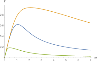
(a)

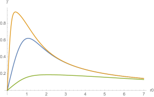
(b)

Figure 4: $T$ as a function of $\hat{r}_{0}$ (left) and $\hat{r}_{0}^{\prime}=\varkappa\,\hat{r}_{0}$ (right) for $\varkappa=5$ (green), $\varkappa=1$ (blue) and $\varkappa=0.2$ (orange).

From the left plot, we can observe that the value $\hat{r}_{0}^{*}$ at which the temperature reaches its maximum value increases with decreasing coupling. In particular, $\hat{r}_{0}^{*}$ diverges as $\varkappa\rightarrow 0$, indicating the Hagedorn regime is reached near infinity in this rescaled variable, as expected.

It is also interesting to understand how the maximum small black string horizon size scales with $g_{6}$. Then, the plot as a function of $\hat{r}_{0}^{\prime}=\varkappa\,\hat{r}_{0}$ (right), so that $r_{0}=\hat{r}_{0}^{\prime}\sqrt{\alpha^{\prime}k}$, is more appropriate. We find that near $\varkappa\approx 0$, $(\hat{r}_{0}^{\prime})_{*}\sim\varkappa^{0.66}$, whereas for very large $\varkappa$, the scaling is $(\hat{r}_{0}^{\prime})_{*}\sim\varkappa^{0.34}$. Consequently, the size of the small, stable black string can be made much larger than that of the AdS₃ throat, by tuning $\varkappa$ to be large. This can be easily achieved for $k>>p$, even if $g_{6}$ small, as required by reliability of the solution. Note this separation of scales is made possible by the existence of an extra parameter, $\varkappa$, with respect to the D3-brane case (which is quite analogous to the self-dual solution with $\varkappa=1$). We would thus expect a clean separation between the Hagedorn regime that is presumably associated with $T_{max}$ and the Cardy one when $\varkappa$ is large.

The scaling of $T_{max}$ with $\varkappa$ is

$$T_{max}\sim\left\{\begin{array}[]{ccc}\frac{1}{2\pi\varkappa\sqrt{\alpha^{\prime}k}}&\;\;\;\mbox{for}&\varkappa>>1\\[5.69054pt] \frac{1}{2\pi\sqrt{\alpha^{\prime}k}}&\;\;\;\mbox{for}&\varkappa<<1\end{array}\right.$$ (4.12)

which interpolates between the LST Hagedorn temperature at small $g_{6}$ and a new, coupling dependent scale that roughly corresponds to $\lambda_{+}-\lambda_{-}$ in (3.20), the coefficient of the operator that turns on the deformation to flat space.

The results of this section suggest that, since large black holes never dominate the thermal ensemble, only the entropy of small black holes can be meaningfully matched to a computation in the holographic dual. It is interesting to compare this to the situation in global AdS₅, where the large black holes are stable, while the small black holes are unstableand never dominate the canonical ensemble.

4.2 Thermodynamics of the non-extremal NCOS $\&$ ODp backgrounds

Let us now add RR flux to this background. In fact, following the steps of section 3, we will start from the S-dual D1-D5 non-extremal solution, perform a TsT transformation and then, eventually, S-dualize again. For simplicity, we set the momentum to zero, though adding it in is straightforward. The NS-NS sector fields read

$$ds^{2}=\frac{\sqrt{f_{1}f_{5}}}{f_{1}f_{5}-\gamma^{2}f}\big{(}d\sigma^{2}-fdt^{2}\big{)}+\sqrt{f_{1}f_{5}}\big{(}\frac{dr^{2}}{f}+r^{2}d\Omega^{2}_{3}\big{)}+\sqrt{\frac{f_{1}}{f_{5}}}\,ds^{2}_{K3}$$ (4.13)

$$B=\frac{\gamma f}{f_{1}f_{5}-\gamma^{2}f}dt\wedge d\sigma\;,\;\;\;\;\;e^{\Phi}=g_{s}\frac{f_{1}}{\sqrt{f_{1}f_{5}-\gamma^{2}f}}$$ (4.14)

while the RR ones are given in the appendix. The functions $f_{1,5}$ and $f$ still take the form (4.2), except that now the expression for the angles is given by

$$r_{1}^{2}:=r_{0}^{2}\sinh 2\alpha_{1}=2\frac{g_{s}\alpha^{\prime}}{v}p\;,\;\;\;\;\;\;r_{5}^{2}:=r_{0}^{2}\sinh 2\alpha_{5}=2\alpha^{\prime}g_{s}k$$ (4.15)

as compared to their expression (4.3) in the NS case. Note that the asymptotic value of the dilaton is $g_{s}/\sqrt{1-\gamma^{2}}$, but we find this parametrisation useful, as $g_{s}$ enters the quantisation condition above.

It is not hard to show that the entropy of this background is identical to that of the undeformed D1-D5 background, which is given by(4.5), upon noting that $g_{s}^{2}\alpha^{\prime 2}/v$ is S-duality invariant. Estimating the energy is somewhat more involved, as in principle it receives contributions not only from the metric, but also the scalars and the two-form gauge fields, including the Chern-Simons terms. We present the details of the computation in appendix C. The end result is remarkably simple

$$M=\frac{Rvr_{0}^{2}}{2\alpha^{\prime 2}g_{s}^{2}}\left[(\cosh 2\alpha_{1}+\cosh 2\alpha_{5})\left(\frac{1}{1-\gamma^{2}}-\gamma B_{\infty}\right)+1+\frac{2}{r_{0}^{2}}\left(\frac{\gamma}{1-\gamma^{2}}-B_{\infty}\right)q_{F_{1}}\right]$$ (4.16)

where $B_{\infty}$ is the value of the $B$ -field at infinity and $q_{F_{1}}$ is the F1 charge (3.40) induced by the constant shifts in the axions. We note that for the particular $B$ - field solution obtained via TsT, its value at infinity is $B_{\infty}=\gamma/(1-\gamma^{2})$, which implies that the axionic terms cancel and the $\gamma$ dependence entirely cancels from the expression for the energy. Thus, in this background, the expression for both the energy and entropy is identical to that in the pure RR non-extremal background, and the $\gamma\rightarrow 1$ limit does not lead to any obvious divergence in the extremal energy.

Let us now review the NCOS decoupling limit of this background. This limit was proposed in [75, 16] for the case of pure non-extremal D5-branes in a background critical $B$-field (obtained by setting $\alpha_{1}=0$, or $f_{1}=1$ in the solution above), and it was shown that the entropy-to-energy relation is Hagedorn in this case. This decoupling limit is non-standard, as it keeps $\alpha_{5}$ finite. According to [16, 75], one should scale

$$\alpha^{\prime}\rightarrow 0\;,\;\;\;\;\;r=\sqrt{\alpha^{\prime}}\,\tilde{r}\;,\;\;\;\;\;r_{0}=\sqrt{\alpha^{\prime}}\,\tilde{r}_{0}\;,\;\;\;\sigma,t=\sqrt{\frac{(1-\gamma^{2})b}{\alpha^{\prime}}}\,\tilde{\sigma},\tilde{t}$$ (4.17)

and the K3 coordinates as $\sqrt{\alpha^{\prime}}$, keeping fixed

$$\ell_{s}^{2}=\frac{g_{s}\alpha^{\prime}}{\sqrt{1-\gamma^{2}}}\;,\;\;\;\;\;b=\frac{\alpha^{\prime}}{\sqrt{1-\gamma^{2}}}\coth\alpha_{5}$$ (4.18)

The ratio of the two fixed scales above defines an effective coupling

$$\tilde{g}=\frac{\ell_{s}^{2}}{b}=g_{s}\tanh\alpha_{5}$$ (4.19)

which is to be held fixed in the decoupling limit. Note that in terms of it, the relation between $\alpha_{5}$ and the quantized NS5 charge becomes

$$\tilde{r}_{0}^{2}\sinh^{2}\alpha_{5}=\tilde{g}k$$ (4.20)

At first sight, one may worry that the explicit factor of $\coth\alpha_{5}$ above effectively makes the scaling of the coordinates energy-dependent. The $\sigma,t$ coordinates can nevertheless be made to scale by a fixed factor of $\epsilon$ if

$$\frac{(1-\gamma^{2})b}{\alpha^{\prime}}=\sqrt{1-\gamma^{2}}\coth\alpha_{5}\equiv\epsilon$$ (4.21)

so one may envisage a state-independent rescaling if one takes the TsT parameter to approach $1$ in an energy-dependent fashion, $\gamma\sim 1-\frac{1}{2}\epsilon^{2}\tanh^{2}\alpha_{5}$, and also $\alpha^{\prime}=\epsilon\,b\tanh^{2}\alpha_{5}$. The fact that $g_{s}$ must depend on the energy as in (4.19) then simply follows from the definition of the fixed scale $\ell_{s}$ in terms of the actual value of the dilaton at infinity. These energy-dependent scalings of $1-\gamma$ and $\alpha^{\prime}$ appear essential for obtaining the desired Hagedorn behaviour.

At the level of the metric, we obtain

$$ds^{2}=\alpha^{\prime}\left[\frac{\sqrt{f_{5}}\tilde{r}^{2}}{\tilde{r}_{0}^{2}\cosh^{2}\alpha_{5}}\cdot\frac{(1-\gamma^{2})b}{\alpha^{\prime 2}}\big{(}d\tilde{\sigma}^{2}-fd\tilde{t}^{2}\big{)}+\sqrt{f_{5}}\big{(}\frac{d\tilde{r}^{2}}{f}+\tilde{r}^{2}d\Omega^{2}_{3}\big{)}+\sqrt{\frac{1}{f_{5}}}\,d\tilde{s}^{2}_{K3}\right]$$ (4.22)

with

$$f_{5}=1+\frac{\tilde{r}_{0}^{2}\sinh^{2}\alpha_{5}}{\tilde{r}^{2}}=1+\frac{\tilde{g}k}{\tilde{r}^{2}}\;,\;\;\;\;\;f=1-\frac{\tilde{r}_{0}^{2}}{\tilde{r}^{2}}$$ (4.23)

Using (4.18) and (4.20), the prefactor of the first term becomes $\sqrt{f_{5}\,}\tilde{r}^{2}/(\tilde{g}kb)$, so the $\alpha_{5}$ dependence entirely drops out. Taking into account the rescaling (4.17) of the spacetime coordinates, which imply

$$R=\sqrt{\frac{(1-\gamma^{2})b}{\alpha^{\prime}}}\,\tilde{R}\;,\;\;\;\;\;\tilde{E}=\sqrt{\frac{(1-\gamma^{2})b}{\alpha^{\prime}}}\,E$$ (4.24)

the total energy and entropy of this system become

$$\tilde{M}=\frac{\tilde{R}v\tilde{r}_{0}^{2}}{2b\tilde{g}^{2}}(2+\cosh 2\alpha_{5})\;,\;\;\;\;\;S=\frac{2\pi\tilde{R}v\tilde{r}_{0}^{3}\sinh\alpha_{5}}{\tilde{g}^{2}\sqrt{b}}=\frac{2\pi\tilde{R}v\tilde{r}_{0}^{2}}{\tilde{g}^{2}}\sqrt{\frac{\tilde{g}k}{b}}$$ (4.25)

Thanks to the modified quantisation condition (4.20), the energy above extremality is simply

$$\tilde{E}=\frac{3\tilde{R}v\tilde{r}_{0}^{2}}{2b\tilde{g}^{2}}$$ (4.26)

and thus the entropy-to-energy relation is pure Hagedorn

$$S=\frac{4\pi}{3}\tilde{E}\sqrt{\tilde{g}kb}$$ (4.27)

The Hagedorn temperature is set by $\tilde{g}b$, which is precisely the expected LST tension.

This concludes our review of the pure non-extremal D5 NCOS limit. Now, we would like to add D1 branes to the picture. To make sure that the irrelevant deformation associated to pure LST is turned off, we set $v$ to its attractor value, $p/k$. Then, $\alpha_{1}=\alpha_{5}=\alpha$. Taking the same limit as before, the analysis is almost identical, only the entropy differs by a factor of $\cosh\alpha$. Remarkably, the energy above extremality is still given by (4.26), despite the fact that the total ADM mass is changed. The final answer we obtain for the entropy is

$$S=\frac{2\pi\tilde{R}v\tilde{r}_{0}^{2}}{\tilde{g}^{2}}\sqrt{\frac{\tilde{g}k}{b}\left(1+\frac{\tilde{g}k}{\tilde{r}_{0}^{2}}\right)}=2\pi\sqrt{\frac{2}{3}pk\,\tilde{E}\tilde{R}+\frac{4}{9}\tilde{g}kb\tilde{E}^{2}}$$ (4.28)

We immediately note that the high-energy behaviour remains Hagedorn, but we find, in addition, Cardy behaviour at lower energies, as expected from the fact that the system now flows to a CFT in the IR. This matches the form of a single-trace $T\bar{T}$ - deformed CFT, including the particular dependence on $p$ and $k$. However, the numerical coefficient of the Cardy term clearly does not match the one in the IR. This is puzzling, given that the solution (4.22) does reduce to standard AdS${}_{3}\times S^{3}$ in the IR limit, $b\rightarrow 0$ with $\tilde{r}/\sqrt{b}$ and $\tilde{r}_{0}/\sqrt{b}$ fixed. This can be traced back to the definition of the energy above extremality (4.26) which does not agree, in the AdS decoupling limit, with its standard decoupled counterpart. One possible way to circumvent this problem would be to adjust the finite part of the $B$ - field at infinity so that the first term in (4.16) entirely drops out; then the energy above extremality differs by a factor of $3$ from (4.26), and the entropy-to-energy relation becomes

$$S=2\pi\sqrt{2pk\,\tilde{E}^{\prime}\tilde{R}+4\tilde{g}kb\tilde{E}^{\prime 2}}$$ (4.29)

This scales in the same way as the LST entropy.

Note that we have assumed the same decoupling limit for the D1-D5 system as for the pure D5 one. While the entropy argument goes through and gives the expected structure, one should also check the effect of the limit on the spacetime metric. The only interesting factor is the coefficient of the $-\delta\tilde{t}^{2}+d\tilde{\sigma}^{2}$ term which, after pulling out an overall factor of $\alpha^{\prime}$, reads

$$\frac{(1-\gamma^{2})b}{\alpha^{\prime 2}}\cdot\frac{\tilde{r}^{2}}{\tilde{r}_{0}^{2}(1+2\sinh^{2}\alpha)+\tilde{r}_{0}^{4}\sinh^{4}\alpha/\tilde{r}^{2}}$$ (4.30)

Replacing the prefactor by its value (4.21) and using (4.20), it is clear that $\alpha$ no longer drops out from the metric. This is not a priori problematic, as one does, in general, expect the metric to non-trivially depend on the energy of the solution. The fact that the asymptotic metric depends on it is somewhat less desirable, but can happen for more general boundary conditions at infinity.

Letting $\alpha_{1}\neq\alpha_{5}$ one could in principle understand if and how the thermodynamics depends on the coupling constant in the system, namely $v/v_{*}$. The same computation can be reproduced in the OD$1$ theory, by working in terms of the S-dual variables.

4.3 Three-dimensional truncation of the self-dual black string

Even though this article is mostly concerned with the decoupled asymptotic linear-dilaton-like black string backgrounds, it is interesting, for comparison, to also study the asymptotically flat six-dimensional backgrounds from the same perspective. We have already drawn a parallel between the entropies of black holes in these spacetimes in section 4.1. Next, we would like to compare the asymptotic symmetries of the ALD and the asymptotically flat black string spacetimes.

The asymptotic symmetries of the (pure NS) linear dilaton background were analysed in detail in [45]. Since the dual LST theory lives only along the black string directions ($\sigma,t$ and the internal manifold) it is justified in this case, in order to understand the “spacetime” symmetries of the dual field theory, to only concentrate on the $\sigma,t$ dependence of the asymptotic symmetry generators, ignoring their dependence on the $S^{3}$ factor, associated to the R-symmetry directions. To simplify the analysis, [45] thus used a spherically-symmetric consistent truncation to three dimensions, containing only the $3d$ metric and the dilaton. Also, they made central use of the known black hole solutions in the ALD background, as the asymptotic symmetry generators were fixed by requiring that their symplectic product with the metric perturbations that simply changed the black hole parameters vanish. Interestingly, [45] found that the asymptotic symmetry generators are precisely the field-dependent generalisation of two-dimensional conformal transformations that appears in single-trace $T\bar{T}$ - deformed CFTs, and the non-trivial symmetry algebra matched exactly to the order it was computed.

We would now like to study the asymptotic symmetries of the asymptotically flat black string backgrounds from the same viewpoint, which focuses on the dependence of the asymptotic symmetry generators on $\sigma,t$ and ignores to first approximation the $S^{3}$ dependence. In this section, we prepare the ground for this computation, by writing down a simple, spherically symmetric consistent truncation of these backgrounds, and describing the black string solutions from this three-dimensional point of view.

We concentrate on the simplest asymptotically flat background, which has self-dual pure $H_{3}$ flux and is given in (3.9). The dilaton is a constant. Since, as explained, we are less interested in what happens on the $S^{3}$, we will concentrate on the following consistent truncation of the six-dimensional theory to three dimensions, which only keeps the spherically symmetric modes

$$ds_{6}^{2}=e^{-6F}ds_{3}^{2}+e^{2F}d\Omega_{3}^{2}\;,\;\;\;\;\;H=2k\alpha^{\prime}(\omega_{S^{3}}+\star_{6}\omega_{S^{3}})=\star H\;,\;\;\;e^{2\phi}=\frac{k}{p}=const$$ (4.31)

where $ds_{6}^{2}$ is the six-dimensional string frame metric, $d\Omega_{3}^{2},\omega_{S^{3}}$ are the metric and volume form on the unit three sphere (they are given explicitly in (A.8),(A.7)), and $F$ only depends on the three-dimensional coordinates. The fact that the six-dimensional dilaton is constant implies that its value at infinity equals its attractor value, $g_{6}^{2}=k/p$. The normalisation of the three-dimensional Einstein metric was chosen so it be in Einstein frame. The six-dimensional equations of motion are

$$R_{MN}+2\nabla_{M}\nabla_{N}\phi=\frac{1}{4}H_{MPQ}H_{N}{}^{PQ}\;,\;\;\;\;\Box\phi-2(\partial\phi)^{2}=-\frac{1}{12}H^{2}\;,\;\;\;\;\;d(e^{-2\phi}\star H)=0$$ (4.32)

The last two of them are trivially satisfied by our Ansatz (as $H^{2}=H\wedge\star H=H\wedge H=0$), while the spherical and non-compact $3d$ components of the Einstein equations lead to the following constraints on the scalar field $F$ and the $3d$ Einstein frame metric

$$\Box F=2e^{-8F}-\frac{a^{2}}{2}\,e^{-12F}\;,\;\;\;\;\;\;G_{\mu\nu}=12\partial_{\mu}F\partial_{\nu}F-6g_{\mu\nu}(\partial F)^{2}+g_{\mu\nu}\left(3e^{-8F}-\frac{a^{2}}{2}e^{-12F}\right)$$ (4.33)

with $a=2k\alpha^{\prime}$, which can be easily derived from the three-dimensional action

$$S=\int d^{3}x\sqrt{g}\left(R-12(\partial F)^{2}+6e^{-8F}-a^{2}e^{-12F}\right)$$ (4.34)

Let us now try to understand how the NS5-F1 solution (4.1) fits into this. One immediately reads off

$$e^{2F}=f_{5}r^{2}=r_{5}^{2}+r^{2}\;,\;\;\;\;\;r_{5}^{2}(r_{0}^{2}+r_{5}^{2})=(\alpha^{\prime}k)^{2}$$ (4.35)

where $r_{5}^{2}=r_{0}^{2}\sinh^{2}\alpha_{5}$. The scalar $F$ diverges logarithmically in this limit; note, however, that its potential is well-behaved. The $6d$ dilaton is

$$e^{2\phi}=g_{6}^{2}\frac{f_{5}}{f_{1}}=\frac{k}{p}\;\;\;\;\Rightarrow\;\;\;\;f_{1}=f_{5}\;,\;g_{6}^{2}=\frac{k}{p}$$ (4.36)

The three-dimensional Einstein frame metric reads

$$ds_{3}^{2}=f_{5}^{2}r^{6}\left[-dt^{2}+d\sigma^{2}+\frac{r_{0}^{2}}{r^{2}}\left(\cosh\alpha_{n}dt+\sinh\alpha_{n}d\sigma\right)^{2}\right]+\frac{f_{5}^{4}r^{6}}{f}dr^{2}$$ (4.37)

with $f,\alpha_{n}$ given in (4.2), (4.3). The asymptotics of the Einstein frame are conformally flat.

Let us now study the black hole solutions in this background. Following [45], it is convenient to rescale the coordinates as

$$r=g_{6}\alpha^{\prime}\tilde{r}\;,\;\;\;\;\;r_{0}=g_{6}\alpha^{\prime}\tilde{r}_{0}$$ (4.38)

and introduce the parametrization

$$\tilde{r}=\rho+\frac{\tilde{r}_{0}^{2}}{4\rho}\;,\;\;\;\;\;\;\;L_{u,v}=\frac{\tilde{r}_{0}^{2}e^{\pm 2\alpha_{n}}}{4}\;,\;\;\;\;\;\;U,V=\sigma\pm t$$ (4.39)

Then

$$e^{2F}=r^{2}+r_{5}^{2}=(g_{6}\alpha^{\prime})^{2}\left(\rho^{2}+\frac{\tilde{r}_{0}^{2}}{2}\cosh 2\alpha_{5}+\frac{\tilde{r}_{0}^{4}}{16\rho^{2}}\right)\equiv(g_{6}\alpha^{\prime})^{2}e^{2\tilde{F}}$$ (4.40)

where

$$e^{2\tilde{F}}=\rho^{2}+\sqrt{4L_{u}L_{v}+\frac{k^{2}}{(g_{6}^{2}\alpha^{\prime})^{2}}}+\frac{L_{u}L_{v}}{\rho^{2}}=\rho^{2}+\sqrt{4L_{u}L_{v}+\frac{p^{2}}{\alpha^{\prime 2}}}+\frac{L_{u}L_{v}}{\rho^{2}}$$ (4.41)

The metric can be written as

$$ds^{2}=(g_{6}\alpha^{\prime})^{6}e^{4\tilde{F}}\left[\rho^{2}dUdV+L_{u}dU^{2}+L_{v}dV^{2}+\frac{L_{u}L_{v}}{\rho^{2}}\,dUdV\right]+(g_{6}\alpha^{\prime})^{8}e^{8\tilde{F}}\,\frac{d\rho^{2}}{\rho^{2}}$$ (4.42)

which is extremely similar to the ALD metric of [45] in the same parametrization. The quantities $L_{u,v}$ are related to the energy above extremality (4.6) and angular momenta of the black holes as

$$E=R\left(L_{u}+L_{v}-\frac{2p}{\alpha^{\prime}}+2\sqrt{4L_{u}L_{v}+\frac{p^{2}}{\alpha^{\prime 2}}}\right)$$ (4.43)

where we used the fact that $g_{6}^{2}=k/p$, implying that $\alpha_{1}=\alpha_{5}$. This highly resembles the formula in [45], up to the factor of $2$, which reflects the different scaling of $\alpha_{5}$. The momentum is simply

$$P=\frac{n}{R}=\frac{Rvr_{0}^{2}\sinh 2\alpha_{n}}{2g_{s}^{2}\alpha^{\prime 2}}=R(L_{u}-L_{v})$$ (4.44)

We will now use this parametrisation of the black string solutions to work out the asymptotic symmetries of this spacetime, in order to facilitate the comparison with the corresponding formulae in the ALD case.

4.4 Asymptotic symmetries of the self-dual black holes

We would now like to find the asymptotic symmetries of the self-dual black holes within this truncation. Since we do not know, a priori, which boundary conditions to impose, we will be following the same strategy that we used in [45] to find the asymptotic symmetries of the ALD background, namely to require that the asymptotic symmetry generators have zero symplectic product with the metric and scalar field perturbations that simply change the mass and angular momentum parameters of the black holes - namely, the parameters $L_{u,v}$ in the solutions above - as the latter should clearly be allowed perturbations of the spacetime.

To find the asymptotic symmetries, we first choose a gauge that fixes the radial dependence of the diffeomorphism. We will thus be working in radial gauge

$$(\mathcal{L}_{\xi}g)_{\rho\mu} =0$$ (4.45)

The resulting gauge-fixed diffeomorphism takes the form

$$\xi =\frac{\rho^{5}}{(\rho^{4}+\rho^{2}\beta/\alpha^{\prime}+L_{u}L_{v})^{2}}F_{\rho}(U,V)\partial_{\rho}+\bigg{(}F_{U}(U,V)+\frac{(\alpha^{\prime}g_{6})^{2}(\rho^{2}\partial_{v}F_{\rho}-L_{v}\partial_{u}F_{\rho})}{\rho^{4}-L_{u}L_{v}}\bigg{)}\partial_{U}+$$

$$\;\;\;\;+\,\bigg{(}F_{V}(U,V)+\frac{(\alpha^{\prime}g_{6})^{2}(\rho^{2}\partial_{u}F_{\rho}-L_{u}\partial_{v}F_{\rho})}{\rho^{4}-L_{u}L_{v}}\bigg{)}\partial_{V}$$ (4.46)

where we introduced the notation $\beta=\sqrt{p^{2}+4\alpha^{\prime 2}L_{u}L_{v}}$ . This is very similar to the corresponding radial diffeomorphism in the ALD spacetime, except for the fall-off of the radial component.

The symplectic form receives contributions from both the metric and the scalar

$$\omega=\frac{1}{16\pi G_{3}}(\omega_{g}+\omega_{sc})$$ (4.47)

For an action of the form (4.34), the general expressions for these contributions, for two arbitrary variations $\delta_{1},\delta_{2}$ of the fields are [80]

$$\omega^{\mu}_{g}=\frac{1}{2}\bigg{(}(2\nabla_{\lambda}h_{1\rho}^{\mu}-\nabla^{\mu}h_{1\lambda\rho})h_{2}^{\lambda\rho}-\nabla_{\rho}h_{1}h_{2}^{\rho\mu}+h_{1}(\nabla_{\rho}h_{2}^{\rho\mu}-\nabla^{\mu}h_{2})-(1\leftrightarrow 2)\bigg{)}$$ (4.48)

$$\omega^{\mu}_{sc}=\frac{\kappa}{2}\bigg{(}-\delta_{1}(\nabla^{\mu}F)\delta_{2}F-\frac{1}{2}h_{1}\nabla^{\mu}F\delta_{2}F-(1\leftrightarrow 2)\bigg{)}$$ (4.49)

where $\kappa/2$ is the coefficient of the scalar kinetic term in the action ($\kappa=24$ in our case) and we use the notation $h^{i}_{\mu\nu}=\delta_{i}g_{\mu\nu}$ and $h_{i}=g^{\mu\nu}\delta_{i}g_{\mu\nu}$. The falloff conditions on the symplectic form that ensure it is conserved and normalisable are, in our coordinates

$$\omega_{UV}=o(\rho^{0})\hskip 28.45274pt\omega_{\rho U,\rho V}=o(\rho^{-1})$$ (4.50)

where $\omega_{\mu\nu}=\epsilon_{\mu\nu\alpha}\omega^{\alpha}$ and the notation $o(\rho^{a})$ signifies that the falloff needs to be faster than $\rho^{a}$. We evaluate the symplectic form on a perturbation that simply changes the black hole parameters

$$\delta_{1}=\delta L_{u}\frac{\partial}{\partial L_{u}}+\delta L_{v}\frac{\partial}{\partial L_{v}}$$ (4.51)

and one that corresponds to the action of a diffeomorphism of the form (4.46), $\delta_{2}=\mathcal{L}_{\xi}$.

Requiring that the coefficients of $\delta L_{u},\delta L_{v}$ vanish independently, the asymptotic falloff condition on $\omega_{UV}$ translates into the following two constraints

$$\partial_{U}F_{U}+\partial_{V}F_{V} =\frac{\beta}{2\alpha^{\prime}L_{v}}\partial_{V}F_{U}=\frac{\beta}{2\alpha^{\prime}L_{u}}\partial_{U}F_{V}$$ (4.52)

These equations, up to a factor of 2 difference, are the same as in the ALD background. The solutions to the equations are given in terms of two arbitrary functions $f,\bar{f}$

$$F_{U}(U,V)=f(u)+\frac{\beta-\tilde{\beta}}{4\alpha^{\prime}L_{u}}\bar{f}(v)\hskip 28.45274ptF_{V}(U,V)=\bar{f}(v)+\frac{\beta-\tilde{\beta}}{4\alpha^{\prime}L_{v}}f(u)$$ (4.53)

of the following field-dependent coordinates:

$$u=U+\frac{4\alpha^{\prime}L_{v}}{\beta+\tilde{\beta}}\,V\hskip 28.45274ptv=V+\frac{4\alpha^{\prime}L_{u}}{\beta+\tilde{\beta}}\,U$$ (4.54)

where we have introduced the notation

$$\tilde{\beta}=\sqrt{p^{2}-12\alpha^{\prime 2}L_{u}L_{v}}$$ (4.55)

The field-dependent coordinates (4.54) reduce to $U$ and, respectively, $V$ in the $L_{u},L_{v}\rightarrow 0$ or $\alpha^{\prime}\rightarrow 0$ limit, while $F_{U,V}$ become purely holomorphic functions of these fixed coordinates. Another interesting fact to note is that the expression for $\tilde{\beta}$ breaks down at an energy or, correspondingly, horizon radius that precisely coincides with the maximum value of the radius of the small black strings we discussed in section 4.1

$$(L_{u}L_{v})_{*}=\frac{(\tilde{r}_{0}^{*})^{4}}{16}=\frac{p^{2}(\hat{r}_{0}^{*})^{4}}{16\alpha^{\prime 2}}=\frac{p^{2}}{12\alpha^{\prime 2}}$$ (4.56)

where $\hat{r}_{0}^{*}=\sqrt[4]{\frac{4}{3}}$ is the value of the rescaled radius that corresponds to $T_{max}$ for $\varkappa=1$.

The $\omega_{\rho U,\rho V}$ components of the symplectic form contain terms that behave have both as $\rho$ and $\frac{1}{\rho}$ at infinity. However, these terms are total derivatives, in the sense that $\omega_{\rho\sigma}=\partial_{\sigma}(...)$, which vanishes upon integration on the $\sigma$ circle. The radial function $F_{\rho}$ is not fixed by these constraints but, just like in the ALD background, it is fixed by the symplectic form evaluated on variations generated by two different diffeomorphisms of the form above, which yield the constraint

$$L_{u}\partial^{2}_{V}F_{\rho}+L_{v}\partial^{2}_{U}F_{\rho}=\frac{\beta}{2\;\alpha^{\prime}}\partial_{U}\partial_{V}F_{\rho}$$ (4.57)

The solution to this equation takes the general form

$$F_{\rho}(U,V) =f_{\rho}(u)+\bar{f}_{\rho}(v)$$ (4.58)

for two new functions of the field-dependent coordinates.

We would now like to compute the charges associated to these asymptotic diffeomorphisms and show they are non-vanishing. Since our background depends on constant parameters, the only nontrivial charges will correspond to the energy and momentum, already computed in (4.43), (4.44). To obtain non-trivial charges associated with the general functions $f,\bar{f}$ in (4.53), we first perturb the background using an allowed diffeomorphism, denoted $\eta$ and parametrized by $h(u),\bar{h}(v),h_{\rho}(u),\bar{h}_{\rho}(v)$, and then compute the charge difference associated to another asymptotic diffeomorphism, $\xi$, parametrized by $f(u),\bar{f}(v),f_{\rho}(u),\bar{f}_{\rho}(v)$. The result takes the form

$$\delta_{\eta}Q_{\xi} =\frac{g_{6}^{2}\alpha^{\prime 2}}{4\pi G_{3}}\frac{\tilde{\beta}}{\beta+\tilde{\beta}}\oint d\sigma\bigg{[}r_{u}\bigg{(}2L_{u}f(u)h^{\prime}(u)+g_{6}^{2}\alpha^{\prime 2}(f(u)h^{\prime\prime}_{\rho}(u)-h(u)f^{\prime\prime}_{\rho}(u))\bigg{)}-$$

$$-r_{v}\bigg{(}2L_{v}\bar{f}(v)\bar{h}^{\prime}(v)+g_{6}^{2}\alpha^{\prime 2}(\bar{f}(v)\bar{h}^{\prime\prime}_{\rho}(v)-\bar{h}(v)\bar{f}^{\prime\prime}_{\rho}(v))\bigg{)}+$$

$$+\frac{1}{2}\bigg{(}r_{u}f^{\prime}_{\rho}(u)\bar{h}^{\prime}(v)+r_{v}f_{\rho}(u)\bar{h}^{\prime\prime}(v)-r_{v}\bar{f}^{\prime}_{\rho}(v)h^{\prime}(u)-r_{u}\bar{f}_{\rho}(v)h^{\prime\prime}(u)\bigg{)}\bigg{]}$$ (4.59)

where $r_{u,v}$ are the normalised radii of the field-dependent coordinates (4.54)

$$r_{u}:=\partial_{\sigma}u=\frac{4\alpha^{\prime}L_{v}+\beta+\tilde{\beta}}{\beta+\tilde{\beta}}\hskip 56.9055ptr_{v}:=\partial_{\sigma}v=\frac{4\alpha^{\prime}L_{u}+\beta+\tilde{\beta}}{\beta+\tilde{\beta}}$$ (4.60)

It is clear that the last line vanishes after integration by parts. We are left with the following result

$$\delta_{\eta}Q_{\xi} =\frac{g_{6}^{2}\alpha^{\prime 2}}{4\pi G_{3}}\frac{\tilde{\beta}}{\beta+\tilde{\beta}}\oint d\sigma\;r_{u}\bigg{(}2L_{u}f(u)h^{\prime}(u)+g_{6}^{2}\alpha^{\prime 2}(f(u)h^{\prime\prime}_{\rho}(u)-h(u)f^{\prime\prime}_{\rho}(u))\bigg{)}+RM$$ (4.61)

where ‘RM’ stands for the expression obtained by replacing $f,h$ etc. by $\bar{f},\bar{h}$ and $u\rightarrow v$. This result is extremely similar with the analogous expression in the ALD spacetime. Setting, for simplicity, the radial piece of the diffeomorphism to zero, the difference simply amounts to replacing $\tilde{\beta}$ by $p$ (the same holds at the level of the field-dependent coordinates), which becomes negligible at low energies.

To conclude, it is rather remarkable that i) the asymptotic symmetries that we have obtained in this simple manner are so similar to the symmetries of single-trace $T\bar{T}$ (identified with the asymptotic symmetries of the ALD spacetime) and ii) they appear to know about the termodynamic stability of the backgrounds that they depend on, in the sense that the symmetry generators become imaginary precisely when one reaches the large, unstable black string region. It would be very interesting to better understand this connection between asymptotically flat backgrounds and $T\bar{T}$.

5 Discussion

In this article, we have argued that turning on a particular $21$-dimensional subset of the $22$ maximally supersymmetric single-trace irrelevant deformations of the D1-D5 CFT for a finite amount leads to a UV-complete theory decoupled from gravity, which is in general a deformation of little string theory, compactified on K3. Our argument was largely based on the supergravity description of these deformations, which are characterised by the degeneration of the flat asymptotia to linear dilaton-like ones in specific ways that we could identify with known decoupling limits of string theory. By studying the behaviour of entropy in these theories, inferred from that of the dual black holes, we also argued that the resulting two-dimensional theories should admit a $T\bar{T}$ - like effective description. Finally, we put forth evidence that, for low enough energies, the asymptotically flat black strings, too, admit a similar description, as suggested by the resemblance between the asymptotic symmetry generators we found for flat space and the field-dependent coordinate transformations characteristic of $T\bar{T}$.

If this global picture is correct, there are many interesting future directions to explore.

One such direction is to gain a better technical understanding of the general ALD-like spacetimes we discussed and their associated holographic dictionary. One may, for example, study the asymptotic symmetries of the general such spacetimes and check whether they, too, display $T\bar{T}$ - like features. Another interesting question is whether the behaviour of the entropy and symmetries changes if several $\lambda_{\bar{\imath}}$ deformations are turned on at the same time. One may also try to understand the precise map between supergravity modes and their dual operators, by adapting the holographic renormalisation technique to this setup (see [81] for some early work); the careful linearised analysis of the fields in a consistent truncation of the standard ALD background, performed in [45], already showed several unusual features. It is also interesting to understand how the matching of supersymmetry multiplets works in these cases; for example, whether fields in the same multiplet acquire the same momentum-dependence in their radial fall-offs.

All these analyses would presumably provide important clues for what the properties of the dual theories should be and, in particular, which observables should be expected to be universal. In addition, this could prove to be a useful warm-up exercise for flat space holography, with which it shares many features [82], but without some of the puzzles related to decoupling and the black hole instability.

Another possibility is to approach the same problem from the field-theory perspective, using conformal perturbation theory and/or supersymmetry. One may hope, for example, that for the case of the $SO(21)$ - singlet irrelevant deformation, its mixing with other operators may be constrained enough to yield the deformation solvable. The conformal perturbation theory calculation may be performed at a generic point in moduli space, or at the orbifold point. In the latter case, it may be possible to understand the exact single-trace $T\bar{T}$ deformation in terms of the dual worldsheet theory and, to the extent this field progresses [83], study the other types of deformations by turning on RR fields in the bulk.

Still from the boundary perspective, it would be very interesting to further explore the properties of non-commutative open string theories and, in particular, understand the assumptions that underlie the particular energy dependence of the five-dimensional NCOS decoupling parameters, which is ultimately responsible for the observed Hagedorn behaviour in the supergravity dual. It would of course be interesting if this could be further extended to general OD$p$ theories.

Finally, it would be interesting to see if the perspective of section 4 can shed light on more general black holes, such as Reissner-Nordström or Kerr ones.

Acknowledgements

We are grateful to Iosif Bena, Nikolay Bobev, Soumangsu Chakraborty, Ruben Minasian and especially Kyriakos Papadodimas for insightful conversations. The work of NK is supported by the ERC Consolidator Grant 772408-Stringlandscape. The work of SG is supported by the ERC Starting Grant 853507. SG and NK also thank CERN and EPFL, where part of this work was carried out, for their hospitality.

Appendix A Details of the six-dimensional supersymmetric solutions

In this appendix, we fill in many of the details of the supersymmetric solutions discussed in section 2, including conventions and the explicit form of the Killing spinors.

A.1 Supersymmetry conventions

In six dimensions, the R-symmetry group is USp$(2)$ for $\mathcal{N}=(1,0)$ supergravity and USp$(4)$ for $\mathcal{N}=(2,0)$. These groups are isomorphic to spin groups [59]

$$\text{USp}(2)\cong SU(2)\cong Spin(3)$$

$$\text{USp}(4)\cong Spin(5)$$ (A.1)

and we can construct their generators in the standard way using gamma matrices in three and, respectively, five Euclidean dimensions. In $\mathcal{N}=(1,0)$ supergravity, the spinors are USp$(2)$ doublets of six-dimensional Weyl spinors satisfying the symplectic Majorana condition; in $\mathcal{N}=(2,0)$, they are quadruplets of six-dimensional Weyl spinors that transform under USp$(4)$ and satisfy the corresponding symplectic Majorana condition.

In the following, $\mu,\nu$ will denote curved spacetime indices, and $a,b$ will be six-dimensional tangent space indices. In $\mathcal{N}=(1,0)$ theories, the $USp(2)$ structure is trivial, as all bosonic quantities are singlets under it, and all fermionic ones are doublets; we will consequently drop all associated indices. In $\mathcal{N}=(2,0)$ theories, given the correspondence between the fundamental and, respectively, traceless antisymmetric representation of $USp(4)$ and the spinor and, respectively, vector representation of $Spin(5)$, we will be using $Spin(5)$ spinor indices $A,B=\{1,\ldots,4\}$ on the fermions, and vector indices $i,j=\{1,\ldots 5\}$ on the bosons. Meanwhile, the indices $\bar{\imath},\bar{\jmath}=\{1,\ldots Q\}$ transform in the vector representation of $SO(Q)$. We will be using the notation $\gamma^{a}$ for the six-dimensional Lorentzian gamma matrices, and $\Gamma^{i}$ for the five-dimensional Euclidean gamma matrices. The chirality matrix in six dimensions is defined as

$$\gamma_{7} =-\gamma^{0}...\gamma^{5}$$ (A.2)

and the chirality projectors are given by $P_{\pm}=\frac{I_{7}\pm\gamma_{7}}{2}$. The left and right spinors satisfy $P_{+}\varepsilon_{+}=\varepsilon_{+}$ and $P_{-}\varepsilon_{-}=\varepsilon_{-}$, respectively.

In $\mathcal{N}=(2,0)$ theories, the supersymmetry variations are given by

$$\delta\psi_{\mu A} =\nabla_{\mu}\varepsilon_{A}+\frac{1}{4}F_{\mu ab}^{+i}\gamma^{a}\gamma^{b}(\Gamma^{i})_{A}^{\;B}\varepsilon_{B}$$ (A.3)

$$\delta\chi^{\bar{\imath}}_{A} =\frac{1}{\sqrt{2}}\gamma^{\mu}P_{\mu}^{i\bar{\imath}}(\Gamma^{i})_{A}^{\;B}\varepsilon_{B}-\frac{1}{12}\gamma^{\mu}\gamma^{\nu}\gamma^{\rho}F^{-\bar{\imath}}_{\mu\nu\rho}\varepsilon_{A}$$ (A.4)

where the covariant derivative contains both the spacetime spin connection, $\omega_{\mu}{}^{ab}$, and the $SO(P)$ one, $Q_{\mu}^{ij}$

$$\nabla_{\mu}\varepsilon_{A}=\bigg{(}\partial_{\mu}+\frac{1}{4}\omega_{\mu}^{\;ab}\gamma_{a}\gamma_{b}\bigg{)}\varepsilon_{A}-\frac{1}{4}Q_{\mu ij}(\Gamma^{i}\Gamma^{j})_{A}^{\;B}\varepsilon_{B}$$ (A.5)

whose construction in terms of the decomposition of the Lie algebra element $dg\,g^{-1}$ was explained in section 2 and is given by

$$Q^{ij}=(dgg^{-1})^{ij}=-X^{i\Lambda}dX^{j}_{\Lambda}\;,\;\;\;\;\;\;Q^{\bar{\imath}\bar{\jmath}}=(dgg^{-1})^{\bar{\imath}\bar{\jmath}}=X^{\bar{\imath}\Lambda}dX^{\bar{\jmath}}_{\Lambda}$$ (A.6)

We have also included the $SO(Q)$ connection, for completeness. In $\mathcal{N}=(1,0)$ theories, there is only one self-dual form, and so the index $i$ takes a single value. Consequently, $Q=0$, case in which the equations simplify to (2.16).

A.2 Details of the computation of the $(1,0)$ solutions

In the $\mathcal{N}=(1,0)$ case, we can replace the doublet of spinors satisfying the Majorana condition by a single unconstrained spinor. Let us now explicitly solve the Killing spinor equations (2.16) in the $(1,0)$ theory. Our derivation closely follows that of [61, 60] for $\mathcal{N}=(2,0)$. We choose (Hopf) coordinates on the sphere, denoted $\{\psi,\theta,\varphi\}$

$$d\Omega^{2}_{3} =\frac{1}{4}(d\theta^{2}+d\psi^{2}+d\varphi^{2}+2\cos\theta d\varphi d\psi)$$ (A.7)

The orientation on $S^{3}$ is

$$\omega_{S^{3}}=\frac{\sin\theta}{8}d\psi\wedge d\theta\wedge d\varphi$$ (A.8)

and use the convention $\epsilon_{r\sigma t\psi\theta\varphi}=+\sqrt{g}$ when computing the Hodge dual. The vielbein associated to the metric (2.17) is given by

$$e^{0}=e^{U}dt\;,\hskip 8.5359pte^{1}=e^{U}d\sigma\;,\hskip 8.5359pte^{2}=e^{-U}dr\;,\hskip 8.5359pte^{3}=\frac{r\,e^{-U}}{2}(d\psi+\cos\theta d\varphi)$$ (A.9)

$$e^{4}=\frac{r\,e^{-U}}{2}d\theta\;,\hskip 8.5359pte^{5}=\frac{r\,e^{-U}}{2}\sin\theta d\varphi$$ (A.10)

and the nonzero components of the spin connection $\omega_{\mu}^{\;ab}=e^{\;a}_{\nu}\nabla_{\mu}e^{\;\nu b}$ are

$$\omega_{02} =e^{U}U^{\prime}e^{0}\;,\hskip 14.22636pt\omega_{12}=-e^{U}U^{\prime}e^{1}\;,\hskip 14.22636pt\omega_{23}=\frac{e^{U}(1-rU^{\prime})}{r}e^{3}\;,\hskip 14.22636pt\omega_{24}=\frac{e^{U}(1-rU^{\prime})}{r}e^{4}$$ (A.11)

$$\omega_{25} =\frac{e^{U}(1-rU^{\prime})}{r}e^{5}\;,\hskip 14.22636pt\omega_{34}=\frac{e^{U}}{r}e^{5}\;,\hskip 14.22636pt\omega_{35}=-\frac{e^{U}}{r}e^{4}\;,\hskip 14.22636pt\omega_{45}=\frac{e^{U}}{r}(-e^{3}+2\cot\theta e^{5})$$ (A.12)

where $U^{\prime}=\partial_{r}U$. In terms of the vielbeine, our Ansatz (2.19) for the 3-forms is given by

$$H^{+} =\frac{Ze^{3U}}{r^{3}}\big{(}e^{3}\wedge e^{4}\wedge e^{5}-e^{0}\wedge e^{1}\wedge e^{2}\big{)}$$ (A.13)

$$H^{-\bar{\imath}} =\frac{Z^{\bar{\imath}}e^{3U}}{r^{3}}\big{(}e^{3}\wedge e^{4}\wedge e^{5}+e^{0}\wedge e^{1}\wedge e^{2}\big{)}$$ (A.14)

Plugging this into the tensorino equations (A.4) and using the chirality of the $6d$ spinor they can be reduced to

$$\frac{1}{\sqrt{2}}\gamma^{2}e_{2}^{r}P^{\bar{\imath}}_{r}\varepsilon-\frac{Z^{\bar{\imath}}e^{3U}}{r^{3}}\gamma^{0}\gamma^{1}\gamma^{2}\varepsilon=0$$ (A.15)

As explained in the main text, for $Z_{\bar{\imath}}\neq 0$ this leads to the projection

$$\gamma^{0}\gamma^{1}\varepsilon=\varepsilon$$ (A.16)

as well as the equation (2.37) for $P_{r}^{\bar{\imath}}$.

Let us now turn to the gravitino equations. Writing them explicitly in components, they read

$$e^{-U}\partial_{t}\varepsilon+\frac{1}{2}e^{U}U^{\prime}\gamma^{0}\gamma^{2}\varepsilon-\frac{1}{2}\frac{Ze^{3U}}{r^{3}}\gamma^{1}\gamma^{2}\varepsilon=0$$ (A.17)

$$e^{-U}\partial_{\sigma}\varepsilon+\frac{1}{2}e^{U}U^{\prime}\gamma^{2}\gamma^{1}\varepsilon-\frac{1}{2}\frac{Ze^{3U}}{r^{3}}\gamma^{2}\gamma^{0}\varepsilon=0$$ (A.18)

$$e^{U}\partial_{r}\varepsilon-\frac{1}{2}\frac{Ze^{3U}}{r^{3}}\gamma^{0}\gamma^{1}\varepsilon=0$$ (A.19)

$$\frac{2e^{U}}{r}\partial_{\psi}\varepsilon+\frac{1}{2}\bigg{(}\frac{e^{U}(1-rU^{\prime})}{r}\gamma^{2}\gamma^{3}-\frac{e^{U}}{r}\gamma^{4}\gamma^{5}\bigg{)}\varepsilon+\frac{1}{2}\frac{Ze^{3U}}{r^{3}}\gamma^{4}\gamma^{5}\varepsilon=0$$ (A.20)

$$\frac{2e^{U}}{r}\partial_{\theta}\varepsilon+\frac{1}{2}\bigg{(}\frac{e^{U}(1-rU^{\prime})}{r}\gamma^{2}\gamma^{4}-\frac{e^{U}}{r}\gamma^{3}\gamma^{5}\bigg{)}\varepsilon+\frac{1}{2}\frac{Ze^{3U}}{r^{3}}\gamma^{5}\gamma^{3}\varepsilon=0$$ (A.21)

$$\frac{2e^{U}}{r\sin\theta}(\partial_{\varphi}-\cos\theta\partial_{\psi})\varepsilon+\frac{1}{2}\bigg{(}\frac{e^{U}(1-rU^{\prime})}{r}\gamma^{2}\gamma^{5}+\frac{e^{U}}{r}\gamma^{3}\gamma^{4}+\frac{e^{U}2\cot\theta}{r}\gamma^{4}\gamma^{5}\bigg{)}\varepsilon+\frac{1}{2}\frac{Ze^{3U}}{r^{3}}\gamma^{3}\gamma^{4}\varepsilon=0$$ (A.22)

Using the projection (A.16) inside these equations, one can easily factorize the $r$ dependence. Requiring that the $t$ (or $\sigma$) equation does not impose any additional projection on $\varepsilon$ sets

$$U^{\prime}=\frac{Ze^{2U}}{r^{3}}$$ (A.23)

which in particular implies that, in this coordinate system, $\partial_{t}\varepsilon=\partial_{\sigma}\varepsilon=0$. The radial and $S^{3}$ equations can then be trivially solved to give

$$\varepsilon =e^{\frac{U(r)}{2}}e^{-\frac{\theta}{2}\gamma^{2}\gamma^{4}}e^{-\frac{\varphi}{2}\gamma^{2}\gamma^{3}}\varepsilon_{0}$$ (A.24)

with $\varepsilon_{0}$ coordinate-independent and satisfying

$$\gamma^{0}...\gamma^{5}\varepsilon_{0}=-\varepsilon_{0}\hskip 28.45274pt\gamma^{0}\gamma^{1}\varepsilon_{0}=\varepsilon_{0}$$ (A.25)

which follow from the corresponding projections on $\varepsilon$. The metric and scalar fields $X^{\Lambda}$ obey (2.20), (2.23); how to solve these equations is explained in the main text.

A.3 Details on the computation of the $(2,0)$ solutions

In the $\mathcal{N}=(2,0)$ case, there are four Killing spinors, $\varepsilon_{A}$, related via a symplectic Majorana condition. We will package them into a four-index object, on which the $\Gamma^{i}$ matrices act. The formulae for the vielbeine, spin connection and field strengths are the same as before (A.9), (A.11) and (A.13). The gravitino equations, written explicitly in components are

$$2e^{-2U}\partial_{t}\varepsilon+\gamma^{0}\gamma^{2}\left(U^{\prime}-\frac{Z^{i}e^{2U}}{r^{3}}\Gamma^{i}\gamma^{0}\gamma^{1}\right)\varepsilon=0$$ (A.26)

$$\partial_{\sigma}\varepsilon-\gamma^{0}\gamma^{1}\partial_{t}\varepsilon=0$$ (A.27)

$$2D_{r}\varepsilon-\frac{Z^{i}e^{2U}}{r^{3}}\Gamma^{i}\gamma^{0}\gamma^{1}\varepsilon=0$$ (A.28)

$$4\partial_{\psi}\varepsilon+(1-rU^{\prime})\gamma^{2}\gamma^{3}\varepsilon-\left(1-r\frac{Z^{i}e^{2U}}{r^{3}}\Gamma^{i}\right)\gamma^{4}\gamma^{5}\varepsilon=0$$ (A.29)

$$4\partial_{\theta}\varepsilon+(1-rU^{\prime})\gamma^{2}\gamma^{4}\varepsilon-(1+r\frac{Z^{i}e^{2U}}{r^{3}}\Gamma^{i})\gamma^{3}\gamma^{5}\varepsilon=0$$ (A.30)

$$4\partial_{\varphi}\varepsilon+\big{(}\cos\theta+\sin\theta\gamma^{3}\gamma^{5}\big{)}\bigg{(}(1-rU^{\prime})\gamma^{2}\gamma^{3}+(1+r\frac{Z^{i}e^{2U}}{r^{3}}\Gamma^{i})\gamma^{4}\gamma^{5}\bigg{)}\varepsilon=0$$ (A.31)

Looking for time-independent solutions, we see from the first two equations that they also need to be $\sigma$-independent and satisfy

$$U^{\prime}=\pm\frac{|Z^{+}|e^{2U}}{r^{3}}\hskip 56.9055pt\hat{Z}^{i}\Gamma^{i}\gamma^{0}\gamma^{1}\varepsilon=\pm\varepsilon$$ (A.32)

We focus on plus sign. Plugging the projection into the above equations and using six-dimensional chirality, one recovers exactly the same sphere equations as in the $(1,0)$ case, obviously with the same solution. After using the projection, the $r$ equation reads

$$2D_{r}\varepsilon=2\bigg{(}\partial_{r}\varepsilon-\frac{1}{4}Q_{rij}\Gamma^{ij}\varepsilon\bigg{)}=\frac{|Z^{+}|\hat{Z}^{i}e^{2U}}{r^{3}}\Gamma^{i}\gamma^{0}\gamma^{1}\varepsilon=U^{\prime}\varepsilon$$ (A.33)

which fixes the $r$ dependence and yields the same solution as before, if we set $Q^{ij}=0$.

The solution for the Killing spinors is of the form

$$\varepsilon(r,t,\sigma,S^{3}) =e^{-\frac{\theta}{2}\gamma^{2}\gamma^{4}}e^{-\frac{\varphi}{2}\gamma^{2}\gamma^{3}}\varepsilon_{0}(r)$$ (A.34)

where $\varepsilon_{0}(r)$ is a $6d$ Majorana-Weyl spinor that depends on $r$ only. It needs to satisfy:

$$D_{r}\varepsilon_{0}=\frac{U^{\prime}}{2}\varepsilon_{0}$$ (A.35)

and the projection since the $\gamma^{0}\gamma^{1}$ commute with the exponentials from $S^{3}$:

$$\hat{Z}^{i}\Gamma^{i}\varepsilon_{0}=\gamma^{0}\gamma^{1}\varepsilon_{0}$$ (A.36)

We can see that the covariant derivative on the projection gives:

$$D_{r}(\hat{Z}^{i}\Gamma^{i})\varepsilon_{0}+\hat{Z}^{i}\Gamma^{i}\frac{U^{\prime}}{2}\varepsilon_{0}=\frac{U^{\prime}}{2}\gamma^{0}\gamma^{1}\varepsilon_{0}=\frac{U^{\prime}}{2}\hat{Z}^{i}\Gamma^{i}\varepsilon_{0}$$ (A.37)

which requires for consistency

$$D_{r}\hat{Z}^{i}=0$$ (A.38)

The tensorini equations, after using the projection $\hat{Z}^{i}\Gamma^{i}\varepsilon=\gamma^{0}\gamma^{1}\varepsilon$ give

$$\bigg{(}\frac{1}{\sqrt{2}}P_{r}^{i\bar{\imath}}-\frac{Z^{\bar{\imath}}e^{2U}}{r^{3}}\hat{Z}^{i}\bigg{)}\Gamma^{i}\varepsilon_{0}=0$$ (A.39)

which implies that we have the following equations for the function $U(r)$

$$U^{\prime}=\frac{|Z^{+}|e^{2U}}{r^{3}}\;,\hskip 28.45274pt\frac{1}{\sqrt{2}}P_{r}^{i{\bar{\imath}}}=\frac{Z^{\bar{\imath}}e^{2U}}{r^{3}}\hat{Z}^{i}$$ (A.40)

In the second equation, after plugging in the definition of $P_{r}$ and $Z_{\bar{\imath}}$, we obtain

$$-\frac{1}{2}X^{\bar{\imath}}_{\Lambda}\partial_{r}X^{i\Lambda}=\frac{q^{\Lambda}e^{2U}}{r^{3}}\hat{Z}^{i}X^{\bar{\imath}}_{\Lambda}$$ (A.41)

We multiply by $X^{\bar{\imath}}_{\Sigma}$, sum over $\bar{\imath}$ and use $X^{\bar{\imath}}_{\Lambda}X^{\bar{\imath}}_{\Sigma}=X^{j}_{\Lambda}X^{j}_{\Sigma}-\eta_{\Lambda\Sigma}$:

$$\partial_{r}X^{i}_{\Sigma}-X^{j}_{\Lambda}X^{j}_{\Sigma}\partial_{r}X^{i\Lambda}=2\frac{e^{2U}}{r^{3}}\hat{Z}^{i}(X^{j}_{\Sigma}Z^{j}-q_{\Sigma})$$ (A.42)

Then, using the $SO(5)$ connection $Q_{\mu}^{ij}=-X^{i\Sigma}\partial_{\mu}X^{j}_{\Sigma}$ and $X^{i}_{\Lambda}X^{j\Lambda}=\delta^{ij}$, we recognize on the left-hand side the covariant derivative

$$D_{r}X^{i}_{\Lambda} =\partial_{r}X^{i}_{\Lambda}-Q^{ij}_{r}X^{j}_{\Lambda}=\partial_{r}X^{i}_{\Lambda}+X^{i\Sigma}X^{j}_{\Lambda}\partial_{r}X^{j}_{\Sigma}$$ (A.43)

Hence, we can write

$$D_{r}X^{i}_{\Lambda}=\frac{2e^{2U}}{r^{3}}\hat{Z}^{i}(X^{j}_{\Lambda}Z^{j}-q_{\Lambda})$$ (A.44)

Introducing $\tau=\frac{1}{r^{2}}$, we obtain the equations

$$\partial_{\tau}(e^{-2U})=|Z^{+}|\hskip 28.45274ptD_{\tau}X^{i}_{\Lambda}=e^{2U}\hat{Z}^{i}(q_{\Lambda}-Z^{j}X^{j}_{\Lambda})$$ (A.45)

which imply that

$$D_{\tau}(e^{-2U}X^{i}_{\Lambda}) =\hat{Z}^{i}(q_{\Lambda}-Z^{j}X^{j}_{\Lambda})+|Z^{+}|X^{i}_{\Lambda}=\hat{Z}^{i}q_{\Lambda}+|Z^{+}|(X^{i}_{\Lambda}-\hat{Z}^{i}\hat{Z}^{j}X^{j}_{\Lambda})$$ (A.46)

Multiplying by $\hat{Z}^{i}$ and summing over $i$ kills the second term on the left-hand side and, since $D_{r}\hat{Z}^{i}=0$, we can write

$$D_{\tau}(e^{-2U}\hat{Z}^{i}X^{i}_{\Lambda})=q_{\Lambda}$$ (A.47)

where we used the normalization $\hat{Z}^{i}\hat{Z}^{i}=1$. Since the quantity above is a $SO(5)$ scalar, we can turn the covariant derivative into a partial derivative and since $q_{\Lambda}$ is constant, we can integrate:

$$e^{-2U}\hat{Z}^{i}X^{i}_{\Lambda}=\tau q_{\Lambda}+c_{\Lambda}$$ (A.48)

We can now solve for the parallel component $X^{i}_{\Lambda}\propto\hat{Z}^{i}$, and obtain

$$X^{i}_{\Lambda} =\hat{Z}^{i}(\tau q_{\Lambda}+c_{\Lambda})e^{2U}+\bar{g}^{i}_{\Lambda}$$ (A.49)

where we denoted by $\bar{g}^{i}_{\Lambda}$ the perpendicular part. From here we can extract the function entering the metric to be given by

$$e^{-4U}=\big{(}q_{\Lambda}\tau+c_{\Lambda}\big{)}\big{(}q^{\Lambda}\tau+c^{\Lambda}\big{)}$$ (A.50)

The remaining details of the solution are given in the main text.

Appendix B Attractor solutions within a consistent truncation

In this appendix, we explicitly work out the map between solutions to ten-dimensional supergravity whose bosonic part fits within a consistent truncation to six dimensions and the six-dimensional language of section 2.

B.1 A consistent truncation with $SO(2,2)$ symmetry

We will be using a bosonic consistent truncation of ten-dimensional supergravity that preserves an $SO(2,2)$ subgroup of the original global $SO(5,21)$ symmetry group of this low-energy theory, which is given in [57]

$$\mathcal{L} =\frac{1}{8\pi^{3}\alpha^{\prime 2}}\bigg{(}R-\frac{1}{2}(\partial\phi_{1})^{2}-\frac{1}{2}(\partial\phi_{2})^{2}-\frac{1}{2}e^{2\phi_{1}}(\partial\chi_{1})^{2}-\frac{1}{2}e^{2\phi_{2}}(\partial\chi_{2})^{2}-\frac{e^{-\phi_{1}-\phi_{2}}}{12}H_{3}^{2}-$$

$$-\frac{e^{\phi_{1}-\phi_{2}}}{12}(F_{3}-\chi_{1}H_{3})^{2}+\chi_{2}H_{3}\wedge F_{3}\bigg{)}$$ (B.1)

where $\phi_{1}+\phi_{2}\equiv 2\phi$, $\phi_{1}-\phi_{2}\equiv-2\rho$ is the logarithm of the string frame volume of the K3, $\chi_{1}$ is the $10d$ axion and $\chi_{2}$, the part of $C^{(4)}$ that is proportional to the volume of K3. As discussed at length in [57] the global $SO(2,2)\sim SL(2,\mathbb{R})\times SL(2,\mathbb{R})$ acts on the scalar combinations

$$\tau_{1}=\chi_{1}+ie^{-\phi_{1}}\hskip 28.45274pt\tau_{2}=\chi_{2}+ie^{-\phi_{2}}$$ (B.2)

via fractional linear transformations

$$\tau\rightarrow\frac{a\tau+b}{c\tau+d}\;,\;\;\;ad-bc=1\hskip 28.45274pta,b,c,d\in\mathbb{Z}$$ (B.3)

where $\tau\in\{\tau_{1},\tau_{2}\}$. Note that the transformation of $\tau_{1}$ is noting by type IIB S-duality.

We would now like to put this action in the general form described in section 2.

The $SO(2,2)$ vielbein

As explained in the main text, the vielbein can be found from the matrix $\mathcal{N}=g^{T}g$, where $\mathcal{N}$ itself is constructed from the gauge field kinetic ($\mathcal{G}$) and axionic ($\mathcal{B}$) terms. The gauge kinetic matrix is

$$\mathcal{G}=\left(\begin{array}[]{cc}e^{-\phi_{1}-\phi_{2}}+\chi_{1}^{2}e^{\phi_{1}-\phi_{2}}&-\chi_{1}e^{\phi_{1}-\phi_{2}}\\ -\chi_{1}e^{\phi_{1}-\phi_{2}}&e^{\phi_{1}-\phi_{2}}\end{array}\right)\;,\;\;\;\;\;\;\mathcal{B}=\left(\begin{array}[]{cc}0&\chi_{2}\\ -\chi_{2}&0\end{array}\right)$$ (B.4)

From this, one can easily build the matrix $\mathcal{N}_{\Lambda\Sigma}$ using its definition (2.9). Writing $\mathcal{N}=g^{T}g$, it is easy to see that, up to an $SO(2)$ rotation, the ’vielbein’ satisfies

$$C^{T}g\,C=\left(\begin{array}[]{cc}\mathcal{E}&0\\ 0&(\mathcal{E}^{T})^{-1}\end{array}\right)\left(\begin{array}[]{cc}1&0\\ -\mathcal{B}&1\end{array}\right)\;,\;\;\;\;\;\mathcal{E}^{T}\mathcal{E}=\mathcal{G}$$ (B.5)

for the matrix $C$ defined in (2.14). A convenient choice for the matrix $\mathcal{E}$ is, letting $\phi_{1}+\phi_{2}=2\phi$ and $\phi_{1}-\phi_{2}=-2\rho$

$$\mathcal{E}=\left(\begin{array}[]{cc}e^{-\phi}&0\\ -\chi_{1}e^{-\rho}&e^{-\rho}\end{array}\right)$$ (B.6)

which leads to the following choice of parametrisation of the vielbein in terms of the physical fields

$$C^{T}g\,C=\left(\begin{array}[]{cccc}e^{-\phi}&0&0&0\\ -\chi_{1}e^{-\rho}&e^{-\rho}&0&0\\ \chi_{1}\chi_{2}e^{\phi}&-\chi_{2}e^{\phi}&e^{\phi}&\chi_{1}e^{\phi}\\ \chi_{2}e^{\rho}&0&0&e^{\rho}\end{array}\right)$$ (B.7)

Note this precisely coincides with the upper $4\times 4$ block of (2.15), up to a transposition of the second and third row, as well as a global $O(2,2)$ sign flip. On this restricted subspace, $\Omega_{4}$ is exactly the same as $C$. Performing the multiplications by the $C$’s, we find

$$g=\frac{1}{2}\left(\begin{array}[]{cccc}e^{\phi}+e^{-\phi}+\chi_{1}\chi_{2}e^{\phi}&e^{\phi}(\chi_{1}-\chi_{2})&e^{\phi}-e^{-\phi}-\chi_{1}\chi_{2}e^{\phi}&e^{\phi}(\chi_{1}+\chi_{2})\\ \chi_{2}e^{\rho}-\chi_{1}e^{-\rho}&e^{\rho}+e^{-\rho}&\chi_{1}e^{-\rho}-\chi_{2}e^{\rho}&e^{\rho}-e^{-\rho}\\ e^{\phi}-e^{-\phi}+\chi_{1}\chi_{2}e^{\phi}&e^{\phi}(\chi_{1}-\chi_{2})&e^{\phi}+e^{-\phi}-\chi_{1}\chi_{2}e^{\phi}&e^{\phi}(\chi_{1}+\chi_{2})\\ \chi_{1}e^{-\rho}+\chi_{2}e^{\rho}&e^{\rho}-e^{-\rho}&-\chi_{1}e^{-\rho}-\chi_{2}e^{\rho}&e^{\rho}+e^{-\rho}\end{array}\right)$$ (B.8)

Let us check that the scalar kinetic terms in (B.1) are reproduced using the general construction reviewed in section 2. For this, we first compute

$$\partial_{\mu}gg^{-1} = C\left(\begin{array}[]{cc}\partial_{\mu}\mathcal{E}&0\\ -\partial_{\mu}[(\mathcal{E}^{-1})^{T}\mathcal{B}]&\partial_{\mu}(\mathcal{E}^{T})^{-1}\end{array}\right)\left(\begin{array}[]{cc}\mathcal{E}^{-1}&0\\ \mathcal{B}\mathcal{E}^{-1}&\mathcal{E}^{T}\end{array}\right)C^{T}=$$ (B.16)

$$=\;\frac{1}{2}\left(\begin{array}[]{cc}\partial_{\mu}\mathcal{E}\mathcal{E}^{-1}+\partial_{\mu}(\mathcal{E}^{-1})^{T}\mathcal{E}^{T}-(\mathcal{E}^{-1})^{T}\partial_{\mu}\mathcal{B}\mathcal{E}^{-1}&(\mathcal{E}^{-1})^{T}\partial_{\mu}\mathcal{B}\mathcal{E}^{-1}-\partial_{\mu}\mathcal{E}\mathcal{E}^{-1}+\partial_{\mu}(\mathcal{E}^{-1})^{T}\mathcal{E}^{T}\\[5.69054pt] -\partial_{\mu}\mathcal{E}\mathcal{E}^{-1}+\partial_{\mu}(\mathcal{E}^{-1})^{T}\mathcal{E}^{T}-(\mathcal{E}^{-1})^{T}\partial_{\mu}\mathcal{B}\mathcal{E}^{-1}&\partial_{\mu}\mathcal{E}\mathcal{E}^{-1}+\partial_{\mu}(\mathcal{E}^{-1})^{T}\mathcal{E}^{T}+(\mathcal{E}^{-1})^{T}\partial_{\mu}\mathcal{B}\mathcal{E}^{-1}\end{array}\right)$$

The elements in the upper and, respectively, lower block represent $Q_{\mu}^{ij}$ and $Q^{\bar{\imath}\bar{\jmath}}_{\mu}$ in the gauge (B.7). To find the scalar kinetic term, we simply remove these blocks, and compute the trace of the remaining matrix squared. Using

$$\partial_{\mu}\mathcal{E}\mathcal{E}^{-1}=\left(\begin{array}[]{cc}-\partial_{\mu}\phi&0\\ -\partial_{\mu}\chi_{1}\,e^{\phi-\rho}&-\partial_{\mu}\rho\end{array}\right)=-(\partial_{\mu}(\mathcal{E}^{-1})^{T}\mathcal{E}^{T})^{T}$$ (B.17)

$$(\mathcal{E}^{-1})^{T}\partial_{\mu}\mathcal{B}\mathcal{E}^{-1}=\left(\begin{array}[]{cc}0&e^{\phi+\rho}\partial_{\mu}\chi_{2}\\ -e^{\phi+\rho}\partial_{\mu}\chi_{2}&0\end{array}\right)$$ (B.18)

one may easily check the Lagrangian agrees with the scalar part of (B.1).

The basis of three-form fields

Let us now write down explicitly the the three-form field strengths $F^{\Lambda}$ that satisfy the modified self-duality condition (2.8). The general procedure for constructing them is outlined in [51]. Stating with a lagrangian $\mathcal{L}(F)$ for the three-form fields that takes the schematic form

$$\mathcal{L}=\mathcal{G}\,F\wedge\star F+\mathcal{B}\,F\wedge F$$ (B.19)

one forms the linear combinations

$$F^{\Lambda}\equiv\frac{1}{\sqrt{2}}\;C\left(\begin{array}[]{c}F\\ \partial_{F}\mathcal{L}\end{array}\right)=\frac{1}{2}\begin{pmatrix}F+\partial_{F}\mathcal{L}\\ -F+\partial_{F}\mathcal{L}\end{pmatrix}$$ (B.22)

where, for a Lagrangian of the general form we assume,

$$\partial_{F}\mathcal{L} =\mathcal{G}\star F+\mathcal{B}F$$ (B.23)

Using the relation $C^{T}\eta\,C=\sigma_{1}\otimes I_{2}$, it is easy to check that the forms $F^{\Lambda}$ so defined satisfy (2.8), with $\mathcal{N}$ given in (2.9). The charges $q^{\Lambda}$ associated to the sphere integrals of $F^{\Lambda}$ read, in terms of the usual electric and magnetic charges

$$q^{\Lambda}=\eta^{\Lambda\Sigma}q_{\Sigma}=\frac{1}{2}\left(\begin{array}[]{c}q_{el}+q_{mag}\\ q_{el}-q_{mag}\end{array}\right)=\frac{1}{\sqrt{2}}\;C\left(\begin{array}[]{c}q_{mag}\\ q_{el}\end{array}\right)$$ (B.24)

To sum up, the 3-forms that satisfy (2.8), are the combinations $(\pm F+\partial_{F}\mathcal{L})/2$. For the particular case of the $SO(2,2)$ truncation, these 3-forms are:

$$\frac{1}{2}\bigg{[}\pm H_{3}+(e^{-\phi_{1}-\phi_{2}}{}^{*}H_{3}-\chi_{1}e^{\phi_{1}-\phi_{2}}{}^{*}(F_{3}-\chi_{1}H_{3})-\chi_{2}F_{3})\bigg{]}$$ (B.25)

$$\frac{1}{2}\bigg{[}\pm F_{3}+(e^{\phi_{1}-\phi_{2}}{}^{*}(F_{3}-\chi_{1}H_{3})+\chi_{2}H_{3})\bigg{]}$$ (B.26)

where the combination $F_{3}-\chi_{1}H_{3}$ is the modified field strength. We denote the charges associated to these forms by $(q_{F1}\pm q_{NS5})/2$ and, respectively, $(q_{D1}\pm q_{D5})/2$.

A useful gauge rotation

While the gauge (B.7) allows for a simple relation between the vielbein and the physical fields, the gauge $Q^{ij}_{\mu}=0$ is much more convenient for the study of the black string attractor solutions. To reach it, we note the gauge connection reads

$$Q^{ij}_{\mu}=i\sigma_{2}(\partial_{\mu}\chi_{1}e^{\phi_{1}}-\partial_{\mu}\chi_{2}{e^{\phi}_{2}})\equiv-i\sigma_{2}\partial_{\mu}\alpha$$ (B.27)

This can be set to zero via a gauge transformation that satisfies $h^{-1}\partial_{\mu}h=-Q_{\mu}$, with solution $h=e^{i\alpha\sigma_{2}}$. One can also set $Q_{\mu}^{\bar{\imath}\bar{\jmath}}=i\sigma_{2}(\partial_{\mu}\chi_{1}e^{\phi_{1}}+\partial_{\mu}\chi_{2}e^{\phi_{2}})$ to zero via a similar gauge transformation, $e^{i\sigma_{2}\beta}$. Note that the constant piece of $\alpha,\beta$ is not fixed by the vanishing of $Q^{ij}$, and can be used to further rotate $\hat{Z}^{i}$ by a constant angle.

These gauge transformations act on the group element as

$$g\rightarrow\left(\begin{array}[]{cc}R_{\alpha}&0\\ 0&R_{\beta}\end{array}\right)g\;,\;\;\;\;\;R_{\alpha}=\left(\begin{array}[]{cc}\cos\alpha&\sin\alpha\\ -\sin\alpha&\cos\alpha\end{array}\right)$$ (B.28)

Choosing $\alpha$ to be given by (B.27), one can rotate the corresponding gauge connection to zero.

The central charge

It is not hard to see that

$$C^{T}Z=C^{T}g\,C\left(\begin{array}[]{c}q_{mag}\\ q_{el}\end{array}\right)=\left(\begin{array}[]{c}q_{NS5}\,e^{-\phi}\\ e^{-\rho}(q_{D5}-\chi_{1}q_{NS5})\\ e^{\phi}(q_{F1}+\chi_{1}\,q_{D1}-\chi_{2}\,q_{D5}+\chi_{1}\chi_{2}\,q_{NS5})\\ e^{\rho}(q_{D1}+\chi_{2}\,q_{NS5})\end{array}\right)$$ (B.29)

We immediately find

$$|Z_{+}|^{2} =\big{[}q_{NS5}\,e^{-\phi}+e^{\phi}(q_{F1}+\chi_{1}q_{D1}-\chi_{2}q_{D5}+\chi_{1}\chi_{2}\,q_{NS5})\big{]}^{2}+$$

$$+\big{[}e^{-\rho}(q_{D5}-\chi_{1}q_{NS5})+e^{\rho}(q_{D1}+\chi_{2}q_{NS5})\big{]}^{2}$$ (B.30)

The matter central charge $|Z_{-}|^{2}$ is given by the same expression with relative minus signs, and one can check that $|Z_{+}|^{2}-|Z_{-}|^{2}$ is moduli-independent, as expected.

B.2 Putting various string solutions in six-dimensional form

In this appendix, we exemplify how we put the string solutions of section 3 in the form above.

The pure NS5-F1 solution

For this solution, written in the main text, the axions are zero, and so is $F_{3}$. The vielbein (B.8) splits as (up to a transposition of the second and the third row)

$$g=\left(\begin{array}[]{cc}\cosh\phi&\sinh\phi\\ \sinh\phi&\cosh\phi\end{array}\right)\otimes\left(\begin{array}[]{cc}1&0\\ 0&0\end{array}\right)+\left(\begin{array}[]{cc}\cosh\rho&\sinh\rho\\ \sinh\rho&\cosh\rho\end{array}\right)\otimes\left(\begin{array}[]{cc}0&0\\ 0&1\end{array}\right)$$ (B.31)

with the only non-trivial dynamics affecting the six-dimensional dilaton

$$e^{2\phi}=g_{6}^{2}\frac{f_{5}}{f_{1}}\;,\;\;\;\;\;\;\;e^{-2\rho}=v=const.$$ (B.32)

Note that only $H_{3}$ contributes to the forms $F^{\Lambda}$. Numbering the $\Lambda$ index as $\Lambda=\{1,2,\bar{1},\bar{2}\}$, where $1,\bar{1}$ corespond to the combinations in (B.25), and $2,\bar{2}$ to those in (B.26), the non-zero field strengths that satisfy the modified (anti)-self duality conditions (2.8) are

$$F^{1}=\frac{1}{4}(H_{3}+e^{-2\phi}\star H_{3})\;,\;\;\;\;\;F^{\bar{1}}=\frac{1}{4}(-H_{3}+e^{-2\phi}\star H_{3})$$ (B.33)

We immediately note that the charges of these combinations are integer quantized, being given by $(p\pm k)/2$. The magnetic charge of $F^{1,\bar{1}}$ equals plus or minus its electric charge, as expected.

The combinations that appear in the supersymmetry variations are

$$F^{+}=X^{1}_{\Lambda}F^{\Lambda}=\frac{e^{-\phi}}{4}(H_{3}+\star H_{3})\;,\;\;\;\;\;F^{-}=X^{\bar{1}}_{\Lambda}F^{\Lambda}=\frac{e^{-\phi}}{4}(-H_{3}+\star H_{3})$$ (B.34)

which are, indeed, properly (anti)-self-dual. The explicit expresion for the quantities in parantheses is

$$H_{3}\pm\star H_{3}=2\alpha^{\prime}\bigg{(}k\pm\frac{g_{s}^{2}pf_{5}}{vf_{1}}\bigg{)}(\omega_{S^{3}}\pm\star\omega_{S^{3}})$$ (B.35)

Note that the anti-self-dual part of $H_{3}$ vanishes in the near-horizon limit.

Let us now check this solution matches indeed the general one, (2.17). The Einstein frame metric is

$$ds^{2}=\frac{1}{g_{6}\sqrt{f_{1}f_{5}}}(-dt^{2}+d\sigma^{2})+\frac{\sqrt{f_{1}f_{5}}}{g_{6}}(dr^{2}+r^{2}d\Omega_{3}^{2})$$ (B.36)

with $g_{6}=g_{s}/\sqrt{v}$. From this, we read off that

$$H^{\Lambda}H_{\Lambda}=g_{6}^{2}f_{1}f_{5}$$ (B.37)

and that we need to rescale $r$ by a factor of $g_{6}$: $r=g_{6}\tilde{r}$. Note from this that $c_{\Lambda}c^{\Lambda}=g_{6}^{2}$, which indeed degenerates in the decoupling limit.

The harmonic functions are given by identifying the various rows of (B.31) with our general solution (2.43), leading to

$$H^{1}=\cosh\phi\,\sqrt{H_{\Lambda}H^{\Lambda}}=\frac{1}{2}(f_{1}+g_{6}^{2}f_{5})=\frac{\alpha^{\prime}(p+k)}{2}+\frac{1}{2}(1+g_{6}^{2})$$ (B.38)

$$H^{\bar{1}}=-\sinh\phi\,\sqrt{H_{\Lambda}H^{\Lambda}}=\frac{1}{2}(f_{1}-g_{6}^{2}f_{5})=\frac{\alpha^{\prime}(p-k)}{2\tilde{r}^{2}}+\frac{1}{2}(1-g_{6}^{2})$$ (B.39)

The modulus $v$ simply enters the D1-D5 CFT moduli, via

$$\bar{g}_{2\Lambda}=\left(0,\cosh v,0\,\sinh v\right)$$ (B.40)

which is obviously orthogonal to the charge and the $c_{\Lambda}$.

The pure D1-D5 solution

This entirely parallels the previous discussion, we just concentrate on $\rho$ instead of $\phi$ and switch $H_{3}\leftrightarrow F_{3}$. The solution for the scalars is now

$$e^{-2\rho}=v\frac{f_{1}}{f_{5}}\;,\;\;\;\;\;e^{2\phi}=g_{6}^{2}=const.$$ (B.41)

where $v,g_{6}$ are now the corresponding string frame K3 volume and six-dimensional string coupling in this frame. Note that S-duality exchanges $\phi$ with $\rho$ and $g_{6}^{2}$ with $v^{-1}$, so the solution above is the same as (B.32), with these identifications.

To find the map to our $H_{\Lambda}$ we put the metric (3.21) in $6d$ Einstein frame. One should be careful that S-duality yields an overall factor of $g_{s}$ (which we ommitted in (3.21)), and thus the overall factor we obtain is $g_{s}/g_{6}=\sqrt{v}$. We thus find the identification

$$H_{\Lambda}H^{\Lambda}=\frac{f_{1}f_{5}}{v}\;,\;\;\;\;\tilde{r}=r\sqrt{v}$$ (B.42)

The non-zero harmonic functions then are

$$H^{2,\bar{2}}=\frac{1}{2}(e^{-\rho}\pm e^{\rho})\sqrt{H_{\Lambda}H^{\Lambda}}=\frac{1}{2}(f_{1}\pm\frac{f_{5}}{v})=\frac{g_{s}\alpha^{\prime}(p\pm k)}{2\tilde{r}^{2}}+\frac{1}{2}(1\pm 1/v)$$ (B.43)

Now, the horizon moduli are given by $g_{6}$, which maps as expected to $v$ in the NS case.

The D1-D5 solution with axionic moduli

It is also interesting to understand how to turn on more general moduli in this solution. We will be working within the $SO(2,2)$ truncation described above, and choose the D1-D5 frame for concreteness. As discussed above, in this frame the volume of the K3 is an attracted scalar, while the $6d$ dilaton is unfixed and constant throughout. We can trivially turn on two constant modes for $\chi_{1,2}$ via large gauge transformations; they are denoted as $s_{0},s_{4}$. These shifts in the axions induce an F1 charge, as the charges of the solution are

$$q_{NS5}=0\;,\;\;\;\;q_{D5}=k\;,\;\;\;\;\;q_{F1}=ks_{4}-ps_{0}\;,\;\;\;\;\;q_{D1}=p$$ (B.44)

Note, however, that in the full string theory this charge is quantized.

At the level of the $6d$ fields, the scalars shift predictably

$$e^{\phi}=g_{6}\;,\;\;\;\;\;e^{\rho}=\sqrt{\frac{f_{5}}{vf_{1}}}\;,\;\;\;\;\;\chi_{1}=s_{0}\;,\;\;\;\;\;\chi_{2}=s_{4}$$ (B.45)

and the scalar matrix is given by (B.8) with these replacements.

$$g=\begin{pmatrix}\frac{g_{6}^{2}(s_{0}s_{4}+1)+1}{2g_{6}}&\frac{1}{2}g_{6}(s_{0}-s_{4})&\frac{g_{6}^{2}(1-s_{0}s_{4})-1}{2g_{6}}&\frac{1}{2}g_{6}(s_{0}+s_{4})\\ \frac{f_{5}s_{4}-f_{1}s_{0}v}{2\sqrt{vf_{1}f_{5}}}&\frac{f_{5}+vf_{1}}{2\sqrt{vf_{1}f_{5}}}&\frac{f_{1}s_{0}v-f_{5}s_{4}}{2\sqrt{vf_{1}f_{5}}}&\frac{f_{5}-vf_{1}}{2\sqrt{vf_{1}f_{5}}}\\ \frac{g_{6}^{2}(s_{0}s_{4}+1)-1}{2g_{6}}&\frac{1}{2}g_{6}(s_{0}-s_{4})&\frac{g_{6}^{2}(1-s_{0}s_{4})+1}{2g_{6}}&\frac{1}{2}g_{6}(s_{0}+s_{4})\\ \frac{f_{5}s_{4}+f_{1}s_{0}v}{2\sqrt{vf_{1}f_{5}}}&\frac{f_{5}-vf_{1}}{2\sqrt{vf_{1}f_{5}}}&-\frac{f_{1}s_{0}v+f_{5}s_{4}}{2\sqrt{vf_{1}f_{5}}}&\frac{f_{5}+vf_{1}}{2\sqrt{vf_{1}f_{5}}}\end{pmatrix}$$ (B.46)

The D1-D5 frame TsT solution

We generate the (non)-extremal such solution by performing a TsT on the general/extremal D1-D5 one. In the following, we will be giving the expressions for the non-extremal solutions, generated from the seed

$$ds^{2} =\frac{1}{\sqrt{f_{1}f_{5}}}\left[d\sigma^{2}-dt^{2}+\frac{r_{0}^{2}}{r^{2}}(\cosh\alpha_{n}dt+\sinh\alpha_{n}d\sigma)^{2}\right]+\sqrt{f_{1}f_{5}}\left(\frac{dr^{2}}{f}+r^{2}d\Omega_{3}^{2}\right)+\sqrt{\frac{f_{1}}{f_{5}}}ds^{2}_{K3}$$ (B.47)

where the function $f$ is the blackening factor, $f=1-r_{0}^{2}/r^{2}$ and $f_{1,5}=1+r_{1,5}^{2}/r^{2}$, with $r_{1},r_{5}$ defined in (4.15). The dilaton and the 3-form field have the same expressions as in the extremal case, in terms of the non-extremal functions $f_{1},f_{5}$. After the TsT (followed by two trivial axionic shifts, which will be useful later), we obtain:

$$ds^{2} =\frac{\sqrt{f_{1}f_{5}}}{f_{1}f_{5}-\gamma^{2}f}\big{(}d\sigma^{2}-fdt^{2}\big{)}+\sqrt{f_{1}f_{5}}\big{(}\frac{dr^{2}}{f}+r^{2}d\Omega^{2}_{3}\big{)}+\sqrt{\frac{f_{1}}{f_{5}}}\,ds^{2}_{K3}$$ (B.48)

$$B =\frac{\gamma f}{f_{1}f_{5}-\gamma^{2}f}dt\wedge d\sigma$$ (B.49)

$$e^{\Phi} =g_{s}\frac{f_{1}}{\sqrt{f_{1}f_{5}-\gamma^{2}f}}$$ (B.50)

$$C_{0} =\frac{Q_{1}}{g_{s}r_{1}^{2}}\frac{\gamma}{f_{1}}+s_{0}$$ (B.51)

$$C_{2} =-\frac{2Q_{5}}{g_{s}}\frac{1}{8}\cos\theta d\psi\wedge d\phi+\frac{Q_{1}f_{5}-s_{0}g_{s}r_{1}^{2}\gamma f}{g_{s}r_{1}^{2}(f_{1}f_{5}-\gamma^{2}f)}dt\wedge d\sigma$$ (B.52)

$$C_{4} =\bigg{(}-\frac{v}{g_{s}}\frac{Q_{5}}{r_{5}^{2}}\frac{\gamma}{f_{5}}+s_{4}\bigg{)}\omega_{K3}-\frac{\gamma fQ_{5}\cos\theta}{4g_{s}(f_{1}f_{5}-f\gamma^{2})}dt\wedge d\sigma\wedge d\psi\wedge d\phi$$ (B.53)

We also introduced the notations $Q_{1}=\frac{\alpha^{\prime}g_{s}p}{v},Q_{5}=\alpha^{\prime}g_{s}k$. To obtain the extremal solution, we simply send $r_{0}\rightarrow 0$, keeping $r_{1}^{2}=Q_{1},r_{5}^{2}=Q_{5}$ fixed. Note this sets $f=1$.

The six-dimensional fields can be readily extracted from the above. We particularize to the extremal case, which is the only one we need to match. The scalars are

$$e^{2\phi}=g_{6}^{2}\frac{f_{1}f_{5}}{f_{1}f_{5}-\gamma^{2}}\;,\;\;\;\;\;e^{2\rho}=\frac{f_{5}}{vf_{1}}\;,\;\;\;\;\chi_{1}=\frac{\gamma}{g_{s}f_{1}}+s_{0}\;,\;\;\;\;\chi_{2}=-\frac{v\gamma}{g_{s}f_{5}}+s_{4}$$ (B.54)

and the Einstein frame metric

$$ds^{2}_{6}=\frac{1}{\sqrt{\frac{1}{v}(f_{1}f_{5}-\gamma^{2})}}\big{(}d\sigma^{2}-dt^{2}\big{)}+\sqrt{\frac{1}{v}(f_{1}f_{5}-\gamma^{2})}\bigg{(}dr^{2}+r^{2}d\Omega_{3}^{2}\bigg{)}$$ (B.55)

where we have rescaled $r$ as in (B.42), and then dropped the tilde. The six-dimensional charges are obtained by integrating the field strengths (B.25), (B.26), evaluated on this solution, on $S^{3}$

$$q^{\Lambda}={\color[rgb]{0,0.88,0}}\frac{1}{2}\{ks_{4}-ps_{0},k+p,ks_{4}-ps_{0},p-k\}$$ (B.56)

Using the $6d$ solution and the above charges, we can compute the central charge vector. Its modulus is

$$|Z_{+}|=\frac{f_{5}p+f_{1}kv}{2\sqrt{v}\sqrt{f_{1}f_{5}-\gamma^{2}}}$$ (B.57)

and the following rotation aligns it with the previous direction

$$\left(\begin{array}[]{cc}\cos\alpha&-\sin\alpha\\ \sin\alpha&\cos\alpha\end{array}\right)\left(\begin{array}[]{c}Z_{1}\\ Z_{2}\end{array}\right)=\left(\begin{array}[]{c}0\\ |Z_{+}|\end{array}\right)\;,\;\;\;\;\;\sin\alpha=\frac{\gamma}{\sqrt{f_{1}f_{5}}}$$ (B.58)

Note the rotation angle vanishes at the horizon, while approaching $\pi/2$ at infinity for the decoupled NCOS solutions with $\gamma=1$.

Upon this rotation, the coset solution takes the standard form (2.43), and we read off

$$\bar{g}_{i\Lambda}=\bigg{\{}\frac{g_{6}^{2}(s_{0}s_{4}+1)+1}{2g_{6}},\;\frac{1}{2}g_{6}(s_{0}-s_{4}),\;\frac{g_{6}^{2}(1-s_{0}s_{4})-1}{2g_{6}},\;\frac{1}{2}g_{6}(s_{0}+s_{4})\bigg{\}}$$ (B.59)

exactly as in the undeformed D1-D5 solution, and

$$H_{\Lambda}=\bigg{\{} \frac{-f_{1}g_{6}vs_{0}+g_{6}f_{5}s_{4}+\gamma\sqrt{v}(g_{6}^{2}(s_{0}s_{4}+1)-1)}{2g_{6}v},\;\frac{vf_{1}+f_{5}+\gamma\sqrt{v}g_{6}(s_{0}-s_{4})}{2v},\;$$

$$\frac{f_{1}g_{6}vs_{0}-f_{5}g_{6}s_{4}+\gamma\sqrt{v}(g_{6}^{2}(1-s_{0}s_{4})+1)}{2g_{6}v},\;\frac{-f_{1}v+f_{5}+\gamma\sqrt{v}g_{s}(s_{0}+s_{4})}{2v}\bigg{\}}$$ (B.60)

The S-dual (NS frame) TsT solution

The non-extremal solution obtained by S-dualising (B.48) is given by

$$ds^{2} =\sqrt{\frac{f_{1}f_{5}-\gamma^{2}f+\bigg{(}\frac{Q_{1}\gamma}{r_{1}^{2}}+f_{1}s_{0}\bigg{)}^{2}}{f_{1}f_{5}}}\bigg{[}\frac{f_{5}}{f_{1}f_{5}-\gamma^{2}f}(d\sigma^{2}-fdt^{2})+f_{5}\bigg{(}\frac{dr^{2}}{f}+r^{2}d\Omega^{2}_{3}\bigg{)}+ds^{2}_{K3}\bigg{]}$$

$$e^{\Phi} =g_{s}\frac{f_{1}f_{5}-\gamma^{2}f+(f_{1}g_{s}s_{0}+\frac{Q_{1}\gamma}{r_{1}^{2}})^{2}}{f_{1}\sqrt{f_{1}f_{5}-\gamma^{2}f}}$$ (B.61)

$$C_{0} =\frac{1}{g_{s}}\frac{-f_{1}(\frac{Q_{1}\gamma}{r_{1}^{2}}+f_{1}g_{s}s_{0})}{f_{1}f_{5}-\gamma^{2}f+(f_{1}g_{s}s_{0}+\frac{Q_{1}\gamma}{r_{1}^{2}})^{2}}$$ (B.62)

$$B =-2Q_{5}\frac{1}{8}\cos\theta d\psi\wedge d\phi+\frac{Q_{1}f_{5}-s_{0}g_{s}r_{1}^{2}\gamma f}{r_{1}^{2}(f_{1}f_{5}-\gamma^{2}f)}dt\wedge d\sigma$$ (B.63)

$$C_{2} =-\frac{\gamma f}{g_{s}(f_{1}f_{5}-\gamma^{2}f)}dt\wedge d\sigma$$ (B.64)

where $s_{0}$ is the previously introduced arbitrary shift of the S-dual axion. The type IIB four-form potential can be obtained from the one in the D1-D5 frame by $\tilde{C}_{4}=C_{4}-B\wedge C_{2}$ and its part on $K3$ is not changed.

In order for the dilaton to not diverge at infinity, we need to fix $s_{0}=-\frac{\gamma}{g_{s}}\frac{Q_{1}}{r_{1}^{2}}$. Charge quantizationthen fixes $s_{4}$ in terms of $s_{0}$ as explained in section 3.

The six-dimensional fields read (particularising again to the extremal solution)

$$e^{-2\rho}=\frac{v}{g_{s}^{2}}\frac{f_{5}+\gamma^{2}(f_{1}-2)}{f_{5}}\;,\;\;\;\;\;e^{2\phi}=\frac{1}{v}\frac{f_{5}(f_{5}+\gamma^{2}(f_{1}-2))}{f_{1}f_{5}-\gamma^{2}}$$ (B.65)

and axions

$$\chi_{1}=\frac{1}{g_{s}}\frac{\gamma(f_{1}-1)}{f_{5}+\gamma^{2}(f_{1}-2)}\;,\;\;\;\;\;\;\chi_{2}=--\frac{v}{g_{s}}\frac{Q_{5}}{r_{5}^{2}}\frac{\gamma}{f_{5}}+s_{4}$$ (B.66)

There is again an $SO(2)$ rotation that brings the solution to the standard form.

Appendix C Energy of the non-extremal NCOS and OD1 backgrounds

In this appendix we compute the energy of the backgrounds discussed in section 3, which fit into the six-dimensional truncation (B.1). We work in the covariant phase space formalism, for which we summarize the necessary formulae below, following [85, 84].

C.1 Useful formulae from the covariant phase space formalism

Let us consider an asymptotic Killing vector $\xi$ and a path in phase space between two solutions of the eom associated to a Lagrangian. The infinitesimal variation in phase space of the charge associated to $\xi$ is given by:

$$\delta\mathcal{Q}_{\xi} =\frac{1}{2!4!}\frac{1}{8\pi G_{6}}\int_{S_{4}}\epsilon_{\alpha\beta\gamma\sigma\mu\nu}k^{\mu\nu}_{\xi}dx^{\alpha}\wedge dx^{\beta}\wedge dx^{\gamma}\wedge dx^{\sigma}$$ (C.1)

where $S_{4}$ is a compact four-dimensional spacelike surface and $\epsilon_{\alpha\beta\gamma\sigma\mu\nu}k^{\mu\nu}_{\xi}$ are the components of a four-form that receives contributions from the various fields of the theory. The formula is written for six-dimensional theories, but can be trivially generalized to any number of dimensions. For the particular case $\xi=\partial_{t}$, one obtains, after integration on the path in phase space, the energy difference between the two solutions.

In the case of a Lagrangian of the form:

$$R-\frac{1}{2}f_{ab}(\phi)\partial_{\mu}\phi^{a}\partial^{\mu}\phi^{b}-V(\phi)-\frac{1}{12}k_{ij}(\phi)F^{i}_{\mu\nu\rho}F^{j\mu\nu\rho}+\frac{1}{3!3!}h_{ij}(\phi)\epsilon^{\mu\nu\rho\sigma\alpha\beta}F^{i}_{\mu\nu\rho}F^{j}_{\sigma\alpha\beta}$$ (C.2)

the contributions come from the metric, the scalars and the 3-forms, for which we can split them again into kinetic and topological:

$$k^{\mu\nu}_{\xi} =k^{\mu\nu}_{\xi,g}+k^{\mu\nu}_{\xi,sc}+k^{\mu\nu}_{\xi,kin}+k^{\mu\nu}_{\xi,top}$$ (C.3)

The explicit expressions are written below, in the standard notation $h_{\mu\nu}=\delta g_{\mu\nu},h=g^{\mu\nu}\delta g_{\mu\nu}$ and $\delta f^{\alpha_{1}...\alpha_{n}}=g^{\alpha_{1}\beta_{1}}...g^{\alpha_{n}\beta_{n}}\delta f_{\beta_{1}...\beta_{n}}$:

$$k^{\mu\nu}_{\xi,g} = \frac{1}{2}\bigg{(}\xi^{\mu}\nabla_{\alpha}h^{\alpha\nu}-\xi^{\mu}\nabla^{\nu}h+\xi_{\alpha}\nabla^{\nu}h^{\alpha\mu}+\frac{1}{2}h\nabla^{\nu}\xi^{\mu}-\frac{1}{2}h^{\nu\alpha}\nabla_{\alpha}\xi^{\mu}+\frac{1}{2}h^{\nu\alpha}\nabla^{\mu}\xi_{\alpha}-(\mu\leftrightarrow\nu)\bigg{)}$$

$$k^{\mu\nu}_{\xi,sc} = \frac{1}{2}\bigg{(}\xi^{\nu}f_{ab}(\phi)\nabla^{\mu}\phi^{a}\delta\phi^{b}-(\mu\leftrightarrow\nu)\bigg{)}$$ (C.4)

$$k^{\mu\nu}_{\xi,kin} = \frac{1}{4}\bigg{[}-\partial_{\phi^{a}}k_{ij}(\phi)F^{j\mu\nu\lambda}\xi^{\alpha}C_{\alpha\lambda}\delta\phi^{a}+k_{ij}(\phi)\bigg{(}-\delta F^{j\mu\nu\lambda}+2h^{\mu\sigma}F^{j\;\;\nu\lambda}_{\;\sigma}+h^{\lambda\sigma}F^{j\mu\nu}_{\;\;\sigma}-$$

$$-\frac{1}{2}hF^{j\mu\nu\lambda}\bigg{)}\xi^{\alpha}C^{i}_{\alpha\lambda}-k_{ij}(\phi)F^{j\mu\nu\lambda}\xi^{\alpha}\delta C^{i}_{\alpha\lambda}-k_{ij}(\phi)\xi^{\mu}F^{j\nu\alpha\lambda}\delta C^{i}_{\alpha\lambda}-(\mu\leftrightarrow\nu)\bigg{]}$$

$$k^{\mu\nu}_{\xi,top} = \frac{1}{24}\bigg{[}\epsilon^{\mu\nu\alpha\beta\gamma\sigma}\bigg{(}(\partial_{\phi^{a}}h_{ij}(\phi))F^{j}_{\beta\gamma\sigma}\xi^{\rho}C^{i}_{\alpha\rho}\delta\phi^{a}+h_{ij}(\phi)\delta F^{j}_{\beta\gamma\sigma}\xi^{\rho}C^{i}_{\alpha\rho}+h_{ij}(\phi)F^{j}_{\beta\gamma\sigma}\xi^{\rho}\delta C^{i}_{\alpha\rho}\bigg{)}-$$ (C.5)

$$-2h_{ij}(\phi)\xi^{\nu}\epsilon^{\mu\eta\alpha\beta\gamma\sigma}F^{j}_{\beta\gamma\sigma}\delta C^{i}_{\eta\alpha}-(\mu\leftrightarrow\nu)\bigg{]}$$

where $F^{i}=dC^{i}$ and we ignored the terms in [84] that are automatically 0 for $\xi$ isometry.

C.2 Details of the computation

The Lagrangian B.1 is of the form C.2, so we can apply the formulae above in order to compute the energy of the backgrounds discussed in section 3. For our particular case, $\xi=\partial_{t}$ and the integration is on $S^{1}\times S^{3}$, so we are interested in the $tr$ component of the expressions written above.

Since the metric only depends on $r_{0}$, the variation in phase space that we need to consider in order to compute the metric contribution to the energy is simply $\delta=\delta r_{0}\partial_{r_{0}}$. The result, after the trivial integration in phase space, is:

$$E_{g}=\frac{Rv}{\alpha^{\prime 2}g_{s}^{2}}\bigg{(}\frac{r_{0}^{2}}{2}+\frac{r_{0}^{2}+r_{1}^{2}+r_{5}^{2}}{1-\gamma^{2}}\bigg{)}$$ (C.6)

For $\gamma=0$, this is the energy, before subtracting the extremal contribution, for the D1-D5 background at zero momentum.

For the scalars $\chi_{1,2}$, we allow for a variation of their asymptotic values $\delta=\delta r_{0}\partial_{r_{0}}+\delta a_{0}\partial_{a_{0}}+\delta a_{4}\partial_{a_{4}}$, where $a_{0}=s_{0}-\frac{q_{D1}\gamma}{r_{1}^{2}}$ and $a_{4}=s_{4}+\frac{q_{D5}\gamma}{r_{5}^{2}}$. We obtain:

$$E_{sc}=\frac{Rv}{\alpha^{\prime 2}g_{s}^{2}}\frac{\gamma}{1-\gamma^{2}}(q_{D5}s_{4}-q_{D1}s_{0})$$ (C.7)

For the contribution for the 3-forms, we first introduce by hand a constant piece $s_{b}dt\wedge d\sigma$ in the B-field and allow again for a variation of its asymptotic value, which we will denote by $b_{1}$, namely $b_{1}=s_{b}-\frac{\gamma}{1-\gamma^{2}}$. We obtain that we need to set $\delta b_{1}=0$, namely to take it to be parameter independent, in order for the result to be integrable in phase space. With this restriction, we obtain:

$$E_{form} =-\frac{Rv}{\alpha^{\prime 2}g_{s}^{2}}b_{1}\big{(}\gamma(r_{0}^{2}+r_{1}^{2}+r_{5}^{2})-q_{D1}s_{0}\big{)}$$ (C.8)

$$E_{top} =-\frac{Rv}{\alpha^{\prime 2}g_{s}^{2}}b_{1}q_{D5}s_{4}$$ (C.9)

Adding the four contributions, we find

$$E=\frac{Rv}{\alpha^{\prime 2}g_{s}^{2}}\left[\frac{r_{0}^{2}}{2}+\frac{r_{0}^{2}+r_{1}^{2}+r_{5}^{2}}{1-\gamma^{2}}(1-\gamma b_{1})+\left(\frac{\gamma}{1-\gamma^{2}}-b_{1}\right)(q_{D5}s_{4}-q_{D1}s_{0})\right]$$ (C.10)

From here it follows that by setting $b_{1}=\frac{\gamma}{1-\gamma^{2}}$ i.e. not doing anything to the B-field obtained by TsT, the dependence on the asymptotic values of the scalars $a_{0},a_{4}$ drops out and we obtain:

$$E|_{b_{1}=\frac{\gamma}{1-\gamma^{2}}} =\frac{Rv}{\alpha^{\prime 2}g_{s}^{2}}\bigg{(}\frac{r_{0}^{2}}{2}+r_{0}^{2}+r_{1}^{2}+r_{5}^{2}\bigg{)}$$ (C.11)

where we can see that also the $\gamma$ dependence drops out.

References

- [1] J. D. Bekenstein, “Black holes and entropy,” Phys. Rev. D 7 (1973), 2333-2346 doi:10.1103/PhysRevD.7.2333
- [2] J. M. Bardeen, B. Carter and S. W. Hawking, “The Four laws of black hole mechanics,” Commun. Math. Phys. 31 (1973), 161-170 doi:10.1007/BF01645742
- [3] S. W. Hawking, “Particle Creation by Black Holes,” Commun. Math. Phys. 43 (1975), 199-220 [erratum: Commun. Math. Phys. 46 (1976), 206] doi:10.1007/BF02345020
- [4] J. M. Maldacena, “The Large N limit of superconformal field theories and supergravity,” Adv. Theor. Math. Phys. 2 (1998), 231-252 doi:10.4310/ATMP.1998.v2.n2.a1 [arXiv:hep-th/9711200 [hep-th]].
- [5] S. S. Gubser, I. R. Klebanov and A. W. Peet, “Entropy and temperature of black 3-branes,” Phys. Rev. D 54 (1996), 3915-3919 doi:10.1103/PhysRevD.54.3915 [arXiv:hep-th/9602135 [hep-th]].
- [6] A. Strominger, “Black hole entropy from near horizon microstates,” JHEP 02 (1998), 009 doi:10.1088/1126-6708/1998/02/009 [arXiv:hep-th/9712251 [hep-th]].
- [7] N. Seiberg and E. Witten, “String theory and noncommutative geometry,” JHEP 09 (1999), 032 doi:10.1088/1126-6708/1999/09/032 [arXiv:hep-th/9908142 [hep-th]].
- [8] J. M. Maldacena and J. G. Russo, “Large N limit of noncommutative gauge theories,” JHEP 09 (1999), 025 doi:10.1088/1126-6708/1999/09/025 [arXiv:hep-th/9908134 [hep-th]].
- [9] N. Seiberg, “New theories in six-dimensions and matrix description of M theory on T**5 and T**5 / Z(2),” Phys. Lett. B 408 (1997), 98-104 doi:10.1016/S0370-2693(97)00805-8 [arXiv:hep-th/9705221 [hep-th]].
- [10] A. Losev, G. W. Moore and S. L. Shatashvili, “M & m’s,” Nucl. Phys. B 522 (1998), 105-124 doi:10.1016/S0550-3213(98)00262-4 [arXiv:hep-th/9707250 [hep-th]].
- [11] O. Aharony, M. Berkooz, D. Kutasov and N. Seiberg, “Linear dilatons, NS five-branes and holography,” JHEP 10 (1998), 004 doi:10.1088/1126-6708/1998/10/004 [arXiv:hep-th/9808149 [hep-th]].
- [12] N. Seiberg, L. Susskind and N. Toumbas, “Strings in background electric field, space / time noncommutativity and a new noncritical string theory,” JHEP 06 (2000), 021 doi:10.1088/1126-6708/2000/06/021 [arXiv:hep-th/0005040 [hep-th]].
- [13] R. Gopakumar, J. M. Maldacena, S. Minwalla and A. Strominger, “S duality and noncommutative gauge theory,” JHEP 06 (2000), 036 doi:10.1088/1126-6708/2000/06/036 [arXiv:hep-th/0005048 [hep-th]].
- [14] T. Harmark, “Supergravity and space-time noncommutative open string theory,” JHEP 07 (2000), 043 doi:10.1088/1126-6708/2000/07/043 [arXiv:hep-th/0006023 [hep-th]].
- [15] R. Gopakumar, S. Minwalla, N. Seiberg and A. Strominger, “(OM) theory in diverse dimensions,” JHEP 08 (2000), 008 doi:10.1088/1126-6708/2000/08/008 [arXiv:hep-th/0006062 [hep-th]].
- [16] T. Harmark, “Open branes in space-time noncommutative little string theory,” Nucl. Phys. B 593 (2001), 76-98 doi:10.1016/S0550-3213(00)00621-0 [arXiv:hep-th/0007147 [hep-th]].
- [17] J. R. David, G. Mandal and S. R. Wadia, “Microscopic formulation of black holes in string theory,” Phys. Rept. 369 (2002), 549-686 doi:10.1016/S0370-1573(02)00271-5 [arXiv:hep-th/0203048 [hep-th]].
- [18] S. Ferrara, R. Kallosh and A. Strominger, “N=2 extremal black holes,” Phys. Rev. D 52 (1995), R5412-R5416 doi:10.1103/PhysRevD.52.R5412 [arXiv:hep-th/9508072 [hep-th]].
- [19] S. Ferrara and R. Kallosh, “Supersymmetry and attractors,” Phys. Rev. D 54 (1996), 1514-1524 doi:10.1103/PhysRevD.54.1514 [arXiv:hep-th/9602136 [hep-th]].
- [20] A. Sen, “Black hole entropy function and the attractor mechanism in higher derivative gravity,” JHEP 09 (2005), 038 doi:10.1088/1126-6708/2005/09/038 [arXiv:hep-th/0506177 [hep-th]].
- [21] J. M. Maldacena and A. Strominger, “AdS(3) black holes and a stringy exclusion principle,” JHEP 12 (1998), 005 doi:10.1088/1126-6708/1998/12/005 [arXiv:hep-th/9804085 [hep-th]].
- [22] R. Dijkgraaf, “Instanton strings and hyperKahler geometry,” Nucl. Phys. B 543 (1999), 545-571 doi:10.1016/S0550-3213(98)00869-4 [arXiv:hep-th/9810210 [hep-th]].
- [23] J. de Boer, J. Manschot, K. Papadodimas and E. Verlinde, “The Chiral ring of AdS(3)/CFT(2) and the attractor mechanism,” JHEP 03 (2009), 030 doi:10.1088/1126-6708/2009/03/030 [arXiv:0809.0507 [hep-th]].
- [24] K. A. Intriligator, “Maximally supersymmetric RG flows and AdS duality,” Nucl. Phys. B 580 (2000), 99-120 doi:10.1016/S0550-3213(99)00803-2 [arXiv:hep-th/9909082 [hep-th]].
- [25] J. Caetano, W. Peelaers and L. Rastelli, “Maximally supersymmetric RG flows in 4D and integrability,” JHEP 12 (2021), 119 doi:10.1007/JHEP12(2021)119 [arXiv:2006.04792 [hep-th]].
- [26] F. A. Smirnov and A. B. Zamolodchikov, “On space of integrable quantum field theories,” Nucl. Phys. B 915 (2017), 363-383 doi:10.1016/j.nuclphysb.2016.12.014 [arXiv:1608.05499 [hep-th]].
- [27] S. Dubovsky, V. Gorbenko and M. Mirbabayi, “Natural Tuning: Towards A Proof of Concept,” JHEP 09 (2013), 045 doi:10.1007/JHEP09(2013)045 [arXiv:1305.6939 [hep-th]].
- [28] A. Cavaglià, S. Negro, I. M. Szécsényi and R. Tateo, “-deformed 2D Quantum Field Theories,” JHEP 10 (2016) [1608.05534 [hep-th]].
- [29] M. Guica, “An integrable Lorentz-breaking deformation of two-dimensional CFTs,” SciPost Phys. 5 (2018) [arXiv:1710.08415 [hep-th]].
- [30] M. Guica and R. Monten, “Infinite pseudo-conformal symmetries of classical , and - deformed CFTs,” SciPost Phys. 11 (2021) [arXiv:2011.05445 [hep-th]].
- [31] M. Guica, SciPost Phys. 10 (2021) no.3, 065 doi:10.21468/SciPostPhys.10.3.065 [arXiv:2012.15806 [hep-th]].
- [32] M. Guica, “-deformed CFTs as non-local CFTs,” [arXiv:2110.07614 [hep-th]].
- [33] M. Guica, R. Monten and I. Tsiares, “Classical and quantum symmetries of -deformed CFTs,” [arXiv:2212.14014 [hep-th]].
- [34] M. Guica, “A definition of primary operators in -deformed CFTs,” SciPost Phys. 13 (2022) no.3, 045 doi:10.21468/SciPostPhys.13.3.045 [arXiv:2112.14736 [hep-th]].
- [35] W. Cui, H. Shu, W. Song and J. Wang, “Correlation Functions in the TsT/ Correspondence,” [arXiv:2304.04684 [hep-th]].
- [36] O. Aharony and N. Barel, JHEP 08 (2023), 035 doi:10.1007/JHEP08(2023)035 [arXiv:2304.14091 [hep-th]].
- [37] A. Giveon, N. Itzhaki and D. Kutasov, “ and LST,” JHEP 07 (2017), 122 doi:10.1007/JHEP07(2017)122 [arXiv:1701.05576 [hep-th]].
- [38] L. Apolo and W. Song, “Strings on warped AdS3 via deformations,” JHEP 10 (2018) [arXiv:1806.10127 [hep-th]].
- [39] S. Chakraborty, A. Giveon and D. Kutasov, “ deformed CFT2 and string theory,” JHEP 10 (2018) [arXiv:1806.09667 [hep-th]].
- [40] S. Chakraborty, S. Georgescu and M. Guica, “States, symmetries and correlators of and symmetric orbifolds,” [arXiv:2306.16454 [hep-th]].
- [41] L. Apolo, W. Song and B. Yu, “On the universal behavior of -deformed CFTs: single and double-trace partition functions at large ,” [arXiv:2301.04153 [hep-th]].
- [42] A. Giveon, D. Kutasov, E. Rabinovici and A. Sever, “Phases of quantum gravity in AdS(3) and linear dilaton backgrounds,” Nucl. Phys. B 719 (2005), 3-34 doi:10.1016/j.nuclphysb.2005.04.015 [arXiv:hep-th/0503121 [hep-th]].
- [43] M. R. Gaberdiel and R. Gopakumar, “Tensionless string spectra on AdS3,” JHEP 05 (2018) [arXiv:1803.04423 [hep-th]].
- [44] L. Eberhardt, M. R. Gaberdiel and R. Gopakumar, “The Worldsheet Dual of the Symmetric Product CFT,” JHEP 04 (2019) [arXiv:1812.01007 [hep-th]].
- [45] S. Georgescu and M. Guica, “Infinite -like symmetries of compactified LST,” [arXiv:2212.09768 [hep-th]].
- [46] J. M. Maldacena, “Statistical entropy of near extremal five-branes,” Nucl. Phys. B 477 (1996), 168-174 doi:10.1016/0550-3213(96)00368-9 [arXiv:hep-th/9605016 [hep-th]].
- [47] D. Kutasov, “Introduction to little string theory,” ICTP Lect. Notes Ser. 7 (2002), 165-209
- [48] S. Chakraborty, A. Giveon and D. Kutasov, “Comments on D3-Brane Holography,” JHEP 11 (2020), 031 doi:10.1007/JHEP11(2020)031 [arXiv:2006.14129 [hep-th]].
- [49] H. C. Tarazi and C. Vafa, “On The Finiteness of 6d Supergravity Landscape,” [arXiv:2106.10839 [hep-th]].
- [50] L. Alvarez-Gaume and E. Witten, “Gravitational Anomalies,” Nucl. Phys. B 234 (1984), 269 doi:10.1016/0550-3213(84)90066-X
- [51] M. K. Gaillard and B. Zumino, “Duality Rotations for Interacting Fields,” Nucl. Phys. B 193 (1981), 221-244 doi:10.1016/0550-3213(81)90527-7
- [52] L. Andrianopoli, R. D’Auria and S. Ferrara, “U duality and central charges in various dimensions revisited,” Int. J. Mod. Phys. A 13 (1998), 431-490 doi:10.1142/S0217751X98000196 [arXiv:hep-th/9612105 [hep-th]].
- [53] E. Cremmer and B. Julia, “The SO(8) Supergravity,” Nucl. Phys. B 159 (1979), 141-212 doi:10.1016/0550-3213(79)90331-6
- [54] I. Kanitscheider, K. Skenderis and M. Taylor, “Fuzzballs with internal excitations,” JHEP 06 (2007), 056 doi:10.1088/1126-6708/2007/06/056 [arXiv:0704.0690 [hep-th]].
- [55] F. Larsen, “The Attractor Mechanism in Five Dimensions,” Lect. Notes Phys. 755 (2008), 249-281 [arXiv:hep-th/0608191 [hep-th]].
- [56] L. Andrianopoli, R. D’Auria, S. Ferrara and M. A. Lledo, “Horizon geometry, duality and fixed scalars in six-dimensions,” Nucl. Phys. B 528 (1998), 218-228 doi:10.1016/S0550-3213(98)00332-0 [arXiv:hep-th/9802147 [hep-th]].
- [57] M. J. Duff, H. Lu and C. N. Pope, “AdS(3) x S**3 (un)twisted and squashed, and an O(2,2,Z) multiplet of dyonic strings,” Nucl. Phys. B 544 (1999), 145-180 doi:10.1016/S0550-3213(98)00810-4 [arXiv:hep-th/9807173 [hep-th]].
- [58] H. Het Lam and S. Vandoren, “BPS solutions of six-dimensional (1, 0) supergravity coupled to tensor multiplets,” JHEP 06 (2018), 021 doi:10.1007/JHEP06(2018)021 [arXiv:1804.04681 [hep-th]].
- [59] L. J. Romans, “Selfduality for Interacting Fields: Covariant Field Equations for Six-dimensional Chiral Supergravities,” Nucl. Phys. B 276 (1986), 71 doi:10.1016/0550-3213(86)90016-7
- [60] J. Raeymaekers and K. P. Yogendran, “Supersymmetric D-branes in the D1-D5 background,” JHEP 12 (2006), 022 doi:10.1088/1126-6708/2006/12/022 [arXiv:hep-th/0607150 [hep-th]].
- [61] A. Mikhailov, “D1 - D5 system and noncommutative geometry,” Nucl. Phys. B 584 (2000), 545-588 doi:10.1016/S0550-3213(00)00365-5 [arXiv:hep-th/9910126 [hep-th]].
- [62] R. Dijkgraaf, E. P. Verlinde and H. L. Verlinde, “BPS quantization of the five-brane,” Nucl. Phys. B 486 (1997), 89-113 doi:10.1016/S0550-3213(96)00639-6 [arXiv:hep-th/9604055 [hep-th]].
- [63] S. Deger, A. Kaya, E. Sezgin and P. Sundell, “Spectrum of D = 6, N=4b supergravity on AdS in three-dimensions x S**3,” Nucl. Phys. B 536 (1998), 110-140 doi:10.1016/S0550-3213(98)00555-0 [arXiv:hep-th/9804166 [hep-th]].
- [64] S. El-Showk and M. Guica, “Kerr/CFT, dipole theories and nonrelativistic CFTs,” JHEP 12 (2012), 009 doi:10.1007/JHEP12(2012)009 [arXiv:1108.6091 [hep-th]].
- [65] M. Taylor, “Matching of correlators in AdS(3) / CFT(2),” JHEP 06 (2008), 010 doi:10.1088/1126-6708/2008/06/010 [arXiv:0709.1838 [hep-th]].
- [66] P. Kraus and E. Perlmutter, “Universality and exactness of Schrodinger geometries in string and M-theory,” JHEP 05 (2011), 045 doi:10.1007/JHEP05(2011)045 [arXiv:1102.1727 [hep-th]].
- [67] J. J. Atick and E. Witten, “The Hagedorn Transition and the Number of Degrees of Freedom of String Theory,” Nucl. Phys. B 310 (1988), 291-334 doi:10.1016/0550-3213(88)90151-4
- [68] M. Berkooz, M. Rozali and N. Seiberg, “Matrix description of M theory on T**4 and T**5,” Phys. Lett. B 408 (1997), 105-110 doi:10.1016/S0370-2693(97)00800-9 [arXiv:hep-th/9704089 [hep-th]].
- [69] R. Dijkgraaf, E. P. Verlinde and H. L. Verlinde, “BPS spectrum of the five-brane and black hole entropy,” Nucl. Phys. B 486 (1997), 77-88 doi:10.1016/S0550-3213(96)00638-4 [arXiv:hep-th/9603126 [hep-th]].
- [70] O. Aharony, “A Brief review of ’little string theories’,” Class. Quant. Grav. 17 (2000), 929-938 doi:10.1088/0264-9381/17/5/302 [arXiv:hep-th/9911147 [hep-th]].
- [71] N. Seiberg, L. Susskind and N. Toumbas, “Space-time noncommutativity and causality,” JHEP 06 (2000), 044 doi:10.1088/1126-6708/2000/06/044 [arXiv:hep-th/0005015 [hep-th]].
- [72] D. S. Berman, V. L. Campos, M. Cederwall, U. Gran, H. Larsson, M. Nielsen, B. E. W. Nilsson and P. Sundell, “Holographic noncommutativity,” JHEP 05 (2001), 002 doi:10.1088/1126-6708/2001/05/002 [arXiv:hep-th/0011282 [hep-th]].
- [73] E. Bergshoeff, D. S. Berman, J. P. van der Schaar and P. Sundell, “Critical fields on the M5-brane and noncommutative open strings,” Phys. Lett. B 492 (2000), 193-200 doi:10.1016/S0370-2693(00)01081-9 [arXiv:hep-th/0006112 [hep-th]].
- [74] H. Larsson and P. Sundell, “Open string / open D-brane dualities: Old and new,” JHEP 06 (2001), 008 doi:10.1088/1126-6708/2001/06/008 [arXiv:hep-th/0103188 [hep-th]].
- [75] T. Harmark, “Open branes and little strings,” Fortsch. Phys. 49 (2001), 519-527 doi:10.1002/1521-3978(200105)49:4/6519::AID-PROP5193.0.CO;2-A [arXiv:hep-th/0012142 [hep-th]].
- [76] J. M. Maldacena, “Black holes in string theory,” [arXiv:hep-th/9607235 [hep-th]].
- [77] S. Chakraborty, A. Giveon and D. Kutasov, “, black holes and negative strings,” JHEP 09 (2020), 057 doi:10.1007/JHEP09(2020)057 [arXiv:2006.13249 [hep-th]].
- [78] S. S. Gubser and A. Hashimoto, “Exact absorption probabilities for the D3-brane,” Commun. Math. Phys. 203 (1999), 325-340 doi:10.1007/s002200050614 [arXiv:hep-th/9805140 [hep-th]].
- [79] U. H. Danielsson, A. Guijosa, M. Kruczenski and B. Sundborg, “D3-brane holography,” JHEP 05 (2000), 028 doi:10.1088/1126-6708/2000/05/028 [arXiv:hep-th/0004187 [hep-th]].
- [80] G. Compère, M. Guica and M. J. Rodriguez, “Two Virasoro symmetries in stringy warped AdS3,” JHEP 12 (2014), 012 doi:10.1007/JHEP12(2014)012 [arXiv:1407.7871 [hep-th]].
- [81] D. Marolf and A. Virmani, “Holographic Renormalization of Gravity in Little String Theory Duals,” JHEP 06 (2007), 042 doi:10.1088/1126-6708/2007/06/042 [arXiv:hep-th/0703251 [hep-th]].
- [82] D. Marolf, JHEP 03 (2007), 122 doi:10.1088/1126-6708/2007/03/122 [arXiv:hep-th/0612012 [hep-th]].
- [83] M. R. Gaberdiel, R. Gopakumar and B. Nairz, “Beyond the Tensionless Limit: Integrability in the Symmetric Orbifold,” [arXiv:2312.13288 [hep-th]].
- [84] G. Compere, K. Murata and T. Nishioka, “Central Charges in Extreme Black Hole/CFT Correspondence,” JHEP 05 (2009), 077 doi:10.1088/1126-6708/2009/05/077 [arXiv:0902.1001 [hep-th]].
- [85] G. Compère and A. Fiorucci, “Advanced Lectures on General Relativity,” [arXiv:1801.07064 [hep-th]].