An Out-of-Equilibrium 1D Particle System Undergoing Perfectly Plastic Collisions

Abstract

At time zero, there are $N$ identical point particles in the line (1D) which are characterized by their positions and velocities. Both values are given randomly and independently from each other, with arbitrary probability densities. Each particle evolves at constant velocity until eventually they meet. When this happens, a perfectly-plastic collision is produced, resulting in a new particle composed by the sum of their masses and the weighted average velocity. The merged particles evolve indistinguishably from the non-merged ones, i.e. they move at constant velocity until a new plastic collision eventually happens. As in any open system, the particles are not confined to any region or reservoir, so as time progresses, they go on to infinity. From this non-equilibrium process, the number of (now, non-identical) final particles, $\tilde{X}_{N}$, the distribution of masses of these final particles and the kinetic energy loss from all plastic collisions, is studied. Counterintuitively, the way to achieve the number of final particles and each of their masses does not need to rely on evolving the particle system; this result can be obtained by simply considering the initial conditions. Moreover, they can also be used to obtain an accurate approximation of the energy loss. Finally, I will also present strong evidence for the validity of the following conjecture: $\langle\tilde{X}_{N}\rangle=\overset{N}{\underset{k=1}{\sum}}\frac{1}{k}$ (which behaves as $log(N)+\gamma$ for large $N$), additionally an explicit expression for the variance will also be given.

I introduction

The significance of non-equilibrium phenomena in physics is profound, as they capture the intrinsic dynamic nature of complex systems beyond their states of thermodynamic equilibrium. While it can be argued that nearly every observable macroscopic event occurs under non-equilibrium conditions, a comprehensive framework for understanding such systems remains elusive. This challenge arises from the diverse array of non-equilibrium phenomena observed in nature. Examples include biological processes [1], chemical systems [2], turbulent flows [3], quantum transport in novel materials [4], vehicular movement on road networks [5, 6], competitive dynamics among populations for resources [7], plasma instabilities [8], among others. Most notably, these phenomena manifest across scales, ranging from the microscopic [9] to the cosmological [10, 11].

In the study of non-equilibrium phenomena, complex cases are typically addressed once simpler or more streamlined versions have been established. In this paper, a very simple system is introduced: a gas consisting of identical point particles in an open one-dimensional space undergoing perfectly plastic collisions. This particular system does not seem to have been rigorously studied before. The results presented here may provide insights into more complex non-equilibrium processes. In particular, the study of non-equilibrium interacting particle systems, such as the one studied here, could provide valuable insights into the intricate astrophysical phenomena that govern the behavior of stars and galaxies on cosmic scales.

II The 1D particle system

At time zero, there are $N$ identical point particles of mass $m$ in a one-dimensional space at different arbitrary positions. Let the farthest left particle be considered particle 1, the second be particle 2, and so on, with particle $N$ being the rightmost one, i.e. their initial positions verify $Y_{1}<Y_{2}<\dots<Y_{N}$ respectively. Arbitrary positions can ranged from random independent variables with an absolute continuous distribution function (with no tied positions), to simple positions such as $1,2,3,\dots,N$ in some arbitrary units. The reason behind the flexibility in the position’s distribution is that these values will not be relevant on what will be studied in this paper. Instead, velocity will take a protagonist role. The initial velocities of each particle $V_{1},V_{2},\dots,V_{N}$ are considered as a sequence of iid random variables with an absolute continuous distribution function $F(x):=\mathbb{P}(V_{1}\leq x)$. Each particle evolves at constant a velocity, $Y_{i}(t)=V_{i}t+Y_{i}$, until it eventually collides with another particle. At this point, a perfectly plastic collision is generated, resulting in a single particle with a mass that is equal to the sum of the individual particles’ masses, which moves at a velocity determined by the conservation of momentum. The conservation of momentum dictates that the velocity of the particle after collision will be the weighted average of the velocities of the particles prior to collision. The merged particles evolve equally to the non-merged ones, i.e. they move at constant velocity until a new plastic collision eventually happens.

In this work, the asymptotic properties of the stochastic process $X_{N}(t)=\mbox{{number of particles at time} $t$},$ which starts with $X_{N}(0)=N$ particles are studied. $X_{N}(t)$ converges to a random variable $\tilde{X}_{N}$ that naturally depends on $N$,

$$X_{N}(t)\underset{t\rightarrow\infty}{\rightarrow}\tilde{X}_{N}.$$

The paper is organized in the following manner. Section $A$ will be dedicated to the study of the behavior of $\tilde{X}_{N}$ as a function of $N$, presenting theoretical results and numerical simulations for the expectation, variance, and distribution of $\tilde{X}_{N}$. Section $B$ will contain three main results: 1) a procedure for calculating $\tilde{X}_{N}$ without time evolution, 2) a study of the masses of each of the $\tilde{X}_{N}$ final particles, and 3) the velocity value of each merged particle. Section $C$ will present simulations and a theoretical approximation for the mean fraction of energy loss after all plastic collisions. Section $D$ will show how the results presented in section $A$ are altered by an explosive initial condition. Finally, a conclusion section will be introduced, which will summarize and discuss the possible changes in the results when a bigger dimension is used instead 1D, as well as the usefulness of this study as a potential approach for better understanding the fornation of galaxies.

II.1 Mean and variance of $\tilde{X}_{N}$

The mean and variance of $\tilde{X}_{N}$ as a function of $N$ is studied here. The cases of $N=2$ and $N=3$ will be analyzed first. For $N=2$, the final number of particles ($\tilde{X}_{2}$) is equal to 2 if and only if $V_{1}<V_{2}$, and this occurs with probability 1/2 for any continuous velocity distribution. Therefore, the punctual probabilities are $\mathbb{P}(\tilde{X}_{2}=1)=\mathbb{P}(\tilde{X}_{2}=2)$, the expected value is $\langle\tilde{X}_{2}\rangle=1.5$, and the variance is 1/4. For $N=3$, $\tilde{X}_{3}=3$ if $V_{1}<V_{2}<V_{3}$, and this occurs with probability 1/6 for, once more, any continuous velocity distribution. In order to obtain $\tilde{X}_{3}=2$ the following condition must occur

$$\begin{split}&((V_{1}>V_{2})\cap V_{3}>\overline{V}_{1,2})\cup((V_{3}<V_{2})\cap(V_{1}<\overline{V}_{2,3}))\end{split}$$

where $\overline{V}_{i,j}=(V_{1}+V_{j})/2$. The probability of this event is

$$\begin{split}\mathbb{P}&(X_{3}=2)=\int_{0}^{\infty}\mathbb{P}(V_{1}>V_{2})\mathbb{P}(V_{3}>x|\overline{V}_{1,2}=x)g(x)dx\\ &+\int_{0}^{\infty}\mathbb{P}(V_{3}<V_{2})\mathbb{P}(V_{1}<x|\overline{V}_{2,3}=x)g(x)dx\\ &=\int_{0}^{\infty}\frac{1}{2}\mathbb{P}(V_{3}>x)g(x)dx+\int_{0}^{\infty}\frac{1}{2}\mathbb{P}(V_{1}<x)g(x)dx\\ &=\int_{0}^{\infty}\frac{1}{2}(1-F(x))g(x)dx+\int_{0}^{\infty}\frac{1}{2}F(x)g(x)dx\\ &=\int_{0}^{\infty}\frac{1}{2}g(x)dx=\frac{1}{2}.\end{split}$$

where $g(x)$ is the probability density of an average of two independent random variables with distribution $F$. Note that once again, $\mathbb{P}(X_{3}=2)$ does not depend on $F(x)$. Moreover, the mean value in this case is $\langle\tilde{X}_{3}\rangle=\frac{11}{6}$ and the variance $\frac{17}{36}$.

These calculations become complex, even for $N=4$. Therefore, for $N>3$, results will be based on simulations considering a Uniform(-1,1) distribution for both positions and velocities. The results obtained for different distributions were the same. On left panel $A$ of Fig. 1, a realization of a system of $N=10$ identical particles undergoing perfectly plastic collisions is shown. The evolution of the number of particles, $X_{10}(t)$, is shown below. For this random realization, after a certain amount of time, henceforth referred as $t^{\star}$, the last collision time, the system remains with 2 particles left. In other words, for this realization, $\tilde{X}_{10}=2$ (or equivalent $X_{10}(t)=2$ for $t\geq t^{\star}$). The expected value of $\tilde{X}_{N}$, $\langle\tilde{X}_{N}\rangle$, is estimated as a function of $N$ in Fig. 1B. The results are plotted on a logarithmic scale on the x-axis, and are based on 1000 random realizations for each value of $N$. Interestingly, the expected value shows a linear behavior on this scale, which means that there is a logarithmic behavior. Furthermore, $\langle\tilde{X}_{N}\rangle\approx ln(N)+c$, with $c$ being close to 0.5, seems to be a parsimonious and accurate approximation, at least for $N>10$. The results for $N\leq 10$ are given in Table 1, and a conjecture on the exact behavior of $\langle\tilde{X}_{N}\rangle$ is given in equations 4 and 6.

The variance of $\tilde{X}_{N}$ has a similar scaling, as shown in Fig. 1C. A good approximation of this scaling is $\langle\tilde{X}_{N}^{2}\rangle-\langle\tilde{X}_{N}\rangle^{2}\approx ln(N)-d$ with $d$ being close to 1. Note that, for $N>>1$, the ratio between the variance and the mean goes to 1, as in a Poisson distribution. Fig. 1D shows an estimation of the distribution of $\tilde{X}_{N}$ for $N=10000$, $\mathbb{P}(\tilde{X}_{10000}\leq k)$.

So far, results have shown that the initial velocities of $N$ particles determine the number of final non-identical particles $\tilde{X}_{N}$, but this last variable can be challenging to study analytically. Therefore, a simpler system of colliding particles will be introduced. This system aims to reduce the complexity of the calculations, while still achieving the same statistical results, as results will show.

A new non-physical collision process for the same initial conditions is developed. In this artificial process, once two particles collide, the resulting merged particle continues at a velocity equal to the minimum velocity of both particles involved in the collision. The only difference between this new process and the original one is that there is no conservation of momentum: the velocity of the merged particle, which is the average velocity of the original particles prior to the merger (see eq. 10), is replaced by the minimum velocity of the colliding particles. In this new process, considering $Z_{N}(t)=\mbox{{number of particles at time} $t$}$, the number of final particles, now called $\tilde{Z}_{N}$ is studied again.

$$Z_{N}(t)\underset{t\rightarrow\infty}{\rightarrow}\tilde{Z}_{N}.$$

A realization of this non-physical case is shown in the right panel of Figure 1A. The initial conditions are the same as the ones in the physical system shown in the left panel. Note that in this particular realization, $\tilde{Z}_{10}$ is equal to 2 while $\tilde{X}_{10}$ is equal to 3. The evolution of the total number of particles, $\tilde{Z}_{10}(t)$, is shown in the lower right panel of Fig. 1A. Below, the probability law of $\tilde{Z}_{N}$ will be shown to be equal to that of $\tilde{X}_{N}$.

Let $\Theta_{N}=\{1,2,\dots,N\}$ and $\Omega_{N}=\{\omega_{1},\omega_{2},\dots,\omega_{N!}\}$ be the set containing the $N!$ sequences that can be formed with all $N$ elements of $\Theta_{N}$ without replacement, and let $\Xi=\{\xi_{1},\xi_{2},\dots,\xi_{m}\}$ with $m=\sum_{i=1}^{N-1}\binom{N}{N-i}(N-i)!$ represent all the sequences of size smaller than $N$ that can be formed with the elements of $\Theta_{N}$ without replacement. The space in which all these sequences live will be called $\Sigma_{N}:=\Omega_{N}\cup\Xi$. Frow this point forward, all sequences will be considered vectors. Let $s$ be an arbitrary sequence, $s[j]$ correspond to element $j$, and $s[j:k]$ correspond to the subsequence starting at coordinate $j$ and ending at element $k$ of the sequence.

Definition 1

Let $s\in\Sigma_{N}$ be an arbitrary sequence, $L(s)$ be the length of the sequence, and the coordinate or place of the sequence with the minimum value as

$$\tilde{k}(s)=\{k\in\Theta_{L(s)}:s[k]=min(s)\},$$

and $\tilde{k}(\emptyset)=L(\emptyset)=0$

Definition 2

Let $Q$ be a function $Q:\Sigma_{N}\cup\emptyset\to\Sigma_{N}\cup\emptyset$, called here cut function, that verifies

$$Q(s)=\left\{\begin{array}[]{lll}s[(\tilde{k}(s)+1):L(s)]&&\mbox{if}\ \ L(s)>\tilde{k}(s)\\ \emptyset&&\mbox{if}\ \ L(s)=\tilde{k}(s).\end{array}\right.$$

The last condition includes $Q(\emptyset)=\emptyset$

Definition 3

Let $S_{k}$ be the k-times composition of the function $Q$, with $S_{0}$ the identity function. For example, $S_{3}(s)=Q(Q(Q(s)))$. The integer function $\tilde{Z}_{N}:\Omega_{N}\to\Theta_{N}$ is defined as

$$\tilde{Z}_{N}(s)=\min\{k\in\Theta_{N}:S_{k}(s)=\emptyset\}.$$ (1)

Definition 4

For a given sequence, the cluster array $\mathbb{K}(s)$ is defined as,

$$\mathbb{K}(s)=(\tilde{k}(S_{0}(s)),\tilde{k}(S_{1}(s)),\tilde{k}(S_{2}(s)),\dots,\tilde{k}(S_{\tilde{Z}_{N}(s)-1}(s))).$$

Example 1

Let $s=(5,2,8,1,9,3,10,7,4,6)$, then:

$$\begin{array}[]{lcl}\tilde{k}(s)=4&&S_{1}(s)=(9,3,10,7,4,6),\\ \tilde{k}(S_{1}(s))=2&&S_{2}(s)=(10,7,4,6),\\ \tilde{k}(S_{2}(s))=3&&S_{3}(s)=(6),\\ \tilde{k}(S_{3}(s))=1&&S_{4}(s)=\emptyset,\end{array}$$

$\tilde{Z}_{10}(s)=4$ and $\mathbb{K}(s)=(4,2,3,1)$.

Most importantly in this section, if $w$ is considered a randomly chosen sequence $\omega\in\Omega_{N}$, then

$$\tilde{Z}_{N}=\tilde{Z}_{N}(w).$$

Furthermore, the probability that $\tilde{Z}_{N}$ takes the value $k$ with $k\in\Theta_{N}$ can be calculated as follows

$$\mathbb{P}(\tilde{Z}_{N}=k)=\frac{|\{\omega\in\Omega_{N}:\tilde{Z}_{N}(\omega)=k\}|}{|\Omega_{N}|}.$$ (2)

Explicit expressions for the punctual probability can be found only for the first values of $k$. For example, $\mathbb{P}(\tilde{Z}_{N}=N)=\frac{1}{N!}$, $\mathbb{P}(\tilde{Z}_{N}=1)=\frac{1}{N}$, $\mathbb{P}(\tilde{Z}_{N}=2)=\frac{1}{N}(\gamma+\Psi(N))$ where $\gamma$ is the Euler-Mascheroni constant, and $\Psi$ the Digamma Function. Although expressions can be computed from the combinatorial problem, for example $\mathbb{P}(\tilde{Z}_{N}=3)=\overset{N-2}{\underset{k_{1}=1}{\sum}}\overset{N-1-k_{1}}{\underset{k_{2}=1}{\sum}}\frac{1}{N}\frac{1}{k_{2}}\frac{1}{N-k_{1}-k_{2}}$, it is difficult to get substantial information regarding the understanding the process.

For a small number of initial particles, it is very easy to compute the probabilities using eq. 2, and the expected value

$$\langle\tilde{Z}_{N}\rangle=\overset{N}{\underset{k=1}{\sum}}k\mathbb{P}(\tilde{Z}_{N}=k)=\frac{1}{N!}\overset{N!}{\underset{k=1}{\sum}}\tilde{Z}_{N}(\omega_{k}).$$ (3)

Note that the first term presented for the mean is a sum over $N$ terms, while the second considers all sequences in $\Omega_{N}$, that are N!. Using this last equation, $\langle\tilde{Z}_{N}\rangle$ will be computed for small values of $N=\{2,3,\dots,10\}$. The following table shows the exact values of $\langle\tilde{Z}_{N}\rangle$, together with an estimate of $\langle\tilde{X}_{N}\rangle$ from numerical simulations of the physical particle system.

N	$\langle\tilde{Z}_{N}\rangle$	$\langle\tilde{X}_{N}\rangle$
2	$\frac{3}{2}$	$\frac{3}{2}$
3	$\frac{11}{6}$	$\frac{11}{6}$
4	$\frac{50}{24}\approx 2.0833$	2.0868 $\pm$ 0.0051
5	$\frac{274}{120}\approx 2.2833$	2.2869 $\pm$ 0.0057
6	$\frac{1764}{720}\approx 2.4500$	2.4507 $\pm$ 0.0062
7	$\frac{13068}{5040}\approx 2.5929$	2.5911 $\pm$ 0.0066
8	$\frac{109584}{40320}\approx 2.7179$	2.7158 $\pm$ 0.0069
9	$\frac{1026576}{362880}\approx 2.8290$	2.8300 $\pm$ 0.0072
10	$\frac{10628640}{3628800}\approx 2.9290$	2.9230 $\pm$ 0.0074

Table 1: Exact $\langle\tilde{Z}_{N}\rangle$ and approximate $\langle\tilde{X}_{N}\rangle$ for different values of $N$. The approximate data corresponds to the 95% confidence interval obtained from 100000 simulations. For $N=2$ and 3, only exact results are presented

.

Note that for all values of $N$ shown in Table 1, the confidence interval of $\langle\tilde{X}_{N}\rangle$ includes the value $\langle\tilde{Z}_{N}\rangle$, i.e., no evidence of the two values being different was found. A similar table showing that the variance of both variables is indistinguishable is presented in Appendix A, and simulations for larger values of $N$ shown in Figures 1B and 1C provide evidence in support of the following conjecture.

Conjecture 1

For $N\geq 1$

$$\langle\tilde{Z}_{N}\rangle=\langle\tilde{X}_{N}\rangle.$$ (4)

$$\langle\tilde{Z}^{2}_{N}\rangle-\langle\tilde{Z}_{N}\rangle^{2}=\langle\tilde{X}^{2}_{N}\rangle-\langle\tilde{X}_{N}\rangle^{2}$$ (5)

In fact, when comparing the distributions of $\tilde{Z}_{N}$ and $\tilde{X}_{N}$ by the Kolmogorov-Smirnov test, the null hypothesis of equal distribution is not rejected at $5\%$ for all values of $N$ examined here. This means that there may be a stronger relationship between $\tilde{Z}_{N}$ and $\tilde{X}_{N}$ than just the equal value of mean and variance. Based of the test performed before, both random variables will likely have the same distribution as well, $\mathbb{P}(\tilde{Z}_{N}=k)=\mathbb{P}(\tilde{X}_{N}=k)$ for all $k\in\{1,2,\dots,N\}$.

Based on the previous conjecture, the expectation and variance of the final number of particles of the non-physical process is studied in order to attempt to achieve a result for the physical process. These values, presented in the following theorem, could be calculated explicitly.

Theorem 1

The mean and variance of $\tilde{Z}_{N}$ verify,

$$\langle\tilde{Z}_{N}\rangle=\overset{N}{\underset{k=1}{\sum}}\frac{1}{k},$$ (6)

$$\langle\tilde{Z}^{2}_{N}\rangle-\langle\tilde{Z}_{N}\rangle^{2}=\overset{N}{\underset{k=1}{\sum}}\ \frac{1}{k}-\overset{N}{\underset{k=1}{\sum}}\ \frac{1}{k^{2}}.$$ (7)

See Appendix B for proof. Note that for large $N$, the previous equations are represented by

$$\langle\tilde{Z}_{N}\rangle\approx\ln(N)+\gamma,$$ (8)

$$\langle\tilde{Z}^{2}_{N}\rangle-\langle\tilde{Z}_{N}\rangle^{2}\approx\ln(N)+\gamma-\frac{\pi^{2}}{6}.$$ (9)

In Figure 1B, in addition to the empirical data, this last link (eq. 8 and 9) between the mean number of final particles ($\tilde{Z}_{N}$) and the number of initial particles ($N$) is shown. This link holds for large $N$. The line in Fig. 1B corresponds to this relation (eq. 8). The theoretical results are in consistent with the empirical data. Similar results are shown for the variance of $\tilde{Z}_{N}$ as a function of $N$. The line in Fig. 1C corresponds to eq. 9, which once more shows an excellent agreement with the empirical data.

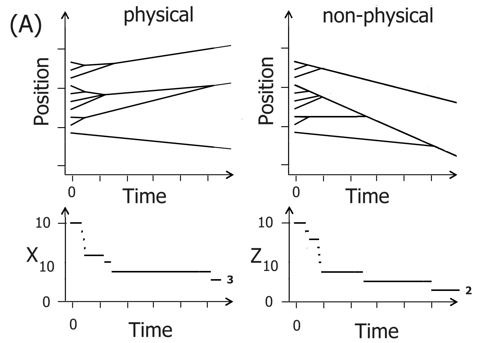
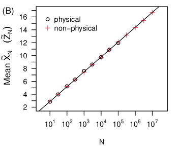
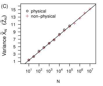
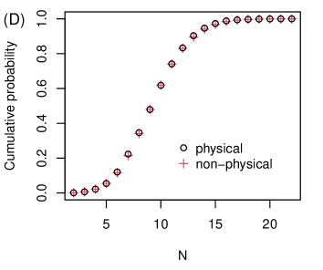
Figure 1: Example of the evolution of a system of $N=10$ particles suffering: perfectly plastic collisions, and non-physical fusion collisions. (B) Mean and (C) variance of the number of final particles as a function of the number of initial identical particles for both processes. Lines corresponds to (B) $\ln(N)+\gamma$ and (C) $\ln(N)+\gamma-\pi^{2}/6$. For each value of $N$ one (ten) thousand realizations were done for the physical (non-physical) system. (D) The empirical probability distribution of the number of final particles for $N=10000$. The estimation is based on ten thousand realizations for both systems.

II.2 A formula for $\tilde{X}_{N}$ and the mass distribution

For any given initial condition, the way to achieve the number of final particles ($\tilde{X}_{N}$) and their masses has been to evolve the particles system numerically and study the results. However, is there a way to calculate these values without evolving the system? The main purpose of this section is to show that it is possible, and to present a proposal for calculating both $\tilde{X}_{N}$ and the mass of each final particle, without time evolution.

The realization of the physical process with 10 particles shown in Fig. 1A shows, that after a transient period, the number of particles stabilises to three. When looking at the mass of these three resulting particles and comparing them to the mass of the initial particles, one of them will have three times de original value; another, six times the original value; and the last one, the one which has not collided with any particles, will have the same mass of the original particles. In other words, the final masses are $\mathbb{M}=(3,6,1)$ with a representation that considers the first coordinate of this vector to be the particle with the farthest left position, the second the next, and so on.

To introduce Theorem 2, a result regarding the velocity of a merged particle and auxiliar definitions must be presented. Let $\Theta_{i,j}:=\{k\in\mathbb{N}:i\leq k\leq j\}$ and $\overline{V}_{i,j}:=\frac{1}{j-i}\underset{k\in\Theta_{i,j}}{\sum}V_{k}$ be the average velocity of the original initial velocities of particles $i,i+1,\dots,j$ with $i\leq j$. When two particles with masses $m_{1}$ and $m_{2}$ and velocities $V_{1}$ and $V_{2}$ respectively collide, the fused particle of mass $m_{1}+m_{2}$ has a velocity equal to $V_{1}p_{1}+V_{2}(1-p_{1})$ with $p_{1}=m_{1}/(m_{1}+m_{2})$. Calculating the velocity of a system of particles of equal masses, such as the one in this case, is surprising simple: the final velocity of any fused particle, $\tilde{V}_{f}$, formed by $N_{f}$ identical particles, such as particles $k,k+1,\dots,k+N_{f}-1$, ends up being the average velocity of the fused particles,

$$\tilde{V}_{f}=\overline{V}_{k,k+N_{f}-1}.$$ (10)

Note that no hypothesis about the order of the collisions that finally formed the fused particle has been made, so eq. 10 holds no matter how all the collisions occur (see Appendix C for proof).

For the physical process, a strategy similar to the one presented for the non-physical one will be used. Consider the vector $v_{i}$, representing the initial velocities of the $N$ particles, expressed as $v_{i}=(V_{1},V_{2},\dots,V_{N})$. Let $v$ be a general vector obtained by potentially excluding the first coordinates, such as $v$ = ($V_{4},V_{5},\dots,V_{N}$). The set of all real vectors $v$ with lengths ranging from 1 to $N$ will be referred to as $\Lambda:=\underset{k\in\Theta_{N}}{\cup}\mathbb{R}^{k}$.

Definition 5

Let $\tilde{m}:\Lambda\to\Theta_{N}$ be the function

$$\tilde{m}(v)=\min\{j\in\Theta_{1,L(v)}:\overline{v}_{1,j}<\overline{v}_{j+1,i}\quad\forall i\in\Theta_{j+1,L(v)+1}\}$$

where $\overline{v}_{i,j}=\frac{1}{j-i}\overset{j}{\underset{k=i}{\sum}}w[k]$, with

$$w[k]=\left\{\begin{array}[]{lll}v[k]&&\mbox{if}\ \ k\in\Theta_{L(v)}\\ 2\max\{v[1],v[2],\dots,v[L(v)]\}&&\mbox{if}\ \ k=L(v)+1.\end{array}\right.$$

By hypothesis, the velocities are independent continuous random variables, so there will be no repeated values. Therefore, $\tilde{m}(v)$ adopts a unique value.

Definition 6

Let $G$ be a function that verifies

$$G(v)=\left\{\begin{array}[]{lll}v[(\tilde{m}(v)+1):L(v)]&&\mbox{if}\ \ L(v)>\tilde{m}(v)\\ \emptyset&&\mbox{if}\ \ L(v)=\tilde{m}(v).\end{array}\right.$$

The last condition includes $G(\emptyset)=\emptyset$

Definition 7

Let $R_{k}$ be the k-times composition of the function $G$, with $R_{0}$ the identity function. For example, $R_{3}(v)=G(G(G(v)))$.

Theorem 2

It is possible to calculate the number of final particles ($\tilde{X}_{N}$) and their individual masses ($\mathbb{M}$) without evolving the particle system (in time). Moreover, for a given initial velocity vector $v_{i}=(V_{1},V_{2},\dots,V_{N})$,

$$\tilde{X}_{N}(v_{i})=min\{k\in\Theta_{N}:R_{k}(v_{i})=\emptyset\},$$ (11)

$$\mathbb{M}(v)=(\tilde{m}(R_{0}(v_{i})),\tilde{m}(R_{1}(v_{i})),\tilde{m}(R_{2}(v_{i})),\dots,\tilde{m}(R_{\tilde{X}_{N}(v_{i})-1}(v_{i}))).$$ (12)

See Appendix D for proof. Based on the previous Theorem, a simple algorithm for computing $\tilde{X}_{N}$ and $\mathbb{M}$ is presented in Appendix E. Finally, an example is presented.

Example 2

Let $v_{i}=(5.4,2.1,8.5,1.3,9.5,3.7,10.1,7.7,4.6,6.5)$, then:

$$\begin{array}[]{lcl}\tilde{m}(v_{i})=2&&R_{1}(v_{i})=(8.5,1.3,9.5,3.7,10.1,7.7,4.6,6.5),\\ \tilde{m}(R_{1}(v_{i}))=2&&R_{2}(v_{i})=(9.5,3.7,10.1,7.7,4.6,6.5),\\ \tilde{m}(R_{2}(v_{i}))=2&&R_{3}(v_{i})=(10.1,7.7,4.6,6.5),\\ \tilde{m}(R_{3}(v_{i}))=4&&R_{4}(v_{i})=\emptyset,\end{array}$$

$\tilde{X}_{10}(v_{i})=4$, and $\mathbb{M}(v_{i})=(2,2,2,4)$.

Next, a detailed exploration of the mass distribution is presented. First, the vector $S_{N}:=\frac{\mathbb{M}}{N}$ is defined: it considers the sizes of the final particles as fractions of the original number of particles. Note that $S_{N}$ is a random vector of random length. So, in order to study this vector, $S_{N,n}:=S_{N}|(\tilde{X}_{N}=n)$ must first be defined as the conditional random vector of length equal to $n$ ($L(S_{N})=\tilde{X}_{N}$ and $L(S_{N,n})=n$).

Let $\tilde{S}_{N,n}$ be a random coordinate of the vector $S_{N,n}$, i.e. $\tilde{S}_{N,n}:=S_{N,n}[W]$, with $W$ being a random variable that takes the values $1,2,\dots,n$ with equal probability. Figure 2 shows the empirical results of $\mathbb{P}(\tilde{S}_{N,n}>s)$ as a function of $s$ for $N=10000$ and $n=[\langle\tilde{X}_{10000}\rangle]=10$ as the rounded value of the expected value of the number of final particles considering eq. 4 and 6. Data of both physical and non-physical processes is presented in a log-$x$ scale. Note that the physical and non-physical processes have the same behavior once more. In the case $n=[\langle\tilde{X}_{N}\rangle]$, it mostly behaves as

$$\mathbb{P}(\tilde{S}_{N,n}>s)\approx a_{N}\ln(s),$$

where $a_{N}$ is a constant that depends on $N$. For the case under studied in Fig. 2, $a_{N}\approx-0.1$. For values of $n$ that differ from $[\langle\tilde{X}_{N}\rangle]$, this logarithmic behavior changes principally at the highest ($1$) and lowest values ($1/N$) of $s$, see Appendix F for details.

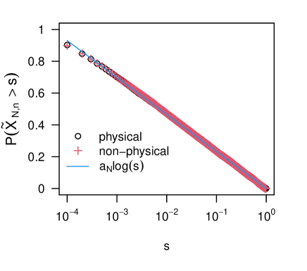
Figure 2: $\mathbb{P}(\tilde{S}_{N,n}>s)$ as a function of $s$ for $N=10000$ and $n=10$.

Understanding the behavior for different values of $n$ can be difficult; out of the most common distributions, the most consistent with the data shown in Fig. 2 is a Beta, however, confirmation that it is a discrete version of a Beta distribution has not yet been achieved. The behavior of $\mathbb{P}(\tilde{S}_{N}>s)$ is similar to the conditional probability for $n=[\langle\tilde{Z}_{N}\rangle]$, i.e. $\mathbb{P}(\tilde{S}_{N}>s)\approx\mathbb{P}(\tilde{S}_{N,[\langle\tilde{Z}_{N}\rangle]}>s)$.

II.3 Kinetic energy loss

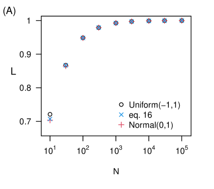
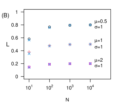
Figure 3: Proportion of the initial energy lost by total collisions as a function of the initial number of identical particles, considering random initial velocities with (A) symmetric distributions: Normal($\mu=0,\sigma=1$) and Uniform(-1,1); and (B) asymmetric distributions: Normal($\mu=\{0.5,1,2\},\sigma=1$). The theoretical values of $L$ presented in eq. 13 are represented by crosses in both graphs.

In every plastic collision, a fraction of the total energy of the colliding particles is lost. This fraction of energy lost, $(E_{initial}-E_{final})/E_{initial}$, takes values in the interval (0,1). It is equal to 1 in a frontal collision with both having equal absolute momentum values, and is close to 0 in a collision of particles with almost equal velocity. Starting from $N$ particles, the total number of collisions is $N-\tilde{Z}_{N}$, i.e. it is of the order of the number of particles. Therefore, the amount of energy lost is expected to be large, or, alternatively, a fraction of it is expected to be large. Exactly how large, be it close to 1 or 0.1, is not evident.

Figure 3A shows the average fraction of energy lost,

$$\langle L\rangle:=\langle\frac{E_{initial}-E_{final}}{E_{initial}}\rangle,$$

as a function of system size ($N$). Given that the initial energy is $E_{initial}=1/2\overset{N}{\underset{i=1}{\sum}}mV_{i}^{2}$, then the final energy will be $E_{final}=\overset{\tilde{X}_{N}}{\underset{i=1}{\sum}}1/2m_{i}\tilde{V}_{i}^{2}$, with $\overset{\tilde{X}_{N}}{\underset{i=1}{\sum}}m_{i}=Nm$, where $V_{i}$ is the initial velocity of the particle $i$, and $\tilde{V}_{i}$ is the final velocity of the (fused) particle $i$. This figure shows that very similar results are obtained for both Uniform(-1,1) and Normal(0,1) initial velocity distributions. Furthermore, similar results are obtained for other symmetric distributions around zero, such as a double exponential (data not shown). As seen in the figure, as $N$ increases, the fraction of energy loss increases as well, reaching high levels; over 99% of energy loss for relatively small systems of 1000 particles. Moreover, $L\to 1$ in the thermodynamic limit. It is worth emphasizing that, as seen in the observations, the results for small values of N (see N=10 in the graph) are dependent on the velocity distribution. While the velocity distribution had no impact on the previous sections’ results, the energy loss, conversely, is influenced by this distribution. Understanding the energy loss calculation requires knowledge of the velocity difference between colliding particles, denoted as $\Delta V:=V_{1}-V_{2}$. It’s crucial to acknowledge that the distribution of the subtraction of two independent continuous random variables is not universal; each velocity distribution $F$ yields a distinct distribution for $\Delta V$. Therefore, the significance of the velocity distribution is highlighted in this section.

In order to get a theoretical approximation regarding the energy loss, an informal argument about the approximate behaviour of the particle system in a one dimensional space will be explored. Initially, two “types of particles” will be considered: those composed of a large number of merged particles, and those composed of a small number of merged particles, henceforth called $C$ (central) particles and $B$ (border) particles respectively. The large particles are those that grow linearly with $N$, and the small particles are those that grow sublinearly. The particles that don’t start at the ends (i.e. not in the first nor the last positions) will eventually collide and form these large particles ($C$ particles) at the end of the process. On the other hand, particles that start at the ends (or borders) can “get away” and suffer very few collisions in this “escape”, becoming $B$ particles. The expected velocity of $B$ particles will be similar to the velocity of the original particles since they will suffer few to no collisions. In contrast, the velocity of $C$ particles will be very different from that of $B$ particles. As explained in the previous section, the velocity of fused particles (eq. 10) is an average of independent velocities, meaning that for large fused particles, the velocity will be very close to the initial expected velocity, $\langle V\rangle$. In fact, the variance of the velocity of a fused particle is equal to the variance of the initial velocity divided by the number of particles that form the fused particle ($N_{f}$), i.e.

$$\langle\tilde{V}_{f}^{2}\rangle=\langle V\rangle^{2}+\frac{\langle V^{2}\rangle-\langle V\rangle^{2}}{N_{f}}.$$

The above expression will be used to calculate the velocity of merged $C$ particles. In the case of $B$ particles, the velocity will be approximated by using the initial velocity of the original particle, as if no collision had occurred. Furthermore, a fraction $b$ of the final $\tilde{X}_{N}$ particles will be considered as particles of type $B$, while the remainder will be treated as merged $C$ particles, with each of them formed by $(N-b\tilde{X}_{N})/((1-b)\tilde{X}_{N})$ particles. With all the above considerations, the mean final energy can be written as:

$$\begin{split}&\langle E_{final}\rangle\approx 1/2b\langle\tilde{X}_{N}\rangle m\langle V^{2}\rangle\\ &+1/2(N-b\langle\tilde{X}_{N}\rangle)m\left(\langle V\rangle^{2}+\frac{(\langle V^{2}\rangle-\langle V\rangle^{2})(1-b)\langle\tilde{X}_{N}\rangle}{N-b\langle\tilde{X}_{N}\rangle}\right),\end{split}$$

that does not depend on $b$. Therefore, the expected fraction of kinetic energy lost,

$$\langle L\rangle\approx 1-\frac{\langle\tilde{X}_{N}\rangle}{N}-(1-\frac{\langle\tilde{X}_{N}\rangle}{N})\frac{\langle V\rangle^{2}}{\langle V^{2}\rangle}.$$ (13)

Note that, for large $N$, this loss of energy $\langle L\rangle$ goes to a value that depends only on the quotient of the first two moments of the velocity distribution. In particular, for velocity distributions with $\langle V\rangle=0$ or $\langle V^{2}\rangle=\infty$, all kinetic energy is lost in the thermodynamic limit.

Panel B in Figure 3 is similar to panel A, but in this case, results show for a Normal initial velocity distribution, which is centered at various non-zero values (Normal($\mu=\{0.5,1,2\},\sigma=1$)). Note that the asymptotic value of $\langle L\rangle$ is now different from 1. For example, the Normal distribution centered at 1 with variance equal to 1 (and $\langle V^{2}\rangle=2$) goes to approximately 1/2.

In panels A and B of Fig. 3, the theoretical approximation given by eq. 13 is represented by crosses. Note that the theoretical approximation for $\langle L\rangle$ is highly accurate in the asymptotic case, and it is also accurate for small values of $N$. Finally, to test the validity of the theoretical approximation given by eq. 13, further velocity distribution were studied by simulating the particle systems for a size of $N=10000$. Table 2 shows the results obtained. Note that the empirical results seem to coincide with the theoretical values in each type of distributions studied, validating our approximation.

Distribution	Empirical	Theoretical
Normal(0,1)	0.99901 $\pm$ 0.00003	0.99902
Beta(1,1)	0.24973 $\pm$ 0.00017	0.24976
Beta(2,2)	0.16661 $\pm$ 0.00012	0.16650
Beta($\frac{1}{2}$,$\frac{1}{2}$)	0.33310 $\pm$ 0.00021	0.33301
Gamma(1,1)	0.49936 $\pm$ 0.00031	0.49951
Gamma(1,5)	0.49945 $\pm$ 0.00031	0.49951
Gamma(5,1)	0.16653 $\pm$ 0.00013	0.16650

Table 2: Empirical and theoretical values of the expected fraction of energy loss, $\langle L\rangle$, for different initial velocity distributions, and considering a system of $N=10000$ initial particles.

II.4 Explosion-like inital condition

In this section, the same system of particles will be studied, however, a different initial condition will be applied. This initial condition will consider particles placed at negative initial positions starting with negative random velocities, and particles positioned at positive initial positions starting with positive random velocities. This initial condition mimics an explosion at the origin.

Since particles with positive initial positions will never interact with particles on the left, the result of this particular “explosive” initial condition is the superposition of the results of two independent systems: the right and the left one. Therefore, the expected number of final particles in this condition, $\langle\tilde{X}^{expl}_{N}\rangle$, is only $2\langle\tilde{X}_{N/2}\rangle$ when half of the particles are on each side. For a random distribution of $N$ particles on two sides,

$$\langle\tilde{X}^{expl}_{N}\rangle=\overset{N}{\underset{k=0}{\sum}}\mathbb{P}(N_{\leftarrow}=k)(\langle\tilde{X}_{k}\rangle+\langle\tilde{X}_{N-k}\rangle),$$

where $\mathbb{P}(N_{\leftarrow}=k)$ is the probability that $k$ of the $N$ initial particles start on the left, and $\langle\tilde{X}_{1}\rangle=1$, and $\langle\tilde{X}_{0}\rangle=0$. Since both sides are independent, the variance is the sum of the variances on each side. Moreover, the distribution of $\tilde{X}^{expl}_{N}$ for a random sorting of $N$ particles on each side of the axis will verify,

$$\mathbb{P}(\tilde{X}^{exp}_{N}=j)=\overset{N}{\underset{k=0}{\sum}}\overset{j}{\underset{l=0}{\sum}}\mathbb{P}(N_{\leftarrow}=k)\mathbb{P}(\tilde{X}_{k}=l)\mathbb{P}(\tilde{X}_{N-k}=j-l).$$

III Conclusions

A 1D particle system of $N$ identical point particles undergoing plastic collisions has been studied. Explicit expressions for the mean and variance of the final number of particles, as well as an accurate approximation for the energy loss, were found. It was also shown that, in order to compute the final mass distribution, evolving the particle system is not necessary. Calculating it by simply considering the initial velocity and position of each particle in 1D has been proven to be an alternative approach of lower computational cost.

Some of these results have been obtained thanks to the introduction of a new system of particles, here called non-physical. Although most realizations under the same initial conditions yielded different results (see Fig. 1A), surprisingly, the results for the non-physical systems are statistically equivalent to the physical ones. This is similar to the universality classes of systems in the critical regime of phase transitions, where different models behave in the same way [12, 13]. That rises the question: are there “universality” classes for non-equilibrium systems like the one presented in this paper? Results show that both, the physical and the non-physical model, behave in the same way. This is compatible with a vision that proposes that both models belong to the same model category. Admittedly. looking into the existence of classes of mathematical models for non-equilibrium systems lacking a phase transition is not only fascinating, but it could also aid in better understanding non-equilibrium systems.

Finally, it is likely there are some challenges in trying to extend the system presented here to larger dimensions. In this case, it is necessary to adapt the point particles to finite particles in order for collisions to happen, and of course, it is also necessary to modify the initial conditions. It is expected for the number of final particles ($\tilde{X}_{N}$) to increase along with the dimension of space, as well as for the distribution of the final particle masses to change; however, the decreasing monotonic behavior of the probability density is expected to stay the same. In order to properly calculate these statistical properties it is fundamental to consider a key variable: the percentage of the total particles that can be considered at the surface (or that belongs to the “propagating wavefront”). Typically, superficial particles are likely to “escape”, experiencing a small number of plastic collisions in the process. On the other hand, those that start closer to the center will suffer significantly more collisions, becoming considerably massive particles. Therefore, as a general rule, for non-explosive random initial conditions, one would say that the final particles that are farther away from the starting point will most likely be lower-mass particles. Conversely, under explosive initial condition, the lower mass particles are likely to be both those farther away and those closer to the starting point.

From a modeling perspective, the findings outlined in this study could potentially pave the way for the development of more intricate models that closely mirror real-world scenarios. The concepts and outcomes presented in this paper might prove valuable in understanding and addressing other non-equilibrium processes. To use an analogy, plastic collisions are to final particles what gravity is to galaxies: just like stars and interstellar matter are bound together by gravity, original particles are bound by plastic collisions. I believe that the results and concepts presented in this paper may have additional value in the eyes of an astrophysicist.

Appendix A: Variance of $\tilde{Z}_{N}$ and $\tilde{X}_{N}$ for small N

$$\mbox{Var}(\tilde{Z}_{N})=\frac{1}{N!}\overset{N!}{\underset{k=1}{\sum}}\tilde{Z}^{2}_{N}(\omega_{k})-(\frac{1}{N!}\overset{N!}{\underset{k=1}{\sum}}\tilde{Z}_{N}(\omega_{k}))^{2}$$

N	Var($\tilde{Z}_{N}$)	Var($\tilde{X}_{N}$)
2	$\frac{1}{4}$	$\frac{1}{4}$
3	$\frac{17}{36}$	$\frac{17}{36}$
4	$\frac{95}{144}\approx 0.6597$	[0.6532, 0.6745]
5	$\frac{274}{120}\approx 0.8197$	[0.8044, 0.8306]
6	$\frac{3451}{3600}\approx 0.9586$	[0.9437, 0.9744]
7	$\frac{190699}{176400}\approx 1.0811$	[1.0555, 1.0898]
8	$\frac{839971}{705600}\approx 1.1904$	[1.1580, 1.1956]
9	$\frac{8186939}{6350400}\approx 1.2892$	[1.2807, 1.3223]
10	$\frac{350339}{254016}\approx 1.3792$	[1.3589, 1.4031]

Table 3: *

Table S1. Exact Var($\tilde{Z}_{N}$) and approximate Var($\tilde{X}_{N}$) for different values of $N$. The approximate data correspond to the 95% confidence interval [$(n-1)s^{2}/\chi^{2}_{0.025,n-1},(n-1)s^{2}/\chi^{2}_{0.975,n-1}$] obtained from n=30000 simulations. For $N=2$ and 3 only exact results are presented.

Appendix B: Proof of Theorem 1

Let define the function $G_{k}:\Omega_{N}\to\Omega_{N+1}$ with $k\in\Theta_{N+1}$ by following way:

$$G_{k}(\mathbf{s}_{N})=(s_{1},s_{2},\dots,s_{k-1},N+1,s_{k},s_{k+1},\dots,s_{N}).$$

For example, if $\omega=(4,2,1,3,6,5)$, then $G_{4}(\omega)=(4,2,1,7,3,6,5)$ and $G_{7}(\omega)=(4,2,1,3,6,5,7)$.

Note that

$$\Omega_{N+1}=\underset{i\in\Theta_{N+1}}{\cup}\underset{\omega\in\Omega_{N}}{\cup}G_{i}(\omega).$$

Now, it is easy to see that for every $\omega\in\Omega_{N}$

$$\tilde{Z}_{N+1}(G_{k}(\omega))=\left\{\begin{array}[]{lll}\tilde{Z}_{N}(\omega)&&\mbox{if}\ \ k\neq N+1\\ \tilde{Z}_{N}(\omega)+1&&\mbox{if}\ \ k=N+1.\end{array}\right.$$ (14)

$$\begin{split}\langle\tilde{Z}_{N+1}\rangle&=\frac{1}{(N+1)!}\underset{\omega\in\Omega_{N+1}}{\sum}\tilde{Z}_{N+1}(\omega)\\ &=\frac{1}{(N+1)!}\overset{N+1}{\underset{k=1}{\sum}}\underset{\omega\in\Omega_{N}}{\sum}\tilde{Z}_{N+1}(G_{k}(\omega))\\ &=\frac{1}{(N+1)!}(\overset{N}{N\underset{\omega\in\Omega_{N}}{\sum}}\tilde{Z}_{N}(\omega)+\underset{\omega\in\Omega_{N}}{\sum}(\tilde{Z}_{N}(\omega)+1))\\ &=\frac{1}{(N+1)!}((N+1)!\langle\tilde{Z}_{N}\rangle+N!)\\ &=\langle\tilde{Z}_{N}\rangle+\frac{1}{N+1}.\end{split}$$ (15)

Finally, taking into account that $\tilde{Z}_{1}=1$, we obtain $\langle\tilde{Z}_{N}\rangle=\overset{N}{\underset{k=1}{\sum}}\frac{1}{k}$, which concludes the proof.

A similar calculation is performed to prove eq. 7 obtained for the variance.

$$\begin{split}\langle\tilde{Z}_{N+1}^{2}\rangle&=\frac{1}{(N+1)!}\underset{\omega\in\Omega_{N+1}}{\sum}(\tilde{Z}_{N+1}(\omega))^{2}\\ &=\frac{1}{(N+1)!}\overset{N+1}{\underset{k=1}{\sum}}\underset{\omega\in\Omega_{N}}{\sum}(\tilde{Z}_{N+1}(G_{k}(\omega)))^{2}\\ &=\frac{1}{(N+1)!}(N\underset{\omega\in\Omega_{N}}{\sum}(\tilde{Z}_{N}(\omega))^{2}+\underset{\omega\in\Omega_{N}}{\sum}(\tilde{Z}_{N}(\omega)+1)^{2})\\ &=\frac{1}{(N+1)!}((N+1)!\langle(\tilde{Z}_{N})^{2}\rangle+N!+2N!\langle\tilde{Z}_{N}\rangle\\ &=\langle\tilde{Z}_{N}^{2}\rangle+\frac{1}{N+1}(1+2\langle\tilde{Z}_{N}\rangle).\end{split}$$ (16)

The variance is calculated by

$$\sigma^{2}_{N}:=\langle\tilde{Z}_{N}^{2}\rangle-\langle\tilde{Z}_{N}\rangle^{2}.$$

In view of equations 15 and 16, we have

$$\begin{split}\sigma^{2}_{N+1}&=\langle\tilde{Z}_{N}^{2}\rangle+\frac{1}{N+1}(1+2\langle\tilde{Z}_{N}\rangle)-(\langle\tilde{Z}_{N}\rangle+\frac{1}{N+1})^{2}\\ &=\sigma^{2}_{N}+\frac{1}{N+1}(1)-(\frac{1}{N+1})^{2}\\ &=\sigma^{2}_{N}+\frac{1}{N+1}(1-\frac{1}{N+1})\\ &=\sigma^{2}_{N}+\frac{N}{(N+1)^{2}}.\\ \end{split}$$ (17)

Finally, since $\sigma^{2}_{1}=0$,

$$\sigma^{2}_{N}=\overset{N}{\underset{i=1}{\sum}}\frac{i-1}{i^{2}}=\overset{N}{\underset{i=1}{\sum}}\frac{1}{i}-\overset{N}{\underset{i=1}{\sum}}\frac{1}{i^{2}}.$$

Appendix C: The velocity of the fused particle

Definition 8

A (snowball) S-fused particle is a fused particle that is formed by collisions between a fused particle and a (non-fused) particle of mass m, except for the first collision which is between two particles of mass m.

To prove Eq. 10, let’s start by noting that every fused particle is either an S-fused particle or the result of the collision of two or more S-fused particles. Let’s then calculate the velocity of an S-fused particle. For instance, if the S-fused particle is formed by three particles (each with a mass of $m$), then it has a velocity,

$$\tilde{\tilde{v}}_{f}:=(v_{1}p_{1}+v_{2}(1-p_{1}))p_{2}+v_{3}(1-p_{2})=\frac{1}{3}\overset{3}{\underset{j=1}{\sum}}v_{j},$$

with $p_{k}=\frac{k}{k+1}$, and $v_{1},v_{2},v_{3}$ the velocities of the particles, considering the natural order (lef-right or right-left), where particle 1 is the one that participates in the first collision. Note that $\tilde{\tilde{v}}_{f}$ is the average velocity of the 3 particles. For the general case where the mass of the S-fused particle is equal to $km$, it is easy to see that the velocity of this fused particle is

$$\begin{split}\tilde{\tilde{v}}_{f}&=v_{1}\overset{k-1}{\underset{i_{1}=1}{\prod}}\frac{i_{1}}{i_{1}+1}+v_{2}\frac{1}{2}\overset{k-1}{\underset{i_{2}=2}{\prod}}\frac{i_{2}}{i_{2}+1}+v_{3}\frac{1}{3}\overset{k-1}{\underset{i_{3}=3}{\prod}}\frac{i_{3}}{i_{3}+1}\\ &+\dots+v_{k-1}\frac{1}{k-1}\overset{k-1}{\underset{i_{k-1}=k-1}{\prod}}\frac{i_{k-1}}{i_{k-1}+1}+v_{k}\frac{1}{k}\\ &=\frac{1}{k}\overset{k}{\underset{j=1}{\sum}}v_{j},\end{split}$$

equal to the average velocity. Now, if an S-fused particle of size $k_{1}$ fuses with another S-fused particle of size $k_{2}$, then the new fused particle of size $k_{1}+k_{2}$ has a velocity equal to the weighted average of the velocities of the S-fused particles,

$$\begin{split}&(\frac{1}{k_{1}}\overset{k_{1}+h-1}{\underset{i=h}{\sum}}v_{i})\frac{k_{1}}{k_{1}+k_{2}}+(\frac{1}{k_{2}}\overset{k_{2}+k_{1}+h-1}{\underset{i=k_{1}+h}{\sum}}v_{i})\frac{k_{2}}{k_{1}+k_{2}}\\ &=\frac{1}{k_{1}+k_{2}}\overset{k_{1}+k_{2}}{\underset{i=1}{\sum}}v_{i},\end{split}$$

which is exactly the average velocity of all particles involved, concluding the proof.

Appendix D: Proof of Theorem 2

The process begins with a configuration of velocities $v_{1}:=v_{i}=(V_{1},V_{2},\dots,V_{N})$ and a set of positions $Y_{1}<Y_{2}<\dots<Y_{N}$. The specific positions determine the sequence of collisions, dictating which ones occur initially and which ones follow. Importantly, this sequence doesn’t impact the total number of final particles or the mass of each individual particle. For a detailed proof, refer to the end of this appendix. Consequently, in the following, we will assume a particular order in which the collisions take place

For particles 1 and 2 to merge, one of two alternatives must occur: (A) $V_{1}>V_{2}$, or (B) $V_{1}>\frac{1}{s-1}\overset{s}{\underset{i=2}{\sum}}V_{i}$ for some $s>2$ (i.e. particle 1 collide with a fused particle that contains particle 2). Alternatively, we can express that particle 1 merges with other particles if $s_{1}(v_{i})\neq\emptyset$, where

$$s_{1}(v_{1})=\min\{s\in\Theta_{2,N}:V_{1}>\overline{V}_{2,s}\},$$

with $\overline{V}_{j,k}=\frac{1}{k-j}\overset{k}{\underset{i=j}{\sum}}V_{i}$. If $s_{1}(v_{1})\neq\emptyset$, particle 1 will collide with a merged particle comprising particles $2,3,\dots,s_{1}(v_{1})$. In essence, a merged particle will form, incorporating particles $1,2,\dots,s_{1}(v_{1})$, and it will have a velocity $\overline{V}_{1,s_{1}(v_{1})}$.

Now, with this new merged particle, we work as we did before, i.e. as if it were the original particle 1, which can be merged when $s_{2}(v_{1})\neq\emptyset$, where

$$s_{2}(v_{1})=\min\{s\in\Theta_{s_{1}+1,N}:\overline{V}_{1,s_{1}}>\overline{V}_{s_{1}+1,s}\}.$$

If $s_{2}(v_{1})\neq\emptyset$, then the merged particle containing particles $1,2,\dots,s_{1}(v_{1})$ will inevitably collide with another merged particle containing particles $s_{1}(v_{1})+1,3,\dots,s_{2}(v_{1})$. Consequently, a new merged particle will form, incorporating particles $1,2,\dots,s_{2}(v_{1})$, and it will possess a velocity of $\overline{V}_{1,s_{2}(v_{1})}$. This process repeats until, for the first time,

$$\tilde{k}(v_{1})=\min\{k\in\Theta_{N}:s_{k}(v_{1})=\emptyset\ or\ s_{k}(v_{1})=N\}.$$

with

$$s_{k}(v_{1})=\min\{s\in\Theta_{s_{k-1}(v_{1})+1,N}:\overline{V}_{s_{0}(v_{1}),s_{k-1}(v_{1})}>\overline{V}_{s_{k-1}(v_{1})+1,s}\},$$

and $s_{0}(v_{1})=1$.

Finally, the resulting final particle 1, the leftmost particle, will be a fusion of particles $1,2,\dots,s_{\tilde{k}(v_{1})}(v_{1})$. That is, the mass will be $s_{\tilde{k}(v_{1})}(v_{1})$, and if its mass is smaller than $N$, the following condition will be satisfied :

$$\overline{V}_{1,s_{\tilde{k}(v_{1})}(v_{1})}<\overline{V}_{s_{\tilde{k}(v_{1})}(v_{1})+1,s}\quad\forall s\in\Theta_{s_{\tilde{k}(v_{1})}+1,N}.$$ (18)

The general case of $s_{\tilde{k}(v_{1})}(v_{1})$, which includes the value $N$, can be written as:

$$\begin{split}s_{\tilde{k}(v_{1})}&(v_{1})=\tilde{m}(v_{1})\\ &=\min\{j\in\Theta_{1,N}:\overline{V}_{1,j}<\overline{V}_{j+1,i}\quad\forall i\in\Theta_{j+1,N+1}\}.\end{split}$$ (19)

Where, to improve the notation, an additional “phantom” particle is added; particle $N+1$, positioned to the right of particle $N$, with a velocity equal to $2V_{\text{max}}:=2\max\{V_{1},V_{2},\dots,V_{N}\}$. The upper row in Fig. S1 presents an illustration of a system involving $N=9$ particles, solved through the temporal evolution of the process. In contrast, the analogous scenario without temporal evolution, as outlined by equation 19, is portrayed in the upper row of Fig. S2.

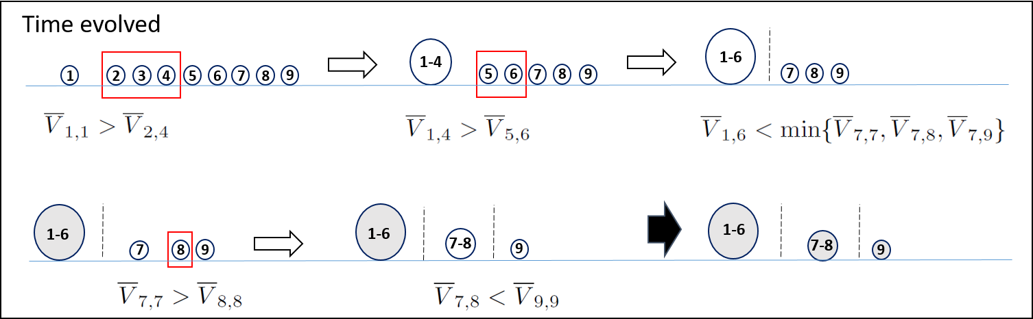
Figure 4: *

Fig. S1. Solution based on system evolution.

Now that we understand the composition of the final particle 1, comprising particles $1,2,\dots,\tilde{m}(v_{1})$, we can apply a similar analysis to the remaining particles on the right-hand side. Assuming $\tilde{m}(v_{1})<N$, we initiate the analysis starting with particle $\tilde{m}(v_{1})+1$ to investigate potential mergers with the remaining particles. Let $v_{2}=v_{1}[\tilde{m}(v_{1})+1:N]$=($V_{\tilde{m}(v_{1})+1},V_{\tilde{m}(v_{1})+2},\dots,V_{N}$) and define

$$s_{1}(v_{2})=\min\{s\in\Theta_{\tilde{m}(v_{1})+2,N}:V_{\tilde{m}(v_{1})+1}>\overline{V}_{\tilde{m}(v_{1})+2,s}\}.$$

If $s_{1}(v_{2})\neq\emptyset$, particle $\tilde{m}(v_{1})+1$ will collide with a merged particle comprising particles $\tilde{m}(v_{1})+2,\tilde{m}(v_{1})+3,\dots,s_{1}(v_{2})$. A merged particle will form, incorporating particles $\tilde{m}(v_{1})+1,\tilde{m}(v_{1})+2,\dots,s_{1}(v_{2})$, and it will have a velocity $\overline{V}_{\tilde{m}(v_{1})+1,s_{1}(v_{2})}$. This fused particle can fuse with other particles if $s_{2}(v_{2})\neq\emptyset$, with

$$s_{2}(v_{2})=\min\{s\in\Theta_{s_{1}(v_{2})+2,N}:\overline{V}_{s_{1}(v_{2})+1,s}>\overline{V}_{s_{1}(v_{2})+2,s}\}.$$

If $s_{2}(v_{2})\neq\emptyset$, the fused particle will collide. The new fused particle will be formed by particles $s_{1}(v_{1})+1,s_{1}(v_{1})+2,\dots,s_{2}(v_{2})$, and this process continues until the first time that

$$\tilde{k}(v_{2})=\min\{k\in\Theta_{N}:s_{k}(v_{2})=\emptyset\ or\ s_{k}(v_{2})=N\}.$$

with

$$s_{k}(v_{2})=\min\{s\in\Theta_{s_{k-1}(v_{2})+1,N}:\overline{V}_{s_{0}(v_{2}),s_{k-1}(v_{2})}>\overline{V}_{s_{k-1}(v_{2})+1,s}\},$$

and $s_{0}(v_{2})=s_{\tilde{k}(v_{1})}(v_{1})+1$. It is crucial to reemphasize that, within the context of this proof,

$$s_{\tilde{k}(v_{2})}(v_{2})=\tilde{m}(v_{2}).$$

This continues until we have $\tilde{j}$ final particles, with

$$\tilde{j}=\min\{j\in\Theta_{N}:\overset{j}{\underset{h=1}{\sum}}\tilde{k}(v_{h})=N\}.$$

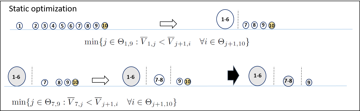
Figure 5: *

Fig. S2. Solution without relying on system evolution.

Finally, evolving the system, we obtain the following final masses:

$$\begin{split}\mathbb{M}&=(s_{\tilde{k}(v_{1})}(v_{1}),s_{\tilde{k}(v_{2})}(v_{2}),\dots,s_{\tilde{k}(v_{\tilde{j}})}(v_{\tilde{j}})),\\ &=(\tilde{m}(v_{1}),\tilde{m}(v_{2}),\dots,\tilde{m}(v_{\tilde{j}})),\\ &=(\tilde{m}(R_{0}(v_{i})),\tilde{m}(R_{1}(v_{i})),\dots,\tilde{m}(R_{\tilde{X}_{N}(v_{i})-1}(v_{i}))).\end{split}$$

To conclude the proof, note that the last equality is valid, since $v_{j}=R_{j-1}(v_{i})$ and

$$\begin{split}\tilde{X}_{N}(v_{i})&=min\{k\in\Theta_{N}:R_{k}(v_{i})=\emptyset\},\\ &=min\{k\in\Theta_{N}:\overset{k-1}{\underset{j=0}{\sum}}\tilde{m}(R_{j}(v_{i}))=N\}.\end{split}$$

Proof that Initial positions have no effect on $\mathbb{M}$

Suppose $N$ particles start at positions $Y_{1}<Y_{2}<\dots<Y_{N}$ and with velocities $V_{1},V_{2},\dots,V_{N}$ respectively. If we evolve the system, we end up with $\tilde{X}_{N}$ particles with masses $\mathbb{M}=(m_{1},m_{2},\dots,m_{\tilde{X}_{N}})$ and final velocities ($v^{f}_{1},v^{f}_{2},\dots,v^{f}_{\tilde{X}_{N}}$) with $v^{f}_{i}=\overline{V}_{M_{i-1}+1,M_{i}}$ with $M_{k}=\overset{k}{\underset{i=1}{\sum}}m_{i}$ for $k\in\Theta_{\tilde{X}_{N}}$ and $M_{0}=0$.

Final particles verify:

$$\overline{V}_{1,m_{1}}<\overline{V}_{M_{1}+1,M_{2}}<\overline{V}_{M_{2}+1,M_{3}}<\dots<\overline{V}_{\tilde{X}_{N}-1,M_{\tilde{X}_{N}}}.$$

In addition, every fused final particle verifies:

$$\overline{V}_{M_{k-1}+1,M_{k}-1}>\overline{V}_{M_{k},M_{k}}.$$ (20)

Otherwise, the last particle composing the final particle would not merge. The same argument holds for the last $j$ particles of the final particle, i.e.

$$\overline{V}_{M_{k-1}+1,M_{k}-j}>\overline{V}_{M_{k}-j+1,M_{k}}.$$ (21)

Now we study the system, but in this case, starting from different positions $Y^{new}_{1}<Y^{new}_{2}<\dots<Y^{new}_{N}$, while maintaining the previous velocities. By evolving the system, we end up with $\tilde{X}^{new}_{N}$ particles with masses $\mathbb{M}^{new}=(m^{new}_{1},m^{new}_{2},\dots,m^{new}_{\tilde{X}^{new}_{N}})$. The equation refposi2 is again fulfilled, but $M_{k}$ is replaced by $M^{new}_{k}:=\overset{k}{\underset{i=1}{\sum}}m^{new}_{k}$,

$$\overline{V}_{M^{new}_{k-1}+1,M^{new}_{k}-j}>\overline{V}_{M^{new}_{k}-j+1,M^{new}_{k}}.$$ (22)

Suppose the final configurations are different, $\mathbb{M}\neq\mathbb{M}^{new}$. Then there is a first final particle in which they are certain to differ.Without loss of generality, let us assume that this difference occurs in the first final particle, i.e. $m_{1}\neq m_{1}^{new}$.

Suppose first that $m^{new}_{1}$ is less than $m_{1}$, specifically $m^{new}_{1}=m_{1}-j$ with $j\in\Theta_{m_{1}-1}$. First note, the first final particle will always have a lower velocity than the second final particle,

$$\overline{V}_{1,m^{new}_{1}}<\overline{V}_{m^{new}_{1}+1,m^{new}_{1}+m^{new}_{2}}.$$ (23)

According to eq 22, we have that $\overline{V}_{m^{new}_{1}+1,m^{new}_{1}+m^{new}_{2}}<\overline{V}_{m^{new}_{1}+1,m^{new}_{1}+j}$. So by putting this information together, it is verified:

$$\overline{V}_{1,m^{new}_{1}}<\overline{V}_{m^{new}_{1}+1,m^{new}_{1}+j}.$$ (24)

However, if we look at the original system with the initial positions $Y_{1},Y_{2},\dots,Y_{N}$, we see that due to the equation 21, it is fulfilled:

$$\overline{V}_{1,m^{new}_{1}}=\overline{V}_{1,m_{1}-j}>\overline{V}_{m_{1}-j+1,m_{1}}=\overline{V}_{m^{new}_{1}+1,m^{new}_{1}+j}.$$ (25)

This last equation contradicts equation 24, so $m^{new}_{1}$ cannot be less than $m_{1}$.

In the same way, we can prove that $m^{new}_{1}$ cannot be greater than $m_{1}$. So $\mathbb{M}=\mathbb{M}^{new}$.

Appendix E: Algorithm for $Z_{N}$ and $\mathbb{M}$.

v[1:$N$] $\leftarrow$ randomF($N$); # N velocities

v[$N$+1] $\leftarrow 2$ $\cdot$ max(v); # auxilar velocity

vi $\leftarrow$ v ;

w $\leftarrow$ 0 ; s $\leftarrow$1

$\mathbb{M}$ $\leftarrow$ vector();

while w $<N$ do

      

      $\mathbb{M}$[s] $\leftarrow$ $\tilde{m}$(vi) ;

      w $\leftarrow$ masses[s]+w ;

      vi $\leftarrow$ v[(w+1):length(v)] ;

      s $\leftarrow$ s+1 ;

end while

$Z_{N}$ $\leftarrow$ length($\mathbb{M}$) ; # number of final particles

Algorithm 1 An algorithm for $Z_{N}$ and $\mathbb{M}$.

$\tilde{m}$=function(v){

$N\leftarrow$ length(v)-1

$\Theta$ $\leftarrow 1:N$; $\Lambda$ $\leftarrow 2:(N+1)$;

k $\leftarrow$1; i $\leftarrow$ 1;

while $\Lambda[i]$ $<$ N+1 do

      

      i $\leftarrow$ 1;

      $\Lambda$ $\leftarrow$ ($\Theta$[k]+1):$(N+1)$ ;

      vl $\leftarrow$ mean(v[1:$\Theta$[k]]);

      vr $\leftarrow$ mean(v[$\Lambda$[1]:$\Lambda$[i]]);

      k $\leftarrow$ k+1;

      while vl$<$vr & $\Lambda$[i] $<$N+1 do

            

            i $\leftarrow$ i+1 ;

            vr $\leftarrow$ mean(v[$\Lambda$[1]:$\Lambda$[i]]);

       end while

      

end while

mass $\leftarrow$ k-1;

return(mass) }

Algorithm 2 $\tilde{m}$ function.

Appendix F: Conditional Mass distribution.

Fig. S3 shows $\mathbb{P}(\tilde{S}_{N,n}>s)$ as a function of $s$ for $N=10000$ and three values of $n$.

Figure 6: *

Fig. S3. $\mathbb{P}(\tilde{S}_{N,n}>s)$ as a function of $s$ for $N=10000$ and $n=\{6,10,14\}$.

References

- [1] Fang, X., Kruse, K., Lu, T., Wang, J. (2019). Nonequilibrium physics in biology. Reviews of Modern Physics, 91(4), 045004.
- [2] Van Esch, J. H., Klajn, R., Otto, S. (2017). Chemical systems out of equilibrium. Chemical Society Reviews, 46(18), 5474-5475.
- [3] Pope S.B. (2023) Turbulent flows. Cornell University, New York.
- [4] Landi, G. T., Poletti, D., Schaller, G. (2022). Nonequilibrium boundary-driven quantum systems: Models, methods, and properties. Reviews of Modern Physics, 94(4), 045006.
- [5] Khairnar, V. D., Pradhan, S. N. (2011). Mobility models for vehicular ad-hoc network simulation. IEEE Symposium on Computers & Informatics, 460-465.
- [6] Kozlov, V. G., Skrypnikov, A. V., Samcov, V. V., Levushkin, D. M., Nikitin, A. A., Zaikin, A. N. (2019). Mathematical models to determine the influence of road parameters and conditions on vehicular speed. Journal of Physics: Conference Series, Vol. 1333, No. 3, p. 032041.
- [7] Strogatz, S. H. (2018). Nonlinear dynamics and chaos with student solutions manual: With applications to physics, biology, chemistry, and engineering. CRC press.
- [8] Hasegawa, A. (2012). Plasma instabilities and nonlinear effects (Vol. 8). Springer Science & Business Media.
- [9] McGinley, M., Cooper, N. R. (2018). Topology of one-dimensional quantum systems out of equilibrium. Physical Review Letters, 121(9), 090401.
- [10] Pietroni, M. (2009). Non-equilibrium in cosmology. The European Physical Journal Special Topics, 168(1), 149-177.
- [11] Philcox, O. H., Torquato, S. (2023). Disordered Heterogeneous Universe: Galaxy Distribution and Clustering across Length Scales.Physical Review X, 13(1), 011038.
- [12] Christensen, K., Moloney, N. R. (2005). Complexity and criticality (Vol. 1). World Scientific Publishing Company.
- [13] Ódor, G. (2004). Universality classes in nonequilibrium lattice systems. Reviews of modern physics, 76(3), 663.