Optimal Rates of Kernel Ridge Regression under Source Condition in Large Dimensions
Abstract
Motivated by the studies of neural networks (e.g.,the neural tangent kernel theory), we perform a study on the large-dimensional behavior of kernel ridge regression (KRR) where the sample size for some . Given an RKHS associated with an inner product kernel defined on the sphere , we suppose that the true function , the interpolation space of with source condition . We first determined the exact order (both upper and lower bound) of the generalization error of kernel ridge regression for the optimally chosen regularization parameter . We then further showed that when , KRR is minimax optimal; and when , KRR is not minimax optimal (a.k.a. the saturation effect). Our results illustrate that the curves of rate varying along exhibit the periodic plateau behavior and the multiple descent behavior and show how the curves evolve with . Interestingly, our work provides a unified viewpoint of several recent works on kernel regression in the large-dimensional setting, which correspond to and respectively.
Keywords: kernel methods, high-dimensional statistics, reproducing kernel Hilbert space, minimax optimality, saturation effect
1 Introduction
The recent studies of neural network theory have brought the renaissance of kernel methods, since the neural tangent kernel (Jacot et al., 2018) provides a natural surrogate to understand the wide neural network (Arora et al., 2019; Lee et al., 2019; Lai et al., 2023). When the dimension of data is fixed, there has been extensive literature studying the generalization behavior of kernel ridge regression (KRR), one of the most popular kernel methods, e.g., Caponnetto and de Vito (2007); Fischer and Steinwart (2020); Cui et al. (2021), etc.. Researchers usually use two crucial factors to characterize KRR’s generalization behavior: capacity condition and source condition. Supposing eigenvalues associated with the RKHS are , the capacity condition (also known as effective dimension) assumes for some , where will represent the regularization parameter in KRR. The capacity condition characterizes the size of and is frequently stated as an equivalent eigenvalue decay condition: . The source condition assumes that the true function falls into , an interpolation space of for some . It characterizes the relative smoothness of with respect to : the larger is, the “smoother” is and the easier it can be estimated. Under this framework, many interesting topics about KRR’s generalization behavior were studied. For instance, the minimax optimality of KRR (Fischer and Steinwart, 2020; Zhang et al., 2023b) when , the saturation effect of KRR (Bauer et al., 2007; Li et al., 2023b) when , the generalization ability of kernel interpolation (Beaglehole et al., 2023; Li et al., 2023a) and the learning curve of KRR (Cui et al., 2021; Li et al., 2023c), etc. We refer to Section 1.1 for more related work about these topics. These results help us clarify several puzzle points. For example, Li et al. (2023b) implies that when the true function is smooth enough (e.g., ), the early stopping kernel gradient flow is often better than the kernel ridge regression and Li et al. (2023a) asserts that if a wide neural network overfits the data, it generalizes poorly.
Since neural networks often perform well on data with large dimensionality where for some , we expect that the studies of kernel regression in large-dimensional data can provide us more guidance about the generalization behavior of neural network for large-dimensional data. However, in contrast to the rich theoretical results about kernel regression in the fixed-dimensional setting, much less is known about the aforementioned topics in the large-dimensional setting. Since Karoui (2010) provided an approximation of the kernel random matrix when , few works have been done for kernel regression in large-dimensional or high-dimensional settings until recently. The first obstacle is that if is large, the eigenvalues of the RKHS usually depend on in an unpleasant way. Therefore, the polynomial eigenvalue decay rate assumption must not be true (e.g., the inner product kernel on the sphere in Section 3.2). Second, we find that is not enough to characterize a tight upper bound of the convergence rate, which is a significant difference from the fixed-dimensional setting. We will see that more information about the eigenvalues (RKHS) is needed, for instance, which will be introduced in (4).
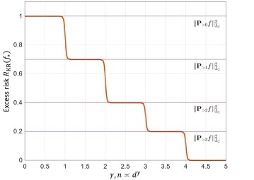
There are several recent works investigating the generalization error of kernel regression in the large-dimensional setting where . Ghorbani et al. (2021) considers the square-integrable function space on the sphere and proves that when is a non-integer, KRR is consistent if and only if the true function is a polynomial with a fixed degree . They also qualitatively reveal that the excess risk exhibits a periodic plateau behavior (Figure 1). Liu et al. (2021) considers the setting and assumes source condition to be . They give an upper bound of the generalization error with respect to bias and variance. Using this upper bound, they demonstrate that there could be multiple shapes of the generalization curve as the sample size increases. A more recent work Lu et al. (2023) studies early stopping kernel gradient flow in the large-dimensional setting . Assuming and considering the inner product kernel on the sphere , they prove an upper bound of the convergence rate and show the minimax optimality of early stopping kernel gradient flow. Interestingly, their results indicate that the minimax rate of the kernel regression for exhibits the similar periodic plateau phenomenon (Figure 1). This raises a natural and interesting question: is there a unified way to explain the periodic plateau behavior appeared in Lu et al. (2023) and Ghorbani et al. (2021)?
Suppose that is an RKHS associated with an inner product kernel defined on . The main focus of this paper aims to derive the matching upper and lower bounds of the generalization error and discuss the minimax optimality of KRR for general source condition , i.e., the true regression function . Allowing to vary is not only a more reasonable assumption for the true function, but also provides us a natural framework to clarify the relation between the results in Lu et al. (2023) and Ghorbani et al. (2020). In fact, a little bit interpolation space theory suggests that both the results in Ghorbani et al. (2021) and Lu et al. (2023) are two special cases of our results corresponding to and respectively. This paper has the following contributions:
-
•
We consider a more general framework than the traditional capacity-source condition. We introduce and in (4), which are key quantities depending on the RKHS, the true function and the regularization parameter . Under mild assumptions, we use these key quantities to express the matching upper and lower bounds of the generalization error as long as the regularization parameter satisfies some approximation conditions (Theorem 1). This framework makes few assumptions on the eigenvalues of the RKHS and the true function, thus enabling us to handle the large-dimensional setting and general source condition later. In the fixed-dimensional setting, our results in Theorem 1 also recovers the state-of-the-art theoretical results about the exact convergence rates of KRR in Li et al. (2023c).
-
•
We then add source condition into our new framework and consider the inner product kernel on the sphere . When we derive exact convergence rates (both upper and lower bounds) of the generalization error under the best choice of regularization parameter for any source condition and almost all (Theorem 2 for and Theorem 3 for ). We will see that the curves of rate varying along show similar periodic plateau and multiple descent behavior as in Lu et al. (2023). Moreover, we will see that the shapes of curves vary with and are totally different when and , with even more intriguing results in the limiting case and .
-
•
For the inner product kernel on the sphere , we further derive the corresponding minimax lower bound for all and . When , the exact rates in Theorem 3 match the minimax lower bound, and thus we prove the minimax optimality of KRR. When , the KRR is not minimax optimal, i.e., we discover a new version of the saturation effect of KRR. In the fixed-dimensional setting, the saturation effect of KRR only happens when . In the large-dimensional setting, we prove that a similar phenomenon also happens for . Specifically, for any , there will be corresponding ranges of such that the convergence rates of KRR can not achieve the minimax lower bound even under the best choice of regularization parameter.
1.1 Related work
In the introduction, we have mentioned several interesting topics about the KRR’s generalization behavior. These topics have been well-studied in the fixed-dimensional setting. The first essential question is the minimax optimality of KRR. Under the framework of capacity condition and source condition (), Caponnetto and de Vito (2007) proves the minimax optimality of KRR when . Then, extensive literature (see, e.g., Steinwart et al. 2009; Lin et al. 2018; Fischer and Steinwart 2020; Zhang et al. 2023a, b and the reference therein) studies the mis-specified case (), where Zhang et al. (2023a) proves the minimax optimality for all under further embedding index condition. The second question is the saturation effect of KRR when , which is conjectured by Bauer et al. (2007); Gerfo et al. (2008) and rigorously proved by Li et al. (2023b). Thirdly, due to the fantastic performance of overparameterized neural networks, the generalization ability of kernel interpolation has also raised a lot of interest. The results in Rakhlin and Zhai (2019); Buchholz (2022); Beaglehole et al. (2023); Li et al. (2023a) imply that kernel interpolation can not generalize in fixed-dimensional setting. Last but not least, Bordelon et al. (2020); Cui et al. (2021); Li et al. (2023c) study the learning curve of KRR, i.e., the exact generalization error (or exact order) for any regularization parameter .
In the large-dimensional setting, the answers to the above questions are not clear yet. Many researchers have studied these problems from different angles and settings. A line of work uses the tools of high-dimensional kernel random matrix approximation from Karoui (2010) and studies the generalization ability of kernel interpolation (Liang and Rakhlin, 2020; Liang et al., 2020). When , Liang and Rakhlin (2020) gives an upper bound of the generalization error of kernel interpolation and claims that the upper bound tends to 0 when the data exhibits a low-dimensional structure. Further, when , Liang et al. (2020) gives an upper bound with a specific convergence rate, which implies that kernel interpolation can generalize if and only if is not an integer. One closely related topic is the benign overfitting phenomenon, which we refer to Bartlett et al. (2020); Hastie et al. (2022); Muthukumar et al. (2020); Tsigler and Bartlett (2023).
Another line of work follows Ghorbani et al. (2021), which has been mentioned in the introduction. This line of work adopts the square-integrable assumption of the true function and aims to obtain the exact generalization error of kernel methods in various settings (Ghorbani et al., 2020; Mei et al., 2022; Mei and Montanari, 2022; Ghosh et al., 2021; Xiao et al., 2022; Hu and Lu, 2022; Misiakiewicz, 2022; Donhauser et al., 2021). To our knowledge, Lu et al. (2023) is the only literature that provides the minimax optimality result for specific kernel methods. As discussed in the introduction, Lu et al. (2023) considers the case () and kernel early stopping gradient flow. We will provide a detailed discussion on Lu et al. (2023) and Ghorbani et al. (2021) in Section 4. If we follow the line of research in the fixed-dimensional setting, considering general source condition and studying the minimax optimality (saturation effect) of KRR are essential steps to understand KRR’s generalization behavior in the large-dimensional setting.
2 Preliminaries
Let a compact set be the input space and be the output space. Let be an unknown probability distribution on satisfying and denote the corresponding marginal distribution on as . We use (in short ) to represent the -spaces. Throughout the paper, we make the following assumption:
Assumption 1
Suppose that is a separable RKHS on with respect to a continuous kernel function satisfying
where is an absolute constant.
Since we allow the dimension to diverge to infinity as , the RKHS may vary with and we suppose that Assumption 1 holds uniformly for all . For brevity of notations, we frequently omit the index in the rest of this paper.
Suppose that the samples are i.i.d. sampled from . Kernel ridge regression (KRR) constructs an estimator by solving the penalized least square problem
where is referred to as the regularization parameter.
Denote the samples as and . The representer theorem (see, e.g., Steinwart and Christmann 2008) gives an explicit expression of the KRR estimator, i.e.,
| (1) |
where
Denote the conditional mean:
We are interested in the convergence rates of the generalization error (excess risk) of :
Notations. We use asymptotic notations and . We also write for ; for ; for ; for . We will also use the probability versions of the asymptotic notations such as . For instance, we say the random variables satisfying if and only if for any , there exist a constant and such that .
2.1 Integral operator and interpolation space
Denote the natural embedding inclusion operator as . Then its adjoint operator is an integral operator, i.e., for and , we have
Under Assumption 1, and are Hilbert-Schmidt operators (thus compact) and the HS norms (denoted as ) satisfy that
Next, we can define two integral operators:
| (2) |
and are self-adjoint, positive-definite and trace class (thus Hilbert-Schmidt and compact) and the trace norms (denoted as ) satisfy that
The spectral theorem for self-adjoint compact operators yields that there is an at most countable index set , a non-increasing summable sequence and a family , such that is an orthonormal basis (ONB) of and is an ONB of . Further, the integral operators can be written as
We refer to and as the eigenfunctions and eigenvalues. The celebrated Mercer’s theorem (see, e.g., Steinwart and Christmann 2008, Theorem 4.49) shows that
where the convergence is absolute and uniform for .
Since we are going to consider the source condition in this paper, we need to introduce the interpolation spaces (power spaces) of RKHS. For any , the fractional power integral operator is defined as
Then the interpolation space (power space) is defined as
| (3) |
equipped with the inner product
It is easy to show that is also a separable Hilbert space with orthogonal basis . Specially, we have and . For , the embeddings exist and are compact (Fischer and Steinwart, 2020). For the functions in with larger , we say they have higher regularity (smoothness) with respect to the RKHS.
In the following of this paper, we assume . Also note that and are dependent on , thus are dependent on .
3 Main results
3.1 KRR’s generalization error in the general case
In this subsection, we consider a general framework for studying the generalization error of KRR, where we make quite mild assumptions on the RKHS and the true function . Note that in this framework, we allow to diverge to infinity as sample size and allow to change with . Therefore, the results in this subsection are applicable in the large-dimensional setting .
Given the RKHS and denote the true function as . We define the following important quantities:
| (4) | ||||
Assumption 2
Suppose that for some absolute constant ,
Assumption 2 assumes that the noise is non-vanishing and it holds for common nonparametric regression model where is an independent non-zero noise.
Assumption 3
Suppose that
| (5) |
and
| (6) |
In fact, it is allowed to multiply an absolute constant on the right sides of (5) and (6). Without loss of generality, we consider the constant to be .
Assumption 3 naturally holds for RKHSs with uniformly bounded eigenfunctions, i.e., . One can also show that RKHSs associated with inner product kernel on the sphere with uniform distribution satisfy Assumption 3 (see Lemma 20).
Now we begin to state the first important theorem in this paper.
Theorem 1
Note that the notation represents the limit as and we allow to diverge to infinity with . Theorem 1 provides the matching upper and lower bounds (8) for all satisfying the approximation conditions (7). Generally speaking, the conditions in (7) are more likely to hold for larger . For instance, we will show in the proof of Theorem 2 that if the conditions in (7) hold for for some , then they hold for all .
Basically, in (8), the term corresponds to the variance and corresponds to the bias. An obvious relation is , thus the first approximation condition in (7) guarantees that is not that small and the variance term tends to 0. In addition, if we take the traditional source condition assumption, i.e., for some constant and , easy calculation shows that for some constant only depending on and the constant in Assumption 1. This implies that the bias term tends to 0 as .
Under the capacity-source condition framework in the fixed-dimensional setting (as discussed in the introduction), Theorem 1 also recovers the state-of-the-art results in Li et al. (2023c). We emphasize that proving such tight bounds of the generalization error in the large-dimensional setting is nontrivial. In addition, the original bounds of the key quantities in (4) under the capacity-source condition framework are no longer sufficient in the large-dimensional setting. Given the information about the kernel and the true function, detailed calculations of and will be needed (see, e.g., Appendix B.2 for inner product kernel on the sphere).
3.2 Applications to inner product kernel on the sphere
In this subsection, we consider the inner product kernel on the sphere with uniform distribution. In the large-dimensional setting and under further source condition assumption, we apply Theorem 1 to prove the exact convergence rates of the generalization error of the KRR estimator. Then, we derive the corresponding minimax lower bound, which enables us to discuss the minimax optimality and the saturation effect of KRR.
Suppose that and is the uniform distribution on . We consider the inner product kernel, i.e., there exists a function such that . Then Mercer’s decomposition for the inner product kernel is given in the basis of spherical harmonics:
where are spherical harmonic polynomials of degree ; are the eigenvalues with multiplicity ; .
Assumption 4 (Inner product kernel)
Suppose that satisfies
where is a fixed function independent of and
Assumption 4 formally defines the kernel considered in this subsection. The purpose of assuming all the coefficients to be positive is to keep the main results and proofs clean. In fact, the proof is similar for other inner product kernels as long as we know which coefficients are positive, for instance, the neural tangent kernel in the following subsection. We assume (or ) to be fixed and we will ignore the dependence of constants on it in the rest of our paper.
The inner product kernel has attracted a lot of research (Liang et al., 2020; Ghorbani et al., 2021; Misiakiewicz, 2022; Xiao et al., 2022; Lu et al., 2023, etc.) and we have a concise characterization of and , which enables us to calculate the exact convergence rates of the key quantities in (4). We refer to Lemma 17, 18 and 19 in Appendix B.1 for details about and . The extension to general kernel can be extremely complicated and existing results also only consider the case where is the sphere (as this paper) or discrete hypercube (see, e.g., Mei et al. 2022; Aerni et al. 2022).
In the next assumption, we formally introduce the source condition, which characterizes the relative smoothness of with respect to .
Assumption 5 (Source condition)
-
(a)
Suppose that for some and satisfies that,
(9) where is a constant only depending on .
-
(b)
Denote as the smallest integer such that and . Define as the index set satisfying . Further suppose that there exists an absolute constant such that for any and with , we have
(10)
Assumption 5 (a) is usually used as the traditional source condition (Caponnetto, 2006; Fischer and Steinwart, 2020, etc.). In order to obtain a reasonable lower bound, we need Assumption 5 (b). It is equivalent to assume that the norm of the projection of on the first -th eigenspace is non-vanishing. Similar assumptions have been adopted when one interested in the lower bound of generalization error in the fixed-dimensional setting, e.g., Eq.(8) in Cui et al. (2021) and Assumption 3 in Li et al. (2023c). In a word, recalling definition 3, Assumption 5 implies that and for any .
Now we are ready to state two theorems about the exact convergence rates of the generalization error of KRR, which deal with two different ranges of source condition: and .
Theorem 2 (Exact convergence rates when )
Let for some fixed and absolute constants . Consider and the marginal distribution to be the uniform distribution. Let be a sequence of inner product kernels on the sphere satisfying Assumption 1 and 4. Further suppose that Assumption 2 holds and Assumption 5 holds for some . Let be the KRR estimator defined by (1). Define , then we have:
-
(i)
When for some , by choosing , we have
(11) -
(ii)
When for some , by choosing , we have
(12) -
(iii)
When for some , by choosing , we have
(13)
The notation involves constants only depending on and . In addition, the convergence rates of the generalization error of KRR can not be faster than above for any choice of regularization parameter .
Theorem 3 (Exact convergence rates when )
Let for some fixed and absolute constants . Consider and the marginal distribution to be the uniform distribution. Let be a sequence of inner product kernels on the sphere satisfying Assumption 1 and 4. Further suppose that Assumption 2 holds and Assumption 5 holds for some . Let be the KRR estimator defined by (1). Then we have:
-
•
If :
-
(i)
When for some , by choosing , we have
(14) -
(ii)
When for some , by choosing , we have
(15)
The notation involves constants only depending on and .
-
(i)
-
•
If : we have the same convergence rates as the case for those
Remark 4
For technical reasons, when , we only prove the convergence rates for those . Note that we have when ; and when . Therefore, we have actually proved for almost all .
Note that Theorem 2 and Theorem 3 show exact convergence rates (both upper and lower bounds) of KRR’s generalization error, which is a much stronger result than only proving an upper bound. As we will see in Appendix B.4, since could be infinite when thus could be infinite, the proof of Theorem 3 requires a little more technique. In addition, we will prove in Theorem 5 that the rates in Theorem 3 () achieve the minimax lower bound. Together with the statement at the end of Theorem 2, we actually prove that the rates in Theorem 2 and Theorem 3 are the fastest convergence rates that KRR can achieve.
Next, we will state the minimax lower bound in the same large-dimensional and source condition setting as Theorem 2 and Theorem 3.
Theorem 5 (Minimax lower bound)
Let for some fixed and absolute constants . Consider and the marginal distribution to be the uniform distribution. Let be a sequence of inner product kernels on the sphere satisfying Assumption 1 and 4. Let consist of all the distributions on such that Assumption 2 holds and Assumption 5 holds for some . Then we have:
-
(i)
When for some , for any , there exist constants and only depending on and such that for any , we have:
(16) -
(ii)
When for some , there exist constants and only depending on and such that for any , we have:
(17)
Theorem 5 states that there is no estimator (or learning method) that can achieve faster convergence rates than (16) and (17).
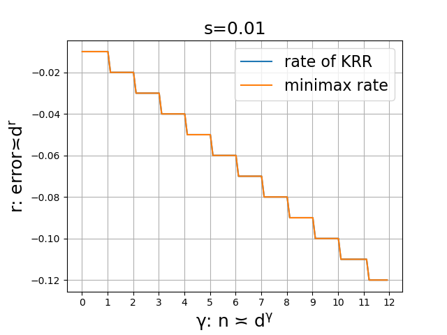
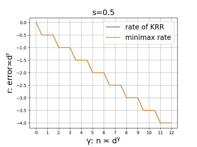
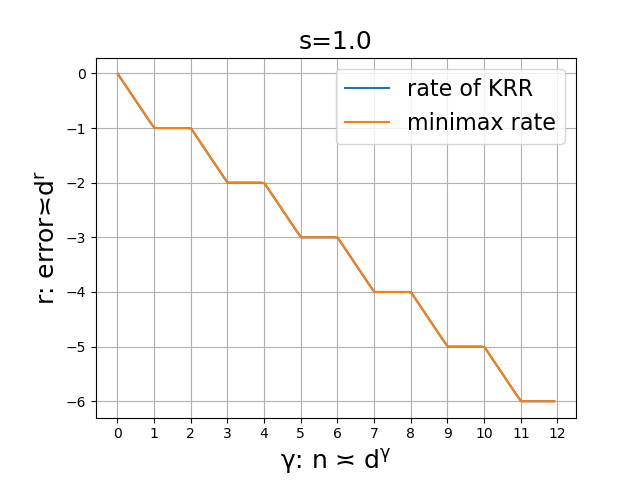
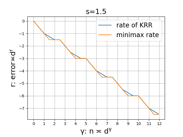
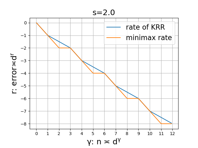
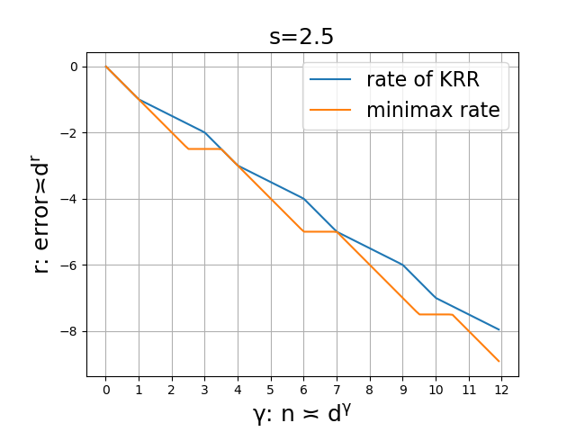
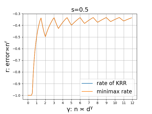
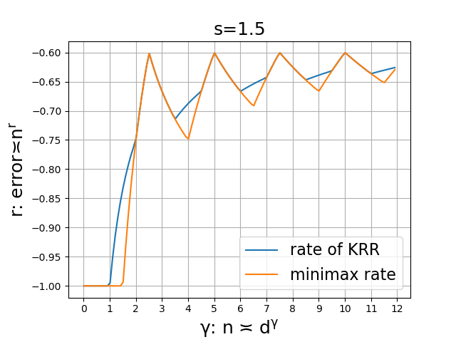
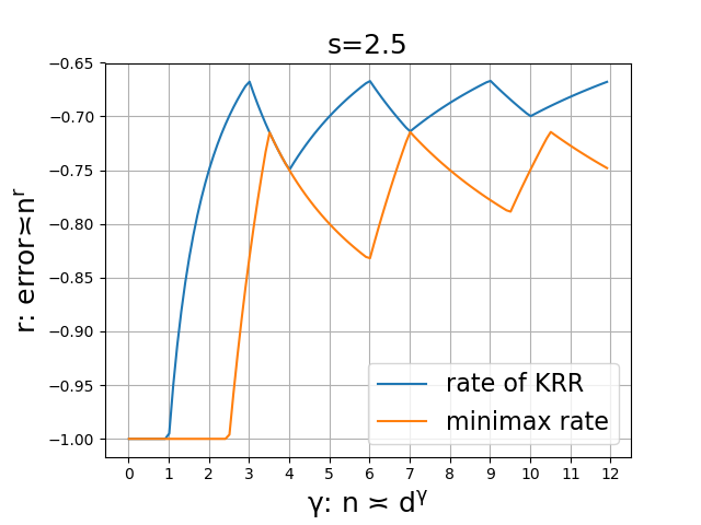
Summarizing the results in Theorem 2, Theorem 3 and Theorem 5, Figure 2 shows the convergence rates of KRR and corresponding minimax lower rates with respect to dimension for any . We can see that the rates decrease when the scaling increases, indicating that the performance becomes better when the sample size grows. Moreover, we can observe several intriguing phenomena.
Curve’s evolution with source condition. Since we consider source condition , we can compare the rate curves in Figure 2 for different and see how they evolve with .
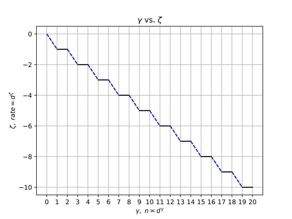
Let us first see the minimax lower rates. For any , there are 2 periods with respect to the value of : The length of the first period, i.e., , will decrease to 0 as getting close to 0; The length of the second period, i.e., , equals for all .
Next, we see the convergence rates of KRR, which is more intriguing.
-
•
When , there are 2 periods with respect to the value of and the curve is the same as the minimax lower rates. (In fact, Theorem 3 only proves the results for when , we write with a little bit of notation abusement.)
-
•
When , there are 3 periods with respect to the value of : The length of the first period, i.e., , equals 1 for all ; The length of the second period, i.e., is , thus this period will degenerate as getting close to 1; The length of the third period, i.e., is , thus this period will degenerate as getting close to 2.
-
•
When , the curve does not change with and there are 2 periods with respect to the value of : The length of the first period, i.e., , equals 1 for all ; The length of the second period, i.e., , equals 2 for all .
Minimax optimality and new saturation effect of KRR. As can be seen in Figure 2 (a)(b)(c), the convergence rates of KRR match the minimax lower bound for all , thus we prove the minimax optimality of KRR when . In contrast, when , Figure 2 (d)(e)(f) illustrate that KRR can not achieve the minimax lower bound in Theorem 5 for certain ranges of , which we refer to as the new saturation effect of KRR. We will discuss the implications of this new saturation effect in the following.
In the fixed-dimensional setting, kernel ridge regression has been studied as a special kind of spectral algorithm (Gerfo et al., 2008). Each spectral algorithm is determined by a filter function and the difference between spectral algorithms is characterized by an index called the “qualification” () of the filter function (see, e.g., Zhang et al. 2023a, Definition 1). Since KRR has qualification and gradient flow has qualification (Zhang et al., 2023a, Example 1, 2), the main difference between KRR and gradient flow is the saturation effect (Li et al., 2023b). It says when , no matter how carefully one tunes the KRR, the convergence rate can not be faster than , thus can not achieve the minimax lower bound .
In the large-dimensional setting and for inner product kernel on the sphere, our results show that the saturation effect of KRR happens in a new regime . In addition, we conjecture that there are other spectral algorithms (e.g., gradient flow) that can achieve the minimax lower bound in Theorem 5 for all . This new saturation effect strongly suggests that qualification () itself is insufficient to characterize the filter function (or spectral algorithm) in the large-dimensional setting.
Periodic plateau behavior. If , Figure 2 (a)(b)(c) show that when varies within certain ranges, the value of vertical axis, r, does not change. We refer to such ranges of as the plateau period. When exceeds 2, the plateau period of KRR’s convergence rates degenerates and the plateau period of minimax lower rates still exists. Also note that the length of each plateau period varies with the values .
For these plateau periods, if we fix a large dimension and increase (or equivalently, increase the sample size ), the convergence rates of KRR or minimax lower rates stay invariant in certain ranges. Therefore, in order to improve the rate, one has to increase the sample size above a certain threshold.
Figure 3 provides an alternative representation of our results, which shows the convergence rates of KRR and corresponding minimax lower rates with respect to sample size . We can observe the “multiple descent behavior” ( for both the convergence rates of KRR and the minimax lower rates) from Figure 3.
Multiple descent behavior. Let us first see the minimax lower rates. For any , the curve achieves its peaks at , and achieve its isolated valleys at .
For the convergence rates of KRR:
-
•
When , the curve is the same as the curve of minimax lower rates.
-
•
When , the curve achieves its peaks at ; achieve its isolated valleys at and achieve its hillside at .
-
•
When , the curve does not change with , which achieves its peaks at , and achieve its isolated valleys at .
3.3 Applications to neural tangent kernel
In this subsection, we look at a specific example, i.e., the neural tangent kernel (NTK) of a two-layer fully connected ReLU neural network . Still, we suppose that and is uniform distribution on . It has been shown in Bietti and Mairal (2019); Lu et al. (2023) that NTK is an example of inner product kernel satisfying
where is a fixed function independent of and
Lemma 5 in Lu et al. (2023) also showed that .
For the neural tangent kernel , the following theorems provide the exact convergence rates of the generalization error of KRR and the corresponding minimax lower bound. Since the proofs are similar to Theorem 2, Theorem 3 and Theorem 5, we omit the proofs of the following theorems.
Theorem 6 (NTK: exact convergence rates when )
Let for some fixed and absolute constants . Consider and the marginal distribution to be the uniform distribution. Let be a sequence of neural tangent kernels of a two-layer fully connected ReLU neural network on the sphere. Further suppose that Assumption 2 holds and Assumption 5 holds for some . Let be the KRR estimator defined by (1). For any , we define , if ; and define , if . Define , then we have:
-
(i)
When for some , by choosing , we have
(18) -
(ii)
When for some , by choosing , we have
(19) -
(iii)
When for some , by choosing , we have
(20)
The notation involves constants only depending on and .
Theorem 7 (NTK: exact convergence rates when )
Let for some fixed and absolute constants . Consider and the marginal distribution to be the uniform distribution. Let be a sequence of neural tangent kernels of a two-layer fully connected ReLU neural network on the sphere. Further suppose that Assumption 2 holds and Assumption 5 holds for some . Let be the KRR estimator defined by (1). Denote . For any , we define , if ; and define , if . Then we have:
-
•
If :
-
(i)
When for some , by choosing , we have
(21) -
(ii)
When for some , by choosing , we have
(22)
The notation involves constants only depending on and .
-
(i)
-
•
If : we have the same convergence rates as the case for those
Theorem 8 (NTK: minimax lower bound)
Let for some fixed and absolute constants . Consider and the marginal distribution to be the uniform distribution. Let be a sequence of neural tangent kernels of a two-layer fully connected ReLU neural network on the sphere. Let consist of all the distributions on such that Assumption 2 holds and Assumption 5 holds for some . Then we have:
-
(i)
When for some , for any , there exist constants and only depending on and such that for any , we have:
(23) -
(ii)
When for some , there exist constants and only depending on and such that for any , we have:
(24)
Note that the results in this subsection will be the same as the theorems in Section 3.2 if we change the above definition of to .
4 Conclusion and discussion
In this paper, we first establish a new framework for studying the asymptotic generalization error of kernel ridge regression (Theorem 1). This framework makes few assumptions on the RKHS, the true function and the relation between and , thus it is suitable for studying various topics about KRR’s generalization error in both fixed-dimensional and large-dimensional settings. Moreover, the results in Theorem 1 provides the matching upper and lower bounds of the generalization error with certain regularization parameter, which is more instructive than just the upper bound.
Based on this framework, we then consider inner product kernel on the sphere and the large-dimensional setting (). Given that falls into , an interpolation space of RKHS, Theorem 2 and Theorem 3 prove the exact convergence rates of KRR’s generalization error under the best choice of regularization parameter and Theorem 5 proves the corresponding minimax lower bound. These results show the minimax optimality of KRR when and the new saturation effect of KRR . We also discuss how the rate curves (varying along ) evolve with the value of and discuss the “periodic plateau behavior” and “multiple descent behavior” of KRR in the large-dimensional setting.
Similar periodic behavior has been observed for kernel methods in the large-dimensional setting in related literature, we next make some discussion on these works. There is a line of work studying the inconsistency of kernel methods with inner product kernels in the large-dimensional setting (Ghorbani et al., 2021; Mei et al., 2022; Misiakiewicz, 2022, etc.). Assuming the true function to be square-integrable (or equivalently in our setting) on the sphere, Ghorbani et al. (2021, Theorem 4) proves that the generalization error of KRR satisfies (with high probability)
| (25) |
where is the greatest integer that is less or equal to , means the projection onto polynomials with degree , is any positive real number and is defined as Ghorbani et al. 2021, Eq.(20). (25) implies that generalization error will drop when exceeds an integer and stay invariant for other (see the cartoon representation in Ghorbani et al. 2021, Figure 5). In our paper, when and efficiently close to 0, similar behavior has been observed in Figure 2 (a) that the convergence rate drops abruptly around each integer .
A more recent work Lu et al. (2023) considers the optimality of early stopping kernel gradient flow in the same large-dimensional setting . They also consider inner product kernel on the sphere and assume that the true function falls into the RKHS (or equivalently, ). Denoting , Lu et al. 2023, Theorem 4.3 proves that by properly choosing the early stopping time , the upper bound of the convergence rate is:
-
•
When , then, there exist constants and , where , only depending on , , and , such that for any , we have
(26) holds with probability at least .
-
•
When , for any , there exist constants and , where , only depending on , , , and , such that for any , we have
(27) holds with probability at least .
-
•
When , then, for any , there exist constants and , where , only depending on , , , and , such that for any , we have
(28) holds with probability at least .
Ignoring the log term, simple calculation shows that the convergence rate is consistent with the rate in Theorem 2 when (see, e.g., Figure 2 (c)). Lu et al. (2023) also proves that the above upper bound matches the minimax lower bound, thus proving the minimax optimality of early stopping kernel gradient flow under the assumption . In contrast to Lu et al. (2023), we provide not only the upper bound but also the lower bound of the convergence rates of KRR under general source condition . We have seen that the “periodic plateau behavior” and “multiple descent behavior” observed in Lu et al. (2023) still exist for and the plateau length will change with the value of . By considering source condition , our restriction on the true function is much milder, thus we provide a more complete characterization of the generalization error of KRR.
The periodic behavior in large dimension has also been observed for “kernel interpolation estimator”, for instance, Liang et al. (2020) for the inner product kernel and Aerni et al. (2022) for the convolutional kernel. Although technically complicated, a direct follow-up question is the convergence rate of generalization error for general kernels and domains. We believe that it is an interesting research direction to study the generalization behavior of kernel methods in the large-dimensional setting, which will exhibit a wealth of new phenomena compared with the fixed-dimensional setting.
Acknowledgments and Disclosure of Funding
Qian Lin is supported in part by National Natural Science Foundation of China (Grant 92370122, Grant 11971257) and the Beijing Natural Science Foundation (Grant Z190001).
Appendix
Appendix A Proof of Theorem 1
The proof of Theorem 1 consists of the following steps: First, we introduce the bias-variance decomposition in Section A.1. Next, we derive the bounds of variance term in Section A.2 and bias term in Section A.3. Finally, using the results in these sections, we formally prove Theorem 1 in Section A.4.
A.1 Bias-variance decomposition
The proof of Theorem 1 is based on the traditional bias-variance decomposition. The contribution in this paper is that we refine the tools in Li et al. (2023a) and Li et al. (2023c) to handle the large-dimensional case. Throughout the proof, we denote
| (29) |
where is the regularization parameter. We use to denote the operator norm of a bounded linear operator from a Banach space to , i.e., . Without bringing ambiguity, we will briefly denote the operator norm as . In addition, we use and to denote the trace and the trace norm of an operator. We use to denote the Hilbert-Schmidt norm. In addition, we denote as , as for brevity throughout the proof.
We also need the following essential notations in our proof, which are frequently used in related literature. Denote the samples . Define the sampling operator and its adjoint operator . Then we can define . Further, we define the sample covariance operator as
| (30) |
Then we know that and is a trace class thus compact operator. Further, define the sample basis function
| (31) |
As shown in Caponnetto and de Vito (2007), the operator form of the KRR estimator (1) writes
| (32) |
In order to derive the bias term, we define
| (33) |
and
| (34) |
We also need to define the expectation of as
| (35) |
and
| (36) |
Then we have the decomposition
| (37) |
Taking expectation over the noise conditioned on and noticing that are independent noise with mean 0 and variance , we obtain the bias-variance decomposition:
| (38) |
where
| (39) |
Given the decomposition (38), we next derive the upper and lower bounds of and in the following two subsections.
A.2 Variance term
In this subsection, our goal is to derive Theorem 13, which shows the upper and lower bounds of variance under some approximation conditions. Before formally introduce Theorem 13, we have a lot of preparatory work.
Following Li et al. (2023a), we consider the sample subspace
Recall the notation and . Define the normalized sample kernel matrix
Then, it is easy to verify that and is the representation matrix of under the natural basis . Consequently, for any continuous function we have
| (40) |
where the left-hand side means applying the operator elementwise. Since the property of reproducing kernel Hilbert space implies , taking inner product elementwise between (40) and , we have
| (41) |
Moreover, for , we define empirical semi-inner product
| (42) |
and denote by the corresponding empirical semi-norm. We also denote by the empirical measure with respect to .
For simplicity of notations, we denote , in the rest of the proof. The following lemma rewrites the variance term (39) using the empirical semi-norm.
Lemma 9
The variance term in (39) satisfies that
| (43) |
Proof First, we have
| (44) |
Next, using (41) and the fact that , we have
which implies
| (45) |
Therefore, plugging (A.2) into (A.2), we get the desired results
The operator form (43) allows us to apply concentration inequalities and establish the following two-step approximation (recall the notations and in (29)).
| (46) |
Note that the above two-step approximation is an enhanced version of approximation (S24) in Li et al. (2023a).
Approximation B. The following lemma characterizes the magnitude of Approximation B in high probability. Recall the definitions of and in (4).
Lemma 10 (Approximation B)
Proof Define a function
| (49) |
Since Assumption 3 holds, we have
Applying Proposition 34 for and noticing that , we have
| (50) |
with probability at least .
Approximation A. The proof of Approximation A requires the following proposition, which is a simple but important observation by Li et al. (2023b).
Proposition 11
For any , we have
| (51) |
Proof Notice that , and thus
The second inequality comes from the definition of .
The following lemma characterizes the magnitude of Approximation A in high probability.
Lemma 12 (Approximation A)
Proof First, we rewrite as
| (54) |
where for the second line, we use Proposition 11 to transfer norms into .
Given the notations of in (A.2) (both are functions of and ), we begin to handle :
| (55) |
Now we bound the third term in (A.2). Denote , using Lemma 38, we have
We use to denote that is a positive semi-definite operator. Using the fact that for a self-adjoint operator , we have
In addition, Lemma 38 shows that . So we have
Define an operator , we have
Using Lemma 35 to , , for any fixed , with probability at least , we have
where
Further recall that the condition implies that and thus , so when is sufficiently large, we can conclude that
| (56) |
Next we bound the forth term in (A.2). Using Lemma 37, we have
| (57) |
Finally, we bound the first two terms in (A.2). Since we have assumed , (56) implies that when is sufficiently large, we have
Therefore, we have
| (58) |
and
| (59) |
Plugging (56), (57), (A.2) and (A.2), into (A.2), when is sufficiently large, with probability at least , we have
| (60) |
Further, when is sufficiently large, with probability at least , we also have
| (61) |
where the third line follows from Lemma 10.
Now we are ready to derive the upper bound of . Combining the bound (60) and (A.2), when is sufficiently large, with probability at least , we have
| (62) |
Without loss of generality, we can assume (A.2) holds with probability at least and we finish the proof.
Final proof of the variance term. Now we are ready to state the theorem about the variance term.
Theorem 13 (Variance term)
Proof Lemma 9 has shown that
Denote as in Lemma 12, then conditions (63) and Lemma 12 imply that
Further recall that in Lemma 10, we have defined
Then on the one hand, Lemma 10 shows that, for any , when is sufficiently large, with probability at least , we have
which further implies
| (65) |
On the other hand, we also have
which further implies
| (66) |
A.3 Bias term
In this subsection, our goal is to derive Theorem 16, which shows the upper and lower bounds of bias under some approximation conditions.
The following lemma characterizes the dominant term of .
Proof Recall that we have defined and . Therefore, we have
Our next goal is to prove that second term in (67) is higher order infinitesimal, i.e., .
Lemma 15
Proof To begin with, be definition, we rewrite (68) as follows
| (71) |
For any and , suppose that satisfying that . So for the first term in (A.3), we have
| (72) |
For the second term, since we have assumed , for any fixed , when is sufficiently large, we have proved in (A.2) and (A.2) that, with probability at least
| (73) |
For the third term in (A.3), it can be rewritten as
| (74) |
Denote . To use Bernstein inequality, we need to bound the -th moment of :
| (75) |
Note that Lemma 37 shows that
By definition of , we also have
| (76) |
In addition, we have proved in Lemma 14 that
So we get the upper bound of (A.3), i.e.,
Using Lemma 36 with therein notations: and , for any fixed , with probability at least , we have
| (77) |
Since we have assumed and , (77) further implies
| (78) |
Plugging (A.3), (73) and (78) into (A.3), we finish the proof.
Final proof of the bias term. Now we are ready to state the theorem about the bias term.
Theorem 16
A.4 Final proof of Theorem 1
Now we are ready to prove Theorem 1. Note that we have assumed in Theorem 1 that satisfies all the conditions required in Theorem 13 and Theorem 16. Therefore, Theorem 13 and Theorem 16 show that
Recalling the bias-variance decomposition (38), we finish the proof.
Appendix B Proof of inner product kernel
In this section, we aim to apply Theorem 1 to prove the results in Section 3.2. We will see that the application is nontrivial and is an important contribution of this paper.
We first introduce more necessary preliminaries in Appendix B.1, which is an preparation for subsequent calculations. Next, in order to apply Theorem 1 to get specific convergence rates, we calculate the exact convergence rates of the key quantities therein in Appendix B.2. Finally, we state the proof of Theorem 2 and Theorem 3 in turn in Appendix B.3 and B.4. We will see that there are essential differences in the proof of these two theorems.
B.1 More preliminaries about inner product kernel on the sphere
Suppose that and is the uniform distribution on . Recall that in Section 3.2, we consider the inner product kernel, i.e., there exists a function such that . Then Mercer’s decomposition for the inner product kernel is given in the basis of spherical harmonics:
| (81) |
where are spherical harmonic polynomials of degree ; are the eigenvalues with multiplicity ; .
By known results on spherical harmonics, the eigenvalues ’s have the following explicit expression (Bietti and Mairal, 2019):
| (82) |
where is the -th Legendre polynomial in dimension , denotes the surface of the sphere .
Although the above expression of are complicated, Lemma 17 19 (mainly cited from Lu et al. 2023) give concise characterizations of and , which is sufficient for the analysis in this paper.
Lemma 17
Proof From equation (22) in Ghorbani et al. (2021), for any integer , there exist constants only depending on and , such that for any , we have
| (84) |
Note that for any , we have .
Therefore, letting and , then we finish the proof.
The following property of the eigenvalues indicates that when we consider with any fixed , the subsequent eigenvalues ’s () are much smaller than . The following lemma is the same as Lemma 3.3 in Lu et al. (2023).
Lemma 18
Lemma 19
For an integer , denote as the multiplicity of the eigenspace corresponding to in the Mercer’s decomposition. For any fixed integer , there exist constants and only depending on , such that for any , we have
| (85) |
Proof When , we have , which satisfies (85). When , Section 1.6 in Gallier et al. (2020) shows that
Note that is fixed and we consider those , (85) follows from detailed calculations using Stirling’s approximation. We refer to Lemma B.1 and Lemma D.4 in Lu et al. (2023) for more details.
The following lemma verifies that if we consider the inner product kernel on the sphere, then Assumption 3 naturally holds.
Lemma 20
Suppose that and is the uniform distribution on . Suppose that is an inner product kernel, then Assumption 3 holds.
B.2 Calculations of some key quantities
Based on the information of the eigenvalues in the last subsection, this subsection determines the exact convergence rates of the quantities appeared in Theorem 1. These rates will finally determine the convergence rates in Theorem 2 and Theorem 3. Note that we assume diverges to infinite with in Theorem 2 and Theorem 3 .
Lemma 21
Proof If for some , Lemma 17 and Lemma 19 show that there exist constants and only depending on (recall that we ignore the dependence on ), such that for any , we have
| (88) |
and for ,
| (89) |
We first prove (86). On the one hand, for any , we have
| (90) |
where we use the fact that for the third inequality.
On the other hand, for any , we have
| (91) |
Now we begin to prove (87). On the one hand, for any we have
| (92) |
Note that for the forth equation, we use the fact that (when d is sufficiently large), which can be proved by Lemma 18.
On the other hand, for any , we have
| (93) |
Before stating lemmas about , we first introduce the following useful lemma.
Lemma 22
Consider and the marginal distribution to be the uniform distribution. Let be a sequence of inner product kernels on the sphere satisfying Assumption 1 and 4. Further suppose that Assumption 5 holds for some . Suppose that are two real numbers such that
| (94) |
Then by choosing for some , if for some , we have
| (95) |
The notation involves constants only depending on and , where and are the constants from Assumption 5.
Proof Similar as the proof of Lemma 21, if for some , there exist constants and only depending on , such that for any , we have
| (96) |
and for ,
| (97) |
On the one hand, since (94) holds, for any , we have
| (98) |
Note that Assumption 5 (a) implies ; We also use the fact that , which can be proved by Lemma 18.
On the other hand, for any , we have
| (99) |
We use Assumption 5 (b), i.e., and , to obtain the lower bound. Combining (B.2) and (B.2), we finish the proof.
Lemma 23
Consider and the marginal distribution to be the uniform distribution. Let be a sequence of inner product kernels on the sphere satisfying Assumption 1 and 4. Further suppose that Assumption 5 holds for some . Define . By choosing for some , we have: if for some , we have
| (100) |
The notation involves constants only depending on and , where and are the constants from Assumption 5.
Proof When , can be viewed as in Lemma 22 with . The conditions (94) are satisfied and Lemma 22 shows that
| (101) |
When , without loss of generality, we can assume and . Recall we have proved in Lemma 17 that remains as a constant as . On the one hand, Assumption 5 (b) also implies without loss of generality, which further implies
| (102) |
On the other hand, since , we have
| (103) |
Further note that since and , (102) and (B.2) implies
We finish the proof.
The following lemma applies for those , which gives an upper bound of .
Lemma 24
Consider and the marginal distribution to be the uniform distribution. Let be a sequence of inner product kernels on the sphere satisfying Assumption 1 and 4. Further suppose that Assumption 5 holds for some . Define . By choosing for some , we have: if for some , we have
| (104) |
The notation involves constants only depending on and , where is the constant from Assumption 5.
Proof First, Cauchy-Schwarz inequality shows that
| (105) |
When , defined above can be viewed as in Lemma 22 with . In addition, the conditions (94) are satisfied, thus Lemma 22 shows that
| (106) |
Since we assume the kernel to be bounded in Assumption 1, we can assume and without loss of generality. When , on the one hand, Assumption 5 (b) also implies
| (107) |
On the other hand, since , we have
| (108) |
Further note that since and , (107) and (B.2) implies
Therefore, we have for any .
When , the following lemma gives an upper bound of .
Lemma 25
Consider and the marginal distribution to be the uniform distribution. Let be a sequence of inner product kernels on the sphere satisfying Assumption 1 and 4. Further suppose that Assumption 5 holds for some . Recall the definition of in (36). By choosing for some , we have: if for some , we have
| (109) |
The notation involves constants only depending on and , where is the constant from Assumption 5.
B.3 Proof of Theorem 2
In the last subsection, we have calculated the exact convergence rates of when for some . Note that we have proved in Lemma 20 that Assumption 3 naturally holds for inner product kernel on the sphere. Now we are ready to apply Theorem 1 to prove Theorem 2. The proof mainly consists of 3 steps:
- (1)
- (2)
-
(3)
Using the monotonicity of with respect to , we demonstrate that is the best choice of regularization parameter, i.e., the generalization error of KRR estimator is the smallest when . That is to say, the convergence rate of the generalization error can not be faster than the rate when choosing .
Note that we expect and . Step 1 actually indicates the regularization such that the bias and variance are balanced. Together with Theorem 13 and 16, Step 2 further verifies that and indeed hold for those . Thus they are indeed balanced under the choice of .
Final proof of Theorem 2. In the following of the proof, we omit the dependence of constants on and .
Step 1:
Note that we assume in this theorem and . For specific range of , we discuss the range of . Recall that we define .
- •
- •
- •
Step 2: In order to apply Theorem 13 and Theorem 16 so that we know the exact convergence rates of and , we first check the approximation conditions (63) and (69), or equivalently conditions (7), hold for . Recall that we have calculated the convergence rates of and in Lemma 21 and Lemma 24.
-
•
When : recall that .
The first condition in (7) is equivalent to
which naturally holds for all .
The second condition in (7) is equivalent towhich naturally holds for all and . When , we actually need to choose and the second condition will hold.
The third condition in (7) is equivalent towhich naturally holds for all and . In addition, one can also check that the third condition in (7) holds when and .
-
•
When : recall that .
-
•
When : recall that .
Up to now, we have verified conditions (7) for . Furthermore, simple calculation shows that the order of
| (117) |
are all non-decreasing with respect to , where we choose . Therefore, the above results indicate that conditions (7) holds for all .
Step 3:
In step 2, on the one hand, we prove that by choosing ,
| (118) |
On the other hand, we also prove that by choosing ,
| (119) |
In the following, we handle those . Recall that we have shown in the proof of Lemma 9 that
One simple but critical observation from Li et al. (2023b) is that
where represents the partial order of positive semi-definite matrices, and thus for , we have
Also note that by the definition of , we actually have
| (120) |
Therefore, for those , we have
| (121) |
To sum up, (118), (119) and (121) show that by choosing as in step 1, we obtain the convergence rates of KRR estimator under the best regularization. Using Lemma 23 to calculate the rate of , we finish the proof.
B.4 Proof of Theorem 3
Recall that in the proof of Theorem 16, we use to bound and show that . Unfortunately, the calculation of in Lemma 24 only holds for and it could be infinite when . Extensive literature then assume to be bounded and use to bound . When the dimension is fixed, Zhang et al. (2023a) first use a truncation method together with the -embedding property of to remove the boundedness assumption when . We will see in the proof of Theorem 3 that this technique still works in the large-dimensional setting.
To be specific, when we further assume , we have the following Theorem which is a refined version of Lemma 15.
Lemma 26
Proof Recall the decomposition (A.3) in the proof of Lemma 15. The first two terms in (A.3) can be handled without any difference. Our goal here is to prove the following equation and we will finish the proof:
| (125) |
Similar as (A.3), we rewrite the left hand side of (125) as
| (126) |
Denote . Further consider the subset and , where will be chosen appropriately later. Decompose as and we have the following decomposition of (126):
| (127) |
Next we choose such that
| (128) |
where is given in (123). Then we can bound the three terms in (B.4) as follows:
For the first term in (B.4), denoted as I, notice that
| (129) |
Imitating the procedure in the proof of Lemma 15 and using (122), (123), we have
| (130) |
For the second term in (B.4), denoted as II. Since , Lemma 42 shows that,
| (131) |
with embedding norm less than a constant . Then Assumption 5 (a) implies that there exists only depending on and such that . Using the Markov inequality, we have
Further, since (128) guarantees , we have
| (132) |
For the third term in (B.4), denoted as III. Since Lemma 37 implies that so
| III | ||||
| (133) |
where we use Cauchy-Schwarz inequality for the third inequality and (14) for the forth inequality. Recalling that the choices of satisfy and we have assumed , we have
| (134) |
Plugging (130), (B.4) and (134) into (B.4), we finish the proof.
Based on Lemma 26 and Lemma 14, we have the following theorem about the exact rate of bias term when .
Theorem 27
Proof The triangle inequality implies that
When satisfies (135) and (136), Lemma 14 and Lemma 26 prove that
which directly prove (137).
Now we are ready to prove Theorem 3. Since we do not claim that the regularization choice in Theorem 3 is the best, we only need the first two steps in the proof of Theorem 2.
Final proof of Theorem 3. In the following of the proof, we omit the dependence of constants on and .
Step 1:
Note that we assume in this theorem and . For specific range of , we discuss the range of .
- •
- •
- •
Note that the present result is different from the result of the Step 1 in the proof of Theorem (2). There are only two intervals of , i.e.,
It is worth mentioning that in the second interval of , we can actually choose and we have
| (143) |
That is to say, we can choose smaller and the rate of will remain unchanged. We have shown in (117) and the discussion below it that the approximation conditions are easier to satisfied for smaller . Therefore, in the following of the proof, we define
| (144) |
and verify the approximation conditions for . For consistency of notation, we also define
| (145) |
Step 2:
In order to apply Theorem 13 and Theorem 27 so that we know the exact convergence rates of and , we first check the approximation conditions (63), (135) and (136) hold for . We first list all the approximation conditions below:
| (146) | ||||
Recall that we have calculated the convergence rates of and in Lemma 21 and Lemma 25.
-
•
When : recall that .
The first condition in (146) is equivalent to
which naturally holds for all .
The second condition in (146) is equivalent towhich naturally holds for all and . When , we actually need to choose and the second condition will hold.
The third condition in (146) is equivalent towhich naturally holds for all and . In addition, one can also check that the third condition in (146) holds when and .
The forth condition in (146) is equivalent to(147) If , (147) naturally holds for all and . In addition, one can also check that the forth condition in (146) holds when and .
If , (147) only holds for and . That is to say, we can not verify (147) holds for(148) -
•
When : recall that .
The first condition in (146) is equivalent to
which naturally holds for all .
The second condition in (146) is equivalent towhich naturally holds for all .
The third condition in (146) is equivalent towhich naturally holds for all .
The forth condition in (146) is equivalent to(149) If , (149) naturally holds for all and . In addition, one can also check that the forth condition in (146) holds when and .
If , (149) only holds for and . That is to say, we can not verify (147) holds for(150)
Up to now, we have verified the approximation conditions (146) for
| (151) |
and
| (152) |
Using Lemma 23 to calculate the rate of , we finish the proof.
Appendix C Proof of Minimax lower bound
C.1 More preliminaries about minimax lower bound
Let’s first introduce several concepts about minimax lower bound which can be frequently found in related literature Yang and Barron (1999); Lu et al. (2023), etc..
Suppose that is a topological space with a compatible loss function , which are mappings from to with and for . We call such a loss function a distance. We introduce the packing entropy and covering entropy below:
Definition 28 (Packing entropy)
A finite set is said to be an -packing set in with separation , if for any , we have . The logarithm of the maximum cardinality of -packing set is called the -packing entropy or Kolmogorov capacity of with distance and is denoted by .
Definition 29 (Covering entropy)
A set is said to be an -net for if for any , there exists an such that . The logarithm of the minimum cardinality of -net is called the -covering entropy of and is denoted by .
Let , where is the constant from Assumption 5. Without loss of generality, we can consider be the unit ball in . Let be the -packing entropy of and be the -covering entropy of . Recalling that is the marginal distribution on we further define
and let be the -covering entropy of . It is easy to see that is an subset of which is defined in Theorem 5, i.e., .
The following lemmas give useful characterizations of and . We refer to Lemma A.5, Lemma A.7 and Lemma A.8 in Lu et al. (2023) for their proofs.
Lemma 30
For any , we have
Lemma 31
.
Lemma 32
Let be the eigenvalues of . For any , let . We have
| (153) |
The following important lemma is a modification of Theorem 1 and Corollary 1 in Yang and Barron (1999). We refer to Lemma 4.1 in Lu et al. (2023) for the proof.
Lemma 33
Let be a constant only depending on , , and , where are the constants given in Theorem 5. For any only depending on , , , , , and and satisfying
| (154) |
we have
| (155) |
C.2 Proof of Theorem 5
Now we are ready to use the lemmas in the last subsection to prove Theorem 5. The proof is divided into two parts, dealing with the two cases of the interval in which falls into.
Proof of Theorem 5 . In this case, we have assumed for some integer . Let , where we will choose the constant later. Note that we have . Lemma 17 implies that we can choose only depending on (ignoring the dependence on ) such that for any ( is a constant only depending on and ), we have
| (156) |
Next we can choose , where can be any positive real number. Since , when , where is a constant only depending on and , we have
| (157) |
Therefore, using Lemma 32 and Lemma 17, for any , we have
| (158) |
In addition, using Lemma 17 and Lemma 18, we have the following claim.
Claim 1
Suppose that for some integer . Let be defined as above. For any , there exists a sufficiently large constant only depending on and , such that for any , we have
Therefore, for any , where is a constant only depending on and , we have
| (159) |
where we use Lemma 31 and Lemma 32 for the first line and use Lemma 17 for the third line.
Using (C.2) and (C.2), also recalling that we assume , we have
| (160) |
Recalling that Lemma 19 shows when , the dominant terms in (160) are:
| (161) |
Therefore, for any , we can choose small enough such that
| (162) |
Then using Lemma 33, we have
Further recalling that , we have
| (163) |
We finis the proof of Theorem 5 .
Proof of Theorem 5 . In this case, we have assumed for some integer . Let , where we will choose the constant later. Then Lemma 17 implies that there exists a constant only depending on and such that for any , we have
| (164) |
Next we can choose . Using Lemma 17, we can choose , where is the constant in Lemma 17, such that for any , where is a constant only depending on and , we have
| (165) |
Therefore, using Lemma 32 and Lemma 17, for any , we have
| (166) |
In addition, using Lemma 17 and Lemma 18, we have the following claim.
Claim 2
Suppose that for some integer . Let be defined as above. For any , there exists a sufficiently large constant only depending on and , such that for any , we have
Therefore, for any , where is a constant only depending on and , we have
| (167) |
where we use Lemma 31 and Lemma 32 for the first line and use Lemma 17 for the third line.
Using (C.2) and (C.2), also recalling that we assume , we have
| (168) |
Recalling that Lemma 19 shows and when , the dominant terms in (168) are:
| (169) |
Further noticing that for any , so we can choose small enough and only depending on , such that
| (170) |
Then using Lemma 33 again, we have
Further recalling that , we have
| (171) |
We finis the proof of Theorem 5 .
Appendix D Auxiliary results
The following proposition about estimating the norm with empirical norm is from Li et al. (2023b, Proposition C.9), which dates back to Caponnetto and Yao (2010).
Proposition 34
Let be a probability measure on , and . Suppose we have sampled i.i.d. from . Then for , the following holds with probability at least :
| (172) |
The following concentration inequality about self-adjoint Hilbert-Schmidt operator valued random variables is frequently used in related literature, e.g., Fischer and Steinwart (2020, Theorem 27) and Lin and Cevher (2020, Lemma 26).
Lemma 35
Let be a probability space, be a separable Hilbert space. Suppose that are i.i.d. random variables with values in the set of self-adjoint Hilbert-Schmidt operators. If , and the operator norm , and there exists a self-adjoint positive semi-definite trace class operator with . Then for , with probability at least , we have
The following Bernstein inequality about vector-valued random variables is frequently used, e.g., Caponnetto and de Vito (2007, Proposition 2) and Fischer and Steinwart (2020, Theorem 26).
Lemma 36 (Bernstein inequality)
Let be a probability space, be a separable Hilbert space, and be a random variable with
for all . Then for , are i.i.d. random variables, with probability at least , we have
Proof
Lemma 37 has a direct corollary.
We state the following three lemmas without proof, since the proofs are classical and the verification about the constants is tedious. We refer to Appendix A in Zhang et al. (2023a) and the reference therein for the proof, the definition of Lorentz space and real interpolation .
Lemma 39
Let be the probability distribution on . For , and , we have
where is the Lorentz space and the equivalent norm only involves absolute constants.
Lemma 40
Let be the probability distribution on . If and , we have
and the operator norm are upper bounded by an absolute constant.
Lemma 41
Let be the probability distribution on . For , we have
where denotes the weak space and the equivalent norm only involves absolute constants.
Theorem 42 (-embedding property)
Suppose that is the RKHS associated with a continuous, positive-definite and symmetric kernel on a compact set and the probability distribution on is . Further suppose that , where is an absolute constant. Then for any , we have
| (174) |
and there exists a constant only depending on and , such that the operator norm of the embedding operator satisfies
| (175) |
Proof Denote as the real interpolation of two normed spaces. Steinwart and Scovel (2012, Theorem 4.6) shows that for ,
| (176) |
where the equivalent norm involves constants only depending on .
Since implies that the operator norm of embedding satisfies . Define for some , the definition of real interpolation through K-Method (see Chapter 22 in Tartar 2007) actually implies . Then any , using Lemma 39, we have
where .
For any , we can choose large enough such that . Further, since and thus , using Lemma 40 and Lemma 41, we have
We finish the proof.
In the following, we provide some remark on Theorem 42.
Remark 43
Intuitively, their should be a constant depending on the dimension in the operator norm of the embedding. For instance, their are extensive literature studying the dependence of the embedding constants on in the Sobolev type inequalities (Cotsiolis and Tavoularis, 2004; Mizuguchi et al., 2016; Novak et al., 2018).
Denote as the Bessel potential operators (see, e.g., Section 2 of Cotsiolis and Tavoularis 2004). Then the fractional Sobolev space can be defined as , . It is well known that when , is an RKHS with bounded kernel function. When , denote as the embedding from to . Theorem 1.1 in Cotsiolis and Tavoularis (2004) gives an upper bound of the operator norm for any (note that ). Since for , , letting , we have
(With a little abusement of notation, we consider as an RKHS). Then can also be interpreted as
| (177) |
Detailed calculation about the constant in Theorem 1.1 in Cotsiolis and Tavoularis (2004) shows that the operator norm of decreases to 0, i.e.,
| (178) |
This indicates that although the embedding norm may depend on , it can always be upper bounded by a constant. This shows the consistency with Theorem 42 in our paper.
So when will the embedding norm tend to 0 and when will it remain as a constant? We can get some inspiration from the operator norm of . Recall that we assume in Theorem 42, where is an absolute constant. This directly implies . This assumption is appropriate for some RKHSs, for instance, the inner product kernel in Assumption 4 and NTK on the sphere. For theses RKHSs, will not change as . However, we conjecture that the bound may be too loose for other RKHSs when .
References
- Aerni et al. (2022) M. Aerni, M. Milanta, K. Donhauser, and F. Yang. Strong inductive biases provably prevent harmless interpolation. In The Eleventh International Conference on Learning Representations, 2022.
- Arora et al. (2019) S. Arora, S. S. Du, W. Hu, Z. Li, R. R. Salakhutdinov, and R. Wang. On exact computation with an infinitely wide neural net. Advances in Neural Information Processing Systems, 32, 2019.
- Bartlett et al. (2020) P. L. Bartlett, P. M. Long, G. Lugosi, and A. Tsigler. Benign overfitting in linear regression. Proceedings of the National Academy of Sciences, 117(48):30063–30070, 2020.
- Bauer et al. (2007) F. Bauer, S. Pereverzyev, and L. Rosasco. On regularization algorithms in learning theory. Journal of complexity, 23(1):52–72, 2007.
- Beaglehole et al. (2023) D. Beaglehole, M. Belkin, and P. Pandit. On the inconsistency of kernel ridgeless regression in fixed dimensions. SIAM Journal on Mathematics of Data Science, 5(4):854–872, 2023.
- Bietti and Mairal (2019) A. Bietti and J. Mairal. On the inductive bias of neural tangent kernels. Advances in Neural Information Processing Systems, 32, 2019.
- Bordelon et al. (2020) B. Bordelon, A. Canatar, and C. Pehlevan. Spectrum dependent learning curves in kernel regression and wide neural networks. In International Conference on Machine Learning, pages 1024–1034. PMLR, 2020.
- Buchholz (2022) S. Buchholz. Kernel interpolation in Sobolev spaces is not consistent in low dimensions. In P.-L. Loh and M. Raginsky, editors, Proceedings of Thirty Fifth Conference on Learning Theory, volume 178 of Proceedings of Machine Learning Research, pages 3410–3440. PMLR, July 2022.
- Caponnetto (2006) A. Caponnetto. Optimal rates for regularization operators in learning theory. Technical report, MASSACHUSETTS INST OF TECH CAMBRIDGE COMPUTER SCIENCE AND ARTIFICIAL …, 2006.
- Caponnetto and de Vito (2007) A. Caponnetto and E. de Vito. Optimal rates for the regularized least-squares algorithm. Foundations of Computational Mathematics, 7:331–368, 2007.
- Caponnetto and Yao (2010) A. Caponnetto and Y. Yao. Cross-validation based adaptation for regularization operators in learning theory. Analysis and Applications, 8(02):161–183, 2010.
- Cotsiolis and Tavoularis (2004) A. Cotsiolis and N. K. Tavoularis. Best constants for sobolev inequalities for higher order fractional derivatives. Journal of mathematical analysis and applications, 295(1):225–236, 2004.
- Cui et al. (2021) H. Cui, B. Loureiro, F. Krzakala, and L. Zdeborová. Generalization error rates in kernel regression: The crossover from the noiseless to noisy regime. Advances in Neural Information Processing Systems, 34:10131–10143, 2021.
- Dai and Xu (2013) F. Dai and Y. Xu. Approximation Theory and Harmonic Analysis on Spheres and Balls. Springer Monographs in Mathematics. Springer New York, New York, NY, 2013. ISBN 978-1-4614-6659-8 978-1-4614-6660-4. doi: 10.1007/978-1-4614-6660-4.
- Donhauser et al. (2021) K. Donhauser, M. Wu, and F. Yang. How rotational invariance of common kernels prevents generalization in high dimensions. In International Conference on Machine Learning, pages 2804–2814. PMLR, 2021.
- Fischer and Steinwart (2020) S.-R. Fischer and I. Steinwart. Sobolev norm learning rates for regularized least-squares algorithms. Journal of Machine Learning Research, 21:205:1–205:38, 2020.
- Gallier et al. (2020) J. Gallier, J. Quaintance, J. Gallier, and J. Quaintance. Spherical harmonics and linear representations of lie groups. Differential Geometry and Lie Groups: A Second Course, pages 265–360, 2020.
- Gerfo et al. (2008) L. L. Gerfo, L. Rosasco, F. Odone, E. D. Vito, and A. Verri. Spectral algorithms for supervised learning. Neural Computation, 20(7):1873–1897, 2008.
- Ghorbani et al. (2020) B. Ghorbani, S. Mei, T. Misiakiewicz, and A. Montanari. When do neural networks outperform kernel methods? Advances in Neural Information Processing Systems, 33:14820–14830, 2020.
- Ghorbani et al. (2021) B. Ghorbani, S. Mei, T. Misiakiewicz, and A. Montanari. Linearized two-layers neural networks in high dimension. The Annals of Statistics, 49(2):1029 – 1054, 2021. doi: 10.1214/20-AOS1990. URL https://doi.org/10.1214/20-AOS1990.
- Ghosh et al. (2021) N. Ghosh, S. Mei, and B. Yu. The three stages of learning dynamics in high-dimensional kernel methods. In International Conference on Learning Representations, 2021.
- Hastie et al. (2022) T. Hastie, A. Montanari, S. Rosset, and R. J. Tibshirani. Surprises in high-dimensional ridgeless least squares interpolation. The Annals of Statistics, 50(2):949 – 986, 2022. doi: 10.1214/21-AOS2133. URL https://doi.org/10.1214/21-AOS2133.
- Hu and Lu (2022) H. Hu and Y. M. Lu. Sharp asymptotics of kernel ridge regression beyond the linear regime. arXiv preprint arXiv:2205.06798, 2022.
- Jacot et al. (2018) A. Jacot, F. Gabriel, and C. Hongler. Neural tangent kernel: Convergence and generalization in neural networks. In S. Bengio, H. Wallach, H. Larochelle, K. Grauman, N. Cesa-Bianchi, and R. Garnett, editors, Advances in Neural Information Processing Systems, volume 31. Curran Associates, Inc., 2018.
- Karoui (2010) N. E. Karoui. The spectrum of kernel random matrices. The Annals of Statistics, 38(1):1 – 50, 2010. doi: 10.1214/08-AOS648. URL https://doi.org/10.1214/08-AOS648.
- Lai et al. (2023) J. Lai, M. Xu, R. Chen, and Q. Lin. Generalization ability of wide neural networks on . arXiv preprint arXiv:2302.05933, 2023.
- Lee et al. (2019) J. Lee, L. Xiao, S. Schoenholz, Y. Bahri, R. Novak, J. Sohl-Dickstein, and J. Pennington. Wide neural networks of any depth evolve as linear models under gradient descent. Advances in neural information processing systems, 32, 2019.
- Li et al. (2023a) Y. Li, H. Zhang, and Q. Lin. Kernel interpolation generalizes poorly. arXiv preprint arXiv:2303.15809, 2023a.
- Li et al. (2023b) Y. Li, H. Zhang, and Q. Lin. On the saturation effect of kernel ridge regression. In International Conference on Learning Representations, Feb. 2023b.
- Li et al. (2023c) Y. Li, H. Zhang, and Q. Lin. On the asymptotic learning curves of kernel ridge regression under power-law decay. In Thirty-seventh Conference on Neural Information Processing Systems, 2023c.
- Liang and Rakhlin (2020) T. Liang and A. Rakhlin. Just interpolate: Kernel “Ridgeless” regression can generalize. The Annals of Statistics, 48(3):1329 – 1347, 2020. doi: 10.1214/19-AOS1849. URL https://doi.org/10.1214/19-AOS1849.
- Liang et al. (2020) T. Liang, A. Rakhlin, and X. Zhai. On the multiple descent of minimum-norm interpolants and restricted lower isometry of kernels. In Conference on Learning Theory, pages 2683–2711. PMLR, 2020.
- Lin and Cevher (2020) J. Lin and V. Cevher. Optimal convergence for distributed learning with stochastic gradient methods and spectral algorithms. Journal of Machine Learning Research, 21:147–1, 2020.
- Lin et al. (2018) J. Lin, A. Rudi, L. Rosasco, and V. Cevher. Optimal rates for spectral algorithms with least-squares regression over Hilbert spaces. Applied and Computational Harmonic Analysis, 48:868–890, 2018.
- Liu et al. (2021) F. Liu, Z. Liao, and J. Suykens. Kernel regression in high dimensions: Refined analysis beyond double descent. In International Conference on Artificial Intelligence and Statistics, pages 649–657. PMLR, 2021.
- Lu et al. (2023) W. Lu, H. Zhang, Y. Li, M. Xu, and Q. Lin. Optimal rate of kernel regression in large dimensions. arXiv preprint arXiv:2309.04268, 2023.
- Mei and Montanari (2022) S. Mei and A. Montanari. The generalization error of random features regression: Precise asymptotics and the double descent curve. Communications on Pure and Applied Mathematics, 75(4):667–766, 2022.
- Mei et al. (2022) S. Mei, T. Misiakiewicz, and A. Montanari. Generalization error of random feature and kernel methods: Hypercontractivity and kernel matrix concentration. Applied and Computational Harmonic Analysis, 59:3–84, 2022.
- Misiakiewicz (2022) T. Misiakiewicz. Spectrum of inner-product kernel matrices in the polynomial regime and multiple descent phenomenon in kernel ridge regression. arXiv preprint arXiv:2204.10425, 2022.
- Mizuguchi et al. (2016) M. Mizuguchi, A. Takayasu, T. Kubo, and S. Oishi. On the embedding constant of the sobolev type inequality for fractional derivatives. Nonlinear Theory and Its Applications, IEICE, 7(3):386–394, 2016.
- Muthukumar et al. (2020) V. Muthukumar, K. Vodrahalli, V. Subramanian, and A. Sahai. Harmless interpolation of noisy data in regression. IEEE Journal on Selected Areas in Information Theory, 1(1):67–83, 2020. doi: 10.1109/JSAIT.2020.2984716.
- Novak et al. (2018) E. Novak, M. Ullrich, H. Woźniakowski, and S. Zhang. Reproducing kernels of sobolev spaces on r d and applications to embedding constants and tractability. Analysis and Applications, 16(05):693–715, 2018.
- Rakhlin and Zhai (2019) A. Rakhlin and X. Zhai. Consistency of interpolation with laplace kernels is a high-dimensional phenomenon. In Conference on Learning Theory, pages 2595–2623. PMLR, 2019.
- Steinwart and Christmann (2008) I. Steinwart and A. Christmann. Support vector machines. In Information Science and Statistics, 2008.
- Steinwart and Scovel (2012) I. Steinwart and C. Scovel. Mercer’s theorem on general domains: On the interaction between measures, kernels, and RKHSs. Constructive Approximation, 35(3):363–417, 2012.
- Steinwart et al. (2009) I. Steinwart, D. Hush, and C. Scovel. Optimal rates for regularized least squares regression. In COLT, pages 79–93, 2009.
- Tartar (2007) L. Tartar. An introduction to Sobolev spaces and interpolation spaces, volume 3. Springer Science & Business Media, 2007.
- Tsigler and Bartlett (2023) A. Tsigler and P. L. Bartlett. Benign overfitting in ridge regression. Journal of Machine Learning Research, 24(123):1–76, 2023.
- Xiao et al. (2022) L. Xiao, H. Hu, T. Misiakiewicz, Y. Lu, and J. Pennington. Precise learning curves and higher-order scaling limits for dot product kernel regression. In Thirty-sixth Conference on Neural Information Processing Systems (NeurIPS), 2022.
- Yang and Barron (1999) Y. Yang and A. Barron. Information-theoretic determination of minimax rates of convergence. The Annals of Statistics, 27(5):1564 – 1599, 1999. doi: 10.1214/aos/1017939142. URL https://doi.org/10.1214/aos/1017939142.
- Zhang et al. (2023a) H. Zhang, Y. Li, and Q. Lin. On the optimality of misspecified spectral algorithms. arXiv preprint arXiv:2303.14942, 2023a.
- Zhang et al. (2023b) H. Zhang, Y. Li, W. Lu, and Q. Lin. On the optimality of misspecified kernel ridge regression. arXiv preprint arXiv:2305.07241, 2023b.