$f$-Divergence Based Classification: Beyond the Use of Cross-Entropy

Abstract

In deep learning, classification tasks are formalized as optimization problems solved via the minimization of the cross-entropy. However, recent advancements in the design of objective functions allow the $f$-divergence measure to generalize the formulation of the optimization problem for classification. With this goal in mind, we adopt a Bayesian perspective and formulate the classification task as a maximum a posteriori probability problem. We propose a class of objective functions based on the variational representation of the $f$-divergence, from which we extract a list of five posterior probability estimators leveraging well-known $f$-divergences. In addition, driven by the challenge of improving the state-of-the-art approach, we propose a bottom-up method that leads us to the formulation of a new objective function (and posterior probability estimator) corresponding to a novel $f$-divergence referred to as shifted log (SL). First, we theoretically prove the convergence property of the posterior probability estimators. Then, we numerically test the set of proposed objective functions in three application scenarios: toy examples, image data sets, and signal detection/decoding problems. The analyzed tasks demonstrate the effectiveness of the proposed estimators and that the SL divergence achieves the highest classification accuracy in almost all the scenarios.

I Introduction

Classification problems are relevant for a multitude of domains, such as computer vision, biomedical, and telecommunications engineering [1, 2, 3]. In general, classification refers to the estimation of a discrete vector $\mathbf{x}$ (i.e., the class) given an observation vector $\mathbf{y}$. In the Bayesian framework, the optimal method to solve classification problems is derived from the maximum a posteriori probability (MAP) principle [4]. Classical estimation theory uses a model-based approach to formulate such an estimation algorithm. Then, the MAP task is well-defined and solvable when the posterior density is known. If the posterior probability is unknown, the first fundamental task towards solving a MAP problem consists of learning the posterior density from the data. In this direction, deep learning (DL) approaches have been developed in the absence of a model, i.e., they learn the model and solve the estimation task directly via data observation. The use of artificial neural networks is motivated by their sufficient expressiveness in modeling probability density functions as shown in [5, 6, 7, 8]. DL models require the design of two main elements: the network architecture, which defines the class of functions the network can estimate, and the objective function that is exploited during the training phase to learn the optimal parameters of the network. In reference to neural network-based classification techniques, most of the previous work focused on the conceievement of the network architecture [9, 10, 11, 12, 13]. Contrarily, a smaller part of classification literature is dedicated to the objective function design. In most cases, classification is achieved through the minimization of the cross-entropy loss function between the data empirical probability distribution $p_{data}$ and the distribution output of the neural network $p_{model}$ [14, 15]. The minimization of the cross-entropy corresponds to the minimization of the Kullback-Leibler (KL) divergence between the same two probability distributions, defined as

$$D_{KL}(p_{data}||p_{model})=\operatorname{\mathbb{E}}_{p_{data}}\left[\log\left(\frac{p_{data}}{p_{model}}\right)\right],$$ (1)

since the term $\operatorname{\mathbb{E}}_{p_{data}}\left[\log\left(p_{data}\right)\right]$ does not depend on the model parameters.
The intuitive idea to generalize (1) through the use of the $f$-divergence is not realizable, as shown in [16] (see Appendix A-B). Thus, the authors in [16] propose a min-max game for the objective function design of deep energy-based models, where they substitute the minimization of the KL with any $f$-divergence. In [17], the authors propose a max-max optimization problem to tackle classification with noisy labels. They maximize the $f$-mutual information (a generalization of mutual information) between the classifier’s output and the true label distribution. In [18], the $f$-divergence is used as a regularization term in a min-max optimization problem, for the design of fair classifiers (i.e., minimize the classifier discrepancy over sub-groups of the population).

Differently, in this paper, we propose to estimate the conditional posterior probability (needed in the MAP classifier) by expressing it as a density ratio (see (9)) and by using a discriminative learning approach [19]. Density ratio estimation approaches have been used in a wide variety of applications [20, 21, 22, 17]. However, differently from known classification objective functions, the main idea behind the proposed estimators is not to use a divergence minimization-based technique. Instead, we estimate the ratio between joint and marginal probability densities with a discriminator network, and maximize such a ratio (corresponding to the posterior probability) with respect to the class elements to solve the classification task. Therefore, contrarily to other $f$-divergence based approaches that need a double training optimization procedure, our approach relies on only a single training maximization formulation. Additionally, it enables the use of the $f$-divergence so that to obtain a broader set of classifiers beyond the conventional approach based on the exploitation of the cross-entropy.

In more detail, the contributions of this paper are fourfold:

• We design a class of posterior probability estimators that exploits the variational representation of the $f$-divergence [23].

• We present a second class of posterior probability estimators formulated using a bottom-up approach.

• We propose a new objective function for classification tasks that corresponds to the variational representation of a novel $f$-divergence. The proposed divergence is analyzed theoretically and experimentally, and a comparison with the $f$-divergences known in the literature follows, showing that the new one achieves the best performance in almost all the proposed scenarios.

• We conceive two specific network architectures that are trained with the proposed objective functions.
  

The remainder of this article is organized as follows. Section II presents the notation and the system model. Section III describes the $f$-divergence-based approach for the posterior probability estimation. Section IV describes the bottom-up posterior probability estimation approach. Section V presents the novel objective function and $f$-divergence proposed. Section VI defines the architectural structure of the neural network estimators. Section VII shows the numerical results. Section VIII draws the conclusions.

II MAP-based Classification Through Posterior Probability Learning

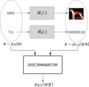
Figure 1: System model representation. $X$ is the input of a stochastic model $H(\cdot)$, while the output is $Y$. In the example represented by $H_{1}(\cdot)$, the input is the class element ”dog” and the output is an image of a dog. Differently, $H_{2}(\cdot)$ is a communication channel, therefore the input is a codeword, and the output is the binary representation of such a codeword after the noise addition.

In this section, we describe the perspective we propose to tackle classification tasks. Let $X$ and $Y$ be two random vectors described by the probability density functions $p_{X}(\mathbf{x})$ and $p_{Y}(\mathbf{y})$, respectively. Let $\mathcal{A}_{x}$ be the alphabet of $X$. Let $X$ and $Y$ be the input and output of a stochastic model (referred to as $H(\cdot)$), respectively, as shown in Fig. 1. In a classification context, $X$ represents the class type and $Y$ the observation of the class elements.
The MAP estimator (classifier) is formulated as:

$$\hat{\mathbf{x}}=\operatorname*{arg\,max}_{\mathbf{x}\in\Omega}p_{X|Y}(\mathbf{x}|\mathbf{y}),$$ (2)

where $p_{X|Y}(\mathbf{x}|\mathbf{y})$ is the posterior probability density. In this paper, we propose to adopt a discriminative formulation. Therefore, we express $p_{X|Y}(\mathbf{x}|\mathbf{y})$ as the ratio between $p_{XY}(\mathbf{x},\mathbf{y})$ and $p_{Y}(\mathbf{y})$ by using the Bayes theorem.
In a classification framework, the argmax operator can easily be computed when the posterior probability is known. Thus, the main goal is to estimate the posterior density. First, we study the more general problem of estimating the posterior density when $X$ is a continuous random vector. Then, we consider the specific case of $X$ being discrete. Finally, the latter estimation task leads us to the solution of the classification problem, by maximizing the posterior over the class elements (i.e., solving (2)).

III Posterior Probability Learning Through the Exploitation of $f$-Divergence

The first approach we propose is to estimate $p_{X|Y}(\mathbf{x}|\mathbf{y})$ by exploiting the variational representation of the $f$-divergence. Thus, we first recall the required definitions and then present a first class of estimators.

III-A $f$-Divergence

Given two probability distributions $P$ and $Q$ admitting, respectively, the absolutely continuous density functions $p$ and $q$ with respect to $d\mathbf{x}$ defined on the domain $\mathcal{X}$, the $f$-divergence (also known as Ali-Silvey distances) is defined as [24, 25]:

$$D_{f}(P||Q)=\int_{\mathcal{X}}q(\mathbf{x})f\left(\frac{p(\mathbf{x})}{q(\mathbf{x})}\right)d\mathbf{x},$$ (3)

where the generator function $f:\mathbb{R}_{+}\longrightarrow\mathbb{R}$ is a convex, lower-semicontinuous function such that $f(1)=0$. Every generator function has a Fenchel conjugate function $f^{*}$, that is defined as

$$f^{*}(t)=\sup_{u\in dom_{f}}\left\{ut-f(u)\right\},$$ (4)

where $dom_{f}$ is the domain of $f(\cdot)$, $f^{*}$ is convex and such that $f^{**}(u)=f(u)$.
Leveraging (4), the authors in [23] expressed a lower bound on any $f$-divergence, that is referred to as variational representation of the $f$-divergence:

$$D_{f}(P||Q) =\int_{\mathcal{X}}q(\mathbf{x})\sup_{t\in dom_{f^{*}}}\left\{\frac{p(\mathbf{x})}{q(\mathbf{x})}t-f^{*}(t)\right\}d\mathbf{x}$$

$$\geq\sup_{T\in\mathcal{T}}\left\{\int_{\mathcal{X}}p(\mathbf{x})T(\mathbf{x})d\mathbf{x}-\int_{\mathcal{X}}q(\mathbf{x})f^{*}(T(\mathbf{x}))d\mathbf{x}\right\}$$

$$=\sup_{T\in\mathcal{T}}\left\{\operatorname{\mathbb{E}}_{\mathbf{x}\sim p(\mathbf{x})}\left[T(\mathbf{x})\right]-\operatorname{\mathbb{E}}_{\mathbf{x}\sim q(\mathbf{x})}\left[f^{*}(T(\mathbf{x}))\right]\right\},$$ (5)

where $T(\mathbf{x})$ is parametrized by an artificial neural network, and the bound in (III-A) is tight when $T(\mathbf{x})$ is

$$T^{\diamond}(\mathbf{x})=f^{\prime}\left(\frac{p(\mathbf{x})}{q(\mathbf{x})}\right).$$ (6)

III-B Posterior Estimation Through the Variational Representation of the $f$-Divergence

Theorem 1 provides a class of objective functions that, when maximized, leads to the estimation of the posterior probability density.

Theorem 1.

Let $X$ and $Y$ be the random vectors with probability density functions $p_{X}(\mathbf{x})$ and $p_{Y}(\mathbf{y})$, respectively. Assume $\mathbf{y}=H(\mathbf{x})$, where $H(\cdot)$ is a stochastic function, then $p_{XY}(\mathbf{x},\mathbf{y})$ is the joint density. Define $\mathcal{T}_{x}$ to be the support of $X$ and $p_{U}(\mathbf{x})$ to be a uniform distribution with support $\mathcal{T}_{x}$. Let $f_{u}:\mathbb{R}_{+}\longrightarrow\mathbb{R}$ be a convex function such that $f_{u}(1)=0$, and $f_{u}^{*}$ be the Fenchel conjugate of $f_{u}$. Let $\mathcal{J}_{f}(T)$ be the objective function defined as

$$\mathcal{J}_{f}(T) =\operatorname{\mathbb{E}}_{(\mathbf{x},\mathbf{y})\sim p_{XY}(\mathbf{x},\mathbf{y})}\left[T(\mathbf{x},\mathbf{y})\right]$$

$$-\operatorname{\mathbb{E}}_{(\mathbf{x},\mathbf{y})\sim p_{U}(\mathbf{x})p_{Y}(\mathbf{y})}\left[f_{u}^{*}(T(\mathbf{x},\mathbf{y}))\right].$$ (7)

Then,

$$T^{\diamond}(\mathbf{x},\mathbf{y})=\operatorname*{arg\,max}_{T\in\mathcal{T}}\mathcal{J}_{f}(T)$$ (8)

leads to the estimation of the posterior density

$$\hat{p}_{X|Y}(\mathbf{x}|\mathbf{y})=\frac{p_{XY}(\mathbf{x},\mathbf{y})}{p_{Y}(\mathbf{y})}=\frac{(f_{u}^{*})^{\prime}(T^{\diamond}(\mathbf{x},\mathbf{y}))}{|\mathcal{T}_{x}|},$$ (9)

where $T^{\diamond}(\mathbf{x},\mathbf{y})$ is parametrized by an artificial neural network.

Proof.

From [23], $T^{\diamond}(\mathbf{x},\mathbf{y})$ as defined in (6) is achieved when maximizing (1). Lemma 1 in Appendix A-B states that $(f_{u}^{*})^{\prime}(T^{\diamond}(\mathbf{x},\mathbf{y}))=(f_{u}^{\prime})^{-1}(T^{\diamond}(\mathbf{x},\mathbf{y}))$, which is demonstrated by computing the first derivative of (4) after having substituted the optimal value of $u$ for which the supremum is achieved. Then, by inverting (6) and using Lemma 1, we obtain:

$$\frac{p_{XY}(\mathbf{x},\mathbf{y})}{p_{U}(\mathbf{x})p_{Y}(\mathbf{y})}=(f_{u}^{*})^{\prime}(T^{\diamond}(\mathbf{x},\mathbf{y})).$$ (10)

From [20], the usage of the uniform probability density function $p_{U}(\mathbf{x})$ is fundamental to define the objective function in (1). Its importance derives from the need of the discriminator to be fed with both $X$ and $Y$ realizations. Since $p_{U}(\mathbf{x})=\frac{1}{|\mathcal{T}_{x}|}$, as it is the uniform probability density function (pdf) over $\mathcal{T}_{x}$, the thesis follows. ∎

According to Theorem 1, there exists a class of objective functions to train a discriminator whose output is processed to obtain an estimate of the posterior probability. The choice of the $f$-divergence offers a degree of freedom (DOF) in the objective function design. To improve the training convergence of the objective functions formulated as variational representation of $f$-divergences, the literature exploits a change of variable $T(\mathbf{x},\mathbf{y})=r(D(\mathbf{x},\mathbf{y}))$ in (1) [22, 21]. With the same goal, we propose to introduce a second DOF in the development of the objective function. Accordingly, it is sufficient to substitute $D^{\diamond}(\mathbf{x},\mathbf{y})=r^{-1}(T^{\diamond}(\mathbf{x},\mathbf{y}))$ in (9) to attain the corresponding posterior probability estimator. The exploitation of the DOFs uniquely defines the objective function and numerically impacts the discriminator’s parameters convergence during the training phase.
This paper exploits the DOFs to develop five posterior probability estimators associated with the well-known $f$-divergences listed in Table I. The generator and Fenchel conjugate functions reported in Table I slightly differ from those used in other works [22, 21], since they include the Lebesgue measure $|\mathcal{T}_{x}|$. These functions, referred to as unsupervised, are attained as

$$f_{u}^{*}(t)=|\mathcal{T}_{x}|f^{*}(t),$$ (11)

where $f^{*}(t)$ is referred to as supervised version. Table I does not contain the constant terms that render $f_{u}(1)=0$, as their presence do not affect the objective functions. The procedure to obtain Table I is reported in Section A-A of the Appendix, along with Table II, reporting the supervised generator and Fenchel conjugate functions. Table III contains the objective functions corresponding to the five posterior probability estimators proposed, while all the mathematical derivations are reported in Appendix A-A. In addition, Table III comprises the change of variable $r(D^{\diamond}(\mathbf{x},\mathbf{y}))$ that is used to attain the corresponding objective function and the expression of $D^{\diamond}(\mathbf{x},\mathbf{y})$.

Lemma 2 proves the convergence property of any posterior probability estimator that is formulated as in Theorem 1.

Lemma 2.

Let the artificial neural network $D(\cdot)\in\mathcal{D}$. Let the set $\mathcal{D}$ be with enough capacity and training time (i.e., in the nonparametric limit). Let define

$$D^{\diamond}=\operatorname*{arg\,max}_{D\in\mathcal{D}}\mathcal{J}_{f}(D),$$ (12)

where $\mathcal{J}_{f}(D)$ is defined as in (1), with the change of variable $D=r^{-1}(T)$. Let consider the gradient ascent update rule

$$D^{(i+1)}=D^{(i)}+\mu\nabla\mathcal{J}_{f}(D^{(i)}),$$ (13)

where $D^{(i)}$ is the neural network at training iteration $i$, and $\mu>0$ the learning rate. Then, if $D^{\diamond}$ corresponds to the global optimum achieved by using the gradient ascent method, the posterior probability estimator in (9) converges to the real value of the posterior density.

Proof.

Similarly to Lemma 3 in [21], we define $\delta^{(i)}=r(D^{\diamond})-r(D^{(i)})$ as the difference between the optimum $T^{\diamond}$ and the one achieved at the $i^{th}$ iteration of the training procedure, when using a gradient ascent update method. Define $p^{(i)}$ and $p^{\diamond}$ as the posterior probability estimate at iteration $i$ and the optimum, respectively. Then,

$$p^{\diamond}-p^{(i)} =\frac{1}{|\mathcal{T}_{x}|}\Bigl{(}(f_{u}^{*})^{\prime}(r(D^{\diamond}))-(f_{u}^{*})^{\prime}(r(D^{(i)}))\Bigr{)}$$ (14)

$$=\frac{1}{|\mathcal{T}_{x}|}\Bigl{(}(f_{u}^{*})^{\prime}(r(D^{\diamond}))-(f_{u}^{*})^{\prime}(r(D^{\diamond})-\delta^{(i)})\Bigr{)}$$ (15)

$$\simeq\frac{1}{|\mathcal{T}_{x}|}\Bigl{(}\delta^{(i)}\Bigl{[}(f_{u}^{*})^{\prime\prime}(r(D^{\diamond})-\delta^{(i)})\Bigr{]}\Bigr{)},$$ (16)

where the last step develops from the first order Taylor expansion in $r(D^{\diamond})-\delta^{(i)}$. If the gradient ascent method converges towards the maximum, $\delta^{(i)}\longrightarrow 0$. Thus, when $i\longrightarrow\infty$, $|p^{\diamond}-p^{(i)}|\longrightarrow 0$. ∎

Lemma 2 does not only prove the convergence property of the posterior estimators in Theorem 1, it also offers a quantitative measure of the distance between the optimum posterior probability and the estimated one (see (16)).

Theorem 1 provides an effective method to solve classification problems by designing the objective function based on the choice of an $f$-divergence. This differs from other methods that leverage $f$-divergences and that need a dual optimization strategy [17, 18]. The proposed method relies on a single optimization problem. In fact, it generalizes the notorious cross-entropy minimization approach (see Appendix A-A). In the next section, we propose a novel bottom-up approach that guides the design of new objective functions for the posterior probability estimation problem.

TABLE I: $f$-divergences table. The corresponding $f$-divergences are: Kullback-Leibler, Reverse Kullback-Leibler, squared Hellinger distance, GAN, and Pearson $\chi^{2}$.

Name	$f_{u}(u)$	$f_{u}^{*}(t)$
KL	$u\log\left(\frac{u}{|\mathcal{T}_{x}|}\right)$	$|\mathcal{T}_{x}|\exp{(t-1)}$
RKL	$-|\mathcal{T}_{x}|\log(u)$	$-|\mathcal{T}_{x}|(1+\log(-t))$
HD	$(\sqrt{u}-\sqrt{|\mathcal{T}_{x}|})^{2}$	$|\mathcal{T}_{x}|\frac{t}{1-t}$
GAN	$u\log(u)-(u+|\mathcal{T}_{x}|)\log(u+|\mathcal{T}_{x}|)$	$-|\mathcal{T}_{x}|\log(1-\exp{(t)})$
P	$\frac{1}{|\mathcal{T}_{x}|}(u-|\mathcal{T}_{x}|)^{2}$	$|\mathcal{T}_{x}|\left(\frac{1}{4}t^{2}+t\right)$

TABLE III: Objective functions table. The corresponding $f$-divergences are: Kullback-Leibler, Reverse Kullback-Leibler, squared Hellinger distance, GAN, and Pearson $\chi^{2}$.

Name	Objective function	$T^{\diamond}(\mathbf{x},\mathbf{y})$	$D^{\diamond}(\mathbf{x},\mathbf{y})$
$\mathcal{J}_{KL}(D)$	$\operatorname{\mathbb{E}}_{(\mathbf{x},\mathbf{y})\sim p_{XY}(\mathbf{x},\mathbf{y})}\Bigl{[}\log(D(\mathbf{x},\mathbf{y}))\Bigr{]}-\operatorname{\mathbb{E}}_{(\mathbf{x},\mathbf{y})\sim p_{U}(\mathbf{x})p_{Y}(\mathbf{y})}\Bigl{[}|\mathcal{T}_{x}|D(\mathbf{x},\mathbf{y})\Bigr{]}$	$\log(D^{\diamond}(\mathbf{x},\mathbf{y}))+1$	$\frac{p_{XY}(\mathbf{x},\mathbf{y})}{p_{Y}(\mathbf{y})}$
$\mathcal{J}_{RKL}(D)$	$\operatorname{\mathbb{E}}_{(\mathbf{x},\mathbf{y})\sim p_{XY}(\mathbf{x},\mathbf{y})}\Bigl{[}-D(\mathbf{x},\mathbf{y})\Bigr{]}-\operatorname{\mathbb{E}}_{(\mathbf{x},\mathbf{y})\sim p_{U}(\mathbf{x})p_{Y}(\mathbf{y})}\Bigl{[}|\mathcal{T}_{x}|\log(D(\mathbf{x},\mathbf{y}))\Bigr{]}$	$-D^{\diamond}(\mathbf{x},\mathbf{y})$	$\frac{p_{Y}(\mathbf{y})}{p_{XY}(\mathbf{x},\mathbf{y})}$
$\mathcal{J}_{HD}(D)$	$\operatorname{\mathbb{E}}_{(\mathbf{x},\mathbf{y})\sim p_{XY}(\mathbf{x},\mathbf{y})}\Bigl{[}-\sqrt{D(\mathbf{x},\mathbf{y})}\Bigr{]}-\operatorname{\mathbb{E}}_{(\mathbf{x},\mathbf{y})\sim p_{U}(\mathbf{x})p_{Y}(\mathbf{y})}\Bigl{[}|\mathcal{T}_{x}|\frac{1}{\sqrt{D(\mathbf{x},\mathbf{y})}}\Bigr{]}$	$1-\sqrt{D^{\diamond}}$	$\frac{p_{Y}(\mathbf{y})}{p_{XY}(\mathbf{x},\mathbf{y})}$
$\mathcal{J}_{GAN}(D)$	$\operatorname{\mathbb{E}}_{(\mathbf{x},\mathbf{y})\sim p_{XY}(\mathbf{x},\mathbf{y})}\Bigl{[}\log(1-D(\mathbf{x},\mathbf{y}))\Bigr{]}+\operatorname{\mathbb{E}}_{(\mathbf{x},\mathbf{y})\sim p_{U}(\mathbf{x})p_{Y}(\mathbf{y})}\Bigl{[}|\mathcal{T}_{x}|\log(D(\mathbf{x},\mathbf{y}))\Bigr{]}$	$\log(1-D^{\diamond}(\mathbf{x},\mathbf{y}))$	$\frac{p_{Y}(\mathbf{y})}{p_{XY}(\mathbf{x},\mathbf{y})+p_{Y}(\mathbf{y})}$
$\mathcal{J}_{P}(D)$	$\operatorname{\mathbb{E}}_{(\mathbf{x},\mathbf{y})\sim p_{XY}(\mathbf{x},\mathbf{y})}\Bigl{[}2(D(\mathbf{x},\mathbf{y})-1)\Bigr{]}-\operatorname{\mathbb{E}}_{(\mathbf{x},\mathbf{y})\sim p_{U}(\mathbf{x})p_{Y}(\mathbf{y})}\Bigl{[}|\mathcal{T}_{x}|D^{2}(\mathbf{x},\mathbf{y})\Bigr{]}$	$2(D^{\diamond}(\mathbf{x},\mathbf{y})-1)$	$\frac{p_{XY}(\mathbf{x},\mathbf{y})}{p_{Y}(\mathbf{y})}$

IV Bottom-Up Posterior Probability Learning

In this section, we follow a different approach with respect to the one in the previous section. It allows us to propose a bottom-up methodology for developing objective functions that, when maximized, lead to the estimate of the posterior probability. The bottom-up approach reverses the top-down procedure typical of $f$-divergence formulations [26, 21]. The main advantage of this new method is that it guides the design of the objective function by starting with the imposition of the optimal convergence condition of the discriminator’s output $D^{\diamond}(\mathbf{x},\mathbf{y})$. Theorem 2 presents the class of objective functions that, when maximized, leads to the bottom-up posterior estimator.

Theorem 2.

Let $X$ and $Y$ be the random vectors with probability density functions $p_{X}(\mathbf{x})$ and $p_{Y}(\mathbf{y})$, respectively. Assume $\mathbf{y}=H(\mathbf{x})$, where $H(\cdot)$ is a stochastic function, then $p_{XY}(\mathbf{x},\mathbf{y})$ is the joint density. Let $\mathcal{T}_{x}$ and $\mathcal{T}_{y}$ be the support of $p_{X}(\mathbf{x})$ and $p_{Y}(\mathbf{y})$, respectively. Let the discriminator $D(\mathbf{x},\mathbf{y})$ be a scalar function of $\mathbf{x}$ and $\mathbf{y}$. Let $k(\cdot)$ be any deterministic and invertible function. Then, the posterior density is estimated as

$$\hat{p}_{X|Y}(\mathbf{x}|\mathbf{y})=k^{-1}(D^{\diamond}(\mathbf{x},\mathbf{y})),$$ (17)

where $D^{\diamond}(\mathbf{x},\mathbf{y})$ is the optimal discriminator obtained by maximizing

$$\mathcal{J}(D)=\int_{\mathcal{T}_{x}}\int_{\mathcal{T}_{y}}\tilde{\mathcal{J}}(D)d\mathbf{x}d\mathbf{y},$$ (18)

for all concave functions $\tilde{\mathcal{J}}(D)$ such that their first derivative is

$$\frac{\partial\tilde{\mathcal{J}}(D)}{\partial D} =\Bigl{(}D(\mathbf{x},\mathbf{y})-k(p_{X|Y}(\mathbf{x}|\mathbf{y}))\Bigr{)}g_{1}(D,k)$$

$$\triangleq g(D,k)$$ (19)

with $g_{1}(D,k)\neq 0$ deterministic, and

$$g_{1}(D,k)\leq(k(p_{X|Y}(\mathbf{x}|\mathbf{y}))-D(\mathbf{x},\mathbf{y}))\left(\frac{\partial g_{1}(D,k)}{\partial D}\right).$$ (20)

Proof.

A necessary condition to maximize $\mathcal{J}(D)$ requires to set the first derivative of the integrand $\tilde{\mathcal{J}}(D)$ w.r.t. $D$ equal to zero. Since $g_{1}(D,k)\neq 0$, from (2) easily follows

$$D^{\diamond}(\mathbf{x},\mathbf{y})=k(p_{X|Y}(\mathbf{x}|\mathbf{y}))=k\left(\frac{p_{XY}(\mathbf{x},\mathbf{y})}{p_{Y}(\mathbf{y})}\right).$$ (21)

The condition in (20) is obtained by imposing the first derivative of $g(D,k)$ (in (2)) with respect to $D$ to be nonpositive. Therefore, the stationary point in (20) corresponds to a maximum because the second derivative of the objective function w.r.t. $D$ is a nonpositive function thanks to (20). ∎

The proposed estimator leverages a discriminative formulation to estimate the density ratio corresponding to the posterior probability. In addition, Theorem 2 comprises two DOFs in the objective function design. The former is the choice of $k(\cdot)$, since we propose that the discriminator estimates an invertible transformation of the posterior density. We noticed that the classifier performs better when $k(\cdot)$ is chosen to resemble particular activation functions. The motivation is that the activation function of the last layer has to be chosen coherently with the objective function. The second DOF, represented by $g_{1}(\cdot)$, is a rearrangement term that modifies the result of the integration of $g(\cdot)$ with respect to $D$. The exploitation of such a DOF allows to attain different objective functions even when imposing the same optimal discriminator’s output.

Corollary 2.1 exploits the DOF in the choice of $k(\cdot)$ and $g_{1}(\cdot)$ to design and obtain the objective functions in Table III, which were previously derived acording to the method leading to Theorem 1.

Corollary 2.1.

Let $\mathcal{J}(D)$ be defined as in Theorem 2. Let

$$k(p_{X|Y}(\mathbf{x}|\mathbf{y}))=k\left(\frac{p_{XY}(\mathbf{x},\mathbf{y})}{|\mathcal{T}_{x}|p_{U}(\mathbf{x})p_{Y}(\mathbf{y})}\right)=\frac{p_{0}}{p_{1}}.$$ (22)

Define

$$g_{1}(D,k;\alpha,\beta)\triangleq-\frac{p_{1}}{D^{\alpha}}\left(\frac{1}{1-D}\right)^{\beta},$$ (23)

where $\alpha,\beta\in\mathbb{Q}$. Then, for each divergence $f$, the objective functions in Table III are obtained from Theorem 2 by using $k(\cdot)$ and the parameters $\alpha,\beta$ of $g_{1}(\cdot)$ as defined in the set $\mathcal{F}_{k,g_{1}}\triangleq\{(k(x),(\alpha,\beta))_{f}\}$:

$$\mathcal{F}_{k,g_{1}}= \Biggl{\{}\Biggl{(}x,\left(1,0\right)\Biggr{)}_{KL},\Biggl{(}-\frac{1}{x},\left(1,0\right)\Biggr{)}_{RKL},$$

$$\Biggl{(}\frac{1}{x},\left(\frac{3}{2},0\right)\Biggr{)}_{HD},\Biggl{(}\frac{1}{1+x},\left(1,1\right)\Biggr{)}_{GAN},$$ (24)

$$\Biggl{(}x,(0,0)\Biggr{)}_{P}\Biggr{\}}$$ (25)

Proof.

The proof directly follows from Theorem 2 and is reported in Appendix A-B. ∎

Theorems 1 and 2 have different advantages. The advantage of Theorem 1 is its simple applicability, but it needs to start with a choice of the generator function $f$ to be used. The benefit of using Theorem 2 is that it guides the objective function design without relying on existing $f$-divergences.
An interesting result highlighted by Corollary 2.1 is that all the objective functions corresponding to the well-known $f$-divergences in Table I use the same class of functions $g_{1}(\cdot)$ expressed in (23). This property, which the bottom-up estimator highlights, showed us that the $\mathcal{J}_{GAN}(D)$ is the only one using $\beta=1$. Thanks to the observation of this peculiarity and driven by curiosity, we develop a new objective function starting from the same $k(\cdot)$ and $g_{1}(\cdot)$ but imposing $\beta=0$.

V Shifted Log Objective Function and $f$-Divergence

In this section, we present a new objective function for classification problems, that we design by using Theorem 2. Then, we prove that such an objective function corresponds to the variational representation of a novel $f$-divergence, called shifted log (SL). We will demonstrate in Section VII that such a new objective function achieves the best performance in almost all the classification scenarios discussed.

Theorem 3.

Let $X$ and $Y$ be two random vectors with pdfs $p_{X}(\mathbf{x})$ and $p_{Y}(\mathbf{y})$, respectively. Assume $Y=H(X)$, with $H(\cdot)$ stochastic function, then let $p_{XY}(\mathbf{x},\mathbf{y})$ be the joint density. Let $\mathcal{T}_{x}$ be the support of $X$. Let $p_{U}(\mathbf{x})$ be a uniform pdf having the same support $\mathcal{T}_{x}$. The maximization of the objective function

$$\mathcal{J}_{SL}(D) =-\operatorname{\mathbb{E}}_{(\mathbf{x},\mathbf{y})\sim p_{XY}(\mathbf{x},\mathbf{y})}\Bigl{[}D(\mathbf{x},\mathbf{y})\Bigr{]}$$

$$+\operatorname{\mathbb{E}}_{(\mathbf{x},\mathbf{y})\sim p_{U}(\mathbf{x})p_{Y}(\mathbf{y})}\Bigl{[}|\mathcal{T}_{x}|\Bigl{(}\log(D(\mathbf{x},\mathbf{y}))-D(\mathbf{x},\mathbf{y})\Bigr{)}\Bigr{]},$$ (26)

leads to the optimal discriminator output

$$D^{\diamond}(\mathbf{x},\mathbf{y})=\operatorname*{arg\,max}_{D}\mathcal{J}_{SL}(D)=\frac{1}{1+p_{X|Y}(\mathbf{x},\mathbf{y})},$$ (27)

and the posterior density estimate is computed as

$$\hat{p}_{X|Y}(\mathbf{x}|\mathbf{y})=\frac{1-D^{\diamond}(\mathbf{x},\mathbf{y})}{D^{\diamond}(\mathbf{x},\mathbf{y})}.$$ (28)

Proof.

Following Theorem 2, the proof starts by inverting (17). Specifically, we set $k(x)=\frac{1}{1+x}$ and from (27), by expressing the posterior density as the density ratio $p_{XY}/p_{Y}$, we achieve

$$D^{\diamond}(\mathbf{x},\mathbf{y})-\frac{|\mathcal{T}_{x}|p_{U}(\mathbf{x})p_{Y}(\mathbf{y})}{|\mathcal{T}_{x}|p_{U}(\mathbf{x})p_{Y}(\mathbf{y})+p_{XY}(\mathbf{x},\mathbf{y})}=0,$$ (29)

where $p_{U}(\mathbf{x})=1/|\mathcal{T}_{x}|$. Then, (23) with $\alpha=1$ and $\beta=0$ becomes

$$g_{1}(D,k;1,0) =-\frac{|\mathcal{T}_{x}|p_{U}(\mathbf{x})p_{Y}(\mathbf{y})+p_{XY}(\mathbf{x},\mathbf{y})}{D(\mathbf{x},\mathbf{y})}.$$ (30)

Then, (30) is substituted in (2):

$$g(D,k)=\frac{\partial}{\partial D}\mathcal{\tilde{J}}(D)= -\Bigl{(}|\mathcal{T}_{x}|p_{U}(\mathbf{x})p_{Y}(\mathbf{y})+p_{XY}(\mathbf{x},\mathbf{y})\Bigr{)}$$

$$+\frac{|\mathcal{T}_{x}|p_{U}(\mathbf{x})p_{Y}(\mathbf{y})}{D(\mathbf{x},\mathbf{y})}.$$ (31)

The computation of the integral of (V) with respect to the discriminator’s output $D$ leads to

$$\tilde{\mathcal{J}}(D) =-p_{XY}(\mathbf{x},\mathbf{y})D(\mathbf{x},\mathbf{y})$$

$$+|\mathcal{T}_{x}|p_{U}(\mathbf{x})p_{Y}(\mathbf{y})\Bigl{(}\log(D(\mathbf{x},\mathbf{y}))-D(\mathbf{x},\mathbf{y})\Bigr{)},$$ (32)

which proves the statement of the theorem, since (20) is verified because

$$\frac{\partial g(D,k)}{\partial D}=-\frac{p_{Y}(\mathbf{y})}{D^{2}(\mathbf{x},\mathbf{y})}\leq 0.$$ (33)

Given the optimum discriminator $D^{\diamond}$, the posterior density estimator in (28) is achieved by inverting (27). ∎

Corollary 3.1.

Define the generator function

$$f_{u,SL}(u)=-|\mathcal{T}_{x}|\log(u+|\mathcal{T}_{x}|)+K,$$ (34)

where $K=|\mathcal{T}_{x}|\log(1+|\mathcal{T}_{x}|)$ is constant. Then, $\mathcal{J}_{SL}(D)$ in (3) is the variational representation of $D_{f_{u,SL}}(p_{XY}||p_{Y})$.

Proof.

By comparing (3) to (1), it is immediate to notice the change of variable $D(\mathbf{x},\mathbf{y})=-T(\mathbf{x},\mathbf{y})$. Then, the expression of the Fenchel conjugate is attained as $f_{u,SL}^{*}(t)=-|\mathcal{T}_{x}|(\log(-t)+t)$ from the expectation over $p_{U}(\mathbf{x})p_{Y}(\mathbf{y})$. The generating function $f_{u,SL}(u)=-|\mathcal{T}_{x}|\log(u+|\mathcal{T}_{x}|)$ is computed by using the definition of Fenchel conjugate. We add a constant $K=|\mathcal{T}_{x}|\log(1+|\mathcal{T}_{x}|)$ to the generator function to achieve the condition $f(1)=0$, which has no impact on the maximization of the objective function in (3). Lastly, the second derivatives of $f_{u,SL}(u)$ and $f_{u,SL}^{*}(t)$ are nonpositive functions, proving that the generator function and its Fenchel conjugate are convex. ∎

In the next paragraphs, we discuss some properties of the objective function and $f$-divergence proposed in Theorem 3.

V-A Remarks on the New Objective Function and $f$-Divergence

Since the proposed objective function in (3) is the variational representation of an $f$-divergence, Lemma 2 ensures the convergence property of its estimate to the true posterior probability in the nonparametric limit.

The supervised version of the SL divergence is

$$f_{SL}(u)=-\log(u+1)+\log(2),$$ (35)

which is obtained by substituting $|\mathcal{T}_{x}|=1$ (see Appendix A-A). Although $f_{SL}$ is obtained in the context of posterior estimation problems, the proposed $f$-divergence can be applied to a broader variety of tasks. Since $D_{SL}$ is upper-bounded (see Corollary 3.2), it is a suitable generator function when the optimization problem requires to maximize the $f$-divergence. For instance, when the objective function is formulated as a max-max game, as in [27], where the mutual information is maximized to achieve the channel capacity in a data communication system. Corollary 3.2 provides the upper and lower bound of the SL divergence.

Corollary 3.2.

Let $P$ and $Q$ be two probability distributions. Let $D_{SL}(P||Q)$ be the $f$-divergence with generator function $f_{SL}(u)$ as in (35). Then,

$$0\leq D_{SL}(P||Q)\leq\log(2).$$ (36)

Proof.

Let $f:\mathbb{R}_{+}\longrightarrow\mathbb{R}$ be a convex function with $f(1)=0$, and $f^{\circ}:\mathbb{R}_{+}\longrightarrow\mathbb{R}$ defined as

$$f^{\circ}(u)\triangleq uf\left(\frac{1}{u}\right),$$ (37)

then $f^{\circ}$ is also convex and such that $f^{\circ}(1)=0$. Then, the Range of Values Theorem [28] sets upper and lower bounds on the value of the $f$-divergence between two distributions $P$ and $Q$, depending on $f(u)$ and $f^{\circ}(u)$:

$$f(1)\leq D_{f}(P||Q)\leq f(0)+f^{\circ}(0)\>\>\>\>\>\forall Q,P.$$ (38)

From which the thesis follows. ∎

V-B Comparison Between SL and GAN Divergences

The GAN divergence is known to be highly-performing in a wide variety of tasks [21, 26]. Moreover, the objective functions corresponding to SL and GAN divergences can be obtained from Theorem 2 by choosing the same $k(\cdot)$, but different $g_{1}(\cdot)$. Corollary 3.3 compares the shape of the two objective functions in the neighborhood of the global optimum.

Corollary 3.3.

Let $\mathcal{J}_{SL}(D)$ be defined as in (3). Let $\mathcal{J}_{GAN}(D)$ be defined as in Table III. Let $D^{\diamond}_{N}$ be the discriminator output in a neighborhood of $D^{\diamond}$ where $\mathcal{J}_{SL}(D^{\diamond}_{N})$ and $\mathcal{J}_{GAN}(D^{\diamond}_{N})$ are concave. Then,

$$\Bigg{|}\frac{\partial\mathcal{J}_{GAN}(D^{\diamond}_{N})}{\partial D}\Bigg{|}\geq\Bigg{|}\frac{\partial\mathcal{J}_{SL}(D^{\diamond}_{N})}{\partial D}\Bigg{|}.$$ (39)

Proof.

To prove (39), we just need to prove

$$\Bigg{|}\frac{\partial\tilde{\mathcal{J}}_{GAN}(D^{\diamond}_{N})}{\partial D}\Bigg{|}\geq\Bigg{|}\frac{\partial\tilde{\mathcal{J}}_{SL}(D^{\diamond}_{N})}{\partial D}\Bigg{|},$$ (40)

(where $\tilde{\mathcal{J}}$ is the integrand function in (18)) since the inequality between the integrands holds when the integrals are computed over the same interval.
Lemma 2 guarantees the convergence to the optimal discriminator. Therefore, let $D^{\diamond}_{N}=\frac{p_{Y}(\mathbf{y})}{p_{XY}(\mathbf{x},\mathbf{y})+p_{Y}(\mathbf{y})}+\delta$, with $\delta$ arbitrarily small, so that $D^{\diamond}_{N}$ belongs to the neighborhood of $D^{\diamond}$. Then,

$$\frac{\partial}{\partial D}\tilde{\mathcal{J}}_{SL}(D)\Bigg{|}_{D^{\diamond}_{N}} =-(p_{XY}(\mathbf{x},\mathbf{y})+p_{Y}(\mathbf{y}))+\frac{p_{Y}(\mathbf{y})}{D^{\diamond}_{N}(\mathbf{x},\mathbf{y})}$$ (41)

$$\frac{\partial}{\partial D}\tilde{\mathcal{J}}_{GAN}(D)\Bigg{|}_{D^{\diamond}_{N}} =-\frac{p_{XY}(\mathbf{x},\mathbf{y})}{1-D^{\diamond}_{N}(\mathbf{x},\mathbf{y})}+\frac{p_{Y}(\mathbf{y})}{D^{\diamond}_{N}(\mathbf{x},\mathbf{y})}$$

$$=-\frac{p_{XY}(\mathbf{x},\mathbf{y})(p_{XY}(\mathbf{x},\mathbf{y})+p_{Y}(\mathbf{y}))}{p_{XY}(\mathbf{x},\mathbf{y})(1-\delta)-\delta p_{Y}(\mathbf{y})}$$

$$+\frac{p_{Y}(\mathbf{y})}{D^{\diamond}_{N}(\mathbf{x},\mathbf{y})}$$ (42)

By substituting $\gamma=\frac{1}{1-\delta}$, (42) becomes

$$\frac{\partial}{\partial D}\tilde{\mathcal{J}}_{GAN}(D)\Bigg{|}_{D^{\diamond}_{N}} \approx-\gamma(p_{XY}(\mathbf{x},\mathbf{y})+p_{Y}(\mathbf{y}))+\frac{p_{Y}(\mathbf{y})}{D^{\diamond}_{N}(\mathbf{x},\mathbf{y})},$$ (43)

where $0<\gamma<1$ if $\delta<0$, and $\gamma>1$ if $\delta>0$. Thus, the comparison between (41) and (43) leads to the inequalities

$$\frac{\partial}{\partial D}\tilde{\mathcal{J}}_{SL}(D)\Bigg{|}_{D^{\diamond}_{N}} <\frac{\partial}{\partial D}\tilde{\mathcal{J}}_{GAN}(D)\Bigg{|}_{D^{\diamond}_{N}}\quad if\delta<0$$ (44)

$$\frac{\partial}{\partial D}\tilde{\mathcal{J}}_{SL}(D)\Bigg{|}_{D^{\diamond}_{N}} >\frac{\partial}{\partial D}\tilde{\mathcal{J}}_{GAN}(D)\Bigg{|}_{D^{\diamond}_{N}}\quad if\delta>0.$$ (45)

Since $D^{\diamond}$ corresponds to a maximum, i.e., the sign of the left derivative is positive, and the sign of the right derivative is negative, the statement of the corollary is proved.

∎

Although the shape of the loss landscape depends on many factors (e.g., the batch size [29, 30]), sharper maxima attain larger test error [31]. The steepness of the concavity of the objective function in the neighborhood of the global optimum provides insights on the basin of attraction of the maximum point. Intuitively, a flatter landscape corresponds to a larger basin of attraction of the global optimum, rendering training with the SL divergence better than with the GAN divergence. The results in Section VII validate the effectiveness of Corollary 3.3.

VI Discriminator Architecture

(a) Unsupervised architecture

(b) Supervised architecture

Figure 2: Diagrams of unsupervised and supervised architectures. The thick black line represents the discriminator box in Figure 1. The trapezoidal shape represents the neural network architecture.

The results obtained so far allow the estimation of the posterior probability for the case of $p_{X}(\mathbf{x})$ continuous pdf. In this section, we discuss the appropriate modifications to the architecture of the discriminator to suit our estimators to the classification case, where the number of classes is finite. The architecture type used differs depending on the alphabet of $X$, called $\mathcal{A}_{x}$. When $X$ is continuous (i.e., $|\mathcal{A}_{x}|\geq|\mathbb{R}|$), we use a structure referred to as unsupervised architecture. Differently, when $X$ is discrete (i.e., $|\mathcal{A}_{x}|\leq|\mathbb{N}|$), we use a structure referred to as supervised architecture.
The two architecture types are trained and tested by using the same approach. The training part consists in the alternation of two phases. In the former phase, the network is fed with $N$ realizations of the joint distribution $p_{XY}(\mathbf{x},\mathbf{y})$ to compute the first term of the objective function. In the latter phase, the same network is fed with $N$ samples drawn from $p_{U}(\mathbf{x})p_{Y}(\mathbf{y})$ to compute the second term of the objective function. The total loss is obtained as the summation of the two terms, then backpropagation [32] is applied.
During the test part, the network is fed with the samples drawn from the joint distribution, and the posterior probability density estimate is obtained as in (9) or (17).

VI-A Unsupervised Architecture

In this setting, the samples $\mathbf{x}$ and $\mathbf{y}$ drawn from the empirical probability distributions $p_{XY}(\mathbf{x},\mathbf{y})$ and $p_{U}(\mathbf{x})p_{Y}(\mathbf{y})$ are concatenated and fed into the discriminator. This architectural characterization reflects the notation, i.e., $D(\mathbf{x},\mathbf{y})$. The discriminator output is a scalar, since it is the posterior density function estimate corresponding to the couple $(\mathbf{x},\mathbf{y})$ given as input. The discriminator architecture is represented in Figure 2(a), where the concatenation between the $\mathbf{x}$ and $\mathbf{y}$ realizations is identified by a dashed rectangle.

VI-B Supervised Architecture

The supervised discriminator architecture is reported in Figure 2(b). The supervised architecture introduces in the problem’s formulation the constraint that $\mathcal{A}_{x}$ is a set containing a finite number of elements $\mathcal{A}_{x}=\left\{\mathbf{x}_{1},\dots,\mathbf{x}_{m}\right\}$. This constraint is embedded in the neural network architecture (highlighted by a dashed arrow in Figure 2(b)), so that the output layer contains one neuron for each sample in $\mathcal{A}_{x}$. With this modification, the i-th output neuron returns $p_{X|Y}(\mathbf{x}_{i}|\mathbf{y})$. Accordingly, the input layer is fed with only $\mathbf{y}$ realizations. Notation wise, the imposed constraint implies that the output of the discriminator must be expressed only as function of the $\mathbf{y}$ realizations. Therefore, the discriminator’s output is referred to as $\textbf{D}(\mathbf{y})$.

The objective functions provided in the general case must be slightly modified as a result of the architectural modification. Theorem 4 shows the formulation of the objective functions in (1) when using a supervised architecture. First, we define the notation useful for the theorem statement:

$$\textbf{D}(\mathbf{y})=\begin{pmatrix}D(x_{1},\mathbf{y})\\ D(x_{2},\mathbf{y})\\ \vdots\\ D(x_{m},\mathbf{y})\end{pmatrix}\textbf{1}_{m}=\begin{pmatrix}1\\ 1\\ \vdots\\ 1\end{pmatrix}\textbf{1}_{m}(\mathbf{x}_{i})=\begin{pmatrix}0\\ \vdots\\ 0\\ \underbrace{1}_{i^{th}\>\>pos.}\\ 0\\ \vdots\\ 0\end{pmatrix}.$$ (46)

Theorem 4.

Let $p_{X}(\mathbf{x})$ and $p_{Y}(\mathbf{y})$ be pdfs describing the input and output of a stochastic function $H(\cdot)$, respectively. Let $p_{X}(\mathbf{x})\triangleq\sum_{i=1}^{m}P_{X}(\mathbf{x}_{i})\delta(\mathbf{x}-\mathbf{x}_{i})$, where $P_{X}(\cdot)$ is the probability mass function of $X$. Let $\mathcal{T}_{x}$ be the support of $p_{X}(\mathbf{x})$ and $|\mathcal{T}_{x}|$ its Lebesgue measure. Let $p_{U}(\mathbf{x})$ be the uniform discrete probability density function over $\mathcal{T}_{x}$. Let the discriminator be characterized by a supervised architecture. Then, the objective function in (1) becomes

$$\mathcal{J}(D) =\operatorname{\mathbb{E}}_{\mathbf{x}\sim p_{X}(\mathbf{x})}\Biggl{[}\operatorname{\mathbb{E}}_{\mathbf{y}\sim p_{Y|X}(\mathbf{y}|\mathbf{x})}\Bigl{[}r(\textbf{D}(\mathbf{y}))^{T}\textbf{1}_{m}(\mathbf{x})\Bigr{]}\Biggr{]}$$

$$-\operatorname{\mathbb{E}}_{\mathbf{y}\sim p_{Y}(\mathbf{y})}\Bigl{[}\left(f^{*}\left(r(\textbf{D}(\mathbf{y}))\right)\right)^{T}\textbf{1}_{m}\Bigr{]},$$ (47)

where $T(\mathbf{y})=r(D(\mathbf{y}))$.

Proof.

Let the alphabet of $X$ be $\mathcal{A}_{x}=\left\{\mathbf{x}_{1},\dots,\mathbf{x}_{m}\right\}$. The objective function in (1) can be expressed as

$$\mathcal{J}(D) =\int_{\mathcal{T}_{y}}\int_{\mathcal{T}_{x}}p_{X}(\mathbf{x})p_{Y|X}(\mathbf{y}|\mathbf{x})r(D(\mathbf{x},\mathbf{y}))$$

$$-p_{U}(\mathbf{x})p_{Y}(\mathbf{y})f_{u}^{*}\left(r(D(\mathbf{x},\mathbf{y}))\right)d\mathbf{x}d\mathbf{y}.$$ (48)

Then, let $p_{U}(\mathbf{x})\triangleq\sum_{i=1}^{m}P_{U}(\mathbf{x}_{i})\delta(\mathbf{x}-\mathbf{x}_{i})$, with $P_{U}(\mathbf{x}_{i})=\frac{1}{|\mathcal{T}_{x}|}$.

$$\mathcal{J}(D) =\int_{\mathcal{T}_{y}}\int_{\mathcal{T}_{x}}\sum_{i=1}^{m}P_{X}(\mathbf{x}_{i})\delta(\mathbf{x}-\mathbf{x}_{i})p_{Y|X}(\mathbf{y}|\mathbf{x})r(D(\mathbf{x},\mathbf{y}))$$

$$-\sum_{i=1}^{m}\delta(\mathbf{x}-\mathbf{x}_{i})p_{Y}(\mathbf{y})f^{*}\left(r(D(\mathbf{x},\mathbf{y}))\right)d\mathbf{x}d\mathbf{y},$$ (49)

where $f_{u}^{*}\left(r(D(\mathbf{x},\mathbf{y}))\right)=|\mathcal{T}_{x}|f^{*}\left(r(D(\mathbf{x},\mathbf{y}))\right)$. Then, by using the indicator property of the delta function, the objective function becomes

$$\mathcal{J}(D) =\int_{\mathcal{T}_{y}}\sum_{i=1}^{m}P_{X}(\mathbf{x}_{i})p_{Y|X}(\mathbf{y}|\mathbf{x}_{i})r(D(\mathbf{x}_{i},\mathbf{y}))d\mathbf{y}$$

$$-\int_{\mathcal{T}_{y}}p_{Y}(\mathbf{y})\sum_{i=1}^{m}f^{*}\left(r(D(\mathbf{x}_{i},\mathbf{y}))\right)d\mathbf{y},$$ (50)

that is equivalent to (4). ∎

The supervised versions of the objective functions proposed in the paper are listed in Section A-A of the Appendix.

VII Results

In this section, we report several numerical results to assess the validity of the methods proposed to estimate the posterior probability and enable the classification task. The considered scenarios are:

• classification for image data sets;

• signal decoding in telecommunications engineering cast into a classification task;

• posterior probability estimation when $p_{X}(\mathbf{x})$ is continuous.

The results demonstrate that different $f$-divergences attain different performance, consistently with Lemma 2. We show that the KL divergence is not necessarily the best divergence choice for classification tasks, and more in general for probability estimation problems. We demonstrate that the SL divergence achieves the best performance in almost all the tested contexts.
The first two scenarios are classification problems, therefore we use the supervised formulation of the discriminator architecture. The third scenario comprises two toy cases, where we show that the unsupervised formulation of the proposed estimators works also for continuous random vectors $X$. Thus, we prove that the general formulation before Section VI is theoretically and experimentally important.
Before discussing the numerical results, we briefly describe the details of the code implementation.

VII-A Implementation Details

For fair comparison, we use the same architecture and hyper-parameters for each estimator.

Supervised Architecture: We use convolutional neural networks for the first scenario and fully connected feedforward neural networks for the second scenario. For each image data set, we use a discriminator comprising a set of convolutional layers followed by a feedforward fully connected part. The discriminator parameters slightly vary depending on the data set tested. The LeakyReLU activation function is used in all the layers except the last one, where the activation function is chosen based on the objective function optimized for the training phase. The network parameters are updated by using the Adam optimizer [33]. In some cases, the Dropout technique [34] helps the convergence of the training process. When specified in the results, the ResNet [35] model is utilized.
The architecture used for the decoding scenario comprises two hidden layers with $100$ neurons each. The LeakyReLU activation function is utilized in all the layers except the last one, where it is chosen based on the objective function optimized. Dropout is used during training.

Unsupervised Architecture: The discriminator architecture utilized for the unsupervised tasks comprises two hidden layers with $100$ neurons each, with the LeakyReLU and Sigmoid activation functions used. The activation function of the output layer depends on the objective function used during training. The network weights and biases are updated by using Adam optimizer. Dropout is used during training.

VII-B Image Datasets Classification

The first scenario tackled is the classification of image data sets. The objective functions effectiveness is tested for the MNIST [36], FashionMNIST [37], and CIFAR10 [38] data sets. We compare the classification accuracy of the supervised versions of the objective functions in Table III and in (3). For each data set, we run the tests with multiple random seeds to show the robustness of the proposed estimators and to obtain fully reproducible results. We computed the mean accuracy and root mean squared error (RMSE) for each data set and $f$-divergence using the shallow discriminator architecture previously described. The results are reported in Table IV. The accuracies displayed in Table IV confirm that each generator function has a different impact on the neural network training, as also shown in [21, 26]. The difference in the performance attained is visible. The SL divergence attains the highest classification accuracy in almost all the datasets tested, showing its effectiveness compared to the other divergences and, in particular, to the KL that corresponds to the state-of-the-art approach (see the KL paragraph in Appendix A-A). The CIFAR10 data set is the most challenging. Thus, more complex architectures must be used, as we verified by developing additional tests reported in Table V. Table V reports the accuracy achieved by each posterior probability estimator on the CIFAR10 data set when using ResNet18 and ResNet50 architectures. The increase in complexity of the architecture enlarges the difference in the achieved accuracy. Similarly to the shallow discriminator architecture case, the SL divergence achieves the best performance.

TABLE IV: Classification accuracy on image datasets.

$f$-divergence	MNIST	FashionMNIST	CIFAR10
KL	$\textbf{99.08}\pm 0.06$	$91.64\pm 0.09$	$70.13\pm 0.05$
RKL	$96.05\pm 0.25$	$82.63\pm 1.78$	$63.59\pm 0.34$
HD	$98.68\pm 0.05$	$90.75\pm 0.13$	$69.38\pm 0.28$
GAN	$\textbf{99.08}\pm 0.07$	$91.63\pm 0.10$	$69.98\pm 0.15$
P	$98.89\pm 0.08$	$89.86\pm 0.67$	$59.62\pm 0.45$
SL	$99.03\pm 0.04$	$\textbf{91.83}\pm 0.02$	$\textbf{70.87}\pm 0.26$

TABLE V: Classification accuracy on CIFAR10 using different ResNet architectures.

$f$-divergence	ResNet18	ResNet50
KL	$81.86\pm 0.33$	$86.77\pm 0.23$
RKL	$79.28\pm 1.16$	$79.77\pm 2.88$
HD	$81.31\pm 0.48$	$86.09\pm 0.60$
GAN	$81.98\pm 0.14$	$86.76\pm 0.57$
P	$77.74\pm 0.56$	$82.49\pm 0.40$
SL	$\textbf{82.66}\pm 0.16$	$\textbf{87.57}\pm 0.38$

VII-C Signal Decoding

The second scenario is the decoding problem. Decoding a sequence of received bits is crucial in a telecommunication system. In some cases, when the communication channel is known, i.e., a model exists, the optimal decoding technique is also known [39]. However, the communication channel is generally unknown, and machine learning-based techniques can be used to learn it [20]. By knowing that the optimal decoding criterion is the posterior probability maximization, we demonstrate that the proposed MAP approach solves the decoding problem and that $\mathcal{J}_{SL}(D)$ achieves optimal performance.

The first decoding task considers the presence of additive white Gaussian noise (AWGN) in the communication channel. Let $X$ be a $d$-dimensional binary vector, and $N\sim\mathcal{N}(0,\Sigma_{N})$ be Gaussian noise, with $\Sigma_{N}$ diagonal. Let $Y=X+N$ be the output of the communication channel. The symbol error rate (SER) behavior when varying the signal-to-noise ratio (SNR) is shown in Figure 3 for each objective function analyzed. To compare the estimated SER, we visualize the SER achieved by the max likelihood estimator (called maxL), which corresponds to the optimal decoder for an AWGN channel. The proposed SL divergence achieves the best performance, and in general, different objective functions perform better than $\mathcal{J}_{KL}(D)$.

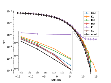
Figure 3: SER achieved in an AWGN channel by the proposed posterior probability estimators.

The second decoding problem is more challenging, as we consider a 4-PAM (i.e., pulse amplitude modulation) over a nonlinear channel with additive Gaussian noise. In particular, given the sequence of bits at time instant $t$ (referred to as $\mathbf{x}_{t}$), we obtain the channel output as

$$\mathbf{y}_{t}=H(\mathbf{x}_{t})=sgn(\mathbf{x}_{t})\sqrt{|\mathbf{x}_{t}|}+\mathbf{n}_{t},$$ (51)

where $\mathbf{n}_{t}$ is the Gaussian noise vector added at time instant $t$ and $sgn(\cdot)$ is the sign function. We show the SER achieved by the proposed estimators in Figure 4, together with the results of the maxL and the MAP Genie estimators. The MAP Genie estimator uses the knowledge of the channel nonlinearity in (51) to decode the received sequence of bits. In a nonlinear channel, the proposed list of posterior probability estimators performs better than the max likelihood estimator, achieving accuracy close to the optimal MAP Genie estimator.

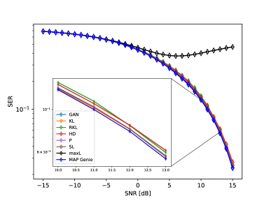
Figure 4: SER achieved by using a 4-PAM modulation over a nonlinear communication channel.

VII-D Continuous Posterior Estimation

This section comprises the two toy examples for the case $|\Omega|\geq|\mathbb{R}|$.

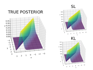
Figure 5: Posterior density estimation in the Gaussian task. The true posterior density is visualized on the left side. The posterior density estimate achieved with $\mathcal{J}_{SL}$ is showed in the top-right corner. The posterior density estimate achieved with $\mathcal{J}_{KL}$ is represented in the bottom-right corner.

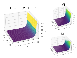
Figure 6: Posterior density estimation in the Exponential task. The true posterior density is visualized on the left side. The posterior density estimate achieved with $\mathcal{J}_{SL}$ is showed in the top-right corner. The posterior density estimate achieved with $\mathcal{J}_{KL}$ is represented in the bottom-right corner.

Gaussian task. In the first toy example, we consider the model $Y=X+N$, where $X\sim\mathcal{N}(0,\sigma_{X}^{2})$ and $N\sim\mathcal{N}(0,\sigma_{N}^{2})$ are independent random variables. Thus, $Y\sim\mathcal{N}(0,\underbrace{\sigma_{N}^{2}+\sigma_{X}^{2}}_{\triangleq\sigma_{Y}^{2}})$.
Then, the posterior density expression becomes

$$p_{X|Y}(x|y)=\frac{1}{\sqrt{2\pi}}\sqrt{\frac{\sigma_{Y}^{2}}{\sigma_{N}^{2}\sigma_{X}^{2}}}e^{-\frac{1}{2\sigma_{N}^{2}}\left[kx-\frac{y}{k}\right]^{2}},$$ (52)

where $k\triangleq\frac{\sigma_{X}^{2}+\sigma_{N}^{2}}{\sigma_{X}^{2}}$. The proof is reported in Appendix A-B.

The comparison between the closed-form of the posterior distribution and the discriminator estimate is showed in Figure 5, where $\sigma_{X}=1$ and $\sigma_{N}=\sigma_{X}/2$. The discriminator prediction is shown for two different cases. In the first case, reported in the upper-right corner, the network is trained using $\mathcal{J}_{SL}(D)$. In the second case, reported in the lower-right corner, the network is trained using $\mathcal{J}_{KL}(D)$. In both cases, the posterior probability estimate is accurate.

Exponential task. In the second toy example, we define the model $Y=X+N$, where $X\sim exp(\lambda)$ and $N\sim exp(\lambda)$ are independent random variables. Therefore, $Y\sim\Gamma(2,\frac{1}{\lambda})$ (i.e., a Gamma distribution with shape $2$ and rate $\frac{1}{\lambda}$) [40]. The posterior probability becomes (see Appendix A-B for the proof)

$$p_{X|Y}(x|y)=\frac{1}{y}\mathds{1}(x)\mathds{1}(y).$$ (53)

The comparison between the true posterior distribution and the estimate achieved by using the unsupervised objective function corresponding to SL and KL divergences is reported in Figure 6, where we fixed $\lambda=1$. The objective function corresponding to the SL divergence attains the best estimate. For a fixed $y$, in fact, the posterior density value is constant over $x$.

VIII Conclusions

In this paper, we proposed a new perspective for supervised classification problems. Casting the problem formulation in a Bayesian setting, we recognize the MAP criterion as the optimal solving approach. Therefore, we have proposed to use a discriminative formulation to express the posterior probability density, and we have derived two classes of estimators to estimate it. The first class of estimators is obtained by maximizing a class of objective functions that leverage the variational representation of well-known $f$-divergences. The second class of estimators is attained by maximizing a class of objective functions derived from the imposition of the convergence condition of the discriminator network. We compare a list of posterior probability estimators obtained from the two classes with the notorious cross-entropy minimization approach. Numerical results on different scenarios demonstrate the proposed estimators’ effectiveness and that the proposed SL divergence achieves the highest classification accuracy in almost all the scenarios. Additionally, we show that the proposed posterior probability estimators work for the general case of continuous pdf $p_{X}(\mathbf{x})$, for which we design a specific neural network architecture.

Appendix A Appendix

A-A Objective Functions Used in the Experiments

A-A1 Objective Functions Based on Well-Known $f$-Divergences

Table II reports the list of well-known $f$-divergences from which Table I derives. Let us call $f_{u}$ and $f_{u}^{*}$ the unsupervised generator function and its Fenchel conjugate in Table I, respectively. Differently, $f$ and $f^{*}$ are the supervised generator function and its Fenchel conjugate in Table II, respectively. Then,

$$f_{u}^{*}(t)=|\mathcal{T}_{x}|f^{*}(t),$$ (54)

where $|\mathcal{T}_{x}|$ is the Lebesgue measure of the support of $p_{X}(\mathbf{x})$. Accordingly,

$$f_{u}(u)=\sup_{t\in dom_{f_{u}^{*}}}\left\{ut-f_{u}^{*}(t)\right\}.$$ (55)

The usage of (54) is needed because $|\mathcal{T}_{x}|$ counterbalances the effect of $p_{U}(\mathbf{x})$. Thus, $|\mathcal{T}_{x}|$ is included in the expectation term computed over $p_{U}(\mathbf{x})$.
Vice versa, the supervised version of $f_{u}$ and $f_{u}^{*}$ can be easily attained by substituting $|\mathcal{T}_{x}|=1$.

The supervised and unsupervised objective functions used to achieve the results showed in Section VII are reported in this section.

TABLE II: $f$-divergences table. The corresponding $f$-divergences are: Kullback-Leibler, Reverse Kullback-Leibler, squared Hellinger distance, GAN, and Pearson $\chi^{2}$.

Name	$f(u)$	$f^{*}(t)$
KL	$u\log(u)$	$\exp{(t-1)}$
RKL	$-\log(u)$	$-1-\log(-t)$
HD	$(\sqrt{u}-1)^{2}$	$\frac{t}{1-t}$
GAN	$u\log(u)-(u+1)\log(u+1)$	$-\log(1-\exp{(t)})$
P	$(u-1)^{2}$	$\frac{1}{4}t^{2}+t$

Kullback-Leibler Divergence: The variational representation of the KL divergence is achieved substituting $f_{u,KL}^{*}$ listed in Table I in (1). This leads to the unsupervised objective function

$$\mathcal{J}_{KL}(D) =\operatorname{\mathbb{E}}_{(\mathbf{x},\mathbf{y})\sim p_{XY}(\mathbf{x},\mathbf{y})}\Bigl{[}\log(D(\mathbf{x},\mathbf{y}))\Bigr{]}$$

$$-\operatorname{\mathbb{E}}_{(\mathbf{x},\mathbf{y})\sim p_{U}(\mathbf{x})p_{Y}(\mathbf{y})}\Bigl{[}|\mathcal{T}_{x}|D(\mathbf{x},\mathbf{y})\Bigr{]}+1,$$ (56)

where $T^{\diamond}(\mathbf{x},\mathbf{y})=\log(\frac{p_{XY}(\mathbf{x},\mathbf{y})}{|\mathcal{T}_{x}|p_{U}(\mathbf{x})p_{Y}(\mathbf{y})})+1$, $p_{U}(\mathbf{x})=\frac{1}{|\mathcal{T}_{x}|}$, and $D^{\diamond}(\mathbf{x},\mathbf{y})=\frac{p_{XY}(\mathbf{x},\mathbf{y})}{p_{Y}(\mathbf{y})}$. The supervised version of the objective function in (A-A1) is attained by using Theorem 4:

$$\mathcal{J}_{KL}(D) =\operatorname{\mathbb{E}}_{\mathbf{x}\sim p_{X}(\mathbf{x})}\Biggl{[}\operatorname{\mathbb{E}}_{\mathbf{y}\sim p_{Y|X}(\mathbf{y}|\mathbf{x})}\Bigl{[}\log(\textbf{D}(\mathbf{y}))^{T}1_{m}(\mathbf{x})\Bigr{]}\Biggr{]}$$

$$-\operatorname{\mathbb{E}}_{\mathbf{y}\sim p_{Y}(\mathbf{y})}\Bigl{[}\textbf{D}(\mathbf{y})^{T}1_{m}\Bigr{]}.$$ (57)

When the last layer of the supervised discriminator utilizes the softmax activation function (i.e., when the output is normalized to be a probability mass function), then the second term in (A-A1) is always equal to 1. Thus, the maximization of (A-A1) exactly corresponds to the minimization of the KL divergence in (1), and therefore to the minimization of the cross-entropy.
Interestingly, the more general formulation in (A-A1) allows the usage of different activation functions in the last layer, with the only requirement that the discriminator’s output is constrained to assume positive values.

Reverse Kullback-Leibler Divergence: Theorem 1 leads to the variational representation of the reverse KL for classification problems, when substituting $f_{u,RKL}^{*}$ listed in Table I in (1)

$$\mathcal{J}_{RKL}(D) =\operatorname{\mathbb{E}}_{(\mathbf{x},\mathbf{y})\sim p_{XY}(\mathbf{x},\mathbf{y})}\Bigl{[}-D(\mathbf{x},\mathbf{y})\Bigr{]}$$

$$-\operatorname{\mathbb{E}}_{(\mathbf{x},\mathbf{y})\sim p_{U}(\mathbf{x})p_{Y}(\mathbf{y})}\Bigl{[}|\mathcal{T}_{x}|\log(D(\mathbf{x},\mathbf{y}))\Bigr{]},$$ (58)

where $T^{\diamond}(\mathbf{x},\mathbf{y})=-\frac{|\mathcal{T}_{x}|p_{U}(\mathbf{x})p_{Y}(\mathbf{y})}{p_{XY}(\mathbf{x},\mathbf{y})}$ and $D^{\diamond}(\mathbf{x},\mathbf{y})=\frac{p_{Y}(\mathbf{y})}{p_{XY}(\mathbf{x},\mathbf{y})}$. The supervised version of the objective function in (A-A1) is obtained by using Theorem 4.

$$\mathcal{J}_{RKL}(D) =\operatorname{\mathbb{E}}_{\mathbf{x}\sim p_{X}(\mathbf{x})}\Biggl{[}\operatorname{\mathbb{E}}_{\mathbf{y}\sim p_{Y|X}(\mathbf{y}|\mathbf{x})}\Bigl{[}-\textbf{D}(\mathbf{y})^{T}1_{m}(\mathbf{x})\Bigr{]}\Biggr{]}$$

$$-\operatorname{\mathbb{E}}_{\mathbf{y}\sim p_{Y}(\mathbf{y})}\Bigl{[}\log(\textbf{D}(\mathbf{y}))^{T}1_{m}\Bigr{]}.$$ (59)

Hellinger Squared Distance: Theorem 1 leads to the variational representation of the Hellinger squared distance for classification problems, when substituting $f_{u,HD}^{*}$ listed in Table I in (1)

$$\mathcal{J}_{HD}(D) =\operatorname{\mathbb{E}}_{(\mathbf{x},\mathbf{y})\sim p_{XY}(\mathbf{x},\mathbf{y})}\Bigl{[}-\sqrt{D(\mathbf{x},\mathbf{y})}\Bigr{]}$$

$$-\operatorname{\mathbb{E}}_{(\mathbf{x},\mathbf{y})\sim p_{U}(\mathbf{x})p_{Y}(\mathbf{y})}\Biggl{[}|\mathcal{T}_{x}|\frac{1}{\sqrt{D(\mathbf{x},\mathbf{y})}}\Biggr{]},$$ (60)

where $T^{\diamond}(\mathbf{x},\mathbf{y})=\left(\sqrt{\frac{p_{XY}(\mathbf{x},\mathbf{y})}{|\mathcal{T}_{x}|p_{U}(\mathbf{x})p_{Y}(\mathbf{y})}}-1\right)\sqrt{\frac{|\mathcal{T}_{x}|p_{U}(\mathbf{x})p_{Y}(\mathbf{y})}{p_{XY}(\mathbf{x},\mathbf{y})}}$, and $D^{\diamond}(\mathbf{x},\mathbf{y})=\frac{p_{Y}(\mathbf{y})}{p_{XY}(\mathbf{x},\mathbf{y})}$. The supervised implementation of the objective function in (A-A1) is achieved by using Theorem 4

$$\mathcal{J}_{HD}(D) =\operatorname{\mathbb{E}}_{\mathbf{x}\sim p_{X}(\mathbf{x})}\Biggl{[}\operatorname{\mathbb{E}}_{\mathbf{y}\sim p_{Y|X}(\mathbf{y}|\mathbf{x})}\Bigl{[}-\sqrt{\textbf{D}(\mathbf{y})}^{T}1_{m}(\mathbf{x})\Bigr{]}\Biggr{]}$$

$$-\operatorname{\mathbb{E}}_{\mathbf{y}\sim p_{Y}(\mathbf{y})}\Biggl{[}\left(\frac{1}{\sqrt{\textbf{D}(\mathbf{y})}}\right)^{T}1_{m}\Biggr{]}.$$ (61)

GAN: Theorem 1 leads to the variational representation of the GAN divergence for classification problems, when substituting $f_{u,GAN}^{*}$ listed in Table I in (1)

$$\mathcal{J}_{GAN}(D) =\operatorname{\mathbb{E}}_{(\mathbf{x},\mathbf{y})\sim p_{XY}(\mathbf{x},\mathbf{y})}\Bigl{[}\log(1-D(\mathbf{x},\mathbf{y}))\Bigr{]}$$

$$+\operatorname{\mathbb{E}}_{(\mathbf{x},\mathbf{y})\sim p_{U}(\mathbf{x})p_{Y}(\mathbf{y})}\Bigl{[}|\mathcal{T}_{x}|\log(D(\mathbf{x},\mathbf{y}))\Bigr{]},$$ (62)

where $T^{\diamond}(\mathbf{x},\mathbf{y})=\log{\left(\frac{p_{XY}(\mathbf{x},\mathbf{y})}{p_{XY}(\mathbf{x},\mathbf{y})+|\mathcal{T}_{x}|p_{U}(\mathbf{x})p_{Y}(\mathbf{y})}\right)}$ and $D^{\diamond}(\mathbf{x},\mathbf{y})=\frac{p_{Y}(\mathbf{y})}{p_{Y}(\mathbf{y})+p_{XY}(\mathbf{x},\mathbf{y})}$. The supervised implementation of the objective function in (A-A1) is

$$\mathcal{J}_{GAN}(D) =\operatorname{\mathbb{E}}_{\mathbf{x}\sim p_{X}(\mathbf{x})}\Biggl{[}\operatorname{\mathbb{E}}_{\mathbf{y}\sim p_{Y|X}(\mathbf{y}|\mathbf{x})}\Bigl{[}\log(1_{m}-\textbf{D}(\mathbf{y}))^{T}$$

$$\cdot 1_{m}(\mathbf{x})\Bigr{]}\Biggr{]}+\operatorname{\mathbb{E}}_{\mathbf{y}\sim p_{Y}(\mathbf{y})}\Bigl{[}\left(\log(\textbf{D}(\mathbf{y}))\right)^{T}1_{m}\Bigr{]}.$$

Pearson $\chi^{2}$: Theorem 1 leads to the variational representation of the Pearson $\chi^{2}$ divergence for classification problems, when substituting $f_{u,P}^{*}$ listed in Table I in (1)

$$\mathcal{J}_{P}(D) =\operatorname{\mathbb{E}}_{(\mathbf{x},\mathbf{y})\sim p_{XY}(\mathbf{x},\mathbf{y})}\Bigl{[}2(D(\mathbf{x},\mathbf{y})-1)\Bigr{]}$$

$$-\operatorname{\mathbb{E}}_{(\mathbf{x},\mathbf{y})\sim p_{U}(\mathbf{x})p_{Y}(\mathbf{y})}\Biggl{[}|\mathcal{T}_{x}|D^{2}(\mathbf{x},\mathbf{y})\Biggr{]},$$ (64)

where $T^{\diamond}(\mathbf{x},\mathbf{y})=2\left(\frac{p_{XY}(\mathbf{x},\mathbf{y})}{|\mathcal{T}_{x}|p_{U}(\mathbf{x})p_{Y}(\mathbf{y})}-1\right)$, and $D^{\diamond}(\mathbf{x},\mathbf{y})=\frac{p_{XY}(\mathbf{x},\mathbf{y})}{p_{Y}(\mathbf{y})}$. The supervised implementation of the objective function in (A-A1) is achieved by using Theorem 4

$$\mathcal{J}_{P}(D) =\operatorname{\mathbb{E}}_{\mathbf{x}\sim p_{X}(\mathbf{x})}\Biggl{[}\operatorname{\mathbb{E}}_{\mathbf{y}\sim p_{Y|X}(\mathbf{y}|\mathbf{x})}\Bigl{[}2(\textbf{D}(\mathbf{y})-1_{m})^{T}1_{m}(\mathbf{x})\Bigr{]}\Biggr{]}$$

$$-\operatorname{\mathbb{E}}_{\mathbf{y}\sim p_{Y}(\mathbf{y})}\Biggl{[}\left(\textbf{D}^{T}(\mathbf{y})\textbf{D}(\mathbf{y})\right)\Biggr{]}.$$ (65)

A-A2 Objective Functions of Shifted Log Divergence

The unsupervised and supervised versions of the objective function corresponding to the shifted log divergence are discussed in this paragraph.

Shifted log: Theorem 2 leads to the objective function in (3) when

$$k(p_{X|Y}(\mathbf{x}|\mathbf{y})) =\frac{|\mathcal{T}_{x}|p_{U}(\mathbf{x})p_{Y}(\mathbf{y})}{|\mathcal{T}_{x}|p_{U}(\mathbf{x})p_{Y}(\mathbf{y})+p_{XY}(\mathbf{x},\mathbf{y})}$$ (66)

$$g_{1}(D,k;1,0) =-\frac{|\mathcal{T}_{x}|p_{U}(\mathbf{x})p_{Y}(\mathbf{y})+p_{XY}(\mathbf{x},\mathbf{y})}{D(\mathbf{x},\mathbf{y})}.$$ (67)

Such an objective function is the variational representation of the shifted log divergence, where the generator function is reported in (34). We report it here for completeness

$$\mathcal{J}_{SL}(D) =-\operatorname{\mathbb{E}}_{(\mathbf{x},\mathbf{y})\sim p_{XY}(\mathbf{x},\mathbf{y})}\Bigl{[}D(\mathbf{x},\mathbf{y})\Bigr{]}$$

$$+\operatorname{\mathbb{E}}_{(\mathbf{x},\mathbf{y})\sim p_{U}(\mathbf{x})p_{Y}(\mathbf{y})}\Bigl{[}|\mathcal{T}_{x}|\Bigl{(}\log(D(\mathbf{x},\mathbf{y}))-D(\mathbf{x},\mathbf{y})\Bigr{)}\Bigr{]},$$ (68)

which can be obtained from Theorem 1 with $T^{\diamond}(\mathbf{x},\mathbf{y})=-\frac{|\mathcal{T}_{x}|p_{U}(\mathbf{x})p_{Y}(\mathbf{y})}{|\mathcal{T}_{x}|p_{U}(\mathbf{x})p_{Y}(\mathbf{y})+p_{XY}(\mathbf{x},\mathbf{y})}$ and $D^{\diamond}(\mathbf{x},\mathbf{y})=\frac{p_{Y}(\mathbf{y})}{p_{Y}(\mathbf{y})+p_{XY}(\mathbf{x},\mathbf{y})}$. The supervised implementation of the objective function in (A-A2) is achieved by using Theorem 4

$$\mathcal{J}_{SL}(D) =-\operatorname{\mathbb{E}}_{\mathbf{x}\sim p_{X}(\mathbf{x})}\Biggl{[}\operatorname{\mathbb{E}}_{\mathbf{y}\sim p_{Y|X}(\mathbf{y}|\mathbf{x})}\Bigl{[}\textbf{D}(\mathbf{y})^{T}1_{m}(\mathbf{x})\Bigr{]}\Biggr{]}$$

$$+\operatorname{\mathbb{E}}_{\mathbf{y}\sim p_{Y}(\mathbf{y})}\Bigl{[}\Bigl{(}\log(\textbf{D}(\mathbf{y}))-\textbf{D}(\mathbf{y})\Bigr{)}^{T}1_{m}\Bigr{]}.$$ (69)

A-B Proofs

Intuition of the Infeasibility of the Generalization of (1) as $f$-Divergence (see [16]). The gradient of (1) w.r.t. the model’s parameters can be easily computed, which makes feasible the minimization of (1). However, the generalization of the minimization of (1) with the $f$-divergence is not feasible. Let the general training objective be defined as

$$\min_{\theta}D_{f}(p||q_{\theta})=\min_{\theta}\operatorname{\mathbb{E}}_{q_{\theta}(\mathbf{x})}\Biggl{[}f\Bigl{(}\frac{p(\mathbf{x})}{q_{\theta}(\mathbf{x})}\Bigr{)}\Biggr{]},$$ (70)

where $p_{data}=p(\mathbf{x})$ and $p_{model}=q_{\theta}(\mathbf{x})$ to explicit its dependence on the model parameters. As an example, we consider the reverse KL (RKL), which is a member of the $f$-divergence family, i.e., $f_{RKL}(u)=-\log(u)$. Then, (70) becomes:

$$\min_{\theta}D_{RKL}(p||q_{\theta})=\min_{\theta}\operatorname{\mathbb{E}}_{q_{\theta}(\mathbf{x})}\Bigl{[}\log\Bigl{(}\frac{q_{\theta}(\mathbf{x})}{p(\mathbf{x})}\Bigr{)}\Bigr{]}.$$ (71)

The gradient calculation of (71) leads to

$$\nabla_{\theta}D_{RKL}(p||q_{\theta}) =\int_{\mathcal{X}}\nabla_{\theta}q_{\theta}(\mathbf{x})\Bigl{[}\log\left(\frac{q_{\theta}(\mathbf{x})}{p(\mathbf{x})}\right)+1\Bigr{]}d\mathbf{x}$$ (72)

$$=\operatorname{\mathbb{E}}_{q_{\theta}}\Bigl{[}\nabla_{\theta}\log q_{\theta}(\mathbf{x})\Bigl{(}\frac{q_{\theta}(\mathbf{x})}{p(\mathbf{x})}+1\Bigr{)}\Bigr{]},$$ (73)

where (73) is attained by noticing that $\nabla_{\theta}q_{\theta}(\mathbf{x})=q_{\theta}(\mathbf{x})\frac{\nabla_{\theta}q_{\theta}(\mathbf{x})}{q_{\theta}(\mathbf{x})}=q_{\theta}(\mathbf{x})\nabla_{\theta}\log q_{\theta}(\mathbf{x})$. As stated in [16], it is infeasible to estimate (73), since the density ratio $q_{\theta}(\mathbf{x})/p(\mathbf{x})$ is unknown.

Lemma 1.

Let $f(\cdot):\mathbb{R}\longrightarrow\mathbb{R}$ be the generator function of any $f$-divergence. Then, it holds:

$$(f^{*})^{\prime}(t)=(f^{{}^{\prime}})^{-1}(t)$$ (74)

Proof.

Let us recall the definition of Fenchel conjugate, to report a self-contained proof:

$$f^{*}(t)=\sup_{u\in\mathbb{R}}\left\{ut-f(u)\right\}.$$ (75)

Then, in order to find $u^{*}$ that achieves the supremum

$$\frac{\partial}{\partial u}\left\{ut-f(u)\right\}=0,$$ (76)

that implies

$$f^{{}^{\prime}}(u)=t.$$ (77)

Thus,

$$\hat{u}=(f^{{}^{\prime}})^{-1}(t)$$ (78)

Then, substituting (78) in the definition of the fenchel conjugate, it becomes:

$$f^{*}(t)=(f^{{}^{\prime}})^{-1}(t)t-f((f^{{}^{\prime}})^{-1}(t)).$$ (79)

Then, by computing the first derivative w.r.t. $t$:

$$(f^{*})^{{}^{\prime}}(t)=((f^{{}^{\prime}})^{-1})^{{}^{\prime}}(t)t+(f^{{}^{\prime}})^{-1}(t)-\underbrace{f^{{}^{\prime}}((f^{{}^{\prime}})^{-1}(t))}_{=t}((f^{{}^{\prime}})^{-1})^{{}^{\prime}}(t).$$ (80)

The first and third terms cancel out, leading to:

$$(f^{*})^{{}^{\prime}}(t)=(f^{{}^{\prime}})^{-1}(t).$$ (81)

∎

Corollary 2.1.

Let $\mathcal{J}(D)$ be defined as in Theorem 2. Let

$$k(p_{X|Y}(\mathbf{x}|\mathbf{y}))=k\left(\frac{p_{XY}(\mathbf{x},\mathbf{y})}{|\mathcal{T}_{x}|p_{U}(\mathbf{x})p_{Y}(\mathbf{y})}\right)=\frac{p_{0}}{p_{1}}.$$ (82)

Let define

$$g_{1}(D,k;\alpha,\beta)\triangleq-\frac{p_{1}}{D^{\alpha}}\left(\frac{1}{1-D}\right)^{\beta},$$ (83)

where $\alpha,\beta\in\mathbb{Q}$. Then, the objective functions in Table III are obtained from Theorem 2 by using $k(\cdot)$ and $g_{1}(\cdot)$ as defined in the set $\mathcal{F}_{k,g_{1}}\triangleq\{(k(x),(\alpha,\beta))_{f}\}$:

$$\mathcal{F}_{k,g_{1}}= \Biggl{\{}\Biggl{(}x,\left(1,0\right)\Biggr{)}_{KL},\Biggl{(}-\frac{1}{x},\left(1,0\right)\Biggr{)}_{RKL},$$

$$\Biggl{(}\frac{1}{x},\left(\frac{3}{2},0\right)\Biggr{)}_{HD},\Biggl{(}\frac{1}{1+x},\left(1,1\right)\Biggr{)}_{GAN},$$ (84)

$$\Biggl{(}x,(0,0)\Biggr{)}_{P}\Biggr{\}}$$ (85)

Proof.

Let rewrite for completeness

$$k_{KL}(p_{X|Y}(\mathbf{x}|\mathbf{y})) =p_{X|Y}(\mathbf{x}|\mathbf{y}),$$ (86)

$$k_{RKL}(p_{X|Y}(\mathbf{x}|\mathbf{y})) =-\frac{1}{p_{X|Y}(\mathbf{x}|\mathbf{y})},$$ (87)

$$k_{HD}(p_{X|Y}(\mathbf{x}|\mathbf{y})) =\frac{1}{p_{X|Y}(\mathbf{x}|\mathbf{y})},$$ (88)

$$k_{GAN}(p_{X|Y}(\mathbf{x}|\mathbf{y})) =\frac{1}{1+p_{X|Y}(\mathbf{x}|\mathbf{y})},$$ (89)

$$k_{P}(p_{X|Y}(\mathbf{x}|\mathbf{y})) =p_{X|Y}(\mathbf{x}|\mathbf{y}),$$ (90)

and

$$g_{1_{KL}}(D,k) =-\frac{p_{U}(\mathbf{x})p_{Y}(\mathbf{y})|\mathcal{T}_{x}|}{D(\mathbf{x},\mathbf{y})},$$ (91)

$$g_{1_{RKL}}(D,k) =\frac{p_{XY}(\mathbf{x},\mathbf{y})}{D(\mathbf{x},\mathbf{y})},$$ (92)

$$g_{1_{HD}}(D,k) =-\frac{p_{XY}(\mathbf{x},\mathbf{y})}{D^{\frac{3}{2}}(\mathbf{x},\mathbf{y})},$$ (93)

$$g_{1_{GAN}}(D,k) =-\frac{p_{U}(\mathbf{x})p_{Y}(\mathbf{y})|\mathcal{T}_{x}|+p_{XY}(\mathbf{x},\mathbf{y})}{D(\mathbf{x},\mathbf{y})(1-D(\mathbf{x},\mathbf{y}))},$$ (94)

$$g_{1_{P}}(D,k) =-p_{U}(\mathbf{x})p_{Y}(\mathbf{y})|\mathcal{T}_{x}|,$$ (95)

where the dependence of $g_{1}(\cdot)$ from $k$ is intrinsic in $p_{1}$. $g_{1}(\cdot)\neq 0$ because by definition each pdf is different from $0$ in its support. After a substitution in (2), they result

$$g_{KL}(D,k) =\frac{p_{XY}(\mathbf{x},\mathbf{y})}{D(\mathbf{x},\mathbf{y})}-p_{U}(\mathbf{x})p_{Y}(\mathbf{y})|\mathcal{T}_{x}|,$$ (96)

$$g_{RKL}(D,k) =-p_{XY}(\mathbf{x},\mathbf{y})-\frac{p_{Y}(\mathbf{y})}{D(\mathbf{x},\mathbf{y})},$$ (97)

$$g_{HD}(D,k) =-\frac{p_{XY}(\mathbf{x},\mathbf{y})}{\sqrt{D(\mathbf{x},\mathbf{y})}}+\frac{p_{U}(\mathbf{x})p_{Y}(\mathbf{y})}{\sqrt{D^{3}(\mathbf{x},\mathbf{y})}},$$ (98)

$$g_{GAN}(D,k) =\frac{p_{U}(\mathbf{x})p_{Y}(\mathbf{y})|\mathcal{T}_{x}|}{D(\mathbf{x},\mathbf{y})}-\frac{p_{XY}(\mathbf{x},\mathbf{y})}{1-D(\mathbf{x},\mathbf{y})},$$ (99)

$$g_{P}(D,k) =p_{XY}(\mathbf{x},\mathbf{y})-p_{U}(\mathbf{x})p_{Y}(\mathbf{y})|\mathcal{T}_{x}|D(\mathbf{x},\mathbf{y}).$$ (100)

After the integration w.r.t. $D$ and the substitution in (18), the objective functions in Table III are attained.

∎

Closed Form Posterior Gaussian Case: Let define the model $Y=X+N$, where $X\sim\mathcal{N}(0,\Sigma_{X})$, $N\sim\mathcal{N}(0,\Sigma_{N})$. Thus, $Y|X\sim\mathcal{N}(X,\Sigma_{N})$, $Y\sim\mathcal{N}(0,\underbrace{\Sigma_{N}+\Sigma_{X}}_{\triangleq\Sigma_{Y}})$.

The posterior probability is

$$p_{X|Y}(x|y) =\frac{p_{Y|X}(y|x)p_{X}(x)}{p_{Y}(y)}$$ (101)

$$=\frac{\frac{1}{\sqrt{(2\pi)^{d}|\Sigma_{N}|}}e^{-\frac{1}{2}(y-x)^{T}\Sigma_{N}^{-1}(y-x)}}{\frac{1}{\sqrt{(2\pi)^{d}|\Sigma_{Y}|}}e^{-\frac{1}{2}y^{T}\Sigma_{Y}^{-1}y}}$$

$$\cdot\frac{1}{\sqrt{(2\pi)^{d}|\Sigma_{X}|}}e^{-\frac{1}{2}x^{T}\Sigma_{X}^{-1}x}$$ (102)

$$=\frac{1}{\sqrt{(2\pi)^{d}}}\sqrt{\frac{|\Sigma_{Y}|}{|\Sigma_{N}||\Sigma_{X}|}}\exp\left\{-\frac{1}{2}G\right\},$$ (103)

where

$$G=x^{T}\Sigma_{x}^{-1}x+y^{T}\Sigma_{N}^{-1}y+x^{T}\Sigma_{N}^{-1}x-2x^{T}\Sigma_{N}^{-1}y-y^{T}\Sigma_{Y}^{-1}y.$$ (104)

In the scalar case, where $d=1$ and $\Sigma_{N}=\sigma_{N}^{2}$, $\Sigma_{X}=\sigma_{X}^{2}$ and $\Sigma_{Y}=\sigma_{X}^{2}+\sigma_{N}^{2}$, we have:

$$G =\frac{x^{2}}{\sigma_{X}^{2}}+\frac{y^{2}}{\sigma_{N}^{2}}+\frac{x^{2}}{\sigma_{N}^{2}}-2\frac{xy}{\sigma_{N}^{2}}-\frac{y^{2}}{\sigma_{y}^{2}}$$ (105)

$$=x^{2}\left(\frac{1}{\sigma_{X}^{2}}+\frac{1}{\sigma_{N}^{2}}\right)+y^{2}\left(\frac{1}{\sigma_{N}^{2}}-\frac{1}{\sigma_{Y}^{2}}\right)-\frac{2xy}{\sigma_{N}^{2}}$$ (106)

$$=x^{2}\left(\frac{\sigma_{X}^{2}+\sigma_{N}^{2}}{\sigma_{X}^{2}\sigma_{N}^{2}}\right)+y^{2}\left(\frac{\sigma_{Y}^{2}-\sigma_{N}^{2}}{\sigma_{N}^{2}\sigma_{Y}^{2}}\right)-\frac{2xy}{\sigma_{N}^{2}}$$ (107)

$$=\frac{1}{\sigma_{N}^{2}}\left[x^{2}\frac{\sigma_{N}^{2}+\sigma_{X}^{2}}{\sigma_{X}^{2}}+y^{2}\frac{\sigma_{x}^{2}}{\sigma_{X}^{2}+\sigma_{N}^{2}}-2xy\right]$$ (108)

$$=\frac{1}{\sigma_{N}^{2}}\left[x^{2}k^{2}+\frac{y^{2}}{k^{2}}-2xy\right]$$ (109)

$$=\frac{1}{\sigma_{N}^{2}}\left[kx-\frac{y}{k}\right]^{2},$$ (110)

where $k\triangleq\frac{\sigma_{X}^{2}+\sigma_{N}^{2}}{\sigma_{X}^{2}}>1$.

Closed Form Posterior Exponential Case: Let define the model $Y=X+N$, where $X\sim exp(\lambda)$, $N\sim exp(\lambda)$. Therefore, $Y\sim\Gamma(2,\frac{1}{\lambda})$ (i.e., a Gamma distribution with shape $2$ and rate $\frac{1}{\lambda}$). Let define $Y|X\triangleq Z$, then the cumulative density function (CDF) is

$$P\left[Z\leq z\right] =P\left[N+x_{c}\leq z\right]=P\left[N\leq z-x_{c}\right]$$

$$=\left(1-e^{-\lambda(z-x_{c})}\right)\mathds{1}(z-x_{c}),$$ (111)

where $X_{c}$ is constant. By deriving the CDF w.r.t. $z$, we compute the likelihood

$$p_{Y|X}(\mathbf{y}|\mathbf{x})=\lambda e^{-\lambda(y|x-x_{c})}\mathds{1}(y|x-x_{c})=p_{N}(n).$$ (112)

Then, the posterior probability is computed as

$$p_{X|Y}(x|y) =\frac{p_{N}(n)p_{X}(x)}{p_{Y}(y)}$$

$$=\frac{1}{y}\mathds{1}(x)\mathds{1}(y).$$ (113)

References

• [1] Mikaela Angelina Uy, Quang-Hieu Pham, Binh-Son Hua, Thanh Nguyen, and Sai-Kit Yeung. Revisiting point cloud classification: A new benchmark dataset and classification model on real-world data. In Proceedings of the IEEE/CVF international conference on computer vision, pages 1588–1597, 2019.
• [2] Yonghong Peng, Zhiqing Wu, and Jianmin Jiang. A novel feature selection approach for biomedical data classification. Journal of Biomedical Informatics, 43(1):15–23, 2010.
• [3] Eliya Nachmani, Elad Marciano, Loren Lugosch, Warren J. Gross, David Burshtein, and Yair Be’ery. Deep learning methods for improved decoding of linear codes. IEEE Journal of Selected Topics in Signal Processing, 12(1):119–131, 2018.
• [4] Stephen P Boyd and Lieven Vandenberghe. Convex optimization. Cambridge university press, 2004.
• [5] Yann LeCun, Yoshua Bengio, and Geoffrey Hinton. Deep learning. nature, 521(7553):436–444, 2015.
• [6] Nunzio A Letizia and Andrea M Tonello. Copula density neural estimation. arXiv preprint arXiv:2211.15353, 2022.
• [7] George Papamakarios, Theo Pavlakou, and Iain Murray. Masked autoregressive flow for density estimation. Advances in neural information processing systems, 30, 2017.
• [8] Shakir Mohamed and Balaji Lakshminarayanan. Learning in implicit generative models. arXiv preprint arXiv:1610.03483, 2016.
• [9] Karen Simonyan and Andrew Zisserman. Very deep convolutional networks for large-scale image recognition. In 3rd International Conference on Learning Representations, ICLR 2015, San Diego, CA, USA, May 7-9, 2015, Conference Track Proceedings, 2015.
• [10] Christian Szegedy, Wei Liu, Yangqing Jia, Pierre Sermanet, Scott Reed, Dragomir Anguelov, Dumitru Erhan, Vincent Vanhoucke, and Andrew Rabinovich. Going deeper with convolutions. In Proceedings of the IEEE conference on computer vision and pattern recognition, pages 1–9, 2015.
• [11] Edmar Rezende, Guilherme Ruppert, Tiago Carvalho, Fabio Ramos, and Paulo De Geus. Malicious software classification using transfer learning of resnet-50 deep neural network. In 2017 16th IEEE International Conference on Machine Learning and Applications (ICMLA), pages 1011–1014. IEEE, 2017.
• [12] Wei Tong, Weitao Chen, Wei Han, Xianju Li, and Lizhe Wang. Channel-attention-based densenet network for remote sensing image scene classification. IEEE Journal of Selected Topics in Applied Earth Observations and Remote Sensing, 13:4121–4132, 2020.
• [13] Srinadh Bhojanapalli, Ayan Chakrabarti, Daniel Glasner, Daliang Li, Thomas Unterthiner, and Andreas Veit. Understanding robustness of transformers for image classification. In Proceedings of the IEEE/CVF international conference on computer vision, pages 10231–10241, 2021.
• [14] Nataliia Kussul, Mykola Lavreniuk, Sergii Skakun, and Andrii Shelestov. Deep learning classification of land cover and crop types using remote sensing data. IEEE Geoscience and Remote Sensing Letters, 14(5):778–782, 2017.
• [15] Xiaofei Yang, Yunming Ye, Xutao Li, Raymond Y. K. Lau, Xiaofeng Zhang, and Xiaohui Huang. Hyperspectral image classification with deep learning models. IEEE Transactions on Geoscience and Remote Sensing, 56(9):5408–5423, 2018.
• [16] Lantao Yu, Yang Song, Jiaming Song, and Stefano Ermon. Training deep energy-based models with f-divergence minimization. In International Conference on Machine Learning, pages 10957–10967. PMLR, 2020.
• [17] Jiaheng Wei and Yang Liu. When optimizing $f$-divergence is robust with label noise. arXiv preprint arXiv:2011.03687, 2020.
• [18] Meiyu Zhong and Ravi Tandon. Learning fair classifiers via min-max f-divergence regularization. arXiv preprint arXiv:2306.16552, 2023.
• [19] Jiaming Song and Stefano Ermon. Understanding the limitations of variational mutual information estimators. In 8th International Conference on Learning Representations, ICLR 2020, Addis Ababa, Ethiopia, April 26-30, 2020, 2020.
• [20] Andrea M Tonello and Nunzio A Letizia. Mind: Maximum mutual information based neural decoder. IEEE Communications Letters, 26(12):2954–2958, 2022.
• [21] Nunzio A Letizia, Nicola Novello, and Andrea M Tonello. Variational $f$-divergence and derangements for discriminative mutual information estimation. arXiv preprint arXiv:2305.20025, 2023.
• [22] Sebastian Nowozin, Botond Cseke, and Ryota Tomioka. f-gan: Training generative neural samplers using variational divergence minimization. In D. Lee, M. Sugiyama, U. Luxburg, I. Guyon, and R. Garnett, editors, Advances in Neural Information Processing Systems, volume 29. Curran Associates, Inc., 2016.
• [23] XuanLong Nguyen, Martin J. Wainwright, and Michael I. Jordan. Estimating divergence functionals and the likelihood ratio by convex risk minimization. IEEE Transactions on Information Theory, 56(11):5847–5861, 2010.
• [24] Syed Mumtaz Ali and Samuel D Silvey. A general class of coefficients of divergence of one distribution from another. Journal of the Royal Statistical Society: Series B (Methodological), 28(1):131–142, 1966.
• [25] Imre Csiszár. On information-type measure of difference of probability distributions and indirect observations. Studia Sci. Math. Hungar., 2:299–318, 1967.
• [26] Sebastian Nowozin, Botond Cseke, and Ryota Tomioka. f-gan: Training generative neural samplers using variational divergence minimization. Advances in neural information processing systems, 29, 2016.
• [27] Nunzio A Letizia, Andrea M Tonello, and H Vincent Poor. Cooperative channel capacity learning. IEEE Communications Letters, 2023.
• [28] Igor Vajda. On the f-divergence and singularity of probability measures. Periodica Mathematica Hungarica, 2(1-4):223–234, 1972.
• [29] Pratik Chaudhari, Anna Choromanska, Stefano Soatto, Yann LeCun, Carlo Baldassi, Christian Borgs, Jennifer Chayes, Levent Sagun, and Riccardo Zecchina. Entropy-sgd: Biasing gradient descent into wide valleys. Journal of Statistical Mechanics: Theory and Experiment, 2019(12):124018, 2019.
• [30] Nitish Shirish Keskar, Dheevatsa Mudigere, Jorge Nocedal, Mikhail Smelyanskiy, and Ping Tak Peter Tang. On large-batch training for deep learning: Generalization gap and sharp minima. In ICLR, 2017.
• [31] Hao Li, Zheng Xu, Gavin Taylor, Christoph Studer, and Tom Goldstein. Visualizing the loss landscape of neural nets. Advances in neural information processing systems, 31, 2018.
• [32] David E Rumelhart, Geoffrey E Hinton, and Ronald J Williams. Learning representations by back-propagating errors. nature, 323(6088):533–536, 1986.
• [33] Diederik P. Kingma and Jimmy Ba. Adam: A method for stochastic optimization. In Yoshua Bengio and Yann LeCun, editors, 3rd International Conference on Learning Representations, ICLR 2015, San Diego, CA, USA, May 7-9, 2015, Conference Track Proceedings, 2015.
• [34] Nitish Srivastava, Geoffrey Hinton, Alex Krizhevsky, Ilya Sutskever, and Ruslan Salakhutdinov. Dropout: A simple way to prevent neural networks from overfitting. Journal of Machine Learning Research, 15(56):1929–1958, 2014.
• [35] Kaiming He, Xiangyu Zhang, Shaoqing Ren, and Jian Sun. Deep residual learning for image recognition. In Proceedings of the IEEE conference on computer vision and pattern recognition, pages 770–778, 2016.
• [36] Yann LeCun, Léon Bottou, Yoshua Bengio, and Patrick Haffner. Gradient-based learning applied to document recognition. Proceedings of the IEEE, 86(11):2278–2324, 1998.
• [37] Han Xiao, Kashif Rasul, and Roland Vollgraf. Fashion-mnist: a novel image dataset for benchmarking machine learning algorithms. arXiv preprint arXiv:1708.07747, 2017.
• [38] Alex Krizhevsky, Vinod Nair, and Geoffrey Hinton. The cifar-10 dataset. online: http://www. cs. toronto. edu/kriz/cifar. html, 55(5), 2014.
• [39] John G Proakis and Masoud Salehi. Fundamentals of communication systems. Pearson Education India, 2007.
• [40] Rick Durrett. Probability: theory and examples, volume 49. Cambridge university press, 2019.