Do Concept Bottleneck Models Obey Locality?

Abstract

Concept-based learning improves a deep learning model’s interpretability by explaining its predictions via human-understandable concepts. Deep learning models trained under this paradigm heavily rely on the assumption that neural networks can learn to predict the presence or absence of a given concept independently of other concepts. Recent work, however, strongly suggests that this assumption may fail to hold in Concept Bottleneck Models (CBMs), a quintessential family of concept-based interpretable architectures. In this paper, we investigate whether CBMs correctly capture the degree of conditional independence across concepts when such concepts are localised both spatially, by having their values entirely defined by a fixed subset of features, and semantically, by having their values correlated with only a fixed subset of predefined concepts. To understand locality, we analyse how changes to features outside of a concept’s spatial or semantic locality impact concept predictions. Our results suggest that even in well-defined scenarios where the presence of a concept is localised to a fixed feature subspace, or whose semantics are correlated to a small subset of other concepts, CBMs fail to learn this locality. These results cast doubt upon the quality of concept representations learnt by CBMs and strongly suggest that concept-based explanations may be fragile to changes outside their localities.

1 Introduction

Concept-based learning is an interpretability paradigm that leverages human-understandable concepts as a way to explain a deep learning model’s predictions [1, 2, 3, 4]. Concept Bottleneck Models (CBMs) [2] are constructed using this paradigm by first predicting concepts from an input sample and then using these concepts to predict a downstream label of interest. This design allows CBMs to: (1) provide concept-based explanations for their predictions via their predicted sets of concepts, and (2) improve their test performance when deployed in conjunction with experts via concept interventions [5, 6].

In this work, we investigate whether CBMs properly capture a task’s feature-to-concept and concept-to-concept relationships through the lens of what we will refer to as concept locality. Concept locality refers to the idea that, for certain tasks, a concept’s value is a function of a subset of features and concepts; modifications to features or concepts outside this should not impact the concept’s prediction. For example, the concept of “bird beak colour” should be predicted by focusing exclusively on the beak region of the image.

Recent work by Margeloiu et al. [7] has observed that features deemed important for a CBM’s concept’s prediction may not be confined to features known to fully define said concept. Here, we aim to build on this surprising result by analysing the locality of a CBM’s learnt concept representations when the training concepts are: (1) spatially localised, where values can be perfectly predicted from a well-defined subset of input features, and (2) semantically localised, where a concept’s value is independent of the value of a well-defined subset of concepts. We select these two modes to reflect varying granularities of features: spatial locality is related to changes in individual features, such as pixels, while semantic locality is related to changes to abstract-level groups of features (Figure 1).

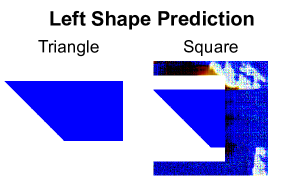
(a)

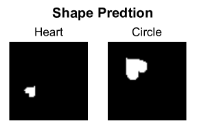
(b)

Figure 1: CBMs fail to accurately reflect localities present in tasks. (a) Changing pixels on the right side of the image modifies the prediction for the shape on the left side from a triangle to a square. (b) Rotation and dilation changes shape prediction from heart to circle.

Our contributions are the following: we (1) introduce spatial and semantic locality for concept-based models, (2) assess a CBM’s ability to capture the spatial locality and show this is inversely proportional to the CBM’s capacity, and (3) analyse a CBM’s ability to properly capture a task’s semantic locality and show that this is dependent on the task’s available concept annotations.

2 Related Works

Concept Learning

Concept learning [1, 8, 9, 10, 11, 3] is a subfield of eXplainable Artificial Intelligence (XAI) where a Deep Neural Network’s predictions are explained via high-level units of information (i.e., “concepts”). Methods in this field can vary from fully concept-supervised [2, 12, 4, 13], where one assumes access to both task and concept labels during training, to concept-unsupervised methods [9, 11, 14], where only task labels are available. In this paper, we explore Concept Bottleneck Models (CBMs) [2] due to their importance and ubiquity [3, 4, 13, 14, 15].

Robustness of Concept-Based Models

Since Margeloiu et al. [7] showed, via the use of saliency maps [16, 17, 18], that CBMs may construct their concept representations by possibly exploiting spurious correlations between concepts and input features, several works have studied this phenomenon [19, 20, 21, 22, 23, 24, 25]. Key amongst these, the work by Mahinpei et al. [19] stands out by showing how CBMs are prone to encoding undesired information in their learnt representations even when concepts are completely independent (referred to as “concept leakage”). This ignited several works attempting to understand how this leakage may be (1) detected at inference [22], (2) measured at test-time [20], (3) affected by a dataset’s inter-concept correlations [23], and (4) exploited for adversarial attacks against CBMs [21]. Our work differentiates itself from these by being the first to consider, to the best of our knowledge, how robust a CBM’s concept’s prediction is to changes entirely outside its spatial and semantic locality. Furthermore, we explore how elements often ignored during analysis, like the capacity of a CBM’s concept predictor, may play an essential part in the CBM’s robustness.

3 Introducing Locality

3.1 Concept Learning Setup

In the concept-supervised regime defined above, each training data point $\mathbf{x}$ has an associated set of $k$ binary concepts $\mathbf{c}\in\{0,1\}^{k}$. This set serves as a low-dimensional human-understandable representation that is relevant for a downstream task of interest. Formally, during training we are given a set of input data, $X=\{\mathbf{x}^{(i)}\in\mathbb{R}^{m}\}_{i=1}^{n}$, task labels $Y=\{y^{(i)}\in\{1,\cdots,L\}\}_{i=1}^{n}$, and concepts $C=\{\mathbf{c}^{(i)}\in\{0,1\}^{k}\}_{i=1}^{n}$. For each data point, $\mathbf{c}^{(i)}$ is a binary $k$-length vector where $\mathbf{c}^{(i)}_{j}$ denotes whether the $j$-th concept (e.g., “red fruit”) is present or not in $\mathbf{x}^{(i)}$.

Concept learning can be used to develop interpretable architectures where predictions are made using concepts. This is typically done through a Concept Bottleneck Model (CBM) [2], a two-stage model consisting of a concept predictor $g:\mathbf{x}\mapsto\hat{\mathbf{c}}$, and a label predictor $f:\hat{\mathbf{c}}\mapsto\hat{y}$. CBMs allow for interpretability by analysing concept values during prediction.

3.2 Defining Locality

Spatial Locality

To properly capture feature-to-concept relationships, it is desirable for a CBM’s concept predictor to learn how a concept is “spatially localised” with respect to input features. In this context, capturing spatial locality implies that a CBM’s prediction $\hat{\mathbf{c}}^{(i)}_{j}$ of concept $\mathbf{c}^{(i)}_{j}$’s activation value should depend only on a minimum set of features $\mathcal{L}_{j}(\mathbf{x}^{(i)})\subseteq\{1,\cdots,m\}$. This set of features, which we call the local region of concept $\mathbf{c}_{j}$ for $\mathbf{x}^{(i)}$, corresponds to the smallest set of input features that an oracle would need to predict $\mathbf{c}^{(i)}_{j}$ from $\mathbf{x}^{(i)}$. When properly captured, spatial locality implies that a CBM’s concept’s prediction should be conditionally independent of features outside the concept’s local region $\mathcal{L}_{j}(\mathbf{x}^{(i)})$. Capturing spatial locality can ensure the robustness of a CBM’s explanation so noise on spatially irrelevant features does not impact concept predictions.

Semantic Locality

A CBM’s prediction of concept $\mathbf{c}_{j}$ should be conditionally independent of the other concepts which lack a semantic relationship with $\mathbf{c}_{j}$. Correctly capturing this property, which we call semantic locality, implies that a CBM predicts concepts using only relevant relationships between concepts. For example, if a dataset contained examples where both green background and green feathers were present, such a correlation should not be embedded into the model unless it is semantically meaningful. Models failing to capture semantic locality could have their concept predictions impacted by irrelevant inter-concept relationships. For example, changes to a bird’s background should not lead to changes in prediction for bird species.

Semantic locality differs from spatial locality in its granularity; while spatial locality is a property of how individual feature perturbations impact concept predictions, semantic locality is a property of the inter-concept relationships and is a reflection of a relationship between groups of features.

3.3 Measuring Locality

We develop quantitative metrics for measuring how well a concept-based method captures spatial and semantic localities in a set of concept representations. We measure whether a model captures spatial locality by determining if a concept prediction by a concept-based method can be arbitrarily modified through targeted changes to input features outside that concept’s known local region. Formally, for an input $\mathbf{x}^{(i)}$ and concept $\mathbf{c}_{j}$, we perturb features outside of $\mathcal{L}_{j}(\mathbf{x}^{(i)})$, that is, $\{1,\cdots,m\}\setminus\mathcal{L}_{j}(\mathbf{x}^{(i)})$, to see if we can flip the prediction of concept $j$. Specifically, we aim to find an $\mathbf{x}^{\prime}\in\mathbb{R}^{m}$ so that $\forall a\in\mathcal{L}_{j}(\mathbf{x}^{(i)}),\;\mathbf{x}^{\prime}_{a}=\mathbf{x}^{(i)}_{a}$ while $|g(\mathbf{x}^{\prime})_{j}-g(\mathbf{x}^{(i)})_{j}|$ is maximised. To find such an $\mathbf{x}^{\prime}$, we use gradient ascent to maximise the difference in concept prediction when getting $\mathbf{x}^{\prime}$ as an input and compare it with its prediction for the same concept when receiving $\mathbf{x}^{(i)}$ as an input. This metric, which we call the spatial locality leakage $\mathcal{S}$, can be formally defined as

$$\mathcal{S}\big{(}g,\mathbf{x}^{(i)}\big{)}:=\frac{1}{k}\sum_{j=1}^{k}\Bigg{(}\max_{\begin{subarray}{c}\mathbf{x}^{\prime}\in\mathbb{R}^{m}\text{ s.t. }\\ \forall a\in\mathcal{L}_{j}(\mathbf{x}^{(i)}),\;\mathbf{x}^{\prime}_{a}=\mathbf{x}^{(i)}_{a}\end{subarray}}|g(\mathbf{x}^{\prime})_{j}-g(\mathbf{x}^{(i)})_{j}|\Bigg{)}$$ (1)

where $g(\mathbf{x}^{\prime})_{j}$ represents the prediction for concept $j$ for input $\mathbf{x}^{\prime}$. This value captures the ease of changing concept predictions by modifying an input $x^{(i)}$. Large spatial locality leakages imply modifications to irrelevant features could impact concept predictions.

To explore semantic locality, we analyse the Concept Out-of-Distribution Accuracy (CODA), which is the concept accuracy across data points when training a CBM on only a subset of concept combinations. Ideally, the presence or lack of semantically unrelated concepts should not impact the behaviour of the concept predictor. To measure whether this assumption holds, we compute the accuracy of the concept predictor for each concept $j$.

4 Spatial Locality Experiments

Experimental Setup

In this section, we evaluate whether spatial locality is correctly learned by CBMs with the help of multiple variants of a synthetic dataset. We consider a synthetic image dataset in which each sample is formed by $r\in\{1,2,4\}$ objects that are spatially localised (e.g., constrained to a subregion of the input space) and can be either a “square” or a “triangle”. Concepts in this situation refer to the presence of each shape in each localized region; for example, one concept is whether a square is present in the top right corner. We note that shapes in one region are independent of those in another, hence enabling us to measure whether CBMs correctly capture spatial locality. Using this dataset, we train CBMs while varying the concept predictor architecture to determine if spatial locality can be captured by different concept predictor models in a CBM. Specifically, we train CBMs that use either a convolutional neural networks (CNN) or a multi-layer perception (MLP) as their concept predictor $g$, and vary the size of these models (more details in Appendix A).

Impact of Model Size

We investigate whether CBMs, trained on a simple 1-object synthetic dataset with clear spatial locality in its concepts, can properly capture such locality as one varies concept predictor capacity. In Figure 2(a) we see that larger capacity concept predictors lead to more spatial locality leakage in CBMs when the concept predictor is a CNN-based model. These results suggest that increasing the number of layers, and hence increasing the model’s capacity and parameters, may surprisingly lead to CBMs failing to correctly capture a task’s spatial locality.

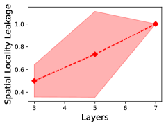
Figure 2: In tasks with spatial locality, CBM models fail to obey this locality. For the 1-object synthetic dataset, increasing the number of layers results in models that are not spatially localised.

We analyse this trend in MLP models in Appendix B and find similar patterns with model width, although the impact on a CBM’s ability to capture spatial locality as we change the capacity of its MLP concept predictor is less clear. To alleviate this problem, we find that pruning models then briefly retraining improves spatial locality; we provide further details in Appendix C.

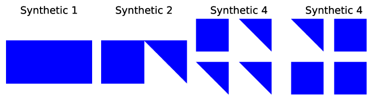
Figure 6: We plot examples of the synthetic dataset with 1, 2, and 4 objects. We note that for the 1-object synthetic dataset, the only relevant object for concept predictors is on the left side, while the right side is essentially noise.

Prior work argued that larger models could memorise more spurious correlations, which provides an intuition for why spatial locality is worse with larger models [26]. Such an explanation might also apply to our scenario, as the extra capacity allows concept predictor models to learn irrelevant features. Nevertheless, as shown in Figure 6 of our Appendix, our synthetic dataset is built so that concepts are localised to one and only one region independently of concepts in different regions. Therefore, these results cast a serious concern on what sorts of relationships and correlations a CBM’s concept predictor may be capturing in practice when predicting a concept. Perhaps more importantly, these results are not restricted to CBMs: in Appendix G we show that training concept predictors independent of the downstream task still lead to spatial locality leakage.

CUB Experiments

To understand if models are spatially localised in situations where a concept’s local region is not always fully known/clear, we investigate how concept predictions change when masking relevant and irrelevant features. We run experiments masking various concepts using the Caltech-UC Davis Birds (CUB) dataset [27], which consists of images of birds annotated with several visual properties (i.e., “concepts”) as well as with the type of species they belong to. The concepts in this dataset are different bird attributes, such as beak colour, tail length, and wing colour. Each concept is part of a concept group, which we denote $r(j)$: the group for concept $\mathbf{c}_{j}$; the concepts “beak red colour” and “beak blue colour” are in the same concept group. We are given the centre of each concept group for each data point, which we denote as $t_{r(j)}(\mathbf{x})\in\mathbb{R}_{+}^{2}$. We consider the local region for the concept to be within a distance $\epsilon$ of this centre, where $\epsilon$ is normalised with respect to the image width. We generate a mask within a distance $\epsilon$ of the centre and measure the average change in concept predictions within the concept group as a result of this mask (example in Figure 3).

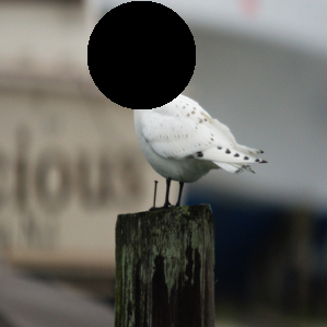
(a)

(b)

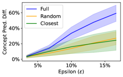
(c)

Figure 3: We compare examples of full masking (a) and closest masking (b) for the part “crown”, referring to the top of the bird’s head. We note that the closest masking only covers the top of the bird’s head, while the full masking covers other parts, such as parts of the feathers and neck. (c) Full masks lead to larger concept changes than closest masks, so, for example, masking out the neck of a bird impacts predictions for its head colour.

To investigate input-concept locality, we construct a spatial locality mask $\mathbf{\mu}_{j}\in\{0,1\}^{m}$ for each concept $\mathbf{c}_{j}$ that selects a combination of relevant and irrelevant features for its corresponding concept. For simplicity, for all concepts $\mathbf{c}_{j}$ we constrain $\mathbf{\mu}_{j}$ to be a circular mask with radius $\epsilon$, selected as a hyperparameter, and a different centre selected via the following policies:

1. Full - $\mathbf{\mu}_{j}$ is centred at $t_{r(j)}(\mathbf{x})$, the known annotated centre of its concept group.

2. Closest - $\mathbf{\mu}_{j}$ is centred at $t_{r(j)}(\mathbf{x})$ but we include only pixels that are closer to concept $\mathbf{c}_{j}$’s centre than the centre of any other concept. That is, we select all points $\mathbf{p}\in\mathbb{R}_{+}^{2}$ so that $||\mathbf{p}-t_{r(j)}(\mathbf{x})||_{2}\leq\epsilon$ and $\forall j^{\prime}\neq j,\;||\mathbf{p}-t_{r(j)}(\mathbf{x})||_{2}\leq||\mathbf{p}-t_{r(j^{\prime})}(\mathbf{x})||_{2}$.

3. Random - $\mathbf{\mu}_{j}$ is centred at a random location.

Our results, shown in Figure 3(c), suggest that concepts learnt by a CBM are not spatially localised to their respective part. While increasing the mask radius $\epsilon$ results in changes for concept prediction, we see that using full masking results in much larger changes to the concept prediction than either the random or closest masks. The difference between full and closest masking is that full masking covers pixels associated with other concept groups, and so masking these pixels out results in a large change for the concept predictions. For example, modifying pixels associated with the “neck” part impacts the prediction for “crown colour”.

Essentially, modifying pixels closer to other concept groups, which represent different body parts, leads to significantly different predictions for a given concept. One consequence of these results is that partially occluded concepts might leverage other independent regions to make predictions. These results highlight that CBMs fail to capture spatial locality even in real-world tasks, as their concept predictors may exploit pixels outside the spatially local region.

5 Semantic Locality Experiments

Experimental Setup

To investigate whether CBMs capture semantic locality, we explore synthetic tasks built using the dSprites dataset [28]. The dataset consists of various semantically independent attributes, including “position”, “size”, “colour”, and “shape”. We split each of these attributes into various concepts, resulting in $288$ unique concept combinations, and use $20$ for training, then evaluate across all combinations at test time (more details in Appendix E).

Concept-to-concept Interactions

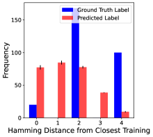
Figure 4: Frequency of Hamming distances between a CBM’s concept predictions, $\hat{\mathbf{c}}$, on the dSprites test set and the closest training concept annotation $\mathbf{c}$. Smaller hamming distances indicate predictions are closer to the training dataset. Predictions are closer to the training set than concept annotations, showing that concept predictors struggle beyond the training dataset.

To understand if semantically unrelated concepts can impact concept predictions, we measure whether novel concept combinations in the testing set lead CBMs to change their concept predictions. While concept predictors should be able to make predictions dissimilar to concept combinations seen during training, in Figure 4 we find that this is not true. CBMs tend to generate concept combinations already seen in the training dataset, as most predictions have a small Hamming distance to training data points. These results show the tendency of CBM models to memorise training explanations, revealing a lack of semantic locality. To account for confounding factors, we vary concept predictor capacity and training set size in Appendix D, finding that larger training sets improve concept accuracy slightly.

Model Generalisation

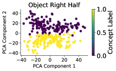
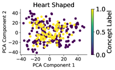
Figure 5: PCA projection of images from the dSprites dataset and their labels predicted by the SVM. Notice how the “Right Half” concept is linearly separable while the “Heart” concept is not.

To better understand why concept combinations have these differences, we use Principal Component Analysis (PCA) to project inputs into 2D [29] and use a linear SVM to predict concepts. In Figure 5 we display concept predictions for two concepts: one (“right half”) which has linear separability and is easier to predict, while another (“heart shaped”) lacks linear separability and is harder to predict. At an individual concept level, we see that the accuracy of the SVM on the dimensionality-reduced dataset, which we denote PCA accuracy, varies significantly amongst concepts. In Figure 9, we find that data which results in higher PCA accuracy leads to better CODA, indicating that more difficult concepts are harder to predict when faced with new concept combinations (see Appendix F). This implies that the issues are with the inability of concept predictors to learn meaningful relationships: even when training these concept predictors independently, they only achieve 8% task accuracy (see Appendix G). In future work, we plan to explore novel forms of regularisation for concept predictors that encourage concept predictions to better capture independence and semantic locality.

6 Conclusion and Future Work

In this paper, we explored whether CBMs can properly learn two types of locality found in concept-annotated datasets: spatial and semantic. These notions of locality capture whether a CBM learns to use only relevant feature-to-concept and concept-to-concept relationships. We find that spatial locality risks being miscaptured when a CBM’s concept predictor is overparameterised, while semantic locality is impacted by the diversity of training concept annotations. These findings demonstrate that small changes in the training set and architecture can impact the quality of a CBM’s explanations. In future work, we will explore whether recent methods developed for adversarial and spurious robustness in CBMs [21, 23] can lead to CBMs capturing locality better.

Appendix A Synthetic Dataset Setup Details

We develop a synthetic dataset to understand spatial locality. For this dataset, we define 3 sizes of images, of size $1$, $2$, and $4$, with the 1-object synthetic dataset containing 2 objects, but only having concept information on the first concept. We set the same task label for all data points, as we focus on concept predictors, and we want to avoid interference between the label and concept predictors. We note that each concept corresponds to an object, and so the relevant features for each concept correspond to the region in which the object resides. For all spatial locality experiments, we consider five trials for the input image $\mathbf{x}^{(i)}$ when computing the spatial locality leakage.

We find that all models learn the training data perfectly, achieving 100% concept accuracy and label accuracy across the train and test datasets. We train CBMs that use a convolutional neural network (CNN) as their concept predictor $g$ and test the impact of depth upon spatial locality by varying the number of convolutional layers in $\{3,5,7\}$. We additionally test CBMs that use a multi-layer perceptron (MLP) model as their concept predictors $g$ while varying the number of hidden layers across $\{1,2,3\}$ and the layer width across $\{5,10,15\}$. We consider the impact of other factors, such as the optimizer, weighting of the concept and task loss terms, and the introduction of noise to the dataset, and find that these factors do not impact the presence of spatial locality. Across all experiments, we train all models over three distinct random seeds and report the means and standard deviations of all metrics of interest.

Appendix B MLP Model Size

Depth	Width	Leakage
1	5	0.67 $\pm$ 0.32
	10	0.78 $\pm$ 0.32
	15	0.90 $\pm$ 0.14
2	5	0.64 $\pm$ 0.26
	10	0.61 $\pm$ 0.29
	15	0.64 $\pm$ 0.26
3	5	0.61 $\pm$ 0.07
	10	0.41 $\pm$ 0.07
	15	0.97 $\pm$ 0.04

Table 1: Increasing the width of models leads to increases in spatial locality leakage for depth 1 and 3 models, while there is no pattern in depth 2 models. Additionally, no such pattern is seen when increasing the depth of models, showing that the width of a model might be more responsible for spatial locality leakage than its depth.

We study whether MLP models capture spatial locality, as they present a controlled scenario where the parameter size, along with depth and width, can be varied arbitrarily. For MLP-based concept predictors, we see that when using a single hidden layer we observe an increase in spatial locality leakage as we increase the width of the hidden layer (Table 1). This trend is similar to the one exhibited in CNN concept predictors, where larger models lead to more spatial locality leakage. However, unexpectedly, we also find that when the model width is fixed, and the number of hidden layers is increased, the amount of spatial locality leakage does not necessarily increase. The reason for this is unclear; it might be due to the small hidden layer sizes creating an information bottleneck [30], where information gets compressed when travelling between layers.

Appendix C CNN Pruning Experiments

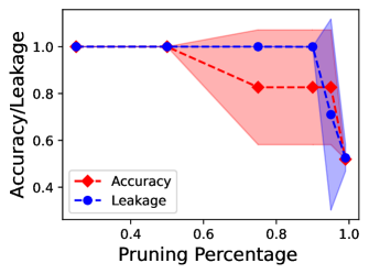
(a)

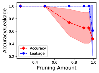
(b)

Figure 7: We prune CNN-based concept predictors using layer and weight pruning without retraining. We find that for both pruning strategies, accuracy significantly drops off before spatial locality leakage does, making it difficult to remove spatial locality leakage simply through pruning.

If model size is responsible for spatially local leakage, then model pruning offers a potential solution to reduce model size and address spatial locality leakage. We consider two types of pruning: layer pruning and weight pruning [31]. In layer pruning, we prune a constant percentage of the filters in each layer, pruning filters that have the lowest weight, while in weight pruning, we globally prune a constant percentage of the weights based on weight norm, setting these to zero. We note that for each type of pruning, we don’t retrain after pruning. In Figure 7, we see that increasing the pruning percentage decreases accuracy and spatial locality leakage for both layer and weight pruning. However, for both of these, we see that accuracy decreases before the spatial locality leakage does. In other words, pruning CNN models results in significantly decreased accuracy before spatial locality leakage is, and so pruning large models into small ones isn’t a viable strategy to eliminate spatial locality leakage.

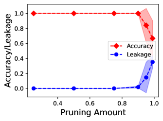
Figure 8: Using weight pruning then retraining models for 1 epoch leads to models with high accuracy and low spatial locality leakage. This presents a viable strategy to remove spatial locality leakage in large models.

To improve accuracy while leveraging pruning, we retrain models for 1 epoch after pruning. In Figure 8, we see that retraining models after weight pruning leads to high accuracy with low spatial locality leakage. Pruning then retraining provides a viable strategy to improve the spatial locality leakage of models while preserving the accuracy, though provides additional training burdens. We plan to investigate whether such trends hold when using non-synthetic datasets.

Appendix D Concept Combinations

Concept Combinations	CODA
5	58% $\pm$ 0%
10	63% $\pm$ 0%
15	65% $\pm$ 0%
20	64% $\pm$ 1%

Table 2: Increasing the number of concept combinations leads to higher CODA, though this increases at a slow, sublinear rate.

To better understand semantic locality, we vary the number of training concept combinations (Table 2). We randomly select $5$, $10$, $15$, and $20$ concept combinations, and train models based on these concept combinations. As expected, more concept combinations lead to higher CODA. However, such a trend is relatively slow, as changing the number of concept combinations from $5$ to $20$, a 4x increase, only improves accuracy by $6\%$. Therefore, simply increasing the size of the dataset is not sufficient to prevent this issue.

Appendix E Semantic Locality Dataset

We describe our semantic locality dataset and our setup for the semantic locality experiments. We use the dSprites dataset for the semantic locality experiments [28]. The dSprites dataset consists of images of an object with varying locations, shapes, and sizes. We divide the location into 2 concepts for the x position and 2 concepts for the y position. We additionally divide the shape into 3 concepts, one each for “heart”, “circle”, and “square.” We have one concept for the colour, as the colour is constant across all images. We have four concepts for the rotation, and six concepts for the size, resulting in 18 total concepts. The task is then to predict the base 2 representation of the concept, mod 100; essentially the task forces label predictors to have perfect knowledge of concepts, as the label relies on all concept values. We note that CBMs achieve perfect concept and task accuracy on the training set.

Appendix F Further Analysis of Semantic Locality

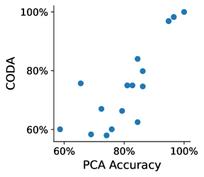
Figure 9: We compute the PCA accuracy using SVM models on the dimensionality reduced dSprites data for each concept, and compare it with the CODA, which is the accuracy on the test set when training with only a subset of concept combinations. We see that when the PCA accuracy is perfect, there also tends to be perfect CODA, while imperfect concepts lead to poor generalization.

Concept predictor models tend to predict concept combinations already found in training data, which is indicative of accuracy issues for concepts. In Figure 9, we compare the CODA, which is the performance of concept predictors across all concept combinations, with the corresponding PCA accuracy, which is the accuracy predicted just using the SVM on dimensionality-reduced testing points. We see that concepts with perfect PCA accuracy when predicted using dimensionality-reduced data, tend to have a high CODA, while those with imperfect concept accuracies have CODA as low as $6\%$. This relationship matches with intuition, as perfectly predicted concepts tend to not be impacted by the predictions of other concepts, leading to a high CODA. Because many concepts have a low CODA, the overall task accuracy is 3%; the low task accuracy is in contrast to other concepts-based scenarios, as predicting task labels accurately requires perfect knowledge of concepts, which isn’t true for other concept-based datasets [27]. By constructing our dataset so concept combinations in the training are not representative of testing, we reveal that concept predictors erroneously pick up on relationships between semantically independent concepts.

Appendix G Using Independent Models

We compare the locality properties when using independent models instead of joint models when training CBMs. Independent models are trained by training the concept predictor and label predictor separately, so that leakage between the task label and concept label is prevented. By training with independent models, we investigate whether leakage between the task label and concept label is responsible for the lack of locality exhibited by some models in the spatial and semantic locality scenarios.

With spatial locality, we find that the results are unchanged when using independent models. We test out independent models on the $7$ layer concept predictor. Originally, we found that all models had spatial locality leakage of $1$ across all runs. We find that the same trend is repeated in the independent model case; all models exhibit a spatial locality leakage of $1$ .

With the semantic locality case, we find that the overall task accuracy improves from 3% to 8%. While this improvement is positive, CBM models are still unable to consistently predict correct labels, which is reflective of issues with the concept predictor. We intend to investigate this further in future work.

Appendix H Masking experiment Details

We provide details on our experiment involves various masks with the CUB dataset. We aim to see if the type of maksing impacts concept prediction. For our concept predictor, we use a three-layer CNN, then construct a mask for each concept, for each of three different seeds, and for $\epsilon$ across $\{3.3\%,6.6\%,10\%,13.3\%,16.6\%\}$. We then compute the average concept change for a given concept group $r(j)$, with a non-masked input $x$ and a masked input $x^{\prime}$ as:

$$\frac{1}{\sum_{j^{\prime}=1,r(j)=r(j^{\prime})}^{k}1}\sum_{j^{\prime}=1,r(j)=r(j^{\prime})}^{k}|g(x)_{j^{\prime}}-g(x^{\prime})_{j^{\prime}}|$$ (2)

We then average this across all concept groups and random seeds.

References

- Kim et al. [2018] Been Kim, Martin Wattenberg, Justin Gilmer, Carrie Cai, James Wexler, Fernanda Viegas, et al. Interpretability beyond feature attribution: Quantitative testing with concept activation vectors (tcav). In International conference on machine learning, pages 2668–2677. PMLR, 2018.
- Koh et al. [2020] Pang Wei Koh, Thao Nguyen, Yew Siang Tang, Stephen Mussmann, Emma Pierson, Been Kim, and Percy Liang. Concept bottleneck models. In International Conference on Machine Learning, pages 5338–5348. PMLR, 2020.
- Espinosa Zarlenga et al. [2022] Mateo Espinosa Zarlenga, Pietro Barbiero, Gabriele Ciravegna, Giuseppe Marra, Francesco Giannini, Michelangelo Diligenti, Zohreh Shams, Frederic Precioso, Stefano Melacci, Adrian Weller, et al. Concept embedding models: Beyond the accuracy-explainability trade-off. Advances in Neural Information Processing Systems, 35:21400–21413, 2022.
- Yuksekgonul et al. [2022] Mert Yuksekgonul, Maggie Wang, and James Zou. Post-hoc concept bottleneck models. arXiv preprint arXiv:2205.15480, 2022.
- Chauhan et al. [2022] Kushal Chauhan, Rishabh Tiwari, Jan Freyberg, Pradeep Shenoy, and Krishnamurthy Dvijotham. Interactive concept bottleneck models. arXiv preprint arXiv:2212.07430, 2022.
- Shin et al. [2023] Sungbin Shin, Yohan Jo, Sungsoo Ahn, and Namhoon Lee. A closer look at the intervention procedure of concept bottleneck models. arXiv preprint arXiv:2302.14260, 2023.
- Margeloiu et al. [2021] Andrei Margeloiu, Matthew Ashman, Umang Bhatt, Yanzhi Chen, Mateja Jamnik, and Adrian Weller. Do concept bottleneck models learn as intended? arXiv preprint arXiv:2105.04289, 2021.
- Goyal et al. [2019] Yash Goyal, Amir Feder, Uri Shalit, and Been Kim. Explaining classifiers with causal concept effect (cace). arXiv preprint arXiv:1907.07165, 2019.
- Ghorbani et al. [2019] Amirata Ghorbani, James Wexler, James Y Zou, and Been Kim. Towards automatic concept-based explanations. Advances in Neural Information Processing Systems, 32, 2019.
- Kazhdan et al. [2020] Dmitry Kazhdan, Botty Dimanov, Mateja Jamnik, Pietro Liò, and Adrian Weller. Now you see me (cme): concept-based model extraction. arXiv preprint arXiv:2010.13233, 2020.
- Yeh et al. [2020] Chih-Kuan Yeh, Been Kim, Sercan Arik, Chun-Liang Li, Tomas Pfister, and Pradeep Ravikumar. On completeness-aware concept-based explanations in deep neural networks. Advances in Neural Information Processing Systems, 33:20554–20565, 2020.
- Chen et al. [2020] Zhi Chen, Yijie Bei, and Cynthia Rudin. Concept whitening for interpretable image recognition. Nature Machine Intelligence, 2(12):772–782, 2020.
- Kim et al. [2023] Eunji Kim, Dahuin Jung, Sangha Park, Siwon Kim, and Sungroh Yoon. Probabilistic concept bottleneck models. arXiv preprint arXiv:2306.01574, 2023.
- Oikarinen et al. [2023] Tuomas Oikarinen, Subhro Das, Lam M Nguyen, and Tsui-Wei Weng. Label-free concept bottleneck models. arXiv preprint arXiv:2304.06129, 2023.
- Zarlenga et al. [2023] Mateo Espinosa Zarlenga, Zohreh Shams, Michael Edward Nelson, Been Kim, and Mateja Jamnik. Tabcbm: Concept-based interpretable neural networks for tabular data. Transactions on Machine Learning Research, 2023.
- Baehrens et al. [2010] David Baehrens, Timon Schroeter, Stefan Harmeling, Motoaki Kawanabe, Katja Hansen, and Klaus-Robert Müller. How to explain individual classification decisions. The Journal of Machine Learning Research, 11:1803–1831, 2010.
- Smilkov et al. [2017] Daniel Smilkov, Nikhil Thorat, Been Kim, Fernanda Viégas, and Martin Wattenberg. Smoothgrad: removing noise by adding noise. arXiv preprint arXiv:1706.03825, 2017.
- Sundararajan et al. [2017] Mukund Sundararajan, Ankur Taly, and Qiqi Yan. Axiomatic attribution for deep networks. In International conference on machine learning, pages 3319–3328. PMLR, 2017.
- Mahinpei et al. [2021] Anita Mahinpei, Justin Clark, Isaac Lage, Finale Doshi-Velez, and Weiwei Pan. Promises and pitfalls of black-box concept learning models. arXiv preprint arXiv:2106.13314, 2021.
- Espinosa Zarlenga et al. [2023] Mateo Espinosa Zarlenga, Pietro Barbiero, Zohreh Shams, Dmitry Kazhdan, Umang Bhatt, Adrian Weller, and Mateja Jamnik. Towards Robust Metrics for Concept Representation Evaluation. Proceedings of the AAAI Conference on Artificial Intelligence, 37(10):11791–11799, June 2023. doi: 10.1609/aaai.v37i10.26392. URL https://ojs.aaai.org/index.php/AAAI/article/view/26392.
- Sinha et al. [2023] Sanchit Sinha, Mengdi Huai, Jianhui Sun, and Aidong Zhang. Understanding and enhancing robustness of concept-based models. In Proceedings of the AAAI Conference on Artificial Intelligence, volume 37, pages 15127–15135, 2023.
- Marconato et al. [2022a] Emanuele Marconato, Andrea Passerini, and Stefano Teso. Glancenets: Interpretable, leak-proof concept-based models. Advances in Neural Information Processing Systems, 35:21212–21227, 2022a.
- Heidemann et al. [2023] Lena Heidemann, Maureen Monnet, and Karsten Roscher. Concept correlation and its effects on concept-based models. In Proceedings of the IEEE/CVF Winter Conference on Applications of Computer Vision, pages 4780–4788, 2023.
- Havasi et al. [2022] Marton Havasi, Sonali Parbhoo, and Finale Doshi-Velez. Addressing leakage in concept bottleneck models. Advances in Neural Information Processing Systems, 35:23386–23397, 2022.
- Marconato et al. [2022b] Emanuele Marconato, Andrea Passerini, and Stefano Teso. Glancenets: Interpretable, leak-proof concept-based models. Advances in Neural Information Processing Systems, 35:21212–21227, 2022b.
- Sagawa et al. [2020] Shiori Sagawa, Aditi Raghunathan, Pang Wei Koh, and Percy Liang. An investigation of why overparameterization exacerbates spurious correlations. In International Conference on Machine Learning, pages 8346–8356. PMLR, 2020.
- Wah et al. [2011] Catherine Wah, Steve Branson, Peter Welinder, Pietro Perona, and Serge Belongie. The caltech-ucsd birds-200-2011 dataset. 2011.
- Matthey et al. [2017] Loic Matthey, Irina Higgins, Demis Hassabis, and Alexander Lerchner. dsprites: Disentanglement testing sprites dataset. https://github.com/deepmind/dsprites-dataset/, 2017.
- F.R.S. [1901] Karl Pearson F.R.S. Liii. on lines and planes of closest fit to systems of points in space. The London, Edinburgh, and Dublin Philosophical Magazine and Journal of Science, 2(11):559–572, 1901. doi: 10.1080/14786440109462720.
- Tishby et al. [2000] Naftali Tishby, Fernando C. Pereira, and William Bialek. The information bottleneck method, 2000.
- Blalock et al. [2020] Davis Blalock, Jose Javier Gonzalez Ortiz, Jonathan Frankle, and John Guttag. What is the state of neural network pruning? Proceedings of machine learning and systems, 2:129–146, 2020.