Contrastive Sequential Interaction Network Learning on Co-Evolving Riemannian Spaces

Abstract

The sequential interaction network usually find itself in a variety of applications, e.g., recommender system. Herein, inferring future interaction is of fundamental importance, and previous efforts are mainly focused on the dynamics in the classic zero-curvature Euclidean space. Despite the promising results achieved by previous methods, a range of significant issues still largely remains open: On the bipartite nature, is it appropriate to place user and item nodes in one identical space regardless of their inherent difference? On the network dynamics, instead of a fixed curvature space, will the representation spaces evolve when new interactions arrive continuously? On the learning paradigm, can we get rid of the label information costly to acquire? To address the aforementioned issues, we propose a novel Contrastive model for Sequential Interaction Network learning on Co-Evolving RiEmannian spaces, CSincere. To the best of our knowledge, we are the first to introduce a couple of co-evolving representation spaces, rather than a single or static space, and propose a co-contrastive learning for the sequential interaction network. In CSincere, we formulate a Cross-Space Aggregation for message-passing across representation spaces of different Riemannian geometries, and design a Neural Curvature Estimator based on Ricci curvatures for modeling the space evolvement over time. Thereafter, we present a Reweighed Co-Contrast between the temporal views of the sequential network, so that the couple of Riemannian spaces interact with each other for the interaction prediction without labels. Empirical results on 5 public datasets show the superiority of CSincere over the state-of-the-art methods.

1 Introduction

Interaction prediction for sequential interaction networks (represented as temporal bipartite graphs) is essential in a wide spectrum of applications, e.g., “Guess You Like” in recommender systems [1, 2], “Related Searches” in search engines [3] and “Suggested Posts” in social networks [4, 5]. Specifically, in the e-commerce platforms, the trading or rating behaviors indicate the interactions between users (i.e., purchasers) and items (i.e., commodities), and thus predicting interactions helps improve the quality and experience of recommender system. In a social media, the cases that a user clicks on or comments on the posts correspond to user-item interactions, and blocking interactions from malicious posts (such as the promotion of drugs) is significant for social good especially for the care of teenagers [6].

Graph representation learning, which represents nodes as low-dimensional embeddings, supports and facilitates interaction prediction. Which space is appropriate to accommodate the embeddings is indeed a fundamental question. To date, the answer of most previous works is the (zero-curvature) Euclidean space. Nevertheless, the recent advances show that Euclidean space is usually not a good answer, especially for the graphs presenting dominant hierarchical/scale-free structures [7]. The Riemannian space has emerged as an exciting alternative. For instance, Riemannian spaces with negative curvatures are well aligned with hierarchical structures while the positive curvature ones for cyclical structures [8, 9, 10]. In fact, Euclidean space is a special case of Riemannian space with zero curvature. In the context of graph representation learning, the hyperbolic space was first introduced in Nickel and Kiela [11], Ganea et al. [12], while Defferrard et al. [13], Rezende et al. [14] explore the representation learning in spherical spaces. More specifically, in the representation learning on sequential interaction networks, most of the previous studies model the sequence of user-item interactions and learn the embeddings in Euclidean space [15, 16, 17, 18, 19, 20]. The previous studies ignore the complex underlying structures in sequential interaction networks, and thus motivate us to study sequential interaction network learning in Riemannian space with more generic expressive capacity.

Herein, we summarize the major shortcomings of previous sequential interaction network learning methods as follows:

• The first issue is on the bipartite nature. To the best of our knowledge, all existing studies in the literature simply set two different types of nodes (users and items) in one identical space. It is counter-intuitive and ambiguous. For instance, viewers and films are two kinds of nodes with totally different characters and distributions [21, 22]. Also, we give another motivated example by empirically investigating on MOOC and Wikipedia. The results are shown in Fig. 1 and Table 1, where $\delta$ quantifies the shape of the structure. Obviously, we find that the users and items are different from each other in terms of both $\delta$-hyperbolicity and degree distribution. Thus, rather than a single space, it is more rational to model the users and items in two different spaces. Riemannian geometry provides the notion of curvature to distinguish the structural pattern between different spaces. Unfortunately, the representation learning over two different spaces (e.g., how to pass the message cross different spaces) largely remains open.

  Table 1: The average $\delta$-hyperbolicity [23] of user and item subgraphs on MOOC and Wikipedia dataset along the timeline.

  Dataset	Timeline	User	Item	Dataset	Timeline	User	Item
  MOOC	start	0.77	0.50	Wikipedia	start	1.04	1.16
  	middle	1.0	0.67		middle	1.10	1.30
  	end	1.0	0.13		end	1.33	1.40

  

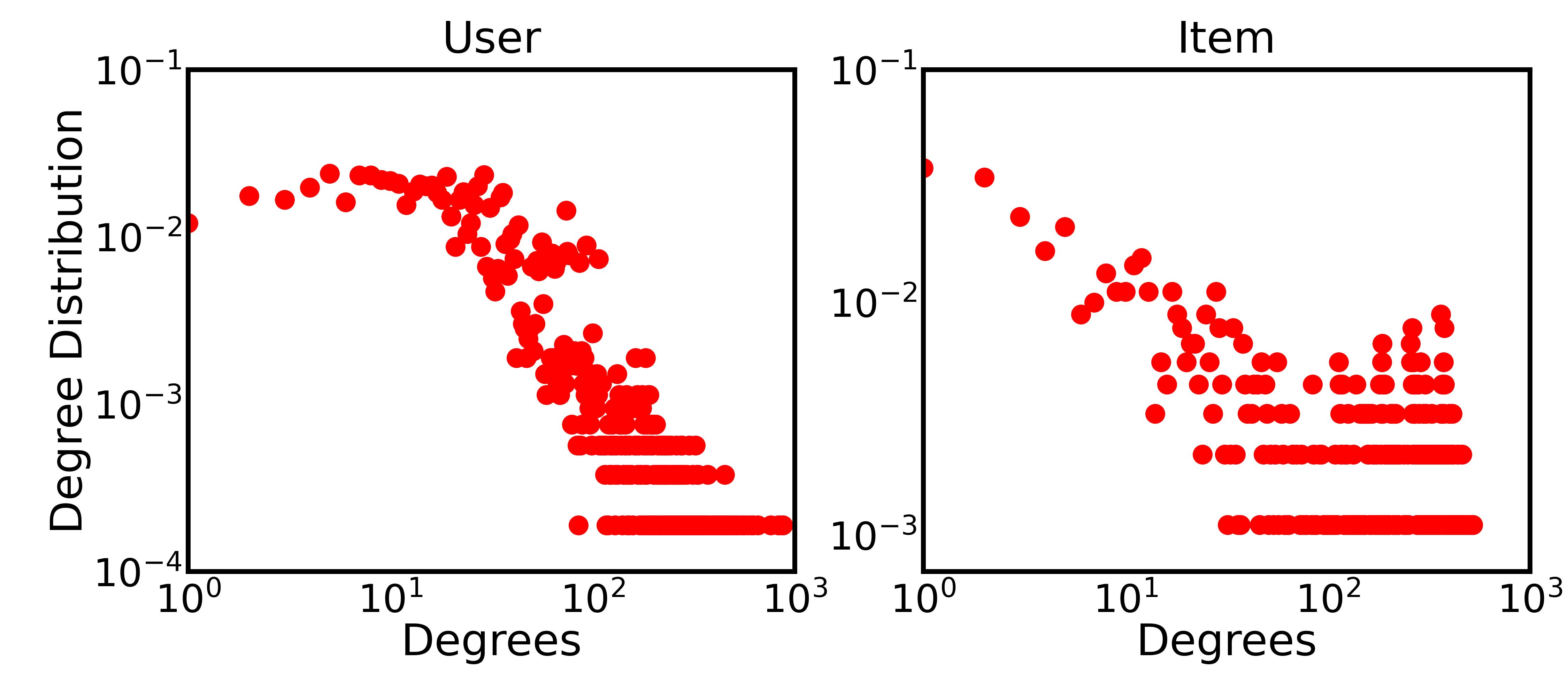
  Figure 1: User and item degree distribution on Wikipedia at the end interval.

• The second issue is on the network dynamics. We notice that Vinh Tran et al. [24], Yang et al. [4] represent sequential interaction networks on the hyperbolic manifolds very recently. They still assume the space is static same as the previous studies. The fact that the interaction network constantly evolves over time is largely ignored. It is also evidenced in the example in Fig. 1 and Table 1. Both $\delta$-hyperbolicity and degree distribution vary over time. In the language of Riemannian geometry, the previous studies attempt to learn user/item embeddings on a fixed curvature space, either Euclidean space or hyperbolic ones. Rather than a fixed curvature space, it calls for an evolving curvature space to manifest the inherent dynamics of the sequential interaction network, where the new interactions continuously arrive. The challenge lies in how to estimate curvature to model the space evolvement as it still lacks effective estimator in the literature.

In this paper, we argue that the representation space for sequential interaction network needs to model the difference between users and item (the first issue) and the evlovement over time (the second issue).

• The third issue is on the learning paradigm. The graph models is typically trained with abundant labels. Undoubtedly, the labels are expensive to acquire, and the reliability of the labels is sometimes questionable, especially for the case that the interactions continuously arrive. In the literature, the self-supervised learning on graphs without labels is roughly divided into generative methods and contrastive methods. The generative methods require a carefully designed decoder for data reconstruction. On the contrary, contrastive methods are free of decoder, and acquire knowledge by distinguishing the positive pairs from the negative pairs. Recently, contrastive learning has achieved the state-of-the-art performance for the typical graphs (e.g., social networks and citation networks), but it still remains open for sequential interaction networks.

Besides, most of the previous work [25, 26, 27, 28] consider that the interactions would only explicitly link the nodes of different type in the bipartite interaction graph while ignoring the implicit interaction among the same type of nodes. Indeed, it calls for new method to model such explicit and implicit impacts among the nodes.

To address the issues above, we propose a Contrastive Sequential Interaction Network learning model on Co-Evolving RiEmannian manifolds (CSincere). We first present a Co-evolving GNN to address the first and second issues. For the first issue, we propose to model the users and items in two different $\kappa$-stereographic spaces, i.e., Riemannian user space and Riemannian item space. The user space and item space are linked with the Euclidean tangent space, modeling the temporal interactions. Co-evolving GNN utilizes Cross-Space Aggregation for the message passing across different Riemannian spaces. For the second issue, we learn the temporal evolvement of user/item space curvatures via a neural curvature estimator (CurvNN). Co-evolving GNN utilizes CurvNN for both user and item spaces, so that they co-evolve with each other over time. Rather a single or static representation space, we for the first time embed the sequential interaction network into co-evolving Riemannian manifolds.

Our preliminary work above [29] has addressed the first and second issues, and this paper has equipped the original learning model on co-evolving Riemannian manifolds in [29] with a novel contrastive learning approach. Specifically, this full version further consider the issue of self-supervised learning for the sequential interaction network (i.e., the third issue). To this end, we introduce a Riemannian co-Contrastive learning for sequential interaction networks, where we propose to contrast between the temporal views generated in the evolvement. In the co-Contrastive learning, the novelty lies in that the users are co-contrasted with both users and items, and vice versa, so that Riemannian user space and Riemannian item space interact with each other. In the meanwhile, we pay more attention to both hard positive samples and hard negative samples with the reweighing mechanism. Finally, interacting between user space and item space, CSincere predicts future interactions without label information.

Overall, the noteworthy contributions of our work are summarized as follows:

• Problem. We rethink the bipartite nature, network dynamics and learning paradigm of sequential interaction network learning. It is the first attempt to introduce the co-evolving Riemannian manifolds, to the best of our knowledge.

• Model. We propose a novel co-evolving GNN with the cross-space aggregation, which represents the users and items in two different $\kappa$-stereographic spaces, co-evolving over time with the parameterized curvatures.

• Learning Paradigm. We propose a novel contrastive learning approach for sequential interaction networks, which interplays the co-evolving user and item space for interaction prediction.

• Experiment. Empirical results on 5 public datasets show the superiority of the proposed approach against the strong baselines.

Roadmap. The rest parts are organized as follows: We introduce the preliminary mathematics and formulate the studied problem in Sec. 2. To address this problem, we present the co-evolving graph neural network in Sec. 3, and the reweighted co-contrastive learning in Sec. 4. The empirical results of the proposed approach are reported in Sec. 5. We summarize the related work in Sec. 6, and finally conclude our work in Sec. 7.

2 Preliminaries & Problem Formulation

In this section, we first introduce the preliminary mathematics on Riemannian manifold and the notion of curvature. Then, we formulate the studied problem of self-supervised Riemannian sequential interaction network learning.

2.1 Riemannian Manifold

A smooth manifold $\mathcal{M}$ is said to be a Riemannian manifold if it is endowed with a Riemannian metric $g$. The Riemannian metric is characterized as the positive-definite inner product defined on $\mathcal{M}$’s tangent space $g_{\boldsymbol{x}}:\mathcal{T}_{\boldsymbol{x}}\mathcal{M}\times\mathcal{T}_{\boldsymbol{x}}\mathcal{M}\rightarrow\mathbb{R}$. Concretely, the tangent space $\mathcal{T}_{\boldsymbol{x}}\mathcal{M}$ is associated with a point $\boldsymbol{x}$ on the manifold, approximating the locality of the geometry with Euclidean space. That is, a Riemannian manifold is a tuple $(\mathcal{M},g)$ where $g_{\boldsymbol{x}}(\boldsymbol{v},\boldsymbol{v})\geq 0,g_{\boldsymbol{x}}(\boldsymbol{u},\boldsymbol{v})=g_{\boldsymbol{x}}(\boldsymbol{v},\boldsymbol{u})$ with $\boldsymbol{x}\in\mathcal{M}$ and $\boldsymbol{u},\boldsymbol{v}\in\mathcal{T}_{\boldsymbol{x}}\mathcal{M}$.

2.2 The $\kappa-$stereographic Model

In Riemannian geometry, there exists three kinds of isotropic spaces: hyperbolic, spherical and Euclidean space. Note that, the vectors in either the hyperbolic or the spherical space cannot be operated as the way we are familiar with in Euclidean space. The $\kappa$-stereographic model [22] unifies the vector operations of the aforementioned three kinds of isotropic spaces with gyrovector formalism [30]. (Notations: Bold lowercase $\boldsymbol{x}$ and bold uppercase $\boldsymbol{X}$ denote the vector and matrix, respectively.)

Without loss of generality, we consider the $n$-dimensional model ($n\geq 1$). The $\kappa$-stereographic model is a smooth manifold $\mathcal{M}_{\kappa}^{n}=\left\{\boldsymbol{x}\in\mathbb{R}^{n}\mid-\kappa\|\boldsymbol{x}\|_{2}^{2}<1\right\}$ equipped with a Riemannian metric $g_{\boldsymbol{x}}^{\kappa}=\left(\lambda_{\boldsymbol{x}}^{\kappa}\right)^{2}\boldsymbol{I}$, where $\kappa\in\mathbb{R}$ is the (sectional) curvature and $\lambda_{\boldsymbol{x}}^{\kappa}=2\left(1+\kappa\|\boldsymbol{x}\|_{2}^{2}\right)^{-1}$ is the conformal factor defined on the point $\boldsymbol{x}$. More specifically, when $\kappa>0$, $\kappa$-stereographic model shift to the spherical space (i.e., the stereographic projection of the hypersphere model. When $\kappa<0$, $\kappa$-stereographic model shift to the hyperbolic space (i.e., the Poincaré ball model with the radius of $1/\sqrt{-\kappa}$), and $\kappa$-stereographic model becomes Euclidean with $\kappa=0$ as a special case. Now, we introduce the gyrovector operations as follows.

Möbius Addition. In the gyrovector formalism, Möbius addition $\oplus_{\kappa}$ of two points $\boldsymbol{x},\boldsymbol{y}\in\mathcal{M}_{\kappa}^{n}$ is defined as follows:

$$\boldsymbol{x}\oplus_{\kappa}\boldsymbol{y} =\frac{\left(1-2\kappa\langle\boldsymbol{x},\boldsymbol{y}\rangle-\kappa\|\boldsymbol{y}\|_{2}^{2}\right)\boldsymbol{x}+\left(1+\kappa\|\boldsymbol{x}\|_{2}^{2}\right)\boldsymbol{y}}{1-2\kappa\langle\boldsymbol{x},\boldsymbol{y}\rangle+\kappa^{2}\|\boldsymbol{x}\|_{2}^{2}\|\boldsymbol{y}\|_{2}^{2}}.$$ (1)

Note that, the Möbius addition is non-associative.

Möbius Scaling and Matrix-Vector Multiplication. Scaling a $\kappa$-stereographic vector $\boldsymbol{x}\in\mathcal{M}_{\kappa}^{n}\backslash\left\{\boldsymbol{o}\right\}$ is defined with $\otimes_{\kappa}$ in Eq. (2), where $r\in\mathbb{R}$ is the scaling factor. The matrix-vector multiplication of any $\boldsymbol{M}\in\mathbb{R}^{m\times n}$ is given in Eq. (3) as follows:

$$r\otimes_{\kappa}\boldsymbol{x}= \frac{1}{\sqrt{\kappa}}\tan_{\kappa}\left(r\tan_{\kappa}^{-1}(\sqrt{\kappa}\|\boldsymbol{x}\|_{2})\right)\frac{\boldsymbol{x}}{\|\boldsymbol{x}\|_{2}},$$ (2)

$$\boldsymbol{M}\otimes_{\kappa}\boldsymbol{x}=(1/\sqrt{\kappa}) \tan_{\kappa}\left(\frac{\|\boldsymbol{M}\boldsymbol{x}\|_{2}}{\|\boldsymbol{x}\|_{2}}\tan_{\kappa}^{-1}(\sqrt{\kappa}\|\boldsymbol{x}\|_{2})\right)\frac{\boldsymbol{M}\boldsymbol{x}}{\|\boldsymbol{M}\boldsymbol{x}\|_{2}}.$$ (3)

Exponential and Logarithmic Maps. For any point $\boldsymbol{x}\in\mathcal{M}$, the bidirectional mapping between its living manifold $\mathcal{M}_{\kappa}^{n}$ and corresponding tangent space $\mathcal{T}_{\boldsymbol{x}}\mathcal{M}_{\kappa}^{n}$ is established by the exponential map $\exp_{\boldsymbol{x}}^{\kappa}:\mathcal{T}_{\boldsymbol{x}}\mathcal{M}_{\kappa}^{n}\rightarrow\mathcal{M}_{\kappa}^{n}$ and logarithmic map $\log_{\boldsymbol{x}}^{\kappa}:\mathcal{M}_{\kappa}^{n}\rightarrow\mathcal{T}_{\boldsymbol{x}}\mathcal{M}_{\kappa}^{n}$. The clean closed-form expression is given as follows:

$$\exp_{\boldsymbol{x}}^{\kappa}(\boldsymbol{v})=\boldsymbol{x}\oplus_{\kappa} \left(\tan_{\kappa}\left(\sqrt{|\kappa|}\frac{\lambda_{\boldsymbol{x}}^{\kappa}\|\boldsymbol{v}\|_{2}}{2}\right)\frac{\boldsymbol{v}}{\|\boldsymbol{v}\|_{2}}\right),$$ (4)

$$\log_{\boldsymbol{x}}^{\kappa}(\boldsymbol{y})=\frac{2}{\lambda_{\boldsymbol{x}}^{\kappa}\sqrt{|\kappa|}} \tan_{\kappa}^{-1}\left\|-\boldsymbol{x}\oplus_{\kappa}\boldsymbol{y}\right\|_{2}\frac{-\boldsymbol{x}\oplus_{\kappa}\boldsymbol{y}}{\left\|-\boldsymbol{x}\oplus_{k}\boldsymbol{y}\right\|_{2}}.$$ (5)

Distance Metric. In the $\kappa-$stereographic model, the distance $d_{\mathcal{M}}^{\kappa}\left(\cdot,\cdot\right)$ between two points $\boldsymbol{x},\boldsymbol{y}\in\mathcal{M}_{\kappa}^{n},\boldsymbol{x}\neq\boldsymbol{y}$ is defined as:

$$d_{\mathcal{M}}^{\kappa}\left(\boldsymbol{x},\boldsymbol{y}\right)=\frac{2}{\sqrt{|\kappa|}}\tan_{\kappa}^{-1}\left(\sqrt{|\kappa|}\left\|-\boldsymbol{x}\oplus_{k}\boldsymbol{y}\right\|_{2}\right).$$ (6)

In the gyrovector formalism, $\tan_{\kappa}(\cdot)=\tanh(\cdot)$ for $\kappa<0$, otherwise, $\tan_{\kappa}(\cdot)=\tan(\cdot)$.

2.3 Sectional Curvature and Ricci Curvature

In Riemannian geometry, the notion of curvature describes the extent how a curve deviates from being a straight line, or a surface deviates from being a plane. Specifically, sectional curvature and Ricci curvature are introduced to describe the global and local structure, respectively [31].

Sectional Curvature. For each point on the manifold, sectional curvature is defined by tracing over all two-dimensional subspaces passing through the point. It is a cleaner description compared to the Riemann curvature tensor [32]. Recent works [10, 33, 34] usually consider the case that sectional curvature is equal everywhere on the manifold, and thus the sectional curvatures are degraded as a single constant.

Ricci Curvature. Ricci curvature is defined by averaging sectional curvatures at a point. In the literature, there are several discrete variants of Ricci curvature defined for the graphs, e.g., Ollivier-Ricci curvature [35] and Forman-Ricci curvature [36]. The intuition of the Ricci curvature on graphs is to measure how the local geometry of an edge in the graph differs from a gird graph. Specifically, Ollivier version is a coarse approximation of Ricci curvature, while Forman version is combinatorial and faster to compute.

2.4 Problem Formulation

In this paper, we formally define a sequential interaction network as follows:

Definition (Sequential Interaction Network).

A sequential interaction network (SIN) is formulated a tuple $\mathcal{G}=\{\mathcal{U,I,E,T,X}\}$. $\mathcal{U}$ and $\mathcal{I}$ denote the user set and item set, respectively. Each user (item) is attached with a feature $\boldsymbol{u}\in\mathbb{R}^{d_{\mathcal{U}}}$ ($\boldsymbol{i}\in\mathbb{R}^{d_{\mathcal{I}}}$). $\mathcal{E}\subseteq\mathcal{U}\times\mathcal{I}\times\mathcal{T}$ is the interaction set. An interaction $e\in\mathcal{E}$ is defined as a triplet $e=(u,i,t)$, recording that user $u\in\mathcal{U}$ and item $i\in\mathcal{I}$ interact with each other at time point $t\in\mathcal{T}$. $\mathcal{X}\in\mathbb{R}^{|\mathcal{E}|\times d_{\mathcal{X}}}$ is the matrix summarizing the attributes of each interaction, where $d_{\mathcal{X}}$ is the dimensionality of the attributes.

Now, we define the problem of Self-supervised Representation Learning for Sequential Interaction Networks as follows:

Problem Definition.

For a sequential interaction network $\mathcal{G}$, it aims to learn encoding functions, mapping users/items to the representation space, which is able to model the difference between users and item (the first issue) and the evlovement over time (the second issue). Formally, we have $\Phi_{u}:\mathcal{U}\rightarrow\mathbb{U}_{\kappa_{u}}$ and $\Phi_{i}:\mathcal{I}\rightarrow\mathbb{I}_{\kappa_{i}}$, where $\mathbb{U}_{\kappa_{u}}$ and $\mathbb{I}_{\kappa_{i}}$ are two different Riemannian spaces modeling the structural patterns underlying the users and items, respectively. The curvatures $\kappa_{u}$ and $\kappa_{i}$ are the functions of time modeling the space evolvement over time. No label information is required (the first issue) to learn the encoding functions $\Phi_{u}$ and $\Phi_{i}$ so as to predict future interactions with user/item embeddings.

In short, we are interested in self-supervisedly representing the sequential interaction network on a couple of Riemannian user space and Riemannian item space, so that future interaction can be predicted with the user/item embeddings.

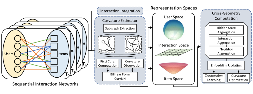
Figure 2: Illustration of Co-Evolving GNN. In practice, a sequence of interactions is divided into several batches according to the associated timestamps (denoted by different colors), and each batch is regarded as a time interval. Cross-Space Aggregation, Interaction Integration and the neural Curvature Estimator are elaborated in Sec. 3.1, Sec. 3.2 and Sec. 3.3, respectively. Accordingly, user/item embeddings and curvature are learned via the proposed contrastive learning approach and curvature optimization, respectively.

3 Co-Evolving Graph Neural Network

As shown in the examples and discussion in Sec. of Introduction, users and items present inherent difference, and the pattern evolves over time. Rather than a single and fixed-curvature representation space, we for the first time introduce the a couple of Riemannian manifolds whose curvature co-evolves over time, addressing the first and second issues. The novel representation space is referred to as co-evolving Riemannian manifolds, which is one of the core contribution of our work. Specifically, users and items are represented in the respective Riemannian manifolds, and the two manifolds are linked by a Euclidean tangent space, representing the interactions. The space evolvement over time is guided by a neural curvature estimator. The overall framework of Co-evolving GNN is presented in Fig. 2.

Before detailing Co-evolving GNN, we collect the main notations in Table 2. For the sake of clarity, we omit the subscript when no ambiguity will occur.

Table 2: Glossary of Main Notations in CSincere

Notation	Description
$\mathbb{U}_{\kappa_{u}}$	Riemannian user space associated with functional curvature $\kappa_{u}$ w.r.t. time
$\boldsymbol{u}_{j}(T)\in\mathbb{R}^{d_{U}}$	$d_{U}-$dimensional user embedding of user $j$ during $T$
$\mathbb{I}_{\kappa_{i}}$	Riemannian item space associated with functional curvature $\kappa_{i}$ w.r.t. time
$\boldsymbol{i}_{k}(T)\in\mathbb{R}^{d_{U}}$	$d_{I}-$dimensional item embedding of item $k$ during $T$
$T_{n}$	Time interval from $t_{n-1}$ to $t_{n}$
$\mathcal{N}_{u/i}^{T}$	The set of neighbors centered at user $u$ (item $i$) during $T$
$\kappa_{u/i}^{T}$	The value of (sectional) curvature of Riemannian user/item space during $T$
$\mathcal{E}_{u/i}^{T}$	The set of interactions linked to user $u$ (item $i$) during $T$

3.1 Cross-Space Aggregation for User and Item Modeling

In Co-evolving GNN, we propose to model the users and items in two different representation space: user space and item space. They are different Riemannian spaces of $\kappa$-stereographic model. User and item embeddings are collected in the matrices $\boldsymbol{U}$ and $\boldsymbol{I}$, respectively.

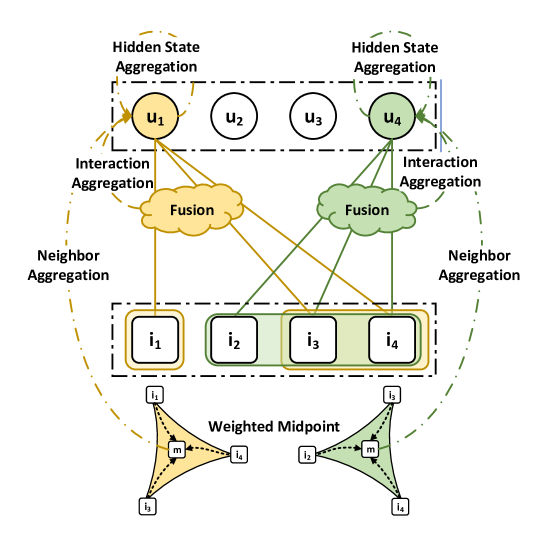
Figure 3: Illustration of Cross-Space Aggregation. We give an example of utilizing Eq. (7) to update user embedding once.

Typical message-passing in GNNs operates on a single representation space, either the classic Euclidean or the recent hyperbolic space. In contrast, message-passing operates on a couple of different Riemannian spaces in our design, but how to pass the message cross different spaces still largely remains open. To bridge this gap, we formulate the Cross-Space Aggregation with the gyrovector formalism. The formulation for user space and item space are given as follows,

$$\boldsymbol{u}_{j}(T_{n})\leftarrow\underbrace{\boldsymbol{M}_{1}\otimes_{\kappa_{u}^{T}}\boldsymbol{h}_{u_{j}}(T_{n})}_{\textit{user hidden aggregation}}\oplus_{\kappa_{u}^{T}}\underbrace{\boldsymbol{M}_{2}\otimes_{\kappa_{u}^{T}}\exp_{\boldsymbol{o}}^{\kappa_{u}^{T}}(\boldsymbol{e^{\prime}}_{u_{j}}^{T})}_{\textit{interaction aggregation}}\oplus_{\kappa_{u}^{T}}\underbrace{\boldsymbol{M}_{3}\otimes_{\kappa_{u}^{T}}\operatorname{map}_{\kappa_{i}^{T}}^{\kappa_{u}^{T}}(\boldsymbol{i^{\prime}}_{u_{j}}^{T})}_{\textit{item aggregation}},$$ (7)

$$\boldsymbol{i}_{k}(T_{n})\leftarrow\underbrace{\boldsymbol{M}_{4}\otimes_{\kappa_{i}^{T}}\boldsymbol{h}_{i_{k}}(T_{n})}_{\textit{item hidden aggregation}}\oplus_{\kappa_{i}^{T}}\underbrace{\boldsymbol{M}_{5}\otimes_{\kappa_{i}^{T}}\exp_{\boldsymbol{o}}^{\kappa_{i}^{T}}(\boldsymbol{e^{\prime}}_{i_{k}}^{T})}_{\textit{interaction aggregation}}\oplus_{\kappa_{i}^{T}}\underbrace{\boldsymbol{M}_{6}\otimes_{\kappa_{i}^{T}}\operatorname{map}_{\kappa_{u}^{T}}^{\kappa_{i}^{T}}(\boldsymbol{u^{\prime}}_{i_{k}}^{T})}_{\textit{user aggregation}},$$ (8)

where the matrices $\boldsymbol{M}$s are introduced for dimension transformation. The function $\operatorname{map}_{\kappa_{1}}^{\kappa_{2}}\left(\cdot\right)$ maps the vector living in the manifold of curvature $\kappa_{1}$ to the manifold of curvature $\kappa_{1}$ with the common reference (i.e., point of north pole of the $\kappa$-stereographic model). We provide a graphical illustration in Fig. 3 to show our idea. Next, we detail the component of Cross-Space Aggregation of Eq. (7) as follows:

• The first component updates the original hidden representation of user $j$.

• The second component aggregates the interactions associated with user $j$. Either Early Fusion or Late Fusion is acceptable for interaction aggregation, i.e., $\boldsymbol{e^{\prime}}_{u/i}^{T}=\textsc{Mlp}\left(\textsc{Pooling}\left(\boldsymbol{e}\in\mathcal{E}_{u/i}^{T}\right)\right)$ or $\boldsymbol{e^{\prime}}_{u/i}^{T}=\textsc{Pooling}\left(\textsc{Mlp}\left(\boldsymbol{e}\in\mathcal{E}_{u/i}^{T}\right)\right)$. The interaction modeling is introduced in the following subsection.

• The third component aggregates items information interacted with user $j$. Here, we utilize the well-defined weighted gyro-midpoints [37]. Concretely, the item aggregation surrounding user $u$ is formulated as

  $$\boldsymbol{i^{\prime}}_{u}^{T}=\textsc{Midpoint}_{\kappa_{i}^{T}}\left(x_{j}\in\mathcal{N}_{u}^{T}\right)=\frac{1}{2}\otimes_{\kappa_{i}^{T}}\left(\sum_{x_{j}\in\mathcal{N}_{u}^{T}}\frac{\alpha_{k}\lambda_{\boldsymbol{x}_{j}}^{\kappa}}{\sum_{x_{k}\in\mathcal{N}_{u}^{T}}\alpha_{k}\left(\lambda_{\boldsymbol{x}_{k}}^{\kappa}-1\right)}\boldsymbol{x}_{j}\right),$$ (9)

  where $\lambda_{\boldsymbol{x}}^{\kappa}$ is conformal factor introduced in Sec. 2.2. $\alpha_{k}$ is the weighting factor, and thus Eq. (9) is ready to incorporate with any off-the-shelf attention mechanism in $\kappa$-stereographic model.

Note that, the explicit interaction between the nodes of different types is captured in the Cross-Space Aggregation itself while the implicit interaction between the nodes of the same type is captured by stacking multiple layers, alleviating the issue of implicit interaction ignorance.

After the cross-space aggregation, we map user/item embeddings to next-period manifolds, and the updating rule is formulated as as follows:

$$\boldsymbol{u}_{j}(T_{n+1})=\operatorname{map}_{\kappa_{u}^{T_{n}}}^{\kappa_{u}^{T_{n+1}}}\left(\boldsymbol{u}_{j}\left(T_{n}\right)\right),$$ (10)

$$\boldsymbol{i}_{j}(T_{n+1})=\operatorname{map}_{\kappa_{i}^{T_{n}}}^{\kappa_{i}^{T_{n+1}}}\left(\boldsymbol{i}_{j}\left(T_{n}\right)\right),$$ (11)

where $\kappa^{T_{n+1}}$ is the next interval curvature obtained via Eq. 16.

3.2 Temporal Interaction Integration

Users and items are placed in different spaces, but they are presented as a whole with the temporal interactions. Thus, we utilize the common tangent space of the two Riemannian manifolds to model the interactions. In other words, user space and item space are linked by a Euclidean space, the the common tangent space.

Specifically, we first perform time encoding to encode the temporal information in the timestamps. In other words, we are interested in a function of time encoder $\Phi_{t}:\mathcal{T}\rightarrow\mathbb{R}^{d}$ that encodes a time point $t_{k}\in\mathcal{T}$ to a $d$-dimensional vector $\phi(t)\in\mathcal{T}$ in Euclidean space. We employ the well-defined harmonic encoder [38] formulated as follows:

$$\phi(t)=\sqrt{\frac{1}{d}}\left[\cos\left(\omega_{1}t+\theta_{1}\right),\cos\left(\omega_{2}t+\theta_{2}\right),\cdots,\cos\left(\omega_{d}t+\theta_{d}\right)\right],$$ (12)

where $\omega$ and $\theta$ are the learnable parameters to construct the time encoding. Then, for each interaction $e_{k}\in\mathcal{E}$, we perform Interaction Integration which integrates the timestamp and attribute with the following formulation,

$$\boldsymbol{e}_{k}=\sigma(\boldsymbol{W}_{7}\cdot\left[\boldsymbol{X}_{k}\ :\ \phi(t_{k})\right]),$$ (13)

where $\phi(t_{k})$ is the time encoding of the timestamp. $\left[\cdot:\cdot\right]$ denotes the concatenation. $\sigma(\cdot)$ denotes the nonlinearity and $\boldsymbol{W}_{7}$ is the parameter.

3.3 Curvature Estimator

The previous works in the literature model sequential interaction networks in a fixed curvature space, either zero or a negative constant. However, the fact is that the network as well as its underlying structural pattern evolves over time. In Riemannian geometry, structural pattern of a graph is characterized as curvature. That is, it is required to estimate the curvature to model the space evolvement over time.

In graph domain, the discrete curvatures such as Ricci curvature are introduced on the graph where the nodes are directly connected by the links (e.g., citation networks and social network). However, SIN is a different case that the users or the items are not directly connected, i.e., SIN is bipartite. We propose to bridge this gap by extracting a subgraph among the nodes of the same type. The rule is that two users (items) are linked to each other if they are interacted with $K$ same item (user). We further take sampling to accelerate the extraction process in practice.

We start with the definition of Ricci curvature $\kappa_{r}(x,y)$ to estimate curvature. Concretely, for any edge $(x,y)$, its Ricci curvature of Ollivier version [35] is defined as

$$\kappa_{r}(x,y)=1-\frac{W\left(m_{x},m_{y}\right)}{d_{\mathcal{M}}^{\kappa}(x,y)},$$ (14)

where $W(\cdot,\cdot)$ is Wasserstein distance between two mass distributions. For node $x$, we have $m_{x}^{\alpha}\left(x_{i}\right)$, the mass distribution defined over its one-hop neighboring nodes $\mathcal{N}(x)=\{x_{1},x_{2},...,x_{l}\}$.

$$m_{x}^{\alpha}\left(x_{i}\right)=\begin{cases}\alpha&\text{ if }x_{i}=x,\\ (1-\alpha)/l&\text{ if }x_{i}\in\mathcal{N}(x),\\ 0&\text{ otherwise. }\end{cases}$$ (15)

where we have $\alpha=0.5$ following the previous works [31, 39]. We collect Ricci curvatures of a time interval in the vector $\boldsymbol{r}$. According to the bilinear relationship between Ricci curvature and sectional curvature, we design a neural curvature estimator, referred to as CurvNN, to estimate the global curvature as follows,

$$\kappa_{e}=MLP\left(\boldsymbol{r}\right)^{\top}\boldsymbol{W}_{8}MLP\left(\boldsymbol{r}\right),$$ (16)

where $MLP$ is short for Multi-Layer Perceptron and $\boldsymbol{W}_{8}$ is a parameter. Note that, the formulation in Eq. (16) is able to learn the curvature of any sign without loss of generality.

Input : An undirected graph $G$, iterations $n$

Output : Observed curvature $\kappa_{o}$

1 for $m\in G$ do

2       for $i=1,...,n$ do

3             $b,c\in\mathop{Sample}(\mathcal{N}(m))$ and $a\in\mathop{Sample}(G)/\{m\}$;

4             Calculate $\gamma_{\mathcal{M}}(a,b,c)$;

5             Calculate $\gamma_{\mathcal{M}}(m;b,c;a)$;

6            

7      Let $\gamma(m)=\mathop{MEAN}(\gamma_{\mathcal{M}}(m;b,c;a))$;

8      

Return: $\kappa_{o}=\mathop{MEAN}(\gamma(m))$

Algorithm 1 Observed Curvature

Meanwhile, we utilize the observation of the curvature to learn CurvNN. Concretely, we leverage the Parallelogram Law in Riemannian space [40, 41, 22] to observe the sectional curvature. With a geodesic triangle $abc$ on the manifold, we have the equations below,

$$\gamma_{\mathcal{M}}(a,b,c)= d_{\mathcal{M}}(a,m)^{2}+\frac{d_{\mathcal{M}}(b,c)^{2}}{4}-\frac{d_{\mathcal{M}}(a,b)^{2}+d_{\mathcal{M}}(a,c)^{2}}{2},$$ (17)

$$\gamma_{\mathcal{M}}(m;b,c;a)= \frac{\gamma_{\mathcal{M}}(a,b,c)}{2d_{\mathcal{M}}(a,m)},$$

where $m$ is the midpoint of $bc$. Eq. (17) describes the extent how a triangle in the manifold deviates from being a normal triangle in Euclidean space. Recall that the notion of curvature describes the extent how a surface deviates from being a plane, and Eq. (17) is an intuitive analogy to the triangles. Accordingly, the observed curvature $\kappa_{o}$ is figured out by Algorithm 1, providing the supervision for CurvNN. Then, the loss of curvature optimization is given as $\mathcal{J}_{c}=|\kappa_{e}-\kappa_{o}|^{2}$ so as to maximize the agreement between the estimated curvature and the observations.

4 Riemannian Co-Contrastive Learning

In this section, we present the co-contrastive learning for sequential interaction network on the Riemannian manifolds. The novelty lies in that, in the co-contrast, user space and item space interact with each other for interaction prediction. In the meantime, we pay more attention to both hard negative and hard positive samples with the reweighing mechanism on Riemannian manifolds.

4.1 Co-Contrast Strategy

Contrastive learning acquires knowledge without external guidance (labels) via exploring the similarity from the data itself, and has achieved great success in graph learning tasks [42, 43, 44]. Recently, [45, 46] make effort on the contrastive learning for temporal networks. However, they are inherently different from the sequential interaction network, where the disjoint user and item set are linked by temporal interactions. Thereby, typical contrast strategy leads to inferior performance. Concretely, contrasting the users (items) with themselves regardless of the other set tends to destroy the correlation of users and items in SIN as a whole.

To bridge this gap, we introduce a co-contrast strategy, contrasting the users (items) with themselves as well as their counterparts simultaneously. For each anchor $x$, contrastive learning learns informative embeddings by distinguishing the positive samples ($x^{+}$) of $x$ from the negative ones ($x^{-}$) in the augmented view. In the co-contrast strategy, we first self-augment the graph leveraging the temporal evolvement, and create different temporal views. We take the user space for the illustration and give a toy example in Fig. 4. At time $t_{2}$, user embeddings derived from our model term as the $\alpha$ view (denoted as $u^{\alpha}$). Those mapped from the history embedding at $t_{1}$ via mapping $\Gamma$ term as the $\beta$ view (denoted as $u^{\beta}$). The mapping is given as

$$\Gamma(\cdot)=map^{\kappa_{U}(t_{2})}_{\kappa_{U}(t_{1})}(\cdot,).$$ (18)

Second, we derive the image of the counterpart space for the co-contrast. In Fig. 4, given the anchor $u_{4}$, we co-contrast $u_{4}^{\alpha}$ with the users and item’s images in $\beta$ view. The negative samples are all $u^{\beta}_{j}(j\neq 4)$, while the positive samples ($u_{k}^{+}$) are $u_{4}^{\beta}$ and the images of $i_{k}^{\beta}$ ($i_{k}$ are the items linking to $u_{4}$ at $t_{2}$). The item’s image is given as $map^{\kappa_{U}(t_{2})}_{\kappa_{I}(t_{2})}(\cdot)$.

The advantage of the proposed strategy is that, in the co-contrast, the user space interacts with the item space and vice versa, so as to capture user-item correlation and facilitate interaction prediction.

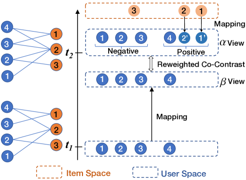
Figure 4: A toy example of the co-contrast strategy.

4.2 Temporal Similarity on Riemannian Manifolds

Measuring similarity in the sequential interaction network is nontrivial. On the one hand, Euclidean functions cannot be used on the Riemannian Manifolds. On the other hand, typical similarity function is time-independent [47, 48, 43] but temporal information is important for sequential interaction networks. To this end, we formulate a temporal similarity function on Riemannian manifolds as follows,

$$sim(x_{1},x_{2})=(\boldsymbol{t}_{1}^{T}\boldsymbol{t}_{2})\operatorname{Sigmoid}\left(-d(\boldsymbol{x}_{1},\boldsymbol{x}_{2})\right),$$ (19)

where $d(\cdot,\cdot)$ is the distance function on Riemannian manifolds, and $\boldsymbol{t}_{i}$ is the time encoding of $t_{i}$ derived via $\boldsymbol{t}_{i}=\phi(t_{i})$ in Eq. (12).

We show that the inner product term in Eq. (19) is a function of the time span $(t_{2}-t_{1})$, encoding the relative pattern between the samples with respect to the time (i.e., translation invariant).

We start with the Bochner’s Theorem as follows.

Bochner’s Theorem.

A translation-invariant kernel $\mathcal{K}(x,y)=f(x-y)$ is positive definite, where $\mathcal{K}$ is continuous and is defined on $\mathbb{R}^{d}$, if and only if there exists a non-negative measure on $\mathbb{R}$ such that $f$ is the Fourier transformation of the measure.

Now, we prove the translation invariant of the inner product (Proposition 1).

Proposition 1 (Translation Invariant).

Given the time encoding in Eq. (12), there exists a real function $f$ such that the inner product of time encoding at $t_{2}$ and $t_{1}$ can be expressed as $f(t_{2}-t_{1})$.

Proof.

According to the Bochner’s Theorem, the proposition holds if the kernel $\mathcal{K}$ induced by the time encoding in Eq. (12) is translation invariant. Given the fact of trigonometric functions, induced kernel $\mathcal{K}$ is given as

$$\mathcal{K}(t_{1},t_{2})=\phi(t_{1})^{\top}\phi(t_{1}) =\mathbb{E}_{\omega}\left[\cos\left(\omega t_{1}\right)\cos\left(\omega t_{2}\right)+\sin\left(\omega t_{1}\right)\sin\left(\omega t_{2}\right)\right]$$ (20)

$$=\mathbb{E}_{\omega}\left[\cos\left(\omega\left(t_{1}-t_{2}\right)\right)\right],$$

where $\omega$ is specified in Eq. (12). With a non-negative probability measure $p(\omega)$ on $\mathbb{R}$, we consider the Fourier transformation as follows,

$$\mathbb{E}_{\omega}\left[\xi_{\omega}\left(t_{1}\right)\xi_{\omega}\left(t_{2}\right)^{*}\right]=\int_{\mathbb{R}}e^{i\omega\left(t_{1}-t_{2}\right)}p(\omega)d\omega=f(t_{1}-t_{2}),$$ (21)

where $\xi_{\omega}(t)=e^{i\omega t}$. $i$ is the image unit, and $*$ denotes the complex conjugate. Eq. (20) is the real part of the Fourier transformation, and there exists a real $f$ when scaled properly [38]. That is, the kernel $\mathcal{K}$ is translation invariant, and thereby $\mathcal{K}(t_{1},t_{2})=f(t_{2}-t_{1})$. ∎

Remark. Note that, $f$ is learned in the contrastive learning, and additionally, the $f$ implied in Eq. (19) has better expressive ability than the exponential decay, as shown in the Ablation Study in Sec. 5.

4.3 Reweighing InfoNCE Loss

The classic InfoNCE with a standard binary cross-entropy [46, 48] is given as follows,

$$-\mathbb{E}_{x}\left[\mathbb{E}_{x^{+}\sim p^{+}}log\frac{1}{1+e^{-sim(x,x^{+})}}+\mathbb{E}_{x^{-}\sim p^{-}}log\frac{1}{1+e^{sim(x,x^{-})}}\right],$$ (22)

A major shortcoming of the InfoNCE loss above is that all the samples in the augmented view are treated equally, i.e., neglecting the hardness of the samples [49, 50]. However, the importance of different samples tends to be different in the contrastive learning. More attention to the hard samples boosts the learning performances. A hard negative has a similar representation to the anchor so that it is hard to be distinguished. Similarly, in the case of positive pairs, more attention is required when the positive sample is far away from the anchor in the representation space, which is known as hard positive. Accordingly, we suggest the following sampling distribution for negative and positive samples,

$$q^{-}_{\eta}\propto e^{\eta sim(x,x^{-})}p^{-},\quad q^{+}_{\eta}\propto e^{-\eta sim(x,x^{+})}p^{+}.$$ (23)

Note that, the nonnegative $\eta$ controls the impact of hard samples, and we have $\eta=2$ in practice. $sim(\cdot,\cdot)$ is the similarity measure on the Riemannian manifolds. Concretely, we introduce a normalizing constant to ensure the mass of the distribution equals to $1$, e.g., $q^{-}_{\eta}(x^{-})=\frac{1}{Z^{-}}e^{\eta sim(x,x^{-})}p^{-}(x^{-})$.

Hence, we derive the Reweighed InfoNCE Loss with the distributions in Eq. (23) as follows,

$$-\mathbb{E}_{x}\left[\mathbb{E}_{x^{+}\sim q_{\eta}^{+}}\log\frac{1}{1+e^{-sim(x,x^{+})}}+\mathbb{E}_{x^{-}\sim q_{\eta}^{-}}\log\frac{1}{1+e^{sim(x,x^{-})}}\right].$$ (24)

Equivalently, we rewrite Eq. (24) with the original distributions as

$$\mathbb{E}_{x^{+}\sim q_{\eta}^{+}}\log\frac{1}{1+e^{-sim(x,x^{+})}}=\mathbb{E}_{x^{+}\sim p^{+}}\left[\frac{q_{\eta}^{+}}{p^{+}}\log\frac{1}{1+e^{-sim(x,x^{+})}}\right],$$ (25)

$$\mathbb{E}_{x^{-}\sim q_{\eta}^{-}}\log\frac{1}{1+e^{sim(x,x^{-})}}=\mathbb{E}_{x^{-}\sim p^{-}}\left[\frac{q_{\eta}^{-}}{p^{-}}\log\frac{1}{1+e^{sim(x,x^{-})}}\right].$$ (26)

The intuition of the proposed loss is that we up-weight the hard samples in the contrastive learning, as shown in the right hand side of equation above.

4.4 Reweighed Co-Contrast Loss

For the user space, we formulate the reweighed co-contrast loss as follows,

$$\mathcal{J}^{U}_{(\alpha,\beta)}=-\frac{1}{|\mathcal{U}|}\sum_{i=1}^{|\mathcal{U}|}\left(\mathcal{J}^{+}(\boldsymbol{u}_{i}^{\alpha},\boldsymbol{u}_{k}^{\beta})+\mathcal{J}^{-}(\boldsymbol{u}_{i}^{\alpha},\boldsymbol{u}_{j}^{\beta})\right),$$ (27)

where

$$\mathcal{J}^{+}(\boldsymbol{u}_{i}^{\alpha},\boldsymbol{u}_{k}^{\beta})=\sum_{k=1}^{K^{+}}\frac{e^{-\eta sim(\boldsymbol{u}_{i}^{\alpha},\boldsymbol{u}_{k}^{\beta})}}{Z^{+}}\log\frac{1}{1+e^{-sim(\boldsymbol{u}_{i}^{\alpha},\boldsymbol{u}_{k}^{\beta})}},$$ (28)

$$\mathcal{J}^{-}(\boldsymbol{u}_{i}^{\alpha},\boldsymbol{u}_{j}^{\beta})=\sum_{j=1}^{K^{-}}\frac{e^{\eta sim(\boldsymbol{u}_{i}^{\alpha},\boldsymbol{u}_{j}^{\beta})}}{Z^{-}}\log\frac{1}{1+e^{sim(\boldsymbol{u}_{i}^{\alpha},\boldsymbol{u}_{j}^{\beta})}}.$$ (29)

$K^{+}$ and $K^{-}$ are the number of positive samples and negative samples, respectively. $\{\boldsymbol{u}_{j}\}_{j\neq i}$ is the set of negative samples. The positive sample set $\{\boldsymbol{u}_{k}\}$ consists of $\boldsymbol{u}_{i}$ and the images of items linking to $\boldsymbol{u}_{i}$. That is, we co-contrast users with themselves and the correlated items simultaneously. The normalizing constants are given as

$$Z^{+}=\frac{1}{K^{+}}\sum_{k=1}^{K^{+}}e^{-\eta sim(\boldsymbol{u}_{i}^{\alpha},\boldsymbol{u}_{k}^{\beta})},\quad Z^{-}=\frac{1}{K^{-}}\sum_{j=1}^{K^{-}}e^{\eta sim(\boldsymbol{u}_{i}^{\alpha},\boldsymbol{u}_{j}^{\beta})}.$$ (30)

With the formulation above, it is obvious that the samples are reweighed by a softmax-like coefficient so that hard samples are regulated by the learnt importance. Different from the previous reweighing mechanism [46, 50, 45], the proposed reweighing not only regulates the hard samples in the user space iteslf, but also regulates the hard samples in the counterpart space.

Similarly, the reweighed co-contrastive loss for the items is given as follows,

$$\mathcal{J}^{I}_{(\alpha,\beta)}=-\frac{1}{|\mathcal{I}|}\sum_{i=1}^{|\mathcal{I}|}\left(\mathcal{J}^{+}(\boldsymbol{i}_{i}^{\alpha},\boldsymbol{i}_{k}^{\beta})+\mathcal{J}^{-}(\boldsymbol{i}_{i}^{\alpha},\boldsymbol{i}_{j}^{\beta})\right).$$ (31)

Input : A sequential interaction network $\mathcal{G}=\{\mathcal{U,I,E,T,X}\}$

Output : 1) User and item embeddings $\boldsymbol{U}$,$\boldsymbol{I}$

2) A well-trained CurvNN

1 Initialize user/item embeddings $\boldsymbol{u}_{j}$, $\boldsymbol{i}_{k}$ and map them to the respective manifold via Eq. 4;

2 Initialize time encoding for interaction embeddings $\boldsymbol{e}$ via Eq. 13;

3 for $epoch=1,...,N$ do

4       for  each $batch=t$ do

5             Feed Ricci curvatures into CurvNN via Eq. 16;

6             Calculate the observed curvature via Algorithm 1;

7             Generate the $\alpha$ view by forwarding Co-evolving GNN in Eq. (7-11);

8             Generate the $\beta$ view by mapping from the history embeddings via Eq. (18);

9             Calculate the Reweighed Co-Contrast loss in Eq. (27-31);

10             Calculate the overall loss in Eq. (32);

11             Back propagation, update parameters;

12             Record the curvature of batch $t$;

13            

14      

Algorithm 2 Self-supervised Learning

Overall Loss of CSincere. Finally, we formulate the overall loss of CSincere below,

$$\mathcal{L}=\left(\mathcal{J}^{U}_{(\alpha,\beta)}+\mathcal{J}^{U}_{(\beta,\alpha)}\right)+w_{1}\left(\mathcal{J}^{I}_{(\alpha,\beta)}+\mathcal{J}^{I}_{(\beta,\alpha)}\right)+w_{2}\mathcal{J}_{c},$$ (32)

where the $\alpha$ view is contrasted with the $\beta$ view, and vice versa. $\mathcal{J}_{c}$ is the loss of curvature optimization in Sec. 3.3, and the $w$’s are weighting coefficients.

In summary, CSincere learns user and item embeddings on co-evolving Riemannian manifolds, where user space and item space interact with each other in the (Reweighed) Co-Contrastive Learning for interaction prediction.

4.5 Computational Complexity Analysis

The procedure to train our CSincere is summarized in Algorithm 2. The most expensive component of our model is the Reweighed Co-Contrast, whose computational complexity is $O(|\mathcal{U}|(|\mathcal{U}|+D_{U})+|\mathcal{I}|(|\mathcal{I}|+D_{I}))$. Concretely, the former term is the complexity of the contrastive learning in the user space, and $D_{U}$ is the user’s maximum degree. The degree here means the number of items linking to the user. The latter one is the complexity of the contrastive learning in the item space, and $D_{I}$ is the item’s maximum degree. In the curvature estimation, the most expensive component is to solve the Wasserstein distance sub-problem implied in the Olliver-Ricci curvature. The computational complexity is $O(V^{3}\log V)$, where $V$ is the number of the nodes in the subgraph introduced in Sec 3.3. It is noteworthy to mention that the Olliver-Ricci curvature can be effectively obtained following [51, 52]. In addition, to avoid repeated calculation of Olliver-Ricci curvature, we adopt an Offline computation and saves it in advance as a pre-processing for each batch.

5 Experiments

In this section, we compare the proposed CSincere with $10$ strong baselines on $5$ public datasets with the aim of answering the research questions as follows (RQs):

• RQ1: How does the proposed CSincere perform?

• RQ2: How does the proposed component contributes to the success of CSincere?

• RQ3: How is CSincere sensitive to the hyperparameters?

5.1 Experiment Setups

5.1.1 Datasets

To examine the performance of CSincere, we conduct experiments on $\boldsymbol{5}$ real-world datasets: MOOC, Wikipedia, Reddit, LastFM and Movielen [25, 5, 26]. The statistics of the datasets are detailed in Table 3.

Table 3: Statistics of datasets

Dataset	#Users	#Items	#Links	#Features
MOOC	7,047	97	411,749	4
Wikipedia	8,227	1,000	157,474	172
Reddit	10,000	984	672,447	172
LastFM	980	1000	1,293,103	0
Movielen	610	9,725	100,836	300

5.1.2 Baselines

To evaluate the effectiveness of our model, we compare our model with $\boldsymbol{10}$ state-of-the-art baselines, which are categorized as follows:

• Recurrent models: We compare with a family of RNNs designed for sequence data: LSTM, T-LSTM [27], RRN [53].

• Random walking models: CAW [5], CTDNE [18] are two temporal network models. The former adopts causal and anonymous random walks.

• Interaction models: JODIE [25], HILI [26] and DeePRed [19] are three state-of-the-art methods employing recursive network to model the user-item interaction.

• Hyperbolic models: HGCF [54] is a hyperbolic method on collaborative filtering.

Note that, none of the existing studies consider SIN learning on the generic Riemannian manifolds, to the best of knowledge. We the first time bridge this gap to learn SIN on the co-evolving Riemannian manifolds. Also, we include the conference version Sincere [29] as a baseline, and present the detailed comparison between the proposed model and Sincere in Sec. 5.2.

5.1.3 Evaluation Metrics

In this paper, we employ two metrics, Mean Reciprocal Rank ($MRR$) and $Recall@k$ to measure the performance of all methods.

• $Recall@k$ is defined as $=\frac{1}{N}\sum\nolimits_{i=1}^{N}\mathbb{I}(rank_{i}<=k)$, where $\mathbb{I}(\cdot)$ is the indicator function. $Recall@k$ means the true items appear in the top $k$ of sorted relevant item candidates.

• $MRR$ is defined as $\frac{1}{N}\sum\nolimits_{i=1}^{N}{\frac{1}{{rank_{i}}}}$, where $rank_{i}$ is the rank of predicted $i$-th item, and $N$ is the amount of all items. Accordingly, $MRR$ highlights the ranking of the prediction, and performs better than mean rank due to its stability.

The higher the metrics, the better the performance.

5.1.4 Implementation Details

The baselines are implemented with settings of the best performance according to the original papers. We conduct the $80\%-10\%-10\%$ train-valid-test split with the chronological order of the interaction samples If user/item feature are Euclidean, we map the features to respective Riemannian space via the logarithmic map. In CSincere, we have $w_{1}=1$ to balance the contrast between user space and item space. $w_{2}=10$ so as to highlight the curvature learning. $\eta=2$ in order to highlight the hard samples in the reweighting mechanism in our co-contrast approach. The embedding dimension is set to $64$ as default. Given the parameters live in the Euclidean tangent space with our design, CSincere is optimized at ease, and the Adam optimizer is employed where the learning rate is $0.001$ while the dropout rate is $0.3$. For the Riemannian baselines (i.e., HGCF, Sincere and CSincere), we set set the embedding dimension as $64$ to ensure a fair comparison. In practice, with the current batch of interactions, we first estimate the curvatures of the next batch via CurNN, and then infer the probability of the items interacting with the target user. A ranked list of top-$k$ items is given for interaction prediction.

Table 4: Future interaction prediction: Performance comparison in terms of mean reciprocal rank ($MRR$) and $Recall@10$. The best results are in bold and second best results are underlined.

	MOOC		Wikipedia		Reddit		LastFM		Movielen
Method	$MRR$	$Recall$	$MRR$	$Recall$	$MRR$	$Recall$	$MRR$	$Recall$	$MRR$	$Recall$
LSTM	0.055	0.109	0.329	0.455	0.355	0.551	0.062	0.119	0.031	0.060
T-LSTM	0.079	0.161	0.247	0.342	0.387	0.573	0.068	0.137	0.046	0.084
RRN	0.127	0.230	0.522	0.617	0.603	0.747	0.089	0.182	0.072	0.181
CAW	0.200	0.427	0.656	0.862	0.672	0.794	0.121	0.272	0.096	0.243
CTDNE	0.173	0.368	0.035	0.056	0.165	0.257	0.010	0.011	0.033	0.051
JODIE	0.465	0.765	0.746	0.822	0.726	0.852	0.195	0.307	0.428	0.685
HILI	0.436	0.826	0.761	0.853	0.735	0.868	0.252	0.427	0.469	0.784
DeePRed	0.458	0.532	0.885	0.889	0.828	0.833	0.393	0.416	0.441	0.472
HGCF	0.284	0.618	0.123	0.344	0.239	0.483	0.040	0.083	0.108	0.260
Sincere	0.586	0.885	0.793	0.865	0.825	0.883	0.425	0.466	0.511	0.819
CSincere	0.630	0.912	0.859	0.908	0.867	0.931	0.478	0.526	0.554	0.831

5.2 RQ1: Future Interaction Prediction

The task of interaction prediction is to predict the next item that a user will interact with historical iterations

We summarize the prediction results on all the datasets in terms of both $MRR$ and $Recall@10$ in Table 4. Note that, we report the empirical results of the mean value of $5$ independent run for fair comparison. As shown in Table 4, our CSincere achieves the best results in most of the cases. It shows the effectiveness of our idea, introducing the co-evolving Riemannian manifolds to learn the sequential interaction network. In the experiments, first, we find that the performance of the state-of-the-art JODIE and HILI has a relatively strong reliance on the time-independent component of the embeddings. We have reported such finding in the conference version [29], and in this paper, we focus on the proposed contrastive model. Second, among all methods, we find that CSincere, Sincere as well as DeePRed present high $MRR$ and $Recall@10$ with the smallest gaps. It shows that these models can not only make good prediction but also distinguish the groundtruth item from negative ones with higher ranks.

Comparing SINCERE. Here, we discuss on the methodology, computational complexity and, more importantly, the effectiveness. Both the proposed model and the previous SINCERE consider the representation learning on co-evolving Riemannian manifolds and build with the co-evolving GNN. The difference lies in the learning paradigm. SINCERE conducts the generative learning that reconstructs the temporal interactions in chronological order, while our model leverages the novel co-contrastive learning. In terms of computational complexity, SINCERE is in the order of $O(|\mathcal{E}|)$, where $|\mathcal{E}|$ is the number of interactions. Our model is in the order of $O(N^{2})$, $N=max(|\mathcal{U}|,|\mathcal{I}|)$. The complexity of our model is slightly higher than that of SINCERE as $\mathcal{E}\subseteq\mathcal{U}\times\mathcal{I}\times\mathcal{T}$, and is in the same order as typical contrastive graph model such as [43, 44, 48]. In terms of effectiveness, it is noteworthy to mention that our model consistently outperforms SINCERE, showing the superiority of the reweighted co-contrastive learning. We further investigate our contrastive learning approach in the following section.

Table 5: Ablation study on Wikipedia and Movielen datasets.

		Wikipedia		Movielen
Variant		$MRR$	$Recall@10$	$MRR$	$Recall@10$
Zero	Sincere	0.692	0.758	0.374	0.616
	$w/oKernel$	0.717	0.806	0.442	0.718
	$w/oReweigh$	0.743	0.822	0.439	0.692
	$w/oCoCon$	0.671	0.747	0.352	0.605
	CSincere	0.786	0.835	0.461	0.733
Static	Sincere	0.747	0.834	0.402	0.664
	$w/oKernel$	0.782	0.867	0.515	0.789
	$w/oReweigh$	0.779	0.849	0.483	0.756
	$w/oCoCon$	0.705	0.852	0.410	0.713
	CSincere	0.818	0.894	0.527	0.802
Evolve	Sincere	0.793	0.865	0.511	0.819
	$w/oKernel$	0.812	0.893	0.536	0.822
	$w/oReweigh$	0.808	0.871	0.529	0.827
	$w/oCoCon$	0.762	0.859	0.497	0.810
	CSincere	0.859	0.908	0.554	0.831

5.3 RQ2: Ablation Study

In this section, we study how the proposed component contributes to the success of CSincere. To this end, we introduce 6 kinds of variants as follows:

• To evaluate the effectiveness of Riemannian manifold (i.e., $\kappa$-stereographic spaces), we introduce the Euclidean variant by fixing the curvature to zero, denoted as $Zero$.

• To evaluate the effectiveness of curvature evolvement via $CurvNN$, we introduce the static variant denoted as $Static$. The curvature is estimated over the entire network regardless of time information.

• To evaluate the effectiveness of similarity based on transition invariant kernel, we introduce the variant by replacing the inner product in Eq. (19) with an exponential decay, denoted as $w/oKernel$.

• To evaluate the effectiveness of Reweighing, we introduce the variant disabling the reweighing mechanism, denoted as $w/oReweigh$. That is, we utilize the InfoNCE loss on Riemannian manifolds.

• To evaluate the effectiveness of Co-Contrast, we introduce the variant that separately contrast each space with itself regardless of the other, denoted as $w/oCoCon$. Concretely, we remove the positive samples of the counterpart space.

• We include the previous version of our model (ConfVer) as a reference in the discussion.

We report their performance on Wikipedia and Movielen datasets in Table 5, and find that: 1) The models with evolving curvatures consistently outperform the models of zero and static curvatures. It shows that the proposed $CurvNN$ effectively captures the structural evolvement over time. Rather than Euclidean space or a static curvature space, the proposed co-evolving Riemannian manifold is well aligned with the sequential interaction network, inherently explaining the superiority of our model and the inferiority of the baselines. 2) CSincere beats those $w/oKernel$. It shows the better expressive ability of the proposed kernel than that of the exponential decay. 3) CSincere has better results than those $w/oReweigh$. It suggests the necessity of paying more attention to the hard samples and the effectiveness of our reweighing. 4) CSincere has better results than those $w/oCoCon$. Also, we observe that $w/oCoCon$ variants may have inferior results to the previous SINCERE, but CSincere with Co-Contrast consistently achieves better results than SINCERE. It shows that contrastive learning on interaction networks is nontrivial, verifying the motivation of our co-contrastive learning. The effectiveness of the proposed co-contrastive learning lies in that user space and item space interact with each other while exploring the similarity of the data itself.

5.4 RQ3: Hyperparameter Sensitivity

To investigate hyperparameter sensitivity of CSincere, we conduct several experiments with different settings of the hyperparameters (i.e., embedding dimension and sampling ratio for curvature estimation).

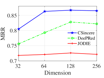
(a) MRR on Reddit

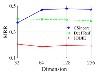
(b) MRR on LastFM

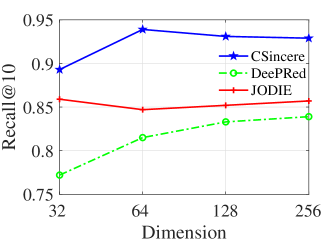
(c) Recall@10 on Reddit

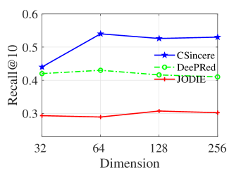
(d) Recall@10 on LastFM

Figure 5: Effect of embedding dimensions

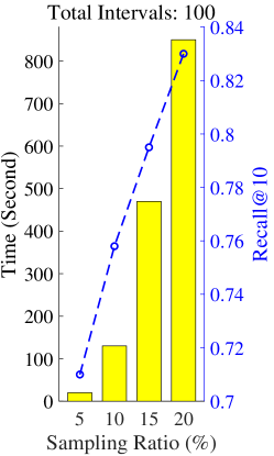
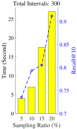
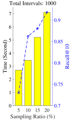
Figure 6: Effect of sample ratio on MOOC dataset.

First, we study the sensitivity of embedding dimension. To this end, the embedding dimension varies in $\{32,64,128,256\}$. (We use $128-$dimensional embeddings as default.) Fig. 5 shows the impact of embedding dimension on the performance of our CSincere, DeePRed and JODIE. As shown in Fig. 5, $128$ seems an optimal value for DeePRed in most cases. JODIE is relatively insensitive to embedding dimension since it counts on the static embeddings [25]. In some cases such as LastFM and Reddit datasets, increasing embedding dimension of CSincere cannot achieve further performance gain by when the dimension is larger than $64$. In these cases, we argue that the $64-$dimensional embedding is already able to capture the information for interaction prediction, owing to the superior expressive power of the Riemannian manifold. However, if we further take the rank information of predicted items into consideration, $128-$dimensional embeddings still obtain a few performance gain, aligned with the intuition. To some extent, it shows the superior expressive volume of Riemannian manifolds, which is also evidenced in [55, 56]. In other words, Riemannian models usually save less computational space in practice.

Second, we study the sampling ratio and the cost of time for computing Ricci curvatures. We set sampling ratio to $20\%$ and use $300$ intervals as default. We summarize the performance of CSincere in Fig. 6, where the yellow bars give the cost of time in seconds, and dashed lines show the prediction results in terms of $Recall@10$. In the experiment, we find that: 1) Higher sampling ratio achieves better results but sharply increases the computing time. That is, curvature estimation is of significance to interaction prediction but it is expensive. 2) The computing time evidently decreases as the number of total intervals increase. In particular, given the sampling ratio set to $20\%$, it costs over $800$ seconds with $100$ intervals, but costs less than $7$ seconds with $1000$ intervals. Such finding suggests that, instead of increasing sampling ratio, higher interval number leads to less time consuming and better prediction results. In other words, we find a solution to tackle with the expensive curvature estimation, using higher interval number.

6 Related Work

6.1 Representation Learning on SIN

Graph representation learning maps each node on a graph to an embedding in the representation space that encodes structure and/or attribute information. Representation learning on SIN considers a bipartite of nodes, and learns node embeddings with a sequence of temporal interactions. In the literature, most previous works study SINs in Euclidean space. Among them, recurrent models routinely find themselves owing to effectiveness on sequential data [20], e.g., Time-LSTM [27], Time-Aware LSTM [28] and RRN [53] model user/item dynamics with gating mechanism for long short-term memory. Random walking is another line for graph representation learning. Concretely, CTDNE [18] extends the random walk to temporal networks. CAW [5] injects the causality to inductively represent sequential networks. Interaction models consider the mutual influence between users and items [17, 19]. HILI [26] is the successor of Jodie [25] and both of them achieve great success. We noticed that researchers explore the representation learning on SIN in hyperbolic spaces. For instance, HyperML [24] learns user/item encodings with the concept of metric learning in the hyperbolic space. HTGN [4] designs a recurrent architecture on the sequence of snapshots under hyperbolic geometric. Also, temporal GNNs achieve great success recently [38, 57, 58, 59], but they are different from the bipartite setting of SINs. Recently, [60] study SIN via a probabilistic model of point process, and [61] propose a novel restart mechanism to improve the efficiency for SIN representation learning.

Please refer to Kazemi et al. [62], Aggarwal and Subbian [63] for a more systematic reviews. Different from the previous studies, we propose the first self-supervised SIN learning model in generic Riemannian manifold, to the best of our knowledge.

6.2 Riemannian Graph Learning

Recently, Riemannian geometry (e.g., hyperbolic and spherical manifolds) emerges as a powerful alternative of the classic Euclidean ones. A series of Riemannian graph models have been proposed. Specifically, on hyperbolic manifolds, shallow models are first introduced [11, 64]. Deep models, i.e., GNNs are then designed with different formulations [65, 66, 10, 33, 34]. On constant-curvature manifolds, $\kappa$-GCN [67] extend GCN to $\kappa$-sterographical model with arbitrary curvature. On ultrahyperbolic manifolds, a kind of pseudo Riemannian manifold, Xiong et al. [68], Xiong et al. [69] present GNNs in the time-space coordinates. On quotient manifolds, Law [70] studies the entanglement of node embedding with some curvature radius. On product manifolds, Gu et al. [71], Wang et al. [72], Skopek et al. [73], Sun et al. [74] explore informative embeddings in the collaboration of different factor manifolds. Additionally, Cruceru et al. [75] study the matrix manifold of Riemannian spaces. Another line of work consider both Riemannian manifold and the Euclidean one. For example, Zhu et al. [76], Yang et al. [42] embed the graph into the dual space of Euclidean and hyperbolic ones simultaneously. Recently, Yang et al. [4] and our previous work [77] model dynamic graphs in hyperbolic manifolds. Sun et al. [78, 79] study the temporal evolvement of the graph in generic Riemannian manifolds. Sun et al. [80] introduces the Riemannian geometry to graph clustering. To the best of our knowledge, we introduce the first co-evolving Riemannian manifolds, aligning with the characteristic of SINs.

7 Conclusion

In this paper, we for the first time study the sequential interaction network learning on co-evolving Riemannian manifolds, and present a novel CSincere. Concretely, we first introduce a co-evolving GNN with two $\kappa-$stereographic space bridged by the common Euclidean tangent space, in which we formulate the cross-space aggregation to conduct message propagation across user space and item space, and design the neural curvature estimator for the space evolvement over time. Thereafter, we propose the Riemannian co-contrastive learning for sequential interaction networks, which in the meanwhile interplays user space and item space for interaction prediction. Finally, extensive experiments on 5 public datasets show CSincere outperforms the state-of-the-art competitors.

References

- \bibcommenthead
- He et al. [2014] He, X., Gao, M., Kan, M.-Y., Liu, Y., Sugiyama, K.: Predicting the popularity of web 2.0 items based on user comments. In: Proceedings of the 37th SIGIR, pp. 233–242 (2014)
- Peng et al. [2021a] Peng, H., Yang, R., Wang, Z., Li, J., He, L., Yu, P., Zomaya, A., Ranjan, R.: Lime: Low-cost incremental learning for dynamic heterogeneous information networks. IEEE Transactions on Computers 71, 628–642 (2021)
- Peng et al. [2021b] Peng, H., Zhang, R., Dou, Y., Yang, R., Zhang, J., Yu, P.S.: Reinforced neighborhood selection guided multi-relational graph neural networks. ACM Transactions on Information Systems 40(69), 1–46 (2021)
- Yang et al. [2021] Yang, M., Zhou, M., Kalander, M., Huang, Z., King, I.: Discrete-time temporal network embedding via implicit hierarchical learning in hyperbolic space. In: Proceedings of KDD, pp. 1975–1985 (2021)
- Wang et al. [2021] Wang, Y., Chang, Y.-Y., Liu, Y., Leskovec, J., Li, P.: Inductive representation learning in temporal networks via causal anonymous walks. In: Proceedings of ICLR (2021)
- Peng et al. [2023, early access] Peng, H., Zhang, R., Li, S., Cao, Y., Pan, S., Yu, P.S.: Reinforced, incremental and cross-lingual event detection from social messages. IEEE Transactions on Pattern Analysis Machine Intelligence (2023, early access)
- Chami et al. [2019] Chami, I., Ying, Z., Ré, C., Leskovec, J.: Hyperbolic graph convolutional neural networks. Advances in NeurIPS 32 (2019)
- Mathieu et al. [2019] Mathieu, E., Le Lan, C., Maddison, C.J., Tomioka, R., Teh, Y.W.: Continuous hierarchical representations with poincaré variational auto-encoders. In: Advances in NeurIPS, pp. 12544–12555 (2019)
- Gulcehre et al. [2019] Gulcehre, C., Denil, M., Malinowski, M., Razavi, A., Pascanu, R., Hermann, K.M., Battaglia, P., Bapst, V., Raposo, D., Santoro, A., Freitas, N.: Hyperbolic attention networks. In: Proceedings of ICLR, pp. 1–15 (2019)
- Zhang et al. [2021] Zhang, Y., Wang, X., Shi, C., Liu, N., Song, G.: Lorentzian graph convolutional networks. In: Proceedings of WWW, pp. 1249–1261 (2021)
- Nickel and Kiela [2017] Nickel, M., Kiela, D.: Poincaré embeddings for learning hierarchical representations. In: Advances in NeurIPS, pp. 6338–6347 (2017)
- Ganea et al. [2018] Ganea, O., Bécigneul, G., Hofmann, T.: Hyperbolic neural networks. In: Advances in NeurIPS, pp. 5345–5355 (2018)
- Defferrard et al. [2020] Defferrard, M., Milani, M., Gusset, F., Perraudin, N.: Deepsphere: a graph-based spherical cnn. In: Proceedings of ICLR (2020)
- Rezende et al. [2020] Rezende, D.J., Papamakarios, G., Racaniere, S., Albergo, M., Kanwar, G., Shanahan, P., Cranmer, K.: Normalizing flows on tori and spheres. In: Proceedings of ICML, pp. 8083–8092 (2020)
- Fan et al. [2021] Fan, Z., Liu, Z., Zhang, J., Xiong, Y., Zheng, L., Yu, P.S.: Continuous-time sequential recommendation with temporal graph collaborative transformer. In: Proceedings of the 30th CIKM, pp. 433–442 (2021)
- Cao et al. [2021] Cao, J., Lin, X., Guo, S., Liu, L., Liu, T., Wang, B.: Bipartite graph embedding via mutual information maximization. In: Proceedings of the 14th CIKM, pp. 635–643 (2021)
- Dai et al. [2016] Dai, H., Wang, Y., Trivedi, R., Song, L.: Deep coevolutionary network: Embedding user and item features for recommendation. arXiv preprint arXiv:1609.03675 (2016)
- Nguyen et al. [2018] Nguyen, G.H., Lee, J.B., Rossi, R.A., Ahmed, N.K., Koh, E., Kim, S.: Continuous-time dynamic network embeddings. In: Companion Proceedings of the Web Conference 2018, pp. 969–976 (2018)
- Kefato et al. [2021] Kefato, Z., Girdzijauskas, S., Sheikh, N., Montresor, A.: Dynamic embeddings for interaction prediction. In: Proceedings of the Web Conference 2021, pp. 1609–1618 (2021)
- Beutel et al. [2018] Beutel, A., Covington, P., Jain, S., Xu, C., Li, J., Gatto, V., Chi, E.H.: Latent cross: Making use of context in recurrent recommender systems. In: Proceedings of the 11th WSDM, pp. 46–54 (2018)
- Sreejith et al. [2016] Sreejith, R., Mohanraj, K., Jost, J., Saucan, E., Samal, A.: Forman curvature for complex networks. Journal of Statistical Mechanics: Theory and Experiment 2016(6), 063206 (2016)
- Bachmann et al. [2020] Bachmann, G., Becigneul, G., Ganea, O.: Constant curvature graph convolutional networks. In: Proceedings of the 37th ICML, vol. 119, pp. 486–496 (2020)
- Gromov [1987] Gromov, M.: In: Gersten, S.M. (ed.) Hyperbolic Groups, pp. 75–263. Springer, New York, NY (1987)
- Vinh Tran et al. [2020] Vinh Tran, L., Tay, Y., Zhang, S., Cong, G., Li, X.: HyperML: A Boosting Metric Learning Approach in Hyperbolic Space for Recommender Systems, pp. 609–617 (2020)
- Kumar et al. [2019] Kumar, S., Zhang, X., Leskovec, J.: Predicting dynamic embedding trajectory in temporal interaction networks. In: Proceedings of the 25th KDD, pp. 1269–1278 (2019)
- Chen et al. [2021] Chen, H., Xiong, Y., Zhu, Y., Yu, P.S.: Highly liquid temporal interaction graph embeddings. In: Proceedings of the Web Conference 2021, pp. 1639–1648 (2021)
- Zhu et al. [2017] Zhu, Y., Li, H., Liao, Y., Wang, B., Guan, Z., Liu, H., Cai, D.: What to do next: Modeling user behaviors by time-lstm. In: Proceedings of the 26th IJCAI, vol. 17, pp. 3602–3608 (2017)
- Baytas et al. [2017] Baytas, I.M., Xiao, C., Zhang, X., Wang, F., Jain, A.K., Zhou, J.: Patient subtyping via time-aware lstm networks. In: Proceedings of the 23rd KDD, pp. 65–74 (2017)
- Ye et al. [2023] Ye, J., Zhang, Z., Sun, L., Yan, Y., Wang, F., Ren, F.: Sincere: Sequential interaction networks representation learning on co-evolving riemannian manifolds. In: Proceedings of ACM The Web Conference (WWW), pp. 1–10 (2023)
- Ungar [2008] Ungar, A.A.: A gyrovector space approach to hyperbolic geometry. Synthesis Lectures on Mathematics and Statistics 1(1), 1–194 (2008)
- Ye et al. [2020] Ye, Z., Liu, K.S., Ma, T., Gao, J., Chen, C.: Curvature graph network. In: Proceedings of ICLR (2020)
- Lee [2018] Lee, J.M.: Introduction to Riemannian Manifolds, (2018)
- Dai et al. [2021] Dai, J., Wu, Y., Gao, Z., Jia, Y.: A hyperbolic-to-hyperbolic graph convolutional network. In: Proceedings of CVPR, pp. 154–163 (2021)
- Chen et al. [2022] Chen, W., Han, X., Lin, Y., Zhao, H., Liu, Z., Li, P., Sun, M., Zhou, J.: Fully hyperbolic neural networks. In: Proceedings of the 60th ACL, pp. 5672–5686 (2022)
- Ollivier [2009] Ollivier, Y.: Ricci curvature of markov chains on metric spaces. Journal of Functional Analysis 256(3), 810–864 (2009)
- Forman [2003] Forman, R.: Bochner’s method for cell complexes and combinatorial ricci curvature. Discrete and Computational Geometry 29(3), 323–374 (2003)
- Ungar [2010] Ungar, A.A.: Barycentric Calculus in Euclidean and Hyperbolic Geometry: A Comparative Introduction, (2010)
- Xu et al. [2020] Xu, D., Ruan, C., Korpeoglu, E., Kumar, S., Achan, K.: Inductive representation learning on temporal graphs. In: Proceedings of ICLR (2020)
- Sia et al. [2019] Sia, J., Jonckheere, E., Bogdan, P.: Ollivier-ricci curvature-based method to community detection in complex networks. Scientific reports 9(1), 1–12 (2019)
- Gu et al. [2019] Gu, A., Sala, F., Gunel, B., Re, C.: Learning mixed-curvature representations in product spaces. In: Proceedings of ICLR (2019)
- Fu et al. [2021] Fu, X., Li, J., Wu, J., Sun, Q., Ji, C., Wang, S., Tan, J., Peng, H., Yu, P.S.: Ace-hgnn: Adaptive curvature exploration hyperbolic graph neural network. In: Proceedings of ICDM, pp. 111–120 (2021)
- Yang et al. [2022] Yang, H., Chen, H., Pan, S., Li, L., Yu, P.S., Xu, G.: Dual space graph contrastive learning. In: Proceedings of The ACM Web Conference, pp. 1238–1247 (2022)
- Hassani and Ahmadi [2020] Hassani, K., Ahmadi, A.H.K.: Contrastive multi-view representation learning on graphs. In: Proceedings of ICML, vol. 119, pp. 4116–4126 (2020)
- Qiu et al. [2020] Qiu, J., Chen, Q., Dong, Y., Zhang, J., Yang, H., Ding, M., Wang, K., Tang, J.: GCC: graph contrastive coding for graph neural network pre-training. In: Proceedings of KDD, pp. 1150–1160 (2020)
- Sun et al. [2022] Sun, L., Ye, J., Peng, H., Yu, P.S.: A self-supervised riemannian GNN with time varying curvature for temporal graph learning. In: Proceedings of the 31st CIKM, pp. 1827–1836 (2022)
- Tian et al. [2021] Tian, S., Wu, R., Shi, L., Zhu, L., Xiong, T.: Self-supervised representation learning on dynamic graphs. In: Proceedings of the 30th CIKM, pp. 1814–1823 (2021)
- Oord et al. [2018] Oord, A.v.d., Li, Y., Vinyals, O.: Representation learning with contrastive predictive coding. arXiv: 1807.03748, 1–13 (2018)
- Veličković et al. [2019] Veličković, P., Fedus, W., Hamilton, W.L., Liò, P., Bengio, Y., Hjelm, R.D.: Deep graph infomax. In: Proceedings of ICLR, pp. 1–24 (2019)
- Robinson et al. [2021] Robinson, J.D., Chuang, C., Sra, S., Jegelka, S.: Contrastive learning with hard negative samples. In: Proceedings of the 9th ICLR (2021)
- Xia et al. [2022] Xia, J., Wu, L., Wang, G., Chen, J., Li, S.Z.: Progcl: Rethinking hard negative mining in graph contrastive learning. In: Proceedings of ICML, vol. 162, pp. 24332–24346 (2022)
- Ni et al. [2019] Ni, C., Lin, Y., Luo, F., Gao, J.: Community detection on networks with ricci flow. Nature Scientific Reports 9(9984) (2019)
- Ye et al. [2020] Ye, Z., Liu, K.S., Ma, T., Gao, J., Chen, C.: Curvature graph network. In: Proceedings of the 8th ICLR (2020)
- Wu et al. [2017] Wu, C.-Y., Ahmed, A., Beutel, A., Smola, A.J., Jing, H.: Recurrent recommender networks. In: Proceedings of the 10th WSDM, pp. 495–503 (2017)
- Sun et al. [2021] Sun, J., Cheng, Z., Zuberi, S., Perez, F., Volkovs, M.: Hgcf: Hyperbolic graph convolution networks for collaborative filtering. In: Proceedings of the Web Conference 2021, pp. 593–601 (2021)
- Shimizu et al. [2021] Shimizu, R., Mukuta, Y., Harada, T.: Hyperbolic neural networks++. In: Proceedings of ICLR, pp. 1–25 (2021)
- Lee [2013] Lee, J.M.: Introduction to Smooth Manifolds (2nd Edition), (2013)
- Wang et al. [2021] Wang, Y., Cai, Y., Liang, Y., Ding, H., Wang, C., Bhatia, S., Hooi, B.: Adaptive data augmentation on temporal graphs. In: Advances in NeurIPS, vol. 34, pp. 1440–1452 (2021)
- Zuo et al. [2018] Zuo, Y., Liu, G., Lin, H., Guo, J., Hu, X., Wu, J.: Embedding temporal network via neighborhood formation. In: Proceedings of KDD, pp. 2857–2866 (2018)
- Gupta et al. [2022] Gupta, S., Manchanda, S., Bedathur, S., Ranu, S.: Tigger: Scalable generative modelling for temporal interaction graphs. In: Proceedings of AAAI, vol. 36, pp. 6819–6828 (2022)
- Xia et al. [2023] Xia, W., Li, Y., Li, S.: Graph neural point process for temporal interaction prediction. IEEE Transactions on Knowledge and Data Engineering 35(5), 4867–4879 (2023)
- Zhang et al. [2023] Zhang, Y., Xiong, Y., Liao, Y., Sun, Y., Jin, Y., Zheng, X., Zhu, Y.: TIGER: temporal interaction graph embedding with restarts. In: Proceedings of the ACM Web Conference 2023 (WWW), pp. 478–488 (2023)
- Kazemi et al. [2020] Kazemi, S.M., Goel, R., Jain, K., Kobyzev, I., Sethi, A., Forsyth, P., Poupart, P.: Representation learning for dynamic graphs: A survey. Journal of Machine Learning Research 21(70), 1–73 (2020)
- Aggarwal and Subbian [2014] Aggarwal, C., Subbian, K.: Evolutionary network analysis: A survey. ACM Computing Surveys (CSUR) 47(1), 1–36 (2014)
- Suzuki et al. [2019] Suzuki, R., Takahama, R., Onoda, S.: Hyperbolic disk embeddings for directed acyclic graphs. In: Proceedings of ICML, pp. 6066–6075 (2019)
- Chami et al. [2019] Chami, I., Ying, Z., Ré, C., Leskovec, J.: Hyperbolic graph convolutional neural networks. In: Advances in NeurIPS, pp. 4869–4880 (2019)
- Liu et al. [2019] Liu, Q., Nickel, M., Kiela, D.: Hyperbolic graph neural networks. In: Advances in NeurIPS, pp. 8228–8239 (2019)
- Bachmann et al. [2020] Bachmann, G., Bécigneul, G., Ganea, O.: Constant curvature graph convolutional networks. In: Proceedings of ICML, vol. 119, pp. 486–496 (2020)
- Xiong et al. [2022a] Xiong, B., Zhu, S., Nayyeri, M., Xu, C., Pan, S., Zhou, C., Staab, S.: Ultrahyperbolic knowledge graph embeddings. In: Proceedings of KDD, pp. 2130–2139 (2022)
- Xiong et al. [2022b] Xiong, B., Zhu, S., Potyka, N., Pan, S., Zhu, C., Staab, S.: Pseudo-riemannian graph convolutional networks. In: Advances in 36th NeurIPS, pp. 1–21 (2022)
- Law [2021] Law, M.: Ultrahyperbolic neural networks. In: Advances in NeurIPS, vol. 34, pp. 22058–22069 (2021)
- Gu et al. [2019] Gu, A., Sala, F., Gunel, B., Ré, C.: Learning mixed-curvature representations in product spaces. In: Proceedings of ICLR, pp. 1–21 (2019)
- Wang et al. [2021] Wang, S., Wei, X., Santos, C.N., Wang, Z., Nallapati, R., Arnold, A.O., Xiang, B., Yu, P.S., Cruz, I.F.: Mixed-curvature multi-relational graph neural network for knowledge graph completion. In: Proceedings of The ACM Web Conference, pp. 1761–1771 (2021)
- Skopek et al. [2020] Skopek, O., Ganea, O.-E., Becigneul, G.: Mixed-curvature variational autoencoders. In: Proceedings of ICLR (2020)
- Sun et al. [2022] Sun, L., Zhang, Z., Ye, J., Peng, H., Zhang, J., Su, S., Yu, P.S.: A self-supervised mixed-curvature graph neural network. In: Proceedings of AAAI, vol. 36, pp. 4146–4155 (2022)
- Cruceru et al. [2021] Cruceru, C., Bécigneul, G., Ganea, O.: Computationally tractable riemannian manifolds for graph embeddings. In: Proceedings of AAAI, pp. 7133–7141 (2021)
- Zhu et al. [2020] Zhu, S., Pan, S., Zhou, C., Wu, J., Cao, Y., Wang, B.: Graph geometry interaction learning. In: Advances in NeurIPS, vol. 33, pp. 7548–7558 (2020)
- Sun et al. [2021] Sun, L., Zhang, Z., Zhang, J., Wang, F., Peng, H., Su, S., Yu, P.S.: Hyperbolic variational graph neural network for modeling dynamic graphs. In: Proceedings of the 35th AAAI, pp. 4375–4383 (2021)
- Sun et al. [2023] Sun, L., Ye, J., Peng, H., Wang, F., Yu, P.S.: Self-supervised continual graph learning in adaptive riemannian spaces. In: Proceedings of the 37th AAAI, pp. 4633–4642 (2023)
- Sun et al. [2022] Sun, L., Ye, J., Peng, H., Yu, P.S.: A self-supervised riemannian GNN with time varying curvature for temporal graph learning. In: Proceedings of the 31st CIKM, pp. 1827–1836 (2022)
- Sun et al. [2023] Sun, L., Wang, F., Ye, J., Peng, H., Yu, P.S.: CONGREGATE: contrastive graph clustering in curvature spaces. In: Proceedings of the 32nd IJCAI, pp. 2296–2305 (2023)