Polynomial Fourier decay for fractal measures and their pushforwards

Abstract.

We prove that the pushforwards of a very general class of fractal measures $\mu$ on $\mathbb{R}^{d}$ under a large family of non-linear maps $F\colon\mathbb{R}^{d}\to\mathbb{R}$ exhibit polynomial Fourier decay: there exist $C,\eta>0$ such that $|\widehat{F\mu}(\xi)|\leq C|\xi|^{-\eta}$ for all $\xi\neq 0$. Using this, we prove that if $\Phi=\{\varphi_{a}\colon[0,1]\to[0,1]\}_{a\in\mathcal{A}}$ is an iterated function system consisting of analytic contractions, and there exists $a\in\mathcal{A}$ such that $\varphi_{a}$ is not an affine map, then every non-atomic self-conformal measure for $\Phi$ has polynomial Fourier decay; this result was obtained simultaneously by Algom, Rodriguez Hertz, and Wang. We prove applications related to the Fourier uniqueness problem, Fractal Uncertainty Principles, and normal numbers in fractal sets.

Mathematics Subject Classification 2020: 42A38 (Primary), 28A80, 60F10 (Secondary)

Key words and phrases: Fourier transform, self-conformal measure, non-linear images

1. Introduction

1.1. Background and results

The Fourier transform of a Borel probability measure $\mu$ supported on $\mathbb{R}$ is the function $\widehat{\mu}\colon\mathbb{R}\to\mathbb{C}$ given by

(1.1) $$\widehat{\mu}(\xi)=\int_{\mathbb{R}}e^{-2\pi i\xi x}d\mu(x).$$

It is an important quantity giving ‘arithmetic’ information about the measure. However, it is often difficult to calculate. A measure $\mu$ is said to be a Rajchman measure if $\widehat{\mu}(\xi)\to 0$ as $|\xi|\to\infty$. Determining whether a measure is Rajchman, and if it is Rajchman, the speed at which the Fourier transform converges to zero, is an interesting and important problem.

In this paper we consider this problem in the context of fractal measures. Historically, the study of the Fourier transform of fractal measures was initiated by problems coming from uniqueness of trigonometric series, metric number theory, Fourier multipliers, and maximal operators defined by fractal measures. We refer the reader to [43, 44] for a thorough historical overview. Well studied families of fractal measures include the self-similar measures and self-conformal measures; these arise from iterated function systems, which are defined as follows. We call a map $\varphi\colon[0,1]^{d}\to[0,1]^{d}$ a contraction if there exists $r\in(0,1)$ such that $\|\varphi(x)-\varphi(y)\|\leq r\|x-y\|$ for all $x,y\in[0,1]^{d}$. We call a finite set of contractions an iterated function system, or IFS for short. A well-known result due to Hutchinson [35] states that for any IFS $\Phi=\{\varphi_{a}\}_{a\in\mathcal{A}}$, there exists a unique non-empty compact set $X$ satisfying

$$X=\bigcup_{a\in\mathcal{A}}\varphi_{a}(X).$$

We call $X$ the attractor of $\Phi$. We will always assume that our IFS is non-trivial, by which we mean that the contractions do not all share a common fixed point, and thus $X$ is always uncountable. The attractors of iterated function systems often exhibit fractal behaviour. To understand the metric properties of an attractor $X$, one typically studies measures supported on $X$. The most well studied fractal measures are the stationary measures arising from probability vectors (see [32, 57, 63]). Given an IFS $\Phi=\{\varphi_{a}\}_{a\in\mathcal{A}}$ and a probability vector $\mathbf{p}=(p_{a})_{a\in\mathcal{A}}$ ($0<p_{a}<1$ for all $a$ and $\sum_{a\in\mathcal{A}}p_{a}=1$), another well-known result, also due to Hutchinson [35], states that there exists a unique Borel probability measure satisfying

(1.2) $$\mu=\sum_{a\in\mathcal{A}}p_{a}\cdot\varphi_{a}\mu.$$

We call $\mu$ the stationary measure corresponding to $\Phi$ and $\mathbf{p}$, and emphasise that we always assume that all probability weights are strictly positive. Recall that a map $\varphi\colon[0,1]^{d}\to[0,1]^{d}$ is called a similarity if there exists $r\in(0,1)$ such that $\|\varphi(x)-\varphi(y)\|=r\|x-y\|$ for all $x,y\in[0,1]^{d}$. If an IFS $\Phi$ consists of similarities, and we want to emphasise this property, then we say that the IFS is a self-similar iterated function system, and the corresponding stationary measures are known as self-similar measures. Similarly, if $\Phi$ consists of $C^{1+\alpha}$ angle-preserving contractions, then the IFS is called a self-conformal IFS, and the corresponding stationary measures are known as self-conformal measures. Self-conformal IFSs and self-conformal measures arise naturally in several areas of mathematics. They appear in number theory by considering the inverse branches of the Gauss map [36]. Similarly, the Furstenberg measures that play an important role in random matrix theory can under suitable hypothesis be realised as self-conformal measures [8, 66].

Understanding the Fourier decay properties of stationary measures for IFSs is an active area of research; see [53] for a recent survey, which also discusses several applications of this problem. This problem has received a particularly large amount of attention in the context of self-similar measures and self-conformal measures. In particular, much emphasis has been put on understanding when the number theoretic properties of a self-similar IFS influence the Fourier decay of the corresponding self-similar measures. Some of the first contributions in this area are due to Erdős [26, 27]. In these papers he studied the self-similar measures corresponding to the IFS $\{\varphi_{0}(x)=\lambda x-1,\varphi_{1}(x)=\lambda x+1\}$ and the $(1/2,1/2)$ probability vector, where $\lambda\in(1/2,1)$. These self-similar measures, which we denote by $\mu_{\lambda}$, are the well studied Bernoulli convolutions (see [62, 63] for surveys on this topic). In [26], Erdős showed that whenever $\lambda$ is the reciprocal of a Pisot number, $\mu_{\lambda}$ is singular with respect to the Lebesgue measure; he proved this by showing that $\mu_{\lambda}$ is not Rajchman and applying the Riemann–Lebesgue lemma. In [27], he proved that for all $m\in\mathbb{N}$ there exists $\delta_{m}>0$ such that for Lebesgue almost every $\lambda\in(1-\delta_{m},1)$, the measure $\mu_{\lambda}$ is absolutely continuous and the corresponding density is $m$-times differentiable. Erdős proved this result by establishing that for Lebesgue almost every $\lambda\in(1-\delta_{m},1)$, the Fourier transform of $\mu_{\lambda}$ converges to zero sufficiently quickly. Erdős’ Fourier transform method was subsequently refined by Kahane [38], who used it to bound the Hausdorff dimension of the set of $\lambda$ in a small neighbourhood of $1$ for which $\mu_{\lambda}$ is singular with respect to the Lebesgue measure.

More recently, in [59] Solomyak proved that outside of a set of parameters of Hausdorff dimension zero, all self-similar measures supported on the line have polynomial Fourier decay, by which we mean there exist $C,\eta>0$ such that $|\widehat{\mu}(\xi)|\leq C|\xi|^{-\eta}$ for all $\xi\neq 0$. Despite this result, obtaining explicit examples of self-similar measures exhibiting polynomial Fourier decay is a difficult problem; the only non-trivial examples are due to Dai, Feng, and Wang [20] and Streck [58]. In [43], Li and Sahlsten obtained a decay rate for the Fourier transform of certain self-similar measures. They proved that if a self-similar IFS contains two maps which satisfy a mild Diophantine assumption, then every self-similar measure exhibits logarithmic Fourier decay, i.e. there exist $C,\eta>0$ such that $|\widehat{\mu}(\xi)|\leq C(\log|\xi|)^{-\eta}$ whenever $|\xi|>1$. In [3] Algom, Rodriguez Hertz, and Wang considered a related Diophantine condition; they showed that if a self-similar IFS satisfies this condition then every self-similar measure has logarithmic Fourier decay. The Diophantine condition considered in [3] covers examples of self-similar IFSs that are not covered by [43] (see [3, Section 6.3]). Building upon work of Brémont [16], Varjú and Yu similarly proved that for a certain class of self-similar iterated function systems, if the IFS cannot be conjugated to an IFS whose contraction ratios are a special type of algebraic number, then every self-similar measure exhibits logarithmic Fourier decay [64]. If one does not ask for a quantitative decay rate for the Fourier transform of a self-similar measure then much more is known. Rapaport [51] has given an algebraic characterisation of IFSs acting on $\mathbb{R}^{d}$ that admit a self-similar measure which is not Rajchman.

For self-conformal measures, on the other hand, it is generally believed that if the underlying IFS is sufficiently non-linear then the measure will exhibit polynomial Fourier decay. This line of research was taken up by Jordan and Sahlsten [36] who, building upon work of Kaufman [39], and later Queffélec and Ramaré [50], proved that if $\mu$ is a Gibbs measure for the Gauss map of sufficiently large dimension then the Fourier transform of $\mu$ has polynomial Fourier decay. This result was then generalised by Bourgain and Dyatlov in [15], who used methods from additive combinatorics to establish polynomial Fourier decay for Patterson–Sullivan measures for convex cocompact Fuchsian groups. The additive combinatorics methods of Bourgain and Dyatlov were later applied by Sahlsten and Stevens in [54]. In this paper they proved that Gibbs measures for well separated self-conformal IFSs acting on the line satisfying a suitable non-linearity assumption have polynomial Fourier decay. Algom, Rodriguez Hertz, and Wang [3, 4] established weaker decay rates for the Fourier transform of self-conformal measures under weaker assumptions than those appearing in [54]. Recently both the first named author and Sahlsten [10], and Algom, Rodriguez Hertz, and Wang [5], gave sufficient conditions on an IFS which guarantee that every self-conformal measure exhibits polynomial Fourier decay. Both of these papers used a disintegration method inspired by work of Algom, the first named author, and Shmerkin [1], albeit in different ways. Importantly, the results in [3, 4, 5, 10] do not require the IFS to satisfy any separation assumptions.

In this paper we prove that a self-conformal measure coming from an IFS consisting of analytic maps will have polynomial Fourier decay under the weakest possible non-linearity assumption. In particular, the following holds.

Theorem 1.1.

Let $\{\varphi_{a}\colon[0,1]\to[0,1]\}_{a\in\mathcal{A}}$ be a non-trivial IFS such that each $\varphi_{a}$ is analytic, and suppose that there exists $a\in\mathcal{A}$ such that $\varphi_{a}$ is not an affine map. Then for every self-conformal measure $\mu$ there exist $C,\eta>0$ such that $|\widehat{\mu}(\xi)|\leq C|\xi|^{-\eta}$ for all $\xi\neq 0$.

Theorem 1.1 was obtained simultaneously and independently by Algom et al. in [2]. This theorem was announced in [5] and in [5, Section 6] a short argument, conditional on what was at the time a forthcoming result of Algom et al. [2] (which also follows from this paper), was provided.

The proof of Theorem 1.1 divides into two cases depending on whether or not the IFS admits an analytic conjugacy to a self-similar IFS; both cases are highly non-trivial. The case where no such conjugacy exists follows from the main results in [5] and [10], which are proved by establishing spectral gap-type estimates for appropriate transfer operators. For the case where the IFS admits such a conjugacy, the corresponding self-conformal measures can be realised as pushforwards of self-similar measures under the conjugacy map. Using this observation, the conjugacy case of Theorem 1.1 follows from a suitable result on the behaviour of non-linear pushforwards. In particular, this case follows from Theorem 1.4 (see the argument given in Section 3). Similarly, a suitable theorem on the behaviour on non-linear pushforwards of self-conformal measures was obtained by Algom et al. in [2]. It was this result that was relied upon in the conditional argument given in [5].

The present paper and [2] differ in two key ways. Whereas [5], [10] and this paper made use of a disintegration technique from [1] to establish Fourier decay, Algom et al. [2] use a large deviations estimate of Tsujii [61]. Our non-linear projection theorem applies more generally and covers some higher-dimensional and infinite iterated function systems. On the other hand, the non-linear projection theorem of Algom et al. is a more direct analogue of the classical van der Corput inequality from harmonic analysis. They also use this theorem to prove equidistribution results for the sequence $(x^{n}\mod 1)_{n=1}^{\infty}$, where $x$ is distributed according to a self-similar measure.

1.2. Non-linear pushforwards of fractal measures

Our results on non-linear pushforwards of fractal measures hold in the general setting of countable IFSs, which were studied systematically in [45]. As such it is necessary to introduce some additional terminology. We call a countable family $\Phi=\{\varphi_{a}\colon[0,1]^{d}\to[0,1]^{d}\}_{a\in\mathcal{A}}$ of contractions satisfying

$$\sup_{a\in\mathcal{A}}\sup_{x,y\in[0,1]^{d}}\frac{\|\varphi_{a}(x)-\varphi_{a}(y)\|}{\|x-y\|}<1$$

a countable iterated function system, or CIFS for short. For a countable iterated function system there no longer necessarily exists a unique non-empty compact set $X$ satisfying $X=\cup_{a\in\mathcal{A}}\varphi_{a}(X)$. As such, given a CIFS we define

$$X\coloneqq\bigcup_{(a_{i})_{i=1}^{\infty}\in\mathcal{A}^{\mathbb{N}}}\bigcap_{n=1}^{\infty}(\varphi_{a_{1}}\circ\cdots\circ\varphi_{a_{n}})([0,1]^{d}),$$

and call $X$ the attractor of $\Phi$. When our countable IFS contains finitely many contractions, i.e. it is an IFS, then the attractor as defined above coincides with the unique non-empty compact set satisfying $X=\cup_{a\in\mathcal{A}}\varphi_{a}(X)$, so there is no ambiguity in our use of the term attractor. Given a CIFS $\Phi=\{\varphi_{a}\}_{a\in\mathcal{A}}$ and a probability vector $\mathbf{p}=(p_{a})_{a\in\mathcal{A}}$ there exists a unique Borel probability measure satisfying

$$\mu=\sum_{a\in\mathcal{A}}p_{a}\cdot\varphi_{a}\mu.$$

We call $\mu$ the stationary measure for $\Phi$ and $\mathbf{p}$.

In this paper we will focus on the stationary measures coming from the following special class of CIFSs.

Definition 1.2.

Let $\Psi\coloneqq\{\psi_{j}\colon[0,1]^{d}\to[0,1]^{d}\}_{j\in J}$ be a CIFS. Suppose that for each $j\in J$ there exists a CIFS $\Psi_{j}\coloneqq\{\gamma_{l,j}\colon[0,1]\to[0,1]\}_{l\in L_{j}}$. Then we define the fibre product CIFS (consisting of maps from $[0,1]^{d+1}$ to itself) to be

$$\Phi=\left\{\varphi_{j,l}(x_{1},\ldots,x_{d+1})=(\psi_{j}(x_{1},\ldots,x_{d}),\gamma_{l,j}(x_{d+1}))\right\}_{j\in J,l\in L_{j}}.$$

We refer to $\Psi$ as the base CIFS, and to each $\Psi_{j}$ as a fibre CIFS. We will always assume that the fibre product IFS is itself a CIFS, so satisfies the condition

$$\sup_{j,l}\sup_{x,y\in[0,1]^{d+1}}\frac{\|\varphi_{j,l}(x)-\varphi_{j,l}(y)\|}{\|x-y\|}<1.$$

To illustrate how general this definition is, we note that a very special subclass of fibre product IFSs are the IFSs consisting of finitely many affine contractions on $[0,1]^{d}$ whose linear parts are given by diagonal matrices. Attractors of IFSs in this subclass include self-similar or self-affine carpets and sponges such as those of Barański [11], Bedford–McMullen [13, 46], or Gatzouras–Lalley [31] type. Some more detailed examples are given in Figure 1.

Given a $C^{2}$ function $F\colon[0,1]^{d+1}\to\mathbb{R}$, we associate the quantities

$$\|F\|_{\infty,1}\coloneqq\max_{x\in[0,1]^{d+1}}\left|\frac{\partial F}{\partial x_{d+1}}(x)\right|,\quad\|F\|_{\infty,2}\coloneqq\max_{x\in[0,1]^{d+1}}\left|\frac{\partial^{2}F}{\partial x_{d+1}^{2}}(x)\right|$$

and

$$\|F\|_{\min,2}\coloneqq\min_{x\in[0,1]^{d+1}}\left|\frac{\partial^{2}F}{\partial x_{d+1}^{2}}(x)\right|.$$

Our main result for non-linear pushforwards of fractal measures is Theorem 1.3. It is proved in Section 4, which constitutes much of the work in this paper.

Theorem 1.3.

Let $\Phi$ be a fibre product IFS for some $\Psi=\{\psi_{j}\}_{j\in J}$ and $\{\Psi_{j}\}_{j\in J}$. Suppose that $\Phi$ satisfies the following properties:

1. Each fibre CIFS consists of similarities, i.e. each $\Psi_{j}$ has the form $\Psi_{j}=\{\gamma_{l,j}(x)=r_{l,j}\cdot x+t_{l,j}\}_{l\in L_{j}}$ where $|r_{l,j}|\in(0,1)$ and $t_{l,j}\in\mathbb{R}$.

2. There exists a fibre CIFS $\Psi_{j^{*}}$ such that the corresponding attractor is not a singleton.

Let $\mathbf{p}=(p_{j,l})_{j\in J,l\in L_{j}}$ be a probability vector and assume that there exists $\tau>0$ such that

(1.3) $$\sum_{j\in J}\sum_{l\in L_{j}}p_{j,l}|r_{j,l}|^{-\tau}<\infty.$$

Let $\mu$ be the stationary measure for $\Phi$ and $\mathbf{p}$. Then there exist $\eta,\kappa,C>0$ such that for all $C^{2}$ functions $F\colon[0,1]^{d+1}\to\mathbb{R}$ which satisfy $\frac{\partial^{2}F}{\partial x_{d+1}^{2}}(x)\neq 0$ for all $x\in[0,1]^{d+1}$, we have

$$|\widehat{F\mu}(\xi)|\leq C(1+\|F\|_{\infty,1}+\|F\|_{\infty,1}^{-\kappa}+\|F\|_{\infty,2})(1+\|F\|_{\min,2}^{-\kappa})|\xi|^{-\eta}\quad\mbox{ for all }\xi\neq 0.$$

In particular, given a $C^{2}$ function $F\colon[0,1]^{d+1}\to\mathbb{R}$ which satisfies $\frac{\partial^{2}F}{\partial x_{d+1}^{2}}(x)\neq 0$ for all $x\in[0,1]^{d+1}$, there exists $C_{F,\mu}>0$ depending upon $F$ and $\mu$ such that

$$|\widehat{F\mu}(\xi)|\leq C_{F,\mu}|\xi|^{-\eta}\quad\mbox{ for all }\xi\neq 0.$$

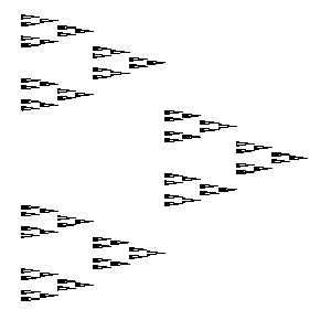
(a)

(b)

(c)

Figure 1. Let
$\displaystyle\Phi_{1}=$ $\displaystyle\Big{\{}\varphi_{1}(x,y)=\Big{(}\frac{x}{2},\frac{y}{3}\Big{)},\,\varphi_{2}(x,y)=\Big{(}\frac{x}{2},\frac{y+2}{3}\Big{)},\,\varphi_{3}(x,y)=\Big{(}\frac{x+1}{2},\frac{y+1}{3}\Big{)}\Big{\}},$ $\displaystyle\Phi_{2}=$ $\displaystyle\Big{\{}\varphi_{1}(x,y)=\Big{(}\frac{x}{3},\frac{y}{5}\Big{)},\,\varphi_{2}(x,y)=\Big{(}\frac{x}{3},\frac{4y+5}{10}\Big{)},\,\varphi_{3}(x,y)=\Big{(}\frac{x+1}{2},\frac{y+1}{2}\Big{)},$ $\displaystyle\varphi_{4}(x,y)=\Big{(}\frac{x+2}{5},\frac{9y}{10}\Big{)},\,\varphi_{5}(x,y)=\Big{(}\frac{7x+1}{10},\frac{3y+6}{10}\Big{)},\,\varphi_{6}(x,y)=\Big{(}\frac{3x+6}{10},\frac{2x+2}{5}\Big{)}\Big{\}},$ $\displaystyle\Phi_{3}=$ $\displaystyle\Big{\{}\varphi_{1}(x,y)=\Big{(}\frac{x}{3},\frac{y}{5}\Big{)},\,\varphi_{2}(x,y)=\Big{(}\frac{x+1}{3},\frac{y+2}{5}\Big{)},\,\varphi_{3}(x,y)=\Big{(}\frac{x+2}{3},\frac{y+4}{5}\Big{)}\Big{\}}.$ The attractor for $\Phi_{1}$ is a Bedford–McMullen carpet to which Theorem 1.3 can be applied, and $\Phi_{2}$ is an overlapping IFS to which Theorem 1.3 applies. Notice that for both $\Phi_{1}$ and $\Phi_{2}$ the maps $\varphi_{1}$ and $\varphi_{2}$ have the same horizontal component but have vertical components with distinct fixed points. Therefore $\Phi_{1}$ and $\Phi_{2}$ satisfy condition (2) in the statement of Theorem 1.3. Notice however that $\Phi_{3}$ is an IFS which fails this condition.

Theorem 1.3 immediately implies the following statement for stationary measures for a CIFS consisting of similarities acting on $[0,1]$.

Theorem 1.4.

Let $\Phi$ be a non-trivial countable IFS acting on $[0,1]$ consisting of similarities, and let $\mathbf{p}$ be a probability vector. Assume that

$$\sum_{a\in\mathcal{A}}p_{a}|r_{a}|^{-\tau}<\infty$$

for some $\tau>0$. Let $\mu$ be the stationary measure for $\Phi$ and $\mathbf{p}$. Then there exist $\eta,\kappa,C>0$ such that for all $C^{2}$ functions $F\colon[0,1]\to\mathbb{R}$ which satisfy $F^{\prime\prime}(x)\neq 0$ for all $x\in[0,1]$, we have

$$|\widehat{F\mu}(\xi)|\leq C(1+\max_{x\in[0,1]}|F^{\prime}(x)|+\max_{x\in[0,1]}|F^{\prime}(x)|^{-\kappa}+\max_{x\in[0,1]}|F^{\prime\prime}(x)|)(1+\min_{x\in[0,1]}|F^{\prime\prime}(x)|^{-\kappa})|\xi|^{-\eta}$$

for all $\xi\neq 0$.

In particular, given a $C^{2}$ function $F\colon[0,1]\to\mathbb{R}$ which satisfies $F^{\prime\prime}(x)\neq 0$ for all $x\in[0,1]$, there exists $C_{F,\mu}>0$ depending upon $F$ and $\mu$ such that

$$|\widehat{F\mu}(\xi)|\leq C_{F,\mu}|\xi|^{-\eta}\quad\mbox{ for all }\xi\neq 0.$$

Proof.

Let $\Phi=\{\varphi_{a}\}_{a\in\mathcal{A}}$ and $\mathbf{p}$ respectively be a CIFS and probability vector satisfying our assumptions, and let $\mu$ be the corresponding stationary measure. Let $\Psi=\{\psi_{0}\}$ be the single element self-similar IFS acting on $\mathbb{R}$ consisting of the map $\psi_{0}(x)=x/2$. Let $\Psi_{0}=\{\varphi_{a}\}_{a\in\mathcal{A}}$ and $\tilde{\Phi}$ be the corresponding fibre product IFS. Let $\nu$ be the stationary measure (on $\mathbb{R}^{2}$) corresponding to $\tilde{\Phi}$ and $\mathbf{p}$. It is straightforward to verify that $\nu=\delta_{0}\times\mu$, where $\delta_{0}$ is the Dirac mass at $0$.

Now let $F\colon[0,1]\to\mathbb{R}$ be a $C^{2}$ function satisfying $F^{\prime\prime}(x)\neq 0$ for all $x\in[0,1]$. We define $\tilde{F}\colon[0,1]^{2}\to\mathbb{R}$ by $\tilde{F}(x,y)=F(y)$. Then $\tilde{F}\nu=F\mu$. Now applying Theorem 1.3 for $\tilde{F}$ and $\nu$ implies the desired statements for $F$ and $\mu$. ∎

We now make several comments about the statement of Theorems 1.3 and 1.4. The first part of Theorem 1.4 will be used in an important way in our proof of Theorem 1.1. The bound involving the $\max_{x\in[0,1]}|F^{\prime}(x)|,\max_{x\in[0,1]}|F^{\prime\prime}(x)|$ and $\min_{x\in[0,1]}|F^{\prime}(x)|$ terms will be sufficiently flexible to allow us to control pushforwards where the underlying $F$ may satisfy $F^{\prime\prime}(x)=0$ for some $x\in[0,1]$. The second part of Theorem 1.4 in the special case of self-similar measures for a finite IFS has been obtained independently and simultaneously by Algom et al in [2], using a somewhat different method. The second part of Theorem 1.4 generalises earlier work of Mosquera and Shmerkin [47, Theorem 3.1], and Chang and Gao [18], who both independently proved Theorem 1.4 under the additional assumption that the CIFS consists of finitely many similarities all with the same contraction ratio. These results were themselves generalisations of previous work of Kaufman [40] who proved the corresponding result for Bernoulli convolutions.

As well as holding for finite IFSs, Theorems 1.3 and 1.4 hold for CIFSs, where the condition (1.3) is important as it allows us to apply Cramér’s theorem for large deviations. This condition also implies that the Lyapunov exponent $\Lambda$ is finite, where

$$\Lambda\coloneqq\sum_{j\in J}\sum_{l\in L_{j}}p_{l,j}\log|r_{l,j}^{-1}|.$$

We emphasise that we do not assume that the CIFS satisfies any homogeneity or separation assumptions (a well-studied example of a CIFS of similarities which does satisfy nice properties is the Lüroth maps). We also emphasise that the base CIFS $\Psi$ can be an arbitrary CIFS (the contractions do not need to be “nice” maps). The constants $\eta,\kappa,C>0$ do not depend upon the choice of $F$ and only depend upon the underlying CIFS and probability vector. Given a particular CIFS, one could carefully follow the proof to make the constant $\eta$ explicit. However, this argument does not yield a general formula for $\eta$, and as such we will not pursue this here.

1.3. Structure of the paper

In Section 2 we prove several applications, assuming Theorems 1.1 and 1.3. These applications relate to the Fourier uniqueness problem, Fractal Uncertainty Principles, and normal numbers in fractal sets. In Section 3 we prove Theorem 1.1 assuming Theorem 1.3. In Section 4 we prove Theorem 1.3; an informal outline of the proof, which involves disintegrating the measure $\mu$, using large deviations theory, and applying an Erdős–Kahane-type argument, is given in Section 4.1. We also prove that the Fourier transform of countably generated self-similar measures decays outside a sparse set of frequencies (see Corollary 4.9), which may be of interest in its own right. We will conclude in Section 5 with some discussion of future directions.

1.4. Notation

Throughout this paper we will adopt the following notational conventions. We write $\mathcal{O}(X)$ to denote a quantity bounded in modulus by $CX$ for some $C>0$. We also write $X\preceq Y$ if $X=\mathcal{O}(Y)$, and $X\approx Y$ if $X\preceq Y$ and $Y\preceq X$. We write $\mathcal{O}_{k}(X)$, $X\preceq_{k}Y$, or $X\approx_{k}Y$ when we want to emphasise that the underling constant $C$ depends upon some parameter $k$. We similarly write $o_{k}(1)$ to denote a function of $k$ which tends to $0$ as $k\to\infty$. We let $e(y)=e^{-2\pi iy}$ for $y\in\mathbb{R}$.

We will also use the following standard notation from fractal geometry. Given a CIFS $\Phi=\{\varphi_{a}\}_{a\in\mathcal{A}}$ with digit set $\mathcal{A},$ we let $\mathcal{A}^{*}=\cup_{n=1}^{\infty}\mathcal{A}^{n}$. Moreover, given $\mathbf{a}=(a_{1},\ldots,a_{n})\in\mathcal{A}^{*}$ we let $\varphi_{\mathbf{a}}=\varphi_{a_{1}}\circ\cdots\circ\varphi_{a_{n}}$. If a CIFS consists of similarities then for each $\mathbf{a}=(a_{1},\ldots,a_{n})\in\mathcal{A}^{*}$ we let $r_{\mathbf{a}}=\prod_{j=1}^{n}r_{a_{j}}$ denote the product of the contraction ratios. Similarly, given a probability vector $\mathbf{p}=(p_{a})_{a\in\mathcal{A}}$ and a word $\mathbf{a}=(a_{1},\ldots,a_{n})\in\mathcal{A}^{*}$ we let $p_{\mathbf{a}}=\prod_{j=1}^{n}p_{a_{j}}$.

2. Applications

Equipped with suitable knowledge about the Fourier transform of a measure one can derive a number of interesting applications. In this section we will detail three consequences of our results.

2.1. The Fourier uniqueness problem

A set $X\subset[0,1]$ is called a set of uniqueness if every trigonometric series

$$\sum_{n\in\mathbb{Z}}a_{n}e^{2\pi ix}$$

that takes the value $0$ for all $x\in[0,1]\setminus X$ satisfies $a_{n}=0$ for all $n\in\mathbb{Z}$. In other words, a set $X$ is a set of uniqueness if a trigonometric series that takes the value zero on $[0,1]\setminus X$ is a trivial trigonometric series. If $X$ is not a set of uniqueness then we call $X$ a set of multiplicity. It is known that every countable closed set is a set of uniqueness, whereas every set of positive Lebesgue measure is a set of multiplicity. We refer the reader to [41] and [43] for a more detailed introduction to this topic. If a set $X$ supports a Rajchman measure, then a result of Salem [55] asserts that $X$ is a set of multiplicity for the Fourier uniqueness problem. Combining this result with Theorem 1.1 immediately implies the following statement.

Theorem 2.1.

Let $X$ be the attractor for a non-trivial IFS $\Phi=\{\varphi_{a}\colon[0,1]\to[0,1]\}_{a\in\mathcal{A}}$ consisting of analytic maps. If there exists $a\in\mathcal{A}$ such that $\varphi_{a}$ is not an affine map then $X$ is a set of multiplicity.

Theorem 1.3 implies an analogous statement about non-linear images of fractal sets being sets of multiplicity.

2.2. Fractal Uncertainty Principles

Fractal Uncertainty Principles are tools that (roughly) state that a function cannot be localised in position and frequency near a fractal set. This idea is made precise as follows: we say that sets $X,Y\subset\mathbb{R}^{d}$ satisfy a Fractal Uncertainty Principle at the scale $h>0$ with exponent $\beta>0$ and constant $C>0$ if for all $f\in L^{2}(\mathbb{R}^{d})$ with

$$\{\xi\in\mathbb{R}^{d}:\widehat{f}(\xi)\neq 0\}\subset h^{-1}Y,$$

we have

$$\|f\|_{L^{2}(X)}\leq Ch^{\beta}\|f\|_{L^{2}(\mathbb{R}^{d})}.$$

The existence of Fractal Uncertainty Principles for $h$-neighbourhoods of fractal sets arising from hyperbolic dynamics has had significant applications in the field of quantum chaos (see [24, 25]). For more on Fractal Uncertainty Principles we refer the reader to the survey by Dyatlov [23].

Using [10, Proposition 1.5] together with the Fourier decay guaranteed by Theorem 1.1, we immediately have the following statement.

Theorem 2.2.

Let $K_{1},K_{2}\subset\mathbb{R}$ be the attractors for two non-trivial analytic IFSs $\Phi_{1}$ and $\Phi_{2}$, both acting on $[0,1]$. Assume that $\Phi_{2}$ contains a contraction that is not an affine map. Given a finite Borel measure $\mu$ supported on $\mathbb{R}$, let

$$\delta(\mu)\coloneqq\inf\{\delta\geq 0:\exists C>0\textrm{ s.t. }\forall x\in\mathrm{supp}(\mu)\textrm{ and }r\in(0,1)\textrm{ we have }\mu(B(x,r))\geq Cr^{\delta}\}.$$

For $j\in\{1,2\}$, let

$$\delta_{j}=\inf\{\delta(\mu):\mu\textrm{ is a self-conformal measure for }\Phi_{j}\}.$$

Then for all $\kappa>\delta_{1}+\delta_{2}$ there exists $C>0$ (depending upon $\kappa$, $\Phi_{1}$, $\Phi_{2}$) such that for all $h>0$, the Fractal Uncertainty Principle for $X=K_{1}+B(0,h)$ and $Y=K_{2}+B(0,h)$ at scale $h$ with exponent $\beta=\frac{1}{2}-\frac{\kappa}{2}$ and constant $C$.

The quantity $\delta(\mu)$ is the upper Minkowski dimension of $\mu$ introduced in [28]. Moreover, [28, Theorem 2.1] asserts that for all compact $K\subset\mathbb{R}^{d}$,

$$\overline{\dim}_{\mathrm{B}}K=\min\{\delta(\mu):\mu\textrm{ is a fully supported finite Borel measure on }K\},$$

so in the statement of Theorem 2.2, $\delta_{j}\geq\dim_{\mathrm{B}}K_{j}=\dim_{\mathrm{H}}K_{j}$. By considering suitable iterates of the $\Phi_{j}$, it is possible to improve the exponent $\beta$. Indeed, if $\Phi_{1}$ and $\Phi_{2}$ satisfy the strong separation condition then for any $\kappa>\dim_{\mathrm{H}}(K_{1})+\dim_{\mathrm{H}}(K_{2})$ the conclusion of Theorem 2.2 holds. We expect that a similar statement holds without assuming the strong separation condition.

2.3. Normal numbers in fractal sets

Given an integer $b\geq 2$, a real number $x$ is said to be normal in base $b$ if the sequence $(b^{n}x)_{n=1}^{\infty}$ is uniformly distributed modulo one. This property is equivalent to the base $b$ expansion of $x$ observing all finite words with the expected frequency. A well-known result due to Borel [14] states that Lebesgue almost every $x$ is normal in every base. Despite this result, it is a notoriously difficult problem to verify that a given real number (such as $\pi$, $e$ or $\sqrt{2}$) is normal in a given base. A more tractable line of research is the problem of determining when a Borel probability measure gives full mass to the set of normal numbers in a given base. This problem was considered by Cassels in [17], who proved that with respect to the natural measure on the middle third Cantor set, almost every $x$ is normal in base $b$ if $b$ is not a power of $3$. This result was significantly generalised by Hochman and Shmerkin in [33] who proved that for a stationary measure $\mu$ for a well separated self-similar IFS, $\mu$-almost every $x$ is normal in base $b$ for every self-similar measure if $\frac{\log|r_{a}|}{\log b}\notin\mathbb{Q}$ for some contraction ratio $r_{a}$. Hochman and Shmerkin’s result was extended by Algom, the first named author, and Shmerkin in [1] to the case where the IFS could be potentially overlapping. Recently Bárány et al. [12] further generalised this result to apply to self-conformal measures. We also refer the reader to the work of Dayan, Ganguly and Weiss [21], who considered a complementary approach. They showed that under suitable irrationality assumptions for the translations appearing in the IFS one can prove normality results. In this paper we will show that if $\Phi$ is a non-trivial IFS consisting of analytic maps, one of which is not an affine map, then for every self-conformal measure, $\mu$-almost every $x$ is normal in every base. This statement will follow from a stronger result on the behaviour of the sequence $(q_{n}x)_{n=1}^{\infty}$ for a $\mu$-typical $x$ where $(q_{n})_{n=1}^{\infty}$ is an increasing sequence of positive real numbers satisfying $\inf_{n\in\mathbb{N}}(q_{n+1}-q_{n})>0$ (see Theorem 2.4 below).

In addition to applications on normal numbers in fractal sets, our main results will also be applied to certain shrinking target problems and Diophantine approximation with $b$-adic rationals. Given a sequence of real numbers $(q_{n})_{n=1}^{\infty}$, a function $\psi\colon\mathbb{N}\to[0,1]$, and $\gamma\in[0,1]$, we associate the set

$$W((q_{n}),\gamma,\psi)\coloneqq\{x\in[0,1]:\|q_{n}x-\gamma\|\leq\psi(n)\textrm{ for infinitely many }n\in\mathbb{N}\}.$$

Here and throughout we let $\|\cdot\|$ denote the distance to the integers, i.e. $\|x\|=d(x,\mathbb{Z})$ for all $x\in\mathbb{R}$. For some of our results we will assume that the sequence $(q_{n})_{n=1}^{\infty}$ is lacunary, which means that there exists $K>1$ such that $q_{n+1}/q_{n}>K$ for all $n\in\mathbb{N}$.

In the special case where $(q_{n})_{n=1}^{\infty}=(b^{n})_{n=1}^{\infty}$ we will denote $W((q_{n}),\gamma,\psi)$ by $W_{b}(\gamma,\psi)$. Taking $\gamma=0$ we see that $W_{b}(0,\psi)$ coincides with the set of $x$ that can be approximated by a $b$-adic rational $\frac{p}{b^{n}}$ with error $\frac{\psi(n)}{b^{n}}$ for infinitely many $n$. In [48] Philipp proved that for all $b\geq 2$, $\psi\colon\mathbb{N}\to[0,1],$ and $\gamma\in[0,1]$ we have

$$\mathcal{L}(W_{b}(\gamma,\psi))=\left\{\begin{array}[]{ll}1&\mbox{if $\sum_{n=1}^{\infty}\psi(n)=\infty$};\\ 0&\mbox{if $\sum_{n=1}^{\infty}\psi(n)<\infty$}.\end{array}\right.$$

Here $\mathcal{L}$ denotes the one-dimensional Lebesgue measure. The convergence part of Philipp’s result is simply the Borel–Cantelli lemma. The more interesting and technically demanding statement is the divergence part. As is the case for normal numbers, it is difficult to verify that specific constants belong or do not belong to a given $W_{b}(\gamma,\psi)$. Therefore it is natural to consider the related problem of determining whether a probability measure exhibits analogous behaviour to that observed for the Lebesgue measure. This idea is expressed more formally in the following conjecture due to Velani.

Conjecture 2.3.

Let $\psi\colon\mathbb{N}\to[0,\infty)$, $\gamma\in[0,1]$, and $\mu$ be the natural measure on the middle third Cantor set. Then

$$\mu(W_{2}(\gamma,\psi))=\begin{cases}1\quad\text{ if }\sum_{n=1}^{\infty}\psi(n)=\infty,\\ 0\quad\text{ if }\sum_{n=1}^{\infty}\psi(n)<\infty.\end{cases}$$

Initial progress towards Conjecture 2.3 has been made in [6, 7, 9]. Velani’s conjecture is formulated for the natural measure on the middle third Cantor set, but one could just as easily ask whether the same conclusion holds for any fractal measure. In this paper we will prove the following statement which shows that a version of Velani’s conjecture holds when $\mu$ is a self-conformal measure coming from a suitable IFS. In the formulation of this statement and in what follows, given $\psi\colon\mathbb{N}\to[0,1]$ we let

$$\Sigma(N)=\sum_{n=1}^{N}\psi(n).$$

Theorem 2.4.

Let $\Phi=\{\varphi_{a}\colon[0,1]\to[0,1]\}_{a\in\mathcal{A}}$ be a non-trivial IFS such that each $\varphi_{a}$ is analytic. Suppose that there exists $\varphi_{a}$ which is not an affine map. Then for every self-conformal measure $\mu$ and sequence of positive real numbers $(q_{n})_{n=1}^{\infty}$ satisfying $\inf_{n\in\mathbb{N}}(q_{n+1}-q_{n})>0$, the sequence $(q_{n}x)_{n=1}^{\infty}$ is uniformly distributed modulo one for $\mu$-almost every $x$. Moreover, if $(q_{n})_{n=1}^{\infty}$ is a lacunary sequence of natural numbers, and $\psi\colon\mathbb{N}\to[0,1],$ $\gamma\in[0,1]$ and $\varepsilon>0$, then

$$\#\{1\leq n\leq N:\|q_{n}x-\gamma\|\leq\psi(n)\}=2\Sigma(N)+\mathcal{O}\left(\Sigma(N)^{2/3}\left(\log(\Sigma(N)+2)\right)^{2+\varepsilon}\right)$$

for $\mu$-almost every $x$.

Proof.

By Theorem 1.1 we know that for any self-conformal measure of $\Phi$ there exist $C,\eta>0$ such that $|\widehat{\mu}(\xi)|\leq C|\xi|^{-\eta}$ for $\xi\neq 0$. Combining this fact with the well-known criterion of Davenport, Erdős, and LeVeque [19] implies the equidistribution part of our theorem. The second part of our theorem follows from [49, Theorem 1] by Pollington et al. ∎

We emphasise that taking $(q_{n})_{n=1}^{\infty}=(b^{n})_{n=1}^{\infty}$ for some $b\geq 2$ in the second part of Theorem 2.4 shows that for any appropriate self-conformal measure $\mu$, not only is $\mu$-almost every normal in base $b$, but the sequence $(b^{n}x)_{n=1}^{\infty}$ is uniformly distributed modulo one in a way that can be made more quantitative. We also note that the implicit constant for the $\mathcal{O}$-term can depend on the point $x$. These observations also apply to the remaining statements in this section.

We also have the following result for non-linear pushforwards.

Theorem 2.5.

Let $\Phi$ be a fibre product CIFS for some $\Psi=\{\psi_{j}\}_{j\in J}$ and $\{\Psi_{j}\}_{j\in J}$. Suppose that $\Phi$ satisfies the following properties:

1. Each fibre CIFS consists of similarities, i.e. each $\Psi_{j}$ has the form $\Psi_{j}=\{\gamma_{l,j}(x)=r_{l,j}\cdot x+t_{l,j}\}_{l\in L_{j}}$ where $|r_{l,j}|\in(0,1)$ and $t_{l,j}\in\mathbb{R}$.

2. There exists a fibre CIFS $\Psi_{j^{*}}$ such that the corresponding attractor is not a singleton.

Let $\mathbf{p}=(p_{j,l})_{j\in J,l\in L_{j}}$ be a probability vector and assume that there exists $\eta>0$ such that

$$\sum_{j\in J}\sum_{l\in L_{j}}p_{j,l}|r_{j,l}|^{-\eta}<\infty.$$

Let $\mu$ be the stationary measure for $\Phi$ and $\mathbf{p}$. Suppose that $F\colon[0,1]^{d+1}\to\mathbb{R}$ is a $C^{2}$ function such that $\frac{\partial^{2}F}{\partial x_{d+1}^{2}}(x)\neq 0$ for $\mu$-almost every $x$. Then for every sequence of positive real numbers $(q_{n})_{n=1}^{\infty}$ satisfying $\inf_{n\in\mathbb{N}}(q_{n+1}-q_{n})>0,$ the sequence $(q_{n}F(x))_{n=1}^{\infty}$ is uniformly distributed modulo one for $\mu$-almost every $x$. Moreover, if $(q_{n})_{n=1}^{\infty}$ is a lacunary sequence of natural numbers, and $\psi\colon\mathbb{N}\to[0,1]$, $\gamma\in[0,1]$ and $\varepsilon>0$, then

$$\#\{1\leq n\leq N:\|q_{n}F(x)-\gamma\|\leq\psi(n)\}=2\Sigma(N)+\mathcal{O}\left(\Sigma(N)^{2/3}\left(\log(\Sigma(N)+2)\right)^{2+\varepsilon}\right)$$

for $\mu$-almost every $x$.

Proof.

Let $\Phi=\{\varphi_{j,l}\}_{j\in J,l\in L_{j}}$, $\mathbf{p}$, and $F$ satisfy the assumptions of our theorem. Let $\mathcal{A}=\{(j,l):j\in J,\,l\in L_{j}\}$, and let $\pi\colon\mathcal{A}^{\mathbb{N}}\to[0,1]^{d+1}$ be the map given by

$$\pi((a_{i}))=\lim_{n\to\infty}(\varphi_{a_{1}}\circ\cdots\circ\varphi_{a_{n}})(0).$$

We also let $m$ denote the infinite product measure on $\mathcal{A}^{\mathbb{N}}$ corresponding to the probability vector $\mathbf{p}$. Importantly, the stationary measure $\mu$ satisfies $\mu=\pi m$. Using this property and our assumptions on $F$, we have that $\frac{\partial^{2}F}{\partial x_{d+1}^{2}}(\pi((a_{i})))\neq 0$ for $m$-almost every $(a_{i})$. Appealing now to the fact $F$ is a $C^{2}$ function, we see that for $m$-almost every $(a_{i})$ there exists a prefix $(a_{1},\ldots,a_{n})$ of minimal length such that $\frac{\partial^{2}F}{\partial x_{d+1}^{2}}(x)\neq 0$ for all $x\in(\varphi_{a_{1}}\circ\cdots\circ\varphi_{a_{n}})([0,1]^{d+1})$. We let $G_{F}\subset\mathcal{A}^{*}$ denote the countable set of prefixes arising from this observation. The set $G_{F}$ satisfies the following properties:

1. If $\mathbf{a},\mathbf{b}\in G_{F}$ are distinct then $\mathbf{a}$ is not a prefix of $\mathbf{b}$, and $\mathbf{b}$ is not a prefix of $\mathbf{a}$.

2. $$m\left(\bigcup_{\mathbf{a}\in G_{F}}\{(b_{i})\in\mathcal{A}^{\mathbb{N}}:\mathbf{a}\text{ is a prefix of }(b_{i})\}\right)=1.$$

The first property follows because by definition $G_{F}$ is the set of prefixes of minimal length satisfying $\frac{\partial^{2}F}{\partial x_{d+1}^{2}}(x)\neq 0$ for all $x\in(\varphi_{a_{1}}\circ\cdots\circ\varphi_{a_{n}})([0,1]^{d+1})$. The second property holds because $m$-almost every $(a_{i})$ is contained in one of the sets appearing in this union. Using properties (1) and (2) and iterating the self-similarity relation $\mu=\sum_{a\in\mathcal{A}}p_{a}\varphi_{a}\mu$ gives

$$\mu=\sum_{\mathbf{a}\in G_{F}}p_{\mathbf{a}}\varphi_{\mathbf{a}}\mu.$$

This in turn implies that

(2.1) $$F\mu=\sum_{\mathbf{a}\in G_{F}}p_{\mathbf{a}}(F\circ\varphi_{\mathbf{a}})\mu.$$

Appealing to the definition of $G_{F}$ and the chain rule, for each $\mathbf{a}\in G_{F}$, the map $F\circ\varphi_{\mathbf{a}}$ satisfies

$$\frac{\partial^{2}(F\circ\varphi_{\mathbf{a}})}{\partial x_{d+1}^{2}}\neq 0$$

for all $x\in[0,1]^{d+1}$. By Theorem 1.3, this implies that for all $\mathbf{a}\in G_{F}$ there exists $\eta>0$ such that $|\widehat{(F\circ\varphi_{\mathbf{a}})\mu}(\xi)|\preceq_{F,\mathbf{a}}|\xi|^{-\eta}$ for all $\xi\neq 0$. Let $(q_{n})_{n=1}^{\infty}$ be a sequence of positive real numbers satisfying $\inf_{n\in\mathbb{N}}(q_{n+1}-q_{n})>0$. Applying the criterion of Davenport, Erdős, and LeVeque [19] as in the proof of Theorem 2.4, we see that for any $\mathbf{a}\in G_{F}$ for $\mu$-almost every $x$ the sequence $(q_{n}(F\circ\varphi_{\mathbf{a}})(x))_{n=1}^{\infty}$ is uniformly distributed modulo one. The first part of our theorem now follows if we combine this fact with (2.1). The proof of the second part of our theorem is analogous to the first part, the only difference being that instead of applying the criterion from [19] we use [49, Theorem 1] by Pollington et al. ∎

Note that in the statement of Theorem 2.5 we only assume $\frac{\partial^{2}F}{\partial x_{d+1}^{2}}(x)\neq 0$ for $\mu$-almost every $x$. This assumption allows for greater flexibility and yields Corollaries 2.6 and 2.7. The IFS considered in Corollary 2.6 is of Bedford–McMullen type [13, 46]. The arguments given in its proof apply more generally to Barański carpets [11] and Lalley–Gatzouras carpets [31], but for simplicity we content ourselves with this application to Bedford–McMullen carpets. The IFS $\Phi_{1}$ in Figure 1 gives an explicit example of a Bedford–McMullen carpet to which Corollary 2.6 applies.

Corollary 2.6.

Let $m,n\geq 2$ be integers. Let $\Phi=\{\varphi_{i,j}(x,y)=(\frac{x+i}{m},\frac{y+j}{n})\}_{(i,j)\in\mathcal{A}}$ for some $\mathcal{A}\subset\{0,\ldots,m-1\}\times\{0,\ldots,n-1\}$. Suppose that there exists $i\in\{0,\ldots,m-1\}$ such that $(i,j),(i,j^{\prime})\in\mathcal{A}$ for distinct $j,j^{\prime}\in\{0,\ldots,n-1\}$. Moreover, assume that there exists $(i_{1},j_{1}),(i_{2},j_{2})\in\mathcal{A}$ such that $i_{1}\neq i_{2}$. Let $F\colon[0,1]^{2}\to\mathbb{R}$ be a multivariate polynomial of the form $F(x,y)=\sum_{(d_{1},d_{2})\in D}c_{d_{1},d_{2}}x^{d_{1}}y^{d_{2}}$ for some finite set $D\subset\mathbb{N}^{2}$ where $c_{d_{1},d_{2}}\neq 0$ for all $(d_{1},d_{2})\in D$. Assume that $d_{2}\geq 2$ for some $(d_{1},d_{2})\in D$. Let $\mu$ be a stationary measure for $\Phi$ and some probability vector $\mathbf{p}$.

Then for any sequence of positive real numbers $(q_{n})_{n=1}^{\infty}$ satisfying $\inf_{n\in\mathbb{N}}(q_{n+1}-q_{n})>0,$ we have that $(q_{n}F(x,y))_{n=1}^{\infty}$ is uniformly distributed modulo one for $\mu$-almost every $(x,y)$. Moreover, if $(q_{n})_{n=1}^{\infty}$ is a lacunary sequence of natural numbers, and $\psi\colon\mathbb{N}\to[0,1]$, $\gamma\in[0,1]$ and $\varepsilon>0$, then

$$\#\{1\leq n\leq N:\|q_{n}F(x,y)-\gamma\|\leq\psi(n)\}=2\Sigma(N)+\mathcal{O}\left(\Sigma(N)^{2/3}\left(\log(\Sigma(N)+2)\right)^{2+\varepsilon}\right)$$

for $\mu$-almost every $(x,y)$.

Proof.

It is straightforward to see that this $\Phi$ can be realised as a fibre product IFS, and satisfies the first assumption of Theorem 2.5. The second assumption follows because of our assumption that there exists $i\in\{0,\ldots,m-1\}$ such that $(i,j),(i,j^{\prime})\in\mathcal{A}$ for distinct $j,j^{\prime}\in\{0,\ldots,n-1\}$. If we want to apply Theorem 2.5 and complete our proof, it therefore remains to verify that $\frac{\partial^{2}F}{\partial y^{2}}(x,y)\neq 0$ for $\mu$-almost every $(x,y)$. By our assumption that $d_{2}\geq 2$ for some $(d_{1},d_{2})\in D$, it follows that $\frac{\partial^{2}F}{\partial y^{2}}(x,y)$ is a non-zero multivariate polynomial. To each $x\in[0,1]$ we associate the function $G_{x}(y)=\frac{\partial^{2}F}{\partial y^{2}}(x,y)$. We now make three simple observations:

1. There exists a finite set $Z\subset[0,1]$ such that for all $x\in[0,1]\setminus Z$ the function $G_{x}$ is a non-zero polynomial, and therefore has finitely many roots.

2. The measure $\pi\mu$ is a non-atomic self-similar measure, where $\pi\colon[0,1]^{2}\to[0,1]$ is the projection map given by $\pi(x,y)=x$. This follows from our assumption that there exists $(i_{1},j_{1}),(i_{2},j_{2})\in\mathcal{A}$ such that $i_{1}\neq i_{2}$.

3. We can disintegrate $\mu$ along vertical fibres to obtain $\mu=\int\mu_{x}\,d(\pi\mu)(x)$. Each $\mu_{x}$ is supported on the vertical fibre given by $\{(x^{\prime},y)\in[0,1]^{2}:x^{\prime}=x\}$. From our assumption that there exists $i\in\{0,\ldots,m-1\}$ such that $(i,j),(i,j^{\prime})\in\mathcal{A}$ for distinct $j,j^{\prime}\in\{0,\ldots,n-1\}$, it is not hard to deduce that $\mu_{x}$ is non-atomic for $\pi\mu$-almost every $x$ (see Section 4).

Using these three observations, we have the following:

$$\mu\left(\left\{(x,y)\in[0,1]^{2}:\frac{\partial^{2}F}{\partial y^{2}}(x,y)=0\right\}\right)$$

$$=\int_{[0,1]}\mu_{x}\left(\left\{(x,y)\in[0,1]^{2}:\frac{\partial^{2}F}{\partial y^{2}}(x,y)=0\right\}\right)\,d(\pi\mu)(x)$$

$$=\int_{[0,1]\setminus Z}\mu_{x}\left(\left\{(x,y)\in[0,1]^{2}:G_{x}(y)=0\right\}\right)\,d(\pi\mu)(x)$$

$$=0.$$

Therefore all of the assumptions of Theorem 2.5 are satisfied, and applying this theorem yields our result. ∎

The following corollary extends [33, Theorem 1.7]. It generalises this statement in three ways: it permits countable IFSs, the CIFS can contain overlaps, and it considers a more general family of $(q_{n})_{n=1}^{\infty}$. No analogue of the counting part of this corollary appeared in [33].

Corollary 2.7.

Let $\Phi$ be a non-trivial CIFS acting on $[0,1]$ consisting of similarities, and let $\mathbf{p}$ be a probability vector. Assume that

$$\sum_{a\in\mathcal{A}}p_{a}|r_{a}|^{-\tau}<\infty$$

for some $\tau>0$. Let $\mu$ be the stationary measure for $\Phi$ and $\mathbf{p}$. Let $F\colon[0,1]\to\mathbb{R}$ be an analytic function that is not an affine map. Then for any sequence of positive real numbers $(q_{n})_{n=1}^{\infty}$ satisfying $\inf_{n\in\mathbb{N}}(q_{n+1}-q_{n})>0$, the sequence $(q_{n}F(x))$ is uniformly distributed for $\mu$-almost every $x$. Moreover, if $(q_{n})_{n=1}^{\infty}$ is a lacunary sequence of natural numbers, and $\psi\colon\mathbb{N}\to[0,1],$ $\gamma\in[0,1]$ and $\varepsilon>0$, then

$$\#\{1\leq n\leq N:\|q_{n}F(x)-\gamma\|\leq\psi(n)\}=2\Sigma(N)+\mathcal{O}\left(\Sigma(N)^{2/3}\left(\log(\Sigma(N)+2)\right)^{2+\varepsilon}\right)$$

for $\mu$-almost every $x$.

Proof.

Since $F$ is not an affine map, the function $F^{\prime\prime}$ is not the constant zero function. It is well known that the zeros of a non-zero analytic function cannot have an accumulation point, so $\#\{x:F^{\prime\prime}(x)=0\}<\infty$. Since $\mu$ is non-atomic, it follows that $\mu(\{x:F^{\prime\prime}(x)=0\})=0$. Using the same argument as in the proof of Theorem 1.4, our result now follows by applying Theorem 2.5 to a stationary measure $\nu$ for a suitable choice of fibre product IFS and a suitable function $\tilde{F}\colon[0,1]^{2}\to\mathbb{R}$. ∎

3. Proof of Theorem 1.1

In this section we prove Theorem 1.1 assuming Theorem 1.3. Before presenting our proof we need the following two lemmas. The first lemma is well-known and says that our measure has a positive Frostman exponent; this property is often used when estimating the Fourier decay of a measure.

Lemma 3.1.

[29, Proposition 2.2]. Let $\mu$ be a non-atomic self-similar measure arising from a finite IFS. Then there exist $C,s>0$ such that

$$\mu(B(x,r))\leq Cr^{s}$$

for all $x\in\mathbb{R}$.

Lemma 3.2.

Let $F\colon[0,1]\to\mathbb{R}$ be an analytic function which is not the constant zero function. Then there exist $C>0$, $k\in\mathbb{N}$ and $x_{1},\ldots,x_{n}\in[0,1]$ such that for all $r$ sufficiently small,

(3.1) $$\{x\in[0,1]:|F(x)|<r\}\subseteq\bigcup_{i=1}^{n}B(x_{i},Cr^{1/k}).$$

Proof.

Let $F\colon[0,1]\to\mathbb{R}$ be an analytic function satisfying $F\not\equiv 0$. We may assume that there exists $x\in[0,1]$ such that $F(x)=0$ (otherwise our result holds trivially). We let $x_{1},\ldots,x_{n}$ denotes the zeros of $F$. Note that $F$ must have finitely many zeros because, as is well known, the zeros of a non-zero analytic function cannot have an accumulation point.

We now consider the power series expansion of $F$ around each $x_{i}$, that is the expansion

$$F(x)=\sum_{k=1}^{\infty}a_{k,i}(x-x_{i})^{k}.$$

Since $F$ is not the constant zero function, for each $i$ there exists a minimal $k_{i}\geq 1$ such that $a_{k_{i},i}\neq 0$. This in turn implies that for each $x_{i},$ there exists $c_{i}>0$ such that for all $x$ sufficiently close to $x_{i}$ we have

$$c_{i}(x-x_{i})^{k_{i}}\leq|F(x)|.$$

Therefore for all $x$ sufficiently close to $x_{i}$, if $x$ satisfies $|F(x)|<r$ then we must have $x\in B\left(x_{i},(r/c_{i})^{1/k_{i}}\right)$. Taking $k=\max\{k_{1},\dotsc,k_{n}\}$ and $C=\max\{c_{1}^{-1/k_{1}},\dotsc,c_{n}^{-1/k_{n}}\}$, it now follows from a compactness argument that for all $r$ sufficiently small the desired inclusion (3.1) holds. ∎

The following result will be important for the proof of Theorem 1.1.

Proposition 3.3.

Let $\Psi$ be a non-trivial finite IFS consisting of similarities acting on $[0,1]$, and let $\mathbf{p}$ be a probability vector. Let $\nu$ be the stationary measure for $\Psi$ and $\mathbf{p}$, and let $F\colon[0,1]\to\mathbb{R}$ be analytic and non-affine. Then there exist $\eta,C>0$ such that $|\widehat{F\nu}(\xi)|\leq C|\xi|^{-\eta}$ for all $\xi\neq 0$.

Proof.

First note that neither $F^{\prime}$ nor $F^{\prime\prime}$ is the constant zero function. Applying Lemma 3.2 for both of these functions, we see that there exist $C>0$, $k\in\mathbb{N},$ and $x_{1},\ldots,x_{n}$ such that

(3.2) $$\{x\in[0,1]:|F^{\prime}(x)|<r\}\cup\{x\in[0,1]:|F^{\prime\prime}(x)|<r\}\subseteq\bigcup_{i=1}^{n}B(x_{i},Cr^{1/k})$$

for all $r$ sufficiently small.

Let

$$\delta=\frac{\eta}{4(k+2)\kappa},$$

where $k$ is as above and $\eta,\kappa>0$ are as in Theorem 1.4 for the measure $\nu$. Let $\xi\neq 0$ and let

$$W(\xi)=\left\{\mathbf{a}=(a_{1},\ldots,a_{n})\in\mathcal{A}^{*}:\prod_{i=1}^{n}|r_{a_{i}}|\leq|\xi|^{-\delta}<\prod_{i=1}^{n-1}|r_{a_{i}}|\right\}.$$

Recalling that $e(y)=e^{-2\pi iy}$ and using the self-similarity of $\nu$, we have the following:

$$\widehat{F\nu}(\xi)=\int e(\xi F(x))\,d\nu(x) =\sum_{\mathbf{a}\in W(\xi)}p_{\mathbf{a}}\int e(\xi F(\psi_{\mathbf{a}}(x)))\,d\nu(x)$$

(3.3) $$=\sum_{\stackrel{{\scriptstyle\mathbf{a}\in W(\xi)}}{{\psi_{\mathbf{a}}([0,1])\cap\bigcup_{i=1}^{n}(x_{i}-C|\xi|^{-\delta},x_{i}+C|\xi|^{-\delta})=\varnothing}}}p_{\mathbf{a}}\int e(\xi F(\psi_{\mathbf{a}}(x)))\,d\nu(x)$$

$$\phantom{=}+\sum_{\stackrel{{\scriptstyle\mathbf{a}\in W(\xi)}}{{\psi_{\mathbf{a}}([0,1])\cap\bigcup_{i=1}^{n}(x_{i}-C|\xi|^{-\delta},x_{i}+C|\xi|^{-\delta})\neq\varnothing}}}p_{\mathbf{a}}\int e(\xi F(\psi_{\mathbf{a}}(x)))\,d\nu(x).$$

Observe that

$$\widehat{(F\circ\psi_{\mathbf{a}})\nu}(\xi)=\int e(\xi F(\psi_{\mathbf{a}}(x)))\,d\nu(x).$$

Applying the chain rule twice gives

(3.4) $$(F\circ\psi_{\mathbf{a}})^{\prime}(x)=F^{\prime}(\psi_{\mathbf{a}}(x))r_{\mathbf{a}}\quad\textrm{ and }\quad(F\circ\psi_{\mathbf{a}})^{\prime\prime}(x)=F^{\prime\prime}(\psi_{\mathbf{a}}(x))r_{\mathbf{a}}^{2}.$$

It now follows from (3.2), (3.4) and the definition of $W(\xi)$ that whenever $|\xi|$ is sufficiently large, if $\mathbf{a}\in W(\xi)$ is such that $\psi_{\mathbf{a}}([0,1])\cap\bigcup_{i=1}^{n}(x_{i}-C|\xi|^{-\delta},x_{i}+C|\xi|^{-\delta})=\varnothing$, then

$$|\xi|^{-\delta(k+2)}\preceq\min_{x\in[0,1]}|(F\circ\psi_{\mathbf{a}})^{\prime\prime}(x)|\leq\max_{x\in[0,1]}|(F\circ\psi_{\mathbf{a}})^{\prime\prime}(x)|\preceq 1,$$

and

$$|\xi|^{-\delta(k+1)}\preceq\max_{x\in[0,1]}|(F\circ\psi_{\mathbf{a}})^{\prime}(x)|\preceq 1.$$

Using these bounds together with Theorem 1.4, we have that for $\mathbf{a}$ such that $\psi_{\mathbf{a}}([0,1])\cap\bigcup_{i=1}^{n}(x_{i}-C|\xi|^{-\delta},x_{i}+C|\xi|^{-\delta})=\varnothing$,

$$\left|\int e(\xi F(\psi_{\mathbf{a}}(x)))\,d\nu(x)\right|\preceq|\xi|^{\delta(2k+3)\kappa}|\xi|^{-\eta}\preceq|\xi|^{-\eta/2}$$

(in the final inequality we used the definition of $\delta$). It follows that

(3.5) $$\left|\sum_{\stackrel{{\scriptstyle\mathbf{a}\in W(\xi)}}{{\psi_{\mathbf{a}}([0,1])\cap\bigcup_{i=1}^{n}(x_{i}-C|\xi|^{-\delta},x_{i}+C|\xi|^{-\delta})=\varnothing}}}p_{\mathbf{a}}\int e(\xi F(\psi_{\mathbf{a}}(x)))\,d\nu(x)\right|\preceq|\xi|^{-\eta/2}.$$

We bound the remaining term on the right hand side of (3) as follows:

$$\left|\sum_{\stackrel{{\scriptstyle\mathbf{a}\in W(\xi)}}{{\psi_{\mathbf{a}}([0,1])\cap\bigcup_{i=1}^{n}(x_{i}-C|\xi|^{-\delta},x_{i}+C|\xi|^{-\delta})\neq\varnothing}}}p_{\mathbf{a}}\int e(\xi F(\psi_{\mathbf{a}}(x)))\,d\nu(x)\right|$$

$$\leq\sum_{\stackrel{{\scriptstyle\mathbf{a}\in W(\xi)}}{{\psi_{\mathbf{a}}([0,1])\cap\bigcup_{i=1}^{n}(x_{i}-C|\xi|^{-\delta},x_{i}+C|\xi|^{-\delta})\neq\varnothing}}}p_{\mathbf{a}}$$

$$\leq\nu\left(\bigcup_{i=1}^{n}(x_{i}-(C+1)|\xi|^{-\delta},x_{i}+(C+1)|\xi|^{-\delta})\right)$$

(3.6) $$\preceq|\xi|^{-\delta s},$$

where the $s>0$ appearing in the final line is the exponent whose existence is guaranteed by Lemma 3.1. Substituting (3.5) and (3) into the right hand side of (3) implies our result. ∎

Equipped with these results it is straightforward to prove Theorem 1.1.

Proof of Theorem 1.1.

The proof splits into two cases: when $\Phi=\{\varphi_{a}\}_{a\in\mathcal{A}}$ can be analytically conjugated to an IFS consisting of similarities, i.e. there exists an analytic diffeomorphism $F\colon[0,1]\to[0,1]$ and a self-similar IFS $\Psi\coloneqq\{\psi_{a}\}_{a\in\mathcal{A}}$ such that $\Phi=\{F\circ\psi_{a}\circ F^{-1}\}_{\mathbf{a}\in\mathcal{A}}$, and when $\Phi$ admits no such conjugacy. The case where $\Phi$ admits no such conjugacy follows from both [5, Theorem 1.1] and [10, Theorem 1.4]. We refer the reader to [5, Section 6] and the discussion before Theorem 1.1 in [10] for a detailed explanation as to why the assumptions of these theorems are satisfied when $\Phi$ admits no such conjugacy.

To prove our result, it therefore remains to consider the case when $\Phi$ can be analytically conjugated to a self-similar IFS. In what follows we assume $F\colon[0,1]\to[0,1]$ is an analytic diffeomorphism and $\Psi\coloneqq\{\psi_{a}\}_{a\in\mathcal{A}}$ is a self-similar IFS such that $\Phi=\{F\circ\psi_{a}\circ F^{-1}\}_{a\in\mathcal{A}}$. Let $\mu$ be a self-conformal measure for $\Phi$ corresponding to the probability vector $\mathbf{p}=(p_{a})_{a\in\mathcal{A}}$, and let $\nu$ be the self-similar measure for $\Psi$ also corresponding to $\mathbf{p}$. Then using the characterisation in (1.2), for all Borel $A\subset[0,1]$ we have

$$F\nu(A)=\nu(F^{-1}A)=\sum_{a\in\mathcal{A}}p_{a}\nu(\psi_{a}^{-1}\circ F^{-1}(A))=\sum_{a\in\mathcal{A}}p_{a}\nu(F^{-1}\circ\varphi_{a}^{-1}(A))=\sum_{a\in\mathcal{A}}p_{a}\varphi_{a}(F\nu)(A).$$

In the third equality we have used that $\psi_{a}^{-1}\circ F^{-1}=F^{-1}\circ\varphi_{a}^{-1}$. This follows from the equation $F\circ\psi_{a}\circ F^{-1}=\varphi_{a}$. The equation above shows that $F\nu$ satisfies (1.2) for $\Phi$ and $\mathbf{p}$. However, $\mu$ is the unique probability measure satisfying (1.2) so $F\nu=\mu$. It follows from our assumption that the elements of $\Phi$ are not all similarities that our conjugacy $F$ cannot be an affine map. Our result therefore follows from Proposition 3.3. ∎

Remark 3.4.

Another application of Fourier decay results relates to mixing properties of chaotic dynamical systems. Indeed, Wormell [65] has used Mosquera and Shmerkin’s work [47] on non-linear pushforwards to prove a phenomenon called conditional mixing for a class of generalised baker’s maps. Using Theorem 1.4 and Proposition 3.3 we deduce that conditional mixing holds for a wider class of such maps. In particular, in [65, Theorem 4.2], assumption III can be relaxed in two ways: firstly, to remove the homogeneity assumption on the affine contractions, and secondly, to allow $\psi$ to be either $C^{2}$ with $\psi^{\prime\prime}\neq 0$ (as in III), or analytic and non-affine.

4. Proof of Theorem 1.3

4.1. Outline

We briefly outline the proof of Theorem 1.3. We do so in the setting of Theorem 1.4 (rather than Theorem 1.3) for notational simplicity, and because most of the ideas in the proof of the general case are needed even in this simpler setting. The first step in our proof will be to disintegrate our measure as

$$\mu=\int_{\Omega}\mu_{\omega}\,dP(\omega).$$

Each $\mu_{\omega}$ will be a probability measure on $\mathbb{R}$. The set $\Omega$ will be a suitable space of infinite sequences $([\mathbf{a}_{i}])_{i=1}^{\infty},$ where each $[\mathbf{a}_{i}]$ encodes a choice of homogeneous self-similar IFS. For notational simplicity we will denote a typical element in $\Omega$ by $\omega$, and $P$ will be a natural probability measure on $\Omega$. Crucially, a typical $\mu_{\omega}$ will resemble a self-similar measure for a well separated, homogeneous self-similar IFS. Moreover, a typical $\mu_{\omega}$ will have an infinite convolution structure. It is these properties which make $\mu_{\omega}$ easier to analyse than $\mu$. We expect that this method of disintegrating a stationary measure generated by an arbitrary countable IFS will be of independent interest. This idea of disintegrating a stationary measure in terms of a family of simpler measures was introduced by Galcier, Saglietti, Shmerkin and Yavicoli [30]. In this paper they showed that an arbitrary self-similar measure can be expressed as an integral of random measures where each measure in the integral can be described as an infinite convolution of Dirac masses. This technique has also been applied in [52, 37, 60]. Algom, the first named author, and Shmerkin [1] showed that one can express an arbitrary self-similar measure in terms of an integral of random measures where each measure resembles a self-similar measure for a well separated IFS.

Perhaps the most challenging step in our proof is establishing Proposition 4.8, which asserts that for a set of $\omega$ with large $P$-measure, the Fourier transform of $\mu_{\omega}$ decays outside of a sparse set of frequencies. We use some ideas from Kaufman [40], and Mosquera and Shmerkin [47], but the presence of infinitely many maps and maps with different contraction ratios causes substantial additional difficulties. Indeed, we make extensive use of tools from large deviations theory, such as Hoeffding’s inequality and Cramér’s theorem, to prove that for a set of $([\mathbf{a}_{i}])_{i=1}^{\infty}$ with large $P$-measure, most elements in the sequence $([\mathbf{a}_{i}])_{i=1}^{\infty}$ will correspond to a self-similar IFS that is well-separated and contains many similarities. Using the assumption (1.3), we can prove that with large probability the average of the contraction ratios corresponding to the entries in $([\mathbf{a}_{i}])_{i=1}^{\infty}$ will not be too small, and that most individual elements in $([\mathbf{a}_{i}])_{i=1}^{\infty}$ will not have a corresponding contraction ratio that is very small. Since $\mu_{\omega}$ has an infinite convolution structure, $\widehat{\mu_{\omega}}$ has an infinite product structure. Under the above assumptions on $\omega$, for a large set of frequencies, a significant proportion of the important terms in this infinite product will have absolute value strictly less than $\upsilon$ for some uniform $\upsilon\in(0,1)$. This is because each term in this product is the average of points on the unit circle in the complex plane, and a non-trivial combinatorial argument bounds the number of strings of indices of $([\mathbf{a}_{i}])$ such that for each index in such a string, all corresponding points on the circle are very close together (which is the only way that it is possible for there not to be decay). This is sometimes known as an Erdős–Kahane argument, after [27, 38].

The next step is to use Proposition 4.8 to prove Proposition 4.10, which asserts that the magnitude of the Fourier transform of $|\widehat{F\mu_{\omega}}|$ can be bounded above by some power of the frequency multiplied by some constant depending upon the first and second derivative of $F$. To do so, after again using the convolution structure of $\mu_{\omega}$ and Taylor expanding $F$, we need to estimate the $\mu_{\omega}$-measure of a set of points whose image under $F^{\prime}$, once rescaled, lies in the exceptional set of frequencies from Proposition 4.8. This is done by using large deviations theory to prove that with large $P$-measure, $([\mathbf{a}_{i}])_{i=1}^{\infty}$ will contain lots of indices corresponding to well-separated maps with large contraction ratios, so $\mu_{\omega}$ will have a uniform positive Frostman exponent.

We conclude the proof by observing that there exist $\eta,\delta>0$ such that for all $\xi\neq 0$ we can find a set $\mathit{Good}\subset\Omega$ (given by Propositions 4.8 and 4.10) such that $P(\mathit{Good}^{c})\preceq\xi^{-\delta}$ and such that for all $\omega\in\mathit{Good}$ we have $|\widehat{F\mu_{\omega}}(\xi)|\preceq|\xi|^{-\eta}$. Then

$$|\widehat{F\mu}(\xi)|\leq\int_{\mathit{Good}}|\widehat{F\mu_{\omega}}(\xi)|\,dP(\omega)+P(\mathit{Good}^{c})\preceq|\xi|^{-\delta}+|\xi|^{-\eta},$$

which will complete our proof.

4.2. Disintegrating the measure

For the rest of this section we fix a CIFS $\Phi=\{\varphi_{j,l}\}_{j\in J,l\in L_{j}}$ and a probability vector $\mathbf{p}=(p_{j,l})_{j\in J,l\in L_{j}}$ satisfying the hypothesis of Theorem 1.3. To simplify our notation, we let $\mathcal{A}=\{(j,l)\}_{j\in J,l\in L_{j}}$. Note that for all $n\in\mathbb{N}$, the set of $n$-fold compositions of the maps in the CIFS gives another CIFS. Moreover, the stationary measure $\mu$ can be realised as a stationary measure for this new CIFS with respect to a different probability vector. Therefore using the assumption that the fibre IFS $\Psi_{j^{*}}$ is non-trivial, we can assume without loss of generality that there exist two maps $\gamma_{l_{1},j^{*}},\gamma_{l_{2},j^{*}}$ in the fibre IFS $\Psi_{j^{*}}$ such that

(4.1) $$\gamma_{l_{1},j^{*}}([0,1])\cap\gamma_{l_{2},j^{*}}([0,1])=\varnothing.$$

We may also assume that the contraction ratios of $\gamma_{l_{1},j^{*}}$ and $\gamma_{l_{2},j^{*}}$ are equal (denote the common value by $r_{*}$), and for the underlying probability vectors we have $p_{l_{1},j^{*}}=p_{l_{2},j^{*}}$ (denote the common value by $p_{*}$). It follows trivially from (4.1) that there exists $c>0$ such if $\gamma_{l_{1},j^{*}}(x)=r_{*}x+t_{l_{1},j^{*}}$ and $\gamma_{l_{2},j^{*}}(x)=r_{*}x+t_{l_{2},j^{*}}$ then

(4.2) $$|t_{l_{2},j^{*}}-t_{l_{1},j^{*}}|\geq c.$$

Our disintegration is defined using words of length $k$, i.e. $\mathcal{A}^{k}$. Here, $k\in\mathbb{N}$ is some fixed parameter that we will eventually take to be sufficiently large in our proof of Theorem 1.3. Given $\mathbf{a}\in\mathcal{A}^{*}$, we let $\psi_{\mathbf{a}}\colon[0,1]^{d}\to[0,1]^{d}$ and $\gamma_{\mathbf{a}}\colon[0,1]\to[0,1]$ be the maps defined implicitly via the equation

$$\varphi_{\mathbf{a}}(x_{1},\ldots,x_{d+1})=(\psi_{\mathbf{a}}(x_{1},\ldots,x_{d}),\gamma_{\mathbf{a}}(x_{d+1})).$$

It follows from the fact that our CIFS is a fibre product IFS that for every $\mathbf{a}\in\mathcal{A}^{*}$, the map $\psi_{\mathbf{a}}$ only depends upon the $j$-component of each entry in $\mathbf{a}$. We emphasise that the map $\gamma_{\mathbf{a}}$ is always an affine contraction.

Given $\mathbf{a}=(a_{1},\dotsc,a_{k})$, $\mathbf{b}=(b_{1},\dotsc,b_{k})\in\mathcal{A}^{k}$, we write $\mathbf{a}\sim\mathbf{b}$ if for all $i$ such that $a_{i}\in\{(j_{*},l_{1}),(j_{*},l_{2})\}$ we have $b_{i}\in\{(j_{*},l_{1}),(j_{*},l_{2})\}$, and for all $i$ such that $a_{i}\notin\{(j_{*},l_{1}),(j_{*},l_{2})\}$ we have $a_{i}=b_{i}$. Clearly $\sim$ defines an equivalence relation on $\mathcal{A}^{k}$. For each $\mathbf{a}\in\mathcal{A}^{k}$ we let $[\mathbf{a}]$ denote the equivalence class of $\mathbf{a}$. The following lemma records some useful properties of this equivalence relation.

Lemma 4.1.

The equivalence relation $\sim$ on $\mathcal{A}^{k}$ satisfies the following properties:

1. If $\mathbf{a}\sim\mathbf{b}$ and $\mathbf{a}\neq\mathbf{b}$, then $\gamma_{\mathbf{a}}([0,1])\cap\gamma_{\mathbf{b}}([0,1])=\varnothing$.

2. If $\mathbf{a}\sim\mathbf{b}$ then $\psi_{\mathbf{a}}=\psi_{\mathbf{b}}$.

3. If $\mathbf{a}\sim\mathbf{b}$ then $\gamma_{\mathbf{a}}^{\prime}=\gamma_{\mathbf{b}}^{\prime}$ and $p_{\mathbf{a}}=p_{\mathbf{b}}$.

4. For all $\mathbf{a}\in\mathcal{A}^{k}$ we have $\#[\mathbf{a}]=2^{\#\{1\leq i\leq k:a_{i}\in\{(j_{*},l_{1}),(j_{*},l_{2})\}\}}$.

Proof.

This lemma follows immediately from the definition of our equivalence relation and the properties of $\gamma_{l_{1},j^{*}}$ and $\gamma_{l_{2},j^{*}}$ stated above. ∎

It is useful to think of equivalence class $[\mathbf{a}]$ as an IFS in its own right. Given an equivalence class $[\mathbf{a}]$, Lemma 4.1.3. states that each element in $[\mathbf{a}]$ has the same contraction ratio. We denote this common contraction ratio by $r_{[\mathbf{a}]}$. Given $\mathbf{a}$ we let $\{t_{\mathbf{b},[\mathbf{a}]}\}_{\mathbf{b}\in[\mathbf{a}]}$ be the set of real numbers such that if we write $\gamma_{\mathbf{b},[\mathbf{a}]}(x)=r_{[\mathbf{a}]}x+t_{\mathbf{b},[\mathbf{a}]}$ for each $\mathbf{b}\in[\mathbf{a}]$, then

$$\{\varphi_{\mathbf{b}}\}_{\mathbf{b}\in[\mathbf{a}]}=\{(\psi_{\mathbf{a}},\gamma_{\mathbf{b},[\mathbf{a}]})\}_{\mathbf{b}\in[\mathbf{a}]}.$$

We let $I=\{[\mathbf{a}]:\mathbf{a}\in\mathcal{A}^{k}\}$ and $\Omega=I^{\mathbb{N}}$. It will sometimes be convenient to denote elements of $\Omega$ by $\omega=([\mathbf{a}_{i}])_{i=1}^{\infty}$ for some arbitrary choice of representatives $\mathbf{a}_{i}$. Given such an $\omega$, we let $(\mathbf{j}_{i,\omega})\in(J^{k})^{\mathbb{N}}$ be the unique sequence such that if $\mathbf{b}\in[\mathbf{a}_{i}]$ then $\psi_{\mathbf{b}}=\psi_{\mathbf{j}_{i,\omega}}$ for all $i$. The existence of $(\mathbf{j}_{i,\omega})$ follows from Lemma 4.1.2. Given $\omega\in\Omega$ we also let

$$\mathbf{x}_{\omega}\coloneqq\lim_{n\to\infty}(\psi_{\mathbf{j}_{1,\omega}}\circ\cdots\circ\psi_{\mathbf{j}_{n,\omega}})(0).$$

We let $\sigma\colon\Omega\to\Omega$ be the usual left shift map, i.e. $\sigma(\omega)=([\mathbf{a}_{2}],[\mathbf{a}_{3}],\ldots)$. We define a probability vector $\mathbf{q}$ on $I$ according to the rule

$$q_{[\mathbf{a}]}=\sum_{\mathbf{b}\in[\mathbf{a}]}p_{\mathbf{b}}=p_{\mathbf{a}}\cdot 2^{\#\{1\leq i\leq k:a_{i}\in\{(j_{*},l_{1}),(j_{*},l_{2})\}\}}.$$

The second equality holds because of properties $3.$ and $4.$ stated in Lemma 4.1. We let $P$ denote the corresponding infinite product measure (Bernoulli measure) on $\Omega$, i.e. the unique measure which satisfies

$$P(\{([\mathbf{a}_{i}])_{i=1}^{\infty}\in\Omega:[\mathbf{a}_{1}]=[\mathbf{b}_{1}],\dotsc,[\mathbf{a}_{n}]=[\mathbf{b}_{n}]\})=\prod_{i=1}^{n}{q_{[\mathbf{b}_{i}]}}$$

for all $n\in\mathbb{N}$ and $[\mathbf{b}_{1}],\dotsc,[\mathbf{b}_{n}]\in I$. Moreover, for each $[\mathbf{a}]\in I$ we define a probability vector $\hat{\textbf{q}}^{[\mathbf{a}]}=(\hat{q}_{\mathbf{b}}^{[\mathbf{a}]})_{\mathbf{b}\in[\mathbf{a}]}$ on $[\mathbf{a}]$, where

$$\hat{q}_{\mathbf{b}}^{[\mathbf{a}]}=\frac{1}{\#[\mathbf{a}]}=\frac{1}{2^{\#\{1\leq i\leq k:a_{i}\in\{(j_{*},l_{1}),(j_{*},l_{2})\}\}}}$$

for all $\mathbf{b}\in[\mathbf{a}]$. It follows from Lemma 4.1.4. that $\hat{\textbf{q}}^{[\mathbf{a}]}$ is a probability vector.

We now fix $\omega=([\mathbf{a}_{i}])_{i=1}^{\infty}\in\Omega$. Let $\Sigma_{\omega}\coloneqq\prod_{i=1}^{\infty}[\mathbf{a}_{i}]$ and let $m_{\omega}\coloneqq\prod_{i=1}^{\infty}\hat{\textbf{q}}^{[\mathbf{a}_{i}]}$ be the infinite product measure supported on $\Sigma_{\omega}$. We let $\pi_{\omega}\colon\Sigma_{\omega}\to\mathbb{R}$ be given by

$$\pi_{\omega}((\mathbf{b}_{1},\mathbf{b}_{2},\ldots))\coloneqq\lim_{n\to\infty}(\varphi_{\mathbf{b}_{1}}\circ\cdots\circ\varphi_{\mathbf{b}_{n}})(0)=\left(\mathbf{x}_{\omega},\sum_{m=1}^{\infty}t_{\mathbf{b}_{m},[\mathbf{a}_{m}]}\prod_{i=1}^{m-1}r_{[\mathbf{a}_{i}]}\right)$$

with the convention that the empty product is 1. The measure which will appear in the disintegration is $\tilde{\mu}_{\omega}\coloneqq\pi_{\omega}m_{\omega}$. Note that $\tilde{\mu}_{\omega}$ is the law of the random variable $\pi_{\omega}((X_{1},X_{2},\ldots))$, where each $X_{i}$ is chosen uniformly at random from $[\mathbf{a}_{i}]$ according to $\hat{\textbf{q}}^{[\mathbf{a}_{i}]}$. Note that

$$\tilde{\mu}_{\omega}=\delta_{\mathbf{x}_{\omega}}\times\mu_{\omega}$$

where $\delta_{\mathbf{x}_{\omega}}$ is the Dirac mass as $\mathbf{x}_{\omega}$ and $\mu_{\omega}$ is the probability measure supported in $[0,1]$ given by the infinite convolution:

(4.3) $$\mu_{\omega}=\ast_{i=1}^{\infty}\frac{1}{\#[\mathbf{a}_{i}]}\sum_{\mathbf{b}\in[\mathbf{a}_{i}]}\delta_{t_{\mathbf{b},[\mathbf{a}_{i}]}\cdot\prod_{j=1}^{i-1}r_{[\mathbf{a}_{j}]}}.$$

The following proposition shows that we can reinterpret our stationary measure $\mu$ in terms of the measures $\tilde{\mu}_{\omega}$. To streamline the proof of this proposition we let $S_{\lambda}\colon\mathbb{R}\to\mathbb{R}$ be given by $S_{\lambda}(x)=\lambda x$ for each $\lambda\in\mathbb{R}.$

Proposition 4.2.

The following disintegration holds:

$$\mu=\int_{\Omega}\tilde{\mu}_{\omega}\,dP(\omega).$$

Proof.

The proof is similar to that of [1, Theorem 1.2], but we give the details for completeness. We will show that the probability measure $\nu\coloneqq\int_{\Omega}\tilde{\mu}_{\omega}\,dP(\omega)$ satisfies the equation

(4.4) $$\nu=\sum_{\mathbf{a}\in\mathcal{A}^{k}}p_{\mathbf{a}}\cdot\varphi_{\mathbf{a}}\nu.$$

Crucially, the stationary measure $\mu$ is the unique probability measure satisfying this equation, so once we have established (4.4) we can deduce that $\mu=\nu$, completing the proof.

We observe

$$\int_{\Omega}\tilde{\mu}_{\omega}\, dP(\omega)=\int_{\Omega}\delta_{\mathbf{x}_{\omega}}\times\mu_{\omega}\,dP(\omega)$$

$$=\int_{\Omega}\delta_{\mathbf{x}_{\omega}}\times\left(\ast_{m=1}^{\infty}\frac{1}{\#[\mathbf{a}_{m}]}\sum_{\mathbf{b}\in[\mathbf{a}_{m}]}\delta_{t_{\mathbf{b},[\mathbf{a}_{m}]}\cdot\prod_{i=1}^{m-1}r_{[\mathbf{a}_{i}]}}\right)\,dP(\omega)$$

$$=\int_{\Omega}\delta_{\mathbf{x}_{\omega}}\times\left(\frac{1}{\#[\mathbf{a}_{1}]}\sum_{\mathbf{b}\in[\mathbf{a}_{1}]}\delta_{t_{\mathbf{b},[\mathbf{a}_{1}]}}\ast\left(\ast_{m=2}^{\infty}\frac{1}{\#[\mathbf{a}_{m}]}\sum_{\mathbf{b}\in[\mathbf{a}_{m}]}\delta_{t_{\mathbf{b}_{m},[\mathbf{a}_{m}]}\cdot\prod_{i=1}^{m-1}r_{[\mathbf{a}_{i}]}}\right)\right)\,dP(\omega)$$

$$=\int_{\Omega}\delta_{\mathbf{x}_{\omega}}\times\left(\frac{1}{\#[\mathbf{a}_{1}]}\sum_{\mathbf{b}\in[\mathbf{a}_{1}]}\delta_{t_{\mathbf{b},[\mathbf{a}_{1}]}}\ast S_{r_{[\mathbf{a}_{1}]}}\mu_{\sigma(\omega)}\right)\,dP(\omega)$$

$$=\int_{\Omega}\delta_{\mathbf{x}_{\omega}}\times\left(\frac{1}{\#[\mathbf{a}_{1}]}\sum_{\mathbf{b}\in[\mathbf{a}_{1}]}\gamma_{\mathbf{b}}\mu_{\sigma(\omega)}\right)\,dP(\omega)$$

$$=\int_{\Omega}\frac{1}{\#[\mathbf{a}_{1}]}\sum_{\mathbf{b}\in[\mathbf{a}_{1}]}\delta_{\mathbf{x}_{\omega}}\times\gamma_{\mathbf{b}}\mu_{\sigma(\omega)}\,dP(\omega)$$

$$=\int_{\Omega}\frac{1}{\#[\mathbf{a}_{1}]}\sum_{\mathbf{b}\in[\mathbf{a}_{1}]}\varphi_{\mathbf{b}}(\delta_{\mathbf{x}_{\sigma(\omega)}}\times\mu_{\sigma(\omega)})\,dP(\omega)$$

$$=\sum_{[\mathbf{a}]\in I}\int_{[\mathbf{a}]\times\Omega}\frac{1}{\#[\mathbf{a}]}\sum_{\mathbf{b}\in[\mathbf{a}]}\varphi_{\mathbf{b}}(\delta_{\mathbf{x}_{\sigma(\omega)}}\times\mu_{\sigma(\omega)})\,dP(\omega)$$

$$=\sum_{[\mathbf{a}]\in I}\sum_{\mathbf{b}\in[\mathbf{a}]}\frac{1}{\#[\mathbf{a}]}\int_{[\mathbf{a}]\times\Omega}\varphi_{\mathbf{b}}(\delta_{\mathbf{x}_{\sigma(\omega)}}\times\mu_{\sigma(\omega)})\,dP(\omega)$$

$$=\sum_{[\mathbf{a}]\in I}\sum_{\mathbf{b}\in[\mathbf{a}]}\frac{q_{[\mathbf{a}]}}{\#[\mathbf{a}]}\int_{\Omega}\varphi_{\mathbf{b}}(\delta_{\mathbf{x}_{\omega}}\times\mu_{\omega})\,dP(\omega)$$

$$=\sum_{[\mathbf{a}]\in I}\sum_{\mathbf{b}\in[\mathbf{a}]}p_{\mathbf{b}}\int_{\Omega}\varphi_{\mathbf{b}}(\delta_{\mathbf{x}_{\omega}}\times\mu_{\omega})\,dP(\omega)$$

$$=\sum_{\mathbf{b}\in\mathcal{A}^{k}}p_{\mathbf{b}}\int_{\Omega}\varphi_{\mathbf{b}}(\delta_{\mathbf{x}_{\omega}}\times\mu_{\omega})\,dP(\omega).$$

In the penultimate line we used that $\frac{q_{[\mathbf{a}]}}{\#[\mathbf{a}]}=p_{\mathbf{b}}$ for all $\mathbf{b}\in[\mathbf{a}]$. Summarising the above, we have shown that the measure $\nu\coloneqq\int_{\Omega}\tilde{\mu}_{\omega}\,dP(\omega)$ satisfies (4.4), which by our earlier remarks completes the proof. ∎

Now suppose $\mu$ is the stationary measure for a CIFS on $\mathbb{R}$ with probability vector $\mathbf{p}$. By iterating, we may assume without loss of generality that our CIFS has two well-separated maps $\varphi_{1}$ and $\varphi_{2}$ with equal contraction ratios and probabilities. As above, we can define an equivalence relation on words of length $k$ on the alphabet of our CIFS, and a probability measure $P$ on infinite sequences of equivalence classes. The probability measures $\mu_{\omega}$ can then be defined as in (4.3).

Corollary 4.3.

If $\mu$ is the stationary measure for a CIFS $\Phi$ on $\mathbb{R}$ with probability vector $\mathbf{p}$, and $\mu$ is not supported on a singleton, then

$$\mu=\int_{\Omega}\mu_{\omega}\,dP(\omega).$$

Proof.

Consider the fibre product CIFS where $\Psi=\psi_{0}$ is the single-element self-similar IFS on $\mathbb{R}$ consisting of the map $\psi_{0}(x)=x/2$ and whose corresponding fibre is $\Phi$. Let $\mu^{\prime}$ be the stationary measure for the fibre product CIFS. Then by Proposition 4.2,

$$\delta_{0}\times\mu=\mu^{\prime}=\int_{\Omega}(\delta_{0}\times\mu_{\omega})\,dP(\omega)=\delta_{0}\times\int_{\Omega}\mu_{\omega}\,dP(\omega),$$

which completes the proof. ∎

4.3. Large deviations and Frostman exponent

We begin this section by proving a large deviation bound. This bound provides two useful properties. Loosely speaking, the first property ensures that with high probability, after a time $N^{\prime}$, a sequence $([\mathbf{a}_{i}])_{i=1}^{\infty}\in\Omega$ will be such that $[\mathbf{a}_{i}]$ contains many elements for most values $1\leq i\leq N$ for all $N\geq N^{\prime}$ (see the definition of $\tilde{\Omega}_{1}$). The second property will ensure that with high probability, after a time $N^{\prime},$ for a sequence $([\mathbf{a}_{i}])_{i=1}^{\infty}\in\Omega$ we will be able to control the average behaviour of the contraction ratios $r_{[\mathbf{a}_{i}]}$ when viewed at a scale $N\geq N^{\prime}$ (see the definition of $\tilde{\Omega}_{2}$, $\tilde{\Omega}_{3},$ and $\tilde{\Omega}_{4}$). This large deviation bound will be used in the proof of Proposition 4.6 regarding the Frostman exponent of a typical $\mu_{\omega}$, and Proposition 4.8 which guarantees polynomial Fourier decay for $\mu_{\omega}$ outside of a sparse set of frequencies with high probability.

Recall that $p_{*}$ is the probability weight associated to the maps $\varphi_{j^{*},l_{1}}$ and $\varphi_{j^{*},l_{2}}$. Given $k,N^{\prime}\in\mathbb{N}$, and $\alpha>0$ let

$$\tilde{\Omega}_{1} \coloneqq\bigcap_{N=N^{\prime}}^{\infty}\left\{([\mathbf{a}_{i}])_{i=1}^{\infty}\in\Omega:\#\{1\leq i\leq N:\#[\mathbf{a}_{i}]>2^{p_{*}k}\}\geq N(1-e^{-\alpha k})\right\},$$

$$\tilde{\Omega}_{2} \coloneqq\bigcap_{N=N^{\prime}}^{\infty}\left\{([\mathbf{a}_{i}])_{i=1}^{\infty}\in\Omega:\prod_{i=1}^{N}|r_{[\mathbf{a}_{i}]}|>e^{-2\Lambda kN}\right\},$$

$$\tilde{\Omega}_{3} \coloneqq\bigcap_{N=N^{\prime}}^{\infty}\left\{([\mathbf{a}_{i}])_{i=1}^{\infty}\in\Omega:\#\{1\leq i\leq N:|r_{[\mathbf{a}_{i}]}|\geq\exp(-e^{3\alpha k/4})\}\geq N(1-e^{-\alpha k})\right\},$$

$$\tilde{\Omega}_{4} \coloneqq\bigcap_{N=N^{\prime}}^{\infty}\left\{([\mathbf{a}_{i}])_{i=1}^{\infty}\in\Omega:\prod_{\begin{subarray}{c}1\leq i\leq N\\ |r_{[\mathbf{a}_{i}]}|<\exp(-e^{3\alpha k/4})\end{subarray}}|r_{[\mathbf{a}_{i}]}|\geq\exp\left(2N\sum_{\stackrel{{\scriptstyle[\mathbf{a}]\in I}}{{|r_{[\mathbf{a}]}|<\exp(-e^{3\alpha k/4})}}}q_{[\mathbf{a}]}\log|r_{[\mathbf{a}]}|\right)\right\},$$

where the empty product is taken to be $1$. The expression $\exp(-e^{3\alpha k/4})$ which appears in the definition of $\tilde{\Omega}_{3}$ may seem odd; it is a much smaller term than one would expect to see in a large deviation argument. However, taking this term instead of a more traditional large deviation term significantly simplifies part of our later arguments, and in particular simplifies the proof of Proposition 4.8.

Define

$$\Omega^{*}=\Omega_{k,\alpha,N^{\prime}}\coloneqq\tilde{\Omega}_{1}\cap\tilde{\Omega}_{2}\cap\tilde{\Omega}_{3}\cap\tilde{\Omega}_{4}.$$

The following proposition bounds the measure of $\Omega^{*}$.

Proposition 4.4.

Let $\Phi$ and $\mathbf{p}$ be a CIFS and a probability vector satisfying the hypotheses of Theorem 1.3. There exists $\alpha>0$ such that for all $k\in\mathbb{N}$ sufficiently large, there exists $\beta_{k}>0$ such that for all $N^{\prime}\in\mathbb{N}$,

$$1-P(\Omega^{*})\preceq_{k}e^{-\beta_{k}N^{\prime}}.$$

Proof.

Throughout the proof we let $N^{\prime}\in\mathbb{N}$ be arbitrary and fixed. The probability of the event $a_{i}\in\{(j_{*},l_{1}),(j_{*},l_{2})\}$ is $2p_{*}$ for all $1\leq i\leq k$. Therefore applying Hoeffding’s inequality for large deviations [34], there exists some small $\alpha>0$ such that for all integers $k$ we have

(4.5) $$\sum_{[\mathbf{a}]\in I:\,\#[\mathbf{a}]\leq 2^{p_{*}k}}q_{[\mathbf{a}]}=\sum_{\stackrel{{\scriptstyle\mathbf{a}\in\mathcal{A}^{k}}}{{\#\{i:a_{i}\in\{(j_{*},l_{1}),(j_{*},l_{2})\}\}\leq p_{*}k}}}p_{\mathbf{a}}\leq e^{-2\alpha k}.$$

In the first equality we used Lemma 4.1.4. We now fix $\alpha$ such that (4.5) holds. To complete our proof of this proposition, it now suffices to show that for this value of $\alpha$, for each $\tilde{\Omega}_{i}$, for all $k$ sufficiently large there exists $\beta_{i,k}>0$ such that for all $N^{\prime}\in\mathbb{N}$,

(4.6) $$1-P(\tilde{\Omega}_{i})\preceq_{k}e^{-\beta_{i,k}N^{\prime}}.$$

Taking $\beta_{k}\coloneqq\min\{\beta_{1,k},\beta_{2,k},\beta_{3,k},\beta_{4,k}\}$, our result will then follow.

Verifying (4.6) for $\tilde{\Omega}_{1}$.

We begin by emphasising that (4.5) gives an upper bound for the probability of the event $\#[\mathbf{a}]\leq 2^{p_{*}k}$. Therefore if we let

$$\tilde{\Omega}_{k,\alpha}^{(N)}\coloneqq\left\{([\mathbf{a}_{i}])\in\Omega:\#\{1\leq i\leq N:[\mathbf{a}_{i}]>2^{p_{*}k}\}\geq N(1-e^{-\alpha k})\right\},$$

then we can apply Hoeffding’s inequality again to show that for all $k\in\mathbb{N}$ there exists $\beta_{1,k}>0$ such that for all $N\in\mathbb{N}$ we have

$$P(\tilde{\Omega}_{k,\alpha}^{(N)})\geq 1-e^{-\beta_{1,k}N}.$$

Using this inequality, we observe that

$$1-P(\tilde{\Omega}_{1})=P\left(\bigcup_{N=N^{\prime}}^{\infty}(\Omega\setminus\tilde{\Omega}_{k,\alpha}^{(N)})\right)\leq\sum_{N=N^{\prime}}^{\infty}e^{-\beta_{1,k}N}=\frac{e^{-\beta_{1,k}N^{\prime}}}{1-e^{-\beta_{1,k}}}\preceq_{k}e^{-\beta_{1,k}N^{\prime}}.$$

Therefore (4.6) holds for $\tilde{\Omega}_{1}$.

Verifying (4.6) for $\tilde{\Omega}_{2}$.

First observe the equality

(4.7) $$P\left(\left\{([\mathbf{a}_{i}])\in\Omega:\prod_{i=1}^{N}|r_{[\mathbf{a}_{i}]}|\leq e^{-2\Lambda kN}\right\}\right)=\sum_{\stackrel{{\scriptstyle\mathbf{a}\in\mathcal{A}^{kN}}}{{\prod_{i=1}^{kN}|r_{a_{i}}|\leq e^{-2\Lambda kN}}}}p_{\mathbf{a}}.$$

Since $\sum_{j\in J}\sum_{l\in L_{j}}p_{l,j}|r_{l,j}|^{-\eta}<\infty$ for some $\eta>0,$ we can apply Cramér’s theorem for large deviations [22, Section 2.7]. Applying this theorem to the expression on the right hand side of (4.7), we see that there exists $\delta>0$ and $N^{\prime\prime}\in\mathbb{N}$ such that for all $N\geq N^{\prime\prime}$ we have

$$P\left(\left\{([\mathbf{a}_{i}])\in\Omega:\prod_{i=1}^{N}|r_{[\mathbf{a}_{i}]}|\leq e^{-2\Lambda kN}\right\}\right)\leq e^{-\delta kN}.$$

For such a value of $\delta$ we let $\beta_{2,k}\coloneqq\delta/2$. If $N^{\prime}\geq N^{\prime\prime}$ is sufficiently large, the following string of inequalities holds:

$$P\left(\bigcup_{N=N^{\prime}}^{\infty}\left\{([\mathbf{a}_{i}])\in\Omega:\prod_{i=1}^{N}|r_{[\mathbf{a}_{i}]}|\leq e^{-2\Lambda kN}\right\}\right)\leq e^{-\delta kN^{\prime}}\sum_{i=0}^{\infty}e^{-\delta ki}\leq e^{-\beta_{2,k}kN^{\prime}}\leq e^{-\beta_{2,k}N^{\prime}}.$$

Thus the desired bounds holds for all $N^{\prime}$ sufficiently large. Reducing $\beta_{2,k}$ if necessary, we can ensure that (4.6) holds for $\tilde{\Omega}_{2}$ for all $N^{\prime}\in\mathbb{N}$.

Verifying (4.6) for $\tilde{\Omega}_{3}$.

We begin by remarking that for $\mathbf{a}\in\mathcal{A}^{k}$ the condition $|r_{\mathbf{a}}|\geq\exp(-e^{3\alpha k/4})$ is equivalent to $\sum_{i=1}^{k}\log|r_{a_{i}}|\geq-e^{3\alpha k/4}$. For all $k$ sufficiently large, the following holds:

$$\sum_{\stackrel{{\scriptstyle[\mathbf{a}]\in I}}{{|r_{[\mathbf{a}]}|<\exp(-e^{3\alpha k/4})}}}q_{[\mathbf{a}]} =\sum_{\stackrel{{\scriptstyle\mathbf{a}\in\mathcal{A}^{k}}}{{|r_{\mathbf{a}}|<\exp(-e^{3\alpha k/4})}}}p_{\mathbf{a}}$$

$$=\sum_{\stackrel{{\scriptstyle\mathbf{a}\in\mathcal{A}^{k}}}{{-\sum_{i=1}^{k}\log|r_{a_{i}}|<e^{3\alpha k/4}}}}p_{\mathbf{a}}$$

$$\leq\sum_{\stackrel{{\scriptstyle\mathbf{a}\in\mathcal{A}^{k}}}{{(\sum_{i=1}^{k}\log|r_{a_{i}}|+k\Lambda)^{2}>(-e^{3\alpha k/4}+k\Lambda)^{2}}}}p_{\mathbf{a}}$$

$$\leq\frac{\mathrm{Var}\left[\sum_{i=1}^{k}\log|r_{a_{i}}|\right]}{(-e^{3\alpha k/4}+k\Lambda)^{2}}$$

$$\leq\frac{2\mathrm{Var}\left[\sum_{i=1}^{k}\log|r_{a_{i}}|\right]}{e^{3\alpha k/2}}$$

$$=\frac{2k\mathrm{Var}[\log|r_{a}|]}{e^{3\alpha k/2}}$$

$$\leq e^{-5\alpha k/4}.$$

In the second inequality we used Markov’s inequality. In the penultimate line we used that the random variable $\mathbf{a}\mapsto\sum_{i=1}^{k}\log|r_{a_{i}}|$ is the sum of independent random variables and therefore $\mathrm{Var}\left[\sum_{i=1}^{k}\log|r_{a_{i}}|\right]=k\mathrm{Var}[\log|r_{a}|]$. In the final line we used that $\mathrm{Var}[\log|r_{a}|]<\infty$, which is a consequence of (1.3). Summarising, we have shown that

(4.8) $$\sum_{\stackrel{{\scriptstyle[\mathbf{a}]\in I}}{{|r_{[\mathbf{a}]}|<\exp(-e^{3\alpha k/4})}}}q_{[\mathbf{a}]}\leq e^{-5\alpha k/4}$$

for all $k$ sufficiently large. Equation (4.8) gives an upper bound for the probability of the event $|r_{[\mathbf{a}_{i}]}|<\exp(-e^{3\alpha k/4})$. As such we can apply Hoeffding’s inequality in an analogous way to our argument for $\tilde{\Omega}_{1}$ to show that for all $k$ sufficiently large there exists $\beta_{3,k}>0$ such that

$$1-P(\tilde{\Omega}_{3})\preceq_{k}e^{-\beta_{3,k}N^{\prime}}$$

holds. Therefore (4.6) holds for $\Omega_{3}$.

Verifying (4.6) for $\tilde{\Omega}_{4}$.

Consider the random variable $f\colon I\to\mathbb{R}$ given by

$$f([\mathbf{a}]) =\begin{cases}0&\text{if }|r_{[\mathbf{a}]}|\geq\exp(-e^{3\alpha k/4}),\\ \log|r_{[\mathbf{a}]}|&\text{if }|r_{[\mathbf{a}]}|<\exp(-e^{3\alpha k/4}).\end{cases}$$

The significance of the random variable $f$ is that for all $([\mathbf{a}_{i}])\in\Omega$ we have

$$\prod_{\begin{subarray}{c}1\leq i\leq N\\ |r_{[\mathbf{a}_{i}]}|<\exp(-e^{3\alpha k/4})\end{subarray}}|r_{[\mathbf{a}_{i}]}|=\exp\left({\sum_{i=1}^{N}f([\mathbf{a}_{i}])}\right).$$

It follows from our underlying assumptions

$$-\sum p_{l,j}\log|r_{l,j}|<\infty\quad\text{ and }\quad\sum p_{l,j}|r_{l,j}|^{-\eta}<\infty$$

for some $\eta>0$, that

$$\sum_{[\mathbf{a}]\in I}q_{[\mathbf{a}]}f([\mathbf{a}])<\infty\quad\text{ and }\quad\sum_{[\mathbf{a}]\in I}q_{[\mathbf{a}]}e^{-\eta f([\mathbf{a}])}<\infty$$

for the same value of $\eta$. Therefore the random variable $f$ satisfies the assumptions of Cramér’s theorem. We also remark that

$$\mathbb{E}[f]=\sum_{[\mathbf{a}]\in I}q_{[\mathbf{a}]}f([\mathbf{a}])=\sum_{\stackrel{{\scriptstyle[\mathbf{a}]\in I}}{{|r_{[\mathbf{a}]}|<\exp(-e^{3\alpha k/4})}}}q_{[\mathbf{a}]}\log|r_{[\mathbf{a}]}|.$$

Now applying Cramér’s theorem and replicating the argument given in the proof of (4.6) for $\tilde{\Omega}_{2}$ with the random variable $a\mapsto\log|r_{a}|$ replaced with the random variable $[\mathbf{a}]\mapsto f([\mathbf{a}])$, we see that there exists $\beta_{4,k}>0$ such that for all $N^{\prime}\in\mathbb{N}$, the following probability can be bounded above by $e^{-\beta_{4,k}N^{\prime}}$:

$$P\left(\bigcup_{N=N^{\prime}}^{\infty}\left\{([\mathbf{a}_{i}]):\prod_{\begin{subarray}{c}1\leq i\leq N\\ |r_{[\mathbf{a}_{i}]}|<\exp(-e^{3\alpha k/4})\end{subarray}}|r_{[\mathbf{a}_{i}]}|<\exp\left(2N\sum_{\stackrel{{\scriptstyle[\mathbf{a}]\in I}}{{|r_{[\mathbf{a}]}|<\exp(-e^{3\alpha k/4})}}}q_{[\mathbf{a}]}\log|r_{[\mathbf{a}]}|\right)\right\}\right).$$

This final statement is equivalent to (4.6) for $\tilde{\Omega}_{4}$. Our proof of Proposition 4.4 is therefore complete. ∎

The expression appearing within the $\exp$ term in the definition of $\tilde{\Omega}_{4}$ might at first appear not to be particularly meaningful. The following lemma shows that in fact it can be controlled by our parameter $k$.

Lemma 4.5.

Let $\Phi$ and $\mathbf{p}$ be a CIFS and a probability vector satisfying the hypotheses of Theorem 1.3. Then for $\alpha$ as in the statement of Proposition 4.4, we have that

$$-\sum_{\stackrel{{\scriptstyle[\mathbf{a}]\in I}}{{|r_{[\mathbf{a}]}|<\exp(-e^{3\alpha k/4})}}}q_{[\mathbf{a}]}\log|r_{[\mathbf{a}]}|=o_{k}(1).$$

Proof.

Let $\alpha$ be as in the statement of Proposition 4.4. Replicating the argument used to prove (4.8) we can show that for all $k$ sufficiently large and any $j\geq k$ we have

(4.9) $$\sum_{\stackrel{{\scriptstyle[\mathbf{a}]\in I}}{{|r_{[\mathbf{a}]}|<\exp(-e^{3\alpha j/4})}}}q_{[\mathbf{a}]}\leq e^{-5\alpha j/4}.$$

Therefore the following holds for all $k$ sufficiently large:

$$-\sum_{\stackrel{{\scriptstyle[\mathbf{a}]\in I}}{{|r_{[\mathbf{a}]}|<\exp(-e^{3\alpha k/4})}}}q_{[\mathbf{a}]}\log|r_{[\mathbf{a}]}| =-\sum_{j=k}^{\infty}\sum_{\stackrel{{\scriptstyle[\mathbf{a}]\in I}}{{\exp(-e^{3\alpha(j+1)/4})\leq|r_{[\mathbf{a}]}|<\exp(-e^{3\alpha j/4})}}}q_{[\mathbf{a}]}\log|r_{[\mathbf{a}]}|$$

$$\leq e^{3\alpha/4}\sum_{j=k}^{\infty}\sum_{\stackrel{{\scriptstyle[\mathbf{a}]\in I}}{{\exp(-e^{3\alpha(j+1)/4})\leq|r_{[\mathbf{a}]}|<\exp(-e^{3\alpha j/4})}}}q_{[\mathbf{a}]}e^{3\alpha j/4}$$

$$\leq e^{3\alpha/4}\sum_{j=k}^{\infty}e^{3\alpha j/4}\sum_{\stackrel{{\scriptstyle[\mathbf{a}]\in I}}{{|r_{[\mathbf{a}]}|<\exp(-e^{3\alpha j/4})}}}q_{[\mathbf{a}]}$$

$$\leq e^{3\alpha/4}\sum_{j=k}^{\infty}e^{-\alpha j/2}=o_{k}(1),$$

where in the final line we applied (4.9). ∎

The following proposition is an application of Proposition 4.4. It says that outside of a set of $\omega$ whose $P$-measure decays in a way that depends upon $k$, the Frostman exponent of $\mu_{\omega}$ can be bounded from below by a quantity that only depends upon our initial IFS and the underlying probability vector. Here and elsewhere, ‘sufficiently large’ allows dependence on the IFS and the measure $\mu$ only.

Proposition 4.6.

For all $k\in\mathbb{N}$ sufficiently large, there exists $\beta>0$ such that for all $r^{\prime}\in(0,1)$, there exists $\Omega_{1}\subset\Omega$ such that $P(\Omega\setminus\Omega_{1})\preceq_{k}(r^{\prime})^{\beta}$ and such that for all $\omega\in\Omega_{1}$, $r\in(0,r^{\prime})$ and $x\in\mathbb{R}$,

$$\mu_{\omega}((x,x+r))\leq 3r^{s_{\Phi}},$$

where

$$s_{\Phi}\coloneqq\frac{p_{*}\log 2}{5\Lambda}>0.$$

Proof.

Let $\alpha>0$ be as in Proposition 4.4. Let $k\in\mathbb{N}$ be sufficiently large that $e^{-\alpha k}<1/2$ and let $\beta_{k}$ be the associated parameter coming from Proposition 4.4. We let $\beta=\beta_{k}/(3k\Lambda)$.

For any $r\in(0,1)$ we let $N^{(r)}\coloneqq\lfloor\frac{-\log r}{2k\Lambda}\rfloor$. Now let $r^{\prime}\in(0,1)$ be arbitrary. Letting $N^{\prime}=N^{(r^{\prime})}$, we get a set $\Omega^{*}$ from Proposition 4.4, which we define to be $\Omega_{1}$. Observe that

$$P(\Omega\setminus\Omega_{1})\preceq_{k}e^{-\beta_{k}N^{(r^{\prime})}}\preceq_{k}(r^{\prime})^{\beta}.$$

Now fix any $\omega\in\Omega_{1}$ and $r\in(0,r^{\prime})$. Since $\omega\in\Omega_{1}$ we also have $\omega\in\tilde{\Omega}_{1}$. Appealing now to the definition of $\tilde{\Omega}_{1}$, and recalling parts $1.$, $3.$ and $4.$ of Lemma 4.1, we see that $\mu_{\omega}$ is supported inside at least $2^{p_{*}kN_{r}/2}$ disjoint intervals which each have length $\prod_{n=1}^{N^{(r)}}|r_{[\mathbf{a}_{n}]}|$ and mass at most $2^{-p_{*}kN_{r}/2}$. Here we have used our assumption that $k$ is sufficiently large so that $e^{-\alpha k}<1/2$. Since $\omega\in\Omega_{1}$ and therefore $\omega\in\tilde{\Omega}_{2}$, we have $\prod_{n=1}^{N^{(r)}}|r_{[\mathbf{a}_{n}]}|\geq\exp(-2\Lambda kN^{(r)})\geq r$. Using this inequality and the above, it follows that for all $x\in\mathbb{R}$,

$$\mu_{\omega}((x,x+r))\leq 3\cdot 2^{-p_{*}kN_{r}/2}\leq 3r^{s_{\Phi}}.\qed$$

4.4. Decay outside sparse frequencies

We will use the following basic fact about weighted sums of points on the unit circle.

Lemma 4.7.

Let $\mathbf{p}=(p_{1},\ldots,p_{n})$ satisfy $p_{i}>0$ for all $i$ and $\sum_{i}p_{i}=1$. Then for all $\delta>0$, there exists $\upsilon\in(0,1)$ (depending upon $\mathbf{p}$ and $\delta$) such that if the points $z_{1},\ldots,z_{n}\in\mathbb{C}$ each satisfy $|z_{i}|=1$, and if there exist $j,k$ such that $|arg(z_{i})-arg(z_{j})|\geq\delta$, then $|\sum_{i}p_{i}z_{i}|\leq\upsilon$.

Proof.

This lemma is straightforward to verify, and is left to the reader. ∎

It follows from (4.3) that for all $\omega\in\Omega$, the Fourier transform of $\mu_{\omega}$ is the infinite product

(4.10) $$\widehat{\mu_{\omega}}(\xi)=\prod_{m=1}^{\infty}\frac{1}{\#[\mathbf{a}_{m}]}\sum_{\mathbf{b}\in[\mathbf{a}_{m}]}e\Big{(}\xi\cdot t_{\mathbf{b},[\mathbf{a}_{m}]}\cdot\prod_{i=1}^{m-1}r_{[\mathbf{a}_{i}]}\Big{)}.$$

We are now ready to prove the key technical result that if we fix $k$ large enough, for a set of $\omega$ with large $P$-measure, the Fourier transform of $\mu_{\omega}$ decays at a polynomial rate outside of a sparse set of frequencies.

Proposition 4.8.

For all $k\in\mathbb{N}$ sufficiently large there exist $\varepsilon,C_{k}>0$ such that for all $T^{\prime}>0$ there exists $\Omega_{2}\subset\Omega$ such that $P(\Omega\setminus\Omega_{2})\preceq_{k}(T^{\prime})^{-\varepsilon}$, and such that for all $T\geq T^{\prime}$ and $\omega\in\Omega_{2}$, the set $\{\xi\in[-T,T]:|\widehat{\mu_{\omega}}(\xi)|\geq T^{-\varepsilon}\}$ can be covered by at most $C_{k}T^{o_{k}(1)}$ intervals of length $1$.

Proof.

The proof of this proposition is long so we split it into more manageable parts.

Part 1. Defining $\Omega_{2}$ and introducing our strategy of proof.

Let $\alpha$ be as in Proposition 4.4. Let $k\in\mathbb{N}$ be sufficiently large so that Proposition 4.4 applies and let $\beta_{k}>0$ be the corresponding parameter. Let $T^{\prime}>0$ be arbitrary and let $N^{\prime}\in\mathbb{N}$ be such that $e^{2\Lambda kN^{\prime}}<T^{\prime}\leq e^{2\Lambda k(N^{\prime}+1)}$. Let $\Omega_{2}\coloneqq\Omega^{*}$ for these values of $k$, $\alpha$ and $N^{\prime}$. If we let $\varepsilon^{\prime}\coloneqq\beta_{k}/(2k\Lambda)$, then it follows from Proposition 4.4 and the definition of $N^{\prime}$ that

$$P(\Omega\setminus\Omega_{2})\preceq_{k}e^{-\beta_{k}N^{\prime}}\preceq_{k}(T^{\prime})^{-\varepsilon^{\prime}}.$$

We fix $\omega\in\Omega_{2}$ and $T\geq T^{\prime}$. We now set out to show that for some $\varepsilon>0$ depending only upon $k$, the set of frequencies $\xi\in[-T,T]$ for which $|\widehat{\mu_{\omega}}(\xi)|\geq T^{-\varepsilon}$ can be covered by $C_{k}T^{o_{k}(1)}$ intervals of length $1$. If we can do this, then without loss of generality we can assume $\varepsilon\leq\varepsilon^{\prime}$, and the proof will be complete.

Let $N\in\mathbb{N}$ be such that $e^{2\Lambda k(N-1)}<T\leq e^{2\Lambda kN}$, noting that $N\geq N^{\prime}$. Without loss of generality we may assume $T=e^{2\Lambda kN}$. Let $N_{\omega}\in\mathbb{N}$ be the unique integer satisfying

(4.11) $$\left|T\cdot\prod_{i=1}^{N_{\omega}+1}r_{[\mathbf{a}_{i}]}\right|<1\leq\left|T\cdot\prod_{i=1}^{N_{\omega}}r_{[\mathbf{a}_{i}]}\right|.$$

It follows from the fact that our CIFS in uniformly contracting that there exists $c_{1}>1$ depending only on the underlying CIFS such that $N_{\omega}\leq c_{1}N$. Since $\omega\in\Omega_{2}$ and therefore $\omega\in\tilde{\Omega}_{2}$, it also follows that $N\leq N_{\omega}$. Combining these statements gives

$$N\approx N_{\omega}.$$

Using this expression together with the inequalities $e^{2\Lambda k(N-1)}<T\leq e^{2\Lambda kN}$ yields

(4.12) $$\frac{\log T}{k}\approx N_{\omega}.$$

It follows from the definition of $N_{\omega}$ that

$$\left|T\cdot\prod_{i=1}^{N_{\omega}}r_{[\mathbf{a}_{i}]}\right|\in[1,|r_{[\mathbf{a}_{N_{\omega}+1}]}|^{-1}].$$

Now using the fact that $\omega\in\Omega_{2}$, and therefore $\omega\in\tilde{\Omega}_{4}$, the above inclusion implies that

(4.13) $$\left|T\cdot\prod_{i=1}^{N_{\omega}}r_{[\mathbf{a}_{i}]}\right|\in\left[1,\max\left\{\exp(e^{3\alpha k/4}),\exp\left(-2N_{\omega}\sum_{\stackrel{{\scriptstyle[\mathbf{a}]\in I}}{{|r_{[\mathbf{a}]}|<\exp(-e^{3\alpha k/4})}}}q_{\mathbf{a}}\log|r_{[\mathbf{a}]}|\right)\right\}\right].$$

Let $\xi\in[-T,T]\setminus\{0\}$. By (4.10),

(4.14) $$|\widehat{\mu_{\omega}}(\xi)|\leq\prod_{i=1}^{N_{\omega}}\frac{1}{\#[\mathbf{a}_{i}]}\left|\sum_{\mathbf{b}\in[\mathbf{a}_{i}]}e\Big{(}\xi\cdot t_{\mathbf{b},[\mathbf{a}_{i}]}\cdot\prod_{j=1}^{i-1}r_{[\mathbf{a}_{j}]}\Big{)}\right|.$$

Let

$$G_{\omega}\coloneqq\{1\leq i\leq N_{\omega}:\#[\mathbf{a}_{i}]\geq 2^{p_{*}k}\textrm{ and }|r_{[\mathbf{a}_{i}]}|\geq\exp(-e^{3\alpha k/4})\}.$$

Since $\omega\in\Omega_{2}$ (and therefore $\omega\in\tilde{\Omega}_{1}\cap\tilde{\Omega}_{3}$), and $N_{\omega}\geq N^{\prime}$, we know that

(4.15) $$\#G_{\omega}\geq N_{\omega}(1-2e^{-\alpha k}).$$

We call each $i\in G_{\omega}$ a decay level. We enumerate the decay levels by

$$i_{1}<\cdots<i_{\#G_{\omega}}.$$

For each decay level $i_{l}$ we can choose two distinct words $\mathbf{a},\mathbf{b}\in[\mathbf{a}_{i_{l}}]$ and $1\leq j\leq k$ such that $a_{n}=b_{n}$ for $n\neq j$ and $a_{j}=(j_{*},l_{1})$ and $b_{j}=(j_{*},l_{2})$. We let $t_{1,i_{l}}$ and $t_{2,i_{l}}$ be the translation parameters for the maps $\gamma_{\mathbf{a}}$ and $\gamma_{\mathbf{b}}$, i.e. they satisfy

$$\gamma_{\mathbf{a}}(x)=r_{[\mathbf{a}_{i_{l}}]}x+t_{1,i_{l}};\qquad\gamma_{\mathbf{b}}(x)=r_{[\mathbf{a}_{i_{l}}]}x+t_{2,i_{l}}.$$

Without loss of generality we may assume that $t_{1,i_{l}}>t_{2,i_{l}}$. Recall from (4.2) that $c>0$ is the constant such that $|t_{l_{1},j^{*}}-t_{l_{2},j^{*}}|\geq c$. Because of our assumptions on $\mathbf{a}$ and $\mathbf{b}$, we know that

(4.16) $$1\geq t_{1,i_{l}}-t_{2,i_{l}}=\sum_{n=1}^{k}t_{a_{n}}\prod_{q=1}^{n-1}r_{a_{q}}-\sum_{n=1}^{k}t_{b_{n}}\prod_{q=1}^{n-1}r_{b_{q}}=\left(t_{l_{1},j^{*}}-t_{l_{2},j^{*}}\right)\prod_{q=1}^{j-1}r_{a_{q}}\geq c\exp(-e^{3\alpha k/4}).$$

In the final inequality we used (4.2) and the fact that $|r_{[\mathbf{a}_{i}]}|\geq\exp(-e^{3\alpha k/4})$ when $i$ is a decay level.

Our strategy for proving what remains of this proposition is to examine for each decay level $i_{l}$ and $\xi\in[-T,T]$ the quantities

$$\xi\cdot t_{1,i_{l}}\cdot\prod_{j=1}^{i_{l}-1}r_{[\mathbf{a}_{j}]}\qquad\text{ and }\qquad\xi\cdot t_{2,i_{l}}\cdot\prod_{j=1}^{i_{l}-1}r_{[\mathbf{a}_{j}]}.$$

In particular, we will be interested in the distance between $\mathbb{Z}$ and the difference between these terms. If a decay level is such that the distance is large, then we can apply Lemma 4.7 in a meaningful way to bound the expression on the right hand side of (4.14).

Part 2. Introducing $\mathit{Bad}(\xi)$ and bounding $|\widehat{\mu_{\omega}}(\xi)|$ when $\mathit{Bad}(\xi)$ is small.

With the above strategy in mind, for each $1\leq l\leq\#G_{\omega}$ and $\xi\in[-T,T]$, we let $p_{l}(\xi)\in\mathbb{Z}$ and $\varepsilon_{l}(\xi)\in[-1/2,1/2)$ be such that

$$\xi(t_{1,i_{l}}-t_{2,i_{l}})\prod_{j=1}^{i_{l}-1}r_{[\mathbf{a}_{j}]}=p_{l}(\xi)+\varepsilon_{l}(\xi).$$

We observe that

(4.17) $$p_{l}(\xi)+\varepsilon_{l}(\xi)=\xi(t_{1,i_{l}}-t_{2,i_{l}})\prod_{j=1}^{i_{\#G_{\omega}}}r_{[\mathbf{a}_{j}]}\cdot\left(\prod_{j^{\prime}=i_{l}}^{i_{\#G_{\omega}}}r_{[\mathbf{a}_{j^{\prime}}]}\right)^{-1}.$$

Equation (4.17) implies that for all $1\leq l<l^{\prime}\leq\#G_{\omega}$ we have the following relation between $p_{l}(\xi)+\varepsilon_{l}(\xi)$ and $p_{l^{\prime}}(\xi)+\varepsilon_{l^{\prime}}(\xi)$:

(4.18) $$p_{l}(\xi)+\varepsilon_{l}(\xi)=\frac{(t_{1,i_{l}}-t_{2,i_{l}})}{(t_{1,i_{l^{\prime}}}-t_{2,i_{l^{\prime}}})}\cdot\left(\prod_{j=i_{l}}^{i_{l^{\prime}}-1}r_{[\mathbf{a}_{j}]}\right)^{-1}\left(p_{l^{\prime}}(\xi)+\varepsilon_{l^{\prime}}(\xi)\right).$$

Moreover, by (4.16) we know that

(4.19) $$c\exp(-e^{3\alpha k/4})\leq\frac{(t_{1,i_{l}}-t_{2,i_{l}})}{(t_{1,i_{l^{\prime}}}-t_{2,i_{l^{\prime}}})}\leq\frac{1}{c}\exp(e^{3\alpha k/4})$$

for all $1\leq l<l^{\prime}\leq\#G_{\omega}$.

If $i_{l}+1=i_{l+1}$ then $\prod_{j=i_{l}}^{i_{l+1}-1}r_{[\mathbf{a}_{j}]}=a_{i_{l}}$ so it follows from (4.19) and the fact $i_{l}$ is a decay level that we have the upper bound

(4.20) $$\left|\frac{(t_{1,i_{l}}-t_{2,i_{l}})}{(t_{1,i_{l+1}}-t_{2,i_{l+1}})}\cdot\left(\prod_{j=i_{l}}^{i_{l+1}-1}r_{[\mathbf{a}_{j}]}\right)^{-1}\right|\leq\frac{1}{c}\exp(2e^{3\alpha k/4}).$$

Let

$$\varepsilon^{*}\coloneqq\frac{c\exp(-2e^{3\alpha k/4})}{5}.$$

The number $\varepsilon^{*}$ has the important property that if $i_{l+1}=i_{l}+1$ and $|\varepsilon_{l+1}(\xi)|\leq\varepsilon^{*}$, then $p_{l}(\xi)$ is uniquely determined by $p_{l+1}(\xi)$. This follows because if one assumes $i_{l}+1=i_{l+1}$ and $|\varepsilon_{l+1}(\xi)|\leq\varepsilon^{*}$, then by (4.18) and (4.20), $p_{l}(\xi)$ belongs to an interval of length at most $2/5$.

For each $\xi\in[-T,T]$ we consider the set

$$\mathit{Bad}(\xi)\coloneqq\left\{i\in G_{\omega}:\xi(t_{1,i}-t_{2,i})\prod_{j=1}^{i-1}r_{[\mathbf{a}_{j}]}\in\mathbb{Z}+[-\varepsilon^{*},\varepsilon^{*}]\right\}.$$

If $\xi$ is such that

(4.21) $$\#\mathit{Bad}(\xi)\leq\#G_{\omega}\left(1-\frac{1}{k!}\right),$$

then by Lemma 4.7 and (4.14), there exists $\upsilon\in(0,1)$ depending only upon our IFS and $k$ such that

$$|\widehat{\mu_{\omega}}(\xi)|\leq\upsilon^{\#G_{\omega}/k!}\leq\upsilon^{N_{\omega}(1-2e^{-\alpha k})/k!}.$$

Now using (4.12), we see that (4.21) implies that there exists a small constant $\varepsilon>0$ (depending only on our IFS and $k$) such that $|\widehat{\mu_{\omega}}(\xi)|\leq T^{-\varepsilon}$.

Part 3. Making a choice of large $\mathit{Bad}(\xi)$.

For the remainder of the proof, we suppose that $\xi\in[-T,T]$ is such that

$$\#\mathit{Bad}(\xi)\geq\#G_{\omega}\left(1-\frac{1}{k!}\right).$$

Under this assumption, we proceed to determine how many different possible choices of $p_{1}(\xi)$ there are (this will be the main focus of parts 3, 4, 5 and 6 of the proof). Now, $\mathit{Bad}(\xi)$ is a subset of $G_{\omega}$ with cardinality at least $\#G_{\omega}(1-\frac{1}{k!})$. As such, by Stirling’s formula, we can bound the number of choices for $\mathit{Bad}(\xi)$ from above by

(4.22) $$\begin{split}\sum_{i=\lceil\#G_{\omega}(1-1/k!)\rceil}^{\#G_{\omega}}{\binom{\#G_{\omega}}{i}}&\leq\frac{\#G_{\omega}}{k!}{\binom{\#G_{\omega}}{\lceil\#G_{\omega}(1-1/k!)\rceil}}\\ &\preceq\frac{\#G_{\omega}}{k!}\cdot e^{2\#G_{\omega}\cdot(-\frac{1}{k!}\log\frac{1}{k!}-(1-\frac{1}{k!})\log(1-\frac{1}{k!}))}\\ &\leq\frac{N_{\omega}}{k!}\cdot e^{2N_{\omega}\cdot(-\frac{1}{k!}\log\frac{1}{k!}-(1-\frac{1}{k!})\log(1-\frac{1}{k!}))}\\ &=T^{o_{k}(1)}.\end{split}$$

In the final line we used (4.12) and the inequality $x\leq e^{x}$ for $x\geq 0$.

Let $\mathcal{I}\subset G_{\omega}$ be a specific choice for $\mathit{Bad}(\xi)$. Let us enumerate the elements of $\mathcal{I}$ by $i_{l(1)}<i_{l(2)}<\cdots<i_{l(\#\mathcal{I})}$. We also let

(4.23) $$J=\{i_{l(n)}\in\mathcal{I}:i_{l(n)}+1<i_{l(n+1)}\}.$$

Combining our assumptions $\#\mathcal{I}\geq\#G_{\omega}(1-1/k!)$ and $\#G_{\omega}\geq N_{\omega}(1-2e^{-\alpha k})$ gives

$$\#\mathcal{I}\geq N_{\omega}(1-1/k!)(1-2e^{-\alpha k})=N_{\omega}(1-\zeta_{k})$$

for some $\zeta_{k}$ satisfying

$$\zeta_{k}=\mathcal{O}(e^{-\alpha k}).$$

Part 4. Bounding the number of choices for $p_{l(\#\mathcal{I})}(\xi)$ given our fixed $\mathcal{I}$.

We now derive an upper bound for the number of choices for $p_{1}(\xi)$ for those $\xi\in[-T,T]$ satisfying $\mathit{Bad}(\xi)=\mathcal{I}$.

Let $\xi\in[-T,T]$ be such that $\mathit{Bad}(\xi)=\mathcal{I}$. We begin by remarking that for $1\leq l<l^{\prime}\leq\#G_{\omega}$, by (4.18) and (4.19), given $p_{l^{\prime}}(\xi)$ there are at most

(4.24) $$\frac{\prod_{j=i_{l}}^{i_{l^{\prime}}-1}|r_{[\mathbf{a}_{j}]}|^{-1}}{c\exp(-e^{3\alpha k/4})}$$

choices for $p_{l}(\xi)$.

From (4.17),

(4.25) $$p_{l(\#\mathcal{I})}(\xi)+\varepsilon_{l(\#\mathcal{I})}(\xi)=\xi(t_{1,i_{l(\#\mathcal{I})}}-t_{2,i_{l(\#\mathcal{I})}})\prod_{j=1}^{N_{\omega}}r_{[\mathbf{a}_{j}]}\cdot\left(\prod_{j^{\prime}=i_{l(\#\mathcal{I})}}^{N_{\omega}}r_{[\mathbf{a}_{j^{\prime}}]}\right)^{-1}.$$

Using (4.13), Lemma 4.5, and the fact $|\xi|\leq T$, we know that $\xi\prod_{j=1}^{N_{\omega}}r_{[\mathbf{a}_{j}]}$ belongs to an interval of length $\preceq_{k}T^{o_{k}(1)}$. Combining this observation with (4.16), we see that (4.25) implies that $p_{l(\#\mathcal{I})}(\xi)$ belongs to an interval of size

$$\preceq_{k}T^{o_{k}(1)}\cdot\left|\left(\prod_{j=i_{l(\#\mathcal{I})}}^{N_{\omega}}r_{[\mathbf{a}_{j}]}\right)^{-1}\right|$$

Therefore the number of choices for $p_{l(\#\mathcal{I})}(\xi)$ is bounded above by

(4.26) $$\preceq_{k}T^{o_{k}(1)}\cdot\left|\left(\prod_{j=i_{l(\#\mathcal{I})}}^{N_{\omega}}r_{[\mathbf{a}_{j}]}\right)^{-1}\right|.$$

Since $\mathcal{I}\subset\{1,\ldots,N_{\omega}\}$ and $\#\mathcal{I}\geq N_{\omega}(1-\zeta_{k})$, the product

$$\left|\left(\prod_{j=i_{l(\#\mathcal{I})}}^{N_{\omega}}r_{[\mathbf{a}_{j}]}\right)^{-1}\right|$$

contains at most $N_{\omega}\zeta_{k}$ terms. If a term in this product satisfies $|r_{[\mathbf{a}_{j}]}|\geq\exp(-e^{3\alpha k/4})$ then we bound $|r_{[\mathbf{a}_{j}]}|^{-1}$ from above by $\exp(e^{3\alpha k/4})$. We collect the remaining terms which satisfy $|r_{[\mathbf{a}_{j}]}|<\exp(-e^{3\alpha k/4})$ and bound their contribution to this product from above by

$$\prod_{\begin{subarray}{c}1\leq i\leq N_{\omega}\\ r_{[\mathbf{a}_{i}]}<\exp(-e^{3\alpha k/4})\end{subarray}}|r_{[\mathbf{a}_{i}]}|^{-1}.$$

Combining these bounds, we see that

$$\left|\left(\prod_{j=i_{l(\#\mathcal{I})}}^{N_{\omega}}r_{[\mathbf{a}_{j}]}\right)^{-1}\right|\leq\exp(e^{3\alpha k/4}N_{\omega}\zeta_{k})\cdot\prod_{\begin{subarray}{c}1\leq i\leq N_{\omega}\\ r_{[\mathbf{a}_{i}]}<\exp(-e^{3\alpha k/4})\end{subarray}}|r_{[\mathbf{a}_{i}]}|^{-1}.$$

Now using the fact that $\zeta_{k}=\mathcal{O}(e^{-\alpha k})$, together with Lemma 4.5 and the fact $\omega\in\Omega_{2}$ and therefore $\omega\in\tilde{\Omega}_{4}$, we see that

$$\left|\left(\prod_{j=i_{l(\#\mathcal{I})}}^{N_{\omega}}r_{[\mathbf{a}_{j}]}\right)^{-1}\right|\leq(e^{N_{\omega}})^{o_{k}(1)}=T^{o_{k}(1)},$$

where in the final inequality we used (4.12). Therefore by (4.26) we have $\preceq_{k}T^{o_{k}(1)}$ choices for $p_{l(\#\mathcal{I})}(\xi)$.

Part 5. Bounding the number of choices for $p_{1}(\xi)$ given $p_{l(\#\mathcal{I})}(\xi)$.

Now suppose $p_{l(\#\mathcal{I})}(\xi)$ is given. Recall the set $J$ from (4.23). We can use the bound provided by (4.24) repeatedly to the elements of $J$, and use the fact that our choice of $\varepsilon^{*}$ means that if ${i}_{l}+1=i_{l+1}$ then $p_{l+1}(\xi)$ uniquely determines $p_{l}(\xi)$, to assert that we have at most

(4.27) $$\prod_{i_{l(n)}\in J}\prod_{j=i_{l(n)}}^{i_{l(n+1)}-1}\frac{|r_{[\mathbf{a}_{j}]}|^{-1}}{c\exp(-e^{3\alpha k/4})}$$

choices for $p_{l(1)}(\xi)$. We now argue as in Part 4 above. Since $\#\mathcal{I}\geq N_{\omega}(1-\zeta_{k})$, the above product contains at most $2N_{\omega}\zeta_{k}$ terms. For each term in this product, if $|r_{[\mathbf{a}_{j}]}|\geq\exp(-e^{3\alpha k/4})$ then we bound $|r_{[\mathbf{a}_{j}]}|^{-1}$ from above by $\exp(e^{3\alpha k/4})$. We collect all of the remaining terms which satisfy $|r_{[\mathbf{a}_{j}]}|<\exp(-e^{3\alpha k/4})$ and bound their contribution to this expression from above by

$$\prod_{\begin{subarray}{c}1\leq i\leq N_{\omega}\\ r_{[\mathbf{a}_{i}]}<\exp(-e^{3\alpha k/4})\end{subarray}}|r_{[\mathbf{a}_{i}]}|^{-1}.$$

Applying both of these bounds, and using the fact this product contains at most $2N_{\omega}\zeta_{k}$ terms, gives that there are at most

(4.28) $$c^{-2N_{\omega}\zeta_{k}}\cdot\exp(4e^{3\alpha k/4}N_{\omega}\zeta_{k})\cdot\prod_{\begin{subarray}{c}1\leq i\leq N_{\omega}\\ r_{[\mathbf{a}_{i}]}<\exp(-e^{3\alpha k/4})\end{subarray}}|r_{[\mathbf{a}_{i}]}|^{-1}$$

choices for $p_{l(1)}(\xi)$. Now by an analogous argument to that given above we can show that the quantity in (4.28) is $\preceq_{k}T^{o_{k}(1)}$, so given $p_{l(\#I)}(\xi)$ we have $\preceq_{k}T^{o_{k}(1)}$ choices for $p_{l(1)}(\xi)$.

Finally, given $p_{l(1)}(\xi)$, we can apply (4.24) to bound the number of choices for $p_{1}$ from above by

$$\frac{\prod_{j=i_{1}}^{i_{l(1)}-1}|r_{[\mathbf{a}_{j}]}|^{-1}}{c\exp(-e^{3\alpha k/4})}.$$

Using the fact that this product contains at most $N_{\omega}\zeta_{k}$ terms we can proceed by an analogous argument to that given above to show that

$$\frac{\prod_{j=i_{1}}^{i_{l(1)}-1}|r_{[\mathbf{a}_{j}]}|^{-1}}{c\exp(-e^{3\alpha k/4})}\preceq_{k}T^{o_{k}(1)}.$$

Therefore given $p_{l(1)}(\xi)$ we have $\preceq_{k}T^{o_{k}(1)}$ choices for $p_{1}(\xi)$.

Part 6. Collecting our counting bounds and concluding.

Combining the counting bounds obtained above, we see that for a specific choice of $\mathcal{I}$ we have at most $C_{k,1}T^{o_{k}(1)}$ choices for $p_{1}(\xi)$, where $C_{k,1}>0$ is a constant depending upon $k$. Combining this with our bound (4.22) coming from Stirling’s inequality, we have a total (across all possible choices of $\mathcal{I}$) of at most $C_{k,2}T^{o_{k}(1)}$ choices for $p_{1}(\xi)$, where $C_{k,2}$ is some other constant depending upon $k$.

Recall now the identity

$$\xi(t_{1,i_{1}}-t_{2,i_{1}})\prod_{j=1}^{i_{1}-1}r_{[\mathbf{a}_{j}]}=p_{1}(\xi)+\varepsilon_{1}(\xi).$$

Rearranging this expression, we see that if $\xi$ is a frequency with $|\widehat{\mu_{\omega}}(\xi)|>T^{-\varepsilon}$ for the choice of $\varepsilon$ given above, then it belongs to at most $C_{k,2}T^{o_{k}(1)}$ intervals of length

$$\left|\left((t_{1,i_{1}}-t_{2,i_{1}})\prod_{j=1}^{i_{1}-1}r_{[\mathbf{a}_{j}]}\right)^{-1}\right|.$$

This product contains at most $N_{\omega}\zeta_{k}$ terms. Thus if we replicate the arguments given above (recall Part 4, for example), we can show that

$$\left|\left((t_{1,i_{1}}-t_{2,i_{1}})\prod_{j=1}^{i_{1}-1}r_{[\mathbf{a}_{j}]}\right)^{-1}\right|\preceq_{k}T^{o_{k}(1)}.$$

Proposition 4.8 now follows once we observe that any interval of length $T^{o_{k}(1)}$ can be covered by at most $T^{o_{k}(1)}$ intervals of length $1$. ∎

Large deviations estimates have been proved in [40, 61, 47] which assert that the set of frequencies for which the Fourier transform of a non-atomic self-similar measure does not exhibit polynomial decay is ‘sparse’ in a precise sense. This has been generalised to a wider class of measures in [42, Corollary 1.8]. As an application of Proposition 4.8, we generalise the main result of [61] to a class of countably generated self-similar measures.

Corollary 4.9.

Let $\mathbf{p}$ be a probability vector and $\Phi$ be a non-trivial CIFS acting on $\mathbb{R}$ consisting of similarities. Assume that $\sum_{a\in\mathcal{A}}p_{a}|r_{a}|^{-\tau}<\infty$ for some $\tau>0$. Let $\mu$ be the stationary measure for $\Phi$ and $\mathbf{p}$. Then for all $\gamma>0$ there exist $\eta,C>0$ such that for all $T>0$, the set $\{\xi\in[-T,T]:|\widehat{\mu}(\xi)|\geq T^{-\eta}\}$ can be covered by at most $CT^{\gamma}$ intervals of length $1$.

Proof.

Assume for the purposes of a contradiction that this result is false. The idea will be to use this to find well-separated frequencies where $|\widehat{\mu}|$ is large, but show that Proposition 4.8 implies that the mean average of $|\widehat{\mu}|$ over these frequencies must be small, which will give a contradiction. We use this averaging argument to overcome the fact that in Proposition 4.8, different $\omega$ may give rise to different bad frequencies.

Firstly, there exists $\gamma>0$ such that for all $\eta>0$ there exists a sequence of positive numbers $T_{n}\to\infty$ and frequencies

(4.29) $$\{\xi_{n,m}\}_{n\geq 1,1\leq m\leq\lceil T_{n}^{\gamma}\rceil}\in[-T_{n},T_{n}]$$

such that for all $n\in\mathbb{N}$ we have $|\widehat{\mu}(\xi_{n,m})|\geq T_{n}^{-\eta}$ for all $m$, and $\xi_{n,m+1}>\xi_{n,m}+1$ for all $m<\lceil T_{n}^{\gamma}\rceil-1$. Fix $k\in\mathbb{N}$ large enough that the $o_{k}(1)$ term in Proposition 4.8 is smaller than $\gamma/4$. Then there exists $\varepsilon>0$ such that (setting $T^{\prime}=T$) for all $T>0$ sufficiently large there exists $\Omega_{T}\subset\Omega$ such that $P(\Omega\setminus\Omega_{T})\leq T^{-\varepsilon}$, and such that for all $\omega\in\Omega_{T}$, the set $\{\xi\in[-T,T]:|\widehat{\mu_{\omega}}(\xi)|\geq T^{-\varepsilon}\}$ can be covered by at most $T^{\gamma/4}$ intervals of length $1$. The previous sentence is also clearly true if $\varepsilon$ is replaced by any $\varepsilon^{\prime}\leq\varepsilon$, and in particular for $\varepsilon^{\prime}=\min\{\varepsilon,\gamma/20\}$. Henceforth fix $\eta\coloneqq\min\{\varepsilon/4,\gamma/80\}$, and let $\{\xi_{n,m}\}$ be the set of frequencies from (4.29) corresponding to this value of $\eta$.

By our disintegration from Corollary 4.3, for all $n$ sufficiently large and $1\leq m\leq\lceil T_{n}^{\gamma}\rceil$,

$$|\widehat{\mu}(\xi_{n,m})|\leq\int_{\Omega}|\widehat{\mu_{\omega}}(\xi_{n,m})|dP(\omega)\leq P(\Omega\setminus\Omega_{T_{n}})+\int_{\Omega_{T_{n}}}|\widehat{\mu_{\omega}}(\xi_{n,m})|dP(\omega),$$

and rearranging gives

(4.30) $$\int_{\Omega_{T_{n}}}|\widehat{\mu_{\omega}}(\xi_{n,m})|dP(\omega)\geq|\widehat{\mu}(\xi_{n,m})|-P(\Omega\setminus\Omega_{T_{n}})\geq T_{n}^{-\eta}-T_{n}^{-4\eta}\geq T_{n}^{-2\eta}.$$

Observe that for all $n$ sufficiently large and all $\omega\in\Omega_{T_{n}}$, since the frequencies are separated by gaps larger than $1$, our application of Proposition 4.8 above gives that

$$\#\{1\leq m\leq\lceil T_{n}^{\gamma}\rceil:|\widehat{\mu_{\omega}}(\xi_{n,m})|\geq T_{n}^{-4\eta}\}\leq T_{n}^{\gamma/4},$$

so

(4.31) $$(\lceil T_{n}^{\gamma}\rceil)^{-1}\sum_{m=1}^{\lceil T_{n}^{\gamma}\rceil}|\widehat{\mu_{\omega}}(\xi_{n,m})|\leq(\lceil T_{n}^{\gamma}\rceil)^{-1}\cdot T_{n}^{\gamma/4}+T_{n}^{-4\eta}\leq T_{n}^{-3\eta}.$$

Combining (4.30) and (4.31) gives that for all $n$ sufficiently large,

$$T_{n}^{-2\eta} \leq(\lceil T_{n}^{\gamma}\rceil)^{-1}\sum_{m=1}^{\lceil T_{n}^{\gamma}\rceil}\int_{\Omega_{T_{n}}}|\widehat{\mu_{\omega}}(\xi_{n,m})|dP(\omega)$$

$$=\int_{\Omega_{T_{n}}}(\lceil T_{n}^{\gamma}\rceil)^{-1}\sum_{m=1}^{\lceil T_{n}^{\gamma}\rceil}|\widehat{\mu_{\omega}}(\xi_{n,m})|dP(\omega)$$

$$\leq T_{n}^{-3\eta},$$

which is a contradiction. This completes the proof. ∎

4.5. Decay of non-linear images

We now show that for a $P$-large set of $\omega$, the magnitude of the Fourier transform of $F\tilde{\mu}_{\omega}$ can be bounded above by some particular power of the frequency multiplied by some constant depending upon the first and second derivative of $F$. Given a $C^{2}$ function $F\colon[0,1]^{d+1}\to\mathbb{R}$, we recall the following notation:

$$\|F\|_{\infty,1}\coloneqq\max_{x\in[0,1]^{d+1}}\left|\frac{\partial F}{\partial x_{d+1}}(x)\right|,\quad\|F\|_{\infty,2}\coloneqq\max_{x\in[0,1]^{d+1}}\left|\frac{\partial^{2}F}{\partial x_{d+1}^{2}}(x)\right|$$

and

$$\|F\|_{\min,2}\coloneqq\min_{x\in[0,1]^{d+1}}\left|\frac{\partial^{2}F}{\partial x_{d+1}^{2}}(x)\right|.$$

Our proof of the following proposition uses ideas of Mosquera and Shmerkin [47], with additional complications related to how to choose $\omega$ and the possible presence of infinitely many maps.

Proposition 4.10.

For all $k\in\mathbb{N}$ sufficiently large there exist $C,\eta_{1},\beta,\varepsilon>0$ such that if $F\colon[0,1]^{d+1}\to\mathbb{R}$ satisfies the hypothesis of Theorem 1.3, then for all $\xi\neq 0$ there exists $\Omega_{\xi}\subseteq\Omega$ satisfying

$$P(\Omega\setminus\Omega_{\xi})\leq C(1+\|F\|_{\infty,1}^{-\varepsilon})(1+\|F\|_{\min,2}^{-\beta})|\xi|^{-\eta_{1}},$$

and such that for all $\omega\in\Omega_{\xi}$ we have

$$|\widehat{F\tilde{\mu}}_{\omega}(\xi)|\leq C(1+\|F\|_{\infty,1}+\|F\|_{\infty,1}^{-\varepsilon}+\|F\|_{\infty,2})(1+\|F\|_{\min,2}^{-s_{\Phi}/3})|\xi|^{-\min\{s_{\Phi}/3-o_{k}(1),\varepsilon/3,0.2\}}.$$

Proof.

Without loss of generality we assume $\frac{\partial^{2}F}{\partial x_{d+1}^{2}}(x)>0$ for all $x\in[0,1]^{d+1}$. Fix $k\in\mathbb{N}$ sufficiently large so that Propositions 4.4, 4.6 and 4.8 hold. We will only consider positive $\xi$ (the proof when $\xi<0$ is analogous), and in fact we may assume $\xi>1$ since the case $\xi\in[0,1]$ can be dealt with by increasing $C$. We let $N^{\prime}\in\mathbb{N}$ be such that $e^{2\Lambda kN^{\prime}}<\xi^{2/3}\leq e^{2\Lambda k(N^{\prime}+1)}$. Let $\Omega^{*}$ be as in Proposition 4.4 for this choice of $N^{\prime}$ and $k$, so by this proposition there exists $\beta_{k}>0$ such that

(4.32) $$1-P(\Omega^{*})\preceq_{k}e^{-\beta_{k}N^{\prime}}\preceq_{k}\xi^{-\beta_{k}/(3\Lambda k)},$$

where in the final inequality we used that $\xi^{2/3}\leq e^{2\Lambda k(N^{\prime}+1)}$.

Given $\omega\in\Omega^{*}$, we let $N_{\omega}\in\mathbb{N}$ be such that

$$\prod_{i=1}^{N_{\omega}}|r_{[\mathbf{a}_{i}]}|\geq\xi^{-2/3}>\prod_{i=1}^{N_{\omega}+1}|r_{[\mathbf{a}_{i}]}|.$$

Appealing to the definition of $\Omega^{*}$ and $N^{\prime}$, we see that there exists $c^{\prime}>1$ such that

(4.33) $$N^{\prime}\leq N_{\omega}\leq c^{\prime}N^{\prime}.$$

Again appealing to the definition of $\Omega^{*}$, we see that

$$|r_{[\mathbf{a}_{N_{\omega}+1}]}|\geq\min\left\{\exp(-e^{3\alpha k/4}),\exp\left(2N_{\omega}\sum_{\stackrel{{\scriptstyle[\mathbf{a}]\in\mathcal{I}}}{{|r_{[\mathbf{a}]}|<\exp(-e^{3\alpha k/4})}}}q_{[\mathbf{a}]}\log|r_{[\mathbf{a}]}|\right)\right\}.$$

As such, if we apply Lemma 4.5 together with the inequalities $e^{2\Lambda kN^{\prime}}<\xi^{2/3}\leq e^{2\Lambda k(N^{\prime}+1)}$ and (4.33), we can conclude that

$$\prod_{i=1}^{N_{\omega}}|r_{[\mathbf{a}_{i}]}|\leq\xi^{-2/3}|r_{[\mathbf{a}_{N_{\omega}+1}]}|^{-1}\preceq_{k}\xi^{-2/3+o_{k}(1)}.$$

We can therefore assume that $k$ has been chosen sufficiently large that

(4.34) $$\xi^{-2/3}\leq\prod_{i=1}^{N_{\omega}}|r_{[\mathbf{a}_{i}]}|\leq C_{k}\xi^{-0.6}$$

for some $C_{k}>0$.

It follows from the definition of $\mu_{\omega}$ (recall (4.3)) that $\mu_{\omega}=\mu_{N_{\omega}}\ast\lambda_{N_{\omega}}$, where

$$\mu_{N_{\omega}}\coloneqq\ast_{i=1}^{N_{\omega}}\frac{1}{\#[\mathbf{a}_{i}]}\sum_{\mathbf{b}\in[\mathbf{a}_{i}]}\delta_{t_{\mathbf{b},[\mathbf{a}_{i}]}\cdot\prod_{j=1}^{i-1}r_{[\mathbf{a}_{j}]}};\qquad\lambda_{N_{\omega}}\coloneqq S_{\prod_{i=1}^{N_{\omega}}r_{[\mathbf{a}_{i}]}}\mu_{\sigma^{N_{\omega}}\omega}.$$

For each $\omega\in\Omega$ we let $F_{\omega}\colon\mathbb{R}\to\mathbb{R}$ be the function given by $F_{\omega}(x)=F(\mathbf{x}_{\omega},x)$. By considering the Taylor expansion of each $F_{\omega}$ and using a similar calculation to the one given in the proof of [47, Theorem 3.1], we obtain the following for all $\omega\in\Omega^{*}$:

(4.35) $$\begin{split}|\widehat{F\tilde{\mu}}_{\omega}(\xi)|&=\Big{|}\int_{[0,1]^{d+1}}e(\xi F(x))d\tilde{\mu}_{\omega}(x)\Big{|}\qquad\\ &=\Big{|}\int_{[0,1]}e(\xi F_{\omega}(y))d\mu_{\omega}(y)\Big{|}\\ &=\Big{|}\int_{[0,1]}\int_{[0,1]}e(\xi F_{\omega}(y_{1}+y_{2}))d\mu_{N_{\omega}}(y_{1})d\lambda_{N_{\omega}}(y_{2})\Big{|}\\ &=\Big{|}\int_{[0,1]}\int_{[0,1]}e\left(\xi F_{\omega}(y_{1})+\xi F_{\omega}^{\prime}(y_{1})y_{2}\right)(1+\mathcal{O}(\|F\|_{\infty,2}\xi y_{2}^{2}))d\mu_{N_{\omega}}(y_{1})d\lambda_{N_{\omega}}(y_{2})\Big{|}\\ &\leq\Big{|}\int_{[0,1]}e(\xi F_{\omega}(y_{1}))\left(\int_{[0,1]}e\left(\xi F_{\omega}^{\prime}(y_{1})y_{2}\right)d\lambda_{N_{\omega}}(y_{2})\right)d\mu_{N_{\omega}}(y_{1})\Big{|}+\mathcal{O}_{k}\left(\|F\|_{\infty,2}\xi^{-0.2}\right)\\ &\leq\int_{[0,1]}|\widehat{\lambda_{N_{\omega}}}\left(\xi F_{\omega}^{\prime}(y_{1})\right)|d\mu_{N_{\omega}}(y_{1})+\mathcal{O}_{k}\left(\|F\|_{\infty,2}\xi^{-0.2}\right)\\ &=\int_{[0,1]}\Big{|}\widehat{\mu_{\sigma^{N_{\omega}}\omega}}\left(\xi F_{\omega}^{\prime}(y_{1})\prod_{i=1}^{N_{\omega}}r_{[\mathbf{a}_{i}]}\right)\Big{|}d\mu_{N_{\omega}}(y_{1})+\mathcal{O}_{k}\left(\|F\|_{\infty,2}\xi^{-0.2}\right).\end{split}$$

We emphasise that the constant implicit in the $\mathcal{O}$ and $\mathcal{O}_{k}$ notation does not depend on $F$, and note that we used (4.34) for the first inequality.

Let $T^{\prime}=\|F\|_{\infty,1}\xi^{1/3}$ and $T\coloneqq\|F\|_{\infty,1}\cdot\xi\cdot\prod_{i=1}^{N_{\omega}}|r_{[\mathbf{a}_{i}]}|$. Then by (4.34),

$$T^{\prime}\leq T\leq\|F\|_{\infty,1}C_{k}\xi^{0.4}.$$

We now apply Proposition 4.8 for this value of $T^{\prime}$ and our choice of $k$. We let $\Omega_{2}$ be as in the statement of this proposition. We now assume that our $\omega$ also satisfies $\sigma^{N_{\omega}}\omega\in\Omega_{2}$. Let $I_{1},\dotsc,I_{\lfloor C_{k,1}T^{o_{k}(1)}\rfloor}$ be intervals of length $1$ covering the set of frequencies $\xi^{\prime}\in[-T,T]$ for which $|\widehat{\mu_{\sigma^{N_{\omega}}\omega}}(\xi^{\prime})|\geq T^{-\varepsilon}$. Define

$$\Gamma\coloneqq\left\{y_{1}:\xi F_{\omega}^{\prime}(y_{1})\prod_{i=1}^{N_{\omega}}r_{[\mathbf{a}_{i}]}\in\bigcup_{i=1}^{\lfloor C_{k,1}T^{o_{k}(1)}\rfloor}I_{i}\right\}.$$

Note that $\Gamma=\cup_{i=1}^{\lfloor C_{k,1}T^{o_{k}(1)}\rfloor}(F_{\omega}^{\prime})^{-1}J_{i}$ for some intervals $J_{i}$ of length

$$|J_{i}|=\left|\left(\xi\prod_{n=1}^{N_{\omega}}r_{[\mathbf{a}_{n}]}\right)^{-1}\right|\leq\xi^{-1/3}.$$

This is the point in the proof where we use in a crucial way our assumption that $\frac{\partial^{2}F}{\partial x_{d+1}^{2}}(x)>0$ for all $x\in[0,1]^{d+1}$. Since $\|F\|_{\min,2}>0$, we see that $\Gamma$ can be covered by $\lfloor C_{k,1}T^{o_{k}(1)}\rfloor$ intervals $J_{i}^{\prime}$ of length at most $\|F\|_{\min,2}^{-1}\xi^{-1/3}$. Let $r^{\prime}=\min\{\|F\|_{\min,2}^{-1}\xi^{-1/3},C_{k}\xi^{-0.6}\}$. We apply Proposition 4.6 for this choice of $r^{\prime}$ and let $\Omega_{1}$ be as in the statement of this proposition. Let us now also assume that $\omega$ satisfies $\omega\in\Omega_{1}$. Since $\mu_{\omega}=\mu_{N_{\omega}}*\lambda_{N_{\omega}}$, and $\mbox{supp}(\lambda_{N_{\omega}})$ is contained in an interval $[-C_{k}\xi^{-0.6},C_{k}\xi^{-0.6}]$, we see that for any interval $I=(c_{1},c_{2})$,

$$\mu_{N_{\omega}}(I)\leq\mu_{\omega}(c_{1}-C_{k}\xi^{-0.6},c_{2}+C_{k}\xi^{-0.6}).$$

Recalling that $s_{\Phi}$ is the Frostman exponent from Proposition 4.6, it follows from this proposition, and the fact that $\omega\in\Omega_{1}$, that

$$\mu_{N_{\omega}}(J_{i}^{\prime})\preceq_{k}\|F\|_{\min,2}^{-s_{\Phi}/3}\xi^{-s_{\Phi}/3}+\xi^{-0.6s_{\Phi}}\leq(1+\|F\|_{\min,2}^{-s_{\Phi}/3})\xi^{-s_{\Phi}/3}$$

for all $i$. Therefore

$$\mu_{N_{\omega}}(\Gamma)\leq C_{k,1}T^{o_{k}(1)}(1+\|F\|_{\min,2}^{-s_{\Phi}/3})\xi^{-s_{\Phi}/3}\preceq_{k}(1+\|F\|_{\infty,1})(1+\|F\|_{\min,2}^{-s_{\Phi}/3})\xi^{-s_{\Phi}/3+o_{k}(1)},$$

where in the final inequality we have used that $T\leq\|F\|_{\infty,1}C_{k}\xi^{0.4}$.

Let

$$\Omega_{\xi}=\{\omega\in\Omega^{*}\cap\Omega_{1}:\sigma^{N_{\omega}}\omega\in\Omega_{2}\}.$$

Summarising the above, from (4.35) we have shown that if $\omega\in\Omega_{\xi}$ then

$$|\widehat{F\tilde{\mu}}_{\omega}(\xi)| \preceq_{k}\int_{\Gamma\cup(\mathbb{R}\setminus\Gamma)}\Big{|}\widehat{\mu_{\sigma^{N_{\omega}}\omega}}\left(\xi F_{\omega}^{\prime}(y_{1})\prod_{n=1}^{N_{\omega}}r_{[\mathbf{a}_{n}]}\right)\Big{|}d\mu_{N_{\omega}}(y_{1})+\|F\|_{\infty,2}\xi^{-0.2}$$

$$\preceq_{k}\mu_{N_{\omega}}(\Gamma)+T^{-\varepsilon}+\|F\|_{\infty,2}\xi^{-0.2}$$

$$\preceq_{k}(1+\|F\|_{\infty,1})(1+\|F\|_{\min,2}^{-s_{\Phi}/3})\xi^{-s_{\Phi}/3+o_{k}(1)}+\|F\|_{\infty,1}^{-\varepsilon}\xi^{-\varepsilon/3}+\|F\|_{\infty,2}\xi^{-0.2}$$

$$\preceq_{k}(1+\|F\|_{\infty,1}+\|F\|_{\infty,1}^{-\varepsilon}+\|F\|_{\infty,2})(1+\|F\|_{\min,2}^{-s_{\Phi}/3})\xi^{-\min\{s_{\Phi}/3-o_{k}(1),\varepsilon/3,0.2\}},$$

where in the penultimate line we used that $\|F\|_{\infty,1}\xi^{1/3}\leq T$.

All that remains is to bound $P(\Omega\setminus\Omega_{\xi})$. With this goal in mind recall the constants $\beta_{k}$, $\beta$ and $\varepsilon$ (which may each depend on $k$) from Propositions 4.4, 4.6 and 4.8 respectively, and observe the following:

$$P(\Omega\setminus\Omega_{\xi}) \leq P(\{\omega:\omega\notin\Omega^{*}\})+P(\{\omega:\omega\notin\Omega_{1}\})+P(\{\omega:\sigma^{N_{\omega}}\omega\notin\Omega_{2}\})$$

$$\preceq_{k}\xi^{-\beta_{k}/3\Lambda k}+(r^{\prime})^{\beta}+\sum_{k=0}^{\infty}P(\{\omega:N_{\omega}=k,\,\sigma^{k}\omega\notin\Omega_{2}\})\qquad\text{(\eqref{e:firstomegabound} and Prop.\leavevmode\nobreak\ \ref{p:frostman})}$$

$$\preceq_{k}\xi^{-\beta_{k}/3\Lambda k}+(r^{\prime})^{\beta}+\sum_{k=0}^{\infty}P(\{\omega:N_{\omega}=k\})P(\{\omega:\sigma^{k}\omega\notin\Omega_{2}\})\quad\text{(independence)}$$

$$\preceq_{k}\xi^{-\beta_{k}/3\Lambda k}+(r^{\prime})^{\beta}+P(\Omega\setminus\Omega_{2})\sum_{k=0}^{\infty}P(\{\omega:N_{\omega}=k\})\qquad\text{(by $\sigma$-invariance of $P$)}$$

$$=\xi^{-\beta_{k}/3\Lambda k}+(r^{\prime})^{\beta}+P(\Omega\setminus\Omega_{2})$$

$$\preceq_{k}\xi^{-\beta_{k}/3\Lambda k}+(r^{\prime})^{\beta}+(T^{\prime})^{-\varepsilon}\qquad\qquad\qquad\text{(by Proposition\leavevmode\nobreak\ \ref{p:decayoutsidesparse})}$$

$$\preceq_{k}\xi^{-\beta_{k}/3\Lambda k}+(1+\|F\|_{\min,2}^{-\beta})\xi^{-\beta/3}+\|F\|_{\infty,1}^{-\varepsilon}\xi^{-\varepsilon/3}$$

$$\preceq_{k}(1+\|F\|_{\infty,1}^{-\varepsilon})(1+\|F\|_{\min,2}^{-\beta})|\xi|^{-\min\{\beta_{k}/3\Lambda k,\beta/3,\varepsilon/3\}}.$$

In the penultimate line we used that $r^{\prime}=\min\{\|F\|_{\min,2}^{-1}\xi^{-1/3},C_{k}\xi^{-0.6}\}$ and $T^{\prime}=\|F\|_{\infty,1}\xi^{1/3}$. Taking $\eta_{1}=\min\{\beta_{k}/3\Lambda k,\beta/3,\varepsilon/3\}$ completes the proof. ∎

It is now straightforward to deduce Theorem 1.3 from Proposition 4.10.

Proof of Theorem 1.3.

We now fix a $k\in\mathbb{N}$ large enough that Proposition 4.10 can be applied and $s_{\Phi}/3-o_{k}(1)\geq s_{\Phi}/4$, where the $o_{k}(1)$ term is as in the statement of this proposition. It follows from Proposition 4.10 that for all $\xi\neq 0$,

$$|\widehat{F\mu}(\xi)| \leq\int_{\Omega_{\xi}}|\widehat{F\tilde{\mu}}_{\omega}(\xi)|dP(\omega)+P(\Omega\setminus\Omega_{\xi})$$

$$\preceq(1+\|F\|_{\infty,1}+\|F\|_{\infty,1}^{-\varepsilon}+\|F\|_{\infty,2})(1+\|F\|_{\min,2}^{-s_{\Phi}/3})|\xi|^{-\min\{s_{\Phi}/4,\varepsilon/3,0.2\}}$$

$$\phantom{----------------}+(1+\|F\|_{\infty,1}^{-\varepsilon})(1+\|F\|_{\min,2}^{-\beta})|\xi|^{-\eta_{1}}$$

$$\preceq(1+\|F\|_{\infty,1}+\|F\|_{\infty,1}^{-\varepsilon}+\|F\|_{\infty,2})(1+\|F\|_{\min,2}^{-\max\{s_{\Phi}/3,\beta_{2}\}})|\xi|^{-\min\{s_{\Phi}/4,\varepsilon/3,0.2,\eta_{1}\}}.$$

Taking $\kappa=\max\{\varepsilon,s_{\Phi}/3,\beta_{2}\}$, and $\eta=\min\{s_{\Phi}/4,\varepsilon/3,0.2,\eta_{1}\}$ completes the proof. ∎

Remark 4.11.

Results for the measures $\mu_{\omega}$ may be of interest in their own right. By a straightforward application of the first Borel–Cantelli lemma, we see from Propositions 4.8 and 4.10 that when $k$ is sufficiently large, for $P$-almost every $\omega$, for all $|\xi|$ sufficiently large (where ‘sufficiently large’ can depend on $\omega$), $\mu_{\omega}$ will exhibit polynomial Fourier decay outside a sparse set of frequencies, and images of $\mu_{\omega}$ under maps with positive second derivative will exhibit polynomial Fourier decay.

5. Future directions

In this section we ask several questions. The Fourier dimension of a Borel measure $\mu$ on $\mathbb{R}^{d}$ is

$$\dim_{\mathrm{F}}\mu\coloneqq 2\sup\{\varepsilon\geq 0:\mbox{there exists }C_{\varepsilon}>0\mbox{ such that }|\widehat{\mu}(\xi)|\leq C_{\varepsilon}|\xi|^{-\varepsilon}\mbox{ for all }\xi\neq 0\}.$$

The Fourier dimension of a Borel set $X\subset\mathbb{R}^{d}$ is

$$\dim_{\mathrm{F}}X\coloneqq\sup\{s\in[0,d]:\exists\mu\in\mathcal{M}(X)\mbox{ such that}\dim_{\mathrm{F}}\mu\geq s\},$$

where $\mathcal{M}(X)$ is the set of finite Borel measures with compact support contained in $X$. The conclusion of Theorem 1.1 implies that the self-conformal measure and its support have positive Fourier dimension. It is natural to ask the following.

Question 5.1.

Let $\Phi=\{\varphi_{a}\colon[0,1]\to[0,1]\}_{a\in\mathcal{A}}$ be an IFS such that each $\varphi_{a}$ is analytic, and suppose that there exists $a$ such that $\varphi_{a}$ is not an affine map. Can one obtain improved lower bounds on the Fourier dimensions of the attractor $X$ and self-conformal measures supported on $X$? In particular, does $\dim_{\mathrm{F}}X=\dim_{\mathrm{H}}X$ always hold (i.e. is $X$ necessarily a Salem set)?

If $X$ is indeed always a Salem set then this is likely to be very difficult to prove. In a different direction, one can ask the following.

Question 5.2.

Consider an IFS of analytic maps on $[0,1]$, at least one of which is not affine. If $\mu$ is merely assumed to be a non-atomic Gibbs measure for a Hölder potential (or a quasi-Bernoulli measure) for the IFS, does $\mu$ necessarily have polynomial Fourier decay?

Question 5.3.

Consider an IFS $\{\varphi_{a}\colon[0,1]\to[0,1]\}_{a\in\mathcal{A}}$ and assume there exists $a$ such that $\varphi_{a}$ is not affine. Is there an alternative condition on the $\varphi_{a}$, which is weaker than the regularity assumption that they are analytic, under which the conclusion of Theorem 1.1 still holds?

Finally, one can ask if an appropriate analogue of Theorem 1.1 holds in higher dimensions. Note that if the measure is contained in a proper subspace of $\mathbb{R}^{d}$ then there will be no Fourier decay in directions orthogonal to the subspace.

Question 5.4.

If $\Phi$ is a conformal IFS on a subset of $\mathbb{R}^{d}$ for some $d\geq 2$, are there natural conditions on $\Phi$ which guarantee that every self-conformal measure has polynomial Fourier decay?

Department of Mathematical Sciences, Loughborough University, Loughborough, LE11 3TU, United Kingdom.

Email: S.Baker@lboro.ac.uk

Email: A.F.Banaji@lboro.ac.uk

References

- [1] A. Algom, S. Baker, P. Shmerkin, On normal numbers and self-similar measures, Adv. Math. 399 (2022), 108276.
- [2] A. Algom, Y. Chang, M. Wu, Y.-L. Wu, Van der Corput and metric theorems for geometric progressions for self-similar measures, preprint.
- [3] A. Algom, F. Rodriguez Hertz, Z. Wang, Pointwise normality and Fourier decay for self-conformal measures, Adv. Math. 393 (2021), 108096.
- [4] A. Algom, F. Rodriguez Hertz, Z. Wang, Logarithmic Fourier decay for self-conformal measures, J. Lond. Math. Soc. 106 (2022), 1628–1661.
- [5] A. Algom, F. Rodriguez Hertz, Z. Wang, Polynomial Fourier decay and a cocycle version of Dolgopyat’s method for self conformal measures, arXiv:2306.01275v1.
- [6] D. Allen, S. Baker, S. Chow, H. Yu, A note on dyadic approximation in Cantor’s set, Indag. Math. (N.S.) (to appear).
- [7] D. Allen, S. Chow, H. Yu, Dyadic approximation in the middle-third Cantor set, Selecta Math. (N.S.) (to appear).
- [8] A. Avila, J. Bochi, J.-C. Yoccoz, Uniformly hyperbolic finite-valued -cocycles, Comment. Math. Helv., 85(4), 813–884, 2010.
- [9] S. Baker, Approximating elements of the middle third Cantor set with dyadic rationals, Israel J. Math (to appear).
- [10] S. Baker, T. Sahlsten, Spectral gaps and Fourier dimension for self-conformal sets with overlaps, arXiv:2306.01389v1.
- [11] K. Barański, Hausdorff dimension of the limit sets of some planar geometric constructions, Adv. Math. 210 (2007), 215–245.
- [12] B. Bárány, A. Käenmäki, A. Pyörälä, M. Wu, Scaling limits of self-conformal measures, arXiv:2308.11399.
- [13] T. Bedford, Crinkly curves, Markov partitions and box dimensions in self-similar sets, PhD dissertation, 1984.
- [14] E. Borel, Les probabilités dénombrables et leurs applications arithmétiques, Rendiconti del Circolo Matematico di Palermo, 27 (1909), 247–271.
- [15] J. Bourgain, S. Dyatlov. Fourier dimension and spectral gaps for hyperbolic surfaces, Geom. Funct. Anal. 27 (2017), 744–771.
- [16] J. Brémont, Self-similar measures and the Rajchman property, Ann. H. Lebesgue 4 (2021), 973–1004.
- [17] J.W.S. Cassels, On a problem of Steinhaus about normal numbers, Colloq. Math. 7 (1959), 95–101.
- [18] Y. Chang, X. Gao, Fourier decay bound and differential images of self-similar measures, arXiv:1710.07131.
- [19] H. Davenport, P. Erdős, W. J. LeVeque, On Weyl’s criterion for uniform distribution, Michigan Math. J. 10 (1963), 311–314.
- [20] X. Dai, D.-J. Feng, and Y. Wang, Refinable functions with non-integer dilations, J. Funct. Anal. 250 (2007), 1–20.
- [21] Y. Dayan, A. Ganguly, B. Weiss, Random walks on tori and normal numbers in self similar sets, Amer. J. Math. (to appear), arXiv:2002.00455.
- [22] R. Durrett, Probability—theory and examples, Camb. Ser. Stat. Probab. Math., 49 Cambridge University Press, Cambridge, 2019. xii+419 pp.
- [23] S. Dyatlov, An introduction to fractal uncertainty principle, J. Math. Phys. 60 (2019), 081505.
- [24] S. Dyatlov, L. Jin, Semiclassical measures on hyperbolic surfaces have full support, Acta Math. 220 (2018), 297–339.
- [25] S. Dyatlov, L. Jin, S. Nonnenmacher, Control of eigenfunctions on surfaces of variable curvature, J. Amer. Math. Soc. 35 (2022), 361–465.
- [26] P. Erdős, On a family of symmetric Bernoulli convolutions, Amer. J. Math. 61 (1939). 974–976.
- [27] P. Erdős, On the smoothness properties of a family of Bernoulli convolutions, Amer. J. Math. 62 (1940), 180–186.
- [28] K. J. Falconer, J. M. Fraser, A. Käenmäki. Minkowski dimension for measures, Proc. Amer. Math. Soc. 151 (2023), 779–794.
- [29] D.-J. Feng, K.-S. Lau, Multifractal formalism for self-similar measures with weak separation condition, J. Math. Pures Appl. (9) 92 (2009), 407–428.
- [30] D. Galcier, S. Saglietti, P. Shmerkin, A. Yavicoli, dimensions and projections of random measures, Nonlinearity 29 (2016), 2609–2640.
- [31] S. Lalley, D. Gatzouras, Hausdorff and box dimensions of certain self-affine fractals, Indiana Univ. Math. J. 41 (1992), 533–568.
- [32] M. Hochman, Dimension theory of self-similar sets and measures, In B. Sirakov, P. N. de Souza, and M. Viana, editors, Proceedings of the International Congress of Mathematicians. (ICM 2018), pages 1943–1966. World Scientific, 2019.
- [33] M. Hochman, P. Shmerkin, Equidistribution from fractal measures, Invent. Math. 202 (2015), 427–479.
- [34] W. Hoeffding, Probability inequalities for sums of bounded random variables, J. Amer. Statist. Assoc. 58 (1963) 13–30.
- [35] J. Hutchinson, Fractals and self-similarity, Indiana Univ. Math. J. 30 (1981), 713–747.
- [36] T. Jordan, T. Sahlsten, Fourier transforms of Gibbs measures for the Gauss map, Math. Ann. 364 (2016), 983–1023.
- [37] A. Käenmäki, T. Orponen, Absolute continuity in families of parametrised non-homogeneous self-similar measures, J. Fractal Geom. 10 (2023), 169–207.
- [38] J.-P. Kahane, Sur la distribution de certaines séries aléatoires, In Colloque de Théorie des Nombres (Univ. Bordeaux, Bordeaux, 1969), pages 119–122. Bull. Soc. Math. France, Mém. No. 25, Soc. Math. France Paris, 1971.
- [39] R. Kaufman, Continued fractions and Fourier transforms, Mathematika 27 (1980), 262–267.
- [40] R. Kaufman, On Bernoulli convolutions, Conference in modern analysis and probability (New Haven, Conn., 1982), 217–222. Contemp. Math., 26 American Mathematical Society, Providence, RI, 1984.
- [41] A. S. Kechris, A. Louveau, Descriptive set theory and the structure of sets of uniqueness, London Mathematical Society Lecture Note Series, Vol. 128, Cambridge University Press, Cambridge, 1987.
- [42] O. Khalil, Exponential mixing via additive combinatorics, arXiv:2305.00527v1.
- [43] J. Li, T. Sahlsten, Trigonometric series and self-similar sets, J. Eur. Math. Soc. 24 (2022), 341–368.
- [44] J. Li, T. Sahlsten, Fourier transform of self-affine measures, Adv. Math. 374 (2020), 107349.
- [45] R. D. Mauldin, M. Urbański, Dimensions and measures in infinite iterated function systems, Proc. Lond. Math. Soc. (3) 73 (1996), 105–154.
- [46] C. McMullen, The Hausdorff dimension of general Sierpiński carpets, Nagoya Math. J. 96 (1984), 1–9.
- [47] C. Mosquera, P. Shmerkin, Self-similar measures: asymptotic bounds for the dimension and Fourier decay of smooth images, Ann. Acad. Sci. Fenn. Math. 43 (2018), 823–834.
- [48] W. Philipp, Some metrical theorems in number theory, Pacific J. Math. 20 (1967), 109–127.
- [49] A. Pollington, S. Velani, A. Zafeiropoulos, E. Zorin, Inhomogeneous Diophantine Approximation on -sets with restricted denominators, Int. Math. Res. Not. IMRN (2022), 8571–8643.
- [50] M. Queffélec, O. Ramaré, Analyse de Fourier des fractions continues a quotients restreints, Enseign. Math 49 (2003), 335–356.
- [51] A. Rapaport, On the Rajchman property for self-similar measures on , Adv. Math. 403 (2022), 108375.
- [52] S. Saglietti, P. Shmerkin, B. Solomyak, Absolute continuity of non-homogeneous self-similar measures, Adv. Math. 335 (2018), 60–110.
- [53] T. Sahlsten, Fourier transforms and iterated function systems, arXiv:2311.00585.
- [54] T. Sahlsten, C. Stevens, Fourier transform and expanding maps on Cantor sets, Amer. J. Math. (to appear), arXiv:2009.01703.
- [55] R. Salem, Sets of uniqueness and sets of multiplicity, Trans. Amer. Math. Soc. 54 (1943), 218–228. Corrected Trans. Amer. Math. Soc. 63 (1948), 595–598.
- [56] N. Secelean, The invariant measure of an countable iterated function system, Seminarberichte aus dem Fachbereich Mathematik der Fernuniversität Hagen 73 (2002), 3–10.
- [57] P. Shmerkin, Slices and distances: on two problems of Furstenberg and Falconer, Proceedings of the ICM 2022 (to appear), arXiv:2109.12157.
- [58] L. Streck, On absolute continuity and maximal Garsia entropy for self-similar measures with algebraic contraction ratio, arXiv:2303.07785.
- [59] B. Solomyak, Fourier decay for self-similar measures, Proc. Amer. Math. Soc. 149 (2021), 3277–3291.
- [60] B. Solomyak, A. Śpiewak, Absolute continuity of self-similar measures on the plane, Indiana Univ. Math. J. (to appear), arXiv:2301.10620.
- [61] M. Tsujii, On the Fourier transforms of self-similar measures, Dyn. Syst. 30 (2015), 468–484.
- [62] P. Varjú, Recent progress on Bernoulli convolutions, European Congress of Mathematics (2018) 847–867.
- [63] P. Varjú, Self-similar sets and measures on the line, Proceedings of the ICM 2022 (to appear), arXiv:2109.10629.
- [64] P. Varjú, H. Yu, Fourier decay of self-similar measures and self-similar sets of uniqueness, Anal. PDE 15 (2022), 843–858.
- [65] C. L. Wormell, Conditional mixing in deterministic chaos, Ergodic Theory Dynam. Systems (to appear), arXiv:2206.09291.
- [66] J.-C. Yoccoz, Some questions and remarks about cocycles, In Modern dynamical systems and applications, 447–458. Cambridge Univ. Press, Cambridge, 2004.