Phase space maximal entropy random walk:
Langevin-like ensemble of physical trajectories

Abstract

As written by statistician George Box ”All models are wrong, but some are useful”, standard diffusion derivation or Feynman path ensembles use nonphysical nowhere differentiable trajectories of infinite kinetic energy - what seems wrong, might be only our approximation to simplify mathematics. This article proposes some basic tools to investigate it. To consider ensembles of more physical trajectories, we can work in $(x,v)$ phase space like in Langevin equation with velocity controlling spatial steps, here also controlled with spatial potential $V(x)$. There are derived and compared 4 approaches to predict stationary probability distributions: using Boltzmann ensemble of points in space (GRW - generic random walk) or in phase space (psGRW), and analogously Boltzmann ensemble of paths in space (MERW - maximal entropy random walk) and in phase space (psMERW). Path ensembles generally have much stronger Anderson-like localization, MERW has stationary distribution exactly as quantum ground state. Proposed novel MERW in phase space has some slight differences, which might be distinguished experimentally.

Keywords: diffusion, phase space, Langevin equation, Schrödinger equation, maximal entropy random walk

I Introduction

In standard derivation of diffusion equation, or in Feynman path integrals [1], we consider steps in space, for continuous limit using $\epsilon\propto\delta^{2}\to 0$ for $\epsilon$ being time step and $\delta$ being spatial step (because width of Gaussian grows with square root of the number of steps). It means velocity and $mv^{2}/2$ kinetic energy goes to infinity ($\delta/\epsilon\to\infty$), nowhere differentiable trajectories.

While such trajectories are clearly nonphysical, a basic question is if physics really use them, or maybe only we use them to simplify mathematics? It is mathematically more difficult, but doable to use ensembles of more physical trajectories - bringing question if they could lead to a better agreement with experiment? The main purpose of this article is to start asking these basic but very difficult questions, by comparing 4 different approaches for a given spatial potential $V(x)$. Fig. 1 summarizes examples of predicted stationary probability distributions. For example uniform vs $\sim\sin^{2}$ vs $\sim\sin$-like behavior near a barrier from the infinite well case might be distinguishable.

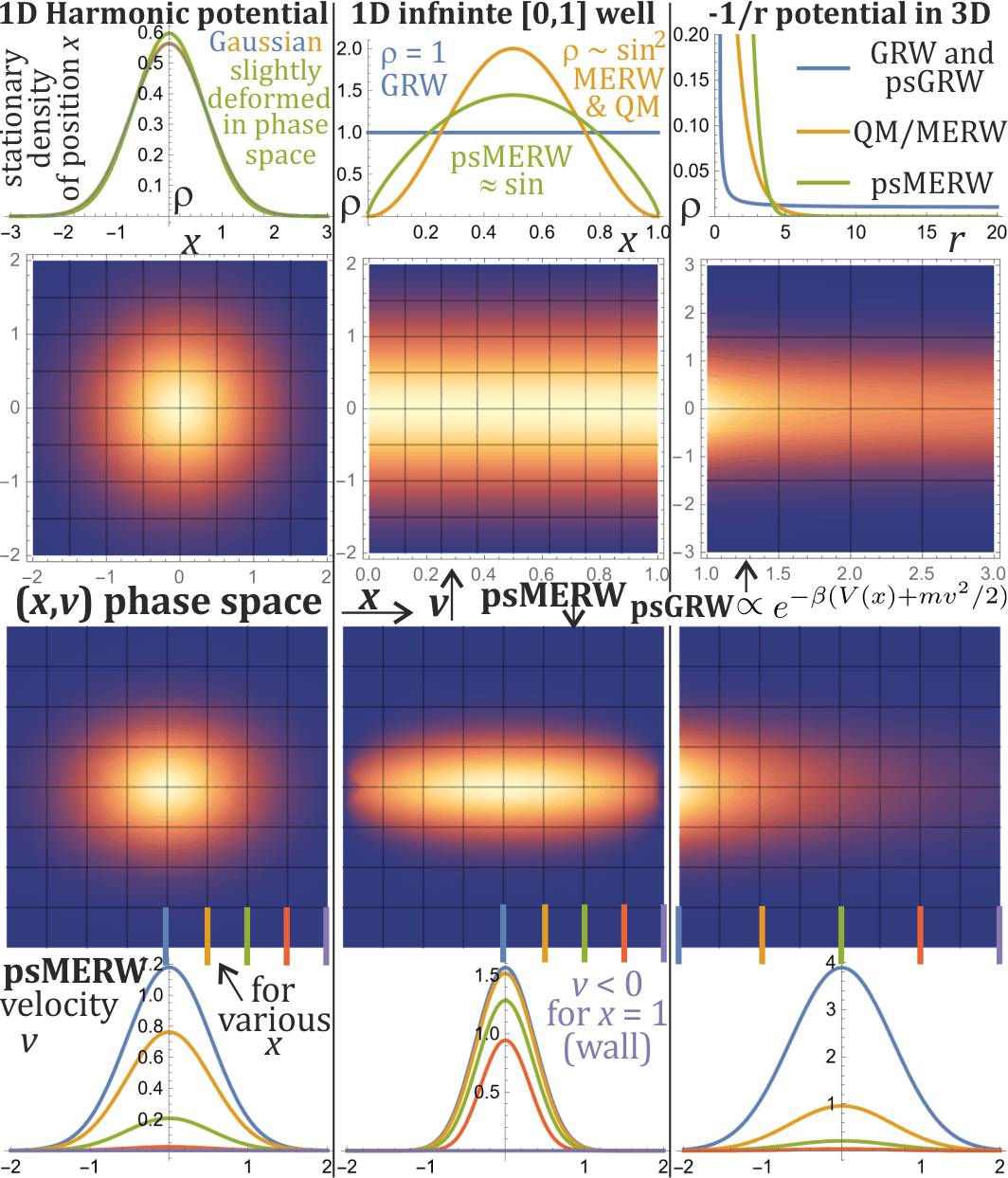
Figure 1: Examples of 4 types of predictions for 3 basic scenarios: 1D harmonic potential, 1D infinite well, and radial 3D $V\propto-1/r$ point electric or gravitational potential. Top: predicted $\rho(x)$ spatial stationary probability densities - for GRW and psGRW it is Boltzmann distribution in space. For MERW and QM it is Boltzmann path ensemble in space: $\rho\propto\psi^{2}$ for satisfying (Schrödinger) eigenequation $E\psi(x)=(-\Delta_{x}+V(x))$ for minimal energy $E$. For proposed psMERW it is Boltzmann path ensemble in phase space - as for MERW but for $E\psi(x,v)=(-\Delta_{v}-4v\cdot\nabla_{x}+V(x)+\|v\|^{2})\,\psi(x,v)$ eigenequation with $\rho(x,v)\propto\psi(x,v)\,\psi(x,-v)$ (here found with Wolfram Mathematica ”NDEigensystem”). Center: stationary probability density in phase space for psGRW (upper) and psMERW (lower). Below are its chosen cross-sections for positions shown with colors. MERW has stationary probability distribution exactly as quantum ground state, e.g. $\rho\propto\sin^{2}$ for infinite potential well, we can see psMERW predictions are slightly deformed, what might be experimentally distinguishable, e.g. $\rho=\,$const vs $\propto\sin$ vs $\sin^{2}$ near barriers.

To consider ensembles of more physical trajectories, as in Langevin equation [2] we can go to $(x,v)$ phase space - include finite velocity $v$ in evolved state, which evolves randomly and controls evolution in space $(x_{t+1}-x_{t}\propto v_{t})$. To get various behaviors which could be compared experimentally, there is included general spatial potential $V(x)$.

Another basic crucial question is if we should base on maximizing local entropy production GRW (generic random walk) with walker considering single steps, what leads to Boltzmann ensemble in space. Or maybe better use maximizing mean entropy production MERW (maximal entropy random walk) using Boltzmann ensemble of entire paths - like random walk along Ising sequence, or ”Wick-rotated” Feynman path ensembles, Euclidean quantum mechanics [3] - mathematically leading to the same stationary probability distribution as quantum ground state, with much stronger Anderson-like localization property [4].

This much stronger QM/MERW localization is crucial especially for electrons in semiconductor - standard diffusion would predict nearly uniform stationary electron probability distribution for such lattice of usually two types of atoms, which should flow if attaching external potential. In contrast, in QM/MERW and experiments these electrons are strongly localized, visualized e.g. in [5], what prevents conductance in such semiconductor. MERW allows for working diffusions model of e.g. diode as semiconductor p-n junction [6].

Neutrons are another objects confirmed to have quantum ground state stationary probability distribution [7] as predicted by both MERW and QM. Also for ”walking droplets”: classical objects with wave-particle duality, there were experimentally observed QM-like statistics [8]. They brings a difficult general question which approach should be used in which case, e.g. for diffusion of molecules, solitons, or dust halos in astronomical settings.

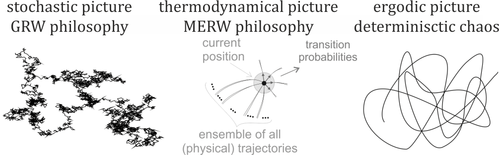
Figure 2: Three basic philosophies to predict stationary probability distributions. Left: in stochastic picture we basically guess stochastic propagator, usually maximizing entropy separately for each step (GRW), what leads to Boltzmann ensemble of positions in space. Right: in ergodic picture we assume we fully control deterministic evolution. Center: in contrast, in thermodynamics, statistical physics we do not assume knowing such details. Instead, we assume the safest statistical model accordingly to Jaynes’ principle: maximizing entropy. It leads to: for each point consider Boltzmann ensemble of possible paths from it, their statics give MERW stochastic propagator. It is nonlocal (depends on the entire situation), but effective model - used only by us to predict the most likely distributions, not used by the object itself - governed by some complex unknown evolution. In this article we expand MERW philosophy to phase space, using Boltzmann ensemble of more physical trajectories.

While MERW might be appropriate for frequently interacting objects, e.g. for rarely interacting sparse dust halo it seems more connivent to consider MERW in phase space. Combining them was one of motivations for this article, also to compare predictions of all these models, which hopefully could be experimentally distinguished in some future.

Beside Langevin equation, related approaches are e.g. phase-space formulation of quantum mechanics [9], or Feynman path ensemble in phase space [10]. However, they do not actually use velocities to choose spatial step, leading to different equations. While here we consider Boltzmann path ensembles in phase space, for Feynman it can be found in [11] discussed further.

Unfortunately formulas for such more physical trajectories become more complicated, requiring to solve functional eigenequations, for which analytical solutions could be found rather only for very simple cases. Fortunately there are available tools to do it numerically, like the used NDEigensystem function of Wolfram Mathematica.

Section II introduces to GRW and MERW philosophies including continuous limit. Section III contains their proposed extension to phase space. This is early version of article, hopefully stimulating further research in this direction, especially toward experimental distinguishing of the discussed 4 approaches.

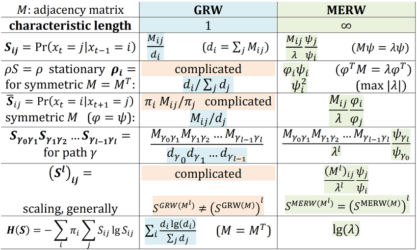
Figure 3: Gathered GRW, MERW formulas for graph defined by matrix $M$.

II Generic and maximal entropy random walk

This section briefly introduces to GRW/MERW random walks summarized in Fig. 2, 3, for details see e.g. [4, 12].

While further we will use lattice for continuous limit, let us start with general random walk on a graph given by adjacency matrix $M$: $M_{ij}=0$ if there is no edge between $i$ and $j$, otherwise it is 1, or for generality it has some weight here. For Boltzmann path ensemble it is natural to parameterize:

$$M_{ij}=\exp(-\beta V_{ij})\qquad(\textrm{e.g.}\ V_{ij}=(V_{i}+V_{j})/2)$$ (1)

for $V_{ij}$ being energy of $i\to j$ step, and $\beta=1/k_{B}T$ in thermodynamics for $T$ temperature, for quantum-like statistics can be related with Planck’s $\hbar$.

For such given $M$ matrix we would like to find stochastic matrix of transition probabilities for Markov process:

$$S_{ij}=\textrm{Pr}(X_{t}=j|X_{t-1}=i)\quad\textrm{satisfying}\quad\sum_{j}S_{ij}=1$$

and using only allowed transitions: $M_{ij}=0\Rightarrow S_{ij}=0$, what is equivalent with assigning $V_{ij}=\infty$ energy to this transition.

A basic approach to choose $S$, referred as generic random walk (GRW), is assuming uniform/Boltzmann ensemble among single possible steps, this way maximizing local entropy for this step (minus mean energy for Boltzmann):

$$S^{GRM}_{ij}=\frac{M_{ij}}{d_{i}}\quad\textrm{for}\quad d_{i}=\sum_{j}M_{ij}$$ (2)

For symmetric $M=M^{T}$ it leads to stationary probability distribution $\rho S=\rho$ being just $\rho_{i}^{GRW}=d_{i}/\sum_{j}d_{j}$.

II-A Maximal entropy random walk (MERW)

In contrast, in MERW we maximize mean entropy production (minus mean energy for Boltzmann), what is equivalent to uniform/Boltzmann ensemble among infinite paths.

The basic tool to calculate its stationary distribution and propagator is noticing that for $M_{ij}=\exp(-\beta V_{ij})$, matrix power $M^{l}$ combinatorially contains sum of Boltzmann path ensemble:

$$(M^{l})_{ij}=\sum_{\gamma:\gamma_{0}=i,\gamma_{l}=j}\exp(-\beta E(\gamma))\qquad\textrm{for}\ \ E(\gamma)=\sum_{i=1}^{l}V_{\gamma_{i-1}\gamma_{i}}$$ (3)

We are interested in $l\to\infty$ limit, for which using natural assumption of connected and acyclic graph, the Frobenius-Perron theorem says there is a single dominant eigenvalue $\lambda$, allowing to use $\phi,\psi$ dominant eigenvectors in the limit:

$$M^{l}\propto\lambda^{l}\psi\phi^{T}\equiv\lambda^{l}|\psi\rangle\langle\phi|\qquad\textrm{for}\quad l\to\infty$$ (4)

$$M\psi=\lambda\psi\qquad\phi^{T}M=\lambda\phi^{T}\quad\textrm{maximizing}\ |\lambda|$$

We can use both (3) and (4) to find propagator and stationary probability distribution (for any $j,k$) as in Fig. 4:

$$S_{ij}^{MERW}=\frac{\textrm{Pr}(ij)}{\textrm{Pr}(i)}=\lim_{l\to\infty}\frac{M_{ij}(M^{l})_{jk}}{(M^{l+1})_{ik}}=\frac{M_{ij}}{\lambda}\frac{\psi_{j}}{\psi_{i}}$$ (5)

$$\rho^{MERW}_{i}\propto\lim_{\l\to\infty}(M^{l})_{ji}(M^{l})_{ik}\propto\phi_{i}\psi_{i}$$ (6)

This way $\phi$ is distribution at the end of past half-paths, $\psi$ at the end of future half-paths. They come from $M^{l}$ or $(M^{T})^{l}$ for $l\to\infty$ propagators from minus/plus infinity, differing by time direction. To get some position we need to randomly get it from both direction, so its probability is $\rho_{i}\propto\phi_{i}\psi_{i}$ product of two probabilities. For (time) symmetric $M=M^{T}$ both eigenvectors are equal: $\phi=\psi$, getting $\rho_{i}\propto\psi_{i}^{2}$ Born rule.

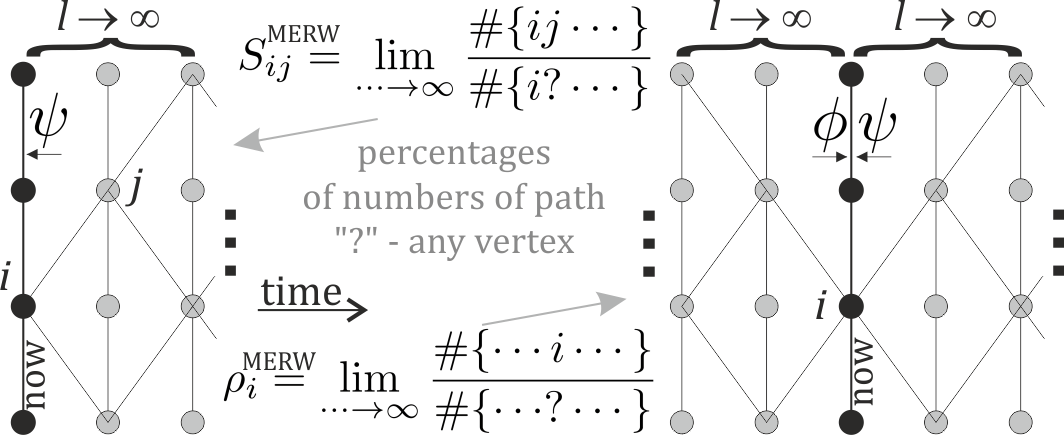
Figure 4: Diagrams for derivation of MERW formulas from path ensembles, exploiting that for $M_{ij}=\exp(-\beta V_{ij})$, matrix power $(M^{l})_{ij}\approx\lambda^{l}\psi\phi^{T}$ combinatorially contains summation over uniform/Boltzmann ensemble of length $l$ paths from $i$ to $j$. To get stochastic propagator $S^{MERW}_{ij}$, we can consider length $l$ paths from vertex $i$, and look at distribution of their first step for $l\to\infty$ limit. To get stationary probability distribution we can multiply such two propagators: $\rho_{i}\propto\lim_{l\to\infty}(M^{l})_{ji}(M^{l})_{ik}\propto\phi_{i}\psi_{i}$.

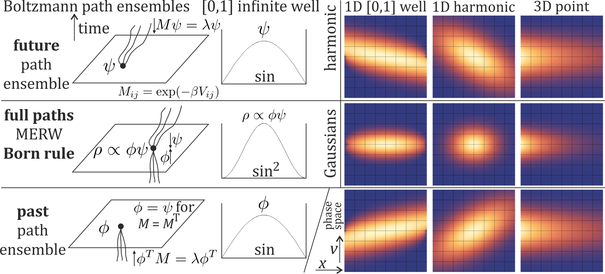
Figure 5: Boltzmann path ensembles: $\psi$ is probability distribution at the end of future half-paths, $\phi$ at the end of past half-paths. They can be viewed as results of propagator from plus/minus infinity: $M^{l}$, $(M^{T})^{l}$ for $l\to\infty$. To get stationary probability distribution in the center of full paths we need to randomly get it from both directions: $\rho=\phi\psi$ Born rule. While for (time) symmetric $M=M^{T}$ both are equal $\phi=\psi$, in the discussed phase space case, time symmetry inverses velocity - on the right there are 3 cases as in Fig. 1, now with shown $\psi(x,v)=\phi(x,-v)$, which differ by inversion of velocity, making $\rho=\phi\psi$ symmetric. This symmetry is required as inverting all paths in their Feynman ensemble (including velocities), we get the same ensemble. While here for Boltzmann path ensembles we need two real eigenfunctions, in Feynman path ensembles they are combined in real/imaginary parts of single complex eigenfunction [11].

II-B Lattice and MERW continuous limit to Schrödinger equation

Let us discretize space $\mathbb{R}^{D}\ni x=\delta\tilde{x}$ for $\tilde{x}\in\mathbb{Z}^{D}$ and time $\mathbb{R}\ni t=\epsilon\tilde{t}$ for $\tilde{t}\in\mathbb{Z}$. For continuous limit $\epsilon,\delta\to 0$. Also discretize spatial potential: $V_{\tilde{x}}\equiv V(\delta\tilde{x})$. For simplicity let us work in $D=1$, with mentioned generalization for $D>1$.

II-B1 GRW leading to Boltzmann space ensemble

Allowing only jumps up to the nearest neighbors: step $s\in\{-1,0,1\}$, we can choose $M$ matrix as symmetric and using potential:

$$M_{\tilde{x},\tilde{x}+s}=\exp(-\beta(V_{\tilde{x}}+V_{\tilde{x}+s})/2)\quad\textrm{for }s\in\{-1,0,1\}$$ (7)

as it is symmetric, GRW stationary probability distribution is $\rho_{\tilde{x}}\propto M_{\tilde{x},\tilde{x}-1}+M_{\tilde{x},\tilde{x}}+M_{\tilde{x},\tilde{x}+1}$. Assuming continuous potential $V(x)$, in the limit we get just Boltzmann ensemble in space:

$$\rho^{GRW}(x)\propto\exp(-\beta V(x))$$ (8)

II-B2 MERW leading to Schrödinger ground state

For MERW we assume Boltzmann ensemble among paths, with path energy as sum of energies of single transitions. For continuous limit this energy should become integral over time $E(\gamma)=\int V(\gamma(t))dt$, what requires to include time step $\epsilon$ in transition energy:

$$M_{\tilde{x},\tilde{x}+s}=\exp(-\beta\epsilon((V_{\tilde{x}}+V_{\tilde{x}+s})/2)$$

For MERW we first need to find the dominant eigenvector of adjacency matrix $\lambda\psi=M\psi$ for $M$ given by (7):

$$\lambda\psi_{\tilde{x}}=(M\psi)_{\tilde{x}}=\sum_{s\in\{-1,0,1\}}e^{-\beta\epsilon(V_{\tilde{x}}+V_{\tilde{x}+s})/2}\ \psi_{\tilde{x}+s}$$ (9)

Taking $\exp(-\epsilon)\approx 1-\epsilon$ first order expansion and assuming continuous potential $V(x)$, for continuous limit we can approximate the above with:

$$\lambda\psi_{\tilde{x}}\approx\psi_{\tilde{x}-1}+\psi_{\tilde{x}}+\psi_{\tilde{x}+1}-3\beta\epsilon V_{\tilde{x}}$$

Subtracting $3\psi_{\tilde{x}}$ from both sides, and multiplying by $-1/3\beta\epsilon$:

$$\frac{3-\lambda}{3\beta\epsilon}\psi_{\tilde{x}}\approx-\frac{1}{3\beta}\frac{\psi_{\tilde{x}-1}-2\psi_{\tilde{x}}+\psi_{\tilde{x}+1}}{\epsilon}+V_{\tilde{x}}\psi_{\tilde{x}}$$

Due to change of sign, maximization of eigenvalue $|\lambda|$ becomes minimization of $(3-\lambda)/(3\beta\epsilon)$, which in continuous limit should converge to some energy $E$. Assuming $\epsilon=\delta^{2}$, the difference term will lead to Laplacian, hence in continuous limit we can write the eigenequation as stationary Schrödinger equitation searching for the lowest energy $E$ ground state:

$$E\psi=-C\Delta\psi+V\psi\qquad\quad\rho^{MERW}(x)\propto(\psi(x))^{2}$$ (10)

for $C=1/3\beta$ in 1D or generally $1/(2D+1)$ in dimension $D$. We can choose parameters to make it $C=\hbar^{2}/2m$ as in standard Schrödinger equitation, what is explored e.g. in  [12] or in [13] finding also some agreement toward Dirac equation.

III Random walks in phase space

While standard random walks or Feynman path ensembles use nowhere differentiable paths of infinite kinetic energy, here we would like use more physical paths by going to phase space $(x,v)$: with random change of (finite) velocity $v$, which defines deterministic change of position $x$.

Like in popular Langevin approach [2]:

$$m\frac{dx}{dt}=v\qquad\qquad m\frac{dv}{dt}=-\Gamma v+\eta$$

for $\Gamma$ describing damping (neglected in current version). It has no potential, hence independent finite variance infinitesimal steps would lead to Gaussian distribution for velocities.

Here we would like to include energy - both kinetic $mv^{2}/2$ and some general position dependant $V(x)$:

$$\bar{V}(x,v)=V(x)+m\|v\|^{2}/2$$ (11)

III-A GRW phase space continuous limit (psGRW)

Discretizing $\mathbb{Z}\ni\tilde{x}=x/\delta$ position, and $\mathbb{Z}\ni\tilde{v}=v/\zeta$ velocity, GRW as Boltzmann ensemble of single steps e.g. $s,s^{\prime}\in\{-1,0,1\}$ can be chosen as:

$$S_{(\tilde{x},\tilde{v}),(\tilde{x}+\tilde{v},\tilde{v}+s)}=\frac{\exp(-\beta(V(\delta\tilde{x})+\frac{1}{2}m(\zeta(\tilde{v}+s))^{2}))}{\sum_{s^{\prime}}\exp(-\beta(V(\delta\tilde{x})+\frac{1}{2}m(\zeta(\tilde{v}+s^{\prime}))^{2}))}$$

The spatial potential contributions $V(\delta\tilde{x})$ cancel out - leaving random walk of velocity alone, in $mv^{2}/2$ kinetic energy acting as harmonic potential for velocity.

Therefore, while $M$ is not symmetric due to velocity inversion in $M^{T}$, for velocity alone it can be made symmetric, leading to $\rho(v)\propto\exp(-\beta mv^{2}/2)$ Gaussian stationary probability distribution for velocity, independent from position.

For such position independent symmetric Gaussian velocity distributions, in infinitesimal limit we can get symmetric $M$ among positions, allowing to conclude psGRW stationary probability distributions as Boltzmann distribution in the phase space:

$$\rho^{psGRW}(x,v)\propto\exp(-\beta(V(x)+mv^{2}/2))\rho$$ (12)

III-B MERW phase space continuous limit (psMERW)

III-B1 Derivation

Let us discretize space $\mathbb{R}^{D}\ni x=\delta\tilde{x}$ for $\tilde{x}\in\mathbb{Z}^{D}$ and time $\mathbb{R}\ni t=\epsilon\tilde{t}$ for $\tilde{t}\in\mathbb{Z}$. For continuous limit we will take $\epsilon,\delta\to 0$. Discretized $\tilde{v}\in\mathbb{Z}^{D}$ velocity for $\tilde{x}\to\tilde{x}+\tilde{v}$ transition in single step corresponds to $v=\frac{\delta}{\epsilon}\tilde{v}\in\mathbb{R}^{D}$ real velocity. As previously we calculate for $D=1$, then mention for general $D$.

Denote $\psi_{\tilde{x},\tilde{v}}=\psi(\delta\tilde{x},\frac{\delta}{\epsilon}\tilde{v})=\psi(x,v)$ as discretization of continuous eigenfunction in phase space. Analogously for potential: $\bar{V}_{\tilde{x},\tilde{v}}=\bar{V}(\delta\tilde{x},\frac{\delta}{\epsilon}\tilde{v})=\bar{V}(x,v)$.

In one step $\tilde{x}\to\tilde{x}+\tilde{v}$, and there is a random velocity change $\tilde{v}\to\tilde{v}+s$, we can assume $s\in\{-1,0,1\}$. To include damping in future, we could add velocity reduction in below step. In 1D the MERW eigenequation after neglecting $O(\epsilon^{2})$ terms becomes:

$$\lambda\psi_{\tilde{x},\tilde{v}}=(M\psi)_{\tilde{x},\tilde{v}}=\sum_{s\in\{-1,0,1\}}e^{-\epsilon\beta\bar{V}_{\tilde{x}+\tilde{v},\tilde{v}+s}}\psi_{\tilde{x}+\tilde{v},\tilde{v}+s}\approx$$ (13)

$$\approx\sum_{s\in\{-1,0,1\}}(1-\epsilon\beta\bar{V}_{\tilde{x},\tilde{v}})(\psi_{\tilde{x},\tilde{v}+s}+\epsilon v(\nabla_{x}\psi)_{\tilde{x},\tilde{v}})$$

thanks to approximation with derivative $\nabla_{x}\equiv\partial/\partial x$:

$$\psi_{\tilde{x}+\tilde{v},\tilde{v}}=\psi(\delta(\tilde{x}+\tilde{v}),v)=\psi(x+\epsilon v,v)\approx\psi_{\tilde{x},\tilde{v}}+\epsilon v(\nabla_{x}\psi)_{\tilde{x},\tilde{v}}$$

Neglecting $O(\epsilon^{2})$ terms eigenequation (13) becomes:

$$\lambda\psi_{\tilde{x},\tilde{v}}\approx\psi_{\tilde{x},\tilde{v}-1}+\psi_{\tilde{x},\tilde{v}}+\psi_{\tilde{x},\tilde{v}+1}+3\epsilon v(\nabla_{x}\psi)_{\tilde{x},\tilde{v}}-3\beta\epsilon\bar{V}_{\tilde{x},\tilde{v}}\psi_{\tilde{x},\tilde{v}}$$

Now subtract $3\psi_{\tilde{x},\tilde{v}}$ from both sides and multiply by $-1/(3\beta(\delta/\epsilon)^{2})$, getting:

$$\frac{3-\lambda}{3\beta(\delta/\epsilon)^{2}}\psi_{\tilde{x},\tilde{v}}\approx-\frac{1}{3\beta}\frac{\psi_{\tilde{x},\tilde{v}-1}-2\psi_{\tilde{x},\tilde{v}}+\psi_{\tilde{x},\tilde{v}+1}}{(\delta/\epsilon)^{2}}-$$

$$-v\frac{1}{\beta}\frac{\epsilon}{(\delta/\epsilon)^{2}}(\nabla_{x}\psi)_{\tilde{x},\tilde{v}}+\frac{\epsilon}{(\delta/\epsilon)^{2}}\bar{V}_{\tilde{x},\tilde{v}}\psi_{\tilde{x},\tilde{v}}$$

Assuming $\delta/\epsilon\to 0$, the discrete Laplacian tends to continuous $\Delta_{v}$ for velocity. As previously we would like to interpret the first coefficient as energy: $\frac{3-\lambda}{3\beta(\delta/\epsilon)^{2}}\to E$.

For $\nabla_{x}$ gradient term we can choose:

$$\frac{1}{\beta}\frac{\epsilon}{(\delta/\epsilon)^{2}}\to\xi\qquad\textrm{for example}\quad\epsilon=\sqrt[3]{\beta\xi\,\delta^{2}}$$ (14)

or use a sequence $\xi\to 0$ for $\xi=0$ in continuous case.

Finally in the continuous limit we get stationary phase space Schrödinger equation for $\psi\equiv\psi(x,v)$:

$$E\psi=-C\Delta_{v}\psi-\xi v\cdot\nabla_{x}\psi+\left(V+\frac{1}{2}m\|v\|^{2}\right)\psi$$ (15)

where $C=\frac{1}{3\beta}$, or generally $C=\frac{1}{(2D+1)\beta}$ in dimension $D$, is some constant which can be directly chosen, e.g. dependent on $\hbar$ or temperature. Analogously for $\xi$, down to $\xi\to 0$ limit making position and velocity independent.

To find the stationary probability distribution $\rho(x,v)$, we need to solve eigenequation (15) minimizing energy $E$, what corresponds to $|\lambda|$ maximization. Higher energy contributions have exponential decay here. This time $M$ is not symmetric as $M^{T}$ time symmetry inverses velocity, so we should find left/right eigenfunction. Fortunately, as in Fig. 5, they differ by just change of sign of velocity $\phi(x,v)=\psi(x,-v)$, getting Born rule:

$$\rho(x,v)\propto\psi(x,v)\ \psi(x,-v)$$ (16)

III-B2 Comparison with Feynman path ensemble

Similar $t\to it$ ”Wick rotated” phase space Schrödinger equation was earlier derived by Bouchaud [11] for QM, Feynman path ensembles:

$$i\hbar\frac{\partial\Psi(x,q)}{\partial t}=\frac{\hbar}{2\tau_{c}}[\Delta_{q}\Psi(x,q)-q^{2}\Psi(x,q)]+$$

$$\qquad+i\sqrt{\frac{\hbar^{3}}{m\tau_{c}}}q\nabla_{x}\Psi(x,q)+V(x)\Psi(x,q)$$ (17)

for $\tau_{c}$ momentum correlation time: as in Ornstein-Uhlenbeck process assuming $\langle p(s)p(u)\rangle=\frac{m\hbar}{2\tau_{c}}\exp(-|s-u|/\tau_{c})$, and rescaled momentum $p=\sqrt{m\hbar/\tau_{c}}q$. Comparing it with (15) suggests parameter choice for quantum scale applications.

Beside $t\to it$ ”Wick rotation to imaginary time”, there are some subtle differences between Boltzmann and Feynman path ensembles. Hamiltonian corresponds to minus $M$ matrix, energy $E$ corresponds to minus $\lambda$ - discussed here maximization of $\lambda$ corresponds to minimization of energy for the ground state.

In Boltzmann path ensemble excited states vanish exponentially: $M\psi^{k}=\lambda_{k}\psi^{k}$ for $|\lambda_{0}|\geq|\lambda_{1}|\geq\ldots$, then after $t$ steps $\sum_{k}a_{k}\psi^{k}\to\sum_{k}(\lambda_{k}/\lambda_{0})^{t}a_{k}\psi^{k}$. In contrast, in QM/Feynman path ensembles $\psi^{k}$ excited states are stable, rotate in complex plane. Excited e.g. atoms are believed to deexcite through interaction with environment.

Transposition $M^{T}$ corresponds to time reversal. As in Fig. 5, for non-symmetric $M$ ensembles of future and past half-paths lead to different $\phi,\psi$ which are real for Boltzmann ensembles. In contrast, (17) Hamiltonian is self-adjoint: invariant under time symmetry in conjugation, containing such two asymmetric real eigenfunction in real/imaginary parts of one complex wavefunction.

III-B3 Calculation remarks

While for QM/MERW there are well known analytical solutions of such stationary Schrödinger equation e.g. for harmonic potential, infinite well, point $V\propto-1/r$ potential, their phase space version are more complicated and Wolfram Mathematica DEigensystem was not able to find analytical solutions, hence for their example solution in Fig. 1 there was used numerical NDEigensystem, also required for more complex settings.

Function NDEigensystem uses finite element method, and already had various issues in the discussed basic cases - resolved e.g. by manually specifying Dirchlet conditions for infinite well, or for point potential: solving for $\psi(x,v)\sim\exp(-v^{2}-x)\phi(x,v)$ type substitution assuming asymptotic behavior. Alternative approach is approximation by solving in a finite orthogonal basis of functions (removing higher modes), especially Gaussian distribution times Hermite polynomial for velocities (ground state already gets such higher modes), further developed in [11]. Numerical methods for psMERW will require further work, especially to include interaction between multiple particles.

IV Conclusions and further work

While popularly considered path ensembles usually use infinite kinetic energy paths, it is mathematically more difficult but doable to use ensembles of more physical paths instead by going to phase space. This article discusses some basics with included spatial potential to bring attention, hopefully leading to some attempts to experimentally determine the most appropriate ones for various physical settings.

This is early article opening various directions for further work, e.g.:

• Search for possibilities of experimental determination which of the discussed approaches is the most appropriate, especially using stationary probability distributions of positions, maybe also velocities e.g. from redshifts - in various settings from microscopic e.g. neutrons [7], molecules, solitons [8], to astronomical e.g. dust halos.

• Find parameters, understand their dependence, universality.

• Mathematical improvements, especially of numerical approaches, also search for analytical formulas for basic cases, maybe include damping like in Langevin equation, include larger velocity changes through collisions, include relativistic corrections, etc.

• While for simplicity we have discussed only stationary situation, it seems worth to also consider dynamics - both straightforward evolution in fixed potential like for electron conductance [6], but also much more difficult case of varying potential - with basics discussed in [12].

• While the discussed analysis was for a single walker, in practice we usually have multiple interacting - what should be finally included. One way is through mean-field treatment assuming the remaining have the same distribution, used e.g. for MERW electron conductance model [6] to include potential contributions from the remaining electrons. For psMERW it could be useful e.g. for astronomical dust halos to include their gravitational self-interaction.

• While we have focused on ensembles of full trajectories, maybe it is also valuable to consider unidirectional, which have asymmetric velocity distributions like in Fig. 5.

• While we have focused on continuous limit of infinitesimal lattice constants, finite lattice can be considered e.g. for conductance models imagining electrons jumping between atoms in a lattice. Also, for MERW Darwin term was recently derived [13] as correction from use of finite lattice. Especially the latter suggests to also consider psMERW in some finite lattice, and closely look at corrections it brings.

References

- [1] R. P. Feynman, “Space-time approach to non-relativistic quantum mechanics,” Reviews of Modern Physics, vol. 20, no. 2, p. 367, 1948.
- [2] P. Langevin, “Sur la théorie du mouvement brownien,” Compt. Rendus, vol. 146, pp. 530–533, 1908.
- [3] J. Zambrini, “Euclidean quantum mechanics,” Physical Review A, vol. 35, no. 9, p. 3631, 1987.
- [4] Z. Burda, J. Duda, J.-M. Luck, and B. Waclaw, “Localization of the maximal entropy random walk,” Physical review letters, vol. 102, no. 16, p. 160602, 2009.
- [5] A. Richardella, P. Roushan, S. Mack, B. Zhou, D. A. Huse, D. D. Awschalom, and A. Yazdani, “Visualizing critical correlations near the metal-insulator transition in Ga1-xMnxAs,” science, vol. 327, no. 5966, pp. 665–669, 2010.
- [6] J. Duda, “Diffusion models for atomic scale electron currents in semiconductor, pn junction,” arXiv preprint arXiv:2112.12557, 2021.
- [7] V. V. Nesvizhevsky, H. G. Börner, A. K. Petukhov, H. Abele, S. Baeßler, F. J. Rueß, T. Stöferle, A. Westphal, A. M. Gagarski, G. A. Petrov et al., “Quantum states of neutrons in the earth’s gravitational field,” Nature, vol. 415, no. 6869, pp. 297–299, 2002.
- [8] D. M. Harris, J. Moukhtar, E. Fort, Y. Couder, and J. W. Bush, “Wavelike statistics from pilot-wave dynamics in a circular corral,” Physical Review E, vol. 88, no. 1, p. 011001, 2013.
- [9] H. J. Groenewold and H. J. Groenewold, On the principles of elementary quantum mechanics. Springer, 1946.
- [10] F. A. Berezin, “Feynman path integrals in a phase space,” Soviet Physics Uspekhi, vol. 23, no. 11, p. 763, 1980.
- [11] J.-P. Bouchaud, “Quantum mechanics with a nonzero quantum correlation time,” Physical Review A, vol. 96, no. 5, p. 052116, 2017.
- [12] J. Duda, “Extended maximal entropy random walk,” Ph.D. dissertation, Jagiellonian University, 2012. [Online]. Available: http://www.fais.uj.edu.pl/documents/41628/d63bc0b7-cb71-4eba-8a5a-d974256fd065
- [13] M. Faber, “Stationary schrodinger equation and darwin term from maximal entropy random walk,” Particles, vol. 7, no. 1, pp. 25–39, 2024, preprint: https://arxiv.org/abs/2304.02368.