Unique Ergodicity of Stochastic Theta Method for Monotone SDEs driven by Nondegenerate Multiplicative Noise

Abstract.

We establish the unique ergodicity of the Markov chain generated by the stochastic theta method (STM) with $\theta\in[1/2,1]$ for monotone SODEs, without growth restriction on the coefficients, driven by nondegenerate multiplicative noise. The main ingredient of the arguments lies in the construction of new Lyapunov functions, involving the coefficients, the stepsize, and $\theta$, and the irreducibility and the strong Feller property for the STM. We also generalize the arguments to the STM and its Galerkin-based full discretizations for a class of monotone SPDEs driven by infinite-dimensional nondegenerate multiplicative trace-class noise. Applying these results to the stochastic Allen–Cahn equation indicates that its drift-implicit Euler scheme is uniquely ergodic for any interface thickness, which gives an affirmative answer to a question proposed in (J. Cui, J. Hong, and L. Sun, Stochastic Process. Appl. (2021): 55–93). Numerical experiments verify our theoretical results.

1. Introduction

The long-time behavior of Markov processes generated by stochastic differential equations (SDEs) is a natural and intriguing question and has been investigated in the recent decades. As a significant long-time behavior, the ergodicity characterizes the case of temporal average coinciding with spatial average, which has a lot applications in quantum mechanics, fluid dynamics, financial mathematics, and many other fields [12, 17]. The spatial average, i.e., the mean of a given test function for the invariant measure of the considered Markov process, also known as the ergodic limit, is desirable to compute in practical applications, then one has to investigate a stochastic system over long-time intervals, which is one of the main difficulties from the computational perspective. It is well-known that the explicit expression of the invariant measure for a stochastic nonlinear system is rarely available; exceptional examples are gradient Langevin systems driven by additive noise, see, e.g., [3, 20]. For this reason, it motivates and fascinates a lot of investigations in the recent decade for constructing numerical algorithms that can inherit the ergodicity of the original system and approximate the ergodic limit efficiently.

Much progress has been made in the design and analysis of numerical approximations of the desired ergodic limits for SDEs under a strong dissipative condition so that the Markov chains are contractive, see, e.g., [22, 33] and references therein for numerical ergodicity of backward Euler or Milstein schemes for dissipative SODEs, [21] for dissipative SODEs with Markovian switching, and [4, 5, 7, 8, 9, 11, 24] for approximating the invariant measures via temporal tamed, Galerkin-based linearity-implicit Euler or exponential Euler schemes, and high order integrator for parabolic SPDEs driven by additive noise. See also [28] and [15] for numerical ergodicity of backward Euler scheme and its versions for monotone SODEs and spectral Galerkin approximation for 2-dimensional stochastic Navier–Stokes equations, respectively, both driven by additive degenerate noise.

We note that most of the above works of literature focus on the numerical ergodicity of SDEs driven by additive noise, the numerical ergodicity in the multiplicative noise case is more subtle and challenging. On the other hand, the authors in [11] investigated the temporal drift-implicit Euler (DIE) spectral Galerkin scheme to approximate the invariant measure of the stochastic Allen–Cahn equation and proposed a question of whether the invariant measure of the DIE scheme is unique.

The above two questions on the unique ergodicity of numerical approximations for monotone SDEs in both finite-dimensional and infinite-dimensional settings motivate the present study. Our main aim is to establish the unique ergodicity of the STM (see (STM) with $\theta\in[1/2,1]$), including the numerical schemes studied in [16, 28, 31] for monotone SODEs, without growth restriction on the coefficients, driven by nondegenerate multiplicative noise. The main ingredient of our arguments lies in the construction of a new Lyapunov function, in combination with the irreducibility and the strong Feller property for the STM.

It is not difficult to show that $V(\cdot)=\left\lvert\cdot\right\rvert^{2}$ is a natural Lyapunov function of the considered monotone (SDE). However, it was shown in [18] that the Euler–Maruyama scheme (i.e., (STM) with $\theta=0$) applied to Eq. (SDE) with superlinear growth coefficients would blow up in $p$-th moment for all $p\geq 2$. Therefore, $\left\lvert\cdot\right\rvert^{2}$ is not an appropriate Lyapunov function of this scheme in the setting of the present study, and we mainly focus on the case $\theta\in[1/2,1]$. By exploring the monotone structure of the coefficients and martingale property of the driven Wiener process, we construct several Lyapunov functions (see, e.g., (3.2) and (3.6)) for the STM, which involves both the coefficients, the stepsize, and $\theta$.

Then we generalize our methodology to the temporal DIE scheme (see STM (4.15) with $\theta=1$), and its Galerkin-based fully discrete schemes (see (DIEG)), including the numerical schemes studied in [11, 14, 19, 25, 27] for monotone SPDEs, with polynomial growth coefficients, driven by infinite-dimensional nondegenerate multiplicative trace-class noise. Applying these results to the stochastic Allen–Cahn equation driven by nondegenerate noise indicates that the DIE scheme and its Galerkin-based full discretizations are uniquely ergodic, respectively, for any interface thickness, which gives an affirmative answer to the question proposed in [11].

The paper is organized as follows. In Section 2, we give the main assumptions on monotone SODEs and recall ergodic theory of Markov chains that will be used throughout. The Lyapunov structure of the STM, with irreducibility and strong Feller property, is explored in Section 3. In Section 4, we generalize the arguments in Section 3 to monotone SPDEs including the stochastic Allen–Cahn equation. The theoretical results are validated by numerical experiments in Section 5. We include some discussions in the last section.

2. Preliminaries

In this section, we present the required main assumptions and recall the general ergodic theory of Markov chains that will be used throughout the paper.

2.1. Main Assumptions

Let us first consider the $d$-dimensional SODE

(SDE) $$\mathrm{d}X(t)=b(X(t))\mathrm{d}t+\sigma(X(t))\mathrm{d}W(t),~{}t\geq 0,$$

driven by an $\mathbb{R}^{m}$-valued Wiener process $W$ on a complete filtered probability space $(\Omega,\mathscr{F},(\mathscr{F}(t))_{t\geq 0},\mathbb{P})$, where $b:\mathbb{R}^{n}\rightarrow\mathbb{R}^{n}$ and $\sigma:\mathbb{R}^{n}\rightarrow\mathbb{R}^{n\times m}$ are measurable functions.

Our main focus is on the invariant measure of the Markov chain generated by the following stochastic theta method (STM) with $\theta\in[0,1]$:

(STM) $$X_{j+1}=X_{j}+(1-\theta)b(X_{j})\tau+\theta b(X_{j+1})\tau+\sigma(X_{j})\delta_{j}W,$$

where $\tau\in(0,1)$ is a fixed step-size, $\delta_{j}W:=W(t_{j+1})-W(t_{j})$ with $t_{j}=j\tau$, $j\in\mathbb{N}$. When $\theta=0,1/2,1$, it is called the Euler–Maruyama scheme, the mid-point scheme, and the backward Euler method, respectively.

Our main conditions on the coefficients $b$ and $\sigma$ in Eq. (SDE) are the following coupled monotone and coecive conditions. Throughout we denote by $\left\lvert\cdot\right\rvert$ the Euclidean norm in $\mathbb{R}^{d}$ or $\mathbb{R}^{m}$, and by $\left\lVert\cdot\right\rVert$ the Hilbert–Schmidt norm in $\mathbb{R}^{d\times m}$.

Assumption 2.1.

There exists a constant $L_{1}\in\mathbb{R}$ such that

(2.1) $$2\left\langle b(x)-b(y),x-y\right\rangle+\left\lVert\sigma(x)-\sigma(y)\right\rVert^{2}\leq L_{1}\left\lvert x-y\right\rvert^{2},\quad\forall~{}x,y\in\mathbb{R}^{d}.$$

Under the monotone condition (2.1), one can show the existence and uniqueness of the $(\mathscr{F}_{t})_{t\geq 0}$-adapted solution to Eq. (SDE), see, e.g., [23, Theorem 3.1.1]. The following result gives the unique solvability of (STM).

Lemma 2.1.

Let Assumption 2.1 hold. The STM (STM) can be uniquely solved when $L_{1}\theta\tau<2$.

Proof.

Define

(2.2) $$\hat{b}(x)=x-\theta b(x)\tau,\quad x\in\mathbb{R}^{d}.$$

Then (STM) becomes

$$\hat{b}(X_{j+1})=X_{j}+(1-\theta)b(X_{j}^{h})\tau+\sigma(X_{j})\delta_{j}W,\quad j\in\mathbb{N}.$$

It follows from (2.1) that

$$\langle x-y,\hat{b}(x)-\hat{b}(y)\rangle =\left\langle x-y,x-y-(b(x)-b(y))\right\rangle\theta\tau$$

$$=\left\lVert x-y\right\rVert^{2}-\left\langle x-y,b(x)-b(y)\right\rangle{\color[rgb]{1,0,0}\theta}\tau$$

$$\geq(1-L_{1}\theta\tau/2)\left\lVert x-y\right\rVert^{2}.$$

As $L_{1}\theta\tau<2$, $\hat{b}$ defined in (2.2) is uniformly monotone so that it is invertible (see, e.g., [32, Theorem C.2]), from which we can conclude the unique solvability of (STM). ∎

Assumption 2.2.

There exist two positive constants $L_{2}$ and $L_{3}$ such that

(2.3) $$2\left\langle b(x),x\right\rangle+\left\lVert\sigma(x)\right\rVert^{2}\leq L_{2}-L_{3}\left\lvert x\right\rvert^{2},\quad\forall~{}x\in\mathbb{R}^{d}.$$

We also need the following non-degeneracy of $\sigma$.

Assumption 2.3.

For any $x\in\mathbb{R}^{d}$, $\sigma(x)\sigma(x)^{\top}$ is positive definite.

It is clear from Assumption 2.3 that the determinant $\det J_{b}(y)$ of the Jacobi matrix $J_{b}$ of $b$ is continuous.

Example 2.1.

A motivating example for $b$ and $\sigma$ satisfying Assumptions 2.1, 2.2, and 2.3 is

$$b(x)=x-x^{3},\quad\sigma(x)=\sqrt{x^{2}+1},\quad x\in\mathbb{R}.$$

Clearly, Assumption 2.3 holds. As $\sigma$ is Lipschitz continuous with Lipschitz constant 1, we have

$$\left\langle b(x)-b(y),x-y\right\rangle+\|\sigma(x)-\sigma(y)\|^{2}$$

$$=(x-y)^{2}(1-x^{2}-xy-y^{2})+|\sqrt{x^{2}+1}-\sqrt{y^{2}+1}|$$

$$\leq\left\lvert x-y\right\rvert^{2}(2-x^{2}-xy-y^{2})\leq 2\left\lvert x-y\right\rvert^{2},$$

$$2\left\langle b(x),x\right\rangle+\|\sigma(x)\|^{2}=2x^{2}-2x^{4}+x^{2}+1\leq 3-x^{2}.$$

as $x^{2}+xy+y^{2}\geq 0$, for all $x,y\in\mathbb{R}$. This shows Assumptions 2.1 and 2.2 with $L_{1}=2$ and $L_{2}=3$, $L_{3}=1$, respectively.

Under Assumptions 2.1, 2.2, and 2.3, Eq. (SDE) is ergodic, see, e.g., [34] for the use of coupling methods based on a changing measure technique in combination with Girsanov theorem. In discrete-time model, there does not exist such Girsanov theorem. Instead, we will ultilize general ergodic theory of Markov chains.

2.2. Preliminaries on Ergodicity of Markov Chains

Let $(H,\|\cdot\|)$ (either $\mathbb{R}^{d}$ in Section 3 and $L^{2}$-space in Section 4) be a separable Hilbert space equipped with Borel $\sigma$-algebra $\mathcal{B}(H)$. Let $(X_{n})_{n\in\mathbb{N}}$ be an $H$-valued Markov chain with transition kernel $P(x,B)$, $x\in H$, $B\in\mathcal{B}(H)$.

Recall that a set $C\in\mathcal{B}(H)$ is called an ($(m,\nu)$-)small set if there exists an integer $m>0$ and a non-trivial measure $\nu$ on $\mathcal{B}(H)$ such that

$$P^{m}(x,B)\geq\nu(B),\quad\forall~{}x\in C,~{}B\in\mathcal{B}(H).$$

$(X_{n})_{n\in\mathbb{N}}$ is said to satisfy the minorization condition (with $C$) if there exists some $\delta>0$, $C\in\mathcal{B}(H)$, and probability measure $\nu$ with $\nu(C)=1$ such that

(2.4) $$P(x,B)\geq\delta\chi_{C}(x)\nu(B),\quad\forall~{}x\in H,~{}B\in\mathcal{B}(H).$$

It is clear that if $(X_{n})_{n\in\mathbb{N}}$ satisfies the minorization condition (2.4) with $C$, then $C$ is a $(1,\delta\nu)$-small set. $(X_{n})_{n\in\mathbb{N}}$ is called (open set) irreducible if $P(x,A)>0$ for any $x\in H$ and open set $A$ in $H$; it is called strong Feller if $P(\cdot,A)$ is lower continuous for any Borel set $A\in\mathcal{B}(H)$. We refer to [29] for more details on Markov chains.

A probability measure $\mu$ on $H$ is called invariant for the Markov chain $(X_{n})_{n\in\mathbb{N}}$ or its transition kernel $P$, if

$$\int_{H}P\phi(x)\mu({\rm d}x)=\mu(\phi):=\int_{H}\phi(x)\mu({\rm d}x),\quad\forall~{}\phi\in\mathcal{C}_{b}(H).$$

This is equivalent to $\int_{H}P(x,A)\mu({\rm d}x)=\mu(A)$ for all $A\in\mathcal{B}(H).$ An invariant (probability) measure $\mu$ is called ergodic for $(X_{n})_{n\in\mathbb{N}}$ or $P$, if

(2.5) $$\lim_{m\to\infty}\frac{1}{m}\sum_{k=0}^{m}P_{k}\phi(x)=\mu(\phi)\quad\text{in}~{}L^{2}(H;\mu),\quad\forall~{}\phi\in L^{2}(H;\mu).$$

It is well-known that if $(X_{n})_{n\in\mathbb{N}}$ admits a unique invariant measure, then it is ergodic; in this case, we call it is uniquely ergodic.

The unique ergodicity for a Markov chain is equivalent to the one-step Lyapunov condition

(2.6) $$PV(x)-V(x)\leq-1+c\chi_{C}(x),\quad\forall~{}x\in H,$$

for some $(m,\nu)$-small set $C$, constant $c$, and function $V:H\to[0,\infty)$ (called a Lyapunov function) which is finite $\nu$-almost everywhere (see, e.g., [29, Theorem 1.3.1]). A stronger but more adapted Lyapunov condition is that there exists $\rho\in(0,1)$ and $\kappa\geq 0$ such that

(2.7) $$PV\leq\rho V+\kappa.$$

Indeed, if (2.7) holds, then (2.6) holds with $C=\{V\leq(\kappa+1)/(1-\rho)\}$ and a large $c$. Under the stronger Lyapunov condition (2.7), one could obtain the geometric ergodicity if the minorization condition (2.4) holds for $C=\{x:V(x)\leq 2\kappa/(\gamma-\rho)\}$ with some $\gamma\in(\rho^{1/2},1)$ (see [28, Theorem 2.5]).

3. Ergodicity of STM for Monotone SODEs

Denote by $\mathcal{A}$ the infinitesimal generator of Eq. (SDE), i.e.,

$$\mathcal{A}:=\sum_{i=1}^{d}b^{i}\frac{\partial}{\partial x_{i}}+\frac{1}{2}\sum_{i,j=1}^{d}(\sigma\sigma^{\top})_{ij}\frac{\partial^{2}}{\partial x_{i}\partial x_{j}}.$$

Under Assumption 2.2, it is not difficult to show that

$$\mathcal{A}\left\lvert X(t)\right\rvert^{2}=2\left\langle b(X(t)),X(t)\right\rangle+\left\lVert\sigma(X(t))\right\rVert^{2}\leq L_{2}-L_{3}\left\lvert X(t)\right\rvert^{2},\quad t\geq 0.$$

Hence $V(\cdot)=\left\lvert\cdot\right\rvert^{2}$ is a natural Lyapunov function of Eq. (SDE). However, it was shown in [18] that for (STM) with $\theta=0$ applied to Eq. (SDE) with superlinear growth coefficients, $\lim_{n\to\infty}\mathbb{E}|X_{n}|^{p}=\infty$ for all $p\geq 2$ so that $V(x)=\left\lvert x\right\rvert^{2}$ is not an appropriate Lyapunov function of this scheme.

In this section, we first construct a Lyapunov function and then derive the irreducibility and existence of continuous density for (STM) with $\theta\in[1/2,1]$.

3.1. Lyapunov structure

We begin with the following elementary inequality, which will be useful to explore the Lyapunov structure of (STM). It is a simple generalization of [31, Lemma 3.3].

Lemma 3.1.

Let Assumption 2.2 hold. Then for any $\rho,\beta\in\mathbb{R}$ with $\rho\geq\beta\geq 0$, there exists $C=\frac{1+\beta L_{3}}{1+\rho L_{3}}$ such that

(3.1) $$\left\lvert x-\beta b(x)\right\rvert^{2}+\beta L_{2}+(C\rho-\beta)\|\sigma(x)\|^{2}\leq C(\left\lvert x-\rho b(x)\right\rvert^{2}+\rho L_{2}),\quad x\in\mathbb{R}^{d}.$$

Proof.

Let $x\in\mathbb{R}^{d}$. Direct estimation yields that

$$\left\lvert x-\beta b(x)\right\rvert^{2}+\beta L_{2}+(C\rho-\beta)\|\sigma(x)\|^{2}-C(\left\lvert x-\rho b(x)\right\rvert^{2}+\rho L_{2})$$

$$= (1-C)\left\lvert x\right\rvert^{2}+(C\rho-\beta)[2\left\langle x,b(x)\right\rangle-L_{2}+\|\sigma(x)\|^{2}]+(\beta^{2}-C\rho^{2})\left\lvert b(x)\right\rvert^{2}.$$

It follows from (2.3) that the above equality can be bounded by

$$[(1-C)-(C\rho-\beta)L_{3}]\left\lvert x\right\rvert^{2}+(\beta^{2}-C\rho^{2})\left\lvert b(x)\right\rvert^{2},$$

from which we conclude (3.1) by noting that $1-C=(C\rho-\beta)L_{3}$ and $\beta^{2}-C\rho^{2}\leq 0$ with $C=\frac{1+\beta L_{3}}{1+\rho L_{3}}$. ∎

We have the following strong Lyapunov structure for (STM) with $\theta\in(1/2,1]$ under the coupled monotone and coercive conditions (2.1) and (2.3), respectively, which is crucial to derive the geometric ergodicity of (STM) with $\theta\in(1/2,1]$ in the next part.

Theorem 3.2.

Let Assumption 2.1 and 2.2 hold. Then for any $\theta\in(1/2,1]$, $\tau\in(0,1)$ with $L_{1}\theta\tau<2$, and $\lambda\in(0,2\theta-1]$, there exists a Lyapunov function $V:\mathbb{R}^{d}\to[0,\infty)$ defined by

(3.2) $$V(x)=\left\lvert x-(1-\theta+\lambda)b(x)\tau\right\rvert^{2}+(2\theta-1-\lambda)\left\lVert\sigma(x)\right\rVert^{2}\tau,\quad x\in\mathbb{R}^{d},$$

such that (2.7) holds for (STM) with $\rho=\frac{1+(1-\theta)L_{3}\tau}{1+(1-\theta+\lambda)L_{3}\tau}\in(0,1)$ and $\kappa=L_{2}\tau>0$, i.e.,

(3.3) $$\mathbb{E}[V(X_{n+1})\mid\mathscr{F}_{n}]\leq\frac{1+(1-\theta)L_{3}\tau}{1+(1-\theta+\lambda)L_{3}\tau}V(X_{n})+L_{2}\tau,\quad n\in\mathbb{N}.$$

Proof.

For $n\in\mathbb{N}$, to simplify the notation, denote by $b_{n}:=b(X_{n})$ and $\sigma_{n}:=\sigma(X_{n})$, and define

$$F_{n}:=\left\lvert X_{n}-(1-\theta+\lambda)b_{n}\tau\right\rvert^{2}+L_{2}(1-\theta+\lambda)\tau.$$

It is not difficult to show that

$$F_{n+1}= \left\lvert X_{n+1}-\theta b_{n+1}\tau+(2\theta-1-\lambda)b_{n+1}\tau\right\rvert^{2}+L_{2}(1-\theta+\lambda)\tau$$

$$= \left\lvert X_{n+1}-\theta b_{n+1}\tau\right\rvert^{2}+2(2\theta-1-\lambda)[\left\langle X_{n+1},b_{n+1}\right\rangle\tau-\theta\left\lvert b_{n+1}\right\rvert^{2}\tau^{2}]$$

$$+(2\theta-1-\lambda)^{2}\left\lvert b_{n+1}\right\rvert^{2}\tau^{2}+L_{2}(1-\theta+\lambda)\tau$$

$$= \left\lvert X_{n+1}-\theta b_{n+1}\tau\right\rvert^{2}+2(2\theta-1-\lambda)\left\langle X_{n+1},b_{n+1}\right\rangle\tau$$

$$+(\lambda+1-2\theta)(\lambda+1)\left\lvert b_{n+1}\right\rvert^{2}\tau^{2}+L_{2}(1-\theta+\lambda)\tau.$$

Substituting (STM) in the first term on the righthand side of the above equality, we obtain

$$\left\lvert X_{n+1}-\theta b_{n+1}\tau\right\rvert^{2}= \left\lvert X_{n}+(1-\theta)b_{n}\tau+\sigma_{n}\delta_{n}W\right\rvert^{2}$$

$$= \left\lvert X_{n}+(1-\theta)b_{n}\tau\right\rvert^{2}+2\left\langle X_{n}+(1-\theta)b_{n}\tau,\sigma_{n}\delta_{n}W\right\rangle+\left\lvert\sigma_{n}\delta_{n}W\right\rvert^{2}$$

$$= \left\lvert X_{n}-(1-\theta)b_{n}\tau\right\rvert^{2}+4(1-\theta)\left\langle X_{n},b_{n}\right\rangle\tau$$

$$+2\left\langle X_{n}+(1-\theta)b_{n}\tau,\sigma_{n}\delta_{n}W\right\rangle+\left\lvert\sigma_{n}\delta_{n}W\right\rvert^{2}.$$

Then we have

(3.4) $$\begin{split}F_{n+1}=&\left\lvert X_{n}-(1-\theta)b_{n}\tau\right\rvert^{2}+4(1-\theta)\left\langle X_{n},b_{n}\right\rangle\tau+2(2\theta-1-\lambda)\left\langle X_{n+1},b_{n+1}\right\rangle\tau\\ &+(\lambda+1-2\theta)(\lambda+1)\left\lvert b_{n+1}\right\rvert^{2}\tau^{2}+\left\lVert\sigma_{n}\right\rVert^{2}\tau+L_{2}(1-\theta+\lambda)h+O_{n},\end{split}$$

where

$$O_{n}=2\left\langle X_{n}+(1-\theta)b_{n}\tau,\sigma_{n}\delta_{n}W\right\rangle+\left\lvert\sigma_{n}\delta_{n}W\right\rvert^{2}-\left\lVert\sigma_{n}\right\rVert^{2}\tau.$$

It is not difficult to show that $\mathbb{E}[O_{n}\mid\mathscr{F}_{n}]=0$ by using properties of conditional expectation and Wiener process.

Following (3.4) and Lemma 3.1 with $\rho=(1-\theta+\lambda)\tau$, $\beta=(1-\theta)\tau$, $C=N_{\tau}:=\frac{1+(1-\theta)L_{3}\tau}{1+(1-\theta+\lambda)L_{3}\tau}\in(0,1)$, and $C\rho-\beta=B_{\tau}:=\frac{\lambda\tau}{1+(1-\theta+\lambda)L_{3}\tau}$, and discarding the term $(\lambda+1-2\theta)(\lambda+1)\left\lvert b_{n+1}\right\rvert^{2}\tau^{2}$ under the assumption $0<\lambda\leq 2\theta-1$, we have

$$F_{n+1}\leq \left\lvert X_{n}-(1-\theta)b_{n}\tau\right\rvert^{2}+(1-\theta)L_{2}\tau+4(1-\theta)\left\langle X_{n},b_{n}\right\rangle\tau+\left\lVert\sigma_{n}\right\rVert^{2}\tau$$

$$+2(2\theta-1-\lambda)\left\langle X_{n+1},b_{n+1}\right\rangle\tau+L_{2}\lambda\tau+O_{n}$$

$$\leq N_{\tau}F_{n}-B_{\tau}\|\sigma_{n}\|^{2}\tau+4(1-\theta)\left\langle X_{n},b_{n}\right\rangle\tau+\left\lVert\sigma_{n}\right\rVert^{2}\tau$$

$$+2(2\theta-1-\lambda)\left\langle X_{n+1},b_{n+1}\right\rangle\tau+L_{2}\lambda\tau+O_{n}$$

$$\leq N_{\tau}F_{n}+2(1-\theta)(L_{2}-L_{3}|X_{n}|^{2}-\left\lVert\sigma_{n}\right\rVert^{2})\tau+(1-B_{\tau})\left\lVert\sigma_{n}\right\rVert^{2}\tau$$

$$+(2\theta-1-\lambda)[L_{2}-L_{3}|X_{n+1}|^{2}-\left\lVert\sigma_{n+1}\right\rVert^{2}]\tau+\lambda L_{2}\tau+O_{n}.$$

Taking the conditional expectation $\mathbb{E}[\cdot\mid\mathscr{F}_{n}]$ on both sides of the above inequality, noting the fact that $\mathbb{E}[O_{n}\mid\mathscr{F}_{n}]=0$, and discarding the terms $-2(1-\theta)L_{3}|X_{n}|^{2}$ and $-(2\theta-1-\lambda)L_{3}|X_{n+1}|^{2}$ under the assumption $\lambda+1-2\theta\leq 0$, $n\in\mathbb{N}$, we have

$$\mathbb{E}[F_{n+1}+(2\theta-1-\lambda)\left\lVert\sigma_{n+1}\right\rVert^{2}\tau\mid\mathscr{F}_{n}]$$

$$\leq N_{\tau}F_{n}+[1-B_{\tau}-2(1-\theta)]\left\lVert\sigma_{n}\right\rVert^{2}\tau+L_{2}\tau$$

$$\leq N_{\tau}[F_{n}+(2\theta-1-\lambda)\left\lVert\sigma_{n}\right\rVert^{2}\tau]+L_{2}\tau,$$

where in the last estimate we have used the inequality

$$1-B_{\tau}-2(1-\theta)<N_{\tau}(2\theta-1-\lambda),$$

which is ensured by the estimate

$$\frac{1+(1+\lambda)L_{3}\tau}{1+(1-\theta+\lambda)L_{3}\tau}>1.$$

Therefore, (3.3) follows from the above estimate by subtracting the same deterministic term $L_{2}(1-\theta+\lambda)\tau$ from both sides.

Finally, we pointed out that the function $V:\mathbb{R}^{d}\to[0,\infty)$ defined by (3.2) satisfies $\lim_{x\to\infty}V(x)=\infty$ so that it is a Lyapunov function. Indeed,

$$V(x)\geq \left\lvert x\right\rvert^{2}-2(1-\theta+\lambda)\left\langle x,b(x)\right\rangle\tau+(2\theta-1-\lambda)\left\lVert\sigma(x)\right\rVert^{2}\tau$$

$$\geq \left\lvert x\right\rvert^{2}-(1-\theta+\lambda)[L_{2}-L_{3}\left\lvert x\right\rvert^{2}-\left\lVert\sigma(x)\right\rVert^{2}]\tau+(2\theta-1-\lambda)\left\lVert\sigma(x)\right\rVert^{2}\tau$$

$$= [1+(1-\theta+\lambda)L_{3}\tau]\left\lvert x\right\rvert^{2}+\theta\left\lVert\sigma(x)\right\rVert^{2}\tau-L_{2}(1-\theta+\lambda)\tau$$

(3.5) $$\geq [1+(1-\theta+\lambda)L_{3}\tau]\left\lvert x\right\rvert^{2}-L_{2}(1-\theta+\lambda)\tau,$$

which tends to $\infty$ as $x\to\infty$. ∎

Remark 3.3.

1. It follows from the estimation (3.3) that

   $$\mathbb{E}V(X_{n})\leq\rho^{n}\mathbb{E}V(X_{0})+\frac{L_{2}\tau}{1-\rho}\leq\mathbb{E}V(X_{0})+\frac{L_{2}\tau}{1-\rho},\quad n\in\mathbb{N},$$

   with $\rho=\frac{1+(1-\theta)L_{3}\tau}{1+(1-\theta+\lambda)L_{3}\tau}$, which shows the uniform moment stability of $(V(X_{n}))_{n\geq 1}$.

2. For the backward Euler scheme, a special case of (STM) with $\theta=1$, one can take the Lyapunov function (with $\lambda=1$) as

   $$V(x)=\left\lvert x-b(x)\tau\right\rvert^{2},\quad x\in\mathbb{R}^{d},$$

   which was derived in [28, Section 8.2] for dissipative problems.

When $\theta=1/2$, we have the following weak Lyapunov structure for (STM), which is sufficient, in combination with the irreducibility and strong Feller property in the next part, to derive the unique ergodicity, even without convergence rate, of the mid-point scheme, i.e., (STM) with $\theta=1/2$.

Corollary 3.1.

Let Assumption 2.1 and 2.2 hold. Then for $\tau\in(0,1)$, there exists a Lyapunov function $V:\mathbb{R}^{d}\to[0,\infty)$ defined by

(3.6) $$V(x)=|x-\frac{1}{2}b(x)\tau|^{2},\quad x\in\mathbb{R}^{d},$$

such that (STM) with $\theta=1/2$ satisfies

(3.7) $$\mathbb{E}[V(X_{n+1})\mid\mathscr{F}_{n}]\leq V(X_{n})+L_{2}\tau-L_{3}|X_{n}|^{2},\quad n\in\mathbb{N}.$$

Consequently, (2.6) holds with $c=L_{2}\tau+1$ and $C:=\{x\in\mathbb{R}^{d}:~{}x^{2}\leq\frac{L_{2}\tau+1}{L_{3}}\}$.

Proof.

As in the proof of Theorem 3.2, we choose $\theta=1/2$ and $\lambda=0$, so

$$F_{n}=|X_{n}-\frac{1}{2}b_{n}\tau|^{2}+\frac{1}{2}L_{2}\tau,$$

and

$$F_{n+1}=F_{n}+2\left\langle X_{n},b_{n}\right\rangle\tau+\left\lVert\sigma_{n}\right\rVert^{2}\tau+O_{n},$$

where $O_{n}=2\langle X_{n}+\frac{1}{2}b_{n}\tau,\sigma_{n}\delta_{n}W\rangle+\left\lvert\sigma_{n}\delta_{n}W\right\rvert^{2}-\left\lVert\sigma_{n}\right\rVert^{2}\tau$ satisfies $\mathbb{E}[O_{n}\mid\mathscr{F}_{n}]=0$, $n\in\mathbb{N}$.

By (2.3), we have

$$F_{n+1}\leq F_{n}+(L_{2}-L_{3}|X_{n}|^{2}-\left\lVert\sigma_{n}\right\rVert^{2})\tau+\left\lVert\sigma_{n}\right\rVert^{2}\tau+\lambda L_{2}\tau+O_{n}.$$

Taking the conditional expectation $\mathbb{E}[\cdot\mid\mathscr{F}_{n}]$ on both sides of the above inequality and noting the fact that $\mathbb{E}[O_{n}\mid\mathscr{F}_{n}]=0$, we have

$$\mathbb{E}[F_{n+1}\mid\mathscr{F}_{n}]\leq F_{n}+L_{2}\tau-L_{3}|X_{n}|^{2},$$

and thus shows (3.7) with $V$ defined in (3.6).

Finally, the inequality (2.6) with $c=L_{2}\tau+1$ and $C:=\{x\in\mathbb{R}^{d}:~{}x^{2}\leq\frac{L_{2}\tau+1}{L_{3}}\}$ follows from (3.7) by direct calculations. ∎

3.2. Irreducibility and strong Feller property of STM

To derive the required probabilistic regularity for (STM), in this part, we denote by $P(x,A)$, $x\in\mathbb{R}^{d}$, $A\in\mathcal{B}(\mathbb{R}^{d})$, the transition kernel of the Markov chain $(X_{n})_{n\in\mathbb{N}}$ generated by (STM). Then

(3.8) $$P(x,A)=\mathbb{P}(X_{n+1}\in A\mid X_{n}=x),\quad x\in\mathbb{R}^{d},~{}A\in\mathcal{B}(\mathbb{R}^{d}).$$

We have the following irreducibility and existence of continuous density for (STM).

Proposition 3.1.

Let Assumption 2.1 and 2.3 hold. Then for any $\theta\in[1/2,1]$ and $\tau\in(0,1)$ with $L_{1}\theta\tau<2$, $(X_{n})_{n\in\mathbb{N}}$ is irreducible and strong Feller in $\mathbb{R}^{d}$. Consequently, there exists at most, if it exists, one invariant measure of $(X_{n})_{n\in\mathbb{N}}$ in $\mathbb{R}^{d}$.

Proof.

Let $x\in\mathbb{R}^{d}$, $\hat{b}$ be defined as in (2.2), and $\widetilde{b}(x)=x+(1-\theta)b(x)\tau$. By (3.8),

$$P(x,A) =\mathbb{P}(X_{n+1}\in A\mid X_{n}=x)$$

$$=\mathbb{P}(\widetilde{b}(x)+\sigma(x)\delta_{n}W\in\hat{b}(A))$$

(3.9) $$=\mu_{\widetilde{b}(x),\sigma(x)\sigma(x)^{\top}\tau}(\hat{b}(A)),$$

as $\widetilde{b}(x)+\sigma(x)\delta_{n}W\sim N(\widetilde{b}(x),\sigma(x)\sigma(x)^{\top}\tau)$, where $\mu_{a,b}$ denotes the Gaussian measure in $\mathbb{R}^{d}$ with mean $a\in\mathbb{R}^{d}$ and variance operator $b\in\mathcal{L}(\mathbb{R}^{d})$. It follows from Assumption 2.3 that $\hat{b}$ is continuously differentiable. Then $\hat{b}$ is an open map, by the inverse function theorem, which maps open sets to open sets. Due to the non-degeneracy of $\sigma$ in Assumption 2.3, the Gaussian measure $\mu_{\widetilde{b}(x),\sigma(x)\sigma(x)^{\top}\tau}$ is non-degenerate, so that the open set $\hat{b}(A)$ has positive measure under $\mu_{\widetilde{b}(x),\sigma(x)\sigma(x)^{\top}\tau}$, which implies $P(x,A)>0$ and shows (1).

Fix a set $A\in\mathcal{B}(\mathbb{R}^{d})$. Define $f(x):=P(x,A)$, $x\in\mathbb{R}^{d}$. As $\hat{b}$ and $\sigma\sigma^{\top}$ are both continuous, by Lebesgue dominated convergence theorem, we have

$$\lim_{y\to x}\mu_{\widetilde{b}(y),\sigma(y)\sigma(y)^{\top}\tau}(C)=\mu_{\widetilde{b}(x),\sigma(x)\sigma(x)^{\top}\tau}(C),\quad\forall~{}C\in\mathcal{B}(\mathbb{R}^{d}),$$

from which we conclude $\lim_{y\to x}f(y)=f(x)$. Therefore, $f$ is continuous so that $(X_{n})_{n\in\mathbb{N}}$ is strong Feller. The uniqueness of the invariant measure, if it exists, of $(X_{n})_{n\in\mathbb{N}}$ follows from the irreducibility in (1) and strong Feller property in (2). ∎

3.3. Ergodicity of STM

In combination with the Lyapunov structures developed in Theorem 3.2 and Corollary 3.1 and minorization condition in Proposition 3.1, we have the following ergodicity of (STM).

Theorem 3.4.

Let Assumptions 2.1, 2.2, and 2.3 hold. Then the Markov chain $(X_{n})_{n\in\mathbb{N}}$ generated by (STM) is uniquely ergodic for any $\theta\in[1/2,1]$ and $\tau\in(0,1)$ with $L_{1}\theta\tau<2$.

Proof.

The Lyapunov conditions (3.3) and (3.7) in Theorem 3.2 and Corollary 3.1, imply the existence of an invariant measure for $(X_{n})_{n\in\mathbb{N}}$ in the cases $\theta\in(1/2,1]$ and $\theta=1/2$, respectively. In combination with the irreducibility and strong Feller property in Proposition 3.1, we conclude the uniqueness of the invariant measure for $(X_{n})_{n\in\mathbb{N}}$ with any $\theta\in[1/2,1]$. ∎

Under more regularity on the drift function $b$ and the diffusions function $\sigma$, we can obtain the following geometric ergodicity of (STM) with $\theta\in(1/2,1]$.

Corollary 3.2.

In addition to the assumption in Theorem 3.4, assume that $b$ and the inverse $[\sigma\sigma^{\top}]^{-1}$ of $\sigma\sigma^{\top}$ are continuously differentiable. Then for any $\theta\in(1/2,1]$ and $\tau\in(0,1)$ with $L_{1}\theta\tau<2$, $(X_{n}^{x})_{n\in\mathbb{N}}$ generated by (STM) starting from $X_{0}=x$ admits a unique invariant measure $\pi_{\tau}^{\theta}$ which is geometric ergodic, i.e., there exists $r\in(0,1)$ and $\kappa\in(0,\infty)$ such that for all measurable $\phi$ with $|\phi|\leq V$,

$$\left\lvert\mathbb{E}\phi(X_{n}^{x})-\pi_{\tau}^{\theta}(\phi)\right\rvert\leq\kappa r^{n}V(x),\quad\forall~{}x\in\mathbb{R}^{n}.$$

Proof.

Due to [28, Lemma 2.3 and Theorem 2.5], in addition to the Lyapunov condition (3.3) and the irreducibility in Proposition 3.1, it suffices to show the existence of a jointly continuous density for the transition kernel $P(x,\cdot)$ of $(X_{n})$.

Indeed, for any $A\in\mathcal{B}(\mathbb{R}^{d})$, it follows from (3.2) that

$$P(x,A)= \int_{\hat{b}(A)}\frac{\exp\{-(y-\widetilde{b}(x))^{\top}[\sigma(x)\sigma(x)^{\top}\tau]^{-1}(y-\widetilde{b}(x))/2\}}{\sqrt{(2\pi)^{d}\det{[\sigma(x)\sigma(x)^{\top}\tau]}}}\mathrm{d}y$$

$$= \int_{A}\frac{\exp\{-(\hat{b}(y)-\widetilde{b}(x))^{\top}[\sigma(x)\sigma(x)^{\top}\tau]^{-1}(\hat{b}(y)-\widetilde{b}(x))/2\}}{\sqrt{(2\pi)^{d}\det{[\sigma(x)\sigma(x)^{\top}\tau]}}}\left\lvert\det J_{\hat{b}}(y)\right\rvert\mathrm{d}y.$$

Therefore, $P(x,dy)$ possesses a density $p(x,y)$ with respect to the Lebesgue measure in $\mathbb{R}^{d}$ given by

(3.10) $$p(x,y):=\frac{\exp\{-(\hat{b}(y)-\widetilde{b}(x))^{\top}[\sigma(x)\sigma(x)^{\top}\tau]^{-1}(\hat{b}(y)-\widetilde{b}(x))/2\}}{\sqrt{(2\pi)^{d}\det{[\sigma(x)\sigma(x)^{\top}\tau]}}}\left\lvert\det J_{\hat{b}}(y)\right\rvert,~{}~{}y\in\mathbb{R}^{d}.$$

For each $x_{0},y_{0}\in\mathbb{R}^{d}$, $p(x_{0},y)$ is continuously differentiable in $y$ in the neighborhood of $x_{0}$ (thus locally uniformly continuous) and $\lim_{x\to x_{0}}p(x,y_{0})=p(x_{0},y_{0})$ exists. Applying Moore-Osgood Theorem, we have

$$\lim_{\begin{subarray}{c}x\to x_{0}\\ y\rightarrow y_{0}\end{subarray}}p(x,y)\xlongequal{exists}\lim_{x\to x_{0}}\lim_{y\to y_{0}}p(x,y)=\lim_{y\to y_{0}}\lim_{x\to x_{0}}p(x,y)$$

which shows the joint continuity of the density $p$ defined above. ∎

Remark 3.5.

It should be pointed out that the irreducibility would be lost for the following Milstein-type of scheme:

$$Y_{j+1} =Y_{j}+(1-\theta)b(Y_{j})\tau+\theta b(Y_{j+1})\tau+\sigma(Y_{j})\delta_{j}W$$

$$\quad+\sigma^{\prime}(Y_{j})\sigma(Y_{j})\Big{[}\int_{t_{j}}^{t_{j+1}}(W(r)-W(t_{j})){\rm d}W_{r}\Big{]},\quad j\in\mathbb{N},$$

under slightly more regularity and commutativity conditions on $\sigma$ as in [33]. Indeed, for $d=m=1$, it is clear that the above Milstein scheme is equivalent to

$$Y_{j+1} =Y_{j}+(1-\theta)b(Y_{j})\tau+\theta b(Y_{j+1})\tau+\sigma(Y_{j})\delta_{j}W+\frac{1}{2}\sigma^{\prime}(Y_{j})\sigma(Y_{j})(\delta_{j}W)^{2},$$

$j\in\mathbb{N}$. If $\sigma^{\prime}$ is invertible, for any $x\in\mathbb{R}^{d}$, it is not difficult to show the existence of an open set $A\subset\mathbb{R}^{d}$ such that $P(x,A)=0$.

4. Application to Monotone SPDE

In this section, we apply the methodology to derive the unique ergodicity of (STM) for Eq. (SDE) in Section 3 to the following SPDE (4.1):

(4.1) $${\rm d}X(t,\xi)=(\Delta X(t,\xi)+f(X(t,\xi))){\rm d}t+g(X(t,\xi)){\rm d}W(t,\xi),$$

under (homogenous) Dirichlet boundary condition (DBC) $X(t,\xi)=0$, $(t,\xi)\in\mathbb{R}_{+}\times\partial\mathscr{O}$, with initial value condition $X(0,\xi)=X_{0}(\xi)$, $\xi\in\mathscr{O}$, where the physical domain $\mathscr{O}\subset\mathbb{R}^{d}$ ($d=1,2,3$) is a bounded open set with smooth boundary. Here $f$ is assumed to be of monotone-type with polynomial growth, $g$ satisfies the usual Lipschitz condition, in an infinite-dimensional setting. It is clear that Eq. (4.1) includes the following stochastic Allen–Cahn equation, arising from phase transition in materials science by stochastic perturbation, as a special case:

(4.2) $${\rm d}X(t,\xi)=\Delta X(t,\xi){\rm d}t+\epsilon^{-2}(X(t,\xi)-X(t,\xi)^{3}){\rm d}t+{\rm d}W(t,\xi),$$

under DBC, where the positive index $\epsilon\ll 1$ is the interface thickness; see, e.g., [1], [2], [6], [10], [14], [26], [27], [30] and references therein.

4.1. Preliminaries

We first introduce some nations and main assumtions in the infinite-dimensional case.

Denote by $\|\cdot\|$ and $\langle\cdot,\cdot\rangle$ the inner product and norm, respectively, in $H:=L^{2}(\mathscr{O})$, if there is no confusion to the notations used for SODEs in Section 2. We use $\mathcal{C}_{b}(H)$ to denote the class of bounded continuous functions on $H$. For $\theta=-1$ or $1$, we use $(\dot{H}^{\theta}=\dot{H}^{\theta}(\mathscr{O}),\|\cdot\|_{\theta})$ to denote the usual Sobolev interpolation spaces, respectively; the dual between $\dot{H}^{1}$ and $\dot{H}^{-1}$ are denoted by ${}_{1}\langle\cdot,\cdot\rangle_{-1}$.

Let ${\bf Q}$ be a self-adjoint and positive definite linear operator on $H$. Denote $H_{0}:={\bf Q}^{1/2}H$ and by $(\mathcal{L}_{2}^{0}:=HS(H_{0};H),\|\cdot\|_{\mathcal{L}_{2}^{0}})$ the space of Hilbert–Schmidt operators from $H_{0}$ to $H$. The driven process $W$ in Eq. (4.1) is an $H$-valued Q-Wiener process in $(\Omega,\mathscr{F},(\mathscr{F}(t))_{t\geq 0},\mathbb{P})$, see, e.g., [23, Section 2.1] for more details. We mainly focus on trace-class noise, i.e., Q is a trace-class operator.

Our main conditions on the coefficients of Eq. (4.1) are the following two assumptions.

Assumption 4.1.

There exist scalars $K_{i}\in\mathbb{R}$, $i=1,2,3,4,5$, and $q\geq 1$ such that

(4.3) $$(f(\xi)-f(\eta))(\xi-\eta)\leq K_{1}(\xi-\eta)^{2},\quad\xi,\eta\in\mathbb{R},$$

(4.4) $$f(\xi)\xi\leq K_{2}|\xi|^{2}+K_{3},\quad\xi\in\mathbb{R},$$

(4.5) $$|f^{\prime}(\xi)|\leq K_{4}|\xi|^{q-1}+K_{5},\quad\xi\in\mathbb{R}.$$

Throughout, we assume that $q\geq 1$ when $d=1,2$ and $q\in[1,3]$ when $d=3$, so that the Sobolev embeddings $\dot{H}^{1}\subset L^{2q}(\mathscr{O})\subset H$ holds. Then we can define the Nemytskii operator $F:\dot{H}^{1}\rightarrow\dot{H}^{-1}$ associated with $f$ by

(4.6) $$F(x)(\xi):=f(x(\xi)),\quad x\in\dot{H}^{1},\ \xi\in\mathscr{O}.$$

It follows from the monotone condition (4.3) and the coercive condition (4.4) that the operator $F$ defined in (4.6) satisfies

(4.7) $${}_{1}\langle x-y,F(x)-F(y)\rangle_{-1}\leq K_{1}\|x-y\|^{2}, \quad x,y\in\dot{H}^{1},$$

(4.8) $${}_{1}\langle x,F(x)\rangle_{-1}\leq K_{2}\|x\|^{2}+K_{3}, \quad x\in\dot{H}^{1}.$$

The inequality (4.8), in combination with the Poincaré inequality that

(4.9) $$\|\nabla x\|^{2}\geq\lambda_{1}\|x\|^{2},\quad x\in\dot{H}^{1},$$

where $\lambda_{1}$ denotes the first eigenvalue of $-\Delta$ on $H$, implies that

(4.10) $${}_{1}\langle x,\Delta x+F(x)\rangle_{-1} \leq-(\lambda_{1}-K_{2})\|x\|^{2}+K_{3},\quad x\in\dot{H}^{1}.$$

Denote by $G:H\rightarrow\mathcal{L}_{2}^{0}$ the Nemytskii operator associated with $g$:

(4.11) $$G(x)g_{k}(\xi):=g(X(\xi))g_{k}(\xi),\quad x\in H,~{}k\in\mathbb{N},~{}\xi\in\mathscr{O}.$$

Our main condition on the diffusion operator $G$ defined in (4.11) is the following Lipschitz continuity and linear growth conditions.

Assumption 4.2.

There exist positive constants $K_{6}$, $K_{7}$, and $K_{8}$ such that

(4.12) $$\|G(x)-G(y)\|_{\mathcal{L}_{2}^{0}}^{2}\leq K_{6}\|x-y\|^{2}, \quad x,y\in H,$$

(4.13) $$\|G(x)\|^{2}_{\mathcal{L}_{2}^{0}}\leq K_{7}\|x\|^{2}+K_{8}, \quad x\in H.$$

With these preliminaries, (4.1) is equivalent to the following infinite-dimensional stochastic evolution equation:

(4.14) $${\rm d}X(t)=(\Delta X(t)+F(X(t))){\rm d}t+G(X(t)){\rm d}W,\quad t\geq 0,$$

where the initial datum $X(0)\in H$ is assumed to vanish on the boundary $\partial\mathscr{O}$ of the physical domain throughout the present paper.

The STM of Eq. (4.2) is to find an $\dot{H}^{1}$-valued Markov chain $\{X_{j}:\ j\in\mathbb{N}_{+}\}$ such that

(4.15) $$X_{j+1}=X_{j}+\tau(1-\theta)[AX_{j}+F(X_{j})]+\tau\theta[AX_{j+1}+F(X_{j+1})]+G(X_{j})\delta_{j}W,$$

starting from $X_{0}\in H$, $j\in\mathbb{N}$. A special case of the above STM (4.15) with $\theta=1$, called DIE scheme, had been widely studied; see, e.g., [11, 13, 24, 27], and references therein.

As in Lemma 2.1, we have the following unique solvability of (4.15).

Lemma 4.1.

Let Assumptions 4.1 hold. (4.15) can be uniquely solved when $(K_{1}-\lambda_{1})\tau\theta<1$.

Proof.

Define $\hat{F}:\dot{H}^{1}\to\dot{H}^{-1}$ by

(4.16) $$\hat{F}(x)=({\rm Id}-\tau\theta\Delta)x-\tau\theta F(x),\quad x\in\dot{H}^{1}.$$

Here and what follows ${\rm Id}$ denotes the identity operator in various Hilbert spaces if there is no confusion. Then (4.15) becomes

$$\hat{F}(X_{j+1})=X_{j}^{h}+(1-\theta)[AX_{j}+F(X_{j})]\tau+G(X_{j})\delta_{j}W,\quad j\in\mathbb{N}.$$

It follows from (4.7) and the Poincaré inequality (4.9) that

$${}_{1}\langle x-y,\hat{F}(x)-\hat{F}(y)\rangle_{-1} ={}_{1}\langle x-y,({\rm Id}-\tau\theta\Delta)(x-y)-\tau\theta(F(x)-F(y))\rangle_{-1}$$

$$=\left\lVert x-y\right\rVert^{2}+\tau\theta\left\lVert\nabla(x-y)\right\rVert^{2}-\tau\theta{}_{1}\langle x-y,F(x)-F(y)\rangle_{-1}$$

$$\geq(1+\lambda_{1}\tau\theta-K_{1}\tau\theta)\left\lVert x-y\right\rVert^{2},\quad\forall~{}x,y\in\dot{H}^{1}.$$

As $(K_{1}-\lambda_{1})\tau\theta<1$, $\hat{F}$ defined in (4.16) is uniformly monotone and thus invertible, so that (4.15) is uniquely solved. ∎

We also need the following non-degeneracy of $G$.

Assumption 4.3.

For any $x\in H$, $G(x)G(x)^{\top}:H\to H$ is invertible.

4.2. Lyapunov structure of STM with $\theta=1$

We have the following Lyapunov structure for the DIE scheme, i.e., (4.15) with $\theta=1$; see [24, Lemma 3.1] for a similar uniform moments’ estimate. Whether there exists a similar Lyapunov structure as that of (STM) for general $\theta\in[1/2,1)$ is unknown.

Theorem 4.2.

Let Assumptions 4.1 and 4.2 hold with $K_{2}<\lambda_{1}$. Then for any $\tau\in(0,1)$ with $(K_{1}-\lambda_{1})\tau\theta<1$ and $\epsilon\in(0,\lambda_{1}-K_{2})$, there exists a Lyapunov function $V:\dot{H}^{1}\to[0,\infty)$ defined by

(4.17) $$V(x)=\|x\|^{2}+\frac{2\epsilon\tau}{[1+2(\lambda_{1}-K_{2}-\epsilon)\tau]\lambda_{1}}\|\nabla x\|^{2},\quad x\in\dot{H}^{1},$$

such that (2.7) holds for the drirt-implicit Euler scheme, i.e., (STM) with $\theta=1$, with $\rho=\frac{1+K_{7}\tau}{1+2(\lambda_{1}-K_{2}-\epsilon)\tau}\in(0,1)$ and $\kappa=\frac{(2K_{3}+K_{8})\tau}{1+2(\lambda_{1}-K_{2}-\epsilon)\tau}>0$, i.e.,

(4.18) $$\mathbb{E}[V(X_{n+1})\mid\mathscr{F}_{n}]\leq\frac{1+K_{7}\tau}{1+2(\lambda_{1}-K_{2}-\epsilon)\tau}V(X_{n})+\frac{(2K_{3}+K_{8})\tau}{1+2(\lambda_{1}-K_{2}-\epsilon)\tau},\quad n\in\mathbb{N}.$$

Proof.

For simplicity, set $F_{k}=F(X_{k})$ and $G_{k}=G(X_{k})$ for $k\in\mathbb{N}$. Testing (4.15) using $\langle\cdot,\cdot\rangle$-inner product with $X_{k+1}$, using the elementary equality

$$2\langle x-y,x\rangle=\|x\|^{2}-\|y\|^{2}+\|x-y\|^{2},\quad x,y\in H,$$

and integration by parts formula, we have

$$\|X_{k+1}\|^{2}-\|X_{k}\|^{2}+\|X_{k+1}-X_{k}\|^{2}+\frac{2\varepsilon}{\lambda_{1}}\|\nabla X_{k+1}\|^{2}\tau$$

$$=-2(1-\frac{\varepsilon}{\lambda_{1}})\|\nabla X_{k+1}\|^{2}\tau+2~{}_{1}\langle X_{k+1},F_{k+1}\rangle_{-1}\tau$$

(4.19) $$\quad+2\langle X_{k+1}-X_{k},G_{k}\delta_{k}W\rangle+2\langle X_{k},G_{k}\delta_{k}W\rangle,$$

for any positive $\varepsilon$ with $\varepsilon<\lambda_{1}$; here and in the rest of the paper, $\varepsilon$ denotes an arbitrary small positive constant which would be different in each appearance. Using the estimate (4.8) and Cauchy–Schwarz inequality, we have

$$\|X_{k+1}\|^{2}-\|X_{k}\|^{2}+\frac{2\varepsilon}{\lambda_{1}}\|\nabla X_{k+1}\|^{2}\tau$$

$$\leq-2(\lambda_{1}-K_{2}-\varepsilon)\|X_{k+1}\|^{2}\tau+\|G_{k}\delta_{k}W\|^{2}+2\langle X_{k},G_{k}\delta_{k}W\rangle+2K_{3}\tau.$$

It follows that

$$(1+2(\lambda_{1}-K_{2}-\varepsilon)\tau)\|X_{k+1}\|^{2}+\frac{2\varepsilon}{\lambda_{1}}\|\nabla X_{k+1}\|^{2}\tau$$

$$\leq\|X_{k}\|^{2}+\|G_{k}\delta_{k}W\|^{2}+2\langle X_{k},G_{k}\delta_{k}W\rangle+2K_{3}\tau.$$

Taking the conditional expectation $\mathbb{E}[\cdot\mid\mathscr{F}_{n}]$ on both sides, noting the fact that both $X_{k}$ and $G_{k}$ are independent of $\delta_{k}W$, using Itô isometry and (4.13), we get

$$(1+2(\lambda_{1}-K_{2}-\varepsilon)\tau)\mathbb{E}[\|X_{k+1}\|^{2}\mid\mathscr{F}_{n}]+\frac{2\varepsilon}{\lambda_{1}}\tau\mathbb{E}[\|\nabla X_{k+1}\|^{2}\mid\mathscr{F}_{n}]$$

$$\leq(1+K_{7}\tau)\|X_{k}\|^{2}+(2K_{3}+K_{8})\tau,$$

from which we obtain (4.18).

Finally, we just need to note from the compact embedding $\dot{H}^{1}\subset H$ that $V$ defined in (4.17) is indeed a Lyapunov function. ∎

4.3. Irreducibility and strong Feller property of STM

In this part, we denote by $P(x,A)$, $x\in H$, $A\in\mathcal{B}(H)$, the transition kernel of the Markov chain $(X_{n})_{n\in\mathbb{N}}$ generated by (STM):

(4.20) $$P(x,A)=\mathbb{P}(X_{n+1}\in A\mid X_{n}=x),\quad x\in H,~{}A\in\mathcal{B}(H).$$

We have the following irreducibility and strong Feller property of (STM).

Proposition 4.1.

Let Assumptions 4.1, 4.2, and 4.3 hold. Then $(X_{n})_{n\in\mathbb{N}}$ is irreducible and strong Feller in $H$. Consequently, there exists at most, if it exists, one invariant measure of $(X_{n})_{n\in\mathbb{N}}$ in $H$.

Proof.

Let $x\in H$, $\hat{F}$ be defined as in (4.16), and $\widetilde{F}(x)=x+(1-\theta)F(x)\tau$. As in (3.2), we have

(4.21) $$P(x,A) =\mathbb{P}(X_{n+1}\in A\mid X_{n}=x)=\mu_{\widetilde{F}(x),G(x)G(x)^{\top}\tau}(\hat{b}(A)),$$

as $\widetilde{F}(x)+G(x)\delta_{n}W\sim N(\widetilde{F}(x),G(x)G(x)^{\top}\tau)$, where $\mu_{a,b}$ denotes the Gaussian measure in $H$ with mean $a\in H$ and variance operator $b\in\mathcal{L}(H)$. It follows from Assumption 2.3 that $\hat{F}$ is continuously differentiable and thus it is an open map by the inverse function theorem. Due to the non-degeneracy of $G$ in Assumption 2.3, the Gaussian measure $\mu_{\widetilde{F}(x),G(x)G(x)^{\top}\tau}$ is non-degenerate, so that the open set $\hat{b}(A)$ has positive measure under $\mu_{\widetilde{F}(x),G(x)G(x)^{\top}\tau}$, which implies $P(x,A)>0$ and shows (1).

Fix a set $A\in\mathcal{B}(H)$. Define $f(x):=P(x,A)$, $x\in H$. As $\hat{F}$ and $GG^{\top}$ are both continuous, by Lebesgue dominated convergence theorem, we have

$$\lim_{y\to x}\mu_{\widetilde{F}(y),G(y)G(y)^{\top}\tau}(C)=\mu_{\widetilde{F}(x),G(x)G(x)^{\top}\tau}(C),\quad\forall~{}C\in\mathcal{B}(H),$$

from which we conclude $\lim_{y\to x}f(y)=f(x)$. Therefore, $f$ is continuous so that the Markov chain $(X_{n})_{n\in\mathbb{N}}$ is strong Feller. The uniqueness of the invariant measure, if it exists, of $(X_{n})_{n\in\mathbb{N}}$ follows from the irreducibility in (1) and strong Feller property in (2). ∎

Theorem 4.3.

Let Assumptions 4.1, 4.2, and 4.3 hold with $K_{2}<\lambda_{1}$. Then the Markov chain $(X_{n})_{n\in\mathbb{N}}$ generated by the DIE scheme, i.e., (STM) with $\theta=1$, is uniquely ergodic for any $\tau\in(0,1)$ with $(K_{1}-\lambda_{1})\tau<1$.

Proof.

The Lyapunov condition (4.18) in Theorem 4.2, imply the existence of an invariant measure for $(X_{n})_{n\in\mathbb{N}}$ generated by the DIE scheme (STM). In combination with the irreducibility and strong Feller property in Proposition 4.1, we conclude the uniqueness of the invariant measure for $(X_{n})_{n\in\mathbb{N}}$. ∎

4.4. Generalizations

In this part, we generalize the arguments and results in the previous three parts to Galerkin-based STM with $\theta=1$ and then to the stochastic Allen–Cahn equation (4.2).

To introduce the fully discrete scheme, let $h\in(0,1)$, $\mathcal{T}_{h}$ be a regular family of partitions of $\mathscr{O}$ with maximal length $h$, and $V_{h}\subset\dot{H}^{1}$ be the space of continuous functions on $\bar{\mathscr{O}}$ which are piecewise linear over $\mathcal{T}_{h}$ and vanish on the boundary $\partial\mathscr{O}$. Denote by $\Delta_{h}:V_{h}\rightarrow V_{h}$ and $\mathcal{P}_{h}:\dot{H}^{-1}\rightarrow V_{h}$ be the discrete Laplacian and generalized orthogonal projection operators, respectively, defined by

(4.22) $$\langle v^{h},\Delta_{h}x^{h}\rangle =-\langle\nabla x^{h},\nabla v^{h}\rangle,\quad x^{h},v^{h}\in V_{h},$$

(4.23) $$\langle v^{h},\mathcal{P}_{h}z\rangle =_{1}\langle v^{h},z\rangle_{-1},\quad z\in\dot{H}^{-1},\ v^{h}\in V_{h}.$$

For $N\in\mathbb{N}_{+}$, denote by $V_{N}$ be the space spanned by the first $N$-eigenvectors of the Dirichlet Laplacian operator which vanish on $\partial\mathscr{O}$. Similarly, one can define the spectral Galerkin approximate Laplacian operator $\Delta_{N}:V_{N}\rightarrow V_{N}$ and generalized orthogonal projection operators $\mathcal{P}_{N}:\dot{H}^{-1}\rightarrow V_{N}$, respectively, as

$$\langle A_{N}u^{N},v^{N}\rangle =-\langle\nabla u^{N},\nabla v^{N}\rangle,\quad u^{N},v^{N}\in V_{N},$$

$$\langle\mathcal{P}_{N}u,v^{N}\rangle =_{1}\langle v^{N},u\rangle_{-1},\quad u\in V^{*},\ v^{N}\in V_{N}.$$

Then the DIE Galerkin (DIEG) scheme of Eq. (4.14) or equivalently, the Galerkin approximation of (4.15) with $\theta=1$, is to find a $V^{h}$-valued discrete process $\{X^{h}_{j}:\ j\in\mathbb{N}_{+}\}$ such that

(DIEG) $$X^{h}_{j+1}=X^{h}_{j}+\tau\Delta_{h}X^{h}_{j+1}+\tau\mathcal{P}_{h}F(X^{h}_{j+1})+\mathcal{P}_{h}G(X^{h}_{j})\delta_{j}W,$$

$j\in\mathbb{N}$, starting from $X^{h}_{0}=\mathcal{P}_{h}X_{0}$, which had been widely studied; see, e.g., [13, 27]. One can also considered a spectral Galerkin version of DIE scheme, where $\Delta_{h}$ and $\mathcal{P}_{h}$ in (DIEG) are replaced by $\Delta_{N}$ and $\mathcal{P}_{N}$, respectively.

Theorem 4.4.

Let Assumptions 4.1, 4.2, and 4.3 hold with $K_{2}<\lambda_{1}$. Then the Markov chain $(X_{n}^{h})_{n\in\mathbb{N}}$ generated by the DIEG scheme, i.e., the Galerkin STM (DIEG) with $\theta=1$, is uniquely ergodic for any $h\in(0,1)$ and $\tau\in(0,1)$ with $(K_{1}-\lambda_{1})\tau<1$.

Proof.

At first, using the same arguments in Lemma 4.1 and the properties of the discrete Laplacian operator $\Delta_{h}$ and generalized orthogonal projection operator $\mathcal{P}_{h}$, defined in (4.22) and (4.23), respectively, we have the unique solvability of the DIEG scheme (DIEG) when $(K_{1}-\lambda_{1})\tau<1$.

Secondly, the arguments in Theorem 4.2, in combination with the properties of $\Delta_{h}$ and $\mathcal{P}_{h}$, yields that $V:V_{h}\subset\dot{H}^{1}\to[0,\infty)$ defined in (4.17) is also a Lyapunov function of (DIEG) such that (4.18) holds with $X_{n}$ and $X_{n+1}$ replaced by $X_{n}^{h}$ and $X_{n+1}^{h}$, respectively.

Finally, as in the proof of Proposition 4.1, the irreducibility and strong Feller property of (4.17) can be derived by the Gaussian property of the driving ${\bf Q}$-Wiener process and the invertibility of $[\mathcal{P}_{h}G][\mathcal{P}_{h}G]^{\top}$ followed from the non-degeneracy of $G$ in Assumption 2.3. Therefore, we can conclude the unique ergodicity of (DIEG). ∎

Applying the above results in Theorem 4.3 and 4.4, we have the following unique ergodicity of STM (4.15) with $\theta=1$ and Galerkin STM (DIEG) applied to the stochastic Allen–Cahn equation (4.2), which solves a question proposed in [11, Page 88].

Theorem 4.5.

For any $\epsilon>0$, $h\in(0,1)$ and $\tau\in(0,1)$ with $(\epsilon^{-2}-\lambda_{1})\tau<1$, (4.15) with $\theta=1$ and Galerkin STM (DIEG) for Eq. (4.2) are both uniquely ergodic. ∎

Proof.

We just need to check the conditions in Assumptions 4.1, 4.2, and 4.3 hold with $K_{2}<\lambda_{1}$ in the setting of Eq. (4.2) with $q=3$, $f(x)=\epsilon^{-2}(x-x^{3})$, $x\in\mathbb{R}$, and $G(x)={\rm Id}$ for all $x\in H$.

As $G(x)={\rm Id}$ for all $x\in H$, $G(x)G(x)^{\top}$ is invertible so that Assumption 4.3 holds. The validity of (4.3) and (4.5) in Assumption 4.1 and (4.12) and (4.13) in Assumption 4.2 in the setting of Eq. (4.2) were shown in [24, Section 4]: $K_{1}=\epsilon^{-2}$, $K_{4}=2\epsilon^{-2}$ and $K_{5}=\epsilon^{-2}$, $K_{6}=K_{7}=0$, $K_{8}={\rm Trace}({\bf Q})$, the trace of ${\bf Q}$. It remains to show (4.4) with $K_{2}<\lambda_{1}$ and some $K_{3}>0$. Indeed, by Young inequality,

$$\epsilon^{-2}(x-x^{3})x=-\epsilon^{-2}x^{4}+\epsilon^{-2}x^{2}\leq-Cx^{2}+C_{\epsilon},$$

for any positive $C$ and certain positive constant $C_{\epsilon}$. So one can take $K_{2}$ to be any negative scalar and thus (4.4) with $K_{2}<\lambda_{1}$ and some $K_{3}>0$. ∎

5. Numerical Experiments

In this section, we preform two numerical experiments to verfity our theoretical results Theorem 3.4 in Section 3 and Theorem 4.5 in Section 4, respectively.

The first numerical test is given to the SODE (SDE) with $b(x)=x-x^{3}$ and $\sigma(x)=\sqrt{x^{2}+1}$. Assumptions 2.1, 2.2, and 2.3 have been verified in Remark 2.1 with $L_{1}=2$, $L_{2}=3$, and $L_{3}=1$ and thus (STM) is uniquely ergodic for any $\theta\in[1/2,1]$ and $\tau\in(0,1)$ (so that $L_{1}\theta\tau<2$), according to Theorem 3.4. The proposed scheme, which is implicit, is numerically solved utlilizing scipy.optimize.fsolve, a wrapper around MINPACK’s hybrd and hybrj algorithms. In addition, we take $\tau=0.1$ and choose $\theta=1/2,3/4,1$ and initial data $X_{0}=-5,5,15$ to implement the numerical experiments.

It is clear from Figure 1 that the shapes of the empirical density functions plotted by kernel density estimation at $n=5000$ corresponding to $t=500$ are much more similar with the same $\theta$ and different initial data, which indicates the unique ergodicity of (STM) and thus verifies the theoretical result in Theorem 3.4. Indeed, Figure 1 indicates the strong mixing property (which yields the unique ergodicity) of (STM); this verifies the convergence result in Corollary 3.2 with $\theta\in(1/2,1]$. Moreover, the limiting measures for different $\theta$ are quite close, which indicates the uniqueness of the limiting invariant measure for (STM) even with different $\theta$. Indeed, these invariant measures are all fine approximations of the limiting invariant measure, which is the unique invariant measure of Eq. (4.2).

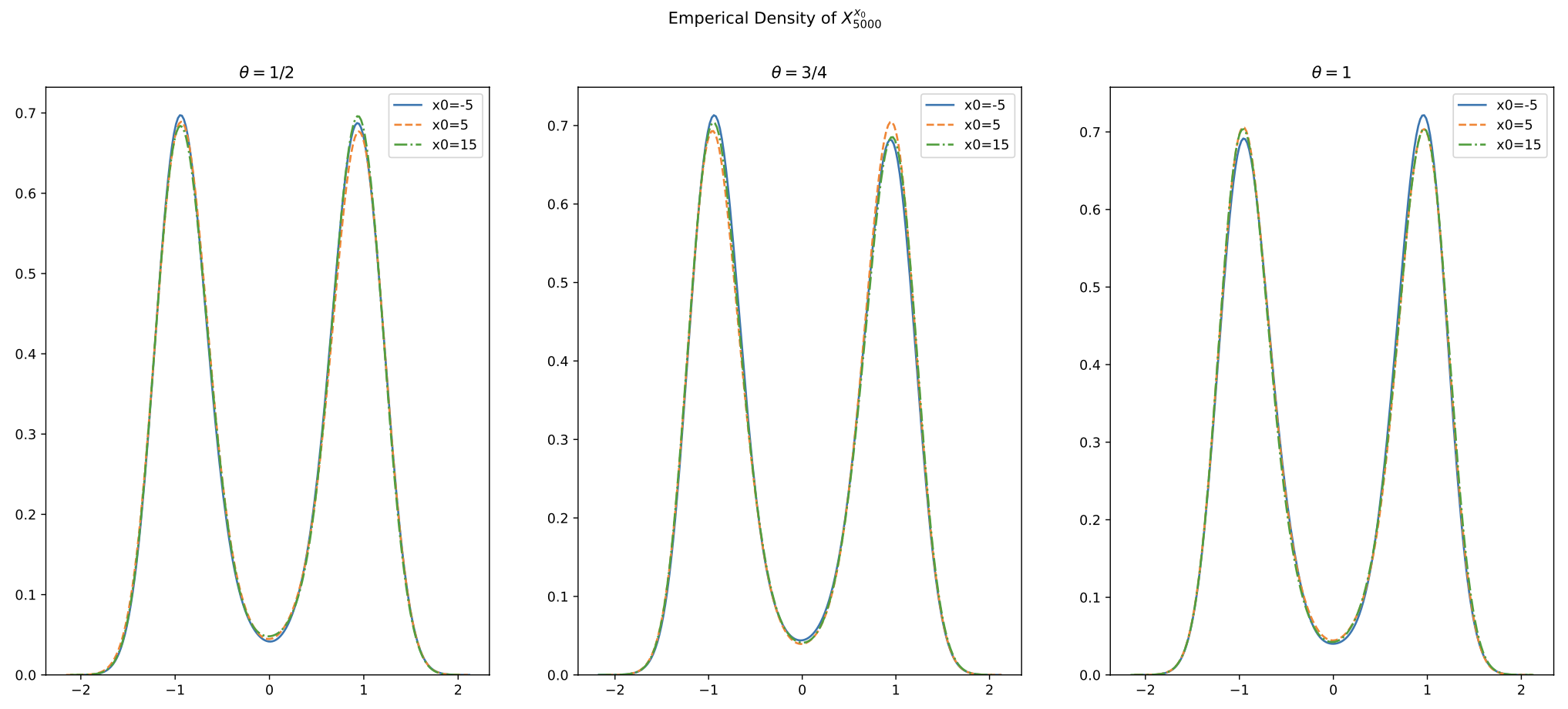
Figure 1. Empirical density of (STM) for Eq. (SDE)

The second numerical test is given to the stochastic Allen–Cahn equation (4.2) in $\mathscr{O}=(0,1)$ with $\epsilon=0.5$. By Theorem 4.5, (DIEG), including the spectral Galerkin discretization of (4.15) with $\theta=1$, is uniquely ergodic for any $\tau\in(0,1)$ (with $(\epsilon^{-2}-\lambda_{1})\tau<1$). We take $\tau=0.05$ and $N=10$ (the dimension of the spectral Galerkin approximate space), choose $\theta=1/2,3/4,1$ and initial data $X_{0}(\xi)=0,\sin\pi\xi,\sum_{k=1}^{10}\sin k\pi\xi$, $\xi\in(0,1)$, and approximate the expectation by taking averaged value over $1,000$ paths to implement the numerical experiments. In addition, we simulate the time averages $\frac{1}{2,000}\sum_{n=1}^{2,000}\mathbb{E}[\phi(X_{n})]$ (up to $n=2,000$ corresponding to $t=100$) by

$$\frac{1}{2,000,000}\sum_{n=1}^{2,000}\sum_{k=1}^{1,000}\phi(X_{n}^{k}),$$

where $X_{n}^{k}$ denotes $n$-th iteration of $k$-th sample path and the test function $\phi$ are chosen to be $\phi(\cdot)=e^{-\|\cdot\|^{2}},\sin\|\cdot\|^{2},\|\cdot\|^{2}$, respectively.

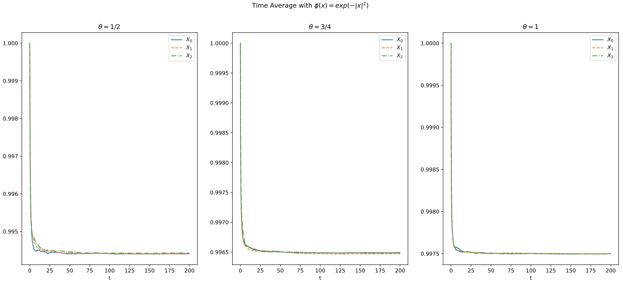
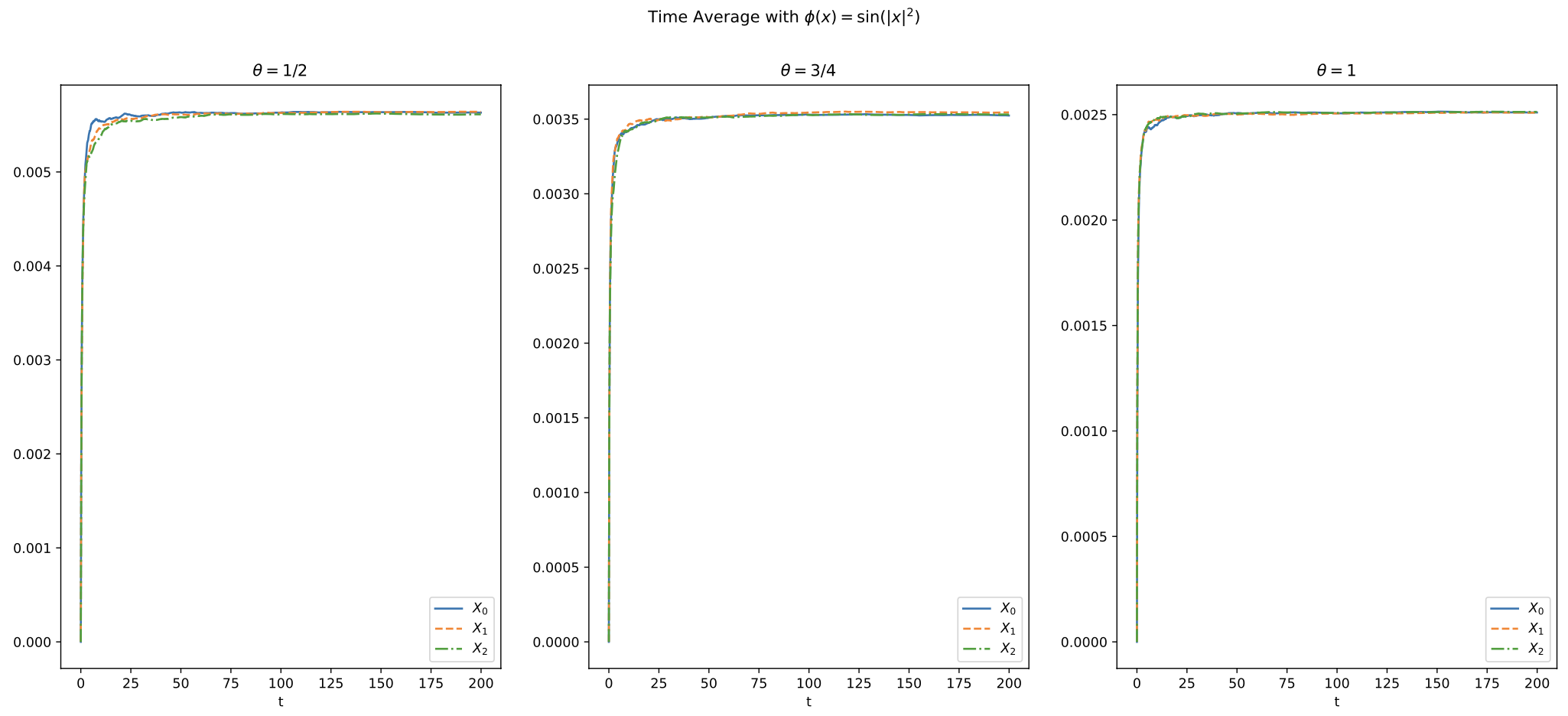
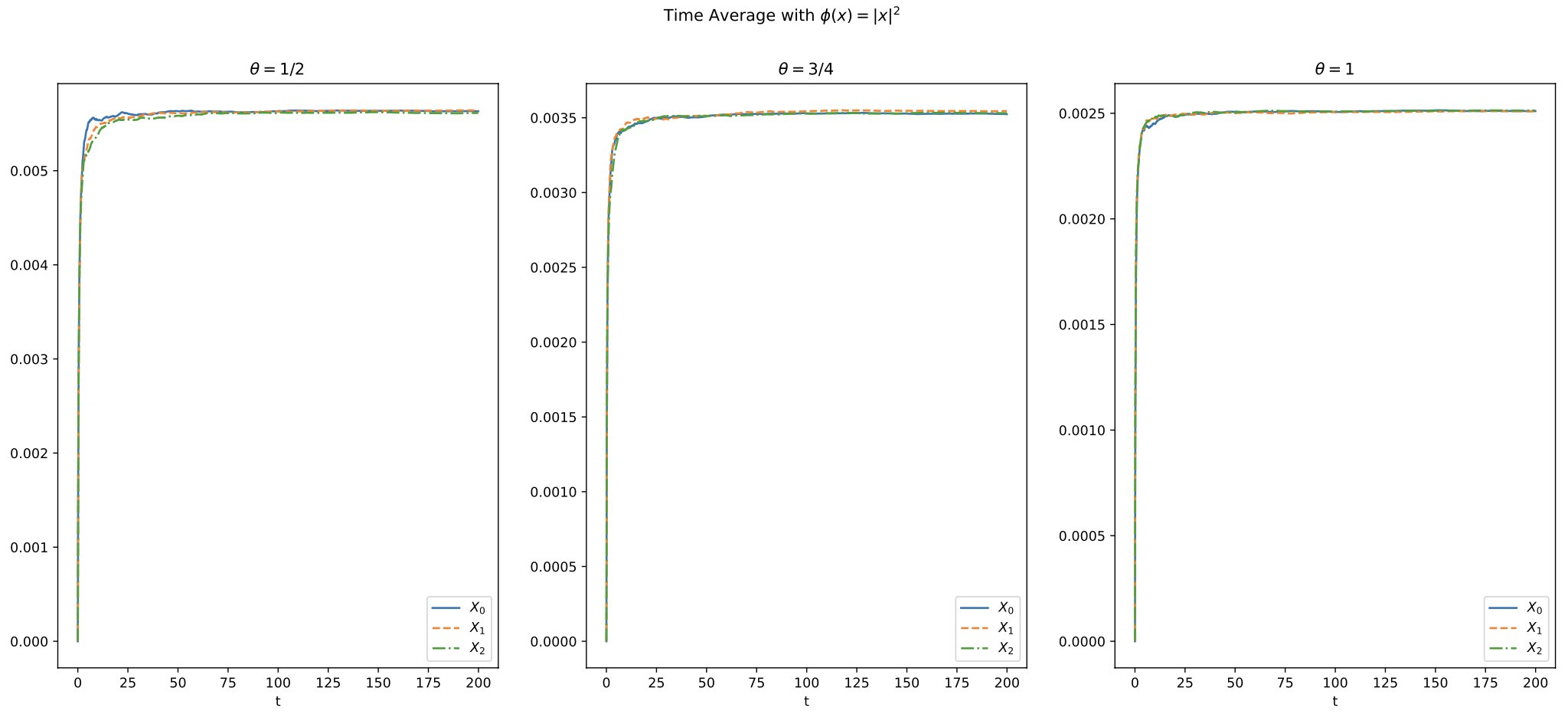
Figure 2. Time averages of (DIEG) for Eq. (4.2)

From Figure 2, the time averages of (DIEG) (with $\theta=1$) with different initial data converge to the same ergodic limit, which coincides with the theoretical result in Theorem 4.5. For other values of $\theta$ (i.e., $\theta=1/2,3/4$), Figure 2 also shows that the limiting time averages of the STM version of (DIEG) (or the Galerkin discretization of (4.15)) with the same test function but with different initial data are quite close, which indicates that the uniqueness of the ergodic limit even with different $\theta$. Indeed, these ergodic limits $\int\phi{\rm d}\pi_{\tau}^{\theta}$ are all fine approximations of $\int\phi{\rm d}\pi$, where $\pi$ is the unique invariant measure of Eq. (4.2).

6. Discussions

The theoretical loss of geometric ergodicity of (STM) with $\theta=1/2$ (in Corollary 3.2) is mainly because we can not show the stronger Lyapunov condition (3.3) at this stage. However, Figure 1 indicates that (STM) with $\theta=1/2$ is also strongly mixing. This motivates our conjecture that when $\theta=1/2$, (2.7) also holds with some $\rho\in(0,1)$ and $\kappa\geq 0$ so that it is also geometrically ergodic. On the other hand, Figure 2 indicates that (4.15) with $\theta=1/2,3/4$ and its Galerkin-based fully discretizations applied to Eq. (4.14) are also uniquely ergodic, respectively. So we conjecture that (4.15) with $\theta\in[1/2,1)$ and its Galerkin-based fully discretizations also admit similar Lyapunov structure as in (3.2) and (4.17) and that there are also uniquely ergodic, respectively. These two conjectures would be investigated in future research.

References

- [1] S. Becker, B. Gess, A. Jentzen, and P. E. Kloeden. Strong convergence rates for explicit space-time discrete numerical approximations of stochastic Allen-Cahn equations. Stoch. Partial Differ. Equ. Anal. Comput., 11(1):211–268, 2023.
- [2] S. Becker and A. Jentzen. Strong convergence rates for nonlinearity-truncated Euler-type approximations of stochastic Ginzburg-Landau equations. Stochastic Process. Appl., 129(1):28–69, 2019.
- [3] N. Bou-Rabee and E. Vanden-Eijnden. Pathwise accuracy and ergodicity of metropolized integrators for SDEs. Comm. Pure Appl. Math., 63(5):655–696, 2010.
- [4] C.-E. Bréhier. Approximation of the invariant measure with an Euler scheme for stochastic PDEs driven by space-time white noise. Potential Anal., 40(1):1–40, 2014.
- [5] C.-E. Bréhier. Approximation of the invariant distribution for a class of ergodic SPDEs using an explicit tamed exponential Euler scheme. ESAIM Math. Model. Numer. Anal., 56(1):151–175, 2022.
- [6] C.-E. Bréhier, J. Cui, and J. Hong. Strong convergence rates of semidiscrete splitting approximations for the stochastic Allen-Cahn equation. IMA J. Numer. Anal., 39(4):2096–2134, 2019.
- [7] C.-E. Bréhier and M. Kopec. Approximation of the invariant law of SPDEs: error analysis using a Poisson equation for a full-discretization scheme. IMA J. Numer. Anal., 37(3):1375–1410, 2017.
- [8] C.-E. Bréhier and G. Vilmart. High order integrator for sampling the invariant distribution of a class of parabolic stochastic PDEs with additive space-time noise. SIAM J. Sci. Comput., 38(4):A2283–A2306, 2016.
- [9] Z. Chen, S. Gan, and X. Wang. A full-discrete exponential Euler approximation of the invariant measure for parabolic stochastic partial differential equations. Appl. Numer. Math., 157:135–158, 2020.
- [10] J. Cui and J. Hong. Strong and weak convergence rates of a spatial approximation for stochastic partial differential equation with one-sided Lipschitz coefficient. SIAM J. Numer. Anal., 57(4):1815–1841, 2019.
- [11] J. Cui, J. Hong, and L. Sun. Weak convergence and invariant measure of a full discretization for parabolic SPDEs with non-globally Lipschitz coefficients. Stochastic Process. Appl., 134:55–93, 2021.
- [12] G. Da Prato and J. Zabczyk. Ergodicity for infinite-dimensional systems, volume 229 of London Mathematical Society Lecture Note Series. Cambridge University Press, Cambridge, 1996.
- [13] X. Feng, Y. Li, and Y. Zhang. Finite element methods for the stochastic Allen–Cahn equation with gradient-type multiplicative noises. SIAM J. Numer. Anal., 55(1):194–216, 2017.
- [14] I. Gyöngy and A. Millet. Rate of convergence of space time approximations for stochastic evolution equations. Potential Anal., 30(1):29–64, 2009.
- [15] M. Hairer and J. C. Mattingly. Ergodicity of the 2D Navier-Stokes equations with degenerate stochastic forcing. Ann. of Math. (2), 164(3):993–1032, 2006.
- [16] D. J. Higham, X. Mao, and A. M. Stuart. Strong convergence of Euler-type methods for nonlinear stochastic differential equation. SIAM J. Numer. Anal., 40(3):1041–1063, 2002.
- [17] J. Hong and X. Wang. Invariant measures for stochastic nonlinear Schrödinger equations, volume 2251 of Lecture Notes in Mathematics. Springer, Singapore, 2019.
- [18] M. Hutzenthaler, A. Jentzen, and P. E. Kloeden. Strong and weak divergence in finite time of Euler’s method for stochastic differential equations with non-globally Lipschitz continuous coefficients. Proc. R. Soc. Lond. Ser. A Math. Phys. Eng. Sci., 467(2130):1563–1576, 2011.
- [19] A. Jentzen and M. Röckner. A Milstein scheme for SPDEs. Found. Comput. Math., 15(2):313–362, 2015.
- [20] A. Laurent and G. Vilmart. Order conditions for sampling the invariant measure of ergodic stochastic differential equations on manifolds. Found. Comput. Math., 22(3):649–695, 2022.
- [21] X. Li, Q. Ma, H. Yang, and C. Yuan. The numerical invariant measure of stochastic differential equations with Markovian switching. SIAM J. Numer. Anal., 56(3):1435–1455, 2018.
- [22] W. Liu, X. Mao, and Y. Wu. The backward Euler-Maruyama method for invariant measures of stochastic differential equations with super-linear coefficients. Appl. Numer. Math., 184:137–150, 2023.
- [23] W. Liu and M. Röckner. Stochastic partial differential equations: an introduction. Universitext. Springer, Cham, 2015.
- [24] Z. Liu. Strong approximation of monotone SPDEs driven by multiplicative noise: exponential ergodicity and uniform estimates. arXiv:2305.06070.
- [25] Z. Liu. -convergence rate of backward Euler schemes for monotone SDEs. BIT, 62(4):1573–1590, 2022.
- [26] Z. Liu and Z. Qiao. Strong approximation of monotone stochastic partial differential equations driven by white noise. IMA J. Numer. Anal., 40(2):1074–1093, 2020.
- [27] Z. Liu and Z. Qiao. Strong approximation of monotone stochastic partial differential equations driven by multiplicative noise. Stoch. Partial Differ. Equ. Anal. Comput., 9(3):559–602, 2021.
- [28] J. C. Mattingly, A. M. Stuart, and D. J. Higham. Ergodicity for SDEs and approximations: locally Lipschitz vector fields and degenerate noise. Stochastic Process. Appl., 101(2):185–232, 2002.
- [29] S. Meyn and R. L. Tweedie. Markov chains and stochastic stability. Cambridge University Press, Cambridge, second edition, 2009.
- [30] M. Ondreját, A. Prohl, and N. J. Walkington. Numerical approximation of nonlinear SPDE’s. Stoch. Partial Differ. Equ. Anal. Comput., 11(4):1553–1634, 2023.
- [31] Q. Qiu, W. Liu, and L. Hu. Asymptotic moment boundedness of the stochastic theta method and its application for stochastic differential equations. Adv. Difference Equ., pages 2014:310, 14, 2014.
- [32] A. M. Stuart and A. R. Humphries. Dynamical systems and numerical analysis, volume 2 of Cambridge Monographs on Applied and Computational Mathematics. Cambridge University Press, Cambridge, 1996.
- [33] L. Weng and W. Liu. Invariant measures of the Milstein method for stochastic differential equations with commutative noise. Appl. Math. Comput., 358:169–176, 2019.
- [34] X. Zhang. Exponential ergodicity of non-Lipschitz stochastic differential equations. Proc. Amer. Math. Soc., 137(1):329–337, 2009.