IRS-Aided Multi-Antenna Wireless Powered Communications in Interference Channels

Abstract

This paper investigates intelligent reflecting surface (IRS)-aided multi-antenna wireless powered communications in a multi-link interference channel, where multiple IRSs are deployed to enhance the downlink/uplink communications between each pair of hybrid access point (HAP) and wireless device. Our objective is to maximize the system sum throughput by optimizing the allocation of communication resources. To attain this objective and meanwhile balance the performance-cost tradeoff, we propose three transmission schemes: the IRS-aided asynchronous (Asy) scheme, the IRS-aided time-division multiple access (TDMA) scheme, and the IRS-aided synchronous (Syn) scheme. For the resulting three non-convex design problems, we propose a general algorithmic framework capable of addressing all of them. Numerical results show that our proposed IRS-aided schemes noticeably surpass their counterparts without IRSs in both system sum throughput and total transmission energy consumption at the HAPs. Moreover, although the IRS-aided Asy scheme consistently achieves the highest sum throughput, the IRS-aided TDMA scheme is more appealing in scenarios with substantial cross-link interference and limited IRS elements, while the IRS-aided Syn scheme is preferable in low cross-link interference scenarios.

I Introduction

As a typical application of wireless power transfer (WPT), wireless powered communication network (WPCN) is viewed as a promising network paradigm to address the energy shortage problem of wireless devices (WDs). In [1], the authors studied a single-input single-output (SISO) WPCN and proposed the well-known “harvest-then-transmit” protocol. This work was then extended to more general single-cell multi-antenna WPCNs in [2] and [3], and a multi-cell SISO WPCN in [4], respectively. Despite theoretical progress, practical WPCNs face severe limitations due to the low efficiencies of WPT over long transmission distances. Recently, intelligent reflecting surface (IRS) [5] has emerged as an effective remedy to tackle this performance bottleneck. The results in [6] indicated that introducing an IRS into a SISO WPCN has the dual benefits of enhancing the system throughput and lowering the energy consumption at the hybrid access point (HAP). Additionally, the authors of [7] and [8] confirmed that the IRS can improve the performance of multi-antenna WPCNs.

However, all the above-mentioned works on IRS-assisted WPCNs are limited to single-cell scenarios. To the best of the authors’ knowledge, the potential performance gain of integrating IRSs into multi-cell WPCNs in interference channels (IFCs) has not been explored yet. Recall that the authors of [4] studied a traditional multi-cell SISO WPCN. Their simulation results demonstrated that an asynchronous protocol involving asynchronous downlink (DL)-uplink (UL) time allocation for different cells can lead to a larger system sum throughput compared to its synchronous counterpart. Intuitively, introducing IRSs can enlarge the performance gap between these two protocols, since the presence of more transmission phases in the asynchronous protocol allows more opportunities for IRS reconfigurations (and therefore radio propagation environment reconfigurations). New resource allocation designs are necessary for the case with IRSs, as those proposed in [4] are not applicable. Moreover, the work in [4] has certain limitations. First, it was confined to a SISO setting without harnessing the multi-antenna technology to improve the system performance. Second, it did not disclose whether the performance gain achieved by the asynchronous protocol comes with higher energy costs, a factor that influences the selection of transmission protocols in practice.

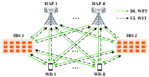
Figure 1: Illustration of IRS-aided multi-antenna wireless powered communications in an interference channel.

Motivated by the above considerations, this paper studies an IRS-aided multi-antenna wireless powered IFC, comprising multiple IRSs and HAP-WD pairs. To maximize the system sum throughput while considering the balance between performance and cost, we propose three transmission schemes: the IRS-aided asynchronous (Asy) scheme, the IRS-aided time-division multiple access (TDMA) scheme, and the IRS-aided synchronous (Syn) scheme, ranked from high to low in terms of implementation complexity. Theoretically, the IRS-aided Asy scheme always attains the highest sum throughput, as it is a super-scheme of the other two. In addition, neither the IRS-aided TDMA scheme nor the IRS-aided Syn scheme can consistently outperform the other in terms of system sum throughput. This is mainly because the IRS-aided TDMA scheme enjoys the advantage of being free from cross-channel interference in uplink wireless information transfer (WIT) but grapples with the inefficient utilization of time resources. This scheme’s advantage tends to diminish or even disappear in scenarios with low cross-link interference and/or sufficient IRS elements in the IRS-aided Syn scheme, while its drawback remains challenging to overcome even with an increased number of IRS elements. Nevertheless, theoretically ranking the energy consumption of these three schemes is difficult. We propose a general algorithmic framework to solve the three corresponding resource allocation problems and numerically evaluate the performance of the three schemes. Simulation results verify the above discussions regarding performance comparisons and show that the IRS-aided TDMA scheme consumes the most energy while the IRS-aided Syn scheme consumes the least. After a comprehensive evaluation of performance, implementation complexity, and energy cost, we find that the IRS-aided TDMA scheme is most appealing in scenarios with overwhelming cross-link interference and limited IRS elements, the IRS-aided Syn scheme is the best choice when cross-link interference is low, and the IRS-aided Asy scheme is preferable in all other scenarios.

II System Model and Problem Formulation

II-A System Model

As shown in Fig. 1, we consider a narrow-band IRS-aided wireless powered IFC, where $K$ pairs of $M$-antenna HAPs and single-antenna WDs operate over the same frequency band with the aid of $L$ passive IRSs. The $\ell$-th IRS is equipped with $N_{\ell}$ elements. The sets of HAP-WD pairs, IRSs, and all the IRS elements are denoted as $\mathcal{K}$, $\mathcal{L}$, and $\mathcal{N}$, respectively, with $\left|\mathcal{K}\right|=K$, $\left|\mathcal{L}\right|=L$, and $\left|\mathcal{N}\right|=N=\sum_{\ell=1}^{L}N_{\ell}$. The UL channels from WD $k$ to IRS $\ell$, from IRS $\ell$ to HAP $i$, and from WD $k$ to HAP $i$ are denoted by $\mathbf{e}_{k,\ell}\in\mathbb{C}^{N_{\ell}\times 1}$, $\mathbf{H}_{\ell,i}\in\mathbb{C}^{M\times N_{\ell}}$, and $\mathbf{g}_{k,i}\in\mathbb{C}^{M\times 1}$, respectively, which remain constant throughout the total transmission time $T$. Moreover, the UL-DL channel reciprocity is assumed.

II-A1 IRS-Aided Asy Scheme

Following the typical “harvest-then-transmit” protocol [1], WD $k$ performs EH first and then WIT, with durations of $\tau_{k}$ and $T-\tau_{k}$, respectively. Without loss of generality, we assume that $\{\tau_{k}\}$ are sorted in an ascending order, i.e., $\tau_{1}\leq\tau_{2}\leq\dots\leq\tau_{K}$. According to the WDs’ operations, the entire transmission process can be divided into $K+1$ phases, as illustrated in Fig. 2. We define $\delta_{j}\triangleq\tau_{j}-\tau_{j-1}$ as the time duration of phase $j$ ($j\in\mathcal{J}\triangleq\{1,\cdots,K+1\}$), where $\tau_{0}\triangleq 0$ and $\tau_{K+1}\triangleq T$. Denoted by $\mathbf{\Theta}_{\ell,j}={\rm diag}\left(\beta_{\ell,1,j}e^{\jmath\theta_{\ell,1,j}},\cdots,\beta_{\ell,N_{\ell},j}e^{\jmath\theta_{\ell,N_{\ell},j}}\right)$ the reflection-coefficient matrix at IRS $\ell$ in phase $j$, where $\beta_{\ell,n,j}$ and $\theta_{\ell,n,j}$ can be independently adjusted over $[0,1]$ and $[0,2\pi)$, respectively [9]. Besides, let $\mbox{\boldmath{$x$}}_{i,j}\in\mathbb{C}^{M\times 1}$ denote the energy signal vector transmitted by HAP $i$ in phase $j$ ($j=1,\cdots,i$), with a covariance matrix $\mathbf{S}_{i,j}=\mathbb{E}\left(\mbox{\boldmath{$x$}}_{i,j}\mbox{\boldmath{$x$}}_{i,j}^{H}\right)\succeq\mathbf{0}$.

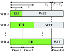
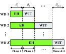
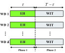
Figure 2: Illustration of three different transmission schemes: (a) IRS-aided Asy scheme; (b) IRS-aided TDMA scheme; (c) IRS-aided Syn scheme.

In phase $1$, all the HAPs are engaged in WPT. The received signal at WD $k$, $k\in\mathcal{K}$, in this phase is given by $y_{k,1}^{\rm E}=\sum_{i=1}^{K}\left(\sum_{\ell=1}^{L}\mathbf{H}_{\ell,i}\mathbf{\Theta}_{\ell,1}\mathbf{e}_{k,\ell}+\mathbf{g}_{k,i}\right)^{T}\mbox{\boldmath{$x$}}_{i,1}+n_{k}=\sum_{i=1}^{K}\left(\mathbf{H}_{i}\mathbf{\Theta}_{1}\mathbf{e}_{k}+\mathbf{g}_{k,i}\right)^{T}\mbox{\boldmath{$x$}}_{i,1}+n_{k}=\sum_{i=1}^{K}\mathbf{v}_{1}^{T}\mathbf{\Psi}_{k,i}^{T}\mbox{\boldmath{$x$}}_{i,1}+n_{k}$, where $n_{k}$ stands for the additive white Gaussian noise (AWGN) at WD $k$, $\mathbf{H}_{i}=\left[\mathbf{H}_{1,i},\cdots,\mathbf{H}_{L,i}\right]$, $\mathbf{\Theta}_{1}={\rm blkdiag}\left(\mathbf{\Theta}_{1,1},\cdots,\mathbf{\Theta}_{L,1}\right)$, $\mathbf{e}_{k}=\left[\mathbf{e}_{k,1};\cdots;\mathbf{e}_{k,L}\right]$, $\mathbf{v}_{1}=\left[{\rm Diag}\left(\mathbf{\Theta}_{1}\right);1\right]$, and $\mathbf{\Psi}_{k,i}=\left[\mathbf{H}_{i}{\rm diag}\left(\mathbf{e}_{k}\right),\mathbf{g}_{k,i}\right]$. Note that the signals experiencing multiple reflections are disregarded due to the multiplicative path loss. By ignoring the negligible noise power, the energy harvested by MD $k$ in the 1st phase can be written as $E_{k,1}=\eta\delta_{1}\sum_{i=1}^{K}{\rm tr}\left(\mathbf{\Psi}_{k,i}^{*}\mathbf{v}_{1}^{*}\mathbf{v}_{1}^{T}\mathbf{\Psi}_{k,i}^{T}\mathbf{S}_{i,1}\right)$, with $\eta$ denoting the energy conversion efficiency of each WD.

In the subsequent phase $j$ ($j=2,\cdots,K$), HAPs $\{i^{\prime}|i^{\prime}=j,\cdots,K\}$ continue to broadcast energy, whereas HAPs $\{i|i=1,\cdots,j-1\}$ receive UL information signals from WDs $\{k|k=1,\cdots,j-1\}$. The received signal at HAP $i$ in phase $j$ can be expressed as $\mathbf{y}_{i,j}^{\rm I}=\sum_{k=1}^{j-1}\left(\sum_{\ell=1}^{L}\mathbf{H}_{\ell,i}\mathbf{\Theta}_{\ell,j}\mathbf{e}_{k,\ell}+\mathbf{g}_{k,i}\right)\sqrt{p_{k,j}}s_{k}+\boldsymbol{\iota}^{\rm E}_{i,j}+\hat{\mathbf{n}}_{i}=\sum_{k=1}^{j-1}\mathbf{\Psi}_{k,i}\mathbf{v}_{j}\sqrt{p_{k,j}}s_{k}+\boldsymbol{\iota}^{\rm E}_{i,j}+\hat{\mathbf{n}}_{i}$, where $p_{k,j}$ denotes the UL transmit power of WD $k$ in phase $j$, $s_{k}\in\mathbb{C}$ is the transmitted data symbol of WD $k$ satisfying $s_{k}\sim\mathcal{CN}\left(0,1\right)$, $\boldsymbol{\iota}^{\rm E}_{i,j}$ stands for the DL-to-UL interference caused by the energy signals from HAPs $\{i^{\prime}|i^{\prime}=j,\cdots,K\}$, $\mathbf{v}_{j}=\left[{\rm Diag}\left(\mathbf{\Theta}_{j}\right);1\right]$ with $\mathbf{\Theta}_{j}={\rm blkdiag}\left(\mathbf{\Theta}_{1,j},\cdots,\mathbf{\Theta}_{L,j}\right)$, and $\hat{\mathbf{n}}_{i}\in\mathbb{C}^{M\times 1}$ represents the zero-mean AWGN at HAP $i$ with co-variance matrix $\sigma_{i}^{2}\mathbf{I}_{M}$. By assuming that the HAPs employ linear receivers to decode $\{s_{k}\}$, we denote $\mathbf{w}_{i,j}\in\mathbb{C}^{M\times 1}$ as the unit-norm receive beamforming vector at HAP $i$ for decoding $s_{i}$ in phase $j$. Additionally, we assume that the energy signals are known deterministic signals, enabling HAP $i$ to cancel the energy signal interference. Consequently, the achievable rate at HAP $i$ in bits/Hz during phase $j$ ($j=i+1,\cdots,K$) is obtained as $R_{i,j}=\delta_{j}\log_{2}\left(1+\gamma_{i,j}\right)$ with

$$\gamma_{i,j}=\frac{p_{i,j}\left|\mathbf{w}_{i,j}^{H}\mathbf{\Psi}_{i,i}\mathbf{v}_{j}\right|^{2}}{\sum_{k=1,k\neq i}^{j-1}p_{k,j}\left|\mathbf{w}_{i,j}^{H}\mathbf{\Psi}_{k,i}\mathbf{v}_{j}\right|^{2}+\sigma_{i}^{2}\left\|\mathbf{w}_{i,j}\right\|^{2}}.$$ (1)

Meanwhile, WDs $\{k|k=j,\cdots,K\}$ harvest energy in phase $j$ ($j=2,\cdots,K$). For the EH at WD $k$, we ignore the UL WIT signal power from other WDs and the noise power, as both are negligible compared to the HAP transmit power. Then, the energy collected by WD $k$ in phase $j$ can be expressed as $E_{k,j}=\eta\delta_{j}\sum_{i=j}^{K}{\rm tr}\left(\mathbf{\Psi}_{k,i}^{*}\mathbf{v}_{j}^{*}\mathbf{v}_{j}^{T}\mathbf{\Psi}_{k,i}^{T}\mathbf{S}_{i,j}\right)$.

In the final phase, all the WDs execute the WIT operation. The achievable rate at HAP $i$ is given by $R_{i,K+1}=\delta_{K+1}\log_{2}\left(1+\gamma_{i,K+1}\right)$, where the expression of $\gamma_{i,K+1}$ can be obtained by replacing the index “$j$” in (1) by “$K+1$”.

II-A2 IRS-Aided TDMA Scheme

For the scheme shown in Fig. 2, the WDs perform UL WIT in a TDMA manner. This scheme is a special case of the IRS-aided Asy scheme with $p_{k,j}=0$ and $\mathbf{w}_{i,j}=\mathbf{0}$, $\forall k,i\in\mathcal{K},j\in\mathcal{J}\backslash\{k+1\}$.

II-A3 IRS-Aided Syn Scheme

When $\tau_{k}=\tau$, $\forall k\in\mathcal{K}$, the IRS-aided Asy scheme boils down to the IRS-aided Syn scheme, as illustrated in Fig. 2.

II-B Problem Formulation

For the IRS-aided Asy scheme, the sum throughput maximization problem can be formulated as

$$\text{(P1)}: \underset{\mathcal{Z}}{\max} \sum_{i=1}^{K}\sum_{j=i+1}^{K+1}R_{i,j}$$ (2a)

s.t. $$\sum_{j=k+1}^{K+1}\delta_{j}p_{k,j}\leq\sum_{j=1}^{k}E_{k,j},\forall k\in\mathcal{K},$$ (2f)

$$\sum_{j=1}^{K+1}\delta_{j}\leq T,$$

$${\rm tr}\left(\mathbf{S}_{i,j}\right)\leq P_{i},\forall i\in\mathcal{K},j=1,\cdots,i,$$

$$\left\|\mathbf{w}_{i,j}\right\|^{2}=1,\forall i\in\mathcal{K},j=i+1,\cdots,K+1,$$

$$\left|\left[\mathbf{v}_{j}\right]_{n}\right|\leq 1,\ \left[\mathbf{v}_{j}\right]_{N+1}=1,\ \forall n\in\mathcal{N},j\in\mathcal{J},$$

where $\mathcal{Z}\triangleq\left\{\{\delta_{j}\geq 0\},\{\mathbf{S}_{i,j}\succeq\mathbf{0}\},\{p_{k,j}\geq 0\},\{\mathbf{w}_{i,j}\},\{\mathbf{v}_{j}\}\right\}$ is composed of all the optimization variables, including the time allocation, the DL energy variance matrices, the UL power allocation, the UL receive beamforming vectors, and the IRS reflect beamforming vectors. Furthermore, (2f) and (2f) denote the energy causality and total time constraints, respectively, $P_{i}$ in (2f) represents the maximum instantaneous transmit power of HAP $k$, (2f) means that $\{\mathbf{w}_{i,j}\}$ have unit norms, and (2f) imposes modulus constraints on the IRS bemaforming vectors. Similarly, we can formulate the sum throughput maximization problems for the IRS-aided TDMA and Syn schemes, respectively, denoted by (P2) and (P3). The formulations of these two problems are omitted due to the space limitation. We note that the coupling of the optimization variables presents a challenge in solving (P1)-(P3) optimally. To this end, we propose a general algorithmic framework based on the alternating optimization technique, applicable to solving all of these problems suboptimally, as detailed in the following section.

III Proposed General Algorithmic Framework for (P1)-(P3)

III-A How To Solve (P1)?

Based on the principle of alternating optimization, we partition the optimization variables into three blocks, i.e., $\{\mathbf{w}_{i,j}\}$, $\left\{\{\delta_{j}\},\{\mathbf{S}_{i,j}\},\{p_{k,j}\}\right\}$, and $\{\mathbf{v}_{j}\}$. These blocks are updated alternately until convergence is achieved, as elaborated below.

III-A1 Optimizing $\{\mathbf{w}_{i,j}\}$

When given other variables, the optimization of $\{\mathbf{w}_{i,j}\}$ can be performed independently and in parallel for each $\mathbf{w}_{i,j}$. Specifically, we can calculate $\mathbf{w}_{i,j}$ using

$$\mathbf{w}_{i,j}^{\star} =\underset{\left\|\mathbf{w}_{i,j}\right\|^{2}=1}{\rm arg\max}\hskip 4.2679pt\frac{p_{i,j}\left|\mathbf{w}_{i,j}^{H}\mathbf{a}_{i,i,j}\right|^{2}}{\sum_{k=1,k\neq i}^{j-1}p_{k,j}\left|\mathbf{w}_{i,j}^{H}\mathbf{a}_{k,i,j}\right|^{2}+\sigma_{i}^{2}\left\|\mathbf{w}_{i,j}\right\|^{2}}$$

$$=\frac{\left(\sum_{k=1}^{j-1}p_{k,j}\mathbf{a}_{k,i,j}\mathbf{a}_{k,i,j}^{H}+\sigma_{i}^{2}\mathbf{I}_{M}\right)^{-1}\mathbf{a}_{i,i,j}}{\left\|\left(\sum_{k=1}^{j-1}p_{k,j}\mathbf{a}_{k,i,j}\mathbf{a}_{k,i,j}^{H}+\sigma_{i}^{2}\mathbf{I}_{M}\right)^{-1}\mathbf{a}_{i,i,j}\right\|},$$ (3)

where $\mathbf{a}_{k,i,j}\triangleq\mathbf{\Psi}_{k,i}\mathbf{v}_{j}$, $\forall k,i\in\mathcal{K},j=i+1,\cdots,K+1$.

III-A2 Optimizing $\left\{\{\delta_{j}\},\{\mathbf{S}_{i,j}\},\{p_{k,j}\}\right\}$

For given $\{\mathbf{w}_{i,j}\}$ and $\{\mathbf{v}_{j}\}$, the remaining variables can be optimized by solving

$$\underset{\begin{subarray}{c}\{\delta_{j}\geq 0\},\{\mathbf{S}_{i,j}\succeq\mathbf{0}\},\\ \{p_{k,j}\geq 0\}\end{subarray}}{\max}\hskip 5.69054pt\sum_{i=1}^{K}\sum_{j=i+1}^{K+1}\delta_{j}r_{i,j}\hskip 11.38109pt\text{s.t.}\hskip 5.69054pt\eqref{P1_cons:b}-\eqref{P1_cons:d},$$ (4)

where $r_{i,j}\triangleq\log_{2}\left(1+\frac{p_{i,j}b_{i,i,j}}{\sum_{k=1,k\neq i}^{j-1}p_{k,j}b_{k,i,j}+\sigma_{i}^{2}}\right)$ with $b_{k,i,j}\triangleq\left|\mathbf{w}_{i,j}^{H}\mathbf{\Psi}_{k,i}\mathbf{v}_{j}\right|^{2}$, $\forall k,i\in\mathcal{K},j=i+1,\cdots,K+1$. Problem (4) exhibits non-convexity stemming from the non-concave nature of the objective function and the non-convex constraint (2f). To facilitate the solution design, we reformulate the objective function as $\sum_{i=1}^{K}\sum_{j=i+1}^{K+1}\delta_{j}\left(f_{i,j}-g_{i,j}\right)$, where both $f_{i,j}$ and $g_{i,j}$ are concave functions defined by $f_{i,j}\triangleq\log_{2}\left(\sum_{k=1}^{j-1}p_{k,j}b_{k,i,j}+\sigma_{i}^{2}\right)$ and $g_{i,j}\triangleq\log_{2}\left(\sum_{k=1,k\neq i}^{j-1}p_{k,j}b_{k,i,j}+\sigma_{i}^{2}\right)$, respectively. The fact that the first-order Taylor expansion of any concave function at any point is its global upper bound motivates the utilization of the successive convex approximation (SCA) to tackle this issue. To be specific, with given local points $\{p_{k,j}^{t}\}$ in the $t$-th iteration, we have $g_{i,j}\left(\{p_{k,j}\}\right)\leq g_{i,j}\big{(}\{p_{k,j}^{t}\}\big{)}+\frac{\sum_{k=1,k\neq i}^{j-1}b_{k,i,j}\left(p_{k,j}-p_{k,j}^{t}\right)}{\left(\sum_{k=1,k\neq i}^{j-1}p_{k,j}^{t}b_{k,i,j}+\sigma_{i}^{2}\right)\ln 2}\triangleq g_{i,j}^{\rm ub,\it t}\left(\{p_{k,j}\}\right)$. Then, a lower bound of the optimal value of problem (4) can be acquired by solving

$$\underset{\begin{subarray}{c}\{\delta_{j}\geq 0\},\{\mathbf{S}_{i,j}\succeq\mathbf{0}\},\\ \{p_{k,j}\geq 0\}\end{subarray}}{\max} \sum_{i=1}^{K}\sum_{j=i+1}^{K+1}\delta_{j}\left(f_{i,j}-g_{i,j}^{\rm ub,\it t}\left(\{p_{k,j}\}\right)\right)$$ (5a)

s.t. $$\eqref{P1_cons:b}-\eqref{P1_cons:d},$$ (5b)

which is still non-convex. Nevertheless, by applying the change of variables $\tilde{p}_{k,j}=\delta_{j}p_{k,j}$, $\forall k\in\mathcal{K},j=k+1,\cdots,K+1$, and $\tilde{\mathbf{S}}_{i,j}=\delta_{j}\mathbf{S}_{i,j}$, $\forall i\in\mathcal{K},j=1,\cdots,i$, problem (5) can be equivalently written as

$$\underset{\begin{subarray}{c}\{\delta_{j}\geq 0\},\{\tilde{\mathbf{S}}_{i,j}\succeq\mathbf{0}\},\\ \{\tilde{p}_{k,j}\geq 0\}\end{subarray}}{\max}\hskip 5.69054pt\sum_{i=1}^{K}\sum_{j=i+1}^{K+1}R_{i,j}^{\rm lb,\it t}$$ (6a)

s.t. $$\hskip 2.84526pt\sum_{j=k+1}^{K+1}\tilde{p}_{k,j}\leq\sum_{j=1}^{k}\eta\delta_{j}\sum_{i=j}^{K}{\rm tr}\left(\mathbf{A}_{k,i,j}\tilde{\mathbf{S}}_{i,j}\right),\forall k\in\mathcal{K},$$ (6b)

$$\hskip 2.84526pt{\rm tr}\left(\tilde{\mathbf{S}}_{i,j}\right)\leq\delta_{j}P_{i},\forall i\in\mathcal{K},j=1,\cdots,i,\hskip 5.69054pt\eqref{P1_cons:c},$$ (6c)

where $R_{i,j}^{\rm lb,\it t}\!\triangleq\!\delta_{j}\log_{2}\left(\frac{\sum_{k=1}^{j-1}\tilde{p}_{k,j}b_{k,i,j}}{\delta_{j}}+\sigma_{i}^{2}\right)-\delta_{j}g_{i,j}\big{(}\{p_{k,j}^{t}\}\big{)}\!-\!\frac{\sum_{k=1,k\neq i}^{j-1}b_{k,i,j}\left(\tilde{p}_{k,j}-\delta_{j}p_{k,j}^{t}\right)}{\left(\sum_{k=1,k\neq i}^{j-1}p_{k,j}^{t}b_{k,i,j}+\sigma_{i}^{2}\right)\ln 2}$ and $\mathbf{A}_{k,i,j}\triangleq\mathbf{\Psi}_{k,i}^{*}\mathbf{v}_{j}^{*}\mathbf{v}_{j}^{T}\mathbf{\Psi}_{k,i}^{T}$. As a convex semi-definite program (SDP), problem (6) can be directly solved using standard solvers such as CVX.

III-A3 Optimizing $\{\mathbf{v}_{j}\}$

Given other variables, we now focus on optimizing $\{\mathbf{v}_{j}\}$. We particularly note that, unlike $\{\mathbf{v}_{j}\}_{j\in\mathcal{J}\backslash\{1\}}$, which are involved in both the objective function and constraints, $\mathbf{v}_{1}$ only exists in the constraints. Therefore, $\mathbf{v}_{1}$ and $\hat{\mathbf{v}}\triangleq\{\mathbf{v}_{j}\}_{j\in\mathcal{J}\backslash\{1\}}$ are optimized sequentially using distinct approaches as follows.

Optimizing $\mathbf{v}_{1}$

The subproblem with respect to (w.r.t.) $\mathbf{v}_{1}$ is a feasibility-check problem. To obtain a more efficient solution, we introduce the “EH residual” variables $\{\Delta_{k}\}$, and then arrive at the following problem

$$\underset{\mathbf{v}_{1},\{\Delta_{k}\geq 0\}}{\max} \sum_{k=1}^{K}\Delta_{k}$$ (7c)

s.t. $$\sum_{j=k+1}^{K+1}\delta_{j}p_{k,j}+\Delta_{k}\leq\eta\delta_{1}\sum_{i=1}^{K}\mathbf{v}_{1}^{T}\mathbf{C}_{k,i,1}\mathbf{v}_{1}^{*}$$

$$+\sum_{j=2}^{k}\eta\delta_{j}\sum_{i=j}^{K}\mathbf{v}_{j}^{T}\mathbf{C}_{k,i,j}\mathbf{v}_{j}^{*},\forall k\in\mathcal{K},$$

$$\left|\left[\mathbf{v}_{1}\right]_{n}\right|\leq 1,\ \left[\mathbf{v}_{1}\right]_{N+1}=1,\ \forall n\in\mathcal{N},$$

where $\mathbf{C}_{k,i,j}\triangleq\mathbf{\Psi}_{k,i}^{T}\mathbf{S}_{i,j}\mathbf{\Psi}_{k,i}^{*}$, $\forall i,k\in\mathcal{K},j=1,\cdots,k$. The convex nature of $\mathbf{v}_{1}^{T}\mathbf{C}_{k,i,1}\mathbf{v}_{1}^{*}$ in (7c) leads to the non-convexity of problem (7) but permits the use of SCA. With a given local point $\mathbf{v}_{1}^{t}$ in the $t$-th iteration, $\mathbf{v}_{1}^{T}\mathbf{C}_{k,i,1}\mathbf{v}_{1}^{*}$ is lower bounded by its first-order Taylor expansion, denoted by $\mathcal{E}_{\mathbf{C}_{k,i,1}}^{\rm lb,\it t}(\mathbf{v}_{1})\triangleq 2{\rm Re}\left\{\left(\mathbf{v}_{1}^{t}\right)^{T}\mathbf{C}_{k,i,1}\mathbf{v}_{1}^{*}\right\}-\left(\mathbf{v}_{1}^{t}\right)^{T}\mathbf{C}_{k,i,1}\left(\mathbf{v}_{1}^{t}\right)^{*}$. By replacing $\mathbf{v}_{1}^{T}\mathbf{C}_{k,i,1}\mathbf{v}_{1}^{*}$ with $\mathcal{E}_{\mathbf{C}_{k,i,1}}^{\rm lb,\it t}(\mathbf{v}_{1})$, problem (7) can be approximated as

$$\underset{\mathbf{v}_{1},\{\Delta_{k}\geq 0\}}{\max} \sum_{k=1}^{K}\Delta_{k}$$ (8b)

s.t. $$\sum_{j=k+1}^{K+1}\delta_{j}p_{k,j}+\Delta_{k}\leq\eta\delta_{1}\sum_{i=1}^{K}\mathcal{E}_{\mathbf{C}_{k,i,1}}^{\rm lb,\it t}(\mathbf{v}_{1})$$

$$+\sum_{j=2}^{k}\eta\delta_{j}\sum_{i=j}^{K}\mathbf{v}_{j}^{T}\mathbf{C}_{k,i,j}\mathbf{v}_{j}^{*},\forall k\in\mathcal{K},\hskip 5.69054pt\eqref{P1-sub31_cons:c},$$

which is a convex quadratically constrained quadratic program (QCQP) and can be efficiently solved by CVX.

Optimizing $\hat{\mathbf{v}}$

To proceed, we optimize $\hat{\mathbf{v}}$. By introducing slack variables $\{z_{i,j}\}$, the subproblem w.r.t. $\hat{\mathbf{v}}$ can be equivalently converted to

$$\underset{\hat{\mathbf{v}},\{z_{i,j}\}}{\max} \sum_{i=1}^{K}\sum_{j=i+1}^{K+1}\delta_{j}\log_{2}\left(1+z_{i,j}\right)$$ (9d)

s.t. $$\frac{\mathbf{v}_{j}^{H}\mathbf{B}_{i,i,j}\mathbf{v}_{j}}{z_{i,j}}\geq\sum_{k=1,k\neq i}^{j-1}\mathbf{v}_{j}^{H}\mathbf{B}_{k,i,j}\mathbf{v}_{j}+\sigma_{i}^{2},$$

$$\forall i\in\mathcal{K},j=i+1,\cdots,K+1,$$

$$\sum_{j=k+1}^{K+1}\delta_{j}p_{k,j}\leq\eta\delta_{1}\sum_{k=1}^{K}\mathbf{v}_{1}^{T}\mathbf{C}_{k,i,1}\mathbf{v}_{1}^{*}$$

$$+\sum_{j=2}^{k}\eta\delta_{j}\sum_{i=j}^{K}\mathbf{v}_{j}^{T}\mathbf{C}_{k,i,j}\mathbf{v}_{j}^{*},\forall k\in\mathcal{K},$$

$$\left|\left[\mathbf{v}_{j}\right]_{n}\right|\leq 1,\ \left[\mathbf{v}_{j}\right]_{N+1}=1,\ \forall n\in\mathcal{N},j\in\mathcal{J}\backslash\{1\},$$

where $\mathbf{B}_{k,i,j}\triangleq p_{k,j}\mathbf{\Psi}_{k,i}^{H}\mathbf{w}_{i,j}\mathbf{w}_{i,j}^{H}\mathbf{\Psi}_{k,i}$, $\forall k,i\in\mathcal{K},j=i+1,\cdots,K+1$. The non-convexity of problem (9) arises from the convex terms $\frac{\mathbf{v}_{j}^{H}\mathbf{B}_{i,i,j}\mathbf{v}_{j}}{z_{i,j}}$ and $\mathbf{v}_{j}^{T}\mathbf{C}_{k,i,j}\mathbf{v}_{j}^{*}$, which prompts us to substitute these convex terms by their first-order Taylor expansion-based affine under-estimators. In this way, the problem to be solved becomes the following convex QCQP:

$$\underset{\hat{\mathbf{v}_{j}},\{z_{i,j}\}}{\max} \sum_{i=1}^{K}\sum_{j=i+1}^{K+1}\delta_{j}\log_{2}\left(1+z_{i,j}\right)$$ (10c)

s.t. $$\mathcal{F}_{\mathbf{B}_{i,i,j}}^{\rm lb,\it t}(\mathbf{v}_{j},z_{i,j})\geq\sum_{k=1,k\neq i}^{j-1}\mathbf{v}_{j}^{H}\mathbf{B}_{k,i,j}\mathbf{v}_{j}+\sigma_{i}^{2},$$

$$\forall i\in\mathcal{K},j=i+1,\cdots,K+1,$$

$$\sum_{j=k+1}^{K+1}\delta_{j}p_{k,j}\leq\eta\delta_{1}\sum_{k=1}^{K}\mathbf{v}_{1}^{T}\mathbf{C}_{k,i,1}\mathbf{v}_{1}^{*}$$

$$+\sum_{j=2}^{k}\eta\delta_{j}\sum_{i=j}^{K}\mathcal{E}_{\mathbf{C}_{k,i,j}}^{\rm lb,\it t}(\mathbf{v}_{j}),\forall k\in\mathcal{K},\hskip 5.69054pt\eqref{P1-sub32_cons:d},$$

where $\mathcal{F}_{\mathbf{B}_{i,i,j}}^{\rm lb,\it r}(\mathbf{v}_{j},z_{i,j})\!\triangleq\!\frac{2{\rm Re}\left\{(\mathbf{v}_{j}^{t})^{H}\mathbf{B}_{i,i,j}\mathbf{v}_{j}\right\}}{z_{i,j}^{t}}\!-\!\frac{(\mathbf{v}_{j}^{t})^{H}\mathbf{B}_{i,i,j}\mathbf{v}_{j}^{t}}{\left(z_{i,j}^{t}\right)^{2}}z_{i,j}$ and $\mathcal{E}_{\mathbf{C}_{k,i,j}}^{\rm lb,\it t}(\mathbf{v}_{j})\triangleq 2{\rm Re}\left\{(\mathbf{v}_{j}^{t})^{T}\mathbf{C}_{k,i,j}\mathbf{v}_{j}^{*}\right\}-(\mathbf{v}_{j}^{t})^{T}\mathbf{C}_{k,i,j}(\mathbf{v}_{j}^{t})^{*}$.

The proposed algorithm can generate a non-decreasing sequence of objective values of (P1) by alternately optimizing $\{\mathbf{w}_{i,j}\}$, $\left\{\{\delta_{j}\},\{\mathbf{S}_{i,j}\},\{p_{k,j}\}\right\}$, and $\{\mathbf{v}_{j}\}$. This, in conjunction with the fact that the sum throughput is upper bounded by a finite value, ensures the convergence of the proposed algorithm.

III-B How To Solve (P2) and (P3)?

By observing the formulations of (P1)-(P3), it is not hard to see that the algorithmic framework proposed for (P1) applies to (P2) and (P3). Due to the space limitation, the details of how to solve (P2) and (P3) are omitted here.

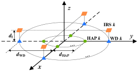
Figure 3: Simulation setup.

IV Simulation Results

As shown in Fig. 3, we consider a setup with $K=4$ pairs of HAPs and WDs, where HAP $k$ and WD $k$ are positioned in polar coordinates $\left(d_{\rm HAP},\frac{2\pi(k-1)}{K},\frac{\pi}{2}\right)$ and $\left(d_{\rm WD},\frac{2\pi(k-1)}{K},\frac{\pi}{2}\right)$ in meters (m), respectively. It is assumed that there are $L=K=4$ IRSs, with the $k$-th IRS located at a distance of $d_{\rm I}$ m directly above the $k$-th WD and equipped with $\frac{N}{4}$ elements. We adopt the distance-dependent path loss model and Rician fading channel model as detailed in [5]. The path loss is $-30$ dB at the reference distance of $1$ m, with the path loss exponents of $2.2$ for the IRS-related links and $3.5$ for the direct links. Moreover, the Rician factors of these two kinds of links are set to $3$ dB and $0$, respectively. Besides, we set $M=2$, $N=40$, $P_{i}=33$ dBm, $\sigma_{i}^{2}=-80$ dBm, $\forall i\in\mathcal{K}$, $T=1$ s, $\eta=0.7$, $d_{\rm WD}=7$ m, and $d_{\rm I}=2$ m, respectively.

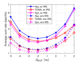
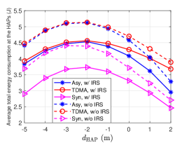
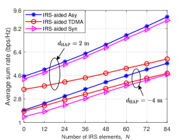
Figure 4: (a) Average sum throughput versus $d_{\rm HAP}$; (b) Average total energy consumption at the HAPs versus $d$; (c) Average sum throughput versus $N$.

In Fig. 4, we study the impact of cross-link channel power on the system performance in both cases with and without IRSs by varying the value of $d_{\rm HAP}$. Here, $d_{\rm HAP}<0$ means that HAP $k$ is located at $\left(-d_{\rm HAP},\frac{2\pi(k-1)}{K}+\pi,\frac{\pi}{2}\right)$ in m. First, it is observed that when $d_{\rm HAP}\geq-2$ m and increases, each scheme exhibits enhanced sum throughput performance. This can be attributed to the increased channel power of the direct links and reflected links (if present), which benefits both DL WPT and UL WIT. Second, when $d_{\rm HAP}\leq-2$ m and decreases, the sum throughputs of all the schemes increase. This is because the stronger cross-link channel power, although unfavorable for UL WIT, is advantageous for DL WPT, and these schemes can balance between DL WPT and UL WIT by optimizing the resource allocation to achieve better performance. Third, as expected, the Asy scheme consistently outperforms its sub-schemes, TDMA and Syn. Nevertheless, the performance gap between the Asy and Syn schemes decreases with the increase of $d_{\rm HAP}$. The reason is that the growing $d_{\rm HAP}$ results in reduced cross-link channel power, weakening the advantage of the Asy scheme in mitigating cross-link interference for more effective UL WIT through asymmetric time allocation and time-varying IRS beamforming (in the case with IRSs). Fourth, the Syn scheme gradually gains the upper hand over the TDMA scheme as $d_{\rm HAP}$ becomes large. This is because the performance gain brought by the TDMA scheme’s advantage of being free from cross-channel interference in UL WIT gradually decreases as $d_{\rm HAP}$ increases, ultimately dropping below the performance loss incurred due to the inefficient use of time resources. It is worth mentioning that integrating IRSs into the system also diminishes this advantage of the interference-free TDMA scheme, as the IRSs can assist the Asy and Syn schemes in more effectively mitigating cross-link interference. This is also why the introduction of IRSs widens the performance gap between the Asy and TDMA schemes and narrows the performance gap between the Syn and TDMA schemes in the presence of strong cross-link interference.

Next, we plot in Fig. 4 the total transmission energy consumption at the HAPs, denoted by $E_{\rm total}$, versus $d_{\rm HAP}$ for different schemes. Combining Figs. 4 and Fig. 4, we find that introducing IRSs into wireless powered communications in IFCs provides dual benefits, enhancing the system throughput while concomitantly reducing the total energy consumption at the HAPs. Besides, we note that the trends of the curves depicting the values of $E_{\rm total}$ are opposite to those of the curves illustrating the system sum throughputs. This is understandable since the value of $E_{\rm total}$ is proportional to the duration of DL WPT, and the system sum throughput is proportional to the duration of UL WIT, but the durations of DL WPT and UL WIT are inversely related.

Finally, Fig. 4 shows the average sum throughput versus $N$. It can be seen that in terms of the sum throughput gains achieved by increasing $N$, the TDMA scheme is evidently inferior to the Asy and Syn schemes. This is mainly because the increase in $N$ allows the Asy and Syn schemes to make better use of time resources to enhance performance, but it can hardly alleviate the performance bottleneck of the TDMA scheme caused by the waste of time resources. Moreover, from Figs. 4-4, we can find that although the Asy scheme always obtains the highest sum throughput, the other two schemes may be better choices in certain situations. Specifically, the TDMA scheme is preferable when the cross-link interference is overwhelming and $N$ is small, since its performance in sum throughput and energy cost approaches that of the Asy scheme in such cases and meanwhile it is easier to implement in practice. Additionally, the Syn scheme is more appealing when the cross-link interference is low, as it is not significantly inferior to the Asy scheme in terms of sum throughput performance while consuming less energy and being more practical to implement.

V Conclusion

In this paper, we proposed three transmission schemes, namely the IRS-aided Asy, TDMA, and Syn schemes, aiming to maximize the system sum throughput of a wireless powered IFC through resource allocation optimization. Despite the non-convexity of the three formulated problems, we proposed a general algorithmic framework applicable to solving each of them. Simulation results demonstrated the benefits of integrating IRSs into wireless powered IFCs in terms of both sum throughput performance and energy cost. We also drew useful insights into which scheme is the most attractive choice in certain scenarios, considering a comprehensive evaluation of performance and energy/implementation cost.

References

• [1] H. Ju and R. Zhang, “Throughput maximization in wireless powered communication networks,” IEEE Trans. Wireless Commun., vol. 13, no. 1, pp. 418–428, Jan. 2014.
• [2] L. Liu, R. Zhang, and K.-C. Chua, “Multi-antenna wireless powered communication with energy beamforming,” IEEE Trans. Commun., vol. 62, no. 12, pp. 4349–4361, Dec. 2014.
• [3] H. Lee, K.-J. Lee, H.-B. Kong, and I. Lee, “Sum-rate maximization for multiuser MIMO wireless powered communication networks,” IEEE Trans. Veh. Technol., vol. 65, no. 11, pp. 9420–9424, Nov. 2016.
• [4] H. Kim et al., “Sum-rate maximization methods for wirelessly powered communication networks in interference channels,” IEEE Trans. Wireless Commun., vol. 17, no. 10, pp. 6464–6474, Oct. 2018.
• [5] Q. Wu and R. Zhang, “Intelligent reflecting surface enhanced wireless network via joint active and passive beamforming,” IEEE Trans. Wireless Commun., vol. 18, no. 11, pp. 5394–5409, Nov. 2019.
• [6] Q. Wu, X. Zhou, and R. Schober, “IRS-assisted wireless powered NOMA: Do we really need different phase shifts in DL and UL?” IEEE Wireless Commun. Lett., vol. 10, no. 7, pp. 1493–1497, Jul. 2021.
• [7] X. Li, C. Zhang, C. He et al., “Sum-rate maximization in IRS-assisted wireless power communication networks,” IEEE Internet Things J., vol. 8, no. 19, pp. 14 959–14 970, Oct. 2021.
• [8] M. Hua and Q. Wu, “Throughput maximization for IRS-aided MIMO FD-WPCN with non-linear EH model,” IEEE J. Sel. Top. Signal Process., vol. 16, no. 5, pp. 918–932, Aug. 2022.
• [9] H. Yang, X. Chen, F. Yang et al., “Design of resistor-loaded reflectarray elements for both amplitude and phase control,” IEEE Antennas Wireless Propag. Lett., vol. 16, pp. 1159–1162, Nov. 2016.