Global Convergence of Natural Policy Gradient with Hessian-aided Momentum Variance Reduction

Abstract

Natural policy gradient (NPG) and its variants are widely-used policy search methods in reinforcement learning. Inspired by prior work, a new NPG variant coined NPG-HM is developed in this paper, which utilizes the Hessian-aided momentum technique for variance reduction, while the sub-problem is solved via the stochastic gradient descent method. It is shown that NPG-HM can achieve the global last iterate $\varepsilon$-optimality with a sample complexity of ${\cal O}(\varepsilon^{-2})$, which is the best known result for natural policy gradient type methods under the generic Fisher non-degenerate policy parameterizations. The convergence analysis is built upon a relaxed weak gradient dominance property tailored for NPG under the compatible function approximation framework, as well as a neat way to decompose the error when handling the sub-problem. Moreover, numerical experiments on Mujoco-based environments demonstrate the superior performance of NPG-HM over other state-of-the-art policy gradient methods.

1 Introduction

Reinforcement Learning (RL), which attempts to maximize long-term reward in a sequential decision-making task, has found a wide range of applications, for example in robotics [22], game playing [13], and recommendation systems [1]. A standard RL setting can be represented as a Markov Decision Process (MDP), denoted ${\cal M}=({\cal S},{\cal A},P,r,\gamma)$, where ${\cal S}$ is the state space, ${\cal A}$ is the action space, $P(s^{\prime}|s,a)$ denotes the probability of transitioning into state $s^{\prime}$ after taking action $a$ at state $s$, $r(s,a,s^{\prime})$ is the immediate reward, and $\gamma\in[0,1)$ is the discount factor. Assume the agent takes actions following a policy that is parameterized by a vector $\bm{\theta}\in\mathbb{R}^{d}$, denoted $\pi_{\bm{\theta}}:{\cal S}\to\Delta({\cal A})$. That is, at any time step $h$, the agent takes an action $a^{h}\sim\pi_{\bm{\theta}}(\cdot|s^{h})$, and then transitions to the next state $s^{h+1}\sim P(\cdot|s^{h},a^{h})$. In this paper we focus on the infinite horizon discounted setting. Given a trajectory $\tau=(s^{0},a^{0},r^{0},s^{1},a^{1},r^{1},\dots)$ induced by a policy $\pi_{\bm{\theta}}$, where $a^{h}\sim\pi_{\bm{\theta}}(\cdot|s^{h})$, $r^{h}=r(s^{h},a^{h},s^{h+1})$, and $s^{h+1}\sim P(\cdot|s^{h},a^{h})$, the state value function $V^{\pi_{\bm{\theta}}}:{\cal S}\to\mathbb{R}$ is defined as the average discounted sum of immediate rewards,

$$V^{\pi_{\bm{\theta}}}(s)=\mathbb{E}_{\tau}\left\{\sum_{h=0}^{\infty}\gamma^{h}r^{h}|s^{0}=s\rule{0.0pt}{8.53581pt}\right\}.$$ (1.1)

Under an initial state distribution $\rho$, the goal of RL is to find a parameter $\bm{\theta}$ that maximizes the expected cumulative rewards:

$$\max_{\bm{\theta}\in\mathbb{R}^{d}}\;J_{\rho}(\bm{\theta}):=\mathbb{E}_{s\sim\rho}\left\{V^{\pi_{\bm{\theta}}}(s)\rule{0.0pt}{8.53581pt}\right\}=\mathbb{E}_{\tau\sim p_{\bm{\theta}}}\left\{\sum_{h=0}^{\infty}\gamma^{h}r^{h}\rule{0.0pt}{8.53581pt}\right\},$$

where $p_{\bm{\theta}}$ denotes the trajectory distribution induced by $\pi_{\bm{\theta}}$:

$$p_{\bm{\theta}}(\tau)=\rho(s^{0})\prod_{h=0}^{\infty}\pi_{\bm{\theta}}(a^{h}|s^{h})P(s^{h+1}|s^{h},a^{h}).$$ (1.2)

Once RL is formulated as an optimization problem over the parameter space, a variety of optimization methods are available for seeking the optimal policy parameter, including vanilla policy gradient (PG), natural policy gradient (NPG) [19, 5], trust region policy optimization (TRPO) [41], proximal policy optimization (PPO) [42], actor-critics methods [23, 14, 36], and policy mirror ascent (PMA) [46, 24]. Compared with valued-based methods, policy optimization can be readily extended to high dimensional discrete or continuous action spaces via different parameterized policies, and is also amenable to a detailed analysis. Indeed, the convergence analyses of various policy optimization methods have received a lot of attention recently. We will first give a brief discussion towards this line of research.

1.1 Related works

Convergence of exact policy gradient methods.

Recently, a series of works have studied the global optimality (i.e., the convergence of $J_{\rho}(\bm{\theta}_{t})$ to $J_{\rho}^{*}$, where $\bm{\theta}_{t}$ is the output of an algorithm and $J_{\rho}^{*}$ is the optimal objective) of policy gradient methods when the policy gradient is exactly evaluated. Regarding the simplex parameterization, the sublinear convergence of the corresponding projected policy gradient (PPG) method with a constant step size has been investigated in [2, 55, 48, 26]. Furthermore, it can be shown that PPG is able to achieve the exact convergence in a finite number of iterations [26]. The sublinear convergence of the constant step size PG under the softmax parameterization (softmax PG) is established in [30, 29], where the linear convergence is further proved for the entropy-regularized softmax PG. Softmax NPG, a preconditioned version of softmax PG, also enjoys the sublinear convergence for a constant step size [2], while its local linear convergence is established in [20]. Moreover, a linear convergence rate for entropy-regularized softmax NPG is obtained in [8]. Noticing that softmax NPG in the policy space can be viewed as a special case of the policy mirror ascent method, the sublinear convergence can also be extended to the general PMA method with a constant step size [48]. In addition, the linear convergence of PMA has been established for geometrically increasing step sizes in the same work. Moreover, the convergence of PMA with different regularizers has been studied in [24, 54, 25].

Sample complexity for first-order stationary point convergence.

In practice, the policy gradient cannot be computed exactly, but should be estimated from random samples. Thus a line of research is devoted to the first-order stationary point analysis of policy optimization methods using sampled trajectories under general policy parameterizations, which follows closely the works in stochastic optimization. The vanilla PG is proved to require ${\cal O}(\varepsilon^{-4})$ random trajectories to reach an $\varepsilon$-stationary point such that $\|\nabla J_{\rho}(\bm{\theta}_{t})\|_{2}\leq\varepsilon$ [53, 27, 57, 38, 33]. Since the simple Monte Carlo estimate of policy gradient suffers from high variance, many variance reduction techniques have been introduced into PG to improve the sample efficiency and accelerate the algorithm, see for example [49, 51, 56, 12, 15, 40] and references therein. After the introduction of variance reduction, the sample complexity can be reduced from ${\cal O}(\varepsilon^{-4})$ to ${\cal O}(\varepsilon^{-3})$, which is overall optimal.

Sample complexity for global convergence.

There has been a surge of research studying the sample complexity of the sample-based policy gradient methods for the global convergence, which is also the focus of this paper. The property of gradient dominance, also known as Polyak-Lojasiewicz (PL) condition, is often used in this line of research. In a nutshell, gradient dominance prevents the gradient from vanishing unless reaching the global optimum. The sample-based NPG and Q-NPG methods under the log-linear policy have been studied within a compatible function approximation framework [2], establishing the ${\cal O}(\varepsilon^{-6})$ sample complexity through a connection between the global optimum and the update direction. This result has been improved to ${\cal O}(\varepsilon^{-2})$ for the geometrically increasing step sizes by viewing the sample-based NPG and Q-NPG methods as the approximate policy mirror optimization (APMO) methods [52]. Indeed, NPG performs intrinsically more and more akin to policy iteration with large enough learning rates, implying the geometric convergence. Moreover, the global convergence of APMO has been studied recently in [3] for the general Bregman projected policy and an ${\cal O}(\varepsilon^{-4})$ sample complexity is obtained for the special case of shallow neural network parameterization. For the general Fisher-non-degenerate policy, a relaxed weak gradient domination property is introduced in [10], and it is shown that momentum-based PG requires an ${\cal O}(\varepsilon^{-3})$ sample complexity to achieve the global average-regret convergence, defined as

$$J_{\rho}^{*}-\frac{1}{T}\sum^{T-1}_{t=0}\mathbb{E}\left\{J_{\rho}(\bm{\theta}_{t})\rule{0.0pt}{8.53581pt}\right\}\leq\varepsilon+{\cal O}(\sqrt{\varepsilon_{\mathrm{bias}}}),$$

where $\varepsilon_{\mathrm{bias}}$ is a parameter introduced in the compatible function approximation framework. Furthermore, the ${\cal O}(\varepsilon^{-3})$ sample complexity has been established in [53] for sample-based vanilla PG to achieve the global optimality of the form $\min_{t}\{J_{\rho}^{*}-\mathbb{E}\left\{J_{\rho}(\bm{\theta}_{t})\rule{0.0pt}{8.53581pt}\right\}\}\leq\varepsilon+{\cal O}(\sqrt{\varepsilon_{\mathrm{bias}}})$. In contrast, an (N)-HARPG method is proposed in [11] which only requires an ${\cal O}(\varepsilon^{-2})$ sample complexity to achieve the global last-iterate convergence, expressed as

$$J_{\rho}^{*}-\mathbb{E}\left\{J(\bm{\theta}_{T})\rule{0.0pt}{8.53581pt}\right\}\leq\varepsilon+{\cal O}(\sqrt{\varepsilon_{\mathrm{bias}}}).$$

An innovation in [11] is the Hessian-aided scheme for computing the gradient difference when constructing the moment-based variance reduction estimator, which can avoid the unverifiable assumption in the analysis when using importance sampling to construct the estimator. In addition, a double-loop variance-reduced NPG with batch gradients is proposed in [27] and the ${\cal O}(\varepsilon^{-3})$ sample complexity for the global average-regret convergence has been established. This sample complexity has been improved to ${\cal O}(\varepsilon^{-2})$ for accelerated natural policy gradient (ANPG) [31], in which an accelerated gradient descent procedure is utilized to solve the sub-problem concerning the NPG update direction.

1.2 Main contributions

The main contributions of this paper are summarized as follows:

• Inspired by [11], a sample-based natural policy gradient method with Hessian-aided momentum variance reduction (NPG-HM) is proposed. Compared with the variance reduction NPG method developed in [27], NPG-HM is a single-loop algorithm that avoids the usage of importance sampling when constructing the unbiased policy gradient estimator. Numerical experiments on Mujoco-based environments demonstrate that NPG-HM outperforms the other state-of-the-art policy gradient methods.

• The global convergence of NPG-HM is studied when the sub-problem for computing the NPG update direction is solved via the stochastic gradient descent method. It is shown that it requires an ${\cal O}(\varepsilon^{-2})$ sample complexity for NPG-HM to achieve the global last-iterate $\varepsilon$-optimality under the general Fisher-non-degenerate policy, differing from the average-regret convergence results established in [27] and [31] for sample-based NPG methods. Though our analysis is also inspired by [11], the extension is by no means trivial since it involves solving a sub-problem through SGD in NPG-HM. More precisely, an innovative way to decompose the error is used when handling the sub-problem, and then a recursive sequence is developed based on the decomposition, see Lemma 4.8 and Lemma 4.10, respectively. A comparison with other sample-based PG and NPG methods which also enjoy global convergence is presented in Table 1.

Table 1: Sample complexities of sample-based PG and NPG methods to achieve a global $\varepsilon$-optimality. “IS-free” means the importance sampling technique is not required, while “Last-iterate” indicates the global last-iterate convergence.

Algorithm	Parameterization	Sample Complexity	IS-free	Last-iterate
NPG [2]	Log-linear	$\varepsilon^{-6}$	✓	✗
NPG [52]	Log-linear	$\varepsilon^{-2}$	✓	✓
PG  [53]	Fisher-non-degenerate	$\varepsilon^{-3}$	✓	✗
STORM-PG  [10]	Fisher-non-degenerate	$\varepsilon^{-3}$	✗	✗
(N)-HARPG [11]	Fisher-non-degenerate	$\varepsilon^{-2}$	✓	✓
NPG-SRVR [27]	Fisher-non-degenerate	$\varepsilon^{-2.5}+\varepsilon^{-3}$	✗	✗
ANPG  [31]	Fisher-non-degenerate	$\varepsilon^{-2}$	✓	✗
NPG-HM	Fisher-non-degenerate	$\varepsilon^{-2}$	✓	✓

1.3 Paper organization

The rest of this paper is organized as follows. In Section 2, we review some results and methods about RL and variance reduction. The description of the proposed NPG-HM and the main theoretical result is presented in Section 3. The proof of the main result is provided in Section 4. Numerical experiments conducted to compare NPG-HM with other policy gradient methods can be found in Section 5. In Section 6, we conclude this paper with a few interesting future research directions. Finally, Section 7 is devoted to the proofs of some technical lemmas.

2 Preliminaries

Recalling the definition of state value function in (1.1), there are another two value functions which are closely related. Given a state-action pair $(s,a)$, define the state-action value function (or Q-function) $Q^{\pi_{\bm{\theta}}}:{\cal S}\times{\cal A}\to\mathbb{R}$ as follows:

$$Q^{\pi_{\bm{\theta}}}(s,a)=\mathbb{E}_{\tau}\left\{\sum_{h=0}^{\infty}\gamma^{h}r^{h}|s^{0}=s,a^{0}=a\rule{0.0pt}{8.53581pt}\right\}.$$

It is easy to show that

$$V^{\pi_{\bm{\theta}}}(s)=\mathbb{E}_{a\sim\pi_{\bm{\theta}}(\cdot|s)}\left\{Q^{\pi_{\bm{\theta}}}(s,a)\rule{0.0pt}{8.53581pt}\right\}.$$

In addition, the advantage function $A^{\pi_{\bm{\theta}}}:{\cal S}\times{\cal A}\to\mathbb{R}$ which measures how well a single action $a$ behaves compared with the average value is defined as

$$A^{\pi_{\bm{\theta}}}(s,a)=Q^{\pi_{\bm{\theta}}}(s,a)-V^{\pi_{\bm{\theta}}}(s).$$

2.1 Policy gradient

Define the state visitation distribution $d_{\rho,\pi_{\bm{\theta}}}$ induced by policy $\pi_{\bm{\theta}}$ as

$$d_{\rho,\pi_{\bm{\theta}}}(s)=(1-\gamma)\mathbb{E}_{s^{0}\sim\rho}\left\{\sum_{h=0}^{\infty}\gamma^{h}\mathbb{P}\left\{s^{h}=s|s^{0},\pi_{\bm{\theta}}\rule{0.0pt}{8.53581pt}\right\}\rule{0.0pt}{8.53581pt}\right\},$$

where $\mathbb{P}\left\{s^{h}=s|s^{0},\pi_{\bm{\theta}}\rule{0.0pt}{8.53581pt}\right\}$ is the probability that the state $s$ is visited at time step $h$, given that the trajectory starts from $s^{0}$ and follows policy $\pi_{\bm{\theta}}$. Moreover, define the state-action visitation distribution $\tilde{d}_{\rho,\pi_{\bm{\theta}}}(s,a)$ as

$$\tilde{d}_{\rho,\pi_{\bm{\theta}}}(s,a)=d_{\rho,\pi_{\bm{\theta}}}(s)\cdot\pi_{\bm{\theta}}(a|s).$$ (2.1)

Then the policy gradient of $J_{\rho}(\bm{\theta})$ with respect to $\bm{\theta}$ can be expressed as ([44])

$$\nabla J_{\rho}(\bm{\theta}) =\frac{1}{1-\gamma}\mathbb{E}_{(s,a)\sim\tilde{d}_{\rho,\pi_{\bm{\theta}}}}\left\{\nabla\log\pi_{\bm{\theta}}(a|s)Q^{\pi_{\bm{\theta}}}(s,a)\rule{0.0pt}{8.53581pt}\right\}$$

$$=\frac{1}{1-\gamma}\mathbb{E}_{(s,a)\sim\tilde{d}_{\rho,\pi_{\bm{\theta}}}}\left\{\nabla\log\pi_{\bm{\theta}}(a|s)A^{\pi_{\bm{\theta}}}(s,a)\rule{0.0pt}{8.53581pt}\right\},$$

where the second equality relies on the assumption $\sum_{a\in\mathcal{A}}\pi_{\bm{\theta}}(a|s)=1,\forall\,\bm{\theta}\in\mathbb{R}^{d}$ that will be made throughout this paper. In terms of the expectation with respect to the trajectory, $\nabla J_{\rho}(\bm{\theta})$ has the following alternative expression:

$$\nabla J_{\rho}(\bm{\theta})=\mathbb{E}_{\tau\sim p_{\bm{\theta}}}\left\{\sum_{h=0}^{\infty}\left(\sum_{i=h}^{\infty}\gamma^{i}r^{i}\right)\nabla\log\pi_{\bm{\theta}}(a^{h}|s^{h})\rule{0.0pt}{8.53581pt}\right\},$$ (2.2)

where $p_{\bm{\theta}}$ is given in (1.2). In addition, the policy Hessian $\nabla^{2}J(\bm{\theta})$ which will be used later is given by ([43])

$$\nabla^{2}J_{\rho}(\bm{\theta})=\mathbb{E}_{\tau\sim p_{\bm{\theta}}}\left\{\nabla\phi(\tau;\bm{\theta})(\nabla\log p_{\bm{\theta}}(\tau))^{\mathsf{T}}+\nabla^{2}\phi(\tau;\bm{\theta})\rule{0.0pt}{8.53581pt}\right\},$$ (2.3)

where $\phi(\tau;{\bm{\theta}})=\sum_{h=0}^{\infty}\left(\sum_{i=h}^{\infty}\gamma^{i}r^{i}\right)\log\pi_{\bm{\theta}}(a^{h}|s^{h})$.

Given the expression of policy gradient, the vanilla policy gradient method simply updates the policy parameter along the gradient ascent direction:

$$\bm{\theta}_{t+1}=\bm{\theta}_{t}+\alpha_{t}\nabla J_{\rho}(\bm{\theta}_{t}),$$

where $\alpha_{t}$ is the learning rate. As previously mentioned, the policy gradient needs to be estimated from random samples in practice. The expression in (2.2) provides a natural unbiased estimator based on random trajectories. However, the length of sampled trajectories cannot be infinite in practice. Thus we instead consider the following truncated estimator:

$$\bm{g}(\tau;\bm{\theta}):=\sum_{h=0}^{H-1}\left(\sum_{i=h}^{H-1}\gamma^{i}r^{i}\right)\nabla\log\pi_{\bm{\theta}}(a^{h}|s^{h}).$$ (2.4)

Note that $\bm{g}(\tau;\bm{\theta})$ is a biased estimator for $\nabla J_{\rho}(\bm{\theta})$, but an unbiased estimator for $\nabla J_{\rho}^{H}(\bm{\theta})$, where

$$J_{\rho}^{H}(\bm{\theta})=\mathbb{E}_{\tau\sim p_{\bm{\theta}}}\left\{\sum_{h=0}^{H-1}\gamma^{h}r^{h}\rule{0.0pt}{8.53581pt}\right\},$$

with

$$p_{\bm{\theta}}(\tau)=\rho(s^{0})\prod_{h=0}^{H-1}\pi_{\bm{\theta}}(a^{h}|s^{h})P(s^{h+1}|s^{h},a^{h}).$$ (2.5)

Similarly, we will consider the following truncated and biased estimator for $\nabla^{2}J(\bm{\theta})$:

$$\bm{H}(\tau;\bm{\theta}):=\nabla\phi(\tau;\bm{\theta})(\nabla\log p_{\bm{\theta}}(\tau))^{\mathsf{T}}+\nabla^{2}\phi(\tau;\bm{\theta}),$$ (2.6)

where $\phi(\tau;{\bm{\theta}})=\sum_{h=0}^{H-1}\left(\sum_{i=h}^{H-1}\gamma^{i}r^{i}\right)\log\pi_{\bm{\theta}}(a^{h}|s^{h})$, which again is an unbiased estimator for $\nabla^{2}J^{H}_{\rho}(\bm{\theta})$.

2.2 Natural policy gradient

As an important variant of PG, NPG utilizes the Fisher Information Matrix (FIM) as a preconditioner to refine the gradient direction based on the underlying structure of the parameterized policy space, which can be approximately viewed as a second-order method. The FIM $\bm{F}(\bm{\theta})$ is defined by

$$\bm{F}(\bm{\theta})=\mathbb{E}_{(s,a)\sim\tilde{d}_{\rho,\pi_{\bm{\theta}}}}\left\{\nabla\log\pi_{\bm{\theta}}(a|s)\left(\nabla\log\pi_{\bm{\theta}}(a|s)\right)^{\mathsf{T}}\rule{0.0pt}{8.53581pt}\right\},$$ (2.7)

where $\tilde{d}_{\rho,\pi_{\bm{\theta}}}$ represents the state-action visitation distribution defined in (2.1). Given the FIM, the NPG update takes the following form:

$$\bm{\theta}_{t+1}=\bm{\theta}_{t}+\alpha_{t}\bm{F}^{\dagger}(\bm{\theta}_{t})\nabla J_{\rho}(\bm{\theta}_{t}),$$ (2.8)

where $\alpha_{t}$ is the learning rate, and $\bm{F}^{\dagger}(\bm{\theta})$ is the Moore-Penrose pseudoinverse of $\bm{F}(\bm{\theta})$.

Moreover, for any $\bm{\theta}$ and $\bm{w}$, define the compatible function approximation error as follows:

$$L(\bm{w};\bm{\theta})=\frac{1}{2}\mathbb{E}_{(s,a)\sim\tilde{d}_{\rho,\pi_{\bm{\theta}}}}\left\{\left((1-\gamma)\bm{w}^{\top}\nabla\log\pi_{\bm{\theta}}(a|s)-A^{\pi_{\bm{\theta}}}(s,a)\right)^{2}\rule{0.0pt}{8.53581pt}\right\}.$$ (2.9)

Then it is easy to see that $\bm{w}_{t}^{\ast}=\bm{F}^{\dagger}(\bm{\theta}_{t})\nabla J_{\rho}(\bm{\theta}_{t})$ is a minimizer of (2.9). Thus, the NPG update direction can be obtained by solving the following minimization problem:

$$\bm{w}_{t}^{\ast}=\operatorname*{arg\,min}_{\bm{w}}L(\bm{w};\bm{\theta}_{t}).$$

It is also evident that $\bm{w}_{t}^{\ast}$ is a minimizer of

$$\min_{\bm{w}\in\mathbb{R}^{d}}\left\{\frac{1}{2}\mathbb{E}_{(s,a)\sim\tilde{d}_{\rho,\pi_{\bm{\theta}_{t}}}}\left\{\left(\bm{w}^{\top}\nabla\log\pi_{\bm{\theta}_{t}}(a|s)\right)^{2}\rule{0.0pt}{8.53581pt}\right\}-\bm{w}^{\mathsf{T}}\nabla J_{\rho}(\bm{\theta}_{t})\right\}.$$ (2.10)

2.3 Hessian-aided momentum variance reduction

Recall that the momentum-based gradient estimator from [10, 15] is given by

$$\bm{v}_{t}=\beta_{t}\bm{g}(\tau_{t};\bm{\theta}_{t})+(1-\beta_{t})\left(\bm{v}_{t-1}+\bm{g}(\tau_{t};\bm{\theta}_{t})-\omega(\tau_{t}|\bm{\theta}_{t-1},\bm{\theta}_{t})\cdot\bm{g}(\tau_{t};\bm{\theta}_{t-1})\right),$$ (2.11)

where $\beta_{t}\in(0,1]$ is the momentum coefficient, and $\omega(\tau_{t}|\bm{\theta}_{t-1},\bm{\theta}_{t})$ is the importance sampling weight:

$$\omega(\tau_{t}|\bm{\theta}_{t-1},\bm{\theta}_{t})=\frac{p_{\bm{\theta}_{t-1}}(\tau_{t})}{p_{\bm{\theta}_{t}}(\tau_{t})}=\prod_{h=0}^{H-1}\frac{\pi_{\bm{\theta}_{t-1}}(a^{h}|s^{h})}{\pi_{\bm{\theta}_{t}}(a^{h}|s^{h})}.$$ (2.12)

Here the importance sampling weight is introduced to guarantee that $\bm{g}(\tau_{t};\bm{\theta}_{t})-\omega(\tau_{t}|\bm{\theta}_{t-1},\bm{\theta}_{t})\cdot\bm{g}(\tau_{t};\bm{\theta}_{t-1})$ is an unbiased estimator of the gradient difference $\nabla J_{\rho}^{H}(\bm{\theta}_{t})-\nabla J_{\rho}^{H}(\bm{\theta}_{t-1})$, i.e.,

$$\mathbb{E}_{\tau_{t}}\left\{\bm{g}(\tau_{t};\bm{\theta}_{t})-\omega(\tau_{t}|\bm{\theta}_{t-1},\bm{\theta}_{t})\cdot\bm{g}(\tau_{t};\bm{\theta}_{t-1})\rule{0.0pt}{8.53581pt}\right\}=\nabla J_{\rho}^{H}(\bm{\theta}_{t})-\nabla J_{\rho}^{H}(\bm{\theta}_{t-1}).$$

The momentum-based method combines the unbiased SGD estimator [6] with the SARAH estimator [32] under a single-loop framework, which can avoid the high computational cost in variance reduction.

Note, however, that the existence of the importance sampling weight requires a strong unverifiable assumption for the convergence analysis of the corresponding method. In order to handle this issue, a Hessian-aided momentum-based estimator is proposed in [11, 39]. The main idea is to construct an unbiased estimate of $\nabla J_{\rho}^{H}({\bm{\theta}}_{t})-\nabla J_{\rho}^{H}({\bm{\theta}}_{t-1})$ using the integral of policy Hessian. Let $\hat{\bm{\theta}}_{t}$ be a linear combination of $\bm{\theta}_{t}$ and $\bm{\theta}_{t-1}$,

$$\hat{\bm{\theta}}_{t}=q\bm{\theta}_{t}+(1-q)\bm{\theta}_{t-1},$$ (2.13)

where $q$ obeys the uniform distribution over $[0,1]$, denoted $\operatorname{Unif}(0,1)$. Let $\hat{\tau}_{t}$ be a trajectory generated by the policy $\pi_{\hat{\bm{\theta}}_{t}}$, and $\bm{H}(\hat{\tau}_{t};\hat{\bm{\theta}}_{t})$ be an unbiased estimate of policy Hessian $\nabla^{2}J_{\rho}^{H}(\hat{\bm{\theta}}_{t})$. A simple calculation yields that

$$\nabla J_{\rho}^{H}(\bm{\theta}_{t})-\nabla J_{\rho}^{H}(\bm{\theta}_{t-1}) =\int_{0}^{1}\nabla^{2}J_{\rho}^{H}\left(q\bm{\theta}_{t}+(1-q)\bm{\theta}_{t-1}\right)(\bm{\theta}_{t}-\bm{\theta}_{t-1})dq$$

$$=\mathbb{E}_{q}\left\{\nabla^{2}J_{\rho}^{H}(\hat{\bm{\theta}}_{t})(\bm{\theta}_{t}-\bm{\theta}_{t-1})\rule{0.0pt}{8.53581pt}\right\}$$

$$=\mathbb{E}_{q}\left\{\mathbb{E}_{\hat{\tau}_{t}}\left\{\bm{H}(\hat{\tau}_{t};\hat{\bm{\theta}}_{t})(\bm{\theta}_{t}-\bm{\theta}_{t-1})\rule{0.0pt}{8.53581pt}\right\}\bigg{|}q\rule{0.0pt}{8.53581pt}\right\}$$

$$=\mathbb{E}\left\{\bm{H}(\hat{\tau}_{t};\hat{\bm{\theta}}_{t})(\bm{\theta}_{t}-\bm{\theta}_{t-1})\rule{0.0pt}{8.53581pt}\right\},$$

which implies that $\bm{H}(\hat{\tau}_{t};\hat{\bm{\theta}}_{t})(\bm{\theta}_{t}-\bm{\theta}_{t-1})$ is an unbiased estimator of $\nabla J_{\rho}^{H}({\bm{\theta}}_{t})-\nabla J_{\rho}^{H}({\bm{\theta}}_{t-1})$. Based on this observation, the Hessian-aided momentum-based estimator is given by

$$\bm{u}_{t}=\beta_{t}\bm{g}(\tau_{t};\bm{\theta}_{t})+(1-\beta_{t})\left(\bm{u}_{t-1}+\bm{H}(\hat{\tau}_{t};\hat{\bm{\theta}}_{t})(\bm{\theta}_{t}-\bm{\theta}_{t-1})\right),$$ (2.14)

where $\tau_{t}\sim p_{\bm{\theta}_{t}},\hat{\tau}_{t}\sim p_{\hat{\bm{\theta}}_{t}}$, and the momentum coefficient $\beta_{t}$ is time-varying.

3 NPG-HM and Its Global Convergence

3.1 NPG-HM

As already mentioned, NPG-HM is a sample-based NPG with Hessian-aided momentum variance reduction. A detailed description of the method is presented in Algorithm 1. More concretely, the estimates of policy gradient and Hessian are calculated using the expressions (2.4) and (2.6), respectively. The unbiased estimator of policy gradient is calculated using (2.14), see line 7 of Algorithm 1. As is pointed out in [11], the Hessian-vector product in line 7 can be efficiently computed as follows:

$$\bm{H}(\hat{\tau}_{t};\hat{\bm{\theta}}_{t})\bm{x}=\left\langle\nabla\log p_{\hat{\bm{\theta}}_{t}}(\hat{\tau}_{t}),\bm{x}\right\rangle\bm{g}(\hat{\tau}_{t};\hat{\bm{\theta}}_{t})+\nabla\left\langle\bm{g}(\hat{\tau}_{t};\hat{\bm{\theta}}_{t}),\bm{x}\right\rangle,$$

where $\bm{x}\in\mathbb{R}^{d}$ is an arbitrary vector. In line 9, the update direction $\bm{w}_{t}$ is generated by NPG-SGD (see Algorithm 2), which applies the SGD method to solve the following sub-problem:

$$\min_{\bm{w}\in\mathbb{R}^{d}}\left\{\frac{1}{2}\mathbb{E}_{(s,a)\sim\tilde{d}_{\rho,\pi_{\bm{\theta}_{t}}}}\left\{\left(\bm{w}^{\top}\nabla\log\pi_{\bm{\theta}_{t}}(a|s)\right)^{2}\rule{0.0pt}{8.53581pt}\right\}-\bm{w}^{\mathsf{T}}\bm{u}_{t}\right\}.$$ (3.1)

Since $\bm{u}_{t}$ is an unbiased estimator of $\nabla J_{\rho}(\bm{\theta}_{t})$, the update direction $\bm{w}_{t}$ can be regarded as an approximation of $\bm{w}_{t}^{\ast}$ by noting (2.10).

Input: Number of iterations $T$, horizon $H$, and initial parameter ${\bm{\theta}}_{1}\in\mathbb{R}^{d}$

1 for $t=1,2,\cdots,T-1$ do

2       if $t=1$ then

3             Sample a trajectory $\tau_{1}$ from $p_{\bm{\theta}_{1}}$ and compute $\bm{u}_{1}=\bm{g}(\tau_{1};\bm{\theta}_{1})$;

4            

5      else

6            

7            Sample $q_{t}$ from $\operatorname{Unif}(0,1)$ and calculate $\hat{\bm{\theta}}_{t}=q_{t}\bm{\theta}_{t}+(1-q_{t})\bm{\theta}_{t-1}$;

8            

9            Sample two trajectories $\tau_{t}$ and $\hat{\tau}_{t}$ from $p_{\bm{\theta}_{t}}$ and $p_{\hat{\bm{\theta}}_{t}}$, respectively;

10            

11            Calculate

$$\bm{u}_{t}=\beta_{t}\bm{g}(\tau_{t};\bm{\theta}_{t})+(1-\beta_{t})\left(\bm{u}_{t-1}+\bm{H}(\hat{\tau}_{t};\hat{\bm{\theta}}_{t})(\bm{\theta}_{t}-\bm{\theta}_{t-1})\right)$$

with $\beta_{t}=20/(t+20)$ ;

12            

13       end if

14      

15      $\bm{w}_{t}=\text{NPG-SGD}(\tilde{d}_{\rho,\pi_{\bm{\theta}_{t}}},\pi_{\bm{\theta}_{t}},\bm{u}_{t})$;

16      

17      $\bm{\theta}_{t+1}=\bm{\theta}_{t}+\alpha_{t}\bm{w}_{t}$ with $\alpha_{t}=\alpha_{0}\beta_{t}^{1/2}$;

18      

19 end for

20

Output: $\bm{\theta}_{T}$

Algorithm 1 Natural Policy Gradient with Hessian-aided Momentum (NPG-HM)

Input: Distribution $\tilde{d}_{\rho,\pi_{\bm{\theta}}}$, policy $\pi_{\bm{\theta}}$, gradient estimate $\bm{u}$, and initial parameter $\bm{w}^{0}\in\mathbb{R}^{d}$

1

2for $k=0,\cdots,K-1$ do

3       Sample a state-action pair $(s_{k},a_{k})$ from $\tilde{d}_{\rho,\pi_{\bm{\theta}}}$;

4       Calculate

$$\bm{w}^{k+1}=\bm{w}^{k}-\eta\left(\left({\bm{w}^{k}}^{\mathsf{T}}\nabla\log\pi_{\bm{\theta}}(a_{k}|s_{k})\right)\nabla\log\pi_{\bm{\theta}}(a_{k}|s_{k})-\bm{u}\right)$$

with $\eta=1/(4M_{g})$;

5      

6 end for

7

Output: $\bm{w}_{t}=\frac{1}{K+1}\sum_{k=0}^{K}\bm{w}^{k}$

Algorithm 2 NPG-SGD

3.2 Global convergence of NPG-HM

In this section, we present the global convergence of NPG-HM for the Fisher-non-degenerate policy class given in Definition 3.1. Another two standard and useful assumptions, Assumptions 3.1 and 3.2, will also be first introduced. It is worth noting that Definition 3.1, Assumption 3.1, and Assumption 3.2 can be satisfied by certain Gaussian policies. We refer interested readers to [34, 49, 11, 27] for more details.

Definition 3.1.

For an initial distribution $\rho$, a policy $\pi_{\bm{\theta}}$ with $\bm{\theta}\in\mathbb{R}^{d}$ is considered to be Fisher-non-degenerate if there exists a positive constant $\mu_{F}$ such that the Fisher Information Matrix (FIM) $\bm{F}(\bm{\theta})$ induced by $\pi_{\bm{\theta}}$ and $\rho$ (see (2.7)) satisfies $\bm{F}(\bm{\theta})\succcurlyeq\mu_{F}\bm{I}_{d}$.

Assumption 3.1.

Let $\pi_{\bm{\theta}}$ be the policy parameterized by $\bm{\theta}\in\mathbb{R}^{d}$. There exist constants $M_{g},M_{h}>0$ such that the gradient and Hessian of the log-density of the policy satisfy

$$\|\nabla\log\pi_{\bm{\theta}}(a|s)\|_{2}^{2}\leq M_{g}\text{ and }\|\nabla^{2}\log\pi_{\bm{\theta}}(a|s)\|_{2}\leq M_{h}$$

for any $a\in{\cal A}$ and $s\in{\cal S}$.

Remark 3.1.

Note that Assumption 3.1 is generic and standard for convergence analysis of policy gradient methods, see [34, 49, 15, 11]. Moreover, based on Definition 3.1 and Assumption 3.1, we can easily conclude that

$$\mu_{F}\bm{I}\preccurlyeq\bm{F}(\bm{\theta})\preccurlyeq M_{g}\bm{I}.$$

In the sequel, we will let $\kappa=M_{g}/\mu_{F}$.

As the class of Fisher-non-degenerate policies may not encompass all stochastic policies, we will utilize the framework of compatible function approximation error, see [2, 10, 27, 11], to reflect the expressiveness of the policy class.

Assumption 3.2.

For any policy $\pi_{\bm{\theta}}$ with some $\bm{\theta}$, there exists a positive constant $\varepsilon_{\operatorname{bias}}$ such that

$$\mathbb{E}_{(s,a)\sim\tilde{d}_{\rho,\pi^{\ast}}}\left\{\left(A^{\pi_{\bm{\theta}}}(s,a)-(1-\gamma)(w^{\ast}_{\bm{\theta}})^{\mathsf{T}}\nabla\log\pi_{\bm{\theta}}(a|s)\right)^{2}\rule{0.0pt}{8.53581pt}\right\}\leq\varepsilon_{\mathrm{bias}},$$ (3.2)

where $\tilde{d}_{\rho,\pi\ast}(s,a)=d_{\rho,\pi^{\ast}}(s)\cdot\pi^{\ast}(a|s)$ is the state-action distribution induced by an optimal policy $\pi^{\ast}$ that maximizes $J_{\rho}(\pi)=\mathbb{E}_{s^{0}\sim\rho}\left\{V^{\pi}(s^{0})\rule{0.0pt}{8.53581pt}\right\}$, and $\bm{w}^{\ast}_{\bm{\theta}}=\bm{F}^{-1}(\bm{\theta})\nabla J_{\rho}(\bm{\theta})$ is the exact NPG update direction at $\bm{\theta}$.

Remark 3.2.

Assumption 3.2 states that the advantage function, denoted by $A^{\pi_{\bm{\theta}}}(s,a)$, can be effectively approximated using the score function $\nabla\log\pi_{\bm{\theta}}(a|s)$. Previous works have already established that $\varepsilon_{\operatorname{bias}}$ is zero for the tabular softmax parameterization policy [2] or the underlying MDP exhibiting a specific low-rank structure [16, 50, 17]. Furthermore, if the policy is parameterized using a neural network, $\varepsilon_{\mathrm{bias}}$ can be exceedingly small [47].

Theorem 3.1.

Suppose $H=-\frac{1}{\log\gamma}\log(T+\tau_{0}),\beta_{t}=\frac{\tau_{0}}{t+\tau_{0}},\alpha_{t}=\alpha_{0}\beta_{t}^{1/2},\lambda_{t}=\lambda_{0}\beta_{t}^{-1/2},\lambda_{0}=\frac{\kappa\tau_{0}\alpha_{0}}{4\mu_{F}}$ and $\alpha_{0}=\sqrt{\frac{\mu_{F}^{2}}{\kappa\tau_{0}(12L^{2}+6\nu_{h}^{2})}}$, where $t\geq 1$ and $\tau_{0}\geq 20$. Assume NPG-SGD, see Algorithm 2, is run $K$ iterations to obtain an update direction with $K\geq 48\kappa^{4}(\sqrt{2d}+1)^{2}$. Let $\bm{\theta}_{1}$ be the initialization. Then the output $\bm{\theta}_{T}$ of Algorithm 1 obeys that

$$\mathbb{E}\left\{J_{\rho}^{\ast}-J_{\rho}(\bm{\theta}_{T})\rule{0.0pt}{8.53581pt}\right\} \lesssim\frac{\mathbb{E}\left\{J_{\rho}^{\ast}-J_{\rho}(\bm{\theta}_{1})\rule{0.0pt}{8.53581pt}\right\}}{T^{2}}+\frac{\nu_{g}^{2}}{T^{2}}+\frac{\kappa^{3/2}}{1-\frac{\kappa^{4}d}{K}}\frac{1}{\sqrt{T}}+\frac{1}{T^{3/2}}+\frac{\sqrt{\varepsilon_{\operatorname{bias}}}}{1-\gamma}.$$

Remark 3.3.

Theorem 3.1 shows that NPG-HM enjoys an ${\cal O}(\varepsilon^{-2})$ sample complexity to achieve the global last-iterate convergence. Note that the establishment of this result closely relies on the fact that it suffices to run the sub-problem solver (i.e., Algorithm 2) for a constant number of iterations ( i.e., the value of $K$ is independent of $\varepsilon$ to achieve $\mathbb{E}\left\{J_{\rho}^{\ast}-J_{\rho}(\bm{\theta}_{T})\rule{0.0pt}{8.53581pt}\right\}\lesssim\varepsilon$). This is indeed the key for us to be able to establish the ${\cal O}(\varepsilon^{-2})$ sample complexity. In addition, a similar result can be established if we replace the gradient estimator in NPG-HM (line 7 of Algorithm 1) by the one based on importance sampling, i.e., the one in (2.11). However, as already stated, the analysis will then require an assumption on the importance sampling weight that is difficult to check. The details are omitted.

4 Proof of Main Theorem

We first list some useful lemmas that will be used in the proof of Theorem 3.1. In particular, a new relaxed weak gradient dominance property and a novel ascent lemma are established, see Lemma 4.6 and Lemma 4.7, respectively. Moreover, the sample complexity of the subroutine (Algorithm 2) in NPG-HM is carefully analyzed via an innovative error decomposition, see Lemma 4.8. Then a recursive sequence is developed in Lemma 4.10. The proofs of Lemmas 4.5-4.10 are delayed to Section 7.

Lemma 4.1.

Under Assumption 3.1, for all $\bm{\theta}\in\mathbb{R}^{d}$, one has

• $J_{\rho}(\bm{\theta})$ is $L$-smooth, where $L=\frac{1}{(1-\gamma)^{2}}(M_{g}+M_{h})$,

• $J_{\rho}^{H}(\bm{\theta})$ is $L$-smooth, where $L=\frac{1}{(1-\gamma)^{2}}(M_{g}+M_{h})$,

• $\max\left\{\left\|\nabla J_{\rho}^{H}(\bm{\theta})\right\|_{{\footnotesize{2}}},\left\|\nabla J_{\rho}(\bm{\theta})\right\|_{{\footnotesize{2}}}\right\}\leq\frac{\sqrt{M_{g}}}{(1-\gamma)^{3/2}}$.

Remark 4.1.

The first result can be found in [53, Lemma 4.4], which improves the results in [49, 27, 35]. For the second one, the smoothness with a constant $L=\frac{M_{h}}{(1-\gamma)^{2}}+\frac{2M_{g}}{(1-\gamma)^{3}}$ is established in [49, Proposition 4.2]. However, following a similar argument for the non-truncated objective (i.e. proof for the first result in [53, Lemma 4.4]), it is evident that the constant can be improved to $L=\frac{1}{(1-\gamma)^{2}}(M_{g}+M_{h})$. The last one can be found in [53, Lemma D.1], which improves the results in [49, 27, 35].

Lemma 4.2.

Let $\bm{g}(\tau;\bm{\theta})$ and $\bm{H}(\tau;\bm{\theta})$ be the unbiased estimates of policy gradient $\nabla J_{\rho}^{H}(\bm{\theta})$ and policy Hessian $\nabla^{2}J_{\rho}^{H}(\bm{\theta})$, respectively. Under Assumption 3.1 and the fact that $r(s,a,s^{\prime})\in[-1,1]$, one has

$$\mathbb{E}_{\tau}\left\{\left\|\bm{g}(\tau;\bm{\theta})-\nabla J^{H}_{\rho}(\bm{\theta})\right\|_{{\footnotesize{2}}}^{2}\rule{0.0pt}{8.53581pt}\right\} \leq\mathbb{E}_{\tau}\left\{\left\|\bm{g}(\tau;\bm{\theta})\right\|_{{\footnotesize{2}}}^{2}\rule{0.0pt}{8.53581pt}\right\}\leq\nu_{g}^{2},$$ (4.1)

$$\mathbb{E}_{\tau}\left\{\left\|\bm{H}(\tau;\bm{\theta})\right\|^{2}\rule{0.0pt}{8.53581pt}\right\} \leq\nu_{h}^{2},$$ (4.2)

where $\nu_{g}^{2}=\frac{M_{g}}{(1-\gamma)^{3}}$ and $\nu_{h}^{2}=\frac{2H^{2}M_{g}^{2}}{(1-\gamma)^{3}}+\frac{2M_{h}^{2}}{(1-\gamma)^{4}}$, and $\|\cdot\|$ is referred to as the spectral norm of a matrix.

Remark 4.2.

The variance of the gradient estimator is provided in [53, Lemma 4.2], which improves the results in [43, 37, 35]. In [43, Lemma 4.1], an upper bound of $\mathbb{E}_{\tau}\left\{\left\|\bm{H}(\tau;\bm{\theta})\right\|^{2}\rule{0.0pt}{8.53581pt}\right\}$ with $\nu_{h}^{2}=\frac{2H^{2}M_{g}^{2}+2M_{h}^{2}}{(1-\gamma)^{4}}$ is established. However, based a better bound for $\mathbb{E}_{\tau}\left\{\left\|\bm{g}(\tau;\bm{\theta})\right\|_{{\footnotesize{2}}}^{2}\rule{0.0pt}{8.53581pt}\right\}$ (i.e., Equation (4.1)), it is easy to see that $\nu_{h}^{2}$ can be improved the one presented in Lemma 4.2.

Lemma 4.3.

Under Assumption 3.1, one has

$$\left\|\nabla J_{\rho}^{H}(\bm{\theta})-\nabla J_{\rho}(\bm{\theta})\right\|_{{\footnotesize{2}}} \leq G_{g}\gamma^{H},$$

$$\left\|\nabla^{2}J_{\rho}^{H}(\bm{\theta})-\nabla^{2}J_{\rho}(\bm{\theta})\right\| \leq G_{h}\gamma^{H},$$

for any $\bm{\theta}$, where $G_{g}=\frac{\sqrt{M_{g}}}{1-\gamma}\sqrt{\frac{1}{1-\gamma}+H}$, and $G_{h}=\frac{M_{g}+M_{h}}{1-\gamma}\left(\frac{1}{1-\gamma}+H\right)$.

Remark 4.3.

The first result can be found in [53, Lemma 4.5]. The second result is presented in [28, Lemma 3], which also relies on a technical result in [53, Lemma B.6]. Indeed, this technical result has been widely used in establishing tighter bounds for the aforementioned quantities.

Remark 4.4.

While the results in Lemma 4.1, Equation (4.1), and Lemma 4.3 can be established under the following weaker conditions (as is done for example in [53, 35]),

$$\mathbb{E}_{a\sim\pi_{\bm{\theta}}(\cdot|s)}\left\{\left\|\nabla\log\pi_{\bm{\theta}}(a|s)\right\|_{{\footnotesize{2}}}^{2}\rule{0.0pt}{8.53581pt}\right\}\leq M_{g}\mbox{ and }\;\mathbb{E}_{a\sim\pi_{\bm{\theta}}(\cdot|s)}\left\{\left\|\nabla^{2}\log\pi_{\bm{\theta}}(a|s)\right\|\rule{0.0pt}{8.53581pt}\right\}\leq M_{h},$$

it requires the stronger conditions in Assumption 3.1 to establish the bound for $\mathbb{E}_{\tau}\left\{\left\|\bm{H}(\tau;\bm{\theta})\right\|^{2}\rule{0.0pt}{8.53581pt}\right\}$ (i.e., Equation (4.2)), to the best of our knowledge.

Lemma 4.4 ([4, Theorem 1]).

Suppose ${\cal H}$ is a $d$-dimensional Euclidean space with $d\geq 1$. Let $(\bm{x}_{k},\bm{z}_{k})\in{\cal H}\times{\cal H}$ be independent and identically distributed observations. Assume that

• $\mathbb{E}\left\{\left\|\bm{x}_{k}\right\|_{{\footnotesize{2}}}^{2}\rule{0.0pt}{8.53581pt}\right\}$ and $\mathbb{E}\left\{\left\|\bm{z}_{k}\right\|_{{\footnotesize{2}}}^{2}\rule{0.0pt}{8.53581pt}\right\}$ are finite, and $\mathbb{E}\left\{\bm{x}_{k}\bm{x}_{k}^{\mathsf{T}}\rule{0.0pt}{8.53581pt}\right\}$ is invertible.

• The global minimum of $f(\bm{w})=1/2\mathbb{E}\left\{\left\langle\bm{w},\bm{x}_{k}\right\rangle^{2}-2\left\langle\bm{w},\bm{z}_{k}\right\rangle\rule{0.0pt}{8.53581pt}\right\}$ is attained at a certain $\widehat{\bm{w}}\in{\cal H}$. Let $\xi_{k}=\bm{z}_{k}-\left\langle\widehat{\bm{w}},\bm{x}_{k}\right\rangle\bm{x}_{k}$ be the residual, which obeys that $\mathbb{E}\left\{\xi_{k}\rule{0.0pt}{8.53581pt}\right\}=\bm{0}$. There exist $R>0,\sigma>0$ such that $\mathbb{E}\left\{\xi_{k}\xi_{k}^{\mathsf{T}}\rule{0.0pt}{8.53581pt}\right\}\preceq\sigma^{2}\mathbb{E}\left\{\bm{x}_{k}\bm{x}_{k}^{\mathsf{T}}\rule{0.0pt}{8.53581pt}\right\}$ and $\mathbb{E}\left\{\left\|\bm{x}_{k}\right\|_{{\footnotesize{2}}}^{2}\bm{x}_{k}\bm{x}_{k}^{\mathsf{T}}\rule{0.0pt}{8.53581pt}\right\}\preceq R^{2}\mathbb{E}\left\{\bm{x}_{k}\bm{x}_{k}^{\mathsf{T}}\rule{0.0pt}{8.53581pt}\right\}$. Consider the stochastic gradient decent recursion defined as

  $$\bm{w}^{k+1}=\bm{w}^{k}-\eta(\left\langle\bm{w}^{k},\bm{x}_{k}\right\rangle\bm{x}_{k}-\bm{z}_{k}),$$

  started from $\bm{w}^{0}\in{\cal H}$, where $\gamma>0$. Then for a constant step size $\eta=\frac{1}{4R^{2}}$, we have

  $$\mathbb{E}\left\{f(\bar{\bm{w}}_{K})-f(\widehat{\bm{w}})\rule{0.0pt}{8.53581pt}\right\}\leq\frac{2}{K}\left(\sigma\sqrt{d}+R\left\|\bm{w}^{0}-\widehat{\bm{w}}\right\|_{{\footnotesize{2}}}\right)^{2},$$

  where $\bar{\bm{w}}_{K}=(K+1)^{-1}\sum_{k=0}^{K}\bm{w}^{k}$.

Lemma 4.4 enables us to analyse the convergence of the subroutine for computing the NPG update direction (Algorithm 2).

Lemma 4.5.

Given a pair of parameters $(\bm{u},\bm{\theta})$, define the following loss function:

$$\ell(\bm{w})=\frac{1}{2}\mathbb{E}_{(s,a)}\left\{\left(\bm{w}^{\mathsf{T}}\nabla\log\pi_{\bm{\theta}}(a|s)\right)^{2}\rule{0.0pt}{8.53581pt}\right\}-\bm{w}^{\mathsf{T}}\bm{u},$$

whose the minimizer is given by $\widehat{\bm{w}}(\bm{u},\bm{\theta})=\bm{F}^{-1}(\bm{\theta})\bm{u}\in\mathbb{R}^{d}$. Given a sampled pair $(s_{k},a_{k})\sim\tilde{d}_{\rho,\pi_{\bm{\theta}}}$ obtained as in Algorithm 2, the unbiased gradient of $\ell(\bm{w})$ at $\bm{w}^{k}$ is given by

$$\bm{g}_{k}=\left({\bm{w}^{k}}^{\mathsf{T}}\nabla\log\pi_{\bm{\theta}}(a_{k}|s_{k})\right)\nabla\log\pi_{\bm{\theta}}(a_{k}|s_{k})-\bm{u}.$$

Consider the SGD procedure to solve this regression problem:

$$\bm{w}^{k+1}=\bm{w}^{k}-\eta\bm{g}_{k}\quad\text{for }k=0,\cdots,K-1,$$

where $\eta=\frac{1}{4M_{g}}$ and $\bm{w}^{0}=\bm{0}$. Let $\bm{w}_{o}(\bm{u},\bm{\theta})=(K+1)^{-1}\sum_{k=0}^{K}\bm{w}^{k}$. Then one has

$$\mathbb{E}_{(s_{k},a_{k})_{k=0,\cdots,K-1}}\left\{\left\|\bm{w}_{o}(\bm{u},\bm{\theta})-\widehat{\bm{w}}(\bm{u},\bm{\theta})\right\|_{{\footnotesize{2}}}^{2}\rule{0.0pt}{8.53581pt}\right\} \leq\frac{4M_{g}(\sqrt{2d}+1)^{2}}{K\mu_{F}^{3}}\left\|\bm{u}\right\|_{{\footnotesize{2}}}^{2}.$$ (4.3)

The next lemma provides a relaxed weak gradient dominance property tailored for NPG under the Fisher-non-degenerate policy parameterization.

Lemma 4.6.

Under Definition 3.1, Assumption 3.1, and Assumption 3.2, one has

$$\left\|\bm{w}^{\ast}_{\bm{\theta}}\right\|_{{\footnotesize{2}}}^{2}\geq\frac{1}{2M_{g}}(J_{\rho}^{\ast}-J_{\rho}(\bm{\theta}))^{2}-\frac{\varepsilon_{\operatorname{bias}}}{M_{g}(1-\gamma)^{2}},$$

where $\bm{w}^{\ast}_{\bm{\theta}}=\bm{F}^{-1}(\bm{\theta})\nabla J_{\rho}(\bm{\theta})$.

Lemma 4.7.

Suppose $\alpha_{t}\leq\frac{\mu_{F}}{2L}$. Under Definition 3.1 and Assumption 3.1, one has

$$J_{\rho}(\bm{\theta}_{t+1}) \geq J_{\rho}(\bm{\theta}_{t})+\frac{\alpha_{t}\mu_{F}}{2}\left\|\bm{w}_{t}^{\ast}\right\|_{{\footnotesize{2}}}^{2}+\frac{\alpha_{t}\mu_{F}}{4}\left\|\bm{w}_{t}\right\|_{{\footnotesize{2}}}^{2}-\frac{2\alpha_{t}M_{g}}{\mu_{F}^{2}}G_{g}^{2}\gamma^{2H}$$

$$\qquad-\frac{2\alpha_{t}M_{g}}{\mu_{F}^{2}}\left\|\nabla J_{\rho}^{H}(\bm{\theta}_{t})-\bm{u}_{t}\right\|_{{\footnotesize{2}}}^{2}-\alpha_{t}M_{g}\left\|\bm{w}_{t}-\widehat{\bm{w}}_{t}\right\|_{{\footnotesize{2}}}^{2}$$

for any integer $t\geq 1$, where $\bm{w}_{t}^{\ast}=\bm{F}^{-1}(\bm{\theta}_{t})\nabla J_{\rho}(\bm{\theta}_{t})$, $\widehat{\bm{w}}_{t}=\bm{F}^{-1}(\bm{\theta}_{t})\bm{u}_{t}$, and $\bm{w}_{t}$ is the output of Algorithm 2.

Remark 4.5.

Lemma 4.7 is derived especially for the NPG-type update (i.e., line 10 of Algorithm 1) and is substantially different from that for the PG-type update, as presented in [11, Lemma 8]. Additionally, compared with [27, Proposition 4.5], Lemma 4.7 enables us to establish the global last-iterate convergence of NPG-HM. Moreover, we can combine Lemma 4.6 and Lemma 4.7 together to derive a recursive sequence on $J_{\rho}^{\ast}-\mathbb{E}\left\{J_{\rho}(\bm{\theta}_{t})\rule{0.0pt}{8.53581pt}\right\}$, thereby achieving an improved sample complexity.

For the sake of simplicity, we will use the following shorthand notation in the remainder of this paper:

$$\Delta_{t} =\mathbb{E}\left\{J_{\rho}^{\ast}-J_{\rho}(\bm{\theta}_{t})\rule{0.0pt}{8.53581pt}\right\},$$

$$R_{t} =\mathbb{E}\left\{\left\|\bm{\theta}_{t+1}-\bm{\theta}_{t}\right\|_{{\footnotesize{2}}}^{2}\rule{0.0pt}{8.53581pt}\right\}=\alpha_{t}^{2}\mathbb{E}\left\{\left\|\bm{w}_{t}\right\|_{{\footnotesize{2}}}^{2}\rule{0.0pt}{8.53581pt}\right\},$$

$$V_{t} =\mathbb{E}\left\{\left\|\nabla J_{\rho}^{H}(\bm{\theta}_{t})-\bm{u}_{t}\right\|_{{\footnotesize{2}}}^{2}\rule{0.0pt}{8.53581pt}\right\},$$

where $J_{\rho}^{\ast}=J_{\rho}(\pi^{\ast})$ is the optimal objective function.

Lemma 4.8.

Let $c_{1}=1-\frac{24\kappa^{4}(\sqrt{2d}+1)^{2}}{K}$. Suppose $K\geq 48\kappa^{4}(\sqrt{2d}+1)^{2}$ and $\alpha_{t}\leq\frac{\mu_{F}}{2L}$. Under Definition 3.1 and Assumption 3.1, for every $t\geq 1$, one has

$$\Delta_{t+1}\leq\Delta_{t}-\frac{c_{1}\alpha_{t}}{4\kappa}\Delta_{t}^{2}+\frac{4\alpha_{t}M_{g}}{\mu_{F}^{2}}V_{t}-\frac{\mu_{F}}{4\alpha_{t}}R_{t}+\frac{\alpha_{t}\varepsilon_{\operatorname{bias}}}{2\kappa(1-\gamma)^{2}}+\frac{4\alpha_{t}M_{g}}{\mu_{F}^{2}}G_{g}^{2}\gamma^{2H}.$$

Lemma 4.9.

Consider the sequence $\bm{u}_{t}$ generated for every integer $t\geq 1$ via

$$\bm{u}_{t}=(1-\beta_{t})\left(\bm{u}_{t-1}+\bm{H}(\hat{\tau}_{t};\hat{\bm{\theta}}_{t})(\bm{\theta}_{t}-\bm{\theta}_{t-1})\right)+\beta_{t}\bm{g}(\tau_{t};\bm{\theta}_{t}).$$

Suppose $\beta_{t}\leq 1$. Under Assumption 3.1, one has

$$V_{t+1}\leq(1-\beta_{t+1})V_{t}+\left(12L^{2}+6\nu_{h}^{2}\right)R_{t}+2\beta_{t+1}^{2}\nu_{g}^{2}.$$

Lemma 4.10.

Suppose $\beta_{t}=\frac{\tau_{0}}{t+\tau_{0}},\alpha_{t}=\alpha_{0}\beta_{t}^{1/2},\lambda_{t}=\lambda_{0}\beta_{t}^{-1/2},\lambda_{0}=\frac{\kappa\tau_{0}\alpha_{0}}{4\mu_{F}}$ and $\alpha_{0}=\sqrt{\frac{\mu_{F}^{2}}{\kappa\tau_{0}(12L^{2}+6\nu_{h}^{2})}}$, where $t\geq 1,\tau_{0}\geq 20$. Define $\Lambda_{t}=\Delta_{t}+\lambda_{t-1}V_{t}$. Then $\Delta_{t}\leq\frac{2\sqrt{\varepsilon_{\operatorname{bias}}}}{1-\gamma}$ or

$$\Lambda_{t+1}\leq\left(1-\frac{2\beta_{t}}{\tau_{0}}\right)\Lambda_{t}+\left(\frac{16\kappa}{c_{1}\alpha_{0}\tau_{0}^{2}}+\frac{\tau_{0}\kappa\alpha_{0}\nu_{g}^{2}}{2\mu_{F}}\right)\beta^{3/2}_{t}+\frac{4\alpha_{0}M_{g}G_{g}^{2}\gamma^{2H}}{\mu_{F}^{2}}\beta_{t}^{1/2}.$$

We are in position to present the proof of Theorem 3.1.

Proof of Theorem 3.1.

Define $C_{1}=\frac{16\kappa}{c_{1}\alpha_{0}\tau_{0}^{2}}+\frac{\tau_{0}\kappa\alpha_{0}\nu_{g}^{2}}{2\mu_{F}}$ and $C_{2}=\frac{4\alpha_{0}M_{g}G_{g}^{2}\gamma^{2H}}{\mu_{F}^{2}}$. By Lemma 4.10, one has $\Delta_{t}\leq\frac{2\sqrt{\varepsilon_{\operatorname{bias}}}}{1-\gamma}$ or

$$(t+\tau_{0})^{2}\Lambda_{t+1} \leq(t+\tau_{0})^{2}\left(1-\frac{2\beta_{t}}{\tau_{0}}\right)\Lambda_{t}+C_{1}(t+\tau_{0})^{2}\beta^{3/2}_{t}+C_{2}(t+\tau_{0})^{2}\beta_{t}^{1/2}$$

$$=(t+\tau_{0})^{2}\left(1-\frac{2}{\tau_{0}}\cdot\frac{\tau_{0}}{t+\tau_{0}}\right)\Lambda_{t}+C_{1}(t+\tau_{0})^{2}\beta^{3/2}_{t}+C_{2}(t+\tau_{0})^{2}\beta_{t}^{1/2}$$

$$=(t+\tau_{0})^{2}\frac{t-2+\tau_{0}}{t+\tau_{0}}\Lambda_{t}+C_{1}(t+\tau_{0})^{2}\beta^{3/2}_{t}+C_{2}(t+\tau_{0})^{2}\beta_{t}^{1/2}$$

$$=(t+\tau_{0})(t+\tau_{0}-2)\Lambda_{t}+C_{1}(t+\tau_{0})^{2}\beta^{3/2}_{t}+C_{2}(t+\tau_{0})^{2}\beta_{t}^{1/2}$$

$$\leq(t+\tau_{0}-1)^{2}\Lambda_{t}+C_{1}(t+\tau_{0})^{2}\beta^{3/2}_{t}+C_{2}(t+\tau_{0})^{2}\beta_{t}^{1/2}.$$

Summing above inequality from $t=1$ to $T-1$ yields that

$$(T+\tau_{0}-1)^{2}\Lambda_{T}\leq\tau_{0}^{2}\Lambda_{1}+\sum_{t=1}^{T-1}C_{1}(t+\tau_{0})^{2}\beta^{3/2}_{t}+\sum_{t=1}^{T-1}C_{2}(t+\tau_{0})^{2}\beta_{t}^{1/2}.$$

Thus we have

$$\Lambda_{T} \leq\frac{\tau_{0}^{2}\Lambda_{1}}{(T+\tau_{0}-1)^{2}}+\frac{\sum_{t=1}^{T-1}C_{1}(t+\tau_{0})^{2}\beta^{3/2}_{t}}{(T+\tau_{0}-1)^{2}}+\frac{\sum_{t=1}^{T-1}C_{2}(t+\tau_{0})^{2}\beta_{t}^{1/2}}{(T+\tau_{0}-1)^{2}}$$

$$=\frac{\tau_{0}^{2}\Lambda_{1}}{(T+\tau_{0}-1)^{2}}+\frac{C_{1}\tau_{0}^{3/2}}{(T+\tau_{0}-1)^{2}}\sum_{t=1}^{T-1}(t+\tau_{0})^{1/2}+\frac{C_{2}\tau_{0}^{1/2}}{(T+\tau_{0}-1)^{2}}\sum_{t=1}^{T-1}(t+\tau_{0})^{3/2}$$

$$\leq\frac{\tau_{0}^{2}\Lambda_{1}}{(T+\tau_{0}-1)^{2}}+\frac{C_{1}\tau_{0}^{3/2}}{(T+\tau_{0}-1)^{2}}\cdot\frac{1}{1+1/2}(T+\tau_{0})^{3/2}+\frac{C_{2}\tau_{0}^{1/2}}{(T+\tau_{0}-1)^{2}}\cdot\frac{1}{1+3/2}(T+\tau_{0})^{5/2}$$

$$\leq\frac{\tau_{0}^{2}}{(T+\tau_{0}-1)^{2}}\left(\mathbb{E}\left\{J_{\rho}^{\ast}-J_{\rho}(\bm{\theta}_{1})+\lambda_{0}\nu_{g}^{2}\rule{0.0pt}{8.53581pt}\right\}\right)+\frac{C_{1}\tau_{0}^{3/2}}{(T+\tau_{0}-1)^{2}}\cdot\frac{1}{1+1/2}(T+\tau_{0})^{3/2}$$

$$\qquad+\frac{C_{2}\tau_{0}^{1/2}}{(T+\tau_{0}-1)^{2}}\cdot\frac{1}{1+3/2}(T+\tau_{0})^{5/2},$$

where the second inequality is due to $\sum_{t=1}^{T-1}(t+\tau_{0})^{\alpha}\leq\int_{t=0}^{T}(t+\tau_{0})^{\alpha}dt\leq\frac{1}{1+\alpha}(T+\tau_{0})^{1+\alpha}$ for any $\alpha>0$. Since $\alpha_{0}=\sqrt{\frac{\mu_{F}^{2}}{\kappa\tau_{0}(12L^{2}+6\nu_{h}^{2})}}\leq\frac{\mu_{F}}{2L}$ and $c_{1}=1-\frac{24\kappa^{4}(\sqrt{2d}+1)^{2}}{K}$, we have

$$C_{1} =\frac{16\kappa}{c_{1}\alpha_{0}\tau_{0}^{2}}+\frac{\tau_{0}\kappa\alpha_{0}\nu_{g}^{2}}{2\mu_{F}}\leq\frac{16\kappa}{c_{1}\tau_{0}^{2}}\cdot\sqrt{\frac{\kappa\tau_{0}(12L^{2}+6\nu_{h}^{2})}{\mu_{F}^{2}}}+\frac{\tau_{0}\kappa\nu_{g}^{2}}{2\mu_{F}}\cdot\frac{\mu_{F}}{2L}\lesssim\frac{\kappa^{3/2}}{1-\frac{\kappa^{4}d}{K}}+\frac{\tau_{0}\kappa\nu_{g}^{2}}{L}.$$

Furthermore, since $H=-\frac{1}{\log\gamma}\log(T+\tau_{0})$, we have $\gamma^{2H}=(T+\tau_{0})^{-2}$ and $C_{2}=\frac{4\alpha_{0}M_{g}G_{g}^{2}}{\mu_{F}^{2}}(T+\tau_{0})^{-2}$. It follows that

$$\Delta_{T} \lesssim\max\left(\Lambda_{T},\frac{\sqrt{\varepsilon_{\operatorname{bias}}}}{1-\gamma}\right)$$

$$\leq\Lambda_{T}+\frac{\sqrt{\varepsilon_{\operatorname{bias}}}}{1-\gamma}$$

$$\lesssim\frac{\mathbb{E}\left\{J_{\rho}^{\ast}-J_{\rho}(\bm{\theta}_{1})\rule{0.0pt}{8.53581pt}\right\}}{T^{2}}+\frac{\nu_{g}^{2}}{T^{2}}+\frac{\kappa^{3/2}}{1-\frac{\kappa^{4}d}{K}}\frac{1}{\sqrt{T}}+\frac{1}{T^{3/2}}+\frac{\sqrt{\varepsilon_{\operatorname{bias}}}}{1-\gamma}.$$

5 Numerical Experiments

In this section, numerical experiments are conducted to evaluate the performance of NPG-HM. We compare NPG-HM with other state-of-the-art policy gradient methods, such as momentum-based natural policy gradient (MNPG) [9], stochastic recursive variance reduced natural policy gradient (NPG-SRVR) [27], proximal policy optimization (PPO) [42], and Hessian-aided recursive policy gradient (HARPG) [11]. The numerical experiments cover several continuous control tasks from OpenAI Gym [7] using MuJoCo-based simulators [45], including Reacher, Hopper, Walker2d, InvertedPendulum, InvertedDoublePendulum, and HalfCheetah.

Network architecture.

For these continuous tasks, we utilize a stochastic Gaussian policy $\pi_{\bm{\theta}}(\cdot|s)\sim{\cal N}\left(\mu_{\bm{\theta}}(s),\Sigma_{\bm{\theta}}(s)\right)$, where the mean $\mu_{\bm{\theta}}(s)$ and the diagonal covariance matrix $\Sigma_{\bm{\theta}}(s)$ are modeled by a one-hidden-layer neural network of size 64 and equipped with ReLU as the activation function. The outputs $\mu_{\bm{\theta}}(s)$ and $\Sigma_{\bm{\theta}}(s)$ will be obtained through additional Tanh and Softplus layers, respectively. As for the policy gradient estimation, we use the truncated gradient estimator, see (2.4), with a baseline:

$$\bm{g}(\tau;\bm{\theta})=\sum_{h=0}^{H-1}\sum_{i=h}^{H-1}\left(\gamma^{i}r^{i}-b(s^{h})\right)\nabla\log\pi_{{\bm{\theta}}}(a^{h}|s^{h}),$$

where $b(s^{h})$, only relying on the current state $s^{h}$ to ensure unbiasedness, is introduced to further reduce variance. In our experiments, $b(s)$ is approximated by a value neural network using one hidden layer with 32 neurons and ReLU as the activation function.

Training details.

We test each task in our experiments with 5 random seeds, and report the undiscounted average return against the number of time steps. For NPG-SRVR, we choose the batch size $N$, epoch size $m$, and minibatch size $B$ to be $10,2$, and $3$, respectively. Regarding PPO, we set the clipped parameter to be $\varepsilon=0.2$ and the number of epochs to be $K=10$. In MNPG, the momentum coefficient $\beta$ is set to be $0.5$. As for NPG-HM and HARPG, the momentum coefficient $\beta_{t}$ is set to be $\frac{20}{t+20}$ and $\frac{2}{t+2}$, respectively. To improve the performance, we use Adam [21] instead of SGD (Algorithm 2) to solve for the update direction in NPG-HM, MNPG as well as NPG-SRVR. The number of iterations of Adam is set to $K=10$, and the learning rate of Adam is $1\times 10^{-3}$. Furthermore, other hyperparameters of all training algorithms are fine-tuned for a fair comparison. More on the setup of our implementations are detailed in Table 2.

Table 2: Setup of environments and hyper-parameter details.

Environments	Reacher	Hopper	Walker2d	Pendulum	DoublePendulum	HalfCheetah
Horizon	50	$1000$	1000	1000	1000	1000
Number of timesteps	$1\times 10^{6}$	$1\times 10^{7}$	$1\times 10^{7}$	$1\times 10^{7}$	$1\times 10^{7}$	$1\times 10^{7}$
Discount factor	0.99	0.99	0.99	0.99	0.99	0.99
Value function learning rate	$2.5\times 10^{-3}$	$2.5\times 10^{-3}$	$2.5\times 10^{-3}$	$2.5\times 10^{-3}$	$2.5\times 10^{-3}$	$2.5\times 10^{-3}$
NPG-HM initial learning rate	$2\times 10^{-3}$	$2\times 10^{-3}$	$2\times 10^{-3}$	$2\times 10^{-3}$	$2\times 10^{-3}$	$1\times 10^{-3}$
MNPG learning rate	$2.5\times 10^{-3}$	$2.5\times 10^{-3}$	$2.5\times 10^{-3}$	$2.5\times 10^{-3}$	$2.5\times 10^{-3}$	$1.5\times 10^{-3}$
NPG-SRVR learning rate	$2\times 10^{-3}$	$2\times 10^{-3}$	$2.5\times 10^{-3}$	$2\times 10^{-3}$	$1\times 10^{-3}$	$2\times 10^{-3}$
PPO learning rate	$2\times 10^{-3}$	$2\times 10^{-3}$	$2\times 10^{-3}$	$2\times 10^{-3}$	$2\times 10^{-3}$	$2\times 10^{-3}$
HARPG initial learning rate	$2\times 10^{-3}$	$2\times 10^{-3}$	$2\times 10^{-3}$	$2\times 10^{-3}$	$2\times 10^{-3}$	$1\times 10^{-3}$

Performance comparison.

The numerical results are displayed in Figure 1. Overall, NPG-HM exhibits the best performance among all the test methods. Regarding the comparisons with the other variance-reduced NPG methods, although NPG-SRVR performs similarly to NPG-HM in the Walker2d environment, it is quite computationally expensive due to the double-loop scheme and two sampling batches at each iteration; and one potential reason why NPG-HM outperforms MNPG is that NPG-HM avoids the instability incurred by importance sampling weight. Moreover, NPG-HM performs significantly better than the Hessian-aided momentum variance reduction PG method HARPG. As for the widely used PPO method, the performance of NPG-HM is still superior to it for the six tasks.

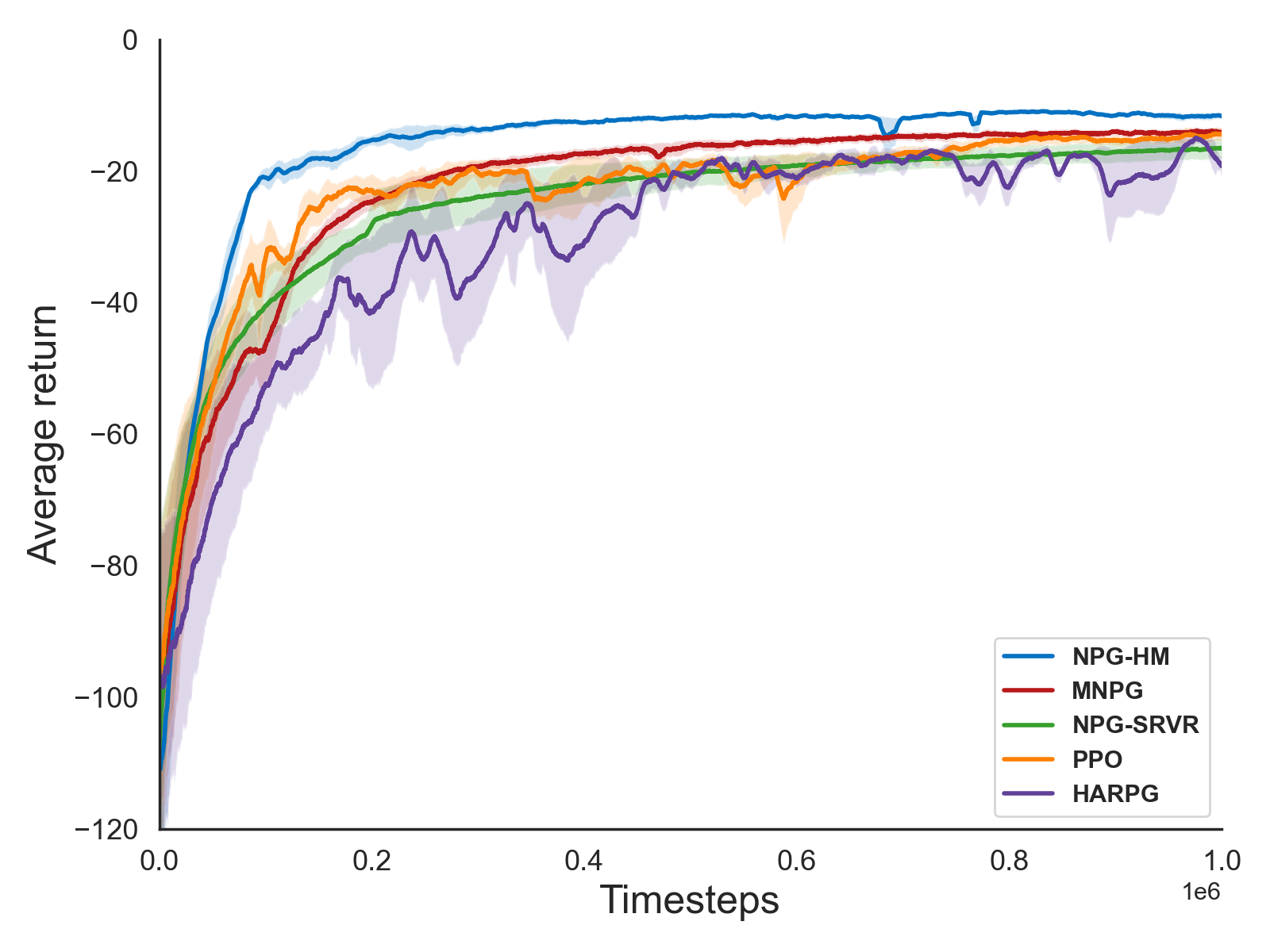
(a) Reacher

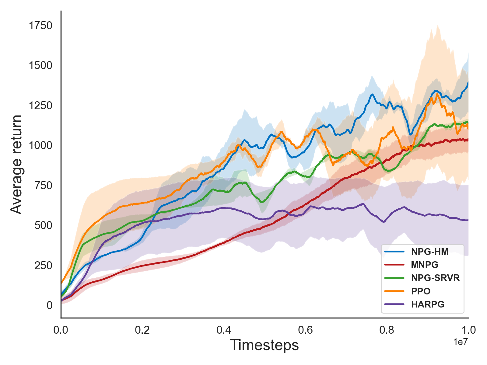
(b) Hopper

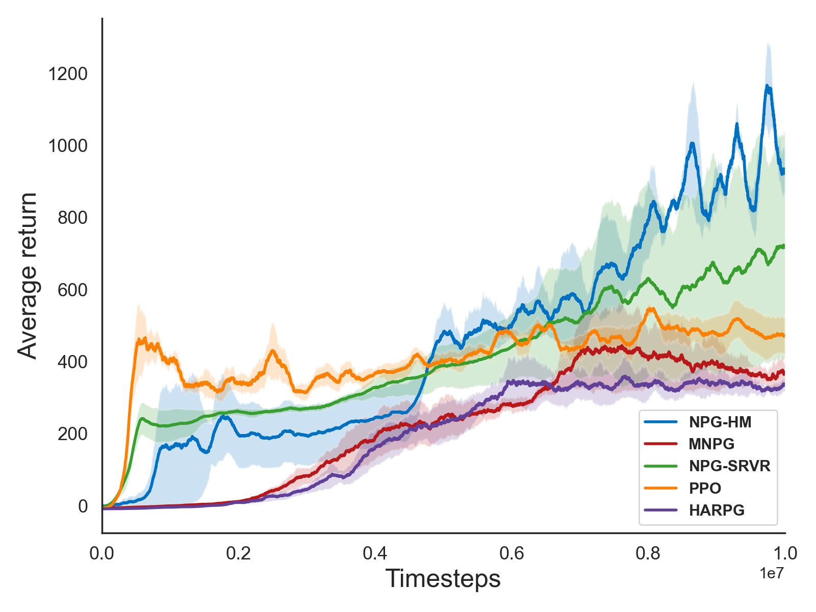
(c) Walker2d

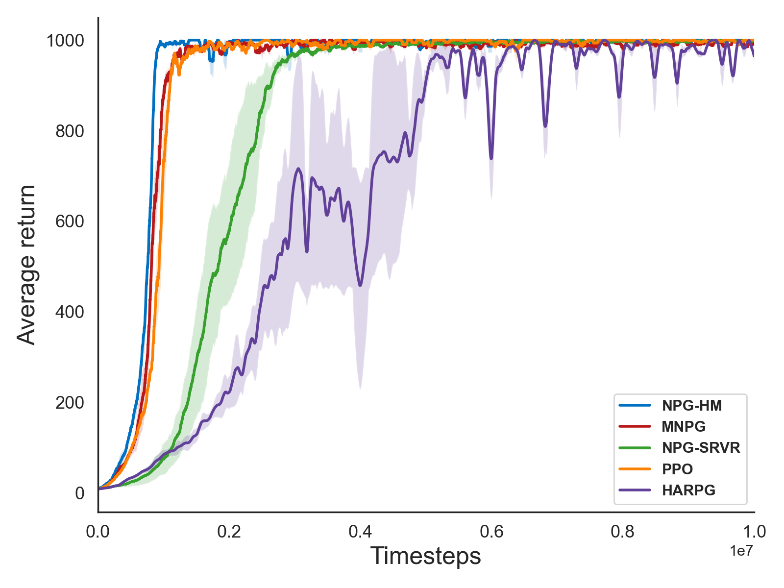
(d) Pendulum

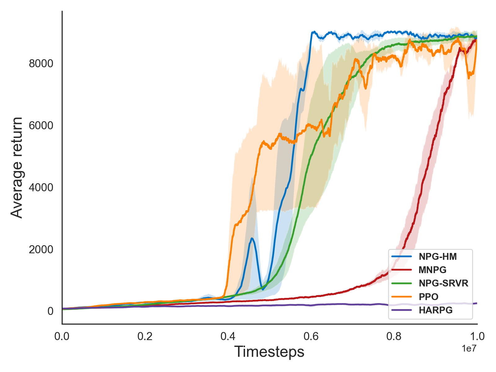
(e) DoublePendulum

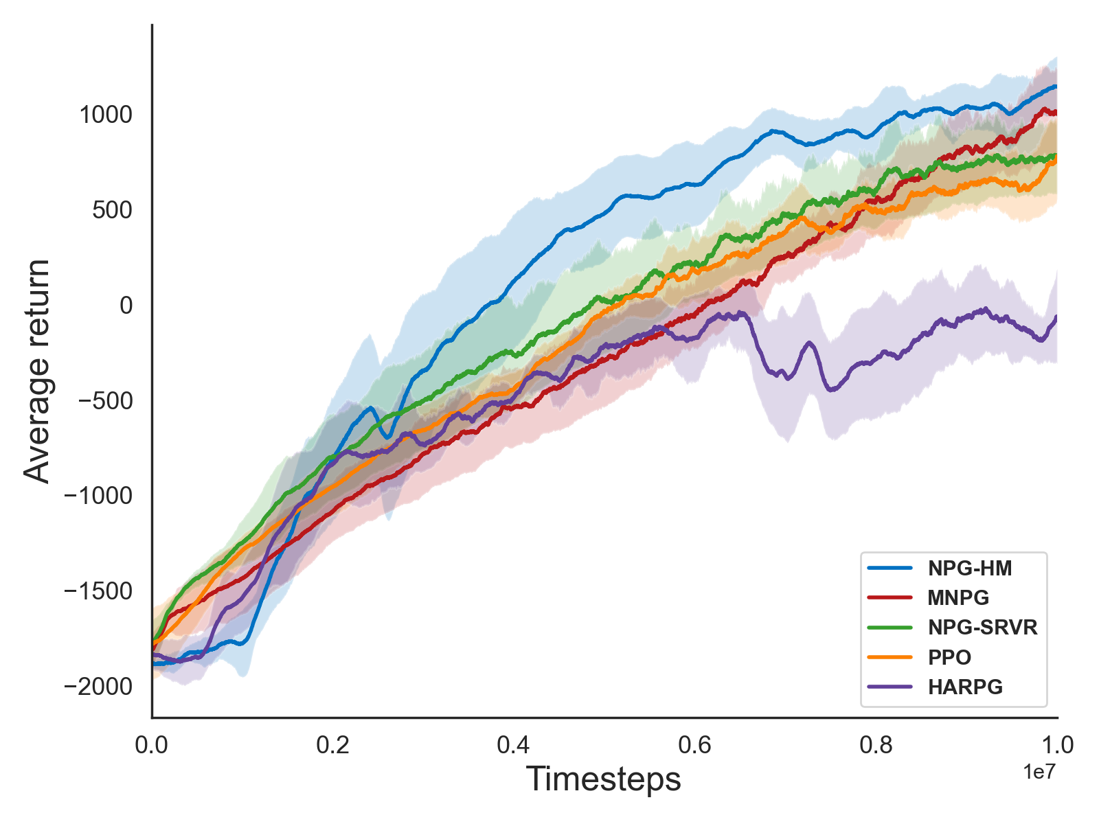
(f) HalfCheetah

Figure 1: Empirical comparison of NPG-HM and other policy gradient methods on six environments.

6 Conclusions

In this paper, we have proposed a new algorithm termed NPG-HM for RL, which is a sample-based NPG method with Hessian-aided moment variance reduction. The ${\cal O}(\varepsilon^{-2})$ sample complexity for NPG-HM to achieve the global last-iterate convergence has been established, which matches the best known result under the general Fisher-non-degenerate policy. Numerical results have been conducted to demonstrate the superiority of NPG-HM compared to other state-of-the-art policy gradient methods. There are several directions for future research. Firstly, it is possible to extend NPG-HM to the multi-agent setting and investigate the convergence properties. Furthermore, regularization-based NPG methods have been widely investigated in recent studies. Therefore a possible future work is to study NPG-HM for the regularized RL problem. Lastly, it is also interesting to design more efficient subroutines to compute the update direction in NPG-HM to improve the computational efficiency.

7 Proofs of Technical Lemmas

7.1 Proof of Lemma 4.5

We will apply Lemma 4.4 to prove this lemma. Recall the definitions of $\bm{w}_{o}(\bm{u},\bm{\theta})$ and $\widehat{\bm{w}}(\bm{u},\bm{\theta})$ in the statement of the lemma. Let $\bm{w}_{o}=\bm{w}_{o}(\bm{u},\bm{\theta}),\widehat{\bm{w}}=\widehat{\bm{w}}(\bm{u},\bm{\theta})$, $\bm{x}_{k}=\nabla\log\pi_{\bm{\theta}}(a_{k}|s_{k}),\bm{z}_{k}=\bm{u}$ and $\xi_{k}=\bm{u}-\left\langle\widehat{\bm{w}},\bm{x}_{k}\right\rangle\bm{x}_{k}$ for simplicity. A direct computation yields that

$$\left\|\bm{x}_{k}\right\|_{{\footnotesize{2}}}^{2} \leq M_{g},$$

$$\left(\widehat{\bm{w}}^{\mathsf{T}}\bm{x}_{k}\right)^{2} \leq\left\|\bm{x}_{k}\right\|_{{\footnotesize{2}}}^{2}\cdot\left\|\widehat{\bm{w}}\right\|_{{\footnotesize{2}}}^{2}\leq M_{g}\left\|\bm{F}^{-1}(\bm{\theta})\bm{u}\right\|_{{\footnotesize{2}}}^{2}\leq\frac{M_{g}}{\mu_{F}^{2}}\left\|\bm{u}\right\|_{{\footnotesize{2}}}^{2},$$

$$\mathbb{E}_{(s,a)}\left\{\xi_{k}\xi_{k}^{\mathsf{T}}\rule{0.0pt}{8.53581pt}\right\} \preccurlyeq\frac{M_{g}}{\mu_{F}^{2}}\left\|\bm{u}\right\|_{{\footnotesize{2}}}^{2}\mathbb{E}_{(s,a)}\left\{\bm{x}_{k}\bm{x}_{k}^{\mathsf{T}}\rule{0.0pt}{8.53581pt}\right\}+\frac{\left\|\bm{u}\right\|_{{\footnotesize{2}}}^{2}}{\mu_{F}}\mathbb{E}_{(s,a)}\left\{\bm{x}_{k}\bm{x}_{k}^{\mathsf{T}}\rule{0.0pt}{8.53581pt}\right\}$$

$$\preccurlyeq\frac{2M_{g}}{\mu_{F}^{2}}\left\|\bm{u}\right\|_{{\footnotesize{2}}}^{2}\mathbb{E}_{(s,a)}\left\{\bm{x}_{k}\bm{x}_{k}^{\mathsf{T}}\rule{0.0pt}{8.53581pt}\right\}:=\sigma^{2}\mathbb{E}_{(s,a)}\left\{\bm{x}_{k}\bm{x}_{k}^{\mathsf{T}}\rule{0.0pt}{8.53581pt}\right\},$$

$$\mathbb{E}_{(s,a)}\left\{\left\|\bm{x}_{k}\right\|_{{\footnotesize{2}}}^{2}\bm{x}_{k}\bm{x}_{k}^{\mathsf{T}}\rule{0.0pt}{8.53581pt}\right\} \preccurlyeq M_{g}\mathbb{E}_{(s,a)}\left\{\bm{x}_{k}\bm{x}_{k}^{\mathsf{T}}\rule{0.0pt}{8.53581pt}\right\}:=R^{2}\mathbb{E}_{(s,a)}\left\{\bm{x}_{k}\bm{x}_{k}^{\mathsf{T}}\rule{0.0pt}{8.53581pt}\right\},$$

where $\sigma^{2}=\frac{2M_{g}}{\mu_{F}^{2}}\left\|\bm{u}\right\|_{{\footnotesize{2}}}^{2}$ and $R^{2}=M_{g}$. Thus the application of Lemma 4.4 yields that

$$\mathbb{E}\left\{\left\|\bm{w}_{o}-\widehat{\bm{w}}\right\|_{{\footnotesize{2}}}^{2}\rule{0.0pt}{8.53581pt}\right\} \leq\frac{2}{\mu_{F}}\mathbb{E}\left\{f(\bm{w}_{o})-f(\widehat{\bm{w}})\rule{0.0pt}{8.53581pt}\right\}$$

$$\leq\frac{2}{\mu_{F}}\cdot\frac{2}{K}\left(\sigma\sqrt{d}+R\left\|\bm{w}^{0}-\widehat{\bm{w}}\right\|_{{\footnotesize{2}}}\right)^{2}$$

$$=\frac{2}{\mu_{F}}\cdot\frac{2}{K}\left(\sqrt{\frac{2M_{g}d}{\mu_{F}^{2}}}\left\|\bm{u}\right\|_{{\footnotesize{2}}}+\sqrt{M_{g}}\left\|\widehat{\bm{w}}\right\|_{{\footnotesize{2}}}\right)^{2}$$

$$=\frac{2}{\mu_{F}}\cdot\frac{2}{K}\left(\sqrt{\frac{2M_{g}d}{\mu_{F}^{2}}}\left\|\bm{u}\right\|_{{\footnotesize{2}}}+\sqrt{M_{g}}\left\|\bm{F}^{-1}(\bm{\theta})\bm{u}\right\|_{{\footnotesize{2}}}\right)^{2}$$

$$\leq\frac{2}{\mu_{F}}\cdot\frac{2}{K}\left(\sqrt{\frac{2M_{g}d}{\mu_{F}^{2}}}\left\|\bm{u}\right\|_{{\footnotesize{2}}}+\frac{\sqrt{M_{g}}}{\mu_{F}}\left\|\bm{u}\right\|_{{\footnotesize{2}}}\right)^{2}$$

$$=\frac{4M_{g}(\sqrt{2d}+1)^{2}}{K\mu_{F}^{3}}\left\|\bm{u}\right\|_{{\footnotesize{2}}}^{2},$$

which completes the proof.

7.2 Proof of Lemma 4.6

By Assumption 3.2, we know that

$$\varepsilon_{\operatorname{bias}} \geq\mathbb{E}_{(s,a)\sim\tilde{d}_{\rho,\pi^{\ast}}}\left\{\left(A^{\pi_{\bm{\theta}}}(s,a)-(1-\gamma){\bm{w}^{\ast}_{\bm{\theta}}}^{\mathsf{T}}\nabla\log\pi_{\bm{\theta}}(a|s)\right)^{2}\rule{0.0pt}{8.53581pt}\right\}$$

$$\geq\left(\mathbb{E}_{(s,a)\sim\tilde{d}_{\rho,\pi^{\ast}}}\left\{A^{\pi_{\bm{\theta}}}(s,a)\rule{0.0pt}{8.53581pt}\right\}-(1-\gamma)\mathbb{E}_{(s,a)\sim\tilde{d}_{\rho,\pi^{\ast}}}\left\{{\bm{w}^{\ast}_{\bm{\theta}}}^{\mathsf{T}}\nabla\log\pi_{\bm{\theta}}(a|s)\rule{0.0pt}{8.53581pt}\right\}\right)^{2}$$

$$=(1-\gamma)^{2}\left(J_{\rho}^{\ast}-J_{\rho}(\bm{\theta})-\mathbb{E}_{(s,a)\sim\tilde{d}_{\rho,\pi^{\ast}}}\left\{{\bm{w}^{\ast}_{\bm{\theta}}}^{\mathsf{T}}\nabla\log\pi_{\bm{\theta}}(a|s)\rule{0.0pt}{8.53581pt}\right\}\right)^{2},$$

where the second line is due to Jensen’s inequality and the last line follows from the performance difference lemma of [18], i.e.,

$$J_{\rho}^{\ast}-J_{\rho}(\bm{\theta})=\frac{1}{1-\gamma}\mathbb{E}_{(s,a)\sim\tilde{d}_{\rho,\pi^{\ast}}}\left\{A^{\pi_{\bm{\theta}}}(s,a)\rule{0.0pt}{8.53581pt}\right\}.$$

After rearrangement one has

$$\frac{\sqrt{\varepsilon_{\operatorname{bias}}}}{1-\gamma} \geq J_{\rho}^{\ast}-J_{\rho}(\bm{\theta})-\mathbb{E}_{(s,a)\sim\tilde{d}_{\rho,\pi^{\ast}}}\left\{{\bm{w}^{\ast}_{\bm{\theta}}}^{\mathsf{T}}\nabla\log\pi_{\bm{\theta}}(a|s)\rule{0.0pt}{8.53581pt}\right\}$$

$$\geq J_{\rho}^{\ast}-J_{\rho}(\bm{\theta})-\sqrt{M_{g}}\left\|\bm{w}^{\ast}_{\bm{\theta}}\right\|_{{\footnotesize{2}}},$$

where the last line is due to Assumption 3.1. It follows that

$$M_{g}\left\|\bm{w}^{\ast}_{\bm{\theta}}\right\|_{{\footnotesize{2}}}^{2}+\frac{\varepsilon_{\operatorname{bias}}}{(1-\gamma)^{2}} \geq\frac{1}{2}\left(\sqrt{M_{g}}\left\|\bm{w}^{\ast}_{\bm{\theta}}\right\|_{{\footnotesize{2}}}+\frac{\sqrt{\varepsilon_{\operatorname{bias}}}}{1-\gamma}\right)^{2}$$

$$\geq\frac{1}{2}(J_{\rho}^{\ast}-J_{\rho}(\bm{\theta}))^{2},$$

which completes the proof.

7.3 Proof of Lemma 4.7

Recall that $\bm{w}_{t}$ is the output of Algorithm 2, $\bm{w}_{t}^{\ast}$ is a minimizer of (2.10), and $\widehat{\bm{w}}_{t}$ is a minimizer of (3.1). Since $J_{\rho}(\cdot)$ is $L$-smooth (Lemma 4.1), we have

$$J_{\rho}(\bm{\theta}_{t+1}) \geq J_{\rho}(\bm{\theta}_{t})+\left\langle\nabla J_{\rho}(\bm{\theta}_{t}),\bm{\theta}_{t+1}-\bm{\theta}_{t}\right\rangle-\frac{L}{2}\left\|\bm{\theta}_{t+1}-\bm{\theta}_{t}\right\|_{{\footnotesize{2}}}^{2}$$

$$\stackrel{{\scriptstyle(a)}}{{=}}J_{\rho}(\bm{\theta}_{t})+\alpha_{t}\left\langle\nabla J_{\rho}(\bm{\theta}_{t}),\bm{w}_{t}\right\rangle-\frac{L\alpha_{t}^{2}}{2}\left\|\bm{w}_{t}\right\|_{{\footnotesize{2}}}^{2}$$

$$\stackrel{{\scriptstyle(b)}}{{=}}J_{\rho}(\bm{\theta}_{t})+\alpha_{t}\left\langle\bm{F}(\bm{\theta}_{t})\bm{w}_{t}^{\ast},\bm{w}_{t}\right\rangle-\frac{L\alpha_{t}^{2}}{2}\left\|\bm{w}_{t}\right\|_{{\footnotesize{2}}}^{2}$$

$$\stackrel{{\scriptstyle(c)}}{{=}}J_{\rho}(\bm{\theta}_{t})+\frac{\alpha_{t}}{2}\left\langle\bm{F}(\bm{\theta}_{t})\bm{w}_{t}^{\ast},\bm{w}_{t}^{\ast}\right\rangle+\frac{\alpha_{t}}{2}\left\langle\bm{F}(\bm{\theta}_{t})\bm{w}_{t},\bm{w}_{t}\right\rangle$$

$$\quad-\frac{\alpha_{t}}{2}\left\langle\bm{F}(\bm{\theta}_{t})(\bm{w}_{t}^{\ast}-\bm{w}_{t}),\bm{w}_{t}^{\ast}-\bm{w}_{t}\right\rangle-\frac{L\alpha_{t}^{2}}{2}\left\|\bm{w}_{t}\right\|_{{\footnotesize{2}}}^{2}$$

$$\geq J_{\rho}(\bm{\theta}_{t})+\frac{\alpha_{t}\mu_{F}}{2}\left\|\bm{w}_{t}^{\ast}\right\|_{{\footnotesize{2}}}^{2}+\frac{\alpha_{t}\mu_{F}}{2}\left\|\bm{w}_{t}\right\|_{{\footnotesize{2}}}^{2}-\frac{\alpha_{t}M_{g}}{2}\left\|\bm{w}_{t}^{\ast}-\bm{w}_{t}\right\|_{{\footnotesize{2}}}^{2}-\frac{L\alpha_{t}^{2}}{2}\left\|\bm{w}_{t}\right\|_{{\footnotesize{2}}}^{2}$$

$$=J_{\rho}(\bm{\theta}_{t})+\frac{\alpha_{t}\mu_{F}}{2}\left\|\bm{w}_{t}^{\ast}\right\|_{{\footnotesize{2}}}^{2}+\left(\frac{\alpha_{t}\mu_{F}}{2}-\frac{L\alpha_{t}^{2}}{2}\right)\left\|\bm{w}_{t}\right\|_{{\footnotesize{2}}}^{2}-\frac{\alpha_{t}M_{g}}{2}\left\|\bm{w}_{t}^{\ast}-\bm{w}_{t}\right\|_{{\footnotesize{2}}}^{2}$$

$$\geq J_{\rho}(\bm{\theta}_{t})+\frac{\alpha_{t}\mu_{F}}{2}\left\|\bm{w}_{t}^{\ast}\right\|_{{\footnotesize{2}}}^{2}+\left(\frac{\alpha_{t}\mu_{F}}{2}-\frac{L\alpha_{t}^{2}}{2}\right)\left\|\bm{w}_{t}\right\|_{{\footnotesize{2}}}^{2}$$

$$\quad-\alpha_{t}M_{g}\left\|\bm{w}_{t}^{\ast}-\widehat{\bm{w}}_{t}\right\|_{{\footnotesize{2}}}^{2}-\alpha_{t}M_{g}\left\|\bm{w}_{t}-\widehat{\bm{w}}_{t}\right\|_{{\footnotesize{2}}}^{2}$$

$$=J_{\rho}(\bm{\theta}_{t})+\frac{\alpha_{t}\mu_{F}}{2}\left\|\bm{w}_{t}^{\ast}\right\|_{{\footnotesize{2}}}^{2}+\left(\frac{\alpha_{t}\mu_{F}}{2}-\frac{L\alpha_{t}^{2}}{2}\right)\left\|\bm{w}_{t}\right\|_{{\footnotesize{2}}}^{2}$$

$$\quad-\alpha_{t}M_{g}\left\|\bm{F}^{-1}(\bm{\theta}_{t})\left(\nabla J_{\rho}(\bm{\theta})-\bm{u}_{t}\right)\right\|_{{\footnotesize{2}}}^{2}-\alpha_{t}M_{g}\left\|\bm{w}_{t}-\widehat{\bm{w}}_{t}\right\|_{{\footnotesize{2}}}^{2}$$

$$\geq J_{\rho}(\bm{\theta}_{t})+\frac{\alpha_{t}\mu_{F}}{2}\left\|\bm{w}_{t}^{\ast}\right\|_{{\footnotesize{2}}}^{2}+\left(\frac{\alpha_{t}\mu_{F}}{2}-\frac{L\alpha_{t}^{2}}{2}\right)\left\|\bm{w}_{t}\right\|_{{\footnotesize{2}}}^{2}$$

$$\quad-\frac{\alpha_{t}M_{g}}{\mu_{F}^{2}}\left\|\nabla J_{\rho}(\bm{\theta})-\bm{u}_{t}\right\|_{{\footnotesize{2}}}^{2}-\alpha_{t}M_{g}\left\|\bm{w}_{t}-\widehat{\bm{w}}_{t}\right\|_{{\footnotesize{2}}}^{2}$$

$$\geq J_{\rho}(\bm{\theta}_{t})+\frac{\alpha_{t}\mu_{F}}{2}\left\|\bm{w}_{t}^{\ast}\right\|_{{\footnotesize{2}}}^{2}+\left(\frac{\alpha_{t}\mu_{F}}{2}-\frac{L\alpha_{t}^{2}}{2}\right)\left\|\bm{w}_{t}\right\|_{{\footnotesize{2}}}^{2}$$

$$\quad-\frac{2\alpha_{t}M_{g}}{\mu_{F}^{2}}\left\|\nabla J_{\rho}(\bm{\theta})-\nabla J_{\rho}^{H}(\bm{\theta}_{t})\right\|_{{\footnotesize{2}}}^{2}-\frac{2\alpha_{t}M_{g}}{\mu_{F}^{2}}\left\|\nabla J_{\rho}^{H}(\bm{\theta}_{t})-\bm{u}_{t}\right\|_{{\footnotesize{2}}}^{2}-\alpha_{t}M_{g}\left\|\bm{w}_{t}-\widehat{\bm{w}}_{t}\right\|_{{\footnotesize{2}}}^{2}$$

$$\stackrel{{\scriptstyle(d)}}{{\geq}}J_{\rho}(\bm{\theta}_{t})+\frac{\alpha_{t}\mu_{F}}{2}\left\|\bm{w}_{t}^{\ast}\right\|_{{\footnotesize{2}}}^{2}+\left(\frac{\alpha_{t}\mu_{F}}{2}-\frac{L\alpha_{t}^{2}}{2}\right)\left\|\bm{w}_{t}\right\|_{{\footnotesize{2}}}^{2}$$

$$\quad-\frac{2\alpha_{t}M_{g}}{\mu_{F}^{2}}G_{g}^{2}\gamma^{2H}-\frac{2\alpha_{t}M_{g}}{\mu_{F}^{2}}\left\|\nabla J_{\rho}^{H}(\bm{\theta}_{t})-\bm{u}_{t}\right\|_{{\footnotesize{2}}}^{2}-\alpha_{t}M_{g}\left\|\bm{w}_{t}-\widehat{\bm{w}}_{t}\right\|_{{\footnotesize{2}}}^{2}$$

$$\geq J_{\rho}(\bm{\theta}_{t})+\frac{\alpha_{t}\mu_{F}}{2}\left\|\bm{w}_{t}^{\ast}\right\|_{{\footnotesize{2}}}^{2}+\frac{\alpha_{t}\mu_{F}}{4}\left\|\bm{w}_{t}\right\|_{{\footnotesize{2}}}^{2}$$

$$\quad-\frac{2\alpha_{t}M_{g}}{\mu_{F}^{2}}G_{g}^{2}\gamma^{2H}-\frac{2\alpha_{t}M_{g}}{\mu_{F}^{2}}\left\|\nabla J_{\rho}^{H}(\bm{\theta}_{t})-\bm{u}_{t}\right\|_{{\footnotesize{2}}}^{2}-\alpha_{t}M_{g}\left\|\bm{w}_{t}-\widehat{\bm{w}}_{t}\right\|_{{\footnotesize{2}}}^{2},$$

where step (a) is due to the update rule $\bm{\theta}_{t+1}=\bm{\theta}_{t}+\alpha_{t}\bm{w}_{t}$, step (b) is due to the definition $\bm{w}_{t}^{\ast}=\bm{F}^{-1}(\bm{\theta}_{t})\nabla J_{\rho}(\bm{\theta}_{t})$, step (c) follows from $\bm{a}^{\mathsf{T}}\bm{M}\bm{b}=\frac{1}{2}\left(\bm{a}^{\mathsf{T}}\bm{M}\bm{a}+\bm{b}^{\mathsf{T}}\bm{M}\bm{b}-(\bm{a}-\bm{b})^{\mathsf{T}}\bm{M}(\bm{a}-\bm{b})\right)$ for any $\bm{a},\bm{b}$ and any symmetric matrix $\bm{M}$, step (d) holds by Lemma 4.3, and the last line is due to $\alpha_{t}\leq\frac{\mu_{F}}{2L}$.

7.4 Proof of Lemma 4.8

By Lemma 4.7, one has

$$\mathbb{E}\left\{J_{\rho}(\bm{\theta}_{t+1})\rule{0.0pt}{8.53581pt}\right\} \geq\mathbb{E}\left\{J_{\rho}(\bm{\theta}_{t})\rule{0.0pt}{8.53581pt}\right\}+\frac{\alpha_{t}\mu_{F}}{2}\mathbb{E}\left\{\left\|\bm{w}_{t}^{\ast}\right\|_{{\footnotesize{2}}}^{2}\rule{0.0pt}{8.53581pt}\right\}+\frac{\alpha_{t}\mu_{F}}{4}\mathbb{E}\left\{\left\|\bm{w}_{t}\right\|_{{\footnotesize{2}}}^{2}\rule{0.0pt}{8.53581pt}\right\}-\frac{2\alpha_{t}M_{g}}{\mu_{F}^{2}}G_{g}^{2}\gamma^{2H}$$

$$\quad-\frac{2\alpha_{t}M_{g}}{\mu_{F}^{2}}\mathbb{E}\left\{\left\|\nabla J_{\rho}^{H}(\bm{\theta}_{t})-\bm{u}_{t}\right\|_{{\footnotesize{2}}}^{2}\rule{0.0pt}{8.53581pt}\right\}-\alpha_{t}M_{g}\mathbb{E}\left\{\left\|\bm{w}_{t}-\widehat{\bm{w}}_{t}\right\|_{{\footnotesize{2}}}^{2}\rule{0.0pt}{8.53581pt}\right\}$$

$$=\mathbb{E}\left\{J_{\rho}(\bm{\theta}_{t})\rule{0.0pt}{8.53581pt}\right\}+\frac{\alpha_{t}\mu_{F}}{2}\mathbb{E}\left\{\left\|\bm{w}_{t}^{\ast}\right\|_{{\footnotesize{2}}}^{2}\rule{0.0pt}{8.53581pt}\right\}+\frac{\mu_{F}}{4\alpha_{t}}R_{t}-\frac{2\alpha_{t}M_{g}}{\mu_{F}^{2}}G_{g}^{2}\gamma^{2H}$$

$$\qquad-\frac{2\alpha_{t}M_{g}}{\mu_{F}^{2}}V_{t}-\alpha_{t}M_{g}\mathbb{E}\left\{\left\|\bm{w}_{t}-\widehat{\bm{w}}_{t}\right\|_{{\footnotesize{2}}}^{2}\rule{0.0pt}{8.53581pt}\right\}.$$ (7.1)

Notice that $\bm{w}_{t}$ is the output of Algorithm 2 and $\widehat{\bm{w}}_{t}$ is the minimizer of (3.1) given $(\bm{u}_{t},\bm{\theta}_{t})$. Then conditioned on $\bm{u}_{t}$ and $\bm{\theta}_{t}$, applying Lemma 4.5 with $(\bm{u}=\bm{u}_{t},\bm{\theta}=\bm{\theta}_{t})$ yields that

$$\mathbb{E}_{(s_{k},a_{k})_{k=0,\cdots,K-1}}\left\{\left\|\bm{w}_{t}-\widehat{\bm{w}}_{t}\right\|_{{\footnotesize{2}}}^{2}\rule{0.0pt}{8.53581pt}\right\} =\mathbb{E}_{(s_{k},a_{k})_{k=0,\cdots,K-1}}\left\{\left\|\bm{w}_{o}(\bm{u}_{t},\bm{\theta}_{t})-\widehat{\bm{w}}(\bm{u}_{t},\bm{\theta}_{t})\right\|_{{\footnotesize{2}}}^{2}\rule{0.0pt}{8.53581pt}\right\}$$

$$\leq\frac{4M_{g}(\sqrt{2d}+1)^{2}}{K\mu_{F}^{3}}\left\|\bm{u}_{t}\right\|_{{\footnotesize{2}}}^{2}.$$

Taking expectation on both sides yields that

$$\mathbb{E}\left\{\left\|\bm{w}_{t}-\widehat{\bm{w}}_{t}\right\|_{{\footnotesize{2}}}^{2}\rule{0.0pt}{8.53581pt}\right\}$$

$$\leq\frac{4M_{g}(\sqrt{2d}+1)^{2}}{K\mu_{F}^{3}}\mathbb{E}\left\{\left\|\bm{u}_{t}\right\|_{{\footnotesize{2}}}^{2}\rule{0.0pt}{8.53581pt}\right\}$$

$$\leq\frac{12M_{g}(\sqrt{2d}+1)^{2}}{K\mu_{F}^{3}}\left(\mathbb{E}\left\{\left\|\bm{u}_{t}-\nabla J_{\rho}^{H}(\bm{\theta}_{t})\right\|_{{\footnotesize{2}}}^{2}\rule{0.0pt}{8.53581pt}\right\}+\mathbb{E}\left\{\left\|\nabla J_{\rho}^{H}(\bm{\theta}_{t})-\nabla J_{\rho}(\bm{\theta}_{t})\right\|_{{\footnotesize{2}}}^{2}\rule{0.0pt}{8.53581pt}\right\}+\mathbb{E}\left\{\left\|\nabla J_{\rho}(\bm{\theta}_{t})\right\|_{{\footnotesize{2}}}^{2}\rule{0.0pt}{8.53581pt}\right\}\right)$$

$$=\frac{12M_{g}(\sqrt{2d}+1)^{2}}{K\mu_{F}^{3}}\left(\mathbb{E}\left\{\left\|\bm{u}_{t}-\nabla J_{\rho}^{H}(\bm{\theta}_{t})\right\|_{{\footnotesize{2}}}^{2}\rule{0.0pt}{8.53581pt}\right\}+\mathbb{E}\left\{\left\|\nabla J_{\rho}^{H}(\bm{\theta}_{t})-\nabla J_{\rho}(\bm{\theta}_{t})\right\|_{{\footnotesize{2}}}^{2}\rule{0.0pt}{8.53581pt}\right\}+\mathbb{E}\left\{\left\|\bm{F}(\bm{\theta}_{t})\bm{w}_{t}^{\ast}\right\|_{{\footnotesize{2}}}^{2}\rule{0.0pt}{8.53581pt}\right\}\right)$$

$$\leq\frac{12M_{g}(\sqrt{2d}+1)^{2}}{K\mu_{F}^{3}}\left(\mathbb{E}\left\{\left\|\bm{u}_{t}-\nabla J_{\rho}^{H}(\bm{\theta}_{t})\right\|_{{\footnotesize{2}}}^{2}\rule{0.0pt}{8.53581pt}\right\}+G_{g}^{2}\gamma^{2H}+M_{g}^{2}\mathbb{E}\left\{\left\|\bm{w}_{t}^{\ast}\right\|_{{\footnotesize{2}}}^{2}\rule{0.0pt}{8.53581pt}\right\}\right)$$

$$=\frac{12M_{g}(\sqrt{2d}+1)^{2}}{K\mu_{F}^{3}}\left(V_{t}+M_{g}^{2}\mathbb{E}\left\{\left\|\bm{w}_{t}^{\ast}\right\|_{{\footnotesize{2}}}^{2}\rule{0.0pt}{8.53581pt}\right\}+G_{g}^{2}\gamma^{2H}\right).$$ (7.2)

After plugging (7.2) into (7.1), one has

$$\mathbb{E}\left\{J_{\rho}(\bm{\theta}_{t+1})\rule{0.0pt}{8.53581pt}\right\} \geq\mathbb{E}\left\{J_{\rho}(\bm{\theta}_{t})\rule{0.0pt}{8.53581pt}\right\}+\frac{\alpha_{t}\mu_{F}}{2}\mathbb{E}\left\{\left\|\bm{w}_{t}^{\ast}\right\|_{{\footnotesize{2}}}^{2}\rule{0.0pt}{8.53581pt}\right\}+\frac{\mu_{F}}{4\alpha_{t}}R_{t}-\frac{2\alpha_{t}M_{g}}{\mu_{F}^{2}}G_{g}^{2}\gamma^{2H}-\frac{2\alpha_{t}M_{g}}{\mu_{F}^{2}}V_{t}$$

$$\quad-\alpha_{t}M_{g}\left(\frac{12M_{g}(\sqrt{2d}+1)^{2}}{K\mu_{F}^{3}}V_{t}+\frac{12M_{g}^{3}(\sqrt{2d}+1)^{2}}{K\mu_{F}^{3}}\mathbb{E}\left\{\left\|\bm{w}_{t}^{\ast}\right\|_{{\footnotesize{2}}}^{2}\rule{0.0pt}{8.53581pt}\right\}+\frac{12M_{g}(\sqrt{2d}+1)^{2}}{K\mu_{F}^{3}}G_{g}^{2}\gamma^{2H}\right)$$

$$=\mathbb{E}\left\{J_{\rho}(\bm{\theta}_{t})\rule{0.0pt}{8.53581pt}\right\}+\left(\frac{\alpha_{t}\mu_{F}}{2}-\frac{12\alpha_{t}M_{g}^{4}(\sqrt{2d}+1)^{2}}{K\mu_{F}^{3}}\right)\mathbb{E}\left\{\left\|\bm{w}_{t}^{\ast}\right\|_{{\footnotesize{2}}}^{2}\rule{0.0pt}{8.53581pt}\right\}+\frac{\mu_{F}}{4\alpha_{t}}R_{t}$$

$$\quad-\left(\frac{2\alpha_{t}M_{g}}{\mu_{F}^{2}}+\frac{12\alpha_{t}M_{g}^{2}(\sqrt{2d}+1)^{2}}{K\mu_{F}^{3}}\right)G_{g}^{2}\gamma^{2H}-\left(\frac{2\alpha_{t}M_{g}}{\mu_{F}^{2}}+\frac{12\alpha_{t}M_{g}^{2}(\sqrt{2d}+1)^{2}}{K\mu_{F}^{3}}\right)V_{t}$$

$$=\mathbb{E}\left\{J_{\rho}(\bm{\theta}_{t})\rule{0.0pt}{8.53581pt}\right\}+\frac{\alpha_{t}\mu_{F}}{2}\left(1-\frac{24\kappa^{4}(\sqrt{2d}+1)^{2}}{K}\right)\mathbb{E}\left\{\left\|\bm{w}_{t}^{\ast}\right\|_{{\footnotesize{2}}}^{2}\rule{0.0pt}{8.53581pt}\right\}+\frac{\mu_{F}}{4\alpha_{t}}R_{t}$$

$$\quad-\frac{2\alpha_{t}M_{g}}{\mu_{F}^{2}}\left(1+\frac{6\kappa(\sqrt{2d}+1)^{2}}{K}\right)G_{g}^{2}\gamma^{2H}-\frac{2\alpha_{t}M_{g}}{\mu_{F}^{2}}\left(1+\frac{6\kappa(\sqrt{2d}+1)^{2}}{K}\right)V_{t}$$

$$\geq\mathbb{E}\left\{J_{\rho}(\bm{\theta}_{t})\rule{0.0pt}{8.53581pt}\right\}+\frac{c_{1}\alpha_{t}\mu_{F}}{2}\mathbb{E}\left\{\left\|\bm{w}_{t}^{\ast}\right\|_{{\footnotesize{2}}}^{2}\rule{0.0pt}{8.53581pt}\right\}+\frac{\mu_{F}}{4\alpha_{t}}R_{t}-\frac{4\alpha_{t}M_{g}}{\mu_{F}^{2}}G_{g}^{2}\gamma^{2H}-\frac{4\alpha_{t}M_{g}}{\mu_{F}^{2}}V_{t},$$

where the last line is due to $K\geq 48\kappa^{4}(\sqrt{2d}+1)^{2}$, i.e.

$$c_{1}:=1-\frac{24\kappa^{4}(\sqrt{2d}+1)^{2}}{K}\geq\frac{1}{2}\text{ and }c_{2}:=1+\frac{6\kappa(\sqrt{2d}+1)^{2}}{K}\leq 2.$$

Furthermore, the application of Lemma 4.6 yields that

$$\mathbb{E}\left\{J_{\rho}(\bm{\theta}_{t+1})\rule{0.0pt}{8.53581pt}\right\} \geq\mathbb{E}\left\{J_{\rho}(\bm{\theta}_{t})\rule{0.0pt}{8.53581pt}\right\}+\frac{c_{1}\alpha_{t}\mu_{F}}{2}\left(\frac{1}{2M_{g}}\mathbb{E}\left\{(J_{\rho}^{\ast}-J_{\rho}(\bm{\theta}_{t}))^{2}\rule{0.0pt}{8.53581pt}\right\}-\frac{\varepsilon_{\operatorname{bias}}}{M_{g}(1-\gamma)^{2}}\right)$$

$$\qquad+\frac{\mu_{F}}{4\alpha_{t}}R_{t}-\frac{4\alpha_{t}M_{g}}{\mu_{F}^{2}}G_{g}^{2}\gamma^{2H}-\frac{4\alpha_{t}M_{g}}{\mu_{F}^{2}}V_{t}$$

$$=\mathbb{E}\left\{J_{\rho}(\bm{\theta}_{t})\rule{0.0pt}{8.53581pt}\right\}+\frac{c_{1}\alpha_{t}}{4\kappa}\mathbb{E}\left\{(J_{\rho}^{\ast}-J_{\rho}(\bm{\theta}_{t}))^{2}\rule{0.0pt}{8.53581pt}\right\}-\frac{c_{1}\alpha_{t}\varepsilon_{\operatorname{bias}}}{2\kappa(1-\gamma)^{2}}+\frac{\mu_{F}}{4\alpha_{t}}R_{t}-\frac{4\alpha_{t}M_{g}}{\mu_{F}^{2}}G_{g}^{2}\gamma^{2H}-\frac{4\alpha_{t}M_{g}}{\mu_{F}^{2}}V_{t}$$

$$\geq\mathbb{E}\left\{J_{\rho}(\bm{\theta}_{t})\rule{0.0pt}{8.53581pt}\right\}+\frac{c_{1}\alpha_{t}}{4\kappa}\left(\mathbb{E}\left\{J_{\rho}^{\ast}-J_{\rho}(\bm{\theta}_{t})\rule{0.0pt}{8.53581pt}\right\}\right)^{2}-\frac{\alpha_{t}\varepsilon_{\operatorname{bias}}}{2\kappa(1-\gamma)^{2}}+\frac{\mu_{F}}{4\alpha_{t}}R_{t}-\frac{4\alpha_{t}M_{g}}{\mu_{F}^{2}}G_{g}^{2}\gamma^{2H}-\frac{4\alpha_{t}M_{g}}{\mu_{F}^{2}}V_{t},$$

where the last line follows from the Jensen’s inequality and the fact $c_{1}\leq 1$. Recall that $\Delta_{t}=\mathbb{E}\left\{J_{\rho}^{\ast}-J_{\rho}(\bm{\theta}_{t})\rule{0.0pt}{8.53581pt}\right\}$. A simple computation yields that

$$\Delta_{t+1}\leq\Delta_{t}-\frac{c_{1}\alpha_{t}}{4\kappa}\Delta_{t}^{2}+\frac{4\alpha_{t}M_{g}}{\mu_{F}^{2}}V_{t}-\frac{\mu_{F}}{4\alpha_{t}}R_{t}+\frac{\alpha_{t}\varepsilon_{\operatorname{bias}}}{2\kappa(1-\gamma)^{2}}+\frac{4\alpha_{t}M_{g}}{\mu_{F}^{2}}G_{g}^{2}\gamma^{2H},$$

which completes the proof.

7.5 Proof of Lemma 4.9

Define

$${\cal G}_{t} =\bm{g}(\tau_{t};\bm{\theta}_{t})-\nabla J_{\rho}^{H}(\bm{\theta}_{t}),$$

$${\cal H}_{t} =\nabla J_{\rho}^{H}(\bm{\theta}_{t-1})-\nabla J_{\rho}^{H}(\bm{\theta}_{t})+\bm{H}(\hat{\tau}_{t};\hat{\bm{\theta}}_{t})(\bm{\theta}_{t}-\bm{\theta}_{t-1}).$$

We know that $\mathbb{E}\left\{{\cal G}_{t}\rule{0.0pt}{8.53581pt}\right\}=0$ and $\mathbb{E}\left\{\left\|{\cal G}_{t}\right\|_{{\footnotesize{2}}}^{2}\rule{0.0pt}{8.53581pt}\right\}\leq\nu_{g}^{2}$. Moreover, one can verify that $\mathbb{E}\left\{{\cal H}_{t}\rule{0.0pt}{8.53581pt}\right\}=\bm{0}$ as follows:

$$\mathbb{E}\left\{{\cal H}_{t}\rule{0.0pt}{8.53581pt}\right\} =\mathbb{E}\left\{\nabla J_{\rho}^{H}(\bm{\theta}_{t-1})-\nabla J_{\rho}^{H}(\bm{\theta}_{t})\rule{0.0pt}{8.53581pt}\right\}+\mathbb{E}\left\{\bm{H}(\hat{\tau}_{t};\hat{\bm{\theta}}_{t})(\bm{\theta}_{t}-\bm{\theta}_{t-1})\rule{0.0pt}{8.53581pt}\right\}$$

$$=\mathbb{E}\left\{\nabla J_{\rho}^{H}(\bm{\theta}_{t-1})-\nabla J_{\rho}^{H}(\bm{\theta}_{t})\rule{0.0pt}{8.53581pt}\right\}+\mathbb{E}\left\{\nabla^{2}J_{\rho}^{H}(\hat{\bm{\theta}}_{t})(\bm{\theta}_{t}-\bm{\theta}_{t-1})\rule{0.0pt}{8.53581pt}\right\}$$

$$=\mathbb{E}\left\{\nabla J_{\rho}^{H}(\bm{\theta}_{t-1})-\nabla J_{\rho}^{H}(\bm{\theta}_{t})\rule{0.0pt}{8.53581pt}\right\}+\mathbb{E}\left\{\int_{0}^{1}\nabla^{2}J_{\rho}^{H}(\xi\bm{\theta}_{t}+(1-\xi)\bm{\theta}_{t-1})(\bm{\theta}_{t}-\bm{\theta}_{t-1})d\xi\rule{0.0pt}{8.53581pt}\right\}$$

$$=0.$$

Furthermore, the variance of ${\cal H}_{t}$ can be bounded as follows:

$$\mathbb{E}\left\{\left\|{\cal H}_{t}\right\|_{{\footnotesize{2}}}^{2}\rule{0.0pt}{8.53581pt}\right\} =\mathbb{E}\left\{\left\|\nabla J_{\rho}^{H}(\bm{\theta}_{t-1})-\nabla J_{\rho}^{H}(\bm{\theta}_{t})+\bm{H}(\hat{\tau}_{t};\hat{\bm{\theta}}_{t})(\bm{\theta}_{t}-\bm{\theta}_{t-1})\right\|_{{\footnotesize{2}}}^{2}\rule{0.0pt}{8.53581pt}\right\}$$

$$\leq 3\mathbb{E}\left\{\left\|\nabla J_{\rho}^{H}(\bm{\theta}_{t-1})-\nabla J_{\rho}^{H}(\bm{\theta}_{t})\right\|_{{\footnotesize{2}}}^{2}\rule{0.0pt}{8.53581pt}\right\}+3\mathbb{E}\left\{\left\|\left(\bm{H}(\hat{\tau}_{t};\hat{\bm{\theta}}_{t})-\nabla^{2}J_{\rho}^{H}(\hat{\bm{\theta}}_{t})\right)(\bm{\theta}_{t}-\bm{\theta}_{t-1})\right\|_{{\footnotesize{2}}}^{2}\rule{0.0pt}{8.53581pt}\right\}$$

$$\quad+3\mathbb{E}\left\{\left\|\nabla^{2}J_{\rho}^{H}(\hat{\bm{\theta}}_{t})(\bm{\theta}_{t}-\bm{\theta}_{t-1})\right\|_{{\footnotesize{2}}}^{2}\rule{0.0pt}{8.53581pt}\right\}$$

$$\leq 6L^{2}\mathbb{E}\left\{\left\|\bm{\theta}_{t}-\bm{\theta}_{t-1}\right\|_{{\footnotesize{2}}}^{2}\rule{0.0pt}{8.53581pt}\right\}+3\nu_{h}^{2}\mathbb{E}\left\{\left\|\bm{\theta}_{t}-\bm{\theta}_{t-1}\right\|_{{\footnotesize{2}}}^{2}\rule{0.0pt}{8.53581pt}\right\}$$

$$=\left(6L^{2}+3\nu_{h}^{2}\right)\mathbb{E}\left\{\left\|\bm{\theta}_{t}-\bm{\theta}_{t-1}\right\|_{{\footnotesize{2}}}^{2}\rule{0.0pt}{8.53581pt}\right\},$$

where the last inequality is due to Lemma 4.1 and the fact $\mathbb{E}\left\{\left\|\left(\bm{H}(\hat{\tau}_{t};\hat{\bm{\theta}}_{t})-\nabla^{2}J_{\rho}^{H}(\hat{\bm{\theta}}_{t})\right)(\bm{\theta}_{t}-\bm{\theta}_{t-1})\right\|_{{\footnotesize{2}}}^{2}\rule{0.0pt}{8.53581pt}\right\}\leq\nu_{h}^{2}\mathbb{E}\left\{\left\|\bm{\theta}_{t}-\bm{\theta}_{t-1}\right\|_{{\footnotesize{2}}}^{2}\rule{0.0pt}{8.53581pt}\right\}$. This fact can be proved as follows:

$$\mathbb{E}\left\{\left\|\left(\bm{H}(\hat{\tau}_{t};\hat{\bm{\theta}}_{t})-\nabla^{2}J_{\rho}^{H}(\hat{\bm{\theta}}_{t})\right)(\bm{\theta}_{t}-\bm{\theta}_{t-1})\right\|_{{\footnotesize{2}}}^{2}\rule{0.0pt}{8.53581pt}\right\}$$

$$=\mathbb{E}\left\{\mathbb{E}_{\hat{\tau}_{t}}\left\{\left\|\left(\bm{H}(\hat{\tau}_{t};\hat{\bm{\theta}}_{t})-\nabla^{2}J_{\rho}^{H}(\hat{\bm{\theta}}_{t})\right)(\bm{\theta}_{t}-\bm{\theta}_{t-1})\right\|_{{\footnotesize{2}}}^{2}\rule{0.0pt}{8.53581pt}\right\}\rule{0.0pt}{8.53581pt}\right\}$$

$$=\mathbb{E}\left\{\mathbb{E}_{\hat{\tau}_{t}}\left\{\left\|\bm{H}(\hat{\tau}_{t};\hat{\bm{\theta}}_{t})(\bm{\theta}_{t}-\bm{\theta}_{t-1})\right\|_{{\footnotesize{2}}}^{2}\rule{0.0pt}{8.53581pt}\right\}-\left\|\nabla^{2}J_{\rho}^{H}(\hat{\bm{\theta}}_{t})(\bm{\theta}_{t}-\bm{\theta}_{t-1})\right\|_{{\footnotesize{2}}}^{2}\rule{0.0pt}{8.53581pt}\right\}$$

$$\leq\mathbb{E}\left\{\mathbb{E}_{\hat{\tau}_{t}}\left\{\left\|\bm{H}(\hat{\tau}_{t};\hat{\bm{\theta}}_{t})(\bm{\theta}_{t}-\bm{\theta}_{t-1})\right\|_{{\footnotesize{2}}}^{2}\rule{0.0pt}{8.53581pt}\right\}\rule{0.0pt}{8.53581pt}\right\}$$

$$\leq\nu_{h}^{2}\mathbb{E}\left\{\left\|\bm{\theta}_{t}-\bm{\theta}_{t-1}\right\|_{{\footnotesize{2}}}^{2}\rule{0.0pt}{8.53581pt}\right\},$$

where the last line is due to Lemma 4.2. A direct computation yields that

$$\bm{u}_{t}-\nabla J_{\rho}^{H}(\bm{\theta}_{t}) =(1-\beta_{t})\left(\bm{u}_{t-1}+\bm{H}(\hat{\tau}_{t};\hat{\bm{\theta}}_{t})(\bm{\theta}_{t}-\bm{\theta}_{t-1})\right)+\bm{g}(\tau_{t};\bm{\theta}_{t})-\nabla J_{\rho}^{H}(\bm{\theta}_{t})$$

$$=(1-\beta_{t})\left(\bm{u}_{t-1}-\nabla J_{\rho}^{H}(\bm{\theta}_{t-1})\right)+(1-\beta_{t})\left(\nabla J_{\rho}^{H}(\bm{\theta}_{t-1})-\nabla J_{\rho}^{H}(\bm{\theta}_{t})+\bm{H}(\hat{\tau}_{t};\hat{\bm{\theta}}_{t})(\bm{\theta}_{t}-\bm{\theta}_{t-1})\right)$$

$$\quad+\beta_{t}\left(\bm{g}(\tau_{t};\bm{\theta}_{t})-\nabla J_{\rho}^{H}(\bm{\theta}_{t})\right)$$

$$=(1-\beta_{t})\left(\bm{u}_{t-1}-\nabla J_{\rho}^{H}(\bm{\theta}_{t-1})\right)+(1-\beta_{t}){\cal H}_{t}+\beta_{t}{\cal G}_{t}.$$

Applying the above decomposition, we have

$$V_{t} =\mathbb{E}\left\{\left\|\bm{u}_{t}-\nabla J_{\rho}^{H}(\bm{\theta}_{t})\right\|_{{\footnotesize{2}}}^{2}\rule{0.0pt}{8.53581pt}\right\}$$

$$=\mathbb{E}\left\{\left\|(1-\beta_{t})\left(\bm{u}_{t-1}-\nabla J_{\rho}^{H}(\bm{\theta}_{t-1})\right)+(1-\beta_{t}){\cal H}_{t}+\beta_{t}{\cal G}_{t}\right\|_{{\footnotesize{2}}}^{2}\rule{0.0pt}{8.53581pt}\right\}$$

$$\stackrel{{\scriptstyle(a)}}{{=}}(1-\beta_{t})^{2}\mathbb{E}\left\{\left\|\bm{u}_{t-1}-\nabla J_{\rho}^{H}(\bm{\theta}_{t-1})\right\|_{{\footnotesize{2}}}^{2}\rule{0.0pt}{8.53581pt}\right\}+\mathbb{E}\left\{\left\|(1-\beta_{t}){\cal H}_{t}+\beta_{t}{\cal G}_{t}\right\|_{{\footnotesize{2}}}^{2}\rule{0.0pt}{8.53581pt}\right\}$$

$$\leq(1-\beta_{t})\mathbb{E}\left\{\left\|\bm{u}_{t-1}-\nabla J_{\rho}^{H}(\bm{\theta}_{t-1})\right\|_{{\footnotesize{2}}}^{2}\rule{0.0pt}{8.53581pt}\right\}+2(1-\beta_{t})^{2}\mathbb{E}\left\{\left\|{\cal H}_{t}\right\|_{{\footnotesize{2}}}^{2}\rule{0.0pt}{8.53581pt}\right\}+2\beta_{t}^{2}\mathbb{E}\left\{\left\|{\cal G}_{t}\right\|_{{\footnotesize{2}}}^{2}\rule{0.0pt}{8.53581pt}\right\}$$

$$\stackrel{{\scriptstyle(b)}}{{\leq}}(1-\beta_{t})\mathbb{E}\left\{\left\|\bm{u}_{t-1}-\nabla J_{\rho}^{H}(\bm{\theta}_{t-1})\right\|_{{\footnotesize{2}}}^{2}\rule{0.0pt}{8.53581pt}\right\}+2\mathbb{E}\left\{\left\|{\cal H}_{t}\right\|_{{\footnotesize{2}}}^{2}\rule{0.0pt}{8.53581pt}\right\}+2\beta_{t}^{2}\mathbb{E}\left\{\left\|{\cal G}_{t}\right\|_{{\footnotesize{2}}}^{2}\rule{0.0pt}{8.53581pt}\right\}$$

$$\leq(1-\beta_{t})V_{t-1}+2\left(6L^{2}+3\nu_{h}^{2}\right)\mathbb{E}\left\{\left\|\bm{\theta}_{t}-\bm{\theta}_{t-1}\right\|_{{\footnotesize{2}}}^{2}\rule{0.0pt}{8.53581pt}\right\}+2\beta_{t}^{2}\nu_{g}^{2},$$

where step (a) is due to that $\mathbb{E}\left\{\left\langle\bm{u}_{t-1}-\nabla J_{\rho}^{H}(\bm{\theta}_{t-1}),(1-\beta_{t}){\cal H}_{t}+\beta_{t}{\cal G}_{t}\right\rangle\rule{0.0pt}{8.53581pt}\right\}=0$ and step (b) follows from the assumption $\beta\leq 1$. Thus we complete the proof.

7.6 Proof of Lemma 4.10

Since $\alpha_{0}=\sqrt{\frac{\mu_{F}^{2}}{\kappa\tau_{0}(12L^{2}+6\nu_{h}^{2})}}\leq\frac{\mu_{F}}{2L}$, Lemma 4.8 holds. Recall that $\Lambda_{t}=\Delta_{t}+\lambda_{t-1}V_{t}$. Suppose $\Delta_{t}\geq\frac{2\sqrt{\varepsilon_{\operatorname{bias}}}}{1-\gamma}$. A direct computation yields that

$$\Lambda_{t+1} =\Delta_{t+1}+\lambda_{t}V_{t+1}$$

$$\leq\Delta_{t}-\frac{c_{1}\alpha_{t}}{4\kappa}\Delta_{t}^{2}+\frac{4\alpha_{t}M_{g}}{\mu_{F}^{2}}V_{t}-\frac{\mu_{F}}{4\alpha_{t}}R_{t}+\frac{\alpha_{t}\varepsilon_{\operatorname{bias}}}{2\kappa(1-\gamma)^{2}}+\frac{4\alpha_{t}M_{g}}{\mu_{F}^{2}}G_{g}^{2}\gamma^{2H}$$

$$\quad+\lambda_{t}\left((1-\beta_{t+1})V_{t}+\left(12L^{2}+6\nu_{h}^{2}\right)R_{t}+2\beta_{t+1}^{2}\nu_{g}^{2}\right)-\lambda_{t-1}V_{t}+\lambda_{t-1}V_{t}$$

$$=\Lambda_{t}-\frac{c_{1}\alpha_{t}}{4\kappa}\Delta_{t}^{2}+\left(\frac{4\alpha_{t}M_{g}}{\mu_{F}^{2}}+\lambda_{t}-\lambda_{t-1}-\lambda_{t}\beta_{t+1}\right)V_{t}-\left(\frac{\mu_{F}}{4\alpha_{t}}-\lambda_{t}\left(12L^{2}+6\nu_{h}^{2}\right)\right)R_{t}$$

$$\quad+2\lambda_{t}\beta_{t+1}^{2}\nu_{g}^{2}+\frac{\alpha_{t}}{2\kappa}\frac{\varepsilon_{\operatorname{bias}}}{(1-\gamma)^{2}}+\frac{4\alpha_{t}M_{g}}{\mu_{F}^{2}}G_{g}^{2}\gamma^{2H}$$

$$\stackrel{{\scriptstyle(a)}}{{\leq}}\Lambda_{t}-\frac{c_{1}\alpha_{t}}{4\kappa}\Delta_{t}^{2}-\frac{\alpha_{t}M_{g}}{2\mu_{F}^{2}}V_{t}+\frac{\alpha_{t}}{2\kappa}\frac{\varepsilon_{\operatorname{bias}}}{(1-\gamma)^{2}}+\frac{4\alpha_{t}M_{g}}{\mu_{F}^{2}}G_{g}^{2}\gamma^{2H}+2\lambda_{t}\beta_{t+1}^{2}\nu_{g}^{2}$$

$$\stackrel{{\scriptstyle(b)}}{{\leq}}\Lambda_{t}-\frac{c_{1}\alpha_{t}}{4\kappa}\Delta_{t}^{2}-\frac{\alpha_{t}M_{g}}{2\mu_{F}^{2}}V_{t}+\frac{c_{1}\alpha_{t}}{8\kappa}\Delta_{t}^{2}+\frac{4\alpha_{t}M_{g}}{\mu_{F}^{2}}G_{g}^{2}\gamma^{2H}+2\lambda_{t}\beta_{t+1}^{2}\nu_{g}^{2}$$

$$=\Lambda_{t}-\frac{c_{1}\alpha_{t}}{8\kappa}\Delta_{t}^{2}-\frac{\alpha_{t}M_{g}}{2\mu_{F}^{2}}V_{t}+\frac{4\alpha_{t}M_{g}}{\mu_{F}^{2}}G_{g}^{2}\gamma^{2H}+2\lambda_{t}\beta_{t+1}^{2}\nu_{g}^{2},$$ (7.3)

where step (b) follows from the assumption $\varepsilon_{\operatorname{bias}}\leq(1-\gamma)^{2}c_{1}\Delta^{2}_{t}/4$. Since $\alpha_{t}=\alpha_{0}\beta_{t}^{1/2},\lambda_{t}=\lambda_{0}\beta_{t}^{-1/2},\lambda_{0}=\frac{\kappa\tau_{0}\alpha_{0}}{4\mu_{F}}$ and $\alpha_{0}=\sqrt{\frac{\mu_{F}^{2}}{\kappa\tau_{0}(12L^{2}+6\nu_{h}^{2})}}$, we have

$$\frac{\mu_{F}}{4\alpha_{t}}-\lambda_{t}(12L^{2}+6\nu_{h}^{2}) =\frac{\mu_{F}}{4\alpha_{0}\beta_{t}^{1/2}}-\frac{\lambda_{0}(12L^{2}+6\nu_{h}^{2})}{\beta_{t}^{1/2}}=\frac{\mu_{F}}{4\alpha_{0}\beta_{t}^{1/2}}-\frac{(12L^{2}+6\nu_{h}^{2})}{\beta_{t}^{1/2}}\cdot\frac{\kappa\tau_{0}\alpha_{0}}{4\mu_{F}}$$

$$=\frac{\mu_{F}}{4\alpha_{0}\beta_{t}^{1/2}}\left(1-\frac{\kappa\tau_{0}\alpha_{0}^{2}(12L^{2}+6\nu_{h}^{2})}{\mu_{F}^{2}}\right)=0.$$

Additionally, a direct computation leads to that

$$\lambda_{t}-\lambda_{t-1} =\frac{\lambda_{0}}{\beta_{t}^{1/2}}-\frac{\lambda_{0}}{\beta_{t-1}^{1/2}}=\frac{\lambda_{0}}{\sqrt{\tau_{0}}}\left(\sqrt{t+\tau_{0}}-\sqrt{t-1+\tau_{0}}\right)$$

$$=\frac{\lambda_{0}}{\sqrt{\tau_{0}}}\left(\frac{1}{\sqrt{t+\tau_{0}}+\sqrt{t-1+\tau_{0}}}\right)\leq\frac{\lambda_{0}}{\tau_{0}}\frac{\sqrt{\tau_{0}}}{\sqrt{t+\tau_{0}}}=\frac{\lambda_{0}}{\tau_{0}}\beta_{t}^{1/2},$$

$$\beta_{t+1} =\frac{\tau_{0}}{t+1+\tau_{0}}=\frac{t+\tau_{0}}{t+1+\tau_{0}}\frac{\tau_{0}}{t+\tau_{0}}\geq\frac{\tau_{0}}{\tau_{0}+1}\beta_{t}(\text{ for }t\geq 0)\geq\frac{19}{\tau_{0}}\beta_{t}(\text{ for }\tau_{0}\geq 20),$$

$$-\lambda_{t}\beta_{t+1} \leq-\frac{19}{\tau_{0}}\lambda_{t}\beta_{t}=-\frac{19\lambda_{0}\beta_{t}^{1/2}}{\tau_{0}},$$

$$\frac{4M_{g}\alpha_{t}}{\mu_{F}^{2}}+\lambda_{t}-\lambda_{t-1}-\lambda_{t}\beta_{t+1} \leq\frac{4M_{g}\alpha_{t}}{\mu_{F}^{2}}+\frac{\lambda_{0}}{\tau_{0}}\beta_{t}^{1/2}-\frac{19\lambda_{0}\beta_{t}^{1/2}}{\tau_{0}}=\frac{4M_{g}\alpha_{t}}{\mu_{F}^{2}}-\frac{18\lambda_{0}\beta_{t}^{1/2}}{\tau_{0}}$$

$$=\frac{4M_{g}\alpha_{t}}{\mu_{F}^{2}}-\frac{18\tau_{0}M_{g}\alpha_{0}}{4\mu_{F}^{2}}\cdot\frac{\beta_{t}^{1/2}}{\tau_{0}}$$

$$=-\frac{M_{g}}{2\mu_{F}^{2}}\alpha_{t},$$

where we have used the fact that $\lambda_{0}=\frac{\tau_{0}M_{g}\alpha_{0}}{4\mu_{F}^{2}}$. Thus step (a) holds. Recall that $\Lambda_{t}=\Delta_{t}+\lambda_{t-1}V_{t}$, one has

$$T: =-\frac{c_{1}\alpha_{t}}{8\kappa}\Delta_{t}^{2}-\frac{\alpha_{t}M_{g}}{2\mu_{F}^{2}}V_{t}$$

$$=-\frac{c_{1}\alpha_{t}}{8\kappa}\left(\Lambda_{t}-\lambda_{t-1}V_{t}\right)^{2}-\frac{\alpha_{t}M_{g}}{2\mu_{F}^{2}}V_{t}$$

$$=\frac{\alpha_{t}c_{1}}{8\kappa}\left(-\left(\Lambda_{t}-\lambda_{t-1}V_{t}\right)^{2}-\frac{4\kappa^{2}}{\mu_{F}c_{1}}V_{t}\right)$$

$$\leq-\frac{\alpha_{t}\kappa}{2\mu_{F}\lambda_{t-1}}\Lambda_{t}+\frac{\alpha_{t}\kappa^{3}}{2c_{1}\mu_{F}^{2}\lambda_{t-1}^{2}},$$ (7.4)

where the first inequality is due to $-(a_{1}x-b)^{2}-a_{2}x\leq-\frac{a_{2}}{a_{1}}b+\frac{a_{2}^{2}}{4a_{1}^{2}}$ with $a_{1}=\lambda_{t-1},a_{2}=\frac{4\kappa^{2}}{\mu_{F}c_{1}}$ and $b=\Lambda_{t}$. Plugging (7.4) into (7.3) yields that

$$\Lambda_{t+1} \leq\Lambda_{t}-\frac{c_{1}\alpha_{t}}{8\kappa}\Delta_{t}^{2}-\frac{\alpha_{t}M_{g}}{2\mu_{F}^{2}}V_{t}+\frac{4\alpha_{t}M_{g}}{\mu_{F}^{2}}G_{g}^{2}\gamma^{2H}+2\lambda_{t}\beta_{t+1}^{2}\nu_{g}^{2}$$

$$\leq\Lambda_{t}-\frac{\alpha_{t}\kappa}{2\mu_{F}\lambda_{t-1}}\Lambda_{t}+\frac{\alpha_{t}\kappa^{3}}{2c_{1}\mu_{F}^{2}\lambda_{t-1}^{2}}+\frac{4\alpha_{t}M_{g}}{\mu_{F}^{2}}G_{g}^{2}\gamma^{2H}+2\lambda_{t}\beta_{t+1}^{2}\nu_{g}^{2}$$

$$\leq\Lambda_{t}-\frac{2\beta_{t}}{\tau_{0}}\Lambda_{t}+\frac{16\kappa\beta_{t}^{3/2}}{c_{1}\alpha_{0}\tau_{0}^{2}}+\frac{\tau_{0}\kappa\alpha_{0}\nu_{g}^{2}}{2\mu_{F}}\beta^{3/2}_{t}+\frac{4\alpha_{0}M_{g}G_{g}^{2}\gamma^{2H}}{\mu_{F}^{2}}\beta_{t}^{1/2}$$

$$=\left(1-\frac{2\beta_{t}}{\tau_{0}}\right)\Lambda_{t}+\left(\frac{16\kappa}{c_{1}\alpha_{0}\tau_{0}^{2}}+\frac{\tau_{0}\kappa\alpha_{0}\nu_{g}^{2}}{2\mu_{F}}\right)\beta^{3/2}_{t}+\frac{4\alpha_{0}M_{g}G_{g}^{2}\gamma^{2H}}{\mu_{F}^{2}}\beta_{t}^{1/2},$$

where the third line is due to the following relationships:

$$\beta_{t} \leq\beta_{t-1}=\frac{\tau_{0}}{t-1+\tau_{0}}=\frac{t+\tau_{0}}{t-1+\tau_{0}}\frac{\tau_{0}}{t+\tau_{0}}\leq 2\beta_{t}\quad(\text{ for }t,\tau_{0}\geq 1),$$

$$-\frac{\alpha_{t}\kappa}{2\mu_{F}\lambda_{t-1}} =-\frac{\kappa}{2\mu_{F}}\cdot\frac{\alpha_{0}\beta_{t}^{1/2}}{\lambda_{0}\beta_{t-1}^{-1/2}}\leq-\frac{\kappa}{2\mu_{F}}\cdot\frac{\alpha_{0}}{\lambda_{0}}\beta_{t}=-\frac{\kappa}{2\mu_{F}}\cdot\frac{4\mu_{F}}{\tau_{0}\kappa}\beta_{t}=-\frac{2\beta_{t}}{\tau_{0}},$$

$$\frac{\alpha_{t}\kappa^{3}}{2c_{1}\mu_{F}^{2}\lambda_{t-1}^{2}} =\frac{\kappa^{3}}{2c_{1}\mu_{F}^{2}}\cdot\frac{\alpha_{0}\beta_{t}^{1/2}}{\lambda_{0}^{2}\beta_{t-1}^{-1}}=\frac{\kappa^{3}}{2c_{1}\mu_{F}^{2}}\cdot\frac{\alpha_{0}\beta_{t}^{1/2}\beta_{t-1}}{\lambda_{0}^{2}}$$

$$\leq\frac{\kappa^{3}}{2c_{1}\mu_{F}^{2}}\cdot\frac{2\alpha_{0}\beta_{t}^{3/2}}{\lambda_{0}^{2}}=\frac{\kappa^{3}}{2c_{1}\mu_{F}^{2}}\cdot 2\alpha_{0}\beta_{t}^{3/2}\left(\frac{4\mu_{F}}{\tau_{0}\kappa\alpha_{0}}\right)^{2}=\frac{16\kappa\beta_{t}^{3/2}}{c_{1}\alpha_{0}\tau_{0}^{2}},$$

$$2\lambda_{t}\beta_{t+1}^{2} =2\lambda_{0}\beta_{t}^{-1/2}\beta_{t+1}^{2}\leq 2\lambda_{0}\beta_{t}^{-1/2}\beta_{t}^{2}=2\lambda_{0}\beta_{t}^{3/2}=\frac{\tau_{0}\kappa\alpha_{0}}{2\mu_{F}}\beta^{3/2}_{t},$$

where we have used the fact $\lambda_{0}=\frac{\tau_{0}\kappa\alpha_{0}}{4\mu_{F}}$.

References

• [1] Mย Mehdi Afsar, Trafford Crump, and Behrouz Far. Reinforcement learning based recommender systems: A survey. ACM Computing Surveys, 55(7):1โ€“38, 2022.
• [2] Alekh Agarwal, Shamย M Kakade, Jasonย D Lee, and Gaurav Mahajan. On the theory of policy gradient methods: Optimality, approximation, and distribution shift. The Journal of Machine Learning Research, 22(1):4431โ€“4506, 2021.
• [3] Carlo Alfano, Rui Yuan, and Patrick Rebeschini. A novel framework for policy mirror descent with general parametrization and linear convergence. arXiv preprint arXiv:2301.13139, 2023.
• [4] Francis Bach and Eric Moulines. Non-strongly-convex smooth stochastic approximation with convergence rate o (1/n). Advances in neural information processing systems, 26, 2013.
• [5] Jย Andrew Bagnell and Jeff Schneider. Covariant policy search. 2003.
• [6] Lรฉon Bottou. Stochastic gradient descent tricks. In Neural networks: Tricks of the trade, pages 421โ€“436. Springer, 2012.
• [7] Greg Brockman, Vicki Cheung, Ludwig Pettersson, Jonas Schneider, John Schulman, Jie Tang, and Wojciech Zaremba. Openai gym. arXiv preprint arXiv:1606.01540, 2016.
• [8] Shicong Cen, Chen Cheng, Yuxin Chen, Yuting Wei, and Yuejie Chi. Fast global convergence of natural policy gradient methods with entropy regularization. Operations Research, 70(4):2563โ€“2578, 2022.
• [9] Jinchi Chen, Jie Feng, Weiguo Gao, and Keย Wei. Decentralized natural policy gradient with variance reduction for collaborative multi-agent reinforcement learning. arXiv preprint arXiv:2209.02179, 2022.
• [10] Yuhao Ding, Junzi Zhang, and Javad Lavaei. On the global convergence of momentum-based policy gradient. arXiv preprint arXiv:2110.10116, 2021.
• [11] Ilyas Fatkhullin, Anas Barakat, Anastasia Kireeva, and Niao He. Stochastic policy gradient methods: Improved sample complexity for fisher-non-degenerate policies. arXiv preprint arXiv:2302.01734, 2023.
• [12] Matilde Gargiani, Andrea Zanelli, Andrea Martinelli, Tyler Summers, and John Lygeros. Page-pg: A simple and loopless variance-reduced policy gradient method with probabilistic gradient estimation. In International Conference on Machine Learning, pages 7223โ€“7240. PMLR, 2022.
• [13] Dan Garisto. Google ai beats top human players at strategy game starcraft ii. Nature, 2019.
• [14] Tuomas Haarnoja, Aurick Zhou, Kristian Hartikainen, George Tucker, Sehoon Ha, Jie Tan, Vikash Kumar, Henry Zhu, Abhishek Gupta, Pieter Abbeel, etย al. Soft actor-critic algorithms and applications. arXiv preprint arXiv:1812.05905, 2018.
• [15] Feihu Huang, Shangqian Gao, Jian Pei, and Heng Huang. Momentum-based policy gradient methods. In International conference on machine learning, pages 4422โ€“4433. PMLR, 2020.
• [16] Nan Jiang, Akshay Krishnamurthy, Alekh Agarwal, John Langford, and Robertย E Schapire. Contextual decision processes with low bellman rank are pac-learnable. In International Conference on Machine Learning, pages 1704โ€“1713. PMLR, 2017.
• [17] Chi Jin, Zhuoran Yang, Zhaoran Wang, and Michaelย I Jordan. Provably efficient reinforcement learning with linear function approximation. In Conference on Learning Theory, pages 2137โ€“2143. PMLR, 2020.
• [18] Sham Kakade and John Langford. Approximately optimal approximate reinforcement learning. In Proceedings of the Nineteenth International Conference on Machine Learning, pages 267โ€“274, 2002.
• [19] Shamย M Kakade. A natural policy gradient. Advances in neural information processing systems, 14, 2001.
• [20] Sajad Khodadadian, Prakirtย Raj Jhunjhunwala, Sushilย Mahavir Varma, and Sivaย Theja Maguluri. On the linear convergence of natural policy gradient algorithm. In 2021 60th IEEE Conference on Decision and Control (CDC), pages 3794โ€“3799. IEEE, 2021.
• [21] Diederikย P Kingma and Jimmy Ba. Adam: A method for stochastic optimization. arXiv preprint arXiv:1412.6980, 2014.
• [22] Jens Kober, Jย Andrew Bagnell, and Jan Peters. Reinforcement learning in robotics: A survey. The International Journal of Robotics Research, 32(11):1238โ€“1274, 2013.
• [23] Vijay Konda and John Tsitsiklis. Actor-critic algorithms. Advances in neural information processing systems, 12, 1999.
• [24] Guanghui Lan. Policy mirror descent for reinforcement learning: Linear convergence, new sampling complexity, and generalized problem classes. Mathematical programming, 198(1):1059โ€“1106, 2023.
• [25] Yan Li, Guanghui Lan, and Tuo Zhao. Homotopic policy mirror descent: Policy convergence, implicit regularization, and improved sample complexity. arXiv preprint arXiv:2201.09457, 2022.
• [26] Jiacai Liu, Wenye Li, and Keย Wei. Projected policy gradient converges in a finite number of iterations. arXiv preprint arXiv:2311.01104, 2023.
• [27] Yanli Liu, Kaiqing Zhang, Tamer Basar, and Wotao Yin. An improved analysis of (variance-reduced) policy gradient and natural policy gradient methods. Advances in Neural Information Processing Systems, 33:7624โ€“7636, 2020.
• [28] Saeed Masiha, Saber Salehkaleybar, Niao He, Negar Kiyavash, and Patrick Thiran. Stochastic second-order methods improve best-known sample complexity of sgd for gradient-dominated functions. Advances in Neural Information Processing Systems, 35:10862โ€“10875, 2022.
• [29] Jincheng Mei, Yue Gao, Boย Dai, Csaba Szepesvari, and Dale Schuurmans. Leveraging non-uniformity in first-order non-convex optimization. In International Conference on Machine Learning, pages 7555โ€“7564. PMLR, 2021.
• [30] Jincheng Mei, Chenjun Xiao, Csaba Szepesvari, and Dale Schuurmans. On the global convergence rates of softmax policy gradient methods. In International Conference on Machine Learning, pages 6820โ€“6829. PMLR, 2020.
• [31] Washimย Uddin Mondal and Vaneet Aggarwal. Improved sample complexity analysis of natural policy gradient algorithm with general parameterization for infinite horizon discounted reward markov decision processes. arXiv preprint arXiv:2310.11677, 2023.
• [32] Lamย M Nguyen, Jie Liu, Katya Scheinberg, and Martin Takรกฤ. Sarah: A novel method for machine learning problems using stochastic recursive gradient. In International Conference on Machine Learning, pages 2613โ€“2621. PMLR, 2017.
• [33] Matteo Papini. Safe policy optimization. 2021.
• [34] Matteo Papini, Damiano Binaghi, Giuseppe Canonaco, Matteo Pirotta, and Marcello Restelli. Stochastic variance-reduced policy gradient. In International conference on machine learning, pages 4026โ€“4035. PMLR, 2018.
• [35] Matteo Papini, Matteo Pirotta, and Marcello Restelli. Smoothing policies and safe policy gradients. Machine Learning, 111(11):4081โ€“4137, 2022.
• [36] Jan Peters and Stefan Schaal. Natural actor-critic. Neurocomputing, 71(7-9):1180โ€“1190, 2008.
• [37] Nhan Pham, Lam Nguyen, Dzung Phan, Phuongย Ha Nguyen, Marten Dijk, and Quoc Tran-Dinh. A hybrid stochastic policy gradient algorithm for reinforcement learning. In International Conference on Artificial Intelligence and Statistics, pages 374โ€“385. PMLR, 2020.
• [38] Hย Qiong, Tengyu Xu, Yingbin Liang, and Wย Zhang. Non-asymptotic convergence analysis of adam-type reinforcement learning algorithms under markovian sampling. In Proc. AAAI Conference on Artificial Intelligence (AAAI), 2021.
• [39] Saber Salehkaleybar, Mohammadsadegh Khorasani, Negar Kiyavash, Niao He, and Patrick Thiran. Momentum-based policy gradient with second-order information. 2022.
• [40] Saber Salehkaleybar, Sadegh Khorasani, Negar Kiyavash, Niao He, and Patrick Thiran. Adaptive momentum-based policy gradient with second-order information. arXiv preprint arXiv:2205.08253, 2022.
• [41] John Schulman, Sergey Levine, Pieter Abbeel, Michael Jordan, and Philipp Moritz. Trust region policy optimization. In International conference on machine learning, pages 1889โ€“1897. PMLR, 2015.
• [42] John Schulman, Filip Wolski, Prafulla Dhariwal, Alec Radford, and Oleg Klimov. Proximal policy optimization algorithms. arXiv preprint arXiv:1707.06347, 2017.
• [43] Zebang Shen, Alejandro Ribeiro, Hamed Hassani, Hui Qian, and Chao Mi. Hessian aided policy gradient. In International conference on machine learning, pages 5729โ€“5738. PMLR, 2019.
• [44] Richardย S Sutton and Andrewย G Barto. Reinforcement learning: An introduction. MIT press, 2018.
• [45] Emanuel Todorov, Tom Erez, and Yuval Tassa. Mujoco: A physics engine for model-based control. In 2012 IEEE/RSJ international conference on intelligent robots and systems, pages 5026โ€“5033. IEEE, 2012.
• [46] Manan Tomar, Lior Shani, Yonathan Efroni, and Mohammad Ghavamzadeh. Mirror descent policy optimization. arXiv preprint arXiv:2005.09814, 2020.
• [47] Lingxiao Wang, Qiย Cai, Zhuoran Yang, and Zhaoran Wang. Neural policy gradient methods: Global optimality and rates of convergence. arXiv preprint arXiv:1909.01150, 2019.
• [48] Lin Xiao. On the convergence rates of policy gradient methods. Journal of Machine Learning Research, 23(282):1โ€“36, 2022.
• [49] Pan Xu, Felicia Gao, and Quanquan Gu. Sample efficient policy gradient methods with recursive variance reduction. arXiv preprint arXiv:1909.08610, 2019.
• [50] Lin Yang and Mengdi Wang. Sample-optimal parametric q-learning using linearly additive features. In International Conference on Machine Learning, pages 6995โ€“7004. PMLR, 2019.
• [51] Huizhuo Yuan, Xiangru Lian, Jiย Liu, and Yuren Zhou. Stochastic recursive momentum for policy gradient methods. arXiv preprint arXiv:2003.04302, 2020.
• [52] Rui Yuan, Simonย S Du, Robertย M Gower, Alessandro Lazaric, and Lin Xiao. Linear convergence of natural policy gradient methods with log-linear policies. arXiv preprint arXiv:2210.01400, 2022.
• [53] Rui Yuan, Robertย M Gower, and Alessandro Lazaric. A general sample complexity analysis of vanilla policy gradient. In International Conference on Artificial Intelligence and Statistics, pages 3332โ€“3380. PMLR, 2022.
• [54] Wenhao Zhan, Shicong Cen, Baihe Huang, Yuxin Chen, Jasonย D Lee, and Yuejie Chi. Policy mirror descent for regularized reinforcement learning: A generalized framework with linear convergence. arXiv preprint arXiv:2105.11066, 2021.
• [55] Junyu Zhang, Alec Koppel, Amritย Singh Bedi, Csaba Szepesvรกri, and Mengdi Wang. Variational policy gradient method for reinforcement learning with general utilities. In Advances in Neural Information Processing Systems 33 (NeurIPS 2020), volumeย 33, pages 4572โ€“4583, 2020.
• [56] Junyu Zhang, Chengzhuo Ni, Csaba Szepesvari, Mengdi Wang, etย al. On the convergence and sample efficiency of variance-reduced policy gradient method. Advances in Neural Information Processing Systems, 34:2228โ€“2240, 2021.
• [57] Kaiqing Zhang, Alec Koppel, Hao Zhu, and Tamer Basar. Global convergence of policy gradient methods to (almost) locally optimal policies. SIAM Journal on Control and Optimization, 58(6):3586โ€“3612, 2020.