Constrained Online Two-stage Stochastic Optimization:
Algorithm with (and without) Predictions

$\text{Piao Hu}^{\dagger}$, $\text{Jiashuo Jiang}^{\dagger}$, $\text{Guodong Lyu}^{\dagger}$, $\text{Hao Su}^{\dagger}$

$\dagger\leavevmode\nobreak\$Hong Kong University of Science and Technology

We consider an online two-stage stochastic optimization with long-term constraints over a finite horizon of $T$ periods. At each period, we take the first-stage action, observe a model parameter realization and then take the second-stage action from a feasible set that depends both on the first-stage decision and the model parameter. We aim to minimize the cumulative objective value while guaranteeing that the long-term average second-stage decision belongs to a set. We develop online algorithms for the online two-stage problem from adversarial learning algorithms. Also, the regret bound of our algorithm cam be reduced to the regret bound of embedded adversarial learning algorithms. Based on this framework, we obtain new results under various settings. When the model parameters are drawn from unknown non-stationary distributions and we are given machine-learned predictions of the distributions, we develop a new algorithm from our framework with a regret $O(W_{T}+\sqrt{T})$, where $W_{T}$ measures the total inaccuracy of the machine-learned predictions. We then develop another algorithm that works when no machine-learned predictions are given and show the performances.

1 Introduction

Stochastic optimization is widely used to model the decision making problem with uncertain model parameters. In general, stochastic optimization aims to solve the problem with formulation $\min_{\bm{c}\in\mathcal{C}}\mathbb{E}_{\theta}[F_{\theta}(\bm{c})]$, where $\theta$ models parameter uncertainty and we optimize the objective on average. An important class of stochastic optimization models is the two-stage model, where the problem is further divided into two stages. In particular, at the first stage, we decide the first-stage decision $\bm{c}$ without knowing the exact value of $\theta$. At the second stage, after a realization of the uncertain data becomes known, an optimal second stage decision $\bm{x}$ is made by solving an optimization problem parameterized by both $\bm{c}$ and $\theta$, where one of the constraint can be formulated as $x\in\mathcal{B}(c,\theta)$. Here, $F_{\theta}(\bm{c})$ denotes the optimal objective value of the second-stage optimization problem. Two-stage stochastic optimization has numerous applications, including transportation, logistics, financial instruments, and supply chain, among others (Birge and Louveaux 2011).

In this paper, we focus on an “online” extension of the classical two-stage stochastic optimization over a finite horizon of $T$ periods. Subsequently, at each period $t$, we first decide the first-stage decision $\bm{c}_{t}\in\mathcal{C}$, then observe the value of model parameter $\theta_{t}$, which is assumed to be drawn from an unknown distribution $P_{t}$, and finally decide the second-stage decision $\bm{x}_{t}$. In addition to requiring $\bm{x}_{t}$ belonging to a constraint set parameterized by $\bm{c}_{t}$ and $\theta_{t}$, we also need to satisfy a long-term global constraint of the following form: $\frac{1}{T}\cdot\sum_{t=1}^{T}\bm{g}_{\theta_{t}}(\bm{c}_{t},\bm{x}_{t})\in\mathcal{B}$. We aim to optimize the total objective value over the entire horizon, and we measure the performance of our online policy by “regret”, the additive loss of the online policy compared to the optimal dynamic policy which is aware of $P_{t}$ for each period $t$.

Indeed, one motivating example for our model is from supply chain management and our model has many other applications. Usually, the supply chain system of a retail company is composed of two layers. One is the centralized warehouses layer, and the other is a local retail stores layer. At each period, the company needs to decide how much inventory to be invested into the warehouses, which is the first-stage deicion $\bm{c}$, and then, after the customer demand realizes, the company needs to decide how to transfer the inventory from each warehouse to the downstream retail stores to fulfill customer demand, which is the second-stage decision $\bm{x}$. It is common in practice that over the entire horizon, the total inventory received at each retail store cannot surpass certain thresholds due to some capacity constraints, or the service level of the customers for each retail store (defined as the total number of times customer demand is fully fulfilled or the fraction of fulfilled customer demand over total demand, for each retail store) cannot be smaller than certain thresholds. These operational requirements induce long-term constraints into our model.

1.1 Main Results

Our main result is an online algorithm to achieve a sublinear regret for the two-stage model with non-stationary distributions, i.e. $P_{t}$ is non-homogeneous over $t\in[T]$. The distribution $P_{t}$ is assumed to be unknown for each $t\in[T]$, however, in practice, historical data are usually available for the distribution $P_{t}$, from which we can use some machine learning methods to form a prediction for $P_{t}$. Therefore, we consider a prediction setting where we have a machine-learned prediction $\hat{P}_{t}$ of $P_{t}$, for each $t\in[T]$, at the beginning of the horizon. Note that the prediction $\hat{P}_{t}$ can be different from the true distribution $P_{t}$ due to certain prediction error. We aim to develop online algorithm to incorporate these predictions to guide our decision making under the non-stationary environment, while guaranteeing that the performance of our algorithm is robust to the prediction errors. To this end, we first introduce parameter $W$ to capture the total inaccuracy of the pre-given predictions. We show that no online algorithm can achieve a regret bound better than $\Omega(W)$ compared to the offline optimum. We then develop an algorithm to match this lower bound. we introduce a dual variable for each long-term constraint and we update the dual variable at each period to control how the budget of each long-term constraint is consumed. Given the fixed dual variable, we can formulate a two-stage stochastic optimization problem from the Lagrangian dual function, and the first and second stage decision at each period can be obtained from solving this two-stage stochastic optimization problem. An adversarial learning algorithm is finally utilized to update the dual variable, based on the feedback from the solution of this two-stage stochastic optimization problem. The two-stage problem is formulated differently for different periods to handle the non-stationary of the underlying distributions. The formulation relies on the predictions, and as a result, our algorithm, which we name Informative Adversarial Learning (IAL) algorithm, naturally combines the information provided by the predictions into the adversarial learning algorithm of the dual variables for the long-term constraints. Our IAL algorithm achieves a regret bound $O(W+\sqrt{T})$, which matches the lower bound $\Omega(W)$.

We then extend to the setting where the predictions are absent and one has to learn the current distribution purely from the past observations. Note that if we allow the underlying distributions to be arbitrarily non-stationary (this will become the adversarial setting), no sublinear regret can be obtained. We consider an intermediate setting between stationary setting and arbitrary non-stationary setting. To be specific, we assume the underlying distributions to be stationary but we allow adversarial corruptions to the realizations. There can be in total $W$ number of corruptions. We modify the IAL algorithm in that we uses another adversarial learning algorithm such as online gradient descent to update the first-stage decision, thus handling the influence of the adversarial corruptions. Therefore, we adopt two adversarial learning algorithms to update the first-stage decision and the dual variable simultaneously, while the second-stage decision is determined afterwards. In this sense, we name our algorithm Doubly Adversarial Learning (DAL) algorithm and we show that it achieves a regret bound of $O(W+\sqrt{T})$, which also matches the lower bound $\Omega(W)$ in terms of the dependency on the number of corruptions.

1.2 Related Work

Algorithm with predictions. There has been a recent trend on studying the performances of online algorithms with pre-existing machine-learned predictions. In this trend, the competitive ratio bound is a popular metric to measure the performance of the algorithm, which is defined as $\text{ALG}/\text{OPT}$, where ALG stands for the reward of the algorithm and OPT stands for the optimality benchmark. Competitive ratio bound has been investigated in a series of papers (e.g. Mahdian et al. (2012), Antoniadis et al. (2020), Balseiro et al. (2022a), Banerjee et al. (2022), Jin and Ma (2022), Golrezaei et al. (2023)). Though the competitive ratio is a robust measure and can guarantee the performance of the algorithm even when the predictions are totally inaccurate or absent, see for example Immorlica et al. (2019), Castiglioni et al. (2022), Balseiro et al. (2023), it transfers to a regret bound that is linear in $T$. The additive bound, i.e. the regret bound, for algorithm with predictions have also been studied recently, for example, in the papers Munoz and Vassilvitskii (2017), An et al. (2023), Hao et al. . However, the previous papers focus on the bandit setting without long-term constraints, while our paper considers a general two-stage model with long-term constraints and sublinear regret bounds are derived that incorporates the prediction errors. Note that the non-stationary bandits with knapsack problem has been considered in Lyu and Cheung (2023) with deterministic predictions (rather than a distributional prediction in our setting) and algorithmic design. Our model covers the bandit with knapsack model when the second-stage decision is de-activated. The algorithm with prediction setting has also been considered in other problems such as caching Lykouris and Vassilvitskii (2021), Rohatgi (2020), online scheduling Lattanzi et al. (2020), and the secretary problem Dütting et al. (2021).

Non-stationary online optimization. Though the classical online convex optimization allows adversarial input, it considers static benchmark by restricting the benchmark to take a common decision at each period. In order to obtain a sublinear dynamic regret, we have to bound the extent of non-stationarity even for the most fundamental multi-arm-bandit problem where the long-term constraint is absent. Various papers have considered the non-stationary online optimization problem with dynamic benchmark, under different measures of non-stationarity (e.g. Zinkevich (2003), Besbes et al. (2014, 2015), Cheung et al. (2020), Celli et al. (2022)). The papers that most close to ours are Balseiro et al. (2023) and Jiang et al. (2020), where similar measures of non-stationarity are considered. However, we consider an online two-stage problem, which is more general and the algorithms are different.

Connections with other problems. Our online model is a natural synthesis of several widely studied models in the existing literature. Roughly speaking, we classify previous models on online learning/optimization into the following two categories: the bandits-based model and the type-based model. For the bandits-based model, we make the decision and then observe the (possibly stochastic) outcome, which can be adversarially chosen. The representative problems include multi-arm-bandits (MAB) problem, and the more general online convex optimization (OCO) problem. Captured in our model, the second-stage decision is de-activated. For the type-based model, at each period, we first observe the type of the arrival, and we are clear of the possible outcome for each action (which can be type-dependent), and then we decide the action without knowing the type of future periods. Note that in the type-based model, we usually have a global constraint such that the cumulative decision over the entire horizon belongs to a set (otherwise the problem becomes trivial, just select the myopic optimal action at each period), which corresponds to the long-term constraint in our model. The representative problems for the type-based model include online allocation problem and a special case online packing problem where the objective function is linear and $\mathcal{B}(\bm{C},\bm{\theta})$ is a polyhedron. Captured in our model, the first-stage decision is de-activated. We review the literature on these problems in Section 7.

2 Problem Formulation

We consider the online two-stage stochastic optimization problem with long-term constraints in the following general formulation. There is a finite horizon of $T$ periods and at each period $t$, the following events happen in sequence:

• we decide the first-stage decision $\bm{c}_{t}\in\mathcal{C}$ and incur a cost $p(\bm{c}_{t})$;

• the type $\theta_{t}$ is drawn independently from an unknown distribution $P_{t}$, and the second-stage objective function $f_{\theta_{t}}(\cdot)$ and the constraint function $\bm{g}_{\theta_{t}}(\cdot)=(g_{i,\theta_{t}}(\cdot))_{i=1}^{m}$ become known.

• we decide the second-stage decision $\bm{x}_{t}\in\mathcal{K}(\theta_{t},\bm{c}_{t})$, where $\mathcal{K}(\theta_{t},\bm{c}_{t})$ is a feasible set parameterized by both the type $\theta_{t}$ and the first-stage decision $\bm{c}_{t}$, and incur an objective value $f_{\theta_{t}}(\cdot)$.

At the end of the entire horizon, the long-term constraints $\frac{1}{T}\cdot\sum_{t=1}^{T}\bm{x}_{t}\in\mathcal{B}(\bm{C},\bm{\theta})$ need to be satisfied, which is characterized as follows, following Mahdavi et al. (2012),

$$\frac{1}{T}\cdot\sum_{t=1}^{T}\bm{g}_{\theta_{t}}(\bm{c}_{t},\bm{x}_{t})\leq\bm{\beta},$$ (1)

with $\bm{\beta}\in(0,1)^{m}$. We aim to minimize the objective

$$\sum_{t=1}^{T}\left(p(\bm{c}_{t})+f_{\theta_{t}}(\bm{x}_{t})\right).$$ (2)

Any online policy is feasible as long as $\bm{c}_{t}$ and $\bm{x}_{t}$ are agnostic to the future realizations while satisfying (1). The benchmark is the dynamic optimal policy, denoted by $\pi^{*}$, who is aware of the distributions $\bm{P}=(P_{t})_{t=1}^{T}$ but still the decisions $\bm{c}_{t}$ and $\bm{x}_{t}$ have to be agnostic to future realizations. Note that this benchmark is more power than the optimal online policy we are seeking for who is unaware of the distributions $\bm{P}$, and the optimal policy can be dynamic. We are interested in developing a feasible online policy $\pi$ with known regret upper bound compared to the optimal policy:

$$\mathsf{Regret}(\pi,T)=\mathbb{E}_{\bm{\theta}\sim\bm{P}}\left[\mathsf{ALG}(\pi,\bm{\theta})-\mathsf{ALG}(\pi^{*},\bm{\theta})\right],$$ (3)

where $\mathsf{ALG}(\pi,\bm{\theta})$ denotes the objective value of policy $\pi$ on the sequence $\bm{\theta}$. The optimal policy can possess very complicated structures thus lacks tractability. Therefore, we develop a tractable lower bound of $\mathbb{E}_{\bm{\theta}\sim\bm{P}}[\mathsf{ALG}(\pi^{*},\bm{\theta})]$. The lower bound is given by the optimization problem below.

$$\mathsf{OPT}=\min \leavevmode\nobreak\ \leavevmode\nobreak\ \sum_{t=1}^{T}\mathbb{E}_{\tilde{\bm{c}}_{t},\tilde{\bm{x}}_{t},\theta_{t}}\left[p(\tilde{\bm{c}}_{t})+f_{\theta_{t}}(\tilde{\bm{x}}_{t})\right],$$ (OPT)

s.t. $$\leavevmode\nobreak\ \leavevmode\nobreak\ \frac{1}{T}\cdot\sum_{t=1}^{T}\mathbb{E}_{\tilde{\bm{c}}_{t},\tilde{\bm{x}}_{t},\theta_{t}}[\bm{g}_{\theta_{t}}(\tilde{\bm{c}}_{t},\tilde{\bm{x}}_{t})]\leq\bm{\beta},$$

$$\leavevmode\nobreak\ \leavevmode\nobreak\ \tilde{\bm{x}}_{t}\in\mathcal{K}(\theta_{t},\tilde{\bm{c}}_{t}),\tilde{\bm{c}}_{t}\in\mathcal{C},\forall t.$$

Here, $\tilde{\bm{c}}_{t}$ and $\tilde{\bm{x}}_{t}$ are random variables for each $t\in[T]$ and the distribution of $\tilde{\bm{c}}_{t}$ is independent of $\theta_{t}$. Note that we only need the formulation of (OPT) to conduct our theoretical analysis. We never require to really solve the optimization problem (OPT). Clearly, if we let $\tilde{\bm{c}}_{t}$ (resp. $\tilde{\bm{x}}_{t}$) denote the marginal distribution of the first-stage (resp. second-stage) decision made by the optimal policy, the we would have a feasible solution to Equation OPT while the objective value equals $\mathbb{E}_{\bm{\theta}\sim\bm{P}}[\mathsf{ALG}(\pi^{*},\bm{\theta})]$. This argument leads to the following lemma.

Lemma 2.1 (forklore)

$\mathsf{OPT}\leq\mathbb{E}_{\bm{\theta}\sim\bm{P}}[\mathsf{ALG}(\pi^{*},\bm{\theta})]$.

Throughout the paper, we make the following assumptions. The following conditions are satisfied:

• (convexity) The function $p(\cdot)$ is a convex function with $p(\bm{0})=0$ and $\mathcal{C}$ is a compact and convex set which contains $\bm{0}$. The set $\mathcal{A}\subset[0,1]^{m}$ is a convex set. Also, the functions $f_{\theta}(\cdot)$ is convex in $\bm{x}$ and $\bm{g}_{\theta}(\cdot,\cdot)$ is convex in both $\bm{c}$ and $\bm{x}$, for any $\theta$.

• (compactness) The set $\mathcal{K}(\theta_{t},\bm{c}_{t})$ is a polyhedron given by $\mathcal{K}(\theta_{t},\bm{c}_{t})=\{\bm{x}\in\mathbb{R}^{m}:\bm{0}\leq\bm{x}\text{\leavevmode\nobreak\ and\leavevmode\nobreak\ }B_{\theta_{t}}\bm{x}\leq\bm{c}_{t}\}\cap\mathcal{K}$ where $\mathcal{K}$ is a compact convex set.

• (boundedness) For any $\bm{x}\in\mathcal{K}$ and any $\theta$, we have $f_{\theta}(\bm{x})\in[-1,1]$ and $\bm{g}_{\theta}(\bm{x})\in[0,1]^{m}$. Moreover, it holds that $f_{\theta}(\bm{0})=0$ and $\bm{g}_{\theta}(\bm{0},\bm{0})=\bm{0}$.

The conditions listed in Section 2 are standard in the literature, which mainly ensure the convexity of the problem as well as the boundedness of the objective functions and the feasible set. Finally, in condition c, we assume that there always exists $\bm{0}$, which denotes a null action that has no influence on the accumulated objective value and the constraints.

The Lagrangian dual problem of (OPT) is given below:

$$\max_{\bm{\lambda}\geq 0}\min_{\tilde{\bm{c}}_{t}\in\mathcal{C}}\leavevmode\nobreak\ \leavevmode\nobreak\ \mathsf{L}(\bm{C},\bm{\lambda})=\sum_{t=1}^{T}\mathbb{E}\left[p(\tilde{\bm{c}}_{t})-\frac{1}{T}\cdot\sum_{i=1}^{m}\lambda_{i}+\right.$$

$$\left.\min_{\tilde{\bm{x}}_{t}\in\mathcal{K}(\theta_{t},\tilde{\bm{c}}_{t})}\left\{f_{\theta_{t}}(\tilde{\bm{x}}_{t})+\sum_{i=1}^{m}\frac{\lambda_{i}\cdot g_{i,\theta_{t}}(\tilde{\bm{c}}_{t},\tilde{\bm{x}}_{t})}{T\cdot\beta_{i}}\right\}\right].$$ (Dual)

where $\bm{C}=(\tilde{\bm{c}}_{t})_{t=1}^{T}$ and we note that the distribution of $\tilde{\bm{c}}_{t}$ is independent of $\theta_{t}$. From weak duality, (Dual) also serves as a lower bound of $\mathbb{E}_{\bm{\theta}\sim\bm{P}}[\mathsf{ALG}(\pi^{*},\bm{\theta})]$. Therefore, in what follows, we compare against (Dual) to derive our regret bound.

3 Non-stationary Setting with Predictions

In this section, we consider the non-stationary setting where $P_{t}$ is unknown and non-homogeneous for each $t$. Since we are comparing against the dynamic optimal policy, our definition of regret in (3) falls into the range of dynamic regret. It has been known in the literature (e.g. Besbes et al. (2014)) that without additional restrictions on the true distributions $\bm{P}=(P_{t})_{t=1}^{T}$, one cannot achieve a dynamic regret that is sublinear in $T$. Therefore, we seek for sublinear regret with the help of additional information. In practice, the horizon can be repeated for multiple times, from which we obtain some historical dataset over the true distributions $\bm{P}=(P_{t})_{t=1}^{T}$. It is common to utilize some machine learning methods to learn the true distributions $\bm{P}=(P_{t})_{t=1}^{T}$. As a result, in this section, we assume that there exists a prediction $\hat{P}_{t}$ of the true distribution $P_{t}$, for each $t\in[T]$. The predictions $\hat{\bm{P}}=(\hat{P}_{t})_{t=1}^{T}$ are given at the beginning of the horizon and can be different from the true distributions $\bm{P}=(P_{t})_{t=1}^{T}$ due to some prediction errors. We explore how to utilize these predictions $\hat{\bm{P}}=(\hat{P}_{t})_{t=1}^{T}$ to make our online decisions.

We first derive the regret lower bound and show how the regret should depend on the possible inaccuracy of the predictions. Following Jiang et al. (2020), we measure the inaccuracy of $\hat{P}_{t}$ by Wasserstein distance (we refer interested readers to Section 6.3 of Jiang et al. (2020) for benefits of using Wasserstein distance in online decision making), which is defined as follows

$$W(\hat{P}_{t},P_{t}):=\inf_{Q\in\mathcal{F}(\hat{P}_{t},P_{t})}\int d(\theta,\theta^{\prime})dQ(\theta,\theta^{\prime}),$$ (4)

where $d(\theta,\theta^{\prime})=\|(f_{\theta},\bm{g}_{\theta})-(f_{\theta^{\prime}},\bm{g}_{\theta^{\prime}})\|_{\infty}$ and $\mathcal{F}(\hat{P}_{t},P_{t})$ denotes the set of all joint distributions for $(\theta,\theta^{\prime})$ with marginal distributions $\hat{P}_{t}$ and $P_{t}$. In the following theorem, we show that one cannot break a linear dependency on the total inaccuracy of the predictions.

Theorem 3.1

Let $W_{T}=\sum_{t=1}^{T}W(\hat{P}_{t},P_{t})$ be the total measure of inaccuracy, where $W(\hat{P}_{t},P_{t})$ is defined in (4). For any feasible online policy $\pi$ that only knows predictions, there always exists $\bm{P}$ and $\hat{\bm{P}}$ such that

$$\mathsf{Regret}(\pi,T)=\mathbb{E}_{\bm{\theta}\sim\bm{P}}[\mathsf{ALG}(\pi,\bm{\theta})-\mathsf{ALG}(\pi^{*},\bm{\theta})]\geq\Omega\left(W_{T}\right),$$

where $\pi^{*}$ denotes the optimal policy that knows true distributions $\bm{P}$.

We then derive our online algorithm with a regret that matches the lower bound established above. When we have a predictions available, an efficient way would be to “greedily” select $\bm{c}_{t}$ with the help of predictions. In order to describe our idea, we denote by $\{\hat{\bm{\lambda}}^{*},\{\hat{\bm{c}}^{*}_{t}\}_{\forall t\in[T]}\}$ one optimal solution to

$$\max_{\bm{\lambda}\geq 0}\min_{\bm{c}_{t}\in\mathcal{C}}\hat{L}(\bm{C},\bm{\lambda})=\mathbb{E}_{\bm{\theta}\sim\hat{\bm{P}}}\left[\sum_{t=1}^{T}\left(p(\bm{c}_{t})-\frac{1}{T}\cdot\sum_{i=1}^{m}\lambda_{i}\right.\right.$$

$$\left.\left.+\min_{\bm{x}_{t}\in\mathcal{K}(\theta_{t},\bm{c}_{t})}f_{\theta_{t}}(\bm{x}_{t})+\sum_{i=1}^{m}\frac{\lambda_{i}\cdot g_{i,\theta_{t}}(\bm{c}_{t},\bm{x}_{t})}{T\cdot\beta_{i}}\right)\right],$$ (5)

where $\hat{\bm{P}}=(\hat{P}_{t})_{t=1}^{T}$. Note that the value of (5) is equivalent to the value of (Dual) if $\hat{\bm{P}}=\bm{P}$. Then, we define for each $i\in[m]$,

$$\hat{\beta}_{i,t}:=\mathbb{E}_{\theta\sim\hat{P}_{t}}\left[g_{i,\theta}(\hat{\bm{c}}^{*}_{t},\hat{\bm{x}}^{*}_{t}(\theta))\right],$$ (6)

with

$$\hat{\bm{x}}^{*}_{t}(\theta)\in\text{argmin}_{\bm{x}_{t}\in\mathcal{K}(\theta,\hat{\bm{c}}^{*}_{t})}f_{\theta}(\bm{x}_{t})+\sum_{i=1}^{m}\frac{\hat{\lambda}^{*}_{i}\cdot g_{i,\theta}(\hat{\bm{c}}^{*}_{t},\bm{x}_{t})}{T\cdot\beta_{i}}.$$

Here, $\hat{\bm{\beta}}_{t}$ can be interpreted as the predictions-informed target levels to achieve, at each period $t$. To be more concrete, if $\hat{P}_{t}=P_{t}$ for each $t$, then $\hat{\bm{\beta}}$ is exactly the value of the constraint functions at period $t$ in (OPT), which is a good reference to stick to. We then define

$$\hat{L}_{t}(\bm{c},\bm{\lambda}):=\mathbb{E}_{\theta\sim\hat{P}_{t}}\left[p(\bm{c})-\sum_{i=1}^{m}\frac{\lambda_{i}\cdot\hat{\beta}_{i,t}}{T\cdot\beta_{i}}\right.$$

$$\left.+\min_{\bm{x}\in\mathcal{K}(\theta,\bm{c})}f_{\theta}(\bm{x})+\sum_{i=1}^{m}\frac{\lambda_{i}\cdot g_{i,\theta}(\bm{c},\bm{x})}{T\cdot\beta_{i}}\right].$$ (7)

The key ingredient of our analysis is the following.

Lemma 3.2

It holds that

$$\max_{\bm{\lambda}\geq 0}\min_{\bm{c}_{t}\in\mathcal{C}}\hat{L}(\bm{C},\bm{\lambda})=\sum_{t=1}^{T}\max_{\bm{\lambda}\geq 0}\min_{\bm{c}_{t}\in\mathcal{C}}\hat{L}_{t}(\bm{c}_{t},\bm{\lambda}),$$ (8)

and moreover, letting $(\hat{\bm{\lambda}}^{*},(\hat{\bm{c}}^{*}_{t})_{t=1}^{T})$ be the optimal solution to $\max_{\bm{\lambda}\geq 0}\min_{\bm{c}_{t}\in\mathcal{C}}\hat{L}(\bm{C},\bm{\lambda})$ used in the definition (6), then $(\hat{\bm{\lambda}}^{*},\hat{\bm{c}}^{*}_{t})$ is an optimal solution to $\max_{\bm{\lambda}\geq 0}\min_{\bm{c}_{t}\in\mathcal{C}}\hat{L}_{t}(\bm{c}_{t},\bm{\lambda})$ for each $t\in[T]$. Also, we have

$$\sum_{i=1}^{m}\sum_{t=1}^{T}\hat{\lambda}^{*}_{i,t}\hat{\beta}_{i}=T\cdot\sum_{i=1}^{m}\beta_{i}\cdot\hat{\lambda}^{*}_{i},$$ (9)

for each $i\in[m]$.

Lemma 3.2 implies that given $\hat{\bm{\lambda}}^{*}$, we can simply minimize $\hat{L}_{t}(\bm{c}_{t},\hat{\bm{\lambda}}^{*})$ over $\bm{c}_{t}$ to get the first-stage decision . We now describe the procedure to obtain the dual variable $\bm{\lambda}_{t}$ for each period $t$.

We adopt the framework of expert problem, where we regard each constraint $i$ as an expert $i$ and we use the algorithm for the expert problem to update the dual variable. We regard $\bm{\lambda}_{t}$ as a distribution over the long-term constraints, after divided by a scaling factor $\mu$. Then, the range of the dual variable for all the minimax problems (7) can be restricted to the set $\mu\cdot\Delta_{m}$ where $\Delta_{m}=\{\bm{y}\in\mathbb{R}_{\geq 0}^{m}:\sum_{i=1}^{m}y_{i}=1\}$ denotes a distribution over the long-term constraints and $\mu>0$ is a constant to be specified later. The player of the expert problem actually chooses one constraint $i_{t}$ among the long-term constraints, by setting $\bm{\lambda}_{t}=\mu\cdot\bm{e}_{i_{t}}$ where $\bm{e}_{i_{t}}\in\mathbb{R}^{m}$ is a vector with 1 as the $i_{t}$-th component and 0 for all other components. Clearly, what we can observe is a stochastic outcome. We can observe the stochastic outcome $\hat{L}(\bm{c}_{t},\mu\cdot\bm{e}_{i_{t}},\theta_{t})$ for the currently chosen constraint $i_{t}$. Finally, the second-stage decision $\bm{x}_{t}$ is determined by solving the inner minimization problem in (7) for $\bm{c}=\bm{c}_{t}$ and $\bm{\lambda}=\mu\cdot\bm{e}_{i_{t}}$. Here, $\bm{c}_{t}$ is determined as the minimizer of $\hat{L}_{t}(\bm{c}_{t},\hat{\bm{\lambda}}^{*})$ and $i_{t}$ is determined by the algorithm for the expert problem over the long-term constraints.

We now further specify what is the observed outcome for the dual player. Note that the dual player chooses a constraint $i_{t}$ as action. The corresponding outcome is $\hat{L}_{i_{t}}(\bm{c}_{t},\mu\cdot\bm{e}_{i_{t}},\theta_{t})$, where $\hat{L}_{i}(\bm{c}_{t},\mu\cdot\bm{e}_{i_{t}},\theta_{t})$ is defined as follows for each $i\in[m]$,

$$\hat{L}_{i}(\bm{c}_{t},\mu\cdot\bm{e}_{i_{t}},\theta_{t})=p(\bm{c}_{t})-\frac{\mu}{T}+f_{\theta_{t}}(\bm{x}_{t})+\frac{\mu\cdot g_{i,\theta_{t}}(\bm{c}_{t},\bm{x}_{t})}{T\cdot\beta_{i}},$$ (10)

where $\bm{x}_{t}$ denotes the second-stage decision we made at period $t$. Though the action for the dual player is $\bm{e}_{i_{t}}$, we are actually able to obtain additional information for the dual player, which helps the convergence of the expert algorithm. It is easy to see that we have the value of $\bar{L}_{i}(\bm{c}_{t},\mu\cdot\bm{e}_{i_{t}},\theta_{t})$ at the end of period $t$, for all other constraint $i\neq i_{t}$. Therefore, for the expert algorithm, we are having the full feedback, where the outcomes of all constraints, $\hat{L}_{i}$ for all $i\in[m]$, can be observed. The above discussion implies that we can apply adversarially learning algorithm such as Hedge algorithm to dynamically update the dual variable $\bm{\lambda}_{t}$ for each period $t$. Our formal algorithm is described in Algorithm 1, which we call Informative Adversarial Learning (IAL) algorithm since the updates are informed by the predictions.

Algorithm 1 Informative Adversarial Learning (IAL) algorithm

  Input: the scaling factor $\mu>0$, the adversarial learning algorithm $\mathsf{ALG}_{\mathsf{Dual}}$ for dual variable $\bm{\lambda}$, and the prior estimates $\hat{\bm{P}}$.

  Initialize: compute $\hat{\beta}_{i,t}$ for all $i\in[m],t\in[T]$ as (6).

  for $t=1,\dots,T$ do

     $\bm{1}.$ $\mathsf{ALG}_{\mathsf{Dual}}$ returns a long-term constraint $i_{t}\in[m]$.

     $\bm{2}.$ Set $\bm{c}_{t}=\text{argmin}_{\bm{c}\in\mathcal{C}}\hat{L}_{t}(\bm{c},\mu\cdot\bm{e}_{i_{t}})$.

     $\bm{3}.$ Observe $\theta_{t}$ and set $\bm{x}_{t}$ by solving the inner problem in (7) with $\bm{c}=\bm{c}_{t}$ and $\bm{\lambda}=\mu\cdot\bm{e}_{i_{t}}$.

     $\bm{4}.$ Return to $\mathsf{ALG}_{\mathsf{Dual}}$ $\hat{L}_{i,t}(\bm{c}_{t},\mu\cdot\bm{e}_{i_{t}},\theta_{t})$ defined as follows for each $i\in[m]$,

$$\hat{L}_{i,t}(\bm{c}_{t},\mu\cdot\bm{e}_{i_{t}},\theta_{t})= p(\bm{c}_{t})-\frac{\mu\cdot\hat{\beta}_{i,t}}{T\cdot\beta_{i}}+f_{\theta_{t}}(\bm{x}_{t})$$

$$+\frac{\mu\cdot g_{i,\theta_{t}}(\bm{c}_{t},\bm{x}_{t})}{T\cdot\beta_{i}}.$$ (11)

  end for

As shown in the next theorem, the regret of Algorithm 1 is bounded by $O(W_{T}+\sqrt{T})$, which matches the lower bound established in Theorem 3.1.

Theorem 3.3

Denote by $\pi$ Algorithm 1 with input $\mu=\|\hat{\bm{\lambda}}^{*}\|_{\infty}=\alpha\cdot T$ for some constant $\alpha>0$. Denote by $W_{T}=\sum_{t=1}^{T}W(\hat{P}_{t},P_{t})$ the total measure of inaccuracy, with $W(\hat{P}_{t},P_{t})$ defined in (4). Then, under Section 2, the regret enjoys the upper bound

$$\text{Regret}(\pi,T)= \mathbb{E}_{\bm{\theta}\sim\bm{P}}[\mathsf{ALG}(\pi,\bm{\theta})]-\mathbb{E}_{\bm{\theta}\sim\bm{P}}[\mathsf{ALG}(\pi^{*},\bm{\theta})]$$

$$\leq \tilde{O}(\sqrt{T\cdot\log m})+O(W_{T})$$ (12)

if Hedge is selected as $\mathsf{ALG}_{\mathsf{Dual}}$. Moreover, we have

$$\frac{1}{T}\sum_{t=1}^{T}g_{i,\theta_{t}}(\bm{c}_{t},\bm{x}_{t})-\beta_{i}\leq\tilde{O}\left(\sqrt{\frac{\log m}{T}}\right)+O\left(\frac{W_{T}}{T}\right),$$

for each $i\in[m]$.

Notably, the inaccuracy of the prior estimates would result in a constraint violation that scales as $O(\frac{1}{\sqrt{T}}+\frac{W_{T}}{T})$ as shown in Theorem 3.3. Therefore, as long as $W_{T}$ scales sublinearly in $T$, which guarantees a sublinear regret bound following (12), the constraint violation of our Algorithm 1 also scales as $o(1)$, implying that the solutions generated by Algorithm 1 is asymptotically feasible. Generating asymptotically feasible solutions is standard in OCOwC literature (Jenatton et al. 2016, Neely and Yu 2017, Yuan and Lamperski 2018, Yi et al. 2021).

4 Extension to the Setting without Predictions

In this section, we explore the setting where there are no machine-learned predictions and the true distributions are still unknown. If the true distributions can be arbitrarily non-stationary, then the setting becomes identical to the adversarial setting and in general, one cannot achieve a sublinear regret. Therefore, we consider a setting lying between the stationary and the non-stationary setting. To be specific, we assume that the true distributions are identical, i.e., $P_{t}=P$ for each $t\in[T]$. However, at each period $t$, after the type $\theta_{t}$ is realized, there can be an adversary corrupting $\theta_{t}$ into $\theta_{t}^{c}$, and only the value of $\theta^{c}_{t}$ is revealed to us. The adversarial corruption to a stochastic model can arise from the non-stationarity of the underlying distributions $\bm{P}$ (e.g. Jiang et al. (2020), Balseiro et al. (2023)), or malicious attack and false information input to the system (Lykouris et al. (2018), Gupta et al. (2019)).

We first characterize the difficulty of the problem. Denote by $W(\bm{\theta})$ the total number of adversarial corruptions on sequence $\bm{\theta}$, i.e.,

$$W(\bm{\theta})=\sum_{t=1}^{T}\mathbbm{1}(\theta_{t}\neq\theta_{t}^{c}).$$ (13)

We show that the optimal regret bound scales at least $\Omega(\mathbb{E}_{\bm{\theta}\sim\bm{P}}[W(\bm{\theta})])$. Note that in the definition of the regret, the performance of our algorithm is the total collected reward after adversarial corrupted, and the benchmark is the optimal policy with adversarial corruptions, denoted by $\pi^{*}$.

Theorem 4.1

Let $W(\bm{\theta})$ be the total number of adversarial corruptions on sequence $\bm{\theta}$, as defined in (13). For any feasible online policy $\pi$, there always there exists distributions $\bm{P}$ and a way to corrupt $\bm{P}$ such that

$$\mathsf{Regret}^{c}(\pi,T) =\mathbb{E}_{\bm{\theta}\sim\bm{P}}[\mathsf{ALG}(\pi,\bm{\theta}^{c})]-\mathbb{E}_{\bm{\theta}\sim\bm{P}}[\mathsf{ALG}(\pi^{*},\bm{\theta}^{c})]$$

$$\geq\Omega\left(\mathbb{E}_{\bm{\theta}\sim\bm{P}}[W(\bm{\theta})]\right).$$

Our lower bound in Theorem 4.1 is in correspondence to the lower bound established in Lykouris et al. (2018) for stochastic multi-arm-bandits model.

We now derive our algorithm to achieve a regret upper bound that matches the lower bound in Theorem 4.1 in terms of the dependency on $W(\bm{\theta})$. Our algorithm is modified from the previous Algorithm 1. However, the caveat is that since we do not have the predictions $\hat{P}_{t}$ for each $t\in[T]$, we cannot directly obtain the value of $\bm{c}_{t}$ by minimizing over $\hat{L}_{t}(\bm{c},\bm{\lambda})$ in (7). One can indeed use historical samples to obtain an estimate of $P_{t}$ and plug the estimate into the formulation of $\hat{L}_{t}(\bm{c},\bm{\lambda})$ to solve it. However, the existence of the adversarial corruptions will bring new challenges to tackle with. Instead, in what follows, we seek for another approach that uses another adversarial learning algorithm to update $\bm{c}_{t}$.

We note that the minimax Lagrangian dual problem (Dual) admits the following reformulation, given the type realization $\theta$.

$$\bar{L}(\bm{c},\bm{\lambda},\theta)= p(\bm{c})-\frac{1}{T}\cdot\sum_{i=1}^{m}\lambda_{i}+\min_{\bm{x}\in\mathcal{K}(\theta,\bm{c})}\left\{f_{\theta}(\bm{x})\right.$$ (14)

$$\left.+\sum_{i=1}^{m}\frac{\lambda_{i}\cdot g_{i,\theta}(\bm{c},\bm{x})}{T\cdot\beta_{i}}\right\}.$$

We have the following lemma showing the convexity of $\bar{L}(\bm{c},\bm{\lambda},\theta)$ over $\bm{c}$.

Lemma 4.2

For any $\bm{\lambda}$ and any $\theta$, $\bar{L}(\bm{c},\bm{\lambda},\theta)$ defined in (14) is a convex function over $\bm{c}$, under Section 2.

This above results imply that we can apply methods from online convex optimization (OCO) to update $\bm{c}_{t}$ for each $t\in[T]$. The formal algorithm is presented in Algorithm 2. Our algorithm admits a double adversarial learning structure. On the one hand, we use Online Gradient Descent (OGD) algorithm (Zinkevich 2003) as $\mathsf{ALG}_{1}$ to update the first-stage decision $\bm{c}_{t}$. On the other hand, similar to Algorithm 1, we regard each long-term constraint as an expert and use the expert algorithm such as Hedge algorithm (Freund and Schapire 1997) as $\mathsf{ALG}_{2}$ to update the dual variable $\bm{\lambda}_{t}$, for each $t\in[T]$. Finally, the second-stage decision $\bm{x}_{t}$ is determined by solving the inner minimization problem in (14) for $\bm{c}=\bm{c}_{t}$, $\bm{\lambda}=\bm{\lambda}_{t}$ and $\theta=\theta^{c}_{t}$.

Algorithm 2 Doubly Adversarial Learning (DAL) algorithm

  Input: the scaling factor $\mu>0$, the adversarial learning algorithm $\mathsf{ALG}_{1}$ for the first-stage decision, the adversarial learning algorithm $\mathsf{ALG}_{2}$ for the dual variable.

  for $t=1,\dots,T$ do

     $\bm{1}.$ $\mathsf{ALG}_{1}$ returns $\bm{c}_{t}$ and $\mathsf{ALG}_{2}$ returns $i_{t}\in[m]$.

     $\bm{2}.$ Observe $\theta^{c}_{t}$ and determine $\bm{x}_{t}$ by solving the inner problem in (14) with $\bm{c}=\bm{c}_{t}$ and $\bm{\lambda}=\mu\cdot\bm{e}_{i_{t}}$.

     $\bm{3}.$ Return $\bar{L}(\bm{c}_{t},\mu\cdot\bm{e}_{i_{t}},\theta^{c}_{t})$ to $\mathsf{ALG}_{1}$.

     $\bm{4}.$ Return $\hat{L}_{i}(\bm{c}_{t},\mu\cdot\bm{e}_{i_{t}},\theta^{c}_{t})$ defined in (10) for all $i\in[m]$ to $\mathsf{ALG}_{2}$.

     if $\frac{1}{T}\cdot\sum_{\tau=1}^{t}g_{i,\theta_{\tau}}(\bm{c}_{\tau},\bm{x}_{\tau})>\beta_{i}$ for some $i\in[m]$ then

        we terminate the algorithm by taking the null action $\bm{0}$ for both stage decision in the remaining horizon.

     end if

  end for

We now show that our Algorithm 2 achieves a regret bound that matches the lower bound in Theorem 4.1 in terms of the dependency on $W(\bm{\theta})$, which is in correspondence to the linear dependency on $W(\bm{\theta})$ established in Gupta et al. (2019) for the stochastic multi-arm-bandits model.

Theorem 4.3

Denote by $\pi$ Algorithm 2 with input $\mu=T$. Then, under Section 2 and the corrupted setting, the regret enjoys the upper bound

$$\text{Regret}^{\text{c}}(\pi,T) =\mathbb{E}_{\bm{\theta}\sim\bm{P}}[\mathsf{ALG}(\pi,\bm{\theta}^{c})]-\mathbb{E}_{\bm{\theta}\sim\bm{P}}[\mathsf{ALG}(\pi^{*},\bm{\theta}^{c})]$$

$$\leq\tilde{O}((G+F)\cdot\sqrt{T})+\tilde{O}(\sqrt{T\cdot\log m})$$

$$\leavevmode\nobreak\ \leavevmode\nobreak\ +O(\mathbb{E}_{\bm{\theta}\sim\bm{P}}[W(\bm{\theta})]),$$ (15)

if OGD is selected as $\mathsf{ALG}_{1}$ and Hedge is selected as $\mathsf{ALG}_{2}$. Here, $\mathbb{E}_{\bm{\theta}\sim\bm{P}}[W(\bm{\theta})]$ denotes the expectation of the total number of corruptions, with $W(\bm{\theta})$ defined in (13).

We remark that the implementation of our Algorithm 2 in this setting is agnostic to the total number of adversarial corruptions and achieves the optimal dependency on the number of corruptions. This is one fascinating benefits of adopting adversarial learning algorithms as algorithmic subroutines in Algorithm 2, where the corruptions can also be incorporated as adversarial input which is handled by the learning algorithms. On the other hand, even if the number of corruptions is given to us as a prior knowledge, Theorem 4.1 shows that still, no online policy can achieve a better dependency on the number of corruptions.

5 Numerical Experiments

In this section, we conduct numerical experiments to test the performance of our algorithms empirically. We try two sets of experiments for the resource allocation problems. One deals with the resource capacity constraints (packing constraints from a mathematical optimization view), where the long-term constraints take the formulation of $\sum_{t=1}^{T}\bm{g}(\bm{x}_{t},\bm{\theta}_{t})\leq T\cdot\bm{\beta}$. The other set of experiments deals with the service level constraints (covering constraints from a mathematical optimization view), where the long-term constraints take the formulation of $\sum_{t=1}^{T}\bm{g}(\bm{x}_{t},\bm{\theta}_{t})\geq T\cdot\bm{\beta}$. Note that the service level constraints (or the fairness constraints (Kearns et al. 2018)) are widely studied in the literature (e.g. Hou et al. (2009)), and we develop our algorithms to handle this type of covering constraints. The algorithmic development for the second set is described in Section 8.2 in the supplementary material. In our experiments, we set the functions $\bm{g}(\bm{x}_{t},\bm{\theta}_{t})$ to be linear functions over $\bm{x}_{t}$.

Experiment 1. The first set deals with packing constraints. The offline problem can be formulated as follows:

$$\max\leavevmode\nobreak\ \leavevmode\nobreak\ \sum_{t=1}^{T}c_{t}$$

$$\leavevmode\nobreak\ \leavevmode\nobreak\ \mbox{s.t.}\leavevmode\nobreak\ \leavevmode\nobreak\ \leavevmode\nobreak\ \sum_{t=1}^{T}x_{i,t}\leq T\cdot\beta_{i},\leavevmode\nobreak\ \leavevmode\nobreak\ \forall i=1,\dots,4$$

$$\leavevmode\nobreak\ \leavevmode\nobreak\ \leavevmode\nobreak\ \leavevmode\nobreak\ \leavevmode\nobreak\ \leavevmode\nobreak\ \leavevmode\nobreak\ \leavevmode\nobreak\ \leavevmode\nobreak\ \leavevmode\nobreak\ x_{i,t}\leq D_{i,t,},\leavevmode\nobreak\ \leavevmode\nobreak\ \forall i,\forall t$$

$$\leavevmode\nobreak\ \leavevmode\nobreak\ \leavevmode\nobreak\ \leavevmode\nobreak\ \leavevmode\nobreak\ \leavevmode\nobreak\ \leavevmode\nobreak\ \leavevmode\nobreak\ \leavevmode\nobreak\ \leavevmode\nobreak\ \sum_{i=1}^{4}x_{i,t}\geq\min\{c_{t},\sum_{i=1}^{4}D_{i,t}\},\leavevmode\nobreak\ \leavevmode\nobreak\ \forall t$$

$$\leavevmode\nobreak\ \leavevmode\nobreak\ \leavevmode\nobreak\ \leavevmode\nobreak\ \leavevmode\nobreak\ \leavevmode\nobreak\ \leavevmode\nobreak\ \leavevmode\nobreak\ \leavevmode\nobreak\ \leavevmode\nobreak\ x_{i,t}\geq 0,c_{t}\leq C,\leavevmode\nobreak\ \leavevmode\nobreak\ \forall i,\forall t.$$

We do the numerical experiment under the following settings. Consider a resource allocation problem where there is 4 resources to be allocated. At each period, the decision maker needs to first decide a budget $c_{t}$ which restricts the total amount of units to be invested to each resources, and then, after the demand is realized, the decision maker needs to allocated the budget to satisfy the demand for each resource. The demand for each resource is normally distributed at each period (truncated at 0). We set the mean parameter $\mu_{0}=5$ and the standard deviation parameter $\sigma_{0}=10/3$. We set the vector $\bm{\beta}=[0.95,0.90,0.85,0.80]$. We assume DAL is blind to the distributions while IAL knows the distributions. We test the performance of the IAL algorithm and DAL algorithm in the following four cases:

• a. Stationary distribution case: demands of the four resources follow the same distribution $\mathcal{N}(k_{0}\mu_{0},\sigma_{0})$ with $k_{0}=2$.

• b. Non-stationary distribution case 1: We divide the whole horizon into two intervals: $[1,T/2]$ and $[T/2+1,T]$. During each interval, we sample the demands independently following the same distribution $\mathcal{N}(k_{1}\mu_{0},\sigma_{0})$ with $k_{1}=1,3$ for the two intervals.

• c. Non-stationary distribution case 1: We divide the whole horizon into two intervals: $[1,T/2]$ and $[T/2+1,T]$. During each interval, we sample the demands independently following the same distribution $\mathcal{N}(k_{2}\mu_{0},\sigma_{0})$ with $k_{2}=3,1$ for the two intervals.

• d. Non-stationary distribution case 3: We divide the whole horizon into five intervals: $[1,T/5]$, $[T/5+1,2T/5]$, $[2T/5+1,3T/5]$, $[3T/5+1,4T/5]$, $[4T/5+1,T]$. During each interval, we sample the demands independently following the same distribution $\mathcal{N}(k_{3}\mu_{0},\sigma_{0})$ with $k_{3}=1,2,3,2,1$ for five intervals.

Results and interpretations. Note that the extent of non-stationarity is the same for the non-stationary case 1 and case 2. The difference is that the distribution of the two intervals is exchanged in case 1 and case 2. The extent of non-stationarity is largest for the non-stationary case 3. The numerical results are presented in Table 1. On one hand, for the stationary case, the performances of both DAL and IAL are good, with a relative regret within $4\%$. On the other hand, as we can see, the performance of DAL decays from situation (a) up to situation (d), as the non-stationarity of the underlying distributions gets larger and larger. However, the performance of IAL remains relatively stable because the non-stationarity of the underlying distributions has been well incorporated in the algorithmic design, which illustrates the effectiveness of IAL in a non-stationary environment.

	stationary case	non-stationary case 1
DAL	$3.43\%$	$8.26\%$
IAL	$3.45\%$	$5.84\%$
	non-stationary case 2	non-stationary case 3
DAL	$8.26\%$	$11.02\%$
IAL	$5.86\%$	$6.54\%$

Table 1: The relative regret of DAL and IAL algorithms with capacity (packing) constraints

Experiment 2. The second set considers the service level constraints, namely, the covering constraints. We consider the four cases which are exactly the same as the cases described in experiment 1. The other parameters are also set as the same as those in experiment 1, except that the long-term constraints now become $\sum_{t=1}^{T}\bm{g}(\bm{x}_{t},\bm{\theta}_{t})\geq T\cdot\bm{\beta}$.

Results and interpretations. In each of the figures, corresponding to each case, we plot 4 graphs capturing how the budget $c_{t}$ is determined and how the service level constraints are satisfied for each DAL and IAL during the horizon of $T=10000$ period. As we can see, both IAL and DAL converge rather quickly under the stationary case, in that the budget $c_{t}$ remains stable and the target service levels are achieved after about $1000$ periods, as plotted in Figure 1. However, as we add non-stationarity in Figure 2, Figure 3, and Figure 4, the performance of DAL decays in that the budget $c_{t}$ cannot capture the non-stationarity, and the achieved service levels are not stable. In contrast, for IAL, the budget $c_{t}$ changes quite quickly as long as the underlying distribution shifts. Moreover, even though the distributions changed during the horizon, the achieved service levels of IAL remain stable and the targets are reached. All these numerical results correspond to our theoretical finding and illustrate the benefits of IAL under non-stationarity.

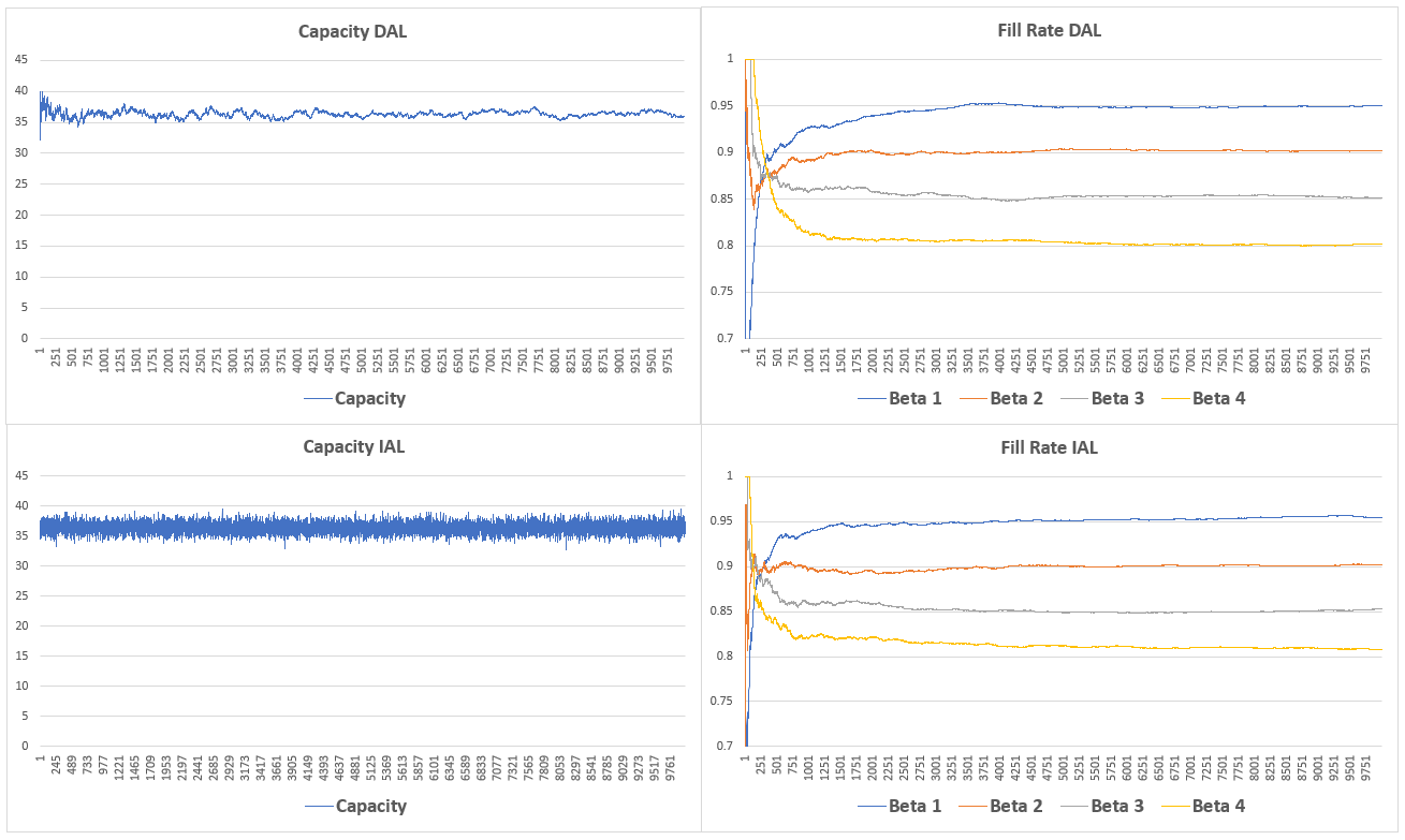
Figure 1: Numerical results of DAL and IAL algorithms with service level (covering) constraints for the stationary case.

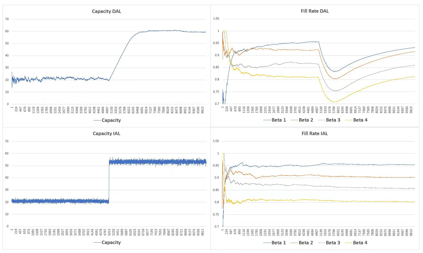
Figure 2: Numerical results of DAL and IAL algorithms with service level (covering) constraints for the non-stationary case 1.

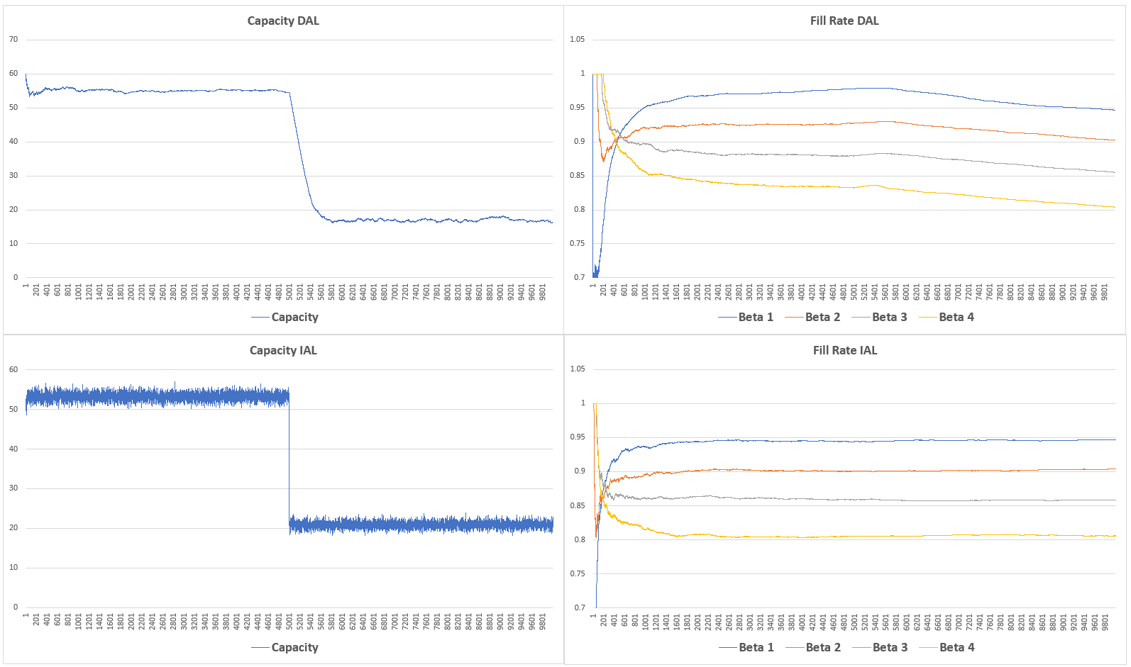
Figure 3: Numerical results of DAL and IAL algorithms with service level (covering) constraints for the non-stationary case 2.

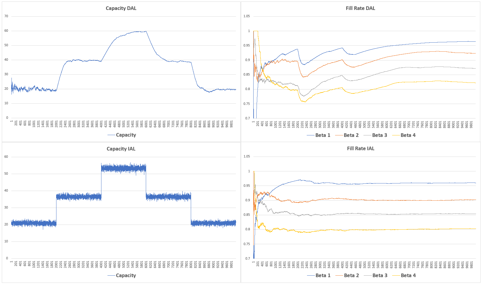
Figure 4: Numerical results of DAL and IAL algorithms with service level (covering) constraints for the non-stationary case 3.

6 Summary

This paper proposes and studies the problem of bounding regret for online two-stage stochastic optimization with long-term constraints. The main contribution is an algorithmic framework that develops new algorithms via adversarial learning algorithms. The framework is applied to various setting. For the stationary setting, the resulted DAL algorithm is shown to achieve a sublinear regret, with a performance robust to adversarial corruptions. For the non-stationary (adversarial) setting, a modified IAL algorithm is developed, with the help of prior estimates. The sublinear regret can also be acheived by IAL algorithm as long as the cumulative inaccuracy of the prior estimates is sublinear.

7 Further Related Literature

Our model synthesizes the bandits-based model, where the representative problems include MAB problem, bandits with knapsack (BwK) problem and the more general OCO problem, and the feature-based model, where the representative problems include online allocation problem and a special case online packing problem. We now review these literature.

One representative problem for the bandits-based model is the BwK problem which reduces to MAB problem if no long-term constraints. The previous BwK results have focused on a stochastic setting [Badanidiyuru et al., 2013, Agrawal and Devanur, 2014a], where a $O(\sqrt{T})$ regret bound has been derived, and an adversarial setting (e.g. Rangi et al. [2018], Immorlica et al. [2019]), where the sublinear regret is impossible to obtain and a $O(\log T)$ competitive ratio has been derived. Similar to our DAL algorithm, the algorithms in the previous literature reply on an interplay between the primal and dual LPs. To be more concrete, Agrawal and Devanur [2014a] and Agrawal and Devanur [2014b] develop a dual-based algorithms to BwK and a more general online stochastic optimization problem (belonging to bandits-based model) and analyzes the algorithm performance under further stronger conditions on the dual optimal solution. However, these learning models and algorithms are developed in the stationary (stochastic) environment, which cannot be applied to the non-stationary setting. For the non-stationary setting, the recent work Liu et al. [2022] derives sublinear regret, based on a more involved complexity measure over the non-stationarity of the underlying distributions which concerns both the temporary changes of two neighborhood distributions and the global changes of the entire distribution sequence.

Another representative problem for the bandits-based model is the OCO problem, which is one of the leading online learning frameworks [Hazan, 2016]. Note that the standard OCO problem generally adopts a static optimal policy as the benchmark, i.e., the decision of the benchmark needs to be the same for each period. In contrast, in our model, the benchmark is a more powerful dynamic optimal policy where the decisions are allowed to be non-homogeneous across time. Therefore, not only our model is more involved, our benchmark is also stronger. There have been results that consider a dynamic optimal policy as the benchmark for OCO [Besbes et al., 2015, Hall and Willett, 2013, Jadbabaie et al., 2015], but all these works consider the unconstrained setting with no long-term constraints. For the line of works that study the problem of online convex optimization with constraints (OCOwC), existing literature would assume the constraint functions that characterize the long-term constraints are either static [Jenatton et al., 2016, Yuan and Lamperski, 2018, Yi et al., 2021] or stochastically generated [Neely and Yu, 2017].

For the type-based model, one representative problem is the online packing problem, where the columns and the corresponding coefficient in the objective of the underlying LP come one by one and the decision has to be made on-the-fly. The packing problem covers a wide range of applications, including secretary problem [Ferguson et al., 1989, Arlotto and Gurvich, 2019], online knapsack problem [Arlotto and Xie, 2020, Jiang and Zhang, 2019], resource allocation problem [Li et al., 2020], network routing problem [Buchbinder and Naor, 2009], matching problem [Mehta et al., 2007] etc. The problem is usually studied under either a stochastic model where the reward and size of each query is drawn independently from an unknown distribution $\mathcal{P}$, or a more general the random permutation model where the queries arrive in a random order [Molinaro and Ravi, 2014, Agrawal et al., 2014, Kesselheim et al., 2014, Gupta and Molinaro, 2014]. The more general online allocation problem (e.g. Balseiro et al. [2022b]) has also been considered in the literature, where the objective and the constraint functions are allowed to be general functions.

8 Extensions

8.1 Non-convex Objective and Non-concave Constraints

Note that in Section 2, we require a convexity condition where the function $p(\cdot)$ is a convex function with $p(\bm{0})=0$ and $\mathcal{C}$ is a compact and convex set which contains $\bm{0}$. Also, the functions $f_{\theta}(\cdot)$ need to be convex in $\bm{x}$ and $\bm{g}_{\theta}(\cdot,\cdot)$ need to be convex in both $\bm{c}$ and $\bm{x}$, for any $\theta$. In this section, we explore whether these convexity conditions can be removed with further characterization of our model.

We now show that when $\mathcal{C}$ contains only a finite number of elements, we can remove all the convexity requirements in Section 2 and we still obtain a $\tilde{O}(\sqrt{T}+W_{T})$ regret bound for the setting in Section 4. As for the setting in Section 3, we can obtain the same $\tilde{O}(\sqrt{T}+W_{T})$ regret bound for arbitrary $\mathcal{C}$, as long as the minimization step $\bm{c}_{t}=\text{argmin}_{\bm{c}\in\mathcal{C}}\hat{L}_{t}(\bm{c},\mu\cdot\bm{e}_{i_{t}})$ can be efficiently solved in Algorithm 1.

We now assume $\mathcal{C}$ has a finite support and remove all the convexity requirements in Section 2. In order to recover the results in Section 4, we regard each element in $\mathcal{C}$ as an expert and we apply expert algorithms to decide $\bm{c}_{t}$ for each period $t$. To be more concrete, note that for the first-stage decision, we only have bandit-feedback, i.e., we can only observe the stochastic outcome of selecting $\bm{c}_{t}$ instead of other elements in the set $\mathcal{C}$. Therefore, we can apply EXP3 algorithm [Auer et al., 2002] as $\mathsf{ALG}_{1}$. Still, following the same procedure as the proof of Theorem 4.3, we can reduce the regret bound of Algorithm 2 into the regret bound of $\mathsf{ALG}_{1}$, $\mathsf{ALG}_{2}$, and an additional $O(W_{T})$ term if adversarial corruption exists. The above argument is formalized in the following theorem.

Theorem 8.1

Denote by $\pi$ Algorithm 2 with input $\mu=T$. Then, if $\mathcal{C}$ constains only a finite number of elements, denoted by $K$, with condition c in Section 2, it holds that

$$\text{Regret}^{\text{c}}(\pi,T)=\mathbb{E}_{\bm{\theta}\sim\bm{P}}[\mathsf{ALG}(\pi,\bm{\theta}^{c})]-\mathbb{E}_{\bm{\theta}\sim\bm{P}}[\mathsf{ALG}(\pi^{*},\bm{\theta}^{c})]\leq \tilde{O}(\sqrt{K\cdot T})+\tilde{O}(\sqrt{T\cdot\log m})$$

$$+O(\mathbb{E}_{\bm{\theta}\sim\bm{P}}[W(\bm{\theta})]),$$ (16)

if EXP3 is selected as $\mathsf{ALG}_{1}$ and Hedge is selected as $\mathsf{ALG}_{2}$. Here, $\mathbb{E}_{\bm{\theta}\sim\bm{P}}[W(\bm{\theta})]$ denotes the expectation of the total number of corruptions, with $W(\bm{\theta})$ defined in (13).

We now consider the setting in Section 3 and we show that the $\tilde{O}(\sqrt{T}+W_{T})$ regret bound holds for Algorithm 1 without the convexity requirements in Section 2, for arbitrary $\mathcal{C}$ as long as the minimization step $\bm{c}_{t}=\text{argmin}_{\bm{c}\in\mathcal{C}}\hat{L}_{t}(\bm{c},\mu\cdot\bm{e}_{i_{t}})$ can be efficiently solved. The key idea is to regard the first-stage decision at each period as a distribution over $\mathcal{C}$, denoted by $\tilde{\bm{c}}_{t}$. Then, $\mathbb{E}_{\tilde{\bm{C}}}\left[\hat{L}(\tilde{\bm{C}},\bm{\lambda})\right]$ would be a convex function over the distribution $\tilde{\bm{C}}$. Moreover, for each fixed $\bm{\lambda}$, note that selecting the worst distribution $\tilde{\bm{C}}$ to minimize $\mathbb{E}_{\tilde{\bm{C}}}\left[\hat{L}(\tilde{\bm{C}},\bm{\lambda})\right]$ can be reduced equivalent to selecting the worst deterministic $\bm{C}$ to minimize $\hat{L}(\bm{C},\bm{\lambda})$. Therefore, every step of the proof of Lemma 3.2 and Theorem 3.3 would follow by replacing $\bm{c}_{t}$ into the distribution $\tilde{\bm{c}}_{t}$ for each $t\in[T]$. We have the following result.

Theorem 8.2

Denote by $\pi$ Algorithm 1 with input $\mu=\|\hat{\bm{\lambda}}^{*}\|_{\infty}=\alpha\cdot T$ for some constant $\alpha>0$. Denote by $W_{T}=\sum_{t=1}^{T}W(\hat{P}_{t},P_{t})$ the total measure of inaccuracy, with $W(\hat{P}_{t},P_{t})$ defined in (4). Then, under condition c of Section 2, for arbitrary $\mathcal{C}$, the regret enjoys the upper bound

$$\text{Regret}(\pi,T)= \mathbb{E}_{\bm{\theta}\sim\bm{P}}[\mathsf{ALG}(\pi,\bm{\theta})]-\mathbb{E}_{\bm{\theta}\sim\bm{P}}[\mathsf{ALG}(\pi^{*},\bm{\theta})]\leq\tilde{O}(\sqrt{T\cdot\log m})+O(W_{T})$$ (17)

if Hedge is selected as $\mathsf{ALG}_{\mathsf{Dual}}$. Moreover, we have

$$\frac{1}{T}\sum_{t=1}^{T}g_{i,\theta_{t}}(\bm{c}_{t},\bm{x}_{t})-\beta_{i}\leq\tilde{O}\left(\sqrt{\frac{\log m}{T}}\right)+O\left(\frac{W_{T}}{T}\right),$$ (18)

for each $i\in[m]$.

8.2 Incorporating Covering Constraints

In this section, we discuss how to incorporate covering constraints into our model. Note that in the previous section, we let the long-term constraints $\frac{1}{T}\cdot\sum_{t=1}^{T}\bm{x}_{t}\in\mathcal{B}(\bm{C},\bm{\theta})$ be characterized as follows,

$$\frac{1}{T}\cdot\sum_{t=1}^{T}\bm{g}_{\theta_{t}}(\bm{c}_{t},\bm{x}_{t})\leq\bm{\beta},$$ (19)

with $\bm{\beta}\in(0,1)^{m}$, which corresponds to packing constraints since both $\bm{g}(\cdot)$ and $\bm{\beta}$ are non-negative. For the case with covering constraints, the long-term constraints $\frac{1}{T}\cdot\sum_{t=1}^{T}\bm{x}_{t}\in\mathcal{B}(\bm{C},\bm{\theta})$ would enjoy the following characterization

$$\frac{1}{T}\cdot\sum_{t=1}^{T}\bm{g}_{\theta_{t}}(\bm{c}_{t},\bm{x}_{t})\geq\bm{\beta},$$ (20)

with $\bm{\beta}\in(0,1)^{m}$. We now show that all our previous results hold for the packing constraints (20), by simply changing the input parameter $\mu$ in Algorithm 2 and Algorithm 1. We illustrate through the stationary setting consiered in Section 4 where $P_{t}=P$ for each $t\in[T]$.

Now, (OPT) enjoys the following new formulation.

$$\mathsf{OPT}^{\mathsf{Covering}}=\min \sum_{t=1}^{T}\mathbb{E}_{\tilde{\bm{c}}_{t},\tilde{\bm{x}}_{t},\theta_{t}}\left[p(\tilde{\bm{c}}_{t})+f_{\theta_{t}}(\tilde{\bm{x}}_{t})\right]$$ (21)

s.t. $$\frac{1}{T}\cdot\sum_{t=1}^{T}\mathbb{E}_{\tilde{\bm{c}}_{t},\tilde{\bm{x}}_{t},\theta_{t}}[\bm{g}_{\theta_{t}}(\tilde{\bm{c}}_{t},\tilde{\bm{x}}_{t})]\geq\bm{\beta}$$

$$\tilde{\bm{x}}_{t}\in\mathcal{K}(\theta_{t},\tilde{\bm{c}}_{t}),\tilde{\bm{c}}_{t}\in\mathcal{C},\forall t.$$

The Lagrangian dual of $\mathsf{OPT}^{\mathsf{Covering}}$ (21) can be formulated as follows.

$$\max_{\bm{\lambda}\geq 0}\min_{\tilde{\bm{c}}_{t}\in\mathcal{C}}\mathsf{L}^{\mathsf{Covering}}(\bm{C},\bm{\lambda})=\sum_{t=1}^{T}\mathbb{E}\left[p(\tilde{\bm{c}}_{t})+\frac{1}{T}\cdot\sum_{i=1}^{m}\lambda_{i}+\min_{\tilde{\bm{x}}_{t}\in\mathcal{K}(\theta_{t},\tilde{\bm{c}}_{t})}f_{\theta_{t}}(\tilde{\bm{x}}_{t})-\sum_{i=1}^{m}\frac{\lambda_{i}\cdot g_{i,\theta_{t}}(\tilde{\bm{c}}_{t},\tilde{\bm{x}}_{t})}{T\cdot\beta_{i}}\right].$$ (22)

Similar to (14), we have the following formulation for $\bar{L}(\bm{c},\bm{\lambda},\theta)$ as the single-period decomposition of $\mathsf{L}^{\mathsf{Covering}}(\bm{C},\bm{\lambda})$.

$$\bar{L}^{\mathsf{Covering}}(\bm{c},\bm{\lambda},\theta)=p(\bm{c})+\frac{1}{T}\cdot\sum_{i=1}^{m}\lambda_{i}+\min_{\bm{x}\in\mathcal{K}(\theta,\bm{c})}\left\{f_{\theta}(\bm{x})-\sum_{i=1}^{m}\frac{\lambda_{i}\cdot g_{i,\theta}(\bm{c},\bm{x})}{T\cdot\beta_{i}}\right\}.$$ (23)

We can obtain the following result.

Lemma 8.3

Under the stationary setting where $P_{t}=P$ for each $t\in[T]$, it holds that

$$\max_{\bm{\lambda}\geq 0}\min_{\tilde{\bm{c}}_{t}\in\mathcal{C}}\mathbb{E}_{\tilde{\bm{C}}}[\mathsf{L}^{\mathsf{Covering}}(\bm{C},\bm{\lambda})]=\max_{\bm{\lambda}\geq 0}\min_{\tilde{\bm{c}}\in\mathcal{C}}T\cdot\mathbb{E}_{\tilde{\bm{c}},\theta\sim P}\left[\bar{L}^{\mathsf{Covering}}(\tilde{\bm{c}},\bm{\lambda},\theta)\right].$$

Therefore, we can still regard solving the dual problem (22) as a procedure of solving the repeated zero-sum games, where player 1 chooses the first-stage decision $\bm{c}_{t}$ and player 2 chooses one long term constraint $i_{t}\in[m]$. We still apply Algorithm 2 with the new definition

$$\bar{L}^{\mathsf{Covering}}_{i}(\bm{c}_{t},\mu\cdot\bm{e}_{i_{t}},\theta_{t})=p(\bm{c}_{t})+\frac{\mu}{T}+f_{\theta_{t}}(\bm{x}_{t})-\frac{\mu\cdot g_{i,\theta_{t}}(\bm{c}_{t},\bm{x}_{t})}{T\cdot\beta_{i}}.$$ (24)

However, in order to incorporate covering constraints, we need to adjust the value of the scaling factor $\mu$ and we only terminate our algorithm after the entire horizon has been run out. In fact, we need an upper bound (arbitrary upper bound suffices) over the $l_{1}$ norm of the optimal dual variable $\bm{\lambda}^{*}$ of (22) to serve as the scaling factor $\mu$ and in practice, we can spend the first $\sqrt{T}$ time periods to construct an upper confidence interval of $\bm{\lambda}^{*}$ to serve as $\mu$ without influencing the order of the regret bound.

Theorem 8.4

Denote by $\pi$ Algorithm 2 with input $\mu$ being an upper bound of $\|\bm{\lambda}^{*}\|_{1}$ where $\bm{\lambda}^{*}$ is the optimal dual variable of (22). Then, under Section 2, $\mu=\alpha\cdot T$ for some constant $\alpha>0$ and if OGD is selected as $\mathsf{ALG}_{1}$ and Hedge is selected as $\mathsf{ALG}_{2}$, the regret enjoys the upper bound

$$\text{Regret}^{\text{TSC}}(\pi,T)\leq\tilde{O}((G+F)\cdot\sqrt{T})+\tilde{O}(\sqrt{T\cdot\log m})$$ (25)

and moreover, we have

$$\beta_{i}-\frac{1}{T}\cdot\sum_{t=1}^{T}g_{i,\theta_{t}}(\bm{c}_{t},\bm{x}_{t})\leq\tilde{O}\left(\frac{G+F}{\alpha\sqrt{T}}\right)+\tilde{O}\left(\frac{\sqrt{\log m}}{\alpha\cdot\sqrt{T}}\right),\leavevmode\nobreak\ \leavevmode\nobreak\ \forall i\in[m].$$ (26)

9 Regret Bounds for Adversarial Learning

In this section, we present the implementation details of two adversarial learning algorithms, OGD and Hedge, that will be used as algorithmic subroutines in our Algorithm 2 and Algorithm 1, as well as their regret analysis.

OGD is an algorithm to be executed in a finite horizon of $T$ periods, and at each period $t$, OGD selects an action $\bm{c}_{t}\in\mathcal{C}$, receives an adversarial chosen cost function $h_{t}(\cdot)$ afterwards, and incurs a cost $h_{t}(\bm{c}_{t})$. OGD is designed to minimize the regret

$$\text{Reg}_{\text{OGD}}(T)=\sum_{t=1}^{T}h_{t}(\bm{c}_{t})-\min_{\bm{c}\in\mathcal{C}}\sum_{t=1}^{T}h_{t}(\bm{c}).$$

The implementation of OGD is described in Algorithm 3. In our problem, $h_{t}=\bar{L}^{\text{ISP}}_{i}(\bm{c}_{t},\mu\cdot\bm{e}_{i_{t}},\theta_{t})$ for ISP and $h_{t}=\bar{L}^{\text{OSP}}_{i}(\bm{c}_{t},\mu\cdot\bm{e}_{i_{t}},\theta_{t})$ for OSP. In order to obtain a subgradient, one can compute the optimal dual variable of the inner minimization problem of (14). For example, the inner minimization problem is

$$\min \leavevmode\nobreak\ \leavevmode\nobreak\ \leavevmode\nobreak\ f_{\theta_{t}}(\bm{x})+\frac{\mu\cdot g_{i_{t},\theta_{t}}(\bm{c},\bm{x})}{T\cdot\beta_{i_{t}}}$$ (27)

s.t. $$\leavevmode\nobreak\ \leavevmode\nobreak\ \leavevmode\nobreak\ B_{\theta_{t}}\bm{x}\leq\bm{c}_{t}$$

$$\leavevmode\nobreak\ \leavevmode\nobreak\ \leavevmode\nobreak\ \bm{x}\geq 0$$

and the Lagrangian dual problem of (27) is

$$\max_{\bm{\gamma}\leq 0}\bm{\gamma}^{\top}\bm{c_{t}}+\min_{\bm{x}\geq 0}f_{\theta_{t}}(\bm{x})-\bm{\gamma}^{\top}B_{\theta_{t}}\bm{x}+\frac{\mu\cdot g_{i_{t},\theta_{t}}(\bm{c}_{t},\bm{x})}{T\cdot\beta_{i_{t}}}.$$

The optimal dual solution $\bm{\gamma}_{t}^{*}$ can be computed from the above minimax problem and we know that

$$\nabla h_{t}(\bm{c}_{t})=\bm{\gamma}_{t}^{*}+\frac{\mu\cdot\nabla_{\bm{c}_{t}}g_{i_{t},\theta_{t}}(\bm{c}_{t},\bm{x})}{T\cdot\beta_{i_{t}}}.$$

Clearly when $\mu=a\cdot T$ for a constant $a>0$, we have $\|\bm{\gamma}_{t}^{*}\|_{2}\leq G$ for some constant $G$ that depends only on (the upper bound of gradients of) $\{f_{\theta},\bm{g}_{\theta}\}_{\forall\theta}$, the minimum positive element of $B_{\theta}$ for all $\theta$, and $\max_{i\in[m]}\{\frac{1}{\beta_{i}}\}$. The regret bound of OGD is as follows.

Theorem 9.1 (Theorem 1 of Zinkevich [2003])

If $\eta_{t}=\frac{1}{\sqrt{t}}$, then it holds that

$$\text{Reg}_{\text{OGD}}(T)\leq O\left((G+F)\cdot\sqrt{T}\right)$$

where $F$ is an upper bound of the diameter of the set $\mathcal{C}$ and $G$ is a constant that depends only on (the upper bound of gradients of) $\{f_{\theta},\bm{g}_{\theta}\}_{\forall\theta}$, the minimum positive element of $B_{\theta}$ for all $\theta$, and $\max_{i\in[m]}\{\frac{1}{\beta_{i}}\}$.

Algorithm 3 Online Gradient Descent (OGD) algorithm

  Input: the step size $\eta_{t}$ for each $t\in[T]$.

  Initially set an arbitrarily $\bm{c}_{1}\in\mathcal{C}$.

  for $t=1,\dots,T$ do

     $\bm{1}.$ Take the action $\bm{c}_{t}$.

     $\bm{2}.$ Observe the cost function $h_{t}(\cdot)$.

     $\bm{3}.$ Update action

$$\bm{c}_{t+1}=\mathcal{P}_{\mathcal{C}}\left(\bm{c}_{t}-\eta_{t}\cdot\nabla h_{t}(\bm{c}_{t})\right)$$

where $\nabla h_{t}(\bm{c}_{t})$ denotes a subgradient of $h_{t}$ at $\bm{c}_{t}$ and $\mathcal{P}_{\mathcal{C}}$ denotes a projection to the set $\mathcal{C}$.

  end for

The Hedge algorithm is used to solve the expert problem in a finite horizon of $T$ periods. There are $m$ experts and at each period $t$, Hedge will select one expert $i_{t}\in[m]$ ($i_{t}$ can be randomly chosen), observe the reward vector $\bm{l}_{t}\in\mathbb{R}^{m}$ afterwards, and obtain an reward $l_{i_{t},t}$. Hedge is designed to minimize the regret

$$\text{Reg}_{\text{Hedge}}(T)=\max_{i\in[m]}\sum_{t=1}^{T}l_{i,t}-\sum_{t=1}^{T}\mathbb{E}_{i_{t}}[l_{i_{t},t}].$$

The Hedge algorithm is described in Algorithm 4. In our problem, for ISP, we have

$$l_{i,t}=\bar{L}_{i}(\bm{c}_{t},\mu\cdot\bm{e}_{i_{t}},\theta_{t}).$$

Under Section 2, when $\mu=\alpha\cdot T$ for a constant $\alpha$, we know that there exists a constant $\delta>0$ such that $|l_{i,t}|\leq\delta$, for all $i\in[m]$ and $t\in[T]$. Here, $\delta$ depends on $\max_{i\in[m]}\{\frac{1}{\beta_{i}}\}$.

Theorem 9.2 (from Theorem 2 in Freund and Schapire [1997])

If $\varepsilon=\sqrt{\frac{\log m}{T}}$, then it holds that

$$\text{Reg}_{\text{Hedge}}(T)\leq\tilde{O}(\sqrt{T\cdot\log(m)})$$

where the constant term in $\tilde{O}(\cdot)$ depends on $\max_{i\in[m]}\{\frac{1}{\beta_{i}}\}$.

Algorithm 4 Hedge algorithm

  Input: a parameter $\varepsilon>0$.

  Initialize: $\bm{w}_{1}=\bm{1}\in\mathbb{R}^{m}$ and $\bm{y}_{1}=\frac{1}{m}\cdot\bm{w}_{1}$.

  for $t=1,\dots,T$ do

     $\bm{1}.$ Take the action $i_{t}\sim\bm{y}_{t}$.

     $\bm{2}.$ Observe the reward vector $\bm{l}_{t}$ and obtain a reward $l_{i_{t},t}$.

     $\bm{3}.$ Update the weight

$$w_{i,t+1}=w_{i,t}\cdot\exp(-\varepsilon\cdot l_{i,t})$$

for each $i\in[m]$ and set

$$y_{i,t+1}=\frac{w_{i,t+1}}{\sum_{i^{\prime}=1}^{m}w_{i^{\prime},t+1}}$$

for each $i\in[m]$.

  end for

10 Missing Proofs for Section 3

Proof of Theorem 3.1.

The proof is modified from the proof of Theorem 4.1. We consider a special case of our problem where for any $\bm{c}\in\mathcal{C}$ and any $\theta$, $\mathcal{K}(\theta,\bm{c})=[0,1]$ (there is no need to decide the first-stage decision). There is only one long-term constraint with target $\beta=\frac{1}{2}$. Moreover, there are three possible values of $\theta$, denoted by $\{\theta^{1},\theta^{2},\theta^{3}\}$. We have $f_{\theta^{1}}(x)=-x$, $f_{\theta^{2}}(x)=-\left(1+\frac{W_{T}}{T}\right)x$, $f_{\theta^{3}}(x)=-\left(1-\frac{W_{T}}{T}\right)x$ and $g_{\theta^{1}}(x)=g_{\theta^{2}}(x)=g_{\theta^{3}}(x)=x$ (only one long-term constraint). The prior estimate is $\hat{P}_{t}=\theta^{1}$ with probability 1 for each $t\in[T]$, and the problem with respect to the prior estimates can be described below in (28).

$$\min\ \ -x_{1}-...-x_{\frac{T}{2}}-x_{\frac{T}{2}+1}-...-x_{T}$$ (28)

s.t. $$x_{1}+...+x_{\frac{T}{2}}+x_{\frac{T}{2}+1}+...+x_{T}\leq\frac{T}{2}$$

$$0\leq x_{t}\leq 1\ \text{ for }t=1,...,T.$$

Now we consider the following two possible true distributions. The first possible true scenario, given in (29), is that the distribution $P_{t}=\theta^{1}$ for $t=1,\dots,\frac{T}{2}$ and $P_{t}=\theta^{2}$ for $t=\frac{T}{2}+1,\dots,T$. The second possible true scenario, given in (30), is that the distribution $P_{t}=\theta^{1}$ for $t=1,\dots,\frac{T}{2}$ and $P^{c}_{t}=\theta^{3}$ for $t=\frac{T}{2}+1,\dots,T$.

$$\min\ \ -x_{1}-...-x_{\frac{T}{2}}-\left(1+\frac{W_{T}}{T}\right)x_{\frac{T}{2}+1}-...-\left(1+\frac{W_{T}}{T}\right)x_{T}$$ (29)

s.t. $$x_{1}+...+x_{\frac{T}{2}}+x_{\frac{T}{2}+1}+...+x_{T}\leq\frac{T}{2}$$

$$0\leq x_{t}\leq 1\ \text{ for }t=1,...,T.$$

$$\min\ \ -x_{1}-...-x_{\frac{T}{2}}-\left(1-\frac{W_{T}}{T}\right)x_{\frac{T}{2}+1}-...-\left(1-\frac{W_{T}}{T}\right)x_{T}$$ (30)

s.t. $$x_{1}+...+x_{\frac{T}{2}}+x_{\frac{T}{2}+1}+...+x_{T}\leq\frac{T}{2}$$

$$0\leq x_{t}\leq 1\ \text{ for }t=1,...,T.$$

For any online policy $\pi$, denote by $x^{1}_{t}(\pi)$ the decision of the policy $\pi$ at period $t$ under the true scenario given in (29) and denote by $x^{2}_{t}(\pi)$ the decision of the policy $\pi$ at period $t$ under the true scenario (30). Further define $T_{1}(\pi)$ (resp. $T_{2}(\pi)$) as the expected capacity consumption of policy $\pi$ under the true scenario (29) (resp. true scenario (30)) during the first $\frac{T}{2}$ time periods:

$$T_{1}(\pi)=\mathbb{E}\left[\sum_{t=1}^{\frac{T}{2}}x^{1}_{t}(\pi)\right]\text{\leavevmode\nobreak\ \leavevmode\nobreak\ \leavevmode\nobreak\ and\leavevmode\nobreak\ \leavevmode\nobreak\ \leavevmode\nobreak\ }T_{2}(\pi)=\mathbb{E}\left[\sum_{t=1}^{\frac{T}{2}}x^{2}_{t}(\pi)\right]$$

Then, we have that

$$\mathsf{ALG}_{T}^{1}(\pi)=-\frac{T+W_{T}}{2}+\frac{W_{T}}{T}\cdot T_{1}(\pi)\text{\leavevmode\nobreak\ \leavevmode\nobreak\ \leavevmode\nobreak\ and\leavevmode\nobreak\ \leavevmode\nobreak\ \leavevmode\nobreak\ }\mathsf{ALG}_{T}^{2}(\pi)=-\frac{T-W_{T}}{2}-\frac{W_{T}}{T}\cdot T_{2}(\pi)$$

where $\mathsf{ALG}_{T}^{1}(\pi)$ (resp. $\mathsf{ALG}_{T}^{2}(\pi)$) denotes the expected reward collected by policy $\pi$ on scenario (29) (resp. scenario (30)). It is clear to see that the optimal policy $\pi^{*}$ who is aware of $P_{t}$ for each $t\in[T]$ can achieve an objective value

$$\mathsf{ALG}_{T}^{1}(\pi^{*})=-\frac{T+W_{T}}{2}\text{\leavevmode\nobreak\ \leavevmode\nobreak\ \leavevmode\nobreak\ and\leavevmode\nobreak\ \leavevmode\nobreak\ \leavevmode\nobreak\ }\mathsf{ALG}_{T}^{2}(\pi^{*})=-\frac{T}{2}.$$

Thus, the regret of policy $\pi$ on scenario (29) and (30) are $\frac{W_{T}}{T}\cdot T_{1}(\pi)$ and $W_{T}-\frac{W_{T}}{T}\cdot T_{2}(\pi)$ respectively. Further note that since the implementation of policy $\pi$ at each time period should be independent of future realizations, we must have $T_{1}(\pi)=T_{2}(\pi)$ (during the first $\frac{T}{2}$ periods, the information for $\pi$ is the same for both scenarios (29) and (30)). Thus, we have that

$$\text{Reg}_{T}(\pi)\geq\max\left\{\frac{W_{T}}{T}\cdot T_{1}(\pi),W_{T}-\frac{W_{T}}{T}\cdot T_{1}(\pi)\right\}\geq\frac{W_{T}}{2}=\Omega(W_{T})$$

which completes our proof. $\Halmos$

Proof of Lemma 3.2.

Denote by $(\hat{\bm{\lambda}}^{*},(\hat{\bm{c}}^{*}_{t})_{t=1}^{T})$ the optimal solution to

$$\max_{\bm{\lambda}\geq 0}\min_{\bm{c}_{t}\in\mathcal{C}}\hat{L}(\bm{C},\bm{\lambda}),$$

used in the definition (6). we now show that $(\hat{\bm{\lambda}}^{*},\hat{\bm{c}}^{*}_{t})$ is an optimal solution to

$$\max_{\bm{\lambda}\geq 0}\min_{\bm{c}_{t}\in\mathcal{C}}\hat{L}_{t}(\bm{c}_{t},\bm{\lambda})$$

for each $t\in[T]$, which would help to complete our proof of (8). We first define

$$L_{t}(\bm{\lambda})=\min_{\bm{c}_{t}\in\mathcal{C}}\hat{L}_{t}(\bm{c}_{t},\bm{\lambda}),$$

as a function over $\bm{\lambda}$ for each $t\in[T]$. Then, it holds that

$$\nabla L_{t}(\hat{\bm{\lambda}}^{*})=\nabla\hat{L}_{t}(\hat{\bm{c}}^{*}_{t},\hat{\bm{\lambda}}^{*})=\left(-\frac{\hat{\beta}_{i,t}}{T\beta_{i}}+\mathbb{E}_{\theta\sim\hat{P}_{t}}\left[\frac{g_{i,\theta}(\hat{\bm{c}}^{*}_{t},\hat{\bm{x}}^{*}_{t}(\theta))}{T\beta_{i}}\right]\right)_{\forall i\in[m]}=\bm{0}$$ (31)

The first equality of (31) follows from the fact that

$$\hat{\bm{c}}^{*}_{t}\in\text{argmin}_{\bm{c}\in\mathcal{C}}\mathbb{E}_{\theta\sim\hat{P}_{t}}\left[p(\bm{c})+\min_{\bm{x}\in\mathcal{K}(\theta,\bm{c})}f_{\theta}(\bm{x})+\sum_{i=1}^{m}\frac{\hat{\lambda}^{*}_{i}\cdot g_{i,\theta}(\bm{c},\bm{x})}{T\cdot\beta_{i}}\right]$$ (32)

since $(\hat{\bm{\lambda}}^{*},(\hat{\bm{c}}^{*}_{t})_{t=1}^{T})$ is an optimal solution to $\max_{\bm{\lambda}\geq 0}\min_{\bm{c}_{t}\in\mathcal{C}}\hat{L}(\bm{C},\bm{\lambda})$. The last equality of (31) follows from the definition of $\hat{\beta}_{i,t}$ in (6). Therefore, combining (31) and (32), we know that $(\hat{\bm{\lambda}}^{*},\hat{\bm{c}}^{*}_{t})$ is an optimal solution to $\max_{\bm{\lambda}\geq 0}\min_{\bm{c}_{t}\in\mathcal{C}}\hat{L}_{t}(\bm{c}_{t},\bm{\lambda})$ for each $t\in[T]$.

We now prove (8). It is sufficient to prove that

$$\hat{L}(\hat{\bm{C}}^{*},\hat{\bm{\lambda}}^{*})=\sum_{t=1}^{T}\hat{L}_{t}(\hat{\bm{c}}^{*}_{t},\hat{\bm{\lambda}}^{*})$$ (33)

where $\hat{\bm{C}}^{*}=(\hat{\bm{c}}^{*}_{t})_{t=1}^{T}$. We define an index set $\mathcal{I}=\{i\in[m]:\hat{\lambda}^{*}_{i}>0\}$. Clearly, for each $i\in\mathcal{I}$, the optimality of $\hat{\bm{\lambda}}^{*}$ would require that

$$\nabla_{\lambda_{i}}\bar{L}(\hat{\bm{C}}^{*},\hat{\bm{\lambda}}^{*})=-1+\frac{1}{T\beta_{i}}\sum_{t=1}^{T}\mathbb{E}_{\theta\sim\hat{P}_{t}}\left[g_{i,\theta}(\hat{\bm{c}}_{t}^{*},\hat{\bm{x}}^{*}_{t}(\theta))\right]=0$$

which implies $\sum_{t=1}^{T}\hat{\beta}_{i,t}=T\cdot\beta$. Therefore, we would have

$$\sum_{i=1}^{m}\sum_{t=1}^{T}\frac{\hat{\lambda}^{*}_{i,t}\hat{\beta}_{i}}{T\beta_{i}}=\sum_{i=1}^{m}\hat{\lambda}^{*}_{i}.$$

which completes our proof of (9) and therefore (8). $\Halmos$

Proof of Theorem 3.3.

The proof can be classified by the following two steps. We denote by

$$\mathsf{L}_{t}(\bm{c},\bm{\lambda}):=\mathbb{E}_{\theta\sim P_{t}}\left[p(\bm{c})-\sum_{i=1}^{m}\frac{\lambda_{i}\cdot\hat{\beta}_{i,t}}{T\cdot\beta_{i}}+\min_{\bm{x}\in\mathcal{K}(\theta,\bm{c})}f_{\theta}(\bm{x})+\sum_{i=1}^{m}\frac{\lambda_{i}\cdot g_{i,\theta}(\bm{c},\bm{x})}{T\cdot\beta_{i}}\right]$$ (34)

for each $t\in[T]$. Our first step is to show that for any $\bm{\lambda}\geq 0$ and any $\bm{c}\in\mathcal{C}$, it holds that

$$\left|\mathsf{L}_{t}(\bm{c},\bm{\lambda})-\hat{L}_{t}(\bm{c},\bm{\lambda})\right|\leq\frac{\|\bm{\lambda}\|_{1}}{T\beta_{\min}}\cdot W(\hat{P}_{t},P_{t})$$ (35)

where $\beta_{\min}=\min_{i\in[m]}\{\beta_{i}\}$.

We now prove (35). We define

$$\hat{L}_{t}(\bm{c},\bm{\lambda},\theta):=p(\bm{c})-\sum_{i=1}^{m}\frac{\lambda_{i}\cdot\hat{\beta}_{i,t}}{T\cdot\beta_{i}}+\min_{\bm{x}\in\mathcal{K}(\theta,\bm{c})}f_{\theta}(\bm{x})+\sum_{i=1}^{m}\frac{\lambda_{i}\cdot g_{i,\theta}(\bm{c},\bm{x})}{T\cdot\beta_{i}}.$$

It is clear to see that

$$\mathsf{L}_{t}(\bm{c},\bm{\lambda})=\mathbb{E}_{\theta\sim P_{t}}\left[\hat{L}_{t}(\bm{c},\bm{\lambda},\theta)\right]\text{\leavevmode\nobreak\ and\leavevmode\nobreak\ }\hat{L}_{t}(\bm{c},\bm{\lambda})=\mathbb{E}_{\theta\sim\hat{P}_{t}}\left[\hat{L}_{t}(\bm{c},\bm{\lambda},\theta)\right].$$

Moreover, note that for any $\theta,\theta^{\prime}$, we have

$$|\hat{L}_{t}(\bm{c},\bm{\lambda},\theta)-\hat{L}_{t}(\bm{c},\bm{\lambda},\theta^{\prime})|\leq\frac{\|\bm{\lambda}\|_{1}}{T\beta_{\min}}\cdot d(\theta,\theta^{\prime}),$$

with $d(\theta,\theta^{\prime})=\|(f_{\theta},\bm{g}_{\theta})-(f_{\theta^{\prime}},\bm{g}_{\theta^{\prime}})\|_{\infty}$ in the definition (4). Therefore, we have

$$\left|\mathsf{L}_{t}(\bm{c},\bm{\lambda})-\hat{L}_{t}(\bm{c},\bm{\lambda})\right|=\left|\mathbb{E}_{\theta\sim P_{t}}\left[\hat{L}_{t}(\bm{c},\bm{\lambda},\theta)\right]-\mathbb{E}_{\theta^{\prime}\sim\hat{P}_{t}}\left[\hat{L}_{t}(\bm{c},\bm{\lambda},\theta^{\prime})\right]\right|\leq\frac{\|\bm{\lambda}\|_{1}}{T\beta_{\min}}\cdot W(\hat{P}_{t},P_{t}),$$

thus, complete our proof of (35).

Our second step is to bound the final regret with the help of (35). We assume without loss of generality that there always exists $i^{\prime}\in[m]$ such that

$$\sum_{t=1}^{T}g_{i^{\prime},\theta_{t}}(\bm{c}_{t},\bm{x}_{t})\geq T\cdot\beta_{i^{\prime}}.$$ (36)

In fact, let there be a dummy constraint $i^{\prime}$ such that $g_{i^{\prime},\theta}(\bm{c},\bm{x})=\beta_{i^{\prime}}=\alpha$, for arbitrary $\alpha\in(0,1)$, for any $\theta$ and $\bm{c},\bm{x}$. Then, (36) holds.

Let $(\hat{\bm{\lambda}}^{*},(\hat{\bm{c}}^{*}_{t})_{t=1}^{T})$ be the optimal solution to $\max_{\bm{\lambda}\geq 0}\min_{\bm{c}_{t}\in\mathcal{C}}\hat{L}(\bm{C},\bm{\lambda})$ used in the definition (6). Then, it holds that

$$\mathbb{E}_{\bm{\theta}\sim\bm{P}}\left[\sum_{t=1}^{T}\hat{L}_{t}(\bm{c}_{t},\mu\cdot\bm{e}_{i_{t}},\theta_{t})\right] =\sum_{t=1}^{T}\mathbb{E}_{\bm{c}_{t},i_{t}}\left[\mathsf{L}_{t}(\bm{c}_{t},\mu\cdot\bm{e}_{i_{t}})\right]$$ (37)

$$\leq\sum_{t=1}^{T}\mathbb{E}_{\bm{c}_{t},i_{t}}\left[\hat{L}_{t}(\bm{c}_{t},\mu\cdot\bm{e}_{i_{t}})\right]+\frac{\mu\cdot W_{T}}{T\beta_{\min}}=\sum_{t=1}^{T}\mathbb{E}_{i_{t}}\left[\min_{\bm{c}\in\mathcal{C}}\hat{L}_{t}(\bm{c},\mu\cdot\bm{e}_{i_{t}})\right]+\frac{\mu\cdot W_{T}}{T\beta_{\min}}$$

$$\leq\sum_{t=1}^{T}\min_{\bm{c}\in\mathcal{C}}\hat{L}_{t}(\bm{c},\hat{\bm{\lambda}}^{*})+\frac{\mu\cdot W_{T}}{T\beta_{\min}}=\sum_{t=1}^{T}\hat{L}_{t}(\hat{\bm{c}}^{*}_{t},\hat{\bm{\lambda}}^{*})+\frac{\mu\cdot W_{T}}{T\beta_{\min}}$$

where the first inequality follows from the definition of $\bm{c}_{t}$, the second inequality follows from Lemma 3.2, and the last equality follows from the definition of $\hat{\bm{c}}^{*}_{t}$.

On the other hand, for any $i\in[m]$, we have

$$\sum_{t=1}^{T}\hat{L}_{t}(\bm{c}_{t},\mu\cdot\bm{e}_{i_{t}},\theta_{t})\geq\sum_{t=1}^{T}\hat{L}_{i,t}(\bm{c}_{t},\mu\cdot\bm{e}_{i_{t}},\theta_{t})-\text{Reg}(T,\bm{\theta})$$

with $\hat{L}_{i,t}$ defined in (11), where $\text{Reg}(\tau,\bm{\theta})$ denotes the regret bound of $\mathsf{ALG}_{\mathsf{Dual}}$ (holds for arbitrary $\bm{\lambda}=\mu\cdot\bm{e}_{i}$). We now denote by

$$i^{*}=\text{argmax}_{i\in[m]}\{\frac{1}{T}\cdot\sum_{t=1}^{T}g_{i,\theta_{t}}(\bm{c}_{t},\bm{x}_{t})-\beta_{i}\}.$$

We also denote by

$$d_{T}(\mathcal{A},\bm{\theta})=\max_{i\in[m]}\{\frac{1}{T}\cdot\sum_{t=1}^{T}g_{i,\theta_{t}}(\bm{c}_{t},\bm{x}_{t})-\beta_{i}\}.$$

From (36), we must have $d_{T}(\mathcal{A},\bm{\theta})\geq 0$. We now set $i=i^{*}$ and we have

$$\sum_{t=1}^{T}\hat{L}_{t}(\bm{c}_{t},\mu\cdot\bm{e}_{i_{t}},\theta_{t}) \geq\sum_{t=1}^{T}\hat{L}_{i^{*},t}(\bm{c}_{t},\mu\cdot\bm{e}_{i_{t}},\theta_{t})-\text{Reg}(T,\bm{\theta})$$ (38)

$$=\sum_{t=1}^{T}\left(p(\bm{c}_{t})+f_{\theta_{t}}(\bm{x}_{t})\right)-\mu\cdot\frac{\sum_{t=1}^{T}\hat{\beta}_{i^{*},t}}{T\beta_{i^{*}}}+\sum_{t=1}^{T}\frac{\mu\cdot g_{i^{*},\theta_{t}}(\bm{c}_{t},\bm{x}_{t})}{T\cdot\beta_{i^{*}}}-\text{Reg}(T,\bm{\theta})$$

From the construction of $\hat{\beta}_{i,t}$, we know that $\sum_{t=1}^{T}\hat{\beta}_{i,t}\leq T\cdot\beta_{i}$ for each $i\in[m]$. To see this point, we note that if we define $\hat{L}(\bm{\lambda})=\min_{\bm{c}_{t}\in\mathcal{C}}\hat{L}(\bm{C},\bm{\lambda})$, then, for each $i\in[m]$,

$$\nabla_{\lambda_{i}}\hat{L}(\hat{\bm{\lambda}}^{*})=-1+\mathbb{E}_{\bm{\theta}\sim\hat{P}}\left[\sum_{t=1}^{T}\frac{g_{i,\theta_{t}}(\hat{\bm{c}}^{*}_{t},\hat{\bm{x}}^{*}(\theta_{t}))}{T\beta_{i}}\right]=-1+\frac{\sum_{t=1}^{T}\hat{\beta}_{i,t}}{T\cdot\beta_{i}}\leq 0.$$ (39)

Otherwise, $\nabla_{\lambda_{i}}\hat{L}(\hat{\bm{\lambda}}^{*})>0$ would violate the optimality of $\hat{\bm{\lambda}}^{*}$ to $\max_{\bm{\lambda}\geq 0}\hat{L}(\bm{\lambda})$.

Plugging (39) into (38), we get

$$\sum_{t=1}^{T}\hat{L}_{t}(\bm{c}_{t},\mu\cdot\bm{e}_{i_{t}},\theta_{t}) \geq\sum_{t=1}^{T}\left(p(\bm{c}_{t})+f_{\theta_{t}}(\bm{x}_{t})\right)-\mu+\sum_{t=1}^{T}\frac{\mu\cdot g_{i^{*},\theta_{t}}(\bm{c}_{t},\bm{x}_{t})}{T\cdot\beta_{i^{*}}}-\text{Reg}(T,\bm{\theta})$$ (40)

$$\geq\sum_{t=1}^{T}\left(p(\bm{c}_{t})+f_{\theta_{t}}(\bm{x}_{t})\right)+\frac{\mu}{\beta_{\min}}\cdot d_{T}(\mathcal{A},\bm{\theta})-\text{Reg}(T,\bm{\theta})$$

Combining (37) and (40), we have

$$\mathbb{E}_{\bm{\theta}\sim\bm{P}}\left[\sum_{t=1}^{T}\left(p(\bm{c}_{t})+f_{\theta_{t}}(\bm{x}_{t})\right)\right]\leq\sum_{t=1}^{T}\hat{L}_{t}(\hat{\bm{c}}^{*}_{t},\hat{\bm{\lambda}}^{*})+\frac{\mu\cdot W_{T}}{T\beta_{\min}}+\mathbb{E}_{\bm{\theta}\sim\bm{P}}\left[\text{Reg}(T,\bm{\theta})\right]-\frac{\mu}{\beta_{\min}}\cdot\mathbb{E}_{\bm{\theta}\sim\bm{P}}\left[d_{T}(\mathcal{A},\bm{\theta})\right].$$ (41)

Denote by $(\bm{\lambda}^{*},\tilde{\bm{C}}^{*})$ the optimal saddle-point solution to

$$\max_{\bm{\lambda}\geq 0}\min_{\tilde{\bm{C}}\in\mathcal{C}}\mathbb{E}_{\tilde{\bm{C}}}[\mathsf{L}(\tilde{\bm{C}},\bm{\lambda})]=\min_{\tilde{\bm{C}}\in\mathcal{C}}\max_{\bm{\lambda}\geq 0}\mathbb{E}_{\tilde{\bm{C}}}[\mathsf{L}(\tilde{\bm{C}},\bm{\lambda})].$$

Then, it holds that

$$\sum_{t=1}^{T}\hat{L}_{t}(\hat{\bm{c}}^{*}_{t},\hat{\bm{\lambda}}^{*}) \leq\sum_{t=1}^{T}\mathbb{E}_{\tilde{\bm{c}}_{t}}[\hat{L}_{t}(\tilde{\bm{c}}^{*}_{t},\hat{\bm{\lambda}}^{*})]\leq\sum_{t=1}^{T}\mathbb{E}_{\tilde{\bm{c}}_{t}}[\mathsf{L}_{t}(\tilde{\bm{c}}^{*}_{t},\hat{\bm{\lambda}}^{*})]+\frac{\|\hat{\bm{\lambda}}^{*}\|_{1}\cdot W_{T}}{T\beta_{\min}}=\mathbb{E}_{\tilde{\bm{C}}}[\mathsf{L}(\tilde{\bm{C}}^{*},\hat{\bm{\lambda}}^{*})]+\frac{\|\hat{\bm{\lambda}}^{*}\|_{1}\cdot W_{T}}{T\beta_{\min}}$$

$$\leq\mathbb{E}_{\tilde{\bm{C}}}[\mathsf{L}(\tilde{\bm{C}}^{*},\hat{\bm{\lambda}}^{*})]+\frac{\|\hat{\bm{\lambda}}^{*}\|_{1}\cdot W_{T}}{T\beta_{\min}}=\mathsf{OPT}+\frac{\|\hat{\bm{\lambda}}^{*}\|_{1}\cdot W_{T}}{T\beta_{\min}},$$ (42)

where the first inequality follows from definition of $(\hat{\bm{\lambda}^{*}},(\hat{\bm{c}}_{t})_{t=1}^{T})$, the second inequality follows from (35), the first equality follows from (9) and the third inequality follows from the saddle-point condition of $(\bm{\lambda}^{*},\tilde{\bm{C}}^{*})$.

Plugging (42) into (41), we have

$$\mathbb{E}_{\bm{\theta}\sim\bm{P}}\left[\sum_{t=1}^{T}\left(p(\bm{c}_{t})+f_{\theta_{t}}(\bm{x}_{t})\right)\right]\leq\mathsf{OPT}+\frac{2\mu W_{T}}{T\beta_{\min}}+\mathbb{E}_{\bm{\theta}\sim\bm{P}}\left[\text{Reg}(T,\bm{\theta})\right]-\frac{\mu}{\beta_{\min}}\cdot\mathbb{E}_{\bm{\theta}\sim\bm{P}}\left[d_{T}(\mathcal{A},\bm{\theta})\right].$$ (43)

with $\mu=\|\hat{\bm{\lambda}}^{*}\|_{1}$. From the non-negativity of $d_{T}(\mathcal{A},\bm{\theta})$, we have

$$\mathbb{E}_{\bm{\theta}\sim\bm{P}}\left[\sum_{t=1}^{T}\left(p(\bm{c}_{t})+f_{\theta_{t}}(\bm{x}_{t})\right)\right]\leq\mathsf{OPT}+\frac{2\mu W_{T}}{T\beta_{\min}}+\mathbb{E}_{\bm{\theta}\sim\bm{P}}\left[\text{Reg}(T,\bm{\theta})\right].$$

Using Theorem 9.2 to bound $\mathbb{E}_{\bm{\theta}\sim\bm{P}}\left[\text{Reg}(T,\bm{\theta})\right]$, we have

$$\mathbb{E}_{\bm{\theta}\sim\bm{P}}\left[\sum_{t=1}^{T}\left(p(\bm{c}_{t})+f_{\theta_{t}}(\bm{x}_{t})\right)\right]\leq\mathsf{OPT}+\frac{2\mu W_{T}}{T\beta_{\min}}+\tilde{O}(\sqrt{T\cdot\log m})$$

which completes our proof of (12) by noting that $\mu=\alpha\cdot T$ for some constant $\alpha>0$.

We note that $(\bm{c}_{t},\bm{x}_{t})_{t=1}^{T}$ defines a feasible solution to

$$\mathsf{OPT}^{\delta}=\min \sum_{t=1}^{T}\mathbb{E}_{\bm{c}_{t},\bm{x}_{t},\theta_{t}\sim P_{t}}\left[p(\bm{c}_{t})+f_{\theta_{t}}(\bm{x}_{t})\right]$$ (44)

s.t. $$\frac{1}{T}\cdot\sum_{t=1}^{T}\mathbb{E}_{\bm{c}_{t},\bm{x}_{t},\theta_{t}\sim P_{t}}[\bm{g}_{\theta_{t}}(\bm{c}_{t},\bm{x}_{t})]\leq\bm{\beta}+\delta\cdot\bm{e}$$

$$\bm{x}_{t}\in\mathcal{K}(\theta_{t},\bm{c}_{t}),\bm{c}_{t}\in\mathcal{C},\forall t.$$

with $\delta=\mathbb{E}_{\bm{\theta}\sim\bm{P}}[d_{T}(\mathcal{A},\bm{\theta})]$ and $\bm{e}$ denotes a vector of all ones. We define another optimization problem by changing $P_{t}$ into $\hat{P}_{t}$ for each $t$,

$$\hat{\mathsf{OPT}}^{\hat{\delta}}=\min \sum_{t=1}^{T}\mathbb{E}_{\bm{c}_{t},\bm{x}_{t},\theta_{t}\sim\hat{P}_{t}}\left[p(\bm{c}_{t})+f_{\theta_{t}}(\bm{x}_{t})\right]$$ (45)

s.t. $$\frac{1}{T}\cdot\sum_{t=1}^{T}\mathbb{E}_{\bm{c}_{t},\bm{x}_{t},\theta_{t}\sim\hat{P}_{t}}[\bm{g}_{\theta_{t}}(\bm{c}_{t},\bm{x}_{t})]\leq\bm{\beta}+\hat{\delta}\cdot\bm{e}$$

$$\bm{x}_{t}\in\mathcal{K}(\theta_{t},\bm{c}_{t}),\bm{c}_{t}\in\mathcal{C},\forall t.$$

We have the following result that bounds the gap between $\mathsf{OPT}^{\delta}$ and $\hat{\mathsf{OPT}}^{\hat{\delta}}$, for some specific $\delta$ and $\hat{\delta}$.

Claim 1

For any $\delta\geq 0$, if we set $\hat{\delta}=\delta+\frac{W_{T}}{T}$, then we have

$$\hat{\mathsf{OPT}}^{\hat{\delta}}\leq\mathsf{OPT}^{\delta}+W_{T}.$$

If we regard $\hat{\mathsf{OPT}}^{\hat{\delta}}$ as a function over $\hat{\delta}$, then $\hat{\mathsf{OPT}}^{\hat{\delta}}$ is clearly a convex function over $\hat{\delta}$, where the proof follows the same spirit as the proof of Lemma 4.2. Moreover, note that

$$\frac{d\hat{\mathsf{OPT}}^{\hat{\delta}=0}}{d\hat{\delta}}=\|\hat{\bm{\lambda}}^{*}\|_{1}\leq\mu.$$

We have

$$\hat{\mathsf{OPT}}=\hat{\mathsf{OPT}}^{0}\leq\hat{\mathsf{OPT}}^{\hat{\delta}}+\mu\cdot\hat{\delta}$$

for any $\hat{\delta}\geq 0$. On the other hand, we have

$$\hat{\mathsf{OPT}}=\max_{\bm{\lambda}\geq 0}\min_{\bm{c}_{t}\in\mathcal{C}}\hat{L}(\bm{C},\bm{\lambda})=\sum_{t=1}^{T}\hat{L}_{t}(\hat{\bm{c}}^{*}_{t},\hat{\bm{\lambda}}^{*})$$ (46)

where the last equality follows from Lemma 3.2. Therefore, we now assume that $\mathbb{E}_{\bm{\theta}\sim\bm{P}}[d_{T}(\mathcal{A},\bm{\theta})]\geq\frac{W_{T}}{T}$, otherwise (3.3) directly holds. We have

$$\sum_{t=1}^{T}\hat{L}_{t}(\hat{\bm{c}}^{*}_{t},\hat{\bm{\lambda}}^{*}) =\hat{\mathsf{OPT}}\leq\hat{\mathsf{OPT}}^{\mathbb{E}_{\bm{\theta}\sim\bm{P}}[d_{T}(\mathcal{A},\bm{\theta})]+\frac{W_{T}}{T}}+\mu\cdot\left(\mathbb{E}_{\bm{\theta}\sim\bm{P}}[d_{T}(\mathcal{A},\bm{\theta})]+\frac{W_{T}}{T}\right)$$ (47)

$$\leq\mathsf{OPT}^{\mathbb{E}_{\bm{\theta}\sim\bm{P}}[d_{T}(\mathcal{A},\bm{\theta})]}+\mu\cdot\mathbb{E}_{\bm{\theta}\sim\bm{P}}[d_{T}(\mathcal{A},\bm{\theta})]+W_{T}\cdot(1+\frac{\mu}{T})$$

$$\leq\sum_{t=1}^{T}\mathbb{E}_{\bm{\theta}\sim\bm{P}}\left[p(\bm{c}_{t})+f_{\theta_{t}}(\bm{x}_{t})\right]+\mu\cdot\mathbb{E}_{\bm{\theta}\sim\bm{P}}[d_{T}(\mathcal{A},\bm{\theta})]+W_{T}\cdot(1+\frac{\mu}{T})$$

where the second inequality follows from 1 by setting $\delta=\mathbb{E}_{\bm{\theta}\sim\bm{P}}[d_{T}(\mathcal{A},\bm{\theta})]$. Plugging (47) into (41), we have

$$\sum_{t=1}^{T}\hat{L}_{t}(\hat{\bm{c}}^{*}_{t},\hat{\bm{\lambda}}^{*})\leq \sum_{t=1}^{T}\hat{L}_{t}(\hat{\bm{c}}^{*}_{t},\hat{\bm{\lambda}}^{*})+\frac{\mu\cdot W_{T}}{T\beta_{\min}}+\mathbb{E}_{\bm{\theta}\sim\bm{P}}\left[\text{Reg}(T,\bm{\theta})\right]-\frac{\mu}{\beta_{\min}}\cdot\mathbb{E}_{\bm{\theta}\sim\bm{P}}\left[d_{T}(\mathcal{A},\bm{\theta})\right]$$

$$+\mu\cdot\mathbb{E}_{\bm{\theta}\sim\bm{P}}[d_{T}(\mathcal{A},\bm{\theta})]+W_{T}\cdot(1+\frac{\mu}{T}),$$

which implies

$$\mu\cdot\left(\frac{1}{\beta_{\min}}-1\right)\cdot\mathbb{E}_{\bm{\theta}\sim\bm{P}}[d_{T}(\mathcal{A},\bm{\theta})]\leq\mathbb{E}_{\bm{\theta}\sim\bm{P}}\left[\text{Reg}(T,\bm{\theta})\right]+\frac{2\mu W_{T}}{T\beta_{\min}}++W_{T}\cdot(1+\frac{\mu}{T}).$$

which completes our final proof by noting that $\mu=\alpha\cdot T$ for some constant $\alpha>0$. $\Halmos$

Proof of 1.

Denote by $(\tilde{\bm{c}}_{t},\tilde{\bm{x}}_{t})_{t=1}^{T}$ one optimal solution to $\mathsf{OPT}^{\delta}$. Then, from the definition of $W_{T}$, we have that

$$\frac{1}{T}\cdot\sum_{t=1}^{T}\mathbb{E}_{\tilde{\bm{c}}_{t},\tilde{\bm{x}}_{t},\theta_{t}\sim\hat{P}_{t}}[\bm{g}_{\theta_{t}}(\bm{c}_{t},\bm{x}_{t})]\leq\frac{1}{T}\cdot\sum_{t=1}^{T}\mathbb{E}_{\tilde{\bm{c}}_{t},\tilde{\bm{x}}_{t},\theta_{t}\sim P_{t}}[\bm{g}_{\theta_{t}}(\bm{c}_{t},\bm{x}_{t})]+\frac{W_{T}}{T}.$$

Therefore, we know that $(\tilde{\bm{c}}_{t},\tilde{\bm{x}}_{t})_{t=1}^{T}$ is a feasible solution to $\hat{\mathsf{OPT}}^{\hat{\delta}}$. On the other hand, from the definition of $W_{T}$, we know that

$$\hat{\mathsf{OPT}}^{\hat{\delta}}\leq\sum_{t=1}^{T}\mathbb{E}_{\tilde{\bm{c}}_{t},\tilde{\bm{x}}_{t},\theta_{t}\sim\hat{P}_{t}}\left[p(\tilde{\bm{c}}_{t})+f_{\theta_{t}}(\tilde{\bm{x}}_{t})\right]\leq\sum_{t=1}^{T}\mathbb{E}_{\tilde{\bm{c}}_{t},\tilde{\bm{x}}_{t},\theta_{t}\sim\hat{P}_{t}}\left[p(\tilde{\bm{c}}_{t})+f_{\theta_{t}}(\tilde{\bm{x}}_{t})\right]+W_{T}=\mathsf{OPT}^{\delta}+W_{T}$$

by noting that the distribution of $\tilde{\bm{c}}_{t}$ must be independent of $\theta_{t}$ for each $t$, which completes our proof. $\Halmos$

11 Missing Proofs for Section 4

Proof of Theorem 4.1.

The proof is modified from the proof of Theorem 2 in Jiang et al. [2020]. We let $W_{T}=\mathbb{E}_{\bm{\theta}\sim\bm{P}}[W(\bm{\theta})]$. We consider a special case of our problem where for any $\bm{c}\in\mathcal{C}$ and any $\theta$, $\mathcal{K}(\theta,\bm{c})=[0,1]$ (there is no need to decide the first-stage decision). There is only one long-term constraint with target $\beta=\frac{1}{2}$. Moreover, there are three possible values of $\theta$, denoted by $\{\theta^{1},\theta^{2},\theta^{3}\}$. We have $f_{\theta^{1}}(x)=-x$, $f_{\theta^{2}}(x)=-\left(1+\frac{W_{T}}{T}\right)x$, $f_{\theta^{3}}(x)=-\left(1-\frac{W_{T}}{T}\right)x$ and $g_{\theta^{1}}(x)=g_{\theta^{2}}(x)=g_{\theta^{3}}(x)=x$ (only one long-term constraint). The true distribution is $P_{t}=\theta^{1}$ with probability 1 for each $t\in[T]$, and the problem with respect to the true distributions can be described below in (48).

$$\min\ \ -x_{1}-...-x_{\frac{T}{2}}-x_{\frac{T}{2}+1}-...-x_{T}$$ (48)

s.t. $$x_{1}+...+x_{\frac{T}{2}}+x_{\frac{T}{2}+1}+...+x_{T}\leq\frac{T}{2}$$

$$0\leq x_{t}\leq 1\ \text{ for }t=1,...,T.$$

Now we consider the following two possible adversarial corruptions. The first possible corruption, given in (49), is that the distribution $P^{c}_{t}=\theta^{2}$ for $t=\frac{T}{2}+1,\dots,T$. The second possible corruption, given in (50), is that the distribution $P^{c}_{t}=\theta^{3}$ for $t=\frac{T}{2}+1,\dots,T$.

$$\min\ \ -x_{1}-...-x_{\frac{T}{2}}-\left(1+\frac{W_{T}}{T}\right)x_{\frac{T}{2}+1}-...-\left(1+\frac{W_{T}}{T}\right)x_{T}$$ (49)

s.t. $$x_{1}+...+x_{\frac{T}{2}}+x_{\frac{T}{2}+1}+...+x_{T}\leq\frac{T}{2}$$

$$0\leq x_{t}\leq 1\ \text{ for }t=1,...,T.$$

$$\min\ \ -x_{1}-...-x_{\frac{T}{2}}-\left(1-\frac{W_{T}}{T}\right)x_{\frac{T}{2}+1}-...-\left(1-\frac{W_{T}}{T}\right)x_{T}$$ (50)

s.t. $$x_{1}+...+x_{\frac{T}{2}}+x_{\frac{T}{2}+1}+...+x_{T}\leq\frac{T}{2}$$

$$0\leq x_{t}\leq 1\ \text{ for }t=1,...,T.$$

For any online policy $\pi$, denote by $x^{1}_{t}(\pi)$ the decision of the policy $\pi$ at period $t$ under corruption scenario given in (49) and denote by $x^{2}_{t}(\pi)$ the decision of the policy $\pi$ at period $t$ under corruption scenario (50). Further define $T_{1}(\pi)$ (resp. $T_{2}(\pi)$) as the expected capacity consumption of policy $\pi$ under corruption scenario (49) (resp. corruption scenario (50)) during the first $\frac{T}{2}$ time periods:

$$T_{1}(\pi)=\mathbb{E}\left[\sum_{t=1}^{\frac{T}{2}}x^{1}_{t}(\pi)\right]\text{\leavevmode\nobreak\ \leavevmode\nobreak\ \leavevmode\nobreak\ and\leavevmode\nobreak\ \leavevmode\nobreak\ \leavevmode\nobreak\ }T_{2}(\pi)=\mathbb{E}\left[\sum_{t=1}^{\frac{T}{2}}x^{2}_{t}(\pi)\right]$$

Then, we have that

$$\mathsf{ALG}_{T}^{1}(\pi)=-\frac{T+W_{T}}{2}+\frac{W_{T}}{T}\cdot T_{1}(\pi)\text{\leavevmode\nobreak\ \leavevmode\nobreak\ \leavevmode\nobreak\ and\leavevmode\nobreak\ \leavevmode\nobreak\ \leavevmode\nobreak\ }\mathsf{ALG}_{T}^{2}(\pi)=-\frac{T-W_{T}}{2}-\frac{W_{T}}{T}\cdot T_{2}(\pi)$$

where $\mathsf{ALG}_{T}^{1}(\pi)$ (resp. $\mathsf{ALG}_{T}^{2}(\pi)$) denotes the expected reward collected by policy $\pi$ on scenario (49) (resp. scenario (50)). It is clear to see that the optimal policy $\pi^{*}$ who is aware of $P^{c}_{t}$ for each $t\in[T]$ can achieve an objective value

$$\mathsf{ALG}_{T}^{1}(\pi^{*})=-\frac{T+W_{T}}{2}\text{\leavevmode\nobreak\ \leavevmode\nobreak\ \leavevmode\nobreak\ and\leavevmode\nobreak\ \leavevmode\nobreak\ \leavevmode\nobreak\ }\mathsf{ALG}_{T}^{2}(\pi^{*})=-\frac{T}{2}.$$

Thus, the regret of policy $\pi$ on scenario (49) and (50) are $\frac{W_{T}}{T}\cdot T_{1}(\pi)$ and $W_{T}-\frac{W_{T}}{T}\cdot T_{2}(\pi)$ respectively. Further note that since the implementation of policy $\pi$ at each time period should be independent of future realizations, and more importantly, should independent of corruptions in the future, we must have $T_{1}(\pi)=T_{2}(\pi)$ (during the first $\frac{T}{2}$ periods, the information for $\pi$ is the same for both scenarios (49) and (50)). Thus, we have that

$$\text{Reg}_{T}(\pi)\geq\max\left\{\frac{W_{T}}{T}\cdot T_{1}(\pi),W_{T}-\frac{W_{T}}{T}\cdot T_{1}(\pi)\right\}\geq\frac{W_{T}}{2}=\Omega(W_{T})$$

which completes our proof. $\Halmos$

Proof of Lemma 4.2.

Fix arbitrary $\bm{\lambda},\theta$, for any $\bm{c}_{1},\bm{c}_{2}\in\mathcal{C}$ and any $\alpha_{1},\alpha_{2}\geq 0$ such that $\alpha_{1}+\alpha_{2}=1$, we prove

$$\alpha_{1}\cdot\bar{L}(\bm{c}_{1},\bm{\lambda},\theta)+\alpha_{2}\cdot\bar{L}(\bm{c}_{2},\bm{\lambda},\theta)\geq\bar{L}(\alpha_{1}\cdot\bm{c}_{1}+\alpha_{2}\cdot\bm{c}_{2},\bm{\lambda},\theta).$$

Now, for $\bar{L}(\bm{c}_{1},\bm{\lambda},\theta)$, we denote by $\bm{x}_{1}^{*}(\theta)$ one optimal solution of the inner minimization problem in the definition of $\bar{L}(\bm{c}_{1},\bm{\lambda},\theta)$ (14). Similarly, for $\bar{L}(\bm{c}_{2},\bm{\lambda},\theta)$, we denote by $\bm{x}_{2}^{*}(\theta)$ one optimal solution of the inner minimization problem in the definition of $\bar{L}(\bm{c}_{2},\bm{\lambda},\theta)$ (14). We then define

$$\bm{x}^{*}_{3}(\theta)=\alpha_{1}\cdot\bm{x}^{*}_{1}(\theta)+\alpha_{2}\cdot\bm{x}^{*}_{2}(\theta),\leavevmode\nobreak\ \leavevmode\nobreak\ \forall\theta.$$

Under Section 2, from the convexity of $f_{\theta}(\cdot)$ and $\bm{g}_{\theta}(\cdot)$, it holds that

$$\alpha_{1}\cdot\left(f_{\theta}(\bm{x}^{*}_{1}(\theta))+\sum_{i=1}^{m}\frac{\lambda_{i}\cdot g_{i,\theta}(\bm{c}_{1},\bm{x}^{*}_{1}(\theta))}{T\cdot\beta_{i}}\right)+\alpha_{2}\cdot\left(f_{\theta}(\bm{x}^{*}_{2}(\theta))+\sum_{i=1}^{m}\frac{\lambda_{i}\cdot g_{i,\theta}(\bm{c}_{2},\bm{x}^{*}_{2}(\theta))}{T\cdot\beta_{i}}\right)$$

$$\geq f_{\theta}(\bm{x}^{*}_{3}(\theta))+\sum_{i=1}^{m}\frac{\lambda_{i}\cdot g_{i,\theta}(\bm{c}_{3},\bm{x}^{*}_{3}(\theta))}{T\cdot\beta_{i}}.$$

with $\bm{c}_{3}=\alpha_{1}\cdot\bm{c}_{1}+\alpha_{2}\cdot\bm{c}_{2}$. Given the convexity of $p(\cdot)$, we have

$$\alpha_{1}\cdot\bar{L}(\bm{c}_{1},\bm{\lambda},\theta)+\alpha_{2}\cdot\bar{L}(\bm{c}_{2},\bm{\lambda},\theta)$$

$$= \alpha_{1}p(\bm{c}_{1})+\alpha_{2}p(\bm{c}_{2})-\frac{1}{T}\sum_{i=1}^{m}\lambda_{i}+\alpha_{1}\left(f_{\theta}(\bm{x}^{*}_{1}(\theta))+\sum_{i=1}^{m}\frac{\lambda_{i}\cdot g_{i,\theta}(\bm{c}_{1},\bm{x}^{*}_{1}(\theta))}{T\cdot\beta_{i}}\right)$$

$$+\alpha_{2}\left(f_{\theta}(\bm{x}^{*}_{2}(\theta))+\sum_{i=1}^{m}\frac{\lambda_{i}\cdot g_{i,\theta}(\bm{c}_{2},\bm{x}^{*}_{2}(\theta))}{T\cdot\beta_{i}}\right)$$

$$\geq p(\alpha_{1}\bm{c}_{1}+\alpha_{2}\bm{c}_{2})+f_{\theta}(\bm{x}^{*}_{3}(\theta))+\sum_{i=1}^{m}\frac{\lambda_{i}\cdot g_{i,\theta}(\bm{c}_{3},\bm{x}^{*}_{3}(\theta))}{T\cdot\beta_{i}}$$

$$\geq \bar{L}(\bm{c}_{3},\bm{\lambda},\theta)$$

where the last inequality follows from $\bm{x}^{*}_{3}(\theta)\in\mathcal{K}(\theta,\bm{c}_{3})$, given the exact formulation of $\mathcal{K}(\theta,\bm{c})$ under Section 2. $\Halmos$

Proof of Theorem 4.3.

Denote by $\tau$ the time period that Algorithm 2 is terminated. There must be a constraint $i^{\prime}\in[m]$ such that

$$\sum_{t=1}^{\tau}g_{i^{\prime},\theta^{c}_{t}}(\bm{c}_{t},\bm{x}_{t})\geq T\cdot\beta_{i^{\prime}}.$$ (51)

Otherwise, we can assume without loss of generality that there exists a dummy constraint $i^{\prime}$ such that $g_{i^{\prime},\theta}(\bm{c}_{t},\bm{x})=\beta_{i^{\prime}}=\alpha$, for arbitrary $\alpha\in(0,1)$, for any $\theta$ and $\bm{c},\bm{x}$. In this case, we can set $\tau=T$.

We denote by $(\bm{\lambda}^{*},\tilde{\bm{c}}^{*})$ one saddle-point optimal solution to

$$\max_{\bm{\lambda}\geq 0}\min_{\tilde{\bm{c}}\in\mathcal{C}}\mathbb{E}_{\tilde{\bm{c}}^{*},\theta\sim P^{c}}\left[\bar{L}(\tilde{\bm{c}},\bm{\lambda},\theta)\right]=\min_{\tilde{\bm{c}}\in\mathcal{C}}\max_{\bm{\lambda}\geq 0}\mathbb{E}_{\tilde{\bm{c}}^{*},\theta\sim P^{c}}\left[\bar{L}(\tilde{\bm{c}},\bm{\lambda},\theta)\right]$$

where $P^{c}$ denotes the uniform mixture of the distributions of $\{\theta^{c}_{t}\}$ for $t=1$ to $\tau$ and the equality follows from the concavity over $\bm{\lambda}$ and the convexity over $\bm{c}$ proved in Lemma 4.2. We have

$$\sum_{t=1}^{\tau}\bar{L}(\bm{c}_{t},\mu\cdot\bm{e}_{i_{t}},\theta^{c}_{t})\leq\sum_{t=1}^{\tau}\mathbb{E}_{\tilde{\bm{c}}^{*}}\left[\bar{L}(\tilde{\bm{c}}^{*},\mu\cdot\bm{e}_{i_{t}},\theta^{c}_{t})\right]+\text{Reg}_{1}(\tau,\bm{\theta}^{c})$$

following regret bound of $\mathsf{ALG}_{1}$. Then, it holds that

$$\mathbb{E}_{\bm{\theta}\sim\bm{P}}\left[\sum_{t=1}^{\tau}\bar{L}(\bm{c}_{t},\mu\cdot\bm{e}_{i_{t}},\theta^{c}_{t})\right] \leq\mathbb{E}_{\tilde{\bm{c}}^{*},\bm{\theta}\sim\bm{P}}\left[\sum_{t=1}^{\tau}\bar{L}(\tilde{\bm{c}}^{*},\mu\cdot\bm{e}_{i_{t}},\theta^{c}_{t})\right]+\mathbb{E}_{\bm{\theta}\sim\bm{P}}\left[\text{Reg}_{1}(\tau,\bm{\theta}^{c})\right]$$ (52)

$$\leq\tau\cdot\mathbb{E}_{\tilde{\bm{c}}^{*},\theta\sim P^{c}}\left[\bar{L}(\tilde{\bm{c}}^{*},\bm{\lambda}^{*},\theta)\right]+\mathbb{E}_{\bm{\theta}\sim\bm{P}}\left[\text{Reg}_{1}(\tau,\bm{\theta}^{c})\right]$$

$$\leq\tau\cdot\mathbb{E}_{\tilde{\bm{c}}^{*},\theta\sim P}\left[\bar{L}(\tilde{\bm{c}}^{*},\bm{\lambda}^{*},\theta)\right]+\mathbb{E}_{\bm{\theta}\sim\bm{P}}\left[\text{Reg}_{1}(\tau,\bm{\theta}^{c})\right]+O(\mathbb{E}_{\bm{\theta}\sim\bm{P}}[W(\bm{\theta})]).$$

On the other hand, for any $i\in[m]$, we have

$$\sum_{t=1}^{\tau}\bar{L}(\bm{c}_{t},\mu\cdot\bm{e}_{i_{t}},\theta^{c}_{t})\geq\sum_{t=1}^{\tau}\bar{L}_{i}(\bm{c}_{t},\mu\cdot\bm{e}_{i_{t}},\theta^{c}_{t})-\text{Reg}_{2}(\tau,\bm{\theta}^{c})$$

following the regret bound of $\mathsf{ALG}_{2}$ (holds for arbitrary $\bm{\lambda}=\mu\cdot\bm{e}_{i}$). We now set $i=i^{\prime}$ and we have

$$\sum_{t=1}^{\tau}\bar{L}(\bm{c}_{t},\mu\cdot\bm{e}_{i_{t}},\theta^{c}_{t}) \geq\sum_{t=1}^{\tau}\bar{L}_{i^{\prime}}(\bm{c}_{t},\mu\cdot\bm{e}_{i_{t}},\theta^{c}_{t})-\text{Reg}_{2}(\tau,\bm{\theta}^{c})$$

$$=\sum_{t=1}^{\tau}\left(p(\bm{c}_{t})+f_{\theta^{c}_{t}}(\bm{x}_{t})\right)-\mu\cdot\frac{\tau}{T}+\sum_{t=1}^{\tau}\frac{\mu\cdot g_{i^{\prime},\theta^{c}_{t}}(\bm{c}_{t},\bm{x}_{t})}{T\cdot\beta_{i^{\prime}}}-\text{Reg}_{2}(\tau,\bm{\theta}^{c})$$

$$\geq\sum_{t=1}^{\tau}\left(p(\bm{c}_{t})+f_{\theta^{c}_{t}}(\bm{x}_{t})\right)+\mu\cdot\frac{T-\tau}{T}-\text{Reg}_{2}(\tau,\bm{\theta}^{c})$$

where the last inequality follows from (51). Then, it holds that

$$\mathbb{E}_{\bm{\theta}\sim\bm{P}}\left[\sum_{t=1}^{\tau}\bar{L}(\bm{c}_{t},\mu\cdot\bm{e}_{i_{t}},\theta^{c}_{t})\right]\geq\mathbb{E}_{\bm{\theta}\sim\bm{P}}\left[\sum_{t=1}^{\tau}\left(p(\bm{c}_{t})+f_{\theta^{c}_{t}}(\bm{x}_{t})\right)\right]+\mu\cdot\frac{T-\tau}{T}-\mathbb{E}_{\bm{\theta}\sim\bm{P}}\left[\text{Reg}_{2}(\tau,\bm{\theta}^{c})\right].$$ (53)

Combining (52) and (53), we have

$$\mathbb{E}_{\bm{\theta}\sim\bm{P}}\left[\sum_{t=1}^{\tau}\left(p(\bm{c}_{t})+f_{\theta^{c}_{t}}(\bm{x}_{t})\right)\right]\leq -\mu\cdot\frac{T-\tau}{T}+\tau\cdot\mathbb{E}_{\tilde{\bm{c}}^{*},\theta\sim P}\left[\bar{L}(\tilde{\bm{c}}^{*},\bm{\lambda}^{*},\theta)\right]+O(\mathbb{E}_{\bm{\theta}\sim\bm{P}}[W(\bm{\theta})])$$

$$+\mathbb{E}_{\bm{\theta}\sim\bm{P}}\left[\text{Reg}_{1}(\tau,\bm{\theta})\right]+\mathbb{E}_{\bm{\theta}\sim\bm{P}}\left[\text{Reg}_{2}(\tau,\bm{\theta})\right].$$

From the boundedness conditions in Section 2, we have

$$\mathbb{E}_{\tilde{\bm{c}}^{*},\theta\sim P}\left[\bar{L}(\tilde{\bm{c}}^{*},\bm{\lambda}^{*},\theta)\right]=\frac{1}{T}\cdot\mathsf{OPT}\geq-1$$

which implies that

$$-\mu\cdot\frac{T-\tau}{T}\leq(T-\tau)\cdot\mathbb{E}_{\tilde{\bm{c}}^{*},\theta\sim P}\left[\bar{L}(\tilde{\bm{c}}^{*},\bm{\lambda}^{*},\theta)\right]$$

when $\mu=T$. Therefore, we have

$$\mathbb{E}_{\bm{\theta}\sim\bm{P}}\left[\sum_{t=1}^{\tau}\left(p(\bm{c}_{t})+f_{\theta^{c}_{t}}(\bm{x}_{t})\right)\right]\leq T\cdot\mathbb{E}_{\tilde{\bm{c}}^{*},\theta\sim P}\left[\bar{L}(\tilde{\bm{c}}^{*},\bm{\lambda}^{*},\theta)\right]+O(\mathbb{E}_{\bm{\theta}\sim\bm{P}}[W(\bm{\theta})])+\mathbb{E}_{\bm{\theta}\sim\bm{P}}\left[\text{Reg}_{1}(T,\bm{\theta})\right]$$

$$+\mathbb{E}_{\bm{\theta}\sim\bm{P}}\left[\text{Reg}_{2}(T,\bm{\theta})\right]$$ (54)

$$\leq \mathsf{OPT}^{c}+O(\mathbb{E}_{\bm{\theta}\sim\bm{P}}[W(\bm{\theta})])+\mathbb{E}_{\bm{\theta}\sim\bm{P}}\left[\text{Reg}_{1}(T,\bm{\theta})\right]$$

$$+\mathbb{E}_{\bm{\theta}\sim\bm{P}}\left[\text{Reg}_{2}(T,\bm{\theta})\right].$$

where $\mathsf{OPT}^{c}$ denotes the value of the optimal policy with adversarial corruptions. It is clear to see that $|\mathsf{OPT}^{c}-\mathsf{OPT}|\leq O(\mathbb{E}_{\bm{\theta}\sim\bm{P}}[W(\bm{\theta})])$. Using Theorem 9.1 and Theorem 9.2 to bound $\mathbb{E}_{\bm{\theta}\sim\bm{P}}\left[\text{Reg}_{1}(T,\bm{\theta})\right]$ and $\mathbb{E}_{\bm{\theta}\sim\bm{P}}\left[\text{Reg}_{2}(T,\bm{\theta})\right]$, we have

$$\mathbb{E}_{\bm{\theta}\sim\bm{P}}\left[\sum_{t=1}^{\tau}\left(p(\bm{c}_{t})+f_{\theta^{c}_{t}}(\bm{x}_{t})\right)\right]\leq\mathsf{OPT}^{c}+O((G+F)\cdot\sqrt{T})+O(\sqrt{T\cdot\log m})+O(\mathbb{E}_{\bm{\theta}\sim\bm{P}}[W(\bm{\theta})])$$

which completes our proof of (15). $\Halmos$

12 Missing Proofs for Appendix 8

Proof of Theorem 8.1.

The proof follows a similar procedure as the proof of Theorem 4.3. Denote by $\tau$ the time period that Algorithm 2 is terminated. There must be a constraint $i^{\prime}\in[m]$ such that

$$\sum_{t=1}^{\tau}g_{i^{\prime},\theta^{c}_{t}}(\bm{c}_{t},\bm{x}_{t})\geq T\cdot\beta_{i^{\prime}}.$$ (55)

Otherwise, we can assume without loss of generality that there exists a dummy constraint $i^{\prime}$ such that $g_{i^{\prime},\theta}(\bm{c}_{t},\bm{x})=\beta_{i^{\prime}}=\alpha$, for arbitrary $\alpha\in(0,1)$, for any $\theta$ and $\bm{c},\bm{x}$. In this case, we can set $\tau=T$.

We denote by $(\bm{\lambda}^{*},\tilde{\bm{c}}^{*})$ one saddle-point optimal solution to

$$\max_{\bm{\lambda}\geq 0}\min_{\tilde{\bm{c}}\in\mathcal{C}}\mathbb{E}_{\tilde{\bm{c}}^{*},\theta\sim P^{c}}\left[\bar{L}(\tilde{\bm{c}},\bm{\lambda},\theta)\right]=\min_{\tilde{\bm{c}}\in\mathcal{C}}\max_{\bm{\lambda}\geq 0}\mathbb{E}_{\tilde{\bm{c}}^{*},\theta\sim P^{c}}\left[\bar{L}(\tilde{\bm{c}},\bm{\lambda},\theta)\right]$$ (56)

where $P^{c}$ denotes the uniform mixture of the distributions of $\{\theta^{c}_{t}\}$ for $t=1$ to $\tau$. We note that since $\tilde{\bm{c}}$ is a distribution over $K$ discrete points $\{\bm{c}^{1},\dots,\bm{c}^{K}\}$, $\tilde{\bm{c}}$ can be denoted by $\bm{p}_{\tilde{\bm{c}}}\in\mathbb{R}^{m}$ with $0\leq\bm{p}_{\tilde{\bm{c}}}$ and $\|\bm{p}_{\tilde{\bm{c}}}\|_{1}=1$. Then, we have

$$\mathbb{E}_{\tilde{\bm{c}}^{*},\theta\sim P^{c}}\left[\bar{L}(\tilde{\bm{c}},\bm{\lambda},\theta)\right]=\langle\bm{p}_{\tilde{\bm{c}}},\bar{\bm{L}}\rangle$$

with $\bar{\bm{L}}=(\bar{L}(\bm{c}^{k},\bm{\lambda},\theta))_{k=1}^{K}\in\mathbb{R}^{K}$. Therefore, $\mathbb{E}_{\tilde{\bm{c}}^{*},\theta\sim P^{c}}\left[\bar{L}(\tilde{\bm{c}},\bm{\lambda},\theta)\right]$ can be regarded as a convex function over $\tilde{\bm{c}}$ and is clearly a concave function over $\bm{\lambda}$. The equality (56) follows from the Sion’s minimax theorem [Sion, 1958].

We have

$$\sum_{t=1}^{\tau}\bar{L}(\bm{c}_{t},\mu\cdot\bm{e}_{i_{t}},\theta^{c}_{t})\leq\sum_{t=1}^{\tau}\mathbb{E}_{\tilde{\bm{c}}^{*}}\left[\bar{L}(\tilde{\bm{c}}^{*},\mu\cdot\bm{e}_{i_{t}},\theta^{c}_{t})\right]+\text{Reg}_{1}(\tau,\bm{\theta}^{c})$$

following regret bound of $\mathsf{ALG}_{1}$. Then, it holds that

$$\mathbb{E}_{\bm{\theta}\sim\bm{P}}\left[\sum_{t=1}^{\tau}\bar{L}(\bm{c}_{t},\mu\cdot\bm{e}_{i_{t}},\theta^{c}_{t})\right] \leq\mathbb{E}_{\tilde{\bm{c}}^{*},\bm{\theta}\sim\bm{P}}\left[\sum_{t=1}^{\tau}\bar{L}(\tilde{\bm{c}}^{*},\mu\cdot\bm{e}_{i_{t}},\theta^{c}_{t})\right]+\mathbb{E}_{\bm{\theta}\sim\bm{P}}\left[\text{Reg}_{1}(\tau,\bm{\theta}^{c})\right]$$ (57)

$$\leq\tau\cdot\mathbb{E}_{\tilde{\bm{c}}^{*},\theta\sim P^{c}}\left[\bar{L}(\tilde{\bm{c}}^{*},\bm{\lambda}^{*},\theta)\right]+\mathbb{E}_{\bm{\theta}\sim\bm{P}}\left[\text{Reg}_{1}(\tau,\bm{\theta}^{c})\right]$$

$$\leq\tau\cdot\mathbb{E}_{\tilde{\bm{c}}^{*},\theta\sim P}\left[\bar{L}(\tilde{\bm{c}}^{*},\bm{\lambda}^{*},\theta)\right]+\mathbb{E}_{\bm{\theta}\sim\bm{P}}\left[\text{Reg}_{1}(\tau,\bm{\theta}^{c})\right]+O(\mathbb{E}_{\bm{\theta}\sim\bm{P}}[W(\bm{\theta})]).$$

On the other hand, for any $i\in[m]$, we have

$$\sum_{t=1}^{\tau}\bar{L}(\bm{c}_{t},\mu\cdot\bm{e}_{i_{t}},\theta^{c}_{t})\geq\sum_{t=1}^{\tau}\bar{L}_{i}(\bm{c}_{t},\mu\cdot\bm{e}_{i_{t}},\theta^{c}_{t})-\text{Reg}_{2}(\tau,\bm{\theta}^{c})$$

following the regret bound of $\mathsf{ALG}_{2}$ (holds for arbitrary $\bm{\lambda}=\mu\cdot\bm{e}_{i}$). We now set $i=i^{\prime}$ and we have

$$\sum_{t=1}^{\tau}\bar{L}(\bm{c}_{t},\mu\cdot\bm{e}_{i_{t}},\theta^{c}_{t}) \geq\sum_{t=1}^{\tau}\bar{L}_{i^{\prime}}(\bm{c}_{t},\mu\cdot\bm{e}_{i_{t}},\theta^{c}_{t})-\text{Reg}_{2}(\tau,\bm{\theta}^{c})$$

$$=\sum_{t=1}^{\tau}\left(p(\bm{c}_{t})+f_{\theta^{c}_{t}}(\bm{x}_{t})\right)-\mu\cdot\frac{\tau}{T}+\sum_{t=1}^{\tau}\frac{\mu\cdot g_{i^{\prime},\theta^{c}_{t}}(\bm{c}_{t},\bm{x}_{t})}{T\cdot\beta_{i^{\prime}}}-\text{Reg}_{2}(\tau,\bm{\theta}^{c})$$

$$\geq\sum_{t=1}^{\tau}\left(p(\bm{c}_{t})+f_{\theta^{c}_{t}}(\bm{x}_{t})\right)+\mu\cdot\frac{T-\tau}{T}-\text{Reg}_{2}(\tau,\bm{\theta}^{c})$$

where the last inequality follows from (55). Then, it holds that

$$\mathbb{E}_{\bm{\theta}\sim\bm{P}}\left[\sum_{t=1}^{\tau}\bar{L}(\bm{c}_{t},\mu\cdot\bm{e}_{i_{t}},\theta^{c}_{t})\right]\geq\mathbb{E}_{\bm{\theta}\sim\bm{P}}\left[\sum_{t=1}^{\tau}\left(p(\bm{c}_{t})+f_{\theta^{c}_{t}}(\bm{x}_{t})\right)\right]+\mu\cdot\frac{T-\tau}{T}-\mathbb{E}_{\bm{\theta}\sim\bm{P}}\left[\text{Reg}_{2}(\tau,\bm{\theta}^{c})\right].$$ (58)

Combining (57) and (58), we have

$$\mathbb{E}_{\bm{\theta}\sim\bm{P}}\left[\sum_{t=1}^{\tau}\left(p(\bm{c}_{t})+f_{\theta^{c}_{t}}(\bm{x}_{t})\right)\right]\leq -\mu\cdot\frac{T-\tau}{T}+\tau\cdot\mathbb{E}_{\tilde{\bm{c}}^{*},\theta\sim P}\left[\bar{L}(\tilde{\bm{c}}^{*},\bm{\lambda}^{*},\theta)\right]+O(\mathbb{E}_{\bm{\theta}\sim\bm{P}}[W(\bm{\theta})])$$

$$+\mathbb{E}_{\bm{\theta}\sim\bm{P}}\left[\text{Reg}_{1}(\tau,\bm{\theta})\right]+\mathbb{E}_{\bm{\theta}\sim\bm{P}}\left[\text{Reg}_{2}(\tau,\bm{\theta})\right].$$

From the boundedness condition c in Section 2, we have

$$\mathbb{E}_{\tilde{\bm{c}}^{*},\theta\sim P}\left[\bar{L}(\tilde{\bm{c}}^{*},\bm{\lambda}^{*},\theta)\right]=\frac{1}{T}\cdot\mathsf{OPT}\geq-1$$

which implies that

$$-\mu\cdot\frac{T-\tau}{T}\leq(T-\tau)\cdot\mathbb{E}_{\tilde{\bm{c}}^{*},\theta\sim P}\left[\bar{L}(\tilde{\bm{c}}^{*},\bm{\lambda}^{*},\theta)\right]$$

when $\mu=T$. Therefore, we have

$$\mathbb{E}_{\bm{\theta}\sim\bm{P}}\left[\sum_{t=1}^{\tau}\left(p(\bm{c}_{t})+f_{\theta^{c}_{t}}(\bm{x}_{t})\right)\right]\leq T\cdot\mathbb{E}_{\tilde{\bm{c}}^{*},\theta\sim P}\left[\bar{L}(\tilde{\bm{c}}^{*},\bm{\lambda}^{*},\theta)\right]+O(\mathbb{E}_{\bm{\theta}\sim\bm{P}}[W(\bm{\theta})])+\mathbb{E}_{\bm{\theta}\sim\bm{P}}\left[\text{Reg}_{1}(T,\bm{\theta})\right]$$

$$+\mathbb{E}_{\bm{\theta}\sim\bm{P}}\left[\text{Reg}_{2}(T,\bm{\theta})\right]$$ (59)

$$\leq \mathsf{OPT}^{c}+O(\mathbb{E}_{\bm{\theta}\sim\bm{P}}[W(\bm{\theta})])+\mathbb{E}_{\bm{\theta}\sim\bm{P}}\left[\text{Reg}_{1}(T,\bm{\theta})\right]$$

$$+\mathbb{E}_{\bm{\theta}\sim\bm{P}}\left[\text{Reg}_{2}(T,\bm{\theta})\right].$$

where $\mathsf{OPT}^{c}$ denotes the value of the optimal policy with adversarial corruptions. It is clear to see that $|\mathsf{OPT}^{c}-\mathsf{OPT}|\leq O(\mathbb{E}_{\bm{\theta}\sim\bm{P}}[W(\bm{\theta})])$. Using Theorem 3.1 in Auer et al. [2002] to bound $\mathbb{E}_{\bm{\theta}\sim\bm{P}}\left[\text{Reg}_{1}(T,\bm{\theta})\right]$ and Theorem 9.2 to bound $\mathbb{E}_{\bm{\theta}\sim\bm{P}}\left[\text{Reg}_{2}(T,\bm{\theta})\right]$, we have

$$\mathbb{E}_{\bm{\theta}\sim\bm{P}}\left[\sum_{t=1}^{\tau}\left(p(\bm{c}_{t})+f_{\theta^{c}_{t}}(\bm{x}_{t})\right)\right]\leq\mathsf{OPT}^{c}+O((G+F)\cdot\sqrt{T})+O(\sqrt{T\cdot\log m})+O(\mathbb{E}_{\bm{\theta}\sim\bm{P}}[W(\bm{\theta})])$$

which completes our proof of (16). $\Halmos$

Proof of Theorem 8.4.

From the formulation (23), the dual variable $\bm{\lambda}$ is scaled by $T$. Therefore, we know that $\mu=\alpha\cdot T$ for some constant $\alpha>0$.

We assume without loss of generality that there always exists $i^{\prime}\in[m]$ such that

$$\sum_{t=1}^{T}g_{i^{\prime},\theta_{t}}(\bm{c}_{t},\bm{x}_{t})\leq T\cdot\beta_{i^{\prime}}.$$ (60)

In fact, let there be a dummy constraint $i^{\prime}$ such that $g_{i^{\prime},\theta}(\bm{c},\bm{x})=\beta_{i^{\prime}}=\alpha$, for arbitrary $\alpha\in(0,1)$, for any $\theta$ and $\bm{c},\bm{x}$. Then, (60) holds.

We denote by $(\bm{\lambda}^{*},\tilde{\bm{c}}^{*})$ one saddle-point optimal solution to

$$\max_{\bm{\lambda}\geq 0}\min_{\tilde{\bm{c}}\in\mathcal{C}}\mathbb{E}_{\tilde{\bm{c}},\theta\sim P}\left[\bar{L}^{\mathsf{Covering}}(\tilde{\bm{c}},\bm{\lambda},\theta)\right]=\min_{\tilde{\bm{c}}\in\mathcal{C}}\max_{\bm{\lambda}\geq 0}\mathbb{E}_{\tilde{\bm{c}},\theta\sim P}\left[\bar{L}^{\mathsf{Covering}}(\tilde{\bm{c}},\bm{\lambda},\theta)\right].$$

We have

$$\sum_{t=1}^{T}\bar{L}^{\mathsf{Covering}}(\bm{c}_{t},\mu\cdot\bm{e}_{i_{t}},\theta_{t})\leq\sum_{t=1}^{T}\mathbb{E}_{\tilde{\bm{c}}^{*}}\left[\bar{L}^{\mathsf{Covering}}(\tilde{\bm{c}}^{*},\mu\cdot\bm{e}_{i_{t}},\theta_{t})\right]+\text{Reg}_{1}(T,\bm{\theta})$$

following regret bound of $\mathsf{ALG}_{1}$. Then, it holds that

$$\mathbb{E}_{\bm{\theta}\sim\bm{P}}\left[\sum_{t=1}^{T}\bar{L}^{\mathsf{Covering}}(\bm{c}_{t},\mu\cdot\bm{e}_{i_{t}},\theta_{t})\right] \leq\mathbb{E}_{\tilde{\bm{c}}^{*},\bm{\theta}\sim\bm{P}}\left[\sum_{t=1}^{T}\bar{L}^{\mathsf{Covering}}(\tilde{\bm{c}}^{*},\mu\cdot\bm{e}_{i_{t}},\theta_{t})\right]+\mathbb{E}_{\bm{\theta}\sim\bm{P}}\left[\text{Reg}_{1}(T,\bm{\theta})\right]$$ (61)

$$\leq\tau\cdot\mathbb{E}_{\tilde{\bm{c}}^{*},\theta\sim P}\left[\bar{L}^{\mathsf{Covering}}(\tilde{\bm{c}}^{*},\bm{\lambda}^{*},\theta)\right]+\mathbb{E}_{\bm{\theta}\sim\bm{P}}\left[\text{Reg}_{1}(T,\bm{\theta})\right].$$

On the other hand, for any $i\in[m]$, we have

$$\sum_{t=1}^{T}\bar{L}^{\mathsf{Covering}}(\bm{c}_{t},\mu\cdot\bm{e}_{i_{t}},\theta_{t})\geq\sum_{t=1}^{T}\bar{L}^{\mathsf{Covering}}_{i}(\bm{c}_{t},\mu\cdot\bm{e}_{i_{t}},\theta_{t})-\text{Reg}_{2}(T,\bm{\theta})$$

following the regret bound of $\mathsf{ALG}_{2}$ in (holds for arbitrary $\bm{\lambda}=\mu\cdot\bm{e}_{i}$). We now denote by

$$i^{*}=\text{argmax}_{i\in[m]}\{\beta_{i}-\frac{1}{T}\cdot\sum_{t=1}^{T}g_{i,\theta_{t}}(\bm{c}_{t},\bm{x}_{t})\}.$$

We also denote by

$$d_{T}(\mathcal{A},\bm{\theta})=\max_{i\in[m]}\{\beta_{i}-\frac{1}{T}\cdot\sum_{t=1}^{T}g_{i,\theta_{t}}(\bm{c}_{t},\bm{x}_{t})\}$$

as the distance away from the target set $\mathcal{A}$. Following (60), we always have $d_{T}(\mathcal{A},\bm{\theta})\geq 0$. We now set $i=i^{*}$ and we have

$$\sum_{t=1}^{T}\bar{L}^{\mathsf{Covering}}(\bm{c}_{t},\mu\cdot\bm{e}_{i_{t}},\theta_{t}) \geq\sum_{t=1}^{T}\bar{L}_{i^{*}}(\bm{c}_{t},\mu\cdot\bm{e}_{i_{t}},\theta_{t})-\text{Reg}_{2}(T,\bm{\theta})$$

$$=\sum_{t=1}^{T}\left(p(\bm{c}_{t})+f_{\theta_{t}}(\bm{x}_{t})\right)+\mu-\sum_{t=1}^{T}\frac{\mu\cdot g_{i^{*},\theta_{t}}(\bm{c}_{t},\bm{x}_{t})}{T\cdot\beta_{i^{*}}}-\text{Reg}_{2}(T,\bm{\theta})$$

$$\geq\sum_{t=1}^{T}\left(p(\bm{c}_{t})+f_{\theta_{t}}(\bm{x}_{t})\right)+\frac{\mu}{\beta_{i^{*}}}\cdot d_{T}(\mathcal{A},\bm{\theta})-\text{Reg}_{2}(T,\bm{\theta})$$

where the last inequality follows from (60). Then, it holds that

$$\mathbb{E}_{\bm{\theta}\sim\bm{P}}\left[\sum_{t=1}^{T}\bar{L}^{\mathsf{Covering}}(\bm{c}_{t},\mu\cdot\bm{e}_{i_{t}},\theta_{t})\right]\geq \mathbb{E}_{\bm{\theta}\sim\bm{P}}\left[\sum_{t=1}^{T}\left(p(\bm{c}_{t})+f_{\theta_{t}}(\bm{x}_{t})\right)\right]$$ (62)

$$+\frac{\mu}{\beta_{\max}}\cdot\mathbb{E}_{\bm{\theta}\sim\bm{P}}[d_{T}(\mathcal{A},\bm{\theta})]-\mathbb{E}_{\bm{\theta}\sim\bm{P}}\left[\text{Reg}_{2}(T,\bm{\theta})\right].$$

where $\beta_{\max}=\max_{i\in[m]}\{\beta_{i}\}$. Combining (61) and (62), we have

$$\mathbb{E}_{\bm{\theta}\sim\bm{P}}\left[\sum_{t=1}^{T}\left(p(\bm{c}_{t})+f_{\theta_{t}}(\bm{x}_{t})\right)\right]+\frac{\mu}{\beta_{\max}}\cdot\mathbb{E}_{\bm{\theta}\sim\bm{P}}[d_{T}(\mathcal{A},\bm{\theta})]\leq T\cdot\mathbb{E}_{\theta\sim P}\left[\bar{L}^{\mathsf{Covering}}(\bm{c}^{*},\bm{\lambda}^{*},\theta)\right]$$ (63)

$$+\mathbb{E}_{\bm{\theta}\sim\bm{P}}\left[\text{Reg}_{1}(T,\bm{\theta})\right]+\mathbb{E}_{\bm{\theta}\sim\bm{P}}\left[\text{Reg}_{2}(T,\bm{\theta})\right].$$

From the non-negativity of $d_{T}(\mathcal{A},\bm{\theta})$, we have

$$\mathbb{E}_{\bm{\theta}\sim\bm{P}}\left[\sum_{t=1}^{T}\left(p(\bm{c}_{t})+f_{\theta_{t}}(\bm{x}_{t})\right)\right]\leq T\cdot\mathbb{E}_{\theta\sim P}\left[\bar{L}^{\mathsf{Covering}}(\bm{c}^{*},\bm{\lambda}^{*},\theta)\right]+\mathbb{E}_{\bm{\theta}\sim\bm{P}}\left[\text{Reg}_{1}(T,\bm{\theta})\right]+\mathbb{E}_{\bm{\theta}\sim\bm{P}}\left[\text{Reg}_{2}(T,\bm{\theta})\right].$$

Using Theorem 9.1 and Theorem 9.2 to bound $\mathbb{E}_{\bm{\theta}\sim\bm{P}}\left[\text{Reg}_{1}(T,\bm{\theta})\right]$ and $\mathbb{E}_{\bm{\theta}\sim\bm{P}}\left[\text{Reg}_{2}(T,\bm{\theta})\right]$, we have

$$\mathbb{E}_{\bm{\theta}\sim\bm{P}}\left[\sum_{t=1}^{T}\left(p(\bm{c}_{t})+f_{\theta_{t}}(\bm{x}_{t})\right)\right]\leq T\cdot\mathbb{E}_{\theta\sim P}\left[\bar{L}^{\mathsf{Covering}}(\bm{c}^{*},\bm{\lambda}^{*},\theta)\right]+O((G+F)\cdot\sqrt{T})+O(\sqrt{T\cdot\log m})$$

which completes our proof of (25).

We now prove (26). We note that $(\bm{c}_{t},\bm{x}_{t})_{t=1}^{T}$ defines a feasible solution to

$$\mathsf{OPT}^{\delta}=\min \sum_{t=1}^{T}\mathbb{E}_{\bm{c}_{t},\bm{x}_{t},\theta_{t}}\left[p(\bm{c}_{t})+f_{\theta_{t}}(\bm{x}_{t})\right]$$ (64)

s.t. $$\frac{1}{T}\cdot\sum_{t=1}^{T}\mathbb{E}_{\bm{c}_{t},\bm{x}_{t},\theta_{t}}[\bm{g}_{\theta_{t}}(\bm{c}_{t},\bm{x}_{t})]\geq\bm{\beta}-\delta$$

$$\bm{x}_{t}\in\mathcal{K}(\theta_{t},\bm{c}_{t}),\bm{c}_{t}\in\mathcal{C},\forall t.$$

with $\delta=\mathbb{E}_{\bm{\theta}\sim\bm{P}}[d_{T}(\mathcal{A},\bm{\theta})]$. If we regard $\mathsf{OPT}^{\delta}$ as a function over $\delta$, then $\mathsf{OPT}^{\delta}$ is clearly a convex function over $\delta$, where the proof follows the same spirit as the proof of Lemma 4.2. Moreover, note that

$$\frac{d\mathsf{OPT}^{\delta=0}}{d\delta}=\|\bm{\lambda^{*}}\|_{1}\leq\mu.$$

We have

$$\mathsf{OPT}^{\mathsf{Covering}}=\mathsf{OPT}^{0}\leq\mathsf{OPT}^{\delta}+\mu\cdot\delta$$

for any $\delta\geq 0$. Therefore, it holds that

$$T\cdot\mathbb{E}_{\theta\sim P}\left[\bar{L}^{\mathsf{Covering}}(\bm{c}^{*},\bm{\lambda}^{*},\theta)\right] =\mathsf{OPT}^{\mathsf{Covering}}\leq\mathsf{OPT}^{\mathbb{E}_{\bm{\theta}\sim\bm{P}}[d_{T}(\mathcal{A},\bm{\theta})]}+\mu\cdot\mathbb{E}_{\bm{\theta}\sim\bm{P}}[d_{T}(\mathcal{A},\bm{\theta})]$$ (65)

$$\leq\sum_{t=1}^{T}\mathbb{E}_{\bm{\theta}\sim\bm{P}}\left[p(\bm{c}_{t})+f_{\theta_{t}}(\bm{x}_{t})+\mu\cdot d_{T}(\mathcal{A},\bm{\theta})\right]$$

Plugging (65) into (63), we have

$$\mu\cdot\left(\frac{1}{\beta_{\max}}-1\right)\cdot\mathbb{E}_{\bm{\theta}\sim\bm{P}}[d_{T}(\mathcal{A},\bm{\theta})]\leq\mathbb{E}_{\bm{\theta}\sim\bm{P}}\left[\text{Reg}_{1}(T,\bm{\theta})\right]+\mathbb{E}_{\bm{\theta}\sim\bm{P}}\left[\text{Reg}_{2}(T,\bm{\theta})\right].$$

Our proof of (26) is completed by using Theorem 9.1 and Theorem 9.2 to bound $\mathbb{E}_{\bm{\theta}\sim\bm{P}}\left[\text{Reg}_{1}(T,\bm{\theta})\right]$ and $\mathbb{E}_{\bm{\theta}\sim\bm{P}}\left[\text{Reg}_{2}(T,\bm{\theta})\right]$. $\Halmos$

References

- Agrawal and Devanur [2014a] S. Agrawal and N. R. Devanur. Bandits with concave rewards and convex knapsacks. In Proceedings of the fifteenth ACM conference on Economics and computation, pages 989–1006, 2014a.
- Agrawal and Devanur [2014b] S. Agrawal and N. R. Devanur. Fast algorithms for online stochastic convex programming. In Proceedings of the twenty-sixth annual ACM-SIAM symposium on Discrete algorithms, pages 1405–1424. SIAM, 2014b.
- Agrawal et al. [2014] S. Agrawal, Z. Wang, and Y. Ye. A dynamic near-optimal algorithm for online linear programming. Operations Research, 62(4):876–890, 2014.
- An et al. [2023] L. An, A. A. Li, B. Moseley, and R. Ravi. The newsvendor with advice. arXiv preprint arXiv:2305.07993, 2023.
- Antoniadis et al. [2020] A. Antoniadis, T. Gouleakis, P. Kleer, and P. Kolev. Secretary and online matching problems with machine learned advice. Advances in Neural Information Processing Systems, 33:7933–7944, 2020.
- Arlotto and Gurvich [2019] A. Arlotto and I. Gurvich. Uniformly bounded regret in the multisecretary problem. Stochastic Systems, 2019.
- Arlotto and Xie [2020] A. Arlotto and X. Xie. Logarithmic regret in the dynamic and stochastic knapsack problem with equal rewards. Stochastic Systems, 2020.
- Auer et al. [2002] P. Auer, N. Cesa-Bianchi, Y. Freund, and R. E. Schapire. The nonstochastic multiarmed bandit problem. SIAM journal on computing, 32(1):48–77, 2002.
- Badanidiyuru et al. [2013] A. Badanidiyuru, R. Kleinberg, and A. Slivkins. Bandits with knapsacks. In 2013 IEEE 54th Annual Symposium on Foundations of Computer Science, pages 207–216. IEEE, 2013.
- Balseiro et al. [2022a] S. Balseiro, C. Kroer, and R. Kumar. Single-leg revenue management with advice. arXiv preprint arXiv:2202.10939, 2022a.
- Balseiro et al. [2022b] S. R. Balseiro, H. Lu, and V. Mirrokni. The best of many worlds: Dual mirror descent for online allocation problems. Operations Research, 2022b.
- Balseiro et al. [2023] S. R. Balseiro, H. Lu, and V. Mirrokni. The best of many worlds: Dual mirror descent for online allocation problems. Operations Research, 71(1):101–119, 2023.
- Banerjee et al. [2022] S. Banerjee, V. Gkatzelis, A. Gorokh, and B. Jin. Online nash social welfare maximization with predictions. In Proceedings of the 2022 Annual ACM-SIAM Symposium on Discrete Algorithms (SODA), pages 1–19. SIAM, 2022.
- Besbes et al. [2014] O. Besbes, Y. Gur, and A. Zeevi. Stochastic multi-armed-bandit problem with non-stationary rewards. Advances in neural information processing systems, 27, 2014.
- Besbes et al. [2015] O. Besbes, Y. Gur, and A. Zeevi. Non-stationary stochastic optimization. Operations research, 63(5):1227–1244, 2015.
- Birge and Louveaux [2011] J. R. Birge and F. Louveaux. Introduction to stochastic programming. Springer Science & Business Media, 2011.
- Buchbinder and Naor [2009] N. Buchbinder and J. Naor. Online primal-dual algorithms for covering and packing. Mathematics of Operations Research, 34(2):270–286, 2009.
- Castiglioni et al. [2022] M. Castiglioni, A. Celli, and C. Kroer. Online learning with knapsacks: the best of both worlds. In International Conference on Machine Learning, pages 2767–2783. PMLR, 2022.
- Celli et al. [2022] A. Celli, M. Castiglioni, and C. Kroer. Best of many worlds guarantees for online learning with knapsacks. arXiv preprint arXiv:2202.13710, 2022.
- Cheung et al. [2020] W. C. Cheung, D. Simchi-Levi, and R. Zhu. Reinforcement learning for non-stationary markov decision processes: The blessing of (more) optimism. In International Conference on Machine Learning, pages 1843–1854. PMLR, 2020.
- Dütting et al. [2021] P. Dütting, S. Lattanzi, R. Paes Leme, and S. Vassilvitskii. Secretaries with advice. In Proceedings of the 22nd ACM Conference on Economics and Computation, pages 409–429, 2021.
- Ferguson et al. [1989] T. S. Ferguson et al. Who solved the secretary problem? Statistical science, 4(3):282–289, 1989.
- Freund and Schapire [1997] Y. Freund and R. E. Schapire. A decision-theoretic generalization of on-line learning and an application to boosting. Journal of computer and system sciences, 55(1):119–139, 1997.
- Golrezaei et al. [2023] N. Golrezaei, P. Jaillet, and Z. Zhou. Online resource allocation with convex-set machine-learned advice. arXiv preprint arXiv:2306.12282, 2023.
- Gupta and Molinaro [2014] A. Gupta and M. Molinaro. How experts can solve lps online. In European Symposium on Algorithms, pages 517–529. Springer, 2014.
- Gupta et al. [2019] A. Gupta, T. Koren, and K. Talwar. Better algorithms for stochastic bandits with adversarial corruptions. In Conference on Learning Theory, pages 1562–1578. PMLR, 2019.
- Hall and Willett [2013] E. Hall and R. Willett. Dynamical models and tracking regret in online convex programming. In International Conference on Machine Learning, pages 579–587. PMLR, 2013.
- [28] B. Hao, R. Jain, T. Lattimore, B. Van Roy, and Z. Wen. Leveraging demonstrations to improve online learning: Quality matters.
- Hazan [2016] E. Hazan. Introduction to online convex optimization. Foundations and Trends in Optimization, 2(3-4):157–325, 2016.
- Hou et al. [2009] I.-H. Hou, V. Borkar, and P. Kumar. A theory of QoS for wireless. IEEE, 2009.
- Immorlica et al. [2019] N. Immorlica, K. A. Sankararaman, R. Schapire, and A. Slivkins. Adversarial bandits with knapsacks. In 2019 IEEE 60th Annual Symposium on Foundations of Computer Science (FOCS), pages 202–219. IEEE, 2019.
- Jadbabaie et al. [2015] A. Jadbabaie, A. Rakhlin, S. Shahrampour, and K. Sridharan. Online optimization: Competing with dynamic comparators. In Artificial Intelligence and Statistics, pages 398–406. PMLR, 2015.
- Jenatton et al. [2016] R. Jenatton, J. Huang, and C. Archambeau. Adaptive algorithms for online convex optimization with long-term constraints. In International Conference on Machine Learning, pages 402–411. PMLR, 2016.
- Jiang and Zhang [2019] J. Jiang and J. Zhang. Online resource allocation with stochastic resource consumption. 11 2019. 10.13140/RG.2.2.27542.09287.
- Jiang et al. [2020] J. Jiang, X. Li, and J. Zhang. Online stochastic optimization with wasserstein based non-stationarity. arXiv preprint arXiv:2012.06961, 2020.
- Jin and Ma [2022] B. Jin and W. Ma. Online bipartite matching with advice: Tight robustness-consistency tradeoffs for the two-stage model. Advances in Neural Information Processing Systems, 35:14555–14567, 2022.
- Kearns et al. [2018] M. Kearns, S. Neel, A. Roth, and Z. S. Wu. Preventing fairness gerrymandering: Auditing and learning for subgroup fairness. In International conference on machine learning, pages 2564–2572. PMLR, 2018.
- Kesselheim et al. [2014] T. Kesselheim, A. Tönnis, K. Radke, and B. Vöcking. Primal beats dual on online packing lps in the random-order model. In Proceedings of the forty-sixth annual ACM symposium on Theory of computing, pages 303–312. ACM, 2014.
- Lattanzi et al. [2020] S. Lattanzi, T. Lavastida, B. Moseley, and S. Vassilvitskii. Online scheduling via learned weights. In Proceedings of the Fourteenth Annual ACM-SIAM Symposium on Discrete Algorithms, pages 1859–1877. SIAM, 2020.
- Li et al. [2020] X. Li, C. Sun, and Y. Ye. Simple and fast algorithm for binary integer and online linear programming. Advances in Neural Information Processing Systems, 33:9412–9421, 2020.
- Liu et al. [2022] S. Liu, J. Jiang, and X. Li. Non-stationary bandits with knapsacks. arXiv preprint arXiv:2205.12427, 2022.
- Lykouris and Vassilvitskii [2021] T. Lykouris and S. Vassilvitskii. Competitive caching with machine learned advice. Journal of the ACM (JACM), 68(4):1–25, 2021.
- Lykouris et al. [2018] T. Lykouris, V. Mirrokni, and R. Paes Leme. Stochastic bandits robust to adversarial corruptions. In Proceedings of the 50th Annual ACM SIGACT Symposium on Theory of Computing, pages 114–122, 2018.
- Lyu and Cheung [2023] L. Lyu and W. C. Cheung. Bandits with knapsacks: advice on time-varying demands. In International Conference on Machine Learning, pages 23212–23238. PMLR, 2023.
- Mahdavi et al. [2012] M. Mahdavi, R. Jin, and T. Yang. Trading regret for efficiency: online convex optimization with long term constraints. Journal of Machine Learning Research, 13(Sep):2503–2528, 2012.
- Mahdian et al. [2012] M. Mahdian, H. Nazerzadeh, and A. Saberi. Online optimization with uncertain information. ACM Transactions on Algorithms (TALG), 8(1):1–29, 2012.
- Mehta et al. [2007] A. Mehta, A. Saberi, U. Vazirani, and V. Vazirani. Adwords and generalized online matching. Journal of the ACM (JACM), 54(5):22–es, 2007.
- Molinaro and Ravi [2014] M. Molinaro and R. Ravi. The geometry of online packing linear programs. Mathematics of Operations Research, 39(1):46–59, 2014.
- Munoz and Vassilvitskii [2017] A. Munoz and S. Vassilvitskii. Revenue optimization with approximate bid predictions. Advances in Neural Information Processing Systems, 30, 2017.
- Neely and Yu [2017] M. J. Neely and H. Yu. Online convex optimization with time-varying constraints. arXiv preprint arXiv:1702.04783, 2017.
- Rangi et al. [2018] A. Rangi, M. Franceschetti, and L. Tran-Thanh. Unifying the stochastic and the adversarial bandits with knapsack. arXiv preprint arXiv:1811.12253, 2018.
- Rohatgi [2020] D. Rohatgi. Near-optimal bounds for online caching with machine learned advice. In Proceedings of the Fourteenth Annual ACM-SIAM Symposium on Discrete Algorithms, pages 1834–1845. SIAM, 2020.
- Sion [1958] M. Sion. On general minimax theorems. Pacific Journal of mathematics, 8(1):171–176, 1958.
- Yi et al. [2021] X. Yi, X. Li, T. Yang, L. Xie, T. Chai, and K. Johansson. Regret and cumulative constraint violation analysis for online convex optimization with long term constraints. In International Conference on Machine Learning, pages 11998–12008. PMLR, 2021.
- Yuan and Lamperski [2018] J. Yuan and A. Lamperski. Online convex optimization for cumulative constraints. In Advances in Neural Information Processing Systems, pages 6137–6146, 2018.
- Zinkevich [2003] M. Zinkevich. Online convex programming and generalized infinitesimal gradient ascent. In Proceedings of the 20th international conference on machine learning (icml-03), pages 928–936, 2003.