High-dimensional FGM-ResNet modelling of turbulent spray combustion: Effects of evaporation non-adiabacity and scalar correlation

Abstract

In the stratified or partially premixed piloted jet flames, previous experimental and $priori$ studies have identified a strong correlation between mixture fraction and progress variable. In the framework of large-eddy simulation (LES) and flamelet-generated manifolds (FGM) approach, a joint probability density function (PDF) method is constructed to characterize subgrid correlations. To pave the way for high dimensional tabulation modeling, a deep residual network (ResNet) is trained, dramatically reducing the memory footprint of tabulation. The Message Passing Interface (MPI) shared memory technique is applied to load the original chemical table during parallel computations. Application of LES to a partially pre-vaporized ethanol spray flame demonstrates good agreement with experimental results. Consideration of the subgrid correlation results in a noticeable improvement in temperature prediction. Calculations using ResNet show a notable consistency with those using chemical tables. Visualization of enthalpy highlights the significance of non-adiabatic tabulation in modeling liquid fuel combustion. The unscaled progress variable is selected to better describe the chemical reaction rate in the blending zone of an air stream and a pilot stream with the product of a fully burnt lean fuel mixture. The impact of the source term due to evaporation in the transport equation of the progress variable is validated. The correlation coefficient is found to significantly influence the chemical reaction rate. The subgrid-scale interaction between liquid fuel evaporation and subgrid correlation is elucidated.

  Keywords: Large-eddy simulation; Turbulent flame; Spray combustion; Flamelet model; Residual network; MPI shared memory  

*Corresponding author.
E-mail address: chenzhi@pku.edu.cn (Zhi X. Chen).

#These authors contributed equally to this work.

Information for Colloquium Chairs and Cochairs, Editors, and Reviewers

1) Novelty and Significance Statement

The novelty of this research is (1) proposing a general joint probability density function (PDF) method in modeling the correlation of mixture fraction and progress variable; (2) training a deep residual network for a 6-dimensional chemical table with high accuracy in LES; (3) investigating the effect of evaporation non-adiabaticity and correlation via LES investigation on partially premixed spray combustion. It is significant because (1) in the stratified or partially premixed piloted jet flames, the effect of the covariance is quite influential; (2) this work extends the use of neural networks as a substitute for the tabulation method from 3 4 dimensions to 6 dimensions; (3) a more general joint PDF method for various copula functions is constructed; (4) interaction between liquid fuel evaporation and correlation is elucidated.

2) Author Contributions

• Dong Wang’s contributions: designed the method, wrote the code, performed the simulation, analyzed data, wrote the paper

• Haixiao Wang’s contributions: trained the ResNet, performed the simulation.

• Min Zhang’s contributions: debugged the code, supervising the simulation.

• Ruixin Yang’s contributions: compiled the code, debugged the ResNet.

• Zhi X. Chen’s contributions: supervision, reviewed and edited paper, funding acquisition.

3) Authors’ Preference and Justification for Mode of Presentation at the Symposium

The authors prefer OPP presentation at the Symposium, for the following reasons:

• This paper proposes a general JPDF method for various copula functions.

• The focused fields of this paper, can be effectively interchanged via oral presentation.

• Understanding this work only requires knowledge of the basic concept of combustion and advanced mathematics.

1 Introduction

Liquid fuel spray combustion takes place in many practical devices, like diesel engines and aircraft engines. In these devices, liquid fuel is injected into a combustion chamber, experiencing atomization, liquid transport, vaporization, and combustion processes [1]. With the growing interest in the combustion efficiency and reduction of pollutant formation, accurate simulation of lean fuel combustion is in demand, while the complexities produced by the multi-scale and multi-physics nature, remain challenging for high-fidelity simulation [2].

Among the various modeling paradigms, large eddy simulation (LES), which directly resolves the large-scale turbulent structures and only models the small spatial scales, is able to achieve a good balance of reserving turbulent details and saving the computational resources [3]. For spray combustion, which is common in many practical devices, LES of two-phase reacting flows requires much caution, since the processes of the SGS transport, phase change of the fuel droplets, molecular diffusion, and reaction kinetics, occur in scales smaller than the LES filter width [4]. Several LES combustion models have been validated in previous studies, such as the Partially-Stirred Reactor (PaSR) model [5], the eddy dissipation concept (EDC) model [6], the conditional moment closure (CMC) model [7], and the flamelet-generated manifolds (FGM) approach [8]. To represent realistic combustion chemistry, solving detailed kinetics and transport equations for all the species requires a formidable amount of computational resources. Among these combustion models, the FGM approach can reasonably simplify the turbulence-chemistry interaction without incurring much additional computational cost for reacting effects, which is appealing for LES in practical applications [4].

A significant merit of FGM is that with only a small number of scalar transport equations solved, the physical quantities in chemistry reactions can be updated simply via table lookup. Thus, the essence of the FGM approach lies in the choice of transported scalars and the subgrid-scale (SGS) closures in the corresponding equations. The mixture fraction, $\widetilde{Z}$, which tracks the large-scale mixedness of fuel and air as the flow evolves, is often used as a transported scalar. To determine the resolved chemical reaction states in the mixture, the progress variable, $\widetilde{c}$, is commonly introduced [9]. For liquid fuel combustion, however, the transport equation of enthalpy, $\widetilde{h}$, needs to be solved in the presence of heat loss during droplet evaporation [10]. Furthermore, the variance of the mixture fraction, $\widetilde{Z^{{}^{\prime\prime}2}}$, is used to characterize the SGS mixing in LES [11]. Similarly, the variance of the progress variable, $\widetilde{c^{{}^{\prime\prime}2}}$, is introduced to account for the SGS chemical reaction fluctuations [12]. In the stratified or partially premixed piloted jet flames, the covariance of $\widetilde{Z}$ and $\widetilde{c}$, i.e. $\widetilde{Z^{{}^{\prime\prime}}c^{{}^{\prime\prime}}}$, has been found quite influential via experimental studies [13, 14] and priori numerical investigations [15, 16]. In the context of LES modeling, $\widetilde{Z^{{}^{\prime\prime}}c^{{}^{\prime\prime}}}$ which signifies the SGS correlation of the $\widetilde{Z}$ and $\widetilde{c}$ fluctuations, requires a closure model or transport equation. Moreover, the $\widetilde{Z}$-$\widetilde{c}$ correlation effect should also be included in the probability density function (PDF) for the integration of the FGM lookup table. These modeling challenges hinder the application of posteriori investigations using LES.

While a more realistic reflection of the turbulent combustion processes (i.e., heat loss, scalar correlation, etc.) can be included in the FGM approach using more scalar transport equations, another severe numerical problem emerges $-$ the memory requirement for storing even a medium-resolution lookup table can be tremendous. For example, a lookup table with $25\times 81\times 51\times 15\times 21\times 11$ grids in the $\widetilde{h}\times\widetilde{Z}\times\widetilde{c}\times\widetilde{Z^{{}^{\prime\prime}2}}\times\widetilde{c^{{}^{\prime\prime}2}}\times\widetilde{Z^{{}^{\prime\prime}}c^{{}^{\prime\prime}}}$ directions would require over 40GB of memory per physical core, which is above the memory capabilities (max around 5GB per core [17]) of most High-Performance Computing (HPC) facilities. In this regard, two strategies are explored in this paper. The first one is the Message Passing Interface (MPI) shared memory technique [18]. In the MPI 3.0 standard [19], the one-sided communication interface enables a process to share its memory with other processes in the same node. In the aspect of nodes, each node loads only one copy of the chemistry table, without inter-node communication operation for the table. within a node, each process has direct memory access to the table, hence there is no extra consumption of memory and operation in the runtime. Another popular strategy is to use Neural Networks (NN) to represent the lookup table with non-linear fitting and activation functions. Compared with tabulation, the overall memory requirements of NN could be reduced by a factor of over 50 [20]. The side effect of NN is that the computational process might be slower than multi-linear interpolation [17]. Many NNs have been trained to successfully replace the low-dimensional FGM tables [20, 21, 22], but mostly for a small number of control parameters.

The objective of this paper is ($i$) to formulate a general joint PDF method with the Frank copula, an often used copula in the Archimedean copula family [23], to account for the subgrid scalar correlation effects; ($ii$) to evaluate the proposed approach in the LES simulation of the Sydney ethanol spray flame [24, 25] with aid of the MPI shared memory technique; and ($iii$) to train and validate a NN in substitution of the 6-dimensional (6D) tabulation. Details of models are described in Section 2. Experiments and numerical setups are introduced in Section 3. Results are presented in Section 4. The conclusion is given in Section 5.

2 Methodology

2.1 Transport equations

The Favre-averaged transport equations for mass, momentum, and total enthalpy are solved for the LES of reacting spray flames [26]. The two-phase transport equation for mixture fraction is written as [26]

$$\frac{\partial\bar{\rho}\widetilde{Z}}{\partial t}+\frac{\partial\bar{\rho}\widetilde{u_{j}}\widetilde{Z}}{\partial x_{j}}=\frac{\partial}{\partial x_{j}}\left(\bar{\rho}\widetilde{\alpha_{Z}}\frac{\partial\widetilde{Z}}{\partial x_{j}}-\bar{\rho}\widetilde{u_{j}^{{}^{\prime\prime}}Z^{{}^{\prime\prime}}}\right)+\overline{\dot{S}_{v}},$$ (1)

where $\rho$ is the density, $\overline{(\cdot)}$ denotes the Reynolds average operation, $u_{j}$ indicates the velocity component in direction $x_{j}~{}(j=1,2,3)$, $\alpha_{Z}$ is the mixture-fraction diffusivity, $(\cdot)^{{}^{\prime\prime}}$ denotes the Favre fluctuation, and $\dot{S}_{v}$ is the source term from liquid evaporation.

The unscaled formulation of the progress variable is used in this work, defined as $c=Y_{c}=Y_{CO_{2}}+Y_{CO}+Y_{H_{2}O}$. From the two-phase transport equation of species mass fraction $Y_{i}$,

$$\frac{\partial\rho Y_{i}}{\partial t}+\frac{\partial\rho u_{j}Y_{i}}{\partial x_{j}}=\frac{\partial}{\partial x_{j}}\left(\rho\alpha_{i}\frac{\partial Y_{i}}{\partial x_{j}}\right)+\rho\dot{\omega}_{i}$$ (2)

$$+\dot{S}_{Y_{i}}-Y_{i}\dot{S}_{v},$$

with the mass source term $\dot{S}_{v}$ due to vaporization, and the mass diffusivity $\alpha_{i}$, the chemical reaction rate $\dot{\omega}_{i}$ and the evaporation production rate $\dot{S}_{Y_{i}}$ of species $i$ respectively, we can derive the transport equation for the unscaled progress variable as

$$\frac{\partial\bar{\rho}\widetilde{c}}{\partial t}+\frac{\partial\bar{\rho}\widetilde{u_{j}}\widetilde{c}}{\partial x_{j}}=\frac{\partial}{\partial x_{j}}\left(\bar{\rho}\widetilde{\alpha_{c}}\frac{\partial\widetilde{c}}{\partial x_{j}}-\bar{\rho}\widetilde{u_{j}^{{}^{\prime\prime}}c^{{}^{\prime\prime}}}\right)$$ (3)

$$+\bar{\rho}\widetilde{\dot{\omega}_{c}}-\widetilde{c}\overline{\dot{S}_{v}},$$

where $\widetilde{\dot{\omega}_{c}}$ is the partially premixed reaction rate. The Favre-averaged transport equations for variances and covariance of $\widetilde{Z}$ and $\widetilde{c}$ are the same as those formulated in [27].

2.2 Joint PDF method with correlation

In some LES combustion models, like the CMC model [7] and the flamelet-based models [4], the presumed joint PDF method is introduced to handle the closure problems for SGS fluctuations. The joint PDF is computed using the transported scalars [28, 29],

$$\widetilde{\Phi}=\int\int\Phi(\xi,\zeta)\frac{\partial^{2}C(F_{\xi},F_{\zeta})}{\partial\xi\partial\zeta}d\xi d\zeta,$$ (4)

where $\Phi$ represents a thermo-chemical quantity, $C$ is the bivariate cumulative distribution function (CDF), and $F_{\xi}$ and $F_{\zeta}$ are the CDF of $\xi$ and $\zeta$, respectively. The variables $\xi$ and $\zeta$ are the sample space variables of $\widetilde{Z}$ and $\widetilde{c}$, respectively. In reacting flows, $F_{\xi}$ and $F_{\zeta}$ are commonly described with Beta distribution [30].

If $C$ is second-order differentiable, Eq. (4) can be expanded as

$$\widetilde{\Phi} =\int\int\Phi\frac{\partial^{2}C(F_{\xi},F_{\zeta})}{\partial F_{\xi}\partial F_{\zeta}}P_{\beta}(\xi)P_{\beta}(\zeta)d\xi d\zeta$$ (5)

$$=\int P_{\beta}(\zeta)\bigg{[}\int\Phi\frac{\partial^{2}C}{\partial F_{\xi}\partial F_{\zeta}}P_{\beta}(\xi)d\xi\bigg{]}d\zeta.$$

If $\widetilde{Z}$ and $\widetilde{c}$ are independent, i.e., $\widetilde{Z^{{}^{\prime\prime}}c^{{}^{\prime\prime}}}=0$, we have $\frac{\partial^{2}C}{\partial F_{\xi}\partial F_{\zeta}}=1$. Note that due to $P_{\beta}(0)=\infty$ and $P_{\beta}(1)=\infty$, direct numerical integration in Eq. (5) would yield significant error, especially at the boundary of the sampling domain. Thus, Eq. (5) is further derived as

$$\widetilde{\Phi}= \int\int\frac{\partial^{2}}{\partial\xi\partial\zeta}\left(\Phi\frac{\partial^{2}C}{\partial F_{\xi}\partial F_{\zeta}}\right)F_{\xi}F_{\zeta}d\xi d\zeta$$ (6)

$$-\int\frac{\partial}{\partial\zeta}\left(\Phi\frac{\partial^{2}C}{\partial F_{\xi}\partial F_{\zeta}}\right)F_{\xi}F_{\zeta}d\zeta$$

$$-\int\frac{\partial}{\partial\xi}\left(\Phi\frac{\partial^{2}C}{\partial F_{\xi}\partial F_{\zeta}}\right)F_{\xi}F_{\zeta}d\xi$$

$$+\Phi\frac{\partial^{2}C}{\partial F_{\xi}\partial F_{\zeta}}F_{\xi}F_{\zeta}.$$

Eq. (6) requires $C$ to be fourth-order differentiable, which is not universal for copula functions, such as the Clayton copula [23].

Fig. 1: Filtered reaction rate, $\widetilde{\dot{\omega}_{c}}$, concerning the enthalpy $\widetilde{h}$ and the corelation coefficient $g_{Zc}$. The normalized variances $g_{Z}=0.0041$, $g_{c}=0.4$ are chosen for visualization.

Alternatively, with partial integration operation on Eq. (4), we obtain

$$\widetilde{\Phi}= \int\int\frac{\partial^{2}\Phi}{\partial\xi\partial\zeta}Cd\xi d\zeta-\int\frac{\partial\Phi}{\partial\zeta}Cd\zeta$$ (7)

$$-\int\frac{\partial\Phi}{\partial\xi}Cd\xi+\Phi C.$$

Eq. (7) is more friendly for diverse copula functions than Eq. (6), with lower computational cost. The integration of Eq. (7) using either the trapezoidal rule or Simpson’s rule yields comparable results.

In this paper, the Frank copula [23] is applied,

$$C=-\frac{1}{\theta}\log\left[1+\frac{(e^{-\theta F_{\xi}}-1)(e^{-\theta F_{\zeta}}-1)}{e^{-\theta}-1}\right],$$ (8)

where $\theta\in\mathbb{R}/\{0\}$. If $\theta=0$, $\widetilde{Z}$ and $\widetilde{c}$ are independent. Otherwise, $\theta$ is obtained via solving [23]

$$1+\frac{4}{\theta}\left(\int_{0}^{\theta}\frac{t}{e^{t}-1}dt-1\right)=\frac{6}{\pi}\arcsin\left(\frac{g_{Zc}}{2}\right),$$ (9)

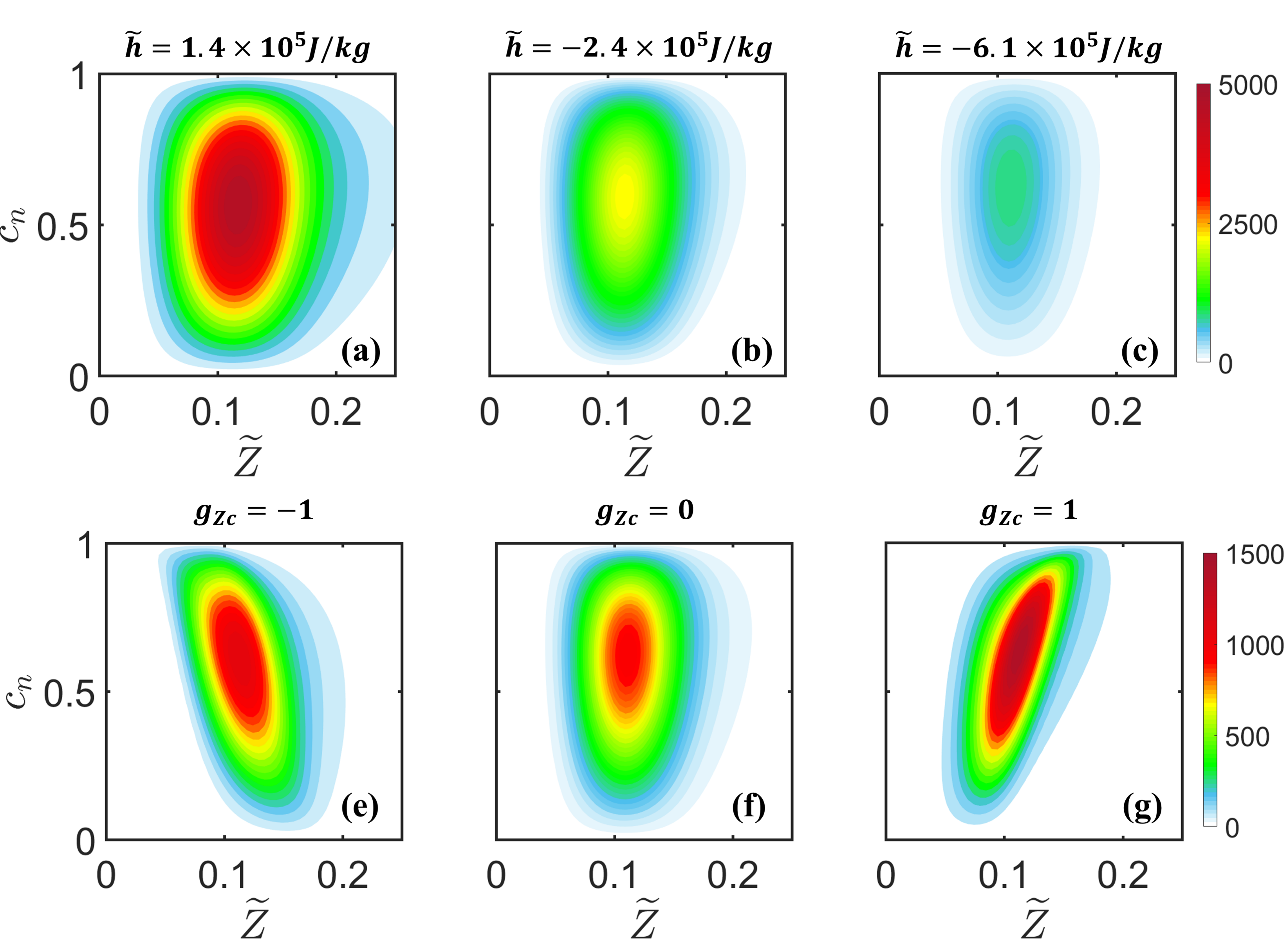
where $g_{Zc}=\widetilde{Z^{{}^{\prime\prime}}c^{{}^{\prime\prime}}}\big{/}\sqrt{\widetilde{Z^{{}^{\prime\prime}2}}\widetilde{c^{{}^{\prime\prime}2}}}$ is the correlation coefficient. Figure 1 presents the effect of introducing scalar correlation and evaporation heat loss effects via $g_{Zc}$ and $\widetilde{h}$ on filtered reaction rate as a function of $\widetilde{Z}$ and $c_{n}$. Intermediate value of $g_{Z}=0.0041$ and $g_{c}=0.4$ are used for illustration purpose, where $c_{n}=\widetilde{c}/\widetilde{c}_{max}$, $g_{Z}=\widetilde{Z^{{}^{\prime\prime}2}}\big{/}[\widetilde{Z}(1-\widetilde{Z})]$, $g_{c}=\widetilde{c^{{}^{\prime\prime}2}}\big{/}[\widetilde{c}(\widetilde{c}_{max}-\widetilde{c})]$. For mixtures with smaller total enthalpy, i.e. stronger evaporation heat loss, a drastic decrease in the reaction rate is observed as one would expect. As for the correlation effect, both positive and negative $g_{Zc}$ not only result in a positive or negative slope to the reaction rate contour, but also give increased maximum values of $\widetilde{\dot{\omega}_{c}}$. These findings generally align with the a priori analysis reported in [16].

2.3 Deep residual network

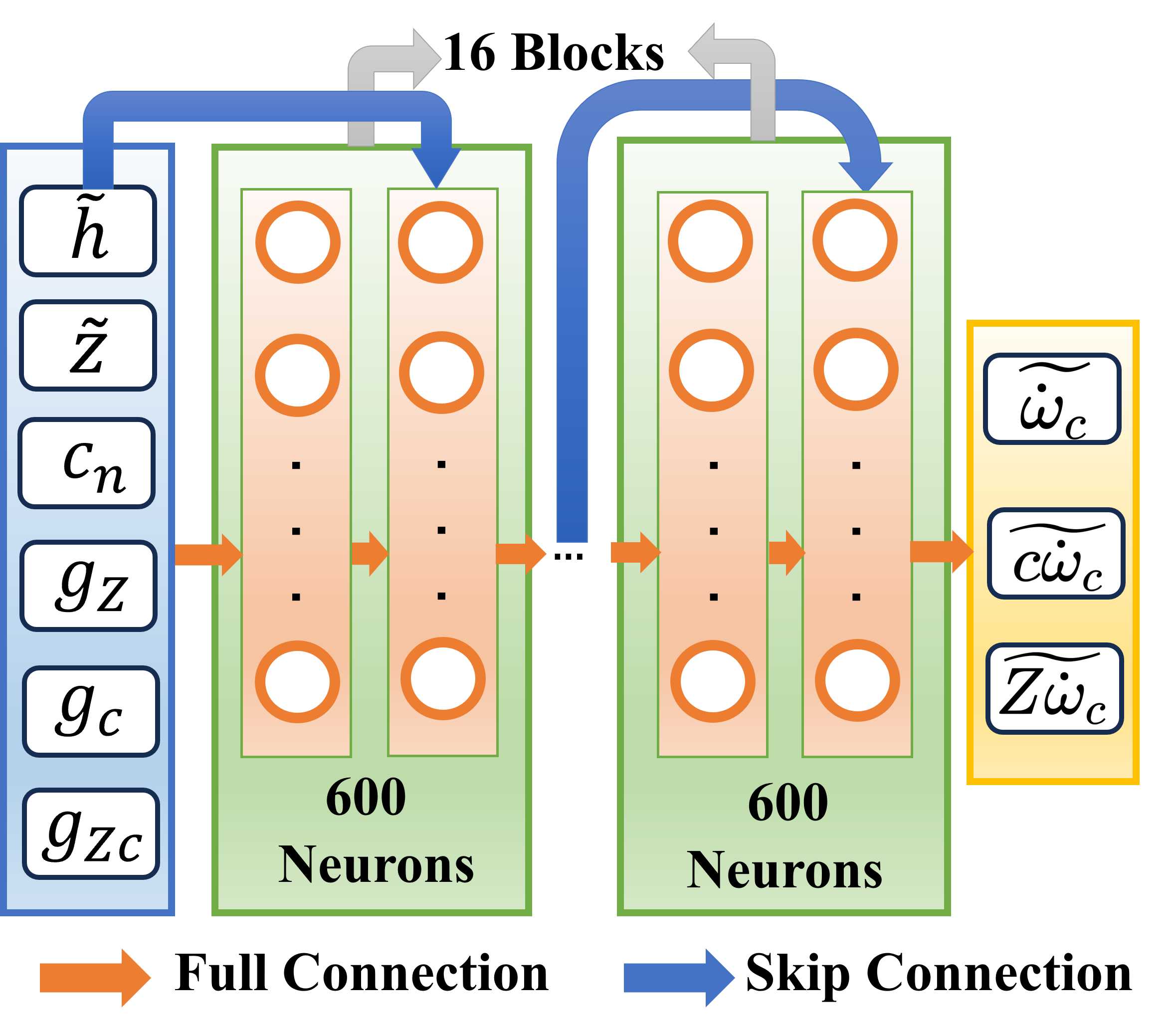
The deep residual network (ResNet) has been proven an effective tool in predicting the physical quantities in FGM lookup tables [20]. Figure 2 illustrates the structure of the ResNet model used to replace the 6-D table in this work. Variables in the blue box are the inputs, i.e. control parameters, while the yellow box marks the outputs for the three filtered reaction rates required to close the reactive scalar transport equations. The ResNet consists of 16 blocks and one block possesses one skip connection and two neural layers, each comprising 600 fully connected neurons.

Fig. 2: Architecture of the ResNet for 6-D table.

Fig. 3: Regression plot of the ResNet predicted reaction source terms: (a) $\widetilde{\dot{\omega}_{c}}$, (b) $\widetilde{c\dot{\omega}_{c}}$, and (c) $\widetilde{Z\dot{\omega}_{c}}$.

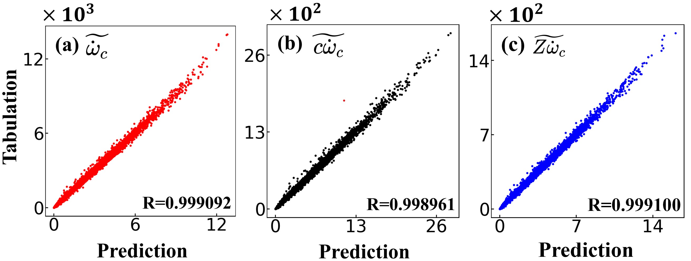
To process the 1 billion data points (12.1GB) in the 6-D chemical table, more layers and neurons are employed than those used in  [20]. Furthermore, due to the significant variations of the predicted variables, the Box-Cox transformation (BCT) [31] is applied to enhance the learning efficiency of the ResNet. The resulting size of the ResNet model is only 44MB, which is 1/300 of the original 6D table size. Figure 3 shows the regression of the predictive output of the ResNet. The mean square error (MES) is given by $R^{2}=1-\frac{\sum_{i=1}^{N}(y_{i}-\hat{y}_{i})^{2}}{\sum_{i=1}^{N}(y_{i}-\bar{y}_{i})^{2}}$. It is seen that all three reaction rates can be predicted well by the ResNet for a broad range of magnitudes with $R^{2}>0.998$.

3 Experiments and numerical details

The flame configuration experimentally studied at the University of Sydney [24, 25], is considered. Among those flames, the ethanol spray flame EtF4, showing high fluctuations in temperature [1], is simulated in this study. The spray burner consists of three streams, i.e., central jet, pilot, and air co-flow. The central jet, with a diameter $d_{jet}=$ 10.5mm, carries liquid and vapor fuel [25]. The pilot flow comprises a burnt stoichiometric mixture of acetylene/hydrogen and air, with a velocity of 11.6m/s [25]. The co-flow, with a velocity of 4.5m/s, is provided using a wind tunnel [24]. The detailed experimental conditions of EtF4 are provided in Table 1.

Table 1: Experimental conditions of the ethanol spray jet EtF4, experimental set A [24].

Parameter Value Bulk jet velocity (m/s) 24 Carrier (air) mass flow rate (g/min) 150 Liquid flow rate at jet exit (g/min) 14.5 Vapor fuel flow rate at jet exit (g/min) 8.9 Mixture fraction at jet exit 0.056 Jet Reynolds number 17,500

The simulations are performed using the dfSprayFoam solver of the open-source platform DeepFlame [32] developed based on OpenFOAM libraries. The computational domain extends to $35d_{jet}\times 10d_{jet}\times 2\pi$ in cylindrical coordinates, which is split to $450\times 123\times 56$ grid points in the axial, radial, and azimuthal directions, respectively. The SGS turbulence is approximated with the Smagorinsky model. The implicit Euler time-marching scheme is employed. Spatial gradients are evaluated via a second-order gradient scheme, while a second-order central difference scheme is adopted in the divergence terms. The inlet velocity of the central jet is given by the experimental data [24] at the cross-section $x/d_{jet}=0.3$, with a synthetic eddy turbulence generator [33] imposed. The injected droplet diameter is assigned with the Rosin-Rammler distribution, consistent with the measurements in experiments [24].

The non-adiabatic premixed flamelet table with $25\times 81\times 51\times 15\times 21\times 11$ grids in the $\widetilde{h}\times\widetilde{Z}\times c_{n}\times g_{Z}\times g_{c}\times g_{Zc}$ directions is computed using a skeletal ethanol mechanism with 31 species and 66 reactions [34]. An equidistant grid is employed in the $\widetilde{h}$ direction in the range of $-612516.1\sim 141483.9$ J/kg, where the minimum value corresponds to the lowest temperature in the mechanism and the maximum value corresponds to the maximum gas-phase temperature, 2493K. The grid in the $\widetilde{Z}$ direction is non-uniform in $[0,1]$, with refinement within the flammability limits. The grid along the $g_{Z}$ direction is logarithmically distributed within the range of $[0,0.1]$. The equidistant grids are utilized in the $c_{n}$ and $g_{c}$ direction over the interval $[0,1]$, as well as in the $g_{Zc}$ direction within the range of $[-1,1]$.

This work adopts the MPI shared memory technique based on the code provided in [18]. In order to manage the large volume of data, the table is assembled as $n_{pt}\times n_{var}$, which is different from [18], where $n_{var}$ is the number of physical quantities, $n_{pt}$ is the number of grid points per quantity. Thus, the procedure of table loading becomes ($i$) read the table to vector<vector<double>> temp, ($ii$) for each quantity, allocate shared memory to the master node using MPI_Win_allocate_shared, let slave nodes point to the address of shared memory using MPI_Win_shared_query, copy values from temp to shared memory, and free memory of the inner vector in temp using clear and swap. In this way, the memory footprint is limited to a maximum of $(1+1/n_{var})$ times the file size during the table loading process.

Fig. 4: Radial profile of mean gas temperature, $T$, and droplet axial mean velocity, $U_{p}$, compared with experiments.

4 Results and discussion

In this section, three different combustion tabulation methods are investigated: ($i$) the 6-D chemistry table, denoted as Tab6D; ($ii$) the 5-D table without the $g_{Zc}$ direction, denoted as Tab5D; ($iii$) the 6-D ResNet. Meanwhile, to examine the effect of $\widetilde{c}\overline{\dot{S}_{v}}$ in Eq. (3), Tab5D without $\widetilde{c}\overline{\dot{S}_{v}}$ is considered, denoted as No-Sv.

4.1 Instantaneous flow field

Fig. 5: Instantaneous snapshots at $t=0.21s$ of (a) the temperature, $T$, and (b) the density-weighted reaction rate, $\bar{\rho}\widetilde{\dot{\omega}_{c}}$. The combustion tabulation method is Tab6D.

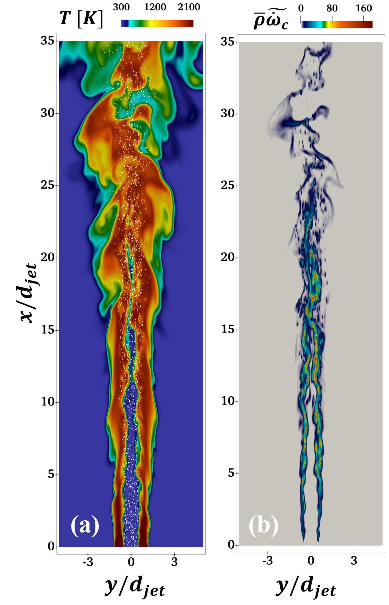
Figure 5 shows the snapshots of the temperature, $T$, and the density-weighted reaction rate, $\bar{\rho}\widetilde{\dot{\omega}_{c}}$, computed using Tab6D. Fuel droplet evaporates in the high-temperature region, participating in chemical reactions in the gaseous phase. At the jet exit plane, there is no chemical reaction rate in the blending zone of the fully burnt pilot flow and the air co-flow, as shown in Fig. 5b. This is the reason why the unscaled $\widetilde{c}$ is chosen, instead of the scaled one in [2]. Truncating $\widetilde{\dot{\omega}_{c}}$ according to fuel mass fraction is not suitable, since the extinction of ethanol, as a macro-molecular species, cannot signify the completion of the chemical reaction. In such area, the transport equation of $Y_{c}$ is conservative, thus $\widetilde{\dot{\omega}_{c}}=0$ is naturally obtained.

4.2 Comparision with measurements

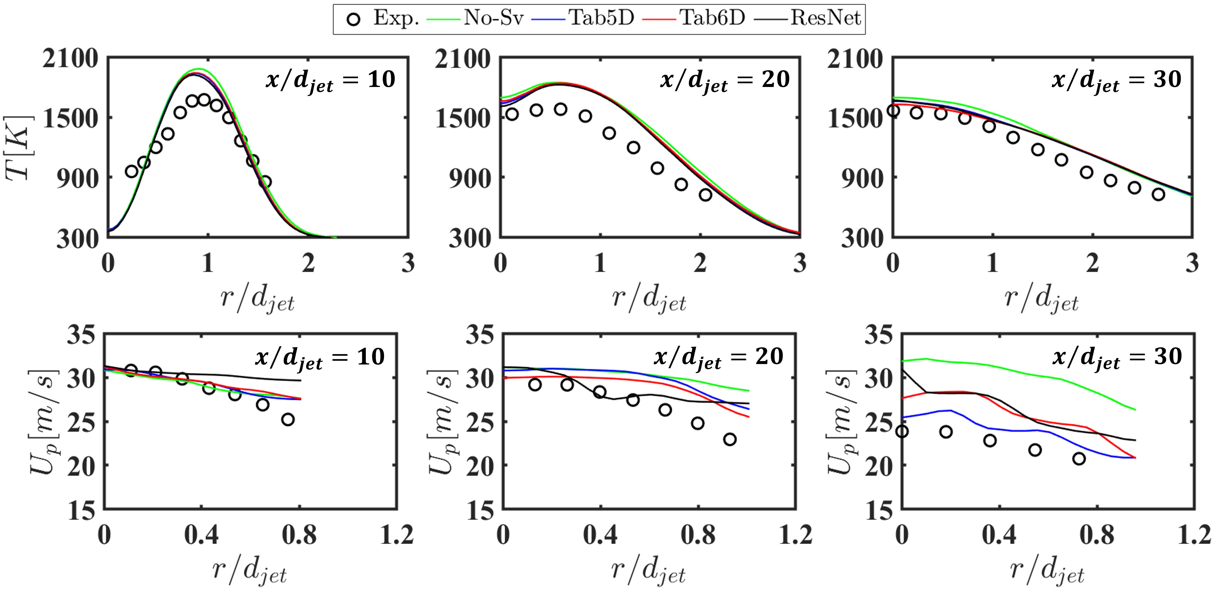
Figure 4 presents the comparison of radial profiles of the mean gas-phase temperature $T$ and mean liquid-phase axial velocity $U_{p}$ with experimental data. Generally, the simulated temperatures are in good agreement with the measurements. The flame spreading is well predicted at axial planes $x/d_{jet}=10$ and $x/d_{jet}=20$. Compared to Tab5D, simulation with the covariance can better predict the temperature in the reacting zone downstream. Effects of the correlation coefficient on the reaction rates accelerate the progress of the chemical reaction along the axis of the computation domain, resulting in a higher temperature at $x/d_{jet}=20$ and a lower temperature at $x/d_{jet}=30$ than in Tab5D. The temperature field calculated through ResNet exhibits a notable consistency with those obtained from tabulation. The calculation without the source term $\widetilde{c}\overline{\dot{S}_{v}}$ in Eq. (3) results in the poorest performance in capturing the heat loss effect due to evaporation.

At the upstream locations, the radial profiles of droplet mean axial velocity are in good agreement with measurements, while at the downstream location, a visible discrepancy is noticed. This is attributed to the higher computed temperature [2]. In the regions of elevated temperature at $x/d_{jet}=20$, small droplets experience significant evaporation, while large droplets with low speed can persist, resulting in a flat radial profile of mean axial velocity. At the downstream plane, the droplet axial velocity in No-Sv is much higher than in other simulations.

Fig. 6: Instantaneous scatter plot of $\widetilde{\dot{\omega}_{c}}$ over mass fraction.

4.3 Effect of heat loss

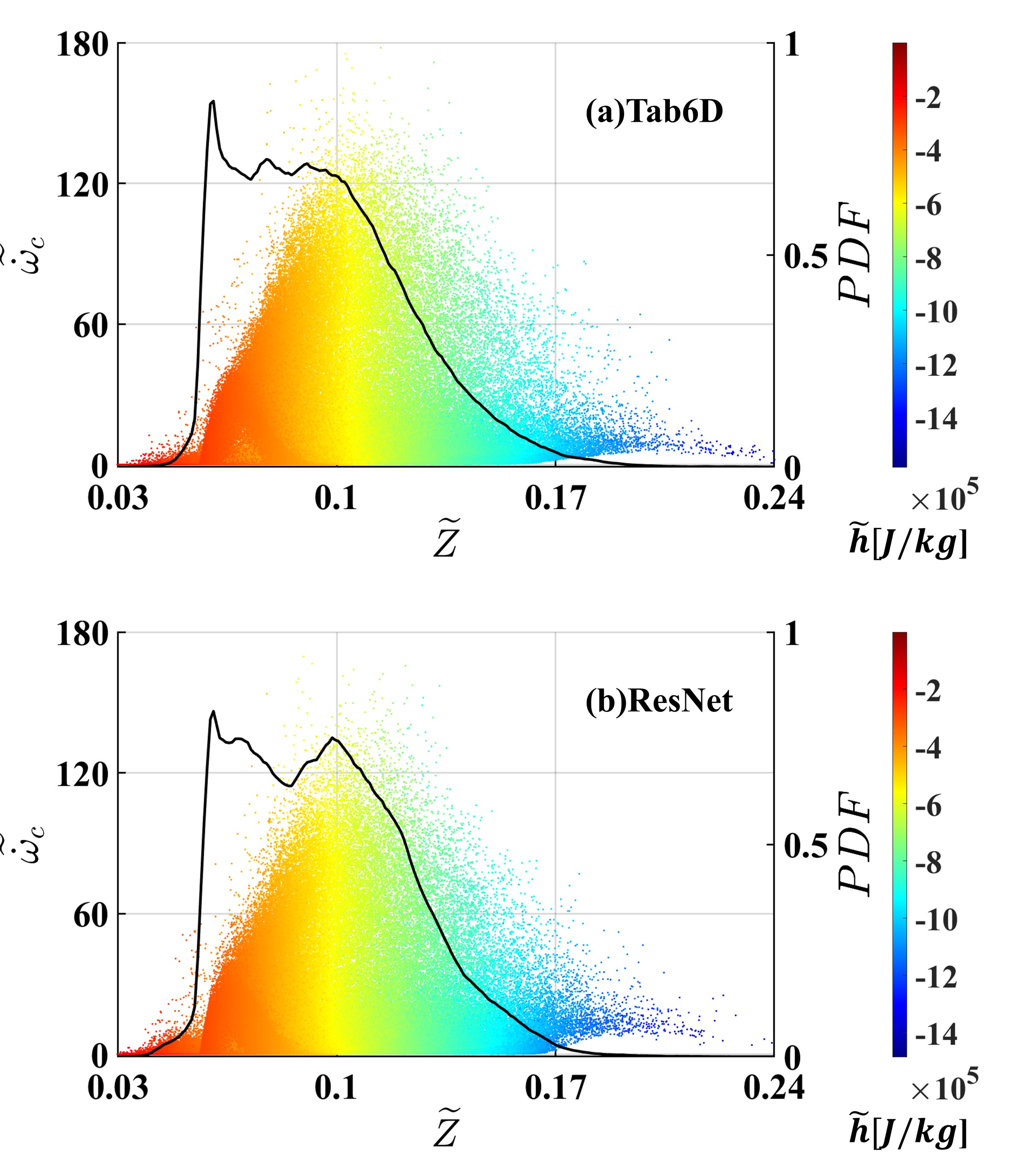
Fig. 6 presents the instantaneous scatter of the reaction rate $\widetilde{\dot{\omega}_{c}}$, colored by enthalpy $\widetilde{h}$ over the mass fraction $\widetilde{Z}$. The PDF of reacting points ($\widetilde{\dot{\omega}_{c}}>1$) represented by the black line is also superimposed. Due to particle evaporation, there is an enthalpy loss in the corresponding gas phase, accompanied by an increase in mixture fraction. The PDF distribution illustrates that half of the chemical reactions are lean combustion ($\widetilde{Z}<0.1$), while some rich combustion occurs following the evaporation of droplets. Comparison between Fig. 6(a) and Fig. 6(b) illustrates that ResNet shares a similar sampling space in $\widetilde{h}\times\widetilde{Z}$ directions as Tab6D, while the PDF distribution at $\widetilde{Z}=0.1$ is slightly different.

4.4 Interaction between droplet evaporation and covariance $\widetilde{Z^{{}^{\prime\prime}}c^{{}^{\prime\prime}}}$

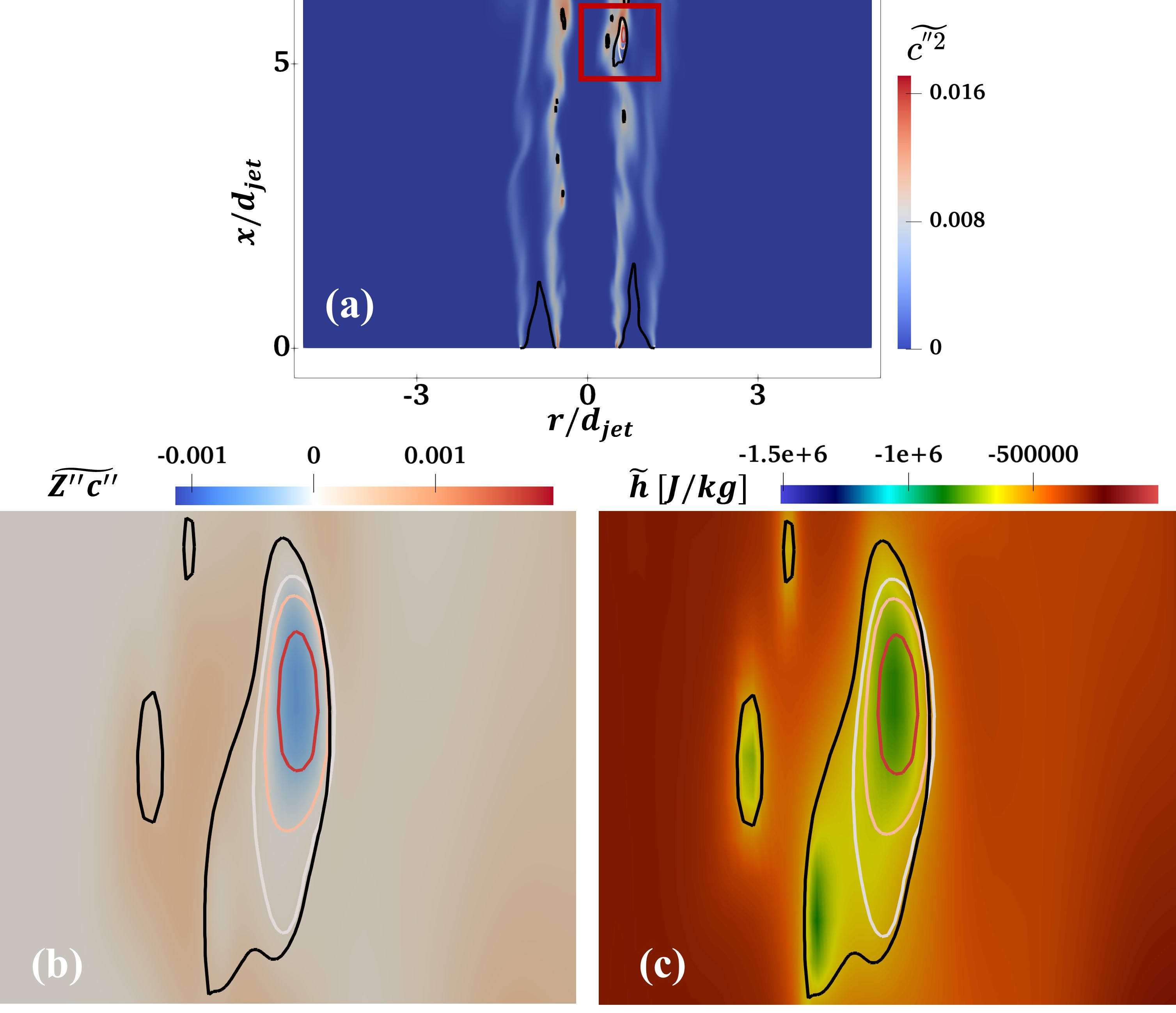
Fig. 7 shows the instance $\widetilde{c^{{}^{\prime\prime}2}}$, $\widetilde{Z^{{}^{\prime\prime}}c^{{}^{\prime\prime}}}$ and $\widetilde{h}$ fields, at the same time as in Fig. 5. The flow area chosen for illustration is a reacting zone with non-zero $\widetilde{c^{{}^{\prime\prime}2}}$ at $x/d_{jet}=5$, $y/d_{jet}=0.5$. The black contour denotes the stoichiometric mixture fraction, $\widetilde{Z_{st}}$. With droplet evaporation, $\widetilde{h}$ decreases, and $\widetilde{Z}$ increases. Variation of $\widetilde{Z}$ induces a greater $\widetilde{Z^{{}^{\prime\prime}2}}$ in SGS, while $\widetilde{c^{{}^{\prime\prime}2}}$ is reduced due to dissipation effect. As a result, $\widetilde{Z^{{}^{\prime\prime}}c^{{}^{\prime\prime}}}$ becomes negative. All those combustion scalars can alter the temperature via table look-up and ideal gas state equation. The gas-phase temperature can directly influence the droplet evaporation rate.

Fig. 7: Instantaneous snapshot of (a) $\widetilde{c^{{}^{\prime\prime}}}$, (b) $\widetilde{Z^{{}^{\prime\prime}}c^{{}^{\prime\prime}}}$, and (c) $\widetilde{h}$. The location of (b) and (c) is marked out with a red box in (a). Contours are plotted as: $\widetilde{Z}=\widetilde{Z_{st}}=0.1$ (black), $\widetilde{Z^{{}^{\prime\prime}2}}=5e^{-4}$ (white), $\widetilde{Z^{{}^{\prime\prime}2}}=6e^{-4}$ (orange), and $\widetilde{Z^{{}^{\prime\prime}2}}=8e^{-4}$ (red).

5 Conclusion

This study introduced a comprehensive joint PDF method for the $posteriori$ examination of the subgrid correlation involving mixture fraction and progress variable within the framework of LES and flamelet modeling. Utilizing a residual network and the MPI shared memory technique, high-dimensional tabulations were realized. Those methodologies were applied in the LES simulation of the ethanol spray flame EtF4 [24, 25]. The simulations employing different combustion tabulation methods exhibited good agreement with experiments.

The impact of the correlation coefficient on the chemical reaction rate was two-fold: ($i$) an increase in the peak value and ($ii$) an alteration in the slope of the reaction rate concerning mass fraction and progress variable. In the ResNet model, a satisfactory prediction performance of tabulated physical quantities was achieved. Memory consumption was significantly reduced from 12.1GB in the chemical table to 44MB in the ResNet. The simulation results using ResNet exhibited a notable consistency with those obtained with the chemical table. The influence of heat loss was considered in these tabulations. Numerous chemical reactions occurred in regions associated with enthalpy losses due to evaporation.

The interaction between droplet evaporation and covariance was elucidated and discussed. The vaporized fuel resulted in a decrease in $\widetilde{h}$ and an increase in $\widetilde{Z}$ and $\widetilde{Z^{{}^{\prime\prime}2}}$, leading to a positive or negative $\widetilde{Z^{{}^{\prime\prime}}c^{{}^{\prime\prime}}}$ if $\widetilde{c^{{}^{\prime\prime}2}}\neq 0$. These scalars, in turn, affected the evaporation rate with temperature variation. Due to the evaporation effect, the source term $\widetilde{c}\overline{\dot{S}_{v}}$ was introduced in the transport equation of progress variable, i.e., Eq. (3). Compared with the simulation without $\widetilde{c}\overline{\dot{S}_{v}}$, Eq. (3) can better capture the gas temperature distribution. Moreover, the unscaled progress variable was shown to well describe the reaction rate in the blending zone of the fully burnt pilot flow and the air co-flow at the location close to the jet exit.

Declaration of competing interest

The authors declare that they have no known competing financial interests or personal relationships that could have appeared to influence the work reported in this paper.

Acknowledgments

This work is supported by the National Natural Science Foundation of China (Grant Nos. 92270203 and 52276096).

References

- [1] S. De, S. H. Kim, Large eddy simulation of dilute reacting sprays: Droplet evaporation and scalar mixing, Combust. Flame 160 (10) (2013) 2048–2066.
- [2] Y. Hu, R. Kurose, Partially premixed flamelet in LES of acetone spray flames, Proc. Combust. Inst. 37 (3) (2019) 3327–3334.
- [3] N. J. Georgiadis, D. P. Rizzetta, C. Fureby, Large-Eddy Simulation: Current Capabilities, Recommended Practices, and Future Research, AIAA J. 48 (8) (2010) 1772–1784.
- [4] X. Jiang, G. A. Siamas, K. Jagus, T. G. Karayiannis, Physical modelling and advanced simulations of gas-liquid two-phase jet flows in atomization and sprays, Prog. Energ. Combust. 36 (2) (2010) 131–167.
- [5] E. Quadarella, A. Péquin, A. Stagni, A. Parente, T. Faravelli, H. G. Im, A generalized partially stirred reactor model for turbulent closure, Proc. Combust. Inst. 39 (4) (2023) 5329–5338.
- [6] M. J. Evans, C. Petre, P. R. Medwell, A. Parente, Generalisation of the eddy-dissipation concept for jet flames with low turbulence and low Damköhler number, Proc. Combust. Inst. 37 (4) (2019) 4497–4505.
- [7] S. Ukai, A. Kronenburg, O. T. Stein, LES-CMC of a dilute acetone spray flame, Proc. Combust. Inst. 34 (1) (2013) 1643–1650.
- [8] L. Xu, Y. Zhang, Q. Tang, B. Johansson, M. Yao, X. Bai, LES/FGM investigation of ignition and flame structure in a gasoline partially premixed combustion engine, Proc. Combust. Inst. 39 (4) (2023) 4851–4860.
- [9] C. D. Pierce, Progress-variable approach for large-eddy simulation of turbulent combustion, Ph.D. thesis, Stanford University (2001).
- [10] P. Wollny, B. Rogg, A. Kempf, Modelling heat loss effects in high temperature oxy-fuel flames with an efficient and robust non-premixed flamelet approach, Fuel 216 (2018) 44–52.
- [11] T. Tang, H. B. Wang, M. B. Sun, G. Y. Zhao, J. F. Yu, Z. Q. Fan, Z. G. Wang, Evaluation of flamelet/progress variable model for the applications in supersonic combustion using hybrid RANS/LES approach, Aerosp. Sci. Technol. 126 (2022) 107633.
- [12] M. Ihme, H. Pitsch, LES of a non-premixed flame using an extended flamelet/progress variable model, in: 43rd AIAA Aerospace Sciences Meeting and Exhibit, 2005, p. 558.
- [13] R. S. Barlow, G. Magnotti, H. C. Cutcher, A. R. Masri, On defining progress variable for Raman/Rayleigh experiments in partially-premixed methane flames, Combust. Flame 179 (2017) 117–129.
- [14] V. Robin, A. Mura, M. Champion, O. Degardin, B. Renou, M. A. Boukhalfa, Experimental and numerical analysis of stratified turbulent V-shaped flames, Combust. Flame 153 (2008) 288–315.
- [15] V. Jaganath, M. Stoellinger, Transported and presumed probability density function modeling of the sandia flames with flamelet generated manifold chemistry, Physics of Fluids 33 (4) (2021) 045123.
- [16] Z. X. Chen, N. A. K. Doan, S. Ruan, I. Langella, N. Swaminathan, A priori investigation of subgrid correlation of mixture fraction and progress variable in partially premixed flames, Combust. Theor. Model. 22 (5) (2018) 862–882.
- [17] Z. Nikolaou, L. Vervisch, P. Domingo, Criteria to switch from tabulation to neural networks in computational combustion, Combust. Flame 246 (2022) 112425.
- [18] Y. Zhang, Combustion model development based on flamelet generated manifolds and application on partially premixed combustion, Ph.D. thesis, Tianjin University (2021).
- [19] T. Hoefler, J. Dinan, D. Buntinas, P. Balaji, B. Barrett, R. Brightwell, W. Gropp, V. Kale, R. Thakur, MPI + MPI: a new hybrid approach to parallel programming with MPI plus shared memory, Combust. Flame 95 (2013) 1121––1136.
- [20] M. Hansinger, Y. Ge, M. Pfitzner, Deep Residual Networks for Flamelet/progress Variable Tabulation with Application to a Piloted Flame with Inhomogeneous Inlet, Combust. Sci. Technol. 194 (8) (2022) 1587–1613.
- [21] I. Matthias, A. L. Marsden, H. Pitsch, Generation of Optimal Artificial Neural Networks Using a Pattern Search Algorithm: Application to Approximation of Chemical Systems, Neural Comput. 20 (2) (2008) 573–601.
- [22] Y. Zhang, S. Xu, S. Zhong, X. Bai, H. Wang, M. Yao, Large eddy simulation of spray combustion using flamelet generated manifolds combined with artificial neural networks, Energy AI 2 (2020) 100021.
- [23] R. B. Nelsen, An introduction to copulas, Springer, New York, 2006.
- [24] J. D. Gounder, A. Kourmatzis, A. R. Masri, Turbulent piloted dilute spray flames: Flow fields and droplet dynamics, Combust. Flame 159 (11) (2012) 3372–3397.
- [25] J. D. Gounder, An experimental investigation of non-reacting and reacting spray jets, Ph.D. thesis, University of Sydney (2009).
- [26] Y. Hu, R. Kurose, Nonpremixed and premixed flamelets LES of partially premixed spray flames using a two-phase transport equation of progress variable, Combust. Flame 188 (2018) 227–242.
- [27] Z. X. Chen, Simulation of Partially Premixed Turbulent Flames, Ph.D. thesis, University of Cambridge (2016).
- [28] N. S. S. Ruan, O. Darbyshire, Modelling of turbulent lifted jet flames using flamelets: a priori assessment and a posteriori validation, Combust. Theor. Model. 18 (2) (2014) 295–329.
- [29] O. R. Darbyshire, N. Swaminathan, A Presumed Joint pdf Model for Turbulent Combustion with Varying Equivalence Ratio, Combust. Sci. Technol. 184 (12) (2012) 2036–2067.
- [30] P. P. Popov, Alternatives to the Beta Distribution in Assumed PDF Methods for Turbulent Reactive Flow, Flow Turbulence Combust. 108 (2022) 433––459.
- [31] G. E. Box, D. R. Cox, An analysis of transformations, Journal of the Royal Statistical Society Series B: Statistical Methodology 26 (2) (1964) 211–243.
- [32] R. Mao, M. Lin, Y. Zhang, T. Zhang, Z. J. Xu, Z. X. Chen, DeepFlame: A deep learning empowered open-source platform for reacting flow simulations, Comput. Phys. Commun. 291 (2023) 108842.
- [33] N. Kornev, E. Hassel, Method of random spots for generation of synthetic inhomogeneous turbulent fields with prescribed autocorrelation functions, Commun. Numer. Meth. En. 23 (1) (2007) 35–43.
- [34] A. Millán-Merino, E. Fernández-Tarrazo, M. Sánchez-Sanz, F. A. Williams, A multipurpose reduced mechanism for ethanol combustion, Combust. Flame 193 (2018) 112–122.