Boosting Transformer’s Robustness in PPG Signals Artifact Detection with Self-Supervised Learning

Abstract

Recent research at CHU Sainte-Justine’s Pediatric Critical Care Unit (PICU) has revealed that traditional machine learning methods, such as semi-supervised label propagation and K-nearest neighbors, outperform Transformer-based models in artifact detection from PPG signals, mainly when data is limited. This study addresses the underutilization of abundant unlabeled data by employing self-supervised learning (SSL) to extract latent features from these data, followed by fine-tuning on labeled data. Our experiments demonstrate that SSL significantly enhances the Transformer model’s ability to learn representations, thereby improving its robustness in artifact classification tasks. Among various SSL techniques—including masking, contrastive learning, and DINO (self-distillation with no labels)—contrastive learning exhibited the most stable and superior performance in small PPG datasets. Further, we delve into optimizing contrastive loss functions, which are crucial for contrastive SSL. Inspired by InfoNCE, we introduce a novel contrastive loss function that facilitates smoother training and better convergence, thereby enhancing performance in artifact classification. In summary, this study establishes the efficacy of SSL in leveraging unlabeled data, particularly in enhancing the capabilities of the Transformer model. This approach holds promise for broader applications in PICU environments, where annotated data is often limited.

I Introduction

Recently, the Pediatric Intensive Care Unit (PICU) at CHU Sainte-Justine (CHUSJ) has made notable advancements by developing a high-resolution research database (HRDB) [1, 2]. This innovative database directly integrates biomedical signals from various monitoring devices into the electronic patient record, ensuring seamless data incorporation throughout a patient’s PICU stay [3]. The integration of HRDB has significantly enhanced the Clinical Decision Support System (CDSS) at CHUSJ, boosting patient safety and underpinning decision-making with robust evidence [4]. In this context, early and accurate diagnosis of acute respiratory distress syndrome (ARDS) is a pivotal goal of the CDSS at CHUSJ. Oxygen saturation (SpO2) values, critical in ARDS diagnosis, are central to predicting and managing ARDS [5, 6], and play a key role in determining respiratory support strategies [7, 8, 9]. Moreover, the potential to predict SpO2 from Photoplethysmography (PPG) waveforms and non-invasive blood pressure estimation is increasingly recognized for its integral role in enhancing CDSS capabilities [10, 11]. Consequently, accurately identifying and removing erroneous waveforms and SpO2 values from CDSS inputs is crucial. Ensuring the reliability of these inputs is essential for the effective functioning of the CDSS, directly impacting patient outcomes and care efficiency. Building on the foundation of our work in fully-supervised and semi-supervised learning methodologies, we have delved into the domain of PPG artifact detection, focusing on machine learning (ML) applications. A pivotal study in this area [12] investigated the use of machine learning techniques for this purpose. However, challenges arise in scenarios featuring imbalanced classes and limited data availability. In these contexts, Transformer models, despite their advanced attention mechanisms, have exhibited suboptimal performance compared to other methods, such as semi-supervised label propagation and supervised KNN learning. The core issue lies in the Transformer models’ reduced efficacy in smaller datasets. To address these limitations and enhance the Transformer’s applicability in artifact detection, our recent study [13] introduced an innovative approach. We incorporated the Gated Residual Network (GRN) into the Transformer framework, enhancing its performance capabilities significantly. This GRN-Transformer hybrid model not only overcomes the inherent limitations of traditional Transformer models in handling smaller datasets but also outperforms other existing models in artifact detection accuracy and reliability. Despite these advancements in artifact detection, a common limitation persists across recent studies: a heavy reliance on annotated data to train fully supervised machine learning algorithms. This reliance is particularly evident considering that in most cases, only up to 10% of the data is annotated, leaving a vast 90% of the data pool unexploited. Such underutilization of available data presents a significant challenge, especially when dealing with small datasets and imbalanced classes, which are common in the task of binary classification for motion artifact detection in PPG signals. In light of these challenges, this study aims to transcend the constraints of labeled data dependency by harnessing the potential of SSL. This approach is particularly pertinent for two key reasons as follows: i) The vast majority of our data, approximately 90%, remain unannotated, representing a largely untapped resource that could significantly enhance our understanding and detection capabilities, and ii) There is a compelling opportunity to explore how SSL can adapt and perform with limited and unlabeled data, a scenario frequently encountered in clinical settings. By pivoting towards SSL, we aim to leverage the underused unannotated data, potentially revolutionizing how we approach artifact detection and enhancing the robustness of our classification models in these challenging PICU environments.

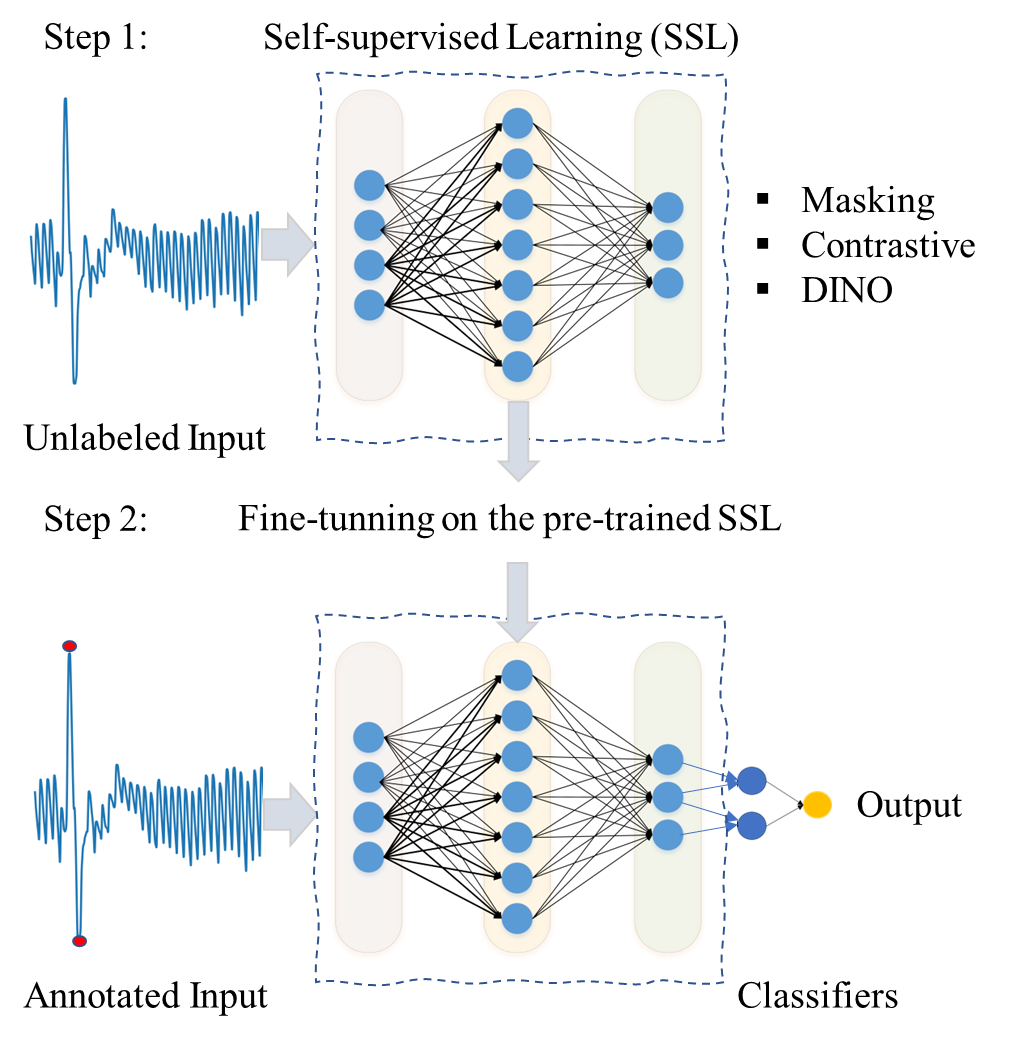
Figure 1: An end-end process diagram workflow demonstration.

In our quest to validate the efficacy of SSL in PPG artifact classification, as shown in Fig. 1, we explored three distinct SSL mechanisms: masking, contrastive learning, and self-distillation without labels (DINO). Masking involves intentionally obscuring parts of the input data, prompting the model to predict these missing parts, thereby learning robust data representations. Contrastive learning focuses on learning by comparing similar and dissimilar pairs of data points, enhancing the model’s ability to discern subtle differences and similarities within the data. DINO, or self-distillation without labels, leverages a teacher-student network architecture where the ‘student’ model learns to mimic the output of a ‘teacher’ model, which is typically more powerful or pre-trained, even without labeled data. In the workflow Fig. 1, the model first (Step 1) undergoes pre-training with techniques like masking, contrastive learning, and DINO on unannotated data, allowing it to capture intrinsic PPG signal patterns. Following this, the pre-trained model is fine-tuned on a labeled dataset (Step 2), focusing on its ability to accurately classify and detect artifacts. This two-tiered approach leverages the extensive unannotated data for foundational learning and a smaller annotated dataset for precision, equipping the model with robust generalization capabilities for effective artifact detection. Consequently, the experimental results underscored a significant finding: employing these SSL techniques to initially train on unlabeled data, followed by fine-tuning on a smaller proportion (10%) of labeled data, markedly improved the classification performance over models trained exclusively on fully-supervised learning with limited labeled data. Specifically, the Transformer model is robust and effective compared to other backbone neural networks when it is elaborated with SSL. Second, contrastive learning emerged as the most effective among the three SSL techniques tested. However, its success is heavily contingent upon the design of the contrastive loss functions. Therefore, we delved further into investigating various contrastive losses. A notable improvement was the adaptation and enhancement of the InfoNCE loss function, which proved to be particularly effective in augmenting the performance of contrastive models. Lastly, unsupervised learning also helps the Transformer’s performance; however, it can not beat SSL’s efficacy in all data proportion cases.

II Related Works

The accuracy and reliability of pulse oximeters, essential for monitoring blood oxygen levels, are significantly impacted by motion artifacts in PPG signals [14]. Traditional filtering algorithms, while helpful, are not fully effective in eliminating these motion artifacts. As a result, residual motion artifacts often lead to inaccuracies in the measurement of blood oxygen saturation. This underscores the importance of developing more sophisticated methods for detecting and mitigating motion artifacts in PPG signals to ensure the reliability and precision of pulse oximetry readings. In the PICU setting, the necessity for accurate PPG artifact detection becomes even more pronounced [12]. Children, especially those in critical care, are often prone to more frequent and abrupt movements compared to adults. Therefore, enhancing PPG signal processing to accurately identify and compensate for these artifacts is vital for improving patient monitoring and care quality in pediatric intensive care settings.

The integration of ML into PPG analysis has revolutionized a range of clinical applications, addressing diverse healthcare needs with greater precision. A notable example is heart rate estimation, where ML models have shown exceptional accuracy, as highlighted in the studies by Dao et al. [15] and Mehrgardt et al. [16]. This advancement extends beyond basic applications; ML also enables real-time physiological monitoring. It provides critical insights into vital signs such as blood pressure [17], oxygen saturation [11], and respiratory rate [18], thereby enhancing patient care and enabling the early identification of potential health issues, as shown in research by Venema et al. [19] and Alharbi et al. [20]. Furthermore, ML algorithms have been particularly effective in the detection and filtration of motion artifacts in PPG data, a crucial step in ensuring the reliability of continuous monitoring systems, as demonstrated by Nwibor et al. [21]. In summary, the application of ML in PPG analysis has not only broadened the scope of clinical applications but has also significantly increased the efficiency and accuracy of healthcare interventions.

The implementation of conventional ML techniques marked initial advancements in this field. For instance, Support Vector Machine classifiers have demonstrated efficacy in detecting heart rates from PPG signals, employing time-frequency spectral features [15]. This approach represents the foundational phase of machine learning applications in PPG analysis. However, the field has witnessed a significant shift towards more sophisticated methods, particularly with the advent of deep learning algorithms. Studies have increasingly adopted deep learning models like Multilayer Perceptrons and Fully Convolutional Neural Networks, which have shown promising results in artifact detection [22, 23]. These advancements reflect a transition from conventional machine learning techniques to more complex and capable deep learning methods within the supervised learning paradigm, significantly enhancing the capabilities in PPG signal analysis.

Recent advancements in PPG signal analysis underscore a paradigm shift from traditional supervised learning methods to exploring the potential of unsupervised and semi-supervised approaches. Initial studies, such as the one by Maqsood et al. [24], have demonstrated the effectiveness of deep learning algorithms, particularly Bi-LSTM combined with time-domain features, in achieving superior heart rate estimation. This approach primarily relied on supervised learning frameworks. However, our research team’s study [12] marks a significant transition in this domain. We explored a range of ML techniques, encompassing not only conventional machine learning and supervised models like MLP and Transformer but also semi-supervised learning with label propagation. Interestingly, we found that semi-supervised label propagation and the supervised KNN algorithm exhibited better performance than Transformer models, especially in scenarios involving imbalanced classes and limited data. This finding indicates a growing trend toward leveraging semi-supervised methods in PPG artifact detection, highlighting their potential to overcome data scarcity and class imbalance challenges.

In light of the demonstrated advantages of SSL, this study will focus primarily on this approach, particularly its effectiveness in providing robust representations for downstream tasks without the need for labeled data. SSL can significantly enhance robustness in various aspects, including resistance to adversarial examples, resilience against label corruption, and tolerance to common input corruption. Moreover, an intriguing aspect of self-supervision is its remarkable capability to aid out-of-distribution detection, especially with challenging near-distribution outliers. In fact, in these scenarios, self-supervision has been observed to surpass the performance of fully supervised methods, as detailed in the study by Hendrycks et al. [25]. These insights demonstrate the potential of self-supervision in improving robustness and uncertainty estimation and establish these domains as critical avenues for future research in SSL. Our study, therefore, seeks to delve deeper into these promising aspects of self-supervision, aiming to contribute meaningful advancements in artifact detection.

In conclusion, the integration of ML in PPG analysis has marked a significant milestone in the field, especially in enhancing artifact detection. This advancement has improved signal reliability and opened new frontiers in clinical applications. However, this domain still requires extensive research and development to fine-tune these methodologies and ensure their effective integration into clinical practices. This ongoing progression is set to redefine the landscape of PPG signal analysis and its consequential impact on patient care, particularly in the PICU at CHUSJ. Additionally, despite the transformative potential of Transformer models and attention mechanisms in ML, as surveyed by Lin et al. [26], their efficacy in small dataset scenarios remains a challenge, as highlighted in studies by our studies [12, 16, 27]. This study, therefore, was driven by the objective of augmenting the SSL capability in effectively managing small datasets and imbalanced classes. Our focus is particularly on the classification task of detecting motion artifacts in PPG signals, a critical aspect of ensuring accurate and reliable patient monitoring.

III Materials and Methods

III-A Clinical PPG Data at CHUSJ

The PICU at CHUSJ has implemented a high-resolution research database (HRDB), which has received approval from the ethical committee. This HRDB is a comprehensive system that effectively integrates biomedical signals from various monitoring devices with electronic patient records. This integration occurs throughout each patient’s hospital stay, providing a rich and detailed dataset for research purposes.

The research protocol conducted for this study received approval from the research ethics board of CHUSJ, University of Montreal under the project number eNIMP:2023-4556. The data collection process within this HRDB captures a wide range of physiological signals. Key among these was the pulse oximeter sensor, which played a crucial role in acquiring PPG signals. This sensor works by emitting light into the skin and measuring the variations in light absorption due to blood flow changes during the cardiac cycle. Additionally, blood pressure signals were recorded through non-invasive methods, offering a comprehensive view of blood pressure dynamics.

The study’s population included children aged from newborn to 18 years who were admitted to CHUSJ between September 2018 and September 2023. The inclusion criteria were based on the availability of essential waveform records such as ECG, PPG, and ABP. Certain exclusion criteria were applied to maintain the integrity and quality of the data. Any data collected after the fourth day of hospitalization were excluded to minimize potential biases. Moreover, the study did not include patients undergoing Extracorporeal Membrane Oxygenation (ECMO) treatment. In cases of multiple readmissions, only data from the initial admission were considered to maintain data independence and avoid confounding factors.

The final cohort comprised 1,573 eligible patients. For each patient, continuous recordings of ECG, PPG, blood pressure via catheter, and cuff blood pressure were made over a 96-hour period. The PPG signals were specifically captured every 5 seconds at a sampling frequency of 128 Hz. Similarly, blood pressure and ECG signals were acquired with a frequency of 512 Hz, also at 5-second intervals. During the data extraction phase, a fixed 30-second window was employed for each PPG signal to facilitate subsequent processing and analysis.

III-B Data Pre-Processing

In our study, data preprocessing plays a crucial role in enhancing the quality of PPG signals and involves four key steps. This process encompasses four main steps: filtering, segmentation, resampling and normalization, and feature extraction. Initially, each signal is refined using a bandpass Butterworth filter with frequencies between 0.5 Hz and 5 Hz, effectively removing baseline wander and high-frequency noise. Subsequently, the signal is segmented into smaller pulses by identifying local minima, enabling precise artifact detection within each pulse. Each pulse is then uniformly resampled to 256 samples, corresponding to a one-second heart cycle, and normalized to ensure a consistent feature scale. Finally, feature extraction focuses on the signal’s temporal characteristics, with samples taken every four milliseconds to capture the complete temporal profile of each pulse. These preprocessing steps are critical for ensuring data quality and reliability for subsequent analysis.

A manual annotation process is employed to establish ground truth for classification assessment. An expert annotates each PPG signal pulse based on its morphology and characteristics. Additionally, a secondary algorithm, acting as a supplementary expert, reannotates all pulses and employs statistical analysis to determine normative pulse values. The comparison of annotations from both the expert and the algorithm enhances the accuracy and reliability of artifact detection, thereby ensuring robust analysis.

In our final phase of refining the machine learning algorithms for automated artifact classification, we conducted experiments with different proportions of the dataset being annotated. This approach aimed to identify the minimum dataset size necessary for effective annotation. We methodically annotated subsets of 2.5%, 5%, 7.5%, and 10% of the entire dataset, examining each to ascertain the most efficient subset size for optimal performance in artifact detection.

III-C Self-Supervised Learning (SSL)

SSL represents a breakthrough in machine learning, offering an innovative way for systems to understand and process data. Unlike traditional supervised learning that depends on human-provided labeled data, SSL generates training signals from the unlabeled data. It formulates a proxy objective, often by creating tasks where the model predicts part of the data from other parts. SSL avoids trivial solutions by employing strategies such as contrastive methods, like SimCLR and its InfoNCE criterion, which distinguish between positive and negative examples, or non-contrastive methods that apply regularization to prevent model collapse. The key advantages of SSL include its efficiency in reducing the need for extensive manual labeling, its ability to learn rich data representations beneficial for various downstream tasks, and its flexibility to be applied to diverse data types. This approach has been gaining traction, especially in fields like computer vision and natural language processing, due to its effective utilization of large volumes of unlabeled data [28].

Among SSL approaches, three notable techniques stand out, each offering unique approaches to training models on unlabeled data. Each of these techniques embodies the essence of SSL by extracting valuable information from unlabeled data, thereby broadening the scope and efficiency of machine learning models in various domains.

III-C1 Masking

The masking approach for SSL, as depicted in the pseudo Algorithm 1, is a technique that involves selectively hiding parts of the input data and then training a model to predict these masked portions. This approach is widely used in various domains, such as natural language processing (e.g., BERT [29]) and computer vision, to learn robust data representations without the need for labeled data. An explanation of the provided pseudo-algorithm is as follows: i) First, the algorithm requires the original data and a specified mask size. The output will be the masked data and the positions of the mask; ii) Then, for each row in the data, a random starting position for the mask is chosen. The range for this random integer is from 0 to the length of the row minus the mask size, ensuring the mask doesn’t exceed the row boundaries. This step effectively masks or hides part of the data $masked\_data$. The position of the mask applied is recorded in the $mask\_positions$ list; iii) Finally, once all rows have been processed, the algorithm returns the now partially masked data along with the list of mask positions. The purpose of this algorithm is to create a scenario where the model is challenged to understand and predict the underlying structure of the data, given incomplete information. By doing so, the model learns to capture the essential features of the data, making it capable of handling similar prediction tasks. This form of SSL is powerful because it can leverage vast amounts of unlabeled data, learning from the data structure itself rather than from external annotations.

Algorithm 1 Masking Data Algorithm

1:$data$, $mask\_size$

2:$masked\_data$, $mask\_positions$

3:$masked\_data\leftarrow\textsc{Copy}(data)$

4:$mask\_positions\leftarrow\text{empty list}$

5:for each $row$ in $data$ do

6:     $mask\_position\leftarrow\textsc{RandomInteger}(0,\text{length}(row)-mask\_size)$

7:     $masked\_data[row,\ mask\_position:$

8:               $mask\_position+mask\_size]\leftarrow 0$

9:     $\textsc{Append}(mask\_positions,mask\_position)$

10:end for

11:return $masked\_data$, $mask\_positions$

Algorithm 2 A Self-Supervised Model for Data Reconstruction from the Masked Data (Algorithm 1)

1:procedure BuildModel

2:     $inputs\leftarrow\textsc{InputLayer}(shape=(feature\_size,))$

3:     $x\leftarrow\textsc{PreprocessingLayers}(inputs)$

4:     $x\leftarrow\textsc{AddModelLayers}(x)$

5:     $outputs\leftarrow\textsc{OutputLayer}(x)$

6:     return $\textsc{Model}(inputs,outputs)$

7:end procedure

8:$model\leftarrow\textsc{BuildModel}$

9:Compile($model,optimizer,loss=`mse^{\prime}$)

10:Fit($model,masked\_data,original\_data,training\_params$)

Then, the SSL framework for data reconstruction from the masked data utilizes the masked data generated by the previous pseudo-algorithm. This framework aims to train a model to predict the original data from its masked version, thereby learning a robust representation of the data. Through this procedure Algorithm 2, the model learns to predict the missing values in the masked data by reconstructing the original data. As the training progresses, the model becomes better at understanding the underlying patterns and structures in the data, even when some of the information is obscured. This SSL training paradigm effectively leverages the data as the supervisory signal, bypassing the need for external labels and allowing the model to learn unsupervised. This is particularly powerful for utilizing large unlabeled datasets to train models for tasks where labeled data is scarce to obtain.

III-C2 Contrastive Learning

Contrastive learning is a SSL technique that teaches a model to distinguish between similar and dissimilar data points [30]. By doing so, the model learns rich, discriminative representations of data without the need for explicit labels. The essence of contrastive learning lies in its loss functions Table I, which drive the model to minimize the distance between positive pairs (similar items) and maximize the distance between negative pairs (dissimilar items). Here are three contrastive loss functions that are commonly used. Let’s denote $L_{ij}$ represents the loss for a positive pair of examples $(i,j)$. $\exp\left(\text{sim}\left(\mathbf{z}_{i},\mathbf{z}_{j}\right)/\tau\right)$ is the exponential function applied to the similarity score between the encoded representations $z_{i}$ and $z_{j}$. $\tau$ is the temperature parameter that scales the similarity score and controls the separation of the distribution of positive and negative examples.

1. Normalized Temperature-scaled Cross Entropy (NT-Xent) Loss [31]: This loss function is central to many contrastive learning algorithms and has been popularized by its use in SimCLR. It normalizes feature vectors and scales the dot product between them with a temperature parameter, encouraging the model to identify positive pairs among a set of negative samples.

2. Information Noise-Contrastive Estimation (InfoNCE) Loss [32, 33]: InfoNCE is a variant that focuses on distinguishing a positive pair from a set of negatives. It’s designed to learn energy-based models and has been effectively used in representation learning, improving the quality of learned representations.

3. Swapped Cross Entropy (SwCE) Loss [34]: Introduced in SwAV, this function enforces consistency between cluster assignments produced by a pair of encoded views of the same image. It uses a swapping mechanism that leads to more robust representations by leveraging the invariance in the data.

These loss functions are integral to the SSL framework, enabling models to effectively leverage large amounts of unlabeled data for learning useful data representations. Each loss function has its advantages and can be chosen based on the specific requirements of the task at hand. Within this framework, we introduce our proposed Smooth InfoNCE Loss, an innovative take on the standard InfoNCE loss. The Smooth InfoNCE Loss incorporates a smoothing factor that modulates the influence of negative samples. This modification is designed to prevent the model from becoming overly confident in its negative sample predictions, thereby enhancing the generality and robustness of the features it learns. By doing so, we aim to mitigate the risk of overfitting negative samples within the training dataset.

TABLE I: Derivation of contrastive losses for contrastive self-supervised learning

Normalized Temperature-scaled Cross Entropy (NT-Xent) loss

$$L_{ij}=-\log\left(\frac{\exp\left(\text{sim}\left(\mathbf{z}_{i},\mathbf{z}_{j}\right)/\tau\right)}{\sum^{2N}_{k=1}1_{[k\neq i]}\exp\left(\text{sim}\left(\mathbf{z}_{i},\mathbf{z}_{k}\right)/\tau\right)}\right)$$ (1)

Information Noise-Contrastive Estimation (InfoNCE) loss

$$L_{ij}=-\log\left(\frac{\exp\left(\text{sim}\left(\mathbf{z}_{i},\mathbf{z}_{j}\right)/\tau\right)}{\exp\left(\text{sim}\left(\mathbf{z}_{i},\mathbf{z}_{j}\right)/\tau\right)+\sum^{N}_{k=1}\exp\left(\text{sim}\left(\mathbf{z}_{i},\mathbf{z}_{k}^{neg}\right)/\tau\right)}\right)$$ (2)

Swapped Cross Entropy (SwCE) loss

$$L_{ij}=-\log\left(\frac{\exp\left(\text{sim}\left(\mathbf{z}_{i},\mathbf{z}_{j}\right)/\tau\right)}{\sum^{N}_{k=1}\exp\left(\text{sim}\left(\mathbf{z}_{j},\mathbf{z}_{k}\right)/\tau\right)}\right)$$ (3)

Smooth InfoNCE loss - Our proposed loss function

$$L_{ij}=-\log\left(\frac{\exp\left(\text{sim}\left(\mathbf{z}_{i},\mathbf{z}_{j}\right)/\tau\right)}{\exp\left(\text{sim}\left(\mathbf{z}_{i},\mathbf{z}_{j}\right)/\tau\right)+\lambda\sum^{N}_{k=1,k\neq i}\exp\left(\text{sim}\left(\mathbf{z}_{i},\mathbf{z}_{k}\right)/\tau\right)}\right)$$ (4)

 

Our Smooth InfoNCE Loss can be seen as a special case of the standard InfoNCE loss. Both losses share a commonality in the numerator, reflecting the similarity between an anchor point and its positive counterpart. The key distinction arises in the denominator, particularly in the treatment and summation of the negative samples. In InfoNCE, the negatives are typically all other samples that do not match the anchor’s positive pair. In contrast, our Smooth InfoNCE Loss introduces a $\lambda\leq 1$ parameter that effectively smoothens the contribution of each negative sample in the batch, apart from the anchor’s match.

III-C3 Self-Distillation with No Labels (DINO)

For simplicity, DINO [35] is illustrated in the case of one pair of views ($x_{1}$, $x_{2}$). The model passes two different random transformations of an input image to the student and teacher networks. Both networks have the same architecture but different parameters. The output of the teacher network is centered with a mean computed over the batch. Each network outputs a $K$ dimensional feature that is normalized with a temperature $softmax$ over the feature dimension. Their similarity is then measured with a cross-entropy loss. A stop-gradient operator is applied to the teacher to propagate gradients only through the student. The teacher parameters are updated with an exponential moving average of the student parameters.

III-D Backbone Neural Networks

Our research draws on the successes of deep learning algorithms in artifact detection within PPG signals, as evidenced by studies employing Multilayer Perceptron (MLP) and Fully Convolutional Neural Networks (FCNN) [22, 23]. The effectiveness of incorporating time-domain features in deep-learning models, particularly in PPG signal analysis, has been highlighted in recent research [24]. Among these, the Bi-LSTM model, integrating time-domain features, has been noted for its superior performance in heart rate estimation across various datasets. Complementing these approaches, our team’s investigation [12] explored a range of machine learning techniques, including semi-supervised learning, conventional ML, and advanced neural networks like MLP and Transformer, specifically for detecting artifacts in PPG signals. Building on these insights, our current study will focus on benchmarking and establishing baselines using these neural network architectures. We will primarily concentrate on classifiers such as MLP, FCNN, Bi-LSTM, and Transformer, leveraging their distinct strengths in our analysis and model development.

IV Experimental Results

Our experiments were carried out using the PICU e-Medical infrastructure and the Miircic Database at CHUSJ, with computational support from a GPU Quadro RTX 6000, equipped with 24 Gb of memory. For model implementation, we employed the scikit-learn library [36] and Keras [37] within a Python environment. For each experiment, the dataset was split into 70% for training and 30% for evaluation.

Informed by previous studies on neural network architecture optimization [38], we paid special attention to the model size, learning rate, and batch size, which are crucial hyperparameters for effective Transformer model training, as described in [39]. To enhance model performance and stability, we incorporated dropout [40] with a probability of 0.25, and used the GlorotNormal kernel initializer [41] along with batch normalization [42, 43]. Addressing the challenge of imbalanced classes, we utilized the ADASYN method [44] for oversampling. These hyperparameters were meticulously selected to ensure optimal performance while mitigating the risk of overfitting.

To effectively evaluate the performance of our method, we utilized several key metrics: accuracy, precision, recall (or sensitivity), and the F1 score. These metrics are crucial for comprehensively assessing our model’s performance. The formulas for these metrics are as follows:

$$\text{Accuracy (acc) }=\frac{\mathrm{TP}+\mathrm{TN}}{\mathrm{TP}+\mathrm{TN}+\mathrm{FP}+\mathrm{FN}}$$

$$\text{Precision (pre) }=\frac{\mathrm{TP}}{\mathrm{TP}+\mathrm{FP}}$$

$$\text{Recall/Sensitivity (rec)}=\frac{\mathrm{TP}}{\mathrm{TP}+\mathrm{FN}}$$

$$\text{F1-Score (f1)}=\frac{2^{\star}\text{Precision}^{\star}\text{Recall}}{\text{Precision }+\text{Recall}}$$

In these metrics, TN (True Negative) and TP (True Positive) refer to the number of correctly classified negative and positive cases, respectively. Specifically, TN denotes cases that are correctly identified as negative, and TP indicates cases accurately recognized as positive. On the other hand, FP (False Positive) and FN (False Negative) represent the instances of incorrect predictions. FP occurs when a negative case is incorrectly predicted as positive, while FN happens when a positive case is wrongly classified as negative. These four elements are pivotal in assessing the model’s ability to accurately distinguish between positive and negative cases.

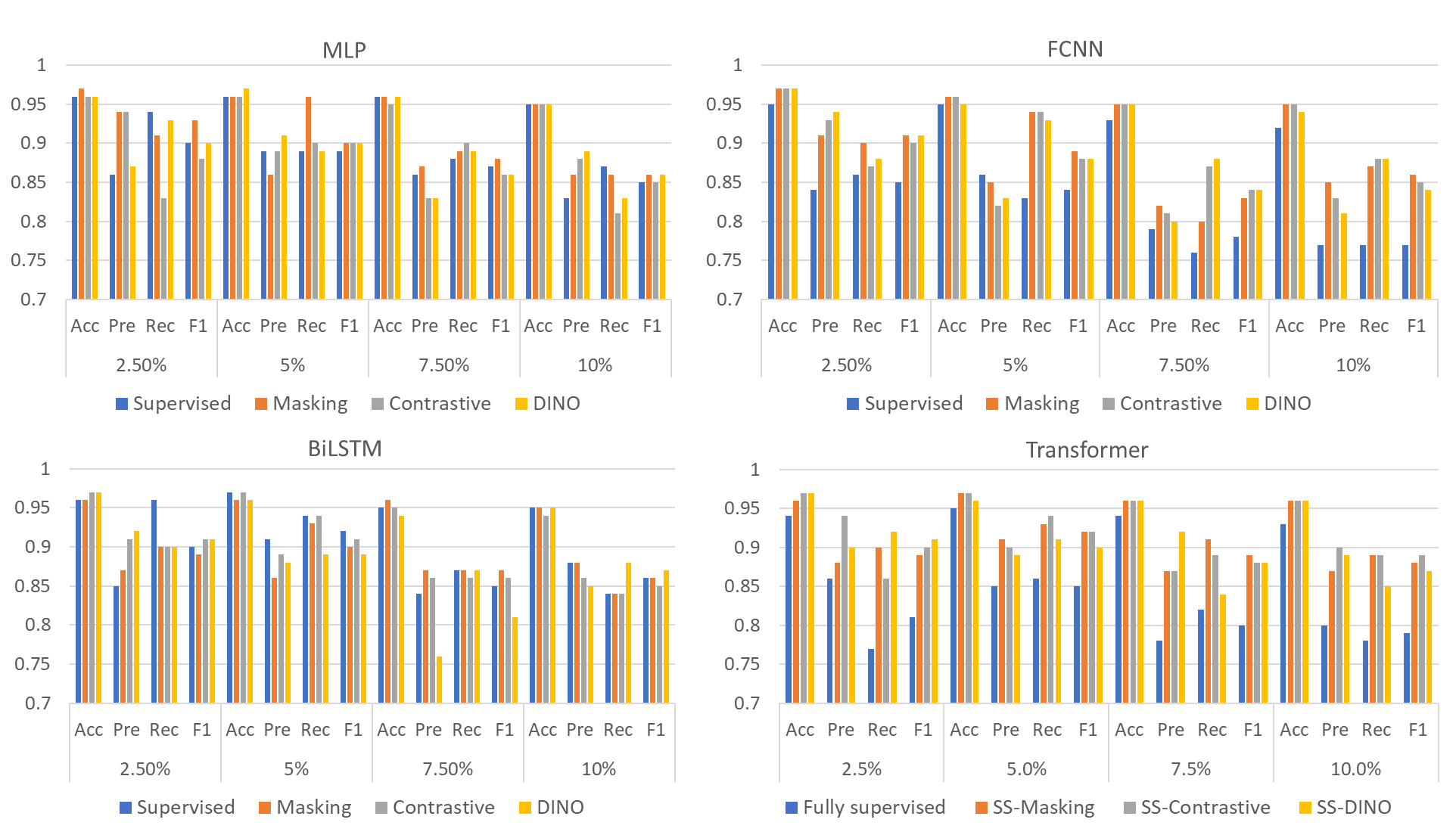
Figure 2: Classifier’s performance with different learning frameworks including fully-supervised, self-supervised learning with masking, contrastive, and DINO.

TABLE II: A comparison of self-supervised learning with different backbone

		2.5%				5%				7.5%				10%
Models		Acc	Pre	Rec	F1	Acc	Pre	Rec	F1	Acc	Pre	Rec	F1	Acc	Pre	Rec	F1
	MLP	0.96	0.86	0.94	0.90	0.96	0.89	0.89	0.89	0.96	0.86	0.88	0.87	0.95	0.83	0.87	0.85
	FCNN	0.95	0.84	0.86	0.85	0.95	0.86	0.83	0.84	0.93	0.79	0.76	0.78	0.92	0.77	0.77	0.77
	BiLSTM	0.96	0.85	0.96	0.90	0.97	0.91	0.94	0.92	0.95	0.84	0.87	0.85	0.95	0.88	0.84	0.86
Supervised	Transformer	0.94	0.86	0.77	0.81	0.95	0.85	0.86	0.85	0.94	0.78	0.82	0.80	0.93	0.80	0.78	0.79
	MLP	0.97	0.94	0.91	0.93	0.96	0.86	0.96	0.90	0.96	0.87	0.89	0.88	0.95	0.86	0.86	0.86
	FCNN	0.97	0.91	0.90	0.91	0.96	0.85	0.94	0.89	0.95	0.82	0.80	0.83	0.95	0.85	0.87	0.86
	BiLSTM	0.96	0.87	0.90	0.89	0.96	0.86	0.93	0.90	0.96	0.87	0.87	0.87	0.95	0.88	0.84	0.86
Masking	Transformer	0.96	0.88	0.90	0.89	0.97	0.91	0.93	0.92	0.96	0.87	0.91	0.89	0.96	0.87	0.89	0.88
	MLP	0.96	0.94	0.83	0.88	0.96	0.89	0.9	0.90	0.95	0.83	0.9	0.86	0.95	0.88	0.81	0.85
	FCNN	0.97	0.93	0.87	0.90	0.96	0.82	0.94	0.88	0.95	0.81	0.87	0.84	0.95	0.83	0.88	0.85
	BiLSTM	0.97	0.91	0.90	0.91	0.97	0.89	0.94	0.91	0.95	0.86	0.86	0.86	0.94	0.86	0.84	0.85
Contrastive	Transformer	0.97	0.94	0.86	0.90	0.97	0.90	0.94	0.92	0.96	0.87	0.89	0.88	0.96	0.90	0.89	0.89
	MLP	0.96	0.87	0.93	0.90	0.97	0.91	0.89	0.90	0.96	0.83	0.89	0.86	0.95	0.89	0.83	0.86
	FCNN	0.97	0.94	0.88	0.91	0.95	0.83	0.93	0.88	0.95	0.80	0.88	0.84	0.94	0.81	0.88	0.84
	BiLSTM	0.97	0.92	0.90	0.91	0.96	0.88	0.89	0.89	0.94	0.76	0.87	0.81	0.95	0.85	0.88	0.87
DINO	Transformer	0.97	0.90	0.92	0.91	0.96	0.89	0.91	0.90	0.96	0.92	0.84	0.88	0.96	0.89	0.85	0.87

The table II comprehensively evaluates various machine learning models across different learning paradigms and data proportions. It compares the performance of MLP, FCNN, BiLSTM, and Transformer models, each trained under fully supervised, masking, contrastive, and DINO self-supervised learning paradigms. The performance metrics include Accuracy (Acc), Precision (Pre), Recall (Rec), and F1 Score (F1), evaluated at four different ratios of annotated data: 2.5%, 5%, 7.5%, and 10%. Table II shows that the Transformer model, particularly when trained with SSL approaches like masking, contrastive, and DINO, consistently achieves high scores across all metrics, indicating its robustness and adaptability in learning from annotated and unannotated data. It significantly improves the Transformer’s performance compared to supervised learning cases. For example, under the DINO self-supervised paradigm, the Transformer model shows remarkable performance with an accuracy and F1 score of 0.97 and 0.91, respectively, at the 2.5% data ratio and maintains similar high performance across other data ratios. In contrast, while MLP and BiLSTM models perform best under fully supervised learning, their performance does not significantly improve with SSL techniques. The FCNN model, however, shows some improvement with SSL compared to fully supervised learning, but not to the extent seen with the Transformer model. Overall, these results underline the effectiveness of SSL, particularly with the Transformer model, in handling various proportions of annotated and unannotated data, outperforming traditional supervised methods and other neural network architectures like MLP, BiLSTM, and FCNN in terms of all evaluation metrics.

Moreover, from the visual data in Fig. 2, it is clear that the Transformer model consistently outperforms other models in SSL scenarios across all metrics and data proportions. Particularly under the contrastive paradigm, the Transformer model shows robust performance, often reaching peak scores. In contrast, while MLP and BiLSTM models exhibit strong performance in supervised learning, they do not exhibit the same improvement with SSL as the Transformer. FCNN shows a moderate improvement with SSL, suggesting that it benefits from these paradigms, but not as significantly as the Transformer. The trend across all models indicates that SSL, especially with the contrastive approach, substantially enhances model performance, with the Transformer model achieving notable improvements in learning from unannotated data and fine-tuning on annotated data. The bar charts serve as a clear visual testament to the advantages of employing SSL techniques in enhancing model robustness, with the Transformer model standing out as a particular architecture.

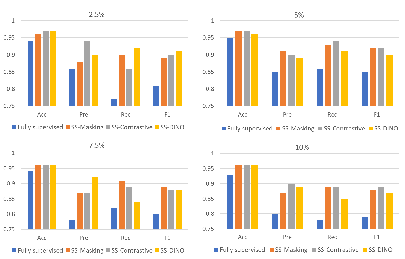
Figure 3: Transformer’s performance with different learning frameworks including fully-supervised, self-supervised learning with masking, contrastive, and DINO.

TABLE III: Transformer with self-supervised learning regarding different frameworks

	2.5%				5%				7.5%				10%
Models	Acc	Pre	Rec	F1	Acc	Pre	Rec	F1	Acc	Pre	Rec	F1	Acc	Pre	Rec	F1
Fully supervised	0.94	0.86	0.77	0.81	0.95	0.85	0.86	0.85	0.94	0.78	0.82	0.80	0.93	0.80	0.78	0.79
SS-Masking	0.96	0.88	0.90	0.89	0.97	0.91	0.93	0.92	0.96	0.87	0.91	0.89	0.96	0.87	0.89	0.88
SS-Contrastive	0.97	0.94	0.86	0.90	0.97	0.90	0.94	0.92	0.96	0.87	0.89	0.88	0.96	0.90	0.89	0.89
SS-DINO	0.97	0.90	0.92	0.91	0.96	0.89	0.91	0.90	0.96	0.92	0.84	0.88	0.96	0.89	0.85	0.87

Table III showcases a comparative analysis of the Transformer model’s efficacy when trained under different SSL frameworks—masking, contrastive, and DINO—relative to traditional fully supervised training. At the outset, with only 2.5% annotated data, the SSL models generally surpass the fully supervised model on all counts. The contrastive and DINO approaches, in particular, demonstrate marked improvements, with the contrastive framework achieving top scores for accuracy and F1. As we escalate the annotated data to 5% and 7.5%, the contrastive learning framework notably maintains its high scores, aligning with the DINO approach in terms of accuracy and F1, and consistently outshining the fully supervised model. Upon reaching 10% annotated data, this pattern persists, with SSL frameworks, especially the contrastive and DINO, proving more efficient than fully supervised learning. They register high F1, indicative of their capacity to effectively harness annotated and unannotated data.

Fig. 3 complements these findings with a visual representation, further illustrating the superiority of SSL, particularly in the contrastive learning and DINO variants, across varying levels of annotated data. Even with a mere 2.5% of data annotated, these SSL methods demonstrate significant enhancements in model performance, a trend that is sustained as the volume of annotated data grows. The contrastive approach, in particular, excels across the board, while DINO shows a strong balance between precision and recall, a critical factor in robust model training. The cumulative evidence from the table and figure underscores the robustness and efficiency of SSL frameworks, with the contrastive and DINO methods standing out. These SSL techniques not only improve the Transformer model’s performance in data-scarce situations but also exhibit remarkable adaptability and reliability across varied data availability scenarios, emphasizing the strengths of SSL in enhancing model performance.

TABLE IV: A comparison of contrastive loss from contrastive learning with Transformer

	2.5%				5%				7.5%				10%
Contrastive Loss	Acc	Pre	Rec	F1	Acc	Pre	Rec	F1	Acc	Pre	Rec	F1	Acc	Pre	Rec	F1
NT-Xent	0.97	0.94	0.86	0.90	0.97	0.90	0.94	0.92	0.96	0.87	0.89	0.88	0.96	0.90	0.89	0.89
SwCE	0͡.97	0.92	0.89	0.90	0.97	0.90	0.94	0.92	0.97	0.89	0.89	0.89	0.95	0.90	0.83	0.86
InfoNCE	0.96	0.90	0.90	0.90	0.97	0.91	0.93	0.92	0.96	0.87	0.89	0.88	0.96	0.88	0.87	0.87
Smooth InfoNCE	0.97	0.94	0.90	0.93	0.97	0.93	0.92	0.93	0.97	0.90	0.90	0.90	0.96	0.92	0.89	0.90

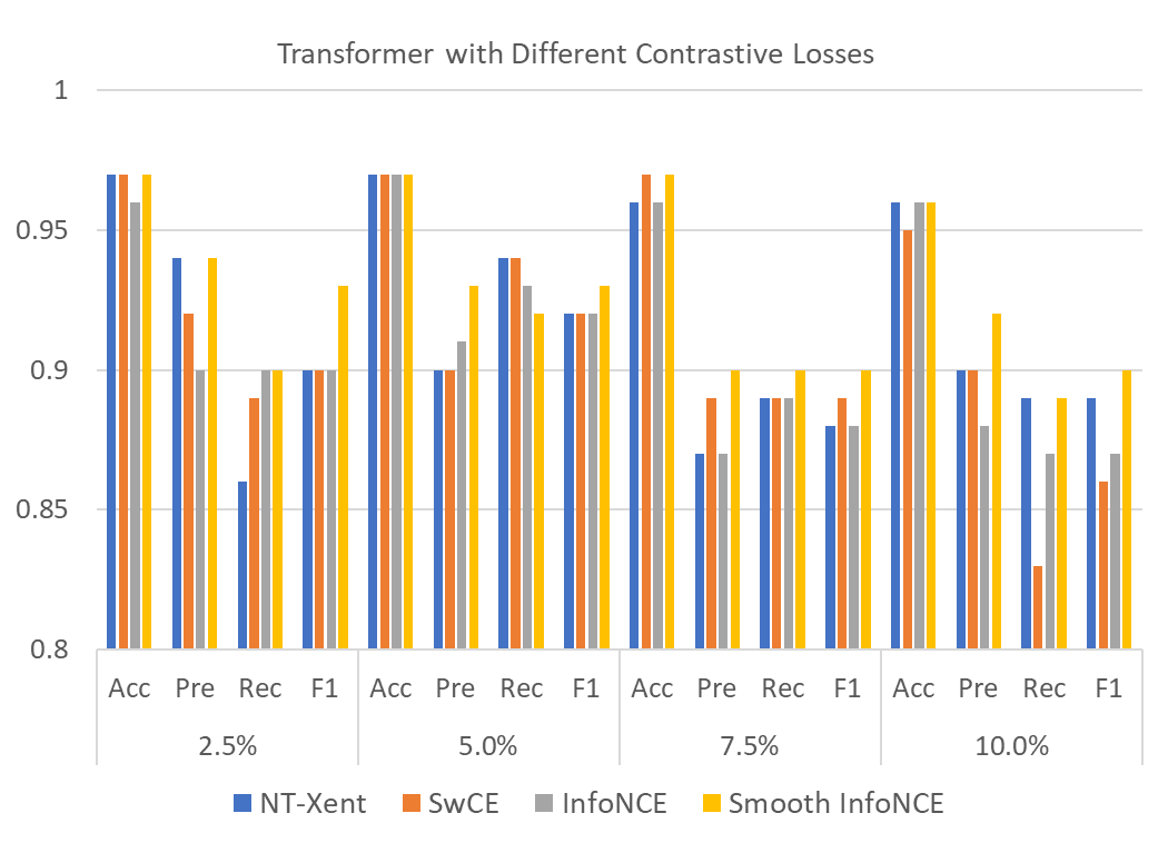
Figure 4: Contrastive self-supervised learning with different contrastive losses for Transformer.

Table IV evaluates the Transformer model using contrastive loss functions, including NT-Xent, SwCE, InfoNCE, and Smooth InfoNCE, revealing that with just 2.5% annotated data, NT-Xent and Smooth InfoNCE excel in accuracy and F1 score. As the annotated portion increases to 5% and 7.5%, these losses, along with SwCE, deliver top F1 scores, demonstrating a balanced precision-recall trade-off. At 10% annotation, they continue to showcase high accuracy and precision, with Smooth InfoNCE maintaining a notable F1 score. Synthesizing these insights, it is evident that contrastive loss functions significantly enhance the Transformer model’s performance, especially when annotated data is scarce. NT-Xent and Smooth InfoNCE, in particular, demonstrate consistent strength across all metrics, underlining their effectiveness within the Transformer’s contrastive learning framework.

Complementing Table IV, Figure 4 graphically shows the performance of the Transformer model under various contrastive losses. At the 2.5% annotation level, NT-Xent and Smooth InfoNCE manifest as superior performers. As the proportion of annotated data increases, these two losses retain their prominence, suggesting their efficacy in contexts with limited annotations. By the time annotated data reaches 10%, performances across the different loss functions begin to blend, with Smooth InfoNCE maintaining its strong precision, which could indicate a particular proficiency in generating confident predictions. Those results highlight the efficacy of contrastive loss functions in training Transformers, particularly in data-constrained environments. The consistently high performance of Smooth InfoNCE and NT-Xent suggests these methods are especially potent, showcasing the transformative potential of contrastive learning to boost Transformer models when resources are limited.

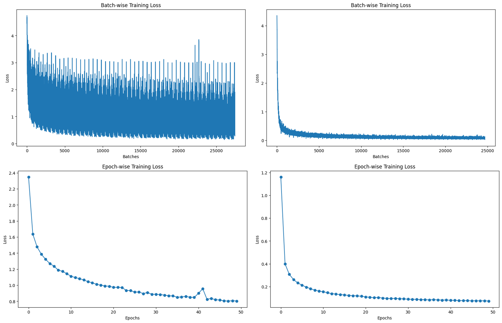
Figure 5: Training loss with InfoNCE (left) and SmoothInfoNCE (right) contrastive loss regarding to batches and epochs.

Additionally, Figure 5 presents a side-by-side comparison of the training loss for models utilizing InfoNCE and Smooth InfoNCE contrastive losses, with the left side depicting InfoNCE and the right side Smooth InfoNCE (with the fine-tunned $\lambda=0.75$). In the batch-wise training loss comparison, the InfoNCE loss exhibits high initial values and substantial fluctuation throughout training, suggesting some instability. Conversely, the Smooth InfoNCE demonstrates a quick reduction in loss, maintaining a lower and more stable trajectory, indicative of a steadier learning process. Epoch-wise, the InfoNCE loss graph shows an initial steep decline that gradually levels off, albeit with some irregularities that hint at ongoing learning adjustments. The Smooth InfoNCE’s epoch-wise loss, however, decreases consistently and without interruption, reflecting a more uniform and presumably more effective optimization over time. This overall comparison indicates that Smooth InfoNCE provides a more controlled and consistent reduction in training loss, both within batches and across epochs, potentially leading to better model generalization and performance stability.

Furthermore, motivated by adapting the unsupervised learning from Azar et al. [45], and our previous study [46], we continue to experiment with Transformer for different learning paradigms, including supervised, unsupervised, and self-supervised contrastive learning (with Smooth InfoNCE loss). Table V, and Fig. 6 present a comparative analysis of a Transformer model’s performance across three learning paradigms: supervised, unsupervised (using Autoencoders, AE), and self-supervised. Across all metrics, self-supervised learning exhibits consistently high performance, particularly excelling over supervised learning. Even with a minimal 2.5% of annotated data, self-supervised learning matches the top accuracy and precision shown by unsupervised learning while significantly surpassing supervised learning, especially in recall and F1 scores. As the amount of annotated data increases, the self-supervised Transformer maintains its superiority over supervised learning and demonstrates marked improvements over the unsupervised AE approach. This trend is consistent with up to 10% annotated data, where self-supervised learning still shows the highest metrics, confirming its effectiveness in leveraging both labeled and unlabeled data to improve performance, particularly in scenarios with limited annotations.

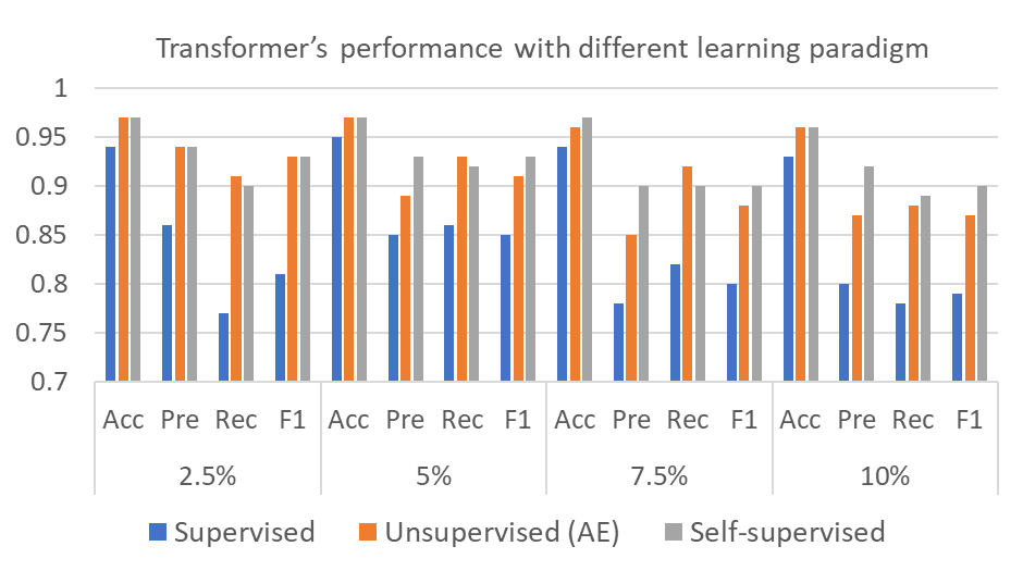
Figure 6: Transformer’s performance with different learning paradigms including supervised, unsupervised (AE), and self-supervised contrastive learning (SmoothInfoNCE).

TABLE V: A comparison of Transformer’s performance with different learning paradigm

Transformer	2.5%				5%				7.5%				10%
	Acc	Pre	Rec	F1	Acc	Pre	Rec	F1	Acc	Pre	Rec	F1	Acc	Pre	Rec	F1
Supervised	0.94	0.86	0.77	0.81	0.95	0.85	0.86	0.85	0.94	0.78	0.82	0.80	0.93	0.80	0.78	0.79
Unsupervised (AE)	0.97	0.94	0.91	0.93	0.97	0.89	0.93	0.91	0.96	0.85	0.92	0.88	0.96	0.87	0.88	0.87
Self-supervised	0.97	0.94	0.90	0.93	0.97	0.93	0.92	0.93	0.97	0.90	0.90	0.90	0.96	0.92	0.89	0.90

V Conclusion

In the specialized context of PPG signal analysis for PICU applications, this investigation champions SSL as an innovative method to capitalize on the abundant yet underutilized unlabeled data. Through the adoption of SSL, the study has notably enhanced the Transformer model’s capacity to interpret signal characteristics, thereby improving its accuracy in the detection of PPG artifacts. The spectrum of SSL techniques explored—masking, contrastive learning, and DINO—revealed contrastive learning as the standout strategy, exhibiting remarkable efficacy, particularly with limited datasets.

The study further delves into the nuanced domain of contrastive learning, focusing on refining loss functions essential to SSL’s efficacy. Inspired by the foundational InfoNCE loss, a novel loss function has been devised to facilitate more stable training and superior convergence, subsequently boosting the Transformer’s performance in artifact identification tasks.

The research validates SSL’s potential to enhance neural network models’ performance, such as the Transformer, by effectively utilizing unlabeled data. This approach shows significant promise for deployment in environments like the PICU, where annotated data is a rarity. The study marks a critical evolution in machine learning, empirically validating the speculated advantages of SSL techniques over conventional supervised and unsupervised learning in enriching model performance and knowledge acquisition.

Thanh-Dung Le (Member, IEEE) received a B.Eng. degree in mechatronics engineering from Can Tho University, Vietnam, an M.Eng. degree in electrical engineering from Jeju National University, S. Korea, and a Ph.D. in biomedical engineering from École de Technologie Supérieure (ETS), Canada. He is a postdoctoral fellow at the Biomedical Information Processing Laboratory, ETS. His research interests include applied machine learning approaches for biomedical informatics problems. Before that, he joined the Institut National de la Recherche Scientifique, Canada, where he researched classification theory and machine learning with healthcare applications. He received the merit doctoral scholarship from Le Fonds de Recherche du Quebec Nature et Technologies. He also received the NSERC-PERSWADE fellowship, Canada, and a graduate scholarship from the Korean National Research Foundation, S. Korea.

Clara Macabiau is a double degree student in Canada. After three years at the École nationale supérieure d’électrotechnique, d’électronique, d’informatique, d’hydraulique et des télécommunications (ENSEEIHT) engineering school in Toulouse, she is completing her master’s degree in electrical engineering at École de Technologie Supérieure (ETS), Canada. Her master’s project focuses on the detection of artifacts in photoplethysmography signals. She interests in signal processing, machine learning, and electronics.

Kevin Albert is a physiotherapist who graduated from EUSES School of Health and Sport (2018 - Girona, Spain). He developed clinical expertise in the field of function rehabilitation after neuro-traumatic injury (France) and in cardio-respiratory rehabilitation (Swiss). He is currently enrolled in the Master’s Biomedical Engineering program at the University of Montreal and has joined the Clinical Decision Support System (CDSS) laboratory under the supervision of Prof. P. Jouvet, M.D. Ph.D. in the Pediatric Intensive Care Unit at Sainte-Justine Hospital (Montréal, Canada) since May 2023. His primary research interest is the application of new technologies of support care system tools with artificial intelligence, especially in ventilatory support. His research program is supported by the Sainte-Justine Hospital and the Quebec Respiratory Health Research Network (QRHN).

Philippe Jouvet received the M.D. degree from Paris V University, Paris, France, in 1989, the M.D. specialty in pediatrics and the M.D. subspecialty in intensive care from Paris V University, in 1989 and 1990, respectively, and the Ph.D. degree in pathophysiology of human nutrition and metabolism from Paris VII University, Paris, in 2001. He joined the Pediatric Intensive Care Unit of Sainte Justine Hospital—University of Montreal, Montreal, QC, Canada, in 2004. He is currently the Deputy Director of the Research Center and the Scientific Director of the Health Technology Assessment Unit, Sainte Justine Hospital–University of Montreal. He has a salary award for research from the Quebec Public Research Agency (FRQS). He currently conducts a research program on computerized decision support systems for health providers. His research program is supported by several grants from the Sainte-Justine Hospital, Quebec Ministry of Health, the FRQS, the Canadian Institutes of Health Research (CIHR), and the Natural Sciences and Engineering Research Council (NSERC). He has published more than 160 articles in peer-reviewed journals. Dr. Jouvet gave more than 120 lectures in national and international congresses.

Rita Noumeir (Member, IEEE) received master’s and Ph.D. degrees in biomedical engineering from École Polytechnique of Montreal. She is currently a Full Professor with the Department of Electrical Engineering, École de Technologie Superieure (ETS), Montreal. Her main research interest is in applying artificial intelligence methods to create decision support systems. She has extensively worked in healthcare information technology and image processing. She has also provided consulting services in large-scale software architecture, healthcare interoperability, workflow analysis, and technology assessment for several international software and medical companies, including Canada Health Infoway.

References

- [1] D. Brossier, R. El Taani, M. Sauthier, N. Roumeliotis, G. Emeriaud, and P. Jouvet, “Creating a high-frequency electronic database in the picu: the perpetual patient,” Pediatr. Crit. Care Med., vol. 19, no. 4, pp. e189–e198, 2018.
- [2] N. Roumeliotis, G. Parisien, S. Charette, E. Arpin, F. Brunet, and P. Jouvet, “Reorganizing care with the implementation of electronic medical records: a time-motion study in the picu,” Pediatr. Crit. Care Med., vol. 19, no. 4, pp. e172–e179, 2018.
- [3] A. Mathieu and et. al., “Validation process of a high-resolution database in a pediatric intensive care unit—describing the perpetual patient’s validation,” Journal of Evaluation in Clinical Practice, vol. 27, no. 2, pp. 316–324, 2021.
- [4] A. C. Dziorny and et. al., “Clinical decision support in the picu: Implications for design and evaluation,” Pediatr. Crit. Care Med., vol. 23, no. 8, pp. e392–e396, 2022.
- [5] T.-D. Le and et. al., “Detecting of a patient’s condition from clinical narratives using natural language representation,” IEEE Open J. Eng. Med. Biol., vol. 3, pp. 142–149, 2022.
- [6] M. Sauthier, G. Tuli, P. A. Jouvet, J. S. Brownstein, and A. G. Randolph, “Estimated pao2: A continuous and noninvasive method to estimate pao2 and oxygenation index,” Critical care explorations, vol. 3, no. 10, 2021.
- [7] G. Emeriaud, Y. M. López-Fernández, N. P. Iyer, M. M. Bembea, A. Agulnik, R. P. Barbaro, F. Baudin, A. Bhalla, W. B. De Carvalho, C. L. Carroll, et al., “Executive summary of the second international guidelines for the diagnosis and management of pediatric acute respiratory distress syndrome (palicc-2),” Pediatr. Crit. Care Med., vol. 24, no. 2, p. 143, 2023.
- [8] P. Jouvet and et. al., “A pilot prospective study on closed loop controlled ventilation and oxygenation in ventilated children during the weaning phase,” Critical Care, vol. 16, no. 3, pp. 1–9, 2012.
- [9] M. Wysocki, P. Jouvet, and S. Jaber, “Closed loop mechanical ventilation,” J. Clin. Monit. Comput., vol. 28, pp. 49–56, 2014.
- [10] B. L. Hill and et. al., “Imputation of the continuous arterial line blood pressure waveform from non-invasive measurements using deep learning,” Scientific reports, vol. 11, no. 1, p. 15755, 2021.
- [11] F. Fan and et. al., “Estimating spo 2 via time-efficient high-resolution harmonics analysis and maximum likelihood tracking,” IEEE J. Biomed. Health Inform., vol. 22, no. 4, pp. 1075–1086, 2017.
- [12] C. Macabiau, T.-D. Le, K. Albert, P. Jouvet, and R. Noumeir, “Label propagation techniques for artifact detection in imbalanced classes using photoplethysmogram signals,” arXiv preprint arXiv:2308.08480, 2023.
- [13] T.-D. Le, C. Macabiau, K. Albert, P. Jouvet, and R. Noumeir, “Grn-transformer: Enhancing motion artifact detection in picu photoplethysmogram signals,” arXiv preprint arXiv:2308.03722, 2023.
- [14] E. Khan, F. Al Hossain, S. Z. Uddin, S. K. Alam, and M. K. Hasan, “A robust heart rate monitoring scheme using photoplethysmographic signals corrupted by intense motion artifacts,” IEEE Transactions on Biomedical engineering, vol. 63, no. 3, pp. 550–562, 2015.
- [15] D. Dao and et. al., “A robust motion artifact detection algorithm for accurate detection of heart rates from photoplethysmographic signals using time-frequency spectral features,” IEEE J. Biomed. Health Inform, vol. 21, no. 5, pp. 1242–1253, 2016.
- [16] P. Mehrgardt and et. al., “Deep learning fused wearable pressure and ppg data for accurate heart rate monitoring,” IEEE Sensors Journal, vol. 21, no. 23, pp. 27 106–27 115, 2021.
- [17] J. Liu and et. al., “Pca-based multi-wavelength photoplethysmography algorithm for cuffless blood pressure measurement on elderly subjects,” IEEE J. Biomed. Health Inform, vol. 25, no. 3, pp. 663–673, 2020.
- [18] D. A. Birrenkott and et. al., “A robust fusion model for estimating respiratory rate from photoplethysmography and electrocardiography,” IEEE Trans. Biomed. Eng., pp. 2033–2041, 2017.
- [19] B. Venema and et. al., “Robustness, specificity, and reliability of an in-ear pulse oximetric sensor in surgical patients,” IEEE J. Biomed. Health Inform, vol. 18, no. 4, pp. 1178–1185, 2013.
- [20] E. A. Alharbi and et. al., “Non-invasive solutions to identify distinctions between healthy and mild cognitive impairments participants,” IEEE J. Transl. Eng. Health Med., vol. 10, pp. 1–6, 2022.
- [21] C. Nwibor and et. al., “Remote health monitoring system for the estimation of blood pressure, heart rate, and blood oxygen saturation level,” IEEE Sensors Journal, vol. 23, no. 5, pp. 5401–5411, 2023.
- [22] Z. Wang and et. al., “Time series classification from scratch with deep neural networks: A strong baseline,” in International joint conference on neural networks, 2017, pp. 1578–1585.
- [23] D. Marzorati and et. al., “Hybrid convolutional networks for end-to-end event detection in concurrent ppg and pcg signals affected by motion artifacts,” IEEE Trans. Biomed. Eng., vol. 69, no. 8, 2022.
- [24] S. Maqsood and et. al., “A benchmark study of machine learning for analysis of signal feature extraction techniques for blood pressure estimation using photoplethysmography (ppg),” Ieee Access, vol. 9, pp. 138 817–138 833, 2021.
- [25] D. Hendrycks, M. Mazeika, S. Kadavath, and D. Song, “Using self-supervised learning can improve model robustness and uncertainty,” Advances in neural information processing systems, vol. 32, 2019.
- [26] T. Lin and et. al., “A survey of transformers,” AI Open, 2022.
- [27] T.-D. Le and et. al., “A small-scale switch transformer and nlp-based model for clinical narratives classification,” arXiv preprint arXiv:2303.12892, 2023.
- [28] R. Shwartz-Ziv, R. Balestriero, K. Kawaguchi, T. G. Rudner, and Y. LeCun, “An information-theoretic perspective on variance-invariance-covariance regularization,” arXiv preprint arXiv:2303.00633, 2023.
- [29] J. Devlin and et. al., “Bert: Pre-training of deep bidirectional transformers for language understanding,” in Proceedings of the 2019 Conference of the North American Chapter of the Association for Computational Linguistics: Human Language Technologies, Volume 1 (Long and Short Papers), 2019, pp. 4171–4186.
- [30] P. H. Le-Khac, G. Healy, and A. F. Smeaton, “Contrastive representation learning: A framework and review,” Ieee Access, vol. 8, pp. 193 907–193 934, 2020.
- [31] T. Chen, S. Kornblith, M. Norouzi, and G. Hinton, “A simple framework for contrastive learning of visual representations,” in International conference on machine learning. PMLR, 2020, pp. 1597–1607.
- [32] K. Sohn, “Improved deep metric learning with multi-class n-pair loss objective,” Advances in neural information processing systems, vol. 29, 2016.
- [33] A. v. d. Oord, Y. Li, and O. Vinyals, “Representation learning with contrastive predictive coding,” arXiv preprint arXiv:1807.03748, 2018.
- [34] M. Caron, I. Misra, J. Mairal, P. Goyal, P. Bojanowski, and A. Joulin, “Unsupervised learning of visual features by contrasting cluster assignments,” Advances in neural information processing systems, vol. 33, pp. 9912–9924, 2020.
- [35] M. Caron, H. Touvron, I. Misra, H. Jégou, J. Mairal, P. Bojanowski, and A. Joulin, “Emerging properties in self-supervised vision transformers,” in Proceedings of the IEEE/CVF international conference on computer vision, 2021, pp. 9650–9660.
- [36] F. Pedregosa and et. al, “Scikit-learn: Machine learning in Python,” Journal of Machine Learning Research, vol. 12, pp. 2825–2830, 2011.
- [37] F. Chollet and et. al., “keras,” 2015.
- [38] D. Hunter and et. al., “Selection of proper neural network sizes and architectures—a comparative study,” IEEE Transactions on Industrial Informatics, vol. 8, no. 2, pp. 228–240, 2012.
- [39] M. Popel and et. al., “Training tips for the transformer model,” arXiv preprint arXiv:1804.00247, 2018.
- [40] N. Srivastava and et. al., “Dropout: a simple way to prevent neural networks from overfitting,” The journal of machine learning research, vol. 15, no. 1, pp. 1929–1958, 2014.
- [41] X. Glorot and et. al., “Understanding the difficulty of training deep feedforward neural networks,” in Proceedings of the thirteenth international conference on artificial intelligence and statistics. JMLR Workshop and Conference Proceedings, 2010, pp. 249–256.
- [42] S. Ioffe and et. al., “Batch normalization: Accelerating deep network training by reducing internal covariate shift,” in International Conference on Machine Learning. PMLR, 2015, pp. 448–456.
- [43] N. Bjorck and et. al., “Understanding batch normalization,” Advances in Neural Information Processing Systems, vol. 31, 2018.
- [44] H. He and et. al., “Adasyn: Adaptive synthetic sampling approach for imbalanced learning,” in IEEE international joint conference on neural networks, 2008, pp. 1322–1328.
- [45] J. Azar and et. al., “Deep recurrent neural network-based autoencoder for photoplethysmogram artifacts filtering,” Computers & Electrical Engineering, vol. 92, p. 107065, 2021.
- [46] T.-D. Le, R. Noumeir, J. Rambaud, G. Sans, and P. Jouvet, “Adaptation of autoencoder for sparsity reduction from clinical notes representation learning,” IEEE Journal of Translational Engineering in Health and Medicine, 2023.