Fast Inference Through The Reuse Of Attention Maps In Diffusion Models

Abstract

Text-to-image diffusion models have demonstrated unprecedented abilities at flexible and realistic image synthesis. However, the iterative process required to produce a single image is costly and incurs a high latency, prompting researchers to further investigate its efficiency. Typically, improvements in latency have been achieved in two ways: (1) training smaller models through knowledge distillation (KD); and (2) adopting techniques from ODE-theory to facilitate larger step sizes. In contrast, we propose a training-free approach that does not alter the step-size of the sampler. Specifically, we find the repeated calculation of attention maps to be both costly and redundant; therefore, we propose a structured reuse of attention maps during sampling. Our initial reuse policy is motivated by rudimentary ODE-theory, which suggests that reuse is most suitable late in the sampling procedure. After noting a number of limitations in this theoretical approach, we empirically search for a better policy. Unlike methods that rely on KD, our reuse policies can easily be adapted to a variety of setups in a plug-and-play manner. Furthermore, when applied to Stable Diffusion-1.5, our reuse policies reduce latency with minimal repercussions on sample quality.

1 Introduction

Diffusion probabilistic models (DPMs) have become increasingly popular for text-conditioned image generation [21, 5, 19, 23]. Although their performance is unprecedented, they are still relatively slow. This has prompted interest in methods for reducing their latency. These methods can be lumped into two categories: (1) decrease the number of calls to the U-net, and (2) decrease the cost of calling the U-net. However, reducing the cost or number of calls to the U-net will degrade sample quality by increasing the discretization or approximation error, respectively.

For a small step-size (large number of functional evaluations - NFEs) the approximation error dominates the discretization error [28]. In this case, the discretization error shouldn’t be a limiting factor for sample quality. Therefore, in the large-NFE regime, increasing the step-size is a sensible approach for reducing DPM latency. This increase in step-size can be extended by the use of additional tricks such as knowledge distillation (KD) [24] or sophisticated sampling procedures [15]. In contrast, in the low-NFE regime, the discretization error is larger, which makes further increases in step-size harmful to sample quality. Notably, methods designed to reduce latency while retaining step-size have received relatively little attention.

Our paper focuses on this gap, retaining step-size and directly reducing the cost of calling the U-net instead. We achieve this by removing an expensive aspect of the sampling procedure that we find may sometimes be redundant: the repeated calculation of attention maps. Specifically, instead of recalculating attention maps from the key-query pairs at each step, the most recently calculated attention maps are stored in memory and can be reused during the sampling procedure. An uninformed choice of attention-reuse policy (i.e., the steps where attention maps are to be reused) unacceptability reduces model performance, as demonstrated in Figure 1. As such, the main contribution of our paper is locating and explaining the most appropriate attention-reuse policies. We achieve this as follows:

• We start by locating a base policy by analysing the Lyapunov exponents of the reverse diffusion ODE.

• To remedy the deficits of this base policy, we searched to find a policy with the same latency but greater efficacy.

• Finally, we show that our reuse policies outperform step-reduced samplers of comparable latency.

	DDIM(20)	PHAST	Policy A	Policy B	Policy C	Policy D	Policy E
Laptop Computer
English Setter
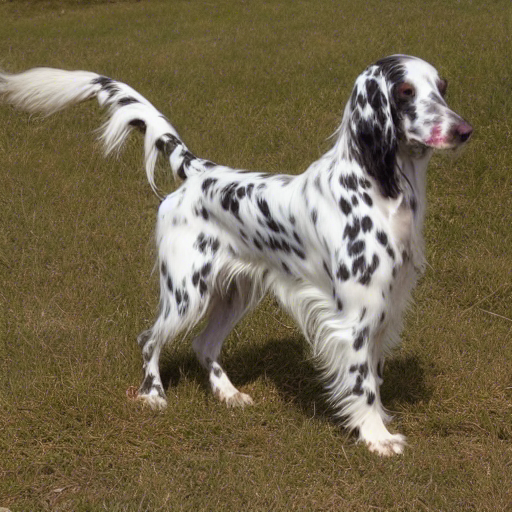
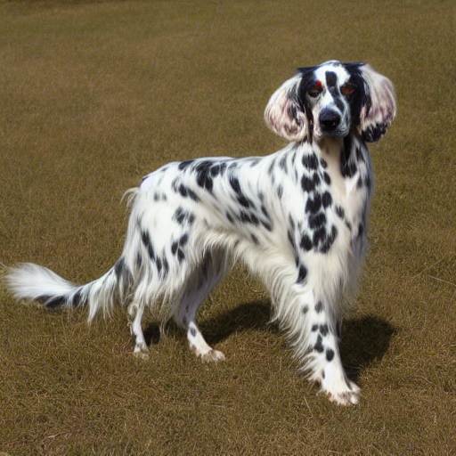
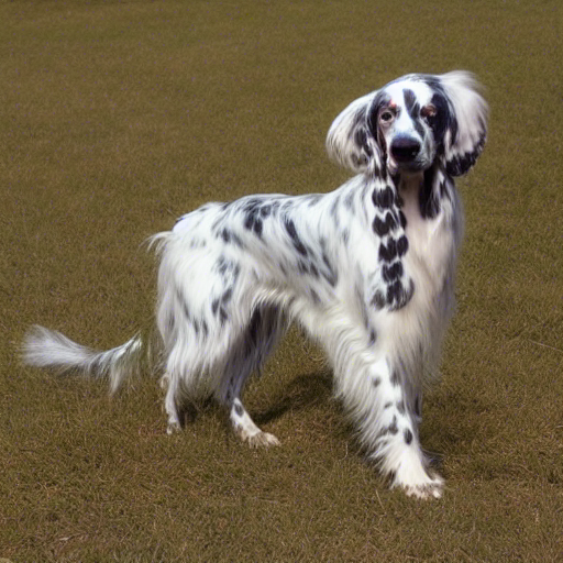
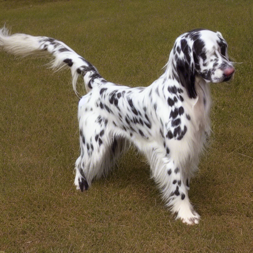
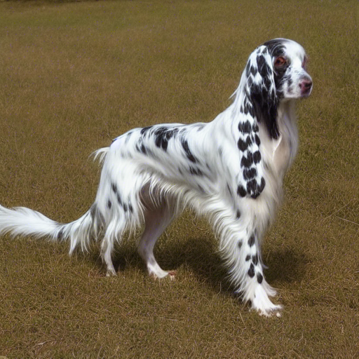
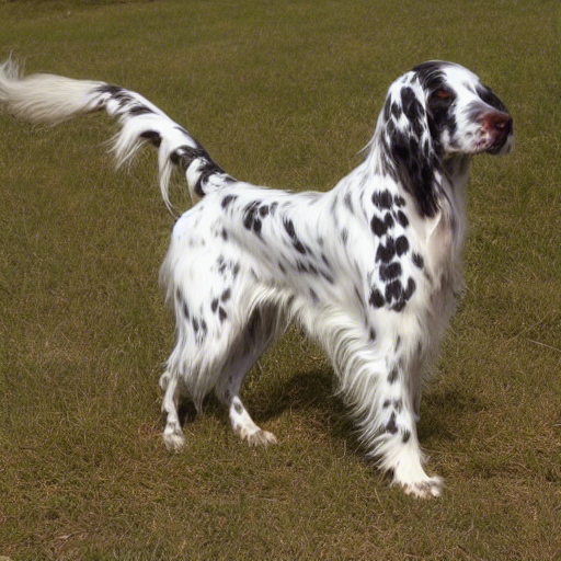
Sealyham Terrier

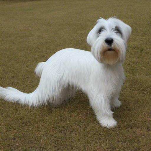
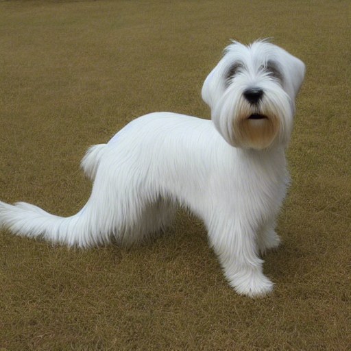
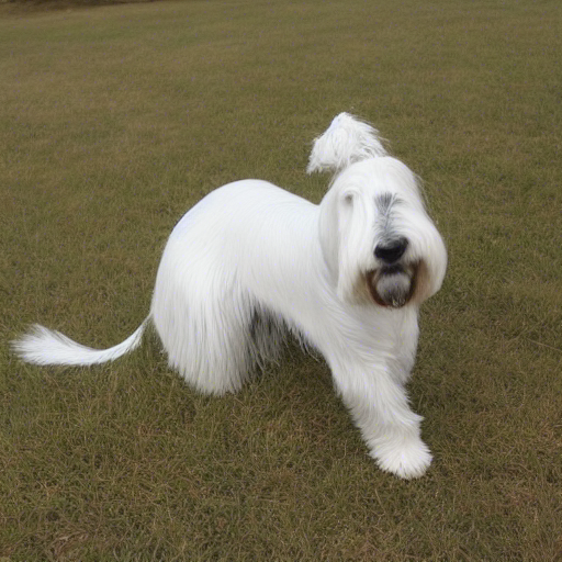
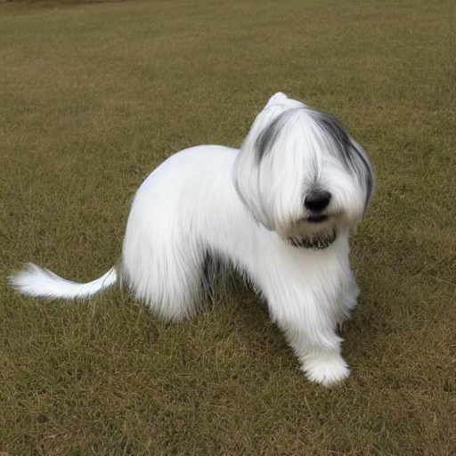
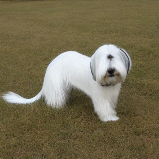
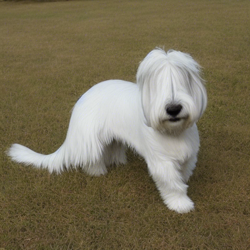
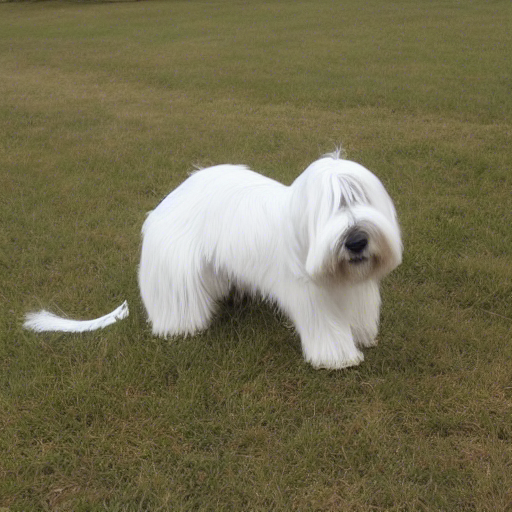
Figure 1: Comparison of a baseline 20-step DDIM with five stochastic attention-reuse policies (A-E) in which a random ten steps are selected for reuse. We also include our best 10-step reuse policy (PHAST) to demonstrate that good reuse policies do exist. The exact prompts are taken from ImageNet [4]: ‘laptop, laptop computer’; ‘English Setter’; ‘Sealyham terrier Sealyham’.

2 Related Work

Sampling from a Diffusion Model. The noising process in diffusion models results from the iterative application of encoders [17]. These encoders have pre-determined parameters, defined such that they transform any input image, $\boldsymbol{x}_{0}$, approximately into a standard Gaussian by the final timestep, $\boldsymbol{x}_{T}$. In the reverse direction, de-noising involves repeatedly invoking a decoder, which is typically trained to predict a score function, $\nabla_{\boldsymbol{x}}\text{log }q_{t}(\boldsymbol{x}_{t})$. This is either learned directly, $\boldsymbol{s}_{\theta}\left(\boldsymbol{x}_{t},t\right)$, or indirectly via error estimation, $\boldsymbol{\epsilon}_{\theta}\left(\boldsymbol{x}_{t},t\right)$. Once the network is trained, the model must be paired with a sampling procedure that uses information from the decoder to reproduce $\boldsymbol{x}_{0}$ from $\boldsymbol{x}_{T}$, potentially with the aid of a prompt. This reverse diffusion process is often modelled by a stochastic differential equation (SDE) [9] or an ordinary differential equation (ODE) [26]:

$$d\boldsymbol{x}_{t}=\left[f(t)\boldsymbol{x}_{t}-g^{2}(t)\nabla_{\boldsymbol{x}}\text{log }q_{t}(\boldsymbol{x}_{t})\right]dt+g(t)d\overline{\boldsymbol{w}}_{t}$$ (1)

$$d\boldsymbol{x}_{t}=f(t)\boldsymbol{x}_{t}-\frac{1}{2}g^{2}(t)\nabla_{\boldsymbol{x}}\text{log }q_{t}(\boldsymbol{x}_{t})dt,$$ (2)

where $f(t)$, $g(t)$ are determined by the noise schedule and $\overline{\boldsymbol{w}}_{t}$ is a standard Wiener process in reverse time. Successfully solving either of these equations corresponds to the DPM sampling a realistic image. One approach [20] to solving the SDE involves augmenting Euler’s method with the injection of Gaussian noise of variance $\Delta t$ at each timestep. This noise facilitates error contraction [28] but hinders convergence for large step sizes. Alternatively, ODE-solvers [25] are more suited to large step sizes because their flow is deterministic upon initialisation. However, ODE-solvers are still rather slow, thus motivating the research community to investigate low-latency DPMs.

Decreasing the Number of U-Net Calls. One approach to DPM latency is to simply reduce the number of times that the U-net is called — reduce the NFEs. A naive reduction to the NFEs, by simply reducing the number of steps, would increase discretization error and degrade sample quality. A typical way to retain model performance is knowledge distillation, in which a student network that requires fewer NFEs is trained to emulate the (teacher) original DPM. For example, progressive distillation [24, 18] involves iteratively training a student network to predict, in one-step, a teacher model’s two-step output, repeatedly halving the NFEs. Since then, a variety of new methods have been proposed to extend this simple approach. Some researchers [27, 7, 2] have expanded on progressive distillation, producing single-step solvers that generate (or sample from) any point along the whole diffusion trajectory. Alternatively, InstaFlow [14] directly reduced the curvature of diffusion trajectories. This enables larger step-sizes as trajectory curvature is closely linked to discretization error.

All of the methods listed above reduce latency with a minimal impact on sample quality; however, they require some form of training and, as such, can’t directly bolster pre-trained DPMs. Another paradigm for reducing the number of U-net calls is to improve the underlying ODE-solver. For example, Lu et al. [15] produced an analytic solution to the reverse diffusion ODE that involves an exponentially weighted integral. From this, they derived a (potentially high-order) numerical method that approximates the Taylor expansion of the exponential integral. A high-order solver is able to track the curvature of diffusion trajectories [6], enabling a larger step-size. Unlike the approaches that require KD, sophisticated sampling procedures can be directly applied to pre-trained DPMs in a ‘plug-and-play’ [15] manner.

Decreasing the Cost of U-Net Calls. Another approach to improving DPM latency is reducing the cost of a functional evaluation by making the U-net leaner. Analogous to the use of KD above, sample quality can be retained by training a student network with fewer components to emulate an existing U-net. Kim et al. [8] manually removed blocks from the U-net in Stable Diffusion [22] and used this pruned model as a student of the original U-net. Li et al. [11] developed this manual approach by pruning the U-net in accordance with a formalised trade-off between performance (CLIP-score) and latency. Both of these papers retain sample quality by employing KD, but can the cost of calling a U-net be reduced without retraining?

In the related area of Transformers, Bhojanapalli et al. [3] improved latency by exploiting redundancies in the repeated calculation of attention maps. These maps are particularly consequential for latency as their calculation involves a costly outer product between a high-dimensional key and query. Upon finding a reasonable degree of similarity between a Transformer’s attention maps, they reused an arbitrary subset of the maps from layer 1 in the following layers. We wonder whether similar redundancies exist in the attention maps produced in diffusion models, and if so, whether this can equally be exploited through reuse to reduce the cost of calling the U-net in DPMs.

3 Analysis

We begin this section by estimating the extent to which the repeated calculation of attention maps exhibits redundancy in DPMs. Upon finding a significant degree of redundancy, we then move towards defining and locating successful reuse policies that optimally exploit this redundancy. The policy produced in this section, HURRY, is derived from a general theoretical approach (Lyapunov exponents) that probes the dynamics of error propagation in DPMs. Unless otherwise stated, all figures and tables are run using Stable Diffusion v1.5 with a 20-step DDIM [25] acting as the base sampler.

Attention Map Redundancy. We conjecture that DPM attention maps are, predictably, similar to their temporally adjacent neighbours during sampling. As such, we empirically investigate the normalised L1 difference [3] between these maps, averaged over a variety of prompts. Figure 2 illustrates a high degree of similarity, in which temporally adjacent maps are (on average) within 0.2 of each other. This suggests a relatively stable degree of redundancy in the repeated calculation of attention maps that can be exploited to reduce latency. Specifically, instead of repeatedly calculating highly similar maps directly from key-query pairs, certain attention maps can be used more than once. But what exactly would this look like?

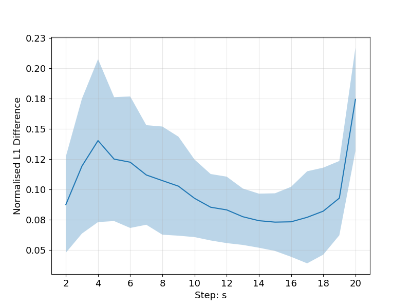
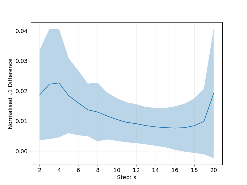
Figure 2: Normalised L1-distance between the Self- (left) and Cross- (right) attention maps A(s) and A(s-1) for an unperturbed flow. This is generated from twenty random ImageNet prompts using a 20-step DDIM-sampler. The shaded region includes one standard deviation.

Defining Reuse and Success. Before we continue, we must first concretely define what is even meant by reuse. Each layer ($l$) and step ($s$) in the diffusion process has a corresponding attention map ($\boldsymbol{A}_{s}^{l}$) that can be directly calculated from key-query pairs. We define layer-wise memory variables ($\boldsymbol{M}^{l}$) that store the maps that we may wish to reuse. During sampling, we let $\boldsymbol{M}^{l}\leftarrow\boldsymbol{A}_{s}^{l}$ at each step-layer pair, in which we directly calculate an attention map. For a reuse step $r>1$, we let $\boldsymbol{A}_{r}^{l}\leftarrow\boldsymbol{M}^{l}$, instead of directly calculating $\boldsymbol{A}_{r}^{l}$ from key-query pairs.

Now that we have a notion of what reuse involves, it may also be helpful to define when reuse is successful. In this paper, we will define a reuse policy as successful if each of its samples is close to the corresponding sample from the original (no-reuse) flow. An alternative (distributional) characterisation of success would require that the samples have a good CLIP-Score or FID with an external dataset.

In the evaluation section, we will present results regarding both characterisations of success. However, when performing our analysis and search algorithms, we use the sample-by-sample definition of success for three main reasons. First, it’s less subjective than the distributional measures of success, which are contingent on a choice of dataset. Second, unlike the distribution approaches, it facilitates the use of Lyapunov exponents to probe error propagation in DPMs. Finally, the difference between two samples can be calculated quickly, facilitating faster search algorithms.

Locating a Successful Reuse Policy. A naive way of locating an optimal reuse strategy would be to trial every policy and search for the one whose output most closely approximates the true sample. However, an exhaustive search is infeasible due to the exponential growth in the number of policies as the number of steps increases. Therefore, we probe the diffusion process for information that can warm-up our search. One probe into dynamical systems ($\textbf{z}_{t}$) are ‘Lyapunov exponents’ [10] which assume that errors ($\delta\textbf{z}_{t}$) grow (or shrink) exponentially in time. Formally, they assume there exists a $k\in\mathbb{R}\backslash\{0\}$ such that for every $t>\tau>0$:

$$\left|\delta\textbf{z}_{t}\right|\approx e^{k\tau}\left|\delta\textbf{z}_{t-\tau}\right|.$$ (3)

Let $\boldsymbol{x}_{t}$ represent the reverse diffusion process, where $\boldsymbol{x}_{0}$ is Gaussian noise and $\boldsymbol{x}_{T}$ is a sample. Furthermore, let $\textbf{A}_{s}$ denote the attention maps at sampling step s. Adapting our formalisation of Lyapunov exponents into a model of DPM dynamics where attention maps are perturbed, we conjecture that there exists a $\lambda>0$ such that for every step, $s\in\mathbb{N}$ and corresponding timestep $T>t_{s}>0$:

$$\left|\delta\boldsymbol{x}_{T}\right|\propto e^{\lambda(T-t_{s})}\left|\delta\textbf{A}_{s}\right|\propto e^{-\lambda t_{s}}\left|\delta\textbf{A}_{s}\right|.$$ (4)

That is, the change in the sample ($\delta\boldsymbol{x}_{T}$) is proportional to the change in the attention maps ($\delta\textbf{A}_{s}$) introduced by reuse at step $s$, subject to an exponential growth over the remaining steps. If our conjecture is true, then a heuristic policy that follows from this would be to reuse (i.e., perturb the attention map) as late as possible in the sampling procedure, maximising $s$. We will refer to this policy as HURRY - a HeURistic Reuse PolicY.

Equally, if $\lambda$ were to be negative, then the error would shrink exponentially, suggesting that reuse is most suitable early in the sampling procedure. We empirically explore the validity of our conjecture in Figure 3 which demonstrates that the impact of perturbations decreases (roughly) monotonically over the sampling procedure, at least between steps one and eighteen. Furthermore, the effects of these perturbations are well-correlated with a negative exponential, in line with the exponential decay that we expect—empirically supporting our conjecture.

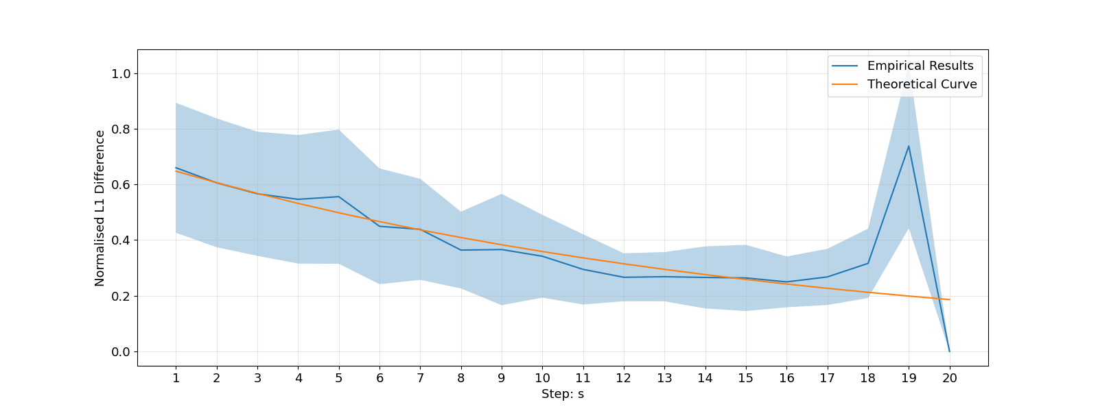
Figure 3: The L1-distance between a sample produced by an unperturbed flow and a flow where the attention map is perturbed at sample step s. We perturbed the pre-softmax attention map (in proportion to its norm) at step s for a 20-step DDIM solver. The results are scaled into the range [0,1] and then averaged over twenty random ImageNet labels as prompts; the shaded region includes one standard deviation. The orange line is an exponential of the form $k_{1}e^{-k_{2}s}$, tuned to best approximate the empirical results between steps 1 and 18 (inclusive). The correlation between these two curves in this range is 0.96.

4 Method

We begin this section by considering the limitations of our theoretically driven policy, HURRY. To remedy these limitations, we then rigorously search for policies close to HURRY with better efficacy.

What the Analysis Ignores. Although HURRY proves to be a reasonable initial policy, it ignores three important facts, which we will outline in turn. (1) Our dynamical model is imperfect: The exponential curve in Figure 3 deviates from the empirical results in the final two timesteps. We believe these anomalous boundary values deviate from our dynamical model because of a phase transition when particles move from intermediate states onto the image manifold itself. Nevertheless, this clearly demonstrates that our model doesn’t perfectly capture the DPM’s dynamics. (2) Attention map similarity is not constant: The maps from some steps in the sampling procedure are predictably closer to their temporally-adjacent neighbours (Figure 2). This variation isn’t factored into HURRY, which (implicitly) assumes uniform attention perturbations.

(3) HURRY assumes that step reuse is independent: Perhaps most consequentially, for $r>s$, reusing at step $s$ affects the model at step $r$. Thus, even if reuse at step $r$ is optimal for a single instance of reuse, it may no longer be wise after reuse at step $s$. Our perturbation analysis disregards these dependencies in order to make the analysis tractable. In order to remedy this, we will empirically explore local mutations of HURRY to determine whether they perform unexpectedly well due to some unforeseen dependencies. These mutations will also illuminate any other influences, such as factors (1) and (2), that cause deviations from HURRY’s ‘later is better’ reuse approach—producing a refined policy, which we refer to as PHAST.

Permuting HURRY. In the previous section, we developed HURRY as a strong but imperfect base policy. We translate this into the formal assumption that the local optimum closest to HURRY will also prove to be globally optimal. Here, a policy is defined as a local optimum if it outperforms every policy within a single bit-flip. We use the term ‘bit-flip’ to indicate the swapping of a reuse and a non-reuse step; this is the smallest mutation that preserves the number of reuse steps. Therefore, in this section, we search for a global optimum by iteratively testing whether our best observed policy (initialised as HURRY) is a local optimum.

To clarify our procedure (Algorithm 1), at each step of the search, we select the best policy we have observed so far and test whether this is a local optimum by evaluating all the policies that are one bit-flip away. If we reach a local optimum, then we terminate the search; otherwise, we continue. We refer to the result of this iterative local search as PHAST: Permuted Heuristic Attention STrategy. This name is derived from the fact that the composition of bit-flips produces an optimal permutation of HURRY.

Algorithm 1 Local search for an optimal reuse policy

$BestPolicy\leftarrow HURRY$

$Optima(i)\leftarrow 0\quad\forall i$

$Run\leftarrow 0$

repeat

     $Run\leftarrow Run+1$

     $Optima(Run)\leftarrow Optima(Run-1)$

     for $\pi\in BitFlippedSet(BestPolicy)$ do

         Sample $\boldsymbol{x}_{T}\text{ under reuse policy }\pi$

         if $PSNR\left(\boldsymbol{x}_{T}\right)>Optima(Run)+\varepsilon$ then

              $BestPolicy\leftarrow\pi$

              $Optima(Run)\leftarrow PSNR\left(\boldsymbol{\bar{x}}_{0}\right)$

         end if

     end for

until $Optima(Run)=Optima(Run-1)$

return $BestPolicy$

This search algorithm has a number of desirable properties. Firstly, it deterministically finds the closest (approximate) local optimum to HURRY, therefore results don’t need to be averaged over random seeds. Perhaps most importantly, it is very quick. For an N-step sampling procedure with R reuse steps, flipping all N(N-R) bits is only $\mathcal{O}(N^{2})$, in comparison to an exhaustive search, which is $\mathcal{O}(N^{R})$.

For example, in the case of a 20-step sampling procedure with ten reuse steps, this corresponds to one round of bit-flipping covering 100 policies, while an exhaustive search must cover 184,756 policies. Our search algorithm requires minimal rounds of bit-flipping to discover a local optimum, typically settling within one round of bit-flipping.

Why is the step-wise policy binary? Up to now, at each step, we have assumed that all layers either reuse or don’t. This ignores a natural axis for search that could bolster our performance, layer-wise reuse policies. However, there is an inherent trade-off, with step-wise policies and layer-wise policies vying for the same latency. To evaluate this trade-off, we compare layer-wise and step-wise policies of similar latencies. We already know what our step-wise policies look like, but what do the layer-wise policies look like?

Suppose we are given a step-wise reuse policy with a latency $L_{R}$ and a maximum latency budget of $L_{B}>L_{R}$. To produce a layer-wise refinement, we’re then given the option to turn off reuse for some layers in the model, within our latency budget, with the aim of maximising sample quality. Let $\boldsymbol{p}$ be a binary vector where $\boldsymbol{p}_{i}=0$ represents no changes to the existing step-wise policy at layer $i$. So $\boldsymbol{p}=\textbf{0}$ produces the initial step-wise policy with latency $L_{R}$.

If $\boldsymbol{p}_{i}=1$ then attention maps are always recalculated in layer $i$, regardless of the step-wise policy. This switches off reuse in layer $i$, increasing the latency and the sample quality. Additionally, let $\boldsymbol{l}_{i}$ denote the latency of layer $i$ and $\boldsymbol{d}_{i}$ denote the effect of re-calculating at layer $i$.

Intuitively, we wish to maximise $\textbf{p}\cdot\textbf{d}$ because $\textbf{d}_{i}$ denotes the (presumably positive) effect that re-calculating at layer $i$, as opposed to reusing, has on the sample. Thus, we must solve the following constrained optimisation problem:

$$\max\;\boldsymbol{p}\cdot\boldsymbol{d}\quad s.t.\quad\boldsymbol{p}\cdot\boldsymbol{l}<L_{B}-L_{R}.$$ (5)

In Figure 4 we compare policies that channel excess latency to reduce the number of reuse layers or reuse steps. We start with a base policy of HURRY with 10 reuse steps, and within a given latency budget, either switch off reuse for a subset of the layers or steps. We select the layers to turn off for a given latency budget by solving Equation 5.

To reduce the number of reuse steps, we simply evaluate HURRY with fewer (4-9) reuse steps. Comparing the two plots, we demonstrate that excess latency is best channelled towards minimising the number of reuse steps as opposed to refining the layer-wise strategy. This supports our focus in this paper on binary step-wise reuse policies that either switch reuse on or off for all layers in a given step.

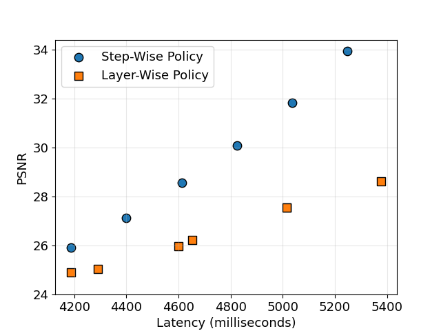
Figure 4: This figure compares the latency and PSNR of layer-wise (orange) and step-wise (blue) reuse policies. The PSNR is taken over 200 ImageNet labels as prompts.

5 Evaluation

So far, we have analysed and searched for optimal reuse policies; in this section, we must demonstrate that they actually work. We first compare our solutions with random (uninformed) reuse policies to demonstrate the efficacy of our search. Following this, we show that our reuse policies outperform step-reduced samplers.

Comparison With Random Policies. In Section 1, we motivated the need to shrewdly select reuse policies via Figure 1, which visually demonstrated the poor quality of random policies. To more formally compare HURRY and PHAST with random reuse policies, we evaluate their PSNR in Table 1. We find that they are both several standard deviations away from the average performance of random policies, justifying the importance of our analysis and policy search.

Solver	Stoch	HURRY	PHAST
DDIM	21.17$\pm$0.81	24.69	26.99

Table 1: A comparison of the performance (PSNR) of our 10-step reuse policies (HURRY and PHAST) with a collection of five stochastic (randomly generated) 10-step reuse policies. The mean $\pm$ standard deviation of the random policies is given.

Comparing Reuse to Step-Reduction. Given that our reuse policies outperform layer-wise and uninformed alternatives, we must now show that they outperform the canonical (increased step-size) approach to lowering latency. In Figures 4 and 5 we approximate the latency of these samplers by appropriately summing two components: (1) the latency of a full U-net call; and (2) the latency of a reuse U-net call. These latencies are estimated by calculating the share of total clock cycles used by each block of the U-net and scaling the total latency accordingly. We establish that a full U-net call has an approximate latency of 152ms, and reuse has an approximate latency of 47ms.

In Figure 5, we demonstrate that our proposed reuse strategies consistently outperform DDIM samplers of comparable latency. In this figure, the search for PHAST policies is run separately for each number of reuse steps. Figure 6 visually supports these results with samples from a cross-section of Figure 5, at a latency of $\sim$4000ms. This illustrates that the samples produced by our reuse policies are closer to those generated by a 20-step DDIM sampler than their step-reduced counterparts.

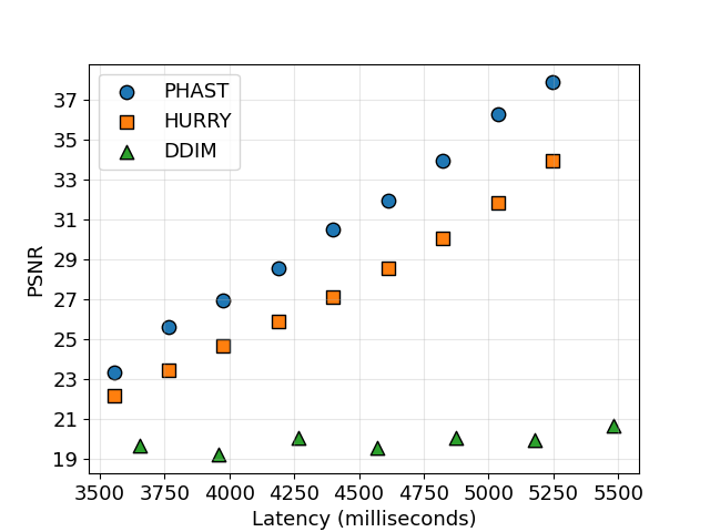
Figure 5: This figure compares the PSNR of PHAST, HURRY, and DDIM for comparable latencies. The PSNR is taken over 200 ImageNet labels as prompts.

Model	Method	DDIM			DPM++			Lat. (ms)†	Mem. (MiB)‡
		PSNR ($\uparrow$)	CLIP ($\uparrow$)	FID ($\downarrow$)	PSNR ($\uparrow$)	CLIP ($\uparrow$)	FID ($\downarrow$)
SD 1.5	Base(20)	ref.	0.2671	28.23	ref.	0.2673	27.11	4052	8091
	Base(13)	17.5	0.2681	28.22	17.16	0.2676	27.39	2664	8091
	PHAST	25.9	0.2667	29.18	23.02	0.2664	27.95	2937	12157
	PHAST${}_{\text{FP16}}$	25.95	0.2667	29.21	23.03	0.2664	27.95	3164	10141
SD 1.5 + CFG Dist.††	Base(20)	ref.	0.2611	31.71	ref.	0.2613	31.66	2090	7273
	Base(13)	17.68	0.2625	31.96	16.93	0.2619	31.16	1382	7273
	PHAST	28.63	0.2614	32.56	25.34	0.2612	32.66	1517	9093
	PHAST${}_{\text{FP16}}$	28.63	0.2614	32.57	25.34	0.2612	32.66	1623	8045
† avg. time needed to generate one image when running continuously for 5 minutes on an NVidia A40 (46GB) with maxed-out batch size (DPM++, full precision).
‡ total memory needed to generate one image (DPM++, full precision). $\quad{}^{\dagger\dagger}$ our reimplementation of ”stage one distillation” from [18].

Table 2: A comparison of our best policy (PHAST) with a base sampler (DPM-Solver [16] and DDIM) on the MS-COCO 2017 validation set, looking at PSNR, CLIP-Score, and FID. We evaluate our samplers on Stable Diffusion v1.5 (SD 1.5) and a low-latency distilled alternative that fuses the conditional and unconditional forward passes into one.

In Table 3 we present this same cross section at the $\sim$4000ms latency mark for three different samplers. The PHAST policies in this table were separately selected for every sampler. Up to a timestep rounding error, these policies are the same for all three samplers. This shows that our search generalises, which is perhaps unsurprising given that the U-net’s score function is unchanged between samplers.

Solver	Base	HURRY	PHAST
DDIM	19.22	24.69	26.99
DPM++	20.67	22.49	24.41
PLMS	18.32	21.96	23.62

Table 3: A comparison of HURRY and PHAST with a 13-step sampler (Base) for DDIM, DPM-Solver, and PLMS [13]. The reuse policies and base sampler each have a latency of $\sim$4000ms. PSNR is taken with a 20-step version of the base sampler.

Evaluation on MS-COCO. So far our evaluation has solely considered PSNR, in which we directly compare the samples produced by normal and reduced-latency approaches. In Section 3, we established a justification for this approach; however, in order to provide a holistic evaluation, in Table 2 we also assess the FID and CLIP-Score. Specifically, we compare the FID and CLIP-Score of PHAST with state-of-the-art samplers on the MS-COCO [12] validation dataset. These metrics directly (or implicitly) compare a sampler to an external dataset, providing a further lens into the performance of our reuse policies.

	English Setter	Laptop	Terrier	Macaw	Fire Truck	Taxi
DDIM(20)
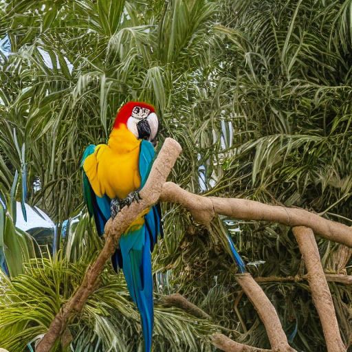
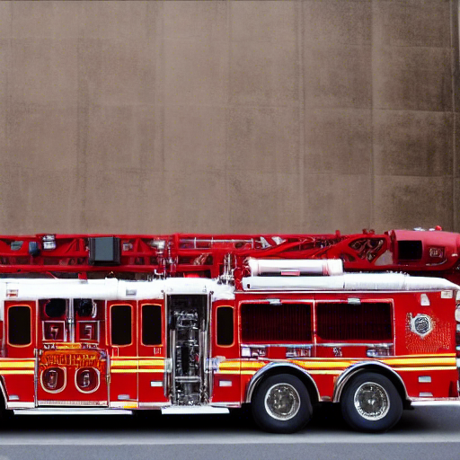
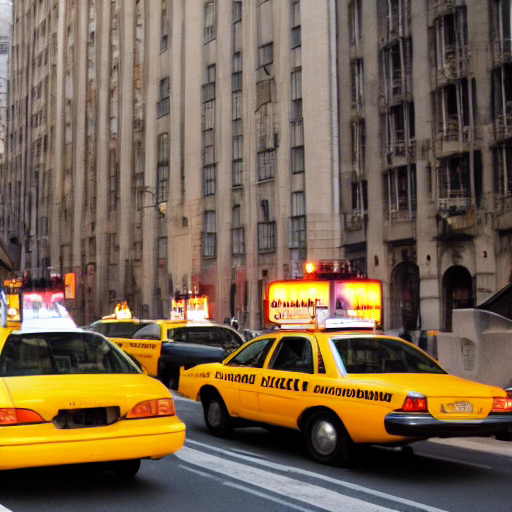
DDIM(13)
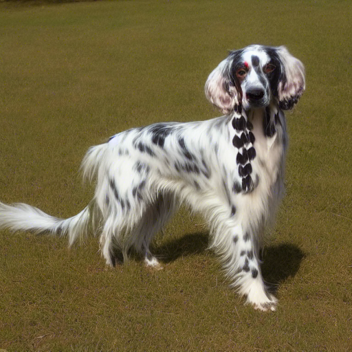
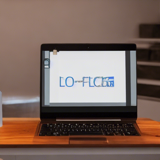
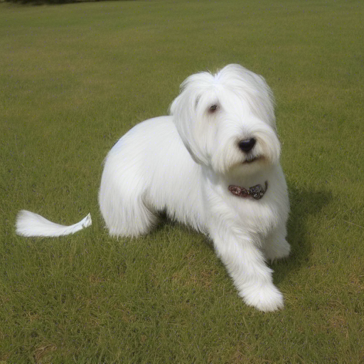
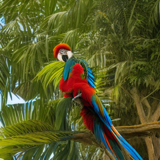
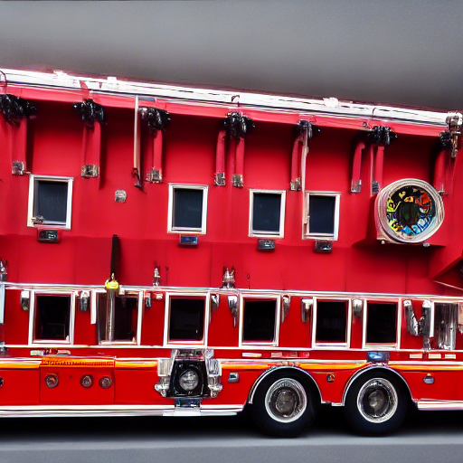
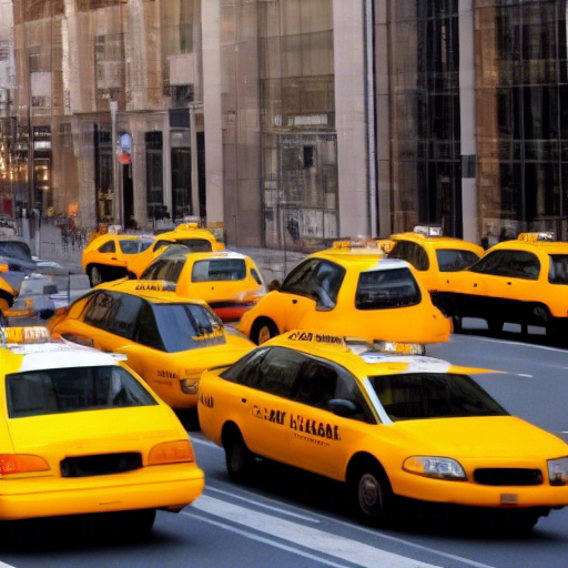
HURRY
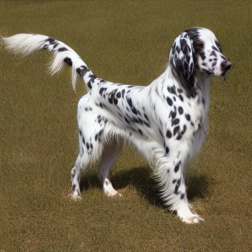
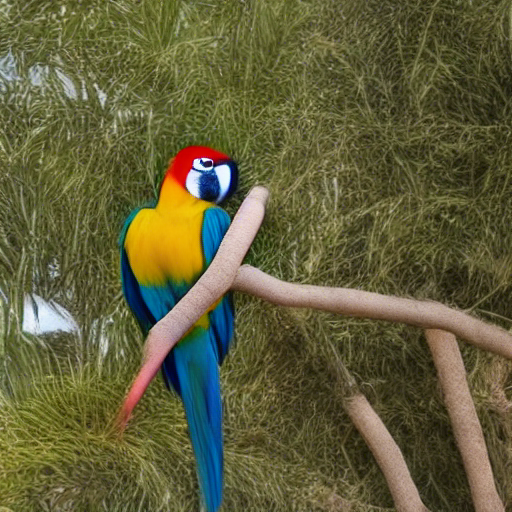
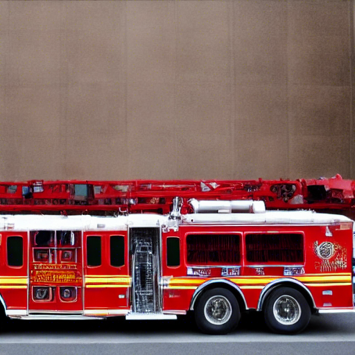
PHAST

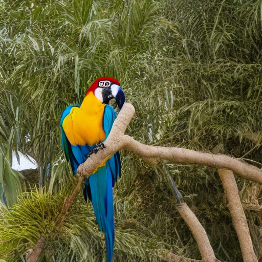
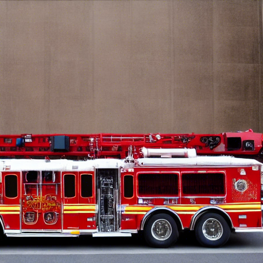
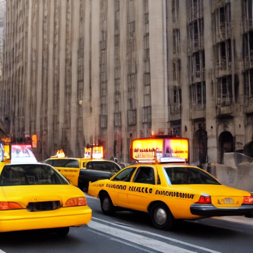
Figure 6: Visual comparison of the different sampling techniques for the prompts (column-wise): ‘English Setter’; ‘laptop, laptop computer’; ‘Sealyham terrier Sealyham’; ‘macaw’; ‘fire engine, fire truck’; ‘cab, hack, taxi, taxicab’. The samplers are (row-wise): 20-step DDIM; 13-step DDIM; HURRY with 10 reuse steps; PHAST with 10 reuse steps. The final three samplers all have a latency of $\sim$4000ms.

The CLIP-Score and FID of all three samplers are comparable (Table 2), with PHAST performing marginally worse in FID than the baseline samplers. This drop in performance suggests that reuse distorts samples away from a target distribution. However, as seen in Figure 6, these distortions are perhaps unnoticeable to the human eye. Notably, qualitative analysis in Figure 6 shows that DDIM with 13 steps can produce significantly distorted images — such as the firetruck which looks more like a building, the detached tail of the Terrier, or distorted body of the macaw. On the other hand, PHAST and HURRY, being designed to maximise fidelity w.r.t. the unperturbed flow, avoid such cases, at the expense of lost details and increased blurriness. This is validated quantitatively by significantly higher PSNR in Tab. 2.

Interestingly, the PSNR of PHAST is consistently larger for DDIM over DPM++. We attribute this difference to the more linear nature of DDIM, which, as we’ve previously discussed, should aid reuse. Along with evaluating PHAST for two different samplers, Table 2 also considers two different models. The top row is a vanilla version of Stable Diffusion, and the bottom row evaluates a model whose conditional and unconditional forward passes of the classifier-free guidance (CFG) are distilled into one, following [18].

We distilled the model using the MS-COCO 2013 training dataset with 4 A100 for 2-3 days only; we empirically validated that the model can produce decent images, see Supplementary Material (SM). We can see that even when a model has been additionally optimised, the same PHAST policy — searched for on vanilla stable diffusion — results in very similar behaviour, with very high fidelity (PSNR) and slight reduction in FID and CLIP. These results not only validate our method as a highly generalisable approach to accelerating DPMs (especially useful when remaining faithful to the baseline behaviour is of primary concern), it also shows complementarity of PHAST with other methods designed to optimise DPMs. For more experiments, see SM.

The Memory-Latency Trade-Off. The reductions in latency achieved by our reuse policies come at the expense of increased memory usage, which is required to cache the attention maps for reuse. Although our results in Tab. 2 show that speedup is not affected by this extra cost in the case of devices with high memory, the possibility to utilise reuse might be limited in memory-constrained system. To alleviate this, one possibility could be to opt for caching attention maps in reduced precision. In particular, we observe that storing attention maps in FP16 does not degrade results in any way while it allows us to halve the memory required to cache attention maps, see PHAST${}_{\text{FP16}}$ in Tab. 2.

We could reduce memory even further by considering, e.g., 8-bit quantisation — representatively, PHAST${}_{\text{INT8}}$ with our CFG-distilled model and the DPM++ solver achieves FID of 32.65 and PSNR of 25.35. However, we also notice that the overhead of performing quantisation becomes a bottleneck in this case, hurting latency; this is why we did not include full comparison. Having said that, we expect that this might be a feasible way forward for devices that operate on quantised tensors, since the cost of performing quantisation will be amortized in those cases. We leave further investigation into memory reduction for future work.

6 Conclusion

The main contributions of this work are reuse policies that reduce the latency of DPMs while retaining the step-size of the original sampler and the weights of the original model. Specifically, we produced two (increasingly refined) reuse policies that can be applied in a plug-and-play manner to improve latency with a minimal reduction in sample quality.

First, we discovered a positive (attention-adapted) Lyapunov exponent in the reverse diffusion process, suggesting a coarse step-wise policy. We then refined this policy by performing a local step-wise search. Finally, we showcased the strong performance of our reuse policies, generating samples closer to a baseline approach than step-reduction. Notably, our method offers a training-free way of accelerating DPMs that benefits from better guarantees about the impact of reducing computations w.r.t. the original flow — something that existing methods miss. We hope that future work can further investigate redundancies in the diffusion process that can be exploited to reduce the latency of DPMs.

Broader Impact. Our work reduces the latency of high-quality DPM image synthesis. While this may pose societal benefits, DPMs can also be used to produce biased or harmful content [1].

References

- Anderljung and Hazell [2023] Markus Anderljung and Julian Hazell. Protecting society from ai misuse: When are restrictions on capabilities warranted? arXiv preprint arXiv:2303.09377, 2023.
- Berthelot et al. [2023] David Berthelot, Arnaud Autef, Jierui Lin, Dian Ang Yap, Shuangfei Zhai, Siyuan Hu, Daniel Zheng, Walter Talbot, and Eric Gu. Tract: Denoising diffusion models with transitive closure time-distillation. arXiv preprint arXiv:2303.04248, 2023.
- Bhojanapalli et al. [2021] Srinadh Bhojanapalli, Ayan Chakrabarti, Andreas Veit, Michal Lukasik, Himanshu Jain, Frederick Liu, Yin-Wen Chang, and Sanjiv Kumar. Leveraging redundancy in attention with reuse transformers. arXiv preprint arXiv:2110.06821, 2021.
- Deng et al. [2009] Jia Deng, Wei Dong, Richard Socher, Li-Jia Li, Kai Li, and Li Fei-Fei. Imagenet: A large-scale hierarchical image database. In 2009 IEEE conference on computer vision and pattern recognition, pages 248–255. Ieee, 2009.
- Dhariwal and Nichol [2021] Prafulla Dhariwal and Alexander Nichol. Diffusion models beat gans on image synthesis. Advances in Neural Information Processing Systems, pages 8780–8794, 2021.
- Dockhorn et al. [2022] Tim Dockhorn, Arash Vahdat, and Karsten Kreis. Genie: Higher-order denoising diffusion solvers. Advances in Neural Information Processing Systems, pages 30150–30166, 2022.
- Gu et al. [2023] Jiatao Gu, Shuangfei Zhai, Yizhe Zhang, Lingjie Liu, and Josh Susskind. Boot: Data-free distillation of denoising diffusion models with bootstrapping. arXiv preprint arXiv:2306.05544, 2023.
- Kim et al. [2023] Bo-Kyeong Kim, Hyoung-Kyu Song, Thibault Castells, and Shinkook Choi. On architectural compression of text-to-image diffusion models. arXiv preprint arXiv:2305.15798, 2023.
- Kingma et al. [2021] Diederik Kingma, Tim Salimans, Ben Poole, and Jonathan Ho. Variational diffusion models. Advances in Neural Information Processing Systems, pages 21696–21707, 2021.
- Layek et al. [2015] GC Layek et al. An introduction to dynamical systems and chaos. Springer, 2015.
- Li et al. [2023] Yanyu Li, Huan Wang, Qing Jin, Ju Hu, Pavlo Chemerys, Yun Fu, Yanzhi Wang, Sergey Tulyakov, and Jian Ren. Snapfusion: Text-to-image diffusion model on mobile devices within two seconds. arXiv preprint arXiv:2306.00980, 2023.
- Lin et al. [2014] Tsung-Yi Lin, Michael Maire, Serge Belongie, James Hays, Pietro Perona, Deva Ramanan, Piotr Dollár, and C Lawrence Zitnick. Microsoft coco: Common objects in context. In Computer Vision–ECCV 2014: 13th European Conference, Zurich, Switzerland, September 6-12, 2014, Proceedings, Part V 13, pages 740–755. Springer, 2014.
- Liu et al. [2022] Luping Liu, Yi Ren, Zhijie Lin, and Zhou Zhao. Pseudo numerical methods for diffusion models on manifolds. arXiv preprint arXiv:2202.09778, 2022.
- Liu et al. [2023] Xingchao Liu, Xiwen Zhang, Jianzhu Ma, Jian Peng, and Qiang Liu. Instaflow: One step is enough for high-quality diffusion-based text-to-image generation. arXiv preprint arXiv:2309.06380, 2023.
- Lu et al. [2022a] Cheng Lu, Yuhao Zhou, Fan Bao, Jianfei Chen, Chongxuan Li, and Jun Zhu. Dpm-solver: A fast ode solver for diffusion probabilistic model sampling in around 10 steps. Advances in Neural Information Processing Systems, 35:5775–5787, 2022a.
- Lu et al. [2022b] Cheng Lu, Yuhao Zhou, Fan Bao, Jianfei Chen, Chongxuan Li, and Jun Zhu. Dpm-solver++: Fast solver for guided sampling of diffusion probabilistic models. arXiv preprint arXiv:2211.01095, 2022b.
- Luo [2022] Calvin Luo. Understanding diffusion models: A unified perspective. arXiv preprint arXiv:2208.11970, 2022.
- Meng et al. [2023] Chenlin Meng, Robin Rombach, Ruiqi Gao, Diederik Kingma, Stefano Ermon, Jonathan Ho, and Tim Salimans. On distillation of guided diffusion models. In Proceedings of the IEEE/CVF Conference on Computer Vision and Pattern Recognition, pages 14297–14306, 2023.
- Nichol et al. [2021] Alex Nichol, Prafulla Dhariwal, Aditya Ramesh, Pranav Shyam, Pamela Mishkin, Bob McGrew, Ilya Sutskever, and Mark Chen. Glide: Towards photorealistic image generation and editing with text-guided diffusion models. arXiv preprint arXiv:2112.10741, 2021.
- Platen [1999] Eckhard Platen. An introduction to numerical methods for stochastic differential equations. Acta numerica, pages 197–246, 1999.
- Ramesh et al. [2022] Aditya Ramesh, Prafulla Dhariwal, Alex Nichol, Casey Chu, and Mark Chen. Hierarchical text-conditional image generation with clip latents. arXiv preprint arXiv:2204.06125, 2022.
- Rombach et al. [2022] Robin Rombach, Andreas Blattmann, Dominik Lorenz, Patrick Esser, and Björn Ommer. High-resolution image synthesis with latent diffusion models. In Proceedings of the IEEE/CVF Conference on Computer Vision and Pattern Recognition, pages 10684–10695, 2022.
- Saharia et al. [2022] Chitwan Saharia, William Chan, Saurabh Saxena, Lala Li, Jay Whang, Emily L Denton, Kamyar Ghasemipour, Raphael Gontijo Lopes, Burcu Karagol Ayan, Tim Salimans, et al. Photorealistic text-to-image diffusion models with deep language understanding. Advances in Neural Information Processing Systems, pages 36479–36494, 2022.
- Salimans and Ho [2022] Tim Salimans and Jonathan Ho. Progressive distillation for fast sampling of diffusion models. arXiv preprint arXiv:2202.00512, 2022.
- Song et al. [2020a] Jiaming Song, Chenlin Meng, and Stefano Ermon. Denoising diffusion implicit models. arXiv preprint arXiv:2010.02502, 2020a.
- Song et al. [2020b] Yang Song, Jascha Sohl-Dickstein, Diederik P Kingma, Abhishek Kumar, Stefano Ermon, and Ben Poole. Score-based generative modeling through stochastic differential equations. arXiv preprint arXiv:2011.13456, 2020b.
- Song et al. [2023] Yang Song, Prafulla Dhariwal, Mark Chen, and Ilya Sutskever. Consistency models. 2023.
- Xu et al. [2023] Yilun Xu, Mingyang Deng, Xiang Cheng, Yonglong Tian, Ziming Liu, and Tommi Jaakkola. Restart sampling for improving generative processes. arXiv preprint arXiv:2306.14878, 2023.