Point canonical transformation (PCT) has been used to find out new exactly solvable potentials in the position-dependent mass (PDM) framework. We solve $1$-D Schrödinger equation in the PDM framework by considering two different fairly generic position-dependent masses $(i)M(x)=\lambda g^{\prime}(x)$ and $(ii)M(x)=c\left({g^{\prime}(x)}\right)^{\nu}$,  $\nu=\frac{2\eta}{2\eta+1},$ with $\eta=0,1,2\cdots$. In the first case, we find new exactly solvable potentials that depend on an integer parameter $m$, and the corresponding solutions are written in terms of $X_{m}$-Laguerre polynomials. In the latter case, we obtain a new one parameter $(\nu)$ family of isochronous solvable potentials whose bound states are written in terms of $X_{m}$-Laguerre polynomials. Further, we show that the new potentials are shape invariant by using the supersymmetric approach in the framework of PDM.

1 Introduction

In quantum mechanics, the Schrödinger equation for a few systems is solved exactly though the traditional means [1], the factorization methods of supersymmetric quantum mechanics (SUSY) [2, 3, 4, 5, 6, 7], Lie algebraic techniques [8, 9, 10], reduction approach (to a hypergeometric equation [11] or to a confluent Heun equation [12]), Nikiforov-Uvarov (NU) method [13, 14] etc. Searching for analytically solvable potentials, whose energy spectrum are completely known, constitute an important field to study the low dimensional structures e.g. quantum well, quantum dot [15], specially the linear and nonlinear optical properties of the same [16, 17, 18]. On the other hand, the scenario of non-constant mass particularly position-dependent mass (PDM), although initially pursued in condensed matter physics problems, has become an active area of research in many disciplines of physics. The significant advancement in crystallographic growth techniques that enable the manufacture of non-uniform semiconductor specimens with abrupt heterojunctions is what has drawn the attention to the PDM approach. This kind of spatial dependencies have provided useful insights into new classes of phenomena such as the transport proprieties in semiconductors [15, 19], compositionally graded crystals [20], quantum dots [21], liquid crystals [22], and extended systems governed by superintegrability [23, 24]. The concept of PDM is also used for generating the pseudo-potentials which have an essential computational advantage in quantum Monte Carlo method [25, 26]. On aside earlier studies on fundamental length scale (to remove divergences in field theories) show that any modification to the underlying space or to the canonical commutation relations (i.e Heisenberg uncertainty relation) [27, 28] can result to a Schrödinger equation with a position-dependent mass [29, 30]. To study these inhomogeneous materials we need to have an effective way to solve the PDM Schrödinger equation (PDMSE) which we will address in this article. Before going further it needs to be emphasized that in any scheme for the same leads to non-commutativity of the momentum and mass-operators and it results in an ordering ambiguity in the kinetic energy (KE) representation (see, e.g., [31, 32]). To avoid this we will use the Ben-Daniel and Duke model of PDMSE [33] for our study.

The bound state solutions of the Schrödinger equation are generally associated with some classical orthogonal polynomials such as Hermite polynomials, Laguerre polynomials, Legendre polynomials, etc. In 2009, new families of orthogonal polynomials connected to their classical counterparts were introduced and termed exceptional orthogonal polynomials (EOPs)[34, 35, 36]. These polynomials form an orthogonal and complete set of polynomials with a positive weight function even if their sequence starts with a degree $n\geq 1$. After this remarkable discovery, the quantum mechanical exploration of exactly solvable systems has been boosted, particularly those whose solutions are written in terms of EOPs. These are known as rational extensions of usual quantum systems. Over the past decade, these advancements have significantly expanded the list of exactly solvable potentials.[37, 38, 39, 40, 41, 42, 43, 44].

In this article, we consider the PCT approach to construct the new exactly solvable potentials in a PDM background. We study the two cases, in the first case, we consider $M(x)=\lambda g^{\prime}(x)$ which was also considered [45] to obtain the solution of PDMSE in terms of $X_{1}$-Laguerre polynomials. We find new exactly solvable potentials and the eigenstates associated with these potentials are written in terms of $Xm$-Laguerre EOPs. It is important to note that numerous research have already been done on the intriguing problem of how classical and quantum ”generalised harmonicity” relate to one another to which end we encounter with isochronous potentials [46, 47]. Stillinger and Stillinger [46] have suggested a two-parameter family of isochronous potentials, interpolating between the harmonic oscillator and the asymmetric parabolic well, while Dorignac has explored the quantum spectrum of the same which comes as equispaced [47]. In the second case, we propose a general form of $M(x)=c\left({g^{\prime}(x)}\right)^{\nu},\ \nu=\frac{2\eta}{2\eta+1},$ with $\eta=0,1,2\cdots$ and obtain a one-parameter family of isochronous potentials that are exactly solvable and asymmetric in nature. Solutions are constructed in terms of $X_{m}$-Laguerre EOPs. It is worth adding that a similar study has already been undertaken for different choices of $M(x)$[48, 45, 49]. Furthermore, by using the supersymmetric approach in quantum mechanics in the context of a PDEM framework, we show that these exactly solvable potentials are shape-invariant.

The organization of this paper is as follows: in section $2$ we briefly introduce the position-dependent mass Schrödinger equation and deformed algebra. In section $3$ we have generated two new exactly solvable potentials by using the point canonical transformation approach in the position-dependent effective mass background whose wavefunctions are written in terms of $X_{m}$ Laguerre orthogonal polynomials. In section $4$ we have shown that these new exactly solvable potentials are shape invariant via using SUSY in quantum mechanics in PDM background. Finally, in section $5$ we summarize the result.

2 PDM Schrödinger Equation and Deformed Algebra

To avoid the noncommutativity, we start with the von Roos prescription of the two-parameter formulation of an effective-mass kinetic energy (KE) operator [50], which has an inbuilt Hermiticity (which also yields different plausible special cases), reads as

$$\hat{T}=\frac{1}{4}[\mathcal{M}^{r}(x)p\mathcal{M}^{s}(x)p\mathcal{M}^{t}(x)+\mathcal{M}^{t}(x)p{\mathcal{M}}^{s}(x)p\mathcal{M}^{r}(x)]$$ (1)

where $r$, $s$ and $t$ constitute a set of ambiguity parameters which follow $r+s+t=-1$. Using the above $\hat{T}$, we can write the Hamiltonian for PDMSE as follows

$$H=\Big{[}\frac{1}{4}[\mathcal{M}^{r}(x)p\mathcal{M}^{s}(x)p\mathcal{M}^{t}(x)+\mathcal{M}^{t}(x)p\mathcal{M}^{s}(x)p\mathcal{M}^{r}(x)]+V(x)\Big{]},$$ (2)

where $V(x)$ is the external potential. Of the frequently used Hermitian Hamiltonians, a few possible choices of the ambiguity parameters, have been explored in the literature for that see [51] and references therein.

Adopting units such that $\hbar=2\mathcal{M}_{0}=1$ the PDMSE corresponding to the Hamiltonian in (2) can be projected as

$$\Big{[}-\frac{1}{2}\Big{(}M^{r}(x)\frac{d}{dx}M^{s}(x)\frac{d}{dx}M^{t}(x)+M^{t}(x)\frac{d}{dx}M^{s}(x)\frac{d}{dx}M^{r}(x)\Big{)}+V(x)\Big{]}\psi(x)=E\psi(x)$$ (3)

where $M(x)$ is defined by $\mathcal{M}(x)=\mathcal{M}_{0}M(x)$ and is dimensionless. On setting $M(x)=f^{-2}(x)$ and $\quad f(x)=1+\mathfrak{g}(x)$ [52], where $f(x)$ is some positive-definite function and $\mathfrak{g}(x)=0$ corresponds to the constant-mass case, equation (3) becomes

$$\Big{[}-\frac{1}{2}\Big{(}f^{r}(x)\frac{d}{dx}f^{s}(x)\frac{d}{dx}f^{t}(x)+f^{t}(x)\frac{d}{dx}f^{s}(x)\frac{d}{dx}f^{r}(x)\Big{)}+V(x)\Big{]}\psi(x)=E\psi(x)$$ (4)

with $r+s+t=2$. We can get rid of the ambiguity parameters $r$, $s$, $t$ (denoted collectively by a) in the kinetic energy term by transferring them to the effective potential energy of the variable-mass system. Then using the result

$$f^{r}\frac{d}{dx}f^{s}\frac{d}{dx}f^{t}+f^{t}\frac{d}{dx}f^{s}\frac{d}{dx}f^{r}=2\sqrt{f}\frac{d}{dx}f\frac{d}{dx}\sqrt{f}-(1-r-t)ff^{{}^{\prime\prime}}-2(\frac{1}{2}-r)(\frac{1}{2}-t)f^{{}^{\prime}2}$$ (5)

where the prime denotes derivative with respect to $x$ and the positive definiteness of $f$ is explicitly assumed, equation (4) acquires the form

$$H\psi(x)=\big{[}-\Big{(}\sqrt{f(x)}\frac{d}{dx}\sqrt{f(x)}\Big{)}^{2}+V_{eff}(x)\Big{]}\psi(x)=E\psi(x)$$ (6)

in which the effective potential

$$V_{eff}(x)=V(x)+\frac{1}{2}(1-r-t)f(x)f^{\prime\prime}(x)+(\frac{1}{2}-r)(\frac{1}{2}-t)f^{{}^{\prime}2}(x)$$ (7)

The PDMSE (6) may now be reinterpreted as the deformed Schrödinger equation as given by

$$H\psi(x)=\big{[}\pi^{2}+V_{eff}(x)\Big{]}\psi(x)=E\psi(x)$$ (8)

where the standard momentum operator $p=-i\frac{d}{dx}$ is now modified by the following deformed quantity defined by $\pi=-i\sqrt{f(x)}\frac{d}{dx}\sqrt{f(x)}$ and we thus observe that with respect to $\pi$ the conventional commutation relation $[x,p]=i~{}\hbar$ is modified to $[x,\pi]=i~{}\hbar f(x)$ where $f(x)$ acts as a deforming function[27, 52, 53]. This type of deformation also has been extensively studied in different areas of physics such as in statistical physics (knowing as $q-$deformed algebra)[54, 55], in optics [56, 57] as well as black hole physics [58, 59]. In the next section, we will use the PCT and EOPs to obtain a class of exactly solvable potentials and their eigen spectrum.

3 Generation of new potential by PCT approach

Following the procedure outlined in the previous section the PDMSE in Eq. (3) can be written as

$$H\psi(x)=\Big{[}-\frac{d}{dx}\frac{1}{M(x)}\frac{d}{dx}+V_{eff}\Big{]}\psi(x)=E\psi(x)$$ (9)

where the effective potential is

$$V_{eff}(x)=V(x)+\frac{s+1}{2}\frac{M^{\prime\prime}}{M^{2}}-[r(r+s+1)+s+1]\frac{{M^{\prime}}^{2}}{M^{3}}$$ (10)

$V(x)$ is the applied potential in the system. We will follow the choice of BenDaniel and Duke [33], i.e. $r=t=0$ and $s=-1$ for which the effective and applied potentials become identical. We use the solution $\psi(x)$ in the form given by [52, 49, 45]

$$\psi(x)=f(x)F(g(x))$$ (11)

where $F(g(x))$ satisfies second order differential equation

$$\frac{d^{2}F}{dg^{2}}+Q(g)\frac{dF}{dg}+R(g)F=0$$ (12)

Now substituting this $\psi(x)$ in Eq. (9) we get

$$\frac{d^{2}F}{{dg}^{2}}+\left(\frac{g^{\prime\prime}}{{g^{\prime}}^{2}}+\frac{2f^{\prime}}{fg^{\prime}}-\frac{M^{\prime}}{Mg^{\prime}}\right)\frac{dF}{dg}+\Big{(}\frac{f^{\prime\prime}}{f{g^{\prime}}^{2}}-\frac{M^{\prime}f^{\prime}}{Mf{g^{\prime}}^{2}}+(E-V_{eff})\frac{M}{{g^{\prime}}^{2}}\Big{)}F=0$$ (13)

On comparison we get

$$Q(g(x))=\Big{(}\frac{g^{\prime\prime}}{{g^{\prime}}^{2}}+\frac{2f^{\prime}}{fg^{\prime}}-\frac{M^{\prime}}{Mg^{\prime}}\Big{)}$$ (14)

$$R(g(x))=\left(\frac{f^{\prime\prime}}{f{g^{\prime}}^{2}}-\frac{M^{\prime}f^{\prime}}{Mf{g^{\prime}}^{2}}+(E-V_{eff})\frac{M}{{g^{\prime}}^{2}}\right)$$ (15)

Eq. (14) admits the solution [49]

$$f(x)\propto\sqrt{\frac{M}{g^{\prime}}}e^{\frac{1}{2}\int^{g(x)}Q(t)dt}$$ (16)

Putting it in (15) we get

$$E-V_{eff}=\frac{g^{\prime\prime\prime}}{2Mg^{\prime}}-\frac{3}{4M}\left(\frac{g^{\prime\prime}}{g^{\prime}}\right)^{2}+\frac{{g^{\prime}}^{2}}{M}\left(R-\frac{1}{2}\frac{dQ}{dg}-\frac{Q^{2}}{4}\right)-\frac{M^{\prime\prime}}{2M^{2}}+\frac{3{M^{\prime}}^{2}}{4M^{3}}$$ (17)

To ensure the presence of an energy-like term on the right-hand side of the above equation, which will compensate for the term $E$ on its left-hand side, we can introduce a suitable relation between $M(x)$ and $g(x)$. This will give rise to an effective potential $V_{eff}(x)$ and the solution of the corresponding Schrödinger equation will be well-behaved. Three different choices of $M(x)\propto\left({g^{\prime}(x)}\right)^{\mu}$ with $\mu=-1,1,2$ have been used extensively in various applications of the PCT approach in the PDM context[60, 48]. In this article, we consider a new type of position-dependent mass

$$M(x)=c\left({g^{\prime}(x)}\right)^{\nu}$$ (18)

where $c$ is a proportionality constant, $\nu={\frac{2\,\eta}{2\,\eta+1}}$ and $\eta=0,1,2\cdots$ along with $M(x)=\lambda g^{\prime}(x)$

3.1 Case 1

For choice of $M(x)=\lambda g^{\prime}(x)$, Eq.(17) becomes

$$E-V_{eff}=\frac{g^{\prime}}{\lambda}\Big{(}R-\frac{1}{2}\frac{dQ}{dg}-\frac{Q^{2}}{4}\Big{)}.$$ (19)

We further consider the differential equation for $X_{m}$-Laguerre polynomials and compare it with equation (12) to get

$$\begin{gathered}Q=\frac{1}{g}\left((\alpha+1-g)-2g\frac{L_{m-1}^{\alpha}(-g)}{L_{m}^{\alpha-1}(-g)}\right),\quad\text{and }R=\frac{1}{g}\left(n-2\alpha\frac{L_{m-1}^{\alpha}(-g)}{L_{m}^{\alpha-1}(-g)}\right).\end{gathered}$$ (20)

where $F(g)\propto\hat{L}_{n,m}^{(\alpha)}(g)$.
For these values of $Q(g(x))$ and $R(g(x))$ equation (19) reads

$$E-V_{eff} =\frac{g^{\prime}}{\lambda g}\left(n-\left(m-\frac{1}{2}\right)+\frac{\alpha}{2}+\frac{m}{\alpha}\right)-\frac{g^{\prime}}{4\lambda}-\frac{g^{\prime}}{4g^{2}\lambda}\left(\alpha^{2}-1\right)-\frac{2g^{\prime}{L_{m}^{\alpha}(-g)}^{2}}{\lambda\left({L_{m}^{\alpha-1}(-g)}\right)^{2}}$$

$$\quad+\frac{g^{\prime}{L_{m-2}^{\alpha+1}(-g)}}{\lambda\left({L_{m}^{\alpha-1}(-g)}\right)}-\frac{g^{\prime}{L_{m-1}^{\alpha}(-g)}}{\lambda\left({L_{m}^{\alpha-1}(-g)}\right)}-\frac{g^{\prime}{L_{m-1}^{\alpha+1}(-g)}}{\alpha\lambda\left({L_{m}^{\alpha-1}(-g)}\right)}+\frac{g^{\prime}{L_{m-1}^{\alpha+1}(-g)}}{\lambda\left({L_{m}^{\alpha-1}(-g)}\right)}$$ (21)

We observe that choice $\frac{g^{\prime}}{\lambda g}=C$ will provide a constant term on the right-hand side to compensate for the energy term on the left-hand side. To get increasing eigenvalues for successive n-values, $C$ must be restricted to positive. The solution of the choice $\frac{g^{\prime}}{\lambda g}=C$ leads

$$g(x)=e^{-bx}~{}~{}\text{and}~{}~{}M(x)=e^{-bx},~{}~{}~{}~{}~{}-\infty<x<\infty$$ (22)

where we have considered $C=b^{2}$ and $C\lambda=-b,~{}b>0$.
Substituting Eq.(22) in (3.1) we obtain the effective potential and energy eigenvalues

$$V_{eff} =\frac{b^{2}}{4}\left(e^{bx}\left(\alpha^{2}-1\right)+e^{-bx}\right)+b^{2}\Bigg{(}\frac{2(L_{m-1}^{\alpha}(-e^{-bx}))^{2}}{\left({L_{m}^{\alpha-1}(-e^{-bx})}\right)^{2}}-\frac{{L_{m-2}^{\alpha+1}(-e^{-bx})}}{{L_{m}^{\alpha-1}(-e^{-bx})}}$$

$$\quad+\frac{{L_{m-1}^{\alpha+1}(-e^{-bx})}}{\alpha{L_{m}^{\alpha-1}(-e^{-bx})}}+\frac{{L_{m-1}^{\alpha}(-e^{-bx})}}{{L_{m}^{\alpha-1}(-e^{-bx})}}-\frac{{L_{m-1}^{\alpha+1}(-e^{-bx})}}{{L_{m}^{\alpha-1}(-e^{-bx})}}\Bigg{)}e^{-bx}+V^{I}_{c}$$ (23)

$$E_{n}^{m}=b^{2}\left(n+\frac{\alpha+1}{2}+\frac{m}{\alpha}\right)+V^{I}_{c},~{}~{}~{}n=0,1,2,...$$ (24)

where $V_{c}^{I}$ is an arbitrary constant. The eigenfunctions are obtained using Eqs.(11) and (16)

$$\psi_{n}^{m}(x)=\mathcal{N}\frac{\exp{[-\frac{1}{2}((\alpha+1)bx+e^{-bx})]}}{L_{m}^{\alpha-1}(-e^{-bx})}\hat{L}_{n+m,m}^{\alpha}(e^{-bx})~{}~{}~{}n=0,1,2,...$$ (25)

where $\mathcal{N}$ is the normalization constant given by

$$\mathcal{N}=\left(\frac{b~{}n!}{(n+m+\alpha)\Gamma(n+\alpha)}\right)^{\frac{1}{2}}$$

We would like to point out that $m=1$ case was done in [45] our general result for $X_{m}$ case reproduces the result of [45] as

$$V_{eff}=\frac{b^{2}}{4}\left(e^{bx}(\alpha^{2}-1)+e^{-bx}+\frac{4}{\alpha(1+\alpha e^{bx})}+\frac{8}{(1+\alpha e^{bx})^{2}}\right)+V^{I}_{c}$$ (26)

$$E_{n}^{1}=b^{2}\left(n+\frac{\alpha+1}{2}+\frac{1}{\alpha}\right)+V^{I}_{c},~{}~{}~{}n=0,1,2,...$$ (27)

$$\psi_{n}^{1}(x)=\mathcal{N}\frac{\exp{[-\frac{1}{2}((\alpha+1)bx+e^{-bx})]}}{\alpha+e^{-bx}}\hat{L}_{n+1}^{\alpha}(e^{-bx})~{}~{}~{}n=0,1,2,...$$ (28)

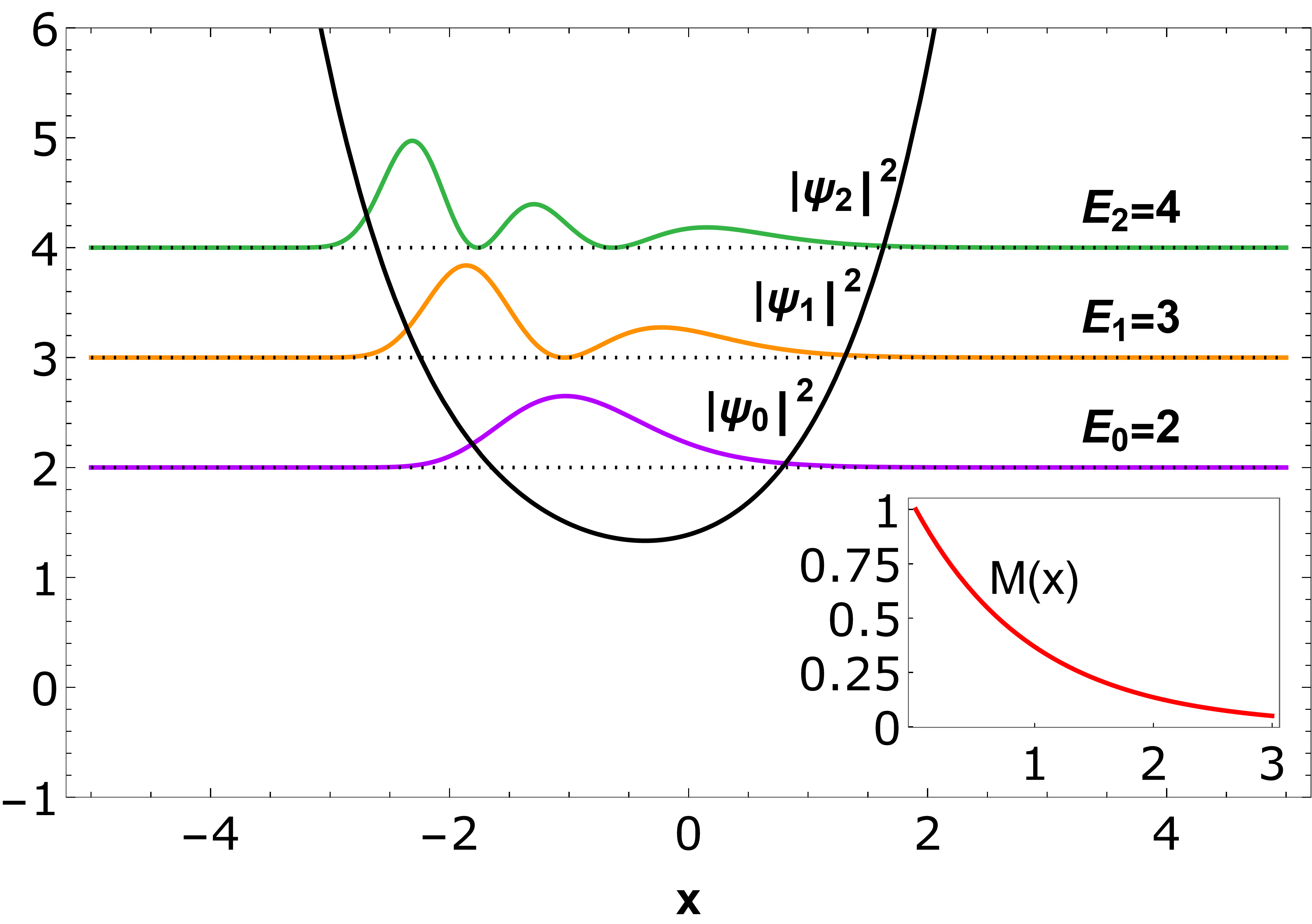
(a) $m=1$

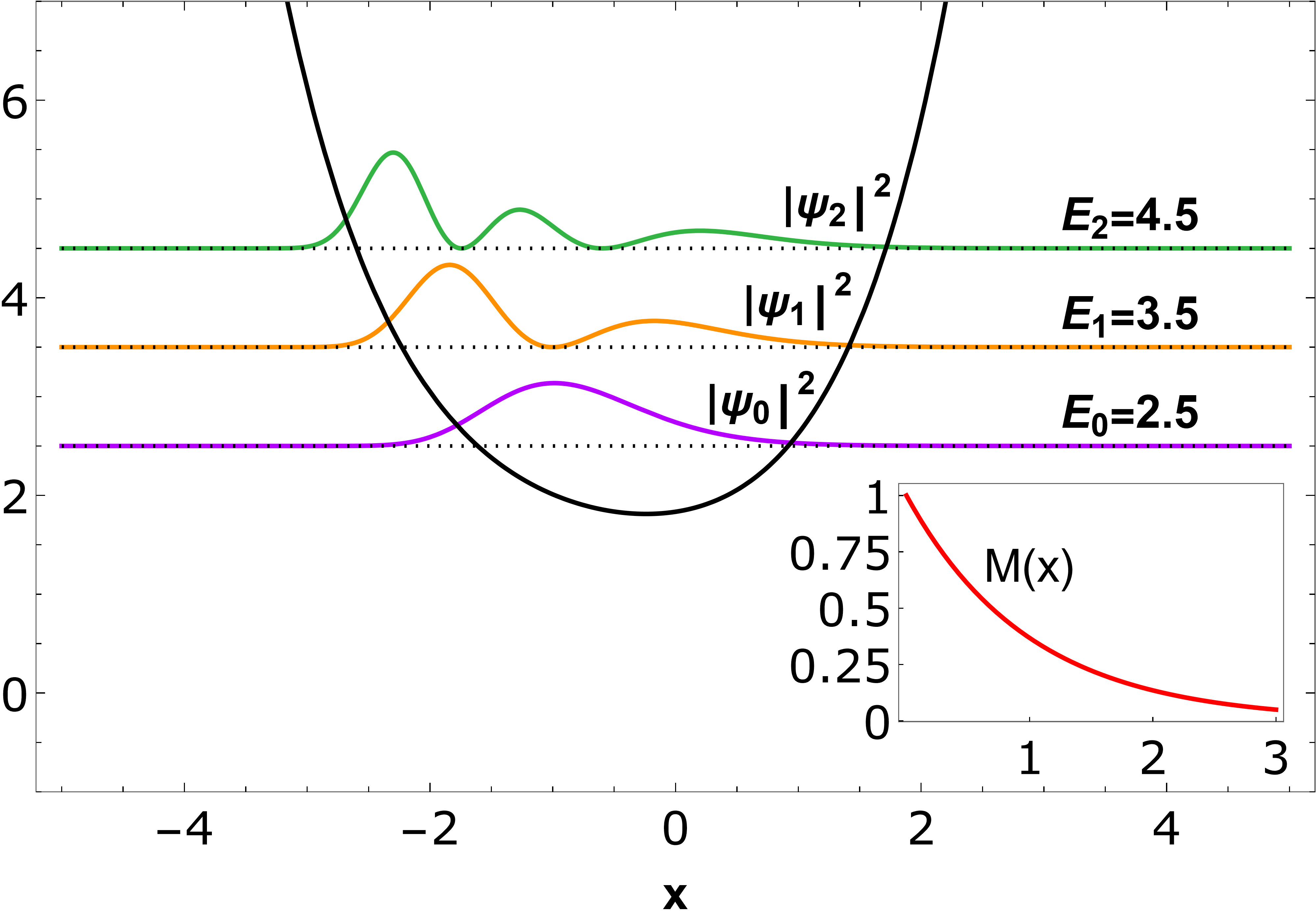
(b) $m=2$

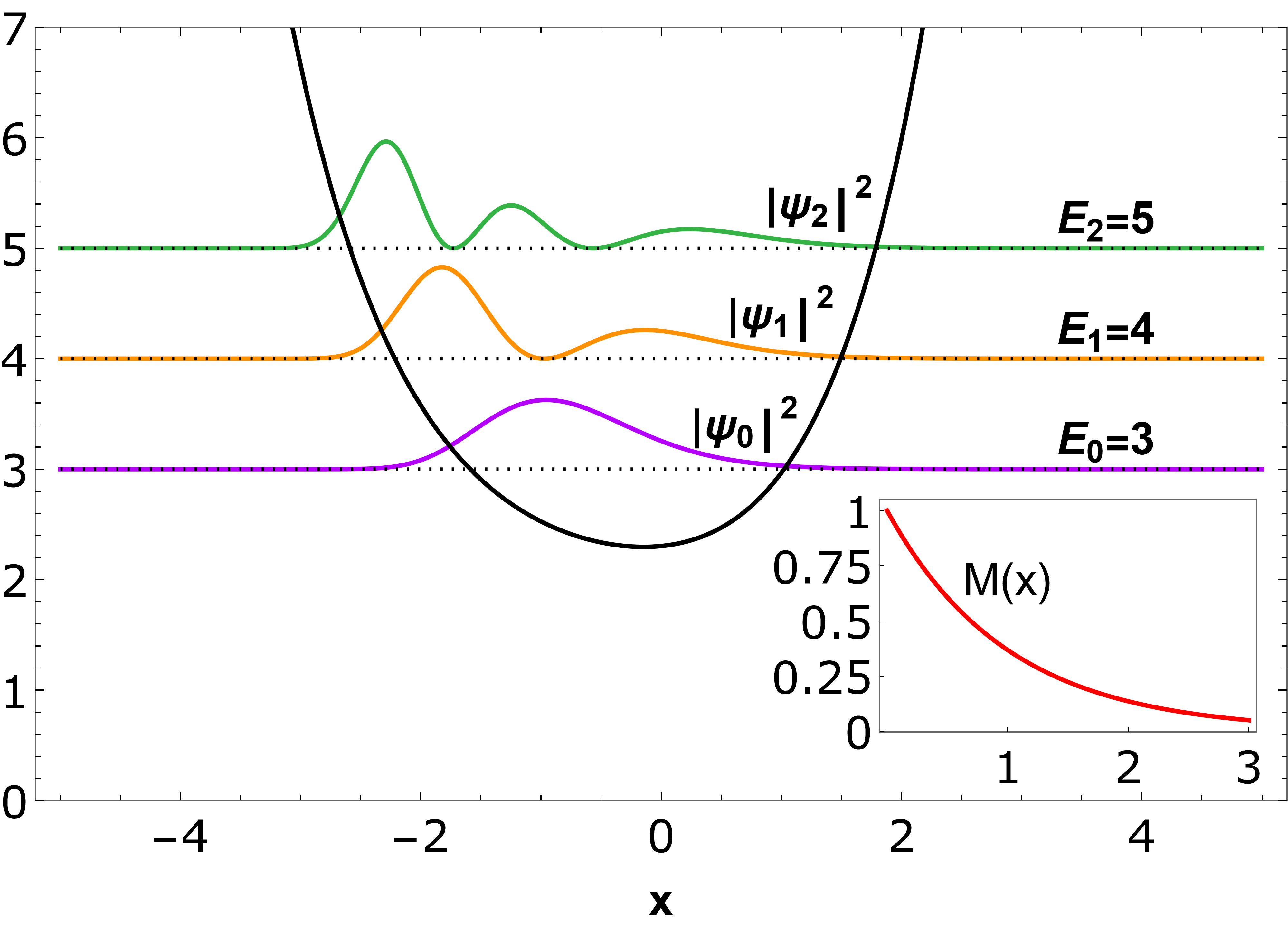
(c) $m=3$

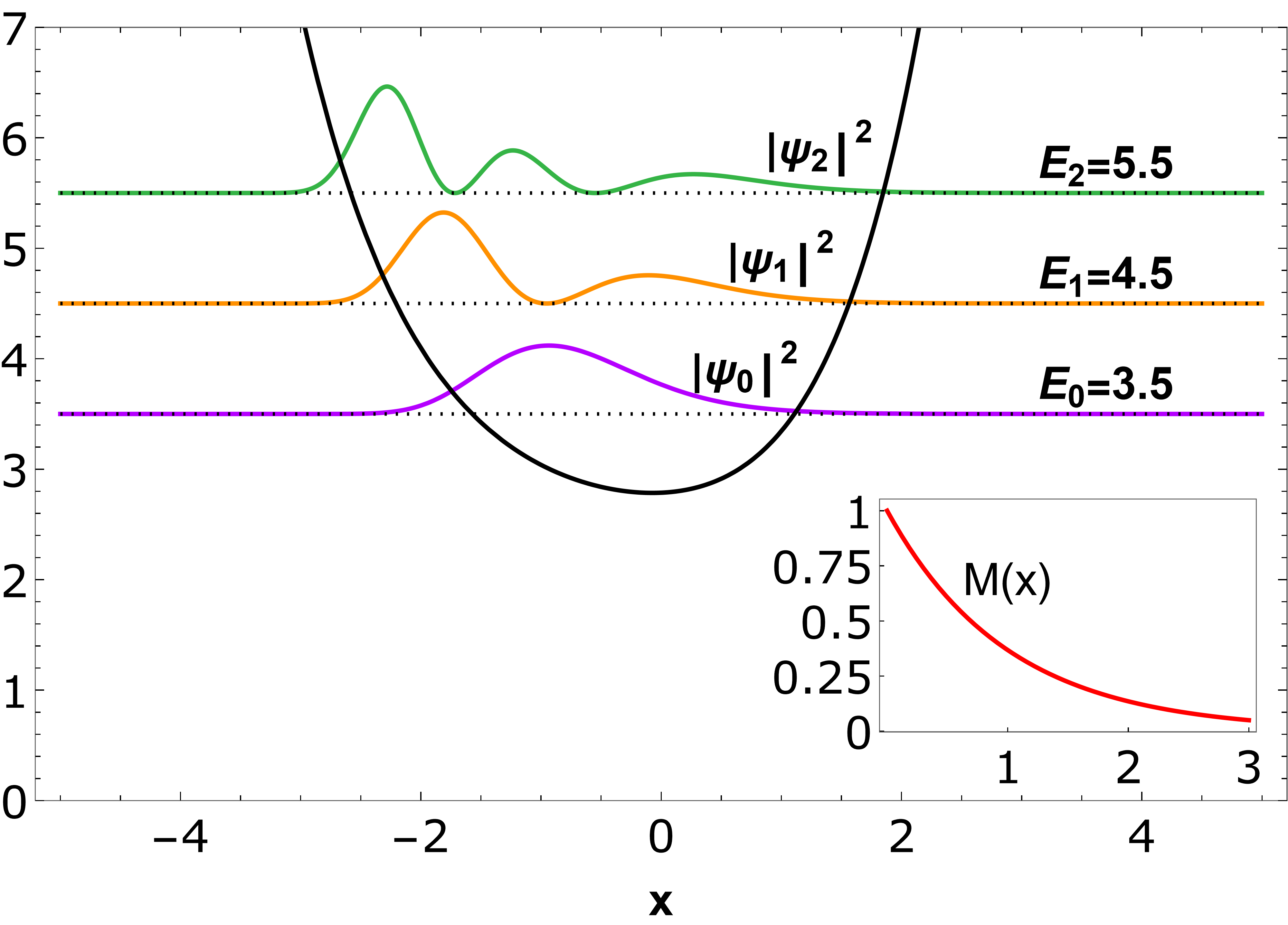
(d) $m=4$

Figure 1: Plot of the potential $V_{eff}$ given in Eq. (3.1) for different $m$ values, square of first three bound state wavefunctions ${|\psi_{0}|}^{2}$ (purple line), ${|\psi_{1}|}^{2}$ (orange line), ${|\psi_{2}|}^{2}$ (green line) corresponding to different $m$ values, for mass function $M(x)$ (red line) given in Eq. (22). We have consider here $b=1$, $\alpha=2$

3.2 Case 2

In this case, we consider a new type of position-dependent mass $M(x)=c\left({g^{\prime}(x)}\right)^{\nu},\nu={\frac{2\,\eta}{2\,\eta+1}}$ and $\eta=0,1,2\cdots$. For this choice Eq. (17) becomes

$$E-V_{eff} =\frac{g^{\prime\prime\prime}}{2c{g^{\prime}}^{(\nu+1)}}-\frac{3{g^{\prime\prime}}^{2}}{4c{g^{\prime}}^{(\nu+2)}}+\frac{1}{c{g^{\prime}}^{(\nu-2)}}\Big{(}R-\frac{1}{2}\frac{dQ}{dg}-\frac{Q^{2}}{4}\Big{)}$$

$$\quad-\frac{(\nu^{2}-\nu){g^{\prime\prime}}^{2}}{2c{g^{\prime}}^{(\nu+2)}}-\frac{\nu g^{\prime\prime\prime}}{2c{g^{\prime}}^{(\nu+1)}}+\frac{3\nu^{2}{g^{\prime\prime}}^{2}}{4c{g^{\prime}}^{(\nu+2)}}$$ (29)

We further consider the differential equation for $X_{m}$-Laguerre polynomials with equation (12) to get

$$\begin{gathered}Q=\frac{1}{g}\left((\alpha+1-g)-2g\frac{L_{m-1}^{\alpha}(-g)}{L_{m}^{\alpha-1}(-g)}\right),\quad\text{and }R=\frac{1}{g}\left(n-2\alpha\frac{L_{m-1}^{\alpha}(-g)}{L_{m}^{\alpha-1}(-g)}\right).\end{gathered}$$ (30)

where $F(g)\propto\hat{L}_{n,m}^{(\alpha)}(g)$.
For these values of $Q(g(x))$ and $R(g(x))$ equation (3.2) becomes

$$E-V_{eff} =\frac{{g^{\prime}}^{(2-\nu)}}{gc}\left(n-\left(m-\frac{1}{2}\right)+\frac{\alpha}{2}+\frac{m}{\alpha}\right)-\frac{{g^{\prime}}^{(2-\nu)}}{4c}-\frac{{g^{\prime}}^{(2-\nu)}}{4g^{2}c}\left(\alpha^{2}-1\right)-\frac{2{g^{\prime}}^{(2-\nu)}{L_{m}^{\alpha}(-g)}^{2}}{c\left({L_{m}^{\alpha-1}(-g)}\right)^{2}}$$

$$\quad+\frac{{g^{\prime}}^{(2-\nu)}{L_{m-2}^{\alpha+1}(-g)}}{c\left({L_{m}^{\alpha-1}(-g)}\right)}-\frac{{g^{\prime}}^{(2-\nu)}{L_{m-1}^{\alpha}(-g)}}{c\left({L_{m}^{\alpha-1}(-g)}\right)}-\frac{{g^{\prime}}^{(2-\nu)}{L_{m-1}^{\alpha+1}(-g)}}{\alpha c\left({L_{m}^{\alpha-1}(-g)}\right)}+\frac{{g^{\prime}}^{(2-\nu)}{L_{m-1}^{\alpha+1}(-g)}}{c\left({L_{m}^{\alpha-1}(-g)}\right)}$$

$$\quad-\frac{({\nu}^{2}-\nu){g^{\prime\prime}}^{2}}{2c{g^{\prime}}^{(\nu+2)}}-\frac{\nu g^{\prime\prime\prime}}{2c{g^{\prime}}^{(\nu+1)}}+\frac{3\nu^{2}{g^{\prime\prime}}^{2}}{4c{g^{\prime}}^{(\nu+2)}}+\frac{g^{\prime\prime\prime}}{2c{g^{\prime}}^{(\nu+1)}}-\frac{3{g^{\prime\prime}}^{2}}{4c{g^{\prime}}^{(\nu+2)}}$$ (31)

By following a similar approach as in the case $1$, we observe that the choice ${g^{\prime}}^{(2-\nu)}=\kappa\,c\,g$, where $\kappa$ is a constant, will provide a constant term on the right-hand side of the equation, corresponding to the energy term $E$ on the left-hand side. To get increasing eigenvalues for successive $n$ values, it is necessary to restrict the constant $\kappa$ to positive values.The solution of mentioned first order differential equation ${g^{\prime}}^{(2-\nu)}=\kappa\,c\,g$ reads $g(x)=x^{\frac{2-\nu}{1-\nu}}$, which generate $M(x)={\left(\frac{2-\nu}{1-\nu}\right)}^{2}x^{\frac{\nu}{1-\nu}}$. For simplicity we may take $\kappa\,c={(\frac{2-\nu}{1-\nu})}^{2}$ such that $\kappa=1$ and $c={(\frac{2-\nu}{1-\nu})}^{2}$. Substituting these values in Eq.(3.2) we obtain the effective potential and energy eigenvalues as

$$V_{eff} =\frac{1}{4}\left(x^{\frac{\nu-2}{1-\nu}}\left(\alpha^{2}-1\right)+x^{\frac{2-\nu}{1-\nu}}\right)+\Bigg{(}\frac{2(L_{m-1}^{\alpha}(-x^{\frac{2-\nu}{1-\nu}}))^{2}}{({L_{m}^{\alpha-1}(-x^{\frac{2-\nu}{1-\nu}})})^{2}}-\frac{{L_{m-2}^{\alpha+1}(-x^{\frac{2-\nu}{1-\nu}})}}{{L_{m}^{\alpha-1}(-x^{\frac{2-\nu}{1-\nu}})}}+\frac{{L_{m-1}^{\alpha+1}(-x^{\frac{2-\nu}{1-\nu}})}}{\alpha{L_{m}^{\alpha-1}(-x^{\frac{2-\nu}{1-\nu}})}}$$

$$\quad+\frac{{L_{m-1}^{\alpha}(-x^{\frac{2-\nu}{1-\nu}})}}{{L_{m}^{\alpha-1}(-x^{\frac{2-\nu}{1-\nu}})}}-\frac{{L_{m-1}^{\alpha+1}(-x^{\frac{2-\nu}{1-\nu}})}}{{L_{m}^{\alpha-1}(-x^{\frac{2-\nu}{1-\nu}})}}\Bigg{)}x^{\frac{2-\nu}{1-\nu}}+\frac{\left(1-\nu\right)\left(3-\nu\right)}{4{\left(2-\nu\right)}^{2}}x^{\frac{\nu-2}{1-\nu}}+V^{II}_{c}$$ (32)

$$E_{n}^{m}=\left(n+\frac{\alpha+1}{2}+\frac{m}{\alpha}\right)+V^{II}_{c},~{}~{}~{}n=0,1,2,...$$ (33)

where, $V^{II}_{c}$ is arbitrary constant.The eigenfunctions are obtained using Eqs.(11) and (16)

$$\psi_{n}^{m}(x)=\mathcal{N}\frac{\exp\left(\frac{-x^{\frac{2-\nu}{1-\nu}}}{2}\right)}{x^{\frac{1}{2}}\left(L_{m}^{\alpha-1}(-x^{\frac{2-\nu}{1-\nu}})\right)}x^{\frac{(2-\nu)(1+\alpha)}{2(1-\nu)}}\hat{L}_{n+m,m}^{\alpha}(x^{\frac{2-\nu}{1-\nu}}),~{}~{}~{}n=0,1,2,...$$ (34)

where $\mathcal{N}$ is the normalization constant and is given by

$$\mathcal{N}=\left(\frac{n!}{(n+m+\alpha)\Gamma(n+\alpha)}\right)^{\frac{1}{2}}$$

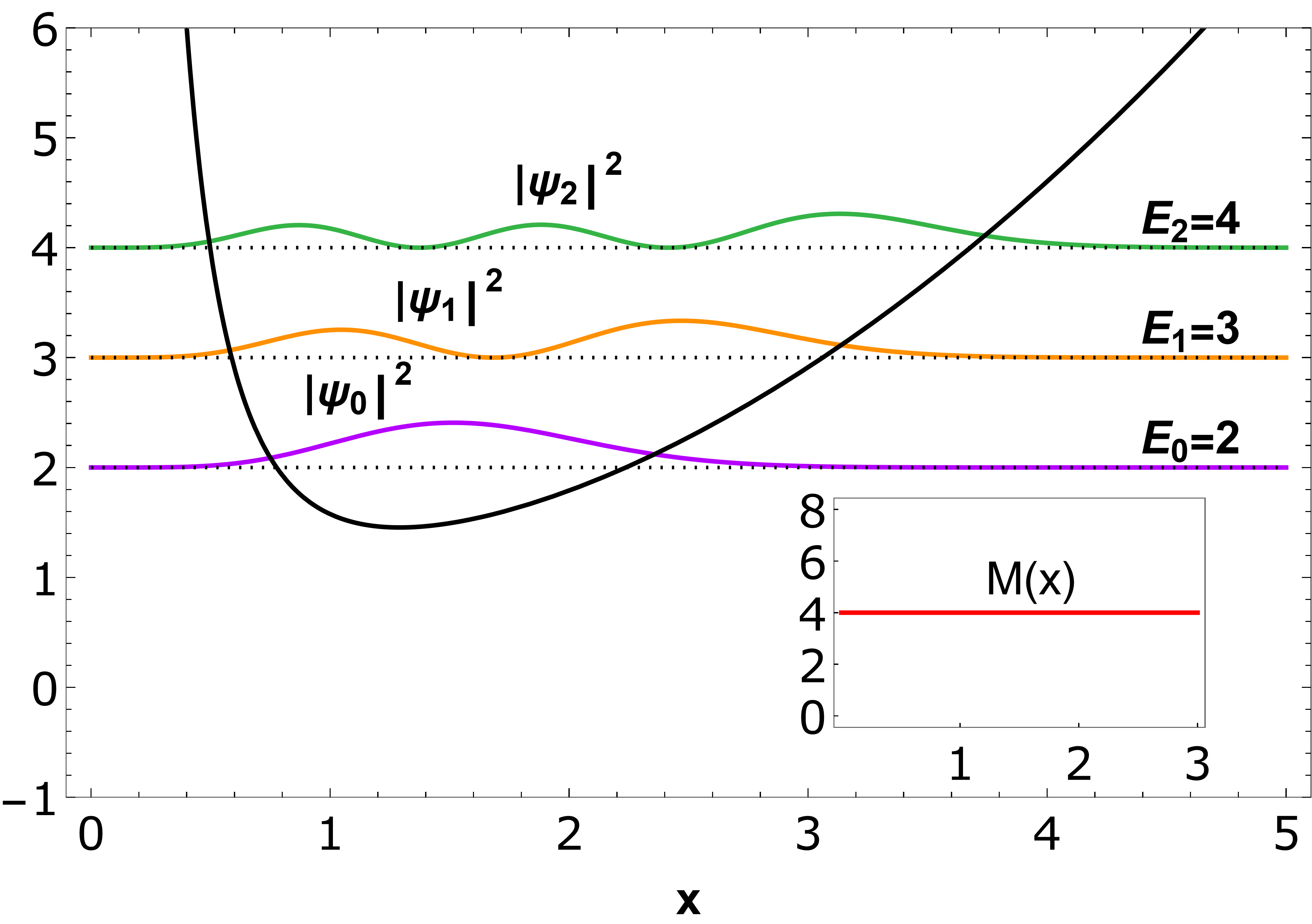
(a) $m=1,\nu=0$

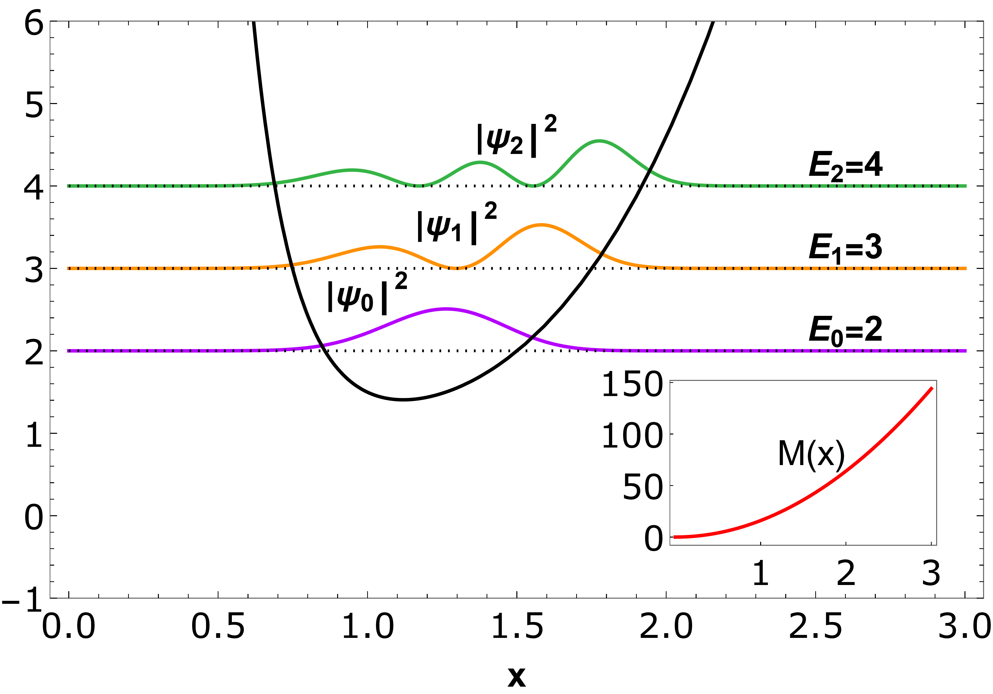
(b) $m=1,\nu=\frac{2}{3}$

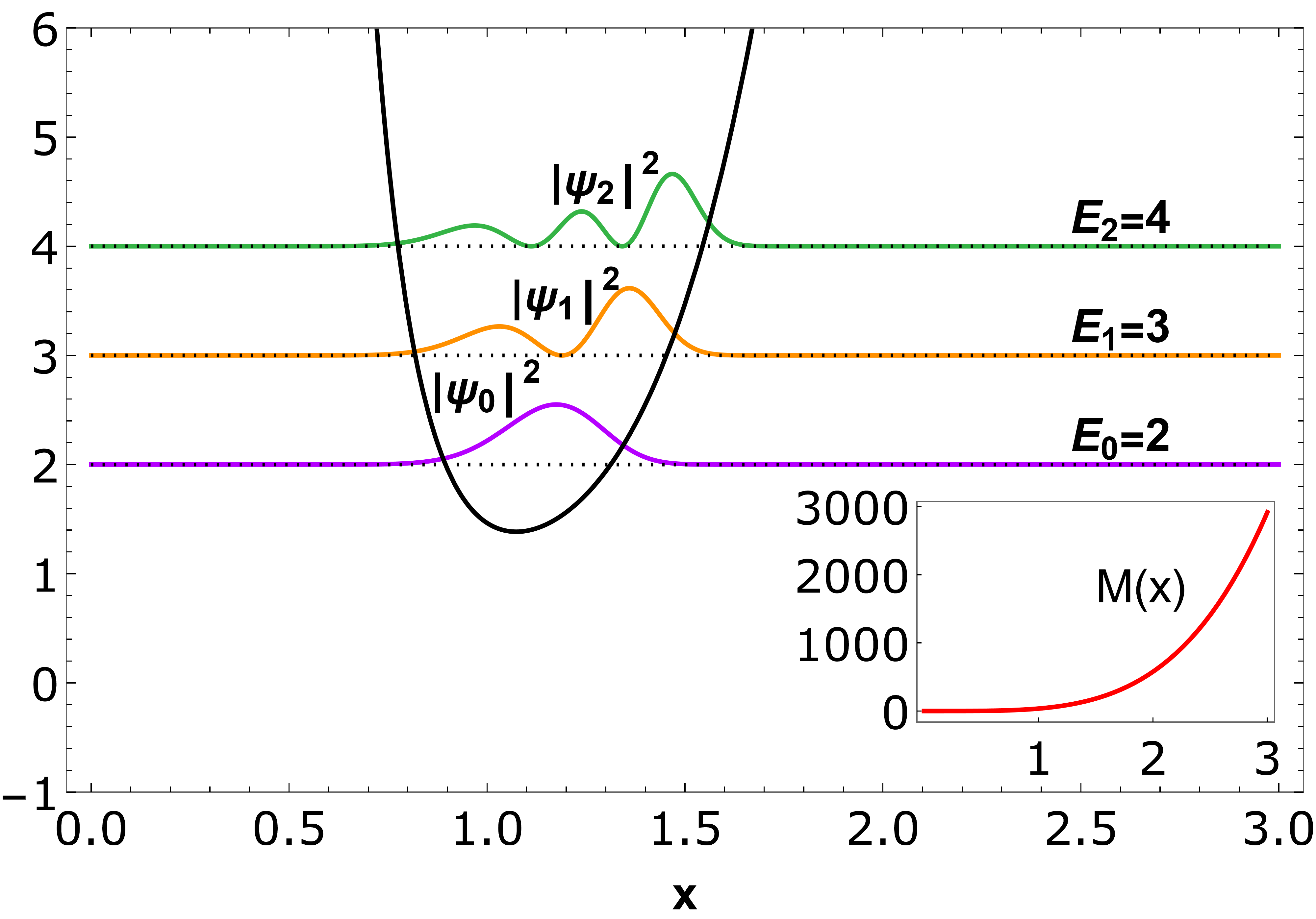
(c) $m=1,\nu=\frac{4}{5}$

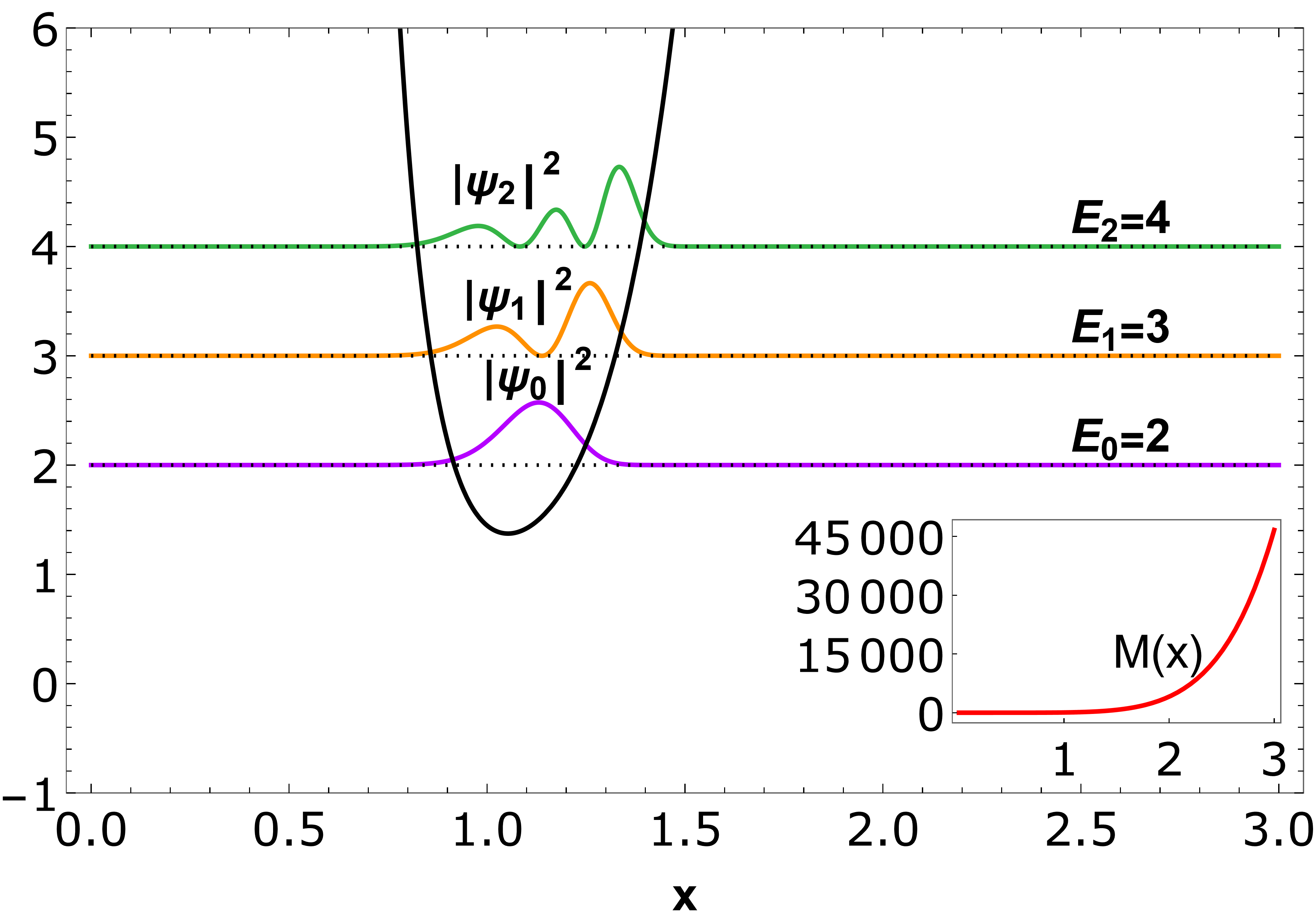
(d) $m=1,\nu=\frac{6}{7}$

Figure 2: Plot of the potential $V_{eff}$ given in Eq. (3.2) for $m=1$ and different $\nu$ values, square of first three bound state wavefunctions ${|\psi_{0}|}^{2}$ (purple line), ${|\psi_{1}|}^{2}$ (orange line), ${|\psi_{2}|}^{2}$ (green line) corresponding to different $\nu$ values, for mass function $M(x)$ (red line). We have consider here $\alpha=2$.

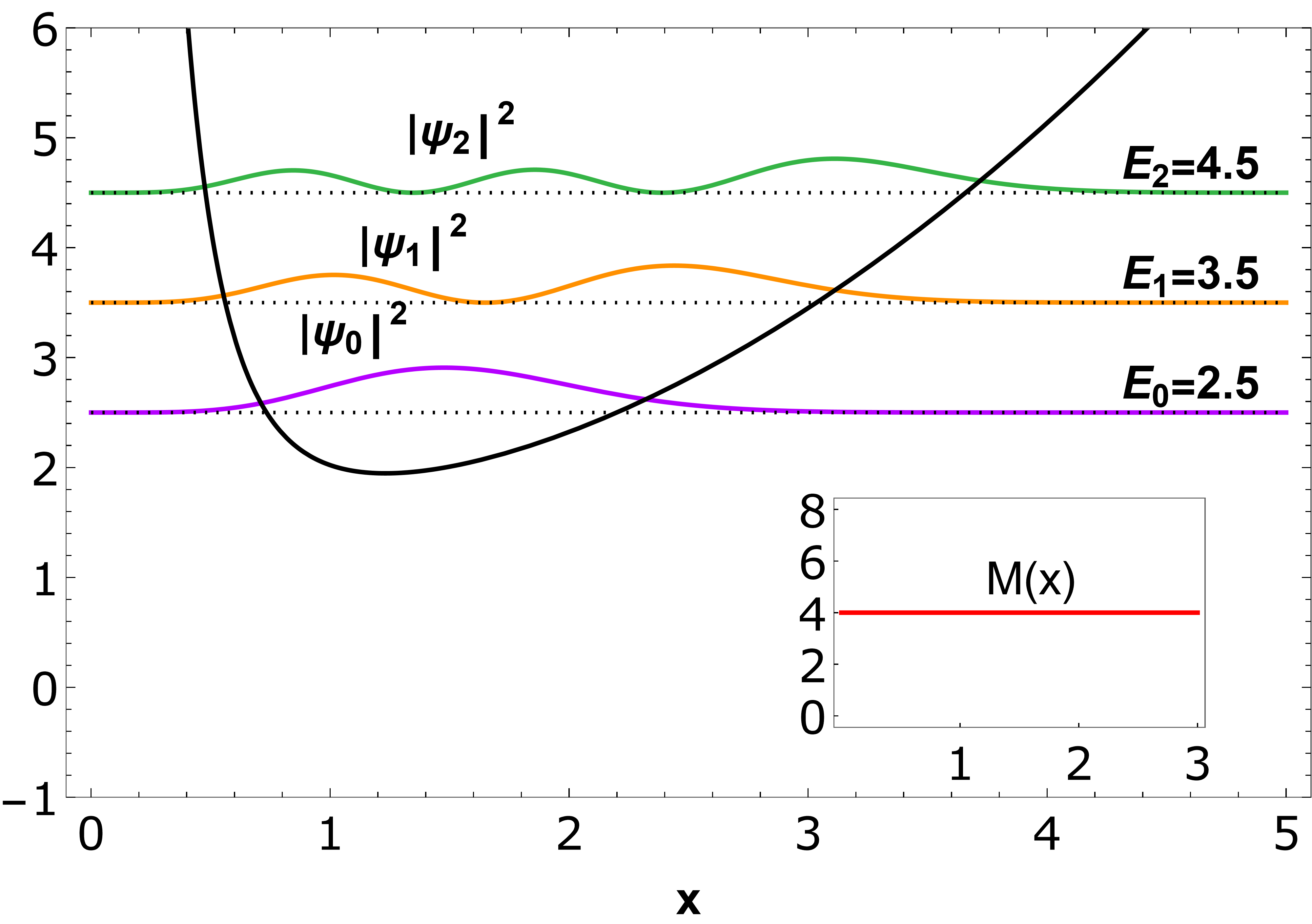
(a) $m=2,\nu=0$

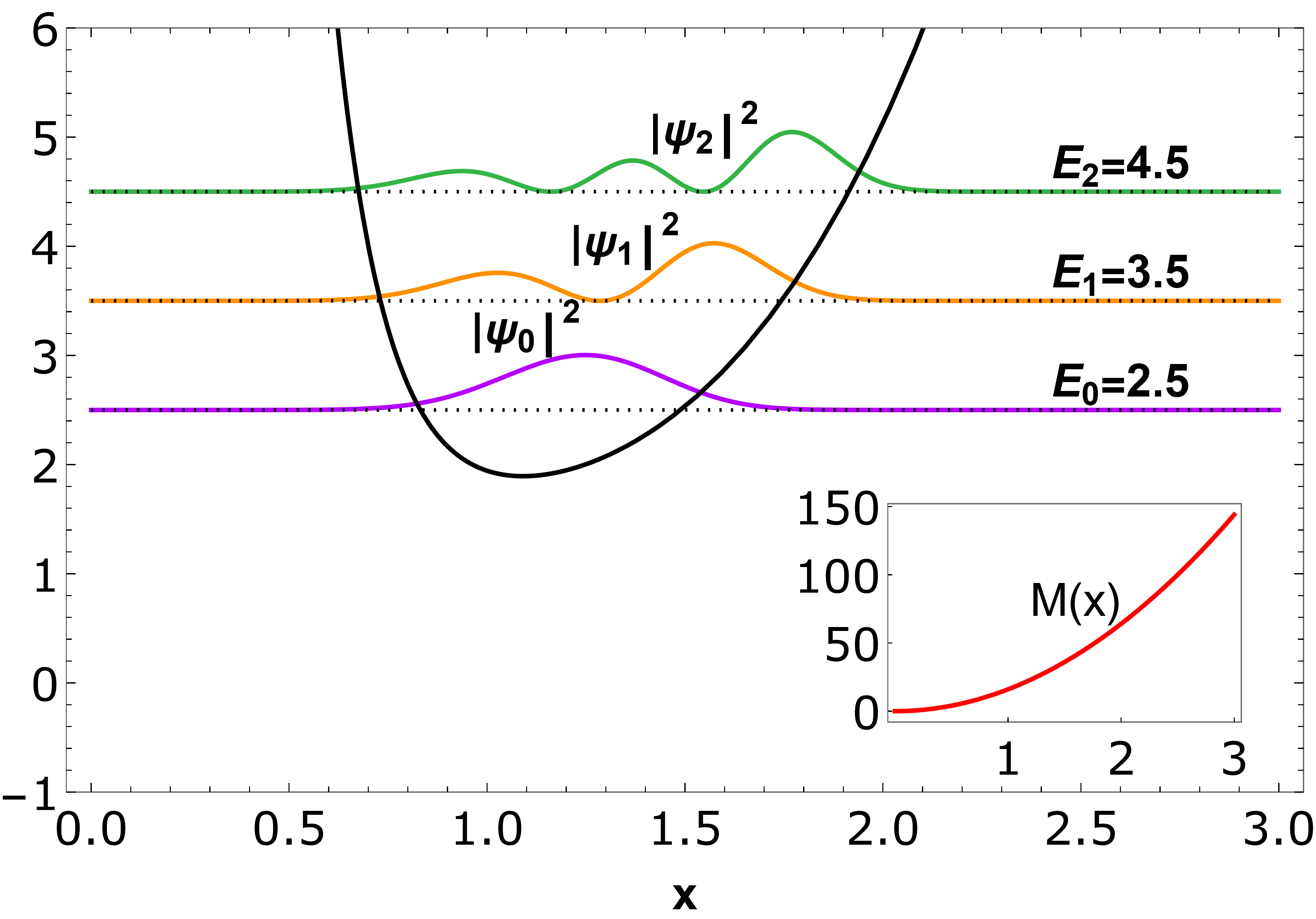
(b) $m=2,\nu=\frac{2}{3}$

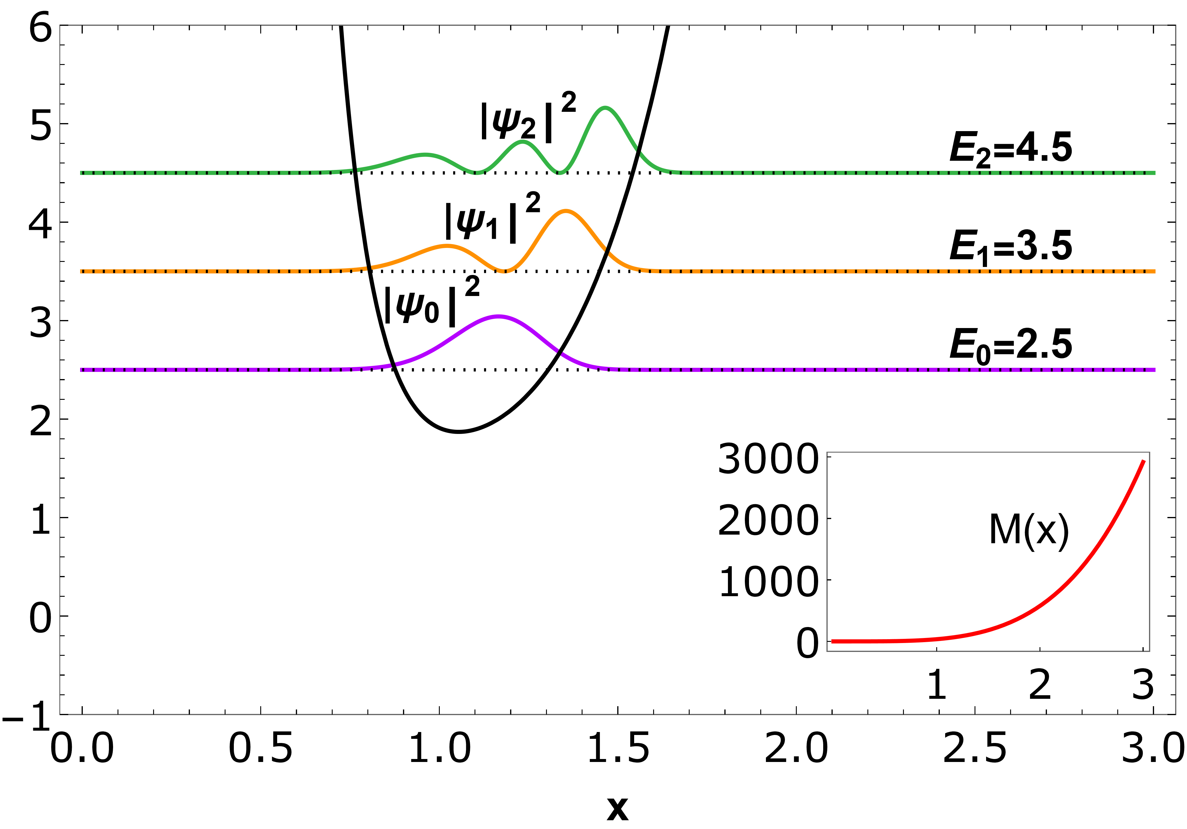
(c) $m=2,\nu=\frac{4}{5}$

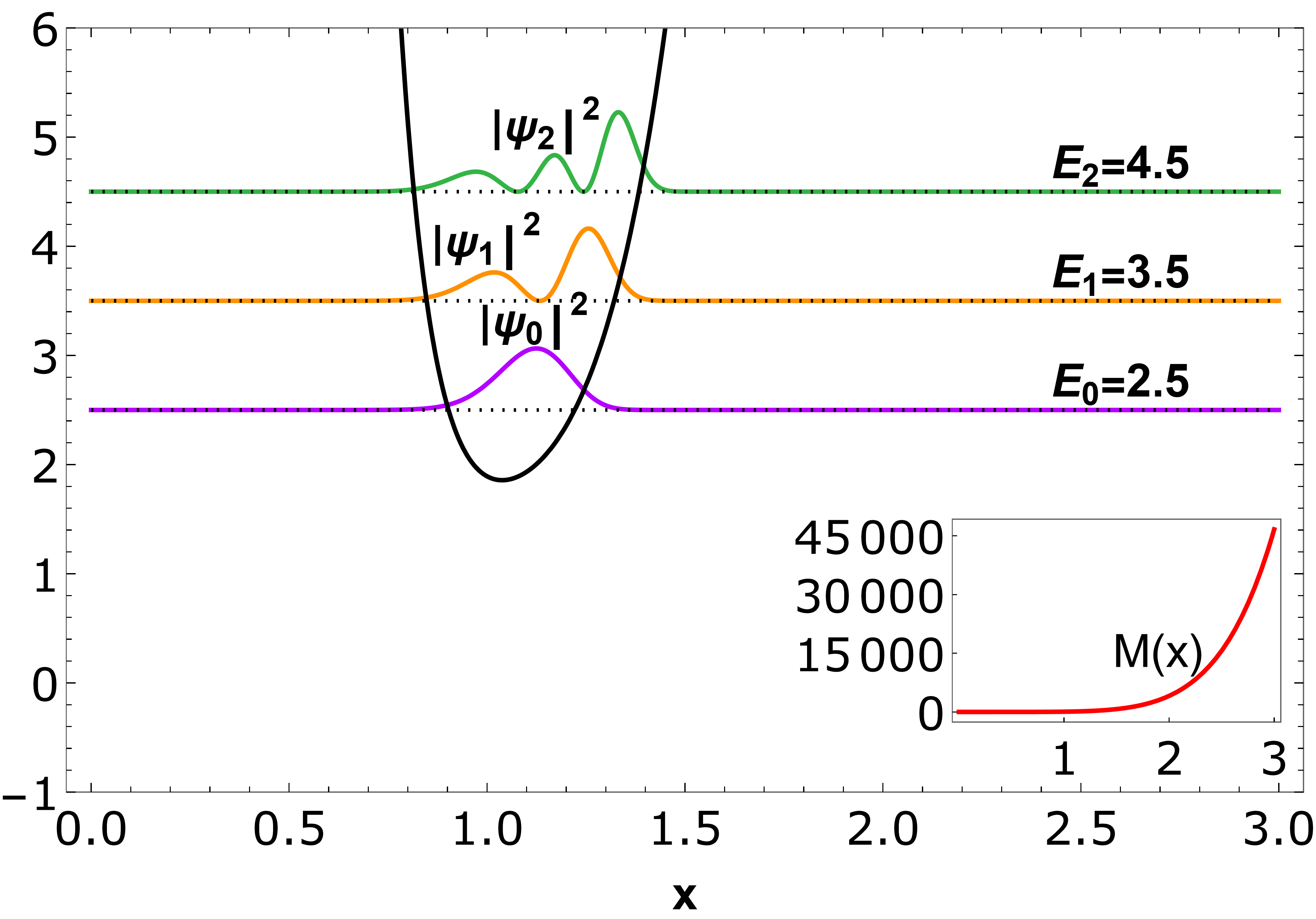
(d) $m=2,\nu=\frac{6}{7}$

Figure 3: Plot of the potential $V_{eff}$ given in Eq. (3.2) for $m=2$ and different $\nu$ values, square of first three bound state wavefunctions ${|\psi_{0}|}^{2}$ (purple line), ${|\psi_{1}|}^{2}$ (orange line), ${|\psi_{2}|}^{2}$ (green line) corresponding to different $\nu$ values, for mass function $M(x)$ (red line). We have consider here $\alpha=2$

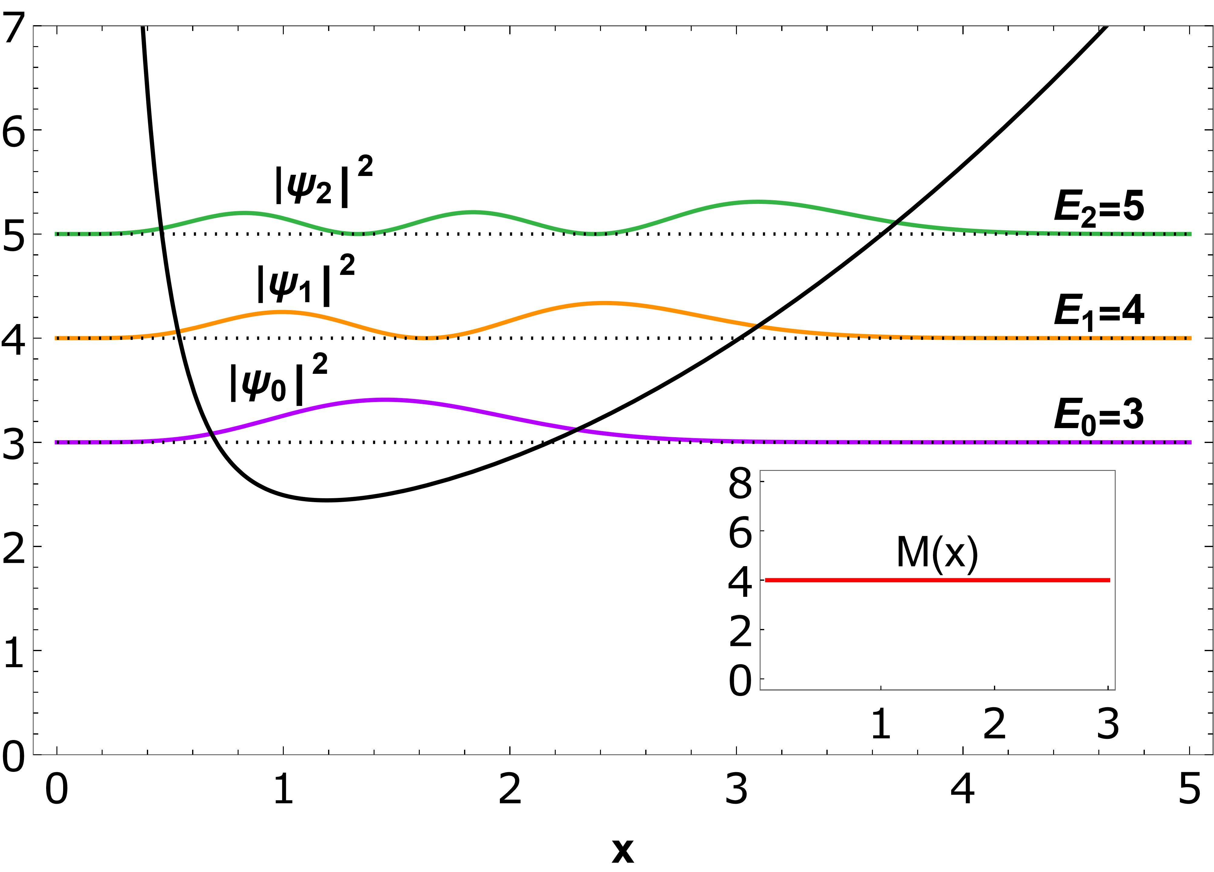
(a) $m=3,\nu=0$

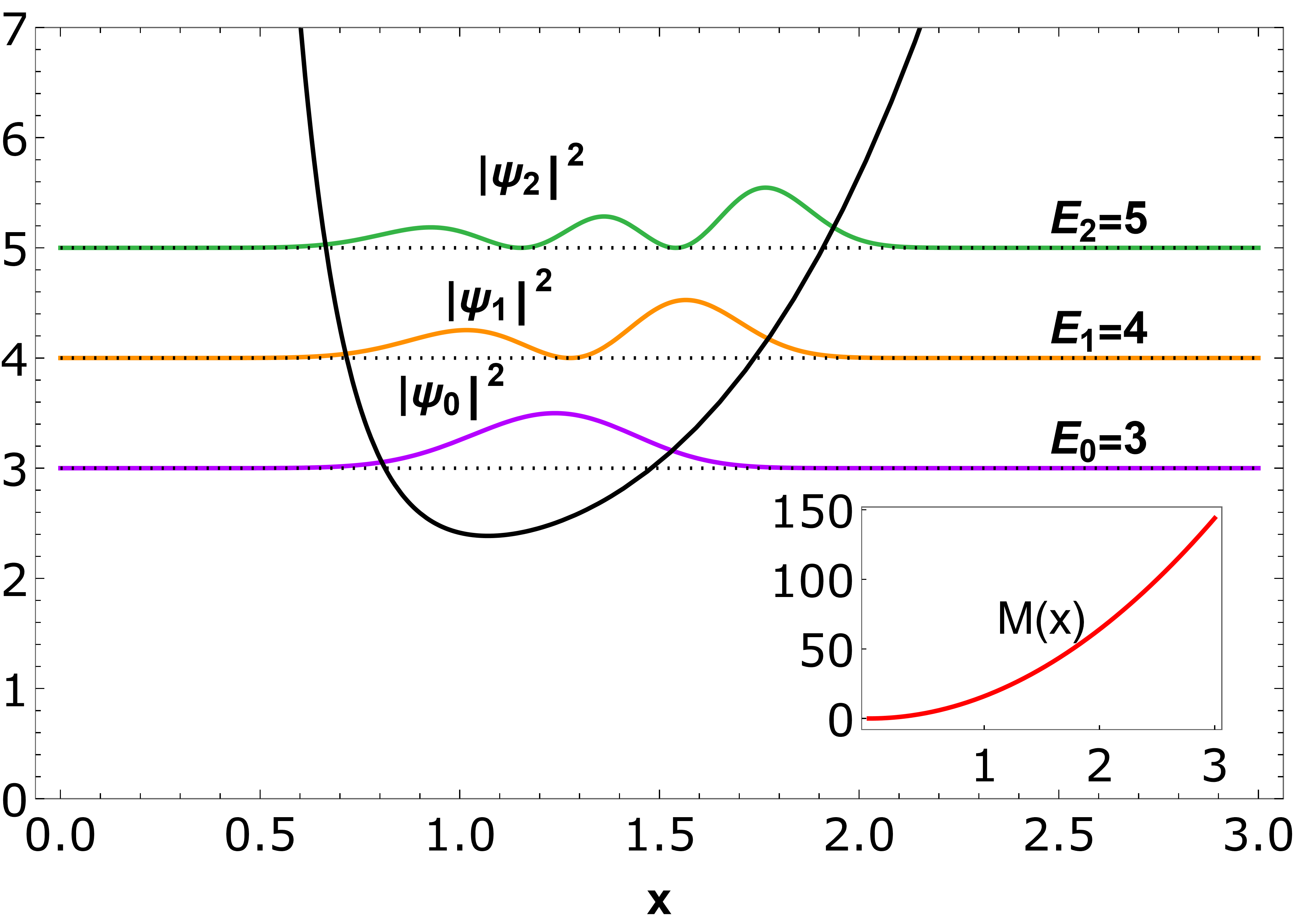
(b) $m=3,\nu=\frac{2}{3}$

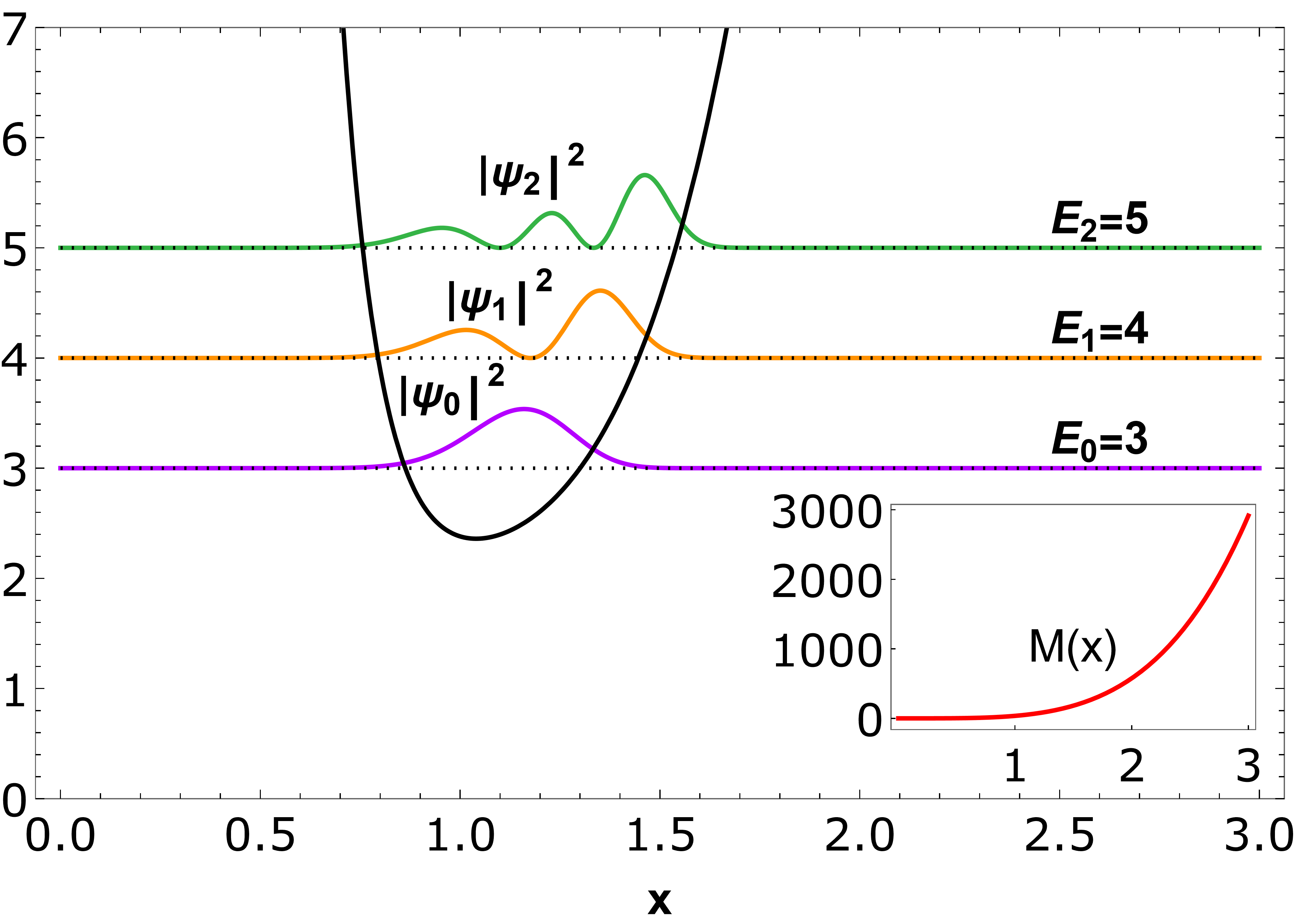
(c) $m=3,\nu=\frac{4}{5}$

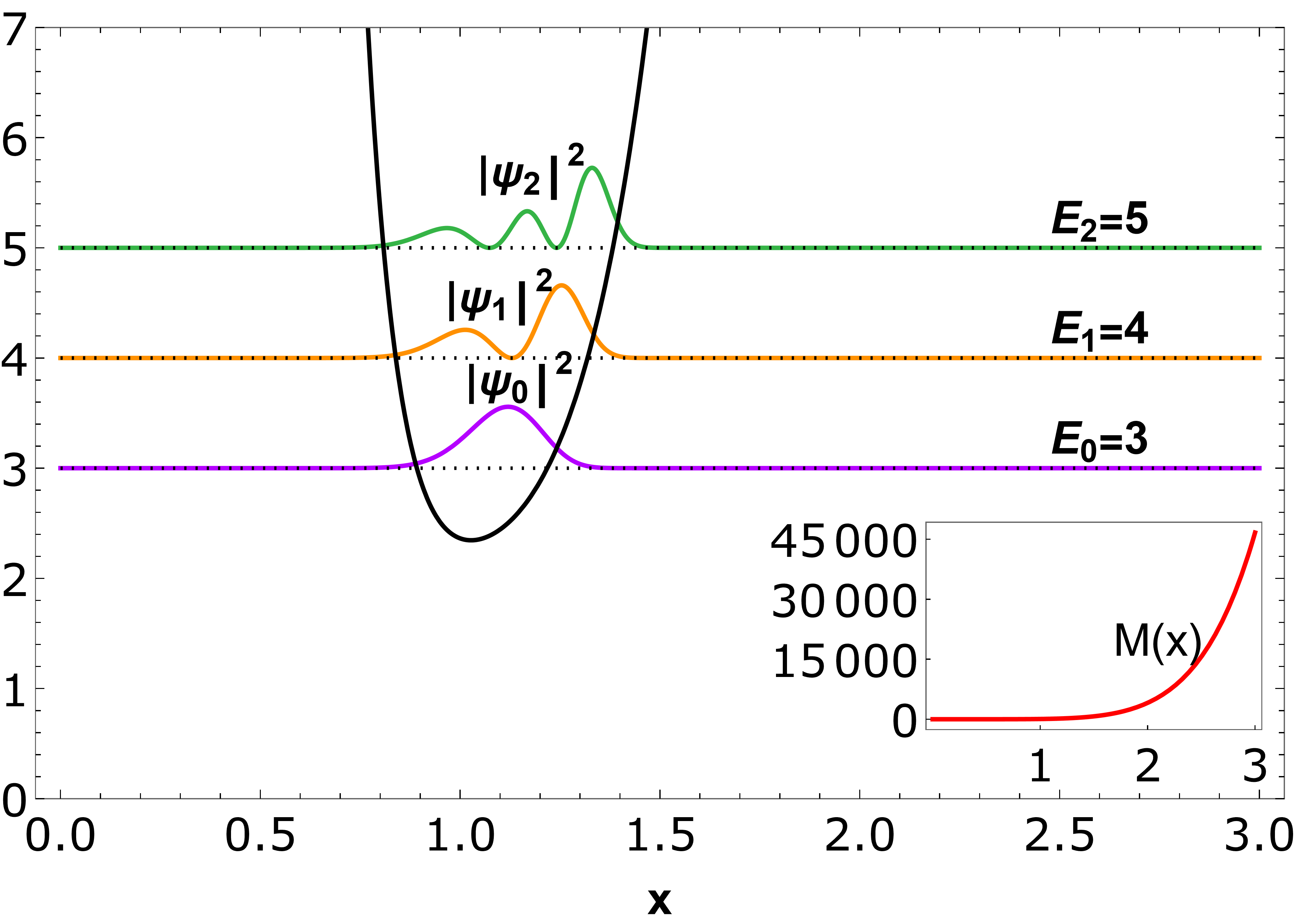
(d) $m=3,\nu=\frac{6}{7}$

Figure 4: Plot of the potential $V_{eff}$ given in Eq. (3.2) for $m=3$ and different $\nu$ values, square of first three bound state wavefunctions ${|\psi_{0}|}^{2}$ (purple line), ${|\psi_{1}|}^{2}$ (orange line), ${|\psi_{2}|}^{2}$ (green line) corresponding to different $\nu$ values, for mass function $M(x)$ (red line). We have considered here $\alpha=2$

We further generalise this analysis for the two dimensional case. The probability density of a two-dimensional potential is shown in the Fig. 5.

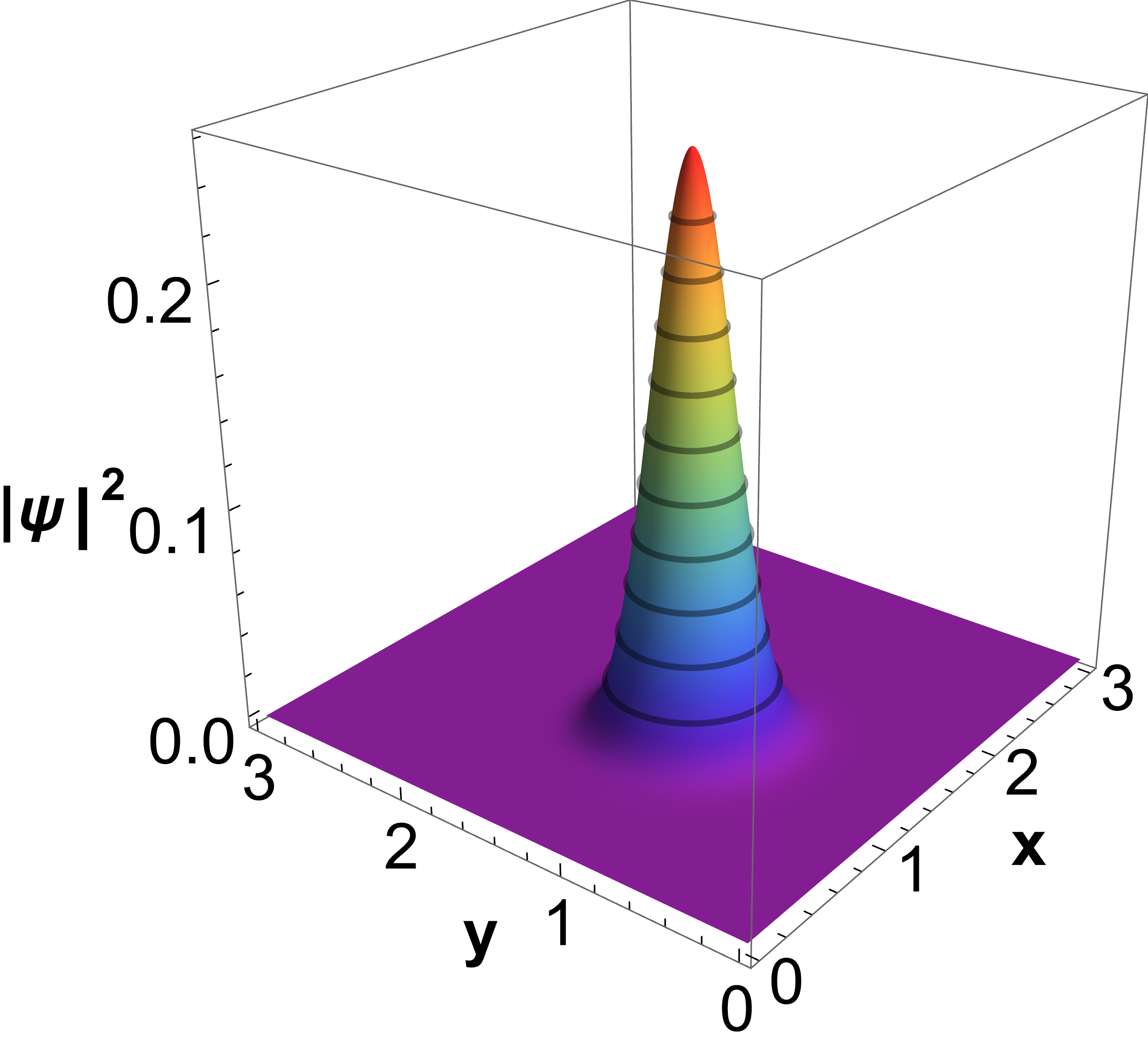
(a) $n_{1}=0,n_{2}=0$

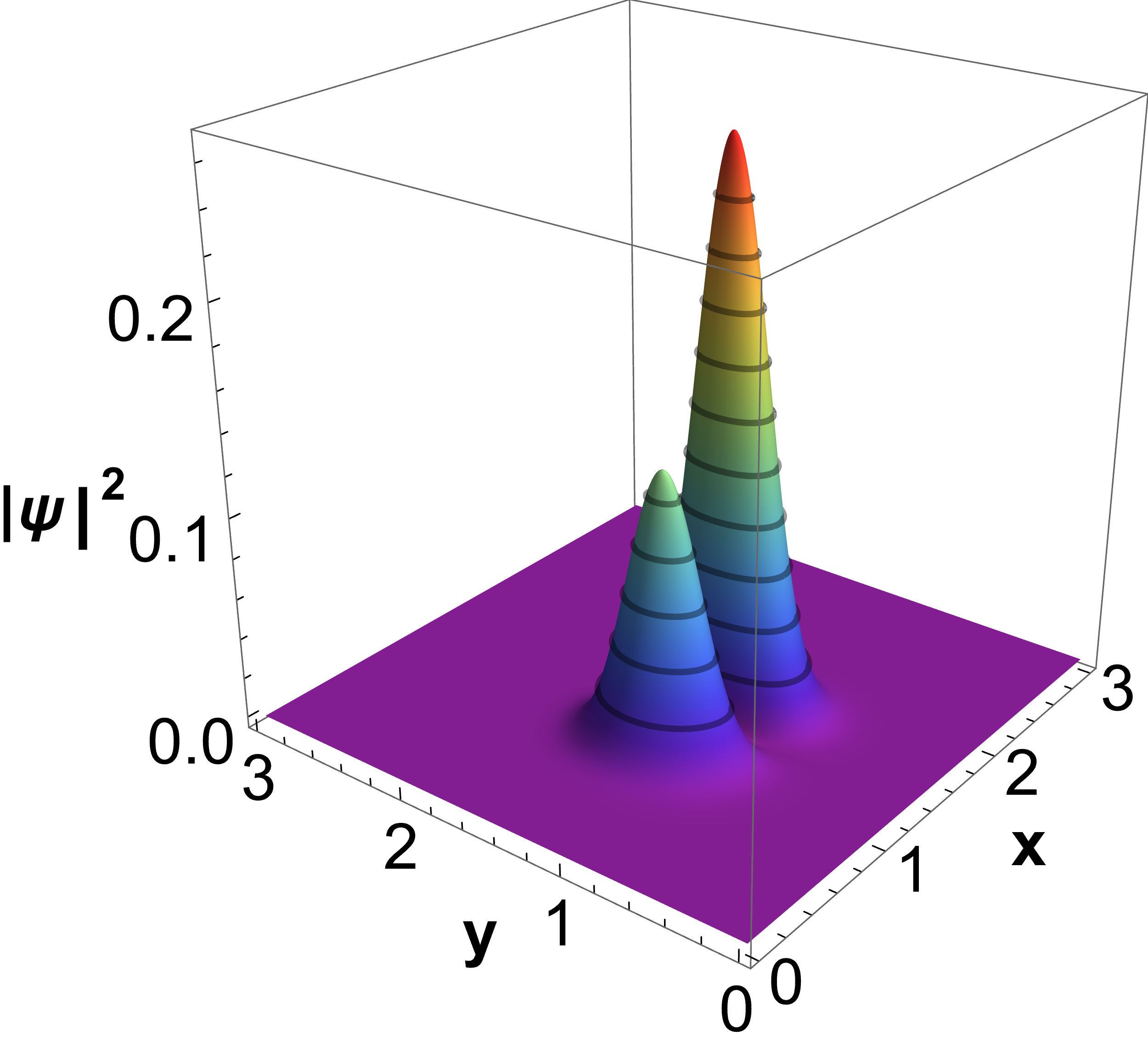
(b) $n_{1}=1,n_{2}=0$

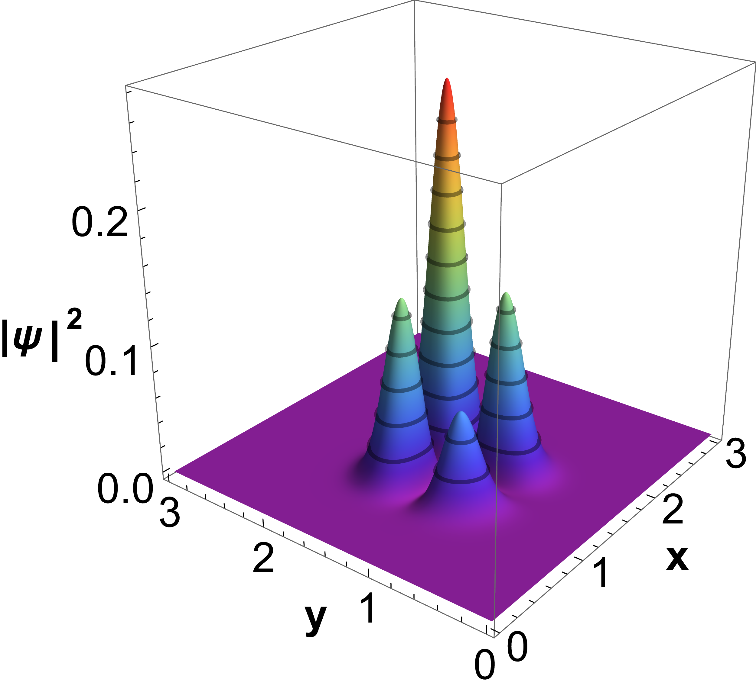
(c) $n_{1}=1,n_{2}=1$

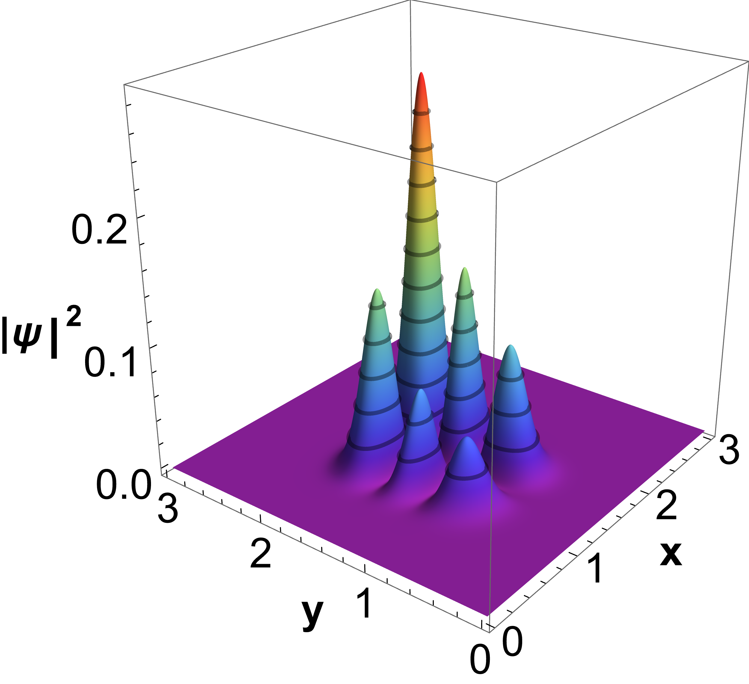
(d) $n_{1}=1,n_{2}=2$

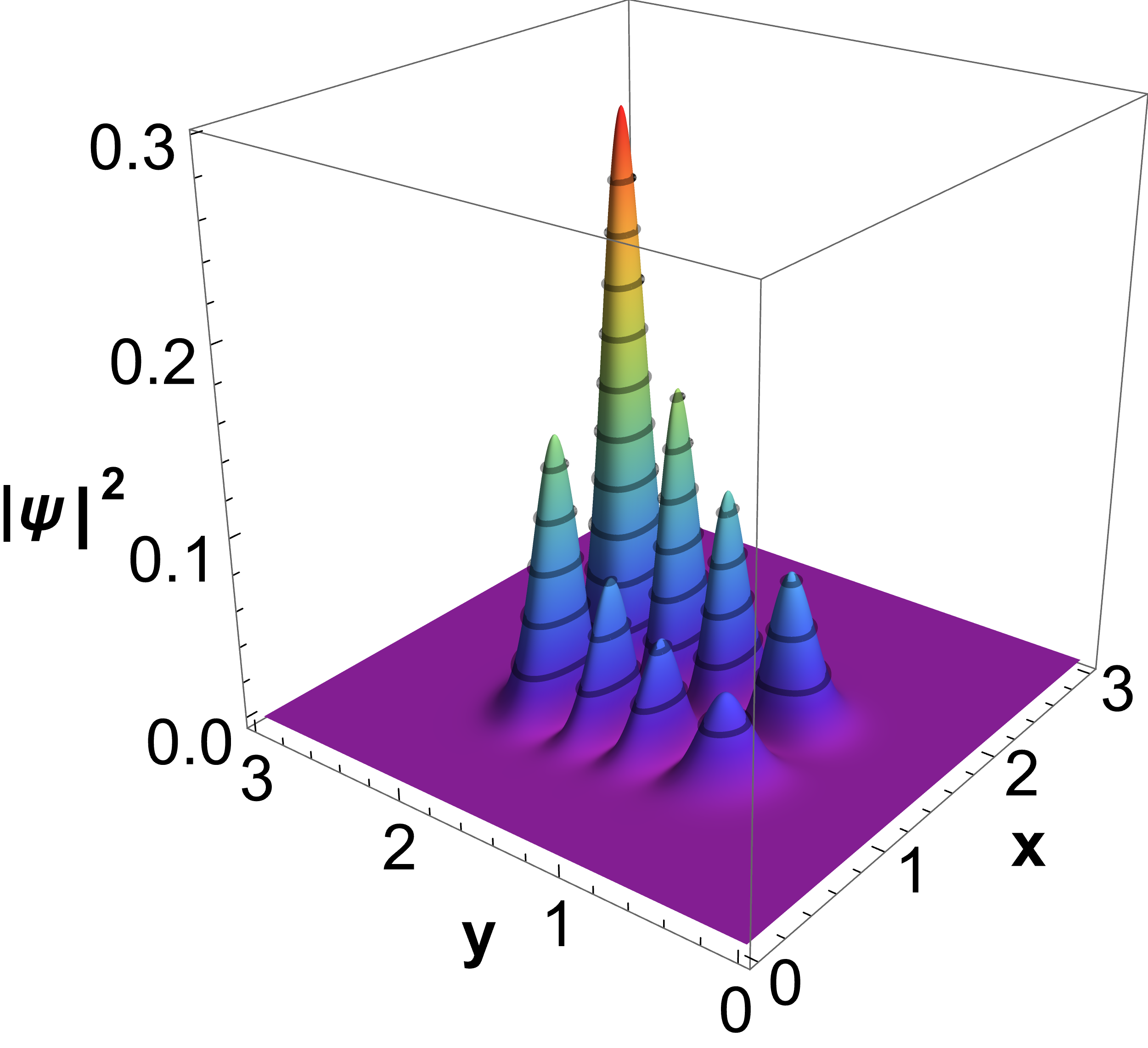
(e) $n_{1}=1,n_{2}=3$

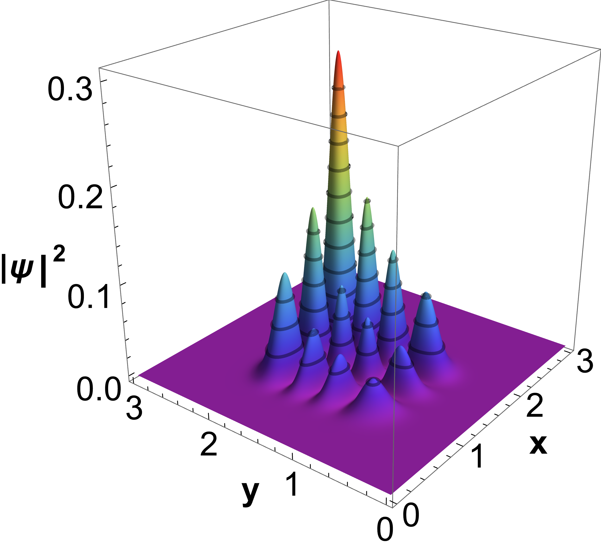
(f) $n_{1}=2,n_{2}=3$

Figure 5: Plot for the probability density of a two-dimensional potential for $m=1,\nu=\frac{2}{3}$ and different combinations of $n_{1}$ and $n_{2}$ values. The wavefunctions are normalized.

4 Supersymmetric approach

Within the context of supersymmetric quantum mechanics applied to systems with an effective mass, one can define the lowering and raising operator [61]

$$\mathcal{A}\psi=\frac{1}{\sqrt{M}}\frac{d\psi}{dx}+\mathcal{W}\psi,\quad\text{and }\quad\mathcal{A}^{\dagger}\psi=-\frac{d}{dx}\left(\frac{\psi}{\sqrt{M}}\right)+\mathcal{W}\psi$$ (35)

where $\mathcal{W}=-\frac{1}{\sqrt{M}}\frac{\psi_{0}^{{}^{\prime}}}{\psi_{0}}$ is the superpotential, and $\psi_{0}$ represents the ground state. The Hamiltonian for a system with an effective mass of (9) can be factorized as follows.

$$H_{eff}=\mathcal{A}^{\dagger}\mathcal{A}=-\frac{d}{dx}\left(\frac{1}{M(x)}\right)+V_{eff}$$ (36)

The associated supersymmetric partner Hamiltonian is given by

$$H_{eff}^{p}=\mathcal{A}\mathcal{A}^{\dagger}=-\frac{d}{dx}\left(\frac{1}{M(x)}\right)+V_{eff}^{p}$$ (37)

We see that both partner Hamiltonians $H_{eff}$ and $H_{eff}^{p}$ describe particles with identical spatial dependence on effective mass but in different potentials $V_{eff}$ and $V_{eff}^{p}$ respectively. These supersymmetric partner potentials are given by

$$V_{eff}=-\left(\frac{\mathcal{W}}{\sqrt{M}}\right)^{{}^{\prime}}+\mathcal{W}^{2}$$ (38)

$$V_{eff}^{p}=V_{eff}+\frac{2\mathcal{W}^{{}^{\prime}}}{\sqrt{M}}-\left(\frac{1}{\sqrt{M}}\right)\left(\frac{1}{\sqrt{M}}\right)^{{}^{\prime\prime}}$$ (39)

If these potentials are shape invariant, they must satisfy the condition

$$V_{eff}^{p}(x,a_{1})=V_{eff}(x,a_{2})+R(a_{1})$$ (40)

where $a_{1}$ is a set of parameters, $a_{2}$ is some function of $a_{1}$ and $R(a_{1})$ is independent of x. For unbroken supersymmetry, the eigenvalues and the eigenfunctions of the two such Hamiltonians with position-dependent effective mass are related by $(n=0,1,2,...)$

$$E_{n}^{eff,p}=E_{n+1}^{eff},~{}~{}~{}~{}~{}~{}E_{0}^{eff}=0$$ (41)

$$\psi_{n}^{eff,p}=[E_{n+1}^{eff}]^{-\frac{1}{2}}\mathcal{A}\psi_{n+1}^{eff}$$ (42)

$$\psi_{n+1}^{eff}=[E_{n}^{eff,1}]^{-\frac{1}{2}}\mathcal{A}^{\dagger}\psi_{n}^{eff,1}$$ (43)

The superpotential, corresponding to the potentials derived in case $1$ and case $2$ in the previous section, can be expressed as

$$\mathcal{W}^{I}=\frac{b}{2}\left((1+\alpha)e^{\frac{bx}{2}}-e^{\frac{-bx}{2}}\left(1+2\left(\frac{L_{m-1}^{\alpha}(-e^{-bx})}{{L_{m}^{\alpha-1}(-e^{-bx})}}-\frac{L_{m-1}^{\alpha+1}(-e^{-bx})}{{L_{m}^{\alpha}(-e^{-bx})}}\right)\right)\right)$$ (44)

and

$$\mathcal{W}^{II}=\left(\frac{1}{2}-\left(\frac{L_{m-1}^{\alpha+1}\left(-x^{l}\right)}{L_{m}^{\alpha}\left(-x^{l}\right)}-\frac{L_{m-1}^{\alpha}\left(-x^{l}\right)}{L_{m}^{\alpha-1}\left(-x^{l}\right)}\right)\right)x^{\frac{l}{2}}+\frac{1-l(\alpha+1)}{2l}x^{-\frac{l}{2}}$$ (45)

respectively, where $l=\frac{2-\nu}{1-\nu}$.
From the superpotential $\mathcal{W}^{I}$ (for case $1$), the partner potentials can be derived using equations (38) and (39)

$$V_{eff}^{I} =\frac{b^{2}}{4}\left(e^{bx}\left(\alpha^{2}-1\right)+e^{-bx}\right)+b^{2}\Bigg{(}\frac{2{L_{m-1}^{\alpha}(-e^{-bx})}^{2}}{({L_{m}^{\alpha-1}(-e^{-bx})})^{2}}-\frac{{L_{m-2}^{\alpha+1}(-e^{-bx})}}{{L_{m}^{\alpha-1}(-e^{-bx})}}+\frac{{L_{m-1}^{\alpha+1}(-e^{-bx})}}{\alpha{L_{m}^{\alpha-1}(-e^{-bx})}}$$

$$\quad+\frac{{L_{m-1}^{\alpha}(-e^{-bx})}}{{L_{m}^{\alpha-1}(-e^{-bx})}}-\frac{{L_{m-1}^{\alpha+1}(-e^{-bx})}}{{L_{m}^{\alpha-1}(-e^{-bx})}}\Bigg{)}e^{-bx}-b^{2}\left(\frac{2m+\alpha+\alpha^{2}}{2\alpha}\right)$$ (46)

$$V_{eff}^{I,p} =\frac{b^{2}}{4}\left(e^{bx}\alpha\left(\alpha+2\right)+e^{-bx}\right)+b^{2}\Bigg{(}\frac{2{L_{m-1}^{\alpha+1}(-e^{-bx})}^{2}}{({L_{m}^{\alpha}(-e^{-bx})})^{2}}-\frac{{L_{m-2}^{\alpha+2}(-e^{-bx})}}{{L_{m}^{\alpha}(-e^{-bx})}}+\frac{{L_{m-1}^{\alpha+2}(-e^{-bx})}}{\alpha{L_{m}^{\alpha}(-e^{-bx})}}$$

$$\quad+\frac{{L_{m-1}^{\alpha+1}(-e^{-bx})}}{{L_{m}^{\alpha}(-e^{-bx})}}-\frac{{L_{m-1}^{\alpha+2}(-e^{-bx})}}{{L_{m}^{\alpha}(-e^{-bx})}}\Bigg{)}e^{-bx}-b^{2}\left(\frac{\alpha+1}{2}+\frac{m}{\alpha+2}\right)$$ (47)

Also from superpotential $\mathcal{W}^{II}$ (for case $2$) and equations (38) and (39) we can write the partner potentials

$$V^{II}_{eff} =\frac{1}{4}\left(x^{\frac{\nu-2}{1-\nu}}\left(\alpha^{2}-1\right)+x^{\frac{2-\nu}{1-\nu}}\right)+\Bigg{(}\frac{2{L_{m-1}^{\alpha}(-x^{\frac{2-\nu}{1-\nu}})}^{2}}{({L_{m}^{\alpha-1}(-x^{\frac{2-\nu}{1-\nu}})})^{2}}-\frac{{L_{m-2}^{\alpha+1}(-x^{\frac{2-\nu}{1-\nu}})}}{{L_{m}^{\alpha-1}(-x^{\frac{2-\nu}{1-\nu}})}}+\frac{{L_{m-1}^{\alpha+1}(-x^{\frac{2-\nu}{1-\nu}})}}{\alpha{L_{m}^{\alpha-1}(-x^{\frac{2-\nu}{1-\nu}})}}$$

$$\quad+\frac{{L_{m-1}^{\alpha}(-x^{\frac{2-\nu}{1-\nu}})}}{{L_{m}^{\alpha-1}(-x^{\frac{2-\nu}{1-\nu}})}}-\frac{{L_{m-1}^{\alpha+1}(-x^{\frac{2-\nu}{1-\nu}})}}{{L_{m}^{\alpha-1}(-x^{\frac{2-\nu}{1-\nu}})}}\Bigg{)}x^{\frac{2-\nu}{1-\nu}}+\frac{(1-\nu)(3-\nu)}{4{(2-\nu)}^{2}}x^{\frac{\nu-2}{1-\nu}}-\frac{2m+\alpha+\alpha^{2}}{2\alpha}$$ (48)

and

$$V^{II,p}_{eff} =\frac{1}{4}\left(x^{\frac{\nu-2}{1-\nu}}\alpha(\alpha+2)+x^{\frac{2-\nu}{1-\nu}}\right)+\Bigg{(}\frac{2{L_{m-1}^{(\alpha+1)}(-x^{\frac{2-\nu}{1-\nu}})}^{2}}{({L_{m}^{\alpha}(-x^{\frac{2-\nu}{1-\nu}})})^{2}}-\frac{{L_{m-2}^{(\alpha+2)}(-x^{\frac{2-\nu}{1-\nu}})}}{{L_{m}^{\alpha}(-x^{\frac{2-\nu}{1-\nu}})}}+\frac{{L_{m-1}^{(\alpha+2)}(-x^{\frac{2-\nu}{1-\nu}})}}{(\alpha+1){L_{m}^{\alpha}(-x^{\frac{2-\nu}{1-\nu}})}}$$

$$\quad+\frac{{L_{m-1}^{(\alpha+1)}(-x^{\frac{2-\nu}{1-\nu}})}}{{L_{m}^{\alpha}(-x^{\frac{2-\nu}{1-\nu}})}}-\frac{{L_{m-1}^{(\alpha+2)}(-x^{\frac{2-\nu}{1-\nu}})}}{{L_{m}^{\alpha}(-x^{\frac{2-\nu}{1-\nu}})}}\Bigg{)}x^{\frac{2-\nu}{1-\nu}}+\frac{(1-\nu)(3-\nu)}{4{(2-\nu)}^{2}}x^{\frac{\nu-2}{1-\nu}}-\left(\frac{\alpha}{2}+\frac{m}{\alpha+1}\right)$$ (49)

The potentials $V^{I}_{eff}$ and $V^{II}_{eff}$ obtained in Eq.(4) and (4)are same with potentials in Eq. (3.1) and (3.2) for $V^{I}_{c}=-b^{2}\left(\frac{2m+\alpha+\alpha^{2}}{2\alpha}\right)$ and $V^{II}_{c}=-\frac{2m+\alpha+\alpha^{2}}{2\alpha}$ respectively.
From Eqs. (4) and (4), we note that the potential and its supersymmetric counterpart satisfy the condition

$$V^{I,p}_{eff}(x,\alpha)=V^{I}_{eff}(x,\alpha+1)+b^{2}$$ (50)

Also from Eqs. (4) and (4) we see that the partner potentials satisfy the similar relation

$$V^{II,p}_{eff}(x,\alpha)=V^{II}_{eff}(x,\alpha+1)+1$$ (51)

It’s evident that the potentials obtained for case $1$ and case $2$ satisfy the condition of shape invariant potentials given in Eq. (40). Thus, we deduce that the newly introduced potentials exhibit shape invariance.
We’ve deduced the eigenstates for the partner potential associated with potential (3.1) as

$$\psi^{p}_{n,m}(x)=\propto\frac{\exp{[-\frac{1}{2}((\alpha+2)bx+e^{-bx})]}}{L_{m}^{\alpha}(-e^{-bx})}\hat{L}_{n+m,m}^{\alpha+1}(e^{-bx})~{}~{}~{}n=0,1,2,...$$ (52)

and the eigenstate of the partner potential of Eq. (3.2) is given by

$$\psi^{p}_{n,m}(x)\propto\frac{\exp\left(\frac{-x^{\frac{2-\nu}{1-\nu}}}{2}\right)}{\left(L_{m}^{\alpha}(-x^{\frac{2-\nu}{1-\nu}})\right)}x^{\frac{(2+\alpha)+(\alpha+1)(1-\nu)}{2(1-\nu)}}\hat{L}_{n+m,m}^{\alpha+1}(x^{\frac{2-\nu}{1-\nu}}),~{}~{}~{}~{}n=0,1,2,...$$ (53)

5 Results and Discussions

The study of systems endowed with position-dependent mass (PDM) is a subject of great interest in many branches of physics due to its utmost relevance in a wide variety of physical situations. However only a few PDM systems are solved exactly for some specific position dependent of Mass terms, i.e. $M(x)\propto[g^{\prime}(x)]^{\mu}$ for $\mu=1,2$ and $-1$. In this article we have considered a new type of position dependent mass term, which is proportional to $\left({g^{\prime}(x)}\right)^{\nu}$,  $\nu=\frac{2\eta}{2\eta+1},$ with $\eta=0,1,2\cdots$ and have obtained the solutions of position-dependent mass Schrödinger equation in terms of $X_{m}$ Laguerre polynomials. Furthermore, we have obtained one parameter family of isochronous potentials, which are exactly solvable. The solution corresponding to these potentials are shown to be in terms of $X_{m}$ Laguerre polynomials. We have shown the SUSY for PDM systems and for this system, we find the one-parameter family of isochronous potentials and its partner potentials. We show the exact solvability of the system is due to the underlying shape invariance of these SUSY potentials.

Acknowledgments: BPM acknowledges the support from the research grant under IoE scheme (Number - 6031), BHU, UGC Government of India. SY acknowledges the fruitful discussion with Sudhanshu Shekhar, BHU. RG acknowledges the financial support from IOE, BHU for a short visit to BHU during which some part of the work has been carried out.

References

• [1] D. G. W. Parfitt, M. E. Portnoi, The two-dimensional hydrogen atom revisited, J. Math. Phys. 43 (10) (2002) 4681–4691. doi:10.1063/1.1503868.
• [2] F. Cooper, A. Khare, U. Sukhatme, Supersymmetry and quantum mechanics, Phys. Rep. 251 (1995) 267. doi:10.1016/0370-1573(94)00080-M.
• [3] B. Bagchi, Supersymmetry in Quantum and Classical Mechanics, Chapman and Hall; CRC, 2000.
• [4] D. J. F. C, Supersymmetric quantum mechanics, AIP Conf. Proc. 1287 (2010) 3. doi:10.1063/1.3507423.
• [5] G. Junker, Supersymmetric methods in quantum and statistical physics, Springer Science & Business Media, 2012.
• [6] A. Gangopadhyaya, J. Mallow, C. Rasinariu, Supersymmetric Quantum Mechanics: An Introduction, World Scientific, 2017.
• [7] S. Yadav, A. Khare, B. P. Mandal, Supersymmetry and shape invariance of exceptional orthogonal polynomials, Ann. Phys. 444 (2022) 169064. doi:10.1016/j.aop.2022.169064.
• [8] J. Wu, Y. Alhassid, The potential group approach and hypergeometric differential equations, J. Math. Phys. 31 (1990) 557. doi:10.1063/1.528889.
• [9] M. J. Englefield, C. Quesne, Potentials generated by su (1, 1), J. Phys. A: Math. Gen. 24 (1991) 827. doi:10.1088/0305-4470/24/15/023.
• [10] B. Bagchi, R. Ghosh, C. Quesne, so(2, 1) algebra, local Fermi velocity, and position-dependent mass Dirac equation, J. Phys. A 55 (37) (2022) 375204. doi:10.1088/1751-8121/ac8588.
• [11] M. F. Manning, Exact solutions of the schrödinger equation, Phys. Rev. 48 (2) (1935) 161–164. doi:10.1103/PhysRev.48.161.
• [12] C. A. Downing, On a solution of the schrödinger equation with a hyperbolic double-well potential, J. Math. Phys. 54 (7). doi:10.1063/1.4811855.
• [13] H. Hassanabadi, S. Zarrinkamar, A. A. Rajabi, A simple efficient methodology for dirac equation in minimal length quantum mechanics, Phys. Lett. B 718 (2013) 1111. doi:10.1016/j.physletb.2012.11.044.
• [14] R. Ghosh, Solving non-hermitian dirac equation in the presence of pdm and local fermi velocity, Int. J. Mod. Phys. A 37 (36) (2022) 2250222. doi:10.1142/S0217751X22502220.
• [15] P. Harrison, A. Valavanis, Quantum wells, wires and dots: theoretical and computational physics of semiconductor nanostructures, John Wiley & Sons, 2016.
• [16] K. X. Guo, S. W. Gu, Nonlinear optical rectification in parabolic quantum wells with an applied electric field, Phys. Rev. B 47 (24) (1993) 16322–16325. doi:10.1103/PhysRevB.47.16322.
• [17] H. El Ghazi, A. Jorio, I. Zorkani, Linear and nonlinear intra-conduction band optical absorption in (in, ga) n/gan spherical qd under hydrostatic pressure, Optics Communications 331 (2014) 73–76. doi:10.1016/j.optcom.2014.05.055.
• [18] M. R. K. Vahdani, The effect of the electronic intersubband transitions of quantum dots on the linear and nonlinear optical properties of dot-matrix system, Superlattices and Microstructures 76 (2014) 326–338. doi:10.1016/j.spmi.2014.09.023.
• [19] G. Bastard, Wave mechanics applied to semiconductor heterostructures, New York, NY (USA); John Wiley and Sons Inc., 1990.
• [20] M. R. Geller, W. Kohn, Quantum mechanics of electrons in crystals with graded composition, Phys. Rev. Lett. 70 (1993) 3103. doi:10.1103/PhysRevLett.70.3103.
• [21] L. Serra, E. Lipparini, Spin response of unpolarized quantum dots, Europhys. Lett. 40 (1997) 667. doi:10.1209/epl/i1997-00520-y.
• [22] M. Barranco, M. Pi, S. M. Gatica, E. S. Hernández, J. Navarro, Structure and energetics of mixed helium-4 - helium-3 drops, Phys. Rev. B 56 (1997) 8997. doi:10.1103/physrevb.56.8997.
• [23] W. Miller, S. Post, P. Winternitz, Classical and quantum superintegrability with applications, J. Phys. A Math. Theor. 46 (42) (2013) 423001. doi:10.1088/1751-8113/46/42/423001.
• [24] I. Marquette, P. Winternitz, Superintegrable systems with third-order integrals of motion, J. Phys. A Math. Theor. 41 (30) (2008) 304031. doi:10.1088/1751-8113/41/30/304031.
• [25] W. M. C. Foulkes, L. Mitas, R. J. Needs, G. Rajagopal, Quantum monte carlo simulations of solids, Rev. Mod. Phys. 73 (1) (2001) 33–83. doi:10.1103/RevModPhys.73.33.
• [26] R. M. Martin, Electronic structure: basic theory and practical methods, Cambridge university press, 2020.
• [27] A. Kempf, G. Mangano, R. B. Mann, Hilbert space representation of the minimal length uncertainty relation, Phys. Rev. D 52 (2) (1995) 1108. doi:10.1103/PhysRevD.52.1108.
• [28] A. Kempf, Information-theoretic natural ultraviolet cutoff for spacetime, Phys. Rev. Lett. 103 (23) (2009) 231301. doi:10.1103/PhysRevLett.103.231301.
• [29] C. Quesne, V. Tkachuk, Deformed algebras, position-dependent effective masses and curved spaces: an exactly solvable coulomb problem, Journal of Physics A: Mathematical and General 37 (14) (2004) 4267. doi:10.1088/0305-4470/37/14/006.
• [30] R. N. Costa Filho, M. P. Almeida, G. A. Farias, J. S. Andrade, Displacement operator for quantum systems with position-dependent mass, Phys. Rev. A 84 (5) (2011) 050102. doi:10.1103/PhysRevA.84.050102.
• [31] O. Mustafa, S. H. Mazharimousavi, Quantum particles trapped in a position-dependent mass barrier; a d-dimensional recipe, Phys. Lett. A 358 (2006) 259. doi:10.1016/j.physleta.2006.05.037.
• [32] F. S. A. Cavalcante, R. N. Costa Filho, J. R. Filho, C. A. S. de Almeida, V. N. Freire, Form of the quantum kinetic-energy operator with spatially varying effective mass, Phys. Rev. B 55 (3) (1997) 1326–1328. doi:10.1103/PhysRevB.55.1326.
• [33] D. J. BenDaniel, C. B. Duke, Space-charge effects on electron tunneling, Phys. Rev. 152 (1966) 683. doi:10.1103/physrev.152.683.
• [34] D. Gómez-Ullate, N. Kamran, R. Milson, An extended class of orthogonal polynomials defined by a sturm–liouville problem, J. Math. Ana. App. 359 (1) (2009) 352. doi:10.1016/j.jmaa.2009.05.052.
• [35] D. Gómez-Ullate, N. Kamran, R. Milson, Exceptional orthogonal polynomials and the darboux transformation, J. Phys. A Math. Theor. 43 (43) (2010) 434016. doi:10.1088/1751-8113/43/43/434016.
• [36] D. Gómez-Ullate, N. Kamran, R. Milson, On orthogonal polynomials spanning a non-standard flag, Contemp. Math 563 (2012) 51. doi:10.1090/conm/563/11164.
• [37] R. K. Yadav, A. Khare, N. Kumari, B. P. Mandal, Rationally extended many-body truncated calogero–sutherland model, Annals of Physics 400 (2019) 189–197. doi:10.1016/j.aop.2018.11.009.
• [38] R. K. Yadav, S. Banerjee, N. Kumari, A. Khare, B. P. Mandal, One parameter family of rationally extended isospectral potentials, Annals of Physics 436 (2022) 168679. doi:10.1016/j.aop.2021.168679.
• [39] N. Kumari, R. K. Yadav, A. Khare, B. P. Mandal, A class of exactly solvable rationally extended calogero–wolfes type 3-body problems, Annals of Physics 385 (2017) 57–69. doi:10.1016/j.aop.2017.07.022.
• [40] N. Kumari, R. K. Yadav, A. Khare, B. P. Mandal, A class of exactly solvable rationally extended non-central potentials in two and three dimensions, Journal of Mathematical Physics 59 (6). doi:10.1063/1.4996282.
• [41] N. Kumari, R. K. Yadav, A. Khare, B. Bagchi, B. P. Mandal, Scattering amplitudes for the rationally extended pt symmetric complex potentials, Annals of Physics 373 (2016) 163–177. doi:10.1016/j.aop.2016.07.024.
• [42] R. K. Yadav, A. Khare, B. P. Mandal, The scattering amplitude for a newly found exactly solvable potential, Annals of Physics 331 (2013) 313–316. doi:10.1016/j.aop.2013.01.006.
• [43] R. K. Yadav, A. Khare, B. P. Mandal, The scattering amplitude for one parameter family of shape invariant potentials related to xm jacobi polynomials, Physics Letters B 723 (4-5) (2013) 433–435. doi:10.1016/j.physletb.2013.05.036.
• [44] D. Dutta, P. Roy, Conditionally exactly solvable potentials and exceptional orthogonal polynomials, Journal of Mathematical Physics 51 (4). doi:10.1063/1.3339676.
• [45] B. Midya, B. Roy, Exceptional orthogonal polynomials and exactly solvable potentials in position dependent mass schrödinger hamiltonians, Phys. Lett. A 373 (45) (2009) 4117. doi:10.1016/j.physleta.2009.09.030.
• [46] F. H. Stillinger, D. K. Stillinger, Pseudoharmonic oscillators and inadequacy of semiclassical quantization, The Journal of Physical Chemistry 93 (19) (1989) 6890–6892. doi:10.1021/j100356a004.
• [47] J. Dorignac, On the quantum spectrum of isochronous potentials, Journal of Physics A: Mathematical and General 38 (27) (2005) 6183. doi:10.1088/0305-4470/38/27/007.
• [48] B. Bagchi, P. Gorain, C. Quesne, R. Roychoudhury, New approach to (quasi-) exactly solvable schrödinger equations with a position-dependent effective mass, Europhysics letters 72 (2) (2005) 155. doi:10.1209/epl/i2005-10218-8.
• [49] C. Quesne, Exceptional orthogonal polynomials, exactly solvable potentials and supersymmetry, J. Phys. A Math. Theor. 41 (39) (2008) 392001. doi:10.1088/1751-8113/41/39/392001.
• [50] O. von Roos, Position-dependent effective masses in semiconductor theory, Phys. Rev. B 27 (1983) 7547. doi:10.1103/physrevb.27.7547.
• [51] B. Bagchi, R. Ghosh, P. Goswami, Generalized uncertainty principle and momentum-dependent effective mass schrödinger equation, J. Phys. Conf. Ser. 1540 (1) (2020) 012004. doi:10.1088/1742-6596/1540/1/012004.
• [52] B. Bagchi, A. Banerjee, C. Quesne, V. M. Tkachuk, Deformed shape invariance and exactly solvable hamiltonians with position-dependent effective mass, J. Phys. A: Math. Gen. 38 (2005) 2929. doi:10.1088/0305-4470/38/13/008.
• [53] M. Izadparast, S. H. Mazharimousavi, Generalized extended momentum operator, Phys. Scr. 95 (7) (2020) 075220. doi:10.1088/1402-4896/ab97cf.
• [54] J. A. Tuszyński, J. L. Rubin, J. Meyer, M. Kibler, Statistical mechanics of a q-deformed boson gas, Physics Letters A 175 (3-4) (1993) 173–177. doi:10.1016/0375-9601(93)90822-H.
• [55] A. Lavagno, P. N. Swamy, Thermostatistics of a q-deformed boson gas, Phys. Rev. E 61 (2) (2000) 1218–1226. doi:10.1103/PhysRevE.61.1218.
• [56] M. C. Braidotti, Z. H. Musslimani, C. Conti, Generalized uncertainty principle and analogue of quantum gravity in optics, Physica D: Nonlinear Phenomena 338 (2017) 34–41. doi:10.1016/j.physd.2016.08.001.
• [57] C. Conti, Quantum gravity simulation by nonparaxial nonlinear optics, Phys. Rev. A 89 (2014) 061801. doi:10.1103/PhysRevA.89.061801.
• [58] P. Bosso, O. Obregón, S. Rastgoo, W. Yupanqui, Deformed algebra and the effective dynamics of the interior of black holes, Classical and Quantum Gravity 38 (14) (2021) 145006. doi:10.1088/1361-6382/ac025f.
• [59] A. Bera, S. Dalui, S. Ghosh, E. C. Vagenas, Quantum corrections enhance chaos: Study of particle motion near a generalized schwarzschild black hole, Physics Letters B 829 (2022) 137033. doi:10.1016/j.physletb.2022.137033.
• [60] A. D. Alhaidari, Solutions of the nonrelativistic wave equation with position-dependent effective mass, Phys. Rev. A 66 (4) (2002) 042116. doi:10.1103/PhysRevA.66.042116.
• [61] A. R. Plastino, A. Rigo, M. Casas, F. Garcias, A. Plastino, Supersymmetric approach to quantum systems with position-dependent effective mass, Physical Review A 60 (6) (1999) 4318. doi:10.1103/PhysRevA.60.4318.