Compact Binary Foreground Subtraction for Detecting the Stochastic Gravitational-wave Background in Ground-based Detectors

Abstract

Stochastic gravitational-wave (GW) background (SGWB) contains information about the early Universe and astrophysical processes. The recent evidence of SGWB by pulsar timing arrays in the nanohertz band is a breakthrough in the GW astronomy. For ground-based GW detectors, while unfortunately in data analysis the SGWB can be masked by loud GW events from compact binary coalescences (CBCs). Assuming a next-generation ground-based GW detector network, we investigate the potential for detecting the astrophysical and cosmological SGWB with non-CBC origins by subtracting recovered foreground signals of loud CBC events. As an extension of the studies by Sachdev et al. (2020) and Zhou et al. (2023), we incorporate aligned spin parameters in our waveform model. Because of the inclusion of spins, we obtain significantly more pessimistic results than the previous work, where the residual energy density of foreground is even larger than the original background. The degeneracy between the spin parameters and symmetric mass ratio is strong in the parameter estimation process and it contributes most to the imperfect foreground subtraction. Our results have important implications for assessing the detectability of SGWB from non-CBC origins for ground-based GW detectors.

I Introduction

Recently, intriguing evidences of Hellings-Downs correlation Hellings and Downs (1983) for gravitational-wave (GW) signals in the nanohertz band were revealed by several pulsar timing arrays (PTAs), including the North American Nanohertz Observatory for Gravitational waves (NANOGrav) Agazie et al. (2023a, b), the European PTA (EPTA) along with the Indian PTA (InPTA) Antoniadis et al. (2023a, b, c), the Parkes PTA (PPTA) Zic et al. (2023); Reardon et al. (2023), and the Chinese PTA (CPTA) Xu et al. (2023). These signals might have originated from the stochastic GW background (SGWB). Broadly speaking, the SGWB may arise from multiple origins, including cosmological and astrophysical phenomena Christensen (2019). Possible cosmological origins include inflation Turner (1997), cosmic strings Siemens et al. (2007); Damour and Vilenkin (2005), first-order phase transitions Caprini et al. (2008); Kosowsky et al. (1992); Huber and Konstandin (2008); Li et al. (2021); Chen et al. (2023), and so on. Astrophysical origins include asymmetry of supernovae Fryer and New (2011), core collapse of supernovae Crocker et al. (2017), cumulative effects of compact binary coalescences (CBCs) Cutler and Harms (2006); Zhu et al. (2013, 2011); Phinney (2001); Rosado (2011), and so on.

At present, the ground-based GW detector network is searching for signals from SGWB in the audio frequency band, but no evidence is found yet Abbott et al. (2021a). To detect a persistent signal from the SGWB, one needs a long-term observation to improve the sensitivity. However, during such an observation, a considerable number of CBC events form a loud foreground, weakening the ability to detect the SGWB from other origins. Currently, nearly one hundred CBC events are published in the first three observing runs of the LIGO/Virgo/KAGRA (LVK) collaboration Abbott et al. (2023a, 2019a, 2021b, 2021c); Nitz et al. (2023); Olsen et al. (2022). In the future, with deployment of the next-generation (XG) ground-based detectors, including the Einstein Telescope (ET) Punturo et al. (2010); Sathyaprakash et al. (2019) and the Cosmic Explorer (CE) Reitze et al. (2019); Kalogera et al. (2021), thousands of CBC events will be detected annually Borhanian and Sathyaprakash (2022); Ronchini et al. (2022); Iacovelli et al. (2022).

To detect SGWB from non-CBC sources, one needs to carefully deal with this foreground composed of CBC events Cutler and Harms (2006); Zhu et al. (2013); Regimbau et al. (2017); Sachdev et al. (2020); Zhou et al. (2023); Zhong et al. (2023); Pan and Yang (2023); Bellie et al. (2023). Sachdev et al. (2020) considered the detection of SGWB in a network of XG detectors. They adopted the Fisher Information Matrix (FIM) method to quickly estimate the residual background after subtracting the resolved CBC events. For both binary black hole (BBH) and binary neutron star (BNS) events, Sachdev et al. (2020) used a post-Newtonian (PN) expansion waveform with only 3 free binary parameters, i.e. the coalescence time $t_{c}$, the coalescence phace $\phi_{c}$, and the chirp mass $\mathcal{M}$. They found that the residual background from BNS events is too large, limiting the capability of observing SGWB from non-CBC origins, while the signals from BBH events can be subtracted sufficiently such that their effect is negligible. However, a recent study by Zhou et al. (2023) showed pessimistic results. They adopted the same method as Sachdev et al. (2020) but added another 6 free parameters that are normal in real parameter estimation (PE) of CBCs, including the symmetric mass ratio $\eta$, the redshift $z$, the right ascension $\alpha$, the declination $\delta$, the orbital inclination angle $\iota$, and the GW polarization angle $\psi$. For simplicity, Zhou et al. (2023) have set the spins to zero for all CBC events and adopted the IMRPhenomC and IMRPhenomD models to generate waveforms. They found that including more parameters leads to a significantly larger residual background for both BBH and BNS events than what was found by Sachdev et al. (2020). This is mainly due to the degeneracy between the luminosity distance $D_{L}$ and the orbital inclination angle $\iota$, as well as the degeneracy between the coalescence phase $\phi_{c}$ and the polarization angle $\psi$.

In this work, we build on earlier studies and further consider a more realistic subtraction scenario that accounts for the effects of spins aligned or anti-aligned with the orbital angular momentum. We first generate a population of $10^{5}$ BBH events and $10^{5}$ BNS events up to a redshift of $z\sim 10$. Then, we employ an 11-dimensional PE (11-$d$ PE) for these BBH and BNS events using the FIM method. Comparing the results to those from the 9-dimensional PE (9-$d$ PE) by Zhou et al. (2023), we find that the residual of foreground becomes even larger than the original background, which is primarily due to the degeneracy between the spin parameters and the symmetric mass ratio. These results have significant implications for assessing the detectability of SGWB from non-CBC origins for ground-based GW detectors.

This paper is arranged as follows. In Sec. II, we introduce the basics of the work, including the definition of the energy density spectrum of GW events and the subtraction methods. Also, we present our simulation methods for generating BBH and BNS populations, configuration of a XG detector network, and the PE methods used in this work. In Sec. III, we illustrate our results and compare them with earlier results. Some discussions are presented in Sec. IV.

II Settings and Methods

In this section we present our settings for the calculation, and the consideration behind these settings. We also explicitly spell out the details of our methods in calculation.

II.1 CBC population model

Neglecting the tidal effects and detailed ringdown signals in BNSs, a generic spinning, non-precessing, circular GW waveform is described by 11 parameters and can be generated by the IMRPhenomD model Husa et al. (2016); Khan et al. (2016). Zhou et al. (2023) considered 9 free parameters and fixed both spins to zero. In a PE process, it is more realistic to include the spin effects. Ideally, we shall consider generic spins, but here we restrain ourselves to aligned spins only which contribute most significantly in the GW phasing. Therefore, we consider two more free parameters than Zhou et al. (2023), which are spins aligned or anti-aligned with the orbital angular momentum. The 11 free parameters we consider are

$$\bm{\theta}=\big{\{}m_{1}\,,m_{2}\ ,D_{L}\ ,\alpha\ ,\delta\ ,\iota\ ,\psi\ ,\phi_{c}\ ,t_{c}\ ,\chi_{1z}\ ,\chi_{2z}\big{\}},$$ (1)

where $m_{1}$ and $m_{2}$ are masses of the two components, and $\chi_{1z}$ and $\chi_{2z}$ are spins paralleled with the orbital angular momentum.

In our simulation, $10^{5}$ events are generated for BBHs and BNSs respectively. The population models are chosen as followings. Angle parameters such as $\alpha$, $\psi$ and $\phi_{c}$ are drawn from a uniform distribution, $\mathcal{U}[0,2\pi)$, while $\cos\iota$ and $\cos\delta$ are drawn from $\mathcal{U}[-1,1]$. For the coalescence time, without losing generality we set $t_{\mathrm{c}}=0$, but still include it in the parameter estimation.

For the luminosity distance which is generated from redshift, we first consider the local merger rate in the comoving coordinates,

$$R_{m}(z_{m})=\int_{t_{d}^{\rm min}}^{t_{d}^{\rm max}}R_{\rm sf}\Big{\{}z[t(z_{m})-t_{d}]\Big{\}}p(t_{d})\mathrm{d}t_{d},$$ (2)

where $t(z_{m})$ represents the cosmic time at merger at redshift $z_{m}$, $R_{\mathrm{sf}}$ is the star-formation rate for binary systems whose details can be found in Ref. Vangioni et al. (2015). Additionally, $t_{d}$ denotes the time delay between binary formation and merger, assumed to follow the distribution Nakar (2007); Dominik et al. (2012, 2013); Abbott et al. (2016, 2018); Dominik et al. (2013); Meacher et al. (2015),

$$p(t_{d})\propto\frac{1}{t_{d}},\ \ \quad\quad t_{d}^{\mathrm{min}}<t_{d}<t_{d}^{\mathrm{max}},$$ (3)

where $t_{d}^{\mathrm{max}}$ is selected to be equal to the Hubble time, and

$$t_{d}^{\mathrm{min}}=\left\{\begin{array}[]{ll}20\,\mathrm{Myr}\,,&\quad\quad\mbox{for BNSs}\,,\\ 50\,\mathrm{Myr}\,,&\quad\quad\mbox{for BBHs}\,.\end{array}\right.$$ (4)

The distribution of redshift is obtained from the merger rate in the observer frame Dominik et al. (2013); Callister et al. (2016),

$$R_{z}(z)=\frac{R_{m}(z)}{1+z}\frac{\mathrm{d}V_{c}(z)}{\mathrm{d}z}.$$ (5)

For BBH mass parameters, we adopt the “POWER LAW + PEAK” mass model based on the Gravitational Wave Transient Catalog 3 (GWTC-3) Abbott et al. (2023b, 2019b). The primary mass follows a truncated power law distribution, supplemented by a Gaussian component,

$$P(m_{1})\propto S(m_{1}|m_{\mathrm{\mathrm{min}}},\delta_{m})\times\Big{[}(1-\lambda_{\mathrm{peak}})P_{\mathrm{law}}(m_{1}|-\alpha,m_{\mathrm{\mathrm{max}}})+\lambda_{\mathrm{peak}}\mathcal{N}(\mu_{m},\sigma_{m})\Big{]}\,,$$ (6)

where $\alpha=3.14$ and $m_{\mathrm{max}}=86.85\,M_{\odot}$ for the power-law component, $\mu_{m}=33.73\,M_{\odot}$ and $\sigma_{m}=3.36\,M_{\odot}$ for the Gaussian component, and $m_{\mathrm{min}}=5.08\,M_{\odot}$ and $\delta_{m}=4.83\,M_{\odot}$ for the smoothing function $S(\cdot|\cdot)$ Abbott et al. (2023b). The weight parameter $\lambda_{\text{peak}}=0.038$ is chosen as by Abbott et al. (2023b). The secondary mass population is sampled from a conditional mass distribution over mass ratio $q=m_{2}/m_{1}$ Abbott et al. (2023b, 2019b),

$$p(q)\propto q^{\gamma_{q}}S(m_{2}\mid m_{\min},\delta_{m}),$$ (7)

where $\gamma_{q}=1.08$.

For BNSs, the mass model is adopted from Farrow et al. (2019). The primary mass $m_{1}$ is sampled from a double Gaussian distribution,

$$P(m_{1})=\gamma_{\mathrm{NS}}\mathcal{N}\left(\mu_{1},\sigma_{1}\right)+\left(1-\gamma_{\mathrm{NS}}\right)\mathcal{N}\left(\mu_{2},\sigma_{2}\right),$$ (8)

with $\gamma_{\mathrm{NS}}=0.68$, $\mu_{1}=1.34\,M_{\odot}$, $\sigma_{1}=0.02\,M_{\odot}$, $\mu_{2}=1.47\,M_{\odot}$, and $\sigma_{2}=0.15\,M_{\odot}$. The secondary mass $m_{2}$ follows a uniform distribution, $\mathcal{U}[1.14\,M_{\odot},1.46\,M_{\odot}]$.

As for the spin parameters, we assume $\chi_{1z}$ and $\chi_{2z}$ to follow a uniform distribution $\mathcal{U}\left[-1,1\right]$ for BBHs, and follow a Gaussian distribution $\mathcal{N}\left(\mu_{\chi},\sigma_{\chi}\right)$ with $\mu_{\chi}=0$ and $\sigma_{\chi}=0.05$ for BNSs Berti et al. (2005).

II.2 Waveform reconstruction

For large populations, the computational cost is expensive if one conducts a full Bayesian PE for each event Lyu et al. (2022). Similarly to Sachdev et al. (2020) and Zhou et al. (2023), we adopt the FIM method to recover parameters and their uncertainties. We reconstruct waveforms from the FIM results for both BBH and BNS events.

Assuming that the noise is stationary and Gaussian, under the linear-signal approximation, the posterior distribution of GW parameters is Finn (1992); Borhanian (2021),

$$p(\bm{\theta})\sim\mathrm{e}^{-\frac{1}{2}\Gamma_{ij}\Delta\theta_{i}\Delta\theta_{j}},$$ (9)

where $\Gamma_{ij}$ is the FIM,

$$\Gamma_{ij}\equiv\Big{\langle}\partial_{\theta_{i}}H(\bm{\theta},f),\partial_{\theta_{j}}H(\bm{\theta},f)\Big{\rangle},$$ (10)

where $H(\bm{\theta},f)$ is the strain recorded in the detector and the inner product for two quantities $A(\bm{\theta},f)$ and $B(\bm{\theta},f)$ is defined as,

$$\langle A,B\rangle=2\int_{0}^{\infty}\mathrm{d}f\frac{A(\bm{\theta},f)B^{*}(\bm{\theta},f)+A^{*}(\bm{\theta},f)B(\bm{\theta},f)}{S_{n}(f)},$$ (11)

where $S_{n}(f)$ is the one-side power spectrum density (PSD) for a specific detector.

For a detected event, its matched-filter signal-to-noise ratio (SNR) is defined as $\rho=\sqrt{\langle H,H\rangle}$. Then for a network with $N_{d}$ detectors, the corresponding SNR and FIM are respectively,

$$\rho_{\rm{net}}=\sqrt{\sum_{i=1}^{N_{d}}\rho_{i}^{2}},\quad\quad\Gamma_{\mathrm{net}}=\sum_{i=1}^{N_{d}}\Gamma_{i}.$$ (12)

We consider three XG detectors, including one CE with a 40-km arm length located in Idaho, US, one CE with a 20-km arm length located in New South Wales, Australia, and one ET with a triangular configuration located in Cascina, Italy. This detector network corresponds to the fiducial scenario used by Zhou et al. (2023).

After obtaining the FIM of 11 free parameters for each CBC event, we utilize $\bm{\theta}^{i}_{\mathrm{tr}}$ and the covariance matrix $\Sigma_{\mathrm{net}}\equiv\Gamma_{\mathrm{net}}^{-1}$ to construct a multivariate Gaussian distribution. Subsequently, we employ this distribution to randomly draw in the 11-$d$ parameter space to mimic the recovered GW parameters, $\bm{\theta}^{i}_{\mathrm{rec}}$, which are employed to generate the reconstructed GW waveforms, $\tilde{h}_{+}(\bm{\theta}^{i}_{\mathrm{rec}};f)$ and $\tilde{h}_{\times}(\bm{\theta}^{i}_{\mathrm{rec}};f)$. We use the GWBENCH package (version 0.7.1) Borhanian (2021) to obtain the PSDs, generate the GW waveforms, and calculate SNRs and FIMs.

II.3 Foreground subtraction methods

The dimensionless energy density spectrum of GW, $\Omega_{\rm GW}$, is defined as Phinney (2001),

$$\Omega_{\mathrm{GW}}(f):=\frac{f}{\rho_{c}c}F(f),$$ (13)

where $F(f)$ is the energy flux, $\rho_{c}=(3c^{2}H_{0}^{2})/(8\pi G)$ is the critical energy density and $H_{0}$ is the Hubble constant. The total flux of $N$ CBC sources is given by Phinney (2001),

$$F_{\mathrm{tot}}=\frac{\pi c^{3}}{2G}\frac{f^{2}}{T}\sum_{i=1}^{N}\left[\big{|}\tilde{h}^{i}_{+}(\bm{\theta}^{i}_{\mathrm{tr}};f)\big{|}^{2}+\big{|}\tilde{h}^{i}_{\times}(\bm{\theta}^{i}_{\mathrm{tr}};f)\big{|}^{2}\right],$$ (14)

where $\tilde{h}^{i}_{+}(\bm{\theta}^{i}_{\mathrm{tr}};f)$ and $\tilde{h}^{i}_{\times}(\bm{\theta}^{i}_{\mathrm{tr}};f)$ are plus and cross modes of GWs from the $i$-th CBC event in the frequency domain, and $T$ corresponds to the total duration of the observation.

In measuring the SGWB, when we subtract loud CBC signals, what we are subtracting is the waveform reconstructed by the parameters inferred from the data. Due to the existence of noise, we do not subtract the exact GW signal with true parameters $\bm{\theta}^{i}_{\mathrm{tr}}$, therefore leaving in the data the residual,

$$\delta\tilde{h}^{i}_{+/\times}=\tilde{h}^{i}_{+/\times}(\bm{\theta}^{i}_{\mathrm{tr}};f)-\tilde{h}^{i}_{+/\times}(\bm{\theta}^{i}_{\mathrm{rec}};f)\,.$$ (15)

A larger unwilling residual energy might be introduced by subtracting CBC events with low SNR values since we cannot get a good estimation of their waveform parameters. Thus, it is not always optimal to subtract every resolvable CBC signal. Following Zhou et al. (2023), a threshold SNR, ${\rho}_{\rm thr}$, is used to divide all the CBC events into two groups, those to be subtracted and those not to be subtracted. We denote $N_{\rm s}$ ($N_{\rm ns}$) as the number of CBC events whose ${\rho}_{\rm net}$ is larger (smaller) than ${\rho}_{\rm thr}$. Now the energy flux from CBC events which are not to be subtracted is

$$F_{\mathrm{ns}}=\frac{\pi c^{3}}{2G}\frac{f^{2}}{T}\sum_{i=1}^{N_{\rm ns}}\left[\big{|}\tilde{h}^{i}_{+}(\bm{\theta}^{i}_{\mathrm{tr}};f)\big{|}^{2}+\big{|}\tilde{h}^{i}_{\times}(\bm{\theta}^{i}_{\mathrm{tr}};f)\big{|}^{2}\right],$$ (16)

and the energy flux due to the imperfect subtraction is

$$F_{\mathrm{err}}=\frac{\pi c^{3}}{2G}\frac{f^{2}}{T}\sum_{i=1}^{N_{\rm s}}\bigg{[}\left|\tilde{h}^{i}_{+}(\bm{\theta}^{i}_{\mathrm{tr}};f)-\tilde{h}^{i}_{+}(\bm{\theta}^{i}_{\mathrm{rec}};f)\right|^{2}+\left|\tilde{h}^{i}_{\times}(\bm{\theta}^{i}_{\mathrm{tr}};f)-\tilde{h}^{i}_{\times}(\bm{\theta}^{i}_{\mathrm{rec}};f)\right|^{2}\bigg{]}.$$ (17)

After the subtraction, the residual GW energy spectrum from CBC events consists of two parts,

$$\Omega_{\mathrm{res}}=\Omega_{\mathrm{ns}}+\Omega_{\mathrm{err}},$$ (18)

where $\Omega_{\mathrm{ns}}$ and $\Omega_{\mathrm{err}}$ correspond to $F_{\rm ns}$ and $F_{\rm err}$ respectively.

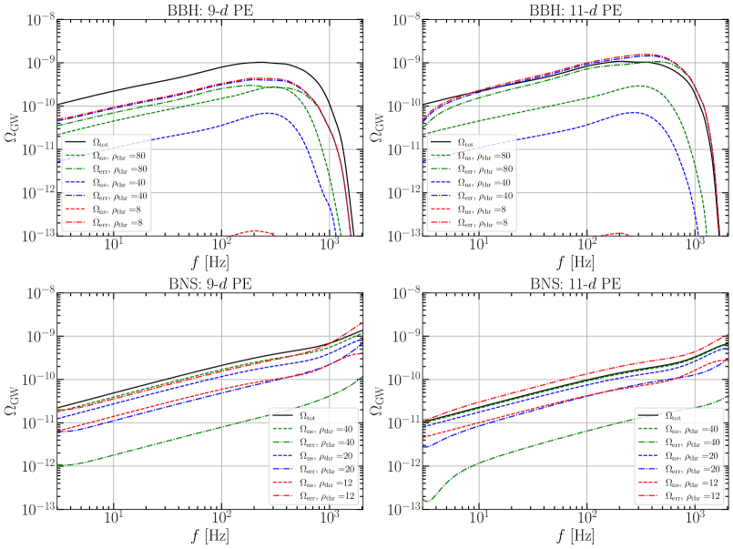
Figure 1: Results from Treatment (I) for 9-$d$ PE for BBHs (upper left) and BNSs (lower left), and 11-$d$ PE for BBHs (upper right) and BNSs (lower right). Each subfigure shows the total GW energy spectrum $\Omega_{\mathrm{tot}}$ in black solid line and two components ($\Omega_{\mathrm{ns}}$ and $\Omega_{\mathrm{err}}$) of the residual GW energy spectrum for different ${\rho}_{\rm thr}$. $\Omega_{\mathrm{ns}}$ (dash line) comes from the events that are not subtracted, while $\Omega_{\mathrm{err}}$ (dash-dotted line) comes from the imperfect subtraction of the CBC foreground. For a direct check, the two panels on the left reproduce the results of Fig. 2 in Zhou et al. (2023) for the IMRPhenomD waveform.

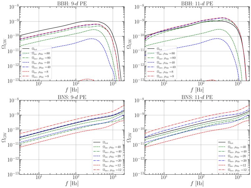
Figure 2: Same as Fig. 1, but for Treatment (II).

III Results

When we try to obtain the covariance matrix through numerical inversion, there is a condition number, $c_{\rm{\Gamma}}$, which corresponds to the accuracy of the numerical inversion of the FIM. As was pointed out by Borhanian (2021), when using GWBENCH 0.65 to calculate the covariance matrix, the inversion is not reliable if $c_{\rm{\Gamma}}$ exceeds $10^{15}$. While for the latest version 0.7.1, GWBENCH uses the mpmath routine to ensure the accuracy of numerical inversion based on the value of $c_{\rm{\Gamma}}$. Therefore, we keep all those events with a large condition number in our simulations, rather than disregarding them completely.

Due to the different treatments of events with large condition number $c_{\rm{\Gamma}}$, and for a consistency check with previous work Zhou et al. (2023), we employ two analysis treatments in the following discussion: Treatment (I) we subtract the events whose $\rho_{\rm net}>\rho_{\rm thr}$ and $c_{\rm{\Gamma}}<10^{15}$; Treatment (II) we subtract the events as long as their $\rho_{\rm net}>\rho_{\rm thr}$. Treatment (I) is consistent with the treatment in the previous version of GWBENCH which was adopted by Zhou et al. (2023), while Treatment (II) is consistent with the specifics in the version 0.7.1 of GWBENCH.

We here consider four PE cases in our calculation:

1. 9-$d$ PE for $10^{5}$ BBH events,

2. 9-$d$ PE for $10^{5}$ BNS events,

3. 11-$d$ PE for $10^{5}$ BBH events,

4. 11-$d$ PE for $10^{5}$ BNS events.

The parameter configuration of the first two cases are the same as in Zhou et al. (2023) for validation and comparison reasons. The results of these four cases from Treatment (I) are shown in Fig. 1, and from Treatment (II) are shown in Fig. 2. In each figure, the left panels show the results of 9-$d$ PE for BBH and BNS events while the right panels show the results for 11-$d$ PE cases. We denote the spectrum $\Omega_{\rm tot}$ with solid black line. Then we choose three different ${\rho}_{\rm thr}$, i.e., ${\rho}_{\rm thr}=8,40,80$ for BBH events, and ${\rho}_{\rm thr}=12,20,40$ for BNS events. For each ${\rho}_{\rm thr}$, we denote the spectrum $\Omega_{\mathrm{ns}}$ with dash line and the spectrum $\Omega_{\mathrm{err}}$ with dash-dotted line. The left panels of both figures reproduce well the results in Zhou et al. (2023), and we find similar features that $\Omega_{\mathrm{err}}$ increases with ${\rho}_{\rm thr}$ while $\Omega_{\mathrm{ns}}$ decreases with it.

However, the spectra $\Omega_{\mathrm{err}}$ in the left panels of Fig. 2 with Treatment (II) are greater than that in Zhou et al. (2023), especially for the BNS 9-$d$ PE case. This is due to the contribution from events with $c_{\rm{\Gamma}}>10^{15}$ in our Treatment (II). Those events with high $c_{\rm{\Gamma}}$ values can lead to worse subtraction results, thus contributing more to the spectrum $\Omega_{\mathrm{err}}$, comparing to the events with low $c_{\rm{\Gamma}}$ values. To see it more clearly, we define two ratios for the $i$-th event: the relative ratio $R_{\mathrm{rel}}$ and the absolute ratio $R_{\mathrm{abs}}$,

$$R_{\mathrm{rel}}=\frac{\delta h_{i}^{2}}{h_{i}^{2}},\quad\quad R_{\mathrm{abs}}=\frac{\delta h_{i}^{2}}{\overline{h^{2}}},$$ (19)

with

$$\delta h_{i}^{2} =\big{|}\tilde{h}_{+}(\bm{\theta}^{i}_{\mathrm{tr}};f)-\tilde{h}_{+}(\bm{\theta}^{i}_{\mathrm{rec}};f)\big{|}^{2}+\big{|}\tilde{h}_{\times}(\bm{\theta}^{i}_{\mathrm{tr}};f)-\tilde{h}_{\times}(\bm{\theta}^{i}_{\mathrm{rec}};f)\big{|}^{2},$$ (20)

$$h_{i}^{2} =\big{|}\tilde{h}_{+}(\bm{\theta}^{i}_{\mathrm{tr}};f)\big{|}^{2}+\big{|}\tilde{h}_{\times}(\bm{\theta}^{i}_{\mathrm{tr}};f)\big{|}^{2},$$ (21)

$$\overline{h^{2}} =\frac{1}{N}\sum_{i=1}^{N}h_{i}^{2}.$$ (22)

Notice that $\Omega_{\rm err}\propto\sum_{i=1}^{N_{s}}\delta h_{i}^{2}$ and $\Omega_{\rm tot}\propto\sum_{i=1}^{N}h_{i}^{2}$. The value of $R_{\mathrm{rel}}$ represents the ratio of an event’s contribution to $\Omega_{\mathrm{err}}$ over its contribution to $\Omega_{\mathrm{tot}}$. Considering that the value of $h_{i}^{2}$ varies from event to event, we employ $R_{\mathrm{abs}}$ to estimate the ratio of an event’s contribution to $\Omega_{\mathrm{err}}$ over the average contribution to $\Omega_{\mathrm{tot}}$ across all $N$ CBC events.

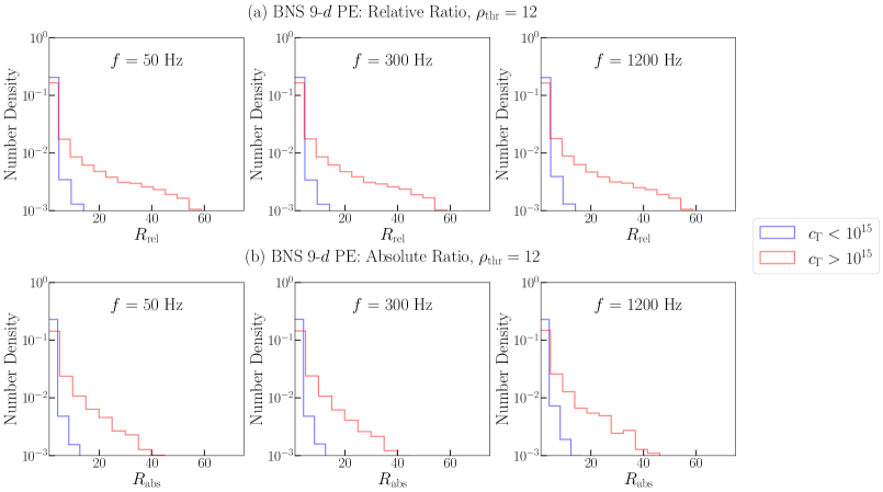
Figure 3: Number density distribution of the relative ratio $R_{\mathrm{rel}}$ (upper panels) and the absolute ratio $R_{\mathrm{abs}}$ (lower panels) for BNS 9-$d$ PE case with $\rho_{\rm thr}=12$. Plots for events with high/low $c_{\rm{\Gamma}}$ values (denoted with red/blue color) are shown separately. Three frequency bins are chosen for illustration. The distributions at 10, 100, 200, 400, 800 and 2000 Hz have similar features, which are not shown here.

Table 1: Percentage of BBH and BNS events with $c_{\rm{\Gamma}}>10^{15}$ in our simulation. For BBH cases we set $\rho_{\rm thr}=8$, while for BNS cases, we set $\rho_{\rm thr}=12$.

	9-$d$ PE	11-$d$ PE
BBH	1.76%	4.32%
BNS	21.98%	58.24%

We show the number density distribution of $R_{\mathrm{rel}}$ and $R_{\mathrm{abs}}$ for events with high and low $c_{\rm{\Gamma}}$ values separately in Fig. 3 for the BNS 9-$d$ PE case with $\rho_{\rm thr}=12$. Without loss of generality, three frequency bins are selected from low to high for illustration. We observe that events with high $c_{\rm{\Gamma}}$ values (red line) are more concentrated at higher ratio values than events with low $c_{\rm{\Gamma}}$ values (blue line) for both $R_{\mathrm{rel}}$ and $R_{\mathrm{abs}}$ at all chosen frequency bins. This indicates that events with high $c_{\rm{\Gamma}}$ values have a higher probability of resulting in a worse subtraction than events with low $c_{\rm{\Gamma}}$ values. As shown in Table 1, since there are 21.98% events with high $c_{\rm{\Gamma}}$ values for BNS events with $\rho_{\rm thr}=12$, owing to the cumulative effects of these events, we observe a larger $\Omega_{\mathrm{err}}$ in Treatment (II) compared to that in Treatment (I). Similar results are obtained for the other three PE cases. Thus, adopting Treatment (I) rather than Treatment (II) results in an underestimation of $\Omega_{\rm err}$.

Furthermore, in Fig. 4 we observe distinctive characteristics in the parameter space for events with high $c_{\rm{\Gamma}}$ values (denoted with red color), comparing to those with low $c_{\rm{\Gamma}}$ values (denoted with gray color). We set $\rho_{\rm thr}=8$ for BBH cases and $\rho_{\rm thr}=12$ for BNS cases. The major difference is that the orbital inclination angle of events with high $c_{\rm{\Gamma}}$ values is likely to be distributed close to $0$ or $\pi$. It is not surprising, since there is strong degeneracy between the parameter pairs, $\big{\{}\iota,d_{L}\big{\}}$ and $\big{\{}\psi,\phi_{c}\big{\}}$, when $\iota$ is close to $0$ or $\pi$ Cutler and Flanagan (1994); Aasi et al. (2013); Veitch et al. (2015); Usman et al. (2019). Besides, for events with high $c_{\rm{\Gamma}}$ values, the symmetric mass ratio concentrates much closer to 0.25, which means that the two masses are nearly equal.

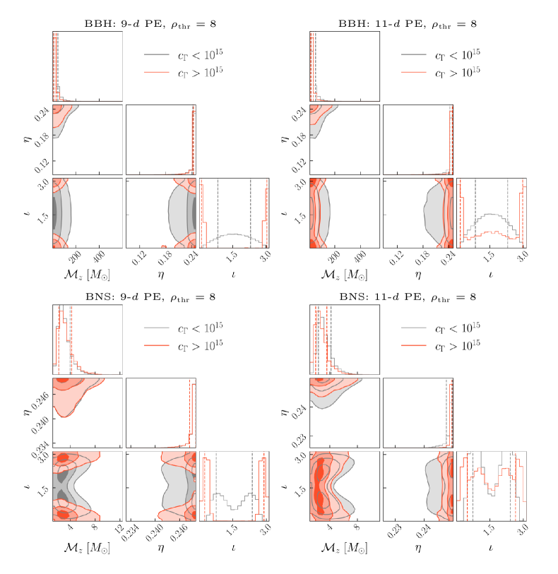
Figure 4: Parameter distributions of events with high and low $c_{\rm{\Gamma}}$ values in four PE cases. In this figure we set $\rho_{\rm thr}=8$ for BBH cases and $\rho_{\rm thr}=12$ for BNS cases. We show three parameters here: chirp mass in the observer frame $\mathcal{M}_{z}$, symmetric mass ratio $\eta$, and orbital inclination angle $\iota$. Red color denotes events with $c_{\rm{\Gamma}}>10^{15}$, while gray color denotes events with $c_{\rm{\Gamma}}<10^{15}$.

As discussed, the use of Treatment (I) underestimates $\Omega_{\rm err}$, so in the following we focus on the results of Treatment (II). As is shown in Fig. 2, when we incorporate aligned spins in PE, the spectrum $\Omega_{\rm err}$ in the right panels grow significantly, comparing to those of the 9-$d$ PE results in the left panels. This mainly comes from the degeneracy between symmetric mass ratio and spins in the waveform model at the inspiral stage Baird et al. (2013); Hannam et al. (2013); Ohme et al. (2013); Berry et al. (2015); Pürrer et al. (2016); Farr et al. (2016). As is shown in Table 2, for the BBH 11-$d$ PE case, the absolute values of the correlation coefficients $C$ among $\chi_{1z}$, $\chi_{2z}$ and $\eta$ exceed 0.99 for over 80% of all events with $\rho_{\rm thr}=8$. For the BNS 11-$d$ PE case, over 84% of all events have correlation coefficients exceeding 0.99 with $\rho_{\rm thr}=12$. The large uncertainties due to the strong degeneracy will lead to a larger spectrum of $\Omega_{\rm err}$. To see it more clearly, we follow Zhou et al. (2023) to estimate the contribution of each parameter to $\Omega_{\rm err}$. For each event, we reconstruct the waveform with the following choice of parameters. We first choose the $k$-th parameter to be drawn from the 1-$d$ Gaussian distribution with variance $\sigma_{\theta_{k}}$ (the $k$-th diagonal component of the covariance matrix $\Sigma_{\rm net}$) when using the true value as its mean $\mu_{\theta_{k}}$. Then we set all the other parameters to be their true values. Varying only one parameter and summing over all the subtracted events, we obtain $\Omega_{\rm err}$ contributed from each parameter. The results are shown in Fig. 5, where we choose ${\rho}_{\rm thr}$ equal to 8 and 12 for BBHs and BNSs separately. The contributions from $\chi_{1z}$, $\chi_{2z}$ and $\eta$ dominate the spectrum $\Omega_{\mathrm{err}}$ even at such high $\rho_{\rm thr}$ values. For the BBH case, the contribution from $\chi_{1z}$ and $\chi_{2z}$ even surpasses $\Omega_{\mathrm{err}}$ from the 11-$d$ PE results. Meanwhile, for the BNS case, there are also subdominant contributions from $D_{L}$, $\phi_{c}$, and $\mathcal{M}_{z}$. Similar results were also found by Zhou et al. (2023). As a result, the discrepancy between parameters becomes more pronounced in 11-$d$ PE cases than that in the 9-$d$ PE cases. Both the relative ratio $R_{\mathrm{rel}}$ and the absolute ratio $R_{\mathrm{abs}}$ have grown significantly, comparing to those in the 9-$d$ PE cases with $\rho_{\rm thr}=8$, which is illustrated in Fig. 6 for BBHs. Hence, we observe a larger spectrum $\Omega_{\rm err}$.

Table 2: Percentage of BBH and BNS events with the absolute values of correlation coefficients among spins and symmetric mass ratio greater than 0.99 for 11-$d$ PE cases. For the BBH case we set $\rho_{\rm thr}=8$, and for the BNS case, $\rho_{\rm thr}=12$.

	$\big{|}C_{\chi_{1z},\chi_{2z}}\big{|}>0.99$	$\big{|}C_{\eta,\chi_{1z}}\big{|}>0.99$	$\big{|}C_{\eta,\chi_{2z}}\big{|}>0.99$
BBH	98.80%	81.05%	79.98%
BNS	99.96%	84.17%	84.05%

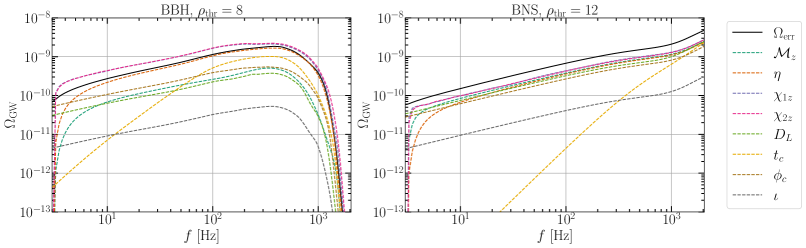
Figure 5: Contribution from each parameter to $\Omega_{\mathrm{err}}$ for BBHs (left panel) and BNSs (right panel). Each subfigure shows $\Omega_{\rm err}$ from 11-$d$ PE results (black solid line) and contribution from each parameter (dash line). We choose ${\rho}_{\rm thr}$ equal to 8 and 12 for BBHs and BNSs respectively.

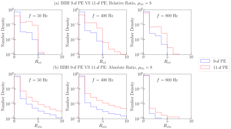
Figure 6: The relative ratio $R_{\mathrm{rel}}$ (upper panels) and absolute ratio $R_{\mathrm{rel}}$ (lower panels) for 9-$d$ PE (blue line) and 11-$d$ PE (red line) of BBHs. We set $\rho_{\rm thr}=8$ and choose 3 frequency bins to illustrate. The BNS case has a similar feature in our simulation, which is not shown here.

As was mentioned by Zhou et al. (2023), there exists a optimal $\rho_{\rm thr}$ to minimize the spectrum $\Omega_{\mathrm{res}}$ for the 9-$d$ PE cases. For the 11-$d$ PE cases, following their approach, at almost all frequency bands we find an optimal ${\rho}_{\rm thr}=373$ for BBHs and an optimal ${\rho}_{\rm thr}=200$ for BNSs to minimize the spectrum $\Omega_{\mathrm{res}}$. This implies that in our simulated populations only 612 BBH events and 7 BNS events are to be subtracted in the XG GW detector network, which is unrealistic. Therefore, a better approach is pressingly needed to deal with this issue.

IV Summary

Considering an XG detector network which includes one ET and two CEs, we estimate the possibility of detecting SGWB from non-CBC origins by subtracting the foreground from loud CBC events. To subtract the $i$-th GW event whose true waveform is $\tilde{h}^{i}_{+/\times}(\bm{\theta}^{i}_{\mathrm{tr}};f)$, we first use FIM method to approximately get the posterior distribution of the parameters. Then we randomly draw parameters $\bm{\theta}^{i}_{\mathrm{rec}}$ from this distribution to reconstruct the waveform, $\tilde{h}^{i}_{+/\times}(\bm{\theta}^{i}_{\mathrm{rec}};f)$. After subtracting the reconstructed waveform, there leaves some residual $\delta\tilde{h}^{i}_{+/\times}$ in the data [see Eq. (15)]. The summation over all the subtracted events we obtain the spectrum $\Omega_{\rm err}$, which corresponds to the energy density brought by the imperfect foreground subtraction. Then, $\Omega_{\rm err}$, combined with $\Omega_{\rm ns}$, which is the spectrum of the GW events that are not subtracted because of low SNRs, forms $\Omega_{\rm res}$. In reality we want to minimize $\Omega_{\rm res}$ so as to detect SGWB from non-CBC origins.

As an extension of the previous studies by Sachdev et al. (2020) and Zhou et al. (2023), we include spin parameters in PE, in other words, we adopt an 11-$d$ PE using the FIM for the CBC events to be subtracted. For a realistic consideration, we generate $10^{5}$ BBH and BNS events based on the latest population models provided by the LVK collaboration Abbott et al. (2023b) and consider different treatments for subtraction of events which have large condition numbers when inverting the FIM.

First, we set a threshold SNR $\rho_{\rm thr}$. For those low SNR events with $\rho_{\rm net}<\rho_{\rm thr}$, we do not subtract them since the PE uncertainties of these events are too large, and some events are even unsolvable if $\rho_{\rm net}\lesssim 8$. However, there is still no guarantee to well reconstruct the true waveform for an event with a large SNR. Sometimes, there can be strong degeneracy between some parameters in the waveform model, which leads to a large deviation between the reconstructed waveform and the true waveform. When the degeneracy between the parameters is strong, the condition number $c_{\rm{\Gamma}}$ of FIM can be very large. We propose two treatments, for Treatment (I), we subtract the events whose $\rho_{\rm net}>\rho_{\rm thr}$ and $c_{\rm{\Gamma}}<10^{15}$, and for Treatment (II), we subtract all the events as long as $\rho_{\rm net}>\rho_{\rm thr}$. Comparing the results of Treatment (I) in Fig. 1 and Treatment (II) in Fig. 2, we find significant contribution to $\Omega_{\rm err}$ from events with large $c_{\rm{\Gamma}}$. We verify it by calculating the distribution of $R_{\rm rel}$ and $R_{\rm abs}$ [see Eq. (19)], as shown in Fig. 3. To conclude, the early study underestimated $\Omega_{\rm err}$ when discarding events with large $c_{\rm{\Gamma}}$. To be more realistic, we include these events in our calculation. We also study the characteristics of the distribution of parameters when $\rho_{\rm net}>\rho_{\rm thr}$ and $c_{\rm{\Gamma}}>10^{15}$. The orbital inclination angle $\iota$ is much more likely to distribute around $0$ or $\pi$ for these events (see Fig. 4), which leads to degeneracy between $\iota$ and $D_{L}$, and $\psi$ and $\phi_{c}$. Besides, the symmetric mass ratio is more likely to be closer to 0.25 for events with high $c_{\rm{\Gamma}}$ values. By introducing higher order modes in the waveform model, we may break the degeneracy between $\iota$ and $D_{L}$, and $\psi$ and $\phi_{c}$ to some extent Lasky et al. (2016); Payne et al. (2019); Zhang et al. (2023); Gong et al. (2023), especially for the events with asymmetric masses Abbott et al. (2020a, b) or high masses Chatziioannou et al. (2019); Abbott et al. (2020c). The uncertainty in PE for events with spins can also be reduced by including non-quadrupole modes Varma et al. (2014); Calderón Bustillo et al. (2016); Varma and Ajith (2017). From this perspective, we expect to get a more optimistic result of the foreground subtraction by using a waveform model including higher order modes in the future studies.

We compare our results with those obtained by Zhou et al. (2023), where a 9-$d$ PE was adopted. After including the aligned spins, the degeneracy between parameters becomes worse, especially between the spin parameters and the symmetric mass ratio. As is shown in Fig. 5, the effects from $\chi_{1z}$, $\chi_{2z}$ and $\eta$ surpasses that from $\phi_{c}$ which dominates in the 9-$d$ PE Zhou et al. (2023). The degeneracy increases the uncertainty when performing PE and results in unexpectedly large $\Omega_{\rm res}$, which is even larger than $\Omega_{\rm tot}$.

In this work, we only consider the uncertainty of PE brought by the noise. When the error from inaccurate waveform modeling cannot be neglected Cutler and Vallisneri (2007); Gamba et al. (2021); Pürrer and Haster (2020); Hu and Veitch (2023), it also needs to be discussed quantitatively in future study. Last but not least, we have assumed that GW signals can be identified and then subtracted one by one in the literature. However, it seems very optimistic for XG detectors, since there can be plenty of GW signals overlapping with each other, making PE more difficult Regimbau et al. (2012); Meacher et al. (2016); Samajdar et al. (2021); Pizzati et al. (2022); Relton and Raymond (2021); Wang et al. (2023); Dang et al. (2023). We have to take into account the effects of overlapping between signals in future studies.