Automated Model Selection for Tabular Data

Abstract

Structured data in the form of tabular datasets contain features that are distinct and discrete, with varying individual and relative importances to the target. Combinations of one or more features may be more predictive and meaningful than simple individual feature contributions. R’s mixed effect linear models library allows users to provide such interactive feature combinations in the model design. However, given many features and possible interactions to select from, model selection becomes an exponentially difficult task. We aim to automate the model selection process for predictions on tabular datasets incorporating feature interactions while keeping computational costs small. The framework includes two distinct approaches for feature selection: a Priority-based Random Grid Search and a Greedy Search method. The Priority-based approach efficiently explores feature combinations using prior probabilities to guide the search. The Greedy method builds the solution iteratively by adding or removing features based on their impact. Experiments on synthetic demonstrate the ability to effectively capture predictive feature combinations. Code is available at .

1 Introduction

Machine learning methods have been greatly useful at mechanising the process of dealing with input data with a large number of features. Unlike image and vision datasets, where all input components are of a similar kind and equally important, tabular datasets contain data structured into categories and continuous variables, organised into rows and columns. These datasets find applications across diverse domains, including but not limited to finance, healthcare, e-commerce. The features available in these datasets are discrete and distinct in their contributions and cannot be treated simplistically as alike unlike image/text datasets.

Feature interactions occur when the combination of two or more features provides insights and information that cannot be derived from considering each feature in isolation. For example, the Adult Income dataset [Dua et al., 2019] contains features like education-level, marital-status, race, gender etc., which are not equally important to income and are related in ways that might in some combinations, strongly predict income when together than treated separately. For example, it is possible that when gender=female and marital-status=married and age $\in$ 25-35 the combination of these factors would indicate a higher likelihood of child-bearing and maternity leave which would have a significant effect on one’s income compared to combining these indicators’ contribution individually: because of the way the features interact. Thus, in this context of classification and regression on such tabular data, the choice of features used plays a pivotal role in the performance of our predictors. The role of feature interactions within tabular datasets has received increasing attention in recent years in works like [Xie et al., 2020] and [Liu et al., 2020]. Linear Regression (LR) models linearly aggregate features without modeling complex feature interactions. This can limit performance when interdependencies exist. Recognizing and effectively modeling feature interactions is pivotal in enhancing the overall performance and interpretability of models.

Our work entails investigating tabular feature interactions and developing two distinct approaches for feature selection: Priority-based Random Grid Search and Greedy Search methods. We created a synthetic dataset that included categorical variables like age, education, work status, and country codes, along with interactions for marital status and gender features. A Priority-based Random Grid Search algorithm, designed for efficient exploration of feature combinations, incorporated prior probabilities to streamline the process. Greedy approach was also evaluated where we built our solution feature set iteratively. We assess feature interactions systematically while keeping in mind the computational demands.

2 Related works

[Xie et al., 2020] introduces a framework FIVES: Feature Interaction Via Edge Search, This method involves searching for meaningful interactions among features by formulating it as a edge search over the feature graph GNN. [Shekar et al., 2017] proposed a filter-based framework to assess features, known as Relevance and Redundancy (RaR) to incorporate multiple interactions among features and to account for redundancy in ranking features within mixed datasets. RaR generates a single score for assessing the relevance of features by taking into consideration feature interactions and redundancy. On the other hand, [Qin et al., 2021] introduces the Retrieval $\&$ Interaction Machine (RIM) framework for predicting outcomes in tabular data, emphasizing both cross-row and cross-column patterns. RIM leverages search engine techniques to efficiently retrieve relevant rows and utilizes feature interaction networks for enhanced label predictions. Extensive experiments across various tasks demonstrate RIM’s superiority over existing models and baselines, highlighting its effectiveness in improving prediction performance.

XDeepFM [Lian et al., 2018] adds explicit feature-product calculations to the model architecture to exploit feature interactions to improve recommender systems. They introduced the Compressed Interaction Network (CIN), which generates explicit and vector-wise feature interactions. The proposed eXtreme Deep Factorization Machine (xDeepFM) unifies CIN and DNN to learn bounded-degree and arbitrary feature interactions. [Zeng et al., 2015] introduced an interaction weight factor designed to convey whether a feature exhibits redundancy or interactivity and use this in feature selection. Though these papers do involve the idea of feature interactions, they are not applicable as baselines to our setting. This is because FIVES works with complex models on graph GNNs and XDeepFM is specific to recommender systems. In addition to this, while our task is about trying different feature combinations and automating selections from these, these works do not explore these aspects and are content with incorporating feature interactions into their respective problem setting.

3 Background and hypotheses

3.1 Background

Feature selection: Feature selection is a process of automatically choosing the relevant features by including relevant features or excluding irrelevant features. The aim is to enhance model efficiency and mitigate overfitting. Various strategies exist for feature selection, ranging from filter methods such as Information gain, chi-squared test that assess individual feature relevance, wrapper methods such as forward selection, backwards elimination, exhaustive feature selection that leverage model performance, to embedded methods such as regularization where feature selection is integrated into the model training process.

Feature-relevance: [Zhao and Liu, 2009] defines that a feature is relevant only when its removal from a feature set will reduce the output confidence on a class. Let $F$ be the full set of features, and $F_{i}$ be a feature, define the set $S_{i}=F-{F_{i}}$ and $P$ denote the conditional probability of class C given a feature set. A feature $F_{i}$ is relevant iff $\exists S^{\prime}_{i}\subseteq S_{i}$, such that $Pr(C|F_{i},S^{\prime}_{i})\neq Pr(C|S^{\prime}_{i})$. Otherwise, the feature $F_{i}$ is irrelevant.

$k^{th}$ order feature interactions: [Zhao and Liu, 2009] defines the k the order feature interactions as follows. Let $F$ be a feature subset with $k$ features $F_{1},F_{2},...,F_{k}$. Let $\zeta$ denote a metric that measures the relevance of the class label with a feature or a feature subset. We say features $F_{1},F_{2},...,F_{k}$ are said to interact with each other iff for an arbitrary partition $\mathcal{F}=\{\mathcal{F}_{1},\mathcal{F}_{2},\mathcal{F}_{3},...,\mathcal{F}_{l}\}$ of $F$, where $l\geq 2$ and $\mathcal{F}_{i}\neq\phi$, we have $\zeta(F)>\zeta(\mathcal{F}_{i})$ $\forall$ $i\in[1,l]$

Explicit vs implicit feature capturing: Complex models like neural networks and ensembles can implicitly capture feature interactions. This means that these models automatically learn and consider relationships between features without explicitly modeling them. While this enables powerful predictive capabilities, it often leads to a lack of explainability. Understanding how and why these models make specific predictions can be challenging due to the intricate and implicit nature of feature interactions within these models.

In this work, we avoid the lack of explainability caused by implicit feature interactions while relying on complex models. We use linear models to explicitly model feature interactions. Linear models are inherently more interpretable, making them suitable for capturing and explaining feature relationships in a straightforward manner. We can harness the strengths of complex models for prediction while providing transparent insights into the relationships between features, ultimately yielding more explainable and trustworthy models.

3.2 Objective and Framework

We aim to solve the feature selection problem in the specific context of tabular datasets (that have categorical features) and where many of the features we search over are interaction features formed by crossing the base features. (Note that we treat categorical values as one-hot encoded which can be crossed by set-cross product). We hypothesize that tabular datasets have features which interact in predictive manners. These interactions are not exploited with simple linear models that just add up individual base feature contributions. In addition, the space of the possible feature interactions would be too large to explore with a grid search or random search in terms of computational costs.

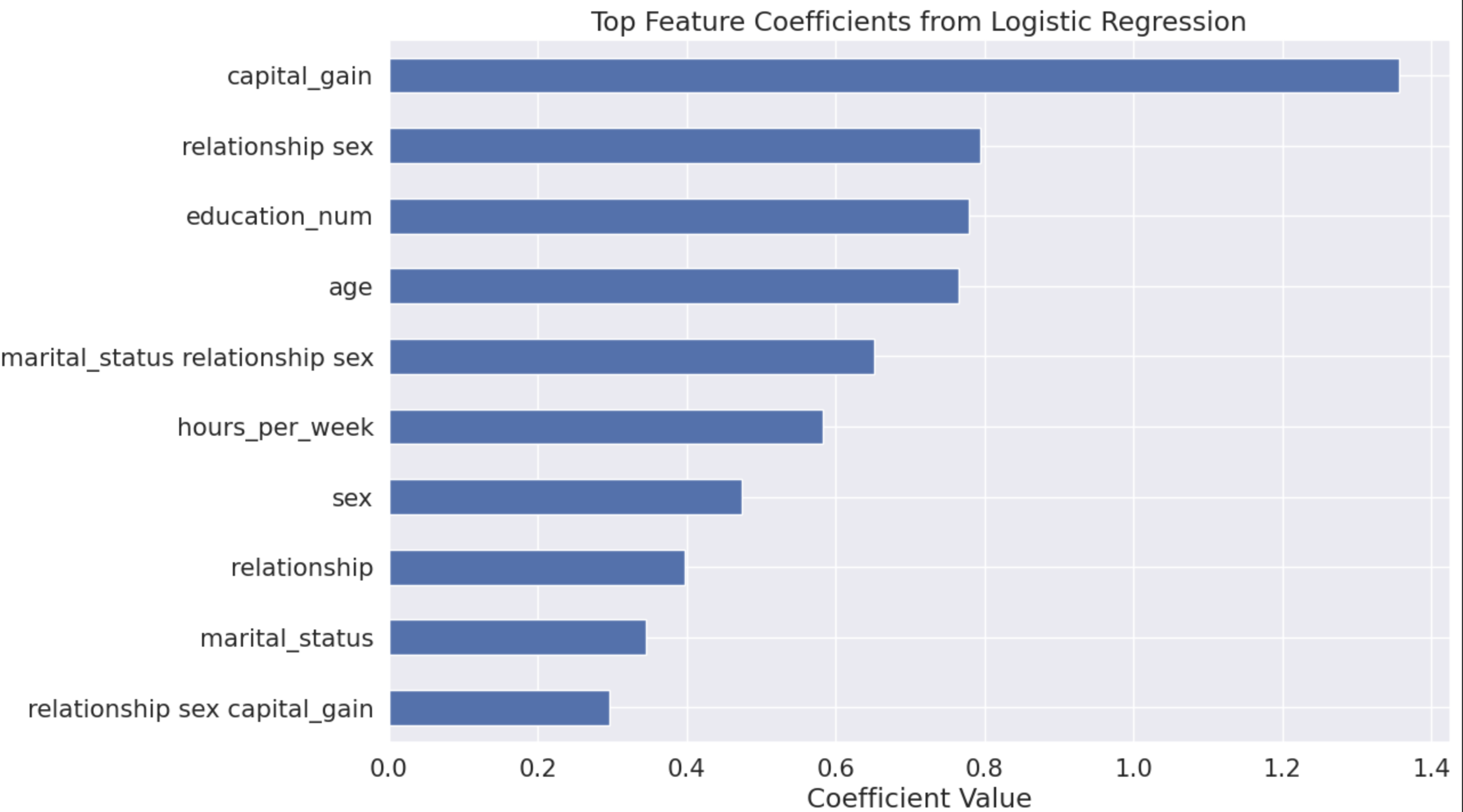
Figure 1: Feature importances in the real-life Adult Income dataset.

We see the potential for automating this search for an optimum model, while keeping computational costs small. We will optimise our search using prior assumptions on the extent of feature interactions and using feature importances to cut our search space short. At the milestone stage, we have implemented priors on feature interactions, and in next steps will incorporate prioritising individual feature importances in our search.

We plan to optimize the metrics of the model such as $R^{2}$ value (coefficient of determination), MSE (mean squared error), Log-likelihood and AIC (Akaike Information Criterion) to show the performance of our models. We also track runtime of feature search to evaluate computational efficiency of the search. The main libraries we use are from various sklearn, numpy, statsmodels and pandas functionalities. We work with linear regression models applied on categorical variables. For this we apply sklearn’s LinearRegression functionality upon various one-hot encoded Python pandas dataframes. We also plan to explore generalized models and ensemble models. We encode categorical features using one-hot encoding before fitting linear regression models.

4 Data

4.1 US Adult Income dataset and discussion

We conducted experiments on the US Adult Income dataset [Dua et al., 2019], aiming to predict income levels (above or below $50k$) using details about the person such as their age, education, occupation status, race, gender etc. Our focus was on assessing the impact of feature interactions on model performance. The pipeline integrated sklearn’s PolynomialFeatures module to generate interaction terms and a Logistic Regression classifier, coupled with hyperparameter tuning via grid search.

Grid search on Adult Income Data: We use Sklearn’s PolynomialFeatures module with the interactions_only parameter set to true, eliminating squared terms. GridSearchCV optimized the logistic regression model, considering interactions via PolynomialFeatures. The search spanned various degrees of polynomial features, ensuring the selection of the optimal model variant in terms of accuracy, balancing complexity with predictive power. Post GridSearchCV, ‘capital_gain’ emerged as the most significant predictor. Notable interaction terms included ‘relationship-sex’ and ‘maritalstatus-relationship-sex’, highlighting their relevance. The feature importance plot is depicted in Figure 1.

This interaction-based model achieved a test accuracy of 0.7911, while the original linear model (trained without interactions) yielded a test accuracy of 0.817 for Logistic Regression. If interactions in the dataset were significant, we would expect higher accuracy with our interaction-based model. We thus hypothesize that our assumption of significant interactions in this real-life dataset did not hold true.

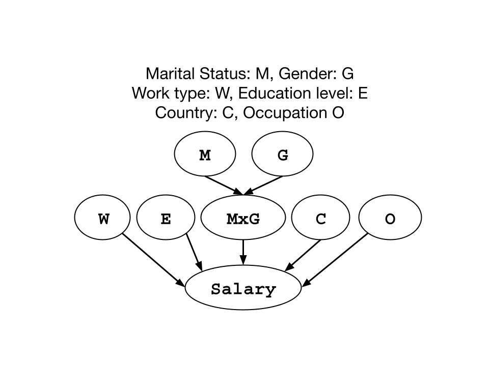
Figure 2: Causal diagram showing the interactions between the features used to create the synthetic dataset.

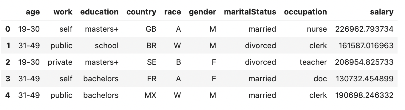
Figure 3: A snippet of the generated synthetic dataset Adult2.

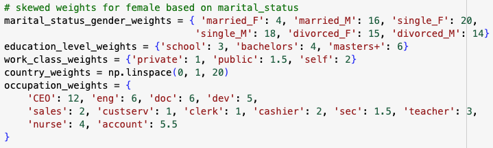
Figure 4: Weight assignment in Adult2 creation

4.2 Synthetic data generation

Based on the above analysis on the Adult dataset, we fell back to creating a synthetic dataset where we incorporate some desired feature interactions. These feature interactions serve as the ground truth to evaluate our method on. We generated a synthetic dataset we call ‘Adult2’, deliberately incorporating feature interactions. We assigned weights to the features and combinations of features as illustrated in figure 4. These weights were then used to combine the contributions of the features into the target (label) attribute, salary.

Formally, let $F$ be the full set of features and $F_{I}\subseteq F$ be the subset of features with 2nd order features (interactions) i.e., $F_{I}=\{(F_{i},F_{j})\}$ where $F_{i},F_{j}$ are the features with interactions. Define $F^{\prime}=F-F_{I}$ (to avoid features being redundant by appearing both in first and second order forms). We define true label $y=f(F^{\prime},F_{I})$. In the above example, we take the function $f$ to be linear.

The core of our dataset creation process is our self-assigned weights (figure 4) for each of the ground truth model’s features. We convert the given data’s feature set into a final feature set by crossing-among and selecting features. We then add up their individual contributions to create our target column. Note: incorporation of feature interactions into our dataset generation above is done by assigning weights to crossed-feature combinations - which we call our interaction features. These interaction features would be non-linear in terms of the individual components. Our dataset has categorical features such as ‘Age’, ‘Work’, ‘Education’, ‘Country’, ‘Race’, ‘Gender’, ‘MaritalStatus’, and ‘Occupation’. In the data generation phase, we assign weights to these features and combinations of these features, so as to combine their contributions into the target (label) attribute - salary.

We generate data attributes by uniform random generation over the possible value space. In our setting, we introduced interactions via a designed feature, ‘MaritalStatusGender’ to capture the interaction between ‘MaritalStatus’ and ‘Gender’. We set the weights for this feature so that it is not linear in terms of the individual components (see fig. 4). This feature, along with a subset of base features is weighted and added up to generate our target attribute ‘Salary’. This process is illustrated in figure 2. Let all the features used be called ($F_{used}$). At the end, to introduce variability, we inject a noise factor to Salary, creating a 2000 sample dataset. A snippet from this dataset is displayed in figure 3.

Data Analysis: We conducted training on two linear regression models using different datasets. The first model, trained on the raw data (X, y) using just the first order features ($F$) provided directly without interactions, yielded an $R^{2}$ value of 0.70. We then sanity-checked our interaction generation by manually creating a second model, which uses the same features and interactions as the true hidden model ($F_{used}$) we used to create the data. This model achieved a 0.9957 $R^{2}$ score showing the effectiveness of an interaction based feature set.

This shows that these features without interactions are not sufficient to explain the dataset variance under a linear model: we needed to explore the crossed-feature interactions to get the full performance. Thus in our dataset, the target/true label y is better explained as a function of input feature interactions than features without interactions.

5 Techniques and methods

5.1 Priority-based random grid search

Initially, we considered a full grid search, exploring nearly $2^{n+{n\choose 2}+{n\choose 3}+...+{n\choose n}}$ potential combinations of features and interactions, where n represents the number of features in the dataset, and ${n\choose r}$ represents the interactions of degree r. Due to the computational complexity and substantial computation time associated with all these possibilities, we decided to restrict to exploring interactions only via the second order. This still leaves $2^{n+{n\choose 2}}$ possible feature subsets involving the base features and the 1st order interaction features. So we had to simplify it further by assuming that there would be very few feature interactions among the ${n\choose 2}$ combinations involved in the true model. We took the number of 2nd order feature interaction terms as being [0, 1, 2].

Algorithm 1 Priority based random grid search

1:$D$ (dataset with $n$ features), $N$ (number of iterations)

2:Let $F=\{f_{1},f_{2},...,f_{n}\}$ (base features)

3:Let $I=\{f_{jk}|1\leq j<k\leq n\}$ (2^nd order interaction features)

4:Init: $F_{\text{best}}\leftarrow\emptyset$, $R_{\text{best}}\leftarrow 0$.

5:for $iteration=1$ to $N$ do

6:     Sample $k\sim\text{Prior}(k)$, for #interactions

7:     Sample $I_{\text{selected}}\subset I$, where $|I_{\text{selected}}|=k$

8:     Sample $F_{\text{sampled}}\subset F$, ensuring already selected interaction features are excluded.

9:     $F_{\text{cur}}=F_{\text{sampled}}\cup I_{\text{selected}}$

10:     Build LR linear model($F_{\text{cur}}$), train for $R^{2}$ score $R_{\text{cur}}$

11:     if $R_{\text{cur}}>R_{\text{best}}$ then

12:         $F_{\text{best}}=F_{\text{current}}$, $R_{\text{best}}=R_{\text{cur}}$

13:     end if

14:end for

15:return $F_{\text{best}}$

Thus our feature selection process (refer algorithm 1) could be done via separate selections over the base and interaction feature set spaces: 1. A small number k from the ${n\choose 2}$ combinations’ set and 2. Most of the features from the base feature columns. For 1., we first sample k, using assigned prior probabilities on k ranging from 0 to 2. Then these k interaction features are randomly sampled following the prior distribution from the combination set. To ensure that there exist no redundancy in the features among both the selections and we remove the features that are in the sampled interaction feature set (first selection set) from the overall base features before sampling the set of features without interaction. In 2., base feature set is randomly sampled from the remaining features. The three sections italicized above are the priors we have imposed on our search to make it simpler and easier, in contrast to a naive brute-force grid search over features. We expect these priors to give us decent results with lesser number of iterations.

In summary, our priority search approach divides the naive random grid search into separate prior-based grid searches across base features and interaction features to better reach the optimum feature set.

Algorithm 2 Backward Elimination

1:Dataset $D$ (X,y), Significance level $\alpha$

2:Encode categorical features of $X$ including 2nd-order interactions into n One-Hot features

3:Init: $F_{\text{selected}}\leftarrow\{f_{1},f_{2},...,f_{n}\}$

4:Fit a linear model with ($F_{\text{selected}},y$) ans store p-values and std error for all features

5:$pvalue_{\text{max}}\leftarrow$ maximum p-value

6:while $pvalue_{\text{max}}>\alpha$ do

7:     $f_{\text{worst}}\leftarrow$ feature with highest p-value and standard error

8:     Remove $f_{\text{worst}}$ from $F_{\text{selected}}$

9:     Fit a linear model with ($F_{\text{selected}},y$) and store p-values and std error for all features

10:     $pvalue_{\text{max}}\leftarrow$ maximum p-value

11:     if abrupt increase in AIC then

12:         break

13:     end if

14:end while

15:return $F_{\text{selected}}$

Algorithm 3 Forward Selection

1:Dataset $D$ (X,y), Significance level $\alpha$

2:Encode categorical features of $X$ including 2nd-order interactions into n One-Hot features

3:Let $F=\{f_{1},f_{2},...,f_{n}\}$ (individual features)

4:Init: $F_{\text{selected}}\leftarrow\emptyset$

5:$pvalue_{\text{min}}\leftarrow$ -$\infty$

6:while $pvalue_{\text{min}}<\alpha$ do

7:     Fit a linear model with ($F_{\text{selected}}\cup f_{i},y$). Repeat this $\forall$ $f_{i}\in F$, and store {$f_{i}$: (pvalue for feature $F_{i}$ , std error for feature $F_{i}$ )} across all the models

8:     $f_{\text{best}}\leftarrow$ feature with minimal p-value and std error

9:     $pvalue_{\text{min}}\leftarrow$ minimal p-value

10:     Add $f_{\text{best}}$ to $F_{\text{selected}}$

11:     Remove $f_{\text{best}}$ from $F$

12:     if abrupt increase in AIC then

13:         break

14:     end if

15:end while

16:return $F_{\text{selected}}$

5.2 Greedy search

We explore the approaches to feature selection using a greedy strategy. Greedy search is a heuristic optimization strategy that makes locally optimal choices at each step with the hope of finding a global optimum. In the context of feature selection in machine learning, greedy search involves iteratively making decisions to add or remove features based on their immediate impact, aiming to improve the overall model performance. Backward Elimination and Forward Selection are two variants of greedy search used for feature selection.

Backward Elimination: Described in algorithm 2, this top down approach involves fitting the model with all possible features initially, considering both interactions and individual features. It then iteratively removes the least important features, narrowing down the feature set for optimal model performance. To identify features that have a lesser impact on the model, our strategy involves assessing p-values, and standard errors with respect to each feature. The feature with higher p-value and standard error with respect to the fitted linear model are removed. Since our data contains only categorical features we apply one hot encoding before fitting the model.

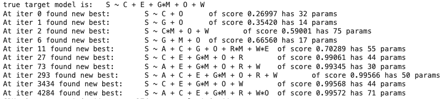
Figure 5: Evolution of the best feature set over iterations of the priority search algorithm. From the figure, we observe that the true model is found after 3483 iterations

Forward Selection: Described in algorithm 3, this bottom-up approach entails creating individual simple regression models for each feature in the dataset. p-values and standard errors are then calculated for these models, and the feature with the lowest p-value and standard error is selected. This chosen feature is added to models of other features, resulting in one less linear regression model, but each of them will have two features. Continue iterating the approach keeping track of the selected features until the lowest p-value from a model is no longer below the significance level, typically $\alpha$ = 0.01 . This approach refines the model by gradually including features with significant contributions.

6 Results

6.1 Priority-based random grid search

Figure 5 shows our result for priority search. We observe that the true model is captured at iteration 3434. The better scoring model found later is overfit with more parameters (a superset of the already found true model), both have the almost same score. We also achieve full 99.6% accuracy (because the synthetic data was made using the same linear additions we capture in our LR models).

The following graph (Figure 6) depicts the $R^{2}$ value of the best model identified in relation to the number of times the algorithm was executed. On average, the peak performance of the best model is observed around the $3434^{th}$ iteration. Total iterations for all possible feature subsets for our dataset (under highest degree of interaction being 2) would’ve been $2^{8+{8\choose 2}}$.

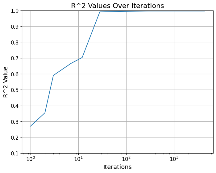
Figure 6: Best performance achieved ($R^{2}$) vs N with the priority search algorithm.

6.2 Greedy Search

Considering the 8 base features in the synthetic data (Figure 3), and the 2nd order interactions features (28), there are 36 features and the potential feature space after one-hot encoding is 953 (coefficients). This results in a total of $2^{953}$ feature subsets, making it computationally intensive to find the best model. Thus we use greedy approach to optimize the search space. Figure 7, 8 shows the learning curve for Forward selection algorithm and backward elimination respectively considering the metrics $R^{2}$, MSE, AIC, Log-likelihood.

6.3 Discussion

Table 1 summarizes the results from priority search, backward elimination and forward selection. From the table 1, we can conclude that the optimal solution using forward selection and backward elimination may differ.

For the synthetic dataset we performed all the above mentioned methods and observed the following results:

1. Random Priority search achieved a 99.57% $R^{2}$ with an average runtime of 2 to 3 minutes, capturing a near-optimal (near true) model. This method required fewer iterations and took less time.

2. The Forward selection achieved a 99.62% $R^{2}$ on the synthetic data with an average runtime of 20 to 30 minutes, capturing the true model.

3. The Backward Selection achieved over 99.68% $R^{2}$ with an average runtime of 10 to 15 minutes, capturing a near-optimal solution.

From the experiments, the forward selection seems to give us the true model when compared to the other approaches. Priority based random grid search required the fewer iterations and runtime when compared with the other greedy approaches. This highlights a tradeoff between computational efficiency and performance. Importantly, all methods outperformed baseline linear models, demonstrating the value of modeling feature interactions.

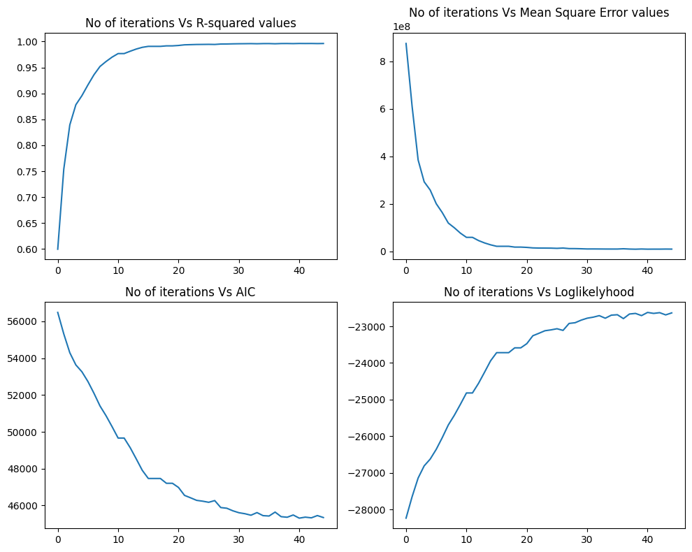
Figure 7: Forward Selection performance. We terminated forward selection when the p-value of the added feature increased beyond 0.01, which implies that an insignificant feature has been added.

Algorithm	Priority based-random grid search	Forward Selection	Backward Elimination
Obtained Model	S $\sim$ A + C + E + M*G + O + W*R	S $\sim$ C + E + M*G + O + W	S $\sim$ A*R + C*O + E + M*G + W
Avg. runtime on colab	1-3 min	20-30 min	10-15 min
$R^{2}$	0.9957	0.9962	0.9968
MSE	9.59e6	8.83e6	1.09e7
AIC	3.02e4	4.53e4	4.57e4
Log-Likelihood	-1.5e4	-2.26e4	-2.24e4

Table 1: Comparing priority search, backward elimination and forward selection statistics. We also report the generated model against the true model, which is S $\sim$ C + E + M*G + O + W.

7 Conclusion

In this work, we investigated automated model selection incorporating feature interactions for tabular datasets. We hypothesized that combinations of features can be more predictive than individual contributions. We proposed three approaches: a Priority-based Random Grid Search, a Greedy Search method with forward selection, and backward elimination. The Priority search uses priors to efficiently explore feature subsets. The Greedy approach iteratively adds/removes features based on impact. Experiments conducted on real world Adult dataset reveals that there are no singificant interactions hence we fall back to create synthetic dataset on which forward selection algorithms achieves true model whereas priority-based random grid search achieves near optimal model with minimal computational time.

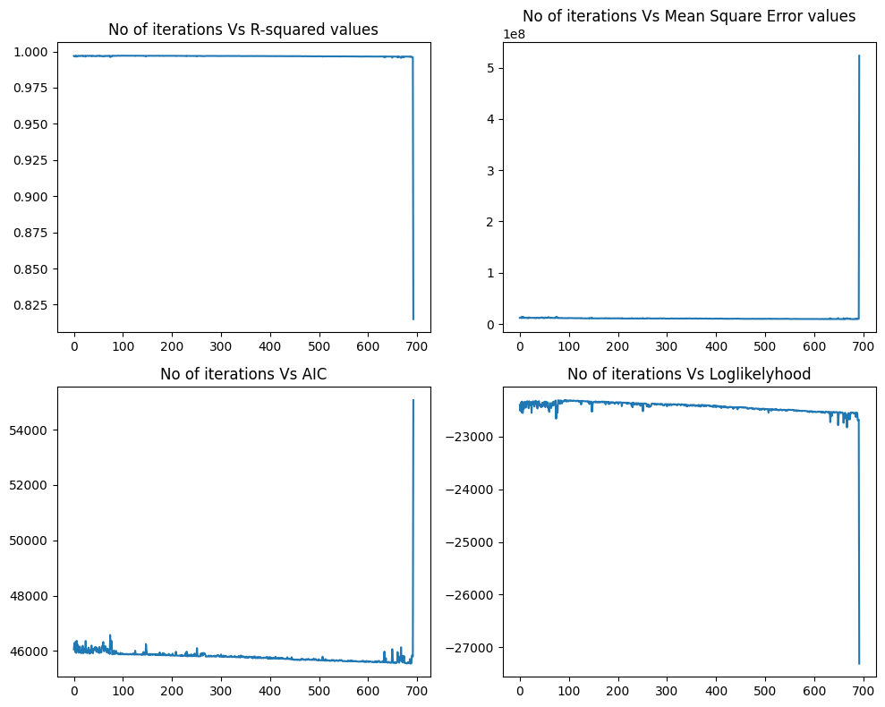
Figure 8: Backward Elimination performance. We terminate backward elimination due to sudden surge in AIC, which implies that a crucial features has been removed.

8 Future work

The first area of improvement involves refining the Priority based Random Grid search by incorporating a learned prior probability distribution on k. Additionally, expanding the size of k and implementing downweighting based on feature size is planned, with the aim of addressing large feature spaces such as country x occupation, which may result in a substantial number of possible values. Another avenue for improvement is the optimization of the Greedy algorithm by considering H-statistics. The exploration of various regularization methods for feature selection is also slated for investigation. Lastly, a comparative SHAP analysis between forward selection and backward elimination will be conducted to gain insights into the interpretability and impact of these feature selection approaches. These proposed enhancements collectively aim to advance the effectiveness and efficiency of the current research methodology.

References

- [Dua et al., 2019] Dua, D., Graff, C., et al. (2019). Uci machine learning repository, 2017. URL http://archive. ics. uci. edu/ml, 7(1).
- [Lian et al., 2018] Lian, J., Zhou, X., Zhang, F., Chen, Z., Xie, X., and Sun, G. (2018). xdeepfm: Combining explicit and implicit feature interactions for recommender systems. CoRR, abs/1803.05170.
- [Liu et al., 2020] Liu, Z., Liu, Q., Zhang, H., and Chen, Y. (2020). DNN2LR: interpretation-inspired feature crossing for real-world tabular data. CoRR, abs/2008.09775.
- [Qin et al., 2021] Qin, J., Zhang, W., Su, R., Liu, Z., Liu, W., Tang, R., He, X., and Yu, Y. (2021). Retrieval & interaction machine for tabular data prediction. In Proceedings of the 27th ACM SIGKDD Conference on Knowledge Discovery & Data Mining, KDD ’21, page 1379–1389, New York, NY, USA. Association for Computing Machinery.
- [Shekar et al., 2017] Shekar, A., Bocklisch, T., Sánchez, P., Straehle, C., and Müller, E. (2017). Including Multi-feature Interactions and Redundancy for Feature Ranking in Mixed Datasets, pages 239–255.
- [Xie et al., 2020] Xie, Y., Wang, Z., Li, Y., Ding, B., Gürel, N. M., Zhang, C., Huang, M., Lin, W., and Zhou, J. (2020). Interactive feature generation via learning adjacency tensor of feature graph. CoRR, abs/2007.14573.
- [Zeng et al., 2015] Zeng, Z., Zhang, H., Zhang, R., and Yin, C. (2015). A novel feature selection method considering feature interaction. Pattern Recognition, 48(8):2656–2666.
- [Zhao and Liu, 2009] Zhao, Z. and Liu, H. (2009). Searching for interacting features in subset selection. Intelligent Data Analysis, 13(2):207–228.