The Rank of the Odd Normal Out

Abstract

Say we have a collection of independent random variables $X_{0},\ldots,X_{n}$, where $X_{0}\sim\mathcal{N}\left(\mu_{0},\sigma_{0}^{2}\right)$, but $X_{i}\sim\mathcal{N}\left(\mu,\sigma^{2}\right)$, for $1\leq i\leq n$. We characterize the distribution of $R_{0}\coloneqq 1+\sum_{i=1}^{n}\mathbf{1}_{\left\{X_{i}\leq X_{0}\right\}}$, the rank of the random variable whose distribution potentially differs from that of the others—the odd normal out. We show that $R_{0}-1$ is approximately beta-binomial, an approximation that becomes equality as $\nicefrac{{\sigma}}{{\sigma_{0}}}$ or $\nicefrac{{\left(\mu-\mu_{0}\right)}}{{\sigma_{0}}}$ become large or small. The intra-class correlation of the approximating beta-binomial depends on $\Pr\left(X_{1}\leq X_{0}\right)$ and $\Pr\left(X_{1}\leq X_{0},X_{2}\leq X_{0}\right)$. Our approach relies on the conjugacy of the beta distribution for the binomial: $\Phi\left(\nicefrac{{\left(X_{0}-\mu\right)}}{{\sigma}}\right)$ is approximately $\mathrm{Beta}\left(\alpha\left(\nicefrac{{\sigma}}{{\sigma_{0}}},\nicefrac{{\left(\mu-\mu_{0}\right)}}{{\sigma_{0}}}\right),\beta\left(\nicefrac{{\sigma}}{{\sigma_{0}}},\nicefrac{{\left(\mu-\mu_{0}\right)}}{{\sigma_{0}}}\right)\right)$ for functions $\alpha,\beta>0$. We study the distributions of the in-normal ranks. Throughout, simulations corroborate the formulae we derive.

1 Introduction

With $X_{0}\sim\mathcal{N}\left(\mu_{0},\sigma_{0}^{2}\right)$ and, independently, $X_{1},X_{2},\ldots,X_{n}\stackrel{{\scriptstyle\mathrm{iid}}}{{\sim}}\mathcal{N}\left(\mu,\sigma^{2}\right)$, we would like to know the distribution of

$$R_{0}\coloneqq 1+\sum_{i=1}^{n}\mathbf{1}_{\left\{X_{i}\leq X_{0}\right\}}$$ (1)

That is, we would like to know the distribution of the rank of the normal random variable whose distribution (typically) differs from that of the others. How—in particular—does $\mathscr{L}\left(R_{0}\right)$ depend on $\mu_{0},\mu\in\mathbb{R}$; $\sigma_{0},\sigma\in\left(0,\infty\right)$; and $n\geq 1$? We predict that: if $\mu_{0}\ll\mu$, then $R_{0}\approx 1$; if $\mu_{0}\gg\mu$, then $R_{0}\approx n+1$; if $\sigma_{0}\ll\sigma$, then $R_{0}\approx 1+\nicefrac{{n}}{{2}}$; and, if $\sigma_{0}\gg\sigma$, then $\left|R_{0}-1-\nicefrac{{n}}{{2}}\right|\approx\nicefrac{{n}}{{2}}$.

We first note that

$$\left(R_{0}\left|X_{0}\right.\right)\sim 1+\mathrm{Binomial}\left(n,\Phi\left(\frac{X_{0}-\mu}{\sigma}\right)\right)$$ (2)

for $\Phi\left(x\right)$ the cumulative distribution function (CDF) of the standard normal distribution. We then have

$$\Pr\left(R_{0}=k\right)=\binom{n}{k-1}\mathbb{E}\left[\Phi\left(\frac{X_{0}-\mu}{\sigma}\right)^{k-1}\Phi\left(\frac{\mu-X_{0}}{\sigma}\right)^{n+1-k}\right]$$ (3)

for $1\leq k\leq n+1$. With the expectation in (3) looking impossible to compute, we instead take the following tack. We relate the distribution of $\Phi\left(\left.\left(X_{0}-\mu\right)\right/\sigma\right)$ to a particular beta distribution and then use its conjugacy with the binomial to obtain a closed-form approximation to (3).

What is the distribution of $\Phi\left(\left.\left(X_{0}-\mu\right)\right/\sigma\right)$? Fixing $y\in\left(0,1\right)$ we have

$$\Pr\left(\Phi\left(\frac{X_{0}-\mu}{\sigma}\right)\leq y\right) =\Pr\left(\frac{X_{0}-\mu_{0}}{\sigma_{0}}\leq\frac{\mu-\mu_{0}}{\sigma_{0}}+\frac{\sigma}{\sigma_{0}}\Phi^{-1}\left(y\right)\right)$$ (4)

$$\eqqcolon\Pr\left(\frac{X_{0}-\mu_{0}}{\sigma_{0}}\leq\delta+\rho\Phi^{-1}\left(y\right)\right)$$ (5)

$$=\Phi\left(\delta+\rho\Phi^{-1}\left(y\right)\right)\eqqcolon F_{\rho,\delta}\left(y\right)$$ (6)

where $\Phi^{-1}$ gives the inverse standard normal CDF, $\delta\coloneqq\frac{\mu-\mu_{0}}{\sigma_{0}}\in\mathbb{R}$ standardizes the mean of $X_{1},X_{2},\ldots,X_{n}$ using the mean and standard deviation of $X_{0}$, and $\rho\coloneqq\nicefrac{{\sigma}}{{\sigma_{0}}}\in\left(0,\infty\right)$ gives the ratio of the two standard deviations. While $\delta$ and $\rho$ completely characterize the distribution of $\Phi\left(\left.\left(X_{0}-\mu\right)\right/\sigma\right)$, we rely on them in what follows. Note that, if $\delta=0$ and $\rho=1$ (i.e., if $\mu=\mu_{0}$ and $\sigma=\sigma_{0}$), then $\Phi\left(\left.\left(X_{0}-\mu\right)\right/\sigma\right)$ is uniform on $\left(0,1\right)$. We further note that $\Phi\left(\left.\left(X_{0}-\mu\right)\right/\sigma\right)$ has density function

$$f_{\rho,\delta}\left(y\right)\coloneqq\rho\left.\phi\left(\delta+\rho\Phi^{-1}\left(y\right)\right)\right/\phi\left(\Phi^{-1}\left(y\right)\right)$$ (7)

where $\phi\left(x\right)\coloneqq\nicefrac{{\exp\left(-\frac{x^{2}}{2}\right)}}{{\sqrt{2\pi}}}$ gives the standard normal density function.

Section 2 examines the distribution of $\Phi\left(\left.\left(X_{0}-\mu\right)\right/\sigma\right)$ in more detail. The conjugacy of the beta for the binomial allows us to port our understanding of $\Phi\left(\delta+\rho\Phi^{-1}\left(\cdot\right)\right)$ to $\mathscr{L}\left(R_{0}\right)$. Section 3 derives a closed-form approximation for $\mathscr{L}\left(R_{0}\right)$. Section 4 expands on this, studying the joint distributions of any subset of ranks. Section 5 discusses derived results and concludes our analysis, which alternates between deriving distributions and moments (§2.1, §3.1, §4.1) and deriving asymptotic distributions as $\rho$, $\delta$, or $n$ become large or small (§2.2, §2.4, §3.2, §4.2). While sections 1 and 5 use the narrative format, sections 2 through 4 summarize our central mathematical results, which the appendices prove.

1.1 Related Work

The contents of this paper touches on four areas of statistics, viz.:

Mixture Models

assume

$$X_{0},X_{1},\ldots,X_{n}\stackrel{{\scriptstyle\mathrm{iid}}}{{\sim}}p_{1}F_{1}+p_{2}F_{2}+\cdots+p_{K}F_{K}$$ (8)

for (typically) parametric CDFs $F_{k}$ and positive $p_{k}$s for which $\sum p_{k}=1$ (e.g., Frühwirth-Schnatter (2006)). Ported to (8), our scenario becomes

$$X_{0},X_{1},\ldots,X_{n}\stackrel{{\scriptstyle\mathrm{iid}}}{{\sim}}\frac{1}{n+1}\mathcal{N}\left(\mu_{0},\sigma_{0}^{2}\right)+\frac{n}{n+1}\mathcal{N}\left(\mu,\sigma^{2}\right)$$ (9)

Our model specifies exactly one differently-distributed normal. Model (9) produces $N\colonsim\mathrm{Binomial}\left(n+1,\nicefrac{{1}}{{\left(n+1\right)}}\right)$ differently-distributed normals, with $\mathbb{E}N=1$, $\mathrm{Var}\left(N\right)=\nicefrac{{n}}{{\left(n+1\right)}}\rightarrow 1$, and $\Pr\left(N=0\right)\rightarrow\mathrm{e}^{-1}\approx 0.368$. Furthermore, under (9), $\mathscr{L}\left(\nicefrac{{\left(R_{j}-1\right)}}{{n}}\right)\longrightarrow\mathrm{Uniform}\left(0,1\right)$ as $n\rightarrow\infty$, for $0\leq j\leq n$, which does not hold in our setting (see Proposition 4.9).

Bayesian Statistics

assumes prior distribution $\mathscr{L}\left(\boldsymbol{\Theta}\right)$ for parameter $\boldsymbol{\Theta}$. The Bayesian machinery helps one then use the data $\mathbf{X}_{n}$ to derive $\mathscr{L}\left(\boldsymbol{\Theta}\left|\mathbf{X}_{n}\right.\right)$, the posterior distribution, which one uses to make data-informed statements about $\boldsymbol{\Theta}$ (e.g., Hoff (2009)). In our setting,

$$\Phi\left(\delta+\rho\Phi^{-1}\left(\cdot\right)\right)\coloneqq F_{\rho,\delta}\approx\mathrm{Beta}\left(\alpha\left(\rho,\delta\right),\beta\left(\rho,\delta\right)\right)$$ (10)

for functions $\alpha\left(\rho,\delta\right),\beta\left(\rho,\delta\right)>0$, plays the role of the prior ((2) and (6)). The Bayesian machinery then provides (in effect) the marginal distribution of the data

$$\mathscr{L}\left(R_{0}-1\right)\approx\mathrm{BBinomial}\left(n,\alpha\left(\rho,\delta\right),\beta\left(\rho,\delta\right)\right)$$ (11)

where $\mathrm{BBinomial}\left(n,\alpha,\beta\right)$ gives the beta-binomial distribution and its parameters (see Theorems 3.4 and 3.6).

Nonparametric Statistics

uses the ranks of (assumed) iid random variables to derive statistical tests divorced from the particulars of the underlying probability distributions (e.g., Lehmann (2006); Randles & Wolfe (1979)). The RVs we study are independent, but not identically-distributed. Our deductive derivation of the (limiting) distributions of $R_{0}$, $R_{1}$, $\left(R_{0},R_{1}\right)$, etc., begs the question: how robust are nonparametric tests (applied to normal data) to one (unidentified) differently-distributed RV?

Robust Statistics

uses order statistics and other approaches to insulate statistical estimates from both contaminated data sets and misspecified probability models (e.g., Huber & Ronchetti (2009)). This paper’s author came to its subject through his work in robust statistics on the remedian, which uses a $k\times b$ matrix to approximate the median of $b^{k}$ values (Rousseeuw & Bassett (1990); Labo (2023)). Section 5 provides more information.

Our topic, in fact, more than touches on robust and nonparametric statistics; it confers with them intimately. We focus on the ranks of independent, normal RVs, where one RV has a distribution that differs from that of the others. While the normal distribution gives statistics its archetypal probability distribution (Feller (1968)), our conclusions will inform those for other probability models.

2 The Distribution $\Phi\left(\delta+\rho\Phi^{-1}\left(\cdot\right)\right)$

We start with a detailed analysis of $\Phi\left(\delta+\rho\Phi^{-1}\left(\cdot\right)\right)$, for $\delta\in\mathbb{R}$ and $\rho\in\left(0,\infty\right)$. Section 2.1 derives expressions for $\Phi\left(\delta+\rho\Phi^{-1}\left(\cdot\right)\right)$’s mean, mode, and variance. Section 2.2 derives the limits of $\Phi\left(\delta+\rho\Phi^{-1}\left(\cdot\right)\right)$ as $\rho$ or $\delta$ become large or small. Section 2.3 identifies a beta distribution that approximates $\Phi\left(\delta+\rho\Phi^{-1}\left(\cdot\right)\right)$. Section 2.4 shows that these distributions grow close as $\rho$ or $\delta$ become large or small.

2.1 Mean, Mode, and Variance

We start with $\delta=0$ (i.e., $\mu_{0}=\mu$) in section 2.1.1. Section 2.1.2 then takes up the general case, where $\delta$ can be anything. The central results in §2.1.1 provide a check on the central results in §2.1.2. We draw attention to these connections in §2.1.2.

2.1.1 The Case $\delta=0$

We first note that density $f_{\rho,0}$ in (7) has even symmetry about $y=\nicefrac{{1}}{{2}}$:

Lemma 2.1.

We have $f_{\rho,0}\left(1-y\right)=f_{\rho,0}\left(y\right)$ for $f_{\rho,\delta}$ in (7) and $0<y<1$.

Proof.

Appendix A proves Lemma 2.1. ∎

Corollary 2.2.

If $Z_{\rho,0}\sim\Phi\left(\rho\Phi^{-1}\left(\cdot\right)\right)$, then $\mathbb{E}Z_{\rho,0}=\nicefrac{{1}}{{2}}$.

Note that $\rho>0$ controls the shape of $\Phi\left(\rho\Phi^{-1}\left(\cdot\right)\right)$ in the same way that $\alpha>0$ controls the shape of $\mathrm{Beta}\left(\alpha,\alpha\right)$.

Lemma 2.3.

The mode of $\Phi\left(\rho\Phi^{-1}\left(\cdot\right)\right)$ depends on $\rho>0$:

1. If $\rho<1$, then $f_{\rho,0}\left(y\right)$ has modes at 0 and 1 and $f_{\rho,0}\left(0\right)=f_{\rho,0}\left(1\right)=\infty$.

2. If $\rho=1$, then $f_{1,0}\left(y\right)=1$ for $y\in\left(0,1\right)\implies\arg\max_{y}f_{1,0}\left(y\right)=\left(0,1\right)$.

3. If $\rho>1$, then $\arg\max_{y}f_{\rho,0}\left(y\right)=\nicefrac{{1}}{{2}}$ and $\max_{y}f_{\rho,0}\left(y\right)=f_{\rho,0}\left(\nicefrac{{1}}{{2}}\right)=\rho$.

Proof.

Appendix A proves Lemma 2.3. ∎

The derivation of the variance uses the trivariate standard normal distribution and compares certain volumes in 3-space (Appendix A).

Lemma 2.4.

$\mathrm{Var}\left(Z_{\rho,0}\right)=\frac{1}{2\pi}\cos^{-1}\left(-\frac{1}{\rho^{2}+1}\right)-\frac{1}{4}$ for $Z_{\rho,0}\sim\Phi\left(\rho\Phi^{-1}\left(\cdot\right)\right)$.

Proof.

Appendix A proves Lemma 2.4. ∎

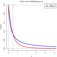
Figure 1: The variances of $\Phi\left(\rho\Phi^{-1}\left(\cdot\right)\right)$ and $\mathrm{Beta}\left(\rho,\rho\right)$ versus $\rho$.

Figure 1 shows $\mathrm{Var}\left(Z_{\rho,0}\right)$, $\mathrm{Var}\left(\mathrm{Beta}\left(\rho,\rho\right)\right)=\nicefrac{{1}}{{4\left(2\rho+1\right)}}$ versus $\rho$. Note that

$$\mathrm{Var}\left(Z_{\rho,0}\right)\gtreqqless\mathrm{Var}\left(\mathrm{Beta}\left(\rho,\rho\right)\right)\textrm{ when }\rho\lesseqqgtr 1$$ (12)

and that both converge monotonically to $\nicefrac{{1}}{{4}}$ when $\rho\rightarrow 0^{+}$ and to 0 when $\rho\rightarrow\infty$. Section 2.2.3 shows that standardized $Z_{\rho,\delta}$ becomes normal as $\rho\rightarrow\infty$.

2.1.2 The Case $\delta\in\mathbb{R}$

We return to the general setting—the setting in which $\rho\in\left(0,\infty\right)$ and $\delta\in\mathbb{R}$—deriving expressions for the mean, mode, and variance of $\Phi\left(\delta+\rho\Phi^{-1}\left(\cdot\right)\right)$. As above, we start with a statement about symmetry.

Theorem 2.5.

We have $f_{\rho,-\delta}\left(y\right)=f_{\rho,\delta}\left(1-y\right)$ for $f_{\rho,\delta}$ in (7) and $0<y<1$.

Proof.

Appendix B proves Theorem 2.5. ∎

Corollary 2.6.

$\mathbb{E}Z_{\rho,-\delta}=1-\mathbb{E}Z_{\rho,\delta}$ and $\mathrm{Var}\left(Z_{\rho,\delta}\right)=\mathrm{Var}\left(Z_{\rho,-\delta}\right)$ for $Z_{\rho,\delta}\sim\Phi\left(\delta+\rho\Phi^{-1}\left(\cdot\right)\right)$.

Proof.

Appendix B proves Corollary 2.6. ∎

Remark 2.7.

Note that:

1. Theorem 2.5 and Corollary 2.6 generalize Lemma 2.1 and Corollary 2.2.

2. Corollary 2.6 generalizes to $\mathbb{E}Z_{\rho,-\delta}^{k}=\sum_{j=0}^{k}\binom{k}{j}\left(-1\right)^{j}\mathbb{E}Z_{\rho,\delta}^{j}$, for $k\geq 1$.

3. For $b_{\alpha,\beta}$ the density of $X_{\alpha,\beta}\sim\mathrm{Beta}\left(\alpha,\beta\right)$, we have $b_{\alpha,\beta}\left(y\right)=b_{\beta,\alpha}\left(1-y\right)$, so that

   $$\mathbb{E}X_{\beta,\alpha}^{k}=\sum_{j=0}^{k}\binom{k}{j}\left(-1\right)^{j}\mathbb{E}X_{\alpha,\beta}^{j}$$ (13)

   for $k\geq 1$. Flipping the sign of $\delta$ is to $\Phi\left(\delta+\rho\Phi^{-1}\left(\cdot\right)\right)$ as swapping $\alpha$ and $\beta$ is to $\mathrm{Beta}\left(\alpha,\beta\right)$ (cf. Figure 2).

Theorem 2.8.

For $Z_{\rho,\delta}$ as above, $\mathbb{E}Z_{\rho,\delta}=\Pr\left(X_{1}\leq X_{0}\right)=\Phi\left(\nicefrac{{-\delta}}{{\sqrt{\rho^{2}+1}}}\right)$.

Proof.

Appendix B proves Theorem 2.8. ∎

Remark 2.9.

Theorem 2.8 generalizes Corollary 2.2 and comports with Corollary 2.6.

Proposition 2.10.

We have $0<\mathrm{Var}\left(Z_{\rho,\delta}\right)<\Phi\left(\nicefrac{{-\delta}}{{\sqrt{\rho^{2}+1}}}\right)\Phi\left(\nicefrac{{\delta}}{{\sqrt{\rho^{2}+1}}}\right)\leq\nicefrac{{1}}{{4}}$ for $\left(\rho,\delta\right)\in\left(0,\infty\right)\times\mathbb{R}$, so that $\lim_{\left|\delta\right|\rightarrow\infty}\mathrm{Var}\left(Z_{\rho,\delta}\right)=0$.

Proof.

Appendix B proves Proposition 2.10. ∎

We turn to the modes of $\Phi\left(\delta+\rho\Phi^{-1}\left(\cdot\right)\right)$, noting first that, if we let $b_{\alpha,\beta}\left(y\right)$ represent the $\mathrm{Beta}\left(\alpha,\beta\right)$ density (with $\alpha,\beta>0$), we have

$$\underset{0\leq y\leq 1}{\arg\max}\,b_{\alpha,\beta}\left(y\right)=\left\{\begin{array}[]{rl}\frac{\alpha-1}{\alpha+\beta-2}&\textrm{ if }\alpha,\beta>1\\ \left(0,1\right)&\textrm{ if }\alpha=\beta=1\\ \left\{0,1\right\}&\textrm{ if }\alpha,\beta<1\\ 0&\textrm{ if }\alpha\leq 1,\beta>1\\ 1&\textrm{ if }\alpha>1,\beta\leq 1\end{array}\right.$$ (14)

and

$$\max_{0\leq y\leq 1}b_{\alpha,\beta}\left(y\right)=\left\{\begin{array}[]{rl}\frac{\Gamma\left(\alpha+\beta\right)}{\Gamma\left(\alpha\right)\Gamma\left(\beta\right)}\frac{\left(\alpha-1\right)^{\alpha-1}\left(\beta-1\right)^{\beta-1}}{\left(\alpha+\beta-2\right)^{\alpha+\beta-2}}&\textrm{ if }\alpha,\beta>1\\ 1&\textrm{ if }\alpha=\beta=1\\ \infty&\textrm{ if }\alpha,\beta<1\\ \infty&\textrm{ if }\alpha<1,\beta>1\\ \infty&\textrm{ if }\alpha>1,\beta<1\\ \beta&\textrm{ if }\alpha=1,\beta>1\\ \alpha&\textrm{ if }\alpha>1,\beta=1\end{array}\right.$$ (15)

Note that $\max_{y}b_{\alpha,\beta}\left(y\right)$ breaks the $\left\{\alpha\leq 1,\beta>1\right\}$ and $\left\{\alpha>1,\beta\leq 1\right\}$ cases of $\arg\max_{y}b_{\alpha,\beta}\left(y\right)$ into $\left\{\alpha<1,\beta>1\right\}\cup\left\{\alpha=1,\beta>1\right\}$ and $\left\{\alpha>1,\beta<1\right\}\cup\left\{\alpha>1,\beta=1\right\}$. The modes and maxima of $\Phi\left(\delta+\rho\Phi^{-1}\left(\cdot\right)\right)$ follow a pattern similar to that of $\mathrm{Beta}\left(\alpha,\beta\right)$, but not in this particular regard.

Theorem 2.11.

With $f_{\rho,\delta}\left(y\right)$ as in (7),

$$\underset{0\leq y\leq 1}{\arg\max}\,f_{\rho,\delta}\left(y\right)=\left\{\begin{array}[]{rl}\Phi\left(-\frac{\rho\delta}{\rho^{2}-1}\right)&\textrm{ if }\rho>1\\ \left(0,1\right)&\textrm{ if }\rho=1,\delta=0\\ \left\{0,1\right\}&\textrm{ if }\rho<1\\ 0&\textrm{ if }\rho=1,\delta>0\\ 1&\textrm{ if }\rho=1,\delta<0\end{array}\right.$$ (16)

and

$$\max_{0\leq y\leq 1}f_{\rho,\delta}\left(y\right)=\left\{\begin{array}[]{rl}\rho\exp\left(\frac{\delta^{2}}{2\left(\rho^{2}-1\right)}\right)&\textrm{ if }\rho>1\\ 1&\textrm{ if }\rho=1,\delta=0\\ \infty&\textrm{ if }\rho<1\\ \infty&\textrm{ if }\rho=1,\delta>0\\ \infty&\textrm{ if }\rho=1,\delta<0\end{array}\right.$$ (17)

Proof.

Appendix B proves Theorem 2.11. ∎

Remark 2.12.

Theorem 2.11 generalizes Lemma 2.3.

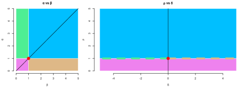
Figure 2: The mapping of $\left(\alpha,\beta\right)\in\left(0,\infty\right)^{2}$ to $\left(\rho,\delta\right)\in\left(0,\infty\right)\times\mathbb{R}$ suggested by the $\arg\max$ function, cf. (14) and (16). Colors correspond to modes: red=$\left(0,1\right)$, fuchsia=$\left\{0,1\right\}$, tan=0, green=1, blue=some function of the input parameters.

The beta and $\Phi\left(\delta+\rho\Phi^{-1}\left(\cdot\right)\right)$ distributions have similar modes ((14), (16)) and maxima ((15), (17)). Figure 2 shows the mapping between parameter spaces induced by the $\arg\max$ function (cf. (14) and (16)). In either plot we use blue to highlight regions of the parameter space where the mode depends on the input parameters (through $\nicefrac{{\left(\alpha-1\right)}}{{\left(\alpha+\beta-2\right)}}$ or $\Phi\left(\nicefrac{{-\rho\delta}}{{\left(\rho^{2}-1\right)}}\right)$). Non-blue colors highlight pairs of regions with identical modes ($\left(0,1\right),\left\{0,1\right\},0,\textrm{ or }1$). Section 2.3 explores several mappings from $\left(\rho,\delta\right)\in\left(0,\infty\right)\times\mathbb{R}$ to $\left(\alpha,\beta\right)\in\left(0,\infty\right)^{2}$.

We now turn to the difficult task of deriving an expression for the variance of $\Phi\left(\delta+\rho\Phi^{-1}\left(\cdot\right)\right)$.

Theorem 2.13.

Let

$$B_{\rho,\delta}\left(\theta\right) \coloneqq\frac{\sqrt{6}\delta\sin\left(\theta+\nicefrac{{\pi}}{{4}}\right)}{\rho^{2}+2}$$ (18)

$$A_{\rho}\left(\theta\right) \coloneqq\frac{\rho^{2}\left(\sin\left(2\theta\right)+2\right)+2\cos^{2}\left(\theta+\nicefrac{{\pi}}{{4}}\right)}{2\rho^{2}\left(\rho^{2}+2\right)}$$ (19)

$$G_{\rho,\delta}\left(\theta\right) \coloneqq\frac{\sqrt{3}e^{-\frac{\delta^{2}}{\rho^{2}+2}}}{2\pi\rho\sqrt{\rho^{2}+2}}\frac{B_{\rho,\delta}\left(\theta\right)}{\left[2A_{\rho}\left(\theta\right)\right]^{\nicefrac{{3}}{{2}}}}\frac{\Phi\left(\frac{B_{\rho,\delta}\left(\theta\right)}{\sqrt{2A_{\rho}\left(\theta\right)}}\right)}{\phi\left(\frac{B_{\rho,\delta}\left(\theta\right)}{\sqrt{2A_{\rho}\left(\theta\right)}}\right)}$$ (20)

If $Z_{\rho,\delta}\sim\Phi\left(\delta+\rho\Phi^{-1}\left(\cdot\right)\right)$, then

$$\mathrm{Var}\left(Z_{\rho,\delta}\right) =\Pr\left(X_{1}\leq X_{0},X_{2}\leq X_{0}\right)-\Pr\left(X_{1}\leq X_{0}\right)\Pr\left(X_{2}\leq X_{0}\right)$$ (21)

$$=\int_{\nicefrac{{11\pi}}{{12}}}^{\nicefrac{{19\pi}}{{12}}}G_{\rho,\delta}\left(\theta\right)d\theta+\frac{\cos^{-1}\left(\nicefrac{{-1}}{{\left(\rho^{2}+1\right)}}\right)}{2\pi\exp\left(\nicefrac{{\delta^{2}}}{{\left(\rho^{2}+2\right)}}\right)}-\Phi\left(\nicefrac{{-\delta}}{{\sqrt{\rho^{2}+1}}}\right)^{2}$$ (22)

Proof.

Appendix B proves Theorem 2.13. ∎

Remark 2.14.

Note that:

1. With $G_{\rho,0}\left(\theta\right)=B_{\rho,0}\left(\theta\right)=0$, Theorem 2.13 generalizes Lemma 2.4.

2. $G_{\rho,\delta}$ has even symmetry in $\theta$ about $\nicefrac{{5\pi}}{{4}}$ (see Lemma B.1); i.e., $\mathrm{Var}\left(Z_{\rho,\delta}\right)$

   $$=2\int_{\nicefrac{{11\pi}}{{12}}}^{\nicefrac{{5\pi}}{{4}}}G_{\rho,\delta}\left(\theta\right)d\theta+\frac{\cos^{-1}\left(\nicefrac{{-1}}{{\left(\rho^{2}+1\right)}}\right)}{2\pi\exp\left(\nicefrac{{\delta^{2}}}{{\left(\rho^{2}+2\right)}}\right)}-\Phi\left(\nicefrac{{-\delta}}{{\sqrt{\rho^{2}+1}}}\right)^{2}$$ (23)

   $$=2\int_{\nicefrac{{5\pi}}{{4}}}^{\nicefrac{{19\pi}}{{12}}}G_{\rho,\delta}\left(\theta\right)d\theta+\frac{\cos^{-1}\left(\nicefrac{{-1}}{{\left(\rho^{2}+1\right)}}\right)}{2\pi\exp\left(\nicefrac{{\delta^{2}}}{{\left(\rho^{2}+2\right)}}\right)}-\Phi\left(\nicefrac{{-\delta}}{{\sqrt{\rho^{2}+1}}}\right)^{2}$$ (24)

3. For any $k\geq 1$, $\mathbb{E}Z_{\rho,\delta}^{k}=\Pr\left(X_{0}\geq\max\left\{X_{1},X_{2},\ldots,X_{k}\right\}\right)$ (see the proof of Proposition 4.9 in Appendix H).

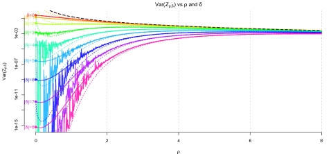
Figure 3: The variance of $\Phi\left(\delta+\rho\Phi^{-1}\left(\cdot\right)\right)$ versus $\rho$ and $\delta$. Smooth, solid curves (indexed by $\left|\delta\right|$; Corollary 2.6) give $\mathrm{Var}\left(Z_{\rho,\delta}\right)$ from $\textrm{\eqref{eq:varIntApprox}}\approx\textrm{\eqref{eq:varZrhodelta}}$. Jagged curves use simulations to approximate $\mathrm{Var}\left(Z_{\rho,\delta}\right)$ (see (26)). Note that $\mathrm{Var}\left(Z_{\rho,\delta}\right)\sim\nicefrac{{1}}{{2\pi\rho^{2}}}$ as $\rho\rightarrow\infty$ (dashed curve; see (29)) and that $\mathrm{Var}\left(Z_{\rho,\delta}\right)\sim\nicefrac{{\phi\left(\nicefrac{{\delta}}{{\sqrt{\rho^{2}+1}}}\right)^{2}}}{{\rho^{2}}}$ as $\rho,\left|\delta\right|\rightarrow\infty$ and $\nicefrac{{\delta}}{{\rho}}$ remains fixed (dotted curve; see (31)). Small circles above $\rho=0$ illustrate Proposition 2.17. The logarithmic scale of the $y$-axis exaggerates the noisiness of smaller estimates of $\mathrm{Var}\left(Z_{\rho,\delta}\right)$, i.e., those from (26) and (31).

Figure 3 shows $\mathrm{Var}\left(Z_{\rho,\left|\delta\right|}\right)=\mathrm{Var}\left(Z_{\rho,\pm\delta}\right)$ versus $0<\rho\leq 8$ and $0\leq\left|\delta\right|\leq 8$ (Corollary 2.6). Note that:

1. We approximate $\mathrm{Var}\left(Z_{\rho,\delta}\right)$ in (22) using

   $$\epsilon\sum_{k=0}^{\left\lfloor\nicefrac{{2\pi}}{{3\epsilon}}\right\rfloor}G_{\rho,\delta}\left(\frac{11\pi}{12}+k\epsilon\right)+\frac{\cos^{-1}\left(\nicefrac{{-1}}{{\left(\rho^{2}+1\right)}}\right)}{2\pi\exp\left(\nicefrac{{\delta^{2}}}{{\left(\rho^{2}+2\right)}}\right)}-\Phi\left(\nicefrac{{-\delta}}{{\sqrt{\rho^{2}+1}}}\right)^{2}$$ (25)

   with $\epsilon\coloneqq 10^{-4}$, splitting $\left[\nicefrac{{11\pi}}{{12}},\nicefrac{{19\pi}}{{12}}\right)$ into $\left\lceil\nicefrac{{2\pi}}{{3\epsilon}}\right\rceil>$ 20,000 equal-width bins (the final bin is slightly smaller than the others).

2. Figure 3 shows simulation-based estimates of $\mathrm{Var}\left(Z_{\rho,\delta}\right)$, which we obtain as follows. Fixing $\left(\rho,\delta\right)\in\left(0,8\right]\times\left[0,8\right]$ and letting $m\coloneqq 10^{4}$, we sample $\left\{X_{0,j}\right\}_{1}^{m}$ from $\mathcal{N}\left(0,1\right)$, let $Z_{j}\coloneqq\Phi\left(\nicefrac{{\left(X_{0,j}-\delta\right)}}{{\rho}}\right)$ ($1\leq j\leq m$), and compute

   $$\widehat{\mathrm{Var}}\left(Z_{\rho,\delta}\right)\coloneqq\frac{1}{m-1}\sum_{j=1}^{m}\left(Z_{j}-\frac{1}{m}\sum_{j^{\prime}=1}^{m}Z_{j^{\prime}}\right)^{2}$$ (26)

   Estimates $\widehat{\mathrm{Var}}\left(Z_{\rho,\delta}\right)$ are overly small for $\rho$ small and $\left|\delta\right|$ large. Figure 3’s logarithmic vertical scale makes smaller estimates look excessively noisy. Estimate (26) approaches $\textrm{\eqref{eq:varIntApprox}}\approx\textrm{\eqref{eq:varZrhodelta}}$ for larger $\rho$ and smaller $\left|\delta\right|$.

3. Figure 3 suggests that $\mathrm{Var}\left(Z_{\rho,\delta}\right)$ approaches 0 monotonically as $\left|\delta\right|\rightarrow\infty$. See Propositions 2.10 and 2.15.

4. Figure 3 suggests that $2\pi\rho^{2}\mathrm{Var}\left(Z_{\rho,\delta}\right)$ approaches 1 as $\rho\rightarrow\infty$. Proposition 2.18 shows this analytically.

5. Figure 3 suggests that $\left.\rho^{2}\mathrm{Var}\left(Z_{\rho,\delta}\right)\right/\phi\left(\nicefrac{{\delta}}{{\sqrt{\rho^{2}+1}}}\right)^{2}$ approaches 1 as $\rho,\left|\delta\right|\rightarrow\infty$ and $\nicefrac{{\delta}}{{\rho}}$ remains fixed. Proposition 2.20 shows this analytically.

Finally, as suggested by Figure 3, we note that:

Proposition 2.15.

If $Z_{\rho,\delta}\sim\Phi\left(\delta+\rho\Phi^{-1}\left(\cdot\right)\right)$ and $\left|\delta_{1}\right|<\left|\delta_{2}\right|$, then $\mathrm{Var}\left(Z_{\rho,\delta_{1}}\right)>\mathrm{Var}\left(Z_{\rho,\delta_{2}}\right)$.

Proof.

Appendix B proves Proposition 2.15. ∎

2.2 The Asymptotics of $Z_{\rho,\delta}$

We now derive asymptotic distributions for $Z_{\rho,\delta}\sim\Phi\left(\delta+\rho\Phi^{-1}\left(\cdot\right)\right)$ as $\left|\delta\right|\rightarrow\infty$ (§2.2.1); as $\rho\rightarrow 0^{+}$ (§2.2.2); as $\rho\rightarrow\infty$ (§2.2.3); and as $\rho,\left|\delta\right|\rightarrow\infty$ while keeping $\nicefrac{{\delta}}{{\rho}}$ fixed (§2.2.4).

2.2.1 When $\left|\delta\right|\rightarrow\infty$

In this setting we have $\mu_{0}\gg\mu$ or $\mu_{0}\ll\mu$. Proposition 2.10 then implies that:

Proposition 2.16.

For $Z_{\rho,\delta}$ as above, $Z_{\rho,\delta}\stackrel{{\scriptstyle[}}{{\infty}}]{\delta}{\longrightarrow}0$ and $Z_{\rho,\delta}\stackrel{{\scriptstyle[}}{{-}}\infty]{\delta}{\longrightarrow}1$ in probability.

Proof.

Appendix C proves Proposition 2.16. ∎

2.2.2 When $\rho\rightarrow 0^{+}$

The case with $\rho=0$, i.e., $\sigma_{0}^{2}\gg\sigma^{2}$, is not $\Phi\left(\delta+\rho\Phi^{-1}\left(\cdot\right)\right)$-distributed. Instead,

Proposition 2.17.

If $Z_{\rho,\delta}\sim\Phi\left(\delta+\rho\Phi^{-1}\left(\cdot\right)\right)$, $Z_{\rho,\delta}\implies\mathrm{Bernoulli}\left(\Phi\left(-\delta\right)\right)$, where $\implies$ indicates convergence in distribution as $\rho\rightarrow 0^{+}$.

Proof.

Appendix C proves Proposition 2.17. ∎

As we illustrate in Figures 1 and 3, Proposition 2.17 gives

$$\lim_{\rho\rightarrow 0^{+}}\mathrm{Var}\left(Z_{\rho,\delta}\right)=\Phi\left(-\delta\right)\Phi\left(\delta\right)>0$$ (27)

so that $Z_{\rho,\delta}$ is non-degenerate as $\rho\rightarrow 0^{+}$, in contrast to the situations in which $\left|\delta\right|\rightarrow\infty$ (Proposition 2.16); $\rho\rightarrow\infty$ (Corollary 2.19); and $\rho,\left|\delta\right|\rightarrow\infty$ while $\nicefrac{{\delta}}{{\rho}}=r$ remains fixed (Corollary 2.21). Letting $\rho\rightarrow 0^{+}$ and $\left|\delta\right|\rightarrow\infty$ (in either order) returns us to the degenerate case. Theorem 2.8 and Proposition 2.17 give $\lim_{\rho\rightarrow 0^{+}}\mathbb{E}Z_{\rho,\delta}=\Phi\left(-\delta\right)$.

2.2.3 When $\rho\rightarrow\infty$

If $\sigma_{0}^{2}\ll\sigma^{2}$, then $Z_{\rho,\delta}$ (properly standardized) approaches normality.

Proposition 2.18.

If $Z_{\rho,\delta}\sim\Phi\left(\delta+\rho\Phi^{-1}\left(\cdot\right)\right)$, then

$$\rho\left\{Z_{\rho,\delta}-\Phi\left(\nicefrac{{-\delta}}{{\sqrt{\rho^{2}+1}}}\right)\right\}\implies\mathcal{N}\left(0,\nicefrac{{1}}{{2\pi}}\right)$$ (28)

where $\implies$ indicates convergence in distribution as $\rho\rightarrow\infty$.

Proof.

Appendix C proves Proposition 2.18. ∎

From Proposition 2.18 we have

$$Z_{\rho,\delta}\stackrel{{\scriptstyle.}}{{\sim}}\mathcal{N}\left(\Phi\left(-\frac{\delta}{\sqrt{\rho^{2}+1}}\right),\frac{1}{2\pi\rho^{2}}\right)$$ (29)

when $\rho$ is large. Note that $\mathrm{Var}\left(Z_{\rho,\delta}\right)\approx\nicefrac{{1}}{{2\pi\rho^{2}}}$ when $\rho>4\left|\delta\right|$ (Figure 3), so that:

Corollary 2.19.

With $Z_{\rho,\delta}$ as above, $Z_{\rho,\delta}\longrightarrow\nicefrac{{1}}{{2}}$ in probability as $\rho\rightarrow\infty$.

Proof.

Appendix C proves Corollary 2.19. ∎

As the $X_{i}$ become more and more variable relative to $X_{0}$, $\Phi\left(\nicefrac{{\left(X_{0}-\mu\right)}}{{\sigma}}\right)$ places more and more of its mass near $\nicefrac{{1}}{{2}}$. As we go about characterizing $\mathscr{L}\left(R_{0}\right)$ (the rank of the odd normal out), $\Phi\left(\delta+\rho\Phi^{-1}\left(\cdot\right)\right)$ plays the role of the prior from the standard beta-binomial setting (cf. (2)). Increasing $\sigma^{2}$ relative to $\sigma_{0}^{2}$ (i.e., increasing $\rho$) concentrates the prior around $\nicefrac{{1}}{{2}}$, thereby pushing the finitely-variable $X_{0}$ to bisect the infinitely-variable $X_{i}$, $1\leq i\leq n$, as expected.

2.2.4 When $\rho,\left|\delta\right|\rightarrow\infty$ While $\nicefrac{{\delta}}{{\rho}}$ Remains Fixed

In this setting, where $\mu_{0}\gg\mu$ or $\mu_{0}\ll\mu$ and $\sigma_{0}^{2}\ll\sigma^{2}$ in such a way that $\frac{\delta}{\rho}=\frac{\mu-\mu_{0}}{\sigma}$ remains fixed, $Z_{\rho,\delta}$ (properly standardized) approaches normality.

Proposition 2.20.

Fix $r\in\mathbb{R}$. Let $\delta=r\rho$. If $Z_{\rho,\delta}\sim\Phi\left(\delta+\rho\Phi^{-1}\left(\cdot\right)\right)$, then

$$\rho\left\{Z_{\rho,\delta}-\Phi\left(\nicefrac{{-\delta}}{{\sqrt{\rho^{2}+1}}}\right)\right\}\implies\mathcal{N}\left(0,\phi\left(r\right)^{2}\right)$$ (30)

where $\implies$ gives convergence in distribution as $\rho,\left|\delta\right|\rightarrow\infty$ and $\nicefrac{{\delta}}{{\rho}}=r$ remains fixed.

Proof.

Appendix C proves Proposition 2.20. ∎

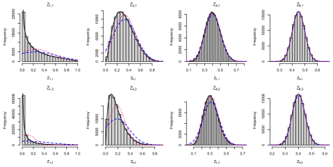
Figure 4: Simulated $Z_{\rho,\delta}^{\left(j\right)}\stackrel{{\scriptstyle\mathrm{iid}}}{{\sim}}\Phi\left(\delta+\rho\Phi^{-1}\left(\cdot\right)\right)$ for $\left(\rho,\delta\right)\in\left\{1,2,4,8\right\}\times\left\{1,2\right\}$ and $1\leq j\leq 10^{5}$. Blue, pink, and black curves give normal approximations (29), (31) and true density (7). Approximation (31) outperforms approximation (29). Approximations (29) and (31) approach each other as $\nicefrac{{\rho}}{{\left|\delta\right|}}$ becomes large.

According to Proposition 2.20, for large $\min\left(\rho,\left|\delta\right|\right)$,

$$Z_{\rho,\delta}\stackrel{{\scriptstyle.}}{{\sim}}\mathcal{N}\left(\Phi\left(-\frac{\delta}{\sqrt{\rho^{2}+1}}\right),\frac{\phi\left(\nicefrac{{\delta}}{{\sqrt{\rho^{2}+1}}}\right)^{2}}{\rho^{2}}\right)$$ (31)

The variance in (31), with its dependence on $\delta$, improves on that in (29) (Figure 3); i.e., the normal distribution in (31)—as compared with that in (29)—better approximates $\mathscr{L}\left(Z_{\rho,\delta}\right)$ (Figure 4). Approximations (29) and (31) approach each other as $\nicefrac{{\rho}}{{\left|\delta\right|}}$ becomes large. The variance in (31) further implies that:

Corollary 2.21.

With $Z_{\rho,\delta}$ as above, $Z_{\rho,\delta}\longrightarrow\Phi\left(-r\right)$ in probability as $\rho,\left|\delta\right|\rightarrow\infty$ and $\nicefrac{{\delta}}{{\rho}}=r$ remains fixed.

Proof.

Appendix C proves Corollary 2.21. ∎

Increasing $\sigma^{2}$ relative to $\sigma_{0}^{2}$ and increasing $\left|\mu-\mu_{0}\right|$ in such a way that $\frac{\delta}{\rho}=\frac{\mu-\mu_{0}}{\sigma}\eqqcolon r$ remains fixed concentrates $\mathscr{L}\left(Z_{\rho,\delta}\right)$ about $\Phi\left(-r\right)$.

The normality of $Z_{\rho,\delta}$ as $\rho$ (and optionally $\left|\delta\right|$) becomes large provides yet another point of similarity between $\mathrm{Beta}\left(\alpha,\beta\right)$ and $\Phi\left(\delta+\rho\Phi^{-1}\left(\cdot\right)\right)$ (cf. Remark 2.7 and Figure 2).

2.3 Finding the Proximal Beta

Sections 2.1 and 2.2 show numerous points of similarity between $\mathrm{Beta}\left(\alpha,\beta\right)$ and $\Phi\left(\delta+\rho\Phi^{-1}\left(\cdot\right)\right)$:

1. $\mathrm{Beta}\left(\alpha,\alpha\right)$ and $\Phi\left(\rho\Phi^{-1}\left(\cdot\right)\right)$ are symmetric about $\nicefrac{{1}}{{2}}$, i.e., $b_{\alpha,\alpha}\left(1-y\right)=b_{\alpha,\alpha}\left(y\right)$ and $f_{\rho,0}\left(1-y\right)=f_{\rho,0}\left(y\right)$ (Lemma 2.1 and Corollary 2.2).

2. Swapping $\alpha$ and $\beta$ is to $\mathrm{Beta}\left(\alpha,\beta\right)$ as negating $\delta$ is to $\Phi\left(\delta+\rho\Phi^{-1}\left(\cdot\right)\right)$, viz., $b_{\alpha,\beta}\left(y\right)=b_{\beta,\alpha}\left(1-y\right)$ and $f_{\rho,\delta}\left(y\right)=f_{\rho,-\delta}\left(1-y\right)$ (Theorem 2.5, Corollary 2.6, and Remark 2.7).

3. Both have parameter configurations that yield $\mathrm{Unif}\left(0,1\right)$, i.e., $\mathscr{L}\left(X_{1,1}\right)=\mathscr{L}\left(Z_{1,0}\right)=\mathrm{Unif}\left(0,1\right)$, for $X_{\alpha,\beta}\sim\mathrm{Beta}\left(\alpha,\beta\right)$ and $Z_{\rho,\delta}\sim\Phi\left(\delta+\rho\Phi^{-1}\left(\cdot\right)\right)$ (Lemma 2.3, Theorem 2.11, and Figure 2).

4. $\mathrm{Beta}\left(\alpha,\beta\right)$ and $\Phi\left(\delta+\rho\Phi^{-1}\left(\cdot\right)\right)$ have the same modes if we exclude one of each that depend on input parameters (Theorem 2.11 and Figure 2).

5. Both converge to normality as parameters grow (Propositions 2.18 and 2.20 and Lemma 2.26). Either setting provides situations in which parameters grow while keeping certain relationships between themselves fixed.

These similarities, taken in aggregate, suggest using $\mathrm{Beta}\left(\alpha,\beta\right)$ to approximate $\Phi\left(\delta+\rho\Phi^{-1}\left(\cdot\right)\right)$ in order to characterize $X_{0}$’s rank (cf. (2)). This in turn leads us to consider mappings from the $\Phi\left(\delta+\rho\Phi^{-1}\left(\cdot\right)\right)$ parameter space $\left(0,\infty\right)\times\mathbb{R}$ to the $\mathrm{Beta}\left(\alpha,\beta\right)$ parameter space $\left(0,\infty\right)^{2}$. With

$$W_{2}\left(X,Y\right)\coloneqq\sqrt{\int_{0}^{1}\left\{F_{X}^{-1}\left(z\right)-F_{Y}^{-1}\left(z\right)\right\}^{2}dz}$$ (32)

the 2-Wasserstein distance between $X\sim F_{X}$ and $Y\sim F_{Y}$, one might find

$$\left[\alpha\left(\rho,\delta\right),\beta\left(\rho,\delta\right)\right]\coloneqq\underset{\left(\alpha,\beta\right)\in\left(0,\infty\right)^{2}}{\arg\min}W_{2}\left(X_{\alpha,\beta},Z_{\rho,\delta}\right)$$ (33)

for $X_{\alpha,\beta}\sim\mathrm{Beta}\left(\alpha,\beta\right)$ and $Z_{\rho,\delta}\sim\Phi\left(\delta+\rho\Phi^{-1}\left(\cdot\right)\right)$ such that $\alpha\left(\rho,\delta\right)$ and $\beta\left(\rho,\delta\right)$ are easy to compute. We do not solve (33). Instead, we propose three mappings,

$$\alpha_{j} :\left(0,\infty\right)\times\mathbb{R}\longrightarrow\left(0,\infty\right)$$ (34)

$$\beta_{j} :\left(0,\infty\right)\times\mathbb{R}\longrightarrow\left(0,\infty\right)$$ (35)

for $1\leq j\leq 3$, and pick the best one. The third mapping (based on matching means and variances) has the following, advantageous properties:

1. It is easy to compute. (The first mapping—not relying on $\mathrm{Var}\left(Z_{\rho,\delta}\right)$—is easier to compute; see (25). The computation of the second mapping—as implemented here—is numerically unstable and often fails.)

2. The set $\left\{\left(\rho,\delta\right)\in\left(0,\infty\right)\times\mathbb{R}:W_{2}\left(Z_{\rho,\delta},X_{\alpha_{1},\beta_{1}}\right)<W_{2}\left(Z_{\rho,\delta},X_{\alpha_{3},\beta_{3}}\right)\right\}$ is apparently bounded (Figures 5 and 6) although we do not prove this.

3. $W_{2}\left(Z_{\rho,\delta},X_{\alpha_{3},\beta_{3}}\right)\rightarrow 0$ as $\left|\delta\right|\rightarrow\infty$; as $\rho\rightarrow 0^{+}$; as $\rho\rightarrow\infty$; and as $\rho,\left|\delta\right|\rightarrow\infty$ while $\nicefrac{{\delta}}{{\rho}}$ remains fixed (see section 2.4).

4. It produces an approximation $R^{\prime}_{0}$ for which $\mathbb{E}R^{\prime}_{0}=\mathbb{E}R_{0}$ and $\mathrm{Var}\left(R^{\prime}_{0}\right)=\mathrm{Var}\left(R_{0}\right)$ (see Theorem 3.4, Proposition 3.7, and Remark 3.8).

Sections 2.3.1–2.3.3 describe these mappings, of which we use the third. Section 2.4 then shows that $W_{2}\left(Z_{\rho,\delta},X_{\alpha_{3},\beta_{3}}\right)\rightarrow 0$ as $\left|\delta\right|\rightarrow\infty$; as $\rho\rightarrow 0^{+}$; as $\rho\rightarrow\infty$; and as $\rho,\left|\delta\right|\rightarrow\infty$ while $\nicefrac{{\delta}}{{\rho}}$ remains fixed.

2.3.1 Matching Means When $\boldsymbol{\rho}\approx\mathbf{1}$

When $\rho\approx 1$, we let $\mathbb{E}X_{\alpha,\beta}=\mathbb{E}Z_{\rho,\delta}$ (Theorem 2.8) and $\alpha\beta=\rho$ (Figure 2). This leads to

$$\alpha_{1}\left(\rho,\delta\right) \coloneqq\sqrt{\rho\left.\Phi\left(\nicefrac{{-\delta}}{{\sqrt{\rho^{2}+1}}}\right)\right/\Phi\left(\nicefrac{{\delta}}{{\sqrt{\rho^{2}+1}}}\right)}$$ (36)

$$\beta_{1}\left(\rho,\delta\right) \coloneqq\sqrt{\rho\left.\Phi\left(\nicefrac{{\delta}}{{\sqrt{\rho^{2}+1}}}\right)\right/\Phi\left(\nicefrac{{-\delta}}{{\sqrt{\rho^{2}+1}}}\right)}$$ (37)

With $W_{2}$ the 2-Wasserstein distance in (32), Figure 5 shows

$$W_{2}\left(X_{\alpha_{1}\left(\rho,\delta\right),\beta_{1}\left(\rho,\delta\right)},Z_{\rho,\delta}\right)$$ (38)

for $X_{\alpha,\beta}\sim\mathrm{Beta}\left(\alpha,\beta\right)$, $Z_{\rho,\delta}\sim\Phi\left(\delta+\rho\Phi^{-1}\left(\cdot\right)\right)$, $\alpha_{1}$ and $\beta_{1}$ from (36) and (37), and $\left(\rho,\delta\right)\in\left(0,\nicefrac{{15}}{{2}}\right]\times\left[\nicefrac{{-15}}{{2}},\nicefrac{{15}}{{2}}\right]$. From Figure 5 we see that $\mathrm{Beta}\left(\alpha_{1},\beta_{1}\right)\approx\Phi\left(\delta+\rho\Phi^{-1}\left(\cdot\right)\right)$ when $\rho\approx 1$. This region grows with $\left|\delta\right|$. That said, $\mathscr{L}\left(X_{\alpha_{1},\beta_{1}}\right)$ and $\mathscr{L}\left(Z_{\rho,\delta}\right)$ are often at a far remove, e.g., when $\left(\rho,\delta\right)\in\left\{\left(\nicefrac{{1}}{{10}},0\right),\left(7,0\right)\right\}$.

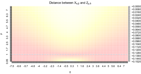
Figure 5: The Wasserstein distant between $X_{\alpha_{1}\left(\rho,\delta\right),\beta_{1}\left(\rho,\delta\right)}$ and $Z_{\rho,\delta}$ vs $\rho$ and $\delta$. The dashed line is $\rho=1$. See (36)–(38). The key is on the right. Figures 5–6 use different color scales. Here, $\mathrm{red}=\left[0,0.002\right)$, and $\mathrm{white}=\left[0.150,0.152\right)$. The median distance in Figure 5 is ninety times larger than that in Figure 6.

2.3.2 Matching Modes and Maxima

For $\rho>1$, $f_{\rho,\delta}\left(y\right)$ grows smaller as $\left|y-\Phi\left(\nicefrac{{-\rho\delta}}{{\left(\rho^{2}-1\right)}}\right)\right|$ grows larger (Theorem 2.11). As $\rho$ grows large, $Z_{\rho,\delta}$ approaches normality (Propositions 2.18, 2.20). Taking these things into account and assuming $\rho>1$, we define $\alpha_{2}$ and $\beta_{2}$ by

$$\underset{0\leq y\leq 1}{\arg\max}\,b_{\alpha_{2},\beta_{2}}\left(y\right) =\underset{0\leq y\leq 1}{\arg\max}\,f_{\rho,\delta}\left(y\right)$$ (39)

$$\max_{0\leq y\leq 1}b_{\alpha_{2},\beta_{2}}\left(y\right) =\max_{0\leq y\leq 1}f_{\rho,\delta}\left(y\right)$$ (40)

Given $\left(\rho,\delta\right)\in\left(1,\infty\right)\times\mathbb{R}$, we solve (39) and (40) for $\left(\alpha_{2},\beta_{2}\right)\in\left(1,\infty\right)^{2}$ as follows. First, (39) provides

$$\alpha_{2}=\frac{\Phi\left(\nicefrac{{-\rho\delta}}{{\left(\rho^{2}-1\right)}}\right)}{\Phi\left(\nicefrac{{\rho\delta}}{{\left(\rho^{2}-1\right)}}\right)}\left(\beta_{2}-1\right)+1$$ (41)

If we plug (41) into (40), uniroot and (40) give $\beta_{2}$ (R Core Team (2022)); $\beta_{2}$ and (41) give $\alpha_{2}$. The uniroot step often fails; the computation is numerically unstable. The mean-variance mapping below not only sidesteps these numerical issues, but more directly matches up distributional centers and spreads.

2.3.3 Matching Means and Variances

While $Z_{\rho,\delta}$ approaches normality as $\rho\rightarrow\infty$ (Proposition 2.18) or as $\rho,\left|\delta\right|\rightarrow\infty$ with $\nicefrac{{\delta}}{{\rho}}$ fixed (Proposition 2.20), we here let $\mathbb{E}X_{\alpha,\beta}=\mathbb{E}Z_{\rho,\delta}$ (Theorem 2.8) and $\mathrm{Var}\left(X_{\alpha,\beta}\right)=\mathrm{Var}\left(Z_{\rho,\delta}\right)$ (Theorem 2.13). This leads to

$$\alpha_{3}\left(\rho,\delta\right) \coloneqq\frac{\Phi\left(\nicefrac{{-\delta}}{{\sqrt{\rho^{2}+1}}}\right)}{\mathrm{Var}\left(Z_{\rho,\delta}\right)}\left[\Phi\left(\nicefrac{{-\delta}}{{\sqrt{\rho^{2}+1}}}\right)\Phi\left(\nicefrac{{\delta}}{{\sqrt{\rho^{2}+1}}}\right)-\mathrm{Var}\left(Z_{\rho,\delta}\right)\right]$$ (42)

$$\beta_{3}\left(\rho,\delta\right) \coloneqq\frac{\Phi\left(\nicefrac{{\delta}}{{\sqrt{\rho^{2}+1}}}\right)}{\mathrm{Var}\left(Z_{\rho,\delta}\right)}\left[\Phi\left(\nicefrac{{-\delta}}{{\sqrt{\rho^{2}+1}}}\right)\Phi\left(\nicefrac{{\delta}}{{\sqrt{\rho^{2}+1}}}\right)-\mathrm{Var}\left(Z_{\rho,\delta}\right)\right]$$ (43)

Note that:

1. In what follows we use $\textrm{\eqref{eq:varIntApprox}}\approx\textrm{\eqref{eq:varZrhodelta}}$ to compute $\mathrm{Var}\left(Z_{\rho,\delta}\right)$. An easier-to-compute, less precise option is $\mathrm{Var}\left(Z_{\rho,\delta}\right)\sim\rho^{-2}\phi\left(\nicefrac{{\delta}}{{\sqrt{\rho^{2}+1}}}\right)$ (see (31) and Figure 3). This option grows more accurate as $\rho$ and $\left|\delta\right|$ increase.

2. The bracketed term in (42)–(43) is positive (Proposition 2.10), which gives $\alpha_{3},\beta_{3}>0$. This approach (unlike the one in section 2.3.2) works for any $\left(\rho,\delta\right)\in\left(0,\infty\right)\times\mathbb{R}$.

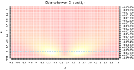
Figure 6: The Wasserstein distant between $X_{\alpha_{3}\left(\rho,\delta\right),\beta_{3}\left(\rho,\delta\right)}$ and $Z_{\rho,\delta}$ vs $\rho$ and $\delta$. The dashed line is $\rho=1$. See (42)–(44). The key is on the right. Figures 5–6 use different color scales. Here, $\mathrm{red}=\left[0,0.0001\right)$, and $\mathrm{white}=\left[0.0077,0.0078\right)$. The median distance in Figure 6 is ninety times smaller than that in Figure 5.

With $W_{2}$ the 2-Wasserstein distance in (32), Figure 6 shows

$$W_{2}\left(X_{\alpha_{3}\left(\rho,\delta\right),\beta_{3}\left(\rho,\delta\right)},Z_{\rho,\delta}\right)$$ (44)

for $X_{\alpha,\beta}\sim\mathrm{Beta}\left(\alpha,\beta\right)$, $Z_{\rho,\delta}\sim\Phi\left(\delta+\rho\Phi^{-1}\left(\cdot\right)\right)$, $\alpha_{3}$ and $\beta_{3}$ from (42) and (43), and $\left(\rho,\delta\right)\in\left(0,\nicefrac{{15}}{{2}}\right]\times\left[\nicefrac{{-15}}{{2}},\nicefrac{{15}}{{2}}\right]$. The color scale in Figure 6 does not match that in Figure 5; the median value in Figure 6 is ninety times smaller than that in Figure 5. $W_{2}\left(X_{\alpha_{3},\beta_{3}},Z_{\rho,\delta}\right)$ maxes out near $\left(\rho,\left|\delta\right|\right)=\left(0.85,1.9\right)$ at 0.0078. $W_{2}\left(X_{\alpha_{1},\beta_{1}},Z_{\rho,\delta}\right)$ maxes out near $\left(\rho,\delta\right)=\left(0.1,0\right)$ at 0.1511. Mapping (42)–(43) works well for almost all $\left(\rho,\delta\right)\in\left(0,\infty\right)\times\mathbb{R}$ (see section 2.4). In the sequel, when we need a mapping from $\left(\rho,\delta\right)$ to $\left(\alpha,\beta\right)$, we use the mean-variance mapping.

2.4 The Asymptotics of $X_{\alpha_{3}\left(\rho,\delta\right),\beta_{3}\left(\rho,\delta\right)}$

We show that $\mathscr{L}\left(Z_{\rho,\delta}\right)$ and $\mathscr{L}\left(X_{\alpha_{3}\left(\rho,\delta\right),\beta_{3}\left(\rho,\delta\right)}\right)$ become the same distribution, for $\alpha_{3}$ and $\beta_{3}$ in (42)–(43), as $\left|\delta\right|\rightarrow\infty$ (§2.4.1); as $\rho\rightarrow 0^{+}$ (§2.4.2); as $\rho\rightarrow\infty$ (§2.4.3); and as $\rho,\left|\delta\right|\rightarrow\infty$ while $\nicefrac{{\delta}}{{\rho}}$ remains fixed (§2.4.4). Specifically, we show that $W_{2}\left(X_{\alpha_{3}\left(\rho,\delta\right),\beta_{3}\left(\rho,\delta\right)},Z_{\rho,\delta}\right)\rightarrow 0$ in these settings, for $W_{2}$ the 2-Wasserstein distance in (32).

2.4.1 When $\left|\delta\right|\rightarrow\infty$

In this setting $\mu_{0}\gg\mu$ or $\mu_{0}\ll\mu$. We first note that:

Lemma 2.22.

For $X_{\alpha,\beta}\sim\mathrm{Beta}\left(\alpha,\beta\right)$, we have the following convergence in probability

$$X_{\alpha,\beta}\longrightarrow\left\{\begin{array}[]{rl}0&\textrm{ if }\beta\rightarrow\infty\textrm{ and }\alpha=o\left(\beta\right)\\ 1&\textrm{ if }\alpha\rightarrow\infty\textrm{ and }\beta=o\left(\alpha\right)\end{array}\right.$$ (45)

Proof.

Appendix D proves Lemma 2.22. ∎

Using Lemma 2.22 we then have:

Proposition 2.23.

For $X_{\alpha,\beta}\sim\mathrm{Beta}\left(\alpha,\beta\right)$ and $\alpha_{3}$ and $\beta_{3}$ in (42) and (43), we have the following convergence in probability

$$X_{\alpha_{3}\left(\rho,\delta\right),\beta_{3}\left(\rho,\delta\right)}\longrightarrow\left\{\begin{array}[]{rl}0&\textrm{ if }\delta\rightarrow\infty\\ 1&\textrm{ if }\delta\rightarrow-\infty\end{array}\right.$$ (46)

Then, for $Z_{\rho,\delta}\sim\Phi\left(\delta+\rho\Phi^{-1}\left(\cdot\right)\right)$ and $W_{2}$ the 2-Wasserstein metric in (32), we have $\lim_{\left|\delta\right|\rightarrow\infty}W_{2}\left(X_{\alpha_{3}\left(\rho,\delta\right),\beta_{3}\left(\rho,\delta\right)},Z_{\rho,\delta}\right)=0$.

Proof.

Appendix D proves Proposition 2.23. ∎

2.4.2 When $\rho\rightarrow 0^{+}$

We now turn to the setting in which $\sigma_{0}^{2}\gg\sigma^{2}$. We first note that:

Lemma 2.24.

For $X_{\alpha,\beta}\sim\mathrm{Beta}\left(\alpha,\beta\right)$ and $\lim_{\alpha,\beta\rightarrow 0^{+}}\nicefrac{{\alpha}}{{\left(\alpha+\beta\right)}}\eqqcolon\lambda\in\left(0,1\right)$,

$$X_{\alpha,\beta}\implies\mathrm{Bernoulli}\left(\lambda\right)$$ (47)

where $\implies$ indicates convergence in distribution as $\alpha,\beta\rightarrow 0^{+}$.

Proof.

Appendix D proves Lemma 2.24. ∎

Then, using Lemma 2.24, we have:

Proposition 2.25.

For $X_{\alpha,\beta}\sim\mathrm{Beta}\left(\alpha,\beta\right)$ and $\alpha_{3},\beta_{3}$ in (42), (43), we have

$$X_{\alpha_{3}\left(\rho,\delta\right),\beta_{3}\left(\rho,\delta\right)}\implies\mathrm{Bernoulli}\left(\Phi\left(-\delta\right)\right)$$ (48)

where $\implies$ gives convergence in distribution as $\rho\rightarrow 0^{+}$. This then implies that $\lim_{\rho\rightarrow 0^{+}}W_{2}\left(X_{\alpha_{3}\left(\rho,\delta\right),\beta_{3}\left(\rho,\delta\right)},Z_{\rho,\delta}\right)=0$ for $Z_{\rho,\delta}\sim\Phi\left(\delta+\rho\Phi^{-1}\left(\cdot\right)\right)$ and $W_{2}$ the 2-Wasserstein metric in (32).

Proof.

Appendix D proves Proposition 2.25. ∎

2.4.3 When $\rho\rightarrow\infty$

We now turn to the setting in which $\sigma^{2}\gg\sigma_{0}^{2}$. We first note that:

Lemma 2.26.

If $X_{\alpha,\beta}\sim\mathrm{Beta}\left(\alpha,\beta\right)$ and $\lim_{\alpha,\beta\rightarrow\infty}\nicefrac{{\alpha}}{{\left(\alpha+\beta\right)}}\eqqcolon\lambda\in\left(0,1\right)$, then

$$\sqrt{\alpha+\beta}\left(X_{\alpha,\beta}-\nicefrac{{\alpha}}{{\left(\alpha+\beta\right)}}\right)\implies\mathcal{N}\left(0,\lambda\left(1-\lambda\right)\right)$$ (49)

where $\implies$ indicates convergence in distribution as $\alpha$ and $\beta$ become large.

Proof.

Appendix D proves Lemma 2.26. ∎

Applying Lemma 2.26 then gives:

Proposition 2.27.

For $X_{\alpha,\beta}\sim\mathrm{Beta}\left(\alpha,\beta\right)$ and $\alpha_{3},\beta_{3}$ in (42), (43), we have

$$\rho\left(X_{\alpha_{3}\left(\rho,\delta\right),\beta_{3}\left(\rho,\delta\right)}-\Phi\left(\nicefrac{{-\delta}}{{\sqrt{\rho^{2}+1}}}\right)\right) \implies\mathcal{N}\left(0,\nicefrac{{1}}{{2\pi}}\right)$$ (50)

where $\implies$ indicates convergence in distribution as $\rho\rightarrow\infty$. This then implies that $\lim_{\rho\rightarrow\infty}W_{2}\left(X_{\alpha_{3}\left(\rho,\delta\right),\beta_{3}\left(\rho,\delta\right)},Z_{\rho,\delta}\right)=0$ for $Z_{\rho,\delta}\sim\Phi\left(\delta+\rho\Phi^{-1}\left(\cdot\right)\right)$ and $W_{2}$ the 2-Wasserstein metric in (32).

Proof.

Appendix D proves Proposition 2.27. ∎

2.4.4 When $\rho,\left|\delta\right|\rightarrow\infty$ While $\nicefrac{{\delta}}{{\rho}}$ Remains Fixed

We finally consider the setting in which $\mu_{0}\gg\mu$ or $\mu_{0}\ll\mu$ and $\sigma^{2}\gg\sigma_{0}^{2}$ in such a way that $\frac{\delta}{\rho}=\frac{\mu-\mu_{0}}{\sigma}$ remains fixed. Another application of Lemma 2.26 yields:

Proposition 2.28.

For $X_{\alpha,\beta}\sim\mathrm{Beta}\left(\alpha,\beta\right)$ and $\alpha_{3},\beta_{3}$ in (42), (43), we have

$$\rho\left(X_{\alpha_{3}\left(\rho,\delta\right),\beta_{3}\left(\rho,\delta\right)}-\Phi\left(\nicefrac{{-\delta}}{{\sqrt{\rho^{2}+1}}}\right)\right) \implies\mathcal{N}\left(0,\phi\left(r\right)^{2}\right)$$ (51)

where $\implies$ indicates convergence in distribution as $\rho,\left|\delta\right|\rightarrow\infty$ and $\nicefrac{{\delta}}{{\rho}}=r$ remains fixed. This implies that $\lim_{\rho,\left|\delta\right|\rightarrow\infty}W_{2}\left(X_{\alpha_{3}\left(\rho,\delta\right),\beta_{3}\left(\rho,\delta\right)},Z_{\rho,\delta}\right)=0$, where $Z_{\rho,\delta}\sim\Phi\left(\delta+\rho\Phi^{-1}\left(\cdot\right)\right)$, the limit keeps $\nicefrac{{\delta}}{{\rho}}=r$ fixed, and $W_{2}$ gives the 2-Wasserstein metric in (32).

Proof.

Appendix D proves Proposition 2.28. ∎

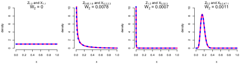
Figure 7: Density functions for $Z_{\rho,\delta}\sim F_{\rho,\delta}$ (pink) and $X_{\alpha_{3},\beta_{3}}\sim\mathrm{Beta}\left(\alpha_{3},\beta_{3}\right)$ (blue) for $\left(\rho,\delta\right)\in\left\{\left(1,0\right),\left(0.85,1.90\right),\left(1,5\right),\left(5,5\right)\right\}$ and $\alpha_{3}$, $\beta_{3}$ in (42) and (43). Putting $\left(\rho,\delta\right)\approx\left(0.85,1.90\right)$ maximizes the 2-Wasserstein distance between $Z_{\rho,\delta}$ and $X_{\alpha_{3},\beta_{3}}$ (see Figure 6). §2.4 proves convergence as $\rho$, $\nicefrac{{1}}{{\rho}}$, or $\left|\delta\right|$ grow large.

In sum, $\mathscr{L}\left(X_{\alpha_{3}\left(\rho,\delta\right),\beta_{3}\left(\rho,\delta\right)}\right)\approx\mathscr{L}\left(Z_{\rho,\delta}\right)$ for large or small $\rho$ or $\delta$ (Figure 7). In the sequel we use this approximation to approximate $\mathscr{L}\left(R_{0}\right)$ (Theorem 3.4). We then argue (from first principles) that our approximation of $\mathscr{L}\left(R_{0}\right)$ is exact as $\rho$ or $\delta$ become large or small (Theorem 3.6).

3 The (Approximate) Distribution of $R_{0}$

We here approximate the distribution of $R_{0}$, the rank of the odd normal out, using relationship (2) and mapping (42) and (43) (section 3.1). We show (from first principles) that our approximation and the true distribution approach each other as $\rho$ or $\delta$ become large or small. In section 3.2 we study the asymptotic distributions of the odd normal out as $\rho$ or $\delta$ become large or small.

3.1 Distribution and Moments

While Theorem 3.4 shows that the so-called beta-binomial distribution approximates $\mathscr{L}\left(R_{0}-1\right)$, we start by defining the beta-binomial distribution (Ng et al (2011) chapter 6) and describing its relevant characteristics.

Definition 3.1.

Let $X_{\alpha,\beta}\sim\mathrm{Beta}\left(\alpha,\beta\right)$ and $\left(\xi_{j}\left|X_{\alpha,\beta}\right.\right)\stackrel{{\scriptstyle\mathrm{iid}}}{{\sim}}\mathrm{Bernoulli}\left(X_{\alpha,\beta}\right)$, for $1\leq j\leq m$. Then, with

$$\left(Y_{m}\left|X_{\alpha,\beta}\right.\right)\coloneqq\sum_{j=1}^{m}\left(\xi_{j}\left|X_{\alpha,\beta}\right.\right)\sim\mathrm{Binomial}\left(m,X_{\alpha,\beta}\right)$$ (52)

we say that $Y_{m}$ has a beta-binomial distribution with parameters $\alpha,\beta,m$, which we abbreviate by writing $Y_{m}\sim\mathrm{BBinomial}\left(m,\alpha,\beta\right)$.

Lemma 3.2.

Letting Definition 3.1 define $Y_{m}$ and fixing $0\leq j\leq m$, we have

$$\Pr\left(Y_{m}=j\right) =\binom{m}{j}\frac{B\left(\alpha+j,\beta+m-j\right)}{B\left(\alpha,\beta\right)}$$ (53)

$$=\binom{m}{j}\frac{\Gamma\left(\alpha+j\right)\Gamma\left(\beta+m-j\right)}{\Gamma\left(\alpha+\beta+m\right)}\frac{\Gamma\left(\alpha+\beta\right)}{\Gamma\left(\alpha\right)\Gamma\left(\beta\right)}$$ (54)

where $B\left(\alpha,\beta\right)\coloneqq\int_{0}^{1}t^{\alpha-1}\left(1-t\right)^{\beta-1}dt$ and $\Gamma\left(\alpha\right)\coloneqq\int_{0}^{\infty}t^{\alpha-1}e^{-t}dt$ are the beta and gamma functions, for $\alpha,\beta>0$. Note that $B\left(\alpha,\beta\right)=\left.\Gamma\left(\alpha\right)\Gamma\left(\beta\right)\right/\Gamma\left(\alpha+\beta\right)$.

Proof.

Appendix E proves Lemma 3.2. ∎

Lemma 3.3.

Letting Definition 3.1 define $Y_{m}$ and $B_{m}\colonsim\mathrm{Binomial}\left(m,\mathbb{E}X_{\alpha,\beta}\right)$, we have

$$\mathbb{E}Y_{m} =\mathbb{E}B_{m}$$ (55)

$$\mathrm{Var}\left(Y_{m}\right) =\mathrm{Var}\left(B_{m}\right)\left[1+\left(m-1\right)\iota\right]$$ (56)

where $\iota\coloneqq\mathrm{Cor}\left(\xi_{1},\xi_{2}\right)=\nicefrac{{1}}{{\left(\alpha+\beta+1\right)}}\in\left(0,1\right)$ gives the so-called intra-class correlation. We consider three settings:

1. For $\alpha,\beta>0$ fixed, each $\xi_{j}$ depends on $X_{\alpha,\beta}$ and tends to increase as $X_{\alpha,\beta}$ increases, so that the $\left\{\xi_{j}\right\}$ are positively (but not perfectly) correlated.

2. If $\lim_{\alpha,\beta\rightarrow 0^{+}}\nicefrac{{\alpha}}{{\left(\alpha+\beta\right)}}\eqqcolon\lambda\in\left[0,1\right]$, then $Y_{m}$ converges in distribution to $m\mathrm{Bernoulli}\left(\lambda\right)$ as $\alpha,\beta\rightarrow 0^{+}$, so that the $\left\{\xi_{j}\right\}$ become perfectly correlated.

3. If $\lim_{\alpha,\beta\rightarrow\infty}\nicefrac{{\alpha}}{{\left(\alpha+\beta\right)}}\eqqcolon\lambda\in\left[0,1\right]$, then $Y_{m}$ converges in distribution to $\mathrm{Binomial}\left(m,\lambda\right)$ as $\alpha,\beta\rightarrow\infty$, so that the $\left\{\xi_{j}\right\}$ become independent.

Proof.

Appendix E proves Lemma 3.3. ∎

The above definitions and lemmas give key properties of $\mathrm{BBinomial}\left(m,\alpha,\beta\right)$. These in place, we state and prove this paper’s main result, the proof of which uses Lemma 3.2.

Theorem 3.4.

Say we have $n+1$ independent, normally-distributed random variables $X_{i}$, where $X_{0}\sim\mathcal{N}\left(\mu_{0},\sigma_{0}^{2}\right)$ and $X_{1},\ldots,X_{n}\sim\mathcal{N}\left(\mu,\sigma^{2}\right)$. For

$$R_{0}\coloneqq 1+\sum_{i=1}^{n}\mathbf{1}_{\left\{X_{i}\leq X_{0}\right\}}$$ (57)

the rank of the differently-distributed normal and $1\leq k\leq n+1$, we have

$$R_{0}\stackrel{{\scriptstyle\cdot}}{{\sim}}1+\mathrm{BBinomial}\left(n,\alpha_{3},\beta_{3}\right)$$ (58)

where $\alpha_{3}=\alpha_{3}\left(\rho,\delta\right)$ and $\beta_{3}=\beta_{3}\left(\rho,\delta\right)$ (with $\rho\coloneqq\nicefrac{{\sigma}}{{\sigma_{0}}}$ and $\delta\coloneqq\nicefrac{{\left(\mu-\mu_{0}\right)}}{{\sigma_{0}}}$) come from (42) and (43) and the dot above the $\sim$ symbol indicates approximation.

Proof.

Let $Y_{z}\sim\mathrm{Binomial}\left(n,z\right)$ and $Z_{\rho,\delta}\sim\Phi\left(\delta+\rho\Phi^{-1}\left(\cdot\right)\right)$. Then (2) gives

$$\Pr\left(R_{0}=k\right) =\Pr\left(Y_{Z_{\rho,\delta}}=k-1\right)$$ (59)

$$=\int_{0}^{1}\Pr\left(Y_{z}=k-1\right)f_{\rho,\delta}\left(z\right)dz$$ (60)

$$\approx\int_{0}^{1}\Pr\left(Y_{z}=k-1\right)b_{\alpha_{3},\beta_{3}}\left(z\right)dz$$ (61)

$$=\binom{n}{k-1}\frac{B\left(\alpha_{3}+k-1,\beta_{3}+n-k+1\right)}{B\left(\alpha_{3},\beta_{3}\right)}$$ (62)

where (61) assumes the argument of section 2.4 and (62) uses Lemma 3.2. ∎

Remark 3.5.

Comparing (3) and (62) we see that

$$\mathbb{E}\left[\Phi\left(\nicefrac{{\left(X_{0}-\mu\right)}}{{\sigma}}\right)^{k-1}\Phi\left(\nicefrac{{\left(\mu-X_{0}\right)}}{{\sigma}}\right)^{n+1-k}\right]\approx\frac{B\left(\alpha_{3}+k-1,\beta_{3}+n-k+1\right)}{B\left(\alpha_{3},\beta_{3}\right)}$$ (63)

Theorem 3.6 below shows that this relationship approaches equality as $\left|\delta\right|\rightarrow\infty$; as $\rho\rightarrow 0^{+}$; as $\rho\rightarrow\infty$; and as $\rho,\left|\delta\right|\rightarrow\infty$ while keeping $\nicefrac{{\delta}}{{\rho}}$ fixed.

The above result in hand, we now ask, how well does $1+\mathrm{BBinomial}\left(n,\alpha_{3},\beta_{3}\right)$ approximate $\mathscr{L}\left(R_{0}\right)$? Or, more specifically, one might ask, what is

$$W_{2}\left(1+\mathrm{BBinomial}\left(n,\alpha_{3},\beta_{3}\right),R_{0}\right)$$ (64)

where (32) defines $W_{2}$, as a function of $\rho$ and $\delta$? We do not compute (64) directly. Rather, we show that $W_{2}\left(1+\mathrm{BBinomial}\left(n,\alpha_{3},\beta_{3}\right),R_{0}\right)\rightarrow 0$ as $\left|\delta\right|\rightarrow\infty$; as $\rho\rightarrow 0^{+}$; as $\rho\rightarrow\infty$; and as $\rho,\left|\delta\right|\rightarrow\infty$ while keeping $\nicefrac{{\delta}}{{\rho}}$ fixed. To that end we let $p_{\rho,\delta}\left(k\right)$ represent the approximation in (61) and note that

$$\left|\Pr\left(R_{0}=k\right)-p_{\rho,\delta}\left(k\right)\right| \leq\int_{0}^{1}\Pr\left(Y_{z}=k-1\right)\left|f_{\rho,\delta}\left(z\right)-b_{\alpha_{3},\beta_{3}}\left(z\right)\right|dz$$ (65)

$$\leq\max_{0<z<1}\left|f_{\rho,\delta}\left(z\right)-b_{\alpha_{3},\beta_{3}}\left(z\right)\right|$$ (66)

where (65) uses (60)–(61). Now, if one can show that, for any $z\in\left(0,1\right)$,

$$\lim_{\left|\delta\right|\rightarrow\infty}\left\{f_{\rho,\delta}\left(z\right)-b_{\alpha_{3}\left(\rho,\delta\right),\beta_{3}\left(\rho,\delta\right)}\left(z\right)\right\} =0$$ (67)

$$\lim_{\rho\rightarrow 0^{+}}\left\{f_{\rho,\delta}\left(z\right)-b_{\alpha_{3}\left(\rho,\delta\right),\beta_{3}\left(\rho,\delta\right)}\left(z\right)\right\} =0$$ (68)

$$\lim_{\rho\rightarrow\infty}\left\{f_{\rho,\delta}\left(z\right)-b_{\alpha_{3}\left(\rho,\delta\right),\beta_{3}\left(\rho,\delta\right)}\left(z\right)\right\} =0$$ (69)

$$\lim_{\rho,\left|\delta\right|\rightarrow\infty}\left\{f_{\rho,\delta}\left(z\right)-b_{\alpha_{3}\left(\rho,\delta\right),\beta_{3}\left(\rho,\delta\right)}\left(z\right)\right\} =0$$ (70)

(the final limit keeps $\nicefrac{{\delta}}{{\rho}}$ fixed), (65)–(66) implies that $1+\mathrm{BBinomial}\left(n,\alpha_{3},\beta_{3}\right)$ and $\mathscr{L}\left(R_{0}\right)$ become the same distribution as (67) $\left|\delta\right|\rightarrow\infty$; (68) $\rho\rightarrow 0^{+}$; (69) $\rho\rightarrow\infty$; or (70) $\rho,\left|\delta\right|\rightarrow\infty$ while keeping $\nicefrac{{\delta}}{{\rho}}$ fixed. Limits (67)–(70) are easy to show in some cases, difficult in others.

Theorem 3.6.

$\mathscr{L}\left(R_{0}\right)$ and $1+\mathrm{BBinomial}\left(n,\alpha_{3},\beta_{3}\right)$ approach each other as $\left|\delta\right|\rightarrow\infty$; $\rho\rightarrow 0^{+}$; $\rho\rightarrow\infty$; or $\rho,\left|\delta\right|\rightarrow\infty$ while keeping $\nicefrac{{\delta}}{{\rho}}=r$ fixed.

Proof.

Appendix E proves Theorem 3.6. ∎

In the sequel we use the approximation and the limiting results in Theorems 3.4 and 3.6 to justify replacing $R_{0}$ with $R^{\prime}_{0}\sim\mathrm{BBinomial}\left(n,\alpha_{3},\beta_{3}\right)$. That said, we set these results aside for a moment, taking up instead the direct computation of $\mathbb{E}R_{0}$ and $\mathrm{Var}\left(R_{0}\right)$.

Proposition 3.7.

With $R_{0}\coloneqq 1+\sum_{i=1}^{n}\mathbf{1}_{\left\{X_{i}\leq X_{0}\right\}}$, we have

$$\mathbb{E}R_{0} =1+n\Phi\left(\nicefrac{{-\delta}}{{\sqrt{\rho^{2}+1}}}\right)\textrm{ and}$$ (71)

$$\mathrm{Var}\left(R_{0}\right) =n\Phi\left(\nicefrac{{-\delta}}{{\sqrt{\rho^{2}+1}}}\right)\Phi\left(\nicefrac{{\delta}}{{\sqrt{\rho^{2}+1}}}\right)\left[1+\left(n-1\right)\iota_{\rho,\delta}\right]$$ (72)

$$\textrm{where }\iota_{\rho,\delta} \coloneqq\left.\mathrm{Var}\left(Z_{\rho,\delta}\right)\right/\left[\Phi\left(\nicefrac{{-\delta}}{{\sqrt{\rho^{2}+1}}}\right)\Phi\left(\nicefrac{{\delta}}{{\sqrt{\rho^{2}+1}}}\right)\right]\in\left(0,1\right)$$ (73)

gives the intra-class correlation between $\mathbf{1}_{\left\{X_{1}\leq X_{0}\right\}}$ and $\mathbf{1}_{\left\{X_{2}\leq X_{0}\right\}}$ (Lemma 3.3).

Proof.

Appendix E proves Proposition 3.7. ∎

Remark 3.8.

Note that:

1. While (71)–(73) match (58) and Lemma 3.3, their derivation does not use them, but proceeds from first principles. Like the mapping (42)–(43) which provides (58), (58) preserves first and second moments.

2. $\mathrm{Var}\left(R_{0}\right)$ (72) and $\iota_{\rho,\delta}$ (73) are symmetric in $\delta$ about zero (Corollary 2.6).

3. The shape of $\left(\rho,\delta\right)\mapsto\mathrm{Var}\left(R_{0}\right)$ mimics that of $\left(\rho,\delta\right)\mapsto\mathrm{Var}\left(Z_{\rho,\delta}\right)$ (Figures 3 and 13 and statement 2b in “Regarding $\mathrm{Var}\left(R_{0}\right)$ and $\mathrm{Var}\left(R_{1}\right)$” in section 4.1.3).

4. From Theorem 2.13 we note that $\mathrm{Var}\left(Z_{\rho,\delta}\right)=\mathrm{Cov}\left(\mathbf{1}_{\left\{X_{1}\leq X_{0}\right\}},\mathbf{1}_{\left\{X_{2}\leq X_{0}\right\}}\right)$$=\Pr\left(X_{1}\leq X_{0},X_{2}\leq X_{0}\right)-\Pr\left(X_{1}\leq X_{0}\right)\Pr\left(X_{2}\leq X_{0}\right)$.

Corollary 3.9.

$\mathbb{E}R_{0}$, $\iota_{\rho,\delta}$, and $\mathrm{Var}\left(R_{0}\right)$ approach the limits tabulated below as $\rho\rightarrow 0^{+}$; $\rho\rightarrow\infty$; $\rho,\left|\delta\right|\rightarrow\infty$ while keeping $\nicefrac{{\delta}}{{\rho}}=r$ fixed; and $\left|\delta\right|\rightarrow\infty$.

	$\rho\rightarrow 0^{+}$	$\rho\rightarrow\infty$	$\rho,\left|\delta\right|\stackrel{{\scriptstyle[}}{{\mathrm{}}}{fixed}]{\nicefrac{{\delta}}{{\rho=r}}}{\longrightarrow}\infty$	$\delta\rightarrow\infty$	$\delta\rightarrow-\infty$
$\mathbb{E}R_{0}$	$n\Phi\left(-\delta\right)+1$	$\nicefrac{{n}}{{2}}+1$	$n\Phi\left(-r\right)+1$	$1$	$n+1$
$\iota_{\rho,\delta}$	$1$	$0$	$0$	$0$	$0$
$\mathrm{Var}\left(R_{0}\right)$	$n^{2}\Phi\left(-\delta\right)\Phi\left(\delta\right)$	$\nicefrac{{n}}{{4}}$	$n\Phi\left(-r\right)\Phi\left(r\right)$	$0$	$0$

Proof.

Appendix E proves Corollary 3.9. ∎

To summarize, we see that:

1. When $\mu_{0}\ll\mu$ (or, $\mu_{0}\gg\mu$), the rank of $X_{0}$ approaches 1 (or, $n+1$) in probability. In limit the $\left\{\mathbf{1}_{\left\{X_{i}\leq X_{0}\right\}}\right\}_{1}^{n}$ become uncorrelated as each one approaches 0 (or, 1) in probability. Section 3.2 proves this.

2. When $\sigma_{0}\gg\sigma$, $\mathrm{Var}\left(R_{0}\right)=\mathcal{O}\left(n^{2}\right)$. In fact, as we prove in section 3.2, $R_{0}\Longrightarrow 1+n\mathrm{Bernoulli}\left(\Phi\left(-\delta\right)\right)$, where $\Longrightarrow$ indicates convergence in distribution as $\rho\rightarrow 0^{+}$. That is to say, in this setting, we flip a $\Phi\left(-\delta\right)$-coin and place $X_{0}$ either above or below the $\left\{X_{i}\right\}_{1}^{n}$ depending on the outcome.

3. In the opposite setting, when $\sigma_{0}\ll\sigma$, $X_{0}$ tends to fall near the center of the $\left\{X_{i}\right\}_{1}^{n}$ and $\mathrm{Var}\left(R_{0}\right)=\mathcal{O}\left(n\right)$. We show in the sequel that $R_{0}\Longrightarrow 1+\mathrm{Binomial}\left(n,\nicefrac{{1}}{{2}}\right)$, where $\Longrightarrow$ indicates convergence in distribution as $\rho\rightarrow\infty$. In the limit, as $\rho\rightarrow\infty$, the $\left\{\mathbf{1}_{\left\{X_{i}\leq X_{0}\right\}}\right\}_{1}^{n}$ become independent and therefore uncorrelated (Lemma 3.3).

4. In the setting where $\rho,\left|\delta\right|\rightarrow\infty$, but $\nicefrac{{\delta}}{{\rho}}=r$ remains fixed, $X_{0}$ tends to be larger than $100\Phi\left(-r\right)\%$ of the $\left\{X_{i}\right\}_{1}^{n}$ and $\mathrm{Var}\left(R_{0}\right)=\mathcal{O}\left(n\right)$. Furthermore, as we show in the next section, $R_{0}\Longrightarrow 1+\mathrm{Binomial}\left(n,\Phi\left(-r\right)\right)$, where $\Longrightarrow$ indicates convergence in distribution as $\rho,\left|\delta\right|\rightarrow\infty$ while $\nicefrac{{\delta}}{{\rho}}=r$ remains fixed. In the limit the $\left\{\mathbf{1}_{\left\{X_{i}\leq X_{0}\right\}}\right\}_{1}^{n}$ become independent and therefore uncorrelated (Lemma 3.3).

Note that approximation (58) gives $R_{0}\sim\mathrm{Uniform}\left\{1,2,\ldots,n+1\right\}$ when $\mu=\mu_{0}$ and $\sigma=\sigma_{0}$ (so that $\alpha_{3}\left(1,0\right)=\beta_{3}\left(1,0\right)=1$). While the i.i.d. setting gives one the luxury of not thinking about the dependence between the $\left\{\mathbf{1}_{\left\{X_{i}\leq X_{0}\right\}}\right\}_{1}^{n}$, our complicated—but general—approach gives the correct answer in the i.i.d. setting. Approximation (58) gives the true distribution in this setting because $\mathscr{L}\left(Z_{1,0}\right)=\mathscr{L}\left(X_{1,1}\right)=\mathrm{Uniform}\left(0,1\right)$.

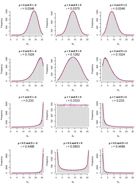
Figure 8: Simulated $R_{0}$ along with an approximation of $\mathscr{L}\left(R_{0}\right)$. Each panel represents some pair $\left(\rho,\delta\right)\in\left\{\nicefrac{{1}}{{2}},1,2,4\right\}\times\left\{-2,0,2\right\}$, provides a histogram of $10^{4}$ $R_{0}$ values, and gives the intra-class correlation $\iota_{\rho,\delta}$ in (73). Each $R_{0}$ uses $X_{0}\sim\mathcal{N}\left(0,1\right)$ and, independently, $X_{1},X_{2},\ldots,X_{25}$ i.i.d. $\mathcal{N}\left(\delta,\rho^{2}\right)$. The dotted pink curve gives (62) for $1\leq k\leq 26$, approximating $\mathscr{L}\left(R_{0}\right)$. The solid black curve gives the true distribution by approximating the integral in (60).

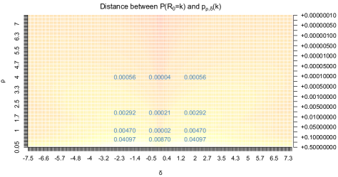
Figure 9: The 1-Wasserstein distance (74) between true distribution (60) and approximation (58). Gray numbers specify the distances between the black and pink distributions in Figure 8, with light blue circles highlighting the parameter combinations there. The color scale, chosen to highlight the shape of the surface, is log-linear with cut points at $\left\{1.0,2.5,5.0,7.5\right\}\times 10^{-j}$, for $1\leq j\leq 7$.

Figures 8 and 9 compare the true distribution of $R_{0}$ with approximation (58). Figure 8 simulates $10^{4}$ $R_{0}$ values for each $\left(\rho,\delta\right)\in\left\{\nicefrac{{1}}{{2}},1,2,4\right\}\times\left\{-2,0,2\right\}$ with $n=25$. We obtain the black curves for $\mathscr{L}\left(R_{0}\right)$ by approximating the integral in (60). The pink curves—matching both the black curves for $\mathscr{L}\left(R_{0}\right)$ and the simulated data—give approximation (58). Figure 9, the 1-Wasserstein distance between $\mathscr{L}\left(R_{0}\right)$ in (60) and approximation (58) for $\left(\rho,\delta\right)\in\left(0,\nicefrac{{15}}{{2}}\right]\times\left[\nicefrac{{-15}}{{2}},\nicefrac{{15}}{{2}}\right]$, broadens the analysis. The $W_{1}$ distance between $X\sim F_{X}$ and $Y\sim F_{Y}$ is

$$W_{1}\left(X,Y\right) \coloneqq\int_{0}^{1}\left|F_{X}^{-1}\left(z\right)-F_{Y}^{-1}\left(z\right)\right|dz=\int_{-\infty}^{\infty}\left|F_{X}\left(z\right)-F_{X}\left(z\right)\right|dz$$ (74)

$$=\sum_{k=1}^{n+1}\left|\Pr\left(R_{0}\leq k\right)-\sum_{j=1}^{k}p_{\rho,\delta}\left(j\right)\right|\textrm{ in our discrete setting}$$ (75)

where (62) defines $p_{\rho,\delta}\left(j\right)$. Figure 9 shows that approximation (58) improves as $\left|\delta\right|\rightarrow\infty$ or $\rho\rightarrow\infty$. While it does not show approximation (58) improving as $\rho\rightarrow 0^{+}$, this holds as well (Theorem 3.6). The smallest displayed $\rho$ is $\rho=0.05$. Further, one might reasonably doubt the numerical stability of our computations of $W_{1}\left(Z_{\rho,\delta},X_{\alpha_{3}\left(\rho,\delta\right),\beta_{3}\left(\rho,\delta\right)}\right)$ as $\rho\rightarrow 0^{+}$.

3.2 The Asymptotics of $R_{0}$

The paragraph following Corollary 3.9 describes limiting results for $\mathscr{L}\left(R_{0}\right)$ as $\rho$ or $\delta$ become large or small. We prove these results below. In summary,

1. If $\left|\delta\right|$ alone becomes large, $R_{0}$ approaches a fixed value: 1 if $\delta\rightarrow\infty$; $n+1$ if $\delta\rightarrow-\infty$ (Proposition 3.10).

2. If $\rho\rightarrow 0^{+}$, $R_{0}$ approaches a shifted and scaled Bernoulli random variable: $R_{0}$ equals 1 with probability $\Phi\left(\delta\right)$ and $n+1$ with probability $\Phi\left(-\delta\right)$ (Proposition 3.11).

3. If $\rho\rightarrow\infty$ (and optionally $\delta=r\rho$), $R_{0}$ approaches a binomial distribution (Propositions 3.12 and 3.13). Standardized, the binomial approaches normality as $n\rightarrow\infty$.

Table 1 outlines these and two additional limits: the limits for $\rho\rightarrow 0^{+},\left|\delta\right|\rightarrow\infty$ (in either order). We note finally that, when $R_{0}\rightarrow c\in\left\{1,n+1\right\}$, it converges in probability (Theorem 7.2.4(a) of Grimmett & Stirzaker (2001)).

	$\delta\rightarrow-\infty$	$\delta\in\mathbb{R}$	$\delta\rightarrow\infty$
$\rho\rightarrow 0^{+}$	$n+1$	$1+n\mathrm{Bern}\left(\Phi\left(-\delta\right)\right)$	1
$\rho\in\left(0,\infty\right)$	$n+1$	$\sim$$1+\mathrm{BBin}\left(n,\alpha_{3},\beta_{3}\right)$	1
$\rho\rightarrow\infty$	$1+\mathrm{Bin}\left(n,\Phi\left(-r\right)\right)$	$1+\mathrm{Bin}\left(n,\nicefrac{{1}}{{2}}\right)$	$1+\mathrm{Bin}\left(n,\Phi\left(-r\right)\right)$

Table 1: Limiting, approximate distributions for the rank of the odd normal out (Propositions 3.10, 3.11, 3.12, 3.13). When $R_{0}\rightarrow c$, it converges in probability. When $\rho,\left|\delta\right|\rightarrow\infty$, we assume that $\nicefrac{{\delta}}{{\rho}}=r\in\mathbb{R}$ remains fixed. Theorems 3.4 and 3.6 approximate $\mathscr{L}\left(R_{0}\right)$ for $\left(\rho,\delta\right)\in\left(0,\infty\right)\times\mathbb{R}$; see the central cell of the table.

3.2.1 When $\left|\delta\right|\rightarrow\infty$

We start with $\mu_{0}\gg\mu$ or $\mu_{0}\ll\mu$. In this setting $R_{0}$ approaches a fixed value:

Proposition 3.10.

For $1\leq i\leq n$ we have the following convergence in probability: $\mathbf{1}_{\left\{X_{i}\leq X_{0}\right\}}\stackrel{{\scriptstyle[}}{{\infty}}]{\delta}{\longrightarrow}0$, $\mathbf{1}_{\left\{X_{i}\leq X_{0}\right\}}\stackrel{{\scriptstyle[}}{{-}}\infty]{\delta}{\longrightarrow}1$, $R_{0}\stackrel{{\scriptstyle[}}{{-}}\infty]{\delta}{\longrightarrow}1$, and $R_{0}\stackrel{{\scriptstyle[}}{{\infty}}]{\delta}{\longrightarrow}n+1$.

Proof.

Appendix F proves Proposition 3.10. ∎

In this setting the $\left\{X_{i}\right\}_{i=1}^{n}$ will all fall to one side of $X_{0}$: above if $\mu_{0}\gg\mu$, and below if $\mu_{0}\ll\mu$.

3.2.2 When $\rho\rightarrow 0^{+}$

We turn to the setting in which $\sigma_{0}^{2}\gg\sigma^{2}$. Lemma 3.3.2 gives:

Proposition 3.11.

$R_{0}\Longrightarrow 1+n\mathrm{Bernoulli}\left(\Phi\left(-\delta\right)\right)$, where $\Longrightarrow$ gives convergence in distribution as $\rho\rightarrow 0^{+}$. In this setting the $\left\{\mathbf{1}_{\left\{X_{0}\leq X_{i}\right\}}\right\}_{1}^{n}$ are perfectly correlated.

Proof.

Appendix F proves Proposition 3.11. ∎

As $\rho\rightarrow 0^{+}$, the $\mathbf{1}_{\left\{X_{i}\leq X_{0}\right\}}$ travel as a group (Lemma 3.3.2; Corollary 3.9). If a $\Phi\left(-\delta\right)$-coin turns up heads (or, tails), $X_{0}$ is larger (or, smaller) than the $\left\{X_{i}\right\}_{i=1}^{n}$. Note that smaller (or, larger) values of $\delta=\nicefrac{{\left(\mu-\mu_{0}\right)}}{{\sigma_{0}}}$ favor $R_{0}=n+1$ (or, $R_{0}=1$).

3.2.3 When $\rho\rightarrow\infty$

We turn to the setting in which $\sigma^{2}\gg\sigma_{0}^{2}$. Lemma 3.3.3 gives:

Proposition 3.12.

$R_{0}\Longrightarrow 1+\mathrm{Binomial}\left(n,\nicefrac{{1}}{{2}}\right)$, where $\Longrightarrow$ gives convergence in distribution as $\rho\rightarrow\infty$. In this setting the $\left\{\mathbf{1}_{\left\{X_{0}\leq X_{i}\right\}}\right\}_{1}^{n}$ are iid $\mathrm{Bernoulli}\left(\nicefrac{{1}}{{2}}\right)$.

Proof.

Appendix F proves Proposition 3.12. ∎

Proposition 3.12 implies that $R_{0}$ is approximately normal when $\min\left(n,\rho\right)$ is large. In particular, $R_{0}\stackrel{{\scriptstyle\cdot}}{{\sim}}\mathcal{N}\left(1+n\Phi\left(\nicefrac{{-\delta}}{{\sqrt{\rho^{2}+1}}}\right),n\Phi\left(\nicefrac{{-\delta}}{{\sqrt{\rho^{2}+1}}}\right)\Phi\left(\nicefrac{{\delta}}{{\sqrt{\rho^{2}+1}}}\right)\right)$. When $\rho\rightarrow\infty$, the $\left\{X_{i}\right\}_{i=1}^{n}$ become so variable that the events $\left\{X_{i}\leq X_{0}\right\}$ no longer depend on the value of $X_{0}$.

3.2.4 When $\rho,\left|\delta\right|\rightarrow\infty$ While $\nicefrac{{\delta}}{{\rho}}$ Remains Fixed

We finally consider the setting in which $\mu_{0}\gg\mu$ or $\mu_{0}\ll\mu$ and $\sigma_{0}^{2}\ll\sigma^{2}$ in such a way that $\frac{\delta}{\rho}=\frac{\mu-\mu_{0}}{\sigma_{0}}$ remains fixed. Another application of Lemma 3.3.3 gives:

Proposition 3.13.

$R_{0}\Longrightarrow 1+\mathrm{Binomial}\left(n,\Phi\left(-r\right)\right)$, where $\Longrightarrow$ gives convergence in distribution as $\rho,\left|\delta\right|\rightarrow\infty$ while $\nicefrac{{\delta}}{{\rho}}=r$ remains fixed. In this setting the $\left\{\mathbf{1}_{\left\{X_{0}\leq X_{i}\right\}}\right\}_{1}^{n}$ are iid $\mathrm{Bernoulli}\left(\Phi\left(-r\right)\right)$.

Proof.

Appendix F proves Proposition 3.13. ∎

Proposition 3.13 implies that $R_{0}$ is approximately normal when $\min\left(n,\rho,\left|\delta\right|\right)$ is large. In particular, $R_{0}\stackrel{{\scriptstyle\cdot}}{{\sim}}\mathcal{N}\left(1+n\Phi\left(\nicefrac{{-\delta}}{{\sqrt{\rho^{2}+1}}}\right),n\Phi\left(\nicefrac{{-\delta}}{{\sqrt{\rho^{2}+1}}}\right)\Phi\left(\nicefrac{{\delta}}{{\sqrt{\rho^{2}+1}}}\right)\right)$. The $\mathbf{1}_{\left\{X_{i}\leq X_{0}\right\}}$ approach independence as $\rho\rightarrow\infty$ or as $\rho,\left|\delta\right|\rightarrow\infty$. The common issue is $\rho\rightarrow\infty$. When this occurs, the $\left\{X_{i}\right\}_{i=1}^{n}$ become so variable that the events $\left\{X_{i}\leq X_{0}\right\}$ no longer depend on the value of $X_{0}$. Letting $\left|\delta\right|\rightarrow\infty$ simply adds to this effect.

4 Joint Distributions

Up to this point we have focussed on the rank of the odd normal out. We now broaden our gaze to include the other normals. We first study distributions and moments (§4.1). We then consider asymptotics in $\rho$, $\delta$, and $n$ (§4.2).

4.1 Distributions and Moments

We study the ways in which the distributions of subsets of ranks depend on

$$\rho\coloneqq\frac{\sigma}{\sigma_{0}}\coloneqq\sqrt{\frac{\mathrm{Var}\left(X_{1}\right)}{\mathrm{Var}\left(X_{0}\right)}},\quad\delta\coloneqq\frac{\mu-\mu_{0}}{\sigma_{0}}\coloneqq\frac{\mathbb{E}\left[X_{1}-X_{0}\right]}{\sqrt{\mathrm{Var}\left(X_{0}\right)}}$$ (76)

To that end, let $R_{i}\coloneqq\sum_{j=0}^{n}\mathbf{1}_{\left\{X_{j}\leq X_{i}\right\}}$ be the rank of $X_{i}$, for $0\leq i\leq n$. Then, for $1\leq m\leq n$ and $1\leq i_{1}<i_{2}<\cdots<i_{m}\leq n$, we derive $\mathscr{L}\left(R_{0},R_{i_{1}},\ldots,R_{i_{m}}\right)$ and $\mathscr{L}\left(R_{i_{1}},\ldots,R_{i_{m}}\right)$:

Theorem 4.1.

For $1\leq m\leq n$, $1\leq i_{1}<i_{2}<\cdots<i_{m}\leq n$, and distinct values $\left\{j_{0},j_{1},\ldots,j_{m}\right\}\subset\left\{1,2,\ldots,n+1\right\}$,

$$\Pr\left(R_{0}=j_{0},R_{i_{1}}=j_{1},\ldots,R_{i_{m}}=j_{m}\right) =\frac{\Pr\left(R_{0}=j_{0}\right)}{n\left(n-1\right)\cdots\left(n-m+1\right)}$$ (77)

$$\Pr\left(R_{i_{1}}=j_{1},R_{i_{2}}=j_{2},\ldots,R_{i_{m}}=j_{m}\right) =\frac{1-\sum_{k=1}^{m}\Pr\left(R_{0}=j_{k}\right)}{n\left(n-1\right)\cdots\left(n-m+1\right)}$$ (78)

so that

$$\mathbb{E}R_{1} =\frac{n+1}{2}+\Phi\left(\nicefrac{{\delta}}{{\sqrt{\rho^{2}+1}}}\right)$$ (79)

$$\mathrm{Var}\left(R_{1}\right) =\frac{n^{2}-1}{12}+n\Phi\left(\nicefrac{{-\delta}}{{\sqrt{\rho^{2}+1}}}\right)\Phi\left(\nicefrac{{\delta}}{{\sqrt{\rho^{2}+1}}}\right)-\left(n-1\right)\mathrm{Var}\left(Z_{\rho,\delta}\right)$$ (80)

$$\mathrm{Cov}\left(R_{0},R_{1}\right) =-\Phi\left(\nicefrac{{-\delta}}{{\sqrt{\rho^{2}+1}}}\right)\Phi\left(\nicefrac{{\delta}}{{\sqrt{\rho^{2}+1}}}\right)-\left(n-1\right)\mathrm{Var}\left(Z_{\rho,\delta}\right)$$ (81)

$$\mathrm{Cov}\left(R_{1},R_{2}\right) =-\frac{n+1}{12}-\Phi\left(\nicefrac{{-\delta}}{{\sqrt{\rho^{2}+1}}}\right)\Phi\left(\nicefrac{{\delta}}{{\sqrt{\rho^{2}+1}}}\right)+2\mathrm{Var}\left(Z_{\rho,\delta}\right)$$ (82)

where Theorem 2.13 gives $\mathrm{Var}\left(Z_{\rho,\delta}\right)$.

Proof.

Appendix G proves Theorem 4.1. ∎

In what follows let

$$\mathrm{Cor}\left(R_{0},R_{1}\right)\coloneqq\frac{\mathrm{Cov}\left(R_{0},R_{1}\right)}{\sqrt{\mathrm{Var}\left(R_{0}\right)\mathrm{Var}\left(R_{1}\right)}},\quad\mathrm{Cor}\left(R_{1},R_{2}\right)\coloneqq\frac{\mathrm{Cov}\left(R_{1},R_{2}\right)}{\mathrm{Var}\left(R_{1}\right)}$$ (83)

so that $\mathrm{Cov}\left(R_{0},R_{1}\right)$ and $\mathrm{Cor}\left(R_{0},R_{1}\right)$ give the covariance and correlation between the odd normal out and any in-normal, and $\mathrm{Cov}\left(R_{1},R_{2}\right)$ and $\mathrm{Cor}\left(R_{1},R_{2}\right)$ give the covariance and correlation between any two in-normals. Note also that $\mathbb{E}R_{i}=\mathbb{E}R_{1}$ and $\mathrm{Var}\left(R_{i}\right)=\mathrm{Var}\left(R_{1}\right)$, for $1\leq i\leq n$, because $\mathscr{L}\left(R_{i}\right)=\mathscr{L}\left(R_{j}\right)$ for $1\leq i,j\leq n$.

Corollary 4.2.

$\mathbb{E}R_{1}$, $\mathrm{Var}\left(R_{1}\right)$, $\mathrm{Cov}\left(R_{0},R_{1}\right)$, $\mathrm{Cov}\left(R_{1},R_{2}\right)$, $\mathrm{Cor}\left(R_{0},R_{1}\right)$, and $\mathrm{Cor}\left(R_{1},R_{2}\right)$ approach the limits tabulated below as $\rho\rightarrow 0^{+}$; $\rho\rightarrow\infty$; $\rho,\left|\delta\right|\rightarrow\infty$ while keeping $\nicefrac{{\delta}}{{\rho}}=r$ fixed; and $\left|\delta\right|\rightarrow\infty$.^,

$\rho\rightarrow 0^{+}$ $\rho\rightarrow\infty$ $\rho,\left|\delta\right|\stackrel{{\scriptstyle[}}{{\mathrm{}}}{fixed}]{\nicefrac{{\delta}}{{\rho=r}}}{\longrightarrow}\infty$ $\delta\rightarrow\infty$ $\delta\rightarrow-\infty$ $\mathbb{E}R_{0}$ $n\Phi\left(-\delta\right)+1$ $\frac{n}{2}+1$ $n\Phi\left(-r\right)+1$ $1$ $n+1$ $\mathbb{E}R_{1}$ $\frac{n+1}{2}+\Phi\left(\delta\right)$ $\frac{n}{2}+1$ $\frac{n+1}{2}+\Phi\left(r\right)$ $\frac{n+3}{2}$ $\frac{n+1}{2}$ $\mathrm{Var}\left(R_{0}\right)$ $n^{2}\Phi\left(-\delta\right)\Phi\left(\delta\right)$ $\frac{n}{4}$ $n\Phi\left(-r\right)\Phi\left(r\right)$ $0$ $0$ $\mathrm{Var}\left(R_{1}\right)$ $\frac{n^{2}-1}{12}+\Phi\left(-\delta\right)\Phi\left(\delta\right)$ $\frac{n^{2}-1}{12}+\frac{n}{4}$ $\frac{n^{2}-1}{12}+n\Phi\left(-r\right)\Phi\left(r\right)$ $\frac{n^{2}-1}{12}$ $\frac{n^{2}-1}{12}$ $\mathrm{Cov}\left(R_{0},R_{1}\right)$ $-n\Phi\left(-\delta\right)\Phi\left(\delta\right)$ $-\frac{1}{4}$ $-\Phi\left(-r\right)\Phi\left(r\right)$ $0$ $0$ $\mathrm{Cov}\left(R_{1},R_{2}\right)$ $-\frac{n+1}{12}+\Phi\left(-\delta\right)\Phi\left(\delta\right)$ $-\frac{n+1}{12}-\frac{1}{4}$ $-\frac{n+1}{12}-\Phi\left(-r\right)\Phi\left(r\right)$ $-\frac{n+1}{12}$ $-\frac{n+1}{12}$ $\mathrm{Cor}\left(R_{0},R_{1}\right)$ $-\sqrt{\frac{12\Phi\left(-\delta\right)\Phi\left(\delta\right)}{n^{2}+12\Phi\left(-\delta\right)\Phi\left(\delta\right)-1}}$ $-\sqrt{\frac{3}{n^{3}+3n^{2}-n}}$ $-\sqrt{\frac{12\Phi\left(-r\right)\Phi\left(r\right)}{n^{3}+12\Phi\left(-r\right)\Phi\left(r\right)n^{2}-n}}$ $\mathtt{NaN}$ $\mathtt{NaN}$ $\mathrm{Cor}\left(R_{1},R_{2}\right)$ $-\frac{n-12\Phi\left(-\delta\right)\Phi\left(\delta\right)+1}{n^{2}+12\Phi\left(-\delta\right)\Phi\left(\delta\right)-1}$ $-\frac{n+4}{n^{2}+3n-1}$ $-\frac{n+12\Phi\left(-r\right)\Phi\left(r\right)+1}{n^{2}+12n\Phi\left(-r\right)\Phi\left(r\right)-1}$ $-\frac{1}{n-1}$ $-\frac{1}{n-1}$

Proof.

See (79) through (83) and Corollary 3.9. ∎

While Theorem 4.1 gives six key formulae, Corollary 4.2 gives forty limiting results. The following definitions help us make sense of the results above.

Definition 4.3.

For $i\leq j$, $i\textrm{:}j\coloneqq\left\{i,i+1,\ldots,j\right\}$, and $k\leq m\coloneqq j-i+1$, let

$$\mathcal{S}_{i\textrm{:}j,k}\coloneqq\left\{\mathbf{l}\in\left(i\textrm{:}j\right)^{k}:l_{1},l_{2},\ldots,l_{k}\textrm{ all distinct}\right\}$$ (84)

be the set of vectors from $\left(i\textrm{:}j\right)^{k}$ with unique elements. When $i=1$, we write $\mathcal{S}_{j,k}\coloneqq\mathcal{S}_{1\textrm{:}j,k}$. Note that $\left|\mathcal{S}_{i\textrm{:}j,k}\right|=\Pi_{l=1}^{k}\left(m-l+1\right)$, and that, for $k\geq 2$, $\mathbf{U}\sim\mathrm{Uniform}\left(\mathcal{S}_{i\textrm{:}j,k}\right)$ gives $\left(U_{1},U_{2},\ldots,U_{k-1}\right)\sim\mathrm{Uniform}\left(\mathcal{S}_{i\textrm{:}j,k-1}\right)$. Note also that

$$\begin{array}[]{rrr}\mathbb{E}U_{1}=\frac{i+j}{2},&&\mathrm{Cov}\left(U_{1},U_{2}\right)=-\frac{m+1}{12}\\ \mathrm{Var}\left(U_{1}\right)=\frac{m^{2}-1}{12},&&\mathrm{Cor}\left(U_{1},U_{2}\right)=-\frac{1}{m-1}\end{array}$$ (85)

Definition 4.4.

Let $\mathbf{R}\coloneqq\left(R_{0},R_{1},\ldots,R_{n}\right)^{\mathsf{T}}$ be the vector of ranks, so that $\mathbb{E}\mathbf{R}$ gives the vector of expected ranks and $\mathrm{Var}\left(\mathbf{R}\right)$ gives the variance-covariance matrix for the ranks. Letting $\mathbf{1}_{m}$ be the vector of ones in $\mathbb{R}^{m}$, we note that

$$\mathbb{E}\mathbf{R} =\left[\begin{array}[]{c}1+n\Phi\left(\nicefrac{{-\delta}}{{\sqrt{\rho^{2}+1}}}\right)\\ \left(\frac{n+1}{2}+\Phi\left(\nicefrac{{\delta}}{{\sqrt{\rho^{2}+1}}}\right)\right)\mathbf{1}_{n}\end{array}\right]$$ (88)

$$\mathrm{Var}\left(\mathbf{R}\right) =\left[\begin{array}[]{cc}\mathrm{Var}\left(R_{0}\right)&\mathrm{Cov}\left(R_{0},R_{1}\right)\mathbf{1}_{n}^{\mathsf{T}}\\ \mathrm{Cov}\left(R_{0},R_{1}\right)\mathbf{1}_{n}&\boldsymbol{\Sigma}_{1:n}\end{array}\right]$$ (91)

where $\boldsymbol{\Sigma}_{1:n}\coloneqq\mathrm{Cov}\left(R_{1},R_{2}\right)\mathbf{1}_{n}\mathbf{1}_{n}^{\mathsf{T}}+\mathrm{diag}\left[\left(\mathrm{Var}\left(R_{1}\right)-\mathrm{Cov}\left(R_{1},R_{2}\right)\right)\mathbf{1}_{n}\right]$ and, for $\mathbf{v}\in\mathbb{R}^{m}$, $\mathrm{diag}\left(\mathbf{v}\right)\in\mathbb{R}^{m\times m}$ is the matrix with $\mathbf{v}$ on the main diagonal and zeros elsewhere (Proposition 3.7; Theorem 4.1). Note that $\Pr\left(\mathbf{R}\in\mathcal{S}_{n+1,n+1}\right)=1$ as

$$\mathbf{X}\sim\mathcal{N}_{n+1}\left(\left(\begin{array}[]{c}\mu_{0}\\ \mu\mathbf{1}_{n}\end{array}\right),\left(\begin{array}[]{cc}\sigma_{0}^{2}&\mathbf{0}_{n}^{\mathsf{T}}\\ \mathbf{0}_{n}&\mathrm{diag}\left(\sigma^{2}\mathbf{1}_{n}\right)\end{array}\right)\right)$$ (92)

for $\mathbf{X}\coloneqq\left(X_{0},X_{1},\ldots,X_{n}\right)$ and $\mathbf{0}_{m}$ the vector of zeros in $\mathbb{R}^{m}$. The $\left\{R_{i}\right\}_{i=0}^{n}$ do not inherit the independence of the $\left\{X_{i}\right\}_{i=0}^{n}$. Finally, the correlation matrix is

$$\mathrm{Cor}\left(\mathbf{R}\right)=\left[\begin{array}[]{cc}1&\mathrm{Cor}\left(R_{0},R_{1}\right)\mathbf{1}_{n}^{\mathsf{T}}\\ \mathrm{Cor}\left(R_{0},R_{1}\right)\mathbf{1}_{n}&\boldsymbol{\Xi}_{1:n}\end{array}\right]$$ (93)

where $\boldsymbol{\Xi}_{1:n}\coloneqq\mathrm{Cor}\left(R_{1},R_{2}\right)\mathbf{1}_{n}\mathbf{1}_{n}^{\mathsf{T}}+\mathrm{diag}\left[\left(1-\mathrm{Cor}\left(R_{1},R_{2}\right)\right)\mathbf{1}_{n}\right]$ (Theorem 4.1).

With these concepts in place, the sections that follow consider distributions $\mathscr{L}\left(R_{0},R_{i_{1}},\ldots,R_{i_{m}}\right)$ and $\mathscr{L}\left(R_{i_{1}},\ldots,R_{i_{m}}\right)$ (§4.1.1), the mean $\mathbb{E}\mathbf{R}$ (§4.1.2), and the covariance and correlation matrices $\mathrm{Var}\left(\mathbf{R}\right)$ and $\mathrm{Cor}\left(\mathbf{R}\right)$ (§4.1.3).

4.1.1 Distributions $\mathscr{L}\left(R_{0},R_{i_{1}},\ldots,R_{i_{m}}\right)$ and $\mathscr{L}\left(R_{i_{1}},\ldots,R_{i_{m}}\right)$

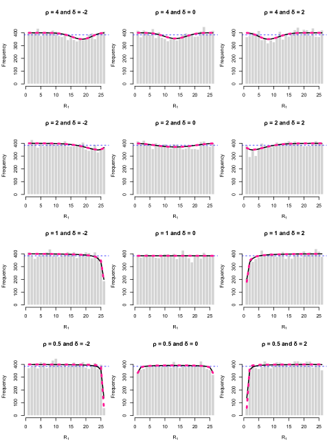
Figure 10: Simulated $R_{1}$ with $\mathscr{L}\left(R_{1}\right)$ and an approximation of $\mathscr{L}\left(R_{1}\right)$. Each panel represents a pair $\left(\rho,\delta\right)\in\left\{\nicefrac{{1}}{{2}},1,2,4\right\}\times\left\{-2,0,2\right\}$, providing a histogram of $10^{4}$ ranks $R_{1}$. Each independent $R_{1}$ uses $X_{0}\sim\mathcal{N}\left(0,1\right)$ and, independently, $X_{1},X_{2},\ldots,X_{25}$ i.i.d. $\mathcal{N}\left(\delta,\rho^{2}\right)$. The dotted pink curves approximate $\mathscr{L}\left(R_{1}\right)$ using (78) and (61). The black curves give the true distribution using (78) and (60). The dotted blue lines give expected counts under $\mathrm{Uniform}\left\{1,2,\ldots,26\right\}$.

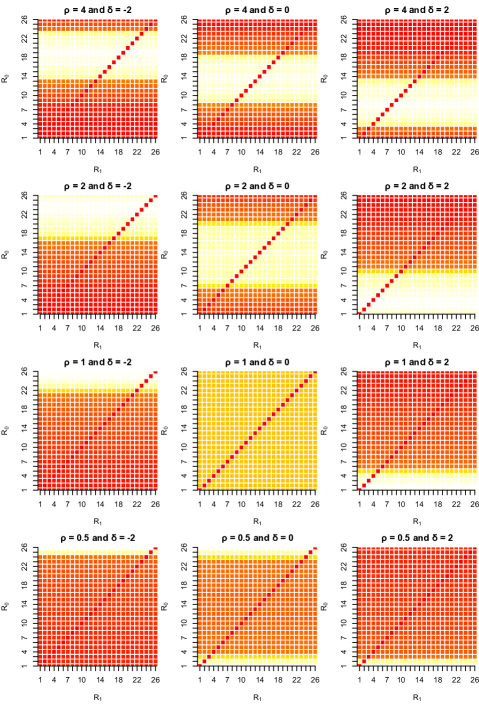
Figure 11: The distribution $\mathscr{L}\left(R_{0},R_{1}\right)$ when $n=25$ for $\left(\rho,\delta\right)\in\left\{\nicefrac{{1}}{{2}},1,2,4\right\}\times\left\{-2,0,2\right\}$. Colors match those in Figure 12: red=small values (0 when $R_{0}=R_{1}$) and white=large values. We calculate probabilities using (77) and (60).

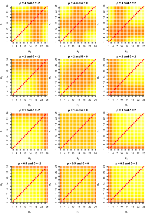
Figure 12: The distribution $\mathscr{L}\left(R_{1},R_{2}\right)$ when $n=25$ for $\left(\rho,\delta\right)\in\left\{\nicefrac{{1}}{{2}},1,2,4\right\}\times\left\{-2,0,2\right\}$. Colors match those in Figure 11: red=small values (0 when $R_{1}=R_{2}$) and white=large values. We calculate probabilities using (78) and (60).

Figures 10, 11, and 12 show $\mathscr{L}\left(R_{1}\right)$, $\mathscr{L}\left(R_{0},R_{1}\right)$, and $\mathscr{L}\left(R_{1},R_{2}\right)$ when $n=25$ and $\left(\rho,\delta\right)\in\left\{\nicefrac{{1}}{{2}},1,2,4\right\}\times\left\{-2,0,2\right\}$. In what follows we highlight some of the messages these figures convey. We first consider $\mathscr{L}\left(R_{1}\right)$. With $\Pr\left(R_{1}=k\right)=\frac{1}{n}\left[1-\Pr\left(R_{0}=k\right)\right]$, $\mathscr{L}\left(R_{1}\right)$ is the photographic negative of $\mathscr{L}\left(R_{0}\right)$ relative to a uniform baseline. When $\left(\rho,\delta\right)\neq\left(1,0\right)$, $R_{1}$ ebbs towards the ranks that $R_{0}$—in a manner of speaking—does not want.

Figures 11 and 12 show this in the two-dimensional setting. Figure 12 shows $R_{1}$ and $R_{2}$ moving away from areas where $\Pr\left(R_{0}=k\right)$ is large. Figure 11 shows an otherwise flat surface rolling up and down with $\Pr\left(R_{0}=k\right)$. Specifically,

$$\left(\left.R_{1}\right|R_{0}\right)\sim\mathrm{Uniform}\left(\left.\left\{1,2,\ldots,n+1\right\}\right\backslash\left\{R_{0}\right\}\right)$$ (94)

gives $\Pr\left(R_{0}=j,R_{1}=k\right)=\frac{1}{n}\Pr\left(R_{0}=j\right)$, for $\left(j,k\right)\in\mathcal{S}_{n+1,2}$.

Each panel of Figure 10 shows $10^{4}$ simulated $R_{1}$ values. Each independent $R_{1}$ uses $X_{0}\sim\mathcal{N}\left(0,1\right)$ and, independently, $X_{1},X_{2},\ldots,X_{25}$ i.i.d. $\mathcal{N}\left(\delta,\rho^{2}\right)$. Black curves use (78) with $m=1$ and then approximate integral (60). Pink curves use (78) with $m=1$ and the beta-binomial approximation for $\mathscr{L}\left(R_{0}-1\right)$ in (61). The pink and black curves show a strong overlap, an overlap that increases as $\rho$ increases (Proposition 3.12). Furthermore, both mirror the simulated ranks.

4.1.2 Mean $\mathbb{E}\mathbf{R}$

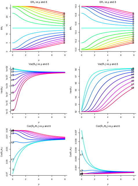
Figure 13: Means, variances, and correlations for $R_{0},R_{1},R_{2}$ (Proposition 3.7; Theorem 4.1). The $y$-axis gives the parameter. (The $\mathrm{Var}\left(R_{0}\right)$ panel uses the log scale.) The $x$-axis gives $0<\rho\leq 8$. Curve color gives $\delta\in\left\{-8,-7,\ldots,8\right\}$. Labels indicate which curve is which. Variances and correlations are symmetric in $\delta$ about 0; e.g., $\mathrm{Var}_{\rho,\delta}\left(R_{0}\right)=\mathrm{Var}_{\rho,-\delta}\left(R_{0}\right)$. Corollary 4.2 identifies the limits of these curves (and also the covariance curves) as $\rho$ or $\delta$ grow large or small.

With $\mathbf{1}_{m}$ the vector of ones in $\mathbb{R}^{m}$, we have

$$\mathbb{E}\mathbf{R}=\left[\begin{array}[]{c}1+n\Phi\left(\nicefrac{{-\delta}}{{\sqrt{\rho^{2}+1}}}\right)\\ \left(\frac{n+1}{2}+\Phi\left(\nicefrac{{\delta}}{{\sqrt{\rho^{2}+1}}}\right)\right)\mathbf{1}_{n}\end{array}\right]$$ (95)

as in Definition 4.4. From this we note that:

1. For $0\leq j\leq n$, $\left(\nicefrac{{n}}{{2}}+1\right)-\mathbb{E}_{\rho,\delta}R_{j}=\mathbb{E}_{\rho,-\delta}R_{j}-\left(\nicefrac{{n}}{{2}}+1\right)$. Flipping the sign of $\delta$ reflects $\mathbb{E}_{\rho,\delta}R_{j}$ about $\lim_{\rho\rightarrow\infty}\mathbb{E}_{\rho,\delta}R_{j}=\nicefrac{{n}}{{2}}+1=\mathbb{E}\mathrm{Uniform}\left(\mathcal{S}_{n+1,1}\right)$, the balance point among equally-weighted ranks (see Figure 13, Corollary 4.2, and Definition 4.3).

2. As $\rho$ increases, if $\delta>0$ (or, $\delta<0$), $\mathbb{E}R_{0}$ approaches $\nicefrac{{n}}{{2}}+1$ from below (or, from above) while $\mathbb{E}R_{1}$ approaches $\nicefrac{{n}}{{2}}+1$ from above (or, from below). See Figure 13 and Corollary 4.2.

3. $\mathbb{E}R_{0}$ varies in $\rho$ and $\delta$ across $\left(1,n+1\right)$ while $\mathbb{E}R_{1}$ varies across $\left(\frac{n+1}{2},\frac{n+3}{2}\right)$. This is not surprising. Note that $\mathbb{E}R_{1}=\mathbb{E}\mathrm{Uniform}\left(\mathcal{S}_{n,1}\right)+\Pr\left(X_{0}<X_{1}\right)$ (Theorem 2.8 and Proposition 4.6).

4. As expected, $\sum_{i=0}^{n}\mathbb{E}R_{i}=\nicefrac{{\left(n+1\right)\left(n+2\right)}}{{2}}=\sum_{k=1}^{n+1}k$, the sum of the ranks.

4.1.3 Covariance and Correlation Matrices $\mathrm{Var}\left(\mathbf{R}\right)$ and $\mathrm{Cor}\left(\mathbf{R}\right)$

With $\mathbf{1}_{m}$ the vector of ones in $\mathbb{R}^{m}$, the covariance and correlation matrices are

$$\mathrm{Var}\left(\mathbf{R}\right) =\left[\begin{array}[]{cc}\mathrm{Var}\left(R_{0}\right)&\mathrm{Cov}\left(R_{0},R_{1}\right)\mathbf{1}_{n}^{\mathsf{T}}\\ \mathrm{Cov}\left(R_{0},R_{1}\right)\mathbf{1}_{n}&\boldsymbol{\Sigma}_{1:n}\end{array}\right]$$ (98)

$$\mathrm{Cor}\left(\mathbf{R}\right) =\left[\begin{array}[]{cc}1&\mathrm{Cor}\left(R_{0},R_{1}\right)\mathbf{1}_{n}^{\mathsf{T}}\\ \mathrm{Cor}\left(R_{0},R_{1}\right)\mathbf{1}_{n}&\boldsymbol{\Xi}_{1:n}\end{array}\right]$$ (101)

where

$$\boldsymbol{\Sigma}_{1:n} \coloneqq\mathrm{Cov}\left(R_{1},R_{2}\right)\mathbf{1}_{n}\mathbf{1}_{n}^{\mathsf{T}}+\mathrm{diag}\left[\left(\mathrm{Var}\left(R_{1}\right)-\mathrm{Cov}\left(R_{1},R_{2}\right)\right)\mathbf{1}_{n}\right]$$ (102)

$$\boldsymbol{\Xi}_{1:n} \coloneqq\mathrm{Cor}\left(R_{1},R_{2}\right)\mathbf{1}_{n}\mathbf{1}_{n}^{\mathsf{T}}+\mathrm{diag}\left[\left(1-\mathrm{Cor}\left(R_{1},R_{2}\right)\right)\mathbf{1}_{n}\right]$$ (103)

as in Definition 4.4. The following paragraphs consider $\mathrm{Var}\left(R_{1}\right)$, $\mathrm{Var}\left(R_{0}\right)$ and $\mathrm{Var}\left(R_{1}\right)$, and $\mathrm{Var}\left(\mathbf{R}\right)$ and $\mathrm{Cor}\left(\mathbf{R}\right)$ in turn.

Regarding $\mathrm{Var}\left(R_{1}\right)$

Ignoring terms of $\mathcal{O}\left(\nicefrac{{1}}{{n}}\right)$, we have, from (80),

$$\mathrm{Var}\left(R_{1}\right)\sim\left(1-\iota_{\rho,\delta}\right)\mathrm{Var}\left(B_{n}\right)+\mathrm{Var}\left(U_{n}\right)$$ (104)

for $B_{n}\sim\mathrm{Binomial}\left(n,\Phi\left(\nicefrac{{-\delta}}{{\sqrt{\rho^{2}+1}}}\right)\right)$, $U_{n}\sim\mathrm{Uniform}\left(\mathcal{S}_{n,1}\right)$, and the intra-class correlation $\iota_{\rho,\delta}\coloneqq\mathrm{Cor}\left(\mathbf{1}_{\left\{X_{1}\leq X_{0}\right\}},\mathbf{1}_{\left\{X_{1}\leq X_{0}\right\}}\right)\in\left(0,1\right)$. We note three settings:

1. When $\rho\rightarrow 0^{+}$, we have $\iota_{\rho,\delta}\rightarrow 1^{-}$ (Corollary 3.9) and $\mathrm{Var}\left(R_{1}\right)=\mathrm{Var}\left(U_{n}\right)$. In this setting, $R_{1}$’s variance does not reflect the coin flip that determines $R_{0}$’s value (Proposition 3.11), but does reflect $R_{1}$’s uniform selection from a set of $n$ consecutive integers (Proposition 4.6).

2. When $\rho\rightarrow\infty$ or $\rho,\left|\delta\right|\rightarrow\infty$ while keeping $\nicefrac{{\delta}}{{\rho}}=r$ fixed, we have $\iota_{\rho,\delta}\rightarrow 0^{+}$ (Corollary 3.9) and $\mathrm{Var}\left(B_{n}\right)\not\rightarrow 0$, so that $\mathrm{Var}\left(R_{1}\right)=\mathrm{Var}\left(U_{n}\right)+\mathrm{Var}\left(B_{n}\right)$. In this setting $\mathscr{L}\left(R_{0}\right)=\mathscr{L}\left(B_{n}\right)$ (Propositions 3.12 and 3.13). As usual $\left(R_{1}\left|R_{0}\right.\right)\sim\mathrm{Uniform}\left(\left.\mathcal{S}_{n+1,1}\right\backslash\left\{R_{0}\right\}\right)$ (see (94)). While

   $$\mathrm{Var}\left(\left.R_{1}\right|R_{0}\right)=\frac{n+1}{12n^{2}}\left[\left(n+2\right)\left(n^{2}-3n-6\right)+12R_{0}\left(n-R_{0}+2\right)\right]$$ (105)

   so that

   $$\mathrm{Var}\left(\left.R_{1}\right|R_{0}=j\right)\left\{\begin{array}[]{rl}=\mathrm{Var}\left(U_{n}\right)&\textrm{if }j\in\left\{1,n+1\right\}\\ >\mathrm{Var}\left(U_{n}\right)&\textrm{if }j\in\left\{2,3,\ldots,n\right\}\end{array}\right.$$ (106)

   $\mathrm{Var}\left(R_{1}\right)$ captures $R_{0}$’s selection along with a diminution of $R_{1}$’s selection given $R_{0}$.

3. When $\left|\delta\right|\rightarrow\infty$, we have $\iota_{\rho,\delta}\rightarrow 0^{+}$ (Corollary 3.9) and $\mathrm{Var}\left(B_{n}\right)\rightarrow 0$, leaving us with the reasonable $\mathrm{Var}\left(R_{1}\right)=\mathrm{Var}\left(U_{n}\right)$ (see Propositions 3.10 and 4.5).

Regarding $\mathrm{Var}\left(R_{0}\right)$ and $\mathrm{Var}\left(R_{1}\right)$

We show that $\mathrm{Var}\left(Z_{\rho,\delta}\right)$’s size relative to $\nicefrac{{1}}{{12}}$ determines $\mathrm{Var}\left(R_{0}\right)$’s size relative to $\mathrm{Var}\left(R_{1}\right)$. We then study $\mathrm{Var}\left(R_{0}\right)$ and $\mathrm{Var}\left(R_{1}\right)$’s relative dependence on the intra-class correlation $\iota_{\rho,\delta}\coloneqq\mathrm{Cor}\left(\mathbf{1}_{\left\{X_{1}\leq X_{0}\right\}},\mathbf{1}_{\left\{X_{2}\leq X_{0}\right\}}\right)\in\left(0,1\right)$, $\mathrm{Var}\left(Z_{\rho,\delta}\right)$, and the number of within-group normals $n$.

1. From Proposition 3.7 and Theorem 4.1 we see that

   $$\mathrm{Var}\left(R_{0}\right) =\mathrm{Var}\left(B_{n}\right)\left[1+\left(n-1\right)\iota_{\rho,\delta}\right]$$ (107)

   $$\mathrm{Var}\left(R_{1}\right) =\mathrm{Var}\left(B_{n}\right)\left[1-\left(n-1\right)\nicefrac{{\iota_{\rho,\delta}}}{{n}}\right]+\mathrm{Var}\left(U_{n}\right)$$ (108)

   for $B_{n}\sim\mathrm{Binomial}\left(n,\Phi\left(\nicefrac{{-\delta}}{{\sqrt{\rho^{2}+1}}}\right)\right)$, $U_{n}\sim\mathrm{Uniform}\left(\mathcal{S}_{n,1}\right)$, and inter-class correlation $\iota_{\rho,\delta}\coloneqq\mathrm{Cor}\left(\mathbf{1}_{\left\{X_{1}\leq X_{0}\right\}},\mathbf{1}_{\left\{X_{2}\leq X_{0}\right\}}\right)\in\left(0,1\right)$. This implies that

   $$\mathrm{Var}\left(R_{0}\right)\lesseqqgtr\mathrm{Var}\left(R_{1}\right)\Longleftrightarrow\mathrm{Var}\left(Z_{\rho,\delta}\right)\lesseqqgtr\nicefrac{{1}}{{12}}$$ (109)

   Propositions 2.10, 2.18, and 2.20 then imply that

   $$\left\{\left(\rho,\delta\right)\in\left(0,\infty\right)\times\mathbb{R}:\mathrm{Var}\left(R_{0}\right)>\mathrm{Var}\left(R_{1}\right)\right\}$$ (110)

   $$= \left\{\left(\rho,\delta\right)\in\left(0,\infty\right)\times\mathbb{R}:\mathrm{Var}\left(Z_{\rho,\delta}\right)>\nicefrac{{1}}{{12}}\right\}$$ (111)

   is bounded. As $\rho$ or $\left|\delta\right|$ become large, $R_{1}$ becomes more variable than $R_{0}$.

2. In that $R_{0}-1$ is approximately beta-binomial (Theorems 3.4 and 3.6) and given the dependence between $R_{0}$ and $R_{1}$, we contrast the ways in which $\mathrm{Var}\left(R_{0}\right)$ and $\mathrm{Var}\left(R_{1}\right)$ move away from $\mathrm{Var}\left(B_{n}\right)$ (see (107) and (108)):

   1. When the intra-class correlation $\iota_{\rho,\delta}\coloneqq\mathrm{Cor}\left(\mathbf{1}_{\left\{X_{1}\leq X_{0}\right\}},\mathbf{1}_{\left\{X_{2}\leq X_{0}\right\}}\right)$ increases, $R_{0}$ and $R_{1}$ become more and less variable, respectively. Note that $\iota_{\rho,\delta}$ increases when $\rho\rightarrow 0^{+}$, that is to say, when $\sigma_{0}^{2}\gg\sigma^{2}$ (Corollary 3.9 and Proposition 4.6).

   2. As $n\rightarrow\infty$ we have

      $$\left.\mathrm{Var}\left(R_{0}\right)\right/n^{2} =\mathrm{Var}\left(Z_{\rho,\delta}\right)+\mathcal{O}\left(\nicefrac{{1}}{{n}}\right)$$ (112)

      $$\left.\mathrm{Var}\left(R_{1}\right)\right/n^{2} =\nicefrac{{1}}{{12}}+\mathcal{O}\left(\nicefrac{{1}}{{n}}\right)$$ (113)

      As $n\rightarrow\infty$, $\rho$ and $\delta$ determine $\mathrm{Var}\left(R_{0}\right)$ through $\mathrm{Var}\left(Z_{\rho,\delta}\right)$ (Figures 3 and 13), but have a vanishing effect on $\mathrm{Var}\left(R_{1}\right)$, mirroring statement 3 in §4.1.2.

Regarding $\mathrm{Var}\left(\mathbf{R}\right)$ and $\mathrm{Cor}\left(\mathbf{R}\right)$

Note that:

1. From (82) we have $\mathrm{Cov}\left(R_{1},R_{2}\right)=\mathrm{Cov}\left(U_{1},U_{2}\right)-\mathrm{Var}\left(\xi\right)+2\mathrm{Var}\left(Z_{\rho,\delta}\right)$, for $\mathbf{U}\sim\mathrm{Uniform}\left(\mathcal{S}_{n,2}\right)$ and $\xi\sim\mathrm{Bernoulli}\left(\Phi\left(\nicefrac{{-\delta}}{{\sqrt{\rho^{2}+1}}}\right)\right)$.

2. Variances, covariances, correlations for $\left\{R_{j}\right\}_{j=0}^{n}$ are symmetric in $\delta$ about zero (see Corollary 2.6, Proposition 3.7, Theorem 4.1, and (83)).

3. Corollary 4.2 with $n=25$ gives the limit points as $\rho\rightarrow\infty$ in Figure 13:

   $$\begin{array}[]{rrr}\underset{\rho\rightarrow\infty}{\lim}\mathrm{Var}\left(R_{0}\right)=\hphantom{5}6.25,&&\underset{\rho\rightarrow\infty}{\lim}\mathrm{Cor}\left(R_{0},R_{1}\right)\approx-0.0131\\ \underset{\rho\rightarrow\infty}{\lim}\mathrm{Var}\left(R_{1}\right)=58.25,&&\underset{\rho\rightarrow\infty}{\lim}\mathrm{Cor}\left(R_{1},R_{2}\right)\approx-0.0415\end{array}$$ (114)

   Note that $\mathrm{Var}\left(R_{0}\right)$, $\mathrm{Cor}\left(R_{0},R_{1}\right)$, and $\mathrm{Cor}\left(R_{1},R_{2}\right)$ relatively quickly reach their limits across $\left|\delta\right|$ as $\rho\rightarrow\infty$.

4.2 The Asymptotics of $R_{0},R_{1},\ldots,R_{n}$

We turn to the asymptotics of (subsets of) $R_{0},R_{1},\ldots,R_{n}$ as $\rho$, $\delta$, or $n$ become large or small, thereby expanding on Corollary 4.2 and §3.2. We consider $\left|\delta\right|\rightarrow\infty$ (§4.2.1); $\rho\rightarrow 0^{+}$ (§4.2.2); $\rho\rightarrow\infty$ (§4.2.3); $\rho,\left|\delta\right|\rightarrow\infty$ for $\nicefrac{{\delta}}{{\rho}}$ fixed (§4.2.4); and $n\rightarrow\infty$ (§4.2.5). Given our focus, this seems a natural place to consider for the first time the limit as $n\rightarrow\infty$.

4.2.1 When $\left|\delta\right|\rightarrow\infty$

When $\mu_{0}\ll\mu$ or $\mu_{0}\gg\mu$, $R_{0}$ fixes on the smallest (when $\delta\rightarrow\infty$) or largest (when $\delta\rightarrow-\infty$) possible rank (Proposition 3.10), leaving subsets of $R_{1},\ldots,R_{n}$ to distribute uniformly onto the remaining ranks.

Proposition 4.5.

For $1\leq m\leq n$ and $1\leq i_{1}<i_{2}<\cdots<i_{m}\leq n$,

$$\left(R_{0},R_{i_{1}},R_{i_{2}},\ldots,R_{i_{m}}\right) \stackrel{{\scriptstyle[}}{{\infty}}]{\delta}{\Longrightarrow}\left(1,\mathbf{V}\right)$$ (115)

$$\left(R_{0},R_{i_{1}},R_{i_{2}},\ldots,R_{i_{m}}\right) \stackrel{{\scriptstyle[}}{{-}}\infty]{\delta}{\Longrightarrow}\left(n+1,\mathbf{W}\right)$$ (116)

where $\mathbf{V}\sim\mathrm{Uniform}\left(\mathcal{S}_{2:\left(n+1\right),m}\right)$, $\mathbf{W}\sim\mathrm{Uniform}\left(\mathcal{S}_{1:n,m}\right)$, and $\stackrel{{\scriptstyle\delta\rightarrow\pm\infty}}{{\Longrightarrow}}$ indicates convergence in distribution as $\delta\rightarrow\pm\infty$.

Proof.

Appendix H proves Proposition 4.5. ∎

We obtain a straightforward result in this setting where the two normals move away from each other. While $\lim_{\left|\delta\right|\rightarrow\infty}\mathrm{Var}\left(R_{0}\right)=0$, $\lim_{\left|\delta\right|\rightarrow\infty}\mathrm{Cor}\left(R_{0},R_{1}\right)$ does not exist (Proposition 3.10 and Corollary 4.2).

4.2.2 When $\rho\rightarrow 0^{+}$

When $\sigma_{0}^{2}\gg\sigma^{2}$, $R_{0}$ converges in distribution to a scaled and shifted Bernoulli random variable (Proposition 3.11). Subsets of $R_{1},R_{2},\ldots,R_{n}$ then converge in distribution to a uniform distribution on the remaining ranks.

Proposition 4.6.

For $1\leq m\leq n$ and $1\leq i_{1}<i_{2}<\cdots<i_{m}\leq n$,

$$\left(R_{0},R_{i_{1}},R_{i_{2}},\ldots,R_{i_{m}}\right)\Longrightarrow\left(n+1-n\xi,\boldsymbol{\xi}+\mathbf{U}\right)$$ (117)

where $\Longrightarrow$ gives convergence in distribution as $\rho\rightarrow 0^{+}$, $\mathbf{U}\sim\mathrm{Uniform}\left(\mathcal{S}_{n,m}\right)$, $\xi\sim\mathrm{Bernoulli}\left(\Phi\left(\delta\right)\right)$, $\boldsymbol{\xi}\coloneqq\left(\xi,\xi,\ldots,\xi\right)$ takes values in $\left\{\mathbf{0}_{m},\mathbf{1}_{m}\right\}$, and $\xi$ and $\mathbf{U}$ are independent.

Proof.

Appendix H proves Proposition 4.6. ∎

While $R_{0}$ removes a rank from consideration, its limiting value does not in any other way affect the values of the other ranks, i.e., limiting RVs $\xi$ and $\mathbf{U}$ are independent.

4.2.3 When $\rho\rightarrow\infty$

When $\sigma_{0}^{2}\ll\sigma^{2}$, $R_{0}$ converges in distribution to $1+\mathrm{Binomial}\left(n,\nicefrac{{1}}{{2}}\right)$ (Proposition 3.12), and subsets of $R_{1},R_{2},\ldots,R_{n}$ converge in distribution to the photographic negative of this distribution relative to a uniform baseline.

Proposition 4.7.

For $1\leq m\leq n$ and $1\leq i_{1}<i_{2}<\cdots<i_{m}\leq n$,

$$\left(R_{0},R_{i_{1}},R_{i_{2}},\ldots,R_{i_{m}}\right) \Longrightarrow\mathbf{V}$$ (118)

$$\left(R_{i_{1}},R_{i_{2}},\ldots,R_{i_{m}}\right) \Longrightarrow\mathbf{W}$$ (119)

where $\Longrightarrow$ gives convergence in distribution as $\rho\rightarrow\infty$ and, for $\mathbf{v}\in\mathcal{S}_{n+1,m+1}$ and $\mathbf{w}\in\mathcal{S}_{n+1,m}$,

$$\Pr\left(\mathbf{V}=\mathbf{v}\right) =\frac{\binom{n}{v_{0}-1}}{2^{n}\prod_{k=1}^{m}\left(n-k+1\right)}$$ (120)

$$\Pr\left(\mathbf{W}=\mathbf{w}\right) =\frac{1-\sum_{k=1}^{m}\binom{n}{w_{k}-1}}{2^{n}\prod_{k=1}^{m}\left(n-k+1\right)}$$ (121)

Proof.

See (77), (78), and Proposition 3.12. ∎

For $m$ fixed and $\mathbf{R}_{-0}\coloneqq\left(R_{i_{1}},R_{i_{2}},\ldots,R_{i_{m}}\right)$, Propositions 4.9 shows that $n^{-1}\left(R_{0}-1\right)$ and $n^{-1}\left(\mathbf{R}_{-0}-\mathbf{1}_{m}\right)$ are independent as $n\rightarrow\infty$. In that (120) holds for $\mathbf{v}\in\mathcal{S}_{n+1,m+1}$ Proposition 4.7 does not give asymptotic independence.

4.2.4 When $\rho,\left|\delta\right|\rightarrow\infty$ While $\nicefrac{{\delta}}{{\rho}}$ Remains Fixed

When $\mu_{0}\ll\mu$ or $\mu_{0}\gg\mu$ and $\sigma_{0}^{2}\ll\sigma^{2}$ in such a way that $\frac{\delta}{\rho}=\frac{\mu-\mu_{0}}{\sigma}=r$ remains fixed, $R_{0}$ converges in distribution to $1+\mathrm{Binomial}\left(n,\Phi\left(-r\right)\right)$ (Proposition 3.13), and subsets of $R_{1},R_{2},\ldots,R_{n}$ converge in distribution to the photographic negative of this distribution relative to a uniform baseline.

Proposition 4.8.

For $1\leq m\leq n$ and $1\leq i_{1}<i_{2}<\cdots<i_{m}\leq n$,

$$\left(R_{0},R_{i_{1}},R_{i_{2}},\ldots,R_{i_{m}}\right) \Longrightarrow\mathbf{V}$$ (122)

$$\left(R_{i_{1}},R_{i_{2}},\ldots,R_{i_{m}}\right) \Longrightarrow\mathbf{W}$$ (123)

where $\Longrightarrow$ gives convergence in distribution as $\rho,\left|\delta\right|\rightarrow\infty$ while keeping $\nicefrac{{\delta}}{{\rho}}=r$ fixed and, for $\mathbf{v}\in\mathcal{S}_{n+1,m+1}$ and $\mathbf{w}\in\mathcal{S}_{n+1,m}$,

$$\Pr\left(\mathbf{V}=\mathbf{v}\right) =\frac{\binom{n}{v_{0}-1}\Phi\left(-r\right)^{v_{0}-1}\Phi\left(r\right)^{n-v_{0}+1}}{\prod_{k=1}^{m}\left(n-k+1\right)}$$ (124)

$$\Pr\left(\mathbf{W}=\mathbf{w}\right) =\frac{1-\sum_{k=1}^{m}\binom{n}{w_{k}-1}\Phi\left(-r\right)^{w_{k}-1}\Phi\left(r\right)^{n-w_{k}+1}}{\prod_{k=1}^{m}\left(n-k+1\right)}$$ (125)

Proof.

See (77), (78), and Proposition 3.13. ∎

Like Proposition 4.7, Proposition 4.8 does not give asymptotic independence in that (124) holds for $\mathbf{v}\in\mathcal{S}_{n+1,m+1}$.

4.2.5 When $n\rightarrow\infty$

We finally turn to the situation in which $n\rightarrow\infty$, i.e., the number of in-normals becomes infinitely large while we retain just one odd normal out. In this setting the distribution of the standardized rank of the out-normal approaches its prior while the distribution of the standardized ranks of a finite number of in-normals approach an independent uniform distribution.

Proposition 4.9.

For fixed positive integer $m$ and $1\leq i_{1}<i_{2}<\cdots<i_{m}\leq n$,

$$\frac{\left(R_{0},R_{i_{1}},R_{i_{2}},\ldots,R_{i_{m}}\right)-\mathbf{1}_{m+1}}{n}\Longrightarrow\left(Z_{\rho,\delta},\mathbf{U}\right)$$ (126)

where $\Longrightarrow$ gives convergence in distribution as $n\rightarrow\infty$, $\mathbf{1}_{l}\coloneqq\left(1,1,\ldots,1\right)\in\mathbb{R}^{l}$, $Z_{\rho,\delta}\sim\Phi\left(\delta+\rho\Phi^{-1}\left(\cdot\right)\right)$, $\mathbf{U}\sim\mathrm{Uniform}\left(0,1\right)^{m}$, and $Z_{\rho,\delta}$ and $\mathbf{U}$ are independent.

Proof.

Appendix H proves Proposition 4.9. ∎

We note above that the standardized marginal approaches the prior as $n\rightarrow\infty$. This occurs in the standard beta-binomial setting as well (Proposition H.2). Both cases represent the Bayesian version of the strong law of large numbers. (The SLLN tells us that $\Pr\left(\lim_{n\rightarrow\infty}\nicefrac{{B_{n}}}{{n}}=p\right)=1$ for $B_{n}\sim\mathrm{Binomial}\left(n,p\right)$ and $p\in\left[0,1\right]$.) In both the beta-binomial and the $\Phi\left(\delta+\rho\Phi^{-1}\left(\cdot\right)\right)$-binomial settings, not only does the standardized marginal approach the prior as $n\rightarrow\infty$, but the standardized posterior approaches the data (the opposite of the prior) as $n\rightarrow\infty$ (Propositions H.3 and H.4 and Lehmann & Casella (1998) §4.2).

Note the independence of standardized $R_{0},R_{i_{1}},R_{i_{2}},\ldots,R_{i_{m}}$ in the limit as $n\rightarrow\infty$, this despite the finite-$n$ dependence of ranks. Further, for $\mathbb{Q}_{\left[0,1\right]}$ and $\mathbb{I}_{\left[0,1\right]}$ the rationals and irrationals in $\left[0,1\right]$ and $Z_{\rho,\delta}$ and $\mathbf{U}$ as in (126), we have

$$\Pr\left\{\frac{\left(R_{0},R_{i_{1}},R_{i_{2}},\ldots,R_{i_{m}}\right)-\mathbf{1}_{m+1}}{n}\in\mathbb{Q}_{\left[0,1\right]}^{m+1}\right\}=1$$ (127)

for any finite $n$, but

$$\Pr\left\{\left(Z_{\rho,\delta},\mathbf{U}\right)\in\mathbb{I}_{\left[0,1\right]}^{m+1}\right\}=1$$ (128)

once $n$ goes to infinity, an interesting state of affairs. Finally, we note that

$$\Pr\left(\left|\left\{Z_{\rho,\delta},U_{1},U_{2},\ldots,U_{m}\right\}\right|=m+1\right)=1$$ (129)

In the limit as $n\rightarrow\infty$, the standardized ranks are distinct with probability one. The probability of their collision is zero, a comforting fact.

5 Conclusions and Discussion

This paper considers the setting with $n+1$ independent random variables, where $X_{0}\sim\mathcal{N}\left(\mu_{0},\sigma_{0}^{2}\right)$ and $X_{1},X_{2},\ldots,X_{n}\sim\mathcal{N}\left(\mu,\sigma^{2}\right)$. We specifically focus on the ranks of the $X_{0},X_{1},\ldots,X_{n}$, i.e., $R_{0},R_{1},\ldots,R_{n}$, asking how their distributions react to the presence of differently-distributed normal $X_{0}$. We first note that

$$\left.R_{0}\right|X_{0}\sim 1+\mathrm{Binomial}\left(n,\Phi\left(\frac{X_{0}-\mu}{\sigma}\right)\right)$$ (130)

Our key observation then follows, namely that a beta distribution approximates

$$\mathscr{L}\left(\Phi\left(\left.\left(X_{0}-\mu\right)\right/\sigma\right)\right)=\Phi\left(\delta+\rho\Phi^{-1}\left(\cdot\right)\right)$$ (131)

for $\rho\coloneqq\frac{\sigma}{\sigma_{0}}$ and $\delta\coloneqq\frac{\mu-\mu_{0}}{\sigma_{0}}$. In particular, for $\alpha_{3}$ and $\beta_{3}$ in (42) and (43),

$$\Phi\left(\delta+\rho\Phi^{-1}\left(\cdot\right)\right)\approx\mathrm{Beta}\left(\alpha_{3}\left(\rho,\delta\right),\beta_{3}\left(\rho,\delta\right)\right)$$ (132)

(§2). The conjugacy of the beta distribution for the binomial then gives

$$R_{0}\stackrel{{\scriptstyle\cdot}}{{\sim}}1+\mathrm{BBinomial}\left(n,\alpha_{3}\left(\rho,\delta\right),\beta_{3}\left(\rho,\delta\right)\right)$$ (133)

(§3), an approximation which allows us to approximate the joint distributions of subsets of $R_{0},R_{1},\ldots,R_{n}$ (§4). The summary above recites our main argument. Asymptotic results, as $\rho$ or $\delta$ become large or small, bolster this argument (§2.2, §2.4, §3.2, §4.2). Section 4.2.5 further considers $n\rightarrow\infty$.

Section 1 makes several predictions about the behavior of $R_{0}$ as $\rho$ or $\delta$ grow large or small. Our analysis supports these predictions:

1. We predicted that, “if $\mu_{0}\ll\mu$, then $R_{0}\approx 1$.” In fact, $R_{0}\rightarrow 1$ in probability as $\delta\coloneqq\frac{\mu-\mu_{0}}{\sigma_{0}}\rightarrow\infty$ (Proposition 3.10).

2. We predicted that, “if $\mu_{0}\gg\mu$, then $R_{0}\approx n+1$.” In fact, $R_{0}\rightarrow n+1$ in probability as $\delta\coloneqq\frac{\mu-\mu_{0}}{\sigma_{0}}\rightarrow-\infty$ (Proposition 3.10).

3. We predicted that, “if $\sigma_{0}\ll\sigma$, then $R_{0}\approx 1+\nicefrac{{n}}{{2}}$.” In this case, approximate equality is warranted as $R_{0}\implies 1+\mathrm{Binomial}\left(n,\nicefrac{{1}}{{2}}\right)$ in distribution as $\rho\coloneqq\nicefrac{{\sigma}}{{\sigma_{0}}}\rightarrow\infty$ (Proposition 3.12). Then, if $\min\left(\rho,n\right)$ is large, we have $R_{0}\stackrel{{\scriptstyle\cdot}}{{\sim}}\mathcal{N}\left(1+\nicefrac{{n}}{{2}},\nicefrac{{n}}{{4}}\right)$, and, e.g., $\Pr\left(\left|R_{0}-1-\nicefrac{{n}}{{2}}\right|\leq\nicefrac{{3\sqrt{n}}}{{2}}\right)\approx 0.9973$.

4. We predicted that, “if $\sigma_{0}\gg\sigma$, then $\left|R_{0}-1-\nicefrac{{n}}{{2}}\right|\approx\nicefrac{{n}}{{2}}$.” In fact, from Proposition 3.11 and Slutsky’s theorem we know that $\left|R_{0}-1-\nicefrac{{n}}{{2}}\right|\implies\left|n\mathrm{Bernoulli}\left(\Phi\left(-\delta\right)\right)-\nicefrac{{n}}{{2}}\right|$ in distribution as $\rho\coloneqq\nicefrac{{\sigma}}{{\sigma_{0}}}\rightarrow 0^{+}$, which implies that $\left|R_{0}-1-\nicefrac{{n}}{{2}}\right|\rightarrow\nicefrac{{n}}{{2}}$ in probability as $\rho\coloneqq\nicefrac{{\sigma}}{{\sigma_{0}}}\rightarrow 0^{+}$ (Theorem 7.2.4(a) of Grimmett & Stirzaker (2001)).

Our analysis further shows that $R_{0}\implies 1+\mathrm{Binomial}\left(n,\Phi\left(-r\right)\right)$ in distribution as $\rho,\left|\delta\right|\rightarrow\infty$ while $r\coloneqq\nicefrac{{\delta}}{{\rho}}$ remains fixed (Proposition 3.13). For $\min\left(\rho,\left|\delta\right|,n\right)$ large, $R_{0}\stackrel{{\scriptstyle\cdot}}{{\sim}}\mathcal{N}\left(1+n\Phi\left(-r\right),n\Phi\left(-r\right)\Phi\left(r\right)\right)$, and, e.g.,

$$\Pr\left(\left|R_{0}-1-n\Phi\left(-r\right)\right|\leq 3\sqrt{n\Phi\left(-r\right)\Phi\left(r\right)}\right)\approx 0.9973$$ (134)

Section 4 expatiates on $\mathscr{L}\left(\mathbf{R}\right)$, $\mathscr{L}\left(R_{0},\mathbf{R}\right)$, and their asymptotic distributions, where $\mathbf{R}\coloneqq\left(R_{i_{1}},R_{i_{2}},\ldots,R_{i_{m}}\right)$, for $1\leq m\leq n$ and $1\leq i_{1}<i_{2}<\cdots<i_{m}\leq n$.

Our results tee up further inquiry. Future studies ask:

1. To what degree do non-parametric tests (non-parametric tests assume the ranks of iid data; such an analysis would further assume the normality of the underlying data) fail in the presence of an independent contaminant?

2. The remedian uses a $k\times b$ matrix to approximate the median of $b^{k}$ numbers (Rousseeuw & Bassett (1990)) and has finite breakdown point

   $$\epsilon^{*}\left(k,b\right)\coloneqq\left(\frac{\left\lceil\nicefrac{{b}}{{2}}\right\rceil}{b}\right)^{k}\longrightarrow\left\{\begin{array}[]{rl}\left(\nicefrac{{1}}{{2}}\right)^{k}&\textrm{as }b\rightarrow\infty\\ 0&\textrm{as }k\rightarrow\infty\end{array}\right.$$ (135)

   Wanting to maintain positive breakdown in the presence of increasing storage needs, Labo (2023) uses this paper’s results to approximate the probability that the remedian returns the wrong result as one increases $b$. The remedian’s selection process makes the value it returns asymptotically normal when we assume iid input values (Rousseeuw & Bassett (1990)).

3. How would one use $N$ iid copies of $R_{0}$ or $\mathbf{R}$ to approximate $\rho$ and $\delta$?

4. What is $\mathscr{L}\left(\mathbf{R}\right)$ for independent $X_{0},X_{1},\ldots,X_{n}$, when, e.g., $X_{0}\sim\mathrm{Exp}\left(\lambda_{0}\right)$ and $X_{1},X_{2},\ldots,X_{n}\sim\mathrm{Exp}\left(\lambda\right)$? To what extent is the normal distribution archetypal?

5. What is $\mathscr{L}\left(\mathbf{R}\right)$ for independent $X_{0},X_{1},\ldots,X_{m+n}$, where $1\leq m\leq n$, $X_{0},X_{1},\ldots,X_{m}\sim\mathcal{N}\left(\mu_{0},\sigma_{0}^{2}\right)$, and $X_{m+1},X_{m+2},\ldots,X_{m+n}\sim\mathcal{N}\left(\mu,\sigma^{2}\right)$? With more than one differently-distributed normal, we have

   $$R_{0}\left|X_{0}\right.\sim 1+\mathrm{Bin}\left(m,\Phi\left(\frac{X_{0}-\mu_{0}}{\sigma_{0}}\right)\right)+\mathrm{Bin}\left(n,\Phi\left(\frac{X_{0}-\mu}{\sigma}\right)\right)$$ (136)

   and the clear approach suggested by (2) (where $m=0$) no longer exists.

Appendix A Proofs for Section 2.1.1

Eight appendices prove statements from sections 2.1.1, 2.1.2, 2.2, 2.4, 3.1, 3.2, 4.1, 4.2. Sprinkled throughout are additional technical statements which help us prove our main results.

See 2.1

Proof.

Note that

$$f_{\rho,0}\left(1-y\right) =\frac{\rho\phi\left(\rho\Phi^{-1}\left(1-y\right)\right)}{\phi\left(\Phi^{-1}\left(1-y\right)\right)}=\frac{\rho\phi\left(-\rho\Phi^{-1}\left(y\right)\right)}{\phi\left(-\Phi^{-1}\left(y\right)\right)}$$ (137)

$$=\frac{\rho\phi\left(\rho\Phi^{-1}\left(y\right)\right)}{\phi\left(\Phi^{-1}\left(y\right)\right)}=f_{\rho,0}\left(y\right)$$ (138)

where (137) uses the odd symmetry of $\Phi$ about the $x=0,y=\nicefrac{{1}}{{2}}$ axes and (138) uses the even symmetry of $\phi$ about $x=0$. ∎

See 2.3

Proof.

We prove each part in turn, noting first that

$$f_{\rho,0}\left(\nicefrac{{1}}{{2}}\right) =\frac{\rho\phi\left(\rho\Phi^{-1}\left(\nicefrac{{1}}{{2}}\right)\right)}{\phi\left(\Phi^{-1}\left(\nicefrac{{1}}{{2}}\right)\right)}=\rho$$ (139)

$$\frac{d}{dy}f_{\rho,0}\left(y\right) =\frac{\rho\phi\left(\rho\Phi^{-1}\left(y\right)\right)}{\phi\left(\Phi^{-1}\left(y\right)\right)^{2}}\left\{\left(1-\rho^{2}\right)\Phi^{-1}\left(y\right)\right\}$$ (140)

The first term of (140) is positive; the second term can be positive or negative.

1. Equations (139)–(140) imply that $f_{\rho,0}\left(y\right)$ increases from $\rho\in\left(0,1\right)$ as $\left|y-\nicefrac{{1}}{{2}}\right|$ increases. We prove that $f_{\rho,0}\left(y\right)=f_{\rho,0}\left(1-y\right)$ (Lemma 2.1) increases to infinity as $y\rightarrow 0^{+}$. To see this note that

   $$\lim_{y\rightarrow 0^{+}}f_{\rho,0}\left(y\right) =\lim_{y\rightarrow 0^{+}}\frac{\rho\phi\left(\rho\Phi^{-1}\left(y\right)\right)}{\phi\left(\Phi^{-1}\left(y\right)\right)}$$ (141)

   $$=\lim_{y\rightarrow 0^{+}}\rho\exp\left(\frac{\Phi^{-1}\left(y\right)^{2}\left(1-\rho^{2}\right)}{2}\right)=\infty$$ (142)

   because $1-\rho^{2}>0$ when $0<\rho<1$.

2. Note that CDF $\Phi\left(\Phi^{-1}\left(y\right)\right)=y$ for $y\in\left(0,1\right)$. The result then follows.

3. Equations (139)–(140) imply that $f_{\rho,0}\left(y\right)$ decreases from $\rho>1$ as $\left|y-\nicefrac{{1}}{{2}}\right|$ increases.

∎

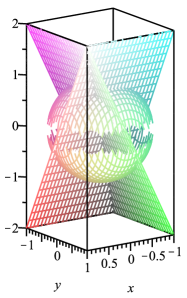
Figure 14: Sets $\mathcal{S}_{1}$ (143) and $\mathcal{R}_{2}$ (144). $\mathcal{R}_{2}$ is in the foreground underneath the $z=2x$ and $z=2y$ planes.

See 2.4

Proof.

In what follows, let

$$\mathcal{R}_{\rho} \coloneqq\left\{\left(x,y,z\right)^{\mathsf{T}}\in\mathbb{R}^{3}:\rho\max\left(x,y\right)\leq z\right\}$$ (143)

$$\mathcal{S}_{r} \coloneqq\left\{\left(x,y,z\right)^{\mathsf{T}}\in\mathbb{R}^{3}:x^{2}+y^{2}+z^{2}\leq r^{2}\right\}$$ (144)

so that $\mathcal{R}_{\rho}\subset\mathbb{R}^{3}$ gives an infinite wedge whose spine passes through the origin and $\mathcal{S}_{r}\subset\mathbb{R}^{3}$ gives the sphere with center $\mathbf{0}$ and radius $r>0$ (Figure 14). These in place, we note that $\mathrm{Var}\left(Z_{\rho,0}\right)=\mathbb{E}Z_{\rho,0}^{2}-\left(\mathbb{E}Z_{\rho,0}\right)^{2}=\mathbb{E}Z_{\rho,0}^{2}-\nicefrac{{1}}{{4}}$ (Corollary 2.2); i.e., we need only show that

$$\mathbb{E}Z_{\rho,0}^{2}=\frac{1}{2\pi}\cos^{-1}\left(-\frac{1}{\rho^{2}+1}\right)$$ (145)

To see this note that

$$\mathbb{E}Z_{\rho,0}^{2} =\rho\int_{0}^{1}y^{2}\frac{\phi\left(\rho\Phi^{-1}\left(y\right)\right)}{\phi\left(\Phi^{-1}\left(y\right)\right)}dy=\int_{-\infty}^{\infty}\Phi\left(\nicefrac{{z}}{{\rho}}\right)^{2}\phi\left(z\right)dz$$ (146)

$$=\int_{-\infty}^{\infty}\int_{-\infty}^{\nicefrac{{z}}{{\rho}}}\int_{-\infty}^{\nicefrac{{z}}{{\rho}}}\phi\left(x\right)\phi\left(y\right)\phi\left(z\right)dx\,dy\,dz=\Pr\left(\mathbf{Z}\in\mathcal{R}_{\rho}\right)$$ (147)

where $\mathbf{Z}\sim\mathcal{N}_{3}\left(\mathbf{0},\mathbf{I}_{3}\right)$ for $\mathbf{I}_{k}$ the $k\times k$ identity matrix. Now, since $\mathcal{N}_{3}\left(\mathbf{0},\mathbf{I}_{3}\right)$ is spherically-symmetric about $\mathbf{0}$, we have

$$\Pr\left(\mathbf{Z}\in\mathcal{R}_{\rho}\right) =\lim_{r\rightarrow\infty}\Pr\left(\mathbf{Z}\in\mathcal{R}_{\rho},\mathbf{Z}\in\mathcal{S}_{r}\right)$$ (148)

$$=\lim_{r\rightarrow\infty}\Pr\left(\left.\mathbf{Z}\in\mathcal{R}_{\rho}\right|\mathbf{Z}\in\mathcal{S}_{r}\right)\Pr\left(\mathbf{Z}\in\mathcal{S}_{r}\right)$$ (149)

$$=\lim_{r\rightarrow\infty}\frac{\mathrm{Volume}\left(\mathcal{R}_{\rho}\cap\mathcal{S}_{r}\right)}{\mathrm{Volume}\left(\mathcal{S}_{r}\right)}\Pr\left(\mathbf{Z}\in\mathcal{S}_{r}\right)$$ (150)

$$=\lim_{r\rightarrow\infty}\frac{\left(\nicefrac{{\theta_{\rho}}}{{2\pi}}\right)\mathrm{Volume}\left(\mathcal{S}_{r}\right)}{\mathrm{Volume}\left(\mathcal{S}_{r}\right)}\Pr\left(\mathbf{Z}\in\mathcal{S}_{r}\right)=\frac{\theta_{\rho}}{2\pi}$$ (151)

where (151) comes from the observation that $\mathcal{R}_{\rho}\cap\mathcal{S}_{r}$ is a spherical wedge with volume $\left(\nicefrac{{\theta_{\rho}}}{{2\pi}}\right)\mathrm{Volume}\left(\mathcal{S}_{r}\right)$ for $\theta_{\rho}$ the angle swept out by the wedge. To see that

$$\theta_{\rho}=\cos^{-1}\left(-\frac{1}{\rho^{2}+1}\right)$$ (152)

note that $\left\{\alpha\left(1,1,\rho\right)^{\mathsf{T}}\right\}_{\alpha\in\mathbb{R}}$ gives the spine of $\mathcal{R}_{\rho}$ (Figure 14). With $\mathbf{s}\coloneqq\left(1,1,\rho\right)^{\mathsf{T}}$,

• $\mathbf{a}\coloneqq\left(-1,1+\rho^{2},-\rho\right)^{\mathsf{T}}$ is on the $z=\rho x$ side of the wedge and $\mathbf{a}^{\mathsf{T}}\mathbf{s}=0$;

• $\mathbf{b}\coloneqq\left(1+\rho^{2},-1,-\rho\right)^{\mathsf{T}}$ is on the $z=\rho y$ side of the wedge and $\mathbf{b}^{\mathsf{T}}\mathbf{s}=0$.

With $\mathbf{a}$ and $\mathbf{b}$ on either side of the wedge, both orthogonal to $\mathbf{s}$, we have

$$\theta_{\rho}=\cos^{-1}\left(\frac{\mathbf{a}^{\mathsf{T}}\mathbf{b}}{\left\|\mathbf{a}\right\|\left\|\mathbf{b}\right\|}\right)=\cos^{-1}\left(-\frac{1}{\rho^{2}+1}\right)$$ (153)

which, together with (145), (147), and (151), gives the desired result. ∎

Appendix B Proofs for Section 2.1.2

See 2.5

Proof.

Note that

$$f_{\rho,-\delta}\left(y\right) =\frac{\rho\phi\left(-\delta+\rho\Phi^{-1}\left(y\right)\right)}{\phi\left(\Phi^{-1}\left(y\right)\right)}=\frac{\rho\phi\left(-\delta-\rho\Phi^{-1}\left(1-y\right)\right)}{\phi\left(-\Phi^{-1}\left(1-y\right)\right)}$$ (154)

$$=\frac{\rho\phi\left(\delta+\rho\Phi^{-1}\left(1-y\right)\right)}{\phi\left(\Phi^{-1}\left(1-y\right)\right)}=f_{\rho,\delta}\left(1-y\right)$$ (155)

where (154) uses the odd symmetry of $\Phi$ about the $x=0,y=\nicefrac{{1}}{{2}}$ axes and (155) uses the even symmetry of $\phi$ about $x=0$. ∎

See 2.6

Proof.

We first note that

$$\mathbb{E}Z_{\rho,-\delta} =\int_{0}^{1}yf_{\rho,-\delta}\left(y\right)dy=\int_{0}^{1}yf_{\rho,\delta}\left(1-y\right)dy$$ (156)

$$=\int_{0}^{1}\left(1-x\right)f_{\rho,\delta}\left(x\right)dx=1-\mathbb{E}Z_{\rho,\delta}$$ (157)

where (156) uses Theorem 2.5. Using this result, we next note that

$$\mathrm{Var}\left(Z_{\rho,-\delta}\right) =\int_{0}^{1}\left(y-\mathbb{E}Z_{\rho,-\delta}\right)^{2}f_{\rho,-\delta}\left(y\right)dy$$ (158)

$$=\int_{0}^{1}\left(y-\left(1-\mathbb{E}Z_{\rho,\delta}\right)\right)^{2}f_{\rho,\delta}\left(1-y\right)dy$$ (159)

$$=\int_{0}^{1}\left(\left(1-x\right)-\left(1-\mathbb{E}Z_{\rho,\delta}\right)\right)^{2}f_{\rho,\delta}\left(x\right)dx$$ (160)

$$=\int_{0}^{1}\left(x-\mathbb{E}Z_{\rho,\delta}\right)^{2}f_{\rho,\delta}\left(x\right)dx=\mathrm{Var}\left(Z_{\rho,\delta}\right)$$ (161)

where (159) uses Theorem 2.5 and $\mathbb{E}Z_{\rho,-\delta}=1-\mathbb{E}Z_{\rho,\delta}$. ∎

See 2.8

Proof.

Using (7) and independent $X_{0}\sim\mathcal{N}\left(0,1\right)$ and $X_{1}\sim\mathcal{N}\left(\delta,\rho^{2}\right)$ (see footnote 3), we first note that

$$\mathbb{E}Z_{\rho,\delta} =\int_{0}^{1}z\frac{\rho\phi\left(\delta+\rho\Phi^{-1}\left(z\right)\right)}{\phi\left(\Phi^{-1}\left(z\right)\right)}dz=\int_{-\infty}^{\infty}\Phi\left(\frac{y-\delta}{\rho}\right)\phi\left(y\right)dy$$ (162)

$$=\mathbb{E}\left[\Pr\left(\left.X_{1}\leq X_{0}\right|X_{0}\right)\right]=\Pr\left(X_{1}\leq X_{0}\right)$$ (163)

In what follows let $\mathcal{R}\coloneqq\left\{\left(x,y\right)^{\mathsf{T}}\in\mathbb{R}^{2}:x>y\right\}$. Note that

$$\mathbb{E}Z_{\rho,\delta} =\int_{0}^{1}\left(1-\Phi\left(\delta+\rho\Phi^{-1}\left(z\right)\right)\right)dz$$ (164)

$$=1-\int_{-\infty}^{\infty}\Phi\left(x\right)\frac{1}{\rho}\phi\left(\frac{x-\delta}{\rho}\right)dx$$ (165)

$$=1-\int_{-\infty}^{\infty}\int_{-\infty}^{x}f\left(x\right)\phi\left(y\right)dy\,dx$$ (166)

where $f\left(x\right)\coloneqq\frac{1}{\rho}\phi\left(\frac{x-\delta}{\rho}\right)$ is the density function for $\mathcal{N}\left(\delta,\rho^{2}\right)$. This implies that

$$\mathbb{E}Z_{\rho,\delta}=1-\Pr\left(\mathbf{X}\in\mathcal{R}\right)=\Pr\left(\mathbf{X}\in\mathcal{R}^{\mathsf{c}}\right)$$ (167)

where $\mathcal{R}^{\mathsf{c}}\coloneqq\left\{\left(x,y\right)^{\mathsf{T}}\in\mathbb{R}^{2}:x\leq y\right\}$ and

$$\mathbf{X}\sim\mathcal{N}_{2}\left(\left(\begin{array}[]{c}\delta\\ 0\end{array}\right),\left(\begin{array}[]{cc}\rho^{2}&0\\ 0&1\end{array}\right)\right)$$ (168)

Transforming $\mathbb{R}^{2}$ makes probability (167) easier to calculate. To that end, while

$$\mathbf{R}\coloneqq\left[\begin{array}[]{rr}\cos\left(\frac{\pi}{4}\right)&-\sin\left(\frac{\pi}{4}\right)\\ \sin\left(\frac{\pi}{4}\right)&\cos\left(\frac{\pi}{4}\right)\end{array}\right]=\frac{1}{\sqrt{2}}\left[\begin{array}[]{rr}1&-1\\ 1&1\end{array}\right]$$ (169)

rotates $\mathbb{R}^{2}$ counterclockwise by $\frac{\pi}{4}\textrm{ radians}=45^{\circ}$, we have

$$\mathbf{R}\mathcal{R}^{c} \coloneqq\left\{\mathbf{R}\mathbf{x}:\mathbf{x}\in\mathcal{R}^{c}\right\}=\left\{\left(x,y\right)^{\mathsf{T}}\in\mathbb{R}^{2}:x\leq 0\right\}$$ (170)

$$\mathbf{Y} \coloneqq\mathbf{R}\mathbf{X}\sim\mathcal{N}_{2}\left(\frac{\delta}{\sqrt{2}}\left(\begin{array}[]{c}1\\ 1\end{array}\right),\frac{1}{2}\left(\begin{array}[]{cc}\rho^{2}+1&\rho^{2}-1\\ \rho^{2}-1&\rho^{2}+1\end{array}\right)\right)$$ (175)

Equations (170) and (175) then imply that

$$\mathbb{E}Z_{\rho,\delta} =\Pr\left(\mathbf{X}\in\mathcal{R}^{\mathsf{c}}\right)=\Pr\left(\mathbf{R}\mathbf{X}\in\mathbf{R}\mathcal{R}^{\mathsf{c}}\right)$$ (176)

$$=\Pr\left(Y_{1}\leq 0\right)=\Phi\left(\nicefrac{{-\delta}}{{\sqrt{1+\rho^{2}}}}\right)$$ (177)

where (176) uses (167) and (177) uses the marginal $Y_{1}\sim\mathcal{N}\left(\frac{\delta}{\sqrt{2}},\frac{1+\rho^{2}}{2}\right)$. ∎

See 2.10

Proof.

With $\Phi\left(\nicefrac{{\delta}}{{\sqrt{\rho^{2}+1}}}\right)=1-\mathbb{E}Z_{\rho,\delta}$ and $\mathrm{Var}\left(Z_{\rho,\delta}\right)=\mathbb{E}Z_{\rho,\delta}^{2}-\left(\mathbb{E}Z_{\rho,\delta}\right)^{2}$, we have

$$\Phi\left(\nicefrac{{-\delta}}{{\sqrt{\rho^{2}+1}}}\right)\Phi\left(\nicefrac{{\delta}}{{\sqrt{\rho^{2}+1}}}\right)-\mathrm{Var}\left(Z_{\rho,\delta}\right)=\mathbb{E}\left[Z_{\rho,\delta}\left(1-Z_{\rho,\delta}\right)\right]>0$$ (178)

because $\Pr\left(0<Z_{\rho,\delta}<1\right)=1$. For the other inequalities, note that $Z_{\rho,\delta}$ varies when $0<\rho,\left|\delta\right|<\infty$ and that $\Phi\left(\nicefrac{{-\delta}}{{\sqrt{\rho^{2}+1}}}\right)\Phi\left(\nicefrac{{\delta}}{{\sqrt{\rho^{2}+1}}}\right)\in\left(0,\nicefrac{{1}}{{4}}\right]$. ∎

See 2.11

Proof.

We prove each part in turn, noting first that

$$\frac{d}{dy}f_{\rho,\delta}\left(y\right) =\frac{\rho\phi\left(\delta+\rho\Phi^{-1}\left(y\right)\right)}{\phi\left(\Phi^{-1}\left(y\right)\right)^{2}}\left\{\left(1-\rho^{2}\right)\Phi^{-1}\left(y\right)-\rho\delta\right\}$$ (179)

The first term of (179) is positive; the second term can be positive or negative.

1. When $\rho>1$, (179) gives

   $$y\lesseqqgtr\Phi\left(\nicefrac{{-\rho\delta}}{{\left(\rho^{2}-1\right)}}\right)\iff\frac{d}{dy}f_{\rho,\delta}\left(y\right)\gtreqqless 0$$ (180)

   which implies the result.

2. When $\rho=0$ and $\delta=1$, we have CDF $\Phi\left(\Phi^{-1}\left(y\right)\right)=y$ for $y\in\left(0,1\right)$, and the result easily follows.

3. When $\rho<1$, (179) gives

   $$y\lesseqqgtr\Phi\left(\nicefrac{{-\rho\delta}}{{\left(\rho^{2}-1\right)}}\right)\iff\frac{d}{dy}f_{\rho,\delta}\left(y\right)\lesseqqgtr 0$$ (181)

   so that $\arg\max_{y}f_{\rho,\delta}\left(y\right)=\left\{0,1\right\}$. Now,

   $$\lim_{y\rightarrow 0^{+}}f_{\rho,\delta}\left(y\right)=\lim_{y\rightarrow 0^{+}}\rho e^{\frac{1-\rho^{2}}{2}\Phi^{-1}\left(y\right)^{2}-\rho\delta\Phi^{-1}\left(y\right)-\frac{\delta^{2}}{2}}=\infty$$ (182)

   because the $\Phi^{-1}\left(y\right)^{2}$ term dominates the exponent and $0<\rho<1$ implies that $\nicefrac{{\left(1-\rho^{2}\right)}}{{2}}>0$. The same argument gives $\lim_{y\rightarrow 1^{-}}f_{\rho,\delta}\left(y\right)=\infty$.

4. When $\rho=1$ and $\delta>0$, (179) gives $\frac{d}{dy}f_{\rho,\delta}\left(y\right)<0$, so that $\arg\max_{y}f_{1,\delta}\left(y\right)=0$. We further note that

   $$\lim_{y\rightarrow 0^{+}}f_{1,\delta}\left(y\right)=\lim_{y\rightarrow 0^{+}}\rho\exp\left(-\frac{\delta\left(\delta+2\Phi^{-1}\left(y\right)\right)}{2}\right)=\infty$$ (183)

5. When $\rho=1$ and $\delta<0$, (179) gives $\frac{d}{dy}f_{\rho,\delta}\left(y\right)>0$, so that $\arg\max_{y}f_{1,\delta}\left(y\right)=1$. We further note that

   $$\lim_{y\rightarrow 1^{-}}f_{1,\delta}\left(y\right)=\lim_{y\rightarrow 1^{-}}\rho\exp\left(-\frac{\delta\left(\delta+2\Phi^{-1}\left(y\right)\right)}{2}\right)=\infty$$ (184)

∎

See 2.13

Proof.

In what follows let $\mathcal{R}\coloneqq\left\{\left(x,y,z\right)^{\mathsf{T}}\in\mathbb{R}^{3}:\max\left(x,y\right)\leq z\right\}$. By Theorem 2.8 it suffices to show that

$$\mathbb{E}Z_{\rho,\delta}^{2}=\int_{\nicefrac{{11\pi}}{{12}}}^{\nicefrac{{19\pi}}{{12}}}G_{\rho,\delta}\left(\theta\right)d\theta+\frac{\cos^{-1}\left(\nicefrac{{-1}}{{\left(\rho^{2}+1\right)}}\right)}{2\pi\exp\left(\nicefrac{{\delta^{2}}}{{\left(\rho^{2}+2\right)}}\right)}$$ (185)

To that end, with independent $X_{0}\sim\mathcal{N}\left(0,1\right)$, $X_{1},X_{2}\sim\mathcal{N}\left(\delta,\rho^{2}\right)$ (see footnote 3), note first that,

$$\mathbb{E}Z_{\rho,\delta}^{2} =\rho\int_{0}^{1}y^{2}\frac{\phi\left(\delta+\rho\Phi^{-1}\left(y\right)\right)}{\phi\left(\Phi^{-1}\left(y\right)\right)}dy=\int_{-\infty}^{\infty}\Phi\left(\frac{z-\delta}{\rho}\right)^{2}\phi\left(z\right)dz$$ (186)

$$=\mathbb{E}\left[\Pr\left(\left.X_{1}\leq X_{0},X_{2}\leq X_{0}\right|X_{0}\right)\right]=\Pr\left(X_{1}\leq X_{0},X_{2}\leq X_{0}\right)$$ (187)

$$=\int_{-\infty}^{\infty}\int_{-\infty}^{z}\int_{-\infty}^{z}f\left(x\right)f\left(y\right)\phi\left(z\right)dx\,dy\,dz$$ (188)

where $f\left(x\right)\coloneqq\frac{1}{\rho}\phi\left(\frac{x-\delta}{\rho}\right)$ is the density function for $\mathcal{N}\left(\delta,\rho^{2}\right)$. This implies that

$$\mathbb{E}Z_{\rho,\delta}^{2}=\Pr\left(\mathbf{X}\in\mathcal{R}\right)$$ (189)

where

$$\mathbf{X}\sim\mathcal{N}_{3}\left(\left[\begin{array}[]{c}\delta\\ \delta\\ 0\end{array}\right],\left[\begin{array}[]{ccc}\rho^{2}&0&0\\ 0&\rho^{2}&0\\ 0&0&1\end{array}\right]\right)$$ (190)

Transforming $\mathbb{R}^{3}$ makes probability (189) easier to calculate. Namely, we rotate the space so that the spine $\alpha\left(1,1,1\right)^{\mathsf{T}}$, $\alpha\in\mathbb{R}$, of wedge $\mathcal{R}$ is vertical, thereby shrinking the problem from three dimensions to two (see Figure 14). Letting $\mathbf{s}\coloneqq\left(1,1,1\right)^{\mathsf{T}}$ and $\mathbf{v}\coloneqq\left(0,0,1\right)^{\mathsf{T}}$, we rotate $\mathbb{R}^{3}$ by

$$\cos^{-1}\left(\frac{\mathbf{s}^{\mathsf{T}}\mathbf{v}}{\left\|\mathbf{s}\right\|\left\|\mathbf{v}\right\|}\right)=\cos^{-1}\left(\frac{1}{\sqrt{3}}\right)\textrm{ radians}$$ (191)

about unit axis $\mathbf{u}\coloneqq\left(\nicefrac{{1}}{{\sqrt{2}}},\nicefrac{{-1}}{{\sqrt{2}}},0\right)^{\mathsf{T}}$ using rotation matrix

$$\mathbf{R}\coloneqq\frac{1}{6}\left[\begin{array}[]{rrr}\sqrt{3}+3&\sqrt{3}-3&-2\sqrt{3}\\ \sqrt{3}-3&\sqrt{3}+3&-2\sqrt{3}\\ 2\sqrt{3}&2\sqrt{3}&2\sqrt{3}\end{array}\right]$$ (192)

(see Equation 9.63 in Cole (2015)). We then have

$$\mathbf{Y}\coloneqq\mathbf{R}\mathbf{X}\sim\mathcal{N}_{3}\left(\frac{1}{\sqrt{3}}\left[\begin{array}[]{r}\delta\\ \delta\\ 2\delta\end{array}\right],\frac{1}{3}\left[\begin{array}[]{rrr}1+2\rho^{2}&1-\rho^{2}&-1+\rho^{2}\\ 1-\rho^{2}&1+2\rho^{2}&-1+\rho^{2}\\ -1+\rho^{2}&-1+\rho^{2}&1+2\rho^{2}\end{array}\right]\right)$$ (193)

Furthermore, with

$$\left[\begin{array}[]{c}a\\ b\\ c\end{array}\right]\coloneqq\mathbf{R}\left[\begin{array}[]{r}1\\ 0\\ 0\end{array}\right]=\frac{1}{6}\left[\begin{array}[]{r}3+\sqrt{3}\\ -3+\sqrt{3}\\ 2\sqrt{3}\end{array}\right]\textrm{ and }\mathbf{R}\left[\begin{array}[]{r}0\\ 1\\ 0\end{array}\right]=\left[\begin{array}[]{c}b\\ a\\ c\end{array}\right]$$ (194)

we note that

$$\mathbf{R}\mathcal{R} =\left\{\left(x,y,z\right)^{\mathsf{T}}\in\mathbb{R}^{3}:y\leq\min\left(\frac{ax}{b},\frac{bx}{a}\right)\right\}$$ (195)

$$=\left\{\left(r,\theta,z\right)^{\mathsf{T}}\in\left[0,\infty\right)\times\left[0,2\pi\right)\times\mathbb{R}:\frac{11\pi}{12}\leq\theta\leq\frac{19\pi}{12}\right\}$$ (196)

where the product $\mathbf{R}\mathcal{R}$ is defined in (170) and (196) uses polar coordinates for the $xy$-plane. Now, (195) implies we need only consider $\left(Y_{1},Y_{2}\right)^{\mathsf{T}}$ which has marginal distribution

$$\left[\begin{array}[]{r}Y_{1}\\ Y_{2}\end{array}\right]\sim\mathcal{N}_{2}\left(\frac{1}{\sqrt{3}}\left[\begin{array}[]{c}\delta\\ \delta\end{array}\right],\frac{1}{3}\left[\begin{array}[]{rr}1+2\rho^{2}&1-\rho^{2}\\ 1-\rho^{2}&1+2\rho^{2}\end{array}\right]\right)\eqqcolon\mathcal{N}_{2}\left(\boldsymbol{\mu},\boldsymbol{\Sigma}\right)$$ (197)

and density function

$$g\left(\mathbf{y}\right)\coloneqq\frac{\exp\left(-\frac{1}{2}\left(\mathbf{y}-\boldsymbol{\mu}\right)^{\mathsf{T}}\boldsymbol{\Sigma}^{-1}\left(\mathbf{y}-\boldsymbol{\mu}\right)\right)}{2\pi\sqrt{\left|\boldsymbol{\Sigma}\right|}}$$ (198)

where $\left|\boldsymbol{\Sigma}\right|=\frac{1}{3}\rho^{2}\left(\rho^{2}+2\right)$ is the determinant of $\boldsymbol{\Sigma}$ and $\mathbf{y}\in\mathbb{R}^{2}$. Picking up from (189), we have $\mathbb{E}Z_{\rho,\delta}^{2}=\Pr\left(\mathbf{X}\in\mathcal{R}\right)=\Pr\left(\mathbf{R}\mathbf{X}\in\mathbf{R}\mathcal{R}\right)$

$$=\Pr\left(Y_{2}\leq\min\left(\frac{aY_{1}}{b},\frac{bY_{1}}{a}\right)\right)$$ (199)

$$=\underset{y_{2}\leq\min\left(\frac{ay_{1}}{b},\frac{by_{1}}{a}\right)}{\int\int}g\left(\mathbf{y}\right)dy_{1}dy_{2}$$ (200)

$$=\int_{\nicefrac{{11\pi}}{{12}}}^{\nicefrac{{19\pi}}{{12}}}\int_{0}^{\infty}g\left(r\cos\theta,r\sin\theta\right)r\,dr\,d\theta$$ (201)

$$=\frac{\sqrt{3}e^{-\frac{\delta^{2}}{\rho^{2}+2}}}{2\pi\rho\sqrt{\rho^{2}+2}}\int_{\nicefrac{{11\pi}}{{12}}}^{\nicefrac{{19\pi}}{{12}}}\int_{0}^{\infty}\exp\left(B_{\rho,\delta}\left(\theta\right)r-A_{\rho}\left(\theta\right)r^{2}\right)r\,dr\,d\theta$$ (202)

$$=\frac{\sqrt{3}e^{-\frac{\delta^{2}}{\rho^{2}+2}}}{2\pi\rho\sqrt{\rho^{2}+2}}\int_{\nicefrac{{11\pi}}{{12}}}^{\nicefrac{{19\pi}}{{12}}}\frac{1}{2A_{\rho}\left(\theta\right)}\left[\frac{B_{\rho,\delta}\left(\theta\right)}{\sqrt{2A_{\rho}\left(\theta\right)}}\frac{\Phi\left(\frac{B_{\rho,\delta}\left(\theta\right)}{\sqrt{2A_{\rho}\left(\theta\right)}}\right)}{\phi\left(\frac{B_{\rho,\delta}\left(\theta\right)}{\sqrt{2A_{\rho}\left(\theta\right)}}\right)}+1\right]d\theta$$ (203)

with $B_{\rho,\delta}\left(\theta\right)$ and $A_{\rho}\left(\theta\right)>0$ as in (18) and (19). We finally have $\int_{\nicefrac{{11\pi}}{{12}}}^{\nicefrac{{19\pi}}{{12}}}\frac{d\theta}{2A_{\rho}\left(\theta\right)}$

$$=\int_{\nicefrac{{11\pi}}{{12}}}^{\nicefrac{{19\pi}}{{12}}}\frac{\rho^{2}\left(\rho^{2}+2\right)d\theta}{\rho^{2}\left(\sin\left(2\theta\right)+2\right)+2\cos^{2}\left(\theta+\nicefrac{{\pi}}{{4}}\right)}$$ (204)

$$=\rho\sqrt{\frac{\rho^{2}+2}{3}}\left[\pi-\tan^{-1}\left(\frac{\left(2+\sqrt{3}\right)\rho^{2}+\sqrt{3}+1}{\rho\sqrt{\rho^{2}+2}}\right)\right.$$ (205)

$$\hphantom{aaaaaaaaaaaaaaaaaaaaaaaaa}\left.-\tan^{-1}\left(\frac{\left(2-\sqrt{3}\right)\rho^{2}-\sqrt{3}+1}{\rho\sqrt{\rho^{2}+2}}\right)\right]$$ (206)

$$=\rho\sqrt{\frac{\rho^{2}+2}{3}}\left[\pi-\tan^{-1}\left(\rho\sqrt{\rho^{2}+2}\right)\right]=\rho\sqrt{\frac{\rho^{2}+2}{3}}\cos^{-1}\left(-\frac{1}{\rho^{2}+1}\right)$$ (207)

where the first part of (207) uses the identity $\tan^{-1}u+\tan^{-1}v=\tan^{-1}\frac{u+v}{1-uv}\mod\pi$, when $uv\neq 1$, and the second part uses basic trigonometry. Substituting (207) into (203) gives (22) and (185)–(187) gives (21), completing the proof. ∎

Lemma B.1.

The function $G_{\rho,\delta}$ in Theorem 2.13 is symmetric in $\theta$ about $\nicefrac{{5\pi}}{{4}}$.

Proof.

With $\theta\in\mathbb{R}$ it is enough to show that $f_{i}\left(\theta+\nicefrac{{5\pi}}{{4}}\right)=f_{i}\left(\nicefrac{{5\pi}}{{4}}-\theta\right)$ for

$$f_{1}\left(\theta\right) \coloneqq\sin\left(\theta+\nicefrac{{\pi}}{{4}}\right)$$ (208)

$$f_{2}\left(\theta\right) \coloneqq\cos^{2}\left(\theta+\nicefrac{{\pi}}{{4}}\right)$$ (209)

$$f_{3}\left(\theta\right) \coloneqq\sin\left(2\theta\right)$$ (210)

because functions $G_{\rho,\delta}$ depends on $\theta$ through these. To that end, note that

$$f_{1}\left(\theta+\nicefrac{{5\pi}}{{4}}\right) =\sin\left(\theta+\nicefrac{{3\pi}}{{2}}\right)$$ (211)

$$=\sin\left(\pi-\nicefrac{{3\pi}}{{2}}-\theta\right)$$ (212)

$$=\sin\left(\nicefrac{{-\pi}}{{2}}-\theta+2\pi\right)$$ (213)

$$=\sin\left(\nicefrac{{5\pi}}{{4}}-\theta+\nicefrac{{\pi}}{{4}}\right)=f_{1}\left(\nicefrac{{5\pi}}{{4}}-\theta\right)$$ (214)

$$f_{2}\left(\theta+\nicefrac{{5\pi}}{{4}}\right) =\cos^{2}\left(\theta+\nicefrac{{3\pi}}{{2}}\right)$$ (215)

$$=\cos^{2}\left(\pi-\nicefrac{{3\pi}}{{2}}-\theta\right)$$ (216)

$$=\cos^{2}\left(\nicefrac{{-\pi}}{{2}}-\theta+2\pi\right)$$ (217)

$$=\cos^{2}\left(\nicefrac{{5\pi}}{{4}}-\theta+\nicefrac{{\pi}}{{4}}\right)=f_{2}\left(\nicefrac{{5\pi}}{{4}}-\theta\right)$$ (218)

$$f_{3}\left(\theta+\nicefrac{{5\pi}}{{4}}\right) =\sin\left(\nicefrac{{5\pi}}{{2}}+2\theta\right)$$ (219)

$$=\sin\left(\pi-\nicefrac{{5\pi}}{{2}}-2\theta\right)$$ (220)

$$=\sin\left(\nicefrac{{-3\pi}}{{2}}-2\theta+4\pi\right)$$ (221)

$$=\sin\left(2\left(\nicefrac{{5\pi}}{{4}}-\theta\right)\right)=f_{3}\left(\nicefrac{{5\pi}}{{4}}-\theta\right)$$ (222)

∎

The following technical lemma helps us prove Proposition 2.23 (via Proposition B.3) and Theorem 3.6 (via Lemma E.1).

Lemma B.2.

Let

$$H_{\rho,\delta}\left(\theta\right) \coloneqq\frac{\sqrt{3}e^{-\frac{\delta^{2}}{\rho^{2}+2}}}{2\pi\rho\sqrt{\rho^{2}+2}}\frac{B_{\rho,\delta}\left(\theta\right)}{\left[2A_{\rho}\left(\theta\right)\right]^{\nicefrac{{3}}{{2}}}}\frac{1}{\phi\left(\frac{B_{\rho,\delta}\left(\theta\right)}{\sqrt{2A_{\rho}\left(\theta\right)}}\right)}$$ (223)

$$=G_{\rho,\delta}\left(\theta\right)\left/\Phi\left(\frac{B_{\rho,\delta}\left(\theta\right)}{\sqrt{2A_{\rho}\left(\theta\right)}}\right)\right.$$ (224)

with $B_{\rho,\delta}\left(\theta\right)$, $A_{\rho}\left(\theta\right)$, and $G_{\rho,\delta}\left(\theta\right)$ as in (18), (19), and (20). Then,

$$\int_{\nicefrac{{11\pi}}{{12}}}^{\nicefrac{{19\pi}}{{12}}}H_{\rho,\delta}\left(\theta\right)d\theta=1-2\Phi\left(\nicefrac{{\delta}}{{\sqrt{\rho^{2}+1}}}\right)$$ (225)

Proof.

Letting

$$\tau_{1}\left(\delta\right)\coloneqq\int_{\nicefrac{{11\pi}}{{12}}}^{\nicefrac{{19\pi}}{{12}}}G_{\rho,\delta}\left(\theta\right)d\theta$$ (226)

$$\tau_{2}\left(\delta\right)\coloneqq\frac{\cos^{-1}\left(\nicefrac{{-1}}{{\left(\rho^{2}+1\right)}}\right)}{2\pi\exp\left(\nicefrac{{\delta^{2}}}{{\left(\rho^{2}+2\right)}}\right)},\quad\tau_{3}\left(\delta\right)\coloneqq\Phi\left(\nicefrac{{-\delta}}{{\sqrt{\rho^{2}+1}}}\right)^{2}$$ (227)

we have $\tau_{1}\left(\delta\right)+\tau_{2}\left(\delta\right)-\tau_{3}\left(\delta\right)=\tau_{1}\left(-\delta\right)+\tau_{2}\left(-\delta\right)-\tau_{3}\left(-\delta\right)$ by Corollary 2.6 and Theorem 2.13. Now,

$$\tau_{1}\left(-\delta\right) =\int_{\nicefrac{{11\pi}}{{12}}}^{\nicefrac{{19\pi}}{{12}}}G_{\rho,-\delta}\left(\theta\right)d\theta$$ (228)

$$=\frac{\sqrt{3}e^{-\frac{\delta^{2}}{\rho^{2}+2}}}{2\pi\rho\sqrt{\rho^{2}+2}}\int_{\nicefrac{{11\pi}}{{12}}}^{\nicefrac{{19\pi}}{{12}}}\frac{B_{\rho,-\delta}\left(\theta\right)}{\left[2A_{\rho}\left(\theta\right)\right]^{\nicefrac{{3}}{{2}}}}\frac{\Phi\left(\frac{B_{\rho,-\delta}\left(\theta\right)}{\sqrt{2A_{\rho}\left(\theta\right)}}\right)}{\phi\left(\frac{B_{\rho,-\delta}\left(\theta\right)}{\sqrt{2A_{\rho}\left(\theta\right)}}\right)}d\theta$$ (229)

$$=-\frac{\sqrt{3}e^{-\frac{\delta^{2}}{\rho^{2}+2}}}{2\pi\rho\sqrt{\rho^{2}+2}}\int_{\nicefrac{{11\pi}}{{12}}}^{\nicefrac{{19\pi}}{{12}}}\frac{B_{\rho,\delta}\left(\theta\right)}{\left[2A_{\rho}\left(\theta\right)\right]^{\nicefrac{{3}}{{2}}}}\frac{\Phi\left(-\frac{B_{\rho,\delta}\left(\theta\right)}{\sqrt{2A_{\rho}\left(\theta\right)}}\right)}{\phi\left(-\frac{B_{\rho,\delta}\left(\theta\right)}{\sqrt{2A_{\rho}\left(\theta\right)}}\right)}d\theta$$ (230)

$$=-\frac{\sqrt{3}e^{-\frac{\delta^{2}}{\rho^{2}+2}}}{2\pi\rho\sqrt{\rho^{2}+2}}\int_{\nicefrac{{11\pi}}{{12}}}^{\nicefrac{{19\pi}}{{12}}}\frac{B_{\rho,\delta}\left(\theta\right)}{\left[2A_{\rho}\left(\theta\right)\right]^{\nicefrac{{3}}{{2}}}}\frac{\left[1-\Phi\left(\frac{B_{\rho,\delta}\left(\theta\right)}{\sqrt{2A_{\rho}\left(\theta\right)}}\right)\right]}{\phi\left(\frac{B_{\rho,\delta}\left(\theta\right)}{\sqrt{2A_{\rho}\left(\theta\right)}}\right)}d\theta$$ (231)

$$=\int_{\nicefrac{{11\pi}}{{12}}}^{\nicefrac{{19\pi}}{{12}}}G_{\rho,\delta}\left(\theta\right)d\theta-\int_{\nicefrac{{11\pi}}{{12}}}^{\nicefrac{{19\pi}}{{12}}}H_{\rho,\delta}\left(\theta\right)d\theta$$ (232)

$$=\tau_{1}\left(\delta\right)-\int_{\nicefrac{{11\pi}}{{12}}}^{\nicefrac{{19\pi}}{{12}}}H_{\rho,\delta}\left(\theta\right)d\theta$$ (233)

because $B_{\rho,-\delta}\left(\theta\right)=-B_{\rho,\delta}\left(\theta\right)$. Note that $\tau_{2}\left(-\delta\right)=\tau_{2}\left(\delta\right)$. We finally have

$$\tau_{3}\left(-\delta\right) =\Phi\left(\nicefrac{{\delta}}{{\sqrt{\rho^{2}+1}}}\right)^{2}$$ (234)

$$=\left[1-\Phi\left(\nicefrac{{-\delta}}{{\sqrt{\rho^{2}+1}}}\right)\right]^{2}$$ (235)

$$=1-2\Phi\left(\nicefrac{{-\delta}}{{\sqrt{\rho^{2}+1}}}\right)+\Phi\left(\nicefrac{{-\delta}}{{\sqrt{\rho^{2}+1}}}\right)^{2}$$ (236)

$$=1-2\Phi\left(\nicefrac{{-\delta}}{{\sqrt{\rho^{2}+1}}}\right)+\tau_{3}\left(\delta\right)$$ (237)

$$=-1+2\Phi\left(\nicefrac{{\delta}}{{\sqrt{\rho^{2}+1}}}\right)+\tau_{3}\left(\delta\right)$$ (238)

Putting this all together with $\tau_{1}\left(\delta\right)+\tau_{2}\left(\delta\right)-\tau_{3}\left(\delta\right)=\tau_{1}\left(-\delta\right)+\tau_{2}\left(-\delta\right)-\tau_{3}\left(-\delta\right)$ gives the desired result. ∎

The following proposition bounds the integral in $\mathrm{Var}\left(Z_{\rho,\delta}\right)$ (Theorem 2.13).

Proposition B.3.

With $G_{\rho,\delta}\left(\theta\right)$ as in (20), we have

$$\int_{\nicefrac{{11\pi}}{{12}}}^{\nicefrac{{19\pi}}{{12}}}G_{\rho,\delta}\left(\theta\right)d\theta\leq\Phi\left(\nicefrac{{-\sqrt{2}\delta}}{{\sqrt{\rho^{2}+2}}}\right)\left[1-2\Phi\left(\nicefrac{{\delta}}{{\sqrt{\rho^{2}+1}}}\right)\right]$$ (239)

Proof.

The proof relies on Lemma B.2. We first consider the case $\delta>0$. Note first that $G_{\rho,\delta}\left(\theta\right)<0$ for $\delta>0$ and $\nicefrac{{11\pi}}{{12}}<\theta<\nicefrac{{19\pi}}{{12}}$. This follows from the definitions of $B_{\rho,\delta}\left(\theta\right)$ and $G_{\rho,\delta}\left(\theta\right)$ in (18) and (20), namely $\sin\left(\theta+\nicefrac{{\pi}}{{4}}\right)<0$ for $\nicefrac{{11\pi}}{{12}}<\theta<\nicefrac{{19\pi}}{{12}}$. This implies that

$$\int_{\nicefrac{{11\pi}}{{12}}}^{\nicefrac{{19\pi}}{{12}}}G_{\rho,\delta}\left(\theta\right)d\theta \leq\int_{\nicefrac{{11\pi}}{{12}}}^{\nicefrac{{19\pi}}{{12}}}H_{\rho,\delta}\left(\theta\right)d\theta\min_{\frac{11\pi}{12}\leq\theta\leq\frac{19\pi}{12}}\Phi\left(\nicefrac{{B_{\rho,\delta}\left(\theta\right)}}{{\sqrt{2A_{\rho}\left(\theta\right)}}}\right)$$ (240)

$$=\left[1-2\Phi\left(\nicefrac{{\delta}}{{\sqrt{\rho^{2}+1}}}\right)\right]\Phi\left(\nicefrac{{B_{\rho,\delta}\left(\frac{5\pi}{4}\right)}}{{\sqrt{2A_{\rho}\left(\frac{5\pi}{4}\right)}}}\right)$$ (241)

$$=\left[1-2\Phi\left(\nicefrac{{\delta}}{{\sqrt{\rho^{2}+1}}}\right)\right]\Phi\left(\nicefrac{{-\sqrt{2}\delta}}{{\sqrt{\rho^{2}+2}}}\right)$$ (242)

where (241) uses Lemma B.2.

We now turn to the case $\delta<0$. Note that $B_{\rho,\delta}\left(\theta\right)>0$ when $\delta<0$ and $\nicefrac{{11\pi}}{{12}}\leq\theta\leq\nicefrac{{19\pi}}{{12}}$ implies that $G_{\rho,\delta}\left(\theta\right)>0$ when $\delta<0$ and $\nicefrac{{11\pi}}{{12}}\leq\theta\leq\nicefrac{{19\pi}}{{12}}$. Following a path similar to that above, we have

$$\int_{\nicefrac{{11\pi}}{{12}}}^{\nicefrac{{19\pi}}{{12}}}G_{\rho,\delta}\left(\theta\right)d\theta \leq\int_{\nicefrac{{11\pi}}{{12}}}^{\nicefrac{{19\pi}}{{12}}}H_{\rho,\delta}\left(\theta\right)d\theta\max_{\frac{11\pi}{12}\leq\theta\leq\frac{19\pi}{12}}\Phi\left(\nicefrac{{B_{\rho,\delta}\left(\theta\right)}}{{\sqrt{2A_{\rho}\left(\theta\right)}}}\right)$$ (243)

$$=\left[1-2\Phi\left(\nicefrac{{\delta}}{{\sqrt{\rho^{2}+1}}}\right)\right]\Phi\left(\nicefrac{{B_{\rho,\delta}\left(\frac{5\pi}{4}\right)}}{{\sqrt{2A_{\rho}\left(\frac{5\pi}{4}\right)}}}\right)$$ (244)

$$=\left[1-2\Phi\left(\nicefrac{{\delta}}{{\sqrt{\rho^{2}+1}}}\right)\right]\Phi\left(\nicefrac{{-\sqrt{2}\delta}}{{\sqrt{\rho^{2}+2}}}\right)$$ (245)

where (244) uses Lemma B.2. We finally note that $G_{\rho,0}\left(\theta\right)=1-2\Phi\left(\nicefrac{{0}}{{\sqrt{\rho^{2}+1}}}\right)=0$, so that the bound works when $\delta=0$. This completes the proof. ∎

One can similarly show that

$$\left[1-2\Phi\left(\nicefrac{{\delta}}{{\sqrt{\rho^{2}+1}}}\right)\right]\Phi\left(\nicefrac{{-\rho\delta}}{{\sqrt{\left(\rho^{2}+1\right)\left(\rho^{2}+2\right)}}}\right)\leq\int_{\nicefrac{{11\pi}}{{12}}}^{\nicefrac{{19\pi}}{{12}}}G_{\rho,\delta}\left(\theta\right)d\theta$$ (246)

Panels (239) and (246) imply upper and lower bounds for $\mathrm{Var}\left(Z_{\rho,\delta}\right)$. The upper bound $v_{\uparrow}\left(\rho,\delta\right)$ approximates the variance. Only for $\delta\approx 0$ is the lower bound $v_{\downarrow}\left(\rho,\delta\right)$ positive. $\mathrm{Var}\left(Z_{\rho,\delta}\right)$ and $v_{\uparrow}\left(\rho,\delta\right)$ approach zero from above while $v_{\downarrow}\left(\rho,\delta\right)$ approaches zero from below as $\left|\delta\right|\rightarrow\infty$ (cf. Proposition 2.10).

See 2.15

Proof.

We first show this for $0\leq\delta_{1}<\delta_{2}$, so that $\Phi\left(\nicefrac{{-\left(\delta_{1}+\delta_{2}\right)}}{{2\rho}}\right)<\nicefrac{{1}}{{2}}$. In this setting the result follows if we can show that

$$f_{\rho,\delta_{1}}\left(z\right)\lesseqqgtr f_{\rho,\delta_{2}}\left(z\right)\textrm{ when }z\lesseqqgtr\Phi\left(-\frac{\delta_{1}+\delta_{2}}{2\rho}\right)$$ (247)

so that $f_{\rho,\delta_{2}}$ is more concentrated than $f_{\rho,\delta_{1}}$. Arguing (247), we have:

$$z\lesseqqgtr\Phi\left(-\frac{\delta_{1}+\delta_{2}}{2\rho}\right) \iff\Phi^{-1}\left(z\right)\lesseqqgtr-\frac{\delta_{1}+\delta_{2}}{2\rho}$$ (248)

$$\iff\Phi^{-1}\left(z\right)\lesseqqgtr-\frac{\delta_{2}^{2}-\delta_{1}^{2}}{2\rho\left(\delta_{2}-\delta_{1}\right)}$$ (249)

$$\iff 2\rho\delta_{1}\Phi^{-1}\left(z\right)+\delta_{1}^{2}\gtreqqless 2\rho\delta_{2}\Phi^{-1}\left(z\right)+\delta_{2}^{2}$$ (250)

$$\iff f_{\rho,\delta_{1}}\left(z\right)\lesseqqgtr f_{\rho,\delta_{2}}\left(z\right)$$ (251)

where (251) uses

$$f_{\rho,\delta}\left(z\right)=\rho\exp\left\{-\nicefrac{{1}}{{2}}\left[\left(\rho^{2}-1\right)\Phi^{-1}\left(z\right)^{2}+2\rho\delta\Phi^{-1}\left(z\right)+\delta^{2}\right]\right\}$$ (252)

Corollary 2.6 gives $\mathrm{Var}\left(Z_{\rho,\pm\delta}\right)=\mathrm{Var}\left(Z_{\rho,\left|\delta\right|}\right)$, thereby completing the proof. ∎

Appendix C Proofs for Section 2.2

See 2.16

Proof.

Both claims follow from Chebyshev’s inequality. Fixing $\epsilon>0$ and $\delta$ large enough, we have

$$\Pr\left(\left|Z_{\rho,\delta}\right|>\epsilon\right) =\Pr\left(\left|Z_{\rho,\delta}-\Phi\left(\nicefrac{{-\delta}}{{\sqrt{\rho^{2}+1}}}\right)+\Phi\left(\nicefrac{{-\delta}}{{\sqrt{\rho^{2}+1}}}\right)\right|>\epsilon\right)$$ (253)

$$\leq\Pr\left(\left|Z_{\rho,\delta}-\Phi\left(\nicefrac{{-\delta}}{{\sqrt{\rho^{2}+1}}}\right)\right|>\epsilon-\Phi\left(\nicefrac{{-\delta}}{{\sqrt{\rho^{2}+1}}}\right)\right)$$ (254)

$$\leq\mathrm{Var}\left(Z_{\rho,\delta}\right)\left/\left(\epsilon-\Phi\left(\nicefrac{{-\delta}}{{\sqrt{\rho^{2}+1}}}\right)\right)^{2}\right.\stackrel{{\scriptstyle[}}{{\infty}}]{\delta}{\longrightarrow}0$$ (255)

where (254) uses the triangle inequality and (255) uses Chebyshev’s inequality, Theorem 2.8, and Proposition 2.10. This proves that $Z_{\rho,\delta}\longrightarrow 0$ in probability as $\delta\rightarrow\infty$. To prove the second claim we fix $\epsilon>0$ and $\delta$ small enough. We then use the same argument to obtain

$$\Pr\left(\left|Z_{\rho,\delta}-1\right|>\epsilon\right)\leq\frac{\mathrm{Var}\left(Z_{\rho,\delta}\right)}{\left(\epsilon-\left|\Phi\left(\nicefrac{{-\delta}}{{\sqrt{\rho^{2}+1}}}\right)-1\right|\right)^{2}}\stackrel{{\scriptstyle[}}{{-}}\infty]{\delta}{\longrightarrow}0$$ (256)

which proves that $Z_{\rho,\delta}\longrightarrow 1$ in probability as $\delta\rightarrow-\infty$. ∎

See 2.17

Proof.

For $\epsilon\in\left(0,1\right)$ it is enough to show that

$$\lim_{\epsilon\rightarrow 0^{+}}\lim_{\rho\rightarrow 0^{+}}\Pr\left(Z_{\rho,\delta}\leq\epsilon\right) =\Phi\left(\delta\right)$$ (257)

$$\lim_{\epsilon\rightarrow 1^{-}}\lim_{\rho\rightarrow 0^{+}}\Pr\left(Z_{\rho,\delta}\geq\epsilon\right) =\Phi\left(-\delta\right)$$ (258)

To that end note that

$$\lim_{\epsilon\rightarrow 0^{+}}\lim_{\rho\rightarrow 0^{+}}\Pr\left(Z_{\rho,\delta}\leq\epsilon\right) =\lim_{\epsilon\rightarrow 0^{+}}\lim_{\rho\rightarrow 0^{+}}\Phi\left(\delta+\rho\Phi^{-1}\left(\epsilon\right)\right)$$ (259)

$$=\lim_{\epsilon\rightarrow 0^{+}}\Phi\left(\delta\right)=\Phi\left(\delta\right)$$ (260)

and that

$$\lim_{\epsilon\rightarrow 1^{-}}\lim_{\rho\rightarrow 0^{+}}\Pr\left(Z_{\rho,\delta}\geq\epsilon\right) =\lim_{\epsilon\rightarrow 1^{-}}\lim_{\rho\rightarrow 0^{+}}\Pr\left(Z_{\rho,\delta}>\epsilon\right)$$ (261)

$$=\lim_{\epsilon\rightarrow 1^{-}}\lim_{\rho\rightarrow 0^{+}}\left\{1-\Phi\left(\delta+\rho\Phi^{-1}\left(\epsilon\right)\right)\right\}$$ (262)

$$=\lim_{\epsilon\rightarrow 1^{-}}\left\{1-\Phi\left(\delta\right)\right\}=\Phi\left(-\delta\right)$$ (263)

where (261) uses the continuity of $Z_{\rho,\delta}$, and (260) and (263) use $\left|\Phi^{-1}\left(\epsilon\right)\right|<\infty$ for $\epsilon\in\left(0,1\right)$ and the continuity of $\Phi$. This completes the proof. ∎

See 2.18

Proof.

Expanding $\Phi^{-1}\left(x\right)$ about $\Phi\left(\nicefrac{{-\delta}}{{\sqrt{\rho^{2}+1}}}\right)$ we have

$$\Phi^{-1}\left(x\right) =\Phi^{-1}\left(\Phi\left(\nicefrac{{-\delta}}{{\sqrt{\rho^{2}+1}}}\right)\right)+\frac{x-\Phi\left(\nicefrac{{-\delta}}{{\sqrt{\rho^{2}+1}}}\right)}{\phi\left(\Phi^{-1}\left(x^{*}\right)\right)}$$ (264)

$$=-\frac{\delta}{\sqrt{\rho^{2}+1}}+\frac{x-\Phi\left(\nicefrac{{-\delta}}{{\sqrt{\rho^{2}+1}}}\right)}{\phi\left(\Phi^{-1}\left(x^{*}\right)\right)}$$ (265)

where $x^{*}$ is between $x$ and $\Phi\left(\nicefrac{{-\delta}}{{\sqrt{\rho^{2}+1}}}\right)$. Now, fixing $y\in\mathbb{R}$, we have

$$\Pr\left(\rho\left(Z_{\rho,\delta}-\Phi\left(\nicefrac{{-\delta}}{{\sqrt{\rho^{2}+1}}}\right)\right)\leq y\right) =\Pr\left(Z_{\rho,\delta}\leq\Phi\left(\nicefrac{{-\delta}}{{\sqrt{\rho^{2}+1}}}\right)+\nicefrac{{y}}{{\rho}}\right)$$ (266)

$$=\Phi\left(\delta+\rho\Phi^{-1}\left(\Phi\left(\nicefrac{{-\delta}}{{\sqrt{\rho^{2}+1}}}\right)+\nicefrac{{y}}{{\rho}}\right)\right)$$ (267)

$$=\Phi\left(\delta\left(1-\nicefrac{{\rho}}{{\sqrt{\rho^{2}+1}}}\right)+\nicefrac{{y}}{{\phi\left(\Phi^{-1}\left(y^{*}\right)\right)}}\right)$$ (268)

$$\stackrel{{\scriptstyle\rho\rightarrow\infty}}{{\longrightarrow}}\Phi\left(\sqrt{2\pi}y\right)$$ (269)

where (268) uses (265) with $y^{*}$ between $\Phi\left(\nicefrac{{-\delta}}{{\sqrt{\rho^{2}+1}}}\right)+\nicefrac{{y}}{{\rho}}$ and $\Phi\left(\nicefrac{{-\delta}}{{\sqrt{\rho^{2}+1}}}\right)$ and (269) follows because $y^{*}\rightarrow\nicefrac{{1}}{{2}}$ as $\rho\rightarrow\infty$. This completes the proof. ∎

See 2.19

Proof.

First, we note that Proposition 2.18 implies that

$$\lim_{\rho\rightarrow\infty}2\pi\rho^{2}\mathrm{Var}\left(Z_{\rho,\delta}\right)=1$$ (270)

Then, fixing $\epsilon>0$ and $\rho$ sufficiently large, we have $\Pr\left(\left|Z_{\rho,\delta}-\nicefrac{{1}}{{2}}\right|>\epsilon\right)$

$$\leq\Pr\left(\left|Z_{\rho,\delta}-\Phi\left(\nicefrac{{-\delta}}{{\sqrt{\rho^{2}+1}}}\right)\right|>\epsilon-\left|\nicefrac{{1}}{{2}}-\Phi\left(\nicefrac{{-\delta}}{{\sqrt{\rho^{2}+1}}}\right)\right|\right)$$ (271)

$$\leq\mathrm{Var}\left(Z_{\rho,\delta}\right)\left/\left(\epsilon-\left|\nicefrac{{1}}{{2}}-\Phi\left(\nicefrac{{-\delta}}{{\sqrt{\rho^{2}+1}}}\right)\right|\right)^{2}\right.\stackrel{{\scriptstyle[}}{{\infty}}]{\rho}{\longrightarrow}0$$ (272)

where (271) uses the triangle inequality and (272) uses Chebyshev’s inequality and (270). This completes the proof. ∎

See 2.20

Proof.

Expanding $\Phi^{-1}\left(x\right)$ about $\Phi\left(\nicefrac{{-\delta}}{{\sqrt{\rho^{2}+1}}}\right)$ we have

$$\Phi^{-1}\left(x\right) =\Phi^{-1}\left(\Phi\left(\nicefrac{{-\delta}}{{\sqrt{\rho^{2}+1}}}\right)\right)+\frac{x-\Phi\left(\nicefrac{{-\delta}}{{\sqrt{\rho^{2}+1}}}\right)}{\phi\left(\Phi^{-1}\left(x^{*}\right)\right)}$$ (273)

$$=-\frac{\delta}{\sqrt{\rho^{2}+1}}+\frac{x-\Phi\left(\nicefrac{{-\delta}}{{\sqrt{\rho^{2}+1}}}\right)}{\phi\left(\Phi^{-1}\left(x^{*}\right)\right)}$$ (274)

where $x^{*}$ is between $x$ and $\Phi\left(\nicefrac{{-\delta}}{{\sqrt{\rho^{2}+1}}}\right)$. Now, fixing $y\in\mathbb{R}$, we have

$$\Pr\left(\rho\left(Z_{\rho,\delta}-\Phi\left(\nicefrac{{-\delta}}{{\sqrt{\rho^{2}+1}}}\right)\right)\leq y\right) =\Pr\left(Z_{\rho,\delta}\leq\Phi\left(\nicefrac{{-\delta}}{{\sqrt{\rho^{2}+1}}}\right)+\nicefrac{{y}}{{\rho}}\right)$$ (275)

$$=\Phi\left(\delta+\rho\Phi^{-1}\left(\Phi\left(\nicefrac{{-\delta}}{{\sqrt{\rho^{2}+1}}}\right)+\nicefrac{{y}}{{\rho}}\right)\right)$$ (276)

$$=\Phi\left(\delta\left(1-\nicefrac{{\rho}}{{\sqrt{\rho^{2}+1}}}\right)+\nicefrac{{y}}{{\phi\left(\Phi^{-1}\left(y^{*}\right)\right)}}\right)$$ (277)

$$=\Phi\left(r\left(\rho-\nicefrac{{\rho^{2}}}{{\sqrt{\rho^{2}+1}}}\right)+\nicefrac{{y}}{{\phi\left(\Phi^{-1}\left(y^{*}\right)\right)}}\right)$$ (278)

$$\stackrel{{\scriptstyle\rho,\left|\delta\right|\rightarrow\infty}}{{\longrightarrow}}\Phi\left(\nicefrac{{y}}{{\phi\left(-r\right)}}\right)=\Phi\left(\nicefrac{{y}}{{\phi\left(r\right)}}\right)$$ (279)

where (277) uses (274) with $y^{*}$ between $\Phi\left(\nicefrac{{-\delta}}{{\sqrt{\rho^{2}+1}}}\right)+\nicefrac{{y}}{{\rho}}$ and $\Phi\left(\nicefrac{{-\delta}}{{\sqrt{\rho^{2}+1}}}\right)$ and (279) follows because $y^{*}$ approaches $\Phi\left(-r\right)$ as $\rho,\left|\delta\right|\rightarrow\infty$ and $\nicefrac{{\delta}}{{\rho}}=r$ remains fixed. This completes the proof. ∎

See 2.21

Proof.

First, we note that Proposition 2.20 implies that

$$\lim_{\rho,\left|\delta\right|\rightarrow\infty}\left.\rho^{2}\mathrm{Var}\left(Z_{\rho,\delta}\right)\right/\phi\left(r\right)^{2}=1$$ (280)

for $r=\nicefrac{{\delta}}{{\rho}}$ fixed. With $\epsilon>0$ and $\rho,\left|\delta\right|$ large enough, $\Pr\left(\left|Z_{\rho,\delta}-\Phi\left(-r\right)\right|>\epsilon\right)$

$$\leq\Pr\left(\left|Z_{\rho,\delta}-\Phi\left(\nicefrac{{-\delta}}{{\sqrt{\rho^{2}+1}}}\right)\right|>\epsilon-\left|\Phi\left(\nicefrac{{-\delta}}{{\sqrt{\rho^{2}+1}}}\right)-\Phi\left(-r\right)\right|\right)$$ (281)

$$\leq\mathrm{Var}\left(Z_{\rho,\delta}\right)\left/\left(\epsilon-\left|\Phi\left(\nicefrac{{-\delta}}{{\sqrt{\rho^{2}+1}}}\right)-\Phi\left(-r\right)\right|\right)^{2}\right.\stackrel{{\scriptstyle\rho,\left|\delta\right|\rightarrow\infty}}{{\longrightarrow}}0$$ (282)

where (281) uses the triangle inequality, (282) uses Chebyshev’s inequality, and the limit uses (280) and keeps $r=\nicefrac{{\delta}}{{\rho}}$ fixed. This completes the proof. ∎

Appendix D Proofs for Section 2.4

See 2.22

Proof.

We prove the first claim. The second follows in a similar way. First, we note that

$$\hat{\lim}\,\mathrm{Var}\left(X_{\alpha,\beta}\right) =\hat{\lim}\,\frac{\alpha\beta}{\left(\alpha+\beta\right)^{2}\left(\alpha+\beta+1\right)}$$ (283)

$$=\hat{\lim}\,\frac{\alpha}{\left(\alpha+\beta\right)^{2}\left(1+\nicefrac{{\alpha}}{{\beta}}+\nicefrac{{1}}{{\beta}}\right)}=0$$ (284)

where $\hat{\lim}$ is the limit where $\beta\rightarrow\infty$ and $\alpha=o\left(\beta\right)$. Now, fix $\epsilon>0$ and $\beta$ large enough. Then,

$$\hat{\lim}\,\Pr\left(\left|X_{\alpha,\beta}\right|>\epsilon\right) \leq\hat{\lim}\,\Pr\left(\left|X_{\alpha,\beta}-\nicefrac{{\alpha}}{{\left(\alpha+\beta\right)}}\right|>\epsilon-\nicefrac{{\alpha}}{{\left(\alpha+\beta\right)}}\right)$$ (285)

$$\leq\hat{\lim}\,\left.\mathrm{Var}\left(X_{\alpha,\beta}\right)\right/\left(\epsilon-\nicefrac{{\alpha}}{{\left(\alpha+\beta\right)}}\right)^{2}=0$$ (286)

where (285) follows from the triangle inequality and (286) follows from Chebyshev’s inequality and (284). This completes the proof. ∎

See 2.23

Proof.

Note first that

$$\mathbb{E}X_{\alpha_{3},\beta_{3}}=\frac{\alpha_{3}}{\alpha_{3}+\beta_{3}}=\Phi\left(\nicefrac{{-\delta}}{{\sqrt{\rho^{2}+1}}}\right)\rightarrow\left\{\begin{array}[]{rl}0&\textrm{ as }\delta\rightarrow\infty\\ 1&\textrm{ as }\delta\rightarrow-\infty\end{array}\right.$$ (287)

We will show that

$$\begin{array}[]{rcl}\beta_{3}\left(\rho,\delta\right)=&\frac{\Phi\left(\nicefrac{{-\delta}}{{\sqrt{\rho^{2}+1}}}\right)\Phi\left(\nicefrac{{\delta}}{{\sqrt{\rho^{2}+1}}}\right)^{2}}{\mathrm{Var}\left(Z_{\rho,\delta}\right)}-\Phi\left(\nicefrac{{\delta}}{{\sqrt{\rho^{2}+1}}}\right)&\stackrel{{\scriptstyle[}}{{\infty}}]{\delta}{\longrightarrow}\infty\\ \alpha_{3}\left(\rho,\delta\right)=&\frac{\Phi\left(\nicefrac{{-\delta}}{{\sqrt{\rho^{2}+1}}}\right)^{2}\Phi\left(\nicefrac{{\delta}}{{\sqrt{\rho^{2}+1}}}\right)}{\mathrm{Var}\left(Z_{\rho,\delta}\right)}-\Phi\left(\nicefrac{{-\delta}}{{\sqrt{\rho^{2}+1}}}\right)&\stackrel{{\scriptstyle[}}{{-}}\infty]{\delta}{\longrightarrow}\infty\end{array}$$ (288)

which, together with (287), implies that $\alpha_{3}=o\left(\beta_{3}\right)$ as $\delta\rightarrow\infty$ and $\beta_{3}=o\left(\alpha_{3}\right)$ as $\delta\rightarrow-\infty$. In our efforts to prove (288) we start by noting that, by symmetry (see Corollary 2.6), we need only show one of these. We prove the first. To that end, note that

$$\lim_{\delta\rightarrow\infty}\beta_{3}\left(\rho,\delta\right) =\lim_{\delta\rightarrow\infty}\left\{\frac{\Phi\left(\nicefrac{{-\delta}}{{\sqrt{\rho^{2}+1}}}\right)\Phi\left(\nicefrac{{\delta}}{{\sqrt{\rho^{2}+1}}}\right)^{2}}{\mathrm{Var}\left(Z_{\rho,\delta}\right)}-\Phi\left(\nicefrac{{\delta}}{{\sqrt{\rho^{2}+1}}}\right)\right\}$$ (289)

$$=\lim_{\delta\rightarrow\infty}\frac{\Phi\left(\nicefrac{{-\delta}}{{\sqrt{\rho^{2}+1}}}\right)}{\mathrm{Var}\left(Z_{\rho,\delta}\right)}-1$$ (290)

where (290) uses $\lim_{\delta\rightarrow\infty}\Phi\left(\nicefrac{{\delta}}{{\sqrt{\rho^{2}+1}}}\right)=1$. If we can show that

$$\lim_{\delta\rightarrow\infty}\left(\frac{\Phi\left(\nicefrac{{-\delta}}{{\sqrt{\rho^{2}+1}}}\right)}{\mathrm{Var}\left(Z_{\rho,\delta}\right)}\right)^{-1}=\lim_{\delta\rightarrow\infty}\frac{\mathrm{Var}\left(Z_{\rho,\delta}\right)}{\Phi\left(\nicefrac{{-\delta}}{{\sqrt{\rho^{2}+1}}}\right)}=0$$ (291)

we have the desired result. Note then that

$$\frac{\mathrm{Var}\left(Z_{\rho,\delta}\right)}{\Phi\left(\nicefrac{{-\delta}}{{\sqrt{\rho^{2}+1}}}\right)}\leq\frac{\cos^{-1}\left(\nicefrac{{-1}}{{\left(\rho^{2}+1\right)}}\right)}{2\pi\exp\left(\nicefrac{{\delta^{2}}}{{\left(\rho^{2}+2\right)}}\right)\Phi\left(\nicefrac{{-\delta}}{{\sqrt{\rho^{2}+1}}}\right)}-\frac{\Phi\left(\nicefrac{{-\sqrt{2}\delta}}{{\sqrt{\rho^{2}+2}}}\right)}{\Phi\left(\nicefrac{{-\delta}}{{\sqrt{\rho^{2}+1}}}\right)}$$ (292)

where (292) uses Theorem 2.13, Proposition B.3, $\lim_{\delta\rightarrow\infty}\Phi\left(\nicefrac{{\delta}}{{\sqrt{\rho^{2}+1}}}\right)=1$, and $\lim_{\delta\rightarrow\infty}\Phi\left(\nicefrac{{-\delta}}{{\sqrt{\rho^{2}+1}}}\right)=0$. We then have

$$\lim_{\delta\rightarrow\infty}\frac{\Phi\left(\nicefrac{{-\delta}}{{\sqrt{\rho^{2}+1}}}\right)}{\exp\left(\nicefrac{{-\delta^{2}}}{{\left(\rho^{2}+2\right)}}\right)} =\lim_{\delta\rightarrow\infty}\frac{\left(\rho^{2}+2\right)\exp\left(\nicefrac{{\rho^{2}\delta^{2}}}{{2\left(\rho^{2}+1\right)\left(\rho^{2}+2\right)}}\right)}{2\delta\sqrt{2\pi\left(\rho^{2}+1\right)}}$$ (293)

$$=\infty$$ (294)

$$\lim_{\delta\rightarrow\infty}\frac{\Phi\left(\nicefrac{{-\sqrt{2}\delta}}{{\sqrt{\rho^{2}+2}}}\right)}{\Phi\left(\nicefrac{{-\delta}}{{\sqrt{\rho^{2}+1}}}\right)} =\sqrt{\frac{2\left(\rho^{2}+1\right)}{\rho^{2}+2}}\lim_{\delta\rightarrow\infty}\exp\left(-\frac{\rho^{2}\delta^{2}}{2\left(\rho^{2}+1\right)\left(\rho^{2}+2\right)}\right)$$ (295)

$$=0$$ (296)

where (293) and (295) use L’Hôpital’s rule. Using (294) and (296) in (292) gives (291). Substituting (291) into (290) gives $\lim_{\delta\rightarrow\infty}\beta_{3}\left(\rho,\delta\right)=\infty$, which proves (288). This together with Lemma 2.22 proves (46).

Summarizing (46) and Proposition 2.16 we have the following convergence in probability

$$X_{\alpha_{3}\left(\rho,\delta\right),\beta_{3}\left(\rho,\delta\right)} \stackrel{{\scriptstyle[}}{{\infty}}]{\delta}{\longrightarrow}0\textrm{ and }Z_{\rho,\delta}\stackrel{{\scriptstyle[}}{{\infty}}]{\delta}{\longrightarrow}0$$ (297)

$$X_{\alpha_{3}\left(\rho,\delta\right),\beta_{3}\left(\rho,\delta\right)} \stackrel{{\scriptstyle[}}{{-}}\infty]{\delta}{\longrightarrow}1\textrm{ and }Z_{\rho,\delta}\stackrel{{\scriptstyle[}}{{-}}\infty]{\delta}{\longrightarrow}1$$ (298)

Letting $Y_{c}\equiv c\in\mathbb{R}$, we have

$$0\leq W_{2}\left(Z_{\rho,\delta},X_{\alpha_{3},\beta_{3}}\right)\leq W_{2}\left(Z_{\rho,\delta},Y_{c}\right)+W_{2}\left(X_{\alpha_{3},\beta_{3}},Y_{c}\right)$$

by the triangle inequality for the 2-Wasserstein metric (Clement & Desch (2008)), so that

$$\lim_{\delta\rightarrow\infty}W_{2}\left(Z_{\rho,\delta},Y_{0}\right) =\lim_{\delta\rightarrow\infty}W_{2}\left(X_{\alpha_{3},\beta_{3}},Y_{0}\right)=0$$ (299)

$$\lim_{\delta\rightarrow-\infty}W_{2}\left(Z_{\rho,\delta},Y_{1}\right) =\lim_{\delta\rightarrow-\infty}W_{2}\left(X_{\alpha_{3},\beta_{3}},Y_{1}\right)=0$$ (300)

implies that $\lim_{\left|\delta\right|\rightarrow\infty}W_{2}\left(Z_{\rho,\delta},X_{\alpha_{3},\beta_{3}}\right)=0$. The 2-Wasserstein distance between two random variables goes to zero iff they converge in distribution and their second moments converge (Panaretos & Zemel (2019)). The above convergence in probability implies convergence in distribution (Grimmett & Stirzaker (2001) Theorem 7.2.3). Further, Proposition 2.10, the above argument, and the proof of Lemma 2.22 give

$$\lim_{\delta\rightarrow\infty}\mathbb{E}Z_{\rho,\delta}^{2} =\lim_{\delta\rightarrow\infty}\mathbb{E}X_{\alpha_{3},\beta_{3}}^{2}=\mathbb{E}Y_{0}^{2}=0$$ (301)

$$\lim_{\delta\rightarrow-\infty}\mathbb{E}Z_{\rho,\delta}^{2} =\lim_{\delta\rightarrow-\infty}\mathbb{E}X_{\alpha_{3},\beta_{3}}^{2}=\mathbb{E}Y_{1}^{2}=1$$ (302)

because $\lim_{\left|\delta\right|\rightarrow\infty}\mathrm{Var}\left(Z_{\rho,\delta}\right)=0$ and $\lim_{\left|\delta\right|\rightarrow\infty}\mathrm{Var}\left(X_{\alpha_{3},\beta_{3}}\right)=0$ imply that

$$\lim_{\left|\delta\right|\rightarrow\infty}\mathbb{E}Z_{\rho,\delta}^{2} =\lim_{\left|\delta\right|\rightarrow\infty}\mathbb{E}\left[Z_{\rho,\delta}\right]^{2}$$ (303)

$$\lim_{\left|\delta\right|\rightarrow\infty}\mathbb{E}X_{\alpha_{3},\beta_{3}}^{2} =\lim_{\left|\delta\right|\rightarrow\infty}\mathbb{E}\left[X_{\alpha_{3},\beta_{3}}\right]^{2}$$ (304)

That is to say, we have both convergence in distribution and of second moments, which completes the proof. ∎

See 2.24

Proof.

Let $B\left(x;\alpha,\beta\right)\coloneqq\int_{0}^{x}y^{\alpha-1}\left(1-y\right)^{\beta-1}dy$ be the incomplete beta function. The key observation is that $B\left(x;\alpha,\beta\right)=\alpha^{-1}x^{\alpha}\left(1+\mathcal{O}\left(x\right)\right)$ as $x\rightarrow 0^{+}$ (Pearson (1968)). We also note that $\Gamma\left(x\right)\sim\nicefrac{{1}}{{x}}-\gamma$, for Euler’s constant $\gamma\approx 0.577216$, as $x\rightarrow 0^{+}$. Then, for $\epsilon\in\left(0,1\right)$, we have

$$\Pr\left(X_{\alpha,\beta}\leq\epsilon\right) =\frac{B\left(\epsilon;\alpha,\beta\right)}{B\left(\alpha,\beta\right)}=\frac{B\left(\epsilon;\alpha,\beta\right)\Gamma\left(\alpha+\beta\right)}{\Gamma\left(\alpha\right)\Gamma\left(\beta\right)}$$ (305)

$$\sim\frac{\beta\epsilon^{\alpha}}{\alpha+\beta}\frac{1-\left(\alpha+\beta\right)\gamma}{\left(1-\alpha\gamma\right)\left(1-\beta\gamma\right)}\rightarrow 1-\lambda$$ (306)

where $\sim$ assumes $\alpha,\beta,\epsilon$ small and $\rightarrow$ sends $\alpha,\beta,\epsilon$ to zero from above. That is to say, we have $\lim_{\alpha,\beta,\epsilon\rightarrow 0^{+}}\Pr\left(X_{\alpha,\beta}\leq\epsilon\right)=1-\lambda$. Noting that $B\left(x;\alpha,\beta\right)=B\left(\alpha,\beta\right)-B\left(1-x;\beta,\alpha\right)$, we next have

$$\Pr\left(X_{\alpha,\beta}\geq 1-\epsilon\right) =1-\frac{B\left(1-\epsilon;\alpha,\beta\right)}{B\left(\alpha,\beta\right)}=\frac{B\left(\epsilon;\beta,\alpha\right)\Gamma\left(\alpha+\beta\right)}{\Gamma\left(\alpha\right)\Gamma\left(\beta\right)}$$ (307)

$$\sim\frac{\alpha\epsilon^{\beta}}{\alpha+\beta}\frac{1-\left(\alpha+\beta\right)\gamma}{\left(1-\alpha\gamma\right)\left(1-\beta\gamma\right)}\rightarrow\lambda$$ (308)

where $\sim$ assumes $\alpha,\beta,\epsilon$ small and $\rightarrow$ sends $\alpha,\beta,\epsilon$ to zero from above. That is to say, we have $\lim_{\alpha,\beta,\epsilon\rightarrow 0^{+}}\Pr\left(X_{\alpha,\beta}\geq 1-\epsilon\right)=\lambda$, which completes the proof. ∎

See 2.25

Proof.

The convergence in distribution follows from Lemma 2.24 because

$$\lim_{\rho\rightarrow 0^{+}}\alpha_{3}\left(\rho,\delta\right) =\lim_{\rho\rightarrow 0^{+}}\Phi\left(\nicefrac{{-\delta}}{{\sqrt{\rho^{2}+1}}}\right)\left[\frac{\Phi\left(\nicefrac{{-\delta}}{{\sqrt{\rho^{2}+1}}}\right)\Phi\left(\nicefrac{{\delta}}{{\sqrt{\rho^{2}+1}}}\right)}{\mathrm{Var}\left(Z_{\rho,\delta}\right)}-1\right]$$ (309)

$$=\Phi\left(-\delta\right)\left[\frac{\Phi\left(-\delta\right)\Phi\left(\delta\right)}{\Phi\left(-\delta\right)\Phi\left(\delta\right)}-1\right]=0$$ (310)

$$\lim_{\rho\rightarrow 0^{+}}\beta_{3}\left(\rho,\delta\right) =\lim_{\rho\rightarrow 0^{+}}\Phi\left(\nicefrac{{\delta}}{{\sqrt{\rho^{2}+1}}}\right)\left[\frac{\Phi\left(\nicefrac{{-\delta}}{{\sqrt{\rho^{2}+1}}}\right)\Phi\left(\nicefrac{{\delta}}{{\sqrt{\rho^{2}+1}}}\right)}{\mathrm{Var}\left(Z_{\rho,\delta}\right)}-1\right]$$ (311)

$$=\Phi\left(\delta\right)\left[\frac{\Phi\left(-\delta\right)\Phi\left(\delta\right)}{\Phi\left(-\delta\right)\Phi\left(\delta\right)}-1\right]=0$$ (312)

and $\lim_{\rho\rightarrow 0^{+}}\nicefrac{{\alpha_{3}}}{{\left(\alpha_{3}+\beta_{3}\right)}}=\lim_{\rho\rightarrow 0^{+}}\Phi\left(\nicefrac{{-\delta}}{{\sqrt{\rho^{2}+1}}}\right)=\Phi\left(-\delta\right)\in\left(0,1\right)$, where (310) and (312) use Proposition 2.17. For $Y\sim\mathrm{Bernoulli}\left(\Phi\left(-\delta\right)\right)$, we then have

$$0\leq W_{2}\left(Z_{\rho,\delta},X_{\alpha_{3},\beta_{3}}\right)\leq W_{2}\left(Z_{\rho,\delta},Y\right)+W_{2}\left(X_{\alpha_{3},\beta_{3}},Y\right)$$ (313)

by the triangle inequality for the 2-Wasserstein metric (Clement & Desch (2008)), so that

$$\lim_{\rho\rightarrow 0^{+}}W_{2}\left(Z_{\rho,\delta},Y\right)=\lim_{\rho\rightarrow 0^{+}}W_{2}\left(X_{\alpha_{3},\beta_{3}},Y\right)=0$$ (314)

implies that $\lim_{\rho\rightarrow 0^{+}}W_{2}\left(Z_{\rho,\delta},X_{\alpha_{3},\beta_{3}}\right)=0$. The 2-Wasserstein distance between two random variables goes to zero iff they converge in distribution and their second moments converge (Panaretos & Zemel (2019)). Proposition 2.17 and the above argument show convergence in distribution. Proposition 2.17 and the above argument also give $\lim_{\rho\rightarrow 0^{+}}\mathbb{E}Z_{\rho,\delta}^{2}=\lim_{\rho\rightarrow 0^{+}}\mathbb{E}X_{\alpha_{3},\beta_{3}}^{2}=\mathbb{E}Y^{2}=\Phi\left(-\delta\right)$, completing the proof. ∎

See 2.26

Proof.

Without loss of generality we assume that $\alpha,\beta\in\left\{1,2,\ldots\right\}$. With $\xi_{i}\stackrel{{\scriptstyle\mathrm{iid}}}{{\sim}}\mathrm{Exp}\left(1\right)$, $1\leq i\leq\alpha+\beta$, let

$$G\coloneqq\sum_{i=1}^{\alpha}\xi_{i}\sim\mathrm{Gamma}\left(\alpha,1\right)\textrm{ and }G^{\prime}\coloneqq\sum_{i=\alpha+1}^{\alpha+\beta}\xi_{i}\sim\mathrm{Gamma}\left(\beta,1\right)$$ (315)

so that $G$ and $G^{\prime}$ are independent, and

$$X_{\alpha,\beta}\stackrel{{\scriptstyle\mathscr{L}}}{{=}}\frac{G}{G+G^{\prime}}\sim\mathrm{Beta}\left(\alpha,\beta\right)$$ (316)

Then,

$$\sqrt{\alpha+\beta}\left(X_{\alpha,\beta}-\frac{\alpha}{\alpha+\beta}\right) \stackrel{{\scriptstyle\mathscr{L}}}{{=}}\sqrt{\alpha+\beta}\left(\frac{\sum_{i=1}^{\alpha}\xi_{i}-\frac{\alpha}{\alpha+\beta}\sum_{i=1}^{\alpha+\beta}\xi_{i}}{\sum_{i=1}^{\alpha+\beta}\xi_{i}}\right)$$ (317)

$$=\frac{\frac{\sqrt{\alpha+\beta}}{\alpha+\beta}\frac{\beta}{\alpha+\beta}\sum_{i=1}^{\alpha}\xi_{i}-\frac{\sqrt{\alpha+\beta}}{\alpha+\beta}\frac{\alpha}{\alpha+\beta}\sum_{i=\alpha+1}^{\alpha+\beta}\xi_{i}}{\frac{1}{\alpha+\beta}\sum_{i=1}^{\alpha+\beta}\xi_{i}}$$ (318)

The first term in the numerator of (318) equals

$$\frac{\sqrt{\alpha+\beta}}{\alpha+\beta}\frac{\beta}{\alpha+\beta}\sum_{i=1}^{\alpha}\xi_{i} =\frac{1}{\sqrt{\alpha+\beta}}\frac{\beta}{\alpha+\beta}\left[\sum_{i=1}^{\alpha}\left(\xi_{i}-1\right)+\alpha\right]$$ (319)

$$=\sqrt{\frac{\alpha}{\alpha+\beta}}\frac{\beta}{\alpha+\beta}\frac{1}{\sqrt{\alpha}}\sum_{i=1}^{\alpha}\left(\xi_{i}-1\right)+\frac{\alpha\beta}{\left(\alpha+\beta\right)^{\nicefrac{{3}}{{2}}}}$$ (320)

The second term in the numerator of (318) equals

$$\frac{\sqrt{\alpha+\beta}}{\alpha+\beta}\frac{\alpha}{\alpha+\beta}\sum_{i=\alpha+1}^{\alpha+\beta}\xi_{i} =\frac{1}{\sqrt{\alpha+\beta}}\frac{\alpha}{\alpha+\beta}\left[\sum_{i=\alpha+1}^{\alpha+\beta}\left(\xi_{i}-1\right)+\beta\right]$$ (321)

$$=\sqrt{\frac{\beta}{\alpha+\beta}}\frac{\alpha}{\alpha+\beta}\frac{1}{\sqrt{\beta}}\sum_{i=\alpha+1}^{\alpha+\beta}\left(\xi_{i}-1\right)+\frac{\alpha\beta}{\left(\alpha+\beta\right)^{\nicefrac{{3}}{{2}}}}$$ (322)

Subtracting (322) from (320) we see that $\sqrt{\alpha+\beta}\left(X_{\alpha,\beta}-\frac{\alpha}{\alpha+\beta}\right)$ equals

$$\frac{\sqrt{\frac{\alpha}{\alpha+\beta}}\frac{\beta}{\alpha+\beta}\frac{1}{\sqrt{\alpha}}\sum_{i=1}^{\alpha}\left(\xi_{i}-1\right)-\sqrt{\frac{\beta}{\alpha+\beta}}\frac{\alpha}{\alpha+\beta}\frac{1}{\sqrt{\beta}}\sum_{i=\alpha+1}^{\alpha+\beta}\left(\xi_{i}-1\right)}{\frac{1}{\alpha+\beta}\sum_{i=1}^{\alpha+\beta}\xi_{i}}$$ (323)

To see that (323) converges to $\mathcal{N}\left(0,\lambda\left(1-\lambda\right)\right)$, note that

1. The denominator converges almost surely to one (SLLN);

2. $\sqrt{\frac{\alpha}{\alpha+\beta}}\frac{\beta}{\alpha+\beta}\frac{1}{\sqrt{\alpha}}\sum_{i=1}^{\alpha}\left(\xi_{i}-1\right)\stackrel{{\scriptstyle[}}{{\infty}}]{\alpha,\beta}{\Longrightarrow}\sqrt{\lambda}\left(1-\lambda\right)Z$, for $Z\sim\mathcal{N}\left(0,1\right)$ (CLT);

3. $\sqrt{\frac{\beta}{\alpha+\beta}}\frac{\alpha}{\alpha+\beta}\frac{1}{\sqrt{\beta}}\sum_{i=\alpha+1}^{\alpha+\beta}\left(\xi_{i}-1\right)\stackrel{{\scriptstyle[}}{{\infty}}]{\alpha,\beta}{\Longrightarrow}\lambda\sqrt{1-\lambda}Z^{\prime}$, for $Z^{\prime}\sim\mathcal{N}\left(0,1\right)$ (CLT);

4. $\sum_{i=1}^{\alpha}\xi_{i}\bot\sum_{i=\alpha+1}^{\alpha+\beta}\xi_{i}$ implies $Z\bot Z^{\prime}$, where $\bot$ indicates independence;

5. Numerator of (323) $\stackrel{{\scriptstyle[}}{{\infty}}]{\alpha,\beta}{\Longrightarrow}\sqrt{\lambda}\left(1-\lambda\right)Z-\lambda\sqrt{1-\lambda}Z^{\prime}$ (independence);

6. $\sqrt{\lambda}\left(1-\lambda\right)Z-\lambda\sqrt{1-\lambda}Z^{\prime}\sim\mathcal{N}\left(0,\lambda\left(1-\lambda\right)\right)$.

where $\lim_{\alpha,\beta\rightarrow\infty}\frac{\alpha}{\alpha+\beta}=\lambda\in\left(0,1\right)$. While the numerator of (323) converges to $\mathcal{N}\left(0,\lambda\left(1-\lambda\right)\right)$ and the denominator converges almost surely to one, Slutsky’s theorem gives the desired result. ∎

See 2.27

Proof.

We note first that

$$\lim_{\rho\rightarrow\infty}\alpha_{3}\left(\rho,\delta\right) =\lim_{\rho\rightarrow\infty}\left\{\frac{\Phi\left(\nicefrac{{-\delta}}{{\sqrt{\rho^{2}+1}}}\right)^{2}\Phi\left(\nicefrac{{\delta}}{{\sqrt{\rho^{2}+1}}}\right)}{\mathrm{Var}\left(Z_{\rho,\delta}\right)}-\Phi\left(\nicefrac{{-\delta}}{{\sqrt{\rho^{2}+1}}}\right)\right\}$$ (324)

$$=\lim_{\rho\rightarrow\infty}\nicefrac{{1}}{{2}}\left(\nicefrac{{\pi\rho^{2}}}{{2}}-1\right)=\infty$$ (325)

$$\lim_{\rho\rightarrow\infty}\beta_{3}\left(\rho,\delta\right) =\lim_{\rho\rightarrow\infty}\left\{\frac{\Phi\left(\nicefrac{{-\delta}}{{\sqrt{\rho^{2}+1}}}\right)\Phi\left(\nicefrac{{\delta}}{{\sqrt{\rho^{2}+1}}}\right)^{2}}{\mathrm{Var}\left(Z_{\rho,\delta}\right)}-\Phi\left(\nicefrac{{-\delta}}{{\sqrt{\rho^{2}+1}}}\right)\right\}$$ (326)

$$=\lim_{\rho\rightarrow\infty}\nicefrac{{1}}{{2}}\left(\nicefrac{{\pi\rho^{2}}}{{2}}-1\right)=\infty$$ (327)

where we use $\lim_{\rho\rightarrow\infty}2\pi\rho^{2}\mathrm{Var}\left(Z_{\rho,\delta}\right)=1$ (Proposition 2.18). We next have

$$\lim_{\rho\rightarrow\infty}\frac{\alpha_{3}\left(\rho,\delta\right)}{\alpha_{3}\left(\rho,\delta\right)+\beta_{3}\left(\rho,\delta\right)}=\lim_{\rho\rightarrow\infty}\Phi\left(\nicefrac{{-\delta}}{{\sqrt{\rho^{2}+1}}}\right)=\nicefrac{{1}}{{2}}\in\left(0,1\right)$$ (328)

Together (324) and (326) imply that $\sqrt{\alpha_{3}\left(\rho,\delta\right)+\beta_{3}\left(\rho,\delta\right)}\sim\sqrt{\nicefrac{{\pi}}{{2}}}\rho$ as $\rho\rightarrow\infty$, or $\sqrt{\nicefrac{{2}}{{\pi}}}\sqrt{\alpha_{3}\left(\rho,\delta\right)+\beta_{3}\left(\rho,\delta\right)}\sim\rho$ as $\rho\rightarrow\infty$. Lemma 2.26 then gives (50), viz.,

$$\lim_{\rho\rightarrow\infty}\rho\left(X_{\alpha_{3}\left(\rho,\delta\right),\beta_{3}\left(\rho,\delta\right)}-\Phi\left(\nicefrac{{-\delta}}{{\sqrt{\rho^{2}+1}}}\right)\right)$$ (329)

$$\qquad=\sqrt{\nicefrac{{2}}{{\pi}}}\lim_{\alpha,\beta\rightarrow\infty}\sqrt{\alpha+\beta}\left(X_{\alpha,\beta}-\nicefrac{{\alpha}}{{\left(\alpha+\beta\right)}}\right)$$ (330)

$$\qquad\sim\sqrt{\nicefrac{{2}}{{\pi}}}\,\mathcal{N}\left(0,\nicefrac{{1}}{{4}}\right)=\mathcal{N}\left(0,\nicefrac{{1}}{{2\pi}}\right)$$ (331)

where $\alpha,\beta$ stand in for $\alpha_{3},\beta_{3}$ and the first expression in (331) uses (328).

We turn to $\lim_{\rho\rightarrow\infty}W_{2}\left(Z_{\rho,\delta},X_{\alpha_{3}\left(\rho,\delta\right),\beta_{3}\left(\rho,\delta\right)}\right)=0$. For $L\sim\mathcal{N}\left(0,\nicefrac{{1}}{{2\pi}}\right)$ we note that $W_{2}$ adheres to the triangle inequality, viz.,

$$0 \leq W_{2}\left(\mathfrak{s}\left(Z_{\rho,\delta}\right),\mathfrak{s}\left(X_{\alpha_{3},\beta_{3}}\right)\right)$$ (332)

$$\leq W_{2}\left(\mathfrak{s}\left(Z_{\rho,\delta}\right),L\right)+W_{2}\left(\mathfrak{s}\left(X_{\alpha_{3},\beta_{3}}\right),L\right)$$ (333)

for $\mathfrak{s}\left(x\right)\coloneqq\rho\left(x-\Phi\left(\nicefrac{{-\delta}}{{\sqrt{\rho^{2}+1}}}\right)\right)$ (Clement & Desch (2008)). Then, noting that $W_{2}\left(\mathfrak{s}\left(A\right),\mathfrak{s}\left(B\right)\right)=\rho W_{2}\left(A,B\right)\geq W_{2}\left(A,B\right)$ as $\rho\rightarrow\infty$, we see that it is enough to show that

$$\lim_{\rho\rightarrow\infty}W_{2}\left(\mathfrak{s}\left(Z_{\rho,\delta}\right),L\right)=\lim_{\rho\rightarrow\infty}W_{2}\left(\mathfrak{s}\left(X_{\alpha_{3},\beta_{3}}\right),L\right)=0$$ (334)

Convergence in distribution and of second moments proves (334) (Panaretos & Zemel (2019)). To that end, note that

$$\mathfrak{s}\left(Z_{\rho,\delta}\right)\stackrel{{\scriptstyle[}}{{\infty}}]{\rho}{\Longrightarrow}\mathcal{N}\left(0,\nicefrac{{1}}{{2\pi}}\right)\textrm{ and }\mathfrak{s}\left(X_{\alpha_{3},\beta_{3}}\right)\stackrel{{\scriptstyle[}}{{\infty}}]{\rho}{\Longrightarrow}\mathcal{N}\left(0,\nicefrac{{1}}{{2\pi}}\right)$$ (335)

so that

$$\lim_{\rho\rightarrow\infty}\mathbb{E}\left[\mathfrak{s}\left(Z_{\rho,\delta}\right)^{2}\right]=\lim_{\rho\rightarrow\infty}\mathbb{E}\left[\mathfrak{s}\left(X_{\alpha_{3},\beta_{3}}\right)^{2}\right]=\nicefrac{{1}}{{2\pi}}$$ (336)

by Proposition 2.18 and (331). This completes the proof. ∎

See 2.28

Proof.

We first note that

$$\hat{\lim}\,\alpha_{3}\left(\rho,\delta\right) =\hat{\lim}\left\{\frac{\Phi\left(\nicefrac{{-\delta}}{{\sqrt{\rho^{2}+1}}}\right)^{2}\Phi\left(\nicefrac{{\delta}}{{\sqrt{\rho^{2}+1}}}\right)}{\mathrm{Var}\left(Z_{\rho,\delta}\right)}-\Phi\left(\nicefrac{{-\delta}}{{\sqrt{\rho^{2}+1}}}\right)\right\}$$ (337)

$$=\hat{\lim}\,\Phi\left(-r\right)\left\{\frac{\rho^{2}\Phi\left(-r\right)\Phi\left(r\right)}{\phi\left(r\right)^{2}}-1\right\}=\infty$$ (338)

$$\hat{\lim}\,\beta_{3}\left(\rho,\delta\right) =\hat{\lim}\left\{\frac{\Phi\left(\nicefrac{{-\delta}}{{\sqrt{\rho^{2}+1}}}\right)\Phi\left(\nicefrac{{\delta}}{{\sqrt{\rho^{2}+1}}}\right)^{2}}{\mathrm{Var}\left(Z_{\rho,\delta}\right)}-\Phi\left(\nicefrac{{-\delta}}{{\sqrt{\rho^{2}+1}}}\right)\right\}$$ (339)

$$=\hat{\lim}\,\Phi\left(r\right)\left\{\frac{\rho^{2}\Phi\left(-r\right)\Phi\left(r\right)}{\phi\left(r\right)^{2}}-1\right\}=\infty$$ (340)

where $\hat{\lim}$ represents the limit in which $\rho,\left|\delta\right|\rightarrow\infty$ while $\nicefrac{{\delta}}{{\rho}}=r$ remains fixed and where we use $\hat{\lim}\,\rho^{2}\mathrm{Var}\left(Z_{\rho,\delta}\right)=\phi\left(r\right)^{2}$ (Proposition 2.20). We next have

$$\hat{\lim}\,\frac{\alpha_{3}\left(\rho,\delta\right)}{\alpha_{3}\left(\rho,\delta\right)+\beta_{3}\left(\rho,\delta\right)}=\hat{\lim}\,\Phi\left(\nicefrac{{-\delta}}{{\sqrt{\rho^{2}+1}}}\right)=\Phi\left(-r\right)\in\left(0,1\right)$$ (341)

Together (337) and (339) imply that

$$\sqrt{\alpha_{3}\left(\rho,\delta\right)+\beta_{3}\left(\rho,\delta\right)}\,\hat{\sim}\,\frac{\rho\sqrt{\Phi\left(-r\right)\Phi\left(r\right)}}{\phi\left(r\right)}$$ (342)

where $f\left(\rho,\delta\right)\hat{\sim}\,g\left(\rho,\delta\right)$ means that $\hat{\lim}\,\frac{f\left(\rho,\delta\right)}{g\left(\rho,\delta\right)}=1$. Lemma 2.26 then gives (51), viz., $\hat{\lim}\,\rho\left(X_{\alpha_{3}\left(\rho,\delta\right),\beta_{3}\left(\rho,\delta\right)}-\Phi\left(\nicefrac{{-\delta}}{{\sqrt{\rho^{2}+1}}}\right)\right)$

$$=\frac{\phi\left(r\right)}{\sqrt{\Phi\left(-r\right)\Phi\left(r\right)}}\lim_{\alpha,\beta\rightarrow\infty}\sqrt{\alpha+\beta}\left(X_{\alpha,\beta}-\nicefrac{{\alpha}}{{\left(\alpha+\beta\right)}}\right)$$ (343)

$$\sim\frac{\phi\left(r\right)}{\sqrt{\Phi\left(-r\right)\Phi\left(r\right)}}\,\mathcal{N}\left(0,\Phi\left(-r\right)\Phi\left(r\right)\right)=\mathcal{N}\left(0,\phi\left(r\right)^{2}\right)$$ (344)

where $\alpha,\beta$ stand in for $\alpha_{3},\beta_{3}$, (343) uses (342), and the first expression in (344) uses (341).

We turn to $\hat{\lim}\,W_{2}\left(Z_{\rho,\delta},X_{\alpha_{3}\left(\rho,\delta\right),\beta_{3}\left(\rho,\delta\right)}\right)=0$. With $M\sim\mathcal{N}\left(0,\phi\left(r\right)^{2}\right)$, we note that

$$0 \leq W_{2}\left(\mathfrak{s}\left(Z_{\rho,\delta}\right),\mathfrak{s}\left(X_{\alpha_{3},\beta_{3}}\right)\right)$$ (345)

$$\leq W_{2}\left(\mathfrak{s}\left(Z_{\rho,\delta}\right),M\right)+W_{2}\left(\mathfrak{s}\left(X_{\alpha_{3},\beta_{3}}\right),M\right)$$ (346)

for $\mathfrak{s}\left(x\right)\coloneqq\rho\left(x-\Phi\left(\nicefrac{{-\delta}}{{\sqrt{\rho^{2}+1}}}\right)\right)$ (Clement & Desch (2008)). Then, noting that $W_{2}\left(\mathfrak{s}\left(A\right),\mathfrak{s}\left(B\right)\right)=\rho W_{2}\left(A,B\right)\geq W_{2}\left(A,B\right)$ as $\rho\rightarrow\infty$, we see that it is enough to show that

$$\hat{\lim}\,W_{2}\left(\mathfrak{s}\left(Z_{\rho,\delta}\right),M\right)=\hat{\lim}\,W_{2}\left(\mathfrak{s}\left(X_{\alpha_{3},\beta_{3}}\right),M\right)=0$$ (347)

Convergence in distribution and of second moments proves (347) (Panaretos & Zemel (2019)). To that end, note that

$$\mathfrak{s}\left(Z_{\rho,\delta}\right)\,\hat{\Longrightarrow}\,\mathcal{N}\left(0,\phi\left(r\right)^{2}\right)\textrm{ and }\mathfrak{s}\left(X_{\alpha_{3},\beta_{3}}\right)\,\hat{\Longrightarrow}\,\mathcal{N}\left(0,\phi\left(r\right)^{2}\right)$$ (348)

so that

$$\hat{\lim}\,\mathbb{E}\left[\mathfrak{s}\left(Z_{\rho,\delta}\right)^{2}\right]=\hat{\lim}\,\mathbb{E}\left[\mathfrak{s}\left(X_{\alpha_{3},\beta_{3}}\right)^{2}\right]=\phi\left(r\right)^{2}$$ (349)

where $\hat{\Longrightarrow}$ indicates convergence in distribution when $\rho,\left|\delta\right|\rightarrow\infty$ while $\nicefrac{{\delta}}{{\rho}}=r$ remains fixed and by Proposition 2.20 and (344). This completes the proof. ∎

Appendix E Proofs for Section 3.1

See 3.2

Proof.

Note that

$$\Pr\left(Y_{m}=j\right) =\int_{0}^{1}\Pr\left(Y_{m}=j\left|X_{\alpha,\beta}=x\right.\right)b_{\alpha,\beta}\left(x\right)dx$$ (350)

$$=\frac{\binom{m}{j}}{B\left(\alpha,\beta\right)}\int_{0}^{1}x^{\alpha+j-1}\left(1-x\right)^{\beta+m-j-1}dx$$ (351)

$$=\binom{m}{j}\frac{B\left(\alpha+j,\beta+m-j\right)}{B\left(\alpha,\beta\right)}$$ (352)

$$=\binom{m}{j}\frac{\Gamma\left(\alpha+j\right)\Gamma\left(\beta+m-j\right)}{\Gamma\left(\alpha+\beta+m\right)}\frac{\Gamma\left(\alpha+\beta\right)}{\Gamma\left(\alpha\right)\Gamma\left(\beta\right)}$$ (353)

where (352) uses the definition of $B\left(\alpha,\beta\right)$. This completes the proof. ∎

See 3.3

Proof.

From Lemma 3.2 we have

$$B\left(\alpha,\beta\right)=\sum_{j=0}^{m}\binom{m}{j}B\left(\alpha+j,\beta+m-j\right)$$ (354)

so that, for $1\leq k\leq m$, we have

$$\mathbb{E}\prod_{\kappa=1}^{k}\left(Y_{m}-\kappa+1\right) =\sum_{j=0}^{m}\binom{m}{j}\frac{B\left(\alpha+j,\beta+m-j\right)}{B\left(\alpha,\beta\right)}\prod_{\kappa=1}^{k}\left(j-\kappa+1\right)$$ (355)

$$=\sum_{j=k}^{m}\frac{m!}{\left(j-k\right)!\left(m-j\right)!}\frac{B\left(\alpha+j,\beta+m-j\right)}{B\left(\alpha,\beta\right)}$$ (356)

$$=\frac{m!}{\left(m-k\right)!}\sum_{j=0}^{m^{\prime}}\binom{m^{\prime}}{j}\frac{B\left(\alpha+k+j,\beta+m^{\prime}-j\right)}{B\left(\alpha,\beta\right)}$$ (357)

$$=\frac{m!}{\left(m-k\right)!}\frac{B\left(\alpha+k,\beta\right)}{B\left(\alpha,\beta\right)}$$ (358)

where $m^{\prime}\coloneqq m-k$. Putting $k=1$ gives $\mathbb{E}Y_{m}=\frac{m\alpha}{\alpha+\beta}=\mathbb{E}B_{m}$. If $m=1$, then

$$Y_{1}\sim\mathrm{Bernoulli}\left(\frac{\alpha}{\alpha+\beta}\right)\textrm{ and }\mathrm{Var}\left(Y_{1}\right)=\frac{\alpha\beta}{\left(\alpha+\beta\right)^{2}}=\mathrm{Var}\left(B_{1}\right)$$ (359)

which matches (56). If $m\geq 2$, then putting $k=2$ in (355) gives

$$\mathrm{Var}\left(Y_{m}\right) =\mathbb{E}\left[Y_{m}\left(Y_{m}-1\right)\right]+\mathbb{E}Y_{m}-\left(\mathbb{E}Y_{m}\right)^{2}$$ (360)

$$=\frac{m\alpha\beta}{\left(\alpha+\beta\right)^{2}}\left[1+\frac{m-1}{\alpha+\beta+1}\right]=\mathrm{Var}\left(B_{m}\right)\left[1+\left(m-1\right)\iota\right]$$ (361)

where $\iota\coloneqq\nicefrac{{1}}{{\left(\alpha+\beta+1\right)}}$, which matches (56). For this first part we finally note that

$$\mathrm{Cor}\left(\xi_{1},\xi_{2}\right) \coloneqq\frac{\mathrm{Cov}\left(\xi_{1},\xi_{2}\right)}{\sqrt{\mathrm{Var}\left(\xi_{1}\right)\mathrm{Var}\left(\xi_{2}\right)}}=\frac{\mathbb{E}\xi_{1}\xi_{2}-\left(\mathbb{E}\xi_{1}\right)^{2}}{\mathrm{Var}\left(\xi_{1}\right)}$$ (362)

$$=\frac{\mathbb{E}\left[\mathbb{E}\left[\left.\xi_{1}\xi_{2}\right|X_{\alpha,\beta}\right]\right]-\mathbb{E}\left[\mathbb{E}\left[\left.\xi_{1}\right|X_{\alpha,\beta}\right]\right]^{2}}{\mathrm{Var}\left(\mathbb{E}\left[\left.\xi_{1}\right|X_{\alpha,\beta}\right]\right)+\mathbb{E}\left[\mathrm{Var}\left(\left.\xi_{1}\right|X_{\alpha,\beta}\right)\right]}$$ (363)

$$=\frac{\mathbb{E}X_{\alpha,\beta}^{2}-\left(\mathbb{E}X_{\alpha,\beta}\right)^{2}}{\mathrm{Var}\left(X_{\alpha,\beta}\right)+\mathbb{E}\left[X_{\alpha,\beta}\left(1-X_{\alpha,\beta}\right)\right]}$$ (364)

$$=\frac{\mathrm{Var}\left(X_{\alpha,\beta}\right)}{\left(\mathbb{E}X_{\alpha,\beta}\right)\left(1-\mathbb{E}X_{\alpha,\beta}\right)}=\frac{1}{\alpha+\beta+1}$$ (365)

That is to say, $\iota\coloneqq\nicefrac{{1}}{{\left(\alpha+\beta+1\right)}}$ is correctly called the intra-group correlation. We now turn to the numbered statements:

1. For $\alpha,\beta>0$ fixed, note that $\iota\coloneqq\nicefrac{{1}}{{\left(\alpha+\beta+1\right)}}\in\left(0,1\right)$ gives positive, but not perfect, correlation because the $\xi_{j}$ tend to increase as $X_{\alpha,\beta}$ increases.

2. Note first that $\Gamma\left(x\right)\sim\nicefrac{{1}}{{x}}-\gamma$, for Euler’s constant $\gamma\approx 0.577216$, as $x\rightarrow 0^{+}$. We then have the following three cases:

   $$\Pr\left(Y_{m}=0\right) =\binom{n}{0}\frac{\Gamma\left(n+\beta\right)}{\Gamma\left(n+\alpha+\beta\right)}\frac{\Gamma\left(\alpha+\beta\right)}{\Gamma\left(\beta\right)}$$ (366)

   $$\stackrel{{\scriptstyle[}}{{0}}^{+}]{\alpha,\beta}{\longrightarrow}\frac{\beta}{\alpha+\beta}\frac{1-\gamma\left(\alpha+\beta\right)}{1-\gamma\beta}\stackrel{{\scriptstyle[}}{{0}}^{+}]{\alpha,\beta}{\longrightarrow}1-\lambda$$ (367)

   where (367) uses the continuity of $\Gamma\left(\cdot\right)$. Next, for $1\leq k\leq n-1$,

   $$\Pr\left(Y_{m}=k\right) =\binom{n}{k}\frac{\Gamma\left(k+\alpha\right)\Gamma\left(n-k+\beta\right)}{\Gamma\left(n+\alpha+\beta\right)}\frac{\Gamma\left(\alpha+\beta\right)}{\Gamma\left(\alpha\right)\Gamma\left(\beta\right)}$$ (368)

   $$\stackrel{{\scriptstyle[}}{{0}}^{+}]{\alpha,\beta}{\longrightarrow}\frac{n}{k\left(n-k\right)}\frac{\alpha\beta}{\alpha+\beta}\frac{1-\gamma\left(\alpha+\beta\right)}{\left(1-\gamma\alpha\right)\left(1-\gamma\beta\right)}\stackrel{{\scriptstyle[}}{{0}}^{+}]{\alpha,\beta}{\longrightarrow}0$$ (369)

   where (369) uses the continuity of $\Gamma\left(\cdot\right)$ and $\lim_{\alpha,\beta\rightarrow 0^{+}}\frac{\alpha\beta}{\alpha+\beta}=0$. Finally,

   $$\Pr\left(Y_{m}=n\right) =\binom{n}{n}\frac{\Gamma\left(n+\alpha\right)}{\Gamma\left(n+\alpha+\beta\right)}\frac{\Gamma\left(\alpha+\beta\right)}{\Gamma\left(\alpha\right)}$$ (370)

   $$\stackrel{{\scriptstyle[}}{{0}}^{+}]{\alpha,\beta}{\longrightarrow}\frac{\alpha}{\alpha+\beta}\frac{1-\gamma\left(\alpha+\beta\right)}{1-\gamma\alpha}\stackrel{{\scriptstyle[}}{{0}}^{+}]{\alpha,\beta}{\longrightarrow}\lambda$$ (371)

   where (371) uses the continuity of $\Gamma\left(\cdot\right)$. Results (366) through (371) give the convergence in distribution. Obviously, $\nicefrac{{1}}{{\left(\alpha+\beta+1\right)}}\rightarrow 1$ as $\alpha,\beta\rightarrow 0^{+}$.

3. We finally consider $\alpha,\beta\rightarrow\infty$. Fixing $0\leq k\leq n$, we have $\Pr\left(Y_{m}=k\right)$

   $$=\binom{n}{k}\frac{B\left(k+\alpha,n-k+\beta\right)}{B\left(\alpha,\beta\right)}$$ (372)

   $$\sim\binom{n}{k}\frac{\left(k+\alpha\right)^{k+\alpha-\nicefrac{{1}}{{2}}}\left(n-k+\beta\right)^{n-k+\beta-\nicefrac{{1}}{{2}}}}{\left(n+\alpha+\beta\right)^{n+\alpha+\beta-\nicefrac{{1}}{{2}}}}\frac{\left(\alpha+\beta\right)^{\alpha+\beta-\nicefrac{{1}}{{2}}}}{\alpha^{\alpha-\nicefrac{{1}}{{2}}}\beta^{\beta-\nicefrac{{1}}{{2}}}}$$ (373)

   $$=C\left(k,n,\alpha,\beta\right)\binom{n}{k}\left(\frac{\frac{\alpha}{\alpha+\beta}+\frac{k}{\alpha+\beta}}{1+\frac{n}{\alpha+\beta}}\right)^{k}\left(\frac{\frac{\beta}{\alpha+\beta}+\frac{n-k}{\alpha+\beta}}{1+\frac{n}{\alpha+\beta}}\right)^{n-k}$$ (374)

   $$\stackrel{{\scriptstyle\alpha,\beta\rightarrow\infty}}{{\longrightarrow}}\binom{n}{k}\lambda^{k}\left(1-\lambda\right)^{n-k}$$ (375)

   where (373) uses Stirling’s approximation and (374) and (375) use

   $$C\left(k,n,\alpha,\beta\right)\coloneqq\left(\frac{\frac{\left(1+\frac{k}{\alpha}\right)^{\alpha}}{\sqrt{1+\frac{k}{\alpha}}}\frac{\left(1+\frac{n-k}{\beta}\right)^{\beta}}{\sqrt{1+\frac{n-k}{\beta}}}}{\frac{\left(1+\frac{n}{\alpha+\beta}\right)^{\alpha+\beta}}{\sqrt{1+\frac{n}{\alpha+\beta}}}}\right)\stackrel{{\scriptstyle\alpha,\beta\rightarrow\infty}}{{\longrightarrow}}\frac{\mathrm{e}^{k}\mathrm{e}^{n-k}}{\mathrm{e}^{n}}=1$$ (376)

   which gives convergence in distribution. We finally turn to the asymptotic independence of the $\xi_{j}$. For $2\leq k\leq m$, fix $\mathbf{b}\in\left\{0,1\right\}^{k}$ and $s\coloneqq\sum_{j=1}^{k}b_{j}$. For $1\leq i_{1}<i_{2}<\cdots<i_{k}\leq m$, let $\boldsymbol{\xi}\coloneqq\left(\xi_{i_{1}},\xi_{i_{2}},\ldots,\xi_{i_{k}}\right)$. Then,

   $$\Pr\left(\boldsymbol{\xi}=\mathbf{b}\right) =\mathbb{E}\left[\Pr\left(\boldsymbol{\xi}=\mathbf{b}\left|X_{\alpha,\beta}\right.\right)\right]=\mathbb{E}\left[X_{\alpha,\beta}^{s}\left(1-X_{\alpha,\beta}\right)^{k-s}\right]$$ (377)

   $$=\mathbb{E}\left[X_{\alpha,\beta}^{s}\sum_{j=0}^{k-s}\left(-1\right)^{k-s-j}X_{\alpha,\beta}^{k-s-j}\right]$$ (378)

   $$=\sum_{j=0}^{k-s}\left(-1\right)^{k-s-j}\mathbb{E}X_{\alpha,\beta}^{k-j}$$ (379)

   $$=\sum_{j=0}^{k-s}\left(-1\right)^{k-s-j}\prod_{r=0}^{k-j-1}\frac{\alpha+r}{\alpha+\beta+r}$$ (380)

   $$\stackrel{{\scriptstyle\alpha,\beta\rightarrow\infty}}{{\longrightarrow}}\sum_{j=0}^{k-s}\left(-1\right)^{k-s-j}\lambda^{k-j}=\lambda^{s}\left(1-\lambda\right)^{k-s}$$ (381)

   where (378) and (381) use the binomial theorem and (380) uses the well-known expression for the $\left(k-j\right)$th raw moment of $\mathrm{Beta}\left(\alpha,\beta\right)$. This gives the asymptotic independence of the $\xi_{j}$, completing the proof.

∎

We use Lemmas E.1 and E.2 in the proof of Theorem 3.6.

Lemma E.1.

With $\alpha_{3}$ and $\beta_{3}$ as in (42) and (43), we have $\lim_{\delta\rightarrow\infty}\alpha_{3}\left(\rho,\delta\right)=\lim_{\delta\rightarrow-\infty}\beta_{3}\left(\rho,\delta\right)=0$.

Proof.

We would like to show that

$$\begin{array}[]{rcl}\alpha_{3}\left(\rho,\delta\right)=&\frac{\Phi\left(\nicefrac{{-\delta}}{{\sqrt{\rho^{2}+1}}}\right)^{2}\Phi\left(\nicefrac{{\delta}}{{\sqrt{\rho^{2}+1}}}\right)}{\mathrm{Var}\left(Z_{\rho,\delta}\right)}-\Phi\left(\nicefrac{{-\delta}}{{\sqrt{\rho^{2}+1}}}\right)&\stackrel{{\scriptstyle[}}{{\infty}}]{\delta}{\longrightarrow}0\\ \beta_{3}\left(\rho,\delta\right)=&\frac{\Phi\left(\nicefrac{{-\delta}}{{\sqrt{\rho^{2}+1}}}\right)\Phi\left(\nicefrac{{\delta}}{{\sqrt{\rho^{2}+1}}}\right)^{2}}{\mathrm{Var}\left(Z_{\rho,\delta}\right)}-\Phi\left(\nicefrac{{\delta}}{{\sqrt{\rho^{2}+1}}}\right)&\stackrel{{\scriptstyle[}}{{-}}\infty]{\delta}{\longrightarrow}0\end{array}$$ (382)

We first note that, by symmetry (as in the proof of Proposition 2.23), we need only show one of these (see Corollary 2.6). We show that $\lim_{\delta\rightarrow\infty}\alpha_{3}\left(\rho,\delta\right)=0$, noting first that

$$\lim_{\delta\rightarrow\infty}\alpha_{3}\left(\rho,\delta\right)=\lim_{\delta\rightarrow\infty}\frac{\Phi\left(\nicefrac{{-\delta}}{{\sqrt{\rho^{2}+1}}}\right)^{2}}{\mathrm{Var}\left(Z_{\rho,\delta}\right)}$$ (383)

because $\lim_{\delta\rightarrow\infty}\Phi\left(\nicefrac{{-\delta}}{{\sqrt{\rho^{2}+1}}}\right)=0$ and $\lim_{\delta\rightarrow\infty}\Phi\left(\nicefrac{{\delta}}{{\sqrt{\rho^{2}+1}}}\right)=1$. Now, if we can show that

$$\lim_{\delta\rightarrow\infty}\left(\frac{\Phi\left(\nicefrac{{-\delta}}{{\sqrt{\rho^{2}+1}}}\right)^{2}}{\mathrm{Var}\left(Z_{\rho,\delta}\right)}\right)^{-1}=\lim_{\delta\rightarrow\infty}\frac{\mathrm{Var}\left(Z_{\rho,\delta}\right)}{\Phi\left(\nicefrac{{-\delta}}{{\sqrt{\rho^{2}+1}}}\right)^{2}}=\infty$$ (384)

we are done. That is to say, by Theorem 2.13 (note especially (203) of the proof) it is enough to show that

$$\frac{c_{1,\rho}e^{\frac{-\delta^{2}}{\rho^{2}+2}}}{\Phi\left(\nicefrac{{-\delta}}{{\sqrt{\rho^{2}+1}}}\right)^{2}}\int_{\nicefrac{{11\pi}}{{12}}}^{\nicefrac{{19\pi}}{{12}}}\frac{1}{2A_{\rho}\left(\theta\right)}\left[1+\frac{B_{\rho,\delta}\left(\theta\right)}{\sqrt{2A_{\rho}\left(\theta\right)}}\frac{\Phi\left(\frac{B_{\rho,\delta}\left(\theta\right)}{\sqrt{2A_{\rho}\left(\theta\right)}}\right)}{\phi\left(\frac{B_{\rho,\delta}\left(\theta\right)}{\sqrt{2A_{\rho}\left(\theta\right)}}\right)}\right]d\theta\stackrel{{\scriptstyle[}}{{\infty}}]{\delta}{\rightarrow}\infty$$ (385)

where $c_{1,\rho}\coloneqq\frac{1}{2\pi\rho}\sqrt{\frac{3}{\rho^{2}+2}}$. To see (385) we note that the dominated convergence theorem allows us to bring the limit (and any terms that depend on $\delta$) under the integral sign. To see that the DCT applies, note first that

$$0<\frac{1}{2A_{\rho}\left(\theta\right)}=\frac{\rho^{2}\left(\rho^{2}+2\right)}{\rho^{2}\left(\sin\left(2\theta\right)+2\right)+2\cos^{2}\left(\theta+\nicefrac{{\pi}}{{4}}\right)}\leq\nicefrac{{2}}{{3}}\left(\rho^{2}+2\right)$$ (386)

because $\sin\left(2\theta\right)+2\in\left[\nicefrac{{3}}{{2}},3\right]$ and $\cos^{2}\left(\theta+\nicefrac{{\pi}}{{4}}\right)\in\left[0,\nicefrac{{3}}{{4}}\right]$ when $\theta\in\left[\nicefrac{{11\pi}}{{12}},\nicefrac{{19\pi}}{{12}}\right]$. Noting then that $B_{\rho,\delta}\left(\theta\right)<0$ when $\delta>0$ (see the proof of Proposition B.3), we have

$$\left|\frac{c_{1,\rho}}{e^{\frac{\delta^{2}}{\rho^{2}+2}}}\frac{B_{\rho,\delta}\left(\theta\right)}{\sqrt{2A_{\rho}\left(\theta\right)}}\frac{\Phi\left(\frac{B_{\rho,\delta}\left(\theta\right)}{\sqrt{2A_{\rho}\left(\theta\right)}}\right)}{\phi\left(\frac{B_{\rho,\delta}\left(\theta\right)}{\sqrt{2A_{\rho}\left(\theta\right)}}\right)}\right| =-\frac{c_{1,\rho}}{e^{\frac{\delta^{2}}{\rho^{2}+2}}}\frac{B_{\rho,\delta}\left(\theta\right)}{\sqrt{2A_{\rho}\left(\theta\right)}}\frac{\Phi\left(\frac{B_{\rho,\delta}\left(\theta\right)}{\sqrt{2A_{\rho}\left(\theta\right)}}\right)}{\phi\left(\frac{B_{\rho,\delta}\left(\theta\right)}{\sqrt{2A_{\rho}\left(\theta\right)}}\right)}$$ (387)

$$\leq-H_{\rho,\delta}\left(\theta\right)\Phi\left(\nicefrac{{-\sqrt{2}\delta}}{{\sqrt{\rho^{2}+2}}}\right)$$ (388)

where the two terms in (388) come from the proof of Proposition B.3. Using Lemma B.2 we then have

$$-\int_{\nicefrac{{11\pi}}{{12}}}^{\nicefrac{{19\pi}}{{12}}}H_{\rho,\delta}\left(\theta\right)d\theta=2\Phi\left(\nicefrac{{\delta}}{{\sqrt{\rho^{2}+1}}}\right)-1\leq 1$$ (389)

so that the DCT applies to the left-hand side of (385). Ignoring terms that do not depend on $\delta$ (both are positive) and focussing on the limit of the integrand, we now show that

$$\lim_{\delta\rightarrow\infty}\frac{\phi\left(-c_{2,\rho}\delta\right)}{\Phi\left(-c_{3,\rho}\delta\right)^{2}}\left[1-c_{4,\rho}\left(\theta\right)\delta\frac{\Phi\left(-c_{4,\rho}\left(\theta\right)\delta\right)}{\phi\left(-c_{4,\rho}\left(\theta\right)\delta\right)}\right]=\infty$$ (390)

for $\nicefrac{{11\pi}}{{12}}\leq\theta\leq\nicefrac{{19\pi}}{{12}}$ and

$$c_{2,\rho} \coloneqq\sqrt{\nicefrac{{2}}{{\left(\rho^{2}+2\right)}}}>0,\qquad c_{3,\rho}\coloneqq\nicefrac{{1}}{{\sqrt{\rho^{2}+1}}}>0$$ (391)

$$c_{4,\rho}\left(\theta\right) \coloneqq\frac{\sqrt{6}\rho\left|\sin\left(\theta+\nicefrac{{\pi}}{{4}}\right)\right|}{\sqrt{\left(\rho^{2}+2\right)\left\{\rho^{2}\left[\sin\left(2\theta\right)+2\right]+2\cos^{2}\left(\theta+\nicefrac{{\pi}}{{4}}\right)\right\}}}>0$$ (392)

Our proof of (390) uses the following inequality:

$$\Phi\left(x\right) \leq\min\left(-\phi\left(x\right)\left[\nicefrac{{1}}{{x}}-\nicefrac{{1}}{{x^{3}}}+\nicefrac{{3}}{{x^{5}}}\right],\nicefrac{{-\phi\left(x\right)}}{{x}}\right)\textrm{ for }x<0$$ (393)

$$\textrm{\emph{i.e.}, }1-\Phi\left(x\right) \leq\min\left(\hphantom{-}\phi\left(x\right)\left[\nicefrac{{1}}{{x}}-\nicefrac{{1}}{{x^{3}}}+\nicefrac{{3}}{{x^{5}}}\right],\nicefrac{{\hphantom{-}\phi\left(x\right)}}{{x}}\right)\textrm{ for }x>0$$ (394)

where §2.3.4 of Small (2010) derives (394). Plugging (393) into (390) we have

(390) $$\geq\frac{c_{3,\rho}^{2}}{c_{4,\rho}\left(\theta\right)^{2}}\lim_{\delta\rightarrow\infty}\frac{\phi\left(-c_{2,\rho}\delta\right)}{\phi\left(-c_{3,\rho}\delta\right)^{2}}\left[1-\frac{3}{c_{4,\rho}\left(\theta\right)^{2}\delta^{2}}\right]$$ (395)

$$=\frac{\sqrt{2\pi}c_{3,\rho}^{2}}{c_{4,\rho}\left(\theta\right)^{2}}\lim_{\delta\rightarrow\infty}\exp\left(\frac{\delta^{2}}{\left(\rho^{2}+1\right)\left(\rho^{2}+2\right)}\right)\left[1-\frac{3}{c_{4,\rho}\left(\theta\right)^{2}\delta^{2}}\right]=\infty$$ (396)

so that we have shown (390) for any $\nicefrac{{11\pi}}{{12}}\leq\theta\leq\nicefrac{{19\pi}}{{12}}$, and therefore (385). This completes the proof. ∎

Lemma E.2.

Fix $\alpha,\beta>0$. As $x\rightarrow\infty$, $\left(1+\nicefrac{{\alpha}}{{x^{4}}}+\mathcal{O}\left(\nicefrac{{1}}{{x^{6}}}\right)\right)^{-\beta x^{2}}-1=\mathcal{O}\left(\nicefrac{{1}}{{x^{2}}}\right)$ and $\left(1+\nicefrac{{\alpha}}{{x^{2}}}+\mathcal{O}\left(\nicefrac{{1}}{{x^{4}}}\right)\right)^{-\beta x^{2}}-\mathrm{e}^{-\alpha\beta}=\mathcal{O}\left(\nicefrac{{1}}{{x^{2}}}\right)$.

Proof.

Starting with the first one, for $x$ large enough we have

$$\log\left\{\left(1+\nicefrac{{\alpha}}{{x^{4}}}+\mathcal{O}\left(\nicefrac{{1}}{{x^{6}}}\right)\right)^{-\beta x^{2}}\right\} =-\beta x^{2}\log\left(1+\nicefrac{{\alpha}}{{x^{4}}}+\mathcal{O}\left(\nicefrac{{1}}{{x^{6}}}\right)\right)$$ (397)

$$=-\beta x^{2}\sum_{k=1}^{\infty}\frac{\left(-1\right)^{k+1}\left(\nicefrac{{\alpha}}{{x^{4}}}+\mathcal{O}\left(\nicefrac{{1}}{{x^{6}}}\right)\right)^{k}}{k}$$ (398)

$$=\nicefrac{{-\alpha\beta}}{{x^{2}}}+\mathcal{O}\left(\nicefrac{{1}}{{x^{4}}}\right)$$ (399)

so that

$$\left(1+\nicefrac{{\alpha}}{{x^{4}}}+\mathcal{O}\left(\nicefrac{{1}}{{x^{6}}}\right)\right)^{-\beta x^{2}}-1 =\exp\left(\nicefrac{{-\alpha\beta}}{{x^{2}}}+\mathcal{O}\left(\nicefrac{{1}}{{x^{4}}}\right)\right)-1$$ (400)

$$=\sum_{k=1}^{\infty}\frac{\left(\nicefrac{{-\alpha\beta}}{{x^{2}}}+\mathcal{O}\left(\nicefrac{{1}}{{x^{4}}}\right)\right)^{k}}{k!}=\mathcal{O}\left(\nicefrac{{1}}{{x^{2}}}\right)$$ (401)

where the asymptotic result holds as $x\rightarrow\infty$. Now, for the second one and $x$ large enough, we have

$$\log\left\{\left(1+\nicefrac{{\alpha}}{{x^{2}}}+\mathcal{O}\left(\nicefrac{{1}}{{x^{4}}}\right)\right)^{-\beta x^{2}}\right\} =-\beta x^{2}\log\left(1+\nicefrac{{\alpha}}{{x^{2}}}+\mathcal{O}\left(\nicefrac{{1}}{{x^{4}}}\right)\right)$$ (402)

$$=-\beta x^{2}\sum_{k=1}^{\infty}\frac{\left(-1\right)^{k+1}\left(\nicefrac{{\alpha}}{{x^{2}}}+\mathcal{O}\left(\nicefrac{{1}}{{x^{4}}}\right)\right)^{k}}{k}$$ (403)

$$=-\alpha\beta+\mathcal{O}\left(\nicefrac{{1}}{{x^{2}}}\right)$$ (404)

so that

$$\left(1+\nicefrac{{\alpha}}{{x^{2}}}+\mathcal{O}\left(\nicefrac{{1}}{{x^{4}}}\right)\right)^{-\beta x^{2}}-\mathrm{e}^{-\alpha\beta} =\mathrm{e}^{-\alpha\beta}\left(\exp\left(\mathcal{O}\left(\nicefrac{{1}}{{x^{2}}}\right)\right)-1\right)$$ (405)

$$=\mathrm{e}^{-\alpha\beta}\sum_{k=1}^{\infty}\frac{\mathcal{O}\left(\nicefrac{{1}}{{x^{2k}}}\right)}{k!}=\mathcal{O}\left(\nicefrac{{1}}{{x^{2}}}\right)$$ (406)

where the asymptotic result holds as $x\rightarrow\infty$. This completes the proof. ∎

See 3.6

Proof.

From (65) through (70) the proof is complete if, for $z\in\left(0,1\right)$,

$$\lim_{\left|\delta\right|\rightarrow\infty}\left\{f_{\rho,\delta}\left(z\right)-b_{\alpha_{3}\left(\rho,\delta\right),\beta_{3}\left(\rho,\delta\right)}\left(z\right)\right\} =0$$ (407)

$$\lim_{\rho\rightarrow 0^{+}}\left\{f_{\rho,\delta}\left(z\right)-b_{\alpha_{3}\left(\rho,\delta\right),\beta_{3}\left(\rho,\delta\right)}\left(z\right)\right\} =0$$ (408)

$$\lim_{\rho\rightarrow\infty}\left\{f_{\rho,\delta}\left(z\right)-b_{\alpha_{3}\left(\rho,\delta\right),\beta_{3}\left(\rho,\delta\right)}\left(z\right)\right\} =0$$ (409)

$$\lim_{\rho,\left|\delta\right|\rightarrow\infty}\left\{f_{\rho,\delta}\left(z\right)-b_{\alpha_{3}\left(\rho,\delta\right),\beta_{3}\left(\rho,\delta\right)}\left(z\right)\right\} =0$$ (410)

((410) keeps $\nicefrac{{\delta}}{{\rho}}$ fixed). Letting $\bar{z}\coloneqq 1-z$, $\mu\coloneqq\nicefrac{{\alpha_{3}}}{{\left(\alpha_{3}+\beta_{3}\right)}}=\Phi\left(\nicefrac{{-\delta}}{{\sqrt{\rho^{2}+1}}}\right)\eqqcolon 1-\bar{\mu}$, and $v\coloneqq\mathrm{Var}\left(Z_{\rho,\delta}\right)$, we start by noting that $\log b_{\alpha_{3},\beta_{3}}\left(z\right)$

$$=\log\Gamma\left(\alpha+\beta\right)-\log\Gamma\left(\alpha\right)-\log\Gamma\left(\beta\right)+\left(\alpha-1\right)\log z+\left(\beta-1\right)\log\bar{z}$$ (411)

$$\sim\alpha\log\nicefrac{{z}}{{\mu}}+\beta\log\nicefrac{{\bar{z}}}{{\bar{\mu}}}+\nicefrac{{1}}{{2}}\log\nicefrac{{\mu\beta}}{{2\pi}}-\log z\bar{z}$$ (412)

$$=\left(\nicefrac{{\mu\bar{\mu}}}{{v}}-1\right)\left\{\mu\log\nicefrac{{z}}{{\mu}}+\bar{\mu}\log\nicefrac{{\bar{z}}}{{\bar{\mu}}}\right\}+\nicefrac{{1}}{{2}}\log\left(\nicefrac{{\mu\bar{\mu}}}{{2\pi}}\left(\nicefrac{{\mu\bar{\mu}}}{{v}}-1\right)\right)-\log z\bar{z}$$ (413)

where $\alpha\coloneqq\alpha_{3}$ and $\beta\coloneqq\beta_{3}$, (412) uses Stirling’s approximation (and so assumes $\alpha_{3},\beta_{3}\rightarrow\infty$), and (413) uses (42) and (43). We note also that

$$f_{\rho,\delta}\left(z\right)=\rho\exp\left\{\nicefrac{{-1}}{{2}}\left[\left(\rho^{2}-1\right)\Phi^{-1}\left(z\right){}^{2}+2\rho\delta\Phi^{-1}\left(z\right)+\delta^{2}\right]\right\}$$ (414)

We start with (407), noting first that, for $z\in\left(0,1\right)$, $\lim_{\left|\delta\right|\rightarrow\infty}f_{\rho,\delta}\left(z\right)=0$ because, in this setting, the $\nicefrac{{-\delta^{2}}}{{2}}<0$ term dominates (414)’s exponent. To see that $\lim_{\left|\delta\right|\rightarrow\infty}b_{\alpha_{3},\beta_{3}}\left(z\right)=0$, for $z\in\left(0,1\right)$, we consider the case $\delta\rightarrow\infty$, so that $\alpha_{3}\rightarrow 0$ (Lemma E.1) and $\beta_{3}\rightarrow\infty$ (Proposition 2.23). Then, noting that

$$B\left(\alpha_{3},\beta_{3}\right)\sim\Gamma\left(\alpha_{3}\right)\beta_{3}^{-\alpha_{3}}$$ (415)

in this setting, we have $\lim_{\delta\rightarrow\infty}\log b_{\alpha_{3},\beta_{3}}\left(z\right)$

$$=\lim_{\delta\rightarrow\infty}\left\{\alpha_{3}\log\beta_{3}-\log\Gamma\left(\alpha_{3}\right)+\left(\alpha_{3}-1\right)\log z+\left(\beta_{3}-1\right)\log\left(1-z\right)\right\}$$ (416)

$$=\lim_{\delta\rightarrow\infty}\left\{\alpha_{3}\log\beta_{3}+\log\alpha_{3}+\left(\alpha_{3}-1\right)\log z+\left(\beta_{3}-1\right)\log\left(1-z\right)\right\}$$ (417)

$$=\lim_{\delta\rightarrow\infty}\left\{\alpha_{3}\log\beta_{3}+\log\alpha_{3}+\left(\beta_{3}-1\right)\log\left(1-z\right)\right\}-\log z$$ (418)

$$=-\infty$$ (419)

where (417) uses $\Gamma\left(x\right)\sim x^{-1}$, as $x\rightarrow 0^{+}$, and (419) follows because the last two bracketed terms in (418) dominate the first one ($z\in\left(0,1\right)$ gives $\log\left(1-z\right)<0$). This implies that $\lim_{\delta\rightarrow\infty}b_{\alpha_{3},\beta_{3}}\left(z\right)=0$, which implies (407) when $\delta\rightarrow\infty$. An argument similar to that above shows that $\lim_{\delta\rightarrow-\infty}b_{\alpha_{3},\beta_{3}}\left(z\right)=0$, for $z\in\left(0,1\right)$, which implies (407).

We now turn to (408). From (414) we see that, for $z\in\left(0,1\right)$,

$$\lim_{\rho\rightarrow 0^{+}}f_{\rho,\delta}\left(z\right)=\lim_{\rho\rightarrow 0^{+}}\rho\exp\left[\nicefrac{{1}}{{2}}\left(\Phi^{-1}\left(z\right)+\delta\right)\left(\Phi^{-1}\left(z\right)-\delta\right)\right]=0$$ (420)

because $\nicefrac{{1}}{{2}}\left(\Phi^{-1}\left(z\right)+\delta\right)\left(\Phi^{-1}\left(z\right)-\delta\right)$ is finite. Now turning to the beta distribution, we note that $\rho\rightarrow 0^{+}$ implies that $\alpha_{3},\beta_{3}\rightarrow 0^{+}$ (see (310) and (312)). Further, while $\lim_{\rho\rightarrow 0^{+}}\nicefrac{{\alpha_{3}}}{{\left(\alpha_{3}+\beta_{3}\right)}}=\lim_{\rho\rightarrow 0^{+}}\Phi\left(\nicefrac{{-\delta}}{{\sqrt{\rho^{2}+1}}}\right)=\Phi\left(-\delta\right)\in\left(0,1\right)$, we have $\lim_{\rho\rightarrow 0^{+}}\nicefrac{{\alpha_{3}\beta_{3}}}{{\left(\alpha_{3}+\beta_{3}\right)}}=0$. Using $\Gamma\left(x\right)\sim\nicefrac{{1}}{{x}}-\gamma$, for Euler’s constant $\gamma\approx 0.577216$, as $x\rightarrow 0^{+}$, we then have

$$\lim_{\rho\rightarrow 0^{+}}b_{\alpha_{3},\beta_{3}}\left(z\right)=\lim_{\rho\rightarrow 0^{+}}\frac{\alpha_{3}\beta_{3}}{\alpha_{3}+\beta_{3}}\frac{1-\left(\alpha_{3}+\beta_{3}\right)\gamma}{\left(1-\alpha_{3}\gamma\right)\left(1-\beta_{3}\gamma\right)}\frac{1}{z\left(1-z\right)}=0$$ (421)

because $\left[z\left(1-z\right)\right]^{-1}$ is finite. Combining (420)–(421) gives (408) for $z\in\left(0,1\right)$.

We argue (409), splitting this into two cases: $z\in\left.\left(0,1\right)\right\backslash\left\{\nicefrac{{1}}{{2}}\right\}$ and $z=\nicefrac{{1}}{{2}}$. If $z\in\left.\left(0,1\right)\right\backslash\left\{\nicefrac{{1}}{{2}}\right\}$, then $\lim_{\rho\rightarrow\infty}f_{\rho,\delta}\left(z\right)=0$ as the $\rho^{2}$ term dominates (414)’s exponent and $-\frac{1}{2}\Phi^{-1}\left(z\right)^{2}<0$. Similarly, for the beta distribution we have

$$\lim_{\rho\rightarrow\infty}\log b_{\alpha_{3},\beta_{3}}\left(z\right)=\lim_{\rho\rightarrow\infty}\left\{\nicefrac{{\pi\rho^{2}}}{{4}}\log 4z\bar{z}+\log\nicefrac{{\rho}}{{4}}-\log z\bar{z}\right\}=-\infty$$ (422)

where the first equality in (422) uses (324), (326), and (413) and the second equality uses the asymptotic dominance of $\rho^{2}$ over $\log\rho$ and uses $4z\bar{z}\in\left(0,1\right)$, or $\log 4z\bar{z}<0$, when $z\in\left.\left(0,1\right)\right\backslash\left\{\nicefrac{{1}}{{2}}\right\}$. This gives $\lim_{\rho\rightarrow\infty}b_{\alpha_{3},\beta_{3}}\left(z\right)=0$, so that (409) holds when $z\in\left.\left(0,1\right)\right\backslash\left\{\nicefrac{{1}}{{2}}\right\}$. For the case $z=\nicefrac{{1}}{{2}}$, note that $f_{\rho,\delta}\left(\nicefrac{{1}}{{2}}\right)=\rho\exp\left(\nicefrac{{-\delta^{2}}}{{2}}\right)$ by (414). Further, we have

$$\log b_{\alpha_{3},\beta_{3}}\left(\nicefrac{{1}}{{2}}\right) \sim\nicefrac{{-\pi\rho^{2}}}{{2}}\left[\mu\log\left(2\mu\right)+\bar{\mu}\log\left(2\bar{\mu}\right)\right]+\log\rho$$ (423)

as $\rho\rightarrow\infty$, where (423) uses (413) together with (324) and (326), Proposition 2.18, and $\lim_{\rho\rightarrow\infty}\mu=\lim_{\rho\rightarrow\infty}\bar{\mu}=\nicefrac{{1}}{{2}}$. This then implies that

$$b_{\alpha_{3},\beta_{3}}\left(\nicefrac{{1}}{{2}}\right) \sim\rho\left[\left(2\mu\right)^{\mu}\left(2\bar{\mu}\right)^{\bar{\mu}}\right]^{\nicefrac{{-\pi\rho^{2}}}{{2}}}$$ (424)

Then, noting that $\left[2\Phi\left(-x\right)\right]^{\Phi\left(-x\right)}\left[2\Phi\left(x\right)\right]^{\Phi\left(x\right)}=1+\nicefrac{{x^{2}}}{{\pi}}+\mathcal{O}\left(x^{4}\right)$ by Taylor series expansion, we have

$$b_{\alpha_{3},\beta_{3}}\left(\nicefrac{{1}}{{2}}\right) \sim\rho\left[1+\frac{\nicefrac{{\delta^{2}}}{{\pi}}}{\rho^{2}+1}+\mathcal{O}\left(\nicefrac{{1}}{{\rho^{4}}}\right)\right]^{\nicefrac{{-\pi\rho^{2}}}{{2}}}$$ (425)

Applying the second statement in Lemma E.2, we obtain $f_{\rho,\delta}\left(\nicefrac{{1}}{{2}}\right)-b_{\alpha_{3},\beta_{3}}\left(\nicefrac{{1}}{{2}}\right)\sim$

$$\rho\left\{\exp\left(\nicefrac{{-\delta^{2}}}{{2}}\right)-\left[1+\frac{\nicefrac{{\delta^{2}}}{{\pi}}}{\rho^{2}+1}+\mathcal{O}\left(\nicefrac{{1}}{{\rho^{4}}}\right)\right]^{\nicefrac{{-\pi\rho^{2}}}{{2}}}\right\}=\mathcal{O}\left(\nicefrac{{1}}{{\rho}}\right)$$ (426)

as $\rho\rightarrow\infty$. This gives (409) when $z=\nicefrac{{1}}{{2}}$, and so (409) for $z\in\left(0,1\right)$.

We finally consider (410), splitting this into two cases: $z\in\left.\left(0,1\right)\right\backslash\left\{\Phi\left(-r\right)\right\}$ and $z=\Phi\left(-r\right)$. If $z\in\left.\left(0,1\right)\right\backslash\left\{\Phi\left(-r\right)\right\}$, then $\hat{\lim}\,f_{\rho,\delta}\left(z\right)=0$, where $\hat{\lim}$ sends $\rho,\left|\delta\right|$ to infinity while keeping $\nicefrac{{\delta}}{{\rho}}=r$ fixed. To see this, note that

$$f_{\rho,\delta}\left(z\right)=\rho\exp\left\{\nicefrac{{-1}}{{2}}\left[\rho^{2}\left(\Phi^{-1}\left(z\right)+r\right)^{2}-\Phi^{-1}\left(z\right)^{2}\right]\right\}$$ (427)

when $\delta=r\rho$. The $\rho^{2}$ term dominates the exponent and its coefficient is negative. We now show that $\hat{\lim}\,b_{\alpha_{3},\beta_{3}}\left(z\right)=0$ when $z\in\left.\left(0,1\right)\right\backslash\left\{\Phi\left(-r\right)\right\}$. In this setting note that $\hat{\lim}\,\log b_{\alpha_{3},\beta_{3}}\left(z\right)$

$$=\hat{\lim}\left\{p\bar{p}\left(\nicefrac{{\rho}}{{\phi\left(r\right)}}\right)^{2}\left(p\log\nicefrac{{z}}{{p}}+\bar{p}\log\nicefrac{{\bar{z}}}{{\bar{p}}}\right)+\log\left(\nicefrac{{\rho p\bar{p}}}{{\sqrt{2\pi}\phi\left(r\right)}}\right)\right\}-\log z\bar{z}$$ (428)

where we use (337), (339), (413), and $p\coloneqq\Phi\left(-r\right)\eqqcolon 1-\bar{p}$. Then, noting that $z\neq p\coloneqq\Phi\left(-r\right)$, we have $p\log\nicefrac{{z}}{{p}}+\bar{p}\log\nicefrac{{\bar{z}}}{{\bar{p}}}<p\left(1-\nicefrac{{z}}{{p}}\right)+\bar{p}\left(1-\nicefrac{{\bar{z}}}{{\bar{p}}}\right)=0$, so that the coefficient of the asymptotically-dominant $\rho^{2}$ term in (428) is negative. This implies that $\hat{\lim}\,\log b_{\alpha_{3},\beta_{3}}\left(z\right)=-\infty$, so that $\hat{\lim}\,b_{\alpha_{3},\beta_{3}}\left(z\right)=0$, and we have that (410) holds when $z\in\left.\left(0,1\right)\right\backslash\left\{\Phi\left(-r\right)\right\}$. For the case $z=\Phi\left(-r\right)$, note that $f_{\rho,\delta}\left(\Phi\left(-r\right)\right)=\rho\exp\left(\nicefrac{{r^{2}}}{{2}}\right)$ by (427). Now, for the beta distribution, Proposition 2.20, (337), (339), (413), and $\hat{\lim}\,\mu=\Phi\left(-r\right)=1-\hat{\lim}\,\bar{\mu}$ imply that

$$b_{\alpha_{3},\beta_{3}}\left(\Phi\left(-r\right)\right)\hat{\sim}\,\rho\exp\left(\nicefrac{{r^{2}}}{{2}}\right)\left\{\left[\frac{\mu}{\Phi\left(-r\right)}\right]^{\mu}\left[\frac{\bar{\mu}}{\Phi\left(r\right)}\right]^{\bar{\mu}}\right\}^{-\frac{\Phi\left(-r\right)\Phi\left(r\right)\rho^{2}}{\phi\left(r\right)^{2}}}$$ (429)

where $\hat{\sim}$ assumes $\rho,\left|\delta\right|$ large but $\nicefrac{{\delta}}{{\rho}}=r$ fixed. Noting that

$$\left[\frac{\Phi\left(-x\right)}{\Phi\left(-r\right)}\right]^{\Phi\left(-x\right)}\left[\frac{\Phi\left(x\right)}{\Phi\left(r\right)}\right]^{\Phi\left(x\right)}=1+\frac{\phi\left(r\right)^{2}\Delta^{2}}{2\Phi\left(-r\right)\Phi\left(r\right)}+\mathcal{O}\left(\Delta^{3}\right)$$ (430)

for $\Delta\coloneqq r-x$ by Taylor series expansion and setting $x\coloneqq\nicefrac{{\delta}}{{\sqrt{\rho^{2}+1}}}$, we have

$$b_{\alpha_{3},\beta_{3}}\left(\Phi\left(-r\right)\right)\hat{\sim}\,\rho\exp\left(\nicefrac{{r^{2}}}{{2}}\right)\left[1+\frac{\phi\left(r\right)^{2}\Delta^{2}}{2\Phi\left(-r\right)\Phi\left(r\right)}+\mathcal{O}\left(\Delta^{3}\right)\right]^{-\frac{\Phi\left(-r\right)\Phi\left(r\right)\rho^{2}}{\phi\left(r\right)^{2}}}$$ (431)

Lemma E.2 completes the proof if $\Delta=\nicefrac{{C}}{{\rho^{2}}}+o\left(\nicefrac{{1}}{{\rho^{2}}}\right)$ as $\rho,\left|\delta\right|\rightarrow\infty$ while $\nicefrac{{\delta}}{{\rho}}=r$ remains fixed. To see that $\Delta=\nicefrac{{C}}{{\rho^{2}}}+o\left(\nicefrac{{1}}{{\rho^{2}}}\right)$ in this setting, note that

$$\Delta =r-\frac{\delta}{\sqrt{\rho^{2}+1}}=r\left(1-\frac{\rho}{\sqrt{\rho^{2}+1}}\right)=r\left(\frac{\sqrt{1+\nicefrac{{1}}{{\rho^{2}}}}-1}{\sqrt{1+\nicefrac{{1}}{{\rho^{2}}}}}\right)$$ (432)

$$\hat{\sim}\,r\left(\sqrt{1+\nicefrac{{1}}{{\rho^{2}}}}-1\right)=r\left[\nicefrac{{1}}{{\left(2\rho^{2}\right)}}+\mathcal{O}\left(\nicefrac{{1}}{{\rho^{4}}}\right)\right]=\nicefrac{{C}}{{\rho^{2}}}+o\left(\nicefrac{{1}}{{\rho^{2}}}\right)$$ (433)

where (432) uses $\delta=r\rho$ and (433) uses $\sqrt{y}=1+\nicefrac{{1}}{{2}}\left(y-1\right)+\mathcal{O}\left(\left(y-1\right)^{2}\right)$, a Taylor series expansion. Using Lemma E.2, we have $f_{\rho,\delta}\left(\nicefrac{{1}}{{2}}\right)-b_{\alpha_{3},\beta_{3}}\left(\nicefrac{{1}}{{2}}\right)\hat{\sim}$

$$\rho\mathrm{e}^{\nicefrac{{r^{2}}}{{2}}}\left\{1-\left[1+\frac{r\phi\left(r\right)^{2}}{4\rho^{4}\Phi\left(-r\right)\Phi\left(r\right)}+\mathcal{O}\left(\nicefrac{{1}}{{\rho^{6}}}\right)\right]^{-\frac{\Phi\left(-r\right)\Phi\left(r\right)\rho^{2}}{\phi\left(r\right)^{2}}}\right\}=\mathcal{O}\left(\nicefrac{{1}}{{\rho}}\right)$$ (434)

as $\rho\rightarrow\infty$. This completes the proof of (410) when $z=\Phi\left(-r\right)$. To summarize, we have shown (408) through (410) for $z\in\left(0,1\right)$, which completes the proof. ∎

See 3.7

Proof.

Starting with the mean we have

$$\mathbb{E}R_{0}=1+n\Pr\left(X_{1}\leq X_{0}\right)=1+n\Phi\left(\nicefrac{{-\delta}}{{\sqrt{\rho^{2}+1}}}\right)$$ (435)

by Theorem 2.8. With $\mu\coloneqq\Phi\left(\nicefrac{{-\delta}}{{\sqrt{\rho^{2}+1}}}\right)\eqqcolon 1-\bar{\mu}$, $v\coloneqq\mathrm{Var}\left(Z_{\rho,\delta}\right)$, and $\iota_{\rho,\delta}\coloneqq\nicefrac{{v}}{{\mu\bar{\mu}}}$, we have $\mathrm{Var}\left(R_{0}\right)$

$$=n\mathrm{Var}\left(\mathbf{1}_{\left\{X_{1}\leq X_{0}\right\}}\right)+n\left(n-1\right)\mathrm{Cov}\left(\mathbf{1}_{\left\{X_{1}\leq X_{0}\right\}},\mathbf{1}_{\left\{X_{2}\leq X_{0}\right\}}\right)$$ (436)

$$=n\mu\bar{\mu}+n\left(n-1\right)\left\{\Pr\left(X_{1}\leq X_{0},X_{2}\leq X_{0}\right)-\Pr\left(X_{1}\leq X_{0}\right)^{2}\right\}$$ (437)

$$=n\mu\bar{\mu}+n\left(n-1\right)v=n\mu\bar{\mu}\left[1+\left(n-1\right)\nicefrac{{v}}{{\mu\bar{\mu}}}\right]=n\mu\bar{\mu}\left[1+\left(n-1\right)\iota_{\rho,\delta}\right]$$ (438)

where (437) uses Theorem 2.8 and (438) uses Theorem 2.13. Note finally that

$$\mathrm{Cor}\left(\mathbf{1}_{\left\{X_{1}\leq X_{0}\right\}},\mathbf{1}_{\left\{X_{2}\leq X_{0}\right\}}\right)\coloneqq\frac{\mathrm{Cov}\left(\mathbf{1}_{\left\{X_{1}\leq X_{0}\right\}},\mathbf{1}_{\left\{X_{2}\leq X_{0}\right\}}\right)}{\sqrt{\mathrm{Var}\left(\mathbf{1}_{\left\{X_{1}\leq X_{0}\right\}}\right)\mathrm{Var}\left(\mathbf{1}_{\left\{X_{2}\leq X_{0}\right\}}\right)}}=\frac{v}{\mu\bar{\mu}}$$ (439)

and that $0<\nicefrac{{v}}{{\mu\bar{\mu}}}<1$ because $0<v<\mu\bar{\mu}\,\left(\leq\nicefrac{{1}}{{4}}\right)$ by Proposition 2.10. ∎

See 3.9

Proof.

Limits for $\mathbb{E}R_{0}$ and $\mathrm{Var}\left(R_{0}\right)$ are straightforward (the latter once we have those for $\iota_{\rho,\delta}$). For $\iota_{\rho,\delta}\coloneqq\left.\mathrm{Var}\left(Z_{\rho,\delta}\right)\right/\left[\Phi\left(\nicefrac{{-\delta}}{{\sqrt{\rho^{2}+1}}}\right)\Phi\left(\nicefrac{{\delta}}{{\sqrt{\rho^{2}+1}}}\right)\right]$ we then have

$$\lim_{\rho\rightarrow 0^{+}}\frac{\mathrm{Var}\left(Z_{\rho,\delta}\right)}{\Phi\left(\nicefrac{{-\delta}}{{\sqrt{\rho^{2}+1}}}\right)\Phi\left(\nicefrac{{\delta}}{{\sqrt{\rho^{2}+1}}}\right)} =\frac{\Phi\left(-\delta\right)\Phi\left(\delta\right)}{\Phi\left(-\delta\right)\Phi\left(\delta\right)}=1$$ (440)

$$\lim_{\rho\rightarrow\infty}\frac{\mathrm{Var}\left(Z_{\rho,\delta}\right)}{\Phi\left(\nicefrac{{-\delta}}{{\sqrt{\rho^{2}+1}}}\right)\Phi\left(\nicefrac{{\delta}}{{\sqrt{\rho^{2}+1}}}\right)} =\lim_{\rho\rightarrow\infty}\frac{2}{\pi\rho^{2}}=0$$ (441)

$$\lim_{\rho,\left|\delta\right|\rightarrow\infty}\frac{\mathrm{Var}\left(Z_{\rho,\delta}\right)}{\Phi\left(\nicefrac{{-\delta}}{{\sqrt{\rho^{2}+1}}}\right)\Phi\left(\nicefrac{{\delta}}{{\sqrt{\rho^{2}+1}}}\right)} =\lim_{\rho,\left|\delta\right|\rightarrow\infty}\frac{\phi\left(r\right)^{2}}{\rho^{2}\Phi\left(-r\right)\Phi\left(r\right)}=0$$ (442)

$$\lim_{\delta\rightarrow\infty}\frac{\mathrm{Var}\left(Z_{\rho,\delta}\right)}{\Phi\left(\nicefrac{{-\delta}}{{\sqrt{\rho^{2}+1}}}\right)\Phi\left(\nicefrac{{\delta}}{{\sqrt{\rho^{2}+1}}}\right)} =\lim_{\delta\rightarrow\infty}\frac{\mathrm{Var}\left(Z_{\rho,\delta}\right)}{\Phi\left(\nicefrac{{-\delta}}{{\sqrt{\rho^{2}+1}}}\right)}=0$$ (443)

$$\lim_{\delta\rightarrow-\infty}\frac{\mathrm{Var}\left(Z_{\rho,\delta}\right)}{\Phi\left(\nicefrac{{-\delta}}{{\sqrt{\rho^{2}+1}}}\right)\Phi\left(\nicefrac{{\delta}}{{\sqrt{\rho^{2}+1}}}\right)} =\lim_{\delta\rightarrow-\infty}\frac{\mathrm{Var}\left(Z_{\rho,\delta}\right)}{\Phi\left(\nicefrac{{\delta}}{{\sqrt{\rho^{2}+1}}}\right)}=0$$ (444)

where (440) and (441) use Propositions 2.17 and 2.18, (442) keeps $\nicefrac{{\delta}}{{\rho}}=r$ fixed and uses Proposition 2.20, (443) uses (291), and (444) uses (288). ∎

Appendix F Proofs for Section 3.2

See 3.10

Proof.

The latter implications, once we have the first, use Slutsky’s theorem. To see the first, fix $1\leq i\leq n$ and $\epsilon\in\left(0,1\right]$ and note that

$$\lim_{\delta\rightarrow\infty}\Pr\left(\left|\mathbf{1}_{\left\{X_{i}\leq X_{0}\right\}}\right|\geq\epsilon\right) =\lim_{\delta\rightarrow\infty}\Pr\left(\mathbf{1}_{\left\{X_{i}\leq X_{0}\right\}}=1\right)$$ (445)

$$=\lim_{\delta\rightarrow\infty}\Pr\left(X_{i}\leq X_{0}\right)$$ (446)

$$=\lim_{\delta\rightarrow\infty}\Phi\left(\nicefrac{{-\delta}}{{\sqrt{\rho^{2}+1}}}\right)=0$$ (447)

$$\lim_{\delta\rightarrow-\infty}\Pr\left(\left|\mathbf{1}_{\left\{X_{i}\leq X_{0}\right\}}-1\right|\geq\epsilon\right) =\lim_{\delta\rightarrow-\infty}\Pr\left(\mathbf{1}_{\left\{X_{i}\leq X_{0}\right\}}=0\right)$$ (448)

$$=\lim_{\delta\rightarrow-\infty}\Pr\left(X_{i}>X_{0}\right)$$ (449)

$$=\lim_{\delta\rightarrow-\infty}\Phi\left(\nicefrac{{\delta}}{{\sqrt{\rho^{2}+1}}}\right)=0$$ (450)

where (447) and (450) use Theorem 2.8. This completes the proof. ∎

See 3.11

Proof.

From (310) and (312) we know that $\alpha_{3},\beta_{3}\rightarrow 0^{+}$ as $\rho\rightarrow 0^{+}$. Noting that

$$\lim_{\rho\rightarrow 0^{+}}\nicefrac{{\alpha_{3}}}{{\left(\alpha_{3}+\beta_{3}\right)}}=\lim_{\rho\rightarrow 0^{+}}\Phi\left(\nicefrac{{-\delta}}{{\sqrt{\rho^{2}+1}}}\right)=\Phi\left(-\delta\right)\in\left(0,1\right)$$ (451)

we are done by Theorems 3.4 and 3.6, Lemma 3.3.2, and Slutsky’s theorem. ∎

See 3.12

Proof.

Note that $\lim_{\rho\rightarrow\infty}\alpha_{3}=\lim_{\rho\rightarrow\infty}\beta_{3}=\infty$ (see (324) and (326)) and that

$$\lim_{\rho\rightarrow\infty}\nicefrac{{\alpha_{3}}}{{\left(\alpha_{3}+\beta_{3}\right)}}=\lim_{\rho\rightarrow\infty}\Phi\left(\nicefrac{{-\delta}}{{\sqrt{\rho^{2}+1}}}\right)=\nicefrac{{1}}{{2}}\in\left(0,1\right)$$ (452)

Theorems 3.4 and 3.6, Lemma 3.3.3, and Slutsky’s theorem give the result. ∎

See 3.13

Proof.

Note that $\hat{\lim}\,\alpha_{3}=\hat{\lim}\,\beta_{3}=\infty$ (see (337) and (339)) and that

$$\hat{\lim}\,\nicefrac{{\alpha_{3}}}{{\left(\alpha_{3}+\beta_{3}\right)}}=\hat{\lim}\,\Phi\left(\nicefrac{{-\delta}}{{\sqrt{\rho^{2}+1}}}\right)=\Phi\left(-r\right)\in\left(0,1\right)$$ (453)

where $\hat{\lim}$ sends $\rho,\left|\delta\right|\rightarrow\infty$ keeping $\nicefrac{{\delta}}{{\rho}}=r$ fixed. Theorems 3.4 and 3.6, Lemma 3.3.3, and Slutsky’s theorem give the result. ∎

Appendix G Proofs for Section 4.1

See 4.1

Proof.

Starting with (77), we have $\Pr\left(R_{0}=j_{0},R_{i_{1}}=j_{1},\ldots,R_{i_{m}}=j_{m}\right)$

$$=\Pr\left(\left.R_{i_{1}}=j_{1},\ldots,R_{i_{m}}=j_{m}\right|R_{0}=j_{0}\right)\Pr\left(R_{0}=j_{0}\right)$$ (454)

$$=\frac{\Pr\left(R_{0}=j_{0}\right)}{n\left(n-1\right)\cdots\left(n-m+1\right)}$$ (455)

where (455) follows because, conditional on $\left\{R_{0}=j_{0}\right\}$, the $\left(R_{i_{1}},R_{i_{2}},\ldots,R_{i_{m}}\right)$ are uniformly distributed on $\left\{\mathbf{j}\in\left[n+1\right]^{m}:j_{i}\textrm{ distinct and }j_{i}\neq j_{0},1\leq i\leq m\right\}$, for $\left[k\right]\coloneqq\left\{1,2,\ldots,k\right\}$. This implies (78): $\Pr\left(R_{i_{1}}=j_{1},R_{i_{2}}=j_{2},\ldots,R_{i_{m}}=j_{m}\right)$

$$=\sum_{j_{0}\notin\left\{j_{1},j_{2},\ldots,j_{m}\right\}}\Pr\left(R_{0}=j_{0},R_{i_{1}}=j_{1},\ldots,R_{i_{m}}=j_{m}\right)$$ (456)

$$=\sum_{j_{0}\notin\left\{j_{1},j_{2},\ldots,j_{m}\right\}}\frac{\Pr\left(R_{0}=j_{0}\right)}{n\left(n-1\right)\cdots\left(n-m+1\right)}=\frac{1-\sum_{k=1}^{m}\Pr\left(R_{0}=j_{k}\right)}{n\left(n-1\right)\cdots\left(n-m+1\right)}$$ (457)

where (457) uses (455). Turning to (79) we have

$$\mathbb{E}R_{1} =\sum_{k=1}^{n+1}\frac{k}{n}\left[1-\Pr\left(R_{0}=k\right)\right]=\frac{1}{n}\sum_{k=1}^{n+1}k-\frac{1}{n}\sum_{k=1}^{n+1}k\Pr\left(R_{0}=k\right)$$ (458)

$$=\frac{\tilde{n}_{2}}{2n}-\frac{\mathbb{E}R_{0}}{n}=\frac{n+3}{2}-\Phi\left(\nicefrac{{-\delta}}{{\sqrt{\rho^{2}+1}}}\right)=\frac{n+1}{2}+\Phi\left(\nicefrac{{\delta}}{{\sqrt{\rho^{2}+1}}}\right)$$ (459)

where (458) uses (457) with $m=1$ and (459) uses $\mathbb{E}R_{0}=1+n\Phi\left(\nicefrac{{-\delta}}{{\sqrt{\rho^{2}+1}}}\right)$ from Proposition 3.7 and $\tilde{n}_{2}\coloneqq\left(n+1\right)\left(n+2\right)$. For (80) we then have

$$\mathrm{Var}\left(R_{1}\right) =\sum_{k=1}^{n+1}\frac{k^{2}}{n}\left[1-\Pr\left(R_{0}=k\right)\right]-\left(\mathbb{E}R_{1}\right)^{2}$$ (460)

$$=\frac{1}{n}\sum_{k=1}^{n+1}k^{2}-\frac{1}{n}\sum_{k=1}^{n+1}k^{2}\Pr\left(R_{0}=k\right)-\left(\mathbb{E}R_{1}\right)^{2}$$ (461)

$$=\frac{\left(2n+3\right)\tilde{n}_{2}}{6n}-\frac{\mathrm{Var}\left(R_{0}\right)+\left(\mathbb{E}R_{0}\right)^{2}}{n}-\left(\mathbb{E}R_{1}\right)^{2}$$ (462)

$$=\frac{n^{2}-1}{12}-n\Phi\left(\nicefrac{{-\delta}}{{\sqrt{\rho^{2}+1}}}\right)\Phi\left(\nicefrac{{\delta}}{{\sqrt{\rho^{2}+1}}}\right)-\left(n-1\right)\mathrm{Var}\left(Z_{\rho,\delta}\right)$$ (463)

where (460) uses (457) with $m=1$ and (463) uses Proposition 3.7 and (459). For (81) we have $\mathrm{Cov}\left(R_{0},R_{1}\right)=\mathbb{E}\left[R_{0}R_{1}\right]-\mathbb{E}R_{0}\mathbb{E}R_{1}$, where $\mathbb{E}\left[R_{0}R_{1}\right]$

$$=\sum_{i=1}^{n+1}\sum_{j\neq i}\frac{ij\Pr\left(R_{0}=i\right)}{n}=\frac{1}{n}\sum_{i=1}^{n+1}i\Pr\left(R_{0}=i\right)\sum_{j\neq i}j$$ (464)

$$=\frac{1}{n}\sum_{i=1}^{n+1}i\Pr\left(R_{0}=i\right)\left(\frac{\tilde{n}_{2}}{2}-i\right)=\frac{\tilde{n}_{2}\mathbb{E}R_{0}}{2n}-\frac{\mathrm{Var}\left(R_{0}\right)+\left(\mathbb{E}R_{0}\right)^{2}}{n}$$ (465)

and (464) uses (455) with $m=1$. Using Proposition 3.7 and (459) we then have

$$\mathrm{Cov}\left(R_{0},R_{1}\right)=-\Phi\left(\nicefrac{{-\delta}}{{\sqrt{\rho^{2}+1}}}\right)\Phi\left(\nicefrac{{\delta}}{{\sqrt{\rho^{2}+1}}}\right)-\left(n-1\right)\mathrm{Var}\left(Z_{\rho,\delta}\right)$$ (466)

Finally, for (82) we have $\mathrm{Cov}\left(R_{1},R_{2}\right)=\mathbb{E}\left[R_{1}R_{2}\right]-\left(\mathbb{E}R_{1}\right)^{2}$, where $\mathbb{E}\left[R_{1}R_{2}\right]$

$$=\frac{1}{n\left(n-1\right)}\sum_{i=1}^{n+1}\sum_{j\neq i}ij\left[1-\Pr\left(R_{0}=i\right)-\Pr\left(R_{0}=j\right)\right]$$ (467)

$$=\frac{1}{n\left(n-1\right)}\sum_{i=1}^{n+1}i\left\{\left[1-\Pr\left(R_{0}=i\right)\right]\sum_{j\neq i}j-\sum_{j\neq i}j\Pr\left(R_{0}=j\right)\right\}$$ (468)

$$=\frac{1}{n\left(n-1\right)}\sum_{i=1}^{n+1}i\left\{\left[1-\Pr\left(R_{0}=i\right)\right]\left(\frac{\tilde{n}_{2}}{2}-i\right)-\mathbb{E}R_{0}+i\Pr\left(R_{0}=i\right)\right\}$$ (469)

$$=\frac{1}{n\left(n-1\right)}\left\{\left(\frac{\tilde{n}_{2}}{2}-\mathbb{E}R_{0}\right)\frac{\tilde{n}_{2}}{2}-\frac{\left(2n+3\right)\tilde{n}_{2}}{6}-\frac{\tilde{n}_{2}\mathbb{E}R_{0}}{2}+2\mathbb{E}R_{0}^{2}\right\}$$ (470)

$$=\frac{1}{n\left(n-1\right)}\left\{\frac{\tilde{n}_{2}^{2}}{4}-\frac{\left(2n+3\right)\tilde{n}_{2}}{6}-\tilde{n}_{2}\mathbb{E}R_{0}+2\mathrm{Var}\left(R_{0}\right)+2\left(\mathbb{E}R_{0}\right)^{2}\right\}$$ (471)

and (467) uses (457) with $m=2$. Using Proposition 3.7 and (459) we then have

$$\mathrm{Cov}\left(R_{1},R_{2}\right)=-\frac{n+1}{12}-\Phi\left(\nicefrac{{-\delta}}{{\sqrt{\rho^{2}+1}}}\right)\Phi\left(\nicefrac{{\delta}}{{\sqrt{\rho^{2}+1}}}\right)+2\mathrm{Var}\left(Z_{\rho,\delta}\right)$$ (472)

which gives (82) and completes the proof. ∎

Appendix H Proofs for Section 4.2

See 4.5

Proof.

We consider the case $\delta\rightarrow\infty$. Proposition 3.10 shows that

$$\lim_{\delta\rightarrow\infty}\Pr\left(R_{0}=j_{0}\right)=\left\{\begin{array}[]{rl}1&\textrm{if }j_{0}=1\\ 0&\textrm{if }j_{0}\neq 1\end{array}\right.$$ (473)

Plugging this into (78) gives

$$\lim_{\delta\rightarrow\infty}\Pr\left(R_{i_{1}}=j_{1},\ldots,R_{i_{m}}=j_{m}\right)=\left\{\begin{array}[]{rl}0&\textrm{if }j_{k}=1\\ \frac{1}{\prod_{k=1}^{m}\left(n-k+1\right)}&\textrm{otherwise}\end{array}\right.$$ (474)

which implies the desired result. The case $\delta\rightarrow-\infty$ follows in a similar way. ∎

See 4.6

Proof.

Proposition 3.11 shows that

$$R_{0}\implies 1+n\left(1-\xi\right)=n+1-n\xi$$ (475)

as $\rho\rightarrow 0^{+}$. Fix $\mathbf{j}\in\mathcal{S}_{n+1,m+1}$ and let $\mathbf{j}_{-0}\coloneqq\left(j_{1},j_{2},\ldots,j_{m}\right)$, $x_{0}\coloneqq\nicefrac{{\left(n+1-j_{0}\right)}}{{n}}$, and $\mathbf{x}_{0}\coloneqq x_{0}\mathbf{1}_{m}$. Then, plugging (475) into (77) yields three cases:

1. If $j_{0}=1$, then $x_{0}=1$ and $\Pr\left(R_{0}=1,R_{i_{1}}=j_{1},\ldots,R_{i_{m}}=j_{m}\right)$

   $$=\frac{\Pr\left(R_{0}=1\right)}{\prod_{k=1}^{m}\left(n-k+1\right)}\stackrel{{\scriptstyle[}}{{0}}^{+}]{\rho}{\longrightarrow}\frac{\Phi\left(\delta\right)}{\prod_{k=1}^{m}\left(n-k+1\right)}$$ (476)

   $$=\Pr\left(\xi=x_{0}\right)\Pr\left(\mathbf{U}=\mathbf{j}_{-0}-\mathbf{x}_{0}\right)$$ (477)

   where we note that $\mathbf{j}_{-0}-\mathbf{x}_{0}\in\mathcal{S}_{n,m}$ because $j_{0}=1$ and $\mathbf{x}_{0}=\mathbf{1}_{m}$.

2. If $j_{0}=n+1$, then $x_{0}=0$ and $\Pr\left(R_{0}=n+1,R_{i_{1}}=j_{1},\ldots,R_{i_{m}}=j_{m}\right)$

   $$=\frac{\Pr\left(R_{0}=n+1\right)}{\prod_{k=1}^{m}\left(n-k+1\right)}\stackrel{{\scriptstyle[}}{{0}}^{+}]{\rho}{\longrightarrow}\frac{\Phi\left(-\delta\right)}{\prod_{k=1}^{m}\left(n-k+1\right)}$$ (478)

   $$=\Pr\left(\xi=x_{0}\right)\Pr\left(\mathbf{U}=\mathbf{j}_{-0}-\mathbf{x}_{0}\right)$$ (479)

   where we note that $\mathbf{j}_{-0}-\mathbf{x}_{0}\in\mathcal{S}_{n,m}$ because $j_{0}=n+1$ and $\mathbf{x}_{0}=\mathbf{0}_{m}$.

3. If $j_{0}\in\left\{2,3,\ldots,n\right\}$, then $\Pr\left(R_{0}=j_{0},R_{i_{1}}=j_{1},\ldots,R_{i_{m}}=j_{m}\right)$

   $$=\frac{\Pr\left(R_{0}=j_{0}\right)}{\prod_{k=1}^{m}\left(n-k+1\right)}\stackrel{{\scriptstyle[}}{{0}}^{+}]{\rho}{\longrightarrow}\frac{\Pr\left(n+1-n\xi=j_{0}\right)}{\prod_{k=1}^{m}\left(n-k+1\right)}$$ (480)

   $$=0=\Pr\left(\xi=x_{0}\right)\Pr\left(\mathbf{U}=\mathbf{j}_{-0}-\mathbf{x}_{0}\right)$$ (481)

   where (481) uses $x_{0}\coloneqq\nicefrac{{\left(n+1-j_{0}\right)}}{{n}}\in\left(0,1\right)$ when $j_{0}\in\left\{2,3,\ldots,n\right\}$.

In the three (exhaustive) cases above we have

$$\Pr\left(R_{0}=j_{0},\ldots,R_{i_{m}}=j_{m}\right)\stackrel{{\scriptstyle[}}{{0}}^{+}]{\rho}{\longrightarrow}\Pr\left(\xi=x_{0}\right)\Pr\left(\mathbf{U}=\mathbf{j}_{-0}-\mathbf{x}_{0}\right)$$ (482)

where $\xi\sim\mathrm{Bernoulli}\left(\Phi\left(\delta\right)\right)$ and $\mathbf{U}\sim\mathrm{Uniform}\left(\mathcal{S}_{n,m}\right)$, showing that $\xi$ and $\mathbf{U}$ are independent. Further, $\left(R_{i_{1}},R_{i_{2}},\ldots,R_{i_{m}}\right)\implies\boldsymbol{\xi}+\mathbf{U}$ in distribution as $\rho\rightarrow 0^{+}$, where $\boldsymbol{\xi}\coloneqq\left(\xi,\xi,\ldots,\xi\right)$ takes values in $\left\{\mathbf{0}_{m},\mathbf{1}_{m}\right\}$, completing the proof. ∎

The following lemma helps us prove Proposition 4.9.

Lemma H.1.

For $\mathbf{k}\in\left\{1,2,\ldots\right\}^{m}$ let

$$\mathcal{S}\coloneqq\left\{\mathbf{l}\in\bigtimes_{j=1}^{m}\left[k_{j}\right]:l_{1},l_{2},\ldots,l_{m}\textrm{ all distinct}\right\}$$ (483)

where $\left[k\right]\coloneqq\left\{1,2,\ldots,k\right\}$ and $\bigtimes_{j=1}^{m}\left[k_{j}\right]\coloneqq\left[k_{1}\right]\times\left[k_{2}\right]\times\cdots\times\left[k_{m}\right]$, then

$$\left|\mathcal{S}\right|=\prod_{j=1}^{m}\left(k_{\left(j\right)}-j+1\right)$$ (484)

where $\left|\mathcal{S}\right|$ gives the number of vectors in $\mathcal{S}$ and $k_{\left(1\right)}\leq k_{\left(2\right)}\leq\cdots\leq k_{\left(m\right)}$ gives the elements of $\mathbf{k}$ in a non-decreasing order.

Proof.

We argue constructively. Imagine a tree with levels $0,1,\ldots,m$. Level 0 gives the root, level 1 its children, etc. Level $1\leq j\leq m$ determines the value of $l_{\left(j\right)}$ for $\mathbf{l}\in\bigtimes_{j=1}^{m}\left[k_{j}\right]$, where $\left(j\right)$ gives the original index of $k_{\left(j\right)}$. The root has $k_{\left(1\right)}$ children. Each child of the root, avoiding its parent’s value, has $k_{\left(2\right)}-1$ children. Each grandchild of the root, avoiding its parent’s and grandparent’s values, has $k_{\left(3\right)}-2$ children, etc. With $\mathcal{L}$ the set of vectors represented by the leaves, $\left|\mathcal{L}\right|$ appears on the right-hand side of (484). Each leaf, with its unique path back to the root, gives a unique vector in $\mathcal{S}$, so that $\mathcal{L}\subset\mathcal{S}$. To see that $\mathcal{S}\subset\mathcal{L}$, note that

$$\left[k_{\left(1\right)}\right]\subset\left[k_{\left(2\right)}\right]\subset\cdots\subset\left[k_{\left(m\right)}\right]$$ (485)

That is, any vector in $\mathcal{S}$ first selects $l_{\left(1\right)}$, then $l_{\left(2\right)}$, …, then $l_{\left(m\right)}$, as in the tree that constructs $\mathcal{L}$. This completes the proof. ∎

See 4.9

Proof.

We first show that $\frac{1}{n}\left(R_{0}-1\right)=\frac{1}{n}\sum_{i=1}^{n}\mathbf{1}_{\left\{X_{i}\leq X_{0}\right\}}\implies Z_{\rho,\delta}$ as $n\rightarrow\infty$. In that the support of $Z_{\rho,\delta}$ is bounded, showing that

$$\lim_{n\rightarrow\infty}\mathbb{E}\left[\left(\frac{1}{n}\sum_{i=1}^{n}\mathbf{1}_{\left\{X_{i}\leq X_{0}\right\}}\right)^{k}\right]=\mathbb{E}\left[Z_{\rho,\delta}^{k}\right]$$ (486)

for $k\geq 1$, gives the result (Billingsley (2008) §30). To that end, we assume that $X_{0}\sim\mathcal{N}\left(0,1\right)$ and that the $\left\{X_{i}\right\}_{i=1}^{k}$ are iid $\mathcal{N}\left(\delta,\rho^{2}\right)$ (see footnote 3). Then,

$$\mathbb{E}\left[Z_{\rho,\delta}^{k}\right] =\int_{0}^{1}z^{k}\frac{\rho\phi\left(\delta+\rho\Phi^{-1}\left(z\right)\right)}{\phi\left(\Phi^{-1}\left(z\right)\right)}dz=\int_{-\infty}^{\infty}\Phi\left(\frac{y-\delta}{\rho}\right)^{k}\phi\left(y\right)dy$$ (487)

$$=\mathbb{E}\left[\Pr\left(X_{1}\leq X_{0},X_{2}\leq X_{0},\ldots,X_{k}\leq X_{0}\left|X_{0}\right.\right)\right]$$ (488)

$$=\Pr\left(X_{1}\leq X_{0},X_{2}\leq X_{0},\ldots,X_{k}\leq X_{0}\right)$$ (489)

We further have that, as $n$ becomes large, $\mathbb{E}\left[\left(\frac{1}{n}\sum_{i=1}^{n}\mathbf{1}_{\left\{X_{i}\leq X_{0}\right\}}\right)^{k}\right]$

$$=\frac{1}{n^{k}}\sum_{j=1}^{k}\Pr\left(X_{1}\leq X_{0},X_{2}\leq X_{0},\ldots,X_{j}\leq X_{0}\right)\prod_{i=1}^{j}\left(n-i+1\right)$$ (490)

$$=\Pr\left(X_{1}\leq X_{0},X_{2}\leq X_{0},\ldots,X_{k}\leq X_{0}\right)\prod_{i=1}^{k}\left(1-\frac{i-1}{n}\right)+\mathcal{O}\left(\frac{1}{n}\right)$$ (491)

$$\stackrel{{\scriptstyle[}}{{\infty}}]{n}{\longrightarrow}\Pr\left(X_{1}\leq X_{0},X_{2}\leq X_{0},\ldots,X_{k}\leq X_{0}\right)$$ (492)

That is, we have (486), and so $\frac{1}{n}\left(R_{0}-1\right)\implies Z_{\rho,\delta}$ as $n\rightarrow\infty$.

We turn to the asymptotic distribution of $\mathbf{R}_{-0}\coloneqq\left(R_{i_{1}},R_{i_{2}},\ldots,R_{i_{m}}\right)$. First, fix $\mathbf{x}\in\left(0,1\right)^{m}$ and, for $1\leq j\leq m$, let $k_{n,j}\coloneqq\left\lfloor x_{j}n+1\right\rfloor$, so that $\nicefrac{{k_{n,j}}}{{n}}\rightarrow x_{j}$ as $n\rightarrow\infty$. Then, for $n$ large, we have $\Pr\left(n^{-1}\left(\mathbf{R}_{-0}-\mathbf{1}_{m}\right)\leq\mathbf{x}\right)$

$$=\Pr\left(\mathbf{R}_{-0}\leq\mathbf{k}_{n}\right)=\sum_{\mathbf{l}\in\mathcal{T}_{n,m}}\Pr\left(\mathbf{R}_{-0}=\mathbf{l}\right)$$ (493)

$$=\sum_{\mathbf{l}\in\mathcal{T}_{n,m}}\frac{1-\sum_{j=1}^{m}\Pr\left(R_{0}=l_{j}\right)}{\prod_{j=1}^{m}\left(n-j+1\right)}$$ (494)

$$=\frac{\left|\mathcal{T}_{n,m}\right|}{\prod_{j=1}^{m}\left(n-j+1\right)}-\frac{\sum_{j=1}^{m}\sum_{\mathbf{l}\in\mathcal{T}_{n,m}}\Pr\left(R_{0}=l_{j}\right)}{\prod_{j=1}^{m}\left(n-j+1\right)}$$ (495)

$$=\left(\prod_{j=1}^{m}\frac{k_{n,j}+\mathcal{O}\left(1\right)}{n-j+1}\right)\left(1-\sum_{j=1}^{m}\frac{\sum_{l_{j}=1}^{k_{n,j}}\Pr\left(R_{0}=l_{j}\right)}{k_{n,j}+\mathcal{O}\left(1\right)}\right)$$ (496)

$$=\prod_{j=1}^{m}\frac{k_{n,j}+\mathcal{O}\left(1\right)}{n-j+1}+\mathcal{O}\left(\frac{1}{n}\right)\stackrel{{\scriptstyle[}}{{\infty}}]{n}{\longrightarrow}\prod_{j=1}^{m}x_{j}$$ (497)

where $\mathbf{a}\leq\mathbf{b}$ means that $a_{j}\leq b_{j}$ for all $j$, (493) uses

$$\mathcal{T}_{n,m}\coloneqq\left\{\mathbf{l}\in\bigtimes_{j=1}^{m}\left[k_{n,j}\right]:l_{1},l_{2},\ldots,l_{m}\textrm{ all distinct}\right\}$$ (498)

so that, by Lemma H.1, for $k_{n,\left(1\right)}\leq k_{n,\left(2\right)}\leq\cdots\leq k_{n,\left(m\right)}$,

$$\left|\mathcal{T}_{n,m}\right|=\prod_{j=1}^{m}\left(k_{n,\left(j\right)}-j+1\right)$$ (499)

and (494) uses (78). Result (497) gives $\frac{1}{n}\left(\mathbf{R}_{-0}-\mathbf{1}_{m}\right)\implies\mathbf{U}\sim\mathrm{Uniform}\left(0,1\right)^{m}$ as $n\rightarrow\infty$.

We finally turn to the asymptotic independence of $R_{0}$ and $\mathbf{R}_{-0}$. As above, we fix $\mathbf{x}\in\left(0,1\right)^{m+1}$ and, for $0\leq j\leq m$, let $k_{n,j}\coloneqq\left\lfloor x_{j}n+1\right\rfloor$, so that $\nicefrac{{k_{n,j}}}{{n}}\rightarrow x_{j}$ as $n\rightarrow\infty$. Then, for $n$ large, we have $\Pr\left\{n^{-1}\left[\left(R_{0},\mathbf{R}_{-0}\right)-\mathbf{1}_{m+1}\right]\leq\mathbf{x}\right\}$

$$=\Pr\left\{\left(R_{0},\mathbf{R}_{-0}\right)\leq\mathbf{k}_{n}\right\}=\sum_{\mathbf{l}\in\mathcal{T}_{n,m+1}}\Pr\left\{\left(R_{0},\mathbf{R}_{-0}\right)=\mathbf{l}\right\}$$ (500)

$$=\frac{1}{\prod_{j=1}^{m}\left(n-j+1\right)}\sum_{\mathbf{l}\in\mathcal{T}_{n,m+1}}\Pr\left(R_{0}=l_{0}\right)$$ (501)

$$=\frac{\prod_{j=0}^{m}\left(k_{n,j}+\mathcal{O}\left(1\right)\right)}{\left(k_{n,0}+\mathcal{O}\left(1\right)\right)\prod_{j=1}^{m}\left(n-j+1\right)}\sum_{l_{0}=1}^{k_{n,0}}\Pr\left(R_{0}=l_{0}\right)$$ (502)

$$\stackrel{{\scriptstyle[}}{{\infty}}]{n}{\longrightarrow}\Pr\left(\mathbf{U}\leq\mathbf{x}_{-0}\right)\Pr\left(Z_{\rho,\delta}\leq x_{0}\right)$$ (503)

where (500) uses (498) with $0\leq j\leq m$, (501) uses (77), (502) uses (499) with $0\leq j\leq m$, and (503) uses $\mathbf{x}_{-0}\coloneqq\left(x_{1},x_{2},\ldots,x_{m}\right)$ and $\frac{1}{n}\left(R_{0}-1\right)\implies Z_{\rho,\delta}$ as $n\rightarrow\infty$. The factored form of (503) gives asymptotic independence, completing the proof. ∎

Proposition H.2.

For $Y_{n}\sim\mathrm{BBinomial}\left(n,\alpha,\beta\right)$, $\nicefrac{{Y_{n}}}{{n}}\implies\mathrm{Beta}\left(\alpha,\beta\right)$, where $\implies$ indicates convergence in distribution as $n\rightarrow\infty$.

Proof.

Fix $x\in\left(0,1\right)$ and $j_{n}\coloneqq\left\lfloor nx\right\rfloor$ so that $\lim_{n\rightarrow\infty}\nicefrac{{j_{n}}}{{n}}=x$. Using Stirling’s approximation in (505), we have $n\,B\left(\alpha,\beta\right)\Pr\left(Y_{n}=j_{n}\right)$

$$=n\binom{n}{j_{n}}B\left(j_{n}+\alpha,n-j_{n}+\beta\right)$$ (504)

$$\stackrel{{\scriptstyle[}}{{\infty}}]{n}{\longrightarrow}\sqrt{\frac{n^{3}\left(n+\alpha+\beta\right)}{j_{n}\left(j_{n}+\alpha\right)\left(n-j_{n}\right)\left(n-j_{n}+\beta\right)}}\left(\frac{j_{n}+\alpha}{n+\alpha+\beta}\right)^{\alpha}\left(\frac{n-j_{n}+\beta}{n+\alpha+\beta}\right)^{\beta}$$ (505)

$$\qquad\qquad\times\left(1+\nicefrac{{\alpha}}{{j_{n}}}\right)^{j_{n}}\left(1+\nicefrac{{\beta}}{{\left(n-j_{n}\right)}}\right)^{n-j_{n}}\left(1+\nicefrac{{\left(\alpha+\beta\right)}}{{n}}\right)^{-n}$$ (506)

$$\stackrel{{\scriptstyle[}}{{\infty}}]{n}{\longrightarrow}x^{\alpha-1}\left(1-x\right)^{\beta-1}=B\left(\alpha,\beta\right)b_{\alpha,\beta}\left(x\right)$$ (507)

where we note that (506) approaches 1 as $n\rightarrow\infty$. For $\epsilon>0$ and $n$ large enough,

$$\Pr\left(\nicefrac{{Y_{n}}}{{n}}\leq x\right) =\Pr\left(Y_{n}\leq j_{n}\right)=\sum_{j=1}^{j_{n}}\Pr\left(Y_{n}=j\right)$$ (508)

$$\in\frac{1}{n}\sum_{j=1}^{j_{n}}b_{\alpha,\beta}\left(\nicefrac{{j}}{{n}}\right)\pm\frac{\epsilon}{n}\stackrel{{\scriptstyle[}}{{\infty}}]{n}{\longrightarrow}\int_{0}^{x}b_{\alpha,\beta}\left(y\right)dy$$ (509)

where (509) uses (507), the definition of the Riemann integral, and the smoothness of $b_{\alpha,\beta}$. This completes the proof. ∎

Proposition H.3.

For $X_{\alpha,\beta}\sim\mathrm{Beta}\left(\alpha,\beta\right)$ and $\left.Y_{n}\right|X_{\alpha,\beta}\sim\mathrm{Binomial}\left(n,X_{\alpha,\beta}\right)$, we have $\left.X_{\alpha,\beta}\right|Y_{n}\sim\mathrm{Beta}\left(\alpha+Y_{n},\beta+n-Y_{n}\right)$, so that, for $x\in\left(0,1\right)$ and $0\leq k_{n}\coloneqq\left\lfloor xn\right\rfloor\leq n$, we have

$$\sqrt{n}\left[\left(\left.X_{\alpha,\beta}\right|Y_{n}=k_{n}\right)-\frac{k_{n}}{n}\right]\implies\mathcal{N}\left(0,x\left(1-x\right)\right)$$ (510)

where $\implies$indicates convergence in distribution as $n\rightarrow\infty$. This implies that

$$\left.X_{\alpha,\beta}\right|Y_{n}\stackrel{{\scriptstyle\cdot}}{{\sim}}\mathcal{N}\left(\frac{Y_{n}}{n},\frac{Y_{n}\left(n-Y_{n}\right)}{n^{3}}\right)$$ (511)

for $n$ sufficiently large.

Proof.

The first statement follows from

$$\Pr\left(\left.X_{\alpha,\beta}\in dx\right|Y_{n}=k\right) =\frac{\Pr\left(\left.Y_{n}=k\right|X_{\alpha,\beta}=x\right)\Pr\left(X_{\alpha,\beta}\in dx\right)}{\Pr\left(Y_{n}=k\right)}$$ (512)

$$=C_{n,\alpha,\beta}x^{\alpha+k-1}\left(1-x\right)^{\beta+n-k-1}dx$$ (513)

for some constant $C_{n,\alpha,\beta}$ which depends on $n,\alpha,\beta$, but not $x$. Lemma 2.26 then gives (510), which gives (511), completing the proof. ∎

Proposition H.4.

For $Z_{\rho,\delta}\sim\Phi\left(\delta+\rho\Phi^{-1}\left(\cdot\right)\right)$ and $R_{0}$ in (1), we have

$$\left.Z_{\rho,\delta}\right|R_{0}\stackrel{{\scriptstyle\cdot}}{{\sim}}\mathrm{Beta}\left(\alpha_{3}+R_{0}-1,\beta_{3}+n-R_{0}+1\right)$$ (514)

for $\alpha_{3}$ and $\beta_{3}$ in (42) and (43), so that, for $x\in\left(0,1\right)$ and $1\leq k_{n}\coloneqq\left\lfloor 1+xn\right\rfloor\leq n+1$, we have

$$\sqrt{n+1}\left[\left(\left.Z_{\rho,\delta}\right|R_{0}=k_{n}\right)-\frac{k_{n}}{n+1}\right]\implies\mathcal{N}\left(0,x\left(1-x\right)\right)$$ (515)

where $\implies$indicates convergence in distribution as $n\rightarrow\infty$. This implies that

$$\left.Z_{\rho,\delta}\right|R_{0}\stackrel{{\scriptstyle\cdot}}{{\sim}}\mathcal{N}\left(\frac{R_{0}}{n+1},\frac{R_{0}\left(n+1-R_{0}\right)}{\left(n+1\right)^{3}}\right)$$ (516)

for $n$ sufficiently large.

Proof.

Panel (514) follows from $Z_{\rho,\delta}\stackrel{{\scriptstyle\cdot}}{{\sim}}\mathrm{Beta}\left(\alpha_{3},\beta_{3}\right)$ for $\alpha_{3}$ and $\beta_{3}$ in (42) and (43) (see §2.4), $\left.R_{0}\right|Z_{\rho,\delta}\sim 1+\mathrm{Binomial}\left(n,Z_{\rho,\delta}\right)$ (see (2)), and Proposition H.3. Lemma 2.26 then gives (515), which gives (516), completing the proof. ∎

References

- Billingsley (2008) Billingsley P (2008) Probability and Measure, 3rd Edition. John Wiley & Sons, West Sussex, UK.
- Clement & Desch (2008) Clement P & W Desch (2008) “An elementary proof of the triangle inequality for the Wasserstein metric.” Proc Amer Math Soc, 136(1): pages 333–339.
- Cole (2015) Cole IR (2015) Modeling CPV. Doctoral thesis, Loughborough University.
- Donoho & Huber (1982) Donoho DL & PJ Huber (1982). “The notion of breakdown point.” In: Festschrift in Honor of Erich Lehmann, Edited by K Doksum & JL Hodges. Wadsworth, Belmont, CA.
- Feller (1968) Feller W (1968) An Introduction to Probability Theory and Its Applications, Volume 1, 3rd Edition. John Wiley & Sons, New York, NY.
- Frühwirth-Schnatter (2006) Frühwirth-Schnatter S (2006) Finite Mixture and Markov Switching Models. Springer, New York, NY.
- Grimmett & Stirzaker (2001) Grimmett GR & DR Stirzaker (2001) Probability and Random Processes, 3rd Edition. Oxford UP, Oxford, UK.
- Hoff (2009) Hoff PD (2009) A First Course in Bayesian Statistical Methods. Springer, New York, NY.
- Huber & Ronchetti (2009) Huber PJ & EM Ronchetti (2009) Robust Statistics, 2nd Edition. John Wiley & Sons, New York, NY.
- Labo (2023) Labo PT (2023) “The remedian: robust approximations of center for big, distributed data sets.” Unpublished.
- Lehmann (2006) Lehmann EL (2006) Nonparametrics: Statistical Methods Based on Ranks. Springer-Verlag, New York, NY.
- Lehmann & Casella (1998) Lehmann EL & G Casella (1998) Theory of Point Estimation, 2nd Edition. Springer, New York, NY.
- Ng et al (2011) Ng KW, G-L Tian, & M-L Tang (2011) Dirichlet and Related Distributions: Theory, Methods and Applications. John Wiley & Sons, West Sussex, UK.
- Panaretos & Zemel (2019) Panaretos VM and Y Zemel (2019) “Statistical aspects of Wasserstein distances.” Annu Rev Stat Appl, 6: pages 405–431.
- Pearson (1968) Pearson K (Ed.) (1968) Tables of the Incomplete Beta Function, 2nd Edition. Cambridge UP, Cambridge, UK.
- R Core Team (2022) R Core Team (2022). R: A language and environment for statistical computing. R Foundation for Statistical Computing, Vienna, Austria. https://www.R-project.org/.
- Randles & Wolfe (1979) Randles RH & DA Wolfe (1979) Introduction to the Theory of Nonparametric Statistics. John Wiley & Sons, New York, NY.
- Rousseeuw & Bassett (1990) Rousseeuw PJ & GW Bassett Jr (1990) “The remedian: a robust averaging method for large data sets.” Journal of the American Statistical Association, 89(409): pages 97–104.
- Small (2010) Small CG (2010) Expansions and asymptotics for statistics. CRC Press, Boca Raton, FL.