Magnitude function determines generic finite metric spaces

Abstract

We give sufficient conditions for a finite metric space to be determined by the magnitude function. In particular, a generic finite metric space such that the distances between the points are rationally independent is determined by the asymptotic behavior of the magnitude function.

Keywords: magnitude, finite metric space

2020 Mathematics Subject Classification: 51F99

1 Introduction

a

The magnitude is a numerical invariant for a metric space introduced by Leinster [3] using the theory of enriched category. It gives a function, which we call the magnitude function, on $(0,\infty)$ as the magnitude of the space similarly expanded by $t$ times. The magnitude function has information of the distance and scale of the space. Since the introduction, it has been intensively studied along with the magnitude (co)homology derived from it, involving various fields of mathematics, not only algebraic but also analytic.

Let $(X,d)$ with $X=\{P_{1},\dots,P_{n}\}$ be a finite metric space. We will call each pair $(P_{i},P_{j})$ $(i\neq j)$ an edge and the distance between them $d(P_{i},P_{j})$ the edge length and denote it by $d_{ij}$. Let $tX$ $(t>0)$ denote the metric space $(X,td)$. The similarity matrix $Z_{X}(t)$ is given by $Z_{X}(t)=\left(\exp(-t\,d_{ij})\right)_{i,j}$. It is invertible in most cases ([11]). In this paper we only use these cases. Then the magnitude function, denoted by $|tX|$ or $M_{X}(t)$, is given by the sum of all the entries of $Z_{X}(t)^{-1}$. It is known that $M_{X}(t)$ is an increasing function of $t$ for $t\gg 0$ and that $\lim_{t\to\infty}M_{X}(t)=\#X$ ([3] Proposition 2.2.6). A space $X$ is said to have one-point property if $\lim_{t\to 0^{+}}M_{X}(t)=1$. Any compact subset of Euclidean space has one-point property ([5] Theorem 3.1).

Alternative expression of the magnitude can be obtained by putting $q=e^{-t}$ ([4]). The similarity matrix is then given by $z_{X}(q)=\left(q^{d_{ij}}\right)_{i,j}$. The determinant and the sum of all the cofactors of $z_{X}(q)$ are both “generalized polynomials” that allow non-integer exponents. Since the determinant has the constant term $1$, it is invertible in the field of generalized rational functions. The sum of all the entries of $z_{X}(q)^{-1}$ is called the formal magnitude, and denoted by $m_{X}(q)$. In this article we assume that $m_{X}(q)$ is expanded as a “generalized formal power series” that allows non-integer exponents.

One of the basic questions would be to what extent a space can be identified by the magnitude. Gimperlein, Goffeng and Louca showed that in the case of smooth manifolds with boundaries, information such as the volumes of the manifolds and their boundaries, and the integrals of (covariant derivatives of) curvatures can be obtained from the asymptotic expansion of the magnitude function at large scale. It follows that balls can be identified by the magnitude function ([2]).

In this article we study the problem for finite metric spaces. In the case of graphs, there exist examples where the magnitudes are the same but not isometric. For example, Leinster gave the example in Figure 1 ([3] Example 2.3.5).

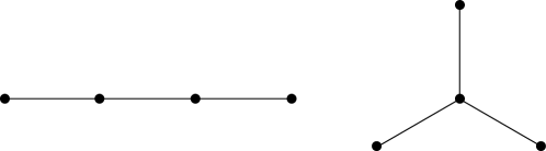
Figure 1: Both graphs have the same magnitude $\displaystyle\frac{4-2q}{1+q}$ $(q=e^{-t})$.

There are many such examples obtained by applying Whitney twist ([4]).

On the other hand, if we restrict ourselves to finte subsets of Euclidean spaces, we can expect magnitude to be a powerful tool for distinguishing spaces, since there are examples of spaces that cannot be distinguished by the discrete version of the natural concept in integral geometry but can be distinguished by magnitude. In fact, numerical experiments shows that the magnitude can distinguish 30 possible positions of four vertices of tetrahedra with the same set of edge lengths $\{7,8,9,10,11,12\}$. Here, the set of edge lengths with multiplicity can be considered as a discrete analogue of the distribution of interpoint distances, which is one of the basic notions in integral geometry. Exchanging the lengths of two edges could change the inverse of the similarity matrix $Z_{X}(t)$ and thus the magnitude. Conceptually speaking, we can say that the magnitude includes not only the edge length information, but also some combinatorial information, which helps us to identify the space.

It should be noted that the distribution of interpoint distances is also useful for identification of spaces. Through the Mellin transform, it yields Brylinski’s beta function, which gives various geometric information such as the volumes of the manifold and its boundary, and integral of curvatures ([10]). Thus the balls and, under certain conditions, the circles and $2$-spheres can be identified by Brylinski’s beta function ([9]). For a convex body (i.e. a compact convex subset of Euclidean space with non-empty interior), the interpoint distance distribution is equivalent to another basic notion in integral geometry, the distribution of chord lengths of the intersection of the convex body and random lines. Blaschke asked ([1] p.51) if the planar domain is determined by the chord length distribution. The answer is no since there is a counterexample ([7]), although Waksman claimed that a sufficiently asymmetric convex polygons is characterized by this distribution ([12]).

In this paper give sufficient conditions for a finite metric space $X$ to be determined by the magnitude function. If the edge lengths are rationally independent, a finite metric space is determined by the asymptotic behavior of the magnitude function at large scale $t\to+\infty$. When $\#X=3$, $X$ is determined by the asymptotic behavior of the magnitude function at small scale $t\to 0^{+}$ without any condition. In the space of the finite metric spaces ([11]), what is excluded by our genericity condition is codimension one and hence measure zero.

Acknowledgement: The author thanks Kiyonori Gomi for helpful suggestions.

2 Main Theorem

Definition 2.1

Let $X$ be a metric space which consists of $n$ points and let $\ell_{1},\dots,\ell_{N}$ be the edge lengths, where $N={n\choose 2}$. A map

$$A\colon\left\{\{i,j\}\,|\,1\leq i<j\leq n\right\}\to\{\ell_{1},\dots,\ell_{N}\}$$

is called combinatorial data (of edge lengths) when there exists a labeling of points in $X$ such that $A(\{i,j\})=d(P_{i},P_{j})$ for any $i,j$ $(i<j)$.

A multiset is a set with multiplicity. We will use the symbol $[\>]$ for multisets. For example, although $\{a,a,b\}$ and $\{a,b\}$ are same as a set, $[a,a,b]$ and $[a,b]$ are different multisets.

Definition 2.2

We say that a finite metric space $X$ is determined by the magnitude function if the multiset of the edge lengths and the combinatorial data are obtained from the magnitude function $M_{X}(t)$.

Recall that the cardinality of a finite metric space is obtained from the magnitude function by $\#X=\lim_{t\to\infty}M_{X}(t)$ ([3] Proposition 2.2.6, [6] Theorem 3).

Definition 2.3

We say that a finite metric space is rationally independent, $p$-generic, where $p$ is a natural number, or satisfying the strict virtual triangle inequality (abbreviated by svti.) condition if the following condition is satisfied respectively:

1. The edge lengths are linearly independent over $\mathbb{Q}$. In other words, the sums of edge lengths do not match for different combinations with multiplicity.

2. The sums of edge lengths do not match for different combinations of $p$ or fewer edges with multiplicity.

3. $\displaystyle\max_{i<j}d_{ij}<2\min_{k<l}d_{kl}$.

Note that the rational independece implies $p$-genericity for any $p$.

Theorem 2.4

A finite metric space $X$ is determined by the magnitude function if $X$ satisfies one of the following conditions ($n=\#X$).

1. $n=3$.

2. $X$ is rationally independent.

3. $X$ is $5$-generic and satisfies the strict virtual triangle inequality condition (svti).

4. $n=4$ and $X$ satisfies the strict virtual triangle inequality condition (svti).

The proof of the theorem yields

Proposition 2.5

The complete graph is determined by the magnitude function.

This can be thought of as a finite-dimensional version of Proposition 3.3. of [2] that a ball is determined by the magnitude function.

Remark 2.6

(1) For any finite metric space $X$ there is a positive number $t_{0}$ such that if $t>t_{0}$ then the similarity matrix $Z_{X}(t)$ is invertible ([3]), in other words, $z_{X}(q)$ $(0<q<1)$ is invertible for sufficiently small $q$.

(2) When $n=3$ the similarity matrix $Z_{X}(t)$ is invertible for any $t$ $(t>0)$ ([3] Proposition 2.4.15).

(3) When $n=4$ the similarity matrix $Z_{X}(t)$ is invertible for any $t$ $(t>0)$ ([8] Theorem 3.6 (4)).

(4) Let $N={n\choose 2}$ as before and put

$$\mathcal{L}_{n}=\left\{(d_{12},\dots,d_{n-1\,n})\in(\mathbb{R}_{>0})^{N}\,\left|\,\begin{array}[]{l}\,d_{ij}+d_{jk}\geq d_{ik}\>\,\forall i,j,k\,(1\leq i,j,k\leq n),\\[1.42262pt] \mbox{where }\>d_{\lambda\lambda}=0,\,d_{\lambda\mu}=d_{\mu\lambda}\end{array}\right.\right\}.$$

The symmetric group $\mathfrak{S}_{n}$ acts on $\mathcal{L}_{n}$ by $\sigma\cdot(d_{ij})=(d_{\sigma(i)\sigma(j)})$. The space of $n$-point metric spaces $\mathcal{M}et_{n}$ can be identified with $\mathcal{L}_{n}/\mathfrak{S}_{n}$ ([11]). Then the metric space $X$ is determined by the magnitude function if and only if $M_{X}(t)$ determines a point in $\mathcal{M}et_{n}$.

Suppose $\mathcal{L}_{n}$ is equipped with the Lebesgue measure and $\mathcal{M}et_{n}$ with the image measure. Then the set of rationally dependent $n$-point metric spaces is measure zero in $\mathcal{M}et_{n}$ since it is a union of countably many codimension one subspaces.

(5) Any graph with graph metric with two edges or more is rationally dependent. Any connected graph except for complete graphs does not satisfy the strict virtual triangle inequality condition.

(6) It can be seen that in the absence of maximum symmetry, moderate asymmetry is more convenient for identifying spaces.

3 Proof of the Theorem

Remark that we have only to prove (2) for $n\geq 4$ and (3) for $n\geq 5$. Some calculations were checked using Maple.

3.1 Asymptotic behavior at small scale when $n=3,4$

The asymptotic behavior of the magnitude function at small scale will be used when $n=3$ and $4$.

Let $\Delta_{X,ij}(t)$ be the $(i,j)$-cofactor of $Z_{X}(t)$. Put

$$M\!u_{X}(t)=\sum_{i,j}\Delta_{X,ij}(t),\quad M\!d_{X}(t)=\det Z_{X}(t),$$

then $M_{X}(t)=M\!u_{X}(t)/M\!d_{X}(t)$.

Let $\nu_{k}=\nu_{k}(d_{ij})$ and $\delta_{k}=\delta_{k}(d_{ij})$ be the coefficients of series expansion of $M\!u_{X}(t)$ and $M\!d_{X}(t)$ respectively: $\displaystyle M\!u_{X}(t)=\sum_{k}\nu_{k}\,t^{k},M\!d_{X}(t)=\sum_{l}\delta_{l}\,t^{l}$. Roff and Yoshinaga ([11]) recently proved

$$\nu_{0}=\dots=\nu_{n-2}=0,\>\delta_{0}=\dots=\delta_{n-2}=0,\>\nu_{n-1}=\delta_{n-1}.$$ (3.1)

Proposition 3.1

1. $\delta_{2}$ is positive for any $3$-point set.

2. $\delta_{3}$ is non-negative for any $4$-point set and positive if strict inequalities hold in all triangle inequalities.

3. $\delta_{3}$ is positive for any $4$-point metric subspace of the Euclidean space with the standard metric.

Proof. (1) Direct calculation shows

$$\delta_{2}=\frac{1}{2}\sum_{\{i,j,k\}=\{1,2,3\}}(d_{jk}+d_{ik}-d_{ij})(d_{ik}+d_{ij}-d_{jk}).$$ (3.2)

Among the three terms of the form $d_{jk}+d_{ik}-d_{ij}$ $(i<j)$ at most only one can be $0$. Hence $\delta_{2}>0$.

(2) Direct calculation shows that $\delta_{3}$ is given by the denominator of (3.19), where $\mathcal{I}_{\triangle}$ is given by (3.7), $\mathcal{I}_{\mbox{\footnotesize$3$-path}}$ by (3.8), and $\mathcal{I}_{\mbox{\footnotesize opp}}$ is same as $\mathcal{I}_{\mbox{\footnotesize disj}}$ given by (3.11), and that it is equal to

$$\frac{1}{6}\sum_{\{i,j,k,l\}=\{1,2,3,4\}}(d_{ik}+d_{jk}-d_{ij})(d_{il}+d_{kl}-d_{ik})(d_{ij}+d_{jl}-d_{il}).$$ (3.3)

(3) The above statement implies that $\delta_{3}$ is positive if none of the triangles collapses. Suppose that one triangle, say $\triangle P_{1}P_{2}P_{3}$ collapses. If $P_{4}$ is not on the line $L$ through $P_{1},P_{2}$ and $P_{3}$, then

$$(d_{24}+d_{12}-d_{14})(d_{34}+d_{23}-d_{24})(d_{14}+d_{13}-d_{34})>0,$$

which implies $\delta_{3}>0$. If $P_{4}$ is on the line $L$, then we may assume without loss of generality that $P_{1},P_{2},P_{3},P_{4}$ lie on $L$ in this order. Then $\delta_{3}=8d_{12}d_{23}d_{34}>0$. $\Box$

Remark 3.2

(1) Proposition 3.1 implies that any $3$-point set and $4$-point set in the Euclid space is generic in the sense of Roff-Yoshinga (Theorem 2.3 of [11]). It gives an alternative direct proof that any $3$-point set and $4$-point set in the Euclid space has one-point property.

(2) The strict triangle inequality condition in (2) is satisfied if either the strict virtual triangle inequality condition or the rational independence condition (ri) is satisfied. Therefore, for $4$-point sets, our condition is stronger (i.e. more restrictive) than Roff-Yoshinga’s genericity condition.

(3) There is an example of a $4$-point metric space that makes $\delta_{3}$ zero, for example, a square graph with graph metric.

(4) A similar equality like (3.2) or (3.3) does not hold when $n=5$. The sign of $\delta_{4}$ may change. In fact, let $X_{3,2;\ell}$ $(0<\ell\leq 2)$ be the space obtained by connecting the vertices on the two-point side of the complete bipartite graph $K_{3,2}$ with an edge of length $\ell$ (Figure 3). Then $\delta_{4}=-4\ell(3\ell-4)$. Note that when $\delta_{4}$ is negative ($4/3<\delta\leq 2$) the magnitude function behaves like that of $K_{3,2}$ (Figure 3).

Remark that this space cannot be isometrically embedded in Eucidean space.

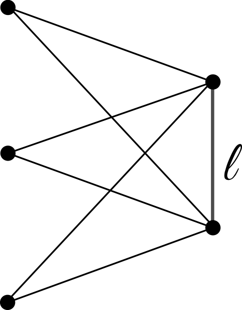
Figure 2: $X_{3,2;\ell}$, the complete bipartite graph $K_{3,2}$ attached an edge with length $\ell$

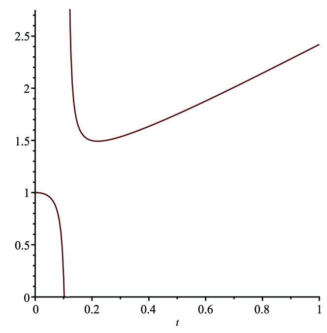
Figure 3: The magnitude function of $X_{3,2;\ell}$ when $\ell=3/2$

Put $\displaystyle M_{\lambda}=\lim_{t\to 0^{+}}\frac{d^{\lambda}}{dt^{\lambda}}M_{X}(t)$ for $\lambda\geq 0$. (3.1) implies that if $\delta_{n-1}\neq 0$ then $M_{1}$ is given by

$$M_{1}=\frac{\nu_{n}-\delta_{n}}{\delta_{n-1}}.$$ (3.4)

3.2 Proof of (1)

The proof of this case is carried out by a different way from the other cases. We only need the asymptotic behavior of the magnitude function at small scale.

Assume $n=3$. Put $a=d_{12},b=d_{13}$ and $c=d_{23}$.

Lemma 3.3

For $\lambda=1,2$ and $3$, $M_{\lambda}=\lim_{t\to 0^{+}}\frac{d^{\lambda}}{dt^{\lambda}}M_{X}(t)$ are given by

$$\begin{array}[]{rcl}M_{1}&=&\displaystyle\frac{2abc}{-a^{2}-b^{2}-c^{2}+2ab+2bc+2ca},\\[17.07164pt] M_{2}&=&\displaystyle\frac{2abc(b+c-a)(c+a-b)(a+b-c)}{{(-a^{2}-b^{2}-c^{2}+2ab+2bc+2ca)}^{2}},\\[17.07164pt] M_{3}&=&\displaystyle\frac{abc\,P(a,b,c)}{{(-a^{2}-b^{2}-c^{2}+2ab+2bc+2ca)}^{3}},\end{array}$$

where

$$\begin{array}[]{rcl}P(a,b,c)&=&\displaystyle a^{6}+\dots+a^{5}b+\dots-13a^{4}b^{2}-\dots+9a^{4}bc+\dots+22a^{3}b^{3}+\dots\\[5.69054pt] &&\displaystyle-10a^{3}b^{2}c-\dots+30a^{2}b^{2}c^{2}.\end{array}$$

Since the denominators of $M_{\lambda}$ are $\delta_{2}^{\lambda}$ they are positive by Proposition 3.1.

Proof. If we put $\sigma_{\mu}=a^{\mu}+b^{\mu}+c^{\mu}$ $(\mu\in\mathbb{N})$, we have

$$\begin{array}[]{c}\nu_{0}=\nu_{1}=\delta_{0}=\delta_{1}=0,\>\nu_{2}=\delta_{2}=\sigma_{1}^{\,2}-2\sigma_{2},\\[8.53581pt] \displaystyle\nu_{3}=-\sigma_{1}\sigma_{2}+2\sigma_{3},\,\nu_{4}=\frac{\sigma_{1}\sigma_{3}}{3}+\frac{\sigma_{2}^{\,2}}{4}-\frac{7\sigma_{4}}{6},\,\nu_{5}=-\frac{\sigma_{1}\sigma_{4}}{12}-\frac{\sigma_{2}\sigma_{3}}{6}+\frac{\sigma_{5}}{2},\\[8.53581pt] \displaystyle\nu_{3}-\delta_{3}=2abc,\>\nu_{4}-\delta_{4}=-abc\,\sigma_{1},\>\nu_{5}-\delta_{5}=\frac{abc}{4}\left(\sigma_{1}^{\,2}+\frac{\sigma_{2}}{3}\right).\end{array}$$

Now $M_{1}$ is obtained from (3.4) and $M_{2}$ from

$$M_{2}=2\,\frac{(\nu_{4}-\delta_{4})\delta_{2}-(\nu_{3}-\delta_{3})\delta_{3}}{\delta_{2}^{\,2}}.$$

$M_{3}$ is obtained in the same way, although the calculation is more complicated, so we omit the details. $\Box$

Lemma 3.4

The edge lengths $a,b$ and $c$ can be obtained from $M_{1},M_{2}$ and $M_{3}$.

Proof. Let $s_{1},s_{2}$ and $s_{3}$ be elementary symmetric polynomials of

$$x=b+c-a,\>y=c+a-b,\>z=a+b-c\,;$$

$$\left\{\begin{array}[]{rcl}s_{1}&=&x+y+z,\\[2.84526pt] s_{2}&=&xy+yz+zx,\\[2.84526pt] s_{3}&=&xyz.\end{array}\right.$$

Since $x,y,z\geq 0$ and at most one of $x,y$ and $z$ can be $0$, $s_{1},s_{2}>0$ and $s_{3}\geq 0$.

Since $M_{1},M_{2}$ and $M_{3}$ are symmetric in $a,b$ and $c$, and the elementary symmetric polynomials of $a,b$ and $c$ can be expressed by $s_{1},s_{2}$ and $s_{3}$ as

$$\left\{\begin{array}[]{rcl}a+b+c&=&s_{1},\\[5.69054pt] ab+bc+ca&=&\displaystyle\frac{s_{1}^{\,2}+s_{2}}{4},\\[11.38109pt] abc&=&\displaystyle\frac{s_{1}s_{2}-s_{3}}{8},\end{array}\right.$$ (3.5)

$M_{1},M_{2}$ and $M_{3}$ can be expressed by $s_{1},s_{2}$ and $s_{3}$;

$$\begin{array}[]{rcl}M_{1}&=&\displaystyle\frac{s_{1}s_{2}-s_{3}}{4s_{2}},\\[11.38109pt] M_{2}&=&\displaystyle\frac{(s_{1}s_{2}-s_{3})s_{3}}{4s_{2}^{\,2}},\\[11.38109pt] M_{3}&=&\displaystyle-\frac{(s_{1}s_{2}-s_{3})\left(s_{1}^{\,2}s_{2}^{\,2}+4s_{1}s_{2}s_{3}-3s_{2}^{\,3}-12s_{3}^{\,2}\right)}{32s_{2}^{\,3}}.\end{array}$$

Remark that $M_{1}>0$ since $s_{1}s_{2}-s_{3}=8abc>0$ and $s_{2}>0$. Solving above equations for $s_{1},s_{2}$ and $s_{3}$, we obtain

$$\begin{array}[]{rcl}s_{1}&=&\displaystyle\frac{4M_{1}^{\,2}+M_{2}}{M_{1}},\\[17.07164pt] s_{2}&=&\displaystyle\frac{16M_{1}^{\,4}+24M_{1}^{\,2}M_{2}+8M_{1}M_{3}-7M_{2}^{\,2}}{3M_{1}^{\,2}},\\[17.07164pt] s_{3}&=&\displaystyle\frac{M_{2}\left(16M_{1}^{\,4}+24M_{1}^{\,2}M_{2}+8M_{1}M_{3}-7M_{2}^{\,2}\right)}{3M_{1}^{\,3}}.\end{array}$$ (3.6)

The edge lengths $a,b$ and $c$ are obtained from $s_{1},s_{2}$ and $s_{3}$ by (3.5), and hence from $M_{1},M_{2}$ and $M_{3}$ by (3.6), which completes the proof. $\Box$

Corollary 3.5

A $3$-point metric space $X$ is determined by $\displaystyle\lim_{t\to 0^{+}}M^{(\lambda)}_{X}(t)$ $(\lambda=1,2,3)$.

3.3 Asymptotic behavior at large scale when $n\geq 4$

In this subsection we investigate the asymptotic behavior of the magnitude function $M_{X}(t)$ at large scale ($t\to+\infty$) as preparation for the proof when $n\geq 4$. For this purpose it seems that the use of the formal magnitude $m_{X}(q)$ $(q=e^{-t})$ would make the description easier to read. Assume $n\geq 4$ in what follows.

(i) First we show that a finite rationally independent metric space is determined by the triples of lengths of three consecutive edges that form triangles or open $3$-paths.

Let $X=\{P_{1},\dots,P_{n}\}$. Let $\widetilde{\mathcal{S}}_{\triangle}$ be the multiset of the multisets of lengths of edges forming triangles:

$$\begin{array}[]{rcl}\mathcal{I}_{\triangle}&=&\{(i,j,k)\,|\,1\leq i<j<k\leq n\},\\[5.69054pt] \widetilde{\mathcal{S}}_{\triangle}&=&\displaystyle\left[\,[d_{ij},d_{jk},d_{ki}]\,|\,(i,j,k)\in\mathcal{I}_{\triangle}\right].\end{array}$$ (3.7)

Note that $\mathcal{I}_{\triangle}$ has no information about the subscripts of $d_{\ast\ast}$; in other words, even if we know the triplet of edge lengths, we do not know their vertices. Let $\widetilde{\mathcal{S}}_{3\mbox{\footnotesize-path}}$ (or $\mathcal{S}_{3\mbox{\footnotesize-path}}$) be the multiset of the multisets of lengths of edges forming open $3$-paths (or respectively, with the information of the length of the middle edge):

$$\mathcal{I}_{3\mbox{\footnotesize-path}} = \displaystyle\left\{(i,j,k,l)\,|\,1\leq i,j,k,l\leq n,\,i\neq j\neq k\neq l\neq i,\,i<l\right\},$$ (3.8)

$$\widetilde{\mathcal{S}}_{3\mbox{\footnotesize-path}} = \displaystyle\left[\,[d_{ij},d_{jk},d_{kl}]\,|\,(i,j,k,l)\in\mathcal{I}_{3\mbox{\footnotesize-path}}\right],$$

$$\mathcal{S}_{3\mbox{\footnotesize-path}} = \displaystyle\left[(d_{jk},[d_{ij},d_{kl}])\,|\,(i,j,k,l)\in\mathcal{I}_{3\mbox{\footnotesize-path}}\right].$$

Lemma 3.6

A finite $3$-generic metric space is determined by $\widetilde{\mathcal{S}}_{\triangle}$ and $\widetilde{\mathcal{S}}_{3\mbox{\rm\footnotesize-path}}$.

Proof. The $3$-genericity condition ($\mbox{g}_{3}$) implies that the edge lengths are different from each other. Therefore from $\widetilde{\mathcal{S}}_{\triangle}$ (or $\widetilde{\mathcal{S}}_{3\mbox{\footnotesize-path}}$) we can obtain the multiset of the edge lengths $\widetilde{\mathcal{S}}_{1}=[d_{ij}\,|\,1\leq i<j\leq n]$ (in fact it is a set in this case).

Note that the data of $\widetilde{\mathcal{S}}_{\triangle}$ and $\widetilde{\mathcal{S}}_{3\mbox{\footnotesize-path}}$ produce $\mathcal{S}_{3\mbox{\footnotesize-path}}$, namely, the information of the middle edges of open $3$-paths can be obtained from $\widetilde{\mathcal{S}}_{\triangle}$ and $\widetilde{\mathcal{S}}_{3\mbox{\footnotesize-path}}$. This is because the two edges at the ends of an open $3$-path cannot form a triangle with another edge.

Suppose we have the data of $\widetilde{\mathcal{S}}_{1},\widetilde{\mathcal{S}}_{\triangle}$ and $\mathcal{S}_{3\mbox{\footnotesize-path}}$. Choose a triangle and an edge of it. We may label the three vertices $P_{1},P_{2}$ and $P_{3}$ so that the edge we selected is $P_{1}P_{2}$. Let $\ell_{\alpha}=d(P_{2},P_{3}),\ell_{\beta}=d(P_{3},P_{1})$ and $\ell_{\gamma}=d(P_{1},P_{2})$. There are still $n-3$ triangles containing the edge $P_{1}P_{2}$. There are two ways to attach each triangle to $P_{1}P_{2}$, but one is determined from the information of open 3-paths and middle edges as follows. Suppose $[\ell_{\lambda},\ell_{\mu},\ell_{\gamma}]\in\widetilde{\mathcal{S}}_{\triangle}$. Let the remaining vertex be $P_{4}$, say. Note that both $\ell_{\lambda},\ell_{\mu},\ell_{\alpha}$ and $\ell_{\lambda},\ell_{\mu},\ell_{\beta}$ form open $3$-paths. If the middle edge of $\ell_{\lambda},\ell_{\mu},\ell_{\alpha}$ is $\ell_{\lambda}$ then the triangle $\triangle P_{4}P_{1}P_{2}$ is attached to the edge $P_{1}P_{2}$ in a way that $d(P_{4},P_{1})=\ell_{\mu}$ and $d(P_{4},P_{2})=\ell_{\lambda}$, and if not the other way.

After attaching the remaining $n-4$ triangles to $P_{1}P_{2}$, label the remaining vertices $P_{5},\dots,P_{n}$. The lengths $d(P_{i},P_{1}),d(P_{i},P_{2})$ $(4\leq i\leq n)$ are determinded by the procedure described above. The length $d(P_{i},P_{j})$ $(3\leq i<j\leq n)$ is determined as the unique element $\ell$ in $\widetilde{\mathcal{S}}_{1}$ such that $[\ell,d(P_{i},P_{1}),d(P_{j},P_{1})]$ is an element of $\widetilde{\mathcal{S}}_{\triangle}$. $\Box$

(ii) Next we prepare a lemma which we will use to get a multiset consisting of the sums of lengths of edges forming triangles and a multiset consisting of the sums of lengths of edges forming open $3$-paths from the formal magnitude $m_{X}(q)$.

Let $w_{X,ij}(q)$ be the $(i,j)$-cofactor of $z_{X}(q)$. Put

$$mu_{X}(q)=\sum_{i,j}w_{X,ij}(q),\quad md_{X}(q)=\det z_{X}(q),$$

then we have $m_{X}(q)=mu_{X}(q)/md_{X}(q)$.

Note that both $mu_{X}(q)$ and $md_{X}(q)$ are generalized polynomials with real exponents and integer coefficients. Let $\mathcal{P}_{all}$ be the commutative monoid generated by $\widetilde{\mathcal{S}}_{1}=[d_{ij}]$;

$$\mathcal{P}_{all}=\Bigg{\{}\sum_{i<j}a_{ij}d_{ij}\,|\,a_{ij}\in\mathbb{Z},a_{ij}\geq 0\Bigg{\}},$$ (3.9)

then the exponent of any term that appears in $mu_{X}(q)$ or $md_{X}(q)$ belongs to $\mathcal{P}_{all}$.

Definition 3.7

1. We define the $d$-index of a term $q^{\,\sum_{i<j}a_{ij}d_{ij}}$ to be $\sum_{i<j}a_{ij}$.

2. Let $mu_{X,3}(q)$ (or $md_{X,3}(q)$) be the sum of all the terms in $mu_{X}(q)$ (or resplectively $md_{X}(q)$) with the $d$-index less than or equal to $3$.

Lemma 3.8

We have

$$md_{X,3}(q) = \displaystyle 1-\sum_{i<j}q^{2d_{ij}}+2\sum_{\mathcal{I}_{\triangle}}q^{d_{ij}+d_{jk}+d_{ki}},$$

$$mu_{X,3}(q) = \displaystyle n-2\sum_{i<j}q^{d_{ij}}-(n-2)\sum_{i<j}q^{2d_{ij}}+\sum_{\mathcal{I}_{\mbox{\rm\scriptsize$2$-path}}}q^{d_{ij}+d_{jk}}$$ (3.10)

$$\displaystyle+2(n-3)\sum_{\mathcal{I}_{\triangle}}q^{d_{ij}+d_{jk}+d_{ki}}-2\sum_{\mathcal{I}_{\mbox{\rm\scriptsize$3$-path}}}q^{d_{ij}+d_{jk}+d_{kl}}$$

$$\displaystyle+2\sum_{\mathcal{I}_{\mbox{\rm\scriptsize disj}}}\left(q^{2d_{ij}+d_{kl}}+q^{d_{ij}+2d_{kl}}\right),$$

where

$$\mathcal{I}_{2\mbox{\rm\footnotesize-path}} = \displaystyle\left\{(i,j,k)\,|\,i\neq j\neq k,\,i<k\right\},$$

$$\mathcal{I}_{\mbox{\rm\footnotesize disj}} = \displaystyle\left\{(i,j,k,l)\,|\,i<j,k<l,\{i,j\}\cap\{k,l\}=\emptyset,\,i<k\right\}.$$ (3.11)

Proof. (1) $md_{X,3}(q)$. Terms with $d$-index $3$ or less are those in which three or less of the $1$’s arranged on the diagonal of $z_{X}(q)$ are not used when calculating the determinant. When the unused $1$’s are some of the three in the upper left corner, the terms in question become the minor of the upper left $3\times 3$ submatrix of

$$z_{X}(q)=\left(\begin{array}[]{ccccc}1&q^{d_{12}}&q^{d_{13}}&\dots&\\[2.84526pt] q^{d_{12}}&1&q^{d_{23}}&\dots&\\[2.84526pt] q^{d_{13}}&q^{d_{23}}&1&\dots&\\[2.84526pt] \vdots&\vdots&\vdots&\ddots&\\[2.84526pt] &&&&\>1\end{array}\right),$$

which is given by $-d_{12}^{\,2}-d_{13}^{\,2}-d_{23}^{\,2}+2d_{12}d_{13}d_{23}$. From this the conclusion follows.

(2) $mu_{X,3}(q)$. When $i=j$, the sum of the terms of $w_{X,ii}(q)$ with $d$-index $3$ or less, which we denote by $w_{X,ii,3}(q)$, can be computed similarly to $md_{X,3}(q)$:

$$w_{X,ii,3}(q)=1-\sum_{j<k,\{j,k\}\not\ni i}q^{2d_{jk}}+2\sum_{j<k<l,\{j,k,l\}\not\ni i}q^{d_{jk}+d_{kl}+d_{lj}},$$

which implies

$$\sum_{i}w_{X,ii,3}(q)=n-(n-2)\sum_{i<j}q^{2d_{ij}}+2(n-3)\sum_{\mathcal{I}_{\triangle}}q^{d_{ij}+d_{jk}+d_{ki}}.$$ (3.12)

On the other hand, when $i\neq j$, there are no more than two unused $1$’s. Bringing the two $1$’s to the top left by applying the same permutation to the rows and columns, we have

$$w_{X,ij}=\displaystyle-\left|\begin{array}[]{cccc}q^{d_{ij}}&q^{d_{jk}}&q^{d_{jl}}&\\[2.84526pt] q^{d_{ik}}&1&q^{d_{kl}}&\\[2.84526pt] q^{d_{il}}&q^{d_{kl}}&1&\\ &&&\ddots\end{array}\right|\qquad(k<l,\{k,l\}\cap\{i,j\}=\emptyset),$$

which implies that the sum of the terms with $d$-index $\leq 3$ is given by

$$w_{X,ij,3} = \displaystyle-q^{d_{ij}}+\sum_{k<l,\{k,l\}\cap\{i,j\}=\emptyset}\left(q^{d_{ik}+d_{kj}}+q^{d_{il}+d_{lj}}\right)$$ (3.14)

$$\displaystyle+\sum_{k<l,\{k,l\}\cap\{i,j\}=\emptyset}\left(-q^{d_{ik}+d_{kl}+d_{lj}}-q^{d_{il}+d_{lk}+d_{kj}}+q^{2d_{kl}+d_{ij}}\right).\qquad{\phantom{a}}$$

The last two terms of (3.14), the first two terms of (3.14), and the last term of (3.14) give the “$2$-path” terms, the “open $3$-path” terms, and the “disjoint” terms of (3.10) respectively. Hence, together with (3.12), it completes the proof. $\Box$

Put $\xi(q)=md_{X}(q)-1$ then $m_{X}(q)$ is expressed by the generalized formal power series with real exponents and integer coefficients

$$m_{X}(q)=mu_{X}(q)\left(1-\xi(q)+\xi(q)^{2}-\dots\right).$$

As a function of $q$, since $\xi(q)$ tends to $0$ as $q$ approaches $0^{+}$, the right hand side above converges for sufficiently small $q$. Since both $mu_{X}(q)$ and $\xi(q)$ are generalized polynomials whose exponents belong to $\mathcal{P}_{all}$ given by (3.9), the exponents of $m_{X}(q)$ also belong to $\mathcal{P}_{all}$. Let $\mathcal{P}$ $(\mathcal{P}\subset\mathcal{P}_{all})$ be the set of positive exponents that appear in $m_{X}(q)$.

Lemma 3.9

Let $m_{X,3}(q)$ be the sum of all the terms in $m_{X}(q)$ with the $d$-index less than or equal to $3$. Then it is given by

$$m_{X,3}(q) = \displaystyle n-2\sum_{i<j}q^{d_{ij}}+2\sum_{i<j}q^{2d_{ij}}+2\sum_{\mathcal{I}_{\mbox{\rm\scriptsize$2$-path}}}q^{d_{ij}+d_{jk}}-2\Bigg{(}\sum_{i<j}q^{2d_{ij}}\Bigg{)}\left(\sum_{k<l}q^{d_{kl}}\right)$$

$$\displaystyle-6\sum_{\mathcal{I}_{\triangle}}q^{d_{ij}+d_{jk}+d_{ki}}-2\sum_{\mathcal{I}_{\mbox{\rm\scriptsize$3$-path}}}q^{d_{ij}+d_{jk}+d_{kl}}+2\sum_{\mathcal{I}_{\mbox{\rm\scriptsize disj}}}\left(q^{2d_{ij}+d_{kl}}+q^{d_{ij}+2d_{kl}}\right).$$

Proof. Since any term of $\xi(q)$ has $d$-index $\geq 2$, $m_{X,3}(q)$ can be obtained from $mu_{X}(q)(1-\xi(q))$ by collecting terms with $d$-index $\leq 3$. $\Box$

(iii) Finaly we give a lemma to obtain the exponents and coefficients of $m_{X}(q)$ from the magnitude function $M_{X}(t)$.

Lemma 3.10

Suppose $m_{X}(q)$ is expressed as

$$m_{X}(q)=\sum_{m=0}^{\infty}a_{m}q^{\alpha_{m}}\quad(a_{m}\in\mathbb{R},\,\{\alpha_{0},\alpha_{1}.\dots\}=\mathcal{P},\,\alpha_{0}<\alpha_{1}<\dots).$$

Then $\alpha_{0}=0$ and $\displaystyle a_{0}=\lim_{t\to+\infty}M_{X}(t)=\#X$, and $\alpha_{m}$ and $a_{m}$ are given inductively by

$$\begin{array}[]{rcl}\alpha_{m}&=&\displaystyle\lim_{t\to+\infty}\frac{\displaystyle\left|\log\left(M_{X}(t)-\sum_{i=0}^{m-1}a_{i}\,e^{-t\alpha_{i}}\right)\right|}{t},\\[17.07164pt] a_{m}&=&\displaystyle\lim_{t\to+\infty}e^{t\alpha_{m}}\left(M_{X}(t)-\sum_{i=0}^{m-1}a_{i}\,e^{-t\alpha_{i}}\right).\end{array}$$

3.4 Proof of (2)

By Lemma 3.10 we obtain the multiset $\mathcal{P}$ from $M_{X}(t)$. From $\mathcal{P}$ we can obtain the multiset of the edge lengths $\widetilde{\mathcal{P}}_{1}=[d_{12},\dots,d_{n-1n}]$ as follows. Remark that the rational independenc condition (ri) implies that $d_{ij}$’s are all different from each other, hence $\widetilde{\mathcal{P}}_{1}$ is an ordinary set in fact. Define $\ell_{1},\dots,\ell_{N}$ inductively, where $N={n\choose 2}$, by

$$\begin{array}[]{l}\displaystyle\ell_{1}=\min\mathcal{P},\\[5.69054pt] \displaystyle\ell_{2}=\min\left(\mathcal{P}\setminus\{\tau\,\ell_{1}\,|\,\tau\in\mathbb{N}\}\right),\\[5.69054pt] \displaystyle\ell_{3}=\min\left(\mathcal{P}\setminus\{\tau_{1}\,\ell_{1}+\tau_{2}\,\ell_{2}\,|\,\tau_{1},\tau_{2}\in\mathbb{N}\cup\{0\}\}\right),\\[5.69054pt] \dots\end{array}$$

Then the (multi)set of edge lengths $\widetilde{\mathcal{P}}_{1}$ is given by the (multi)set $[\ell_{1},\dots,\ell_{N}]$.

Put

$$\begin{array}[]{rcl}\widetilde{\mathcal{S}}_{p}&=&\displaystyle[\,[\ell_{\alpha_{i_{1}}},\dots,\ell_{\alpha_{i_{p}}}]\,|\,1\leq\alpha_{i_{1}}\leq\dots\leq\alpha_{i_{p}}\leq N]\qquad(p\in\mathbb{N}),\\[5.69054pt] \widetilde{\mathcal{S}}&=&\displaystyle\bigcup_{p\in\mathbb{N}}\widetilde{\mathcal{S}}_{p}.\end{array}$$

Note that $\widetilde{\mathcal{S}}_{1}=\widetilde{\mathcal{P}}_{1}$ and that $\widetilde{\mathcal{S}}_{3}\supset\widetilde{\mathcal{S}}_{\triangle},\widetilde{\mathcal{S}}_{3\mbox{\footnotesize-path}}$. The rational independenc condition (ri) implies that a map $\Sigma\colon\widetilde{\mathcal{S}}\to\mathbb{R}$ given by

$$\Sigma\left(\,[\ell_{\alpha_{i_{1}}},\dots,\ell_{\alpha_{i_{p}}}]\,\right)=\ell_{\alpha_{i_{1}}}+\dots+\ell_{\alpha_{i_{p}}}$$

is injective. Since the “triangle” terms and the “open $3$-path” terms in (LABEL:m_3) have different coefficients, by comparing $\mathcal{P}$ and $\Sigma(\widetilde{\mathcal{S}}_{3}^{\circ})$, where $\widetilde{\mathcal{S}}_{3}^{\circ}=[\,[\ell_{\alpha_{1}},\ell_{\alpha_{2}},\ell_{\alpha_{3}}]\,|\,1\leq\alpha_{1}<\alpha_{2}<\alpha_{3}\leq N]$, we obtain $\Sigma(\widetilde{\mathcal{S}}_{\triangle})$ and $\Sigma(\widetilde{\mathcal{S}}_{3\mbox{\footnotesize-path}})$. Since $\Sigma$ is injective, the conclusion follows from Lemma 3.6.

3.5 Proof of (3)

The proof is almost the same as the previous case.

The strict virtual triangle inequality condition implies $\max_{1\leq\alpha\leq N}\ell_{\alpha}<\min\cup_{p\geq 2}\,\Sigma(\widetilde{\mathcal{S}}_{p})$, hence $\ell_{\alpha}$ $(1\leq\alpha\leq N)$ can be determined as the first $N$ smallest numbers of $\mathcal{P}$. Since the strict virtual triangle inequality condition implies $\Sigma(\widetilde{\mathcal{S}}_{3})\,\cap\,\cup_{p\geq 6}\,\Sigma(\widetilde{\mathcal{S}}_{p})=\emptyset$ and the $5$-genericity condition ($\mbox{g}_{5}$) implies $\Sigma\colon\cup_{p\leq 5}\Sigma(\widetilde{\mathcal{S}}_{p})\to\mathbb{R}$ is injective, we obtain $\Sigma(\widetilde{\mathcal{S}}_{\triangle})$ and $\Sigma(\widetilde{\mathcal{S}}_{3\mbox{\footnotesize-path}})$. The rest of the proof is same as in the previous case.

3.6 Proof of (4)

When the number of points is four, each edge has exactly one disjoint edge, which we call the opposite edge, and accordingly, $\mathcal{I}_{\mbox{\footnotesize disj}}$ will be denoted by $\mathcal{I}_{\mbox{\footnotesize opp}}$ hereafter. Note that a four point set has three pairs of opposite edges.

Without the rational independenc condition, it can happen that the combination of edges cannot be determined from $m_{X}(q)$, as was the case in the example of graphs in the Introduction (Figure 1). This complicates the proof.

Suppose we know the generalized formal power series expression of $m_{X}(q)$. The proof consists of the following four steps.

1. The multiset of the edge lengths is determined.

2. The multiset of the sums of lengths of pairs of opposite edges is determined.

3. The combination of opposite edges that give the sums mentioned above is determined.

4. One of the two possible “tetrahedra” is determined.

Step 1. The strict virtual triangle inequality condition implies that the multiset of the edge lengths $\widetilde{\mathcal{P}}_{1}=[\ell_{1},\dots,\ell_{6}]$ $(\ell_{1}\leq\dots\leq\ell_{6})$ is obtained by taking $N$ numbers with multiplicity from $\mathcal{P}$, increasing from the smallest. The multiplicity can be determined by the coefficient of $q^{d_{ij}}$ in $m_{X}(q)$ divided by $-2$.

Step 2. Put for $p=1,2$ and $3$

$$\sigma_{p}(q)=\sum_{i<j}q^{p\,d_{ij}}=q^{p\,\ell_{1}}+\dots+q^{p\,\ell_{6}}.$$

Define $f(q)$ by modifying $m_{X}(q)$ as

$$f=m_{X}-4+2\sigma_{1}-\sigma_{1}^{2}-\sigma_{2}+\sigma_{1}\sigma_{2}+\frac{1}{3}\sigma_{1}^{3}+\frac{2}{3}\sigma_{3}.$$ (3.16)

Assume that the terms of $f(q)$ are in order of increasing power. Let $f_{3}(q)$ be the sum of all the terms appearing in $f(q)$ with $d$-index less than or equal to $3$. (LABEL:m_3) implies that $f_{3}(q)$ is given by

$$\begin{array}[]{rcl}f_{3}(q)&=&\displaystyle-2\sum_{\mathcal{I}_{\mbox{\scriptsize opp}}}q^{d_{ij}+d_{kl}}\\[17.07164pt] &&\displaystyle-4\sum_{\mathcal{I}_{\triangle}}q^{d_{ij}+d_{jk}+d_{ki}}+2\sum_{\mathcal{I}_{\mbox{\scriptsize vtx}}}q^{d_{ij}+d_{ik}+d_{il}}+2\sum_{\mathcal{I}_{\mbox{\scriptsize opp}}}\left(q^{2d_{ij}+d_{kl}}+q^{d_{ij}+2d_{kl}}\right),\end{array}$$ (3.17)

where

$$\mathcal{I}_{\mbox{\footnotesize vtx}}=\{(i,j,k,l)\,|\,1\leq i\leq 4,\,j<k<l,\,\{j,k,l\}=\{1,2,3,4\}\setminus\{i\}\}.$$

Claim 3.11

Assume $(i,j,k,l)\in\mathcal{I}_{\mbox{\rm\footnotesize opp}}$. Then the following holds.

1. $d_{ij}+d_{kl}<d_{i^{\prime}j^{\prime}}+d_{i^{\prime}k^{\prime}}+d_{i^{\prime}l^{\prime}}$ for any $(i^{\prime},j^{\prime},k^{\prime},l^{\prime})\in\mathcal{I}_{\triangle}$.

2. $d_{ij}+d_{kl}<d_{i^{\prime}j^{\prime}}+d_{i^{\prime}k^{\prime}}+d_{i^{\prime}l^{\prime}}$ for any $(i^{\prime},j^{\prime},k^{\prime},l^{\prime})\in\mathcal{I}_{\mbox{\rm\footnotesize vtx}}$.

3. $d_{ij}+d_{kl}$ is smaller than the exponent of any term of $f(q)$ with $d$-index $4$ or more.

Proof. (1) Any pair of opposite edges has exactly one edge in common with three edges of any triangle. The remaining inequality is a consequence of the strict virtual triangle inequality.

(2) Any pair of opposite edges has exactly one edge in common with three edges having one common vertex.

(3) Consequence of the strict virtual triangle inequality. $\Box$

Put

$$\begin{array}[]{rcl}\widetilde{\mathcal{P}}_{\rm opp,2}&=&\displaystyle[d_{ij}+d_{kl}\,|\,(i,j,k,l)\in\mathcal{I}_{\rm opp}],\\[5.69054pt] \widetilde{\mathcal{P}}_{\rm opp,3}&=&\displaystyle[2d_{ij}+d_{kl},d_{ij}+2d_{kl}\,|\,(i,j,k,l)\in\mathcal{I}_{\rm opp}].\end{array}$$

Lemma 3.12

Let $[\ell_{1},\dots,\ell_{6}]$ be the multiset of edge lengths. If two elements of $\widetilde{\mathcal{P}}_{\rm opp,2}$ appear in $\widetilde{\mathcal{P}}_{\rm opp,3}$, we can find $\alpha,\beta,\gamma,\delta,\lambda,\mu$ that satisfy the followings;

1. $\{\alpha,\beta,\gamma,\delta,\lambda,\mu\}=\{1,2,3,4,5,6\}$,

   $\ell_{\alpha}\leq\ell_{\beta},\ell_{\gamma}\leq\ell_{\delta},\ell_{\lambda}\leq\ell_{\mu}$, $\ell_{\alpha}+\ell_{\beta}\leq\ell_{\gamma}+\ell_{\delta}\leq\ell_{\lambda}+\ell_{\mu}$,

2. $\ell_{\alpha}+\ell_{\beta}=(\ell_{1}+\dots+\ell_{6})/4$,

3. $\ell_{\gamma}+\ell_{\delta}=2\ell_{\alpha}+\ell_{\beta}$ and $\ell_{\lambda}+\ell_{\mu}=\ell_{\alpha}+2\ell_{\beta}$.

Proof. First note that (2) is a consequence of (3).

We may assume without loss of generality that $\widetilde{\mathcal{P}}_{\rm opp,2}$ is given by $[\ell_{\alpha}+\ell_{\beta},\ell_{\gamma}+\ell_{\delta},\ell_{\lambda}+\ell_{\mu}]$ with condition (1) above. Since the smallest element $\ell_{\alpha}+\ell_{\beta}$ cannot appear in $\widetilde{\mathcal{P}}_{\rm opp,3}$, it is enough to show that the case

$$\begin{array}[]{rcl}\ell_{\gamma}+\ell_{\delta}&=&2\ell_{\alpha}+\ell_{\beta}\quad\mbox{ or }\quad\ell_{\alpha}+2\ell_{\beta},\\[5.69054pt] \ell_{\lambda}+\ell_{\mu}&=&2\ell_{\gamma}+\ell_{\delta}\quad\mbox{ or }\quad\ell_{\gamma}+2\ell_{\delta}\end{array}$$ (3.18)

cannot happen.

Assume (3.18). By the strict virtual triangle inequality condition we have $\ell_{\gamma}>(\ell_{\gamma}+\ell_{\delta})/3$, which implies $\ell_{\lambda}+\ell_{\mu}>\frac{4}{3}(\ell_{\gamma}+\ell_{\delta})$. Put $t=\ell_{\alpha}/(\ell_{\alpha}+\ell_{\beta})$. the assumption $\ell_{\alpha}\leq\ell_{\beta}$ and the strict virtual triangle inequality condition imply $1/3<t\leq 1/2$. Therefore we have

$$\ell_{\lambda}+\ell_{\mu}>\frac{4}{3}(\ell_{\gamma}+\ell_{\delta})\geq\frac{4}{3}(t+1)(\ell_{\alpha}+\ell_{\beta})=\frac{4(t+1)}{3t}\ell_{\alpha},$$

which implies

$$\ell_{\mu}\geq\frac{1}{2}(\ell_{\lambda}+\ell_{\mu})>\frac{2}{3}\left(1+\frac{1}{t}\right)\ell_{\alpha}.$$

On the other hand, since $t\leq 1/2$, it means $\ell_{\mu}>2\ell_{\alpha}$, which contradicts the strict virtual triangle inequality condition. $\Box$

We remark that if (1), (2) and (3) of Lemma 3.12 are satisfied then $\ell_{\lambda}+\ell_{\mu}$ cannot be equal to either $2\ell_{\gamma}+\ell_{\delta}$ or $\ell_{\gamma}+2\ell_{\delta}$ by the strict virtual triangle inequality condition.

Proposition 3.13

The multiset of the sums of edge lengths of pairs of opposite edges, $\widetilde{\mathcal{P}}_{\rm opp,2}=\displaystyle[d_{ij}+d_{kl}\,|\,(i,j,k,l)\in\mathcal{I}_{\rm opp}]$ can be obtained from the generalized formal power series expression of $m_{X}(q)$.

Proof. Since it is impossible that all the three elements of $\widetilde{\mathcal{P}}_{\rm opp,2}$ appear in $\widetilde{\mathcal{P}}_{\rm opp,3}$, there are only two possibilities:

Case 1. At most one element of $\widetilde{\mathcal{P}}_{\rm opp,2}$ appears in $\widetilde{\mathcal{P}}_{\rm opp,3}$.

Case 2. Two elements of $\widetilde{\mathcal{P}}_{\rm opp,2}$ appear in $\widetilde{\mathcal{P}}_{\rm opp,3}$.

First we show that if either Case 1 or Case 2 is known in advance, in each case $\widetilde{\mathcal{P}}_{\rm opp,2}$ can be obtained from $f(q)$. Assume $f(q)$ is arranged in increasing powers of $q$.

Case 1. Claim 3.11 implies that at least two of the terms $q^{d_{ij}+d_{kl}}$, where $(i,j,k,l)\in\mathcal{I}_{\mbox{\footnotesize opp}}$, in (3.17) survive, i.e. the coefficients do not cancel out. Take the first term in $f(q)$ with coefficient $-4$ if exists or if not the first two terms with coefficient $-2$. Then the exponent(s) give(s) two elements of $\widetilde{\mathcal{P}}_{\rm opp,2}$. The remaining one element can be obtained by subtracting the sum of the two from $\ell_{1}+\dots+\ell_{6}$.

Case 2. The first term of $f(q)$ has coefficient $-2$ and exponent $\ell_{a}+\ell_{\beta}$ in Lemma 3.12. The strict virtual triangle inequality condition implies that if there are two pairs $\{\alpha,\beta\}$ $(\alpha\neq\beta)$ and $\{\alpha^{\prime},\beta^{\prime}\}$ $(\alpha^{\prime}\neq\beta^{\prime})$ with

$$\ell_{\alpha}+\ell_{\beta}=\ell_{\alpha^{\prime}}+\ell_{\beta^{\prime}}=\frac{\ell_{1}+\dots+\ell_{6}}{4}$$

then $\#\{\alpha,\beta,\alpha^{\prime},\beta^{\prime}\}\leq 3$, namely, the values of $\ell_{\alpha}$ and $\ell_{\beta}$ in Lemma 3.12 are fixed. Then the remaining two elements of $\widetilde{\mathcal{P}}_{\rm opp,2}$ can be obtained by $2\ell_{\alpha}+\ell_{\beta}$ and $\ell_{\alpha}+2\ell_{\beta}$.

Next we show that it can be determined whether Case 1 or Case 2 is occurring from the information of $f(q)$. In fact, Case 2 can occur if and only if the following conditions are all satisfied.

($\ast$) The coefficient of the first term of $f(q)$ is equal to $-2$. The exponent of this term is given by $\ell_{\alpha}+\ell_{\beta}$ for som $\alpha$ and $\beta$ $(\alpha\neq\beta)$. We can choose $\gamma,\delta,\lambda,\mu$ such that $\{\gamma,\delta,\lambda,\mu\}=\{1,\dots,6\}\setminus\{\alpha,\beta\}$ and $\ell_{\gamma}+\ell_{\delta}=2\ell_{\alpha}+\ell_{\beta}$ and $\ell_{\lambda}+\ell_{\mu}=\ell_{\alpha}+2\ell_{\beta}$ hold. There is no term with exponent $\ell_{\gamma}+\ell_{\lambda},\ell_{\gamma}+\ell_{\mu},\ell_{\delta}+\ell_{\lambda}$ or $\ell_{\delta}+\ell_{\mu}$ with coefficient $-2$ or $-4$ in $f(q)$. $\Box$

Step 3. Given a multiset of edge length $\widetilde{\mathcal{P}}_{1}=[\ell_{1},\dots,\ell_{6}]$ $(\ell_{1}\leq\dots\leq\ell_{6})$ and a multiset of the sums of opposite edges $\widetilde{\mathcal{P}}_{\rm opp,2}$, if the combination of opposite edges that realizes the sums is not unique, there are only the following two cases.

1. $\ell_{2}-\ell_{1}=\ell_{5}-\ell_{4}$ and $\ell_{3}-\ell_{2}=\ell_{6}-\ell_{5}$. Then

   $$(\ell_{1}+\ell_{5},\ell_{3}+\ell_{4},\ell_{2}+\ell_{6})=(\ell_{2}+\ell_{4},\ell_{1}+\ell_{6},\ell_{3}+\ell_{5}).$$

2. $\ell_{2}-\ell_{1}=\ell_{4}-\ell_{3}=\ell_{6}-\ell_{5}$. Then

   $$(\ell_{1}+\ell_{4},\ell_{2}+\ell_{5},\ell_{3}+\ell_{6})=(\ell_{2}+\ell_{3},\ell_{1}+\ell_{6},\ell_{4}+\ell_{5}).$$

Case 1. Let ${\rm COMB1}=[\ell_{1}+\ell_{5},\ell_{3}+\ell_{4},\ell_{2}+\ell_{6}]$ and ${\rm COMB2}=[\ell_{2}+\ell_{4},\ell_{1}+\ell_{6},\ell_{3}+\ell_{5}]$. Each combination has two possible configurations as illustrated in Figure 4.

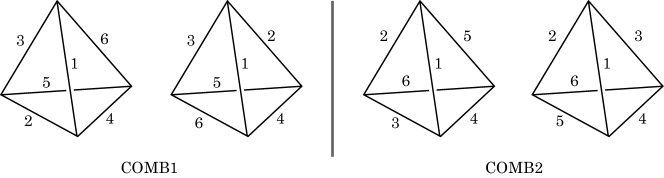
Figure 4: Four possible configurations. $i$ stands for $\ell_{i}$.

Define $g(q)$ by $g(q)=f(q)+2\sum_{\mathcal{I}_{\mbox{\scriptsize opp}}}q^{d_{ij}+d_{kl}}$, where $f$ is given by (3.16), and let $g_{3}(q)$ be the sum of all the terms in $g(q)$ with $d$-index less than or equal to $3$. Then (3.17) implies

$$g_{3}(q)=-4\sum_{\mathcal{I}_{\triangle}}q^{d_{ij}+d_{jk}+d_{ki}}2\sum_{\mathcal{I}_{\mbox{\scriptsize vtx}}}q^{d_{ij}+d_{ik}+d_{il}}+2\sum_{\mathcal{I}_{\mbox{\scriptsize opp}}}\left(q^{2d_{ij}+d_{kl}}+q^{d_{ij}+2d_{kl}}\right).$$

In each configuration in Figure 4, three edges labelled $1,2$ and $3$ form either a triangle or a “Y shape”, hence $\ell_{1}+\ell_{2}+\ell_{3}$ always appears as the exponent of either a “triangle” or a “vertex” term in $g_{3}(q)$ as long as the coefficient does not cancel out with the coefficients of other terms.

Lemma 3.14

$\ell_{1}+\ell_{2}+\ell_{3}$ is the smallest exponent that appears in $g(q)$.

Put $u=\ell_{4}-\ell_{3},v=\ell_{2}-\ell_{1}=\ell_{5}-\ell_{4},w=\ell_{3}-\ell_{2}=\ell_{6}-\ell_{5}$ $(u,v,w\geq 0)$.

Proof. First note that $\ell_{1}+\ell_{2}+\ell_{3}$ is the minimum of $\ell_{i}+\ell_{j}+\ell_{k}$ with $i\neq j\neq k\neq i$, hence it gives the minimum of

$$\{d_{ij}+d_{ik}+d_{il}\,|\,(i,j,k,l)\in\mathcal{I}_{\mbox{\footnotesize vtx}}\}\cup\{d_{ij}+d_{jk}+d_{ki}\,|\,(i,j,k)\in\mathcal{I}_{\triangle}\}.$$

Next since

$$\begin{array}[]{l}COMB1\colon\,\left\{\begin{array}[]{rcl}2\ell_{1}+\ell_{5}&=&\ell_{1}+\ell_{2}+\ell_{3}+u,\\ 2\ell_{2}+\ell_{6}&=&\ell_{1}+\ell_{2}+\ell_{3}+u+2v+w,\\ 2\ell_{3}+\ell_{4}&=&\ell_{1}+\ell_{2}+\ell_{3}+u+v+2w,\end{array}\right.\\[22.76219pt] COMB2\colon\,\left\{\begin{array}[]{rcl}2\ell_{2}+\ell_{4}&=&\ell_{1}+\ell_{2}+\ell_{3}+u+v,\\ 2\ell_{1}+\ell_{6}&=&\ell_{1}+\ell_{2}+\ell_{3}+u+w,\\ 2\ell_{3}+\ell_{5}&=&\ell_{1}+\ell_{2}+\ell_{3}+u+2v+2w,\end{array}\right.\end{array}$$

we have

$$\ell_{1}+\ell_{2}+\ell_{3}\leq\min\{2d_{ij}+d_{kl},d_{ij}+2d_{kl}\,|\,(i,j,k,l)\in\mathcal{I}_{\mbox{\footnotesize opp}}\}.$$

Finaly, since $\ell_{1}+\ell_{2}+\ell_{3}\leq 2\ell_{1}+\ell_{5}$ and the strict virtual triangle inequality implies

$$2\ell_{1}+\ell_{5}<4\ell_{1}=\min\{\mbox{exponents that appear in $g(q)$ with $d$-index $\geq 4$}\},$$

the conclusion follows. $\Box$

Corollary 3.15

Assume $v=\ell_{2}-\ell_{1}=\ell_{5}-\ell_{4}>0$ and $w=\ell_{3}-\ell_{2}=\ell_{6}-\ell_{5}>0$. The coefficient of $q^{\ell_{1}+\ell_{2}+\ell_{3}}$ in $g_{3}(q)$ cancels out if and only if COMBI1 occurs and $u=\ell_{4}-\ell_{3}=0$.

In this case $\ell_{1}+\ell_{2}+\ell_{3}=\ell_{1}+\ell_{2}+\ell_{4}=2\ell_{1}+\ell_{5}$, one of $q^{\ell_{1}+\ell_{2}+\ell_{3}}$ and $q^{\ell_{1}+\ell_{2}+\ell_{4}}$ has coefficient $-4$ and the other $2$, and $q^{2\ell_{1}+\ell_{5}}$ has coefficient $2$ in $g_{3}(q)$.

Proposition 3.16

In Case 1 the combination of opposite edges can be determined from the information of exponents of $q$ in $g(q)$.

Proof. Suppose $w=0$. Then $\ell_{2}=\ell_{3}$ and $\ell_{5}=\ell_{6}$, which implies COMB1$=$COMB2. Similarly, $v=0$ also implies COMB1$=$COMB2. Therefore, we have only to consider the case when $v$ and $w$ are both positive.

When $u$ is positive, COMB1 occurs if the next smallest exponent in $g(q)$ is $2\ell_{1}+\ell_{5}=\ell_{1}+\ell_{2}+\ell_{4}$, COMB2 otherwise (i.e. if the next smallest exponent in $g(q)$ is either $2\ell_{2}+\ell_{4}=\ell_{1}+\ell_{2}+\ell_{5}$ or $2\ell_{1}+\ell_{6}=\ell_{1}+\ell_{3}+\ell_{4}$). Remark that the coefficients of $q^{2\ell_{1}+\ell_{5}}$ etc. do not vanish.

When $u=0$, COMB1 if the coefficient of $q^{\ell_{1}+\ell_{2}+\ell_{3}}$ is $0$, COMB2 if it is $-4$ or $2$. $\Box$

The proof for Case 2 can be carried out similarly.

Step 4. Assume that the combination of opposite edges is known, namely we know a multiset of pairs of opposite edge lengths

$$[\,[\ell_{\alpha},\ell_{\beta}],[\ell_{\gamma},\ell_{\delta}],[\ell_{\lambda},\ell_{\mu}]\,|\,\mbox{condition (1) in Lemma \ref{lemma_2-ii}}\,]$$

At this point, there are at most two possibilities for an isometric class of four points, by swapping one of the pairs of opposite edges. By permutation of indices, we may assume without loss of generality that $d_{14}$ and $d_{23}$ are the lengths of the edges to be swapped.

Recall $Z_{X}(t)=\left(\exp(-td_{ij})\right)_{i,j}$ and the magnitude function $M_{X}(t)$ is the sum of all the entries of $Z_{X}(t)^{-1}$. Direct computation of (3.4) shows that $M_{1}=\lim_{t\to 0^{+}}M_{X}^{\prime}(t)$ is given by

$$\frac{-d_{12}^{\,2}d_{34}^{\,2}-d_{13}^{\,2}d_{24}^{\,2}-d_{14}^{\,2}d_{23}^{\,2}+2d_{13}d_{14}d_{23}d_{24}+2d_{12}d_{14}d_{23}d_{34}+2d_{12}d_{13}d_{24}d_{34}}{-2\sum_{\mathcal{I}_{\mbox{\rm\scriptsize opp}}}\left(d_{ij}^{\,2}d_{kl}+d_{ij}d_{kl}^{\,2}\right)-2\sum_{\mathcal{I}_{\triangle}}d_{ij}d_{jk}d_{ik}+2\sum_{\mathcal{I}_{\mbox{\rm\scriptsize$3$-path}}}d_{ij}d_{jk}d_{kl}}.$$ (3.19)

The strict virtual triangle inequality condition implies that the strict triangle inequality condition in Proposition 3.1 (2) is satisfied, and hence the denominator, which is $\delta_{3}$, is positive.

Lemma 3.17

(1) Under strict virtual triangle inequality condition, the numerator is positive.

(2) The numerator is symmetric in $d_{14}$ and $d_{23}$.

(3) The difference in the denominator caused by exchanging $d_{14}$ and $d_{23}$ is given by

$$\begin{array}[]{l}\displaystyle\delta_{3}(d_{12},d_{13},d_{14},d_{23},d_{24},d_{34})-\delta_{3}(d_{12},d_{13},d_{23},d_{14},d_{24},d_{34})\\[5.69054pt] \displaystyle=2(d_{12}-d_{34})(d_{13}-d_{24})(d_{14}-d_{23}).\end{array}$$ (3.20)

Proof. (1) We may assume without loss of generality that $d_{12}d_{34}\leq d_{13}d_{24}\leq d_{14}d_{23}$. Putting $s=d_{13}d_{24}/d_{12}d_{34},t=d_{14}d_{23}/d_{12}d_{34}$, the numerator can be expressed as $\left(4s-((t-s)-1)^{2}\right)d_{12}^{\,2}d_{34}^{\,2}$, which is positive since the strict virtual triangle inequality condition implies $1\leq s\leq t<4$.

(2) Obvious.

(3) By direct computation. Note that the difference comes from the $\mathcal{I}_{\triangle}$-terms since the terms coming from $\mathcal{I}_{\mbox{\footnotesize$3$-path}}$ cancel each other. $\Box$

Note that if $\eqref{dd}$ vanishes, there is only one possible configuration up to isometry. Therefore we have

Corollary 3.18

Under the strict virtual triangle inequality condition, if the three pairs of opposite edges are known, then the four-point set is determined by the magnitude function.

This completes the proof of (4) and therefore all of Theorem 2.4. $\Box$

3.7 Proof of Proposition 2.5

$X$ with $\#X=n$ is a complete graph if and only if the multiplicity of the shortest edge length is $N={n\choose 2}$, which can be seen from the coefficient of the first term except for the constant term in $m_{X}(q)$. $\Box$

Jun O’Hara

Department of Mathematics and Informatics, Faculty of Science, Chiba University

1-33 Yayoi-cho, Inage, Chiba, 263-8522, JAPAN.

E-mail: ohara@math.s.chiba-u.ac.jp

References

- [1] W. Blaschke, Vorlesungen über Integralgeometrie. Chelsea Publishing Company (1949).
- [2] H. Gimperlein, M. Goffeng and N. Louca, The magnitude and spectral geometry. arXiv:2201.11363.
- [3] T. Leinster, The magnitude of metric spaces. Doc. Math. 18 (2013), 85 – 7905.
- [4] T. Leinster, The magnitude of a graph. Math. Proc. Camb. Phil. Soc.166 (2019) 247 – 264.
- [5] T. Leinster and M. Meckes. Spaces of extremal magnitude. Proceedings of the AMS 151 (2023), 3967 – 3973.
- [6] T. Leinster and S. Willerton. On the asymptotic magnitude of subsets of Euclidean space. Geometriae Dedicata, 164 (2013), 287 – 310, 2013.
- [7] C. L. Mallows and J. M. C. Clark, Linear-Intercept Distributions Do Not Characterize Plane Sets. J. Appl. Prob. 7 (1970), 240 – 244.
- [8] M. W. Meckes, Positive definite metric spaces. Positivity 17 (2013), no.3, 733 – 757.
- [9] J. O’Hara, Characterization of balls by generalized Riesz energy, Math. Nachr. 292 (2019), 159 – 169.
- [10] J. O’Hara and G. Solanes, Regularized Riesz energies of submanifolds, Math. Nachr. 291 (2018), 1356 – 1373.
- [11] E. Roff and M. Yoshinaga, The small-scale limit of magnitude and the one-point property . arXiv:2312.14497
- [12] P. Waksman, Polygons and a conjecture of Blaschke’s, Adv. Appl. Prob. 17 (1985), 774 – 793.