Unsupervised Outlier Detection using Random Subspace and Subsampling Ensembles of Dirichlet Process Mixtures

Abstract

Probabilistic mixture models are acknowledged as a valuable tool for unsupervised outlier detection owing to their interpretability and intuitive grounding in statistical principles. Within this framework, Dirichlet process mixture models emerge as a compelling alternative to conventional finite mixture models for both clustering and outlier detection tasks. However, despite their evident advantages, the widespread adoption of Dirichlet process mixture models in unsupervised outlier detection has been hampered by challenges related to computational inefficiency and sensitivity to outliers during the construction of detectors. To tackle these challenges, we propose a novel outlier detection method based on ensembles of Dirichlet process Gaussian mixtures. The proposed method is a fully unsupervised algorithm that capitalizes on random subspace and subsampling ensembles, not only ensuring efficient computation but also enhancing the robustness of the resulting outlier detector. Moreover, the proposed method leverages variational inference for Dirichlet process mixtures to ensure efficient and fast computation. Empirical studies with benchmark datasets demonstrate that our method outperforms existing approaches for unsupervised outlier detection.

Keywords: Anomaly detection, Gaussian mixture models, outlier ensembles, random projection, variational inference

1 Introduction

The era of big data has led to a massive influx of information, which includes not only relevant but also irrelevant observations. Accordingly, there is a growing need to detect and identify the irrelevant portions of the data, commonly referred to as outliers, which can potentially obscure the dominant patterns and characteristics of the overall dataset. Outlier detection has been studied in the field of data mining from various research communities, including statistics, computer science, and information theory. Generally, outliers are instances that exhibit significantly distinct characteristics compared to the majority of the given dataset (Grubbs, 1969; Hawkins et al., 2002). In this sense, the core principle of outlier detection is to identify a suitable model that effectively distinguishes nonconforming instances as outliers. However, determining the definition of normality heavily relies on the specific data domain, and often this crucial information is not readily available in advance.

To address this paradoxical aspect of outlier detection tasks, various unsupervised methodologies have been proposed from the probabilistic and non-probabilistic perspectives (Knox and Ng, 1998; Chen et al., 2001; Breunig et al., 2000; Hautamaki et al., 2004; Liu et al., 2008). A notable advantage of probabilistic methods lies in their interpretability, stemming from their solid statistical foundations. In particular, probabilistic approaches provide a transparent insight into the degree of anomalies by assigning probabilities or likelihood scores to individual data points. Moreover, their inherent model specification enables uncertainty quantification of the measured degree of anomalies.

Within the framework of probabilistic methods, mixture models have gained significant attention for modeling heterogeneous populations (Bishop and Nasrabadi, 2006; Laxhammar et al., 2009; Li et al., 2016; Veracini et al., 2009; Bahrololum and Khaleghi, 2008). From a Bayesian perspective, Dirichlet process (DP) mixtures have emerged as a prevalent framework for probabilistic mixture models, as they alleviate the limitations of finite mixture models by allowing for an infinite number of mixture components (Ferguson, 1973; Blackwell and MacQueen, 1973; Sethuraman, 1994). This distinguishing feature of the DP enables the model to determine the optimal mixture components in a data-driven manner, providing flexibility in capturing the underlying structure of the data. DP mixtures were initially employed for outlier detection in Shotwell and Slate (2011) and have since been applied to various application areas (Varadarajan et al., 2017; Kaltsa et al., 2018; Arisoy and Kayabol, 2021). However, despite their advantages, mixture approaches, including DP mixtures, still face challenges due to the unsupervised nature of outliers, as the overall estimation procedure relies on the full data, including outliers. As a result, the typical estimation of the mixture parameters can be highly influenced by potential outliers, leading to a significant bias in parameter estimates (Kriegel et al., 2008). This bias must be carefully addressed when applying mixture models to outlier detection tasks. In addition, estimation of clustering memberships in mixture models can be computationally expensive. This computational burden serves as a major bottleneck, causing mixture-based outlier detection methods to be considerably slower compared to non-probabilistic approaches.

In this study, we propose a novel outlier detection method based on the DP mixture framework. To overcome the aforementioned issues of DP mixture models in outlier detection, our method incorporates two crucial ideas: variational inference and outlier ensemble analysis. First, variational inference aims to find the distribution that provides the best approximation to the posterior distribution, minimizing the Kullback-Leibler (KL) divergence (Jordan et al., 1999). As variational inference is often considered a computationally faster alternative to Markov chain Monte Carlo (MCMC) methods (Blei et al., 2017), it effectively tackles the computational inefficiency issue of DP mixture models. We build upon the variational algorithm developed for DP mixture models proposed by Blei and Jordan (2006). For further details on variational inference for DP mixture models, we refer the reader to Section 2.1, where a comprehensive discussion is provided. Second, the concept of outlier ensembles aims to leverage the collective wisdom of multiple weak learners to enhance overall outlier detection performance. By aggregating the outcomes of diverse base detectors, which may specialize in different aspects of outliers, outlier ensembles can improve detection accuracy. Ensemble analysis has a rich history in the field of classification (Breiman, 2001; Zhou, 2012) and clustering (Strehl and Ghosh, 2002), and more recently, it has also been successfully applied to outlier detection (Aggarwal and Yu, 2001; Kriegel et al., 2009; Lazarevic and Kumar, 2005; Keller et al., 2012; Müller et al., 2011; Liu et al., 2008; Aggarwal, 2013). Aggarwal and Sathe (2015) justifies ensemble analysis for outlier detection in terms of the bias-variance tradeoff. We capitalize on two types of ensembles: subspace ensembles and subsampling ensembles. Subspace ensembles aim to reduce the dimensionality of the feature space, while subsampling ensembles reduce the number of instances. Each of these ideas has distinct advantages, which we elaborate on in Section 2.2. Through the synergistic combination of variational inference and outlier ensembles, the proposed method based on DP mixture models exhibits exceptional detection accuracy for benchmark datasets. This integration results in a robust and highly accurate approach for outlier detection. The Python library for the proposed method is available at https://github.com/juyeon999/OEDPM.

The remainder of this paper is organized as follows. Section 2 presents the foundational elements of the proposed method, including the variational algorithm for DP mixture models and comprehensive details on outlier ensembles. Section 3 delves into the specific details of the proposed method for unsupervised outlier detection. Section 4 provides numerical studies with real benchmark datasets. Finally, Section 5 concludes the study with a discussion summarizing the key findings and their implications.

2 Building Blocks for the Proposed Method

This section presents the fundamental components of the proposed outlier detection method. Our approach incorporates two pivotal pillars: the mixture model framework and ensemble analysis. These two components bring unique advantages and strengths within the context of outlier detection. In Section 2.1, we use the notation $\mathbf{X}=[\mathbf{x}_{1},\dots,\mathbf{x}_{n}]^{\prime}\in\mathbb{R}^{n\times d}$ to denote a general instance matrix of dimension $n\times d$ for explanation of mixture modeling. In Section 2.2 and subsequent sections, the training dataset for the proposed method is denoted as $\mathbf{D}\in\mathbb{R}^{N\times p}$ with dimension $N\times p$.

2.1 Mixture Model Framework for Outlier Detection

2.1.1 Gaussian Mixture Models

The application of statistical mixture models in data mining has proven to be highly successful for modeling large heterogeneous populations, including tasks such as clustering and density estimation (Bishop and Nasrabadi, 2006; Bradley et al., 2000; Samé et al., 2007). Within this framework, Gaussian distributions are widely used as a parametric mixture component due to its ability to approximate diverse generative processes, even in the absence of prior knowledge about the parametric form of the underlying density (Laxhammar et al., 2009). This specific type of mixture model is known as the Gaussian mixture model (GMM), and it has demonstrated effectiveness in various outlier detection tasks across different data domains, including maritime (Laxhammar et al., 2009), aviation (Li et al., 2016), hyperspectral imagery (Veracini et al., 2009), and security systems (Bahrololum and Khaleghi, 2008). Formally, a finite GMM with $K$ subpopulations is defined as the weighted sum of multivariate Gaussian distributions. In this context, instance $\mathbf{x}_{i}\in\mathbb{R}^{d}$ is modeled to have the mixture distribution $G$,

$$\mathbf{x}_{i}\sim G(\cdot)=\sum_{k=1}^{K}\pi_{k}\text{N}_{d}\big{(}\cdot\,;\boldsymbol{\mu}_{k},\boldsymbol{\Sigma}_{k}\big{)},\quad i=1,\dots,n,$$ (1)

where $\text{N}_{d}(\cdot\,;\boldsymbol{\mu},\boldsymbol{\Sigma})$ is the $d$-dimensional Gaussian distribution parameterized by mean $\boldsymbol{\mu}$ and covariance matrix $\boldsymbol{\Sigma}$, and $\pi_{k}$ are the mixture weights satisfying $\pi_{k}>0$ and $\sum_{k=1}^{K}\pi_{k}=1$.

The model in (1) defines the likelihood, which represents the value of the joint density when evaluated using the given data. In the context of outlier detection, the likelihood can be naturally interpreted as an outlier score, as anomalous points would exhibit significantly small likelihood values (Aggarwal, 2017). One promising aspect of using probabilistic mixture models, including the GMM, for outlier detection is that the resulting outlier score is based on the global characteristics of the entire dataset. This stands in contrast to many existing outlier detection methods, which primarily focus on local properties (Yang et al., 2009). Furthermore, the outlier score derived from the GMM is closely related to the Mahalanobis distance, which takes into account the inter-attribute correlations by dividing each of the coordinate values with the standard deviations for each direction. In turn, the resulting outlier score accounts for the relative scales of each dimension (Aggarwal, 2017).

Despite its desirable properties, one limitation of the GMM is the lack of clear guidance in choosing the number of mixture components, denoted as $K$, which significantly affects the overall performance of the model. To address this issue, heuristic approaches are commonly employed. One such convention involves conducting a sensitivity analysis by fitting the GMM with a reasonable range of $K$ values independently (Laxhammar et al., 2009; Li et al., 2016; Bahrololum and Khaleghi, 2008; Emmott et al., 2013). However, a potentially more appealing approach is to automate the search for an optimal $K$ in a data-driven manner. One natural approach to achieve this objective is by incorporating a DP prior within the Bayesian framework (Ferguson, 1973). This allows for flexible and adaptive modeling of the number of mixture components, which can be inferred directly from the data.

2.1.2 Dirichlet Process Gaussian Mixtures

The DP is a stochastic process that serves as a prior distribution over the space of probability measures (Ferguson, 1973; Blackwell and MacQueen, 1973). Consider a random probability measure $G$ defined over $(\Omega,\mathcal{B})$, where $\Omega$ represents the sample space and $\mathcal{B}$ is the Borel $\sigma$-field, which encompasses all possible subsets of $\Omega$. With a parametric base distribution $G_{0}$ and a concentration parameter $\alpha>0$, we define $G$ to follow a DP if, for any partition ${B_{1},\dots,B_{K}}$ of $\Omega$ with any finite $K$, the distribution of $\big{(}G{(B_{1})},\dots,G({B_{K}})\big{)}$ is a Dirichlet distribution:

$$\big{(}G{(B_{1})},\dots,G({B_{K}})\big{)}\sim\text{Dirichlet}\big{(}\alpha G_{0}(B_{1}),\dots,\alpha G_{0}(B_{K})\big{)}.$$

This is commonly denoted as $G\sim\text{DP}(\alpha,G_{0})$. The concentration parameter $\alpha$ determines how $G$ is consolidated around the base distribution $G_{0}$.

Apart from the theoretical specification, there exist several different constructive representations of the DP, including the Polya and Blackwell-Macqueen urn scheme (Blackwell and MacQueen, 1973), the Chinese restaurant process (Aldous et al., 1985), and the stick-breaking process (Sethuraman, 1994). We utilize in particular the stick-breaking construction of the DP, which defines $G\sim\text{DP}(\alpha,G_{0})$ as a weighted sum of point masses:

$$G(\cdot)=\sum_{k=1}^{\infty}\pi_{k}\delta_{\eta_{k}}(\cdot),\quad\pi_{k}=V_{k}\prod_{j<k}(1-V_{j}),\quad V_{k}\sim\text{Beta}(1,\alpha),\quad\eta_{k}\sim G_{0},$$

where $\pi_{k}$ is the probability weight for the $k$th degenerate distribution $\delta_{\eta_{k}}$ that puts all probability mass at the point $\eta_{k}$ generated from $G_{0}$ and $\text{Beta}(\cdot,\cdot)$ represents a beta distribution. The stick-breaking construction guarantees that the infinite sum of the weights adds up to 1, i.e., $\sum_{k=1}^{\infty}\pi_{k}=1$.

The stick-breaking representation reveals that a realization of the DP is a discrete distribution, making it well-suited as a prior distribution for the weights of unknown mixture components. Utilizing the stick-breaking construction, the Dirichlet process Gaussian mixture (DPGM) model is formally defined as

$$\begin{split}\mathbf{x}_{i}\mid z_{i},\boldsymbol{\mu}_{z_{i}},\boldsymbol{\Sigma}_{z_{i}}&\sim\text{N}_{d}(\boldsymbol{\mu}_{z_{i}},\boldsymbol{\Sigma}_{z_{i}}),\quad i=1,\dots,n,\\ z_{i}\mid\{V_{k}\}_{k=1}^{\infty}&\sim\Pr\{z_{i}=k\}=\pi_{k},\quad i=1,\dots,n,\\ V_{k}&\sim\text{Beta}(1,\alpha),\quad k=1,2,\dots,\\ \end{split}$$ (2)

where $\{\mu_{k},\Sigma_{k}\}_{k=1}^{\infty}$ are sets of location and scale parameters of the Gaussian mixture components and $\{z_{i}\}_{i=1}^{n}$ are the mixture memberships.

Unlike the finite GMM, DPGM allows for an infinite number of mixture components in its construction, eliminating the need to determine the precise number of components that would yield reasonable likelihood evaluation for outlier detection. However, this does not mean that infinitely many mixture components are used for a finite sample. Instead, the actual number of mixture components is determined by the data. For practical implementation of the stick-breaking process in (2), it is necessary to set a conservative upper bound $K$ for the maximum number of mixture components (Gelman et al., 1995). The upper bound $K$ has no negative effect as soon as it is chosen large enough to fully account for the data. It is common to utilize a value of $K=30$ as the truncation threshold.

2.1.3 Variational Inference for Dirichlet Process Mixtures

Estimation of DPGM traditionally relies on MCMC methods (Neal, 2000; Ishwaran and James, 2001; Jain and Neal, 2004). However, despite the long-standing utilization in complex tasks, their practical application is often hindered by significant computational inefficiencies. As an alternative, the idea of variational inference offers a fast algorithm for DPGM (Blei and Jordan, 2006; Kurihara et al., 2007). In this study, we employ variational inference owing to its relative superiority in terms of the computational benefits. This choice is particularly relevant for real-world outlier detection tasks, which often involve large-scale datasets with high dimensionality (Thudumu et al., 2020).

Variational inference approximates the target posterior distribution by using a manageable counterpart known as the variational distribution $Q$, achieved through deterministic optimization procedures (Jordan et al., 1999). Given instances $\mathbf{X}=[\mathbf{x}_{1},\dots,\mathbf{x}_{n}]^{\prime}$, this approximation is obtained by minimizing the KL divergence between the posterior distribution $P(\cdot\mid\mathbf{X})$ and the variational distribution $Q(\cdot)$:

$$KL(Q(\cdot),P(\cdot\mid\mathbf{X}))=\int\log q(\boldsymbol{\theta})dQ(\boldsymbol{\theta})-\int\log[p(\mathbf{X}\mid\boldsymbol{\theta})p(\boldsymbol{\theta})]dQ(\boldsymbol{\theta})+\log p(\mathbf{X}),$$ (3)

where $q$ is the density of $Q$, $\boldsymbol{\theta}$ is the set of parameters of interest, which in the case of our DPGM model are $(\{V_{k},\boldsymbol{\mu}_{k},\boldsymbol{\Sigma}_{k}\}_{k=1}^{\infty},\{z_{i}\}_{i=1}^{n})$, $p(\boldsymbol{\theta})$ is a prior distribution, $p(\mathbf{X}\mid\boldsymbol{\theta})$ is the likelihood, and $p(\mathbf{X})$ is the marginal likelihood of the instances $\mathbf{X}$. Minimizing (3) is equivalent to maximizing the lower bound for the marginal log-likelihood, given by

$$\log p(\mathbf{X}) \geq\int\log[p(\mathbf{X}\mid\boldsymbol{\theta})p(\boldsymbol{\theta})]dQ(\boldsymbol{\theta})-\int\log q(\boldsymbol{\theta})dQ(\boldsymbol{\theta})=\int\log\frac{p(\mathbf{X}\mid\boldsymbol{\theta})p(\boldsymbol{\theta})}{q(\boldsymbol{\theta})}dQ(\boldsymbol{\theta}),$$

where the rightmost side is commonly referred to as the evidence lower bound (ELBO) in the literature. By further assuming the independence of the latent variables and confining the distribution of the optimization parameters to the exponential family, we obtain the mean-field variational posterior distribution (Ghahramani and Beal, 2000).

Given the modeling assumption in (2), a natural prior distribution for $(\boldsymbol{\mu}_{k},\boldsymbol{\Sigma}_{k})$ is a normal-inverse-Wishart distribution. The induced variational posterior is obtained by direct calculations (Bishop and Nasrabadi, 2006; Blei and Jordan, 2006), leading to a normal-inverse-Wishart variational posterior for $(\boldsymbol{\mu}_{k},\boldsymbol{\Sigma}_{k})$. While this offers the flexibility needed to closely approximate the target posterior distribution $P(\cdot\mid\mathbf{X})$, optimizing the positive definite matrix for the inverse Wishart variational posterior of $\boldsymbol{\Sigma}_{k}$ may be time-consuming in large dimensions. An alternative approach that is easier to train, albeit less flexible, is enforcing zero values for the off-diagonal elements of $\boldsymbol{\Sigma}_{k}$ in its prior distribution. Since an inverse Wishart distribution is reduced to a product of independent inverse gamma distributions in this scenario, the resulting variational posterior for $\boldsymbol{\Sigma}_{k}$ also becomes a product of independent inverse gamma distributions. Hence, optimization for the ELBO is more easily performed by optimizing a series of univariate variational parameters, leading to a computationally efficient algorithm that scales well to large dimensions. We coin the two variational assumptions as the full covariance assumption and the diagonal covariance assumption, respectively. Variational inference for DPGM is implemented in scikit-learn with both covariance assumptions. In the framework of density estimation, the diagonal covariance assumption might exhibit substantial underperformance if the data $\mathbf{X}$ deviate from this assumption. However, within the context of outlier detection, we will employ the concepts of subspace and subsampling ensembles (as will be discussed in Section 2.2). Coupled with this ensemble procedure, we observe that employing the diagonal covariance assumption does not compromise detection accuracy while concurrently improving computational efficiency in terms of run-time. We set the diagonal covariance assumption as our default choice.

2.2 Ensemble Analysis for Outlier Detection

2.2.1 Subspace Ensembles

In real-world datasets with potentially hundreds or even thousands of dimensions, the inclusion of additional dimensions does not necessarily provide extra information about the outlying nature of a specific data point in general. This lack of additional information is attributed to the sensitivity of most distance measures to dimensionality, which causes data points to become almost equidistant as more noisy dimensions are added (Aggarwal et al., 2001). Consequently, analyzing the data in their full-dimensional form often becomes highly inefficient since the increased dimensions dilute the distinction between outliers and inliers. This effect of irrelevant dimensions is held accountable for the masking effect of outliers (Aggarwal and Yu, 2001), and it has been observed that elusive outliers tend to reside within smaller locally-relevant subspaces (Kriegel et al., 2009; Lazarevic and Kumar, 2005).

To tackle this challenge, subspace outlier detection methods have been proposed to identify informative subspaces in which outlying points exhibit significant deviations from normal behavior (Aggarwal and Yu, 2001; Kriegel et al., 2009; Lazarevic and Kumar, 2005; Keller et al., 2012; Müller et al., 2011; Liu et al., 2008). However, directly exploring these subspaces, such as using principal component analysis, often presents difficulties due to the exponential increase in the number of potential dimensions; determining the optimal subspace dimension becomes a daunting task. In response, a practical and effective approach involves forming an ensemble of weakly-relevant subspaces using a random mechanism like random projection (Bingham and Mannila, 2001). In particular, random projection enables Gaussian mixture modeling of non-Gaussian data owing to the central limit theorem (Diaconis and Freedman, 1984; Friedman, 1987). The ensemble-based analysis has demonstrated significant advantages in the context of high-dimensional outlier detection, and ensemble methods offer enhanced robustness in outlier detection compared to traditional single full-dimensional analysis (Aggarwal, 2013). The idea of random subspace ensemble is often referred to as rotated bagging in the literature (Aggarwal and Sathe, 2015).

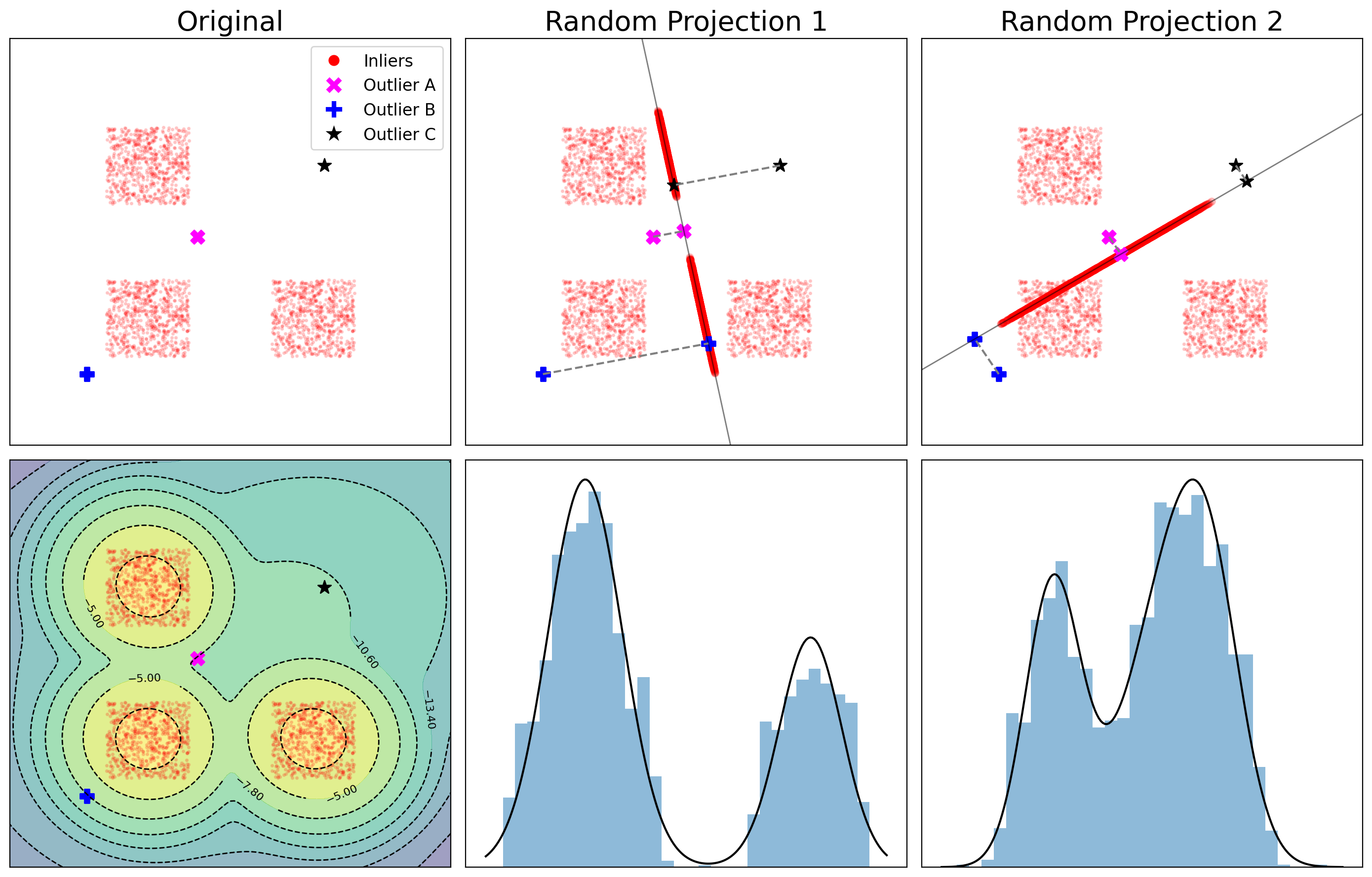
Figure 1: Random projections of two-dimensional data onto one-dimension. In the upper panels, outlier A becomes evident through the first random projection (middle), while outliers B and C are captured using the second random projection axis (right). In the lower panels, the original two-dimensional data exhibit a significant bias when modeled with Gaussian mixtures (left). The one-dimensional projected datasets are shown to be more suitable for Gaussian mixture modeling.

To demonstrate the advantages of subspace outlier ensembles, Figure 1 displays a simulated two-dimensional dataset projected onto one-dimensional random rotation axes. (As clarified below, our proposed method performs dimension reduction only when $p\geq 3$. The provided toy example serves solely as a graphical illustration to emphasize the effectiveness of the subspace ensemble.) The figure illustrates how different random projections reveal each of the three outliers. As a result, by utilizing an ensemble of one-dimensional random projections, all three outliers can be effectively detected. The figure also highlights the benefits of random projection within the Gaussian mixture framework. The original two-dimensional dataset consists of three major clusters uniformly generated on the squares, which clearly deviate from Gaussian distributions. Fitting such data in the original dimension results in a significant bias as shown in the figure. In contrast, the one-dimensional random projections make the projected data more suitable for Gaussian modeling with a few mixture components. This example highlights the efficacy of subspace outlier ensembles in identifying outliers that might remain concealed in a single projection or a full-dimensional analysis.

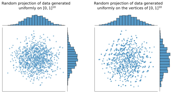
Figure 2: Two-dimensional random projections of ten-dimensional non-Gaussian data of size $1000$. The left panel shows a random projection of data generated uniformly on the unit cube $[0,1]^{10}$, say $\mathbf{x}_{i}\sim\prod_{i=1}^{10}\text{Uniform}(0,1)$, $i=1,\dots,1000$. The right panel shows a random projection of data generated uniformly on the vertices of the unit cube $[0,1]^{10}$, say $\mathbf{x}_{i}\sim\prod_{i=1}^{10}\text{Bernoulli}(1/2)$, $i=1,\dots,1000$.

Figure 2 provides additional clarity on the effectiveness of random projection in conjunction with Gaussian mixture modeling for non-Gaussian original data. The left panel illustrates a two-dimensional random projection of ten-dimensional data randomly generated on the unit cube $[0,1]^{10}$. Despite the non-Gaussian nature of the original data in ten dimensions, the projected data closely resemble two-dimensional Gaussian data. On the right panel, we observe a two-dimensional random projection of ten-dimensional data randomly generated on the vertices of the unit cube $[0,1]^{10}$. In this scenario, the original data are not only non-Gaussian but even discrete with $2^{10}$ possible values rather than continuous. Similar to the first case, the projected data appear well-suited for Gaussian modeling. This observation suggests that utilizing Gaussian mixture models combined with random projection is suitable even for discrete datasets.

In this vein, the original training data $\mathbf{D}\in\mathbb{R}^{N\times p}$ can be projected onto subspaces of dimension smaller than $p$ to generate multiple ensemble components. However, determining the most appropriate dimensionality of subspaces remains unclear. Insufficient dimensionality may fail to capture the overall characteristics of data, while excessive dimensionality may undermine the advantages of subspace ensembles. One common strategy is to choose the subspace dimension as a random integer between $\min\{p,2+\sqrt{p}/2\}$ and $\min\{p,2+\sqrt{p}\}$. (Accordingly, dimension reduction occurs only when $p\geq 3$.) This strategy is based on Aggarwal and Sathe (2015), which suggests that the informative dimensionality of most real-world datasets is not typically larger than $\sqrt{p}$. This range selection ensures a reasonable and effective subspace dimension that aligns with the characteristics of data.

2.2.2 Subsampling Ensembles

Another useful approach for outlier ensembles is subsampling, where instances are randomly drawn from the data without replacement, generating weakly relevant training data for each component of the ensemble. Subsampling, in this context, produces a set of subsamples as ensemble components. The idea is related to bagging (Breiman, 1996), although bagging relies on bootstrap samples generated by sampling with replacement. The application of subsampling in outlier ensembles was initially prominent in the context of the isolation forest (Liu et al., 2008), contributing to improved computational efficiency. Moreover, subsampling has shown to be effective in improving outlier detection accuracy in proximity-based outlier detection methods, such as local outlier factors and nearest neighbors (Zimek et al., 2013; Aggarwal and Sathe, 2015). However, the extent to which subsampling can benefit outlier detection with mixture modeling remains a topic that requires further investigation. In this context, we explore the benefits of employing subsampling for mixture models in outlier detection.

As previously mentioned, the primary bottleneck in employing mixture models for outlier detection lies in their computational costs. To elaborate, training mixture models involves assigning instances to cluster memberships. This procedure is time-consuming and scales with the number of instances, as every data point requires membership determination in the training procedure. For example, in the case of DPGM with MCMC, the membership indicators of all instances must be updated in every iteration of MCMC. Although we utilize variational inference for DPGM to enhance computational efficiency, the challenge persists as an optimization task for membership indicators of all instances. Given that determining the cluster memberships is the most resource-intensive computation, the overal computation time is roughly proportional to the number of instances in the training data, making it challenging to handle large datasets for mixture models in outlier detection. Subsampling is highly effective in reducing computation time in this respect, as the procedure accelerates proportionally with the number of instances in a subsample, thereby reducing overall computation time.

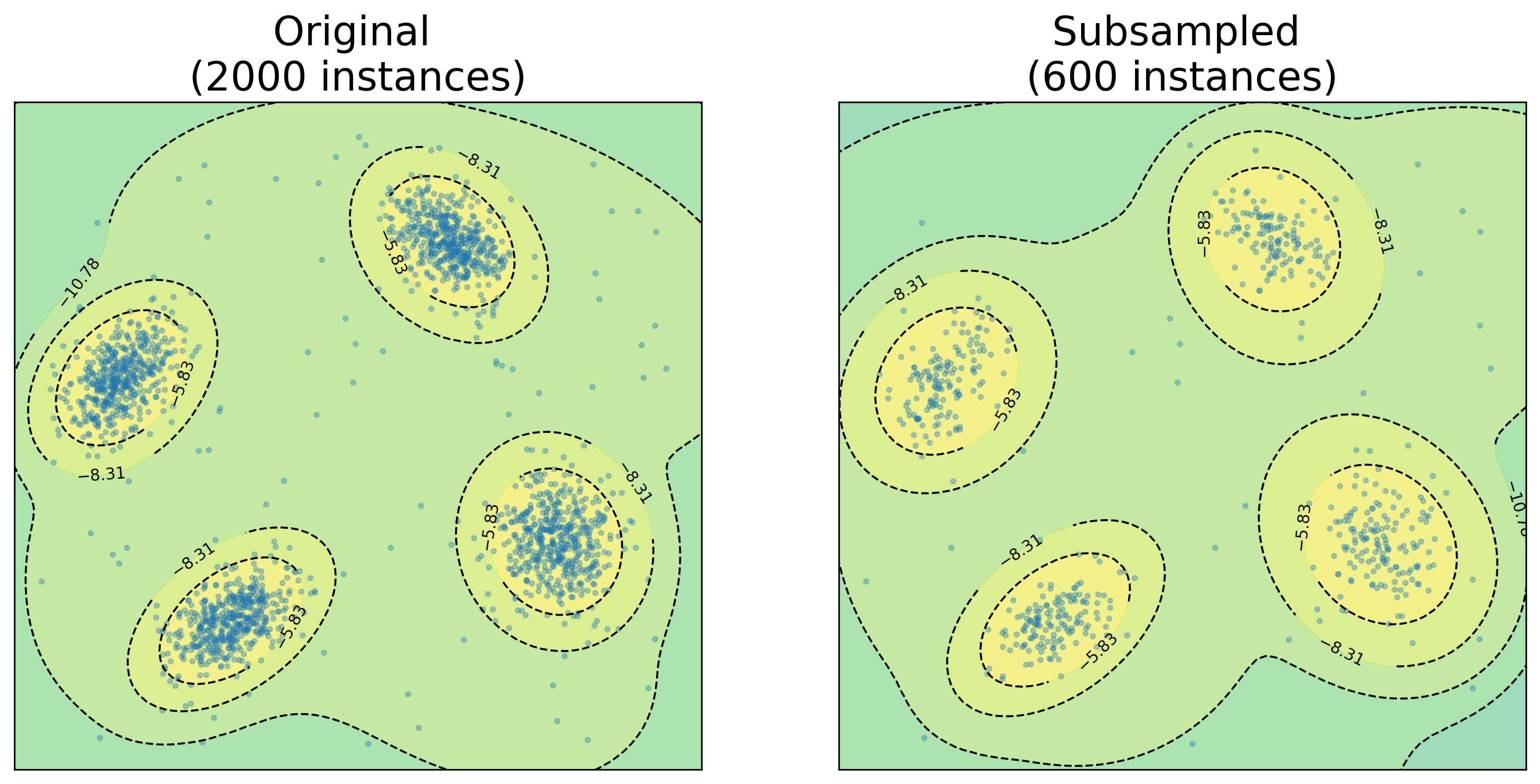
Figure 3: Log-densities estimated by DPGM for the original data (left) and the subsampled data (right). The patterns of the original data are well captured by the subsample.

While achieving significant computational benefits, it is noteworthy that subsampling does not compromise outlier detection accuracy when employing DPGM. Figure 3 illustrates the log-densities of both the original and subsampled data estimated by DPGM. The original dataset consists of four main clusters, interspersed with several outliers throughout. The two estimated densities look sufficiently close, meaning that we can successfully identify the patterns of the original data using the subsampling dataset. Consequently, subsampling proves extremely useful in significantly reducing computation time while maintaining the detection accuracy of the detector.

The training dataset $\mathbf{D}\in\mathbb{R}^{N\times p}$ may consist of a considerable number of instances ($N$), and as such, subsampling can be employed to enhance computational efficiency. However, similar to subspace ensembles, the optimal size of subsamples is still unknown. A natural solution is to introduce variability in the subsample size for each ensemble component. Following Aggarwal and Sathe (2015), we randomly choose the subsample sizes with proportions that range between $\min\{1,50/N\}$ and $\min\{1,1000/N\}$ (although this strategy is referred to as ‘variable subsampling’ in Aggarwal and Sathe (2015), we use the term ‘subsampling’ throughout the paper). It is worth noting that the strategy always generates subsample with sizes between 50 and 1000 as long as the original data size is larger than 1000, meaning that the resulting subsample sizes are not proportional to the original data size. At first glance, this may appear as if the approach does not leverage larger data sizes. However, as pointed out by Aggarwal and Sathe (2015), this is not the case, as a subsample of size 1000 is typically sufficient to model the underlying distribution of the original data. Indeed, the idea performs well even with large original datasets, as an ensemble of small subsamples reduces correlation between ensemble components, thereby enhancing the benefits of the ensemble idea. Our experience in DP mixture modeling for outlier detection aligns with a similar conclusion.

3 Outlier Ensemble of Dirichlet Process Mixtures

This section describes the ensemble-based characteristics of the proposed method, referred to as the outlier ensemble of Dirichlet process mixtures (OEDPM), highlighting its unique properties and considerations for the outlier detection task. The proposed outlier detection algorithm operates through the following three-step process for each ensemble component. First, it estimates the density function of subsampled data within a random subspace using DPGM coupled with mean-field variational inference. Second, it reduces the influence of outliers in density estimation by discarding mixture components with insignificant posterior mixture weights. Third, we calculate the likelihood values of individual instances by evaluating the estimated density function at each respective data point. Subsequently, outlier scores for individual instances are obtained by aggregating likelihood values across all ensemble components. These three procedural steps are elaborated in Sections 3.1, 3.2, and 3.3 respectively. Figure 4 provides an illustrative example demonstrating the procedural sequence.

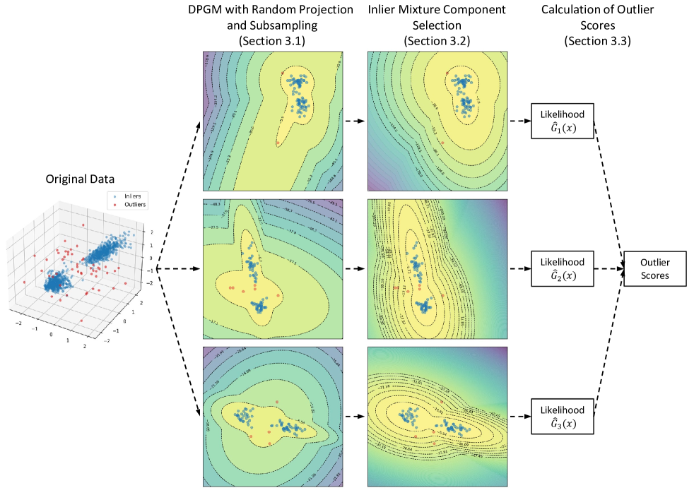
Figure 4: Graphical illustration of OEDPM. The three-dimensional original dataset is fitted by variational DPGM using random projection and subsampling (see Section 3.1). Mixture components with small weights are excluded to better counteract the influence of outliers in constructing outlier detectors (see Section 3.2). Upon pruning the mixture components, outlier scores are obtained using the likelihood (see Section 3.3).

3.1 DPGM with Random Projection and Subsampling

Based on the grounds discussed in Section 2.2, our proposed OEDPM takes full advantage of the benefits of the outlier ensembles by combining random projection and subsampling techniques. The resulting dataset, which is both subsampled and projected, is then trained using DPGM with variational inference. By repeating this process, we obtain $M$ ensemble components that are subsequently combined to determine whether each instance in the full dataset is an outlier or not. To obtain the $m$th ensemble component, $m=1,\dots,M$, from the original dataset $\mathbf{D}\in\mathbb{R}^{N\times p}$ consisting of $N$ instances and $p$ features, the procedure is summarized as follows.

1. For $s_{m}$ drawn from $\text{Uniform}(\min\{1,50/N\},\min\{1,1000/N\})$, randomly draw $n_{m}=\lceil s_{m}N\rceil$ instances without replacement from $\mathbf{D}$ to form a reduced dataset $\mathbf{D}_{m}\in\mathbb{R}^{n_{m}\times p}$.

2. For $d_{m}$ chosen as a random integer between $\min\{p,2+\sqrt{p}/2\}$ and $\min\{p,2+\sqrt{p}\}$, generate a random projection matrix $\mathbf{R}_{m}\in\mathbb{R}^{p\times d_{m}}$, where each element is sampled randomly from $\text{Uniform}(-1,1)$ and the columns are orthogonalized by the Gram-Schmidt process.

3. Produce $\mathbf{X}_{m}=\mathbf{D}_{m}\mathbf{R}_{m}\in\mathbb{R}^{n_{m}\times d_{m}}$ to generate a reduced dataset projected onto a random subspace.

4. Fit DPGM to $\mathbf{X}_{m}$ using the mean-field variational inference.

Our method places great emphasis on computational feasibility while mitigating the risk of overfitting that may arise when using a single original dataset. This ensemble approach has been shown to reduce variance by capitalizing on the diversity of base detectors (Aggarwal and Sathe, 2015). Furthermore, the reduced dimensionality and size of the training data lead to substantial computational savings, effectively addressing our concerns regarding probabilistic mixture models.

3.2 Inlier Mixture Component Selection

The fundamental principle of outlier detection involves investigating the normal patterns within a dataset. The success of an outlier detection task depends on how well the method can model the inlier instances to identify outlying points that deviate from normal instances. However, in unsupervised outlier detection problems, we deal with contaminated datasets where normal instances are mixed with noise and potential outliers (Hodge and Austin, 2004). An effective algorithm should be capable of filtering out outliers during training. Regarding this, the advantage of DPGM in automatically determining the optimal number of mixture components can also be problematic, potentially leading to overfitting of anomaly instances. To address this potential issue, we include pruning of irrelevant mixture components based on the posterior information of the mixture weights of DPGM.

Among the limited recognized characteristics of outliers, it is evident that outliers are isolated instances that tend to deviate from the majority of data points. Hence, a natural assumption is that outliers will not conform to any of the existing cluster memberships, resulting in less stable clusters that contain fewer instances. For ensemble component $m\in\{1,\dots,M\}$, let $\hat{K}_{m}\leq K$ be the number of mixture components determined by DPGM and $\{\hat{\pi}_{mk}\}_{k=1}^{\hat{K}_{m}}$ be the estimated mixture weights. We discard mixture component $k\in\{1,\dots,\hat{K}_{m}\}$ if $\hat{\pi}_{mk}<1/\hat{K}_{m}$. (If there is no mixture component with $\hat{\pi}_{mk}\geq 1/\hat{K}_{m}$, only the component with the largest $\hat{\pi}_{mk}$ is chosen.) As a result, we can obtain a more robust mixture distribution comprising solely of inlier Gaussian components, effectively eliminating outliers from the inlier set. This process is applied to all ensemble components for $m=1,\dots,M$. Our experience indicates that selecting inlier mixture components is crucial for achieving reasonable performance in OEDPM. The advantages of this pruning step are clearly illustrated in Figure 4.

3.3 Calculation of Outlier Scores

DPGM is commonly acknowledged as a probabilistic clustering method, with each identified cluster potentially serving as a criterion for outlier detection (Shotwell and Slate, 2011). Specifically, from a clustering perspective, instances that do not align with the predominant clusters can be characterized as outliers (Yu et al., 2002). However, using cluster memberships for identifying outliers may not be advisable, as DPGM offers a global characteristic of the entire dataset through the likelihood, which stands in contrast to proximity-based clustering algorithms. Therefore, it is more appropriate to compute outlier scores based on the likelihood rather than relying solely on the cluster memberships.

Given the trained $m$th ensemble component, the likelihood of an instance $\mathbf{x}\in\mathbb{R}^{d_{m}}$ is expressed as

$$\hat{G}_{m}(\mathbf{x})=\sum_{k=1}^{\hat{K}_{m}^{\ast}}\hat{\pi}_{mk}^{\ast}{\text{N}}_{d_{m}}(\mathbf{x};\hat{\boldsymbol{\mu}}_{mk},\hat{\boldsymbol{\Sigma}}_{mk}),$$

where $\hat{K}_{m}^{\ast}$ is the number of mixture components after the pruning described in Section 3.2, $\hat{\pi}_{mk}^{\ast}$ is the weight renormalized such that $\sum_{k=1}^{\hat{K}_{m}^{\ast}}\hat{\pi}_{mk}^{\ast}=1$ with the pruned mixture components, and $\hat{\boldsymbol{\mu}}_{mk}$ and $\hat{\boldsymbol{\Sigma}}_{mk}$ are the parameters fitted by the mean-field variational inference for DPGM. A relatively small likelihood value of an instance suggests it could potentially be an outlier. To define the outlier score, we need to consider a threshold that assigns a binary score to a test instance within a reduced subspace. We examine the following two methods of obtaining this threshold.

• A contamination parameter $\phi\in(0,1)$ can be used in constructing the outlier scores. This construction is particularly useful if the proportion of outliers in the dataset is roughly known to us. For a given $\phi\in(0,1)$, we define the cut-off threshold $T_{m}$ as the $100\phi\%$ quantile of $\log G(\mathbf{x}_{m1}),\dots,\log G(\mathbf{x}_{mn_{m}})$, where $\mathbf{x}_{mi}$ is the $i$th row (instance) of $\mathbf{X}_{m}$.

• It is also feasible to establish a threshold without a contamination parameter. This approach may be beneficial when the proportion of outliers is entirely unknown to us. Specifically, we define the cut-off threshold $T_{m}$ as $T_{m}=\text{Q1}_{m}-1.5\times\text{IQR}_{m}$ using the rule of thumb, where $\text{Q1}_{m}$ and $\text{IQR}_{m}$ are the first quartile and the interquartile range (IQR) of $\log G(\mathbf{x}_{m1}),\dots,\log G(\mathbf{x}_{mn_{m}})$, respectively.

Let $\mathbf{D}^{\text{test}}\in\mathbb{R}^{N^{\text{test}}\times p}$ represent a test dataset. This dataset can coinside with the original dataset $\mathbf{D}$, as our interest lies on identifying outliers within the provided data, or it can consist of entirely new data collected separately. Using the random projection matrices $\mathbf{R}_{m}\in\mathbb{R}^{p\times d_{m}}$, $m=1,\dots,M$, used for training, the test instances projected onto the subspaces are expressed by $\mathbf{X}_{m}^{\text{test}}=\mathbf{D}^{\text{test}}\mathbf{R}_{m}\in\mathbb{R}^{N^{\text{test}}\times d_{m}}$, $m=1,\dots,M$. With the threshold $T_{m}$ defined in either way, we calculate the outlier score of each test instance using binary thresholding according to their likelihood values,

$$O_{i}=\frac{1}{M}\sum_{m=1}^{M}\mathbbm{1}\{\log\hat{G}_{m}(\mathbf{x}^{\text{test}}_{mi})<T_{m}\},\quad i=1,\dots,N^{\text{test}},$$ (4)

where $\mathbf{x}^{\text{test}}_{mi}$ is the $i$th row of $\mathbf{X}_{m}^{\text{test}}$. A voting classifier categorizes $\mathbf{x}^{\text{test}}_{mi}$ as an outlier if $O_{i}>1/2$ and as an inlier otherwise. Even when a specific contamination parameter $\phi\in(0,1)$ is used to determine the thresholds $T_{m}$, the resulting estimate of the outlier proportion is not necessarily identical to $\phi$ because the identified outliers are determined by the rule $O_{i}>1/2$ averaging over all ensemble components. This introduces some degree of robustness against the specification of $\phi$.

Additionally, instead of the binary thresholding $\mathbbm{1}\{\log\hat{G}_{m}(\mathbf{x}^{\text{test}}_{mi})<T_{m}\}$ used in (4), one might also define the outlier score directly using the magnitude of the likelihood values, for example, $T_{m}-\log\hat{G}_{m}(\mathbf{x}^{\text{test}}_{mi})$. However, our observation reveals that using the binary thresholding significantly improves the stability and robustness of our outlier detection task.

4 Numerical Results

4.1 Sensitivity Analysis

We evaluate the performance of OEDPM using the benchmark datasets included in the ODDS library (https://odds.cs.stonybrook.edu), where 27 multi-dimensional point datasets are available with outlier labels. (While the ODDS library seemingly contains 31 such datasets, four of these datasets are unavailable due to their incompleteness.) The datasets are categorized as either continuous or discrete based on the nature of the values of instances, with a few presented in a mixed form. The details of the benchmark datasets are summarized in Table 1.

Dataset	Size ($N$)	Dimension ($p$)	# of outliers ($\%$)	Type
Smtp (KDDCUP99)	95156	3	30 $(0.03\%)$	Continuous
Http (KDDCUP99)	567479	3	2211 $(0.39\%)$	Continuous
ForestCover	286048	10	2747 $(0.96\%)$	Continuous
Satimage	5803	36	71 $(1.22\%)$	Continuous
Speech	3686	400	61 $(1.65\%)$	Continuous
Pendigits	6870	16	156 $(2.27\%)$	Continuous
Mammography	11183	6	260 $(2.32\%)$	Continuous
Thyroid	3772	6	93 $(2.47\%)$	Continuous
Optdigits	5216	64	150 $(2.88\%)$	Continuous
Musk	3062	166	97 $(3.17\%)$	Mixed
Vowels	1456	12	50 $(3.43\%)$	Continuous
Lympho	148	18	6 $(4.05\%)$	Discrete
Glass	214	9	9 $(4.21\%)$	Continuous
WBC	378	30	21 $(5.56\%)$	Continuous
Letter Recognition	1600	32	100 $(6.25\%)$	Continuous
Shuttle	49097	9	3511 $(7.15\%)$	Mixed
Annthyroid	7200	6	534 $(7.42\%)$	Continuous
Wine	129	13	10 $(7.75\%)$	Continuous
Mnist	7603	100	700 $(9.21\%)$	Continuous
Cardio	1831	21	176 $(9.61\%)$	Continuous
Vertebral	240	6	30 $(12.50\%)$	Continuous
Arrhythmia	452	274	66 $(14.60\%)$	Mixed
Heart	267	44	55 $(20.60\%)$	Continuous
Satellite	6435	36	2036 $(31.64\%)$	Continuous
Pima	768	8	268 $(34.90\%)$	Mixed
BreastW	683	9	239 $(34.99\%)$	Discrete
Ionosphere	351	33	126 $(35.90\%)$	Mixed

Table 1: Details of the 27 benchmark datasets, sorted in ascending order based on the proportion of outliers. The dataset type is labeled as ‘Continuous’ when all features are continuous, ‘Discrete’ when all features are discrete, and ‘Mixed’ otherwise.

To examine the sensitivity of the contamination parameter $\phi$, we apply OEDPM to each benchmark dataset with various values $\phi$. For this numerical study, the test dataset is chosen to be identical to the training dataset. Each specific value of $\phi$ produces outlier scores $O_{i}$ for every instance, classifying instances as outliers if their corresponding $O_{i}$ are greater than $1/2$. Subsequently, we compute the precision, recall, and F1-score based on the obtained outlier detection results. We also obtain the F1-score using the strategy with the IQR outlined in Section 3.3.

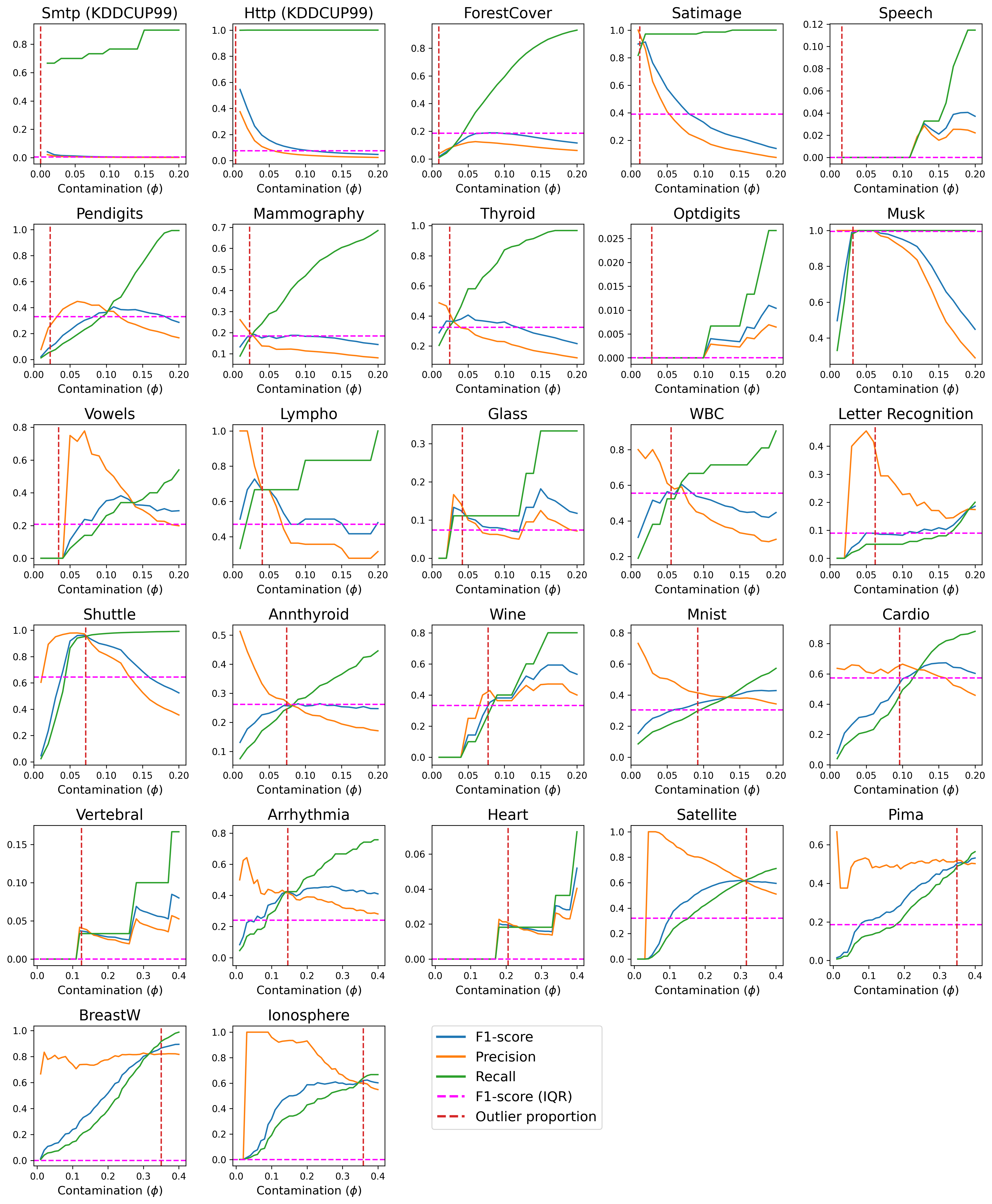
Figure 5: Sensitivity analysis for the contamination parameter $\phi$ using the 27 benchmark datasets.

The results are illustrated in Figure 5. Overall, the performance appears satisfactory when $\phi$ is chosen close to the true outlier proportion for each dataset. This implies that, although the estimated proportion of outliers is not necessarily identical to a given value of $\phi$, matching $\phi$ closely with the true outlier proportion is a reasonable idea. Unfortunately, the outlier proportion is generally unknown to us. Using the IQR is often satisfactory. However, this sometimes results in very poor performance with zero F1-scores. Instead, it is evident that using a fixed value of $\phi$ near $0.1$ outperforms using the IQR, regardless of the outlier proportion in most cases (compare the blue solid and pink dashed lines). Therefore, we use the contamination parameter with $\phi=0.1$ as the default value instead of using the IQR to calculate the outlier scores.

4.2 Comparison with Other Methods

We now compare OEDPM with other competitors for unsupervised outlier detection available in the Python toolbox PyOD (Zhao et al., 2019). We consider 15 methods ranging from classical to state-of-the-art methodologies. These include nearly all the methods available in PyOD for outlier detection of point datasets. The competing methods are summarized in Table 2. The abbreviations in Table 2 are used for Table LABEL:tab:benchmark below.

Method	Literature	Category
Local Outlier Factor (LOF)	Breunig et al. (2000)	Proximity-Based
K-Nearest neighbors (KNN)	Ramaswamy et al. (2000)	Proximity-Based
One-Class Support Vector Machines (OCSVM)	Schölkopf et al. (2001)	Probabilistic
Principal Component Analysis (PCA)	Shyu et al. (2003)	Probabilistic
Angle-Based Outlier Detector (ABOD)	Kriegel et al. (2008)	Probabilistic
Isolation Forest (IF)	Liu et al. (2008)	Outlier Ensembles
Variational Autoencoder (VAE)	Kingma and Welling (2013)	Neural Networks
Autoencoder (AE)	Sakurada and Yairi (2014)	Neural Networks
Lightweight Online Detector of Anomalies (LODA)	Pevnỳ (2016)	Outlier Ensembles
Isolation using Nearest-Neighbor Ensembles (INNE)	Bandaragoda et al. (2018)	Outlier Ensembles
Deep One-Class Classification (DSVDD)	Ruff et al. (2018)	Neural Networks
Rotation-Based Outlier Detection (ROD)	Almardeny et al. (2020)	Proximity-Based
Copula-Based Outlier Detection (COPOD)	Li et al. (2020)	Probabilistic
Empirical CDF-Based Outlier Detection (ECOD)	Li et al. (2022)	Probabilistic
Deep Isolation Forest (DIF)	Xu et al. (2023)	Outlier Ensembles

Table 2: Details of the 15 competing methods sorted in chronological order.

All competing methods and OEDPM are applied to detect outliers in the 27 benchmark datasets listed in Table 1. For a fair comparison, we set the contamination to $0.1$ for all methods including OEDPM. For each method, we calculate the F1-scores of outlier detection for the benchmark datasets, and the results are provided in Table LABEL:tab:benchmark. The findings suggest that recent methods generally exhibit better performance than classical methods in outlier detection. Among such state-of-the-art methods, our proposed OEDPM performs reasonably well and outperforms other competitors in terms of F1-scores. Specifically, OEDPM emerges as the winner in competitions for five benchmark datasets, whereas other competitors do not achieve as many wins in the competitions. Even when OEDPM does not secure the first position, its F1-scores generally remain competitive compared to other participants. Furthermore, the last row of Table 1 illustrates the average F1-scores across all benchmark datasets. It is clear that OEDPM demonstrates the highest average F1-score, affirming its superior performance among the methods considered in our numerical study.

5 Discussion

In this study, we introduced OEDPM for unsupervised outlier detection. By incorporating two outlier ensemble ideas for DPGM with variational inference, the proposed OEDPM offers unique characteristics that are not achieved by traditional Gaussian mixture modeling. Specifically, the subspace ensemble with random projection enables efficient data characterization through dimension reduction, rendering data suitable for Gaussian modeling even in cases where they deviate significantly from Gaussian distributions. The subsampling ensemble effectively addresses the challenge of long computation time, which is one of the most significant issues in dealing with the mixture modeling framework, without compromising detection accuracy. Our numerical study validates the performance of OEDPM.

One key factor contributing to the success of the proposed method is the outlier ensemble with random projection, which is characterized by linear projection onto smaller subspaces. While the linearity contributes to simplicity and robustness, it may be seen as a constraint in the modeling process. An alternative approach could involve considering nonlinear projection to construct outlier ensembles. We intend to investigate this direction in future research.

References

- Aggarwal (2013) Aggarwal, C. C. (2013). Outlier ensembles: position paper. ACM SIGKDD Explorations Newsletter 14(2), 49–58.
- Aggarwal (2017) Aggarwal, C. C. (2017). Outlier Analysis (Second ed.). Springer.
- Aggarwal et al. (2001) Aggarwal, C. C., A. Hinneburg, and D. A. Keim (2001). On the surprising behavior of distance metrics in high dimensional space. In Proceedings of the International Conference on Database Theory, pp. 420–434.
- Aggarwal and Sathe (2015) Aggarwal, C. C. and S. Sathe (2015). Theoretical foundations and algorithms for outlier ensembles. ACM SIGKDD Explorations Newsletter 17(1), 24–47.
- Aggarwal and Yu (2001) Aggarwal, C. C. and P. S. Yu (2001). Outlier detection for high dimensional data. In Proceedings of the 2001 ACM SIGMOD International Conference on Management of Data, pp. 37–46.
- Aldous et al. (1985) Aldous, D. J., I. A. Ibragimov, J. Jacod, and D. J. Aldous (1985). Exchangeability and Related Topics. Springer.
- Almardeny et al. (2020) Almardeny, Y., N. Boujnah, and F. Cleary (2020). A novel outlier detection method for multivariate data. IEEE Transactions on Knowledge and Data Engineering 34(9), 4052–4062.
- Arisoy and Kayabol (2021) Arisoy, S. and K. Kayabol (2021). Nonparametric Bayesian background estimation for hyperspectral anomaly detection. Digital Signal Processing 111, 102993.
- Bahrololum and Khaleghi (2008) Bahrololum, M. and M. Khaleghi (2008). Anomaly intrusion detection system using Gaussian mixture model. In Proceedings of the 3rd International Conference on Convergence and Hybrid Information Technology, pp. 1162–1167.
- Bandaragoda et al. (2018) Bandaragoda, T. R., K. M. Ting, D. Albrecht, F. T. Liu, Y. Zhu, and J. R. Wells (2018). Isolation-based anomaly detection using nearest-neighbor ensembles. Computational Intelligence 34(4), 968–998.
- Bingham and Mannila (2001) Bingham, E. and H. Mannila (2001). Random projection in dimensionality reduction: applications to image and text data. In Proceedings of the 7th ACM SIGKDD International Conference on Knowledge Discovery and Data Mining, pp. 245–250.
- Bishop and Nasrabadi (2006) Bishop, C. M. and N. M. Nasrabadi (2006). Pattern Recognition and Machine Learning. Springer.
- Blackwell and MacQueen (1973) Blackwell, D. and J. B. MacQueen (1973). Ferguson distributions via Pólya urn schemes. The Annals of Statistics 1(2), 353–355.
- Blei and Jordan (2006) Blei, D. M. and M. I. Jordan (2006). Variational inference for Dirichlet process mixtures. Bayesian Analysis 1(1), 121–143.
- Blei et al. (2017) Blei, D. M., A. Kucukelbir, and J. D. McAuliffe (2017). Variational inference: A review for statisticians. Journal of the American Statistical Association 112(518), 859–877.
- Bradley et al. (2000) Bradley, P. S., U. Fayyad, and C. Reina (2000). Clustering very large databases using EM mixture models. In Proceedings of the 15th International Conference on Pattern Recognition, pp. 76–80.
- Breiman (1996) Breiman, L. (1996). Bagging predictors. Machine Learning 24(2), 123–140.
- Breiman (2001) Breiman, L. (2001). Random forests. Machine Learning 45(1), 5–32.
- Breunig et al. (2000) Breunig, M. M., H.-P. Kriegel, R. T. Ng, and J. Sander (2000). LOF: identifying density-based local outliers. In Proceedings of the ACM SIGMOD International Conference on Management of Data, pp. 93–104.
- Chen et al. (2001) Chen, Y., X. S. Zhou, and T. S. Huang (2001). One-class SVM for learning in image retrieval. In Proceedings of the International Conference on Image Processing, pp. 34–37.
- Diaconis and Freedman (1984) Diaconis, P. and D. Freedman (1984). Asymptotics of graphical projection pursuit. The Annals of Statistics 12(3), 793–815.
- Emmott et al. (2013) Emmott, A. F., S. Das, T. Dietterich, A. Fern, and W.-K. Wong (2013). Systematic construction of anomaly detection benchmarks from real data. In Proceedings of the 19th ACM SIGKDD Workshop on Outlier Detection and Description, pp. 16–21.
- Ferguson (1973) Ferguson, T. S. (1973). A Bayesian analysis of some nonparametric problems. The Annals of Statistics 1(2), 209–230.
- Friedman (1987) Friedman, J. H. (1987). Exploratory projection pursuit. Journal of the American Statistical Association 82(397), 249–266.
- Gelman et al. (1995) Gelman, A., J. B. Carlin, H. S. Stern, and D. B. Rubin (1995). Bayesian Data Analysis. Chapman and Hall/CRC.
- Ghahramani and Beal (2000) Ghahramani, Z. and M. Beal (2000). Propagation algorithms for variational Bayesian learning. Advances in Neural Information Processing Systems, 507–513.
- Grubbs (1969) Grubbs, F. E. (1969). Procedures for detecting outlying observations in samples. Technometrics 11(1), 1–21.
- Hautamaki et al. (2004) Hautamaki, V., I. Karkkainen, and P. Franti (2004). Outlier detection using k-nearest neighbor graph. In Proceedings of the 17th International Conference on Pattern Recognition, pp. 430–433.
- Hawkins et al. (2002) Hawkins, S., H. He, G. Williams, and R. Baxter (2002). Outlier detection using replicator neural networks. In International Conference on Data Warehousing and Knowledge Discovery, pp. 170–180. Springer.
- Hodge and Austin (2004) Hodge, V. and J. Austin (2004). A survey of outlier detection methodologies. Artificial Intelligence Review 22(2), 85–126.
- Ishwaran and James (2001) Ishwaran, H. and L. F. James (2001). Gibbs sampling methods for stick-breaking priors. Journal of the American Statistical Association 96(453), 161–173.
- Jain and Neal (2004) Jain, S. and R. M. Neal (2004). A split-merge Markov chain Monte Carlo procedure for the Dirichlet process mixture model. Journal of Computational and Graphical Statistics 13(1), 158–182.
- Jordan et al. (1999) Jordan, M. I., Z. Ghahramani, T. S. Jaakkola, and L. K. Saul (1999). An introduction to variational methods for graphical models. Machine Learning 37, 183–233.
- Kaltsa et al. (2018) Kaltsa, V., A. Briassouli, I. Kompatsiaris, and M. G. Strintzis (2018). Multiple hierarchical Dirichlet processes for anomaly detection in traffic. Computer Vision and Image Understanding 169, 28–39.
- Keller et al. (2012) Keller, F., E. Müller, and K. Bohm (2012). HiCS: High contrast subspaces for density-based outlier ranking. In Proceedings of the 28th IEEE International Conference on Data Engineering, pp. 1037–1048.
- Kingma and Welling (2013) Kingma, D. P. and M. Welling (2013). Auto-encoding variational Bayes. arXiv preprint arXiv:1312.6114.
- Knox and Ng (1998) Knox, E. M. and R. T. Ng (1998). Algorithms for mining distance-based outliers in large datasets. In Proceedings of the International Conference on Very Large Data Bases, pp. 392–403.
- Kriegel et al. (2009) Kriegel, H.-P., P. Kröger, E. Schubert, and A. Zimek (2009). Outlier detection in axis-parallel subspaces of high dimensional data. In Proceedings of the Pacific-Asia Conference on Knowledge Discovery and Data Mining, pp. 831–838.
- Kriegel et al. (2008) Kriegel, H.-P., M. Schubert, and A. Zimek (2008). Angle-based outlier detection in high-dimensional data. In Proceedings of the 14th ACM SIGKDD International Conference on Knowledge Discovery and Data Mining, pp. 444–452.
- Kurihara et al. (2007) Kurihara, K., M. Welling, and Y. W. Teh (2007). Collapsed variational Dirichlet process mixture models. In Proceedings of the International Joint Conference on Artificial Intelligence, pp. 2796–2801.
- Laxhammar et al. (2009) Laxhammar, R., G. Falkman, and E. Sviestins (2009). Anomaly detection in sea traffic-a comparison of the Gaussian mixture model and the kernel density estimator. In Proceedings of the 12th International Conference on Information Fusion, pp. 756–763.
- Lazarevic and Kumar (2005) Lazarevic, A. and V. Kumar (2005). Feature bagging for outlier detection. In Proceedings of the 11th ACM SIGKDD International Conference on Knowledge Discovery and Data Mining, pp. 157–166.
- Li et al. (2016) Li, L., R. J. Hansman, R. Palacios, and R. Welsch (2016). Anomaly detection via a Gaussian mixture model for flight operation and safety monitoring. Transportation Research Part C: Emerging Technologies 64, 45–57.
- Li et al. (2020) Li, Z., Y. Zhao, N. Botta, C. Ionescu, and X. Hu (2020). COPOD: copula-based outlier detection. IEEE International Conference on Data Mining, 1118–1123.
- Li et al. (2022) Li, Z., Y. Zhao, X. Hu, N. Botta, C. Ionescu, and G. Chen (2022). ECOD: Unsupervised outlier detection using empirical cumulative distribution functions. IEEE Transactions on Knowledge and Data Engineering.
- Liu et al. (2008) Liu, F. T., K. M. Ting, and Z.-H. Zhou (2008). Isolation forest. In Proceedings of the 8th IEEE International Conference on Data Mining, pp. 413–422.
- Müller et al. (2011) Müller, E., M. Schiffer, and T. Seidl (2011). Statistical selection of relevant subspace projections for outlier ranking. In Proceedings of the 27th IEEE International Conference on Data Engineering, pp. 434–445.
- Neal (2000) Neal, R. M. (2000). Markov chain sampling methods for Dirichlet process mixture models. Journal of Computational and Graphical Statistics 9(2), 249–265.
- Pevnỳ (2016) Pevnỳ, T. (2016). Loda: Lightweight on-line detector of anomalies. Machine Learning 102, 275–304.
- Ramaswamy et al. (2000) Ramaswamy, S., R. Rastogi, and K. Shim (2000). Efficient algorithms for mining outliers from large data sets. In Proceedings of the International Conference on Management of Data, pp. 427–438.
- Ruff et al. (2018) Ruff, L., R. Vandermeulen, N. Goernitz, L. Deecke, S. A. Siddiqui, A. Binder, E. Müller, and M. Kloft (2018). Deep one-class classification. In International Conference on Machine Learning, pp. 4393–4402.
- Sakurada and Yairi (2014) Sakurada, M. and T. Yairi (2014). Anomaly detection using autoencoders with nonlinear dimensionality reduction. In Proceedings of the 2nd Workshop on Machine Learning for Sensory Data Analysis, pp. 4–11.
- Samé et al. (2007) Samé, A., C. Ambroise, and G. Govaert (2007). An online classification EM algorithm based on the mixture model. Statistics and Computing 17(3), 209–218.
- Schölkopf et al. (2001) Schölkopf, B., J. C. Platt, J. Shawe-Taylor, A. J. Smola, and R. C. Williamson (2001). Estimating the support of a high-dimensional distribution. Neural Computation 13(7), 1443–1471.
- Sethuraman (1994) Sethuraman, J. (1994). A constructive definition of Dirichlet priors. Statistica Sinica, 639–650.
- Shotwell and Slate (2011) Shotwell, M. S. and E. H. Slate (2011). Bayesian outlier detection with Dirichlet process mixtures. Bayesian Analysis 6(4), 665–690.
- Shyu et al. (2003) Shyu, M.-L., S.-C. Chen, K. Sarinnapakorn, and L. Chang (2003). A novel anomaly detection scheme based on principal component classifier. In Proceedings of the IEEE Foundations and New Directions of Data Mining Workshop, pp. 172–179.
- Strehl and Ghosh (2002) Strehl, A. and J. Ghosh (2002). Cluster ensembles—a knowledge reuse framework for combining multiple partitions. Journal of Machine Learning Research 3(Dec), 583–617.
- Thudumu et al. (2020) Thudumu, S., P. Branch, J. Jin, and J. J. Singh (2020). A comprehensive survey of anomaly detection techniques for high dimensional big data. Journal of Big Data 7(1), 1–30.
- Varadarajan et al. (2017) Varadarajan, J., R. Subramanian, N. Ahuja, P. Moulin, and J.-M. Odobez (2017). Active online anomaly detection using Dirichlet process mixture model and Gaussian process classification. In Proceedings of 2017 IEEE Winter Conference on Applications of Computer Vision, pp. 615–623.
- Veracini et al. (2009) Veracini, T., S. Matteoli, M. Diani, and G. Corsini (2009). Fully unsupervised learning of Gaussian mixtures for anomaly detection in hyperspectral imagery. In Proceedings of the 9th International Conference on Intelligent Systems Design and Applications, pp. 596–601.
- Xu et al. (2023) Xu, H., G. Pang, Y. Wang, and Y. Wang (2023). Deep isolation forest for anomaly detection. IEEE Transactions on Knowledge and Data Engineering 35(12), 12591–12604.
- Yang et al. (2009) Yang, X., L. J. Latecki, and D. Pokrajac (2009). Outlier detection with globally optimal exemplar-based GMM. In Proceedings of the 2009 SIAM International Conference on Data Mining, pp. 145–154.
- Yu et al. (2002) Yu, D., G. Sheikholeslami, and A. Zhang (2002). Findout: Finding outliers in very large datasets. Knowledge and Information Systems 4(4), 387–412.
- Zhao et al. (2019) Zhao, Y., Z. Nasrullah, and Z. Li (2019). PyOD: A Python toolbox for scalable outlier detection. Journal of Machine Learning Research 20(96), 1–7.
- Zhou (2012) Zhou, Z.-H. (2012). Ensemble Methods: Foundations and Algorithms. CRC Press.
- Zimek et al. (2013) Zimek, A., M. Gaudet, R. J. Campello, and J. Sander (2013). Subsampling for efficient and effective unsupervised outlier detection ensembles. In Proceedings of the 19th ACM SIGKDD International Conference on Knowledge Discovery and Data Mining, pp. 428–436.