Single production of an exotic vector-like $Y$ quark
at future high energy $pp$ colliders

Abstract

Vector-like quarks have been predicted in various new physics scenarios beyond the Standard Model (SM). In a simplified modelling of a $(B,Y)$ doublet including a vector-like quark $Y$, with charge $-\frac{4}{3}$e, there are only two free parameters: the $Y$ coupling $\kappa_{Y}$ and mass $m_{Y}$. In the five flavor scheme, we investigate the single production of the $Y$ state decaying into $Wb$ at the Large Hadron Collider (LHC) Run-III and High-Luminosity LHC (HL-LHC) operating at $\sqrt{s}$ = 14 TeV, the possible High-Energy LHC (HE-LHC) with $\sqrt{s}$ = 27 TeV as well as the Future Circular Collider in hadron-hadron mode (FCC-hh) with $\sqrt{s}$ = 100 TeV. Through detailed signal-to-background analyses and detector simulations, we assess the exclusion capabilities of the $Y$ state at the different colliders. We find that this can be improved significantly with increasing collision energy, especially at the HE-LHC and FCC-hh, both demonstrating an obvious advantage with respect to the HL-LHC case in the case of high $m_{Y}$. Assuming a 10% systematic uncertainty on the background event rate, the exclusion capabilities are summarized as follows: (1) the LHC Run-III can exclude the correlated regions of $\kappa_{Y}\in[0.044,0.5]$ and $m_{Y}\in[1000\text{ GeV},3099\text{ GeV}]$ with integrated luminosity $L=300\text{ fb}^{-1}$; (2) the HL-LHC can exclude the correlated regions of $\kappa_{Y}\in[0.027,0.5]$ and $m_{Y}\in[1000\text{ GeV},3653\text{ GeV}]$ with $L=3$ ab^-1; (3) the HE-LHC can exclude the correlated regions of $\kappa_{Y}\in[0.030,0.5]$ and $m_{Y}\in[1000\text{ GeV},4936\text{ GeV}]$ with $L=3$ ab^-1; (4) the FCC-hh can exclude the correlated regions of $\kappa_{Y}\in[0.051,0.5]$ and $m_{Y}\in[1000\text{ GeV},6610\text{ GeV}]$ with $L=3$ ab^-1.

I introduction

In 2012, the ATLAS and CMS experiments at the Large Hadron Collider (LHC) made a significant discovery by confirming the existence of the Higgs boson, thereby providing further validation for the Standard Model (SM) ATLAS:2012yve ; CMS:2012qbp . However, the SM has certain limits in addressing several prominent issues, such as neutrino masses, gauge hierarchy, dark matter and dark energy. In various new physics scenarios like little Higgs models Arkani-Hamed:2002ikv ; Han:2003wu ; Chang:2003vs ; Cao:2007pv , extra dimensions 4 , composite Higgs models Agashe:2004rs ; Bellazzini:2014yua ; Low:2015nqa ; Bian:2015ota ; He:2001fz ; He:1999vp and other extended models 6 ; 7 ; 8 , Vector-Like Quarks (VLQs) are predicted to play a role in resolving the gauge hierarchy problem by mitigating the quadratic divergences of the Higgs field. Such VLQs are fermions with spin $\frac{1}{2}$ and possess the unique characteristic of undergoing both left- and right-handed component transformations under the Electro-Weak (EW) symmetry group of the SM 9 . Unlike chiral quarks, VLQs do not acquire masses through Yukawa couplings to the Higgs field and therefore have the potential to counterbalance loop corrections to the Higgs boson mass stemming from the top quark of the SM. Furthermore, VLQs can generate characteristic signatures at colliders and have been widely studied (see, for example, Banerjee:2023upj ; Benbrik:2023xlo ; Zeng:2023ljl ; Canbay:2023vmj ; Belyaev:2023yym ; Shang:2023ebe ; Yang:2023wnv ; Bhardwaj:2022nko ; Bhardwaj:2022wfz ; Bardhan:2022sif ; Shang:2022tkr ; Freitas:2022cno ; Benbrik:2022kpo ; Corcella:2021mdl ; VLX2021 ; Belyaev:2021zgq ; Deandrea:2021vje ; Dasgupta:2021fzw ; King:2020mau ; Liu:2019jgp ; Benbrik:2019zdp ; Xie:2019gya ; Bizot:2018tds ; Cacciapaglia:2018qep ; Cacciapaglia:2018lld ; Carvalho:2018jkq ; CMS:2018kcw ; Barducci:2017xtw ; CMS:2017voh ; Chen:2016yfv ; Arhrib:2016rlj ; Cacciapaglia:2015ixa ; Angelescu:2015kga ; Panizzi:2014dwa ; Panizzi:2014tya ; Cacciapaglia:2012dd ; Okada:2012gy ; Cacciapaglia:2011fx ; delAguila:1989rq ).

A VLQ model typically introduces four new states: $T$, $B$, $X$ and $Y$, their electric charges being $+\frac{2}{3}$, $-\frac{1}{3}$, $+\frac{5}{3}$ and $-\frac{4}{3}$, respectively. In such kind of model, VLQs can be categorized into three types: singlets $(T)$, $(B)$, doublets $(X,T)$, $(T,B)$, $(B,Y)$ and triplets $(X,T,B)$, $(T,B,Y)$. Notably, the $Y$ quark cannot exist as a singlet. Further, it is expected to decay with a 100% Branching Ratio (BR) into a $b$ quark and $W$ boson when $Y$ is lighter than the other VLQs, whether in a doublet or triplet.

In this study, we will focus on the observability of single $Y$ production at the Large Hadron Collider (LHC) Run-III, the High-Luminosity LHC (HL-LHC) Gianotti:2002xx ; Apollinari:2017lan , the High-Energy LHC (HE-LHC) FCC:2018bvk and the Future Circular Collider operating in hadron-hadron mode (FCC-hh) FCC:2018vvp , specifically, within the $(B,Y)$ doublet realisation.

The ATLAS Collaboration conducted a search for a VLQ $Y$ at 13 TeV with an integrated luminosity of 36.1 fb^-1 ATLAS:2018dyh . They found that the upper limits on the mixing angle are as small as $\left|\sin{\theta_{R}}\right|$ = 0.17 for a $Y$ quark with a mass of 800 GeV in the $(B,Y)$ doublet model, and $\left|\sin{\theta_{L}}\right|$ = 0.16 for a $Y$ quark with a mass of 800 GeV in the $(T,B,Y)$ triplet model. The CMS Collaboration also conducted a search for $Y$ states in the $Wb$ channel at 13 TeV using 2.3 fb^-1 of data CMS:2017fpk . They searched for final states involving one electron or muon, at least one $b$-tagged jet with large transverse momentum, at least one jet in the forward region of the detector plus (sizeable) missing transverse momentum. Their findings indicate that the observed (expected) lower mass limits are 1.40 (1.0) TeV for a VLQ $Y$ with a coupling value of 0.5 and a BR($Y\to W^{-}b$) = 1. The ATLAS Collaboration recently presented a search for the pair-production of VLQ $T$ in the lepton+jets final state using 140 fb^-1 at 13 TeV ATLAS:2023shy . They pointed out that the most stringent limits are set for the scenario BR($T\to W^{+}b$)$=1$, for which $T$ masses below 1700 GeV (1570 GeV) are observed (expected) to be excluded at 95% Confidence Level (CL). And the limits can also apply to a VLQ $Y$ with BR($Y\to W^{-}b$)$=1$. All such limits stem from VLQ pair production, induced by Quantum Chromo-Dynamics (QCD).

Furthermore, there are comparable exclusion limits on the mixing parameter $\sin{\theta_{R}}$ from EW Precision Observables (EWPOs), for example within the $(B,Y)$ doublet model, Ref. 9 found that the upper limits on $\sin{\theta_{R}}$ are approximately 0.21 and 0.15 at $m_{Y}=1000\text{ GeV}$ and 2000 GeV respectively at 95% CL from the oblique parameters $S$ and $T$. Ref. Cao:2022mif highlighted that, considering the $W$ boson mass measurement by the CDF collaboration CDF:2022hxs , the $2\sigma$ bounds on $\sin{\theta_{R}}$ from the oblique parameters $S,T$ and $U$ are approximately $[0.15,0.23]$ and $[0.09,0.13]$ at $m_{Y}=1000\text{ GeV}$ and 3000 GeV in a conservative average scenario, respectively. They also pointed out that the constraints from the $Zb\bar{b}$ coupling are weaker than those from the EWPOs for about $m_{Y}>1600\text{ GeV}$.

The single production of a VLQ is instead model dependent, as the couplings involved are EW ones, yet they may make a significant contribution to the total VLQ production cross section, compared to the pair production, due to less phase space suppression, in the region of high VLQ masses. In this work, we will in particular focus on the process $pp\to Y(\to W^{-}b)\bar{b}j\to l^{-}\bar{\nu}_{l}b\bar{b}j$ (with $l^{-}$ standing for electron or muon and $j$ standing for first two-generation quark jets), combined with its charged conjugated process $pp\to\bar{Y}bj$. We expect that the forthcoming results will provide complementary information to the one provided by VLQ pair production in the quest to detect a doublet $Y$ quark at the aforementioned future colliders.

The paper is structured as follows. In Section II, we introduce the simplified VLQ model used in our simulations. In Section III, we analyze the properties of the signal process and SM backgrounds. Subsequently, we conduct simulations and calculate the $Y$ state exclusion and discovery capabilities at the HL-LHC, HE-LHC and FCC-hh. Finally, in Section IV, we provide a summary. (We also have an Appendix where we map the $Y$ state of our simplified model onto the $(B,Y)$ doublet representation.)

II Doublet $Y$ VLQ in a simplified model

As mentioned, in a generic VLQ model, one can include four types of states called $T$, $B$, $X$ and $Y$, with electric charges $+\frac{2}{3}$, $-\frac{1}{3}$, $+\frac{5}{3}$ and $-\frac{4}{3}$, respectively. Under the SM gauge group, $SU(3)$_C $\times$ $SU(2)$_L $\times$ $U(1)$_Y, there are seven possible representations of VLQs as shown in Table 1.

	$T$	$B$	$(T,B)$	$(B,Y)$	$(X,T)$	$(T,B,Y)$	$(X,T,B)$
$SU(3)_{C}$	3	3	3	3	3	3	3
$SU(2)_{L}$	1	1	2	2	2	3	3
$U(1)_{Y}$	$\frac{2}{3}$	$-\frac{1}{3}$	$\frac{1}{6}$	$-\frac{5}{6}$	$\frac{7}{6}$	$-\frac{1}{3}$	$\frac{2}{3}$

Table 1: Representations of VLQs and their quantum numbers under the SM gauge group.

These representations allow for couplings between VLQs and SM gauge bosons and quarks. The kinetic and mass terms of the VLQs are described as Cao:2022mif ,

$$\mathcal{L}=\sum_{F}\bar{F}(i\not{D}-M_{F})F$$ (1)

where $F=\left\{U,D,Q_{1},Q_{5},Q_{7},T_{1},T_{2}\right\}$, $D_{\mu}=\partial_{\mu}+ig_{1}Y_{F}B_{\mu}+ig_{2}S^{I}W_{\mu}^{I}+ig_{s}T^{A}G^{A}_{\mu}$, $\lambda^{A}$($A=1,2,\cdots,8$) and $\tau^{I}$($I=1,2,3$), related to the Gell-Mann and Pauli matrices via $T^{A}=\frac{1}{2}\lambda^{A}$ and $S^{I}=\frac{1}{2}\tau^{I}$, respectively. In our simplified model, we use an effective Lagrangian framework for the interactions of a VLQ $Y$ with the SM quarks through $W$ boson exchange, including as $Y$ free parameters $\kappa^{i,L/R}_{Y}$ (couplings) and $m_{Y}$ (mass) Buchkremer:2013bha :

$$\mathcal{L}=\left\{\kappa_{Y}^{i,L/R}\sqrt{\frac{\zeta_{i}}{\Gamma_{W}^{0}}}\frac{g}{\sqrt{2}}\left[\bar{Y}_{L/R}W_{\mu}^{-}\gamma^{\mu}d^{i}_{L/R}\right]+\text{H.c.}\right\}+m_{Y}\bar{Y}Y,$$ (2)

where $d^{i}_{L/R}$($i=1,2,3$) represent the three types of quarks in the SM while $L$ and $R$ stand for the left-handed and right-handed chiralities, respectively. We assume that the $Y$ only couples to the third generation quarks of the SM, that is, $Y$ decays 100% into $Wb$ and therefore $\zeta_{1}=\zeta_{2}=0,\zeta_{3}=1$. Considering that the $Y$ mass is much greater than any SM quark mass ($m_{q}$), that is, $m_{Y}\gg m_{q}$, the kinematic function can be approximated as $\Gamma^{0}_{W}=1$ Buchkremer:2013bha , so that the above Lagrangian can be simplified as

$$\mathcal{L}=\left\{\frac{g\kappa_{Y}^{3,L/R}}{\sqrt{2}}\left[\bar{Y}_{L/R}W_{\mu}^{-}\gamma^{\mu}b_{L/R}\right]+\text{H.c.}\right\}+m_{Y}\bar{Y}Y,$$ (3)

where $g$ is the EW coupling constant. Comparing the Lagrangian for the $(B,Y)$ doublet and $(T,B,Y)$ triplet, we observe that the relationship between the coupling $\kappa_{Y}^{3,L/R}$ and mixing angle $\theta^{L/R}$ is $\sin\theta^{L/R}=\kappa_{Y}^{3,L/R}$ for the doublet and $\sin\theta^{L/R}=\sqrt{2}\kappa_{Y}^{3,L/R}$ for the triplet, with details to be found in Appendix A. Taking into account the relationship $\tan\theta^{L}=\frac{m_{b}}{m_{B}}\tan\theta^{R}$ and $\tan\theta^{R}=\frac{m_{b}}{m_{B}}\tan\theta^{L}$ as well as the condition $m_{B}\gg m_{b}$, we can assume $\kappa_{Y}^{3,L}=0$ for the doublet and $\kappa_{Y}^{3,R}=0$ for the triplet. (In the subsequent content, we will use $\kappa_{Y}$ to denote $\kappa_{Y}^{3,R}$ for the sake of simplicity.) The decay width of the VLQ $Y$ can be expressed as Cetinkaya:2020yjf ,

$$\Gamma(Y\to Wq)=\frac{\alpha_{e}\kappa^{2}_{Y}}{16\sin^{2}\theta_{W}}\frac{(m^{2}_{W}-m^{2}_{Y})^{2}(2m^{2}_{W}+m^{2}_{Y})}{m^{2}_{W}m^{3}_{Y}},$$ (4)

where $\alpha_{\rm EM}=\frac{{g^{\prime}}^{2}}{4\pi}$, $g^{\prime}$ is the Electro-Magnetic (EM) coupling constant and $\theta_{W}$ the EW mixing angle. In this paper, we solely focus on the Narrow Width Approximation (NWA), which we use for the purpose of simplifying scattering amplitude calculations. However, it is worth noting that several studies Carvalho:2018jkq ; Berdine:2007uv ; Moretti:2016gkr ; Deandrea:2021vje have highlighted the limitations of the NWA in scenarios involving new physics with VLQs. Specifically, it becomes imperative to consider a finite width when this becomes larger than $\alpha_{\rm EM}\approx 1\%$, given the substantial interference effects emerging between VLQ production and decay channels, coupled with their interactions with the corresponding irreducible backgrounds. To address the limitations of our approach then, we will also present the ratio $\Gamma_{Y}/m_{Y}$ in our subsequent results and we emphasise since now that, crucially, for the region where $\Gamma_{Y}/m_{Y}>1\%$, our sensitivities may be under- or over-estimated, as such interferences could be positive or negative, respectively. Also, before starting with our numerical analysis, we remind the reader that one can apply the results of our forthcoming simulations to a specific VLQ representation, such as, e.g., $(B,Y)$ or $(T,B,Y)$, by utilizing the aforementioned relationships.

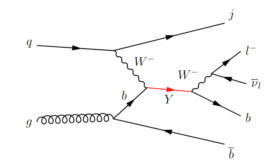
Figure 1: Representative Feynman diagram of single $Y$ (in red) production followed by its subsequent decay $Y\to W^{-}(\to l^{-}\bar{\nu}_{l})b$. Here, $q$ in the initial state represents one of the first two-generation quarks and bottom quark, $j$ in the final state represents one of the first two-generation jets, $b$ in the intermediate (final) state represents a $b$-quark (jet) while $l^{-}$ represents either an electron or muon. Notice that, since we use the five flavor scheme, the $g\to b\bar{b}$ splitting in the diagram is actually accounted for through the PDF evolution.

In Figure 1, we show a representative Feynman diagram of the signal production $pp\to Y\bar{b}j$ and decay chain $Y\to W^{-}(\to l^{-}\bar{\nu}_{l})b$. We expect the $W$ boson and the high-momentum $b$-jet to exhibit a back-to-back alignment in the transverse plane, originating from the decay of the massive $Y$ quark. The topology also encompasses an outgoing light quark, often resulting in a forward jet within the detector. Furthermore, the second $b$-jet arising from the splitting of a gluon into a pair of $b$-quarks can be observed in either the forward or central region. According to these features of signal events, the primary SM backgrounds include $pp\to t\bar{b}j$, $pp\to W^{+}W^{-}b$, $pp\to Zbj$, $pp\to W^{+}bj$, and their charge conjugated processes. Among them, $pp\to t\bar{b}j$ and $pp\to W^{+}W^{-}b$ are irreducible backgrounds, while the others are reducible backgrounds. We have also assessed additional backgrounds, such as $pp\to t\bar{t}$, and found that their contribution can be ignored based on the selection criteria that will be discussed later.

The signal production cross section is determined not only by the mass $m_{Y}$ but also by the coupling strength $\kappa_{Y}$. The cross section is directly proportional to $\kappa_{Y}^{2}$ for a fixed $m_{Y}$ as long as the NWA is met Moretti:2016gkr . In Figure 2, we show the tree-level cross sections for single $Y$ production as a function of the mass $m_{Y}$. We can see that, as $m_{Y}$ increases, the cross section gradually decreases due to a smaller phase space.

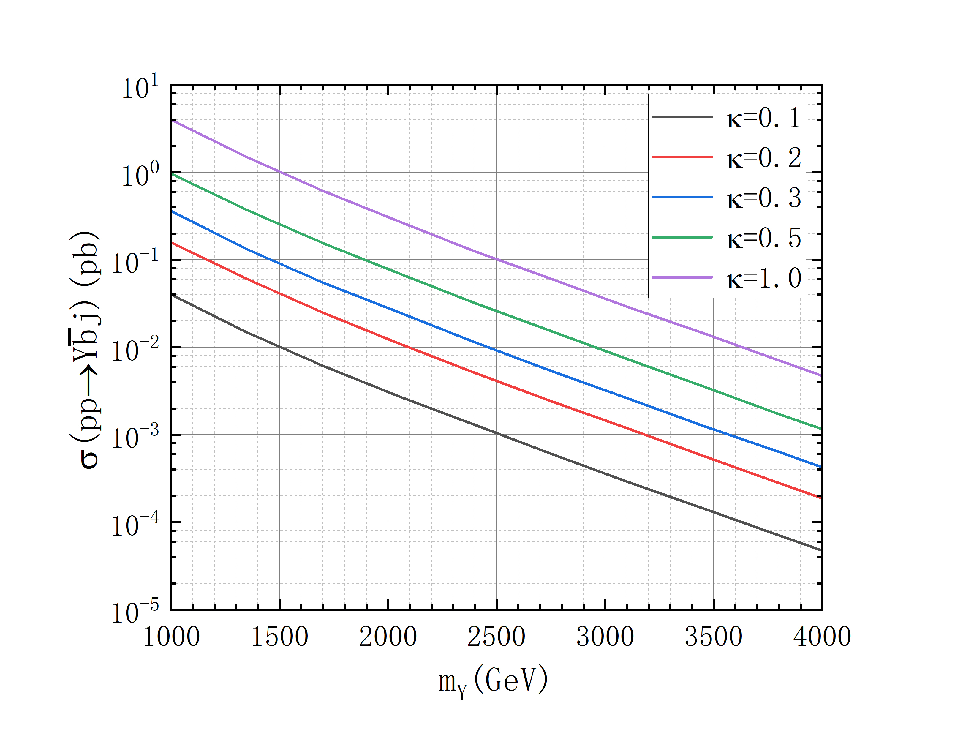
Figure 2: The tree-level cross sections for single $Y$ production as a function of the mass $m_{Y}$ for various values of the coupling $\kappa_{Y}$. The charge conjugated process has also been taken into account.

In Figure 3, we show the tree-level cross sections for the signal benchmarks $m_{Y}=1000\text{ GeV}$ (labeled as $Y_{1000}$) and $m_{Y}=1500\text{ GeV}$ (labeled as $Y_{1500}$) with $\kappa_{Y}=0.1$ and $\kappa_{Y}=0.5$ as well as the tree-level cross sections for the background processes. It is evident that the rates for the latter are significantly larger than those for the former. Consequently, we should design efficient selection criteria (in terms of kinematic cuts) to reduce the number of background events while preserving the signal events. Furthermore, the cross sections for both signal and backgrounds increase with increasing collider energy.

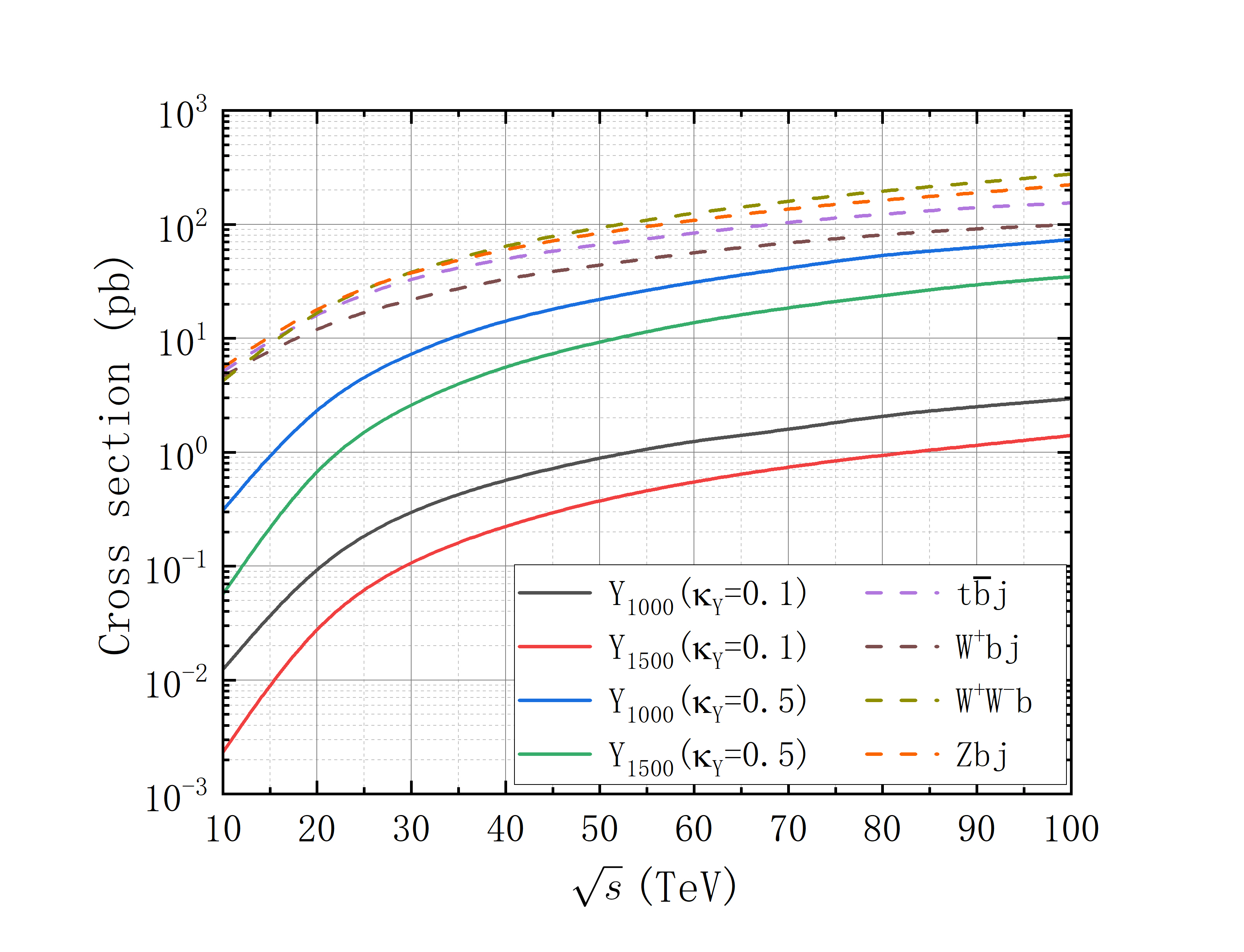
Figure 3: The tree-level cross sections as a function of the center-of-mass energy $\sqrt{s}$ for the signal benchmarks and backgrounds. Solid lines represent the signal processes and dashed lines represent the background processes. The cross sections also include the corresponding charge conjugated processes.

The Next-to-Leading Order (NLO) (or even higher order) QCD corrections for the SM background cross sections at the LHC have been extensively explored in Refs. Czakon:2012zr ; Campbell:2005zv ; Campbell:2006cu ; Kidonakis:2018ncr ; Boos:2012vm . The $K$ factors associated with the background cross sections adopted in our calculations are summarized in Table 2. (Note that, despite they change somewhat with energy, we neglect here changes of $K$ factors values at different colliders, like in Ref. Yang:2022wfa .)

Processes	$Zbj$	$W^{+}bj$	$W^{+}W^{-}b$	$t\bar{b}j$
$K$ factor	1.3 Campbell:2005zv	1.9 Campbell:2006cu	2.1 Campbell:2006cu	1.4 Kidonakis:2018ncr ; Boos:2012vm

Table 2: $K$ factors representing the QCD corrections for the background processes.

There are stringent limits from the oblique parameters $S$, $T$ and $U$ in EWPOs Hollik:1988ii ; Peskin:1990zt ; Grinstein:1991cd ; Peskin:1991sw ; Lavoura:1992np ; Burgess:1993mg ; Maksymyk:1993zm ; Cynolter:2008ea ; 9 ; Chen:2017hak ; Cao:2022mif ; He:2022zjz ; Arsenault:2022xty . These oblique parameters relate to the weak isospin current $J^{\mu}_{1,2,3}$ and the electromagnetic current $J^{\mu}_{Q}=J^{\mu}_{3}+J^{\mu}_{Y}$, involving their vacuum-polarization amplitudes as defined in references Peskin:1990zt ; Peskin:1991sw :

$$S \equiv -\frac{16\pi}{m_{Z}^{2}}\left\{\Sigma_{33}(m_{Z}^{2})-\Sigma_{33}(0)-\Sigma_{3Q}(m_{Z}^{2})\right\}$$ (5)

$$= \frac{16\pi}{m_{Z}^{2}}\left\{\Sigma_{3Y}(m_{Z}^{2})-\Sigma_{3Y}(0)\right\},$$

$$T \equiv \frac{4\pi}{\sin^{2}\theta_{W}\cos^{2}\theta_{W}m_{Z}^{2}}\left\{\Sigma_{33}(0)-\Sigma_{11}(0)\right\},$$ (6)

$$U \equiv \frac{16\pi}{m_{Z}^{2}}\left\{\Sigma_{33}(m_{Z}^{2})-\Sigma_{33}(0)\right\}-\frac{16\pi}{m_{W}^{2}}\left\{\Sigma_{11}(m_{Z}^{2})-\Sigma_{11}(0)\right\},$$ (7)

where $m_{W}$ and $m_{Z}$ denote the mass for $W$ and $Z$ boson, respectively. The $Z$-boson current, represented by $e(J^{\mu}_{3}-s_{W}^{2}J^{\mu}_{Q})/(\sin\theta_{W}\cos\theta_{W})$, involves $e$ linked to the fine-structure constant $\alpha$ through $e^{2}\equiv 4\pi\alpha$. Consequently, the oblique parameters can be reformulated using the vacuum polarizations of the SM gauge bosons as:

$$\alpha T = \frac{\Sigma_{ZZ}^{\rm new}\left(0\right)}{m_{Z}^{2}}-\frac{\Sigma_{WW}^{\rm new}\left(0\right)}{m_{W}^{2}}$$ (8)

$$\frac{\alpha}{\sin^{2}2\theta_{W}}\,S = -\frac{\Sigma_{ZZ}^{\rm new}\left(m_{Z}^{2}\right)-\Sigma_{ZZ}^{\rm new}\left(0\right)}{m_{Z}^{2}}+\left.\frac{\partial\Sigma_{\gamma\gamma}^{\rm new}\left(p^{2}\right)}{\partial p^{2}}\right|_{p^{2}=0}+\frac{\cos 2\theta_{W}}{\cos\theta_{W}\sin\theta_{W}}\left.\frac{\partial\Sigma_{\gamma Z}^{\rm new}\left(p^{2}\right)}{\partial p^{2}}\right|_{p^{2}=0}$$ (9)

$$\simeq \left.-\frac{\partial\Sigma_{ZZ}^{\rm new}\left(p^{2}\right)}{\partial p^{2}}\right|_{p^{2}=0}+\left.\frac{\partial\Sigma_{\gamma\gamma}^{\rm new}\left(p^{2}\right)}{\partial p^{2}}\right|_{p^{2}=0}+\frac{\cos 2\theta_{W}}{\cos\theta_{W}\sin\theta_{W}}\left.\frac{\partial\Sigma_{\gamma Z}^{\rm new}\left(p^{2}\right)}{\partial p^{2}}\right|_{p^{2}=0}$$

$$\frac{\alpha}{4\sin^{2}\theta_{W}}\,U = -\frac{\Sigma_{WW}^{\rm new}\left(m_{W}^{2}\right)-\Sigma_{WW}^{\rm new}\left(0\right)}{m_{W}^{2}}+\cos^{2}\theta_{W}\,\frac{\Sigma_{ZZ}^{\rm new}\left(m_{Z}^{2}\right)-\Sigma_{ZZ}^{\rm new}\left(0\right)}{m_{Z}^{2}}$$ (10)

$$+\sin^{2}\theta_{W}\left.\frac{\partial\Sigma_{\gamma\gamma}^{\rm new}\left(p^{2}\right)}{\partial p^{2}}\right|_{p^{2}=0}+\sin 2\theta_{W}\left.\frac{\partial\Sigma_{\gamma Z}^{\rm new}\left(p^{2}\right)}{\partial p^{2}}\right|_{p^{2}=0}$$

$$\simeq -\frac{\partial\Sigma_{WW}^{\rm new}\left(p^{2}\right)}{\partial p^{2}}|_{p^{2}=0}+\cos^{2}\theta_{W}\frac{\partial\Sigma_{ZZ}^{\rm new}\left(p^{2}\right)}{\partial p^{2}}|_{p^{2}=0}+\sin^{2}\theta_{W}\frac{\partial\Sigma_{\gamma\gamma}^{\rm new}\left(p^{2}\right)}{\partial p^{2}}|_{p^{2}=0}$$

$$+\sin 2\theta_{W}\frac{\partial\Sigma_{\gamma Z}^{\rm new}\left(p^{2}\right)}{\partial p^{2}}|_{p^{2}=0}.$$

The contributions in the doublet $(B,Y)$ model to these oblique parameters can be approximated as follows Cao:2022mif :

$$S\simeq\frac{1}{2\pi}\left\{-\frac{2}{3}\kappa_{Y}^{2}\ln\frac{\mathcal{M}^{2}}{m_{b}^{2}}+\frac{11}{3}\kappa_{Y}^{2}\right\},\,U\simeq-\frac{\kappa_{Y}^{2}}{2\pi},\,T\simeq\frac{3m_{t}^{2}}{8\pi\sin^{2}\theta_{W}m_{W}^{2}}\kappa_{Y}^{4}\frac{2\mathcal{M}^{2}}{3m_{t}^{2}}$$ (11)

Here, $\mathcal{M}^{2}=(m_{Y}^{2}-m_{b}^{2}\kappa_{Y}^{2})/(1-\kappa_{Y}^{2})$ and $m_{W}=m_{Z}\cos\theta_{W}$. For the numerical calculation, the $\chi^{2}$ function for the oblique parameter fit should be less than 8.02 for three degrees of freedom to compute the $2\sigma$ limits, respectively. ${S}=-0.02\pm 0.1$, ${T}=0.03\pm 0.12$, ${U}=0.01\pm 0.11$; there exists a strong correlation of 92% between the $S$ and $T$ parameters, while the U parameter exhibits an anti-correlation of -80% (-93%) with $S$ ($T$)  ParticleDataGroup:2022pth . Specific numerical values of the input parameters are detailed in Eq. 12.

III Signal to background analysis

The signal model file is sourced from FeynRules feynruls and parton-level events are generated using MadGraph5_aMC$@$NLO Alwall:2014hca with the NNPDF23LO1 NNPDF Parton Distribution Function (PDFs). Dynamic factorization and renormalization scales, set as default in MadEvent website_factor , are utilized. Subsequently, fast detector simulations are conducted using Delphes 3.4.2 deFavereau:2013fsa with the built-in detector configurations of the LHC Run-III, HL-LHC, HE-LHC website_hllhc and FCC-hh website_fcchh . Jets are clustered by FastJet Cacciari:2011ma employing the anti-$kt$ algorithm Cacciari:2005hq with a distance parameter of $\Delta R=0.4$. Furthermore, MadAnalysis 5 Conte:2012fm is used to analyze both signal and background events. Finally, the EasyScan_HEP package Shang:2023gfy is utilized to connect these programs and scan the VLQ parameter space.

The numerical values of the input SM parameters are taken as follows ParticleDataGroup:2022pth :

$$m_{b}=4.18{\rm~{}GeV},\quad m_{t}=172.69{\rm~{}GeV},\quad m_{Z}=91.1876{\rm~{}GeV},$$

$$\sin^{2}\theta_{W}=0.22339,\quad\alpha(m_{Z})=\frac{1}{127.951},\quad\alpha_{s}(m_{Z})=0.1179.$$ (12)

Considering the general detection capabilities of detectors, the following basic cuts are chosen:

$$\Delta R(x,y)>0.4 (x,y=l,j,b),$$

$$p^{l}_{T}>25\ {\rm GeV}, \ \ |\eta_{l}|<2.5,$$

$$p^{j}_{T}>20\ {\rm GeV}, \ \ |\eta_{j}|<5.0,$$

$$p^{b}_{T}>25\ {\rm GeV}, \ \ |\eta_{b}|<2.5,$$

where $\Delta R=\sqrt{\Delta\Phi^{2}+\Delta\eta^{2}}$ denotes the separation in the rapidity($\eta$)–azimuth($\phi$) plane.

To handle the relatively small event number of signal ($s$) and background ($b$) events, we will use the median significance $\mathcal{Z}$ to estimate the expected discovery and exclusion reaches Cowan:2010js ; Kumar:2015tna ,

$$\mathcal{Z}_{excl}=\sqrt{2\left[s-b\ln\left(\frac{b+s+x}{2b}\right)-\frac{1}{\delta^{2}}\ln\left(\frac{b-s+x}{2b}\right)\right]-(b+s-x)\left(1+\frac{1}{\delta^{2}b}\right)},$$ (13)

$$\mathcal{Z}_{disc}=\sqrt{2\left[(s+b)\ln\left(\frac{(s+b)(1+\delta^{2}b}{b+(s+b)\delta^{2}b}\right)-\frac{1}{\delta^{2}}\ln\left(1+\frac{\delta^{2}s}{1+\delta^{2}b}\right)\right]},$$ (14)

$$x=\sqrt{(s+b)^{2}-\frac{4\delta^{2}sb^{2}}{1+\delta^{2}b}},$$ (15)

where $\delta$ is the uncertainty that inevitably appears in the measurement of the background. In the completely ideal case, that is $\delta$=0, Eq. (13) and (14) can be simplified as follows, respectively:

$$\mathcal{Z}_{excl}=\sqrt{2\left[s-b\ln\left(1+\frac{s}{b}\right)\right]},$$ (16)

and

$$\mathcal{Z}_{disc}=\sqrt{2\left[(s+b)\ln\left(1+\frac{s}{b}\right)-s\right]}.$$ (17)

III.1 LHC Run-III and HL-LHC

Firstly, we establish a trigger that emulates the LHC Run-III and HL-LHC detector response based on the count of final state particles detected in each event. Given the limited efficiency of the detector in identifying jets, we adopt a lenient approach towards the number of jets. Consequently, the final trigger criteria are defined as follows: $N_{l}=1$, $N_{j}\geq 2$, $N_{j}\leq 4$ and $N_{b}\geq 2$.

Considering that the mass of $Y$ is notably greater than that of its decay products, the latter exhibit distinct spatial characteristics in pseudorapidity $\eta$ and spatial separation $\Delta R$ compared to backgrounds. These differences inform our selection criteria.

Cuts	$Y_{1500}$ (fb)	$Y_{1800}$ (fb)	$t\bar{b}j$   (fb)	$W^{+}bj$  (fb)	$W^{+}W^{-}b$  (fb)	$Zbj$  (fb)
Basic Cuts	1.99	0.97	13855.00	15016.00	18967.00	13897.00
Trigger	0.29	0.13	2227.40	775.10	1251.50	312.80
Cut 1	0.25	0.12	40.09	11.95	39.12	2.63
Cut 2	0.23	0.11	7.46	4.07	8.07	0.63
Cut 3	0.16	0.08	4.51	3.02	4.93	0.39
Cut 4	0.08	0.05	0.08	1.35	1.18	0.15
Cut 5	0.08	0.04	0.08	1.00	0.89	0.13
Cut 6	0.04	0.03	0.01	0.02	0.05	0.00
Cut 7	0.03	0.02	0.01	0.00	0.03	0.00

Table 3: Cut flows of the signal with $\kappa_{Y}=0.1$ and backgrounds at the 14 TeV HL-LHC, where the conjugate processes $pp\to\bar{t}bj$, $W^{-}\bar{b}j$, $W^{+}W^{-}\bar{b}$, $Z\bar{b}j$ have been included.

Furthermore, since the mass range of $Y$ is much heavier than the particles originating from background processes, we anticipate that the transverse momentum (referred to as $\vec{p}_{T}$ and its magnitude denoted as $p_{T}$) of decay products of the $Y$ state will be substantially larger than those of the same particles from background processes. Besides, we will also consider variables such as $\not{E}_{T}$, $\not{H}_{T}$ and $M_{T}$ to distinguish the signal from the background. Here, $\not{E}_{T}$ represents the magnitude of the sum of the transverse momenta of all visible final state particles, $\not{H}_{T}$ is analogous to $\not{E}_{T}$ but only considers all visible hadronic momenta while the transverse mass $M_{T}$ is defined as follows:

$$M_{T}^{2} \equiv[E_{T}(1)+E_{T}(2)]^{2}-[\vec{p}_{T}(1)+\vec{p}_{T}(2)]^{2}$$

$$=m_{1}^{2}+m_{2}^{2}+2[E_{T}(1)E_{T}(2)-\vec{p}_{T}(1)\cdot\vec{p}_{T}(2)],$$

where $E_{T}(i)=\sqrt{p^{2}_{T}(i)+m^{2}_{i}}$ and $m^{2}_{i}=p_{i}^{2}$ with $p_{i}$ representing a 4-vector.

In Figure 4, we present the normalized distributions of $p_{T}^{j_{1}}$, $M_{b_{1}l_{1}}$, $M_{j_{1}j_{2}}$, $M_{T}^{b_{2}l_{1}}$, $M_{T}^{b_{1}l_{1}}$, $\Delta R_{j_{1},b_{1}}$, $\not{H}_{T}$ and $\not{E}_{T}$ for both $m_{Y}=1500\text{ GeV}$ and $m_{Y}=1800\text{ GeV}$ with $\kappa_{Y}=0.1$ as well as for the background processes. Based on these distributions, we have devised the following selection criteria to distinguish the signal from the various backgrounds:

• Trigger: $N_{l}=1$, $N_{j}\geq 2$, $N_{j}\leq 4$, and $N_{b}\geq 2$;

• Cut-1: $p_{T}^{j_{1}}>300\text{ GeV}$;

• Cut-2: $M_{b_{1}l_{1}}>500\text{ GeV}$;

• Cut-3: $M_{j_{1}j_{2}}>500\text{ GeV}$;

• Cut-4: $M_{T}^{b_{1}l_{1}}>200\text{ GeV}$ and $M_{T}^{b_{2}l_{1}}>200\text{ GeV}$;

• Cut-5: $\Delta R_{j_{1},b_{1}}<1.0$;

• Cut-6: $\not{H}_{T}>600\text{ GeV}$;

• Cut-7: $\not{E}_{T}>200\text{ GeV}$.

By applying these cuts, we can see that the signal efficiencies for $m_{Y}=1500\text{ GeV}$ and $m_{Y}=1800\text{ GeV}$ are 1.35% and 2.41%, respectively. The higher efficiency for the latter can be attributed to the larger transverse boost of the final state originating from an heavier $Y$. Meanwhile, the background processes are significantly suppressed. For reference, we provide the cut flows in Table 3.

We present the exclusion capability ($\mathcal{Z}_{\text{excl}}=2$) and discovery potential ($\mathcal{Z}_{\text{disc}}=5$) for $Y$ with two different integrated luminosities, 1000 fb^-1 and 3000 fb^-1, at the HL-LHC, as shown in the top line of Figure 7. This analysis considers both the ideal scenario without systematic uncertainties and the case with a 10% systematic uncertainty. In the presence of 10% systematic uncertainty, the $Y$ can be excluded in the correlated parameter space of $\kappa_{Y}\in[0.044,0.5]$ and $m_{Y}\in[1000\text{ GeV},3099\text{ GeV}]$ with an integrated luminosity of $L=300\text{ fb}^{-1}$, which corresponds to the maximum achievable integrated luminosity during LHC Run-III. If the integrated luminosity is raised to 3000 fb^-1, aligning with the maximum achievable at the HL-LHC, the excluded parameter zones extend to $\kappa_{Y}\in[0.027,0.5]$ and $m_{Y}\in[1000\text{ GeV},3653\text{ GeV}]$. Furthermore, the discovery regions are $\kappa_{Y}\in[0.072,0.5]$ ([0.047, 0.5]) and $m_{Y}\in[1000\text{ GeV},2621\text{ GeV}]$ ($[1000\text{ GeV},3047\text{ GeV}]$) with $L=300\text{ fb}^{-1}$ (3000 fb^-1).

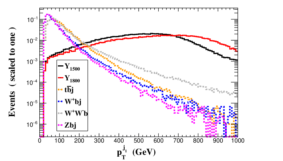
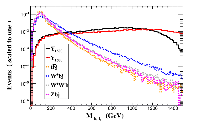
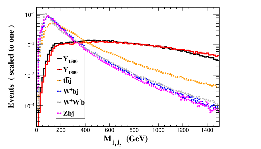
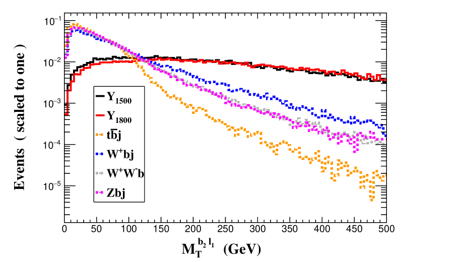
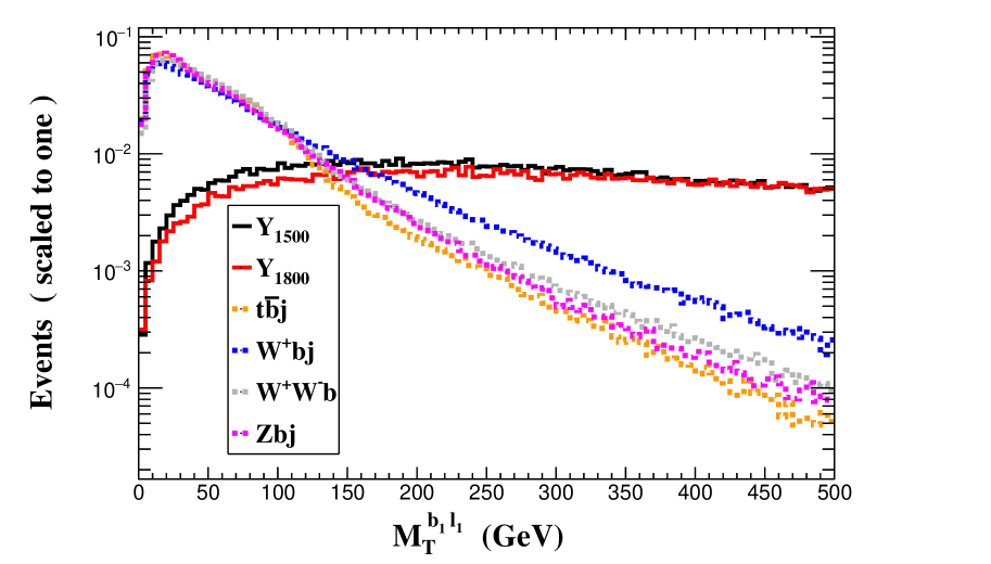
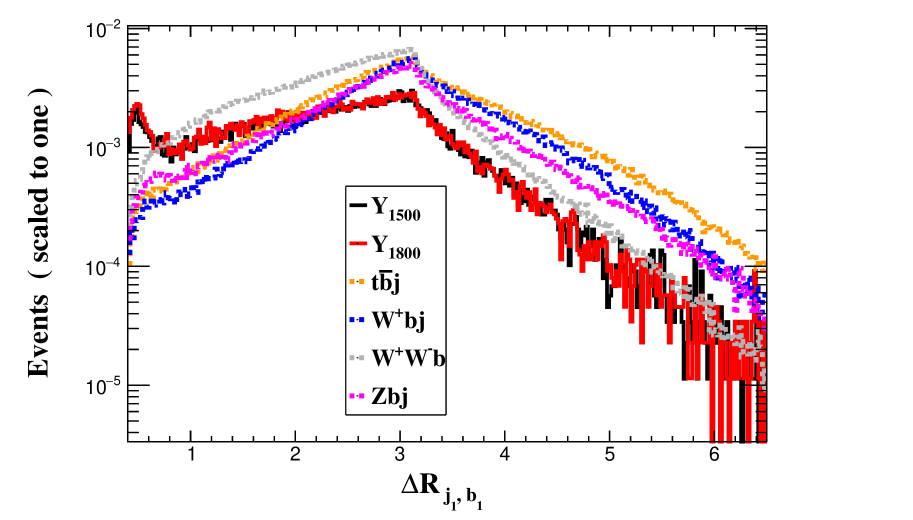
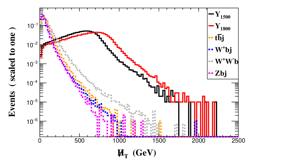
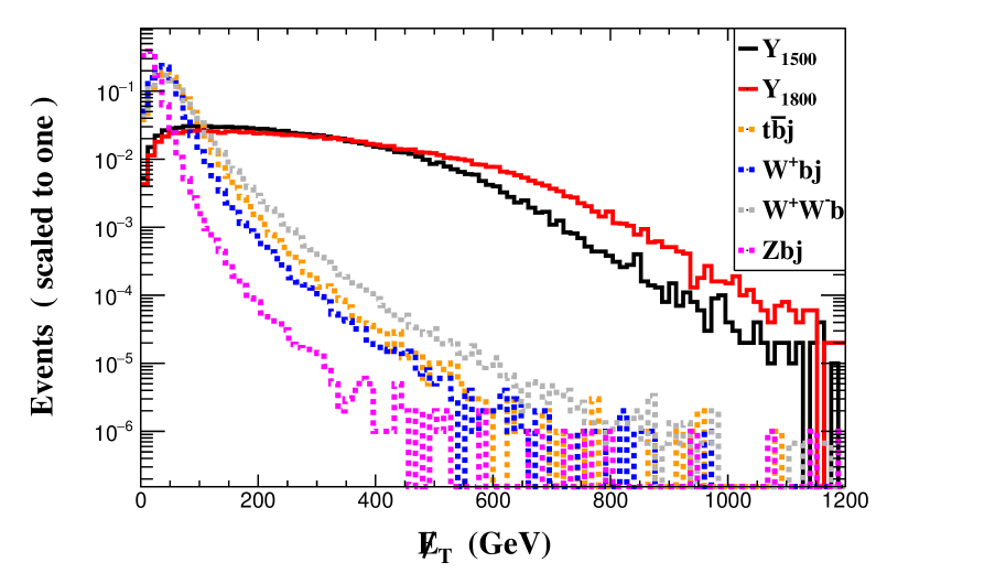
Figure 4: Normalized distributions for the signals of $m_{Y}=$ 1500 GeV and 1800 GeV and SM backgrounds at the HL-LHC. The conjugated processes have been included.

III.2 27 TeV HE-LHC

Cuts	$Y_{1500}$ (fb)	$Y_{1800}$ (fb)	$t\bar{b}j$   (fb)	$W^{+}bj$  (fb)	$W^{+}W^{-}b$  (fb)	$Zbj$  (fb)
Basic Cuts	16.86	10.01	41398.00	38670.00	69303.00	69658.00
Trigger	1.78	0.10	6224.50	2149.10	4445.40	1700.70
Cut 1	1.50	0.91	86.07	29.51	133.60	10.73
Cut 2	1.36	0.85	18.30	11.14	29.52	2.37
Cut 3	0.95	0.62	12.83	9.05	19.27	1.53
Cut 4	0.35	0.27	0.17	2.94	3.10	0.35
Cut 5	0.33	0.25	0.17	2.01	2.36	0.28
Cut 6	0.12	0.16	0.00	0.04	0.37	0.00
Cut 7	0.09	0.12	0.00	0.04	0.14	0.00

Table 4: Cut flows of the signal with $\kappa_{Y}=0.1$ and backgrounds at the 27 TeV HE-LHC.

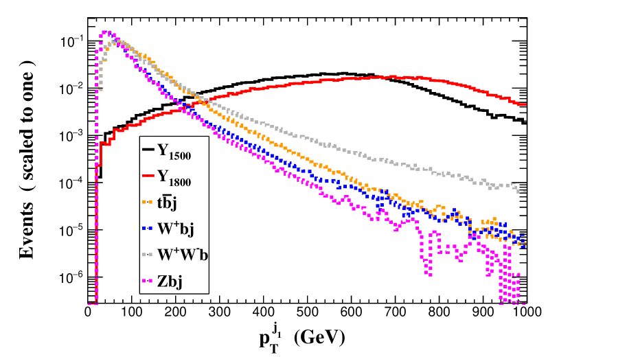
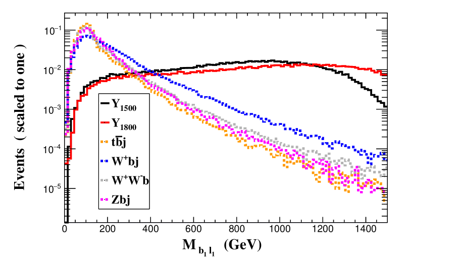
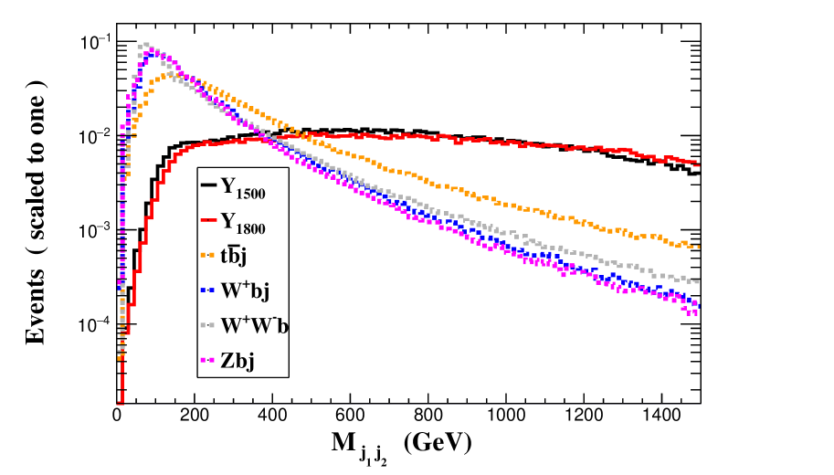
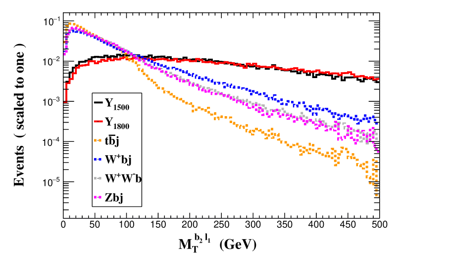
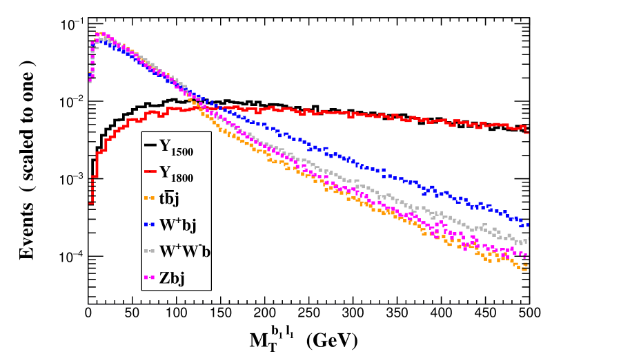
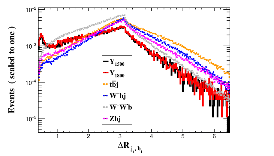
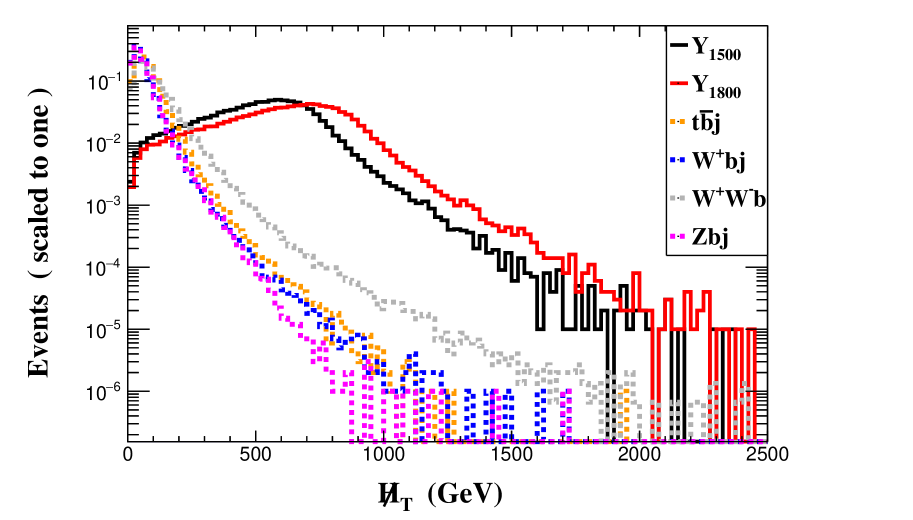
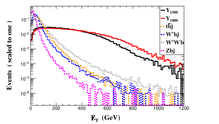
Figure 5: Normalized distributions for the signals with $m_{Y}=$ 1500 GeV and 1800 GeV and backgrounds at the HE-LHC.

This section delves into the prospective signal of $Y$ at the future 27 TeV HE-LHC. In Figure 5, we exhibit the normalized distributions for both signal and background processes, forming the basis for our distinctive selection criteria:

• Trigger: $N_{l}=1$, $N_{j}\geq 2$, $N_{j}\leq 4$, and $N_{b}\geq 2$;

• Cut-1: $p_{T}^{j_{1}}>350\text{ GeV}$;

• Cut-2: $M_{b_{1}l_{1}}>550\text{ GeV}$;

• Cut-3: $M_{j_{1}j_{2}}>550\text{ GeV}$;

• Cut-4: $M_{T}^{b_{2}l_{1}}>250\text{ GeV}$ and $M_{T}^{b_{1}l_{1}}>250\text{ GeV}$;

• Cut-5: $\Delta R_{j_{1},b_{1}}<0.5$;

• Cut-6: $\not{H}_{T}>650\text{ GeV}$;

• Cut-7: $\not{E}_{T}>200\text{ GeV}$.

The kinematic variables remain consistent with those of the 14 TeV case, but the cut threshold values for transverse momentum-based variables, such as $\not{H}_{T}>650\text{ GeV}$, are higher than those in the 14 TeV case. This adjustment accounts for the increased center-of-mass energy. Detailed cut flows are outlined in Table 4 and the exclusion capability and discovery potential are shown in the second row of Figure 7. The $Y$ quark can be excluded within the correlated parameter space of $\kappa_{Y}\in[0.033,0.5]$ and $m_{Y}\in[1000\text{ GeV},4783\text{ GeV}]$ with 10% systematic uncertainty for $L=1000\text{ fb}^{-1}$. If the integrated luminosity is raised to the highest designed value 10 ab^-1, the excluded parameter regions can be extended to $\kappa_{Y}\in[0.029,0.5]$ and $m_{Y}\in[1000\text{ GeV},4987\text{ GeV}]$. For $L=3000\text{ fb}^{-1}$, the discovery regions are $\kappa_{Y}\in[0.053,0.5]$ and $m_{Y}\in[1000\text{ GeV},3885\text{ GeV}]$. If the integrated luminosity is raised to the highest designed value 10 ab^-1, the discovery parameter regions can be extended to $\kappa_{Y}\in[0.051,0.5]$ and $m_{Y}\in[1000\text{ GeV},3943\text{ GeV}]$.

III.3 100 TeV FCC-hh

Cuts	$Y_{1500}$ (fb)	$Y_{1800}$ (fb)	$t\bar{b}j$   (fb)	$W^{+}bj$  (fb)	$W^{+}W^{-}b$  (fb)	$Zbj$  (fb)
Basic Cuts	261.26	183.18	237538.00	206093.00	573258.00	291603.00
Trigger	13.44	8.42	33633.00	17209.00	40939.00	6363.90
Cut 1	6.37	4.20	209.30	112.70	605.90	18.95
Cut 2	5.63	3.89	54.16	48.43	163.30	7.58
Cut 3	3.30	2.51	3.33	23.91	53.74	3.21
Cut 4	3.14	2.43	3.33	17.72	45.12	3.21
Cut 5	1.40	1.70	0.48	1.65	6.15	0.00
Cut 6	0.81	1.16	0.24	0.21	2.87	0.00

Table 5: Cut flows of the signal with $\kappa_{Y}=0.1$ and backgrounds at the 100 TeV FCC-hh.

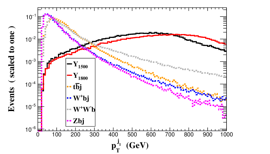
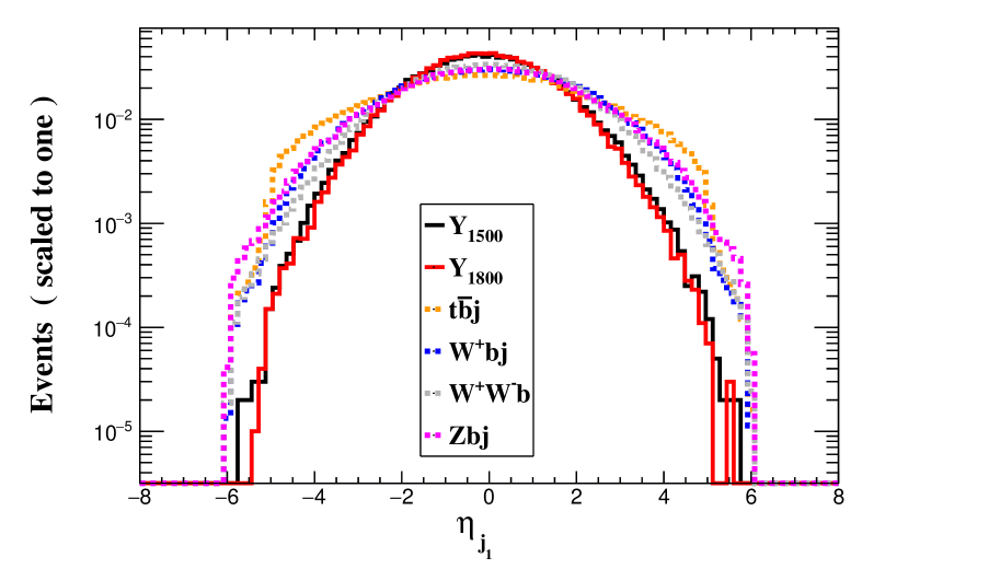
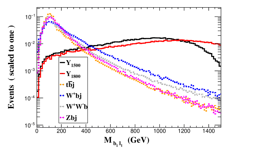
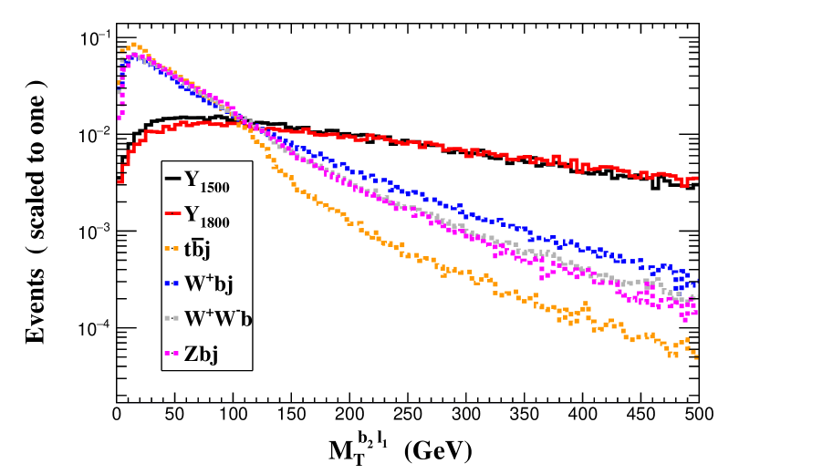
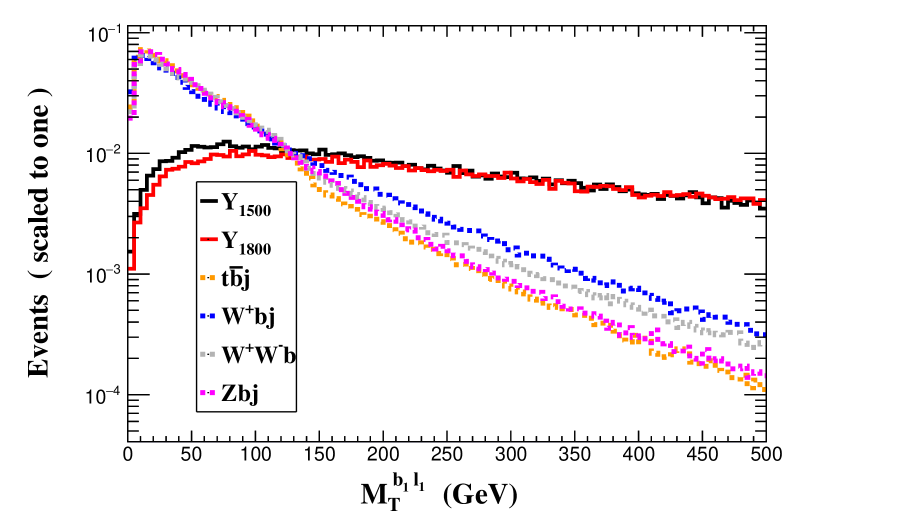
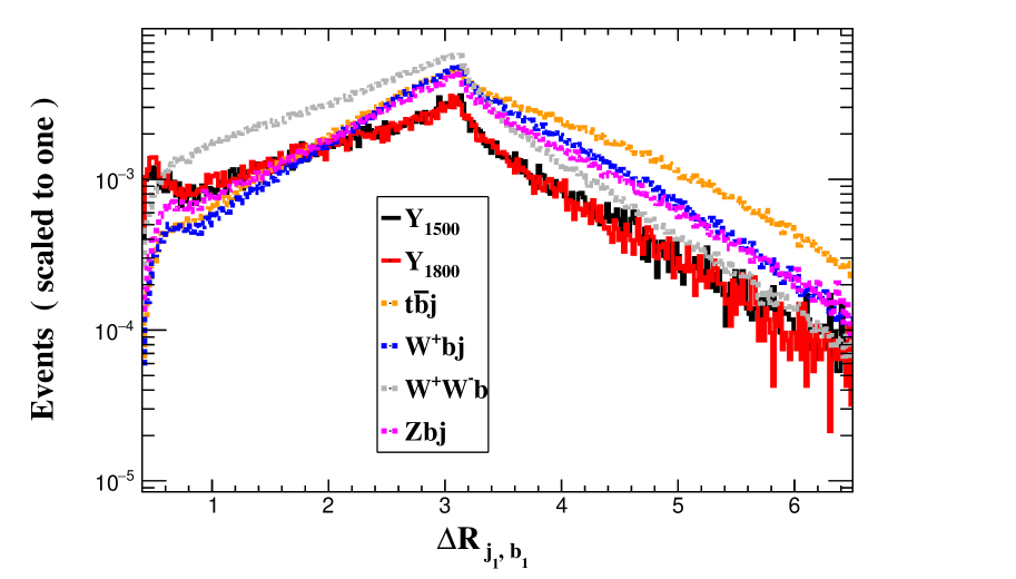
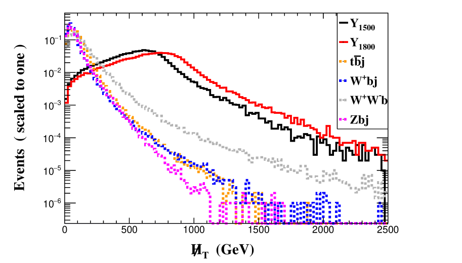
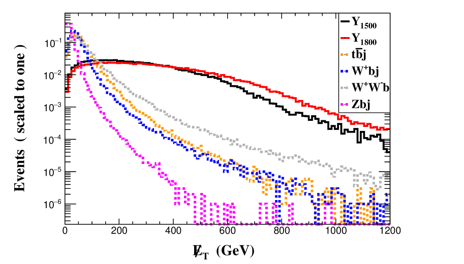
Figure 6: Normalized distributions for the signals with $m_{Y}=$ 1500 GeV and 1800 GeV, and backgrounds at the FCC-hh.

Here, we explore the anticipated signal of ${Y}$ in the context of the future 100 TeV FCC-hh. The figures in Figure 6 portray normalized distributions for both signal and background processes, laying the groundwork for our distinctive selection criteria:

• Trigger: $N_{l}=1$, $N_{j}\geq 2$, $N_{j}\leq 4$, and $N_{b}\geq 2$;

• Cut-1: $p_{T}^{j_{1}}>350\text{ GeV}$, $|\eta_{j_{1}}|<1$;

• Cut-2: $M_{b_{1},l_{1}}>550\text{ GeV}$;

• Cut-3: $M_{T}^{b_{2}l_{1}}>150\text{ GeV}$ and $M_{T}^{b_{1}l_{1}}>250\text{ GeV}$;

• Cut-4: $\Delta R_{j_{1},b_{1}}<0.5\text{ GeV}$;

• Cut-5: $\not{H}_{T}>650\text{ GeV}$;

• Cut-6: $\not{E}_{T}>300\text{ GeV}$.

Compared to previous cases, an additional variable, $\eta_{j_{1}}$, is introduced here. Upon analyzing the distributions of $\eta_{j_{1}}$, it is apparent that the signal tends to be more central than the backgrounds. Thus, we require $|\eta_{j_{1}}|<1$. The signal efficiencies for $m_{Y}=1500\text{ GeV}$ and $m_{Y}=1800\text{ GeV}$ are 0.20% and 0.45%, respectively. Notably, there is a significant suppression in the background processes. Comprehensive cut flows are provided in Table 5. The exclusion capability and discovery potential are illustrated in the final row of Figure 7. It is evident that systematic uncertainty has a considerable impact on the results. Even with a 10% systematic uncertainty, the parameter space region will significantly shrink. Accounting for the 10% systematic uncertainty, the $Y$ quark can be excluded within the correlated parameter space of $\kappa_{Y}\in[0.051,0.5]$ and $m_{Y}\in[1000\text{ GeV},6610\text{ GeV}]$ at the highest design value of luminosity, $L=30\text{ ab}^{-1}$. Additionally, the $Y$ state can be discovered within $\kappa_{Y}\in[0.088,0.5]$ and $m_{Y}\in[1000\text{ GeV},4624\text{ GeV}]$ at $L=30\text{ ab}^{-1}$.

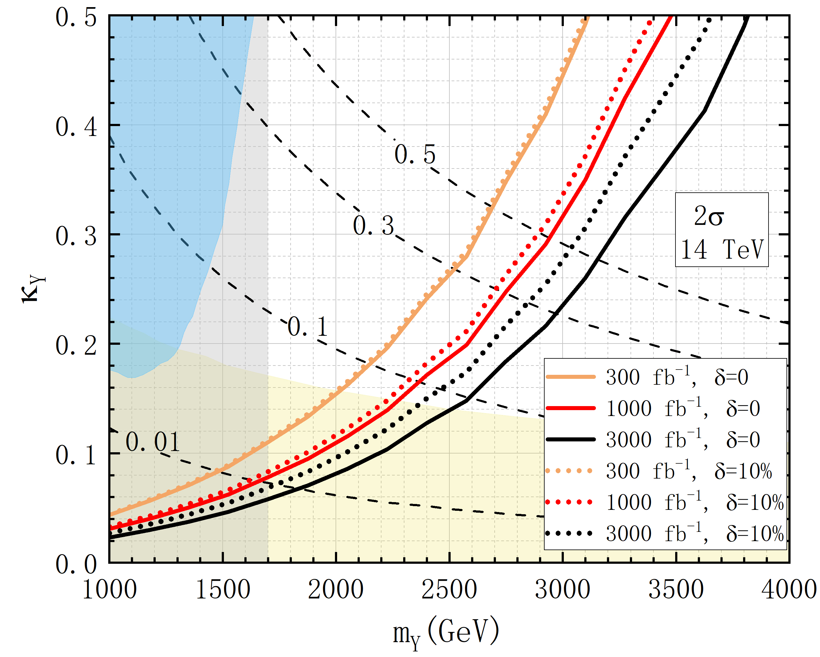
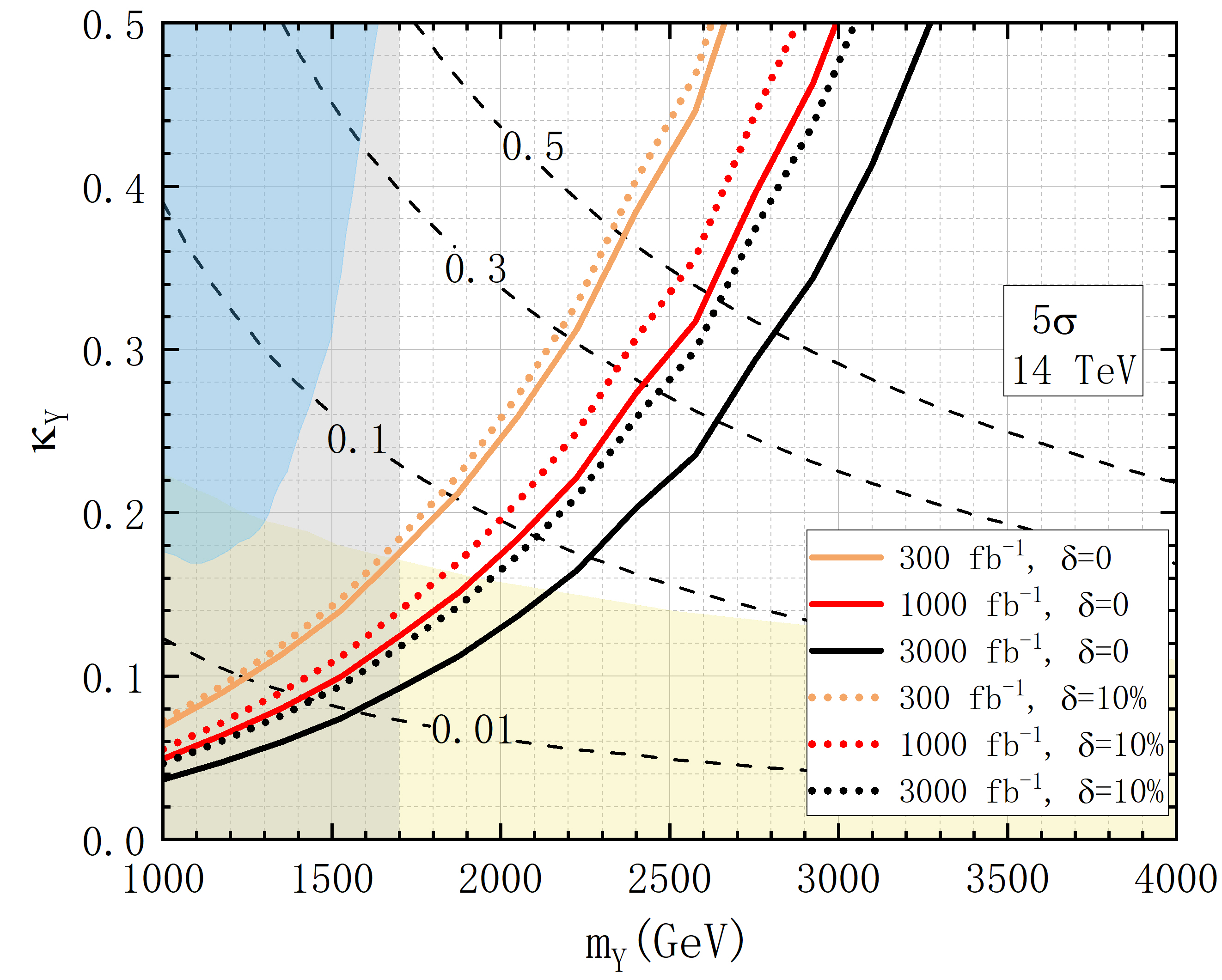
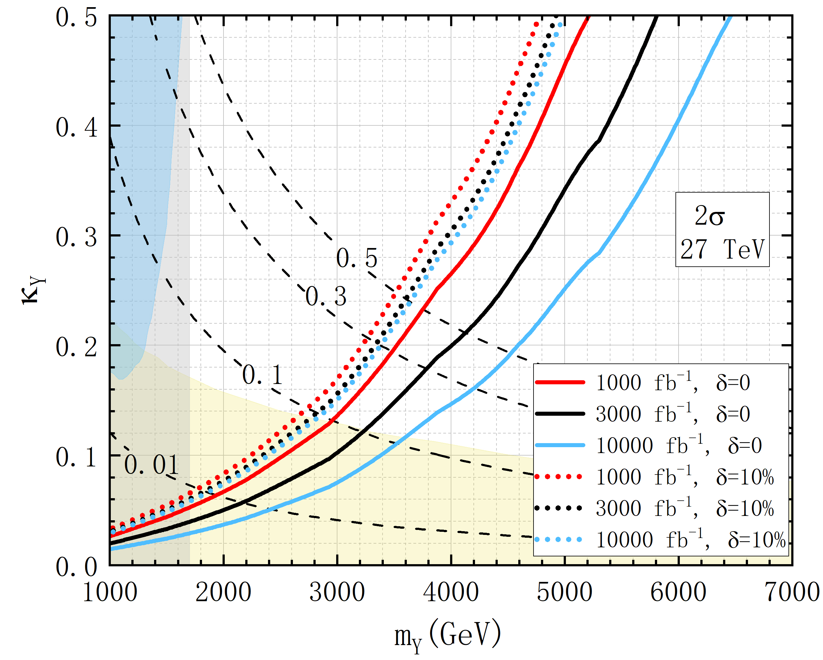
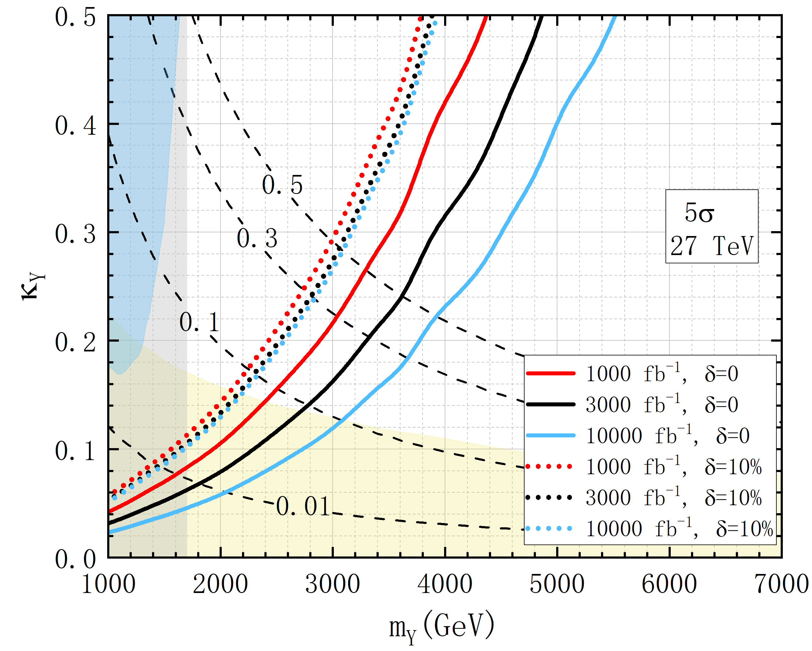
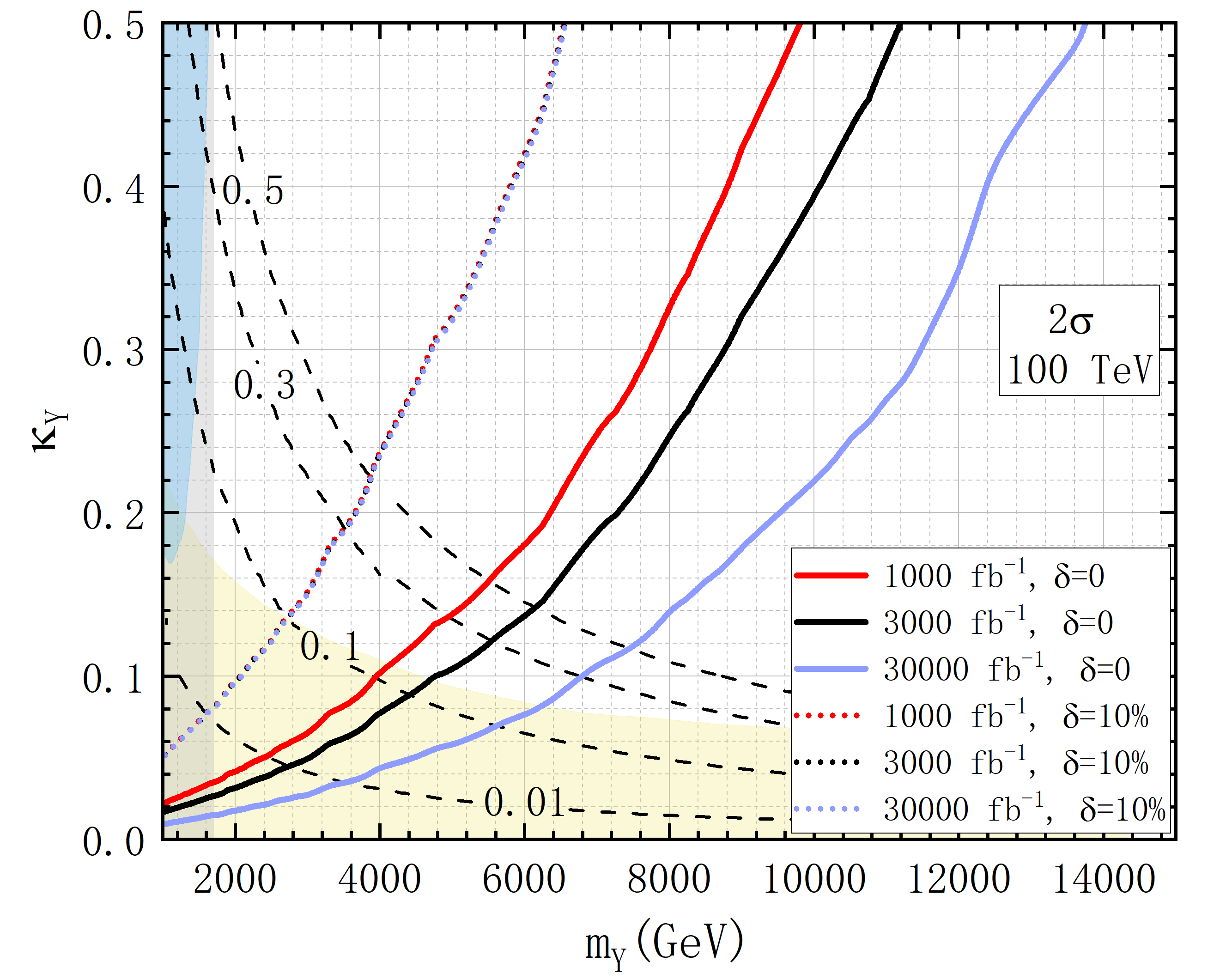
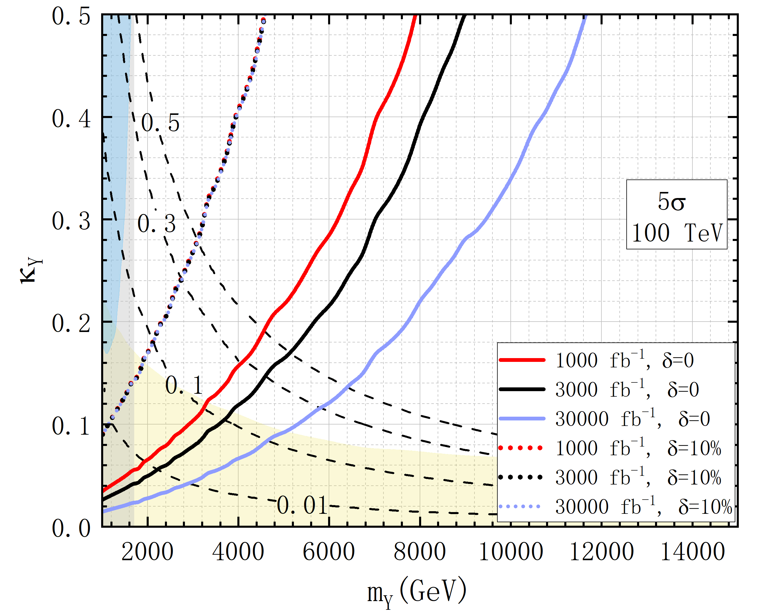
Figure 7: The exclusion capability ($\mathcal{Z}_{\text{excl}}=2$) and discovery potential ($\mathcal{Z}_{\text{disc}}=5$) for the $Y$ state at the LHC Run-III and HL-LHC, $\sqrt{s}=27\text{ TeV}$ HE-LHC and $\sqrt{s}=100\text{ TeV}$ FCC-hh. Solid lines represent the ideal scenario without systematic uncertainty, the dotted lines represent the scenario with a 10% systematic uncertainty. Dashed lines denote the contours of $\Gamma_{Y}/m_{Y}$. The blue (grey) shaded area indicates the exclusion region of the current LHC at $\sqrt{s}=$ 13 TeV with $L=$36.1 fb^-1 (140 fb^-1), as reported in Ref. ATLAS:2018dyh (Ref. ATLAS:2023shy ). Meanwhile, the yellow shaded area denotes the allowed region for the oblique parameters $S,T$ and $U$, considering the current measurements in Ref. ParticleDataGroup:2022pth .

IV Summary

Colliders	$L/\text{fb}^{-1}$	Uncertainty	Exclusion		Discovery
			$\kappa_{Y}$	$m_{Y}$(GeV)	$\kappa_{Y}$	$m_{Y}$(GeV)
LHC Run-III	300	0	[0.043,0.5]	[1000,3111]	[0.069,0.5]	[1000,2665]
	300	10%	[0.044,0.5]	[1000,3099]	[0.072,0.5]	[1000,2621]
14 TeV HL-LHC	1000	0	[0.031,0.5]	[1000,3486]	[0.049,0.5]	[1000,2988]
	3000	0	[0.023,0.5]	[1000,3820]	[0.037,0.5]	[1000,3267]
	1000	10%	[0.033,0.5]	[1000,3398]	[0.055,0.5]	[1000,2880]
	3000	10%	[0.027,0.5]	[1000,3653]	[0.047,0.5]	[1000,3047]
	1000	0	[0.026,0.5]	[1000,5213]	[0.042,0.5]	[1000,4359]
27 TeV HE-LHC	3000	0	[0.020,0.5]	[1000,5811]	[0.031,0.5]	[1000,4863]
	10000	0	[0.015,0.5]	[1000,6476]	[0.024,0.5]	[1000,5513]
	1000	10%	[0.033,0.5]	[1000,4783]	[0.057,0.5]	[1000,3783]
	3000	10%	[0.030,0.5]	[1000,4936]	[0.053,0.5]	[1000,3885]
	10000	10%	[0.029,0.5]	[1000,4987]	[0.051,0.5]	[1000,3943]
	1000	0	[0.022,0.5]	[1000,9953]	[0.035,0.5]	[1000,7933]
	3000	0	[0.016,0.5]	[1000,11259]	[0.026,0.5]	[1000,9000]
100 TeV FCC-hh	10000	0	[0.014,0.5]	[1000,12254]	[0.021,0.5]	[1000,10425]
	30000	0	[0.010,0.5]	[1000,13771]	[0.015,0.5]	[1000,11649]
	1000	10%	[0.051,0.5]	[1000,6610]	[0.088,0.5]	[1000,4624]
	3000	10%	[0.051,0.5]	[1000,6610]	[0.088,0.5]	[1000,4624]
	10000	10%	[0.051,0.5]	[1000,6610]	[0.088,0.5]	[1000,4624]
	30000	10%	[0.051,0.5]	[1000,6610]	[0.088,0.5]	[1000,4624]

Table 6: Summary for 2$\sigma$ exclusion limits and 5$\sigma$ signal discoveries at the LHC Run-III and HL-LHC, $\sqrt{s}=27\text{ TeV}$ HE-LHC and $\sqrt{s}=100\text{ TeV}$ FCC-hh.

In a simplified model, we have investigated the single production of a doublet VLQ denoted by $Y$ in the $Wb$ decay channel at the the $\sqrt{s}=14$ TeV HL-LHC, $\sqrt{s}=27$ TeV HE-LHC and $\sqrt{s}=100$ TeV FCC-hh, following its production via $pp\to Ybj$, with the $W$ decaying leptonically (into electrons and muons plus their respective neutrinos). We have performed a detector level simulation for the signal and relevant SM backgrounds. Considering a systematic uncertainty of 10% with an integrated luminosity of 3000 fb^-1, the exclusion and discovery capabilities, as displayed in Table VI, can be described as follows: (1) The HL-LHC can exclude (discover) the correlated regions of $\kappa_{Y}\in[0.027,0.5]$ $([0.047,0.5])$ and $m_{Y}\in[1000\text{ GeV},3653\text{ GeV}]$ $([1000\text{ GeV},3047\text{ GeV}])$; (2) The HE-LHC can exclude (discover) the correlated regions of $\kappa_{Y}\in[0.030,0.5]$ $([0.053,0.5])$ and $m_{Y}\in[1000\text{ GeV},4936\text{ GeV}]$ $([1000\text{ GeV},3885\text{ GeV}])$; (3) The FCC-hh can exclude (discover) the correlated regions of $\kappa_{Y}\in[0.051,0.5]$ $([0.088,0.5])$ and $m_{Y}\in[1000\text{ GeV},6610\text{ GeV}]$ $([1000\text{ GeV},4624\text{ GeV}])$.

Furthermore, we highlight that the stringent constraint on the VLQ $Y$, derived from the $Y$ pair production search with BR($Y\to W^{-}b$) $=1$, imposes $m_{Y}>1700\text{ GeV}$. In this context, we reassess the potential of LHC Run-III to explore the VLQ $Y$, revealing that the associated parameter regions of $\kappa_{Y}\in[0.044,0.5]$ $([0.072,0.5])$ and $m_{Y}\in[1000\text{ GeV},3099\text{ GeV}]$ $([1000\text{ GeV},2621\text{ GeV}])$ can be excluded (discovered) based on LHC Run-III luminosity. We foresee that our investigation will spur complementary explorations for a potential $Y$ quark at forthcoming $pp$ colliders.

Appendix A Appendix: Relationship between Eq. (1) and Eq. (3)

In the appendix, we provide the relationship between the $(B,Y)$ doublet representation and the simplified model used in the simulation. However, we do not present the relationship between the $(X,B,Y)$ triplet representation and the simplified model here because it can be easily derived from the remainder of this Appendix.)

The Lagrangian for the $Y$ coupling with the SM gauge fields and the $Y$ mass term is

$$\mathcal{L}=\bar{Q}_{5}(i\not{D}-M_{F})Q_{5}$$ (A.1)

where one has

$$Q_{5}=\begin{pmatrix}B_{0}\\ Y_{0}\end{pmatrix},\bar{Q}_{5}=(\bar{B}_{0},\bar{Y}_{0}),\not{D}=\gamma^{\mu}D_{\mu},D_{\mu}=\partial_{\mu}+i{g}^{\prime}Y_{F}B_{\mu}+\frac{i}{2}g\tau^{I}W_{\mu}^{I}$$ (A.2)

and the weak isospin $g$ and weak hypercharge $g^{\prime}$ are the SU(2)_L and U(1)_Y couplings, respectively. We use a subscript $0$ to represent the interaction eigenstates. The unphysical fields $B_{\mu}$ and $W^{I}_{\mu}$ ($I=1,2,3$) can be transformed into the physical fields of the photon $A_{\mu}$, the neutral $Z$ boson $Z_{\mu}$ and charged $W$ bosons $W^{\pm}_{\mu}$ via the following equations:

$$B_{\mu} =\cos\theta_{W}A_{\mu}-\sin\theta_{W}Z_{\mu},W^{3}_{\mu}=\sin\theta_{W}A_{\mu}+\cos\theta_{W}Z_{\mu},$$

$$W^{1}_{\mu} =\frac{1}{\sqrt{2}}(W^{+}_{\mu}+W^{-}_{\mu}),W^{2}_{\mu}=\frac{i}{\sqrt{2}}(W^{+}_{\mu}-W^{-}_{\mu})$$ (A.3)

where $\theta_{W}$ is the Weinberg angle, which can be expressed via $\sin\theta_{W}=\frac{e}{g}$ and $\cos\theta_{W}=\frac{e}{g^{\prime}}$. Here, $M_{F}$ is a free mass parameter. Considering the charge of $Y$, the Lagrangian for the $Y$ coupling with the SM gauge fields is

$$\mathcal{L}_{Q_{5}Q_{5}V} =\bar{Q}_{5}\left(\frac{5}{6}{g}^{\prime}B_{\mu}-\frac{g}{2}\begin{bmatrix}W_{\mu}^{3}&W_{\mu}^{1}-iW_{\mu}^{2}\\ W_{\mu}^{1}+iW_{\mu}^{2}&-W_{\mu}^{3}\end{bmatrix}\right)\gamma^{\mu}Q_{5}$$

$$=\bar{Q}_{5}\begin{bmatrix}\frac{1}{3}eA_{\mu}-\frac{g}{2\cos\theta}\left(1+\frac{2}{3}\sin^{2}\theta\right)Z_{\mu}&-\frac{g}{\sqrt{2}}W_{\mu}^{+}\\ -\frac{g}{\sqrt{2}}W_{\mu}^{-}&\frac{4}{3}eA_{\mu}+\frac{g}{2\cos\theta}\left(1-\frac{8}{3}\sin^{2}\theta\right)Z_{\mu}\end{bmatrix}\gamma^{\mu}Q_{5}$$

$$=\frac{1}{3}e\bar{B}_{0}A_{\mu}\gamma^{\mu}B_{0}-\frac{g}{2\cos\theta}\left(1+\frac{2}{3}\sin^{2}\theta\right)\bar{B}_{0}Z_{\mu}\gamma^{\mu}B_{0}$$

$$\,\,\,\,\,\,+\frac{4}{3}e\bar{Y}_{0}A_{\mu}\gamma^{\mu}Y_{0}+\frac{g}{2\cos\theta}\left(1-\frac{8}{3}\sin^{2}\theta\right)\bar{Y}_{0}Z_{\mu}\gamma^{\mu}Y_{0}$$

$$\,\,\,\,\,\,-\frac{g}{\sqrt{2}}\bar{Y}_{0}W^{-}_{\mu}\gamma^{\mu}B_{0}-\frac{g}{\sqrt{2}}\bar{B}_{0}W^{+}_{\mu}\gamma^{\mu}Y_{0}.$$ (A.4)

In our study, $(B,Y)$ states exclusively couple with the third-generation quarks of the SM. Therefore, the Lagrangian for the mass term of the bottom quark mass eigenstate $b$ and its partner mass eigenstate $B$ can be written as

$$\mathcal{L}_{\text{mass}}=-\begin{pmatrix}\bar{b}_{0}^{L}&\bar{B}_{0}^{L}\end{pmatrix}\begin{pmatrix}y_{33}^{d}\frac{v}{\sqrt{2}}&y_{34}^{d}\frac{v}{\sqrt{2}}\\ y_{43}^{d}\frac{v}{\sqrt{2}}&M^{0}\end{pmatrix}\begin{pmatrix}b_{0}^{R}\\ B_{0}^{R}\end{pmatrix}+\text{H.c.}$$ (A.5)

where $v=246\text{ GeV}$ is the Vacuum Expectation Value (VEV) of the Higgs field, $M^{0}$ is a bare mass term, $y_{33}^{d}$ and $y_{43}^{d}$ are Yukawa coupling coefficients while $y_{34}^{d}=0$ for doublets. The mass matrix can be diagonalized by the two mixing matrices $V^{L}$ and $V^{R}$, as follows:

$$\begin{pmatrix}b_{0}^{L,R}\\ B_{0}^{L,R}\end{pmatrix}=V^{L,R}\begin{pmatrix}b^{L,R}\\ B^{L,R}\end{pmatrix}$$ (A.6)

where $L$ and $R$ stands for the left-hand and right-hand chiralities, respectively. There exists the following relationship too: $B_{0}=B_{0}^{L}+B_{0}^{R}$ and $Y_{0}=Y_{0}^{L}+Y_{0}^{R}$. The $2\times 2$ unitary matrices $V^{L}$ and $V^{R}$ can be parameterized by the mixing angles $\theta^{L}$ and $\theta^{R}$, respectively, as

$$V^{L,R}=\begin{pmatrix}\cos\theta^{L,R}&\sin\theta^{L,R}\\ -\sin\theta^{L,R}&\cos\theta^{L,R}\end{pmatrix}$$ (A.7)

We can then determine the expressions $B_{0}^{L,R}=-\sin\theta^{L,R}b^{L,R}+\cos\theta^{L,R}B^{L,R}$. For $Y$, it is as simple as $Y_{0}^{L,R}=Y^{L,R}$, where $Y$ represents the mass eigenstate. This is because there are no $\pm 4/3$ particles in the SM. Therefore, we can derive the interactions between the $Y$, $W$ and $b$ states as follows:

$$\mathcal{L}_{YW^{\pm}b} =-\frac{g}{\sqrt{2}}\left(\bar{Y}^{L}+\bar{Y}^{R}\right)W^{-}_{\mu}\gamma^{\mu}\left(-\sin\theta^{L}b^{L}-\sin\theta^{R}b^{R}\right)+\text{H.c.}$$

$$=\frac{g}{\sqrt{2}}\sin\theta^{L}\bar{Y}^{L}W^{-}_{\mu}\gamma^{\mu}b^{L}+\frac{g}{\sqrt{2}}\sin\theta^{R}\bar{Y}^{R}W^{-}_{\mu}\gamma^{\mu}b^{R}+\text{H.c.}$$ (A.8)

Using unitary matrices, we can finally obtain

$$V^{L}\begin{pmatrix}y_{33}^{d}\frac{v}{\sqrt{2}}&y_{34}^{d}\frac{v}{\sqrt{2}}\\ y_{43}^{d}\frac{v}{\sqrt{2}}&M^{0}\end{pmatrix}(V^{R})^{\dagger}=\begin{pmatrix}m_{b}&0\\ 0&m_{B}\end{pmatrix}$$ (A.9)

After performing calculations involving trigonometric function identities, we can obtain:

$$\tan\theta^{L}=\frac{m_{b}}{m_{B}}\tan\theta^{R}$$ (A.10)

Since $m_{B}\gg m_{b}$, we can conclude that $\sin\theta^{L}\gg\sin\theta^{R}$ in the ($B,Y$) doublet. Therefore, our study primarily concentrates on the right-handed coupling part of the interactions involving the $Y$, $W$ and $b$ states.

References

- (1) ATLAS Collaboration, G. Aad et al., “Observation of a new particle in the search for the Standard Model Higgs boson with the ATLAS detector at the LHC,” Phys. Lett. B 716 (2012) 1–29, arXiv:1207.7214 [hep-ex].
- (2) CMS Collaboration, S. Chatrchyan et al., “Observation of a New Boson at a Mass of 125 GeV with the CMS Experiment at the LHC,” Phys. Lett. B 716 (2012) 30–61, arXiv:1207.7235 [hep-ex].
- (3) N. Arkani-Hamed, A. G. Cohen, E. Katz, and A. E. Nelson, “The Littlest Higgs,” JHEP 07 (2002) 034, arXiv:hep-ph/0206021.
- (4) T. Han, H. E. Logan, B. McElrath, and L.-T. Wang, “Phenomenology of the little Higgs model,” Phys. Rev. D 67 (2003) 095004, arXiv:hep-ph/0301040.
- (5) S. Chang and H.-J. He, “Unitarity of little Higgs models signals new physics of UV completion,” Phys. Lett. B 586 (2004) 95–105, arXiv:hep-ph/0311177.
- (6) Q.-H. Cao and C.-R. Chen, “Signatures of extra gauge bosons in the littlest Higgs model with T-parity at future colliders,” Phys. Rev. D 76 (2007) 075007, arXiv:0707.0877 [hep-ph].
- (7) K. Agashe, G. Perez, and A. Soni, “Collider Signals of Top Quark Flavor Violation from a Warped Extra Dimension,” Phys. Rev. D 75 (2007) 015002, arXiv:hep-ph/0606293.
- (8) K. Agashe, R. Contino, and A. Pomarol, “The Minimal composite Higgs model,” Nucl. Phys. B 719 (2005) 165–187, arXiv:hep-ph/0412089.
- (9) B. Bellazzini, C. Csáki, and J. Serra, “Composite Higgses,” Eur. Phys. J. C 74 no. 5, (2014) 2766, arXiv:1401.2457 [hep-ph].
- (10) M. Low, A. Tesi, and L.-T. Wang, “Twin Higgs mechanism and a composite Higgs boson,” Phys. Rev. D 91 (2015) 095012, arXiv:1501.07890 [hep-ph].
- (11) L. Bian, D. Liu, and J. Shu, “Low scale composite Higgs model and 1.8 2 TeV diboson excess,” Int. J. Mod. Phys. A 33 no. 11, (2018) 1841007, arXiv:1507.06018 [hep-ph].
- (12) H.-J. He, C. T. Hill, and T. M. P. Tait, “Top Quark Seesaw, Vacuum Structure and Electroweak Precision Constraints,” Phys. Rev. D 65 (2002) 055006, arXiv:hep-ph/0108041.
- (13) H.-J. He, T. M. P. Tait, and C. P. Yuan, “New top flavor models with seesaw mechanism,” Phys. Rev. D 62 (2000) 011702, arXiv:hep-ph/9911266.
- (14) H.-J. He, T. M. P. Tait, and C. P. Yuan, “New top flavor models with seesaw mechanism,” Phys. Rev. D 62 (2000) 011702, arXiv:hep-ph/9911266.
- (15) X.-F. Wang, C. Du, and H.-J. He, “LHC Higgs Signatures from Topflavor Seesaw Mechanism,” Phys. Lett. B 723 (2013) 314–323, arXiv:1304.2257 [hep-ph].
- (16) H.-J. He, C. T. Hill, and T. M. P. Tait, “Top Quark Seesaw, Vacuum Structure and Electroweak Precision Constraints,” Phys. Rev. D 65 (2002) 055006, arXiv:hep-ph/0108041.
- (17) J. A. Aguilar-Saavedra, R. Benbrik, S. Heinemeyer, and M. Pérez-Victoria, “Handbook of vectorlike quarks: Mixing and single production,” Phys. Rev. D 88 no. 9, (2013) 094010, arXiv:1306.0572 [hep-ph].
- (18) A. Banerjee, V. Ellajosyula, and L. Panizzi, “Heavy vector-like quarks decaying to exotic scalars: a case study with triplets,” arXiv:2311.17877 [hep-ph].
- (19) R. Benbrik, M. Berrouj, M. Boukidi, A. Habjia, E. Ghourmin, and L. Rahili, “Search for single production of vector-like top partner T → H+b and H→tb¯ at the LHC Run-III,” Phys. Lett. B 843 (2023) 138024.
- (20) Q.-G. Zeng, Y.-S. Pan, and J. Zhang, “Search for the signal of vector-like bottom quark at LHeC in the final state with 3 -jets,” Nucl. Phys. B 995 (2023) 116347.
- (21) A. C. Canbay and O. Cakir, “Investigating the single production of vectorlike quarks decaying into a top quark and W boson through hadronic channels at the HL-LHC,” Phys. Rev. D 108 no. 9, (2023) 095006, arXiv:2307.12883 [hep-ph].
- (22) A. Belyaev, R. S. Chivukula, B. Fuks, E. H. Simmons, and X. Wang, “Vectorlike top quark production via an electroweak dipole moment at a muon collider,” Phys. Rev. D 108 no. 3, (2023) 035016, arXiv:2306.11097 [hep-ph].
- (23) L. Shang and K. Sun, “Single vector-like quark X production in the tW channel at high energy pp colliders,” Nucl. Phys. B 990 (2023) 116185.
- (24) B. Yang, S. Wang, X. Sima, and L. Shang, “Singlet vector-like quark production in association with b at the CLIC,” Commun. Theor. Phys. 75 no. 3, (2023) 035202.
- (25) A. Bhardwaj, T. Mandal, S. Mitra, and C. Neeraj, “Roadmap to explore vectorlike quarks decaying to a new scalar or pseudoscalar,” Phys. Rev. D 106 no. 9, (2022) 095014, arXiv:2203.13753 [hep-ph].
- (26) A. Bhardwaj, K. Bhide, T. Mandal, S. Mitra, and C. Neeraj, “Discovery prospects of a vectorlike top partner decaying to a singlet boson,” Phys. Rev. D 106 no. 7, (2022) 075024, arXiv:2204.09005 [hep-ph].
- (27) J. Bardhan, T. Mandal, S. Mitra, and C. Neeraj, “Machine learning-enhanced search for a vectorlike singlet B quark decaying to a singlet scalar or pseudoscalar,” Phys. Rev. D 107 no. 11, (2023) 115001, arXiv:2212.02442 [hep-ph].
- (28) L. Shang, C. Chen, S. Wang, and B. Yang, “Single production of vector-like B quark decaying into bZ at future ep colliders,” Nucl. Phys. B 984 (2022) 115977.
- (29) F. F. Freitas, J. a. Gonçalves, A. P. Morais, and R. Pasechnik, “Phenomenology at the large hadron collider with deep learning: the case of vector-like quarks decaying to light jets,” Eur. Phys. J. C 82 no. 9, (2022) 826, arXiv:2204.12542 [hep-ph].
- (30) R. Benbrik, M. Boukidi, and S. Moretti, “Probing Light Charged Higgs Bosons in the 2-Higgs Doublet Model Type-II with Vector-Like Quarks,” arXiv:2211.07259 [hep-ph].
- (31) G. Corcella, A. Costantini, M. Ghezzi, L. Panizzi, G. M. Pruna, and J. Šalko, “Vector-like quarks decaying into singly and doubly charged bosons at LHC,” JHEP 10 (2021) 108, arXiv:2107.07426 [hep-ph].
- (32) G. Corcella, A. Costantini, M. Ghezzi, L. Panizzi, G. M. Pruna, and J. Šalko, “Vector-like quarks decaying into singly and doubly charged bosons at LHC,” JHEP 10 (2021) 108, arXiv:2107.07426 [hep-ph].
- (33) A. Belyaev, R. S. Chivukula, B. Fuks, E. H. Simmons, and X. Wang, “Vectorlike top quark production via a chromomagnetic moment at the LHC,” Phys. Rev. D 104 no. 9, (2021) 095024, arXiv:2107.12402 [hep-ph].
- (34) A. Deandrea, T. Flacke, B. Fuks, L. Panizzi, and H.-S. Shao, “Single production of vector-like quarks: the effects of large width, interference and NLO corrections,” JHEP 08 (2021) 107, arXiv:2105.08745 [hep-ph]. [Erratum: JHEP 11, 028 (2022)].
- (35) S. Dasgupta, R. Pramanick, and T. S. Ray, “Broad toplike vector quarks at LHC and HL-LHC,” Phys. Rev. D 105 no. 3, (2022) 035032, arXiv:2112.03742 [hep-ph].
- (36) S. J. D. King, S. F. King, S. Moretti, and S. J. Rowley, “Discovering the origin of Yukawa couplings at the LHC with a singlet Higgs and vector-like quarks,” JHEP 21 (2020) 144, arXiv:2102.06091 [hep-ph].
- (37) Y.-B. Liu and S. Moretti, “Search for single production of a top quark partner via the and channels at the LHC,” Phys. Rev. D 100 no. 1, (2019) 015025, arXiv:1902.03022 [hep-ph].
- (38) R. Benbrik et al., “Signatures of vector-like top partners decaying into new neutral scalar or pseudoscalar bosons,” JHEP 05 (2020) 028, arXiv:1907.05929 [hep-ph].
- (39) K.-P. Xie, G. Cacciapaglia, and T. Flacke, “Exotic decays of top partners with charge 5/3: bounds and opportunities,” JHEP 10 (2019) 134, arXiv:1907.05894 [hep-ph].
- (40) N. Bizot, G. Cacciapaglia, and T. Flacke, “Common exotic decays of top partners,” JHEP 06 (2018) 065, arXiv:1803.00021 [hep-ph].
- (41) G. Cacciapaglia, A. Carvalho, A. Deandrea, T. Flacke, B. Fuks, D. Majumder, L. Panizzi, and H.-S. Shao, “Next-to-leading-order predictions for single vector-like quark production at the LHC,” Phys. Lett. B 793 (2019) 206–211, arXiv:1811.05055 [hep-ph].
- (42) G. Cacciapaglia, A. Deandrea, N. Gaur, D. Harada, Y. Okada, and L. Panizzi, “The LHC potential of Vector-like quark doublets,” JHEP 11 (2018) 055, arXiv:1806.01024 [hep-ph].
- (43) A. Carvalho, S. Moretti, D. O’Brien, L. Panizzi, and H. Prager, “Single production of vectorlike quarks with large width at the Large Hadron Collider,” Phys. Rev. D 98 no. 1, (2018) 015029, arXiv:1805.06402 [hep-ph].
- (44) CMS Collaboration, A. M. Sirunyan et al., “Search for single production of vector-like quarks decaying to a b quark and a Higgs boson,” JHEP 06 (2018) 031, arXiv:1802.01486 [hep-ex].
- (45) D. Barducci and L. Panizzi, “Vector-like quarks coupling discrimination at the LHC and future hadron colliders,” JHEP 12 (2017) 057, arXiv:1710.02325 [hep-ph].
- (46) CMS Collaboration, A. M. Sirunyan et al., “Search for single production of a vector-like T quark decaying to a Z boson and a top quark in proton-proton collisions at = 13 TeV,” Phys. Lett. B 781 (2018) 574–600, arXiv:1708.01062 [hep-ex].
- (47) C.-H. Chen and T. Nomura, “Single production of and vectorlike quarks at the LHC,” Phys. Rev. D 94 no. 3, (2016) 035001, arXiv:1603.05837 [hep-ph].
- (48) A. Arhrib, R. Benbrik, S. J. D. King, B. Manaut, S. Moretti, and C. S. Un, “Phenomenology of 2HDM with vectorlike quarks,” Phys. Rev. D 97 (2018) 095015, arXiv:1607.08517 [hep-ph].
- (49) G. Cacciapaglia, A. Deandrea, N. Gaur, D. Harada, Y. Okada, and L. Panizzi, “Interplay of vector-like top partner multiplets in a realistic mixing set-up,” JHEP 09 (2015) 012, arXiv:1502.00370 [hep-ph].
- (50) A. Angelescu, A. Djouadi, and G. Moreau, “Vector-like top/bottom quark partners and Higgs physics at the LHC,” Eur. Phys. J. C 76 no. 2, (2016) 99, arXiv:1510.07527 [hep-ph].
- (51) L. Panizzi, “Vector-like quarks: and partners,” Nuovo Cim. C 037 no. 02, (2014) 69–79.
- (52) L. Panizzi, “Model-independent Analysis of Scenarios with Vector-like Quarks,” Acta Phys. Polon. Supp. 7 no. 3, (2014) 631.
- (53) G. Cacciapaglia, A. Deandrea, L. Panizzi, S. Perries, and V. Sordini, “Heavy Vector-like quark with charge 5/3 at the LHC,” JHEP 03 (2013) 004, arXiv:1211.4034 [hep-ph].
- (54) Y. Okada and L. Panizzi, “LHC signatures of vector-like quarks,” Adv. High Energy Phys. 2013 (2013) 364936, arXiv:1207.5607 [hep-ph].
- (55) G. Cacciapaglia, A. Deandrea, L. Panizzi, N. Gaur, D. Harada, and Y. Okada, “Heavy Vector-like Top Partners at the LHC and flavour constraints,” JHEP 03 (2012) 070, arXiv:1108.6329 [hep-ph].
- (56) F. del Aguila, L. Ametller, G. L. Kane, and J. Vidal, “Vector Like Fermion and Standard Higgs Production at Hadron Colliders,” Nucl. Phys. B 334 (1990) 1–23.
- (57) F. Gianotti et al., “Physics potential and experimental challenges of the LHC luminosity upgrade,” Eur. Phys. J. C 39 (2005) 293–333, arXiv:hep-ph/0204087.
- (58) “High-Luminosity Large Hadron Collider (HL-LHC): Technical Design Report V. 0.1,”.
- (59) FCC Collaboration, A. Abada et al., “HE-LHC: The High-Energy Large Hadron Collider: Future Circular Collider Conceptual Design Report Volume 4,” Eur. Phys. J. ST 228 no. 5, (2019) 1109–1382.
- (60) FCC Collaboration, A. Abada et al., “FCC-hh: The Hadron Collider: Future Circular Collider Conceptual Design Report Volume 3,” Eur. Phys. J. ST 228 no. 4, (2019) 755–1107.
- (61) ATLAS Collaboration, M. Aaboud et al., “Search for single production of vector-like quarks decaying into in collisions at TeV with the ATLAS detector,” JHEP 05 (2019) 164, arXiv:1812.07343 [hep-ex].
- (62) CMS Collaboration, A. M. Sirunyan et al., “Search for single production of vector-like quarks decaying into a b quark and a W boson in proton-proton collisions at 13 TeV,” Phys. Lett. B 772 (2017) 634–656, arXiv:1701.08328 [hep-ex].
- (63) ATLAS Collaboration, “Search for pair-production of vector-like quarks in lepton+jets final states containing at least one -jet using the Run 2 data from the ATLAS experiment,”.
- (64) J. Cao, L. Meng, L. Shang, S. Wang, and B. Yang, “Interpreting the W-mass anomaly in vectorlike quark models,” Phys. Rev. D 106 no. 5, (2022) 055042, arXiv:2204.09477 [hep-ph].
- (65) CDF Collaboration, T. Aaltonen et al., “High-precision measurement of the boson mass with the CDF II detector,” Science 376 no. 6589, (2022) 170–176.
- (66) M. Buchkremer, G. Cacciapaglia, A. Deandrea, and L. Panizzi, “Model Independent Framework for Searches of Top Partners,” Nucl. Phys. B 876 (2013) 376–417, arXiv:1305.4172 [hep-ph].
- (67) V. Cetinkaya, A. Ozansoy, V. Ari, O. M. Ozsimsek, and O. Cakir, “Single production of vectorlike Y quarks at the HL-LHC,” Nucl. Phys. B 973 (2021) 115580, arXiv:2012.15308 [hep-ph].
- (68) D. Berdine, N. Kauer, and D. Rainwater, “Breakdown of the Narrow Width Approximation for New Physics,” Phys. Rev. Lett. 99 (2007) 111601, arXiv:hep-ph/0703058.
- (69) S. Moretti, D. O’Brien, L. Panizzi, and H. Prager, “Production of extra quarks at the Large Hadron Collider beyond the Narrow Width Approximation,” Phys. Rev. D 96 no. 7, (2017) 075035, arXiv:1603.09237 [hep-ph].
- (70) M. Czakon and A. Mitov, “NNLO corrections to top-pair production at hadron colliders: the all-fermionic scattering channels,” JHEP 12 (2012) 054, arXiv:1207.0236 [hep-ph].
- (71) J. M. Campbell, R. K. Ellis, F. Maltoni, and S. Willenbrock, “Production of a boson and two jets with one heavy-quark tag,” Phys. Rev. D 73 (2006) 054007, arXiv:hep-ph/0510362. [Erratum: Phys.Rev.D 77, 019903 (2008)].
- (72) J. M. Campbell, R. K. Ellis, F. Maltoni, and S. Willenbrock, “Production of a boson and two jets with one quark tag,” Phys. Rev. D 75 (2007) 054015, arXiv:hep-ph/0611348.
- (73) N. Kidonakis, “Single-top production in the Standard Model and beyond,” in 13th Conference on the Intersections of Particle and Nuclear Physics. 8, 2018. arXiv:1808.02934 [hep-ph].
- (74) E. Boos and L. Dudko, “The Single Top Quark Physics,” Int. J. Mod. Phys. A 27 (2012) 1230026, arXiv:1211.7146 [hep-ph].
- (75) B. Yang, X. Sima, S. Wang, and L. Shang, “Single vectorlike top quark production in the tZ channel at high energy pp colliders,” Phys. Rev. D 105 no. 9, (2022) 096010.
- (76) W. F. L. Hollik, “Radiative Corrections in the Standard Model and their Role for Precision Tests of the Electroweak Theory,” Fortsch. Phys. 38 (1990) 165–260.
- (77) M. E. Peskin and T. Takeuchi, “A New constraint on a strongly interacting Higgs sector,” Phys. Rev. Lett. 65 (1990) 964–967.
- (78) B. Grinstein and M. B. Wise, “Operator analysis for precision electroweak physics,” Phys. Lett. B 265 (1991) 326–334.
- (79) M. E. Peskin and T. Takeuchi, “Estimation of oblique electroweak corrections,” Phys. Rev. D 46 (1992) 381–409.
- (80) L. Lavoura and J. P. Silva, “The Oblique corrections from vector - like singlet and doublet quarks,” Phys. Rev. D 47 (1993) 2046–2057.
- (81) C. P. Burgess, S. Godfrey, H. Konig, D. London, and I. Maksymyk, “A Global fit to extended oblique parameters,” Phys. Lett. B 326 (1994) 276–281, arXiv:hep-ph/9307337.
- (82) I. Maksymyk, C. P. Burgess, and D. London, “Beyond S, T and U,” Phys. Rev. D 50 (1994) 529–535, arXiv:hep-ph/9306267.
- (83) G. Cynolter and E. Lendvai, “Electroweak Precision Constraints on Vector-like Fermions,” Eur. Phys. J. C 58 (2008) 463–469, arXiv:0804.4080 [hep-ph].
- (84) C.-Y. Chen, S. Dawson, and E. Furlan, “Vectorlike fermions and Higgs effective field theory revisited,” Phys. Rev. D 96 no. 1, (2017) 015006, arXiv:1703.06134 [hep-ph].
- (85) S.-P. He, “Leptoquark and vector-like quark extended model for simultaneousexplanation of W boson mass and muon g–2 anomalies*,” Chin. Phys. C 47 no. 4, (2023) 043102, arXiv:2205.02088 [hep-ph].
- (86) A. Arsenault, K. Y. Cingiloglu, and M. Frank, “Vacuum stability in the Standard Model with vectorlike fermions,” Phys. Rev. D 107 no. 3, (2023) 036018, arXiv:2207.10332 [hep-ph].
- (87) Particle Data Group Collaboration, R. L. Workman et al., “Review of Particle Physics,” PTEP 2022 (2022) 083C01.
- (88) A. Alloul, N. D. Christensen, C. Degrande, C. Duhr, and B. Fuks, “FeynRules 2.0 - A complete toolbox for tree-level phenomenology,” Comput. Phys. Commun. 185 (2014) 2250–2300, arXiv:1310.1921 [hep-ph].
- (89) J. Alwall, R. Frederix, S. Frixione, V. Hirschi, F. Maltoni, O. Mattelaer, H. S. Shao, T. Stelzer, P. Torrielli, and M. Zaro, “The automated computation of tree-level and next-to-leading order differential cross sections, and their matching to parton shower simulations,” JHEP 07 (2014) 079, arXiv:1405.0301 [hep-ph].
- (90) NNPDF Collaboration, R. D. Ball et al., “Parton distributions from high-precision collider data,” Eur. Phys. J. C 77 no. 10, (2017) 663, arXiv:1706.00428 [hep-ph].
- (91) J. Alwall, R. Frederix, S. Frixione, V. Hirschi, F. Maltoni, O. Mattelaer, H. S. Shao, T. Stelzer, P. Torrielli, and M. Zaro, “What are the default dynamic factorization and renormalization scales in madevent?” 2011. https://cp3.irmp.ucl.ac.be/projects/madgraph/wiki/FAQ-General-13. Accessed on 2023-12-25.
- (92) DELPHES 3 Collaboration, J. de Favereau, C. Delaere, P. Demin, A. Giammanco, V. Lemaître, A. Mertens, and M. Selvaggi, “DELPHES 3, A modular framework for fast simulation of a generic collider experiment,” JHEP 02 (2014) 057, arXiv:1307.6346 [hep-ex].
- (93) CERN Collaboration, M. Selvaggi, “Delphes cards for LHC Run-III, HL-LHC and HE-LHC.” December 6th, 2017. https://github.com/delphes/delphes/blob/master/cards/delphes_card_HLLHC.tcl. Accessed on 2023-12-25.
- (94) CERN Collaboration, M. Selvaggi, “Delphes card for FCC-hh.” October 14th, 2020. https://github.com/delphes/delphes/blob/master/cards/FCC/FCChh.tcl. Accessed on 2023-12-25.
- (95) M. Cacciari, G. P. Salam, and G. Soyez, “FastJet User Manual,” Eur. Phys. J. C 72 (2012) 1896, arXiv:1111.6097 [hep-ph].
- (96) M. Cacciari and G. P. Salam, “Dispelling the myth for the jet-finder,” Phys. Lett. B 641 (2006) 57–61, arXiv:hep-ph/0512210.
- (97) E. Conte, B. Fuks, and G. Serret, “MadAnalysis 5, A User-Friendly Framework for Collider Phenomenology,” Comput. Phys. Commun. 184 (2013) 222–256, arXiv:1206.1599 [hep-ph].
- (98) L. Shang and Y. Zhang, “EasyScan_HEP: A tool for connecting programs to scan the parameter space of physics models,” Comput. Phys. Commun. 296 (2024) 109027, arXiv:2304.03636 [hep-ph].
- (99) G. Cowan, K. Cranmer, E. Gross, and O. Vitells, “Asymptotic formulae for likelihood-based tests of new physics,” Eur. Phys. J. C 71 (2011) 1554, arXiv:1007.1727 [physics.data-an]. [Erratum: Eur.Phys.J.C 73, 2501 (2013)].
- (100) N. Kumar and S. P. Martin, “Vectorlike Leptons at the Large Hadron Collider,” Phys. Rev. D 92 no. 11, (2015) 115018, arXiv:1510.03456 [hep-ph].