Magnon Damping Minimum and Logarithmic Scaling in a Kondo-Heisenberg Model

Abstract

Recently, an anomalous temperature evolution of spin wave excitations has been observed in a van der Waals metallic ferromagnet Fe₃GeTe₂ (FGT) [S. Bao, et al., Phys. Rev. X 12, 011022 (2022)], whose theoretical understanding yet remains elusive. Here we study the spin dynamics of a ferromagnetic Kondo-Heisenberg lattice model at finite temperature, and propose a mechanism of magnon damping that explains the intriguing experimental results. In particular, we find the magnon damping rate $\gamma(T)$ firstly decreases as temperature lowers, due to the reduced magnon-magnon scatterings. It then reaches a minimum at $T_{\rm d}^{*}$, and rises up again following a logarithmic scaling $\gamma(T)\sim\ln{(T_{0}/T)}$ (with $T_{0}$ a constant) for $T<T_{\rm d}^{*}$, which can be attributed to electron-magnon scatterings of spin-flip type. Moreover, we obtain the phase diagram containing the ferromagnetic and Kondo insulator phases by varying the Kondo coupling, which may be relevant for experiments on pressured FGT. The presence of a magnon damping minimum and logarithmic scaling at low temperature indicates the emergence of the Kondo effect reflected in the collective excitations of local moments in a Kondo lattice system.

Introduction.— The van der Waals ferromagnetic (FM) metal Fe₃GeTe₂ (FGT) has raised great research interest due to its tunable high-temperature FM order [1, 2] and anomalous Hall effect with a topological origin [3], placing it a potential spintronic material [4, 2, 5]. Besides, FGT also raises fundamental research interest due to its intriguing thermodynamic, dynamical, and transport properties [6, 7, 8, 9, 10, 11, 12]. In particular, FGT has been proposed to exhibit intriguing Kondo-lattice behaviors [6, 7, 8, 9], including the enhancement of Fermi surface volume, large effective electron mass [7], Fano resonance [7], and the presence of Kondo holes in the vicinity of Fe deficiencies [8], etc. These experimental progresses point to the dichotomy of locality and itinerancy of the 3$d$ electrons in this FM metal [7, 8, 10, 12].

Very recently, an anomalous damping of spin wave in FGT has been observed with inelastic neutron scattering (INS) measurements [10]. The magnon dispersions are found to be more diffusive at lower temperature (e.g., 4 K) than those at higher values (e.g., 100 K). This is quite unusual for conventional ferromagnets [13, 14], where the magnon excitations are expected to be more coherent as temperature decreases. The spontaneous magnon decay has been witnessed at low temperature for highly frustrated antiferromagnets [15, 16, 17], however, for such 2D ferromagnet the INS results with magnon damping remain to be understood. Moreover, latest INS experiments reveal a damping minimum and logarithmic scaling at low temperature [18], which thus urgently calls for systematic theoretical studies on this 2D van de Waals ferromagnet.

To address the anomalous magnon damping, here we consider a ferromagnetic Kondo-Heisenberg (FMKH) model for FGT [see Eq. (1)] and study the temperature evolution of spin dynamics. The FMKH model consists of both itinerant electrons and local moments, due to the dual nature of $d$-orbital magnetism in the compound. With state-of-the-art tensor renormalization group (TRG) and perturbative field-theoretical calculations, we find the anomalous magnon damping in the FMKH model. In the FM phase of the model, itinerant $d$-electron scatters the collective magnon excitation of local moments via the Kondo coupling, which is renormalized in analogous to the original Kondo effect [19, 20]. It gives rise to the anomalous decay of magnon characterized by a minimum in damping rate $\gamma(T)$ at $T_{\rm d}^{*}$ and a logarithmic temperature dependence $\gamma\sim\ln(T_{0}/T)$ for $T<T_{\rm d}^{*}$. Moreover, in the large Kondo coupling regime ($J_{K}\gg 1$), the conduction electrons can dynamically screen the local moments by forming Kondo singlets, and in such a Kondo insulator (KI) phase FM order vanishes while a coherent triplon wave forms. The FM and KI phases are separated by a quantum critical point (QCP) [21, 22, 23] that may be relevant for high-pressure experiments on FGT.

Model and methods.— The FMKH model considered in the present work reads

$$H=-t\sum_{n,\sigma}\left(c_{n+1,\sigma}^{\dagger}c_{n,\sigma}+\text{H.c.}\right)+J_{H}\sum_{n}{\boldsymbol{S}}_{n}\cdot{\boldsymbol{S}}_{n+1}+J_{K}\sum_{n}{\boldsymbol{S}}_{n}\cdot{\boldsymbol{s}}_{n},$$ (1)

where $c^{\dagger}_{n,\sigma}$ ($c_{n,\sigma}$) is the creation (annihilation) operator of the conduction $d$-electron at site $n$ with spin $\sigma\in\{\uparrow,\downarrow\}$, and $\boldsymbol{S}_{n}$ ($\boldsymbol{s}_{n}$) represents the spin operator of local moment (conduction electron) [c.f., Fig. 1(b)].

In the numerical simulations, we compute the thermodynamic and dynamical properties of 1D FMKH chain with the TRG methods. The equilibrium thermal density matrix and related thermodynamic properties can be obtained by the matrix product operator (MPO) based TRG methods [24, 25, 26, 27, 28], which are highly efficient and accurate for both quantum spin  [29, 30, 31, 32, 33, 34, 35] and fermion many-body systems  [30, 28, 36]. Given the MPO representation of the thermal density matrix, we generalize the tangent-space approach for real-time evolution [37, 38, 39] to the mixed states and study the temperature evolution of the spectral density (c.f. Supplemental Sec. I [40]). The Kondo lattice models have been widely used in the studies of heavy-fermion systems [41, 42, 43, 22], and here we consider the half-filled case in the present study. The FM coupling strength $J_{H}=-1$ is taken as the energy unit and the hopping energy is set as $t/|J_{H}|=2$ throughout the calculations. The intriguing interplay between the local moments and conduction electrons [19, 44, 45] gives rise to a rich phase diagram. Beyond the 1D Kondo lattices, the 2D FMKH models, particularly defined on the triangular lattice, are analyzed with field-theoretical approach [40], where we find consistent conclusions. It suggests that the main conclusion of magnon damping minimum and logarithmic low-temperature scaling in damping rate is independent of specific lattice geometries or spatial dimensions.

Finite-temperature phase diagram of the FMKH model.— We obtain the finite-temperature phase diagram of 1D FMKH model [Eq. (1)] with the exponential TRG approach [26, 27, 46]. The simulations are restricted within the 2-leg ladder structure of size $N=L\times 2$ with the length $L$ up to 36, where one leg forms a chain of local moments while the other represents itinerant electrons [c.f. Fig. 1(b)]. The retained bond dimension is $D=1600$, which guarantees accurate results till low temperature $T/|J_{H}|\simeq 0.01$, with the data convergence always checked [40]. At low temperature, the TRG calculations are found to converge towards the ground-state density matrix renormalization group (DMRG) results.

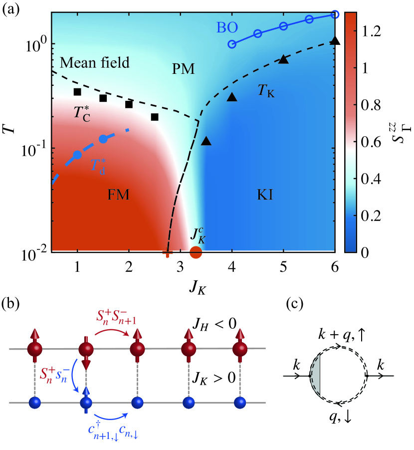
Figure 1: (a) The finite-temperature phase diagram of FMKH model. The contour background is the spin structure factor $S^{zz}_{k=\Gamma}$. The black dashed line is the phase boundary obtained by mean-field calculations which separates the paramagnetic (PM), ferromagnetic (FM) and Kondo insulator (KI) phase. In the ground state, the FM and KI phases are separated by a QCP at $J_{K}^{c}/|J_{H}|\approx 3.3$ indicated by the red circle obtained by DMRG, and the mean-field result shows a transition point at $\tilde{J}_{K}^{c}/|J_{H}|\approx 2.75$. The solid squares ($T_{\rm C}^{*}$) and triangles ($T_{\rm K}$) are obtained by TRG. The blue hollow circle of $T_{\rm K}$ is obtained from the bond operator (BO) theory. $T_{\rm d}^{*}$ in the FM phase represents the characteristic temperature with the damping rate minimum. (b) Magnon damping mechanism. The spin flip dissipates into the itinerant electron host through the Kondo coupling. (c) Feynman diagram of magnon self-energy due to electron-magnon scattering with the renormalized vertex responsible for the anomalous decay of magnon, where the double-dashed lines represent electron’s full propagator.

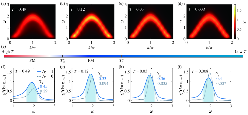
Figure 2: (a-d) show the contour plots of spectral density $\chi^{\prime\prime}$ at various temperatures computed in the $N=16\times 2$ system and with a retained bond dimension $D=1600$, and (e) shows the corresponding phase diagram. (f-i) show the comparisons of $\chi^{\prime\prime}(k=\pi,\omega)$ between the Heisenberg case ($J_{K}=0$, calculated by ED) and Kondo-Heisenberg case ($J_{K}=1$, $D=4800$). The fitted damping rate $\gamma_{\pi}$ is shown beside the peak (blue for Kondo-Heisenberg case and gray for pure Heisenberg case).

In Fig. 1(a) we show the obtained phase diagram of the FMKH model, with the contour plot of the spin structure factor $S^{zz}_{k}=\frac{1}{L}\sum_{m,n}\langle S_{m}^{z}S_{n}^{z}\rangle e^{{\rm i}(n-m)k}$ at $k=0$ (i.e., $\Gamma$ point) shown in the background. In the phase diagram we can recognize the existence of a ferromagnetic (FM, red) and a Kondo insulator (KI, blue) phase. At zero temperature, the two phases are separated by a quantum critical point (QCP), from which emanating the quantum critical regime at low temperature. The QCP located at $J_{K}^{c}\simeq 3.3$ is determined by the DMRG calculations, where we find an algebraic specific heat at low $T$ [40]. As temperature elevates, the FM and KI phases evolve into the high-temperature paramagnetic (PM) regime.

In companion with TRG numerics, we also perform mean-field calculations. By introducing the FM order parameter $m_{c}=\expectationvalue{s_{n}^{z}}$ and $m_{f}=\expectationvalue{S_{n}^{z}}$ and the Kondo hybridization order parameter [47, 48, 49] $V=\expectationvalue{c^{\dagger}_{n\uparrow}f_{n\uparrow}+f^{\dagger}_{n\downarrow}c_{n\downarrow}}$, where $f_{n,\sigma}$ is the pseudo-fermion operator for the local moment and $V$ characterizes the KI phase, we treat the FM and KI phases on an equal footing. The original Hamiltonian is then decoupled into a mean-field one that can be solved self-consistently [40]. The resulting phase boundary shown by the black dashed line in Fig. 1(a) is found to be in qualitative agreement with the TRG results. This is witnessed by the nice agreement between the mean-field dashed lines with the scatters ($T_{\rm C}^{*}$ and $T_{\rm K}$) determined from the peak location of the temperature derivatives of local moment correlations $-{dF_{nn}}/{dT}$ (with $F_{nn}=\frac{1}{L-1}\sum_{n}\langle{\boldsymbol{S}}_{n}\cdot{\boldsymbol{S}}_{n+1}\rangle$) and the local Kondo correlations $-{dK_{nn}}/{dT}$ (with $K_{nn}=-\frac{1}{L}\sum_{n}\langle{\boldsymbol{S}}_{n}\cdot{\boldsymbol{s}}_{n}\rangle$) [40]. In Fig. 1(a), we also represent the phase boundary determined by bond operator theory in KI phase as the blue circle  [40, 50, 51, 52], where qualitative agreements are also observed.

Damping rate minimum and logarithmic scaling.— Given the MPO representation of the thermal density matrix $\rho(\beta)=e^{-\beta H}$ ($\beta\equiv 1/T$), the dynamical properties at temperature $T$ can be simulated through a successive real-time evolution. The spectral function $\chi^{\prime\prime}(k,\omega)\approx\int_{0}^{t_{\rm max}}dt~{}{\rm Im}[g(k,t)]\sin{(\omega t)}\cdot W({t}/{t_{\rm max}})$ is of central interest in studying the dynamical properties at finite temperature, where $W$ is the window function, $t_{\rm max}$ is the evolution time, and the (dynamical) correlation function is $g(k,t)=\langle A_{k}(t)A_{k}^{\dagger}\rangle_{\beta}$, with $A_{k}=\frac{1}{\sqrt{L}}\sum_{n}^{L}S_{n}^{+}e^{{\rm i}kn}$ the Fourier transformed spin operator. Therefore, the problem resorts to the calculations of time-dependent correlation function $g(k,t)$, which we exploit the tangent-space approach to compute [37, 38, 39]. In the real-time evolution calculations, we consider a $16\times 2$ lattice and evolution time up to $t_{\rm max}/|J_{H}|=20$, with $D=4800$ bond states retained (see the data convergence in the Supplemental Sec. I C  [40]).

In Fig. 2(a-d), we show the spectral function $\chi^{\prime\prime}(\pi,\omega)$ of the FMKH model ($J_{K}=1$) where the line width firstly decreases and reaches its minimum at around $T^{*}_{\rm d}$, while it becomes broadened again as $T$ further lowers [c.f., the mini phase diagram Fig. 2(e)]. This is in sharp contrast to the pure Heisenberg ($J_{K}=0$) case where the line width narrows monotonically as temperature decreases and shows a very clear dispersion at low $T$ [40].

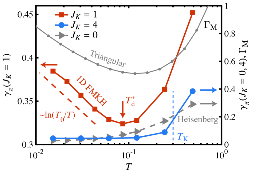
Figure 3: Damping rate $\gamma_{\pi}$ for the FMKH model in the FM ($J_{K}=1$) phase, as compared to that in the KI ($J_{K}=4$) phases and in pure Heisenberg model ($J_{K}=0$). In the FM phase of 1D FMKH model, the damping rate exhibits a minimum at the characteristic temperature $T_{\rm d}^{*}$, and below $T_{\rm d}^{*}$ it shows a logarithmic scaling $\gamma_{\pi}\sim\ln(T_{0}/T)$ with $T_{0}\simeq 0.27$. The gray solid line ($\Gamma_{\rm M}$) is the damping rate of triangular-lattice FMKH with $k={\rm M}\equiv(0,\frac{\sqrt{3}}{3}\pi)$, $J_{H}=-1$, $t=2$, and $J_{K}=10$ obtained via field-theoretical calculations (c.f. Supplemental Sec. III C [40]). In contrast, the spin excitations become more coherent as $T$ lowers for either the Heisenberg or the KI case. The vertical blue dashed line shows the Kondo temperature $T_{\rm K}\simeq 0.3$ of the KI phase, as estimated in Fig. 1(a).

It can be seen more clearly by plotting the $\chi^{\prime\prime}$ vs. $\omega$ at fixed $k=\pi$ [c.f., Fig. 2(f-i)], and compare the results to the pure Heisenberg ferromagnet. For the latter case, we find from the $\chi^{\prime\prime}(\omega)$ data that a more coherent peak develops as temperature lowers (i.e., absence of damping minimum); while for the $J_{K}=1$ case Kondo couplings introduce hybridization between local moments and the itinerant electron. With the spectral density results at $k=\pi$, we conduct a fitting with damped harmonic oscillator model [53], namely, $\chi^{\prime\prime}(k,\omega)\propto\frac{\gamma_{k}\omega E_{k}}{(\omega^{2}-E_{k}^{2})^{2}+(\gamma_{k}\omega)^{2}}\ast W(\omega)$ where $E_{k}$ is the magnon energy, $\gamma_{k}$ is the damping rate, and $W(\omega)$ is the convolution window function (c.f. Supplemental Sec. II B [40]). Based on the fittings of spectral density at $k=\pi$ in Fig. 2(f-h), we collect the fitted damping rate $\gamma_{\pi}$ and show the results in Fig. 3, where $\gamma_{\pi}$ clearly exhibits a damping minimum at $T_{\rm d}^{*}$. Remarkably, the numerical simulations find a logarithmic scaling $\gamma_{\pi}(T)\sim\ln{T_{0}/T}$ below $T_{\rm d}^{*}$. Such a damping minimum and logarithmic scaling can be observed in various momentum $k$ and for different Kondo couplings $J_{K}<J_{K}^{c}$, i.e., it is a universal behavior due to the scattering between the collective excitations (magnons) of local moments and itinerant electrons (c.f. Supplemental Sec. II C [40]).

As comparisons, we also show the damping rate $\gamma_{\pi}$ of the pure Heisenberg model ($J_{K}=0$) and that in the gapped KI phase with $J_{K}>J_{K}^{c}$ [54]. As shown in Fig. 3, for either the pure Heisenberg or the KI case, $\gamma_{\pi}$ decreases monotonically as $T$ lowers and converges to a small value (i.e., long life time). In the KI phase, the local moments and the itinerant electrons form a singlet and the triplon wave moves coherently without scattering the electrons, as verified both by numerics (c.f., Supplemental Sec. II E [40]) and the bond-operator theory [50, 51, 52] (c.f., Supplemental Sec. V [40]). Overall, the sharp contrasts in Fig. 3 reveal the peculiarity in the magnon damping minimum and logarithmic scaling, which roots deeply in the Kondo physics.

Field-theoretical analysis of the magnon decay.— We now provide a physical picture to explain this anomalous magnon decay based on a field-theoretical analysis. In the weak-coupling limit, $J_{K}\ll|J_{H}|,t$, the spin part and fermion part can be dealt with separately first. The former, via the Holstein-Primakoff mapping $S_{i}^{z}=S-n_{i}^{a}$ and $S_{i}^{+}\approx\sqrt{2S}a_{i}$, can be approximated by free magnons; while the latter is simply the free fermions. In this same representation, the Kondo coupling term, treated as a small perturbation, approximately reads $J_{K}\sum_{n}{\boldsymbol{S}}_{n}\cdot{\boldsymbol{s}}_{n}\approx\frac{J_{K}}{2}\sum_{i}(a_{i}c^{\dagger}_{i\downarrow}c_{i\uparrow}+\mathrm{H.c.})$ . Thus the magnon self-energy, according to the Dyson equation [56], is given diagrammatically in Fig. 1(c). In sharp contrast to the usual electron-phonon interaction where the vertex correction is negligible due to Migdal theorem [57], here the vertex correction [shown as a gray area in Fig. 1(c)] due to the Kondo coupling $J_{K}$ is crucial [19]. By incorporating this renormalization effect into the calculation of the magnon self-energy, a $\log(1/T)$-like temperature dependence of self-energy at low-$T$ is manifested (c.f. Supplemental Sec. III A [40]). In Fig. 3, for triangular-lattice model we incorporate magnon-magnon interactions that leads to a power-law divergence also at high-$T$, and find the magnon damping rate, proportional to the imaginary part of the self-energy therefore exhibits a minimum at an intermediate temperature and a logarithmic scaling at low temperatures [c.f. more details in Supplemental Sec. III C [40]].

Moreover, in Fig. 4(a-b), we show imaginary part of the renormalized magnon self-energy (omitting magnon-magnon interactions for simplicity) at relatively high ($T=0.1$) and low ($T=0.01$) temperatures, where $-\imaginary(\Sigma)$ increases as temperature lowers. We also plot the free magnon dispersion as the gray dash-dotted lines, whose large $|\boldsymbol{k}|$ part is found to “merge” into the regime of large $-\imaginary(\Sigma)$ values. Consequently, in Fig. 4(c-d) we find the corresponding renormalized magnon spectral density $\chi^{\prime\prime}(\omega)=-\imaginary[G_{k}({\rm i}\omega_{n}\rightarrow\omega+{\rm i}0^{+})]$ suffers heavier damping effect near the Brillouin zone boundary. This property, which is in agreement with recent INS experiments [18] and also shared by other lattice geometries, has a kinematic origin — There are many more damping channels for large $|\boldsymbol{k}|$. In Fig. 4(c-d), we plot the magnon spectral density at these two temperatures, and indeed find the dispersions get more blurred at a lower temperature $T=0.01$.

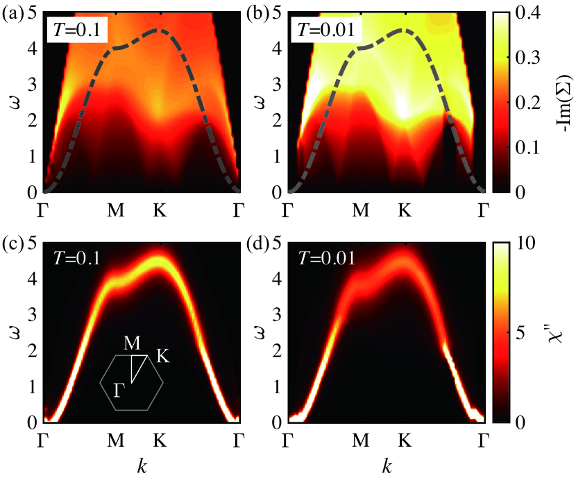
Figure 4: (a, b) the contour plot of the magnon self-energy $-{\rm Im}(\Sigma)$ of the triangular-lattice FMKH model at various temperatures, where the gray dashed lines are the free magnon dispersion. The spectral density $\chi^{\prime\prime}$ is shown in (c) and (d), with the $k$-path in the 1st Brillouin zone shown in the inset. Other parameters used: $t=1$, $J_{H}=-1$ and $J_{K}=1$.

Discussion and Outlook.— In this work, we study the finite-temperature dynamics of FMKH model with TRG calculations for 1D chain, with conclusions further supported by field-theoretical analysis for 2D lattice. A magnon damping minimum and universal logarithmic scaling at low temperature are revealed, which are ascribed to the scatterings between magnons and the itinerant electrons via the Kondo coupling. The logarithmical divergence of the effective Kondo coupling in the renormalization process (i.e., vertex correction) is analogous to the renowned Kondo effect. Our results well explain, from a theoretical point of view, the INS measurements on FGT [10, 18].

Based on the 1D model calculations, we uncover a QCP [58, 21, 43, 22] occurring at $J_{K}^{c}\simeq 3.3$ between the FM and KI phases in the phase diagram. We note in a recent experiment the Curie temperature of FGT compound decreases from $T_{\rm c}\simeq 200$ K to 100 K as pressure increases, with local moments also prominently suppressed [59]. The high sensitivity of Curie temperature of the FM order in FGT upon compression is consistent with present FMKH model study. Further experimental investigations on the pressurized FGT are thus called for according to our theoretical study here.

Supplemental Materials:
Magnon Damping Minimum and Logarithmic Scaling in a Kondo-Heisenberg Ferromagnet

Gao et al.

I Calculations of the Dynamical Properties of the Kondo-Heisenberg Model

I.1 Finite-temperature method: Exponential tensor renormalization group

The local Hilbert space of a fermion lattice site contains 4 states: the double occupied state $\ket{\uparrow\downarrow}$, single-occupied states $\ket{\uparrow},\ket{\downarrow}$, and the empty site $\ket{0}$. Consider a Kondo-Heisenberg lattice model described by Eq. 1 in the main text, the double occupied state $\ket{\uparrow\downarrow}$ and empty site $\ket{0}$ of the spin (local moment) sites are projected out (c.f., Fig. S1). To be specific, the Hilbert space is generated by the basis $(\{\ket{\uparrow},\ket{\downarrow}\}_{s}\otimes\{\ket{\uparrow\downarrow},\ket{\uparrow},\ket{\downarrow},\ket{0}\}_{f})^{\otimes N/2}$ where $s$ labels the spin (local moment) site while $f$ labels the fermion site, $N$ is the total number of spin and fermion sites. The matrix product operator (MPO) representation of the Hamiltonian is shown in Fig. S1.

We perform exponential tensor renormalization group (XTRG) simulations [27] of the finite-temperature properties, and to generate the finite-temperature density matrix for real-time simulations. In practical calculations, we start from the initial density matrix $\rho_{0}(\tau)$ of a very high temperature with $\tau=\mathcal{O}(10^{-4})$ ($T\equiv 1/\tau$), represented in a MPO form via a series expansion [26]

$$\rho_{0}(\tau)=e^{-\tau H}=\sum_{n=0}^{\infty}\frac{(-\tau H)^{n}}{n!}\simeq\sum_{n=0}^{N_{\rm cut}}\frac{(-\tau H)^{n}}{n!}.$$ (S1)

For a high temperature such as $\tau=2.5\times 10^{-4}$, the series expansion saturates to machine precision with cutoff $N_{\rm cut}=6$-$7$. Subsequently, by keeping squaring the density matrix repeatedly, i.e., $\rho_{n}(2^{n}\tau)\cdot\rho_{n}(2^{n}\tau)\to\rho_{n+1}(2^{n+1}\tau)$, we cool down the system along a logarithmic inverse-temperature grid $\tau\to 2\tau\to 2^{2}\tau\to...\to 2^{n}\tau$. Such a cooling process reaches low temperature exponentially fast, and it reduces significantly the projection and truncation steps, rendering higher accuracy than traditional linear evolution scheme, and thus it constitutes a very powerful thermal tensor network method for ultra-low temperature simulations.

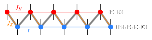
Figure S1: The MPO representation of the Kondo-Heisenberg model Hamiltonian. The red and blue sites present the spin and fermion site respectively with the corresponding local basis $\{\ket{\uparrow},\ket{\downarrow}\}$ and $\{\ket{\uparrow\downarrow},\ket{\uparrow},\ket{\downarrow},\ket{0}\}$. The red, blue and orange solid line represent the ferromagnetic exchange, hopping amplitude, and the Kondo coupling, respectively. The zigzag gray line shows the mapping between the ladder lattice and the MPO representation.

I.2 Real-time Evolution: TDVP for matrix product density operator

In Heisenberg picture, the real-time evolution of a given operator $\mathcal{O}$ reads $\mathcal{O}(t)=e^{{\rm i}Ht}\mathcal{O}_{0}e^{-{\rm i}Ht}$ with the corresponding Heisenberg equation

$${\rm i}\frac{d}{dt}\mathcal{O}=-[H,\mathcal{O}]=\mathcal{O}H-H\mathcal{O}.$$ (S2)

In practice, we introduce an auxiliary parameter $t^{\prime}$ such that $\mathcal{O}(t,t^{\prime})=e^{{\rm i}Ht}\mathcal{O}_{0}e^{-{\rm i}Ht^{\prime}}$, thus we can split Eq. S2 into two part, namely

$${\rm i}\frac{d}{dt}\mathcal{O} =-H\mathcal{O},$$ (S3a)

$${\rm i}\frac{d}{dt^{\prime}}\mathcal{O} =\mathcal{O}H.$$ (S3b)

In the tensor-network language, we prepare the operator $\mathcal{O}$ and the Hamiltonian $H$ in the MPO form. And Eq. S3 can be solved by the time-dependent variational principle (TDVP) [37, 38, 39] by introducing a Choi transformation [60]

$${\rm i}\frac{d}{dt}|\mathcal{O}\rangle\rangle =-H\otimes{I}|\mathcal{O}\rangle\rangle,$$ (S4a)

$${\rm i}\frac{d}{dt^{\prime}}|\mathcal{O}\rangle\rangle ={I}\otimes H^{\rm T}|\mathcal{O}\rangle\rangle.$$ (S4b)

Noticing that $e^{{\rm i}tH\otimes I}=e^{{\rm i}tH}\otimes I$ and $e^{-{\rm i}t^{\prime}I\otimes H}=I\otimes e^{-{\rm i}t^{\prime}H}$, we can solve Eq. S3 keeping the MPO form [28].

In this article, we consider the correlation function $g(k,t)$ calculated at temperature $\beta\equiv 1/T$, i.e.,

$$g(k,t)=\langle A_{k}(t)A_{k}^{\dagger}\rangle_{\beta}=\frac{1}{Z}{\rm tr}[e^{{\rm i}Ht}e^{-\frac{\beta}{2}H}A_{k}e^{-{\rm i}Ht}A_{k}^{\dagger}e^{-\frac{\beta}{2}H}],$$ (S5)

where $Z$ is the partition function and

$$A_{k}=\frac{1}{\sqrt{L}}\sum_{n=1}^{L}S_{n}^{+}e^{{\rm i}kn},\quad k=\frac{2\pi m}{L},\quad m\in\{0,1,\cdots,L-1\}$$ (S6)

With the density matrix at inverse temperature ${\beta}/{2}$, the correlation function $g(k,t)$ can be obtained by performing real-time evolution of $e^{-\frac{\beta}{2}H}A_{k}$ following Fig. S2. In the present work, we perform calculations with retained bond dimension up to $4800$, $\delta t=0.1$, and $t_{\rm max}=20$.

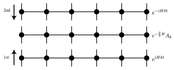
Figure S2: The workflow of real-time evolution with a small step $\delta t$, starting form the quenched finite temperature density matrix $e^{-\frac{\beta}{2}H}A_{k}$. The evolution operator $e^{{\rm i}H\delta t}$ and $e^{{-\rm i}H\delta t}$ are acted on $e^{-\frac{\beta}{2}H}A_{k}$ following the order indicated by the arrows.

I.3 Data convergence for real-time evolution

In Fig. S3, we show the real-time evolutions versus different bond dimension $D$, where we find the simulated results have reached convergence for $D\gtrsim 4000$.

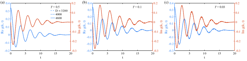
Figure S3: Real (blue) and imaginary (red) part of the real-time correlation function with different bond dimensions for (a) $T=0.5$, (b) $T=0.1$, and (c) $T=0.03$. The system size is $N=16\times 2$, the hopping amplitude is $t=2$, the Heisenberg exchange is $J_{H}=-1$ and the Kondo coupling $J_{K}=1$.

II Additional Data of the Spectral Density

II.1 Calculations of the spectral density

The spectral function in a time translation invariant system is defined as $\chi_{AB}^{\prime\prime}(t)=\frac{1}{2\pi}\langle[A(t),B]\rangle$ and below we consider the spin excitation in the FMKH model, with $A=S^{+}$ and $B=A^{\dagger}=S^{-}$. The correlation function $g(k,t)$ is defined as

$$g(k,t)=\langle S^{+}_{k}(t)S_{k}^{-}\rangle_{\beta}=\frac{1}{Z}{\rm tr}[e^{{\rm i}Ht}e^{-\frac{\beta}{2}H}S^{+}_{k}e^{-{\rm i}Ht}S_{k}^{-}e^{-\frac{\beta}{2}H}]=g(k,-t)^{\ast}.$$ (S7)

Due to the spatial inversion symmetry, $g(k,t)=g(-k,t)$. Moreover, we have $\langle S^{+}(t)S^{-}\rangle_{\beta}=\langle S^{-}(t)S^{+}\rangle_{\beta}$ for the present system. Thus the spectral density reads

$$\chi^{\prime\prime}(k,t)=\frac{1}{2\pi}[g(k,t)-g(k,t)^{*}]=\frac{{\rm i}}{\pi}{\rm Im}~{}g(k,t),$$ (S8)

and

$$\chi^{\prime\prime}_{\rm def}(k,\omega)\equiv\int_{-\infty}^{+\infty}dt~{}e^{{\rm i}t\omega}\frac{{\rm i}}{\pi}{\rm Im}~{}g(k,t)=-\frac{2}{\pi}\int_{0}^{\infty}dt~{}{\rm Im}~{}g(k,t)\sin\omega t.$$ (S9)

Since the real-time simulation can only be performed for a finite period of time, the spectral function can be obtained approximately as

$$\chi^{\prime\prime}(k,\omega)\approx-a\int_{0}^{t_{\rm max}}dt~{}{\rm Im}~{}g(k,t)\sin\omega t\cdot W(\frac{t}{t_{\rm max}}),$$ (S10)

where $W(t)$ is a window function, and $a$ is a nonsignificant constant number (we set $a=1$ in the follow part). In practice, the Hanning window defined below is chosen,

$$W(t)=\begin{cases}\frac{1}{2}+\frac{1}{2}\cos(\pi t),&|t|\leq 1\\ 0,&|t|>1.\end{cases}$$ (S11)

II.2 Kondo-Heisenberg model and the damped harmonic oscillator analysis

We fit $\chi^{\prime\prime}$ by the damped harmonic oscillator (DHO) model defined as [53]

$$\chi^{\prime\prime}_{\rm def}(k,\omega)\propto\frac{\gamma_{k}\omega E_{k}}{(\omega^{2}-E_{k}^{2})^{2}+(\gamma_{k}\omega)^{2}}$$ (S12)

where $E_{k}$ is the magnon energy and $\gamma_{k}$ is the damping rate. Since the time window of real-time evolution is limited by tensor network calculations, we add a Hanning window for cut-off. In practice, the DHO fitting should take into account of the influences from the window.

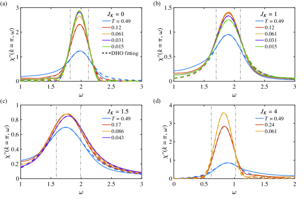
Figure S4: The DHO fittings of $\chi^{\prime\prime}(k,\omega)$ results of (a) Heisenberg model with Kondo coupling $J_{K}=0$ (ED), (b) $J_{K}=1$ ($D=4800$), (c) $J_{K}=1.5$ ($D=3200$), and (d) $J_{K}=4$ ($D=1600$). The solid lines are the calculated $\chi^{\prime\prime}(k,\omega)$ results at different temperatures, and the correspond DHO fittings are shown with dashed lines and in the same color code. The fitting window is indicated by the two gray lines. In (a) for the Heisenberg ferromagnet with $J_{K}=0$, we take $J_{H}=-1$ and the calculations are performed on a $L=16$ chain. For the $J_{K}>0$ cases in (b,c,d) panels, instead we take $t=2$, $J_{H}=-1$ and the system size is $N=16\times 2$.

From Eq. S10, one may immediately find that

$$\chi^{\prime\prime}(\omega)=\frac{1}{2\pi}\chi^{\prime\prime}_{\rm def}(\omega)\ast W(\omega).$$ (S13)

Thus the DHO fitting is

$$\chi^{\prime\prime}(\omega)\propto\frac{\gamma_{k}\omega E_{k}}{(\omega^{2}-E_{k}^{2})^{2}+(\gamma_{k}\omega)^{2}}\ast W(\omega),$$ (S14)

where $W(\omega)=\frac{\pi^{2}\sin(t_{\rm max}\omega)}{-\pi^{2}\omega+t_{\rm max}\omega^{3}}$ is the fourier transform of Hanning window.

The DHO fitting results are shown in Fig. S4 with the $\chi^{\prime\prime}(k,\omega)$ obtained by TDVP ($J_{K}>0$) and exact diagonalization ($J_{K}=0$). Within the fitting range, i.e. the gray line in Fig. S4, the DHO fitting shows excellent agreement with $\chi^{\prime\prime}(k,\omega)$.

II.3 Damping rate minima and logarithmic scaling for different $J_{K}$

The damping minimum and the logarithmic scaling can also be obtained with different momentum $k$ and Kondo coupling $J_{K}$ as shown in Fig. S5. Since the damping coefficient is related to the magnon self-energy ${\rm Im}(\Sigma)$, the momentum $k<1$ is lesser influenced by the Kondo effect, i.e., the damping minimum is reached with a smaller temperature [see Fig. S5 (a)]. For $J_{K}=1.5$, we obtained the damping coefficient with $N=16\times 2$ and $D=3200$. As shown in Fig. S5 (b), $\gamma_{\pi}$ shows similar behavior to the main text case. Increasing $J_{K}$, $T_{\rm d}^{*}$ also becomes higher.

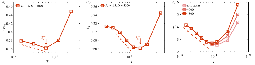
Figure S5: Supporting data of the damping coefficient $\gamma_{k}$ for more coupling parameter $J_{K}$ and momentum $k$. (a) $J_{K}=1$ ($k=4\pi/3$) and (b) $J_{K}=1.5$ ($k=\pi$), simulated on a $N=16\times 2$ geometry. $T_{\rm d}^{*}$ indicates the damping minimum of $\gamma_{k}$ and the dashed line represents the logarithmic scaling. (c) shows the rescaled damping coefficient $\gamma^{\prime}_{\pi}$ with different bond dimension $D$, where the logarithmic scaling is found to be robust for various $D$.

To confirm the low-temperature scaling of the damping constant, we fit the damping coefficient $\gamma_{\pi}$ under different retaining bond dimension by the model $a\log(b/T)+c$. The rescaled damping coefficient $\gamma^{\prime}_{\pi}=\frac{1}{a}(\gamma_{\pi}-c)-\log(b)$ is shown in Fig. S5(c), and the low-temperature part shows exactly same behavior.

II.4 Ferromagnetic Heisenberg chain: ED calculations

As for the pure Heisenberg case ($J_{K}=0$) with $L=16$, we obtain the dynamical properties by exact diagonalization (ED) calculations. The contour plots of the spectral density are shown in Fig. S6, where the dispersion line shape becomes clearer as temperature lowers.

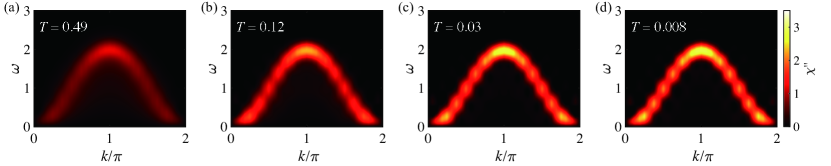
Figure S6: Contour plot of spectral density $\chi^{\prime\prime}$ of a pure FM Heisenberg chain with $L=16$ at various temperatures.

II.5 Coherent triplon excitations in the Kondo insulator phase

For sufficiently large Kondo coupling $J_{K}$, the system enters the Kondo insulator phase with coherent triplon waves. As shown in Fig. S7, we calculate the spin excitation dispersions with tensor network approach, and find the triplon excitation shows a square form dispersion with a minimum value at $k/\pi=1$.

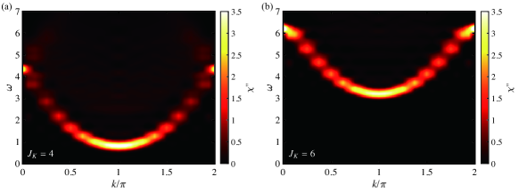
Figure S7: Triplon dispersion for (a) $J_{K}=4$ and (b) $J_{K}=6$, with $D=1600$, $N=16\times 2$ and $T=0.03$.

III Field Theoretical Analysis of the Magnon Damping Rate

III.1 Explicit evaluation of the bare polarization bubble diagram for the 1D chain

The pair bubble diagram for the magnon self-energy, given in Fig. 1(c), using bare electron propagator and bare vertex, reads

$$\Sigma_{\boldsymbol{k}}({\rm i}\omega_{n}) =\Sigma^{+-}_{\boldsymbol{k}}({\rm i}\omega_{n})$$

$$=\leavevmode\hbox to40.23pt{\vbox to22.59pt{\text{[drawing]}}}$$

$$=-\frac{J_{K}^{2}}{2}\int\frac{\mathrm{d}^{d}p}{(2\pi)^{d}}\frac{n_{c,\boldsymbol{p}+\boldsymbol{k}}-n_{c,\boldsymbol{p}}}{{\rm i}\omega_{n}-\epsilon_{c,\boldsymbol{p}+\boldsymbol{k}}+\epsilon_{c,\boldsymbol{p}}},$$ (S15)

where $n_{c,\boldsymbol{k}}=1/(e^{\beta\epsilon_{c,\boldsymbol{k}}}+1)$ is the Fermi function. For the 1D chain, after analytical continuation, ${\rm i}\omega_{n}\rightarrow\omega+{\rm i}0^{+}$, we have

$$\Sigma_{k}(\omega+{\rm i}0^{+}) =-\frac{J_{K}^{2}}{2}\int\frac{dp}{2\pi}\frac{n_{c,p+k}-n_{c,p}}{\omega-\epsilon_{c,p+k}+\epsilon_{c,p}+i0^{+}}$$

$$=-\frac{J_{K}^{2}}{2}\int\frac{dp}{2\pi}\frac{n_{c,p+k}-n_{c,p}}{\omega-\epsilon_{c,p+k}+\epsilon_{c,p}}+{\rm i}\bigg{[}\frac{\pi J_{K}^{2}}{2}\int\frac{dp}{2\pi}(n_{c,p+k}-n_{c,p})\delta(\omega-\epsilon_{c,p+k}+\epsilon_{c,p})\bigg{]}.$$ (S16)

From

$$\chi_{k}^{\prime\prime}(\omega) =-\imaginary[G^{R}_{k}(\omega+{\rm i}0^{+})]$$

$$=-\imaginary\frac{1}{\omega-E_{k}-\real\Sigma_{k}(\omega)-{\rm i}\imaginary\Sigma_{k}(\omega)}$$

$$=\frac{-\imaginary\Sigma_{k}(\omega)}{[\omega-E_{k}-\real\Sigma_{k}(\omega)]^{2}+[\imaginary\Sigma_{k}(\omega)]^{2}},$$ (S17)

the magnon damping rate is found to be

$$\gamma(\omega,k) =\absolutevalue{\imaginary\Sigma_{k}(\omega)}$$

$$=\absolutevalue{\frac{\pi K^{2}}{2}\int\frac{dp}{2\pi}(n_{c,p+k}-n_{c,p})\delta(\omega-\epsilon_{c,p+k}+\epsilon_{c,p})}$$

$$=\frac{J_{K}^{2}}{8t}\sum_{p_{0}}\absolutevalue{\frac{n_{c,p_{0}+k}-n_{c,p_{0}}}{\sin(p_{0}+k)-\sin p_{0}}}$$

$$=\frac{J_{K}^{2}}{16t}\sum_{p_{0}}\absolutevalue{\frac{n_{c,p_{0}+k}-n_{c,p_{0}}}{\cos\frac{2p_{0}+k}{2}\sin\frac{k}{2}}},$$ (S18)

where the summation runs over all solutions of the following equation for $p_{0}\in[-\pi,\pi)$,

$$\omega =\epsilon_{c,p_{0}+k}-\epsilon_{c,p_{0}}$$

$$=4t\sin\frac{2p_{0}+k}{2}\sin\frac{k}{2}.$$ (S19)

where $\epsilon_{c,k}=-2t\cos k$ is the dispersion of free fermion chain. Focusing on the on-shell region, $\omega=\epsilon_{k}=\absolutevalue{J_{H}}(1-\cos k)$, Eq. (S19) always has two solutions given by $p_{0,1}=-\frac{k}{2}+\arccsc\bqty{\alpha\csc\frac{k}{2}}$ and $p_{0,2}=-\frac{k}{2}+\pi-\arccsc\bqty{\alpha\csc\frac{k}{2}}$ with $\alpha=2t/|J_{H}|>1$ for the model parameters of Fe₃GeTe₂. Limiting cases of the bare damping rate can be understood from the analytical expression Eq. (S18). First, it is vanishingly small for small $k$. Indeed, when expanded around $k=0$, it’s straightforward to show that $\gamma\propto k$. Secondly, it should reach the maximal value for $k$ near $\pi$, where the numerator becomes largest. Lastly, to the crudest approximation and as a reminiscence of the single-impurity Kondo problem, the Kondo coupling $J_{K}$ is renormalized as $J_{K}\rightarrow J_{K}^{\rm ren}=J_{K}[1+J_{K}g(\epsilon_{F})\log(\frac{\Lambda}{T})]$, where $g(\epsilon_{F})=1/(2\pi t)$ is the density of states per spin at the Fermi energy, and $\Lambda=4t$ is the band width. When comparing with our numerical calculations given in Fig. 3, it is found that these model parameters should be further renormalized as $J_{H}=-0.07$ and $J_{K}=0.88$, which may be due to higher order corrections.

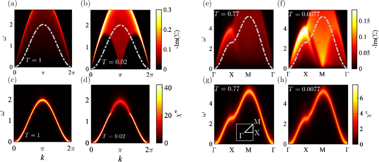
Figure S8: First row: Contour plot of the imaginary part of magnon self-energy $\imaginary(\Sigma)$ for the Kondo-Heisenberg lattice model defined on the one-dimensional chain (a-b) and the square lattice (e-f), where the gray dash-dotted line is the corresponding free magnon dispersion. Second row: the corresponding magnon spectral density $\chi^{\prime\prime}=\imaginary G^{R}$, for the one-dimensional chain (c-d) and the square lattice (g-h) cases. The inset in (g) shows the momentum path used in the first Brillouin zone. Parameters used: $t/|J_{H}|=0.81$ and $J_{K}/|J_{H}|=0.21$ for the one-dimensional chain case; $t/|J_{H}|=0.77$ and $J_{K}/|J_{H}|=0.077$ for the square lattice case.

We present numerical results of imaginary part of magnon self-energy in Fig. S8(a-b) and the corresponding spectral density in Fig. S8(c-d). It is found indeed that the imaginary part of the magnon self-energy increases at lower temperature and the magnon spectral density becomes more damped. Once again, we note that within this simple one-loop calculations, the magnon damping occurs only around $k\sim\pi$ and is absent for small $|k|$.

III.2 The square lattice case

For the FMKH model defined on the square lattice, with the primitive lattice vectors given by $\boldsymbol{u}_{1}=(1,0)$ and $\boldsymbol{u}_{2}=(0,1)$, the corresponding Brillouin zone is shown in the inset of Fig. S8(g). After using the Holstein-Primakoff transformation, the free magnon dispersion is $\epsilon_{\boldsymbol{k}}=J(2-\cos k_{x}-\cos k_{y})$. Meanwhile, the free electron dispersion reads $\epsilon_{c,\boldsymbol{k}}=-2t(\cos k_{x}+\cos k_{y})$. Hence the self-energy can be calculated numerically using Eq. (3) in the main text, and results are shown in Fig. S8. Note at half-filling, the density of state of free fermion for the square lattice is divergent due to the presence of van Hove singularity, which is of course an artifact resulting from the approximation used in calculating the corresponding momentum integration. In practice, we simply regularize this density of state to a finite one in comparable to the one-dimensional case. The two main features, which are also shared for the one-dimensional case and the triangular lattice case, are that (1) the imaginary part of magnon self-energy increases at lower temperature, and the corresponding magnon spectral density is more damped; (2) damping phenomenon occurs primarily at large $|\boldsymbol{k}|$ and becomes absent for small $|\boldsymbol{k}|$. The second feature can easily be understood from the kinematics: the damping channel becomes negligible for small $|\boldsymbol{k}|$, therefore the magnon remains to be well-defined in that case.

III.3 Magnon damping minimum for the triangular lattice case

The calculations present in this section so far only produce $\log T$ scaling of magnon damping at low temperature. While in experiment it is found that there is also a magnon damping minimum at an intermediate temperature [18]. In this subsection, we further consider magnon-magnon interactions beyond linear spin wave theory. It turns out that this additional contribution gives a power-law divergence at relatively high temperatures. Together with contributions from electron-magnon interactions, the magnon damping minimum found in experiments is therefore reproduced.

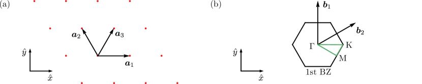
Figure S9: (a) The triangular lattice is generated by linear combinations of the basis vectors $\bm{a}_{1}=\pqty{1,0}$ and $\bm{a}_{2}=\pqty{-1/2,\sqrt{3}/2}$. (b) The corresponding reciprocal lattice is generated by the basis vectors $\bm{b}_{1}=2\pi\times(1,1/\sqrt{3})$ and $\bm{b}_{2}=2\pi\times(0,1/\sqrt{3})$. The first Brillouin zone (BZ) is shown as a hexagon, with the high symmetric path indicated by the green lines.

As the minimal model Hamiltonian for Fe₃GeTe₂, the ferromagnetic Kondo-Heisenberg model on the triangular lattice reads $H=H_{t}+H_{J}+H_{K}$, where

$$H_{t} =-t\sum_{\langle i,j\rangle}c^{\dagger}_{i,\sigma}c_{j,\sigma}+\text{H.c.},$$ (S20)

$$H_{J} =-J\sum_{\langle i,j\rangle}\bm{S}_{i}\cdot\bm{S}_{j},$$ (S21)

$$H_{K} =J_{K}\sum_{i}\bm{S}_{i}\cdot\bm{s}_{i}.$$ (S22)

Using the Holstein-Primakoff (HP) transformation,

$$S^{+}_{i} =\sqrt{2S-a^{\dagger}_{i}a_{i}}a_{i},$$ (S23a)

$$S^{-}_{i} =a^{\dagger}_{i}\sqrt{2S-a^{\dagger}_{i}a_{i}},$$ (S23b)

$$S^{z}_{i} =S-a^{\dagger}_{i}a_{i},$$ (S23c)

Equation (S21) can be rewritten as $H_{J}=H^{(-2)}+H^{(-1)}+H^{(0)}+\mathcal{O}\pqty{\frac{1}{S}}$. Here the superscript labels the corresponding order in $1/S$. Explicitly, we have

$$H^{(-2)} =\pqty{\frac{1}{S}}^{-2}\times(-zNJ),$$ (S24)

$$H^{(-1)} =\pqty{\frac{1}{S}}^{-1}\times 2zJ\sum_{\bm{k}}(1-\gamma_{\bm{k}})a^{\dagger}_{\bm{k}}a_{\bm{k}},$$ (S25)

$$H^{(0)} =\pqty{\frac{1}{S}}^{0}\times\frac{J}{4}\sum_{\langle i,j\rangle}\pqty{a^{\dagger}_{i}a^{\dagger}_{i}a_{i}a_{j}+a^{\dagger}_{j}a^{\dagger}_{j}a_{i}a_{j}+a^{\dagger}_{i}a^{\dagger}_{j}a_{i}a_{i}+a^{\dagger}_{i}a^{\dagger}_{j}a_{j}a_{j}-4a^{\dagger}_{i}a^{\dagger}_{j}a_{i}a_{j}}$$ (S26)

$$=\sum_{\{\bm{k}_{i}\}}{}^{{}^{\prime}}V_{4}(\bm{k}_{1},\bm{k}_{2};\bm{k}_{3},\bm{k}_{4})a^{\dagger}_{\bm{k}_{1}}a^{\dagger}_{\bm{k}_{2}}a_{\bm{k}_{3}}a_{\bm{k}_{4}}.$$ (S27)

Equation (S24) gives the classical ground state energy for a pure ferromagnetic Heisenberg model on the triangular lattice, with $z=3$ half the coordination number and $N$ the total lattice sites. Equation (S25) gives the free magnon dispersion $\varepsilon_{\bm{k}}=2zSJ(1-\gamma_{\bm{k}})$. For the triangular lattice, we have $\gamma_{\bm{k}}=\frac{1}{z}\sum_{l=1}^{z}\cos(\bm{a}_{l}\cdot\bm{k})$, with $\bm{a}_{1,2,3}$ shown in Fig. S9(a). Equation (S26) gives the interaction between magnons, where the interaction vertex explicitly reads $V_{4}(\bm{k}_{1},\bm{k}_{2};\bm{k}_{3},\bm{k}_{4})=\frac{J}{4N}\pqty{\gamma_{\bm{k}_{1}}+\gamma_{\bm{k}_{2}}+\gamma_{\bm{k}_{3}}+\gamma_{\bm{k}_{4}}-4\gamma_{\bm{k}_{2}-\bm{k}_{4}}}$. The primed summation in Eq. (S27) means that the total momentum before and after scattering is conserved, i.e., $\bm{k}_{1}+\bm{k}_{2}=\bm{k}_{3}+\bm{k}_{4}$. Using the same HP transformation, Equation (S22) can be written as

$$H=J_{K}\sum_{i}\bqty{(S-n_{i})(n^{f}_{i,\uparrow}-n^{f}_{i,\downarrow})+\sqrt{\frac{S}{2}}(a_{i}c^{\dagger}_{i,\downarrow}c_{i,\uparrow}+a^{\dagger}_{i}c^{\dagger}_{i,\uparrow}c_{i,\downarrow})}+\mathcal{O}\pqty{\pqty{{\frac{1}{S}}}^{1/2}}.$$ (S28)

Based on Eq. (S27) and (S28), all contributions to magnon self-energy up to the zeroth order in $1/S$ and second order in $J$ and $J_{K}$ are listed in Fig. S10.

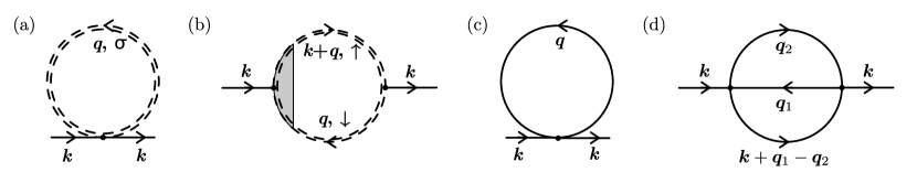
Figure S10: Contributions to magnon self-energy due to electron-magnon interaction [(a) and (b)] and magnon-magnon interaction (up to zeroth order in $1/S$ and second order in $J$) [(c) and (d)]. Solid (dashed double) line represents free magnon (renormalized electron) propagators. For simplicity, we replace the renormalized electron propagator by the bare one for all our calculations. The gray area in (b) indicates the usage of renormalized vertex. Here we also simply use the replacement $J_{K}\rightarrow J_{K}^{(\text{ren})}=J_{K}[1+J_{K}g(\epsilon_{F})\log(\frac{\Lambda}{T})]$, as in the case of single impurity Kondo model, which is responsible for the anomalous temperature dependence of magnon damping rate at low temperatures.

Figure S10(a) is a Hartree contribution, which vanishes since $\langle n^{f}_{i,\uparrow}\rangle_{0}=\langle n^{f}_{i,\downarrow}\rangle_{0}$. Namely,

$$\Sigma^{(a)}_{R}(\bm{k})=0.$$ (S29)

Figure S10(b) explicitly reads $\Sigma^{(b)}(\bm{k},i\omega)=J_{K}^{2}\frac{S}{2}\chi_{0}(\bm{k},i\omega)$, where the pair-bubble diagram is

$$\chi_{0}(\bm{k},i\omega) =\frac{1}{N}\sum_{\bm{q}}\frac{1}{\beta}\sum_{i\omega_{1}}\frac{1}{i\omega_{1}-\xi_{\bm{q}}}\frac{1}{i\omega+i\omega_{1}-\xi_{\bm{k}+\bm{q}}}$$ (S30)

$$=\frac{1}{N}\sum_{\bm{q}}\frac{f_{F}(\xi_{\bm{q}})-f_{F}(\xi_{\bm{k}+\bm{q}})}{i\omega-(\xi_{\bm{k}+\bm{q}}-\xi_{\bm{q}})},$$ (S31)

and $\xi_{\bm{k}}=-2tz\gamma_{\bm{k}}$ is free electron’s dispersion. After analytical continuation, and using renormalization of Kondo coupling $J_{K}\rightarrow J_{K}^{\text{(ren)}}=J_{K}[1+J_{K}g(\epsilon_{F})\log(\frac{\Lambda}{T})]$ reminiscent of the singlet-impurity Kondo problem [19], the retarded self-energy reads

$$\Sigma^{(b)}_{R}(\bm{k},\omega)=J_{K}^{2}\bqty{1+J_{K}g(\epsilon_{F})\log(\frac{\Lambda}{T})}\frac{S}{2N}\sum_{\bm{q}}\frac{f_{F}(\xi_{\bm{q}})-f_{F}(\xi_{\bm{k}+\bm{q}})}{\omega-(\xi_{\bm{k}+\bm{q}}-\xi_{\bm{q}})+i0^{+}}.$$ (S32)

Here $g(\epsilon_{F})$ is the density of states per spin at the Fermi energy, and $\Lambda$ is the band width.

Figure S10(c) is also a Hartree contribution. We replace the product of two operators by their expectation values in Eq. (S27), which leads to four non-vanishing terms. After simplification, the upshot is simply a correction to the magnon dispersion relation,

$$\Sigma^{(c)}_{R}(\bm{k})=\sum_{\bm{q}}2J(\gamma_{\bm{q}}+\gamma_{\bm{k}}-\gamma_{0}-\gamma_{\bm{k}-\bm{q}})f_{B}(\varepsilon_{\bm{q}}).$$ (S33)

Figure S10(d) explicitly reads

$$\Sigma^{(d)}(\bm{k},i\omega) =\frac{J^{2}}{N^{2}\beta^{2}}\sum_{\{\bm{q}_{i},i\omega_{i}\}}\frac{\absolutevalue{V_{4}(\bm{k},\bm{q}_{1};\bm{q}_{2},\bm{k}+\bm{q}_{1}-\bm{q}_{2})}^{2}}{(i\omega_{1}-\varepsilon_{\bm{q}_{2}})(i\omega_{2}-\varepsilon_{\bm{k}+\bm{q}_{1}-\bm{q}_{2}})[i(\omega_{1}+\omega_{2}-\omega)-\varepsilon_{\bm{q}_{1}}]}$$ (S34)

$$=\frac{J^{2}}{N^{2}}\sum_{\{\bm{q}_{i}\}}\frac{\absolutevalue{V_{4}(\bm{k},\bm{q}_{1};\bm{q}_{2},\bm{k}+\bm{q}_{1}-\bm{q}_{2})}^{2}}{i\omega+\varepsilon_{\bm{q}_{1}}-\varepsilon_{\bm{q}_{2}}-\varepsilon_{\bm{k}+\bm{q}_{1}-\bm{q}_{2}}}F_{\bm{k},\bm{q}_{1},\bm{q}_{2}}.$$ (S35)

where $F_{\bm{k},\bm{q}_{1},\bm{q}_{2}}=\bqty{1+f_{B}(\varepsilon_{\bm{q}_{2}})}\bqty{1+f_{B}(\varepsilon_{\bm{k}+\bm{q}_{1}-\bm{q}_{2}})}f_{B}(\varepsilon_{\bm{q}_{1}})-f_{B}(\varepsilon_{\bm{q}_{2}})f_{B}(\varepsilon_{\bm{k}+\bm{q}_{1}-\bm{q}_{2}})\bqty{1+f_{B}(\varepsilon_{\bm{q}_{1}})}$. After analytical continuation, the retarded self-energy reads

$$\Sigma^{(d)}_{R}(\bm{k},\omega)=\frac{J^{2}}{N^{2}}\sum_{\{\bm{q}_{i}\}}\frac{\absolutevalue{V_{4}(\bm{k},\bm{q}_{1};\bm{q}_{2},\bm{k}+\bm{q}_{1}-\bm{q}_{2})}^{2}}{\omega+\varepsilon_{\bm{q}_{1}}-\varepsilon_{\bm{q}_{2}}-\varepsilon_{\bm{k}+\bm{q}_{1}-\bm{q}_{2}}+i0^{+}}F_{\bm{k},\bm{q}_{1},\bm{q}_{2}}.$$ (S36)

Thus the total retarded self-energy reads $\Sigma_{R}=\Sigma_{R}^{(a)}+\Sigma_{R}^{(b)}+\Sigma_{R}^{(c)}+\Sigma_{R}^{(d)}$. And its imaginary part, relating to the magnon damping rate, reads

$$\Gamma(\bm{k},\omega) =\absolutevalue{\text{Im}\Sigma_{R}(\bm{k},\omega)}$$ (S37)

$$=\absolutevalue{\text{Im}\Sigma_{R}^{(b)}(\bm{k},\omega)+\text{Im}\Sigma_{R}^{(d)}(\bm{k},\omega)}$$ (S38)

$$=|J_{K}^{2}\bqty{1+J_{K}g(\epsilon_{F})\log(\frac{\Lambda}{T})}\frac{S\pi}{2N}\sum_{\bm{q}}\bqty{f_{F}(\xi_{\bm{q}})-f_{F}(\xi_{\bm{k}+\bm{q}})}\delta(\omega-(\xi_{\bm{k}+\bm{q}}-\xi_{\bm{q}}))$$

$$\quad+\frac{\pi J^{2}}{N^{2}}\sum_{\{\bm{q}_{i}\}}\absolutevalue{V_{4}(\bm{k},\bm{q}_{1};\bm{q}_{2},\bm{k}+\bm{q}_{1}-\bm{q}_{2})}^{2}F_{\bm{k},\bm{q}_{1},\bm{q}_{2}}\delta(\omega+\varepsilon_{\bm{q}_{1}}-\varepsilon_{\bm{q}_{2}}-\varepsilon_{\bm{k}+\bm{q}_{1}-\bm{q}_{2}})|.$$ (S39)

There are two contributions: one results from the Kondo coupling, $\Sigma^{(b)}_{R}$, and the other is due to magnon-magnon interactions, $\Sigma^{(d)}_{R}$. Each of them is an integration, and the corresponding integrand consists of two parts, the scattering coefficient and the delta function. The former gives temperature dependence and overall relative strength among different momenta; while the latter provides the kinematic constraint. To understand this kinematic constraint more carefully, we define the scattering density of states [61] for each contribution,

$$K^{(b)}(\bm{k}) =\frac{1}{N}\sum_{\bm{q}}\delta(\omega-(\xi_{\bm{k}+\bm{q}}-\xi_{\bm{q}})),$$ (S40)

$$K^{(d)}(\bm{k}) =\frac{1}{N^{2}}\sum_{\{\bm{q}_{i}\}}\delta(\omega+\varepsilon_{\bm{q}_{1}}-\varepsilon_{\bm{q}_{2}}-\varepsilon_{\bm{k}+\bm{q}_{1}-\bm{q}_{2}}).$$ (S41)

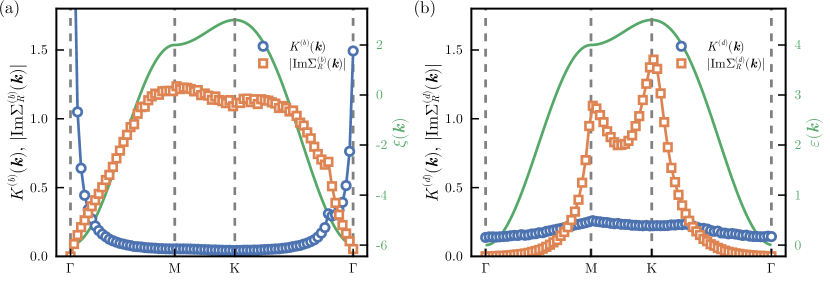
Figure S11: Scattering density of states $K$ and imaginary part of the self-energy $\text{Im}\Sigma$ due to (a) electron-magnon interactions and (b) magnon-magnon interactions, together with free electron dispersion $\xi(\bm{k})$ and free magnon dispersion $\varepsilon(\bm{k})$, respectively, along the high symmetry momentum path. Model parameters used: $t/J=1$, $J_{K}/J=10$ and $T=1$. Error bars of numerical integration are smaller than the symbol size.

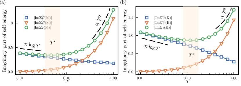
Figure S12: Imaginary part of the self-energy from two types of interactions and their total contributions (namely, the magnon damping rate), as a function of temperature $T$, at the M (a) and K (b) point in the first BZ. The shaded rectangle with $T^{\ast}$ indicates the regime where magnon damping minimum occurs. Model parameters used: $t/J=2$, $J_{K}/J=12$. Error bars of numerical integration are smaller than the symbol size.

In Fig. S11, we show the imaginary part of self-energy $\text{Im}\Sigma$ and the corresponding scattering density of states $K$, for each contribution. The multi-dimensional integrations over internal momenta are performed using MCIntegration.jl [62]. It is found that for the electron-magnon interactions, the scattering density of states is divergent around $\Gamma$ point and suppressed otherwise; while for the magnon-magnon interactions, it peaks at $M$ point and reaches minimum at $\Gamma$ and $K$. For the respective contributions to the magnon damping, namely the imaginary part of the self-energy, both become larger when going away from the BZ center, and become largest near the BZ boundary. This behavior is consistent with the experimental observation in Fe₃GeTe₂ [18].

In Fig. S12, we show the temperature dependence of the damping rate resulting from two types of interactions and their total contribution. In the large and small $T$ limit, imaginary part of Eq. (S32) and (S36) can be understood analytically: On the one hand, it can be shown straightforwardly that $\text{Im}\Sigma_{R}^{(b)}\propto 1/T$ for $T\rightarrow\infty$ and $\text{Im}\Sigma_{R}^{(d)}$ decay exponentially for $T\rightarrow 0$, respectively. On the other hand, $\text{Im}\Sigma_{R}^{(d)}\propto T^{2}$ in the high-$T$ limit based on a simple series expansion, while $\text{Im}\Sigma_{R}^{(b)}\propto\log T$ in the low-$T$ limit due to Kondo renormalization. Therefore, there is indeed a magnon damping minimum at an intermediate temperature $T^{\ast}$, inside the shaded regime in Fig. S12. Using the same model parameters as the ones given in Fig. 3 of the main text with $J_{K}=10$, we obtain the gray dotted line given there.

IV Tensor-network and Mean-field Calculations of the Phase Diagram

IV.1 Quantum critical point between ferromagnetic and Kondo insulator phases

In this section, we show more detailed calculations on the quantum critical point (QCP) between ferromagnetic (FM) and Kondo insulator (KI) phases. We compute both the ground state and low-temperature properties, e.g., the heat capacity, which witness the existence of QCP.

To determine the ferromagnetic quantum critical point, we perform DMRG simulations on a $N=36\times 2$ geometry, with $D=1600$ bond states retained and truncation error around $\epsilon\approx 5e^{-7}$. We also calculate the spin structure factor $S^{zz}_{\Gamma}=\frac{1}{L}\sum_{m,n}\langle S_{m}^{z}S_{n}^{z}\rangle e^{{\rm i}(n-m)k}$ ($k=0$, $\Gamma$ point) and local Kondo correlation function $K_{nn}=-\frac{1}{L}\sum_{n}\langle{\bf\it S}_{n}\cdot{\bf\it s}_{n}\rangle$. As shown in Fig. S13(a), FM spin correlation decreases fast when increasing $J_{K}^{c}$ and converges to a small value in the KI phase, while the Kondo correlation monotonically increases and saturates instead.

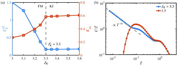
Figure S13: (a) shows the ground-state spin structure at $k=0$ and Kondo correlation function $K_{nn}$, as function of Kondo coupling $J_{K}$, with $J_{H}=-1$, $t=2$, $N=36\times 2$. (b) shows $C/T$ data with $N=36\times 2$ and $J_{K}=3.3,~{}3.5$. At the quantum critical point, the lower part of $C/T$ diverges algebraically with $\alpha\sim 0.7$.

We further perform XTRG simulation at the putative phase transition point $J_{K}^{c}=3.3$. As shown in Fig. S13 (b), the low temperature heat capacity displays algebraic behavior as $C/T\sim T^{-0.7}$, signalling quantum criticality.

IV.2 Determination of the crossover temperature

Although there is no finite-temperature phase transition in 1D quantum system, the crossover temperature can be determined form the thermodynamic quantities and correlation function. In the FM phase, we obtain the crossover temperature $T^{*}_{\rm C}$ from the the temperature derivatives of local moment correlations -$dF_{nn}/dT$ with $F_{nn}=\frac{1}{L-1}\sum_{n}\langle{\bf S}_{n}\cdot{\bf S}_{n+1}\rangle$. The corresponding result is shown in Fig. S14(a). As the Kondo coupling increasing, the crossover temperature decreases. In the Kondo insulator phase, we determine the crossover temperature by -$dK_{nn}/dT$. As shown in Fig. S14(b), $T_{\rm K}$ has positive correlation to the Kondo coupling $J_{K}$. All the above calculation are performed by XTRG with $N=36\times 2$ and $D=1600$ and the corresponding result is shown in Fig. 1(a) of the main text.

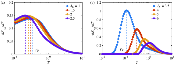
Figure S14: (a) shows the -$dF_{nn}/dT$ in the FM phase and (b) shows the -$dK_{nn}/dT$ in the KI phase with $N=36\times 2$ and $D=1600$. The dashed line indicates $T_{\rm C}^{*}$ and $T_{\rm K}$ respectively.

IV.3 Finite-temperature properties in the FM phase

Here we discuss the Kondo correlation $K_{nn}$ and FM spin structure factor $S^{zz}_{\Gamma}$ in the FM region (with the same model parameter in Fig. 3 of the main text). As shown in Fig. S15, $K_{nn}$ also displays a minimum value around $T_{\rm d}^{*}$, while $S^{zz}_{\Gamma}$ behaves similarly for both $J_{K}=0$ and $J_{K}\neq 0$ above $T_{\rm d}^{*}$. These results indicate that the Kondo coupling $J_{K}$ prominently changes the thermodynamical properties below $T_{\rm d}^{*}$. Notably, $S^{zz}_{\Gamma}$ keeps increasing as system cooling down even below $T_{\rm d}^{*}$ which means that the local moments are not fully screened by the itinerant electrons in this case.

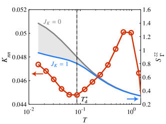
Figure S15: Kondo correlation $K_{nn}$ (red circle) and spin structure factor $S^{zz}_{\Gamma}$ (blue solid line) with $N=16\times 2$, $t=2$, $J_{H}=-1$, $J_{K}=1$ and $D=1600$. The gray solid line shows $S^{zz}_{\Gamma}$ with $J_{K}=0$ and the gray shadow region shows the difference between $J_{K}=0$ and $J_{K}=1$. The vertical point-solid line shows the minimum damping temperature $T_{\rm d}^{*}$ determine by $\gamma_{\pi}$ (see Fig. 3 in the main text).

IV.4 Determination of the mean-field phase diagram

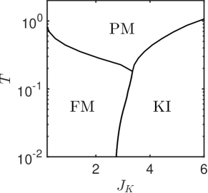
Figure S16: Phase diagram of the 1D FMKH model ($t=2$, $J_{H}=-1$), based on the effective mean field theory by solving Eq. (S59) self-consistently. The FM phase is identified with nonzero $m_{c}$ and $m_{f}$. The KI phase is identified with nonzero $V$.

In this section, we discuss an effective mean-field theory which can treat the FM order and local Kondo screening effect on an equal footing. Hence a complete phase diagram containing both the FM phase at small $J_{K}$ and KI phase at large $J_{K}$ can be obtained. The starting point of this effective mean-field theory is to notice that the Kondo coupling term can be decomposed into longitudinal and transversal parts [47],

$$\boldsymbol{S}_{n}\cdot\boldsymbol{s}_{n}=S_{n}^{z}s_{n}^{z}-\frac{1}{4}[(c^{\dagger}_{n\uparrow}f_{n\uparrow}+f^{\dagger}_{n\downarrow}c_{n\downarrow})^{2}+(c^{\dagger}_{n\downarrow}f_{n\downarrow}+f^{\dagger}_{n\uparrow}c_{n\uparrow})^{2}],$$ (S42)

where we have used the pseudo-fermion representation for the local spin $S_{n}=\frac{1}{2}\sum_{\alpha\beta}f^{\dagger}_{n\alpha}\boldsymbol{\sigma}_{\alpha\beta}f_{n\beta}$, with a local constraint

$$\sum_{\sigma}f^{\dagger}_{n\sigma}f_{n\sigma}=1,$$ (S43)

enforced at each site $n$. Equation (S42) inspired one to define, besides the standard FM order parameters

$$m_{c}=\expectationvalue{S^{z}_{n}},\quad m_{f}=\expectationvalue{s^{z}_{n}},$$ (S44)

also the Kondo hybridization order parameter as follows,

$$V=\expectationvalue{c^{\dagger}_{n\uparrow}f_{n\uparrow}+f^{\dagger}_{n\downarrow}c_{n\downarrow}}.$$ (S45)

Using these order parameters, one can decouple the original Hamiltonian, $H=H_{t}+H_{H}+H_{K}$ with

$$H_{t} = -t\sum_{n}c^{\dagger}_{n}c_{n+1}+\text{H.c.},$$ (S46)

$$H_{H} = J_{H}\sum_{n}\boldsymbol{S}_{n}\cdot\boldsymbol{S}_{n+1},$$ (S47)

$$H_{K} = J_{K}\sum_{n}\boldsymbol{S}_{n}\cdot\boldsymbol{s}_{n},$$ (S48)

to a quadratic form. Firstly, the hopping term, $H_{t}$, is unchanged. Secondly, the ferromagnetic Heisenberg term becomes

$$H_{H}\rightarrow J_{H}\sum_{n}m_{f}(f^{\dagger}_{n\uparrow}f_{n\uparrow}-f^{\dagger}_{n\downarrow}f_{n\downarrow})-J_{H}Lm_{f}^{2}.$$ (S49)

And lastly, the Kondo coupling term becomes

$$H_{K} \rightarrow J_{K}\sum_{n=1}^{L}\left[\frac{m_{c}}{2}(f_{n\uparrow}^{{\dagger}}f_{n\uparrow}-f^{{\dagger}}_{n\downarrow}f_{n\downarrow})+\frac{m_{f}}{2}(c^{{\dagger}}_{n\uparrow}c_{n\uparrow}-c^{{\dagger}}_{n\downarrow}c_{n\downarrow})-m_{c}m_{f}\right]$$ (S50)

$$+J_{K}\sum_{n=1}^{L}\left[-\frac{1}{2}V(c^{{\dagger}}_{n\uparrow}f_{n\uparrow}+f^{{\dagger}}_{n\downarrow}c_{n\downarrow})-\frac{1}{2}V(c^{{\dagger}}_{n\downarrow}f_{n\downarrow}+f^{{\dagger}}_{n\uparrow}c_{i\uparrow})+\frac{1}{2}V^{2}\right].$$

We also introduce a Lagrangian multiplier $\lambda$ to enforce the local constraint Eq. (S43),

$$\lambda\sum_{n=1}^{L}(f^{{\dagger}}_{n\sigma}f_{n\sigma}-1),$$ (S51)

and a chemical potential $\mu$ to fix the total $c$ fermion number at half filling,

$$-\mu\sum_{n=1}^{L}(c^{{\dagger}}_{n}c_{n}-1).$$ (S52)

Hence the mean-field Hamiltonian in momentum space can be written in a compact form

$$H_{\text{MF}}=\sum_{k,\sigma}(c^{{\dagger}}_{k\sigma},f^{{\dagger}}_{k\sigma})\left(\begin{array}[]{cc}\varepsilon_{k\sigma}&-\frac{1}{2}J_{K}V\\ -\frac{1}{2}J_{K}V&\lambda_{\sigma}\end{array}\right)\left(\begin{array}[]{c}c_{k\sigma}\\ f_{k\sigma}\end{array}\right)+L\varepsilon_{0},$$ (S53)

where

$$\varepsilon_{k\sigma} = -2t\cos k+\frac{J_{K}m_{f}}{2}\sigma-\mu,$$ (S54)

$$\lambda_{\sigma} = \lambda+\left(\frac{J_{K}m_{c}}{2}+J_{H}m_{f}\right)\sigma,$$ (S55)

$$\varepsilon_{0} = \frac{J_{K}V^{2}}{2}-J_{K}m_{c}m_{f}-\lambda+\mu-J_{H}m_{f}^{2}.$$ (S56)

The quasiparticle excitation spectra are thus obtained by

$$E_{k\sigma l} = \frac{1}{2}\left[\varepsilon_{k\sigma}+\lambda_{\sigma}+l\sqrt{(\varepsilon_{k\sigma}-\lambda_{\sigma})^{2}+(J_{K}V)^{2}}\right],$$ (S57)

which corresponds to four quasiparticle bands, with $\sigma=\pm$ and $l=\pm$. The corresponding Helmholtz free energy density reads

$$f=-\frac{1}{\beta L}\sum_{k}\sum_{l,\sigma=\pm}\log[1+\exp(-\beta E_{k\sigma l})]+\varepsilon_{0}.$$ (S58)

which should be minimized with respect to the five unknown parameters:

$$0 =\partial_{m_{f}}f$$

$$=\frac{1}{L}\sum_{k}\sum_{l,\sigma=\pm}\frac{e^{-\beta E_{k\sigma l}}}{1+\exp(-\beta E_{k\sigma l})}\partial_{m_{f}}E_{k\sigma l}-J_{K}m_{c}-2J_{H}m_{f}$$

$$=\frac{1}{L}\sum_{k}\sum_{l,\sigma=\pm}n(E_{k\sigma l})\sigma\left[\frac{J_{H}}{2}+\frac{J_{K}}{4}+l\left(\frac{J_{K}}{4}-\frac{J_{H}}{2}\right)\frac{\varepsilon_{k\sigma}-\lambda_{\sigma}}{\sqrt{(\varepsilon_{k\sigma}-\lambda_{\sigma})^{2}+(KV)^{2}}}\right]-J_{K}m_{c}-2J_{H}m_{f}$$ (S59a)

$$0 =\partial_{m_{c}}f$$

$$=\frac{1}{L}\sum_{k}\sum_{l,\sigma=\pm}n(E_{k\sigma l})\frac{J_{K}\sigma}{4}\left[1-l\frac{\varepsilon_{k\sigma}-\lambda_{\sigma}}{\sqrt{(\varepsilon_{k\sigma}-\lambda_{\sigma})^{2}+(J_{K}V)^{2}}}\right]-J_{K}m_{f}$$ (S59b)

$$0 =\partial_{V}f$$

$$=\frac{1}{L}\sum_{k}\sum_{l,\sigma=\pm}n(E_{k\sigma l})\frac{lJ_{K}^{2}V/2}{\sqrt{(\varepsilon_{k\sigma}-\lambda_{\sigma})^{2}+(J_{K}V)^{2}}}+J_{K}V$$ (S59c)

$$0 =\partial_{\lambda}f$$

$$=\frac{1}{L}\sum_{k}\sum_{l,\sigma=\pm}n(E_{k\sigma l})\frac{1}{2}\left[1-l\frac{\varepsilon_{k\sigma}-\lambda_{\sigma}}{\sqrt{(\varepsilon_{k\sigma}-\lambda_{\sigma})^{2}+(J_{K}V)^{2}}}\right]-1$$ (S59d)

$$0 =\partial_{\mu}f$$

$$=\frac{1}{L}\sum_{k}\sum_{l,\sigma=\pm}n(E_{k\sigma l})\frac{1}{2}\left[-1-l\frac{\varepsilon_{k\sigma}-\lambda_{\sigma}}{\sqrt{(\varepsilon_{k\sigma}-\lambda_{\sigma})^{2}+(J_{K}V)^{2}}}\right]+1,$$ (S59e)

with $n(E_{k\sigma l})=(e^{\beta E_{k\sigma l}}+1)^{-1}$ being the Fermi function. We numerically solve above five equations self-consistently. The resulting finite temperature phase diagram for $(J_{H},t)=(-1,2)$ is shown in Fig. S16.

V Excitation Spectrum in the Strong-coupling Limit: Bond-operator Theory

In this appendix, we give a strong-coupling mean-field analysis of the FMKH model for $K\gg J,t$, using bond-operator theory. This approach was originally proposed by Sachdev and Bhatt for the dimerized spin systems [50]. Its generalization to the Kondo lattice systems was firstly given by Jurecka and Brenig [51]. R. Eder recently gave an improved treatment to obtained both the fermionic quasiparticle and spin excitation spectrum for the Kondo lattice [52]. We here generalize it to the FMKH model.

V.1 Bond-operator basis

The Kondo-coupling term leads to eight eigenstates, defined as follows [51]:

$$\ket{s} =s^{\dagger}\ket{0}=\frac{1}{\sqrt{2}}(f^{\dagger}_{\downarrow}c^{\dagger}_{\uparrow}+c^{\dagger}_{\downarrow}f^{\dagger}_{\uparrow})\ket{0},$$ (S60a)

$$\ket{t_{x}} =t^{\dagger}_{x}\ket{0}=\frac{-1}{\sqrt{2}}(c^{\dagger}_{\uparrow}f^{\dagger}_{\uparrow}-c^{\dagger}_{\downarrow}f^{\dagger}_{\downarrow})\ket{0},$$ (S60b)

$$\ket{t_{y}} =t^{\dagger}_{y}\ket{0}=\frac{\rm i}{\sqrt{2}}(c^{\dagger}_{\uparrow}f^{\dagger}_{\uparrow}+c^{\dagger}_{\downarrow}f^{\dagger}_{\downarrow})\ket{0},$$ (S60c)

$$\ket{t_{z}} =t^{\dagger}_{z}\ket{0}=\frac{1}{\sqrt{2}}(c^{\dagger}_{\uparrow}f^{\dagger}_{\downarrow}+c^{\dagger}_{\downarrow}f^{\dagger}_{\uparrow})\ket{0},$$ (S60d)

$$\ket{a_{\sigma}} =a^{\dagger}_{\sigma}\ket{0}=f^{\dagger}_{\sigma}\ket{0},$$ (S60e)

$$\ket{b_{\sigma}} =b^{\dagger}_{\sigma}\ket{0}=c^{\dagger}_{\uparrow}c^{\dagger}_{\downarrow}f^{\dagger}_{\sigma}\ket{0}.$$ (S60f)

Note the $f$ fermion has to satisfy the local constraint at each site,

$$f^{\dagger}_{n\sigma}f_{n\sigma}=1,\quad\forall\ n.$$ (S61)

Hereafter Einstein summation rule over repeated Greek alphabet (i.e., spin indices) is assumed. When the spin index is omitted, the corresponding operators should be viewed as a two-component object. The first four particles in Eq. (S60) are bosons; and the rest are fermions. They together satisfy the local constraint

$$s^{\dagger}_{n}s_{n}+a^{\dagger}_{n\sigma}a_{n\sigma}+b^{\dagger}_{n\sigma}b_{n\sigma}+\boldsymbol{t}^{\dagger}_{n}\cdot\boldsymbol{t}_{n}=1,\quad\forall n$$ (S62)

which ensures Eq. (S61) automatically.

V.2 Operators in bond-operator representation

Here we give explicit form of relevant operators in this representation. First of all, the spin operator for itinerant electrons and local moments becomes, respectively,

$$s^{\sigma}_{n} =\frac{1}{2}(-t^{\dagger}_{n\sigma}s_{n}-s^{\dagger}_{n}t_{n\sigma}-{\rm i}\epsilon_{\sigma\alpha\beta}t^{\dagger}_{n\alpha}t_{n\beta}),$$ (S63)

$$S^{\sigma}_{n} =\frac{1}{2}(t^{\dagger}_{n\sigma}s_{n}+s^{\dagger}_{n}t_{n\sigma}-{\rm i}\epsilon_{\sigma\alpha\beta}t^{\dagger}_{n\alpha}t_{n\beta})+S^{\sigma}_{a,n}+S^{\sigma}_{b,n},$$ (S64)

where $S_{a,n}^{\mu}=\frac{1}{2}a^{\dagger}_{n}\sigma^{\mu}a_{n}$ and $S_{b,n}^{\mu}=\frac{1}{2}b^{\dagger}_{n}\sigma^{\mu}b_{n}$. Then the Kondo coupling term can be shown to be

$$J_{K}\sum_{n}{\bf S}_{n}\cdot{\boldsymbol{s}}_{n}=\sum_{n}[\frac{3J_{K}}{4}(b^{\dagger}_{n\sigma}b_{n\sigma}+a^{\dagger}_{n\sigma}a_{n\sigma})+J_{K}\boldsymbol{t}^{\dagger}_{n}\cdot\boldsymbol{t}_{n}]-\frac{3J_{N}K}{4},$$ (S65)

which is diagonal as expected. Next, the itinerant electron annihilation operator becomes

$$c_{n}=\frac{1}{\sqrt{2}}[(-s_{n}+\boldsymbol{t}_{n}\cdot\boldsymbol{\tau}){\rm i}\tau^{y}a^{\dagger}_{n}+(s^{\dagger}_{n}+\boldsymbol{t}^{\dagger}_{n}\cdot\boldsymbol{\tau})b_{n}],$$ (S66)

from which we can obtain the hopping term for itinerant electrons,

$$-t\sum_{n}c^{\dagger}_{n}c_{n+1}+\text{H.c.}=H_{c1}+H_{c2}+H_{c3}+H_{c4},$$ (S67)

with

$$H_{c1} =\frac{1}{2}\sum_{n,m}t_{n,m}[(-s^{\dagger}_{n}s_{m}a^{\dagger}_{m}a_{n}+s_{n}s^{\dagger}_{m}b^{\dagger}_{n}b_{m}-(s_{n}s_{m}b^{\dagger}_{n}{\rm i}\tau^{y}a^{\dagger}_{m}+\text{H.c.})],$$ (S68)

$$H_{c2} =\frac{1}{2}\sum_{n,m}t_{n,m}[-\boldsymbol{t}^{\dagger}_{n}\cdot\boldsymbol{t}_{m}a^{\dagger}_{m}a_{n}+\boldsymbol{t}_{n}\cdot\boldsymbol{t}^{\dagger}_{m}b^{\dagger}_{n}b_{m}+(\boldsymbol{t}_{n}\cdot\boldsymbol{t}_{m}b^{\dagger}_{n}{\rm i}\tau^{y}a^{\dagger}_{m}+\text{H.c.})],$$ (S69)

$$H_{c3} =\frac{1}{2}\sum_{n,m}t_{n,m}\{(s^{\dagger}_{n}\boldsymbol{t}_{m}+s_{m}\boldsymbol{t}^{\dagger}_{n})\cdot(\boldsymbol{a}_{m,n}+\boldsymbol{b}_{m,n})+[(s_{m}\boldsymbol{t}_{n}-s_{n}\boldsymbol{t}_{m})\cdot\boldsymbol{\pi}^{\dagger}_{n,m}+\text{H.c.}]\},$$ (S70)

$$H_{c4} =\frac{1}{2}\sum_{n,m}t_{n,m}[-\boldsymbol{t}^{\dagger}_{n}\times\boldsymbol{t}_{m}\cdot{\rm i}(\boldsymbol{a}_{m,n}+\boldsymbol{b}_{m,n})+(\boldsymbol{t}_{m}\times\boldsymbol{t}_{n}\cdot{\rm i}\boldsymbol{\pi}^{\dagger}_{m,n}+\text{H.c.})],$$ (S71)

Here $t_{m,n}=-t$ for the nearest-neighbors, and vanishing otherwise. And the following vectorized operators have been used: $\boldsymbol{a}_{m,n}=a^{\dagger}_{m}\boldsymbol{\tau}b_{n}$, $\boldsymbol{b}_{m,n}=b^{\dagger}_{m}\boldsymbol{\tau}b_{n}$ and $\boldsymbol{\pi}_{m,n}^{\dagger}=b^{\dagger}_{m}\boldsymbol{\tau}{\rm i}\tau^{y}a^{\dagger}_{n}$. Interestingly, the hopping term, which is originally quadratic, now becomes quartic. Such behavior is common for strong-coupling approaches, see also [63]. Lastly, the Heisenberg coupling term for localized spins becomes

$$J_{H}\sum_{n}{\bf S}_{n}\cdot{\bf S}_{n+1}=H_{s1}+H_{s2}+H_{s3}+H_{s4},\quad J>0,$$ (S72)

where

$$\begin{split}H_{s1}&=\frac{1}{8}\sum_{n,m}J_{n,m}(\boldsymbol{t}^{\dagger}_{n}s_{n}+s^{\dagger}_{n}\boldsymbol{t}_{n})\cdot(\boldsymbol{t}^{\dagger}_{m}s_{m}+s^{\dagger}_{m}\boldsymbol{t}_{m}),\\ H_{s2}&=-\frac{\rm i}{4}\sum_{n,m}J_{n,m}(\boldsymbol{t}^{\dagger}_{n}s_{n}+s^{\dagger}_{n}\boldsymbol{t}_{n})\cdot\boldsymbol{t}^{\dagger}_{m}\times\boldsymbol{t}_{m},\\ H_{s3}&=-\frac{1}{8}\sum_{n,m}J_{n,m}[(\boldsymbol{t}^{\dagger}_{n}\cdot\boldsymbol{t}^{\dagger}_{m})(\boldsymbol{t}_{n}\cdot\boldsymbol{t}_{m})-t^{\dagger}_{n\alpha}t_{n\beta}t^{\dagger}_{m\beta}t_{m\alpha}],\\ H_{s4}&=\frac{1}{2}\sum_{n,m}J_{n,m}[(\boldsymbol{t}^{\dagger}_{n}s_{n}+s^{\dagger}_{n}\boldsymbol{t}_{n}-i\boldsymbol{t}^{\dagger}_{n}\times\boldsymbol{t}_{n})\cdot(\boldsymbol{S}_{a,m}+\boldsymbol{S}_{b,m})+(\boldsymbol{S}_{a,n}+\boldsymbol{S}_{b,n})\cdot(\boldsymbol{S}_{a,m}+\boldsymbol{S}_{b,m})],\end{split}$$ (S73)

with $J_{n,m}=J_{H}<0$ for nearest neighbors and vanishing otherwise.

V.3 Simplest mean-field approximation

In the simplest mean-field approach, we condense singlets, $s^{\dagger}_{n},s_{n}\rightarrow s$, and collect terms up to quadratic order in the remaining operators. The Kondo coupling term is unchanged,

$$J_{K}\sum_{n}\boldsymbol{S}_{n}\cdot\boldsymbol{s}_{n} \rightarrow\sum_{n}[\frac{3J_{K}}{4}(b^{\dagger}_{n\sigma}b_{n\sigma}+a^{\dagger}_{n\sigma}a_{n\sigma})+J_{K}\boldsymbol{t}^{\dagger}_{n}\cdot\boldsymbol{t}_{n}]-\frac{3NJ_{K}}{4}$$

$$=\sum_{k}[\frac{3J_{K}}{4}(b^{\dagger}_{k}b_{k}+a^{\dagger}_{k}a_{k})+J_{K}\boldsymbol{t}^{\dagger}_{k}\cdot\boldsymbol{t}_{k}]-\frac{3NJ_{K}}{4}.$$ (S74)

The hopping term for itinerant electrons becomes

$$-t\sum_{n}c^{\dagger}_{n}c_{n+1}+\text{H.c.} \rightarrow\frac{s^{2}}{2}\sum_{n,m}t_{n,m}[(-a^{\dagger}_{m}a_{n}+b^{\dagger}_{n}b_{m}-(b^{\dagger}_{n}{\rm i}\tau^{y}a^{\dagger}_{m}+\text{H.c.})]$$

$$=-ts^{2}\sum_{k}[\cos k(-a^{\dagger}_{k}a_{k}+b^{\dagger}_{k}b_{k})-(\cos kb^{\dagger}_{k}{\rm i}\tau^{y}a^{\dagger}_{-k}+\text{H.c.})].$$ (S75)

And finally the Heisenberg coupling term becomes

$$J_{H}\sum_{n}\boldsymbol{S}_{n}\cdot\boldsymbol{S}_{n+1} \rightarrow\frac{s^{2}}{8}\sum_{n,m}J_{n,m}(\boldsymbol{t}^{\dagger}_{n}+\boldsymbol{t}_{n})\cdot(\boldsymbol{t}^{\dagger}_{m}+\boldsymbol{t}_{m})$$

$$=\frac{s^{2}J_{H}}{4}\sum_{k}[2\cos k\boldsymbol{t}^{\dagger}_{k}\cdot\boldsymbol{t}_{k}+(\cos k\boldsymbol{t}^{\dagger}_{k}\cdot\boldsymbol{t}^{\dagger}_{-k}+\text{H.c.})].$$ (S76)

We further introduce two Lagrange multipliers, $\lambda$ and $\mu$, to enforce Eq. (S62) globally,

$$-\lambda\sum_{n}\left[s^{\dagger}_{n}s_{n}+\boldsymbol{t}^{\dagger}_{n}\cdot\boldsymbol{t}_{n}+a^{\dagger}_{n}a_{n}+b^{\dagger}_{n}b_{n}-1\right]$$ (S77)

and also to fix the $c$ fermion number at half-filling,

$$0 =-\mu\sum_{n}\left(s^{\dagger}_{n}s_{n}+\boldsymbol{t}^{\dagger}_{n}\cdot\boldsymbol{t}_{n}+2b^{\dagger}_{n}b_{n}-1\right)$$

$$=-\mu\sum_{n}\left(b^{\dagger}_{n}b_{n}-a^{\dagger}_{n}a_{n}\right).$$ (S78)

Thus the resulting mean-field Hamiltonian reads

$$H_{{\text{MF}}}=H_{F}+H_{B}-\frac{3NJ_{K}}{4}+N(1-s^{2})\lambda,$$ (S79)

where

$$H_{F} =\sum_{k}[(\frac{3J_{K}}{4}-\lambda+\mu+s^{2}t\cos k)a^{\dagger}_{k}a_{k}+(\frac{3J_{K}}{4}-\lambda-\mu-s^{2}t\cos k)b^{\dagger}_{k}b_{k}+(s^{2}t\cos kb^{\dagger}_{k}{\rm i}\tau^{y}a^{\dagger}_{-k}+\text{H.c.})],$$ (S80)

$$H_{B} =\sum_{k}[(J_{K}-\lambda-\frac{s^{2}J}{2}\cos k)\boldsymbol{t}^{\dagger}_{k}\cdot\boldsymbol{t}_{k}+(\frac{s^{2}J_{H}}{4}\cos k\boldsymbol{t}^{\dagger}_{k}\cdot\boldsymbol{t}^{\dagger}_{-k}+\text{H.c.})].$$ (S81)

V.4 Solving the fermionic part

The fermionic sector, Eq. (S80), can be written as

$$H_{F}=\sum_{k}\begin{pmatrix}a^{\dagger}_{k}&b^{\dagger}_{k}\end{pmatrix}A_{k}\begin{pmatrix}a_{k}\\ b_{k}\end{pmatrix}+\left[\frac{1}{2}\begin{pmatrix}a^{\dagger}_{k}&b^{\dagger}_{k}\end{pmatrix}B_{k}\begin{pmatrix}a^{\dagger}_{-k}\\ b^{\dagger}_{-k}\end{pmatrix}+\text{H.c.}\right],$$ (S82)

where

$$A_{k} =\begin{pmatrix}\frac{3J_{K}}{4}-\lambda+\mu+s^{2}t\cos k&0\\ 0&\frac{3J_{K}}{4}-\lambda-\mu-s^{2}t\cos k\end{pmatrix},$$ (S83)

$$B_{k} =\begin{pmatrix}0&s^{2}t\cos k{\rm i}\tau^{y}\\ s^{2}t\cos k{\rm i}\tau^{y}&0\end{pmatrix}.$$ (S84)

By defining the Nambu spinor $\psi^{\dagger}_{k}=\begin{pmatrix}a^{\dagger}_{k}&b^{\dagger}_{k}&a_{-k}&b_{-k}\end{pmatrix}$, Eq. (S82) can be further recast into the Bogoliubov-de Gennes (BdG) form, $H_{F}=\frac{1}{2}\sum_{k}\psi^{\dagger}_{k}M_{k}\psi_{k}+\frac{1}{2}\sum_{k}\Tr{A_{k}}$, where the BdG matrix reads $M_{k}=\begin{pmatrix}A_{k}&B_{k}\\ B^{\dagger}_{k}&-A^{T}_{-k}\end{pmatrix}$. This matrix can be diagonalized by using a unitary matrix $U_{k}$, such that $\psi_{k}=U_{k}\varphi_{k}$, and

$$\frac{1}{2}\sum_{k}\psi^{\dagger}_{k}M_{k}\psi_{k} =\frac{1}{2}\sum_{k}\varphi^{\dagger}_{k}D_{k}\varphi_{k}$$

$$=\sum_{k}e_{a,k}\tilde{a}^{\dagger}_{k}\tilde{a}_{k}+e_{b,k}\tilde{b}_{k}\tilde{b}_{k}-\sum_{k}\sum_{l=a,b}e_{l,k}.$$ (S85)

Note that there is a factor of two for the last term, which is due to double degeneracy. Here $\varphi^{\dagger}_{k}=\begin{pmatrix}\tilde{a}^{\dagger}_{k}&\tilde{b}^{\dagger}_{k}&\tilde{a}_{k}&\tilde{b}_{k}\end{pmatrix}$ is the Nambu spinor form of the fermionic quasiparticle, $D_{k}$ is a diagonal matrix, and the eigenvalues are

$$e_{a(b),k}=\sqrt{(\frac{3J_{K}}{4}-\lambda)^{2}+s^{4}t^{2}\cos^{2}k}\pm\mu\pm s^{2}t\cos k.$$ (S86)

Hence Eq. (S80) becomes

$$H_{F}=\sum_{k}e_{a,k}\tilde{a}_{k}^{\dagger}\tilde{a}_{k}+e_{b,k}\tilde{b}^{\dagger}_{k}\tilde{b}_{k}-\sum_{k}\sum_{l=a,b}e_{l,k}+\frac{1}{2}\sum_{k}\Tr{A_{k}}.$$ (S87)

V.5 Solving the bosonic part

The bosonic sector, Eq. (S81) can be further written as

$$H_{B}=\sum_{k}\boldsymbol{t}^{\dagger}_{k}A_{k}\boldsymbol{t}_{k}+\left(\frac{1}{2}\boldsymbol{t}^{\dagger}_{k}B_{k}\boldsymbol{t}^{\dagger}_{-k}+\text{H.c.}\right),$$ (S88)

where

$$A_{k}=K-\lambda+\frac{s^{2}J_{H}}{2}\cos k,$$ (S89)

and $B_{k}=\frac{s^{2}J_{H}}{2}\cos k$. By defining the Nambu spinor $\psi^{\dagger}_{k}=\begin{pmatrix}\boldsymbol{t}^{\dagger}_{k}&\boldsymbol{t}_{-k}\end{pmatrix}$, Eq. (S88) can be written in the BdG form, $H_{b}=\frac{1}{2}\sum_{k}\psi^{\dagger}_{k}M_{k}\psi_{k}-\sum_{k}\frac{3}{2}\Tr{A_{k}}$. Note that there is a factor of $3$ for the last term, which is due to triple degeneracy. And the BdG matrix reads $M_{k}=\begin{pmatrix}A_{k}&B_{k}\\ B^{\dagger}_{k}&A^{T}_{-k}\end{pmatrix}$. This matrix is diagonalized by a pseudounitary matrix $U_{k}=\begin{pmatrix}\cosh\theta_{k}&\sinh\theta_{k}\\ \sinh\theta_{k}&\cosh\theta_{k}\end{pmatrix}$, with $\tanh 2\theta_{k}=-\frac{s^{2}J_{H}}{2}\cos k/(J_{K}-\lambda+\frac{s^{2}J_{H}}{2}\cos k)$, such that $\psi_{k}=U_{k}\varphi_{k}$, and

$$\frac{1}{2}\sum_{k}\psi^{\dagger}_{k}M_{k}\psi_{k}=\frac{1}{2}\sum_{k}\varphi^{\dagger}_{k}\begin{pmatrix}\omega_{k}&\\ &\omega_{k}\end{pmatrix}\varphi_{k}=\sum_{k}\omega_{k}\tilde{\boldsymbol{t}}_{k}\tilde{\boldsymbol{t}}_{k}+\frac{3}{2}\sum_{k}\omega_{k}.$$ (S90)

Note again the factor of 3 in the last term. Here $\varphi^{\dagger}_{k}=\begin{pmatrix}\tilde{\boldsymbol{t}}^{\dagger}_{k}&\tilde{\boldsymbol{t}}_{-k}\end{pmatrix}$ is the Nanbu spinor form of the triplon, with dispersion

$$\omega_{k}=\sqrt{(J_{K}-\lambda)^{2}+(J_{K}-\lambda)s^{2}J_{H}\cos k},$$ (S91)

Hence Eq. (S81) becomes

$$H_{b}=\sum_{k}\omega_{k}\tilde{\boldsymbol{t}}^{\dagger}_{k}\tilde{\boldsymbol{t}}_{k}+\frac{3}{2}\sum_{k}\omega_{k}-\frac{3}{2}\sum_{k}\Tr{A_{k}}.$$ (S92)

V.6 Helmholtz free energy and its minimization

Based on above analysis, we can now obtain the Helmholtz free energy density of the system,

$$f =-\frac{2}{\beta N}\sum_{k}\sum_{l=a,b}\log[1+\exp(-\beta e_{l,k})]+\frac{3}{\beta N}\log[1-\exp(-\beta\omega_{k})]$$

$$\quad-\frac{1}{N}\sum_{k}\sum_{l=a,b}e_{l,k}+\frac{1}{2N}\sum_{k}\Tr{A_{F,k}})+\frac{3}{2N}\sum_{k}\omega_{k}-\frac{3}{2N}\sum_{k}\Tr{A_{B,k}}$$ (S93)

$$\quad-\frac{3J_{K}}{4}+\lambda(1-s^{2}),$$ (S94)

where $A_{B,k}$ and $A_{F,k}$ are given by Eq. (S89) and (S83), respectively.

There are three unknown parameters: $s$, $\lambda$ and $\mu$, which have to be determined by minimizing the free energy density. For $\lambda$, we have

$$0 =\partial_{\lambda}F$$ (S95)

$$=\frac{3}{N}\sum_{k}\left[f_{B}(\omega_{k})+\frac{1}{2}\right]\frac{-J_{K}+\lambda-\frac{s^{2}J_{H}}{2}\cos k}{\sqrt{(J_{K}-\lambda)^{2}+(J_{K}-\lambda)s^{2}J_{H}\cos k}}$$

$$\quad-\frac{2}{N}\sum_{k}\sum_{l=a,b}\left[f_{F}(e_{l,k})-\frac{1}{2}\right]\frac{\frac{3J_{K}}{4}-\lambda}{\sqrt{(\frac{3J_{K}}{4}-\lambda)^{2}+s^{4}t^{2}\cos^{2}k}}$$

$$\quad+\frac{1}{2}-s^{2}.$$ (S96)

For $\mu$, we have

$$0=\partial_{\mu}f=\frac{2}{N}\sum_{k}[f_{F}(e_{a,k})-f_{F}(e_{b,k})].$$ (S97)

And for $s$, we have

$$0 =\partial_{s}F$$ (S98)

$$=-\frac{3}{N}\sum_{k}\left[f_{B}(\omega_{k})+\frac{1}{2}\right]\frac{-(J_{K}-\lambda)sJ_{H}\cos k}{\sqrt{(J_{K}-\lambda)^{2}+(J_{K}-\lambda)s^{2}J_{H}\cos k}}$$

$$\quad+\frac{2}{N}\sum_{k}\left[f_{F}(e_{a,k})-\frac{1}{2}\right]\left[\frac{2s^{3}t^{2}\cos^{2}k}{\sqrt{(\frac{3J_{K}}{4}-\lambda)^{2}+s^{4}t^{2}\cos^{2}k}}+2st\cos k\right]$$

$$\quad+\frac{2}{N}\sum_{k}\left[f_{F}(e_{a,k})-\frac{1}{2}\right]\left[\frac{2s^{3}t^{2}\cos^{2}k}{\sqrt{(\frac{3J_{K}}{4}-\lambda)^{2}+s^{4}t^{2}\cos^{2}k}}-2st\cos k\right]$$

$$\quad-2\lambda s.$$ (S99)

Here $f_{F(B)}(x)=(e^{\beta x}\pm 1)^{-1}$ is the Fermi (Bose) function.

We numerically solve these three coupled nonlinear equations, (S96), (S97) and (S99). The finite-temperature crossover from paramagnetic (PM) phase to the Kondo insulating (KI) phase can be characterized by the onset of a nonzero $s$. In Fig. S17, we plot the condensed singlet $\langle s\rangle$ as a function of temperature $T$ and the Kondo coupling $J_{K}$. It is found that this strong coupling approach is in excellent agreement with the XTRG result for large $J_{K}$.

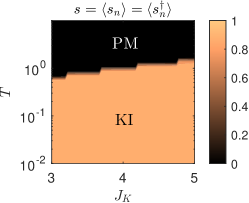
Figure S17: Finite-temperature phase diagram for large $J_{K}$, obtained by bond-operator theory, with other parameters chosen the same as Fig. 1(a).

References

Verchenko et al. [2015]V. Y. Verchenko, A. A. Tsirlin, A. V. Sobolev, I. A. Presniakov, and A. V. Shevelkov, Ferromagnetic order,
strong magnetocrystalline anisotropy, and magnetocaloric effect in the
layered telluride Fe3-δGeTe2, Inorganic Chemistry 54, 8598 (2015).
Deng et al. [2018]Y. Deng, Y. Yu, Y. Song, J. Zhang, N. Z. Wang, Z. Sun, Y. Yi, Y. Z. Wu, S. Wu, J. Zhu, J. Wang, X. H. Chen, and Y. Zhang, Gate-tunable room-temperature ferromagnetism in two-dimensional
Fe3GeTe2, Nature 563, 94 (2018).
Kim et al. [2018]K. Kim, J. Seo, E. Lee, K. T. Ko, B. S. Kim, B. G. Jang, J. M. Ok, J. Lee, Y. J. Jo, W. Kang, J. H. Shim, C. Kim, H. W. Yeom, B. Il Min, B.-J. Yang, and J. S. Kim, Large anomalous hall current induced
by topological nodal lines in a ferromagnetic van der Waals semimetal, Nature Materials 17, 794 (2018).
Fei et al. [2018]Z. Fei, B. Huang, P. Malinowski, W. Wang, T. Song, J. Sanchez, W. Yao,
D. Xiao, X. Zhu, A. F. May, W. Wu, D. H. Cobden, J.-H. Chu, and X. Xu, Two-dimensional itinerant
ferromagnetism in atomically thin Fe3GeTe2, Nature Materials 17, 778 (2018).
Wang et al. [2019a]X. Wang, J. Tang, X. Xia, C. He, J. Zhang, Y. Liu, C. Wan, C. Fang, C. Guo, W. Yang, Y. Guang, X. Zhang, H. Xu, J. Wei, M. Liao, X. Lu, J. Feng, X. Li, Y. Peng, H. Wei, R. Yang, D. Shi, X. Zhang, Z. Han, Z. Zhang, G. Zhang,
G. Yu, and X. Han, Current-driven magnetization switching in a van der
Waals ferromagnet Fe3GeTe2, Science Advances 5, eaaw8904 (2019a).
Zhu et al. [2016]J.-X. Zhu, M. Janoschek,
D. S. Chaves, J. C. Cezar, T. Durakiewicz, F. Ronning, Y. Sassa, M. Mansson, B. L. Scott, N. Wakeham, E. D. Bauer, and J. D. Thompson, Electronic correlation and magnetism
in the ferromagnetic metal , Phys. Rev. B 93, 144404 (2016).
Zhang et al. [2018]Y. Zhang, H. Lu, X. Zhu, S. Tan, W. Feng, Q. Liu, W. Zhang, Q. Chen, Y. Liu, X. Luo, D. Xie, L. Luo, Z. Zhang, and X. Lai, Emergence of Kondo lattice behavior in a van der Waals itinerant
ferromagnet Fe3GeTe2, Science Advances 4, eaao6791 (2018).
Zhao et al. [2021]M. Zhao, B.-B. Chen,
Y. Xi, Y. Zhao, H. Xu, H. Zhang, N. Cheng,
H. Feng, J. Zhuang, F. Pan, X. Xu, W. Hao, W. Li, S. Zhou, S. X. Dou, and Y. Du, Kondo holes
in the two-dimensional itinerant ising ferromagnet Fe3GeTe2, Nano Letters 21, 6117 (2021).
Feng et al. [2022]H. Feng, Y. Li, Y. Shi, H.-Y. Xie, Y. Li, and Y. Xu, Resistance
anomaly and linear magnetoresistance in thin flakes of itinerant ferromagnet
Fe3GeTe2, Chinese Physics Letters 39, 077501 (2022).
Bao et al. [2022]S. Bao, W. Wang, Y. Shangguan, Z. Cai, Z.-Y. Dong, Z. Huang, W. Si, Z. Ma, R. Kajimoto,
K. Ikeuchi, S.-i. Yano, S.-L. Yu, X. Wan, J.-X. Li, and J. Wen, Neutron spectroscopy evidence
on the dual nature of magnetic excitations in a van der Waals metallic
ferromagnet , Phys. Rev. X 12, 011022 (2022).
Rana et al. [2022]D. Rana, A. R, B. G, C. Patra, S. Howlader, R. R. Chowdhury, M. Kabir, R. P. Singh, and G. Sheet, Spin-polarized supercurrent through the van der
waals Kondo-lattice ferromagnet , Phys. Rev. B 106, 085120 (2022).
Bai et al. [2022]X. Bai, F. Lechermann,
Y. Liu, Y. Cheng, A. I. Kolesnikov, F. Ye, T. J. Williams, S. Chi, T. Hong, G. E. Granroth, A. F. May, and S. Calder, Antiferromagnetic fluctuations and orbital-selective mott transition
in the van der waals ferromagnet
, Phys. Rev. B 106, L180409 (2022).
Chernyshev and Zhitomirsky [2009]A. L. Chernyshev and M. E. Zhitomirsky, Spin waves in a
triangular lattice antiferromagnet: Decays, spectrum renormalization, and
singularities, Phys. Rev. B 79, 144416 (2009).
Zhitomirsky and Chernyshev [2013]M. E. Zhitomirsky and A. L. Chernyshev, Colloquium:
Spontaneous magnon decays, Rev. Mod. Phys. 85, 219 (2013).
Smit et al. [2020]R. L. Smit, S. Keupert,
O. Tsyplyatyev, P. A. Maksimov, A. L. Chernyshev, and P. Kopietz, Magnon damping in the zigzag phase of the
Kitaev-Heisenberg- model on a honeycomb
lattice, Phys. Rev. B 101, 054424 (2020).
Bao et al. [2023]S. Bao, J. Wang, S.-i. Yano, Y. Shangguan, Z. Huang, J. Liao, W. Wang, Y. Gao, B. Zhang, S. Cheng, H. Xu, Z.-Y. Dong, S.-L. Yu, W. Li, J.-X. Li, and J. Wen, Observation of magnon damping minimum induced by Kondo coupling in
a van der Waals ferromagnet Fe3-xGeTe2, arXiv e-prints (2023), arXiv:2312.15961 [cond-mat.str-el] .
Steppke et al. [2013]A. Steppke, R. Küchler,
S. Lausberg, E. Lengyel, L. Steinke, R. Borth, T. Lühmann, C. Krellner, M. Nicklas, C. Geibel, F. Steglich, and M. Brando, Ferromagnetic quantum critical point in the heavy-fermion metal
YbNi4(P1-xAs)2, Science 339, 933 (2013).
Shen et al. [2020]B. Shen, Y. Zhang,
Y. Komijani, M. Nicklas, R. Borth, A. Wang, Y. Chen, Z. Nie, R. Li, X. Lu, H. Lee, M. Smidman, F. Steglich,
P. Coleman, and H. Yuan, Strange-metal behaviour in a pure ferromagnetic Kondo
lattice, Nature 579, 51 (2020).
Kirkpatrick and Belitz [2020]T. R. Kirkpatrick and D. Belitz, Ferromagnetic quantum
critical point in noncentrosymmetric systems, Phys. Rev. Lett. 124, 147201 (2020).
Li et al. [2011]W. Li, S.-J. Ran,
S.-S. Gong, Y. Zhao, B. Xi, F. Ye, and G. Su, Linearized
tensor renormalization group algorithm for the calculation of thermodynamic
properties of quantum lattice models, Phys. Rev. Lett. 106, 127202 (2011).
Chen et al. [2017a]B.-B. Chen, Y.-J. Liu,
Z. Chen, and W. Li, Series-expansion thermal tensor network approach for
quantum lattice models, Phys. Rev. B 95, 161104 (2017a).
Chen et al. [2017b]B.-B. Chen, Y.-J. Liu,
Z. Chen, and W. Li, Series-expansion thermal tensor network approach for
quantum lattice models, Phys. Rev. B 95, 161104 (2017b).
Chen et al. [2018]B.-B. Chen, L. Chen, Z. Chen, W. Li, and A. Weichselbaum, Exponential Thermal Tensor Network Approach for
Quantum Lattice Models, Phys. Rev. X 8, 031082 (2018).
Li et al. [2023]Q. Li, Y. Gao, Y.-Y. He, Y. Qi, B.-B. Chen, and W. Li, Tangent
Space Approach for Thermal Tensor Network Simulations of the 2D Hubbard
Model, Phys. Rev. Lett. 130, 226502 (2023).
Li et al. [2019a]H. Li, B.-B. Chen,
Z. Chen, J. von Delft, A. Weichselbaum, and W. Li, Thermal tensor renormalization group simulations of square-lattice
quantum spin models, Phys. Rev. B 100, 045110 (2019a).
Chen et al. [2019]L. Chen, D.-W. Qu,
H. Li, B.-B. Chen, S.-S. Gong, J. von Delft, A. Weichselbaum, and W. Li, Two-temperature scales in the triangular-lattice heisenberg
antiferromagnet, Phys. Rev. B 99, 140404(R) (2019).
Dong et al. [2017]Y.-L. Dong, L. Chen, Y.-J. Liu, and W. Li, Bilayer linearized tensor renormalization group approach for thermal
tensor networks, Phys. Rev. B 95, 144428 (2017).
Li et al. [2020a]H. Li, D.-W. Qu, H.-K. Zhang, Y.-Z. Jia, S.-S. Gong, Y. Qi, and W. Li, Universal
thermodynamics in the kitaev fractional liquid, Phys. Rev. Research 2, 043015 (2020a).
Li et al. [2020b]H. Li, Y. D. Liao,
B.-B. Chen, X.-T. Zeng, X.-L. Sheng, Y. Qi, Z. Y. Meng, and W. Li, Kosterlitz-Thouless melting of magnetic order in the triangular quantum
Ising material TmMgGaO4, Nat. Commun. 11, 1111 (2020b).
Li et al. [2021]H. Li, H.-K. Zhang,
J. Wang, H.-Q. Wu, Y. Gao, D.-W. Qu, Z.-X. Liu, S.-S. Gong, and W. Li, Identification of magnetic interactions and
high-field quantum spin liquid in -RuCl3, Nat. Commun. 12, 4007 (2021).
Qu et al. [2022]D.-W. Qu, B.-B. Chen,
X. Lu, Q. Li, Y. Qi, S.-S. Gong, W. Li, and G. Su, High- Superconductivity and
Finite-Temperature Phase Diagram of the -- Model, arXiv e-prints (2022), arXiv:2211.06322 [cond-mat.str-el] .
Haegeman et al. [2011]J. Haegeman, J. I. Cirac,
T. J. Osborne, I. Pižorn, H. Verschelde, and F. Verstraete, Time-dependent
variational principle for quantum lattices, Phys. Rev. Lett. 107, 070601 (2011).
Haegeman et al. [2016]J. Haegeman, C. Lubich,
I. Oseledets, B. Vandereycken, and F. Verstraete, Unifying time evolution and optimization with matrix
product states, Phys. Rev. B 94, 165116 (2016).
Haegeman et al. [2014]J. Haegeman, M. Marin, T. J. Osborne, and F. Verstraete, Geometry of matrix product states: Metric, parallel transport, and
curvature, Journal of Mathematical Physics 55, 021902 (2014).
[40]Supplemental Sec. I introduces the TRG
method and shows complementary results. In Sec. II, we provide the results of
real-time correlations and spectral functions at finite temperature, as well
as the triplon excitations. Sec. III contains the field-theoretical
calculations of 1D chain and 2D lattices, Sec. IV is devoted to the phase
diagram determined by TRG and mean-field, Sec. V shows the bond-operator
calculations in the KI phase.
Komijani and Coleman [2018]Y. Komijani and P. Coleman, Model for a ferromagnetic
quantum critical point in a 1D Kondo lattice, Phys. Rev. Lett. 120, 157206 (2018).
Löhneysen et al. [2007]H. v. Löhneysen, A. Rosch,
M. Vojta, and P. Wölfle, Fermi-liquid instabilities at magnetic quantum phase
transitions, Rev. Mod. Phys. 79, 1015 (2007).
Yang et al. [2008]Y.-f. Yang, Z. Fisk, H.-O. Lee, J. D. Thompson, and D. Pines, Scaling the Kondo lattice, Nature 454, 611 (2008).
Li et al. [2019b]H. Li, B.-B. Chen,
Z. Chen, J. von Delft, A. Weichselbaum, and W. Li, Thermal tensor renormalization group simulations of square-lattice
quantum spin models, Phys. Rev. B 100, 045110 (2019b).
Zhang and Yu [2000]G.-M. Zhang and L. Yu, Kondo singlet state coexisting with
antiferromagnetic long-range order: A possible ground state for Kondo
insulators, Phys. Rev. B 62, 76 (2000).
Li et al. [2010]G.-B. Li, G.-M. Zhang, and L. Yu, Kondo screening coexisting with ferromagnetic
order as a possible ground state for Kondo lattice systems, Phys. Rev. B 81, 094420 (2010).
Liu et al. [2013]Y. Liu, G.-M. Zhang, and L. Yu, Weak ferromagnetism with the kondo screening
effect in the Kondo lattice systems, Phys. Rev. B 87, 134409 (2013).
Sachdev and Bhatt [1990]S. Sachdev and R. N. Bhatt, Bond-operator
representation of quantum spins: Mean-field theory of frustrated quantum
Heisenberg antiferromagnets, Phys. Rev. B 41, 9323 (1990).
Jurecka and Brenig [2001]C. Jurecka and W. Brenig, Bond-operator mean-field
theory of the half-filled Kondo lattice model, Phys. Rev. B 64, 092406 (2001).
Eder [2019]R. Eder, Quasiparticle band structure
and spin excitation spectrum of the Kondo lattice, Phys. Rev. B 99, 085134 (2019).
Tsunetsugu et al. [1997]H. Tsunetsugu, M. Sigrist, and K. Ueda, The ground-state phase
diagram of the one-dimensional Kondo lattice model, Rev. Mod. Phys. 69, 809 (1997).
Note [1]There is also a term involving density-density interaction
between magnons and fermions that is less relevant in the current discussion.
As elaborated in more details in the Supplemental Materials, it is just a
vanishing Hartree contribution in the simplest approximation.
Fetter and Walecka [2003]A. L. Fetter and J. D. Walecka, Quantum Theory of
Many-Particle Systems (Dover Publications, Mineola, New York, 2003).
Migdal [1958]A. B. Migdal, Interaction between
electrons and lattice vibrations in a normal metal, Sov. Phys. JETP 7, 996 (1958).
Si et al. [2001]Q. Si, S. Rabello,
K. Ingersent, and J. L. Smith, Locally critical quantum phase transitions in
strongly correlated metals, Nature 413, 804 (2001).
Wang et al. [2019b]X. Wang, Z. Li, M. Zhang, T. Hou, J. Zhao, L. Li, A. Rahman, Z. Xu, J. Gong, Z. Chi, R. Dai, Z. Wang, Z. Qiao, and Z. Zhang, Pressure-induced modification of the anomalous Hall effect in
layered , Phys. Rev. B 100, 014407 (2019b).
Pershoguba et al. [2018]S. S. Pershoguba, S. Banerjee, J. Lashley,
J. Park, H. Ågren, G. Aeppli, and A. V. Balatsky, Dirac
magnons in honeycomb ferromagnets, Phys. Rev. X 8, 011010 (2018).
Wang et al. [2021]J. Wang, Y. Deng, and W. Zheng, Topological Higgs amplitude modes in strongly
interacting superfluids, Phys. Rev. A 104, 043328 (2021).