Polynomial-time Approximation Scheme for Equilibriums of Games

Abstract

Whether a PTAS (polynomial-time approximation scheme) exists for equilibriums of games has been an open question, which relates to the practicality of methods in algorithmic game theory and the problem of non-stationarity in training and curse of dimensionality in multi-agent reinforcement learning. This paper introduces our theory that implies a method that is sufficient and necessary to be the PTAS for perfect equilibriums of dynamic games. The theory consists of cone interior dynamic programming and primal-dual unbiased regret minimization. The former enables the dynamic programming operator to iteratively converge to a perfect equilibrium based on a concept called policy cone. The latter enables the line search method to approximate a Nash equilibrium based on two concepts called primal-dual bias and unbiased central path, solving a subproblem of the former. Validity of our discovery is cross-corroborated by a combination of theorem proofs, graphs of the three core concepts, and experimental results.

Keywords game theory  $\cdot$ equilibrium  $\cdot$ dynamic programming  $\cdot$ interior point method  $\cdot$ polynomial-time approximation scheme

1 Introduction

Nash equilibrium[1] of normal-form game was proposed decades ago, yet even whether PTAS exists for it remains undecided, not to mention for equilibriums of games with dynamics. PTAS for equilibriums of games is important itself in game theory, and the confirmation of its existence may impact multi-agent reinforcement learning research. First, the existence of PTAS relates to the practicality of the amount of computational power in achieving equilibriums of large scale games. It has been proved that exactly computing a Nash equilibrium of a static game is in PPAD-hard class of complexity[2]. Ignoring the possibility that PPAD itself is of polynomial-time[3], PTAS describes methods that approximately compute Nash equilibriums efficiently. Second, the confirmation of previously unknown existence of PTAS for games implies possibility to fundamentally solve the problems of non-stationarity in training and curse of dimensionality[4] in multi-agent reinforcement learning at the same time. Both the two problems are related to the absence of PTAS for equilibriums of games. Non-stationarity in training relates to the fact that existing polynomial-time methods lack convergence guarantee to equilibriums, and curse of dimensionality relates to the fact that methods with convergence guarantee lack polynomial-time complexity.

In this paper, we complete this open question by a theory we develop, out of which we construct our method, proving our method is sufficient and necessary to be the PTAS for perfect equilibriums of dynamic games. Our theory is consistent with existing theories, making it possible to develop model-free multi-agent reinforcement learning methods based on an interface we leave in our method. The theoretical framework is shown in Fig. 7. In our theory, dynamic game and perfect equilibrium inherit the major characteristics of stochastic game and Markov perfect equilibrium[5, 6] in existing research. The theory consists of two parts, cone interior dynamic programming and primal-dual unbiased regret minimization, corresponding to two independent methods that are combined into our method. In cone interior dynamic programming that deals with dynamic games, aiming to enable the polynomial-time dynamic programming operator to iteratively converge to a perfect equilibrium, we define a concept called policy cone and best response cone to bridge the operator and the equilibrium, and consequently come to a method that sufficiently and necessarily achieves our aim, leaving a subproblem equivalent to computing Nash equilibriums of static games at the end. In primal-dual unbiased regret minimization that deals with static games, aiming to enable the polynomial-time line search method in local optimization to approximate a Nash equilibrium, we define two concepts called primal-dual bias and unbiased central path to establish the equivalence between the Nash equilibrium and the unbiased central path, and through defining two respectively equivalent concepts called unbiased barrier problem and unbiased KKT conditions, we consequently come to the projected gradient and linear equation to search through the unbiased central path, and equivalently approximate a Nash equilibrium. The whole theory is centered around these three core concepts, and propositions, graphs, iteration curves, and the animated update process of the concepts, as well as a test on numerous randomly generated dynamic games validating the universal effectiveness, cross-corroborate our resolution to this open question. At the end of this paper, we discuss the interpretation of our discovery in multi-agent reinforcement learning that address non-stationarity in training and curse of dimensionality, as well as a certain uniqueness of our discovery for the PTAS based on dynamic programming and regret minimization.

2 Cone interior dynamic programming

In this section, our intention is to enable the polynomial-time dynamic programming operator to achieve iterative convergence guarantee to perfect equilibriums of dynamic games. We first give the definitions of dynamic game and perfect equilibrium, and then give the dynamic programming operator we use for iteration. Then we define the core concept of policy cone and best response cone, followed by its graph and properties, and consequently come to the two theorems that bridge the dynamic programming operator and the perfect equilibrium with this core concept. Finally, we give a proposition that illustrates why current methods fail to converge, and then give the necessary and sufficient condition for our dynamic programming operator to iteratively converge to a perfect equilibrium, leaving a subproblem equivalent to computing Nash equilibriums of static games at the end.

In this paper, expressions generally follow Einstein summation convention[7] in order to simplify operations of tensors in expressions, such as $V_{s}^{i}=\pi_{A}^{s}u_{A}^{si}$ represents the summation over index $A$ of the product, while the product over index $s$ is element-wise without summation. And we may use different index symbols to represent the same tensor, such as $\mu_{a}^{i}$ and $\mu_{a^{\prime\prime}}^{k}$ represent the same tensor. In addition, there are a few unconventional notations to further simplify the expressions. For policy $\pi_{a}^{si}$, let $\pi_{A}^{s}$ denote $(\prod_{j\in N}\pi_{a_{j}}^{sj})_{A}^{s}$, and $\pi_{Aa}^{si-}$ denote $(I_{a_{i}a}\prod_{j\in N-\{i\}}\pi_{a_{j}}^{sj})_{Aa}^{si}$, where $A$ represents $(a_{i})_{i\in N}$, and let $\max_{a}^{si}$ represent the maximum with respect to $a$ for every index $s$ and $i$. Finally, $\mathbf{1}_{s}^{i}$ represents tensors whose elements are all $1$.

Definition 1 (Dynamic game).

A dynamic game $\Gamma$ is a tuple $(N,\mathcal{S},\mathcal{A},T,u,\gamma)$, where $N$ is a set of players, $\mathcal{S}$ is a state space, $\mathcal{A}$ is an action space, $T:\mathcal{S}\times\prod_{i\in N}\mathcal{A}\to P(\mathcal{S})$ is a transition function, $P(\mathcal{S})$ is a space of probability spaces on $\mathcal{S}$, $u:\mathcal{S}\times\prod_{i\in N}\mathcal{A}\to\prod_{i\in N}\mathbb{R}$ is an utility function, $\mathbb{R}$ is the set of real numbers, $\gamma\in(0,1)$ is a discount factor. A static game is a dynamic game with only one element in its state space $\mathcal{S}$.

Definition 2 (Perfect equilibrium).

A perfect equilibrium of dynamic game $\Gamma$ is a policy $\pi:\mathcal{S}\to\prod_{i\in N}P(\mathcal{A})$ such that $V_{s}^{i}=\max_{a}^{si}\pi_{Aa}^{si-}(u_{A}^{si}+\gamma T_{s^{\prime}A}^{s}V_{s^{\prime}}^{i})$, where $V:\mathcal{S}\to\prod_{i\in N}\mathbb{R}$ is the unique value function satisfying $V_{s}^{i}=\pi_{A}^{s}(u_{A}^{si}+\gamma T_{s^{\prime}A}^{s}V_{s^{\prime}}^{i})$. A Nash equilibrium is a perfect equilibrium of a static game.

Dynamic games and perfect equilibriums in this paper are defined in the most intuitive and general way, where a dynamic game is a game where each player $i\in N$ chooses its action $a_{i}\in\mathcal{A}$ on every state $s\in\mathcal{S}$, and then each player earns its utility $u(s,A)$ and the game randomly transits to a new state in probability space $T(s,A)$, and a perfect equilibrium is a policy where each player earns its maximum cumulative utility discounted by factor $\gamma$ in every state. For any policy $\pi_{a}^{si}$, there is an unique value function $V_{\pi s}^{i}$ satisfying $V_{\pi s}^{i}=\pi_{A}^{s}(u_{A}^{si}+\gamma T_{s^{\prime}A}^{s}V_{\pi s^{\prime}}^{i})$, and $V_{\pi s}^{i}(x)$ is exactly the expected utility of the sequence generated by $\pi_{a}^{si}$ with $x$ as the initial state in dynamic game $\Gamma$ for any $x\in\mathcal{S}$.

Value iteration, which uses the Bellman operator $\max_{a}(u_{a}^{s}+\gamma T_{s^{\prime}a}^{s}V_{s^{\prime}})$ to iterate value function $V_{s}$, is a polynomial-time exact algorithm for computing optimal policies of MDPs (Markov decision-making problem) that formulate single player decision-making problems[9, 10]. But the similar operator generally does not converge in dynamic games, which is explained later in this section. We define two dynamic programming operators, where $D_{\pi}:\mathcal{V}\to\mathcal{V}$ is a map parameterized by policy $\pi_{a}^{si}$ such that $D_{\pi}(V_{s}^{i})=\pi_{A}^{s}(u_{A}^{si}+\gamma T_{s^{\prime}A}^{s}V_{s^{\prime}}^{i})$, and $\max_{a}^{si}D_{\pi}^{i-}:\mathcal{V}\to\mathcal{V}$ is also a map parameterized by policy $\pi_{a}^{si}$ such that $\max_{a}^{si}D_{\pi}^{i-}(V_{s}^{i})=\max_{a}^{si}\pi_{Aa}^{si-}(u_{A}^{si}+\gamma T_{s^{\prime}A}^{s}V_{s^{\prime}}^{i})$.

Definition 3 (Policy cone and best response cone).

Let $\pi_{a}^{si}$ be a policy in dynamic game $\Gamma$. A policy cone $C_{\pi}$ and a best response cone $C_{\pi}^{b}$ are regions in value function space $\mathcal{V}$ such that

$$C_{\pi}=\left\{V_{s}^{i}\in\mathcal{V}|V_{s}^{i}\geq D_{\pi}(V_{s}^{i})\right\},$$

$$C_{\pi}^{b}=\left\{V_{s}^{i}\in\mathcal{V}|V_{s}^{i}\geq\max_{a}^{si}D_{\pi}^{i-}(V_{s}^{i})\right\}.$$

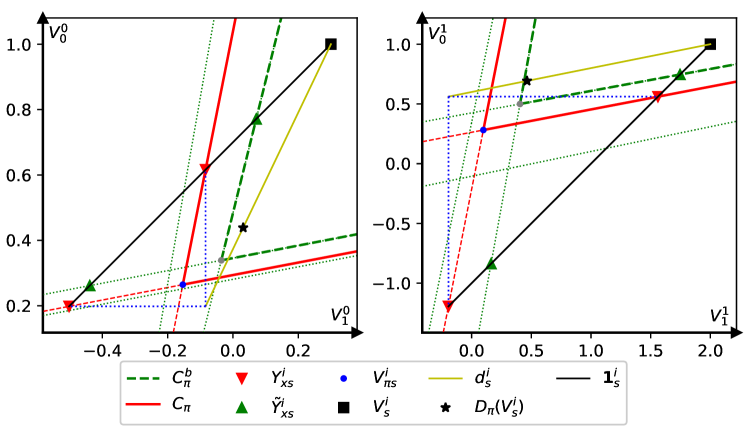
Figure 1: Graph of a policy cone and best response cone. This figure is plotted with a dynamic game with 2 players, 2 states, and 2 actions, that is, $N=\mathcal{S}=\mathcal{A}=\{0,1\}$. The graph is based on the value function space $\mathcal{V}$, where the two axes in each subfigure respectively represent two state indexes $s\in\{0,1\}$ of $V_{s}^{i}$, and the two subfigures respectively represent two player indexes $i\in\{0,1\}$ of $V_{s}^{i}$.

Proposition 1.

Let $\pi_{a}^{si}$ be a policy in dynamic game $\Gamma$, and then the following properties hold.

1. The unique solution $V_{\pi s}^{i}$ of $V_{\pi s}^{i}=D_{\pi}(V_{\pi s}^{i})$ satisfies $V_{\pi s}^{i}\in C_{\pi}$, and for any $V_{s}^{i}\in C_{\pi}$, $V_{s}^{i}\geq V_{\pi s}^{i}$.

2. For any $V_{s}^{i}\in\mathcal{V}$ and $x\in\mathcal{S}$, there exists an unique pair of $Y_{xs}^{i}\in\mathcal{V}$ and $d_{x}^{i}$ such that

   $$\left(Y_{xs}^{i}-D_{\pi}(Y_{xs}^{i})\right)(x)=0\wedge V_{s}^{i}-Y_{xs}^{i}=d_{x}^{i}\mathbf{1}_{s},$$ (1)

   as well as an unique pair of $\tilde{Y}_{xs}^{i}\in\mathcal{V}$ and $\tilde{d}_{x}^{i}$ such that

   $$\left(\tilde{Y}_{xs}^{i}-\max_{a}^{si}D_{\pi}^{i-}(\tilde{Y}_{xs}^{i})\right)(x)=0\wedge V_{s}^{i}-\tilde{Y}_{xs}^{i}=\tilde{d}_{x}^{i}\mathbf{1}_{s}.$$ (2)

3. For any $V_{s}^{i}\in\mathcal{V}$, there exists an $M>0$ such that for any $m>M$, $V_{s}^{i}+m\mathbf{1}_{s}^{i}\in C_{\pi}^{b}\subseteq C_{\pi}$.

According to Definition 3 and Proposition 1 (i), policy cone $C_{\pi}$ is a set indexed by $i\in N$ of cone-shaped regions, each surrounded by $\left\lvert\mathcal{S}\right\rvert$ hyperplanes in $\left\lvert\mathcal{S}\right\rvert$-dimensional value function space $\mathcal{V}$, with $V_{\pi s}^{i}$ being a set of their apexes, and best response cone $C_{\pi}^{b}$ is a subset of policy cone $C_{\pi}$, consists of a set indexed by $i\in N$ of intersects of $\left\lvert\mathcal{A}\right\rvert$ cone-shaped regions. In Fig. 1, policy $\pi_{a}^{si}$ is represented by policy cone $C_{\pi}$ and best response cone $C_{\pi}^{b}$. $C_{\pi}$ is the two cone-shaped regions surrounded by red lines in each subfigure, where red dashed lines are the corresponding hyperplanes. $C_{\pi}^{b}$ is the two regions surrounded by green dashed lines in each subfigure, where green dotted lines are the corresponding hyperplanes that intersect and surround it. The set of apexes $V_{\pi s}^{i}$ is represented by blue point markers.

Proposition 1 (ii) and (iii) show that both bottoms of $C_{\pi}$ and $C_{\pi}^{b}$ expand towards infinity along $\mathbf{1}_{s}^{i}$, and there is always an unique intersection $Y_{xs}^{i}$ between each hyperplane indexed by $x$ and $i$ of $C_{\pi}$ and the line in direction $\mathbf{1}_{s}^{i}$ passing through $V_{s}^{i}\in\mathcal{V}$, and the same goes for $\tilde{Y}_{xs}^{i}$ and $C_{\pi}^{b}$. It can be seen in Fig. 1 how the bottoms of $C_{\pi}$ and $C_{\pi}^{b}$ expand and how the line $\mathbf{1}_{s}^{i}$ intersects with $C_{\pi}$ and $C_{\pi}^{b}$, where $V_{s}^{i}\in\mathcal{V}$ is represented by black square markers, $\mathbf{1}_{s}^{i}$ is represented by black lines, the unique intersections $Y_{xs}^{i}$ and $\tilde{Y}_{xs}^{i}$ are represented by red triangle down markers and green triangle up markers respectively. With the core concept of policy cone and best response cone, we next give two theorems bridging dynamic programming operator and perfect equilibrium.

Theorem 2 (Iterative properties).

Let $\pi_{a}^{si}$ be a policy in dynamic game $\Gamma$, and then the following properties of dynamic programming operator $D_{\pi}$ hold.

1. $V_{s}^{i}\geq D_{\pi}(V_{s}^{i})$ if and only if $V_{s}^{i}\in C_{\pi}$.

2. For any $V_{s}^{i}\in C_{\pi}$, $D_{\pi}(V_{s}^{i})\in C_{\pi}$.

3. For any $V_{s}^{i}\in C_{\pi}$, $D_{\pi}(V_{s}^{i})\in C_{\pi}^{b}$, if and only if $\pi_{a}^{si}=\arg\max_{a}^{si}D_{\pi}^{i-}(V_{s}^{i})$.

4. For any $V_{s}^{i}\in C_{\pi}$, the residual

   $$V_{s}^{i}-D_{\pi}(V_{s}^{i})= (1-\gamma)d_{s}^{i},$$

   $$V_{s}^{i}-\max_{a}^{si}D_{\pi}^{i-}(V_{s}^{i})= (1-\gamma)\tilde{d}_{s}^{i},$$

   where $d_{s}^{i}$ and $\tilde{d}_{s}^{i}$ are given by formula (1) and (2) respectively.

5. Let $V_{s}^{i}$ iterates by $V_{s,k+1}^{i}=D_{\pi}(V_{s,k}^{i})+m\mathbf{1}_{s}^{i}$, where $m>0$ is a constant, and initial value function $V_{s,0}^{i}\in C_{\pi}$. Then

   $$\lim_{k\to\infty}V_{s,k}^{i}=V_{\pi s}^{i}+\frac{m}{1-\gamma}\mathbf{1}_{s}^{i},$$

   $$\lim_{k\to\infty}\tan\measuredangle\left(V_{s,k}^{i}-D_{\pi}(V_{s,k}^{i}),\mathbf{1}_{s}^{i}\right)=0.$$

Theorem 3 (Equilibrium conditions).

The following equivalent conditions of equilibrium hold.

1. $\pi_{a}^{si}$ is a perfect equilibrium if and only if $V_{\pi s}^{i}\in C_{\pi}^{b}$.

2. Given value function $V_{s}^{i}$, for any $x\in\mathcal{S}$, $\pi_{a}^{si}(x)$ is a Nash equilibrium of the static game with utility function $(u_{A}^{si}+\gamma T_{s^{\prime}A}^{s}V_{s^{\prime}}^{i})(x)$ if and only if $Y_{xs}^{i}=\tilde{Y}_{xs}^{i}$, where $Y_{xs}^{i}$ and $\tilde{Y}_{xs}^{i}$ are given by formula (1) and (2) respectively.

Theorem 2 uses policy cone $C_{\pi}$ and best response cone $C_{\pi}^{b}$ to describe iterative properties of dynamic programming operator $D_{\pi}$ for fixed policy $\pi_{a}^{si}$. (i), (ii), and (iii) suggest that $C_{\pi}$ is the monotonic and closed domain for $D_{\pi}$, and $C_{\pi}^{b}$ is closed if and only if $\pi_{a}^{si}$ is a Nash equilibrium for every state. As in, for any iteration starting from value function $V_{s}^{i}$ within $C_{\pi}$, the value function decreases monotonically as iterates and never leaves $C_{\pi}$, which means the iteration converges to the apex $V_{\pi s}^{i}$ of $C_{\pi}$ by the monotone convergence theorem. (iv) illustrates that iteration residual $V_{s}^{i}-D_{\pi}(V_{s}^{i})$ of $D_{\pi}$ can be expressed by the distance $d_{x}^{i}$ pairing with the unique intersection $Y_{xs}^{i}$ described in Proposition 1 (ii), where the set indexed by state $x$ of distances $d_{x}^{i}$ is used as a single vector $d_{s}^{i}$, and the same goes for $\max_{a}^{si}D_{\pi}^{i-}$, $\tilde{d}_{x}^{i}$, and $\tilde{Y}_{xs}^{i}$. In Fig. 1, it can be seen how $d_{x}^{i}$ is paired with $Y_{xs}^{i}$ by blue dotted lines as Proposition 1 (ii) shows, and how the residual satisfies $V_{s}^{i}-D_{\pi}(V_{s}^{i})=(1-\gamma)d_{s}^{i}$ as Theorem 2 (iv) shows, where $d_{s}^{i}$ is represented by yellow lines, and $D_{\pi}(V_{s}^{i})$ is represented by black star markers. In addition to value function $V_{s}^{i}$ iteratively converging to apex $V_{\pi s}^{i}$, (v) shows that if a scaled $\mathbf{1}_{s}^{i}$ is added in every iteration, not only does $V_{s}^{i}$ converge to $V_{\pi s}^{i}$ adding a scaled $\mathbf{1}_{s}^{i}$, but $V_{s}^{i}-D_{\pi}(V_{s}^{i})$ also converge to a scaled $\mathbf{1}_{s}^{i}$.

Theorem 3 uses $C_{\pi}$ and $C_{\pi}^{b}$ to describe sufficient and necessary conditions of equilibriums. (ii) shows that policy $\pi_{a}^{si}$ is a Nash equilibrium for state $x$ if and only if the unique intersects $Y_{xs}^{i}$ and $\tilde{Y}_{xs}^{i}$ coincide for state $x$, that is, the corresponding pair of red triangle down marker and green triangle up marker coincide in Fig. 1. (i) shows that policy $\pi_{a}^{si}$ is a perfect equilibrium if and only if the apex $V_{\pi s}^{i}$ of $C_{\pi}$ is in $C_{\pi}^{b}$, that is, the blue point marker coincides with the gray marker on $C_{\pi}^{b}$ in Fig. 1. And at this time, all the markers in the graph coincide, which may also be interpreted as not only do $Y_{xs}^{i}$ and $\tilde{Y}_{xs}^{i}$ coincide to imply a Nash equilibrium for every state, but they also coincide with the apex $V_{\pi s}^{i}$ to imply value function $V_{s}^{i}$ corresponding with policy $\pi_{a}^{si}$.

These two theorems build a bridge between the dynamic programming operator and the perfect equilibrium, where Theorem 2 points out a method for dynamic programming operator $D_{\pi}$ to iteratively converge, and Theorem 3 points out equivalent conditions for the convergence point to be a perfect equilibrium value function. Thus, we next study the possibility for a iterative method constructed by dynamic programming operator $D_{\pi}$ to converge to a perfect equilibrium.

Proposition 4.

Let $V_{s}^{i}$ iterates by $V_{s,k+1}^{i}=D(V_{s,k}^{i}):=D_{\pi_{k}}(V_{s,k}^{i})$, where $\pi_{a,k}^{si}=\arg\max_{a}^{si}D_{\pi_{k}}^{i-}(V_{s,k}^{i})$. If $V_{s,0}^{i}\in C_{\pi_{0}}$, then the following statements satisfy $(i)\Rightarrow(ii)\Rightarrow(iii)\Leftrightarrow(iv)$.

1. $V_{s}^{i}\leq Y_{s}^{i}\rightarrow D(V_{s}^{i})\leq D(Y_{s}^{i})$ for every $V_{s}^{i},Y_{s}^{i}\in O(\hat{V}_{s}^{i})$, where $O(\hat{V}_{s}^{i})$ is a set such that $V_{s,k}^{i}\in O(\hat{V}_{s}^{i})$ for all $k$.

2. $V_{s,k}^{i}$ converges to a perfect equilibrium value function by contraction mapping $D$, and $V_{s,k}^{i}\in C_{\pi_{k}}$ for all $k$.

3. $V_{s,k}^{i}$ monotonically converges to a perfect equilibrium value function.

4. $V_{s,k+1}^{i}\leq V_{s,k}^{i}\rightarrow D(V_{s,k+1}^{i})\leq D(V_{s,k}^{i})$ for all $k$.

Using Theorem 2 (iii), it can be inferred that Proposition 4 (iv) is equivalent to $V_{k+1}\in C_{\pi_{k}}^{b}\rightarrow V_{k+1}\in C_{\pi_{k+1}}$. It can be verified on the graph of policy cone and best response cone that this implication formula generally does’t hold, since $\pi_{k}$ and $\pi_{k+1}$ generally doesn’t have a strong relation. Consequently, none of the four statements hold in dynamic games. In particular, neither does the first half of (ii) that operator $D$ is a contraction mapping hold on its own, since previous research already shows that operator $D$ fails to converge in dynamic games[11, 12]. However, as the degeneration of operator $D$ in dynamic games into where there is only one player, the Bellman operator $D$ in MDPs satisfies (i), which can be used to prove the first half of (ii) that Bellman operator $D$ is a contraction mapping. Furthermore, if there is also $V_{s,0}^{i}\in C_{\pi_{0}}$ for Bellman operator $D$, then all the four statements hold as Proposition 4 shows, where perfect equilibrium degenerates to optimal policy. Proposition 4 is not necessary to construct our iterative approximation method in this paper. However, it provides a certain perspective why the Bellman operator and value iteration cannot be simply generalized to dynamic games.

Theorem 5 (Cone interior convergence conditions).

Let $V_{s}^{i}$ iterates by

$$V_{s,k+1}^{i}=D_{\pi_{k}}(V_{s,k}^{i}+m_{k}\mathbf{1}_{s}^{i}),$$

where $\{\pi_{a,k}^{si}\}_{k\in\mathbb{N}}$ is a sequence of policies such that $\lim_{k\to\infty}\pi_{a,k}^{si}=\hat{\pi}_{a}^{si}$, and $\{m_{k}\}_{k\in\mathbb{N}}$ is a sequence of scalars. Then $V_{s,k}^{i}$ converges to a perfect equilibrium value function if and only if

$$\lim_{k\to\infty}m_{k}=0\wedge\lim_{k\to\infty}m^{\prime}_{k}=0,$$

where $\{m^{\prime}_{k}\}_{k\in\mathbb{N}}$ is another sequence of scalars sufficiently large such that $V_{s,k}^{i}+m^{\prime}_{k}\mathbf{1}_{s}^{i}\in C_{\pi_{k}}^{b}$.

Theorem 5 points out a method that iteratively converges to a perfect equilibrium sufficiently and necessarily, where $m_{k}$ and $\pi_{k}$ are required in each iteration step. First, for simplification, let $m_{k}=m^{\prime}_{k}$, and thus $m_{k}$ only needs to be large enough so that $V_{s,k}^{i}+m_{k}\mathbf{1}_{s}^{i}\in C_{\pi_{k}}^{b}$. Second, $\pi_{a,k}^{si}$ needs to converge to a Nash equilibrium for every state, which is equivalent to $m_{k}$ and $m^{\prime}_{k}$ converging to $0$ as Theorem 2 (iii) points out. We use the method in the next section to iteratively approximate a Nash equilibrium to compute $\pi_{k}$. Finally, we might as well use the operator $\max_{a}^{si}D_{\pi_{k}}^{i-}$ for iteration because $\arg\max_{a}^{si}D_{\pi}^{i-}(V_{s}^{i})$ varies slower than $\pi_{a}^{si}$, resulting in a more robust iteration. According to its feature that the iterated value function by the dynamic programming operator always stays in the policy cone, we call this method cone interior dynamic programming.

3 Primal-dual unbiased regret minimization

In this section, our intention is to enable the polynomial-time line search method in local optimization to achieve convergence guarantee to Nash equilibriums of static games. We first give a regret minimization problem, followed by its KKT conditions and an unbiased condition that establish its equivalence to the Nash equilibrium, and then explain the key difference between our method and existing methods that guarantees the convergence of our method. Then we define the two core concepts of unbiased barrier problem and unbiased KKT conditions, as well as primal-dual bias and unbiased central path, followed by their graphs, and consequently come to a theorem establishing the equivalence between the unbiased central path and the conditions of perturbed KKT conditions and unbiased condition, as well as explaining the connection between our method and interior point methods. Finally, we give existence, projected gradient, tangent vector, starting point, and singular indication to search through the unbiased central path of which the end point is sufficiently and necessarily a Nash equilibrium.

This section mainly deals with static games. Thus unconventionally, we may drop the index $s$ when one state is referred and put it on when all states are referred, such as $\pi_{a}^{i}$ represents $\pi_{a}^{si}(x)$ for some state $x$. Then similar to the last section, for policy $\pi_{a}^{i}$, $\pi_{A}$ denotes $\left(\prod_{j\in N}\pi_{a_{j}}^{j}\right)_{A}$, $\pi_{Aa}^{i-}$ denotes $\left(I_{a_{i}a}\prod_{j\in N-\left\{i\right\}}\pi_{a_{j}}^{j}\right)_{Aa}^{i}$, and $\max_{a}^{i}$ represents the maximum with respect to $a$ for every index $i$. In addition, let $\pi_{Aaa^{\prime}}^{ij-}$ denote $\left(I_{a_{i}a}I_{a_{j}a^{\prime}}\prod_{k\in N-\left\{i,j\right\}}\pi_{a_{k}}^{k}\right)_{Aaa^{\prime}}^{ij}$. Finally, $\pi_{a}^{i}\circ r_{a}^{i}$ represents element-wise product with no summation.

Definition 4 (Regret minimization problem).

Let $G$ be a static game, where the utility function is $U:\prod_{i\in N}\mathcal{A}\to\prod_{i\in N}\mathbb{R}$. A regret minimization problem of $G$ is optimization problem (3) with $\mu_{a}^{i}=0$, where $(\pi_{a}^{i},r_{a}^{i},v^{i})$ is a tuple of policy, regret, and value, and $\mu_{a}^{i}$ is a barrier parameter.

$$\min_{(\pi_{a}^{i},r_{a}^{i},v^{i})} \pi_{a}^{i}r_{a}^{i}-\mu_{a}^{i}\ln r_{a}^{i}-\mu_{a}^{i}\ln\pi_{a}^{i}$$ (3)

s.t. $$r_{a}^{i}-v^{i}+\pi_{Aa}^{i-}U_{A}^{i}=0$$

$$\mathbf{1}_{a}\pi_{a}^{i}-\mathbf{1}^{i}=0$$

The case where $\mu_{a}^{i}\neq 0$ is a barrier problem of (3).

According to the purification theorem[13], $\pi_{a}^{i}$ is a Nash equilibrium if and only if for every player $i$, every action $a$ that satisfies $\pi_{a}^{i}>0$ has the same utility. Thus, mixed Nash equilibriums are not stable equilibrium points for any method based on optimizing the utility of the updated strategy, such as no-regret[14, 15] and self-play[16, 17]. There is a difference in the meaning of regret. The regret in no-regret methods is a vector of differences between the utility of the updated mixed strategy and the utilities of every action, while the regret in regret minimization problem (3) is a vector of differences between the maximum utility and the utilities of every action plus a scalar. The difference upon the quantity being optimized is why our method has convergence guarantee while existing methods based on no-regret or self-play don’t, and consequently exhibit non-stationarity in training when used in multi-agent reinforcement learning.

Theorem 6 (Unbiased condition).

Let $G$ be a static game and $(\pi_{a}^{i},r_{a}^{i},v^{i})$ be a tuple of policy, regret and value of $G$. Then the following statements are equivalent.

1. $(\pi_{a}^{i},v^{i})$ is a Nash equilibrium of $G$.

2. $(\pi_{a}^{i},r_{a}^{i},v^{i})$ is an optimal point of regret minimization problem (3).

3. There exist Lagrangian multipliers $(\bar{\lambda}_{a}^{i},\tilde{\lambda}^{i},\hat{\pi}_{a}^{i},\hat{r}_{a}^{i})$ satisfying two conditions, the KKT conditions shows by equation (4) with $\mu_{a}^{i}=0$ and unbiased condition $\pi_{a}^{i}=\hat{\pi}_{a}^{i}$.

   $$\begin{bmatrix}\bar{\lambda}_{a}^{j}\pi_{Aaa^{\prime}}^{ij-}U_{A}^{i}+\tilde{\lambda}^{i}\mathbf{1}_{a^{\prime}}+r_{a^{\prime}}^{i}-\hat{r}_{a^{\prime}}^{i}\\ \bar{\lambda}_{a}^{i}+\pi_{a}^{i}-\hat{\pi}_{a}^{i}\\ -\mathbf{1}_{a}\bar{\lambda}_{a}^{i}\\ r_{a}^{i}\circ\hat{\pi}_{a}^{i}-\mu_{a}^{i}\\ \pi_{a}^{i}\circ\hat{r}_{a}^{i}-\mu_{a}^{i}\\ r_{a}^{i}-v^{i}+\pi_{Aa}^{i-}U_{A}^{i}\\ \mathbf{1}_{a}\pi_{a}^{i}-\mathbf{1}^{i}\end{bmatrix}=0$$ (4)

Furthermore, when these statements hold, the objective function $\pi_{a}^{i}r_{a}^{i}$ of (3) is $0$, and $(\bar{\lambda}_{a}^{i},\tilde{\lambda}^{i},\pi_{a}^{i}-\hat{\pi}_{a}^{i},r_{a}^{i}-\hat{r}_{a}^{i})=0$.

Theorem 6 points out that the Nash equilibrium is not only equivalent to the global optimal point of regret minimization problem (3), but also to its local extreme point satisfying the unbiased condition, where the local extreme point is equivalent to the point satisfying KKT conditions[18] in (iii). In previous research[19, 20], linear programming, quadratic programming, linear complementarity problem, and Nash equilibrium of bimatrix games have been unified, and the unification is actually a degeneration of $(i)\Leftrightarrow(ii)$ into 2 player static games. $(i)\Leftrightarrow(ii)$ points out the connection between our method and existing methods, but not necessary in constructing our method. $(i)\Leftrightarrow(iii)$ makes it possible to use local optimization methods that can keep bias $\pi_{a}^{i}-\hat{\pi}_{a}^{i}$ at $0$ to compute global optimal points of (3), and equivalently Nash equilibriums.

Definition 5 (Unbiased barrier problem and primal-dual bias).

An unbiased barrier problem is the parameterized optimization problem

$$\begin{aligned} \min_{(\pi_{a}^{i},r_{a}^{i},v^{i})}\quad&\left(\pi_{a}^{i}-\hat{\pi}_{a}^{i}\right)\left(r_{a}^{i}-\hat{r}_{a}^{i}\right)\\ \textrm{s.t.}\quad&r_{a}^{i}-v^{i}+\pi_{Aa}^{i-}U_{A}^{i}=0\\ &\mathbf{1}_{a}\pi_{a}^{i}-\mathbf{1}^{i}=0\end{aligned},$$ (5)

where $\hat{\pi}_{a}^{i}=\mu_{a}^{i}/r_{a}^{i}$ and $\hat{r}_{a}^{i}=\mu_{a}^{i}/\pi_{a}^{i}$ are constant parameters called the dual policy and dual regret respectively. A primal-dual bias is a tuple $(\pi_{a}^{i}-\hat{\pi}_{a}^{i},r_{a}^{i}-\hat{r}_{a}^{i})$.

Definition 6 (Unbiased KKT conditions and unbiased central path).

Unbiased KKT conditions are simultaneous equations

$$\begin{bmatrix}\hat{\pi}_{a}^{i}\circ r_{a}^{i}-\mu_{a}^{i}\\ r_{a}^{i}-v^{i}+\pi_{Aa}^{i-}U_{A}^{i}\\ \mathbf{1}_{a}\hat{\pi}_{a}^{i}-\mathbf{1}^{i}\end{bmatrix}=0,$$ (6a)

$$\pi_{a}^{i}=\hat{\pi}_{a}^{i}.$$ (6b)

An unbiased central path is a map from $\mu_{a}^{i}$ to $\pi_{a}^{i}$ that satisfies unbiased KKT conditions.

The local optimization method we use is similar to interior point methods[21]. In interior point methods, a barrier problem is iteratively locally optimized as the barrier parameter decreases, and the local optimal point of the barrier problem forms a trajectory known as the central path, and the local optimal point of the orginal problem is at the end of the central path where the barrier parameter decreases to $0$. In our method, we aim to keep the updated point on central paths on which the primal-dual bias is $0$, namely the unbiased central path by next theorem. In order to achieve this, the updated point needs to only move an infinitesimal step everytime barrier parameter $\mu_{a}^{i}$ decreases by an infinitesimal step, due to the existence of biased local extreme points. Thus, we need two directions of updates, where we use unbiased barrier problem (5) to move onto the unbiased central path, and use unbiased KKT conditions (6) to move along the unbiased central path as barrier parameter $\mu_{a}^{i}$ decreases.

Theorem 7.

Given $\mu_{a}^{i}$, for the tuple $(\pi_{a}^{i},r_{a}^{i},v^{i})$, the following properties satisfy $(i)\Leftrightarrow(ii)\Leftrightarrow((iii)\wedge\pi_{a}^{i}=\hat{\pi}_{a}^{i})$ and $(iii)\Leftrightarrow(iv)\Leftrightarrow(v)$.

1. Being is a global optimal point of unbiased barrier problem (5).

2. Being a solution of unbiased KKT conditions (6).

3. Being a solution of perturbed KKT conditions (4) for some $(\bar{\lambda}_{a}^{i},\tilde{\lambda}^{i},\hat{\pi}_{a}^{i},\hat{r}_{a}^{i})$.

4. Being a local extreme point of unbiased barrier problem (5).

5. Being is a local extreme point of barrier problem (3).

There are two formulas in Theorem 7. The first one $(i)\Leftrightarrow(ii)\Leftrightarrow((iii)\wedge\pi_{a}^{i}=\hat{\pi}_{a}^{i})$ shows that the global optimal point of unbiased barrier problem (5), the solution of unbiased KKT conditions (6), and the solution of the simultaneous equations of perturbed KKT conditions (4) and unbiased condition $\pi_{a}^{i}=\hat{\pi}_{a}^{i}$ in Theorem 6 (iii) are equivalent, justifying our intention to use (5) and (6) to search through the unbiased central path. While the second one $(iii)\Leftrightarrow(iv)\Leftrightarrow(v)$ aims to illustrate the connection between our method and interior point methods, that is, the unbiased central path in Definition 6 really is the central path in interior point methods on which the primal-dual bias is $0$. In fact, our method is independent of interior point methods, and its feasibility is validated by the first formula, while the second formula is not necessary for the validation.

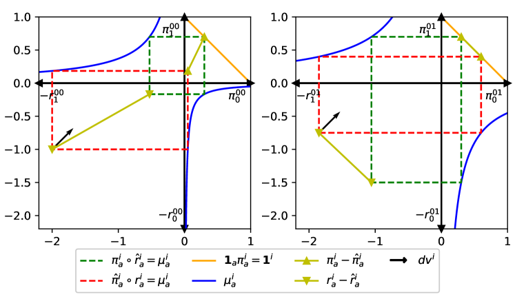
Figure 2: Graph of an unbiased barrier problem. This figure is plotted with the same dynamic game as Fig. 1. The graph is based on the joint space of policy $\pi_{a}^{si}$ and regret $r_{a}^{si}$. The positive half of the two axes in each subfigure respectively represent two action indexes $a\in\{0,1\}$ of policy $\pi_{a}^{i}$, the negitive half of the two axes in each subfigure respectively represent two action indexes $a\in\{0,1\}$ of regret $r_{a}^{i}$, and the two subfigures respectively represent two player indexes $i\in\{0,1\}$. Only one of the states $s=0$ is exhibited, omitting two subfigures corresponding to the other one $s=1$. Thus, policy $\pi_{a}^{i}$ and dual policy $\hat{\pi}_{a}^{i}$ are plotted on the all positive quadrant, and regret $r_{a}^{i}$ and dual regret $\hat{r}_{a}^{i}$ are plotted on the all negitive quadrant. Rotating the two action indexes of $r_{a}^{i}$, barrier parameter $\mu_{a}^{i}$ is plotted between positive half and negitive half of the axes as hyperbolas represented by blue curves. In this way, $\hat{\pi}_{a}^{i}\circ r_{a}^{i}=\mu_{a}^{i}$ and $\pi_{a}^{i}\circ\hat{r}_{a}^{i}=\mu_{a}^{i}$ have rectangular shapes represented by red and green dashed rectangles, and primal-dual bias $(\pi_{a}^{i}-\hat{\pi}_{a}^{i},r_{a}^{i}-\hat{r}_{a}^{i})$ is the bias of two rectangles represented by yellow lines with triangle up markers and triangle down markers.

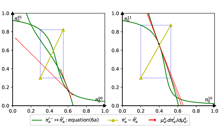
Figure 3: Graph of unbiased KKT conditions. This figure is plotted with the same dynamic game as Fig. 1. The graph is based on the policy space, where the two axes in each subfigure respectively represent two player indexes $i\in\{0,1\}$ of $\pi_{a}^{si}$, and the two subfigures respectively represent two state indexes $s\in\{0,1\}$ of $\pi_{a}^{si}$, and only one of the two action indexes $a=0$ is needed to represent $\pi_{a}^{si}$, since $\pi_{a}^{si}$ sums to $1$ over action indexes.

Theorem 8.

The following properties about unbiased barrier problem (5) and unbiased KKT conditions (6) hold.

1. For any $\pi_{a}^{i}$ and $\mu_{a}^{i}$, there exists an unique $v^{i}$ satisfying equation (6a).

2. If $\mathbf{1}_{a}\hat{\pi}_{a}^{i}-\mathbf{1}^{i}=0$, then the projected gradient of (5) is

   $${\rm pg}_{a^{\prime\prime}}^{j}:=\left(I_{a^{\prime}a^{\prime\prime}}-\frac{\mathbf{1}_{a^{\prime}}\mathbf{1}_{a^{\prime\prime}}}{\left\lvert\mathcal{A}\right\rvert}\right)\left(\left(r_{a^{\prime}}^{j}-\hat{r}_{a^{\prime}}^{j}\right)-\left(\pi_{a}^{i}-\hat{\pi}_{a}^{i}\right)\pi_{Aaa^{\prime}}^{ij-}U_{A}^{i}\right).$$ (7)

3. For every $\mu_{a}^{i}$, there is at least one solution $\pi_{a}^{i}$ of (6).

4. The solution $\pi_{a}^{i}$ of (6) for $\mu_{a}^{i}=\hat{\mu}_{a}^{i}\mu^{\prime}$ satisfies $\lim_{\mu^{\prime}\to+\infty}\pi_{a}^{i}=\hat{\mu}_{a}^{i}/(\mathbf{1}_{a}\hat{\mu}_{a}^{i})$.

5. The set of tangent vectors $\mu_{a^{\prime\prime}}^{k}d\pi_{a^{\prime}}^{j}/d\mu_{a^{\prime\prime}}^{k}$ on a solution $\pi_{a}^{i}$ of (6) for $\mu_{a}^{i}$ satisfies

   $$\begin{bmatrix}H_{(j,a^{\prime})}^{(i,a)}&B^{(i,a)}_{l}\\ B_{(j,a^{\prime})}^{m}&\mathbf{0}_{l}^{m}\end{bmatrix}\begin{bmatrix}\left(\frac{d\pi_{a^{\prime}}^{j}}{\pi_{a^{\prime}}^{j}d\mu_{a^{\prime\prime}}^{k}}\right)_{(k,a^{\prime\prime})}^{(j,a^{\prime})}\\ \left(\frac{dv^{l}}{d\mu_{a^{\prime\prime}}^{k}}\right)_{(k,a^{\prime\prime})}^{l}\end{bmatrix}=\begin{bmatrix}I_{(k,a^{\prime\prime})}^{(i,a)}\\ \mathbf{0}_{(k,a^{\prime\prime})}^{m}\end{bmatrix},$$ (8)

   where

   $$H_{(j,a^{\prime})}^{(i,a)}={\rm Diag}(\mu_{(i,a)})-\left(\pi_{a}^{i}\circ\pi_{Aaa^{\prime}}^{ij-}U_{A}^{i}\circ\pi_{a^{\prime}}^{j}\right)_{(j,a^{\prime})}^{(i,a)},$$

   $$B_{(i,a)}^{m}=\pi_{(i,a)}\circ\left(I^{im}\mathbf{1}_{a}\right)_{(i,a)}^{m}.$$

6. Let $(\tilde{\mu}_{a}^{i},\tilde{\pi}_{a}^{i})$ be a solution where the coefficient matrix of equation (8) is singular, and suppose there is only one zero eigenvalue. Let $\mu_{a}^{i}=\tilde{\mu}_{a}^{i}(1+\mu^{\prime})$ and $\pi_{a}^{i}$ be a solution of (6) for $\mu_{a}^{i}$ in the neighborhood of $\tilde{\pi}_{a}^{i}$, where the coefficient matrix of equation (8) is non-singular. Then for every index $(k,a^{\prime\prime})$, the set of tangent vectors satisfies

   $$\lim_{\mu^{\prime}\to 0}\mathcal{N}_{a^{\prime\prime}}^{k}:=\lim_{\mu^{\prime}\to 0}\left\lVert\frac{\mu_{a^{\prime\prime}}^{k}d\pi_{a^{\prime}}^{j}}{d\mu_{a^{\prime\prime}}^{k}}\right\rVert_{2,2}=+\infty,$$ (9)

   $$\lim_{\mu^{\prime}\to 0}\mathcal{O}_{a^{\prime\prime}}^{k}:=\lim_{\mu^{\prime}\to 0}\cos\measuredangle\left(\frac{\mu_{a^{\prime\prime}}^{k}d\pi_{a^{\prime}}^{j}}{d\mu_{a^{\prime\prime}}^{k}},\mathbf{1}_{a^{\prime\prime}}^{k}\frac{\mu_{a^{\prime\prime}}^{k}d\pi_{a^{\prime}}^{j}}{d\mu_{a^{\prime\prime}}^{k}}\right)=\pm 1,$$ (10)

   where the norm is $L_{2,2}$ norm.

Theorem 8 (i) have two perspectives of interpretation. First, (i) shows that there is an unique $v^{i}$ to let dual policy $\hat{\pi}_{a}^{i}$ satisfy constraint $\mathbf{1}_{a}\pi_{a}^{i}=\mathbf{1}^{i}$. In Fig. 2, constraint $\mathbf{1}_{a}\pi_{a}^{i}=\mathbf{1}^{i}$ is represented by orange lines, and the vector $dv^{i}$ is represented by black arrows at regret $r_{a}^{i}$. The right subfigure shows a case where $\hat{\pi}_{a}^{i}$ is on the orange line while the left subfigure shows the otherwise, where it is intuitive to see why there is an unique $v^{i}$ to let $\hat{\pi}_{a}^{i}$ satisfy the constraint. Based on this interpretation, (ii) shows that when $\mathbf{1}_{a}\hat{\pi}_{a}^{i}=\mathbf{1}^{i}$ is satisfied, $\pi_{a}^{i}-\hat{\pi}_{a}^{i}$ and $dv^{i}$ are orthogonal, which is reflected in the right subfigure of Fig. 2. At this time, the projected gradient of unbiased barrier problem (5) has an analytical expression as equation (7) shows, pointing out the direction to update onto the unbiased central path. Second, (i) shows that for every joint policy $\pi_{a}^{i-}$ apart from player $i$, there is an unique dual policy $\hat{\pi}_{a}^{i}$ satisfying (6a). Then the map from $\pi_{a}^{i-}$ to $\hat{\pi}_{a}^{i}$ forms a function by definition. In Fig. 3, this function is plotted as the green curves, and primal-dual bias $\pi_{a}^{i}-\hat{\pi}_{a}^{i}$ is also plotted. Based on this interpretation, (iii) asserts the existence of the unbiased central path, that is, the green curves in Fig. 3 have at least one intersection, and the intersection is the point on the unbiased central path for current $\mu_{a}^{i}$. Theorem 8 (iv) shows that the starting point of the unbiased central path is determined by the initial value of barrier parameter $\mu_{a}^{i}$. The set of tangent vectors $\mu_{a^{\prime\prime}}^{k}d\pi_{a^{\prime}}^{j}/d\mu_{a^{\prime\prime}}^{k}$ in (v) points out the direction to update along the unbiased central path. In Fig. 3, the tangent vectors are represented by red arrows at the unbiased policy, that is, the intersection of the green curves.

Note that we mentioned that in order to keep the updated point on the unbiased central path, the updated point needs to only move an infinitesimal step everytime barrier parameter $\mu_{a}^{i}$ decreases by an infinitesimal step, so that we can always update back onto the unbiased central path after deviating with a step along the tangent vector. But this intention is attainable only when the coefficient matrix of equation (8) is non-singular, otherwise there are singular points on the unbiased central path that jams update. Considering only the case where there is only one zero eigenvalue, which is almost all the cases, (vi) points out the indication of singular points is that all the tangent vectors grow infinite long and contract to a 1D line. This property implies a singular avoidance procedure, which is introduced in the next section. In Fig. 3, the right subfigure shows a case where update is jammed by a singular point.

Regarding the unbiased central path, Theorem 8 shows its existence, projected gradient, tangent vector, starting point, and singular indication, and Theorem 7 shows that its end point is sufficiently and necessarily a primal-dual unbiased local extreme point of regret minimization problem (3), and equivalently a Nash equilibrium by Theorem 6 (iii). According to its feature, we call this method primal-dual unbiased regret minimization.

4 PTAS for perfect equilibriums of dynamic games

In this section, we first combine the two parts to give a complete structural framework of our method, including the singular avoidance module left in the last section, followed by the discussion on its time complexity. Then we exhibit some experimental results, including an iteration curve, an animation of the update process, and a test of universal effectiveness. Finally, we introduce the theoretical framework of our theory with existing theories and the potential to develop a model-free reinforcement learning method.

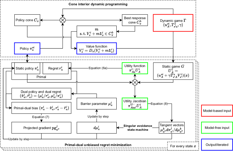
Figure 4: Structural framework. The computational flow graph of cone interior dynamic programming, primal-dual unbiased regret minimization, and their combination, where boxes represent quantities, arrows represent computations between quantities, and the computations all come from the theorems in the previous two sections. The framework takes dynamic game $\Gamma$ as input, or takes utility function $\pi_{Aa}^{i-}U_{A}^{i}$ and utility Jacobian $\pi_{Aaa^{\prime}}^{ij-}U_{A}^{i}$ in every iteration as a model-free alternative, and outputs the iteratively converged policy and value function as the perfect equilibrium and the corresponding value function.

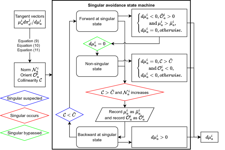
Figure 5: Singular avoidance state machine. The procedure to identify a singular point in advance and bypass it with backward and forward update, where rectangular boxes represent quantities, rounded boxes represent states, and diamonds represent state transitions. It takes the collinearity, orients, and norms of tangent vectors $\mu_{a}^{i}d\pi_{a^{\prime}}^{j}/d\mu_{a}^{i}$ as input and outputs the update step $d\mu_{a}^{i}$ of barrier parameter that can bypass the potential singular point.

$$\mathcal{C}:= \begin{aligned} \max_{c_{a^{\prime}}^{j}}\quad&\sqrt{\left\lVert\frac{\mu_{a}^{i}d\pi_{a^{\prime}}^{j}}{d\mu_{a}^{i}}c_{a^{\prime}}^{j}\right\rVert_{2,2}^{2}\bigg{/}\left(\left\lVert\frac{\mu_{a}^{i}d\pi_{a^{\prime}}^{j}}{d\mu_{a}^{i}}\right\rVert_{2,2}^{2}\mathbf{1}_{a}^{i}\right)}\\ \textrm{s.t.}\quad&\left\lVert c_{a^{\prime}}^{j}\right\rVert_{2,2}=1\\ \end{aligned}$$ (11)

$$= \sqrt{\theta_{\rm max}^{2}\bigg{/}\left(\left\lVert\frac{\mu_{a}^{i}d\pi_{a^{\prime}}^{j}}{d\mu_{a}^{i}}\right\rVert_{2,2}^{2}\mathbf{1}_{a}^{i}\right)}$$

Fig. 4 and Fig. 5 shows the structural framework of the combined iterative approximation method, including the singular avoidance procedure. In Fig. 5, the occurrence of singular points is determine by $\mathcal{C}$ exceeding threshold $\bar{C}$ and $\mathcal{N}_{a}^{i}$ all increasing, where $\mathcal{C}$ measures the degree of collinearity of the tangent vectors as equation (11) shows, and $\mathcal{N}_{a}^{i}$ and $\mathcal{O}_{a}^{i}$ are as equation (9) and equation (10) shows. In equation (11), similar to PCA (principal component analysis)[22], $\mathcal{C}$ maximize the averaged projected length of the tangent vectors on unit vector $c_{a^{\prime}}^{j}$, where $\theta_{\rm max}^{2}$ is the maximum squared singular value of matrix $(\mu_{a}^{i}d\pi_{a^{\prime}}^{j}/d\mu_{a}^{i})_{(i,a)}^{(j,a^{\prime})}$. The value of $\mathcal{C}$ lies in $[0,1]$, it can be interpreted as the maximum cosine of averaged angles between the tangent vectors and $c_{a^{\prime}}^{j}$. Three states in Fig. 5 respectively correspond to three update directions about $d\mu_{a}^{i}$. On the non-singular state, normally all components of $\mu_{a}^{i}$ decrease, unless $\mathcal{C}>\bar{C}$ occurs, indicating that there might be a singular point ahead. At this point, update $d\mu_{a}^{i}=0$ when $\mathcal{C}>\bar{C}\wedge\mathcal{O}_{a}^{i}<0$ is to facilitate the occurrence of a singular point if there is one, so that the signs of $\mathcal{O}_{a}^{i}$ are stablized and the singular avoidance procedure can proceed. Otherwise, if there is no singular point ahead, $\mathcal{C}$ would reduce in the process. The state transits to the backward at singular state when the indicator for singular points are met. At this point, $\mu_{a}^{i}$ and $\mathcal{O}_{a}^{i}$ are recorded, and then all components of $\mu_{a}^{i}$ increase such that $d\mu_{a}^{i}>0$, reducing $\mathcal{C}$ in the process. The state transits to the forward at singular state when $\mathcal{C}$ reduces below threshold $\bar{C}$. At this point, only the recorded positive oriented components such that $\bar{\mathcal{O}}_{a}^{i}>0$ of $\mu_{a}^{i}$ decrease, where the condition $\mu_{a}^{i}>\bar{\mu}_{a}^{i}$ is to determine whether the singular point is bypassed. The state transits back to the non-singular state when the bypassed condition is met.

This singular avoidance procedure is feasible due to two facts. First, the backward and forward update causes $\mu_{a}^{i}$ corresponding to orient $\mathcal{O}_{a}^{i}>0$ to decrease and $\mu_{a}^{i}$ corresponding to orient $\mathcal{O}_{a}^{i}<0$ to increase, resulting in the sideways movement of $\pi_{a}^{i}$ about the singular point. Second, note that there must be another solution apart from the singular point at $\mu_{a}^{i}$ according to Theorem 8 (iii), and the sideways movement actually leads $\pi_{a}^{i}$ to this other solution and eventually bypasses the current singular point. As in, $\mu_{a}^{i}$ eventually goes back to the recorded singular barrier parameter $\bar{\mu}_{a}^{i}$ in the process of backward and forward update, and $\pi_{a}^{i}$ shifts from the singular point to this other solution. This behavior is reflected in the animation of the update process attached to this paper.

The time complexity of this combined method is $O(\left\lvert\mathcal{S}\right\rvert^{m}\left\lvert\mathcal{A}\right\rvert^{n}\left\lvert N\right\rvert^{p}f(1/\mu_{a}^{si}))$, where $\mu_{a}^{si}$ measures the precision approximating a perfect equilibrium. Thus, this method is of polynomial-time with respect to the scale of state space $\mathcal{S}$, action space $\mathcal{A}$, and player set $N$. But due to the existence of singular points, $f(1/\mu_{a}^{si})$ is generally not a polynomial. In existing research, it has been proved that the problem of exactly computing a Nash equilibrium of a static game is in PPAD complexity class. For approximate computation methods, it has been proved that FPTAS (fully polynomial-time approximation scheme) does not exist for this problem unless PPAD itself is of polynomial-time, and whether PTAS exists remains an open question, where FPTAS requires further that $f(1/\mu_{a}^{si})$ is a polynomial on base of PTAS[2]. Not only for Nash equilibriums of static games, but also for perfect equilibriums of dynamic games, our method is a PTAS and not a FPTAS.

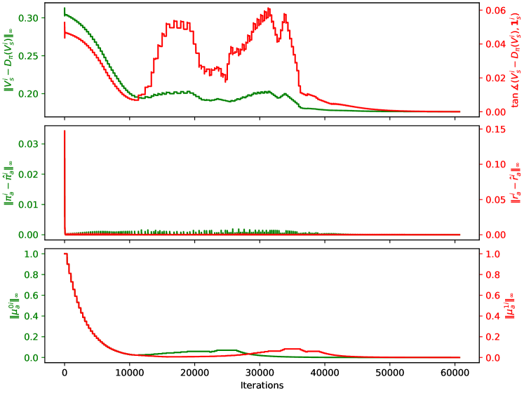
Figure 6: Iteration curve. Changes in the quantities used to measure the convergence corresponding to the three core concepts over iterations. Residual $V_{s}^{i}-D_{\pi}(V_{s}^{i})$ and its angle with $\mathbf{1}_{s}^{i}$ measures the convergence to apex of policy cone. Primal-dual bias $(\pi_{a}^{si}-\hat{\pi}_{a}^{si},r_{a}^{si}-\hat{r}_{a}^{si})$ measures the convergence onto unbiased central path. Barrier parameter $\mu_{a}^{si}$ measures the convergence along unbiased central path to its end point.

We tested our method on 2000 randomly generated dynamic games of 3 players, 3 states, and 3 actions in experiment, and the iteration converges to a perfect equilibrium on every single case, and there is only one threshold $\bar{C}$ in our implementation that needs to be adjusted as a hyperparameter for some rarely extreme cases. Note that the scale of 2 players, 2 states, and 2 actions is the largest scale for the three core concepts to be plotted on 2D plane like Fig. 1, Fig. 2, and Fig. 3. So we choose a dynamic game of this scale to plot the iteration curves in Fig. 6 and animate the update process based on the three core concepts to attach to this paper. In Fig. 6, residual $V_{s}^{i}-D_{\pi}(V_{s}^{i})$ and primal-dual bias $\pi_{a}^{si}-\hat{\pi}_{a}^{si}$ all converge to $0$ as barrier parameter $\mu_{a}^{si}$ converges to $0$. Thus, $\pi_{a}^{si}$ converges to a perfect equilibrium and $V_{s}^{i}$ converges to its value function by the theorems in the previous two sections. And primal-dual bias $(\pi_{a}^{i}-\hat{\pi}_{a}^{i},r_{a}^{i}-\hat{r}_{a}^{i})$ does stay at $0$ for the whole time as intended. Note that there is a fluctuation in both $\mu_{a}^{0i}$ and $\mu_{a}^{1i}$, because we choose a case where there is a singular point in both two states, and the fluctuations are signs of singular avoidance that causes $\mu_{a}^{i}$ to go backward and forward. Note also that singular avoidance also causes residual $V_{s}^{i}-D_{\pi}(V_{s}^{i})$ and its angle with $\mathbf{1}_{s}^{i}$ to fluctuate as $\mu_{a}^{i}$ increases, becaues value function $V_{s}^{i}$ converges faster under the iteration of operator $D_{\pi}$ parameterized by $\pi_{a}^{si}$ than $\pi_{a}^{si}$ itself, so the fluctuation may pass from $\pi_{a}^{si}$ to $V_{s}^{i}$. The animation of the update process attached to this paper is the union of Fig. 1, Fig. 2, and Fig. 3, corresponding to the update process of three major quantities, value function $V_{s}^{i}$, regret $r_{a}^{si}$, and policy $\pi_{a}^{si}$. All the above behaviors are reflected in the animation.

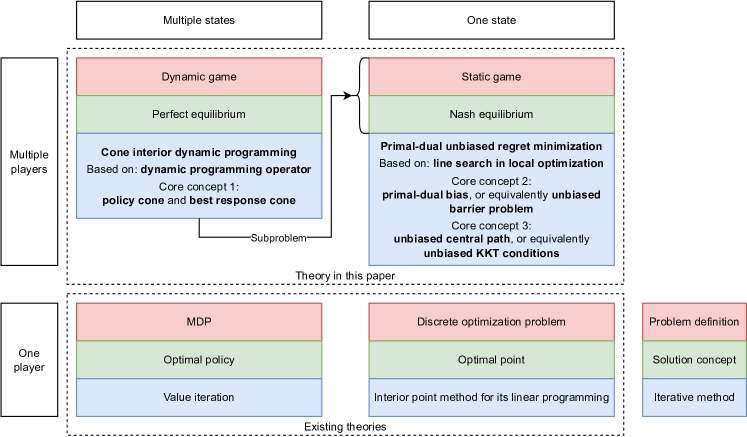
Figure 7: Theoretical framework. Theoretical framework of cone interior dynamic programming, primal-dual unbiased regret minimization, and their degeneration into existing theories as the dynamic game degenerates into the one player case or the one state case.

Note that in structural framework Fig. 4, even without the dynamic game as input, the utility function and utility Jacobian in the green boxes are enough to drive the whole computational flow, and it is possible to estimate these two quantities from sampled data collected when an agent plays a dynamic game instance, as an analogy with model-free methods in reinforcement learning like Q-learning[23]. Thus, it is possible to develop model-free reinforcement learning methods for dynamic games out of this PTAS, considering that current methods have the problem of non-stationarity in training and curse of dimensionality. Finally, there is a deep connection between the theory in this paper and existing theories of discrete optimization, game theory, and optimal control as Fig. 7 shows. Note that Q-learning in reinforcement learning is the combination of value iteration and stochastic approximation[24], so it is possible to analogically develop a Q-learning method for dynamic games out of this PTAS.

Our theory has a deep connection with the training of agents in model-free multi-agent reinforcement learning. The cone interior dynamic programming deals with the characteristics of dynamic and perfectness, by using dynamic programming operator $D_{\pi}(V_{s}^{i})=\pi_{A}^{s}(u_{A}^{si}+\gamma T_{s^{\prime}A}^{s}V_{s^{\prime}}^{i})+m\mathbf{1}_{s}^{i}$ to iterate value function $V_{s}^{i}$. Value function $V_{s}^{i}$ evaluates the long-term expected utility the agents expect about every state $s$. In training, agents estimate a new value function using the utility $u_{A}^{si}$ received from the environment and the long-term expected utility $\gamma T_{s^{\prime}A}^{s}V_{s^{\prime}}^{i}$, according to the policy $\pi_{a}^{si}$ used to interact with the environment, and then adjust the value function with a sufficiently large scalar $m$ to make themselves more optimistic about the long-term expected utility of every state. This adjustment $m$ may also encourage agents to explore the states uniformly in training. The perfectness is achieved when optimism level $V_{s}^{i}-D_{\pi}(V_{s}^{i})$ converges to $m\mathbf{1}_{s}^{i}$, that is, the agents become equally optimistic about all the states. The primal-dual unbiased regret minimization deals with the characteristics of game and equilibrium, by using utility function $\pi_{Aa}^{i-}U_{A}^{i}$ to compute the regret $r_{a}^{i}$ and utility Jacobian $\pi_{Aaa^{\prime}}^{ij-}U_{A}^{i}$ to update the policy $\pi_{a}^{i}$ and reduce total regret $\pi_{a}^{i}\circ r_{a}^{i}=\mu_{a}^{i}$, where $U_{A}^{i}=(u_{A}^{si}+\gamma T_{s^{\prime}A}^{s}V_{s^{\prime}}^{i})(x)$ for some state $x$. Regret $r_{a}^{i}$ evaluates the differences between the maximum utility $\max_{a}^{i}\pi_{Aa}^{i-}U_{A}^{i}$ and utilities of every action $a$ of agents, plusing a scalar to normalize dual policy $\mu_{a}^{i}/r_{a}^{i}$. This scalar may also encourage agents to explore the actions uniformly in training when total regret $\mu_{a}^{i}$ remains large. In training, agents estimate the utility function $\pi_{Aa}^{i-}U_{A}^{i}$ using their own sampled data and estimate utility Jacobian $\pi_{Aaa^{\prime}}^{ij-}U_{A}^{i}$ using the joint sampled data of all the agents, and then compute the projected gradient ${\rm pg}_{a^{\prime}}^{j}$ and tangent vector $\mu_{a}^{i}d\pi_{a^{\prime}}^{j}/d\mu_{a}^{i}$ to update policy $\pi_{a}^{i}$ according to the intended reduction $d\mu_{a}^{i}$ of total regret. The equilibrium is achieved when total regret $\pi_{a}^{i}\circ r_{a}^{i}=\mu_{a}^{i}$ reduces to $0$, that is, agents have zero regret about the actions they choose with non-zero probability. In summary, the model-free multi-agent reinforcement learning method developed from this PTAS would be a polynomial-time method that is free from non-stationarity in training and curse of dimensionality. The sufficiency and necessity means that regarding methods for perfect equilibriums of dynamic games based on dynamic programming and total regret minimization, a method constructed by our theory is sufficiently a PTAS, and conversely a method that is PTAS also necessarily has the same iteration process described by our theory, which means that our theory implies a certain unique PTAS for perfect equilibriums of dynamic games.

5 Conclusion

In this paper, we introduce our theory that consists of cone interior dynamic programming and primal-dual unbiased regret minimization, by which we construct our method and prove the sufficiency and necessity for the method to be the PTAS for perfect equilibriums of dynamic games. In cone interior dynamic programming, through the core concept of policy cone and best response cone, we obtain the sufficient and necessary condition for the polynomial-time dynamic programming operator to iteratively converge to a perfect equilibrium, leaving a subproblem equivalent to computing Nash equilibriums of static games. In primal-dual unbiased regret minimization, through the core concepts of primal-dual bias and unbiased central path, we establish the equivalence between the Nash equilibrium and the unbiased central path, and through the equivalent core concepts of unbiased barrier problem and unbiased KKT conditions, we obtain a projected gradient and linear equation based polynomial-time line search method to search through the unbiased central path, and equivalently approximate a Nash equilibrium. Regarding the three core concepts, we give the graphs of them and an animation of the update process based on them to visually illustrate the thoerems and our method. Universal effectiveness of our method is experimentally validated on numerous randomly generated dynamic games. With these cross-corroborating evidence, we come to the conclusion that our discovery of the PTAS for perfect equilibriums of dynamic games is sufficient and necessary, and the long-standing open question has been completed. In addition, our theory is consistent with existing theories and have an interface to develop a model-free multi-agent reinforcement learning method that is free from non-stationarity in training and curse of dimensionality. Also, the sufficiency and necessity in our theory implies our method has a certain degree of uniqueness for the PTAS based on dynamic programming and regret minimization.

Proofs

Lemma 9.

Let $T_{\pi}$ be a matrix satisfying $T_{\pi}\geq 0$ and $T_{\pi}\mathbf{1}=\mathbf{1}$, and let $\gamma\in(0,1)$. Then

1. $(I-\gamma T_{\pi})$ is invertible.

2. The formula $(I-\gamma T_{\pi})X\geq 0\rightarrow X\geq 0\rightarrow(\gamma T_{\pi})X\geq 0$ holds.

Proof.

(i) The eigenvalues of $(I-\gamma T_{\pi})$ is given by $1-\gamma\lambda_{i}$, where $\lambda_{i}$ are the eigenvalues of $T_{\pi}$. Note that inequality

$$T_{\pi}X\leq\max(X)$$

holds, and thus for real eigenvalue $\lambda_{i}$ that $T_{\pi}X=\lambda_{i}X$, we have $\lambda_{i}\leq 1$, and then $1-\gamma\lambda_{i}>0$. Hence $(I-\gamma T_{\pi})$ has no zero eigenvalues, and it’s invertible.

(ii) From $T_{\pi}\geq 0$ and $\gamma\in(0,1)$, we obtain $X\geq 0\rightarrow(\gamma T_{\pi})X\geq 0$. Note that inequality

$$T_{\pi}X\geq\min(X)$$

holds, and it follows that

$$\min((I-\gamma T_{\pi})X)\leq\min(X)-\gamma\min(T_{\pi}X)\leq(1-\gamma)\min(X).$$

Hence we obtain $(I-\gamma T_{\pi})X\geq 0\rightarrow X\geq 0$. ∎

Denote $T_{\pi s^{\prime}}^{s}:=\pi_{A}^{s}T_{s^{\prime}A}^{s}$ and $u_{\pi}^{si}:=\pi_{A}^{s}u_{A}^{si}$. As a corollary of Lemma 9 (i), there is an unique value function $V_{\pi s}^{i}=(I_{s^{\prime}}^{s}-\gamma T_{\pi s^{\prime}}^{s})^{-1}u_{\pi}^{s^{\prime}i}$ satisfying $V_{\pi s}^{i}=\pi_{A}^{s}(u_{A}^{si}+\gamma T_{s^{\prime}A}^{s}V_{\pi s^{\prime}}^{i})$ for any policy $\pi_{a}^{si}$.

Proof of Proposition 1.

(i) By definition of $V_{\pi s}^{i}$ and $C_{\pi}$, we obtain $V_{\pi s}^{i}\in C_{\pi}$. It follows from $V_{s}^{i}\in C_{\pi}$ that

$$\left(I_{s^{\prime}}^{s}-\gamma T_{\pi s^{\prime}}^{s}\right)\left(V_{s}^{i}-V_{\pi s}^{i}\right)=V_{s}^{i}-\pi_{A}^{s}\left(u_{A}^{si}+\gamma T_{s^{\prime}A}^{s}V_{s^{\prime}}^{i}\right)\geq 0.$$

Then by Lemma 9 (ii), we have $V_{s}^{i}-V_{\pi s}^{i}\geq 0$, and thus for all $V_{s}^{i}\in C_{\pi}$, $V_{s}^{i}\geq V_{\pi s}^{i}$.

(ii) Considering $V_{s}^{i}-Y_{xs}^{i}=d_{x}^{i}\mathbf{1}_{s}$, there is

$$\left(Y_{xs}^{i}-D_{\pi}(Y_{xs}^{i})\right)(x)=\left(V_{s}^{i}-D_{\pi}(V_{s}^{i})-(1-\gamma)d_{x}^{i}\mathbf{1}_{s}\right)(x).$$

Then let $d_{x}^{i}=(V_{s}^{i}-D_{\pi}(V_{s}^{i}))/(1-\gamma)$, and thus formula (1) is satisfied for every $x\in\mathcal{S}$. Note that $d_{x}^{i}$ is unique, and hence $Y_{xs}^{i}$ is unique.

Similarly, considering $V_{s}^{i}-\tilde{Y}_{xs}^{i}=\tilde{d}_{x}^{i}\mathbf{1}_{s}$, there is

$$\left(\tilde{Y}_{xs}^{i}-\max_{a}^{si}D_{\pi}^{i-}(\tilde{Y}_{xs}^{i})\right)(x)=\left(V_{s}^{i}-\max_{a}^{si}D_{\pi}^{i-}(V_{s}^{i})-(1-\gamma)\tilde{d}_{x}^{i}\mathbf{1}_{s}\right)(x).$$

then let $\tilde{d}_{x}^{i}=(V_{s}^{i}-\max_{a}^{si}D_{\pi}^{i-}(V_{s}^{i}))/(1-\gamma)$, and thus formula (2) is satisfied for every $x\in\mathcal{S}$. Note that $\tilde{d}_{x}^{i}$ is unique, and hence $\tilde{Y}_{xs}^{i}$ is unique.

(iii) For any $V_{s}^{i}\in\mathcal{V}$, we have

$$V_{s}^{i}+m\mathbf{1}_{s}^{i}-\pi_{Aa}^{si-}\left(u_{A}^{si}+\gamma T_{s^{\prime}A}^{s}\left(V_{s^{\prime}}^{i}+m\mathbf{1}_{s^{\prime}}^{i}\right)\right)=V_{s}^{i}-\pi_{Aa}^{si-}\left(u_{A}^{si}+\gamma T_{s^{\prime}A}^{s}V_{s^{\prime}}^{i}\right)+(1-\gamma)m\mathbf{1}_{s}^{i},$$

where $V_{s}^{i}-\pi_{Aa}^{si-}(u_{A}^{si}+\gamma T_{s^{\prime}A}^{s}V_{s^{\prime}}^{i})$ is constant. Then there exists an $M>0$ such that for any $m>M$ the above formula is greater than 0, and hence $V_{s}^{i}+m\mathbf{1}_{s}^{i}\in C_{\pi}^{b}$.

By definition, for any $V_{s}^{i}\in C_{\pi}^{b}$, we have

$$V_{s}^{i}\geq\pi_{Aa}^{si-}\left(u_{A}^{si}+\gamma T_{s^{\prime}A}^{s}V_{s^{\prime}}^{i}\right)\geq\pi_{A}^{s}\left(u_{A}^{si}+\gamma T_{s^{\prime}A}^{s}V_{s^{\prime}}^{i}\right).$$

Then $V_{s}^{i}\in C_{\pi}$, and hence $C_{\pi}^{b}\subseteq C_{\pi}$. ∎

Proof of Theorem 2.

(i) The equivalence of $V_{s}^{i}\geq D_{\pi}(V_{s}^{i})$ and $V_{s}^{i}\in C_{\pi}$ follows directly from definition of $C_{\pi}$.

(ii) Note that equation

$$D_{\pi}(V_{s}^{i})-D_{\pi}\left(D_{\pi}(V_{s}^{i})\right) =\left(I_{s^{\prime}}^{s}-\gamma T_{\pi s^{\prime}}^{s}\right)\left(V_{s}^{i}-V_{\pi s}^{i}-\left(V_{s}^{i}-D_{\pi}(V_{s}^{i})\right)\right)$$

$$=\gamma T_{\pi s^{\prime}}^{s}\left(V_{s}^{i}-D_{\pi}(V_{s}^{i})\right)$$

holds. Then if $V_{s}^{i}\in C_{\pi}$, by Lemma 9 (ii), we obtain $D_{\pi}(V_{s}^{i})\in C_{\pi}$.

(iii) Note that equation

$$D_{\pi}(V_{s}^{i})-D_{\pi}^{i-}\left(D_{\pi}(V_{s}^{i})\right)=\gamma\pi_{Aa}^{si-}T_{s^{\prime}A}^{s}\left(V_{s}^{i}-D_{\pi}(V_{s}^{i})\right)+D_{\pi}(V_{s}^{i})-D_{\pi}^{i-}(V_{s}^{i})$$

holds, and $\pi_{a}^{si}=\arg\max_{a}^{si}\pi_{Aa}^{si-}(u_{A}^{si}+\gamma T_{s^{\prime}A}^{s}V_{s^{\prime}}^{i})$ is equivalent to $D_{\pi}(V_{s}^{i})\geq D_{\pi}^{i-}(V_{s}^{i})$. By Lemma 9 (ii), if $D_{\pi}(V_{s}^{i})\geq D_{\pi}^{i-}(V_{s}^{i})$, then for any $V_{s}^{i}\in C_{\pi}$, $D_{\pi}(V_{s}^{i})\geq D_{\pi}^{i-}(D_{\pi}(V_{s}^{i}))$, and hence $D_{\pi}(V_{s}^{i})\in C_{\pi}^{b}$. Conversely, if for any $V_{s}^{i}\in C_{\pi}$, there is $D_{\pi}(V_{s}^{i})\in C_{\pi}^{b}$. Then let $V_{s}^{i}=V_{\pi s}^{i}$, and we obtain $D_{\pi}(V_{s}^{i})\geq D_{\pi}^{i-}(V_{s}^{i})$.

(iv) The validity of the statement follows directly from the proof of Proposition 1 (ii).

(v) The iteration formula is equivalent to $\tilde{V}_{s,k+1}^{i}=D_{\pi}(\tilde{V}_{s,k}^{i})$, where $\tilde{V}_{s,k}^{i}=V_{s,k}^{i}-m\mathbf{1}_{s}^{i}/(1-\gamma)$. It follows from $V_{s,0}^{i}\in C_{\pi}$ that $V^{\prime}_{0}\in C(\pi)$ by (ii), and thus $\tilde{V}_{s,k}^{i}\geq\tilde{V}_{s,k+1}^{i}$ and $\tilde{V}_{s,k}^{i}\in C_{\pi}$ for all $k\in\mathbb{N}$ by (i). According to the monotone convergence theorem, $\tilde{V}_{s,k}^{i}$ converges as $k\to\infty$, and the limit is the unique solution $V_{\pi s}^{i}$ of $V_{\pi s}^{i}=D_{\pi}(V_{\pi s}^{i})$. Hence we obtain

$$\lim_{k\to\infty}V_{s,k}^{i}=V_{\pi s}^{i}+\frac{m}{1-\gamma}\mathbf{1}_{s}^{i}.$$

The angle between $V_{s,k}^{i}-D_{\pi}(V_{s,k}^{i})$ and $\mathbf{1}_{s}^{i}$ satisfies

$$\tan\measuredangle\left(V_{s,k}^{i}-D_{\pi}(V_{s,k}^{i}),\mathbf{1}_{s}^{i}\right)= \sqrt{\left(\frac{\left\lVert V_{s,k}^{i}-D_{\pi}(V_{s,k}^{i})\right\rVert_{2}\left\lVert\mathbf{1}_{s}^{i}\right\rVert_{2}}{\left(V_{s,k}^{i}-D_{\pi}(V_{s,k}^{i})\right)\mathbf{1}_{s}^{i}}\right)^{2}-1}$$

$$= \frac{\sqrt{{\rm Var}\left(V_{s,k}^{i}-D_{\pi}(V_{s,k}^{i})\right)}}{{\rm E}\left(V_{s,k}^{i}-D_{\pi}(V_{s,k}^{i})\right)},$$

and hence we obtain

$$\lim_{k\to\infty}\tan\theta_{k}=\frac{\sqrt{{\rm Var}(m\mathbf{1}_{s}^{i})}}{m}=0.$$

∎

Proof of Theorem 3.

(i) By definition, $\pi_{a}^{si}$ is a perfect equilibrium if and only if

$$V_{\pi s}^{i}=\max_{a}^{si}\pi_{Aa}^{si-}\left(u_{A}^{si}+\gamma T_{s^{\prime}A}^{s}V_{\pi s^{\prime}}^{i}\right),$$

and $V_{\pi s}^{i}\in C_{\pi}^{b}$ if and only if

$$V_{\pi s}^{i}\geq\pi_{Aa}^{si-}\left(u_{A}^{si}+\gamma T_{s^{\prime}A}^{s}V_{\pi s^{\prime}}^{i}\right).$$

Note that the equality can be established in the above inequality, because

$$V_{\pi s}^{i}=\pi_{A}^{s}\left(u_{A}^{si}+\gamma T_{s^{\prime}A}^{s}V_{\pi s^{\prime}}^{i}\right).$$

Then the two formulas are equivalent, and hence $\pi_{a}^{si}$ is a perfect equilibrium if and only if $V_{\pi s}^{i}\in C_{\pi}^{b}$.

(ii) For every $x\in\mathcal{S}$, $\pi_{a}^{si}(x)$ is a Nash equilibrium if and only if

$$D_{\pi}(V_{s}^{i})(x)=\max_{a}^{si}D_{\pi}^{i-}(V_{s}^{i})(x).$$

First, suppose $\pi_{a}^{si}(x)$ is a Nash equilibrium. Consider $Y_{xs}^{i}$ and $d_{x}^{i}$ satisfying formula (1), and then substituting with $V_{s}^{i}=Y_{xs}^{i}+d_{x}^{i}\mathbf{1}_{s}$, we have

$$D_{\pi}(Y_{xs}^{i})(x)=\max_{a}^{si}D_{\pi}^{i-}(Y_{xs}^{i})(x),$$

and further there is

$$\left(Y_{xs}^{i}-\max_{a}^{si}D_{\pi}^{i-}(Y_{xs}^{i})\right)(x)=0.$$

By the uniqueness of the pair of $\tilde{Y}_{xs}^{i}$ and $\tilde{d}_{x}^{i}$, we obtain $Y_{xs}^{i}=\tilde{Y}_{xs}^{i}$.

Conversely, suppose $Y_{xs}^{i}=\tilde{Y}_{xs}^{i}$, and it follows that $d_{x}^{i}=\tilde{d}_{x}^{i}$. By formula (1) and (2) there are

$$\left(V_{s}^{i}-D_{\pi}(V_{s}^{i})-(1-\gamma)d_{x}^{i}\mathbf{1}_{s}\right)(x)= 0,$$

$$\left(V_{s}^{i}-\max_{a}^{si}D_{\pi}^{i-}(V_{s}^{i})-(1-\gamma)\tilde{d}_{x}^{i}\mathbf{1}_{s}\right)(x)= 0.$$

Then we obtain $D_{\pi}(V_{s}^{i})(x)=\max_{a}^{si}D_{\pi}^{i-}(V_{s}^{i})(x)$, and hence $\pi_{a}^{si}(x)$ is a Nash equilibrium. ∎

Proof of Proposition 4.

Note that the limit is always a perfect equilibrium as long as $V_{s,k}^{i}$ converges under the assumption that $\pi_{a,k}^{si}=\arg\max_{a}^{si}D_{\pi_{k}}^{i-}(V_{s,k}^{i})$, so it is suffice to show that $V_{s,k}^{i}$ converges.

First, use (i) to prove (ii). Consider $V_{s}^{i}-\Delta\leq Y_{s}^{i}\leq V_{s}^{i}+\Delta$, where $V_{s}^{i},Y_{s}^{i}\in O(\hat{V}_{s}^{i})$ and $\Delta=\lVert V_{s}^{i}-Y_{s}^{i}\rVert_{\infty}$ is small enough. Using $V_{s}^{i}\leq Y_{s}^{i}\rightarrow D(V_{s}^{i})\leq D(Y_{s}^{i})$, there is

$$D(V_{s}^{i})-\gamma\Delta\leq D(Y_{s}^{i})\leq D(V_{s}^{i})+\gamma\Delta.$$

Then we obtain $\lVert D(V_{s}^{i})-D(Y_{s}^{i})\rVert_{\infty}\leq\gamma\lVert V_{s}^{i}-Y_{s}^{i}\rVert_{\infty}$. Thus, $D$ is a contraction mapping on $O(\hat{V}_{s}^{i})$, and $V_{s,k}^{i}\in O(\hat{V}_{s}^{i})$ converges by the contraction mapping theorem.

By $V_{s}^{i}\leq Y_{s}^{i}\rightarrow D(V_{s}^{i})\leq D(Y_{s}^{i})$ and $V_{s,0}^{i}\in C_{\pi_{0}}$, we have $V_{s,k+1}^{i}\leq V_{s,k}^{i}$ for all $k$, and hence we obtain $V_{s,k}^{i}\in C_{\pi_{k}}$ for all $k$.

Then use (ii) to prove (iii). Monotonicity follows directly from $V_{s,k}^{i}\in C_{\pi_{k}}$ for all $k$, and convergence already holds, and hence (iii) is obtained.

Then use (iii) to prove (iv). The implication formula is obtained directly from monotonicity.

Finally, use (iv) to prove (iii). It follows from $V_{s,k+1}^{i}\leq V_{s,k}^{i}\rightarrow D(V_{s,k+1}^{i})\leq D(V_{s,k}^{i})$ that

$$V_{s,k}^{i}\in C_{\pi_{k}}\rightarrow V_{s,k+1}^{i}\in C_{\pi_{k+1}},$$

and thus $V_{s,k}^{i}\in C_{\pi_{k}}$ for all $k$. Considering $V_{s,0}^{i}\in C_{\pi_{0}}$, it follows that $V_{s,k}^{i}$ monotonically decreases by Theorem 2 (i).

Note that $V_{s}^{i}<\pi_{A}^{s}(u_{A}^{si}+\gamma T_{s^{\prime}A}^{s}V_{s^{\prime}}^{i})$ for any $\pi_{a}^{si}$ when $V_{s}^{i}<\min_{A}^{si}u_{A}^{si}/(1-\gamma)$, that is, $\bigcup_{\pi}C_{\pi}$ is bounded, and thus there is a lower bound for $V_{s,k}^{i}$. Hence $V_{s,k}^{i}$ converges by the monotone convergence theorem. ∎

Proof of Theorem 5.

First, suppose $V_{s,k}^{i}$ converges to a perfect equilibrium value function $\hat{V}_{s}^{i}$, and thus $\hat{V}_{s}^{i}=D_{\hat{\pi}}(\hat{V}_{s}^{i})=\max_{a}^{si}D_{\hat{\pi}}^{i-}(\hat{V}_{s}^{i})$. Considering $\hat{V}_{s}^{i}=D_{\hat{\pi}}(\hat{V}_{s}^{i})$ and $V_{s,k+1}^{i}=D_{\pi_{k}}(V_{s,k}^{i}+m_{k}\mathbf{1}_{s}^{i})$, we obtain $\lim_{k\to\infty}m_{k}=0$. Considering $\hat{V}_{s}^{i}=\max_{a}^{si}D_{\hat{\pi}}^{i-}(\hat{V}_{s}^{i})$ and $V_{s,k}^{i}+m^{\prime}_{k}\mathbf{1}_{s}^{i}\in C_{\pi_{k}}^{b}$, we obtain $\lim_{k\to\infty}m^{\prime}_{k}=0$.

Conversely, suppose $\lim_{k\to\infty}m_{k}=0$ and $\lim_{k\to\infty}m^{\prime}_{k}=0$. Considering $V_{s,k+1}^{i}=D_{\pi_{k}}(V_{s,k}^{i}+m_{k}\mathbf{1}_{s}^{i})$ and $\lim_{k\to\infty}m_{k}=0$, we have $V_{s,k}^{i}$ converges to $V_{\hat{\pi}s}^{i}$. Considering $V_{s,k}^{i}+m^{\prime}_{k}\mathbf{1}_{s}^{i}\in C_{\pi_{k}}^{b}$ and $\lim_{k\to\infty}m^{\prime}_{k}=0$, we have $V_{\hat{\pi}s}^{i}\in C_{\hat{\pi}}^{b}$. Hence $V_{s,k}^{i}$ converges to a perfect equilibrium value function. ∎

Proof of Theorem 6.

First, use (i) to prove (ii) and the optimal objective function value is $0$. It follows from $(\pi_{a}^{i},r_{a}^{i})\geq 0$ that the objective $\pi_{a}^{i}r_{a}^{i}\geq 0$. When $(\pi_{a}^{i},v^{i})$ is a Nash equilibrium, $v^{i}=\pi_{A}U_{A}^{i}=\max_{a}^{i}\pi_{Aa}^{i-}U_{A}^{i}$. Then

$$\pi_{a}^{i}r_{a}^{i}=\pi_{a}^{i}\left(v^{i}-\pi_{Aa}^{i-}U_{A}^{i}\right)=v^{i}-\pi_{A}U_{A}^{i}=0$$

and $r_{a}^{i}=v^{i}-\pi_{\alpha}^{i-}U_{\alpha}^{i}\geq 0$. Hence $(\pi_{a}^{i},r_{a}^{i},v^{i})$ is an optimal point and the optimal objective function value is $0$.

Then use (ii) to prove (iii). By the guaranteed existence of Nash equilibriums and the above inference, the optimal objective function value is always $0$. It follows from $\pi_{a}^{i}r_{a}^{i}=0$ and $(\pi_{a}^{i},r_{a}^{i})\geq 0$ that

$$\pi_{a}^{i}\circ r_{a}^{i}=0.$$

Hence let $(\bar{\lambda}_{a}^{i},\tilde{\lambda}^{i},\hat{\pi}_{a}^{i},\hat{r}_{a}^{i})=(\mathbf{0}_{a}^{i},\mathbf{0}^{i},\pi_{a}^{i},r_{a}^{i})$, and then the equations are satisfied.

Finally, use (iii) to prove primal-dual bias $(\bar{\lambda}_{a}^{i},\tilde{\lambda}^{i},\pi_{a}^{i}-\hat{\pi}_{a}^{i},r_{a}^{i}-\hat{r}_{a}^{i})=0$ and (i). Substituting $\pi_{a}^{i}=\hat{\pi}_{a}^{i}$ into $\bar{\lambda}_{a}^{i}+\pi_{a}^{i}-\hat{\pi}_{a}^{i}=0$, we have $\bar{\lambda}_{a}^{i}=0$. Substituting $\bar{\lambda}_{a}^{i}=0$ into $\bar{\lambda}_{a}^{j}\pi_{Aaa^{\prime}}^{ij-}U_{A}^{i}+\tilde{\lambda}^{i}\mathbf{1}_{a^{\prime}}+r_{a^{\prime}}^{i}-\hat{r}_{a^{\prime}}^{i}=0$, we have $r_{a}^{i}-\hat{r}_{a}^{i}=-\tilde{\lambda}^{i}\mathbf{1}_{a}$. Substituting $\pi_{a}^{i}=\hat{\pi}_{a}^{i}$ into $r_{a}^{i}\circ\hat{\pi}_{a}^{i}=0$ and $\pi_{a}^{i}\circ\hat{r}_{a}^{i}=0$, we have $\pi_{a}^{i}\circ(r_{a}^{i}-\hat{r}_{a}^{i})=0$. Then

$$\pi_{a}^{i}\circ\left(-\tilde{\lambda}^{i}\mathbf{1}_{a}\right)=0.$$

Because $\mathbf{1}_{a}\pi_{a}^{i}=\mathbf{1}^{i}$, so for every index $i$ there must exist index $a$ such that $\pi_{a}^{i}>0$. It follows that $\tilde{\lambda}^{i}=0$ for every index $i$, and then $r_{a}^{i}=\hat{r}_{a}^{i}$. Hence we obtain primal-dual bias $(\bar{\lambda}_{a}^{i},\tilde{\lambda}^{i},\pi_{a}^{i}-\hat{\pi}_{a}^{i},r_{a}^{i}-\hat{r}_{a}^{i})=0$.

At this time, $\pi_{a}^{i}\circ r_{a}^{i}=0$. Considering that for every index $i$ there must exist index $a$ such that $\pi_{a}^{i}>0$, then for every index $i$ there must exist index $a$ such that $r_{a}^{i}=v^{i}-\pi_{Aa}^{i-}U_{A}^{i}=0$. Note also that $r_{a}^{i}\geq 0$, and thus

$$v^{i}=\max_{a}^{i}\pi_{Aa}^{i-}U_{A}^{i}.$$

Then it follows from the objective $\pi_{a}^{i}r_{a}^{i}=0$ that $v^{i}=\max_{a}^{i}\pi_{Aa}^{i-}U_{A}^{i}=\pi_{A}U_{A}^{i}$. Hence $(\pi_{a}^{i},v^{i})$ is a Nash equilibrium. ∎

Proof of Theorem 7.

First, prove $(i)\Leftrightarrow(ii)$. In unbiased barrier problem (5), when $\hat{\pi}_{a}^{i}=\mu_{a}^{i}/r_{a}^{i}$ and $\hat{r}_{a}^{i}=\mu_{a}^{i}/\pi_{a}^{i}$,

$$\left(\pi_{a}^{i}-\hat{\pi}_{a}^{i}\right)\left(r_{a}^{i}-\hat{r}_{a}^{i}\right)=\sum_{i,a}\left(\pi_{a}^{i}\circ r_{a}^{i}+\frac{\mu_{a}^{i2}}{\pi_{a}^{i}\circ r_{a}^{i}}-2\mu_{a}^{i}\right).$$

The formula takes the minimum value if and only if $\pi_{a}^{i}\circ r_{a}^{i}=\mu_{a}^{i}$. Considering the constraints $r_{a}^{i}-v^{i}+\pi_{Aa}^{i-}U_{A}^{i}=0$ and $\mathbf{1}_{a}\hat{\pi}_{a}^{i}-\mathbf{1}^{i}=0$, the simultaneous equations are exactly unbiased KKT conditions (6). Hence we obtain the equivalence.

Then, prove $(ii)\Leftrightarrow((iii)\wedge\pi_{a}^{i}=\hat{\pi}_{a}^{i})$. Unbiased KKT conditions (6) are exactly the simultaneous equations of perturbed KKT conditions (4) and unbiased condition $\pi_{a}^{i}=\hat{\pi}_{a}^{i}$. Hence we obtain the equivalence.

Then, prove $(iii)\Leftrightarrow(iv)\Leftrightarrow(v)$. It can be verified that KKT conditions of barrier problem (3) are perturbed KKT conditions (4), and simultaneous equations of KKT conditions and constant parameter assumptions $\hat{\pi}_{a}^{i}=\mu_{a}^{i}/r_{a}^{i}$ and $\hat{r}_{a}^{i}=\mu_{a}^{i}/\pi_{a}^{i}$ of unbiased barrier problem (5) are also perturbed KKT conditions (4). Note that unbiased barrier problem (5) and barrier problem (3) are both equality constrained optimization problems, and thus by the Lagrange multiplier method, their local extremes are the points satisfying their KKT conditions, that is, perturbed KKT conditions (4). Hence we obtain the equivalence. ∎

Proof of Theorem 8.

(i) For every index $i$, denote

$$f(v^{i})=\mathbf{1}_{a}\frac{\mu_{a}^{i}}{v^{i}-\pi_{Aa}^{i-}U_{A}^{i}}-\mathbf{1}^{i}.$$

The derivative of $f(v^{i})$ is

$$\frac{df(v^{i})}{dv^{i}}=-\mathbf{1}_{a}\frac{\mu_{a}^{i}}{\left(v^{i}-\pi_{Aa}^{i-}U_{A}^{i}\right)^{2}}\leq 0,$$

and there is

$$\lim_{v^{i}\to\left(\max_{a}^{i}\pi_{Aa}^{i-}U_{A}^{i}\right)^{+}}f(v^{i})=+\infty\wedge\lim_{v^{i}\to+\infty}f(v^{i})=-1.$$

Thus, $f(v^{i})$ monotonically decreases with respect to $v^{i}$ from $+\infty$ to $-1$ in its domain, and hence there exists an unique $v^{i}$ satisfying $f(v^{i})=0$.

(ii) By the objective function and constraint $r_{a}^{i}-v^{i}+\pi_{Aa}^{i-}U_{A}^{i}=0$, the differential of objective function is

$$\left(\pi_{a}^{i}-\hat{\pi}_{a}^{i}\right)dr_{a}^{i}+\left(r_{a}^{i}-\hat{r}_{a}^{i}\right)d\pi_{a}^{i}$$

$$= \left(\pi_{a}^{i}-\hat{\pi}_{a}^{i}\right)\left(dv^{i}-\pi_{Aaa^{\prime}}^{ij-}U_{A}^{i}d\pi_{a^{\prime}}^{j}\right)+\left(r_{a}^{i}-\hat{r}_{a}^{i}\right)d\pi_{a}^{i}.$$

It follows from $\mathbf{1}_{a}\hat{\pi}_{a}^{i}-\mathbf{1}^{i}=0$ that $(\pi_{a}^{i}-\hat{\pi}_{a}^{i})dv^{i}=0$, and thus the differential is

$$\left(\left(r_{a^{\prime}}^{j}-\hat{r}_{a^{\prime}}^{j}\right)-\left(\pi_{a}^{i}-\hat{\pi}_{a}^{i}\right)\pi_{Aaa^{\prime}}^{ij-}U_{A}^{i}\right)d\pi_{a^{\prime}}^{j}.$$

Finally, project the gradient regarding the constraint $\mathbf{1}_{a}\pi_{a}^{i}-\mathbf{1}^{i}=0$, and we obtain the projected gradient

$${\rm pg}_{a^{\prime\prime}}^{j}=\left(I_{a^{\prime}a^{\prime\prime}}-\frac{\mathbf{1}_{a^{\prime}}\mathbf{1}_{a^{\prime\prime}}}{\left\lvert\mathcal{A}\right\rvert}\right)\left(\left(r_{a^{\prime}}^{j}-\hat{r}_{a^{\prime}}^{j}\right)-\left(\pi_{a}^{i}-\hat{\pi}_{a}^{i}\right)\pi_{Aaa^{\prime}}^{ij-}U_{A}^{i}\right).$$

(iii) Note that unbiased KKT conditions (6) is continuous, and there is a $\hat{\pi}_{a}^{i}$ for every $\pi_{a}^{i-}$ satisfying equation (6a) by (i). Thus, the intersection of the maps from $\pi_{a}^{i-}$ to $\hat{\pi}_{a}^{i}$ indexed by $i$ always exists, and hence the solution always exists.

(iv) From unbiased KKT conditions (6) we have

$$\pi_{a}^{i}\circ v^{i}-\pi_{a}^{i}\circ\pi_{Aa}^{i-}U_{A}^{i}=\hat{\mu}_{a}^{i}\mu^{\prime}$$

and $\mathbf{1}_{a}\pi_{a}^{i}=\mathbf{1}^{i}$. As $\mu^{\prime}\to+\infty$, $\pi_{a}^{i}$ and $\pi_{a}^{i}\circ\pi_{Aa}^{i-}U_{A}^{i}$ is bounded, and $v^{i}\to+\infty$. Then there is

$$\lim_{\mu^{\prime}\to+\infty}\pi_{a}^{i}\circ\frac{v^{i}}{\mu^{\prime}}=\hat{\mu}_{a}^{i}.$$

Hence we obtain $\lim_{\mu^{\prime}\to+\infty}\pi_{a}^{i}=\hat{\mu}_{a}^{i}/\mathbf{1}_{a}\hat{\mu}_{a}^{i}$.

(v) Differential of unbiased KKT conditions (6) is

$$\begin{bmatrix}\pi_{a}^{i}\circ dr_{a}^{i}+d\pi_{a}^{i}\circ r_{a}^{i}-d\mu_{a}^{i}\\ dr_{a}^{i}-dv^{i}+\pi_{Aaa^{\prime}}^{ij-}U_{A}^{i}d\pi_{a^{\prime}}^{j}\\ \mathbf{1}_{a}d\pi_{a}^{i}\end{bmatrix}=0.$$

Eliminating $dr_{a}^{i}$, we have

$$\begin{bmatrix}\pi_{a}^{i}\circ dv^{i}-\left(\pi_{a}^{i}\circ\pi_{Aaa^{\prime}}^{ij-}U_{A}^{i}\circ\pi_{a^{\prime}}^{j}\right)\frac{d\pi_{a^{\prime}}^{j}}{\pi_{a^{\prime}}^{j}}+\mu_{a}^{i}\circ\frac{d\pi_{a}^{i}}{\pi_{a}^{i}}\\ \mathbf{1}_{a}(\pi_{a}^{i}\circ\frac{d\pi_{a}^{i}}{\pi_{a}^{i}})\end{bmatrix}=\begin{bmatrix}d\mu_{a}^{i}\\ 0\end{bmatrix}.$$

Transform it into a linear equation system with respect to $d\pi_{a}^{i}/\pi_{a}^{i}$ and $dv^{i}$, and we obtain equation (8).

(vi) Considering the assumption that the coefficient matrix on $(\mu_{a}^{i},\pi_{a}^{i})$ is non-singular, let $\epsilon$ be the eigenvalue approaching $0$ as $(\mu_{a}^{i},\pi_{a}^{i})$ approaching $(\tilde{\mu}_{a}^{i},\tilde{\pi}_{a}^{i})$ and $\alpha$ be the corresponding eigenvector. Then by eigendecomposition, there is

$$\left(\frac{d\pi_{a^{\prime}}^{j}}{\pi_{a^{\prime}}^{j}d\mu_{a^{\prime\prime}}^{k}}\right)_{(k,a^{\prime\prime})}^{(j,a^{\prime})}= \begin{bmatrix}I&0\end{bmatrix}\begin{bmatrix}\alpha&\alpha_{1}&\dots&\alpha_{n}\end{bmatrix}{\rm Diag}\left(\frac{1}{\epsilon},\frac{1}{\lambda_{1}},\dots,\frac{1}{\lambda_{n}}\right)\begin{bmatrix}\alpha&\alpha_{1}&\dots&\alpha_{n}\end{bmatrix}^{-1}\begin{bmatrix}I\\ \mathbf{0}\end{bmatrix}$$

$$= \begin{bmatrix}\beta&\beta_{1}&\dots&\beta_{n}\end{bmatrix}{\rm Diag}\left(\frac{1}{\epsilon},\frac{1}{\lambda_{1}},\dots,\frac{1}{\lambda_{n}}\right)\begin{bmatrix}y&y_{1}&\dots&y_{n}\end{bmatrix}^{T}$$

$$= \frac{\beta y^{T}}{\epsilon}+\sum_{i}\frac{\beta_{i}y_{i}^{T}}{\lambda_{i}}$$

and

$$\cos\measuredangle\left(\frac{d\pi_{a^{\prime}}^{j}}{\pi_{a^{\prime}}^{j}d\mu_{a^{\prime\prime}}^{k}},\beta\right)=\frac{\frac{\beta^{T}\beta y^{T}}{\epsilon}+\sum_{i}\frac{\beta^{T}\beta_{i}y_{i}^{T}}{\lambda_{i}}}{\left\lVert\frac{\beta y^{T}}{\epsilon}+\sum_{i}\frac{\beta_{i}y_{i}^{T}}{\lambda_{i}}\right\rVert\left\lVert\beta\right\rVert}.$$

As $\mu^{\prime}\to 0$, the eigenvalue $\epsilon\to 0$, and $\beta$, $\beta_{i}$, $y$, $y_{i}$, $\lambda_{i}$ are all bounded. Then

$$\lim_{\mu^{\prime}\to 0}\left\lVert\frac{d\pi_{a^{\prime}}^{j}}{\pi_{a^{\prime}}^{j}d\mu_{a^{\prime\prime}}^{k}}\right\rVert=\lim_{\epsilon\to 0}\frac{\left\lVert\beta\right\rVert\left\lvert y\right\rvert^{T}}{\left\lvert\epsilon\right\rvert}=+\infty,$$

$$\lim_{\mu^{\prime}\to 0}\cos\measuredangle\left(\frac{d\pi_{a^{\prime}}^{j}}{\pi_{a^{\prime}}^{j}d\mu_{a^{\prime\prime}}^{k}},\beta\right)=\lim_{\epsilon\to 0}\frac{\left\lVert\beta\right\rVert^{2}y^{T}\left\lvert\epsilon\right\rvert}{\left\lVert\beta\right\rVert^{2}\left\lvert y\right\rvert^{T}\epsilon}=\pm 1.$$

Considering $\mu_{a^{\prime\prime}}^{k}>0$ and $\pi_{a^{\prime}}^{j}>0$, we obtain for every index $(k,a^{\prime\prime})$,

$$\lim_{\mu^{\prime}\to 0}\left\lVert\frac{\mu_{a^{\prime\prime}}^{k}d\pi_{a^{\prime}}^{j}}{d\mu_{a^{\prime\prime}}^{k}}\right\rVert=+\infty,\lim_{\mu^{\prime}\to 0}\cos\measuredangle\left(\frac{\mu_{a^{\prime\prime}}^{k}d\pi_{a^{\prime}}^{j}}{d\mu_{a^{\prime\prime}}^{k}},\mathbf{1}_{a^{\prime\prime}}^{k}\frac{\mu_{a^{\prime\prime}}^{k}d\pi_{a^{\prime}}^{j}}{d\mu_{a}^{i}}\right)=\pm 1.$$

∎

References

- [1] John F Nash, Jr. Equilibrium points in n-person games. Proceedings of the National Academy of Sciences, 36(1):48–49, 1950.
- [2] Constantinos Daskalakis, Paul W Goldberg, and Christos H Papadimitriou. The complexity of computing a nash equilibrium. Communications of the ACM, 52(2):89–97, 2009.
- [3] Christos H Papadimitriou. On the complexity of the parity argument and other inefficient proofs of existence. Journal of Computer and System Sciences, 48(3):498–532, 1994.
- [4] Sven Gronauer and Klaus Diepold. Multi-agent deep reinforcement learning: a survey. Artificial Intelligence Review, 55(2):895–943, 2022.
- [5] Lloyd S Shapley. Stochastic games. Proceedings of the National Academy of Sciences, 39(10):1095–1100, 1953.
- [6] Eric Maskin and Jean Tirole. Markov perfect equilibrium: I. observable actions. Journal of Economic Theory, 100(2):191–219, 2001.
- [7] Albert Einstein et al. The foundation of the general theory of relativity. Annalen Phys, 49(7):769–822, 1916.
- [8] Charles R. Harris, K. Jarrod Millman, Stéfan J. van der Walt, Ralf Gommers, Pauli Virtanen, David Cournapeau, Eric Wieser, Julian Taylor, Sebastian Berg, Nathaniel J. Smith, Robert Kern, Matti Picus, Stephan Hoyer, Marten H. van Kerkwijk, Matthew Brett, Allan Haldane, Jaime Fernández del Río, Mark Wiebe, Pearu Peterson, Pierre Gérard-Marchant, Kevin Sheppard, Tyler Reddy, Warren Weckesser, Hameer Abbasi, Christoph Gohlke, and Travis E. Oliphant. Array programming with NumPy. Nature, 585(7825):357–362, 2020.
- [9] Richard Bellman. On the theory of dynamic programming. Proceedings of the National Academy of Sciences, 38(8):716–719, 1952.
- [10] Michael L. Littman. Markov games as a framework for multi-agent reinforcement learning. In William W. Cohen and Haym Hirsh, editors, Machine Learning Proceedings 1994, pages 157–163, San Francisco, CA, USA, 1994. Morgan Kaufmann.
- [11] Michael L Littman. Value-function reinforcement learning in markov games. Cognitive Systems Research, 2(1):55–66, 2001.
- [12] Junling Hu and Michael P Wellman. Nash q-learning for general-sum stochastic games. Journal of Machine Learning Research, 4:1039–1069, 2003.
- [13] John C Harsanyi. Games with randomly disturbed payoffs: A new rationale for mixed-strategy equilibrium points. International Journal of Game Theory, 2(1):1–23, 1973.
- [14] Sergiu Hart and Andreu Mas-Colell. A simple adaptive procedure leading to correlated equilibrium. Econometrica, 68(5):1127–1150, 2000.
- [15] Martin Zinkevich, Michael Johanson, Michael Bowling, and Carmelo Piccione. Regret minimization in games with incomplete information. In J. Platt, D. Koller, Y. Singer, and S. Roweis, editors, Advances in Neural Information Processing Systems, volume 20. Curran Associates, Inc., 2007.
- [16] George W Brown. Iterative solution of games by fictitious play. Activity Analysis of Production and Allocation, 13(1):374, 1951.
- [17] Johannes Heinrich, Marc Lanctot, and David Silver. Fictitious self-play in extensive-form games. In Francis Bach and David Blei, editors, Proceedings of the 32nd International Conference on Machine Learning, volume 37, pages 805–813, Lille, France, 2015. PMLR.
- [18] Harold W Kuhn and Albert W Tucker. Nonlinear programming. In Jerzy Neyman, editor, Proceedings of the Second Berkeley Symposium on Mathematical Statistics and Probability, volume 2, pages 481–492, Berkeley and Los Angeles, 1951. University of California Press.
- [19] Carlton E Lemke and Joseph T Howson, Jr. Equilibrium points of bimatrix games. Journal of the Society for Industrial and Applied Mathematics, 12(2):413–423, 1964.
- [20] Richard W. Cottle and George B. Dantzig. Complementary pivot theory of mathematical programming. Linear Algebra and its Applications, 1(1):103–125, 1968.
- [21] Richard H Byrd, Mary E Hribar, and Jorge Nocedal. An interior point algorithm for large-scale nonlinear programming. SIAM Journal on Optimization, 9(4):877–900, 1999.
- [22] Karl Pearson. Liii. on lines and planes of closest fit to systems of points in space. The London, Edinburgh, and Dublin philosophical magazine and journal of science, 2(11):559–572, 1901.
- [23] Christopher JCH Watkins and Peter Dayan. Q-learning. Machine Learning, 8(3):279–292, 1992.
- [24] Tommi Jaakkola, Michael Jordan, and Satinder Singh. Convergence of stochastic iterative dynamic programming algorithms. In J. Cowan, G. Tesauro, and J. Alspector, editors, Advances in Neural Information Processing Systems, volume 6. Morgan Kaufmann, 1993.