Harmonizing Covariance and Expressiveness for Deep Hamiltonian Regression in Crystalline Material Research: a Hybrid Cascaded Regression Framework

Abstract

Deep learning for Hamiltonian regression of quantum systems in material research necessitates satisfying the covariance laws, among which achieving SO(3)-equivariance without sacrificing the expressiveness capability of networks remains unsolved due to the restriction on non-linear mappings in assuring theoretical equivariance. To alleviate the covariance-expressiveness dilemma, we make an exploration on non-linear covariant deep learning with a hybrid framework consisting of two cascaded regression stages. The first stage, i.e., a theoretically-guaranteed covariant neural network modeling symmetry properties of 3D atom systems, predicts baseline Hamiltonians with theoretically covariant features extracted, assisting the second stage in learning covariance. Meanwhile, the second stage, powered by a non-linear 3D graph Transformer network we propose for structural modeling of atomic systems, refines the first stage’s output as a fine-grained prediction of Hamiltonians with better expressiveness capability. The novel combination of a theoretically covariant yet inevitably less expressive model with a highly expressive non-linear network enables precise, generalizable predictions while maintaining robust covariance under coordinate transformations. We achieve state-of-the-art performance in Hamiltonian prediction, confirmed through experiments on six crystalline material databases.

1 Introduction

Currently, Density Functional Theory (DFT) (Hohenberg & Kohn, 1964; Kohn & Sham, 1965) stands as a cornerstone in the field of materials science, offering unparalleled insights into the properties of materials. Within this framework, the Kohn-Sham Hamiltonian plays an essential role in understanding a wide range of material properties, including electronic structures, magnetic properties, optics, transport, and numerous other properties. However, obtaining the Hamiltonian through DFT involves complex and costly self-consistent iterations, which have become a major bottleneck when applying this method to large-scale material systems. Recently, deep learning methods (Schütt et al., 2019; Unke et al., 2021; Gu et al., 2022; Li et al., 2022; Gong et al., 2023) have emerged as a promising trend for predicting Hamiltonians. These methods have demonstrated potential in terms of prediction accuracy and offer a way to bypass the computationally exhaustive self-consistent steps, thereby providing a viable pathway for the effective simulation and design of large-scale atomic systems.

However, applying deep learning techniques to the Hamiltonian prediction task continues to present substantial challenges. An ultra-high accuracy to $10^{-1}$ meV scale ($10^{-4}$ eV) is required to precisely calculate the down-stream physical quantities such as band structures. Furthermore, the fidelity of Hamiltonian predictions should not be confined to a specific coordinate system; rather, the results must demonstrate robust symmetry and generalizability across various choices of reference frames. This necessitates that deep learning methods capture the intrinsic symmetries of the Hamiltonian with respect to transformations of the coordinate system, thereby ensuring the consistency with physical principles covariant to these transformations. In the context of Hamiltonian prediction, the key covariance principles are 3D translational invariance and rotational equivariance. By utilizing relative coordinates, 3D translational invariance has been effortlessly achieved, while 3D rotational equivariance, i.e., equivariance to the SO(3) group, remains a challenging target to guarantee. This difficulty arises because the Hamiltonian of each pair of atoms is usually high-dimensional, and its variation space under rotational disturbance is large. Consequently, it is difficult to cover the vast variability space they inhabit merely depending on discrete training samples. To address this, several works, such as DeepHE3 (Gong et al., 2023), applied group theory-guaranteed covariant feature descriptors and tensor operators assuring SO(3)-equivariance directly at the network mechanism level. However, to theoretically guarantee strict SO(3)-equivariance, these methods did not permit the use of any non-linear activation layers for SO(3)-equivariant features, e.g. those with angular momentums greater than $0$. Given that the expressiveness capability of modern deep networks heavily relies on the extensive use of non-linear mappings, this restriction resulted in a significant drawbacks on network’s expressiveness capabilities. This, in turn, led to bottlenecks in fitting complex mappings, limiting the accuracy achievable in predicting Hamiltonians. This dilemma, is also prevalent in other 3D machine learning tasks (Satorras et al., 2021; Batzner et al., 2022) where covariance is highlighted, as analyzed by Zitnick et al. (2022).

In this paper, we propose a novel two-stage regression framework to harmonize covariance and expressiveness for Hamiltonian prediction of crystalline materials. The first stage corresponds to a theoretically covariant neural network, such as DeepHE3, constructed based on group theory to model the symmetry of 3D atomic systems and predicts an approximate value of the Hamiltonian, with abundant covariant features provided. In the second stage, a highly expressive graph Transformer network we design, with no restrictions on non-linear activations, takes over. This network dynamically learns the 3D structural patterns of the atomic systems, compensates for the expressiveness shortcomings of the first-stage network arising from limited non-linear mappings, and refines the Hamiltonian values predicted in the first stage to enhance accuracy. Although this stage might forsake strictly theoretical guarantee on SO(3)-equivariance due to its non-linearity, it manages to implicitly capture SO(3)-equivariance in the learning process through three pivotal mechanisms. First, instead of directly regressing the entire Hamiltonians, the second stage aims to refine the Hamiltonian predictions from the first stage with corrective adjustments. The scopes of adjustments are smaller, lowing down the difficulties on non-linear learning of SO(3)-equivariance. Second, the second-stage network incorporates covariant features, including SO(3)-equivariant features extracted by the first-stage network and SO(3)-invariant features engineered by geometric knowledge, with its inputs to assist in the implicit learning of SO(3)-equivariance. Third, as the core of Transformer, the attention mechanism has potentials to adapt to geometric condition variations such as coordinate transformations, through its dynamic weighting strategy. Collectively, the combination of the two stages allows the framework to overcome the limitations of each individual stage and make precise, generalizable, and covariant predictions.

Our contributions are three-folds:

First, we propose a novel two-stage regression framework that adeptly alleviates the dilemma between covariance and expressiveness by designing a complementary combination of a theoretically covariant network and a highly expressive non-linear network in both representation level and regression target level, bringing accurate and covariant performance for Hamiltonian prediction. The pioneering exploration on non-linear covariant deep learning may activate a new research trend on AI for Science.

Second, we introduce the promising Transformer paradigm (Vaswani et al., 2017) into the DFT Hamiltonian prediction task for crystalline material research by proposing a 3D graph Transformer network in the second stage to refine the predictions of the first-stage network. Through its advanced mechanisms such as covariant feature integration mechanisms as well as multi-head attentions, edge and node features are dynamically encoded and interacted, enabling an effective modeling of diverse 3D atomic systems with covariant properties.

Third, our method significantly outperforms the state-of-the-art (SOTA) DeepHE3 method in six crystalline material databases, which include both strong chemical bonds and weak van der Waals interactions, encompass different levels of spin-orbit coupling (SOC), and cover diverse structural deformations, thus demonstrating the generality of our approach in crystalline material research. Particularly, our SOTA performance in twisted material samples, which exhibit SO(3)-equivariance effects due to the inter-layer rotations, comprehensively confirm the strong capability in capturing the intrinsic SO(3)-equivariance of Hamiltonians.

2 Related Work

In this part, we firstly overview deep learning studies on capturing rotational equivariance. After that, we segue into related works on deep Hamiltonian prediction, in which 3D rotational equivariance is pursued.

As representative researches on equivariance to discrete rotational group, Dieleman et al. (2016) introduced cyclic symmetry operations into CNNs to achieve rotational equivariance; Ravanbakhsh et al. (2017) explored parameter-sharing techniques for equivariance to discrete rotations; Kondor et al. (2018) developed equivariant representations via compositional methods and tensor theory; Zitnick et al. (2022) and Passaro & Zitnick (2023) used spherical harmonics for atomic modeling, focusing on rotational equivariance but limited to discrete sub-groups of SO(3) due to their sampling strategy. These approaches were effective for discrete symmetries but not for continuous 3D rotations. Focusing on equivariance to continuous rotational group, Jaderberg et al. (2015) and Cohen & Welling (2017) achieved considerable success in 2D image recognition tasks by modeling equivariance to in-plane rotations. However, their applications were limited within the scope of 2D tasks and did not fit for the more complex demands of equivariance to 3D continuous rotational group, i.e. SO(3), required in the Hamiltonian prediction task.

In the field of researches on equivariance to SO(3), approaches like DeepH (Li et al., 2022) explored equivariance via a local coordinate strategy, which made inference within the fixed local coordinate systems built with neighboring atoms, then transferred the output according to equivariance rules to the corresponding global coordinates. However, due to a lack of in-depth exploration of SO(3)-equivariance at the network mechanism level, this method was not robust when the local coordinate system underwent rotational disturbances from non-rigid deformation, e.g. the inter-layer twist of bilayer materials. In contrast, some methods (Thomas et al., 2018; Fuchs et al., 2020; Geiger & Smidt, 2022) considered SO(3)-equivariance from the perspective of intrinsic mechanisms of neural networks, developed theoretically equivariant tensor operations, such as element-wise multiplication with linear coefficients, direct sum, direct product, as well as the Clebsch-Gordan decomposition, based on the group theory, and have been effectively applied in molecular dynamics modeling (Musaelian et al., 2023) and Hamiltonian prediction (Schütt et al., 2019; Unke et al., 2021; Gong et al., 2023), where DeepHE3 (Gong et al., 2023) was validated as a SOTA method across diverse crystalline materials. However, a common challenge across these methods lies that, to achieve theoretical equivariance, they forbade the use of non-linear mappings for SO(3)-equivariant features, significantly limiting the network’s expressive potential and creating a bottleneck in generalization performance. Although these approaches tried to enhance expressiveness via a gated activation function, where SO(3)-invariant features undergone through non-linear activation layers were used as gating coefficients that were multiplied with SO(3)-equivariant features, this mechanism, viewed from the perspective of equivariant features, amounted to a linear operation and did not fundamentally improve their expressive capability. For these methods, this covariance-expressiveness dilemma remains an unsolved problem.

3 Preliminary

In the study of symmetry on mathematical structures, covariance encompasses two fundamental concepts: invariance and equivariance. An operation $A$ is called invariant under another operation $B$ if the result of $A$ remains unchanged when $B$ is applied, formally $A(B(x))=A(x)$; on the other hand, $A$ is equivariant with respect to $B$ if applying $B$ before or after $A$ has the same effect, expressed as: $A(B(x))=B(A(x))$. The key covariance properties of Hamiltonians are the 3D translational invariance and rotational equivariance with respect to reference frame. Since 3D translational invariance can be easily achieved by using the relative coordinates between two atoms, the focus here should be on studying equivariance to SO(3), i.e. a group consisting of all continuous 3D rotation operations. In the context of Hamiltonians, when the reference frame rotates by a rotation matrix denoted as $\mathbf{R}$, the edge of an atom pairs $(i,j)$ transforms from $\mathbf{r}_{ij}$ to $\mathbf{R}\cdot\mathbf{r}_{ij}$, and the Hamiltonians in the direct sum state transforms equivariantly from $\mathbf{h}_{ij}$ to $D(\mathbf{R})\cdot\mathbf{h}_{ij}$, where $D(\mathbf{R})$ is the Winger-D matrix. Note that here we present SO(3)-equivariance under the direct sum state due to its simple vector form. For the equivalent formulation under the matrix-formed direct product state, please refer to Gong et al. (2023).

The requirements for the fitting and generalization capability of a neural network $f_{nn}(\cdot)$ for Hamiltonian prediction can be formally expressed as: $f_{nn}(\{\mathbf{r}_{ij}|i\in Nodes,ij\in Edges\})\cong\{\mathbf{h}_{ij}\}$; moreover, the requirement on SO(3)-equivariance can be represented as: $f_{nn}(\{\mathbf{R}\cdot\mathbf{r}_{ij}|i\in Nodes,ij\in Edges\})\cong\{D(\mathbf{R})\cdot\mathbf{h}_{ij}\}$. It is crucial that $f_{nn}(\cdot)$ intrinsically embodies SO(3)-equivariance to effectively generalize under rotational reference frames. An intuitive way to achieve this is data-driven learning, however, this is challenging for the Hamiltonian prediction task, since $\mathbf{h}_{ij}$, consisting of multiple angular momentums, is typically high-dimensional with a total of dimensions likely reaching into the hundreds or thousands. Moreover, $\mathbf{h}_{ij}$ is not determined in isolation by the types of atom $i$ and $j$ as well as their relative positions; geometric of atoms that interact with them also have complex influences on $\mathbf{h}_{ij}$. Under thermal motions and rotational disturbances, the high-dimensional $\mathbf{h}_{ij}$ may vary in a vast space, which is difficult to be covered with a finite set of discrete training samples, even with data augmentations. Therefore, it is necessary to consider operators that theoretically maintain SO(3)-equivariance according to group theory. However, as analyzed in Section 2, this leads to the covariance-expressiveness dilemma, which is the core problem this paper aims to solve.

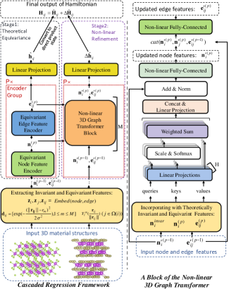
Figure 1: Left part: overview of the two-stage regression framework for Hamiltonian prediction, with the first stage extracting equivariant features and making baseline predictions, and the second stage enhancing accuracy via advanced non-linear networks. The first-stage network aids the second-stage network in learning SO(3)-equivariance, and the second-stage network compensates for the expressiveness capability of first-stage network. Right part: The internal architecture of the non-linear 3D graph Transformer network, the core module of the proposed method.

4 Method

As shown in Fig. 1, to alleviate the covariance-expressiveness dilemma analyzed in previous sections, we propose a novel two-stage cascaded regression framework effectively hybridizing a theoretically guaranteed SO(3)-equivariant network in the first stage, with a highly expressive non-linear network in the second stage from both representation level as well as the regression target level for Hamiltonian prediction in crystalline material research. The network from the first stage provides essential support to the second stage in mastering SO(3)-equivariance, whereas the network in the second stage enriches the expressiveness capabilities of the whole framework. The combination of these two stages not only enhances expressiveness but also ensures robust covariance to reference frames, bringing accurate predictions for Hamiltonians despite coordinate transformations.

4.1 Initial Features

In our framework, the initial feature for the $i(1\leq i\leq N)$ th node is its node embedding, denoted as $\mathbf{z}_{i}$, a coordinate-independent SO(3)-invariant semantic embedding that marks its element type. Given the locality of the Hamiltonian (Li et al., 2022), each atom $j$ in the local set $\Omega(i)$ within the cutoff radius of an atom $i$ form an edge with $i$. From each edge, a Hamiltonian is defined. The initial features for edge $(i,j)$ include both SO(3)-invariant encodings and SO(3)-equivariant encodings. The former includes edge embeddings $\mathbf{z}_{ij}$ marking the types of interacting atom pairs, as well as the distance features $\mathbf{d}_{ij}$ in the form of Gaussian functions (Li et al., 2022); the latter is spherical harmonics (Schrödinger, 1926), denoted as $Y_{l}^{m}(\frac{\mathbf{r}_{ij}}{||\mathbf{r}_{ij}||})$, where $\frac{\mathbf{r}_{ij}}{||\mathbf{r}_{ij}||}$ describes the relative orientation between two atoms. Worth noting, a node and itself also possess a Hamiltonian. In other words, $i\in\Omega(i)$ and $\mathbf{e}_{ii}$ also forms a valid edge. In this case, $Y_{l}^{m}(\frac{\mathbf{r}_{ij}}{||\mathbf{r}_{ij}||})$ cannot be used to calculate directional features and a vector filled with $0$ is used as a substitute. The above initial features are used to model the Hamiltonian which obey SO(3)-equivariance, additionally, these features also inherently fulfill translational invariance with respect to global coordinates, another natural attribute of Hamiltonians.

4.2 The First Regression Stage

In our framework, the primary role of the first regression stage is to extract theoretically SO(3)-equivariant node and edge representations, denoted as $\mathbf{n}^{(p)}_{i}$ and $\mathbf{e}^{(p)}_{ij}$ respectively for the $p$ th ($1\leq p\leq P$) encoder group, and regress baseline Hamiltonian predictions, denoted as $\hat{\mathbf{h}}_{ij}$ in the direct sum state and $\hat{\mathbf{H}}_{ij}$ in the direct product state for each pair $(i,j)$, establishing a firm foundation on SO(3)-equivariance in both feature level and the regression target level. We directly choose DeepHE3 as the first-stage network, for two main reasons. First, the node and edge feature encoders in DeepHE3 comprehensively incorporate SO(3)-equivariant tensor operators to aggregate and propagate structural patterns, enabling equivariant encoding of 3D structural patterns from both local level to larger range. Second, some advanced operations that highly depend on non-linear mappings, e.g. attention, are difficult to thoroughly perform their SOTA performance with the restrictions on non-linear activation functions imposed by theoretical equivariance in the first stage. Thus, we just take DeepHE3 as the first-stage network and focus on developing the second-stage network, where no restrictions on non-linear activation are imposed.

4.3 The Second Regression Stage

The second regression stage of our framework is designed to fully exploit non-linear mappings to enhance the expressive capability of the whole framework. For that purpose, as shown in the right part of Fig. 1, we propose a 3D graph Transformer which effectively models 3D atomic structures and predicts non-linear correction terms that complement the predictions from the first stage, achieving high-precision Hamiltonian prediction. Yet, one key problem to solve lies that, non-linear projections might sacrifice the guarantee on theoretical SO(3)-equivariance of the regression framework, forcing the second-stage network to implicitly capture equivariance through learning from the data. Thus, we must address the difficulty of learning equivariance of Hamiltonians as discussed in Section 3. Our second-stage network adeptly resolves this issue, simultaneously capturing equivariance and enhancing expressive capabilities. This is primarily attributed to three pivotal mechanisms we design.

First, in the second regression stage, the prediction target is not the entire Hamiltonian but a correction term $\Delta\hat{\mathbf{H}}_{ij}$, relative to the first stage’s output, i.e. the initial Hamiltonian estimate $\hat{\mathbf{H}}_{ij}$. The sum of these two stages’ outputs forms the final prediction of the Hamiltonian: $\mathbf{H}_{ij}=\hat{\mathbf{H}}_{ij}+\Delta\hat{\mathbf{H}}_{ij}$. Given that the predicted results of $\hat{\mathbf{H}}_{ij}$ are theoretically SO(3)-equivariant and approximately reasonable, the range of variations for the correction term $\Delta\hat{\mathbf{H}}_{ij}$, becomes smaller compared to $\hat{\mathbf{H}}_{ij}$. This reduces the complexity of the output space for the second stage and enhances the feasibility on implicitly capturing SO(3)-equivariance through data-driven learning for non-linear modules.

Second, the theoretically covariant features, including both SO(3)-equivariant and SO(3)-invariant features, are integrated into the input features of each Transformer block in the second stage to aid it in capturing equivariance, as shown in Eq. (1):

$$\begin{split}\mathbf{\widetilde{n}}^{\prime(p)}_{i}&=\mathbf{n}^{\prime(p-1)}_{i}+\alpha\mathbf{n}^{(p)}_{i}+\beta\mathbf{n}^{invar}_{i}\\ \mathbf{\widetilde{e}}^{\prime(p)}_{ij}&=\mathbf{e}^{\prime(p-1)}_{ij}+\lambda\mathbf{e}^{(p)}_{ij}\end{split}$$ (1)

where $\alpha$, $\beta$ and $\lambda$ are hyper-parameters, $\mathbf{n}^{\prime(p-1)}_{i}$ and $\mathbf{e}^{\prime(p-1)}_{ij}$ denote the outputs of the Transformer at the $p-1$ ${th}$ encoder group, $\mathbf{\widetilde{n}}^{\prime(p)}_{i}$ and $\mathbf{\widetilde{e}}^{\prime(p)}_{ij}$ respectively serve as the input node and edge features for the subsequent modules of the Transformer at the $p$ ${th}$ encoder group, $\mathbf{n}^{(p)}_{i}$ and $\mathbf{e}^{(p)}_{ij}$ are the SO(3)-equivariant node and edge features, respectively, from the corresponding encoder group of the first-stage network. Besides SO(3)-equivariant features, since as demonstrated by literature (Wang et al., 2018; Zhang et al., 2019; Zhang & Jiang, 2023), SO(3)-invariant features also facilitate the learning of SO(3)-equivariance, we also develop a SO(3)-invariant node feature, i.e., $\mathbf{n}^{invar}_{i}$, aggregated from multiple SO(3)-invariant features, such as node embeddings $\mathbf{z}_{i}$, edge embeddings $\mathbf{z}_{ij}$, distance features $\mathbf{d}_{ij}$, and triplet angle feature $\theta_{ijk}$ formed by node $i$ as well as two of its local atoms $j$ and $k$, in the way like:

$$\mathbf{n}^{invar}_{i}=\sum_{(j,k)\in\Omega(i)}FC(cat(\mathbf{z}_{i},\mathbf{z}_{j},\mathbf{z}_{k},\mathbf{d}_{ij},\mathbf{d}_{ik},\mathbf{c}_{ijk})))$$ (2)

where $cat(\cdot)$ is the concatenation operator, $FC(\cdot)$ denotes fully-connected layers with non-linear activations, $\mathbf{c}_{ijk}=[\cos(\theta_{ijk}),\cos(\theta_{ijk}),...]$ is a vector extended by duplication, which serves to amplify the angle features for $FC(\cdot)$. To reduce the quadratic complexity, i.e., $O(|\Omega(i)|^{2})$ when sampling $(j,k)\in\Omega(i)$, we arrange the set $\Omega(i)$ as an array and only extract adjacent element pairs as tuples $(j,k)$, lowing down the sampling complexity to $O(|\Omega(i)|)$ to efficiently compute $\mathbf{n}^{invar}_{i}$. In Eq. (1), $\mathbf{n}^{invar}_{i}$ is directly merged into node features, and since node features are then merged into edge features in the subsequent modules, it also enhances the learning of edge features. With the help of theoretically covariant features, the second-stage network, even a non-linear one, can better capture the SO(3)-equivariant properties inherent in the Hamiltonian.

Third, as the core of the Transformer, we design a multi-head attention mechanism to learn node and edge representations of the 3D atomic system. The capability to dynamically focus on related geometric features enables robust adaptability to diverse geometric conditions, from structural variants to coordinate transformations. Specifically, the attention mechanism firstly learns dynamic weights, i.e. $\alpha^{(p)}_{ij}$ for the edge $(i,j)$ at the $p$ th encoder group, based on the interactive relationship between the current atom $i$ and its local atoms $j\in\Omega(i)$, as shown in Eq. (LABEL:eq:bs1):

$$\begin{split}&\textbf{q}^{h(p)}_{ij}=\textbf{W}^{h}_{q}\cdot cat(\mathbf{\widetilde{n}}^{\prime(p)}_{i},\mathbf{\widetilde{e}}^{\prime(p)}_{ij}),\\ &\textbf{k}^{h(p)}_{ij}=\textbf{W}^{h}_{k}\cdot cat(\mathbf{\widetilde{n}}^{\prime(p)}_{j},\mathbf{\widetilde{e}}^{\prime(p)}_{ij})\\ &\alpha^{(p)}_{ij}=softmax(\frac{(\textbf{q}^{h(p)}_{ij})^{T}\cdot\textbf{k}^{h(p)}_{ij}}{\sqrt{d_{h}}})\end{split}$$ (3)

where $h(1\leq h\leq H)$ is the head index, $d_{h}$ is the dimension of features, $\textbf{W}^{h}_{q}$ and $\textbf{W}^{h}_{k}$ are parameter matrices to calculate queries and keys, i.e., $\textbf{q}^{h(p)}_{ij}$ and $\textbf{k}^{h(p)}_{ij}$, respectively. Here the scale factor $\sqrt{d_{h}}$ in the denominator is used to prevent $softmax(\cdot)$ from gradient saturation, and the multiple heads aim at enchaining the model capacity. Based on $\alpha^{(p)}_{ij}$, the node features are updated flexibly through the structural information embedded in its local sets, as shown in Eq. (LABEL:eq:bs2):

$$\begin{split}&\mathbf{v}^{h(p)}_{i}=\sum_{j\in\Omega(i)}\alpha^{(p)}_{ij}\cdot(\textbf{W}^{h}_{v}\cdot cat(\mathbf{\widetilde{n}}^{\prime(p)}_{j},\mathbf{\widetilde{e}}^{\prime(p)}_{ij})),\\ &\mathbf{n}^{\prime(p)}_{i}=FC(LN(\textbf{W}_{o}\cdot cat(\mathbf{v}^{1(p)}_{i},...,\mathbf{v}^{H(p)}_{i})+\mathbf{n}^{\prime(p-1)}_{i}))\end{split}$$ (4)

where $LN(\cdot)$ is the layer normalization operator, $FC(\cdot)$ denotes fully-connected layers with non-linear activations. Based on $\mathbf{n}^{\prime(p)}_{i}$, the edge representations are updated as:

$$\mathbf{e}^{\prime(p)}_{ij}=FC(cat(\mathbf{n}^{\prime(p)}_{i},\mathbf{n}^{\prime(p)}_{j},\mathbf{e}^{\prime(p-1)}_{ij})))$$ (5)

when repeatedly stacking operations in Eq. (LABEL:eq:bs2) and (5) in an alternate manner, local patterns can incrementally spread to a larger scale through the neighbors of neighboring atoms. Nevertheless, given the Hamiltonian’s locality, there’s typically no need for information transfer over very long distances. Finally, the correction term outputted by the second stage is regressed from the edge features $\mathbf{e}^{\prime(P)}_{ij}$ encoded by the last encoder group, in the way like:

$$\Delta\hat{\mathbf{H}}_{ij}=DStoDP(\Delta\hat{\mathbf{h}}_{ij})=DStoDP(FC(\mathbf{e}^{\prime(P)}_{ij}))$$ (6)

where $DStoDP(\cdot)$ is the conversion operation from the vector-formed direct sum state to the matrix-formed direct product state, which is more commonly used in the down-stream computational tasks based on Hamiltonians.

4.4 Training

Considering that networks from the two stages employ fundamentally different operators, training them simultaneously in a joint manner may pose optimization difficulties. Therefore, we optimize them separately. In the first stage, parameters of the first-stage network are optimized by minimizing $MSE(\mathbf{H}^{*}_{ij}-\hat{\mathbf{H}}_{ij})$, while in the second stage, parameters of the second-stage network are optimized by minimizing $MSE((\mathbf{H}^{*}_{ij}-\hat{\mathbf{H}}_{ij})-\Delta\hat{\mathbf{H}}_{ij})$. To avoid interference, the networks of the two stages use independent node and edge embeddings; moreover, during the training of the second-stage network, gradients are not propagated back to the first-stage network. To facilitate the implicit learning of SO(3)-equivariance for non-linear modules, rigid rotational data augmentation on the training samples is introduced. Adam is used for optimization.

5 Discussion on Time Complexity

The time complexity for both of the first-stage and the second-stage networks are $\mathcal{O}(BNE)$, where $B$ is the number of their basic blocks, $N$ is the total number of atoms in a system, $E$ is the average number of atoms within the cutoff radius of a given atom. Due to the locality of the Hamiltonian, for a given class of atomic systems, $E$ is roughly a constant and does not significantly increase with the growth of $N$. Therefore, for big atomic systems with very large $N$, $E\ll N$, and similarly, $B\ll N$. In this case, the time complexity of our framework tends towards $\mathcal{O}(N)$. In contrast, for traditional DFT method (Kohn & Sham, 1965), which requires $T$ rounds of iterative decomposition of $N\times N$ matrices, the time complexity is $O(TN^{3})$. As $N$ increases, the cubic complexity of $N$ results in significant computational overhead, and to achieve self-consistency, $T$ is usually very large, exacerbating the computational burden, leading to the difficulties for simulations of large atomic systems within an acceptable time frame. On the contrary, our framework offers an efficient pathway for simulating large atomic systems with linear time complexity of $N$ and without the need for $T$ rounds of iterations.

6 Experiments

6.1 Experimental Conditions

We conduct experiments on six crystalline material databases, including Monolayer Graphene (abbreviated as MG), Monolayer MoS2 (MM), Bilayer Graphene (BG), Bilayer Bismuthene (BB), Bilayer Bi2Te3 (BT), and Bilayer Bi2Se3 (BS), which are released by the DeepH series (Li et al., 2022; Gong et al., 2023) with CC BY 4.0 license. The training, validation, and test sets as well as the data pre-processing protocols we use are exactly the same as DeepHE3. A concise overview of these databases is presented in Table 1. For more details, please refer to the original papers of these databases. These databases are diverse and representative, as they cover materials with strong chemical bonds within individual layers and weak vdW interactions between layers; and include varied degrees of SOC, featuring both strong SOC samples like BT, BB and BS, and others with weak SOC. Predicting the Hamiltonian accurately for these materials poses a significant challenge due to the presence of structural deformations caused by thermal motions and inter-layer twists, as shown in Fig. 2. Worth noting, the twisted materials have become a research hotspot due to their potentials for new electrical and quantum topological properties (Cao et al., 2018). During the twist transformations, the relative rotation between atoms and the coordinate system brings the corresponding SO(3)-equivariant effects; meanwhile, the change in orientations between two layers of atoms causes variations in vdW interactions. These combined effects present a challenge to both of the equivariance and expressiveness capabilities of the regressor. In our experiments, the twisted subsets are even difficult as there are no such samples in the training set.

To ensure the reproducibility, we follow DeepHE3 to use a fixed random seed, i.e., $42$, for all procedures involving randomness, such as parameter initialization, data loader, as well as the rigid rotational augmentation introduced during training. Our experiments are conducted on an internal cluster of Tesla A100 servers where $16$ cards are used, each with 80 GiB of GPU memory. Details on hyper-parameter selection are attached in the appendix A.

As ablation studies, we set up several groups of experiments, each of which removes a key mechanism of our method from training and testing. Specifically, $Ours^{-cas}$ removes the cascaded regression mechanism, by making predictions of the complete Hamiltonian, rather than its corrective term, directly from the regression head of the second stage; $Ours^{-cov}$ removes the mechanism of integrating theoretically covariant features into the input layers of Transformer blocks in the second stage; $Ours^{-att}$ removes the attention mechanism from the Transformer and replace it by mixing neighboring features with stationary weights similar to DeepHE3; we also report the results predicted individually by the first-stage network, i.e., DeepHE3, reproduced with its one-click reproduction scripts in the latest resources, from which the reproduced results are slightly better than those reported in their original paper (Gong et al., 2023). Experimental results of our complete method ($Ours$) as well as the ablation terms on the six material databases are presented in Table 2 and 3, where the former details the results for monolayer structures, and the latter focuses on bilayer structures. For comparison, In Table 2 and 3, the Mean Absolute Error (MAE) metric is used as the accuracy metric. Besides the classical MAE metric, denoted as $MAE_{all}$, which measures the average error among all testing samples, the MAE on the most challenging sample with worst accuracy from each database is also a crucial metric. We record it as $MAE_{cha}$, to distinguish it from $MAE_{all}$. To offset the randomness of experiments, we conduct independent experiments for $10$ times repeatedly and report $MAE_{all}$ and $MAE_{cha}$, averaged across these $10$ experiments. Additionally, we report the standard deviation ( $\pm\sigma$), a bar measuring the statistical fluctuation of the experimental results in Table 2 and 3. In addition to taking the Hamiltonian of each edge as a whole for accuracy statistics like in Table 2 and 3, since the Hamiltonian matrix in the direct product state is constituted by several basic blocks based on the angular momentum of interacting orbitals, fine-grained accuracy statistics on these blocks are also conducted, as shown in the appendix B.

Table 1: Brief statistics of experimental databases on the sizes of training, validation, and testing sets including both non-twisted samples (NT) and twisted samples (T), as well as the dimensions of the Hamiltonians in the direct sum state for each atom pair.

	MG	MM	BG	BB	BT	BS
Train (NT)	270	300	180	231	204	231
Val (NT)	90	100	60	113	38	113
Test (NT)	90	100	60	113	12	113
Test (T)	-	-	9	4	2	2
$\textnormal{Dim}(\textnormal{{h}}_{ij})$	169	361	169	2888

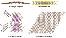
Figure 2: Visualization of challenging testing samples, which exhibit structural deformations caused by thermal motions and inter-layer twists, calling for strong capabilities on expressiveness and SO(3)-equivariance of a regression model.

Table 2: Comparison of experimental results on monolayer material databases. Both the mean and standard deviation of $MAE_{all}$ as well as $MAE_{cha}$ (/meV) from $10$ independent repeated experiments are provided.

Dataset	Method	$MAE_{all}$	$MAE_{cha}$
MG	DeepHE3	0.251 $\pm$ 0.002	0.357 $\pm$ 0.002
	$Ours^{-cas}$	0.774 $\pm$ 0.005	0.880 $\pm$ 0.006
	$Ours^{-cov}$	0.243 $\pm$ 0.001	0.328 $\pm$ 0.002
	$Ours^{-att}$	0.221 $\pm$ 0.002	0.297 $\pm$ 0.001
	$Ours$	0.176 $\pm$ 0.001	0.267 $\pm$ 0.001
MM	DeepHE3	0.406 $\pm$ 0.002	0.574 $\pm$ 0.003
	$Ours^{-cas}$	0.927 $\pm$ 0.004	0.958 $\pm$ 0.003
	$Ours^{-cov}$	0.384 $\pm$ 0.002	0.414 $\pm$ 0.002
	$Ours^{-att}$	0.319 $\pm$ 0.001	0.366 $\pm$ 0.002
	$Ours$	0.233 $\pm$ 0.001	0.293 $\pm$ 0.002

Table 3: Comparison of experimental results on bilayer material databases and the twisted subsets, where the superscripts $nt$ and $t$ denote the non-twisted and twisted testing samples, respectively.

Dataset	Method	$MAE_{all}$	$MAE_{cha}$
BGnt	DeepHE3	0.389 $\pm$ 0.002	0.453 $\pm$ 0.003
	$Ours^{-cas}$	0.854 $\pm$ 0.003	0.920 $\pm$ 0.004
	$Ours^{-cov}$	0.365 $\pm$ 0.002	0.427 $\pm$ 0.002
	$Ours^{-att}$	0.348 $\pm$ 0.001	0.419 $\pm$ 0.003
	$Ours$	0.287 $\pm$ 0.002	0.362 $\pm$ 0.002
BBnt	DeepHE3	0.274 $\pm$ 0.003	0.304 $\pm$ 0.002
	$Ours^{-cas}$	0.802 $\pm$ 0.003	0.873 $\pm$ 0.004
	$Ours^{-cov}$	0.249 $\pm$ 0.004	0.281 $\pm$ 0.004
	$Ours^{-att}$	0.243 $\pm$ 0.001	1.326 $\pm$ 0.003
	$Ours$	0.172 $\pm$ 0.001	0.198 $\pm$ 0.002
BTnt	DeepHE3	0.447 $\pm$ 0.001	0.480 $\pm$ 0.002
	$Ours^{-cas}$	0.930 $\pm$ 0.004	1.026 $\pm$ 0.004
	$Ours^{-cov}$	0.439 $\pm$ 0.001	0.466 $\pm$ 0.003
	$Ours^{-att}$	0.385 $\pm$ 0.001	0.414 $\pm$ 0.002
	$Ours$	0.294 $\pm$ 0.002	0.321 $\pm$ 0.002
BSnt	DeepHE3	0.397 $\pm$0.003	0.424 $\pm$0.001
	$Ours^{-cas}$	0.898 $\pm$ 0.005	0.960 $\pm$ 0.005
	$Ours^{-cov}$	0.392 $\pm$ 0.002	0.401 $\pm$ 0.001
	$Ours^{-att}$	0.348 $\pm$ 0.002	0.375 $\pm$ 0.003
	$Ours$	0.282 $\pm$ 0.002	0.308 $\pm$ 0.002
BGt	DeepHE3	0.264 $\pm$ 0.003	0.429 $\pm$ 0.003
	$Ours^{-cas}$	0.801 $\pm$ 0.005	0.863 $\pm$ 0.004
	$Ours^{-cov}$	0.312 $\pm$ 0.003	0.441 $\pm$ 0.004
	$Ours^{-att}$	0.278 $\pm$ 0.002	0.428 $\pm$ 0.002
	$Ours$	0.227 $\pm$ 0.002	0.403 $\pm$ 0.001
BBt	DeepHE3	0.468 $\pm$ 0.003	0.602 $\pm$0.004
	$Ours^{-cas}$	1.213 $\pm$ 0.004	1.569 $\pm$ 0.005
	$Ours^{-cov}$	0.530 $\pm$ 0.004	0.697 $\pm$ 0.004
	$Ours^{-att}$	0.504 $\pm$ 0.004	0.669 $\pm$ 0.005
	$Ours$	0.438 $\pm$0.003	0.578 $\pm$0.002
BTt	DeepHE3	0.831 $\pm$ 0.003	0.850 $\pm$ 0.003
	$Ours^{-cas}$	1.892 $\pm$ 0.003	1.937 $\pm$ 0.004
	$Ours^{-cov}$	0.928 $\pm$ 0.004	0.943 $\pm$ 0.004
	$Ours^{-att}$	0.837 $\pm$ 0.003	0.846 $\pm$ 0.003
	$Ours$	0.774 $\pm$ 0.002	0.794 $\pm$ 0.003
BSt	DeepHE3	0.370 $\pm$ 0.001	0.390 $\pm$ 0.002
	$Ours^{-cas}$	1.569 $\pm$ 0.003	1.892 $\pm$ 0.005
	$Ours^{-cov}$	0.415 $\pm$ 0.003	0.456 $\pm$ 0.003
	$Ours^{-att}$	0.392 $\pm$ 0.002	0.421 $\pm$ 0.002
	$Ours$	0.336 $\pm$ 0.001	0.365 $\pm$ 0.002

6.2 Experimental Results and Analysis

From Table 2 and 3, we could observe that our method significantly outperforms DeepHE3 on all of the experimental databases. Specifically, on MG, MM, BG^nt, BB^nt, BT^nt, BS^nt, BG^t, BB^t, BT^t and BS^t, we respectively lower down $MAE_{all}$ by a relative ratio of $29.88\%$, $42.61\%$, $26.22\%$, $37.23\%$, $34.23\%$, $28.97\%$, $14.02\%$, $6.41\%$, $6.86\%$, and $9.19\%$, respectively, and lower down $MAE_{cha}$ by $25.21\%$, $48.95\%$, $20.09\%$, $34.87\%$, $33.13\%$, $27.36\%$, $6.06\%$, $3.99\%$, $6.59\%$, and $6.41\%$, correspondingly, compared to DeepHE3. From the block-level experimental results presented in appendix B, we further discern that our method outperforms DeepHE3 in the vast majority of blocks of Hamiltonian matrices, especially on those blocks where DeepHE3 performs the worst. These results indicate that our method excels in accuracy, both on average and for the most challenging samples and blocks. The key to this enhanced performance lies in addressing the limitations inherent in DeepHE3. While DeepHE3 ensures theoretical symmetry, it restricts the use of non-linear activation functions, leading to a constrained expressive capability and a bottleneck in generalization performance. To overcome this, we evolve it into a two-stage regression framework incorporating a non-linear network, i.e. a 3D graph Transformer with good generalization potentials to the diverse geometric conditions, capturing the complexity of Hamiltonians via enhanced expressiveness capability. Particularly, the results on twisted samples demonstrate that, our method, despite the extensive use of non-linear operators, can still capture the symmetry properties of Hamiltonians and make covariant predictions under rotational operations. As shown in Table 1, the Hamiltonian of each atom pair is high-dimensional. In the presence of thermal motions and bilayer twists, the Hamiltonian varies across a vast label space, posing a significant challenge for non-linear networks in a lack of theoretical guarantee on covariance to predict the Hamiltonians accurately, especially for twisted samples with strong rotations. Yet, we conquer these difficulties and successfully enable the non-linear network to perform effectively, and the reasons for this success can be inferred from the ablation studies. By comparing the results of the three ablation terms, i.e., $Ours^{-cas}$, $Ours^{-cov}$, $Ours^{-att}$, with our complete method ($Ours$), we could observe that the cascaded regression mechanism, the covariant feature integration mechanism, as well the multi-head attention mechanism, all contribute significantly to the performance of our method. The cascaded regression mechanism, by reducing the output space of the non-linear network, eases the difficulties on non-linear regression of Hamiltonians with SO(3)-equivariance; the covariant feature integration mechanism, through leveraging theoretically covariant features from DeepHE3 and geometric knowledge, successfully assists the non-linear network in learning SO(3)-equivariance; the multi-head attention mechanism, by assigning dynamic weights when fusing features, adapts to the wide variation range of geometric conditions, including both thermal deformations and twists. Under the novel combination of these mechanisms, the first-stage network, i.e., DeepHE3 and the second-stage, namely the non-linear Transformer, complement each other effectively, making our framework possess both excellent expressiveness capability and covariance performance to achieve good results.

Among current deep learning studies on Hamiltonians modeling, the DeepH series have conducted comprehensive experiments on various types of crystalline materials, proving SOTA performance. The paper of DeepHE3 has demonstrated it to surpass DeepH in accuracy by developing covariant mechanisms; and since our method further outperforms DeepHE3 through harmonizing covariance and expressiveness of neural networks, we may conclude that our work represents the new SOTA in the field of deep Hamiltonian regression on crystal material analysis.

Based on the experimental results, a limitation analysis of our method and the future work plan is given in appendix C.

7 Conclusion

In crystalline material research, deep learning for Hamiltonian regression requires adherence to covariance laws, facing a pivotal challenge to achieve SO(3)-equivariance without compromising network expressiveness, due to the restriction on non-linear functions to theoretically guarantee equivariance. To address this, we propose a two-stage cascaded regression framework, where the first stage employs a theoretically-informed covariant neural network for modeling the covariant properties of 3D atomic structures, yielding baseline Hamiltonians with series of covariant features assisting the subsequent stage on capturing SO(3)-equivariance. The second stage, leverages the proposed non-linear 3D graph Transformer network for fine-grained structural analysis of 3D atomic systems, refining the initial Hamiltonian predictions via enhanced network expressiveness. Such a combination allows for accurate, generalizable Hamiltonian predictions while upholding strong covariance against coordinate transformations. Our methodology demonstrates SOTA performance in Hamiltonian prediction, validated through six crystalline material databases.

Impact Statements

This paper presents work whose goal is to advance the field of machine learning and material research. It has no evident and direct negative impacts on society and ethics. A broader discussion on impacts is given in appendix D.

Appendix A Determination of Hyper-parameters

Regarding hyper-parameter selection, to ensure fairness in comparison, for the first-stage network (DeepHE3), we use the same hyper-parameters as those gathered in its latest open-source project. For the Transformer network we propose in the second regression stage, we conduct hyperparameter selection according to the $MAE_{all}$ performance on the validation sets. The hyperparameters to be searched include: the number of Transformer blocks ($M$) within one encoder group $p$ $(1\leq p\leq P)$, where $P$ is set as $3$ in advance to align with DeepHE3; the coefficients ($\alpha$,$\beta$,$\lambda$) for feature fusion in Eq. (LABEL:eq:bs1); the training batch size $W$; as well as the learning rare $\gamma$. They are searched from: $1\leq M\leq 6$, $\alpha,\beta,\lambda\in\{0.0,0.1,...,1.5\}$, $1\leq W\leq 3$, and $\gamma\in\{1*10^{-4},2*10^{-4},...,1*10^{-3}\}$. To select hyper-parameters efficiently, a coarse-to-fine grid search is conducted. In the search process, we select the minimum value for each hyper-parameter at which further increasing its value does not lead to a significant improvement ($p\_value<0.05$) on the validation sets. Their optimal values identified through this search are as follows: $M^{*}=4$, $\alpha^{*}=0.8$, $\beta^{*}=0.9$, $\lambda^{*}=0.4$, $W=1$, $\gamma^{*}=3*10^{-4}$. Notably, although our method is independently trained on the training set of each individual material database, to obtain a set of general hyper-parameters, the overall performance across the validation sets of different materials is considered to select hyper-parameters. After hyper-parameter selection, our method is retrained on each individual training set according to the optimal hyper-parameters until converge.

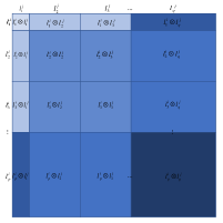
Figure 3: An illustration of the basic blocks constituting a Hamiltonian matrix $\mathbf{H}_{ij}$ in the direct product state. Assume the atom pair corresponding to the Hamiltonian matrix is $i$ and $j$, where atom $i$ corresponds to orbitals with angular momentum $l^{i}_{1},l^{i}_{2},\ldots,l^{i}_{p}$, and atom $j$ corresponds to orbitals with angular momentum $l^{j}_{1},l^{j}_{2},\ldots,l^{j}_{q}$. The interaction between each pair of orbitals forms a basic block.

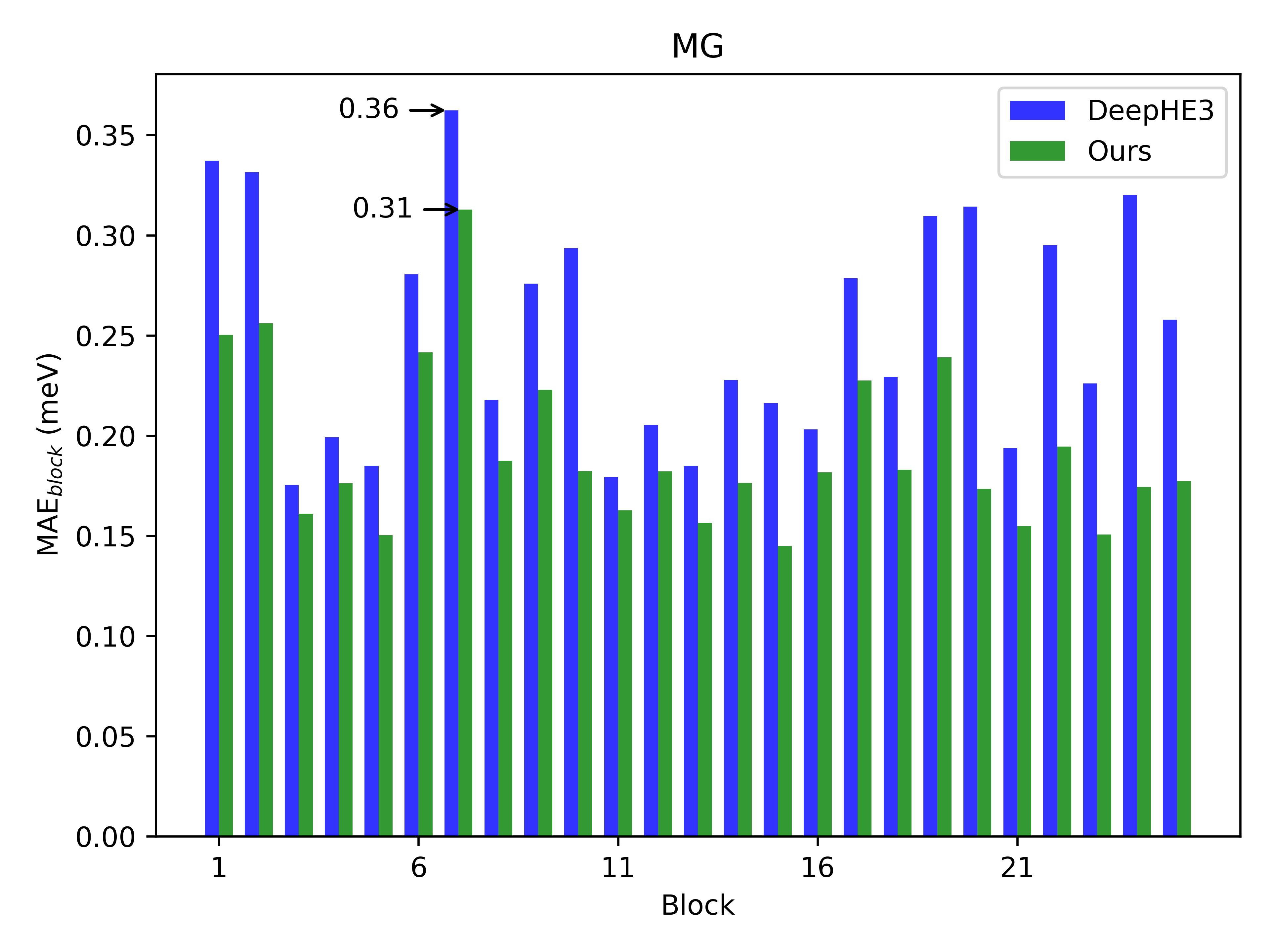
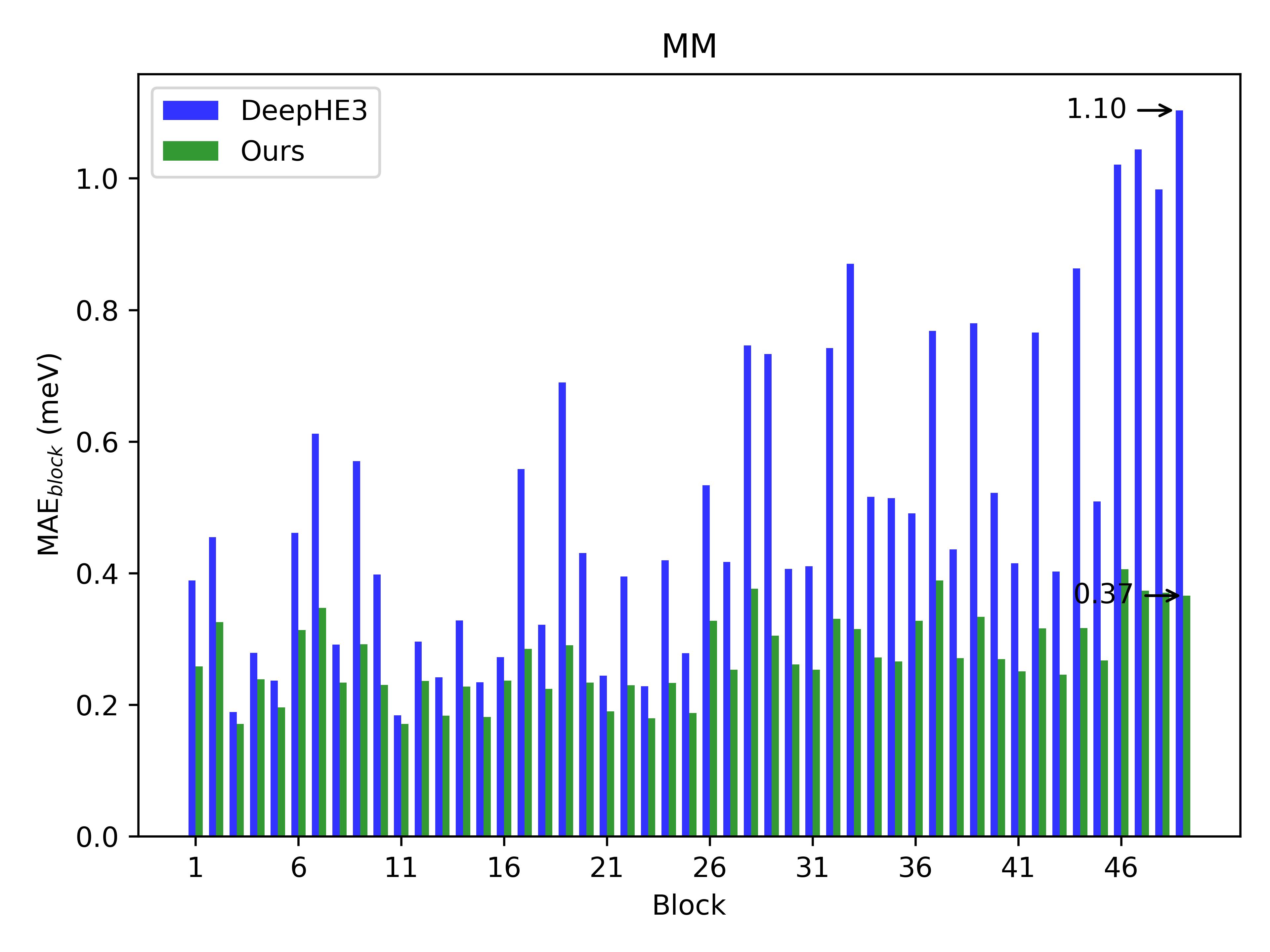
Figure 4: The MAE values (denoted as $MAE_{\text{block}}$) on various basic blocks of the Hamiltonian matrix in direct product state on the experimental monolayer material databases. The reported $MAE_{\text{block}}$ for each block are the mean from 10 independent repeated experiments.

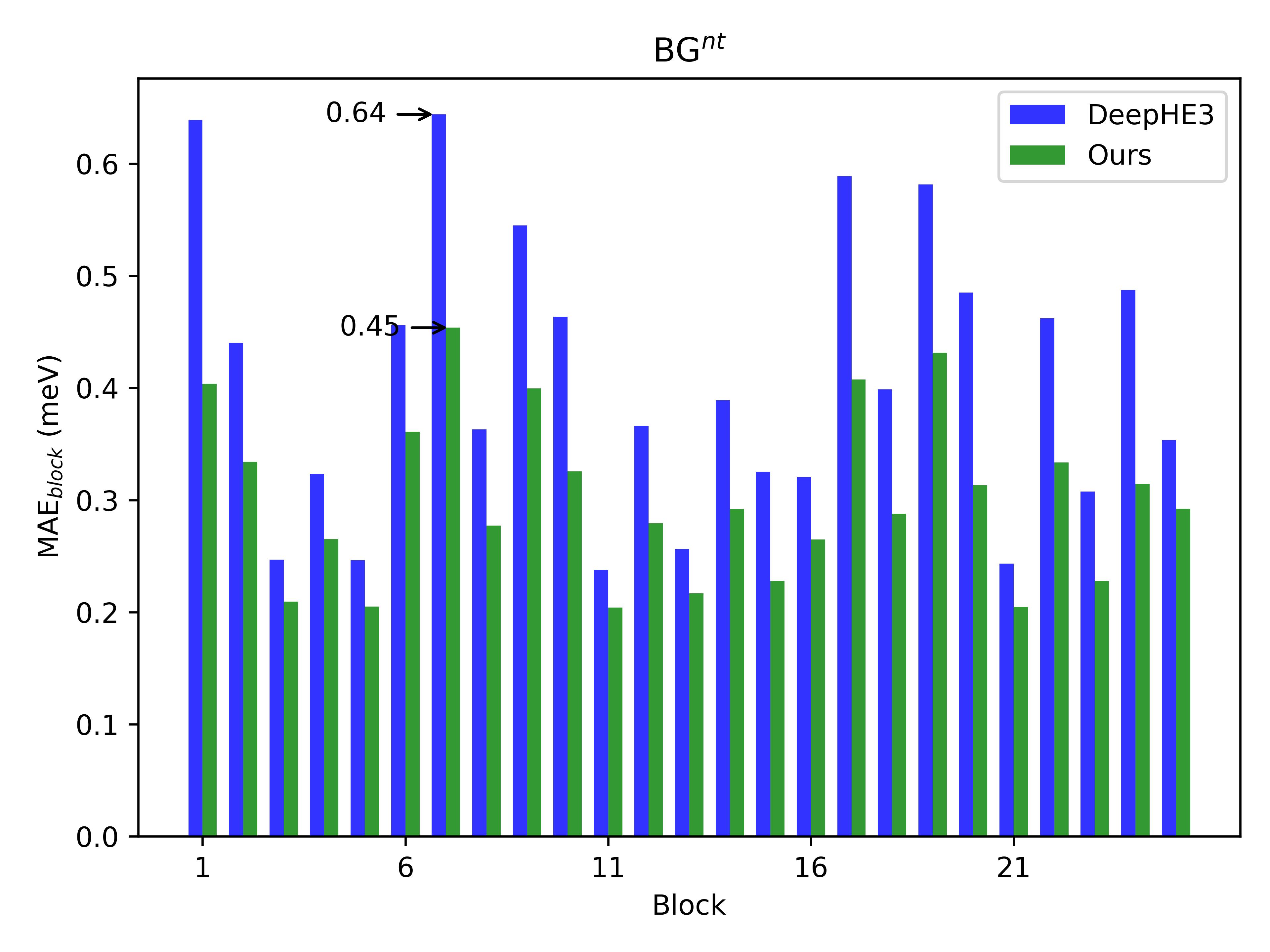
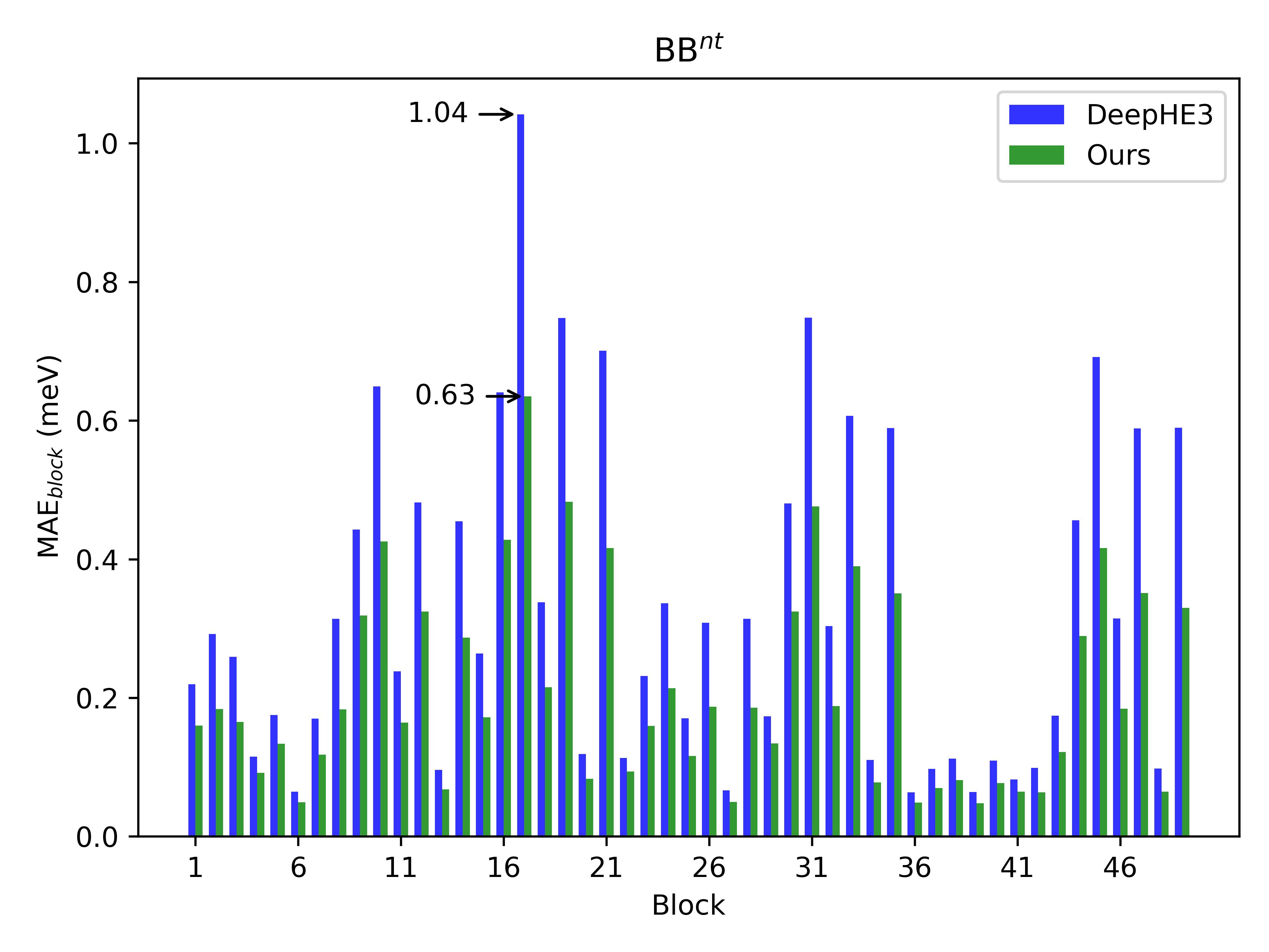
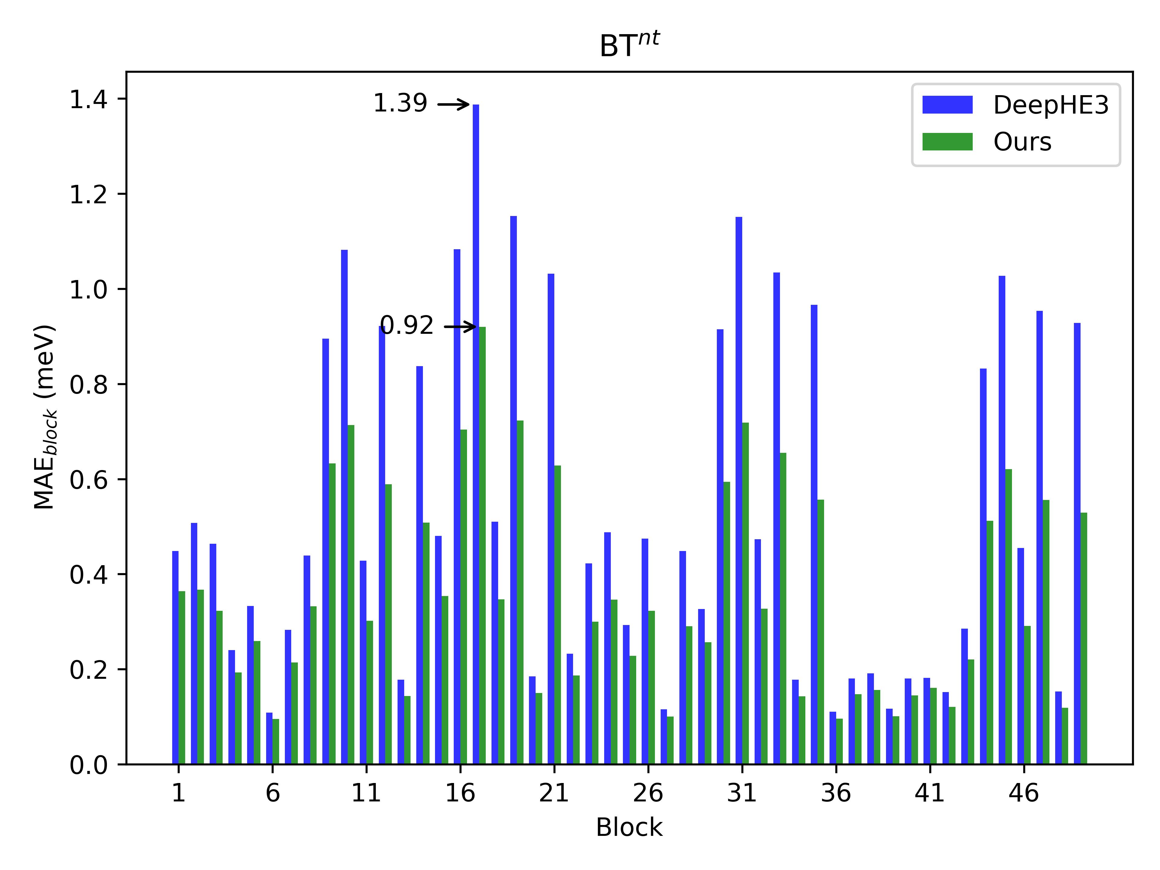
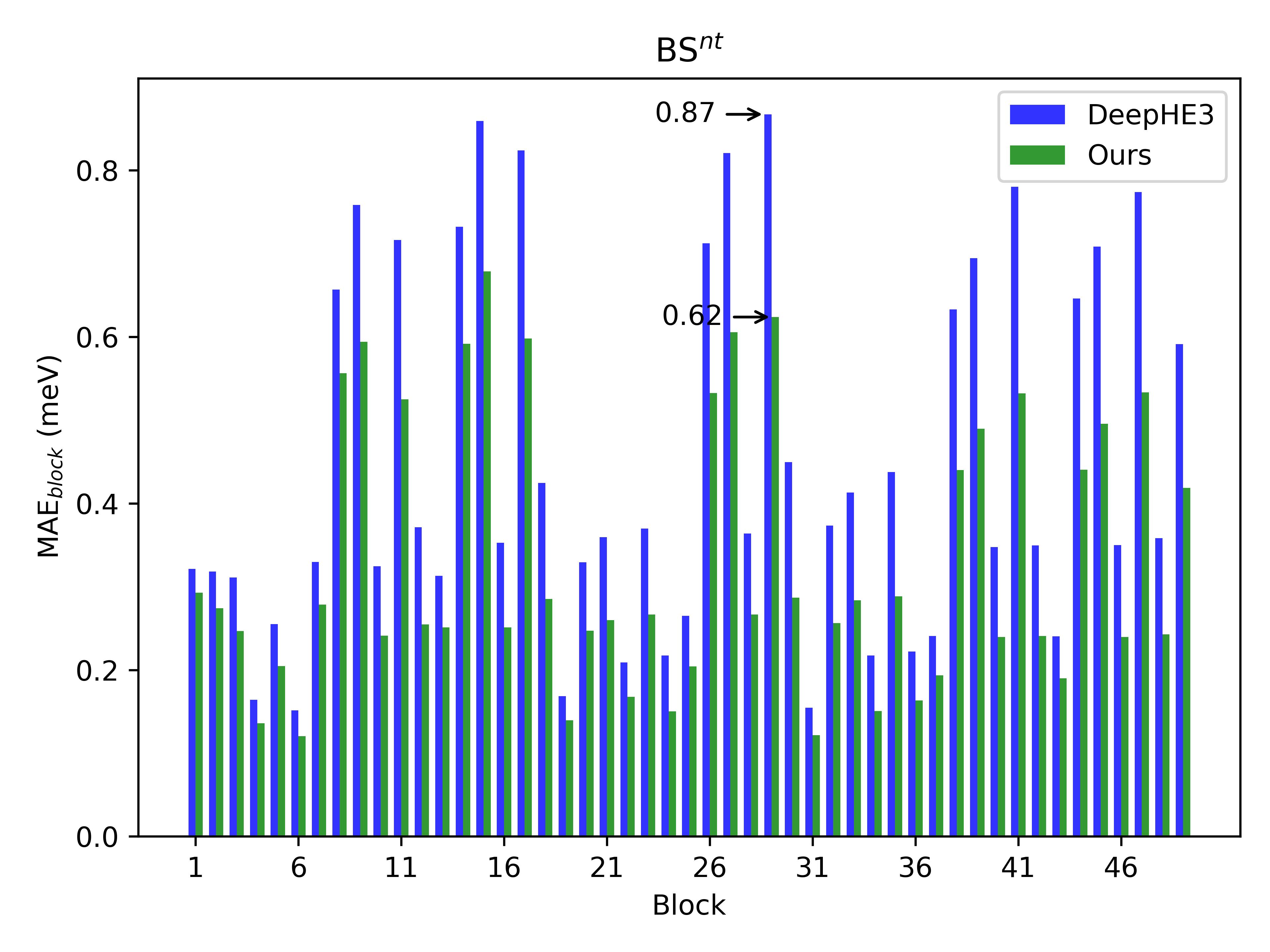
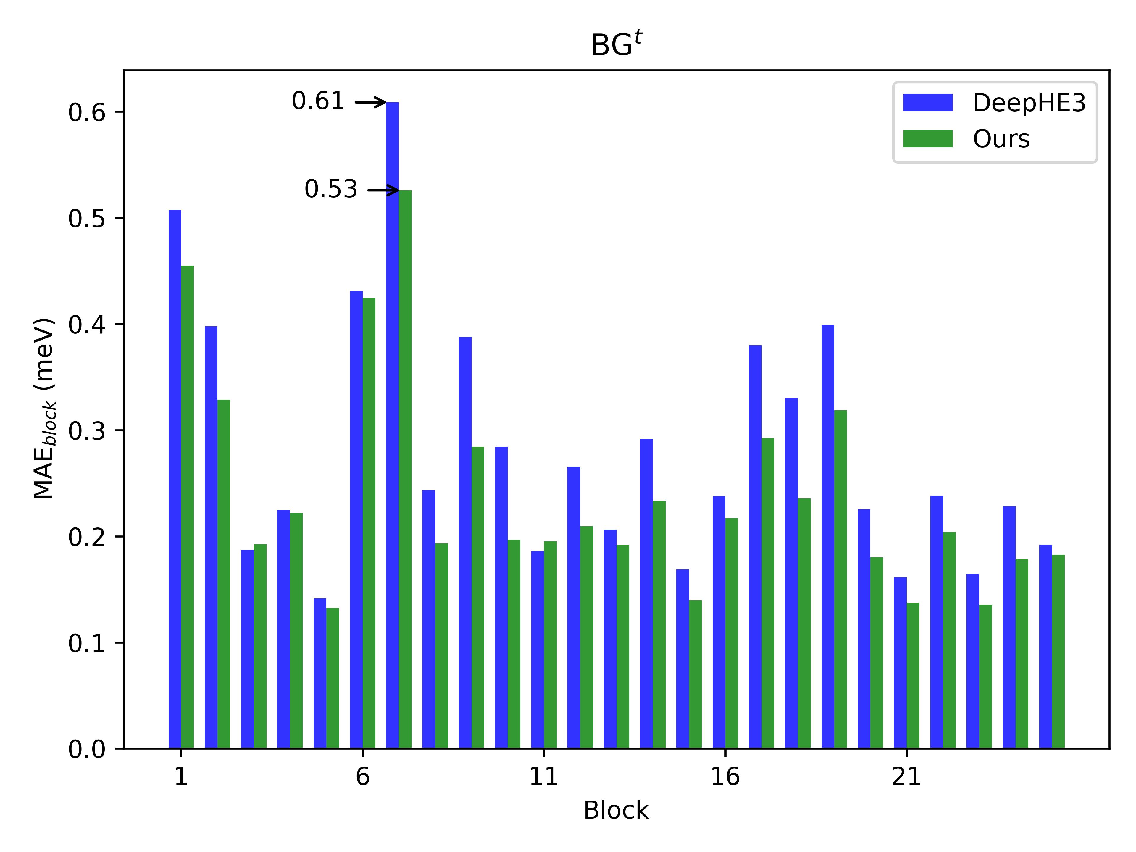
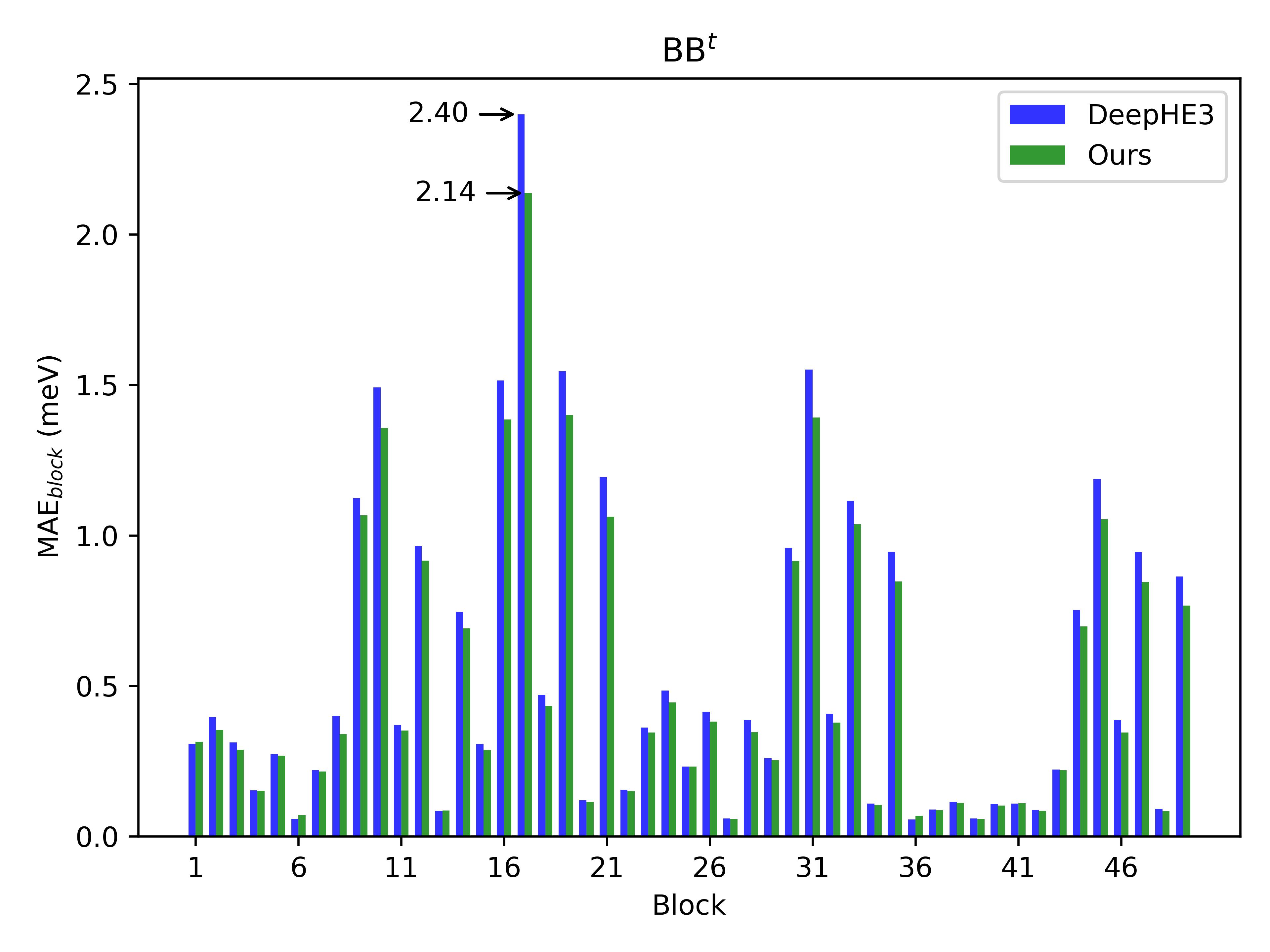
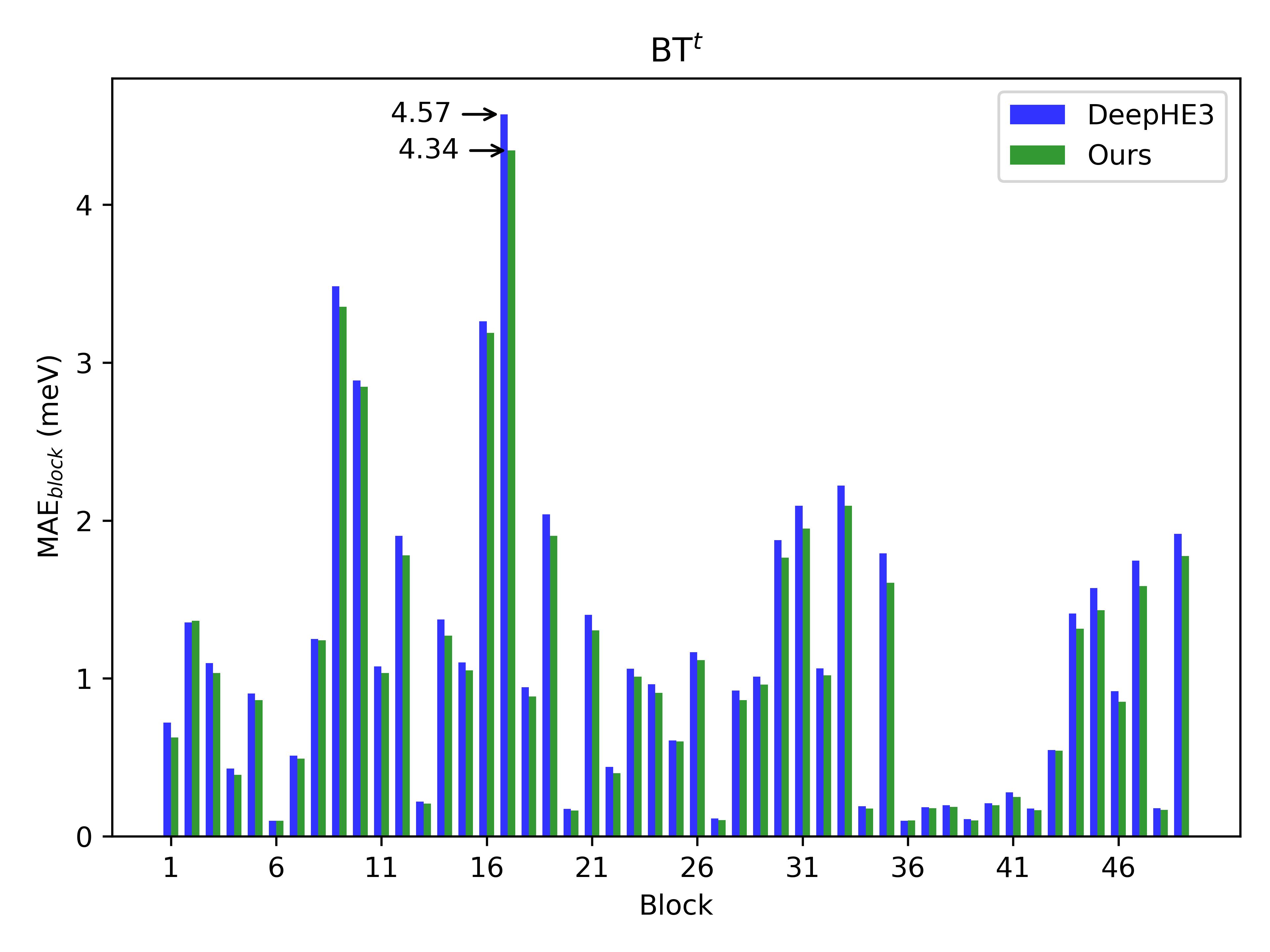
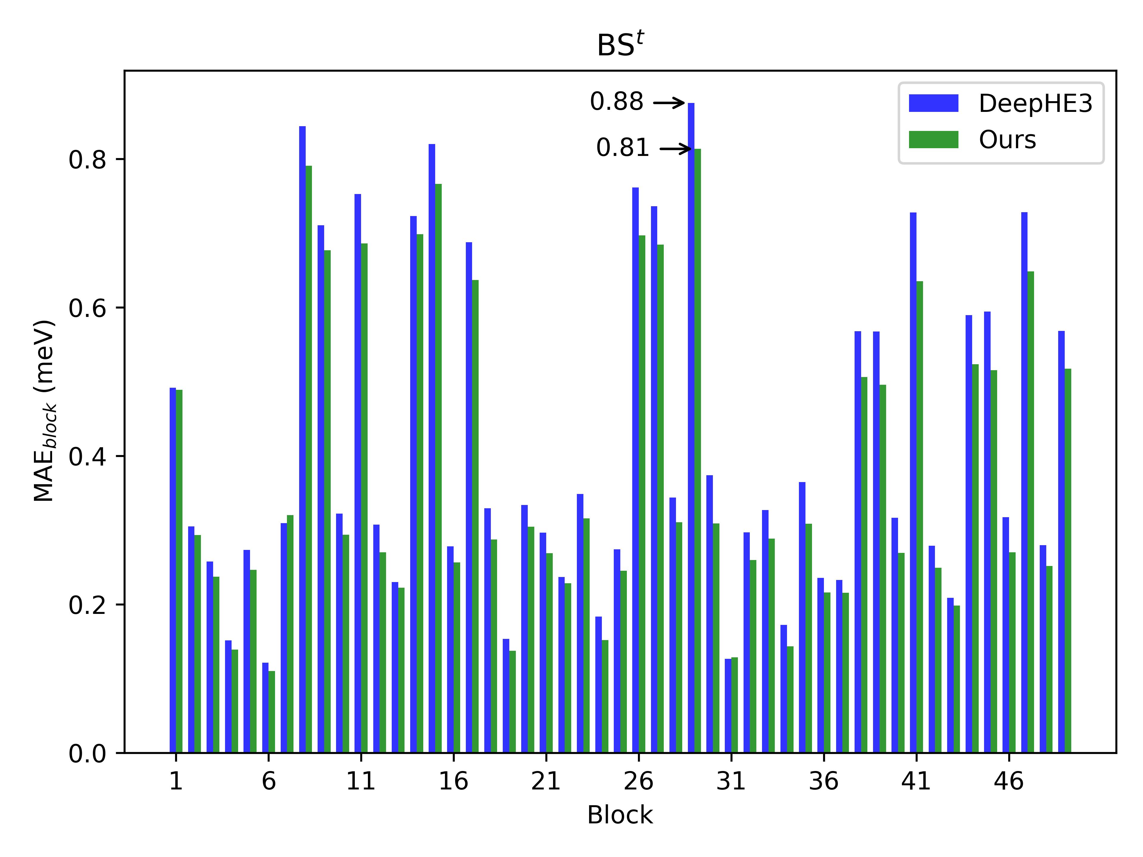
Figure 5: The MAE values (denoted as $MAE_{\text{block}}$) on various basic blocks of the Hamiltonian matrix in direct product state on the experimental bilayer material databases. The reported $MAE_{\text{block}}$ for each block are the mean from 10 independent repeated experiments.

Appendix B MAE Statistics on Basic Blocks of Hamiltonian Matrices

As shown in Fig. 3, the Hamiltonian matrix in the direct product state is constituted by several basic blocks based on the angular momentums of interacting orbitals. We here conduct fine-grained accuracy statistics on these basic blocks. MAE metrics (denoted as $MAE_{block}$) of our method ($Ours$) and DeepHE3 on different blocks of the Hamiltonian matrix of the six materials are presented in Fig. 4 and 5, where Fig. 4 illustrates the results on monolayer structures, and Fig. 5 is dedicated to bilayer structures. Combing the results on Fig. 4 and 5, we observe that we outperform DeepHE3 in the vast majority of basic blocks, especially in those where DeepHE3 performs the worst. Specifically, on the databases of MG, MM, BG^nt, BB^nt, BT^nt and BS^nt, BG^t, BB^t, BT^t, and BS^t, our method reduces the MAE of the Hamiltonian blocks where DeepHE3 performs the worst by $13.89\%$, $66.36\%$, $29.69\%$, $39.42\%$, $33.81\%$, $28.74\%$, $13.11\%$, $10.83\%$, $5.03\%$ and $7.95\%$, respectively. The significant accuracy improvements on the most challenging blocks are critical, as errors in these areas are most likely to cause precision bottlenecks of downstream computational physics tasks.

Appendix C Limitations and Future Works

From the experimental results presented in Fig. 3, we could observe that, although our method significantly outperforms DeepHE3, there still exists some improvement scopes on the challenging blocks of Hamiltonian matrices. The task of predicting the Hamiltonian calls for ultra-high precision and covariance performance at the sub-meV level. However, due to the high-dimensional and complex nature of the Hamiltonians, achieving such a level of accuracy consistently across all blocks is extremely challenging. To enhance and balance the performance across all blocks, especially for the challenging ones, our future work will focus on three main directions. First, we will explore dynamic loss functions for each Hamiltonian block to adjust learning strategies based on the fitting challenges and balance the fitting and generalization performance on different blocks. Second, we will employ ensemble learning methods to dynamically integrate models with complementary strengths in predicting different blocks. Third, we will explore advanced representation learning techniques, such as self-supervised pre-training methods, to promote the performance on challenging blocks.

Appendix D Broader Discussion on Impacts

In our efforts to accurately predict material Hamiltonians using machine learning techniques, we have observed the significant potential of this method in accelerating materials science development. We recognize that, although our research field has not shown direct negative social or ethical consequences, there are several important issues that require our vigilance and attention. Currently, while our models can provide accurate predictions, their decision-making processes often lack transparency. This limits our deep understanding of the learning outcomes and subsequently constrains our capacity to extract deeper insights from these predictions. Additionally, ensuring the correctness and impartiality of the models is paramount. It is essential to maintain the high quality and diversity of input data, apply reasonable model designs, and undertake continuous verification and revision. These steps are crucial to ensure the models’ accuracy and that the results are universally applicable.

References

- Batzner et al. (2022) Batzner, S., Musaelian, A., Sun, L., Geiger, M., Mailoa, J. P., Kornbluth, M., Molinari, N., Smidt, T. E., and Kozinsky, B. E (3)-equivariant graph neural networks for data-efficient and accurate interatomic potentials. Nature Communications, 13(1):2453, 2022.
- Cao et al. (2018) Cao, Y., Fatemi, V., Fang, S., Watanabe, K., Taniguchi, T., Kaxiras, E., and Jarillo-Herrero, P. Unconventional superconductivity in magic-angle graphene superlattices. Nature, 556(7699):43–50, 2018.
- Cohen & Welling (2017) Cohen, T. S. and Welling, M. Steerable cnns. In ICLR, 2017.
- Dieleman et al. (2016) Dieleman, S., Fauw, J. D., and Kavukcuoglu, K. Exploiting cyclic symmetry in convolutional neural networks. In ICML Workshop, volume 48, pp. 1889–1898, 2016.
- Fuchs et al. (2020) Fuchs, F., Worrall, D. E., Fischer, V., and Welling, M. Se(3)-transformers: 3d roto-translation equivariant attention networks. In NeurIPS, 2020.
- Geiger & Smidt (2022) Geiger, M. and Smidt, T. E. e3nn: Euclidean neural networks. CoRR, abs/2207.09453, 2022.
- Gong et al. (2023) Gong, X., Li, H., Zou, N., Xu, R., Duan, W., and Xu, Y. General framework for e (3)-equivariant neural network representation of density functional theory hamiltonian. Nature Communications, 14(1):2848, 2023.
- Gu et al. (2022) Gu, Q., Zhang, L., and Feng, J. Neural network representation of electronic structure from ab initio molecular dynamics. Science Bulletin, 67(1):29–37, 2022.
- Hohenberg & Kohn (1964) Hohenberg, P. and Kohn, W. Inhomogeneous electron gas. Physical Review, 136(3B):B864, 1964.
- Jaderberg et al. (2015) Jaderberg, M., Simonyan, K., Zisserman, A., and Kavukcuoglu, K. Spatial transformer networks. In NeurIPS, pp. 2017–2025, 2015.
- Kohn & Sham (1965) Kohn, W. and Sham, L. J. Self-consistent equations including exchange and correlation effects. Physical Review, 140(4A):A1133, 1965.
- Kondor et al. (2018) Kondor, R., Son, H. T., Pan, H., Anderson, B. M., and Trivedi, S. Covariant compositional networks for learning graphs. In ICLR Workshop, 2018.
- Li et al. (2022) Li, H., Wang, Z., Zou, N., Ye, M., Xu, R., Gong, X., Duan, W., and Xu, Y. Deep-learning density functional theory hamiltonian for efficient ab initio electronic-structure calculation. Nature Computational Science, 2(6):367–377, 2022.
- Musaelian et al. (2023) Musaelian, A., Batzner, S., Johansson, A., Sun, L., Owen, C. J., Kornbluth, M., and Kozinsky, B. Learning local equivariant representations for large-scale atomistic dynamics. Nature Communications, 14(1), 2023.
- Passaro & Zitnick (2023) Passaro, S. and Zitnick, C. L. Reducing SO(3) convolutions to SO(2) for efficient equivariant gnns. In ICML, pp. 27420–27438, 2023.
- Ravanbakhsh et al. (2017) Ravanbakhsh, S., Schneider, J. G., and Póczos, B. Equivariance through parameter-sharing. In ICML, pp. 2892–2901, 2017.
- Satorras et al. (2021) Satorras, V. G., Hoogeboom, E., and Welling, M. E(n) equivariant graph neural networks. In ICML, volume 139, pp. 9323–9332, 2021.
- Schrödinger (1926) Schrödinger, E. Quantisierung als eigenwertproblem. Annalen der Physik, 384(4):361–376, 1926.
- Schütt et al. (2019) Schütt, K. T., Gastegger, M., Tkatchenko, A., Müller, K.-R., and Maurer, R. J. Unifying machine learning and quantum chemistry with a deep neural network for molecular wavefunctions. Nature Communications, 10(1):5024, 2019.
- Thomas et al. (2018) Thomas, N., Smidt, T., Kearnes, S., Yang, L., Li, L., Kohlhoff, K., and Riley, P. Tensor field networks: Rotation-and translation-equivariant neural networks for 3d point clouds. arXiv preprint arXiv:1802.08219, 2018.
- Unke et al. (2021) Unke, O., Bogojeski, M., Gastegger, M., Geiger, M., Smidt, T., and Müller, K.-R. Se (3)-equivariant prediction of molecular wavefunctions and electronic densities. volume 34, pp. 14434–14447, 2021.
- Vaswani et al. (2017) Vaswani, A., Shazeer, N., Parmar, N., Uszkoreit, J., Jones, L., Gomez, A. N., Kaiser, L., and Polosukhin, I. Attention is all you need. In NeurIPS, pp. 5998–6008, 2017.
- Wang et al. (2018) Wang, H., Zhang, L., Han, J., and Weinan, E. Deepmd-kit: A deep learning package for many-body potential energy representation and molecular dynamics. Computer Physics Communications, 228:178–184, 2018.
- Zhang & Jiang (2023) Zhang, Y. and Jiang, B. Universal machine learning for the response of atomistic systems to external fields. Nature Communications, 14, 2023.
- Zhang et al. (2019) Zhang, Y., Hu, C., and Jiang, B. Embedded atom neural network potentials: Efficient and accurate machine learning with a physically inspired representation. The journal of physical chemistry letters, 10(17):4962–4967, 2019.
- Zitnick et al. (2022) Zitnick, L., Das, A., Kolluru, A., Lan, J., Shuaibi, M., Sriram, A., Ulissi, Z. W., and Wood, B. M. Spherical channels for modeling atomic interactions. In NeurIPS, 2022.