Euclidean algorithms are Gaussian over imaginary quadratic fields

Abstract.

The distributional analysis of Euclidean algorithms was carried out by Baladi and Vallée. They showed the asymptotic normality of the number of division steps and associated costs in the Euclidean algorithm as a random variable on the set of rational numbers with bounded denominator based on the transfer operator methods. We extend their result to the Euclidean algorithm over appropriate imaginary quadratic fields by studying dynamics of the nearest integer complex continued fraction map, which is piecewise analytic and expanding but not a full branch map. By observing a finite Markov partition with a regular CW-structure, which enables us to associate the transfer operator acting on a direct sum of spaces of $C^{1}$-functions, we obtain the limit Gaussian distribution as well as residual equidistribution.

1. Introduction

The Gauss map $G$, defined on $[0,1]$ by $G(0)=0$ and

$$G:x\longmapsto\frac{1}{x}-\left\lfloor\frac{1}{x}\right\rfloor\ \ (x\neq 0),$$

yields for $x\in[0,1]$ the regular continued fraction expansion $x=[0;a_{1},a_{2},\ldots]$ with $a_{j}=\lfloor\frac{1}{G^{j-1}(x)}\rfloor$.

Define

$$\Omega_{\mathbb{R},N}:=\left\{\frac{a}{c}:1\leq a<c\leq N,(a,c)=1\right\}.$$

For $x\in\Omega_{\mathbb{R},N}$, denote by $\ell(x)$ the length of the continued fraction expansion of $x$. By a digit cost, we mean a function $c:\mathbb{N}\rightarrow\mathbb{R}_{\geq 0}$ and define the associated total cost to be $C(x):=\sum_{j=1}^{\ell(x)}c(a_{j})$.

Theorem 1.1 (Baladi–Vallée [4, Theorem 3]).

Suppose that $c$ satisfies the moderate growth condition [4, (2.5)]. Then, the distribution of $C$ on $\Omega_{\mathbb{R},N}$ is asymptotically Gaussian, with the speed of convergence $O(1/\sqrt{\log N})$ as $N$ tends to infinity.

The proof of the theorem is based on various spectral properties of the transfer operator associated to the Gauss map. Among others, one needs the spectral gap and the Dolgopyat-type uniform estimate. Once necessary spectral properties are established, one can express the moment generating function of the total cost in terms of transfer operator and apply Hwang’s Quasi-power Theorem [4, Theorem 0]. The aim of this article is to generalise the result and techniques to Euclidean imaginary quadratic fields.

Remark 1.2.

The motivation behind our work is to extend the dynamical approach to the statistical study of modular symbols and twisted $L$-values formulated in Lee–Sun [24] and Bettin–Drappeau [6] under base change over imaginary quadratic fields. For instance, we plan to give an alternative proof of Constantinescu [12], Constantinescu–Nordentoft [13] on the normal distribution and residual equidistribution of Bianchi modular symbols in hyperbolic 3-space.

1.1. Complex continued fraction maps

Consider an imaginary quadratic field $K=\mathbb{Q}(\sqrt{-d})$ where $d>0$ is square-free integer. Let $\mathcal{O}\subset K$ be its ring of integers, which is a lattice in $\mathbb{C}$. Note that

(1.1) $${\mathcal{O}} =\begin{cases}\mathbb{Z}[\sqrt{-d}]&\text{if $d\not\equiv 3\ (\mbox{mod }4)$,}\\ \mathbb{Z}[\frac{1+\sqrt{-d}}{2}]&\text{if $d\equiv 3\ (\mbox{mod }4)$.}\end{cases}$$

When $d\in\{1,2,3,7,11\}$, $K$ has class number 1 and ${\mathcal{O}}$ is a Euclidean domain with respect to the norm map. Throughout, we only consider these five norm-Euclidean imaginary quadratic fields.

We introduce two types of fundamental domains for the translation action of $\mathcal{O}$ on $\mathbb{C}$. The rectangular domain $I_{R,d}$ and its open dense subset $I_{R,d}^{\circ}$ are defined for $d=1,2$ as

$$I_{R,d} :=\left\{x+iy:|x|\leq\frac{1}{2},\ |y|\leq\frac{\sqrt{d}}{2}\right\}$$

$$I_{R,d}^{\circ} :=I_{R,d}-\bigcup_{{\alpha}=1,\sqrt{-d}}I_{R,d}+\alpha.$$

The hexagonal domains $I=I_{H,d}$ are defined for $d=3,7,11$ as

$$I_{H,d} :=\left\{x+iy:|x|\leq\frac{1}{2},\ \left|y\pm\frac{x}{\sqrt{d}}\right|\leq\frac{d+1}{4\sqrt{d}}\right\}$$

$$I_{H,d}^{\circ} :=I_{H,d}-\bigcup_{{\alpha}=1,\frac{1\pm\sqrt{-d}}{2}}I_{H,d}+\alpha.$$

Let $I$ be one of the five domains $I_{R,d}$ or $I_{H,d}$, and let $\partial I=I-I^{\circ}$. Note that for $z\in\mathbb{C}$ there is a unique element $[z]\in\mathcal{O}$ such that $z-[z]\in I^{\circ}$. Using this, define a self-map on $I$ by

$$T:z \longmapsto\begin{cases}\frac{1}{z}-\left[\frac{1}{z}\right]&\text{if $z\not=0$,}\\ 0&\text{if $z=0$.}\end{cases}$$

This is called the nearest integer complex continued fraction map. It generalizes the Gauss map and was introduced by Hurwitz [20] for $d=1$.

This type of complex continued fractions has been discussed by Lakein [22] in a wider context, by Ei–Nakada–Natsui [16] for certain ergodic properties, and by Hensley [19] and Nakada et al. [15, 17, 26] for the Kuzmin-type theorem. More recently, Bugeaud–Robert–Hussain [10] established the metrical theory of Hurwitz continued fractions towards the complex Diophantine approximations. Here, we first present a dynamical framework for the statistical study of $K$-rational trajectories based on the transfer operator methods.

In the following, we assume that $(I,T)$ is one of the five cases above and call it the complex Gauss dynamical system.

1.2. Inverse branches of $T$

Observe, for any $z\in I$, that $T$ yields a continued fraction expansion $z=[0;{\alpha}_{1},{\alpha}_{2},\ldots]$ by putting ${\alpha}_{j}:=[1/T^{j-1}(z)]$ for $j\geq 1$. We call ${\alpha}_{j}$ a digit in the continued fraction expansion.

The notion of digits naturally gives rise to a partition of $I$ in the following way. For $\alpha\in{\mathcal{O}}$, put

(1.2) $$O_{\alpha}=\left\{z\in I\colon\left[\frac{1}{z}\right]=\alpha\right\}.$$

Note that $O_{\alpha}$ may be empty for finitely many $\alpha$’s with small modulus. The complete list is given in the Table 1. Non-empty $O_{\alpha}$’s form a partition for $I$ into pairwise disjoint sets such that $T|_{O_{\alpha}}:O_{\alpha}\rightarrow TO_{\alpha}$ is bijective.

$d$	$\alpha$
$1$	$\pm 1,\pm\sqrt{-1}$
$2$	$\pm 1$
$3$	$\pm 1,\pm\frac{1+\sqrt{-3}}{2},\pm\frac{1-\sqrt{-3}}{2}$
$7$	$\pm 1$
$11$	$\pm 1$

Table 1. The list of $\alpha$’s for which $O_{\alpha}$ is empty.

Denote by $h_{\alpha}:TO_{\alpha}\to O_{\alpha}$ the map

$$h_{\alpha}:z \longmapsto\frac{1}{z+\alpha}$$

which is the inverse of $T|_{O_{\alpha}}$. By an inverse branch of $T$, we mean the map $h_{\alpha}$ for some $\alpha\in{\mathcal{O}}$ for which $O_{\alpha}$ is non-empty. We remark that $TO_{\alpha}=I^{\circ}$ for all but finitely many ${\alpha}$, but there is always some non-empty $O_{\alpha}$ such that $TO_{\alpha}$ is a proper subset of $I^{\circ}$. Since our system $(I,T)$ fails to be a full branch map, i.e., $TO_{\alpha}=I^{\circ}$ for all non-empty $O_{\alpha}$, while much of the analysis in Baladi–Vallée [4] relies on the Gauss map being a full branch map, our analysis involves additional steps.

1.3. Cell structures on $I$ and function spaces

We adopt the following convention. By a cell structure on a topological space $X$, we mean a regular CW-structure on it. By a cell of dimension $k\geq 1$, we mean an open subset of the $k$-skeleton of $X$ which is image of the open $k$-dimensional ball along an attaching map. In particular, such a cell is properly contained in its closure in $X$. A zero-dimensional cell is a point in $X$, which is of course equal to its closure in $X$. A cell structure is called finite if the set of all cells, which we denote by $\mathcal{P}$, is finite.

We introduce a finite cell structure $\mathcal{P}$ on $I$, which is required to have a certain compatibility with the countable partition (1.2) (see Definition 1.4 below). For $0\leq i\leq 2$, let $\mathcal{P}[i]$ be the set of cells of real dimension $i$. Since $I\subset\mathbb{C}$, we have $\mathcal{P}=\bigcup_{i=0}^{2}\mathcal{P}[i]$. For $P\in\mathcal{P}$, we denote by $\overline{P}$ its closure.

Definition 1.3.

Define $C^{1}(\mathcal{P})$ to be the space of functions $f\colon I\to\mathbb{C}$ such that for every $P\in\mathcal{P}$, $f|_{P}$ extends to a continuously differentiable function on an open neighborhood of $\overline{P}$.

Denote the extension of $f|_{P}$ to $\overline{P}$ by $\operatorname{res}_{P}(f)$. By the uniqueness of such an extension, it defines a linear map $\operatorname{res}_{P}\colon C^{1}(\mathcal{P})\to C^{1}(\overline{P})$. They collectively define a linear map

(1.3) $$\operatorname{res}_{\mathcal{P}}\colon C^{1}(\mathcal{P}) \longrightarrow\bigoplus_{P\in\mathcal{P}}C^{1}(\overline{P})$$

$$f \longmapsto\left(\operatorname{res}_{P}\left(f\right)\right)_{P\in\mathcal{P}},$$

which is in fact bijective. We then introduce a key definition.

Definition 1.4.

A cell structure $\mathcal{P}$ on $I$ is said to be compatible with $T$ if the following conditions are satisfied.

1. (Markov) For each non-empty $O_{\alpha}$, $TO_{\alpha}$ is a disjoint union of cells in $\mathcal{P}$.

2. For any inverse branch $h_{\alpha}$ and any $P\in\mathcal{P}$, either there is a unique member $Q\in\mathcal{P}$ such that $h_{\alpha}(P)\subset Q$ or $h_{\alpha}(P)$ is disjoint from $I$.

Note that if $\mathcal{P}$ is compatible with $T$, then $1_{TO_{\alpha}}$, the characteristic function of $TO_{\alpha}$ belongs to $C^{1}(\mathcal{P})$. We have the following observation, which heavily depends on the work of Ei–Nakada–Natsui [17]. See §3 for the details.

Proposition A (Proposition 3.7).

For each of the five systems, namely $I_{R,d}$ with $d=1,2$ and $I_{H,d}$ with $d=3,7,11$, there exists a cell structure compatible with $T$.

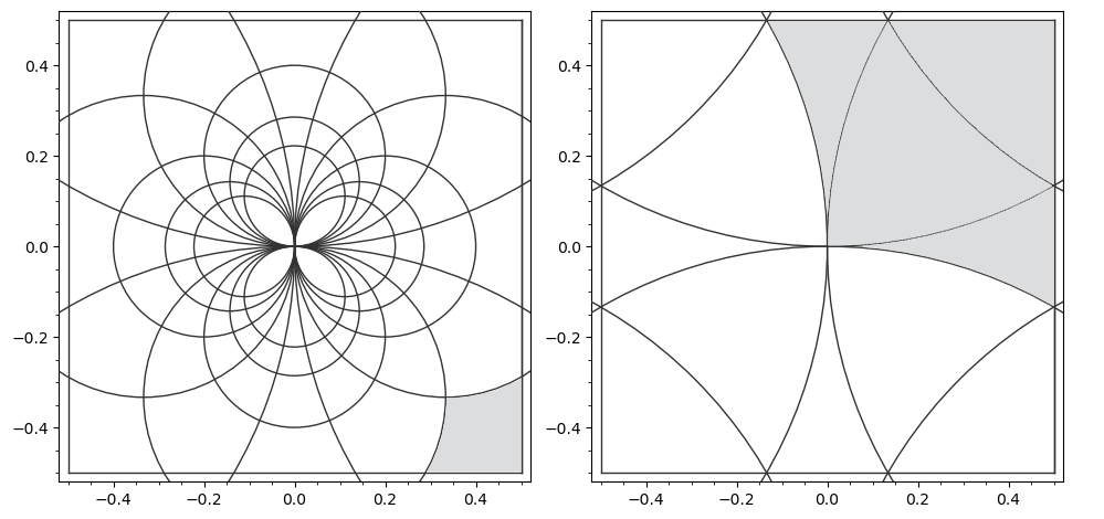
Figure 1. Partition element $O_{1+i}$ and image $TO_{1+i}$ (as a disjoint union of cells in a finite partition ${{\mathcal{P}}}$) depicted in grey ($d=1$).

1.4. Transfer operators associated to $(I,T)$

We introduce the transfer operator.

Set ${\mathcal{A}}:=\{\alpha\in\mathcal{O}\colon\text{$O_{\alpha}$ is non-empty}\}$. For $\alpha\in\mathcal{A}$, the origin is not a limit point of $O_{\alpha}$, whence the inverse branch $h_{\alpha}\colon TO_{\alpha}\to O_{\alpha}$ extends holomorphically to an open neighborhood of $TO_{\alpha}$. The extension is unique since $TO_{\alpha}$ has non-empty interior for any $\alpha\in\mathcal{A}$. Denote by $h_{\alpha}^{\prime}$ the holomorphic derivative of $h_{\alpha}$. Under the identification $\mathbb{C}\simeq\mathbb{R}^{2}$, we regard $h_{\alpha}$ as a $\mathbb{R}^{2}$-valued function and write $J_{\alpha}$ for its Jacobian determinant. As a consequence of the Cauchy–Riemann equation, we have

(1.4) $$J_{\alpha}(z)=\left|h_{\alpha}^{\prime}(z)\right|^{2}.$$

In particular, $J_{\alpha}(z)>0$ for all $z\in TO_{\alpha}$.

By a digit cost $c$, which mean a function on ${\mathcal{A}}$ such that $c(\alpha)\geq 0$ for all $\alpha\in\mathcal{A}$. Abusing the notation, we also regard $c$ as a function on $I$, by letting $c(z):=c({\alpha})$ for $z\in O_{\alpha}$.

Definition 1.5.

Let $s$ and $w$ be complex parameters. For a digit cost $c$, define $g_{s,w}(z):=\exp(wc(z))J_{[z^{-1}]}(T(z))^{s}$. For a function $f:I\rightarrow\mathbb{C}$, the weighted transfer operator is defined by

$$\mathcal{L}_{s,w}f(z) :=\sum_{T(z_{0})=z}g_{s,w}(z_{0})f(z_{0}).$$

Due to the properties of inverse branches in §1.2, we have

(1.5) $$\mathcal{L}_{s,w}f(z)=\sum_{{\alpha}\in{\mathcal{A}}}g_{s,w}(z)\cdot(f\circ h_{\alpha})(z)\cdot 1_{TO_{\alpha}}(z).$$

To proceed, we settle a few notations. For a subset $P\in\mathcal{P}$ of $TO_{\alpha}$, denote the restriction of $h_{\alpha}$ to $P$ by $\langle\alpha\rangle^{P}_{Q}\colon P\to Q$ if $h_{\alpha}(P)\subset Q$. For $P,Q\in\mathcal{P}$, set

$$\mathcal{H}(P,Q)=\left\{h\colon P\to Q:\text{ $h=\langle\alpha\rangle^{P}_{Q}$ for some $\alpha\in\mathcal{O}$}\right\}$$

to be the collection of restricted inverse branch maps from $P$ to $Q$. Then by Proposition  A, (1.5) becomes, for $z\in P$

(1.6) $$\left(\mathcal{L}_{s,w}f\right)_{P}(z)=\sum_{Q\in{{\mathcal{P}}}}\sum_{\langle\alpha\rangle^{P}_{Q}\in\mathcal{H}(P,Q)}g_{s,w}(z)\cdot\left(f_{Q}\circ\langle\alpha\rangle^{P}_{Q}\right)(z).$$

This shows that if ${{\mathcal{P}}}$ is compatible with $T$ and (1.6) is convergent for each $P$, then the operator $\mathcal{L}_{s,w}$ preserves $C^{1}(\mathcal{P})$. To ensure the convergence, we assume a moderate growth assumption on the digit cost $c$; See (4.1).

1.5. Main results

We study the spectral properties of $\mathcal{L}_{s,w}$ acting on a Banach space $C^{1}(\mathcal{P})$ with respect to a family of norms $\|\cdot\|_{(t)}$ parametrised by a non-zero $t\in\mathbb{R}$. The norm takes the form

(1.7) $$\|f\|_{(t)}=\|f\|_{0}+\frac{1}{|t|}\|f\|_{1}$$

where $\|\!\cdot\!\|_{0}$ is essentially the sup-norm and $\|\!\cdot\!\|_{1}$ is a semi-norm; See §4.1 for the precise definition.

Write $s=\sigma+it$ and $w=u+i\tau$, with $\sigma,t,u,\tau\in\mathbb{R}$. We establish the following key facts, namely the Ruelle–Perron–Frobenius Theorem and a Dolgopyat-type uniform estimate.

Theorem B (Theorem 4.7 and 6.1).

For $(s,w)$ with $(\sigma,u)$ close to $(1,0)$,

1. For $(s,w)$ near $(1,0)$, there is a spectral gap, in particular, ${\mathcal{L}}_{s,w}$ has an eigenvalue $\lambda_{s,w}$ of maximal modulus and there are no other eigenvalues on the circle of radius $|\lambda_{s,w}|$, and $\lambda_{s,w}$ is algebraically simple.

2. For a suitable $\xi>0$ and sufficiently large $|t|$,

   $$\|(I-{\mathcal{L}}_{s,w})^{-1}\|_{(t)}\ll|t|^{\xi}.$$

The implied constant is determined by a real neighborhood of $(\sigma,u)=(1,0)$. See the paragraph above (4.1) for details.

Part (1) is obtained by so-called Lasota–Yorke inequality with topological mixing property of $(I,T)$. For the Dolgopyat estimate (2), the main steps are parallel to those of Baladi–Vallée [4] but we deal with technical difficulties that arise from higher dimensional nature of complex continued fractions. In particular, our proof relies on the analysis due to Ei–Nakada–Natsui [17] of the natural invertible extension of $(I,T)$ as well as a version of Van der Corput Lemma in dimension 2. See §6 for details.

Consequently, we obtain a Central Limit Theorem for the complex Gauss system $(I,T)$. Recall that for $z\in I$, we have the continued fraction expansion $z=[0;{\alpha}_{1},{\alpha}_{2},\ldots,{\alpha}_{n},\ldots]$, which terminates uniquely in a finite step $\ell(z)$ if $z\in I\cap K$. Define

$$C_{n}(z) :=\sum_{j=1}^{n}c({\alpha}_{j})\mbox{ for $z\in I$, and }$$

$$C(z) :=\sum_{j=1}^{\ell(z)}c({\alpha}_{j})\mbox{ for $z\in I\cap K$.}$$

We regard $C_{n}$ as a random variable on $I$. Theorem B.(1) leads to the following Gaussian distribution for continuous trajectories. Here, we use the convention that big-$O$ notation has an implied constant depending only on $(I,T)$ and ${{\mathcal{P}}}$.

Theorem C (Theorem 7.2).

Let $c$ be a digit cost satisfying the moderate growth assumption (4.1), which is not of the form $g-g\circ T$ for some $g\in C^{1}({{\mathcal{P}}})$. Let $\widehat{\mu}(c)$, $\widehat{\delta}(c)$, $\widehat{\mu}_{1}(c)$, and $\widehat{\delta}_{1}(c)$ be the certain constants given in the proof of Theorem 7.2.

For any $n\geq 1$ and $u\in\mathbb{R}$, the distribution of $C_{n}$ is asymptotically Gaussian;

$${\mathbb{P}}\left[\frac{C_{n}-\widehat{\mu}(c)n}{\widehat{\delta}(c)\sqrt{n}}\leq u\right]=\frac{1}{\sqrt{2\pi}}\int_{-\infty}^{u}e^{-\frac{t^{2}}{2}}dt+O\left(\frac{1}{\sqrt{n}}\right).$$

Also, the expectation and variance satisfy

$${\mathbb{E}}[C_{n}] =\widehat{\mu}(c)n+\widehat{\mu}_{1}(c)+O(\theta^{n})$$

$${\mathbb{V}}[C_{n}] =\widehat{\delta}(c)n+\widehat{\delta}_{1}(c)+O(\theta^{n})$$

for some $\theta<1$.

Now we regard $C$ as a random variable on a set of $K$-rational points with the bounded height, i.e., for a fixed $N\geq 1$,

$$\Omega_{N}:=\left\{z\in I\cap K\colon\mathrm{ht}(z)^{2}\leq N\right\}$$

where $\mathrm{ht}:K\rightarrow\mathbb{Z}_{\geq 0}$ denotes the height function on $K$; See (8.1).

Then Theorem B yields analytic properties of a Dirichlet generating series that is written in terms of resolvent of the operator ${\mathcal{L}}_{s,w}$. Applying a Tauberian argument, finally we obtain the uniform Quasi-power estimate for the moment generating function ${\mathbb{E}}_{N}[\exp(wC)|\Omega_{N}]$ for $w$ close to 0. In turn, we obtain the limit Gaussian distribution for rational trajectories, a generalisation of Theorem 1.1 over Euclidean imaginary quadratic fields:

Theorem D (Theorem 8.7).

Take $c$ as in Theorem C and further assume that it is bounded. Let $\mu(c)$, $\delta(c)$, $\mu_{1}(c)$, and $\delta_{1}(c)$ be the certain constants given in Theorem 8.7. For any $u\in\mathbb{R}$, the distribution of $C$ on $\Omega_{N}$ is asymptotically Gaussian;

$${\mathbb{P}}_{N}\left[\frac{C-\mu(c)\log N}{\delta(c)\sqrt{\log N}}\leq u\Big{\lvert}\,\Omega_{N}\right]=\frac{1}{\sqrt{2\pi}}\int_{-\infty}^{u}e^{-\frac{t^{2}}{2}}dt+O\left(\frac{1}{\sqrt{\log N}}\right).$$

Also, the expectation and variance satisfy

$${\mathbb{E}}_{N}[C|\Omega_{N}] =\mu(c)\log N+\mu_{1}(c)+O(N^{-\gamma})$$

$${\mathbb{V}}_{N}[C|\Omega_{N}] =\delta(c)\log N+\delta_{1}(c)+O(N^{-\gamma})$$

for some $\gamma>0$.

Here, we present another consequence, which is the estimate for ${\mathbb{E}}_{N}[\exp(i\tau C)|\Omega_{N}]$ for $\tau$ outside of the neighborhood of zero, which implies the following residual equidistribution. We remark that the result of this type was first given in Lee–Sun [24] for real continued fractions.

Theorem E (Theorem 9.2).

Take $c$ as in Theorem C. Further assume that $c$ is bounded and takes values in $\mathbb{Z}_{\geq 0}$. Let $q\geq 1$ be an integer. Then, the values of $C$ modulo $q$ are equidistributed on $\Omega_{N}$, i.e., for any $a\in\mathbb{Z}/q\mathbb{Z}$,

$${\mathbb{P}}_{N}[C\equiv a\ (\mathrm{mod}\ q)|\Omega_{N}]=q^{-1}+o(1).$$

Remark 1.6.

The boundedness assumption on $c$ in Theorem D and E is used in the proofs to deduce $C(z)=O(\log N)$ for $z\in\Omega_{N}$. This bound is stronger than what can be proved using the moderate growth condition, namely $C(z)=O(\log^{2}N)$, but simplifies the proofs by allowing us to use Theorem 8.3, the truncated Perron formula.

While the boundedness assumption is satisfied in the instances of our major interest, we note that the moderate growth condition is sufficient in the alternative approach [4, § 4] where the Perron formula without truncation is used in conjunction with the smoothing process.

This article is organised as folows. In §2, we study expanding, distortion properties of the complex Gauss dynamical system $(I,T)$. In §3, we show the existence of a finite Markov structure compatible with the countable inverse branches. In §4, we show quasi-compactness of the associated transfer operator acting on piecewise $C^{1}$-space, hence a spectral gap. In §5, we settle a priori bounds for the normalised family of operator which will be used in §6, where we have Dolgopyat-type estimate. In §7-8, we have limit Gaussian distributions for complex and rational trajectories. In §9, we obtain residual equidistribution.

Acknowledgements

We are grateful to Hans Henrik Rugh for the idea of Lemma 6.6. We also thank Hitoshi Nakada, Hiromi Ei, Rie Natsui for helpful discussion and sharing the preprint [17] with us, and Malo Jézéquel for clarifying comments.

2. Complex Gauss dynamical system

In this section, we note that the complex Gauss map admits uniform expanding and distortion properties. We point out that these estimates will be crucially used later for spectral analysis.

2.1. Metric properties of inverse branch

Recall that we denote an inverse branch of $T$ by $h_{\alpha}$ for some $\alpha\in{\mathcal{O}}$, which induces a bijection $TO_{\alpha}\to O_{\alpha}$. More generally, for a sequence ${\boldsymbol{\alpha}}=(\alpha_{1},\cdots,\alpha_{n})\in{\mathcal{O}}^{n}$, define $O_{\boldsymbol{\alpha}}$ inductively as

$$O_{(\alpha_{1},\alpha_{2})} =\left\{z\in O_{\alpha_{1}}\colon T(z)\in O_{\alpha_{2}}\right\}$$

$$\vdots$$

$$O_{(\alpha_{1},\cdots,\alpha_{n})} =\left\{z\in O_{\alpha_{1}}\colon T(z)\in O_{(\alpha_{2},\cdots,\alpha_{n})}\right\}.$$

It follows that $h_{\boldsymbol{\alpha}}:=h_{\alpha_{1}}\circ\cdots\circ h_{\alpha_{n}}$ induces a bijection $T^{n}O_{{\boldsymbol{\alpha}}}\to O_{{\boldsymbol{\alpha}}}$. Also, we call $n$ the depth of $h_{\boldsymbol{\alpha}}$. We call $\langle{\boldsymbol{\alpha}}\rangle_{Q}^{P}:=h_{{\boldsymbol{\alpha}}}|_{P}$ an inverse branch of depth $n$ from $P$ to $Q$ and denote by ${\mathcal{H}}^{n}(P,Q)$ the set of all such inverse branches. Note that $\langle{\boldsymbol{\alpha}}\rangle_{Q}^{P}$ extends uniquely to a conformal map on $\mathbb{C}\cup\{\infty\}$.

For $P,Q\in\mathcal{P}$, put

$$\mathcal{H}^{\star}(P,Q)=\bigcup_{n\geq 1}\mathcal{H}^{n}(P,Q)\ \mbox{ and }\ \mathcal{H}^{\star}=\bigcup_{P,Q\in\mathcal{P}}\mathcal{H}^{\star}(P,Q).$$

For $\langle{\boldsymbol{\alpha}}\rangle\in\mathcal{H}^{\star}(P,Q)$, denote by $|{\boldsymbol{\alpha}}|$ the integer satisfying $\langle{\boldsymbol{\alpha}}\rangle\in\mathcal{H}^{|{\boldsymbol{\alpha}}|}(P,Q)$ and call it again the depth of $\langle{\boldsymbol{\alpha}}\rangle$.

Observe that the inverse branches are conformal and have contracting properties. For sufficiently large $n$, we have

$$\sup_{|{\boldsymbol{\alpha}}|=n}\sup_{P\in\mathcal{P}}\sup_{z\in P}|J_{{\boldsymbol{\alpha}}}(z)|<1.$$

Define the contraction ratio to be the positive real number $\rho<1$ given by

(2.1) $$\rho:=\lim_{n\to\infty}\sup_{|{\boldsymbol{\alpha}}|=n}\sup_{z\in TO_{{\boldsymbol{\alpha}}}}|J_{{\boldsymbol{\alpha}}}(z)|^{1/n}.$$

It follows that $|J_{{{\boldsymbol{\alpha}}}}|\ll\rho^{|{\boldsymbol{\alpha}}|}.$ Since the Jacobian of $z\mapsto 1/z$ as a function on $\mathbb{R}^{2}$ is of the form $|z|^{-4}$, we obtain the following.

Proposition 2.1.

Suppose that the domain $I\subseteq\mathbb{C}$ is contained in an open ball centered at zero of radius $R$. Then, $\rho\leq R^{4}.$ In particular, $\rho<1$.

Proof.

For ${\alpha}\in\mathcal{A},$ recall (1.4) that we have

$$|J_{\alpha}(z)|=|h_{\alpha}^{\prime}(z)|^{2}=|h^{2}_{\alpha}(z)|^{2}\leq R^{4}.$$

The chain rule implies that $|J_{{\boldsymbol{\alpha}}}|\leq R^{4|{\boldsymbol{\alpha}}|}$. From this, we conclude $\rho\leq R^{4}$.

To see $\rho<1$, it suffices to observe $R\leq\sqrt{15/16}$ in all cases of $d$ we consider. ∎

2.2. Distortion estimate

Next we observe the following distortion property of inverse branches.

Proposition 2.2 (Bounded distortion).

There is a uniform constant $M>0$ such that for any $n$ and $h_{{\boldsymbol{\alpha}}}=h_{{\alpha}_{1}}\circ\cdots\circ h_{{\alpha}_{n}}$, and any unit tangent vector $v$,

$$|\partial_{v}J_{{\boldsymbol{\alpha}}}(z)|\leq 2M|J_{{\boldsymbol{\alpha}}}(z)|$$

for all $z\in T^{n}O_{\boldsymbol{\alpha}}$. Here $\partial_{v}$ denotes the directional derivative.

Proof.

Let $v=(v_{1}\frac{\partial}{\partial z},v_{2}\frac{\partial}{\partial\bar{z}})$ be a unit tangent vector in the complex plane so that $v_{1}^{2}+v_{2}^{2}=1/2$. Then for any $h_{{\alpha}}$, i.e., $n=1$, we have

$$\partial_{v}J_{\alpha}(z) =\partial_{v}|h^{\prime}_{\alpha}(z)|^{2}=v_{1}\cdot h^{\prime\prime}_{\alpha}(z)\overline{h^{\prime}_{\alpha}(z)}+v_{2}\cdot h^{\prime}_{\alpha}(z)\overline{h^{\prime\prime}_{\alpha}(z)}$$

and obtain

(2.2) $$\left|\frac{\partial_{v}J_{\alpha}(z)}{J_{\alpha}(z)}\right| =\left|\frac{v_{1}\cdot h^{\prime\prime}_{\alpha}(z)\overline{h^{\prime}_{\alpha}(z)}+v_{2}\cdot h^{\prime}_{\alpha}(z)\overline{h^{\prime\prime}_{\alpha}(z)}}{|h_{\alpha}^{\prime}(z)|^{2}}\right|$$

$$=\left|v_{1}\frac{h_{\alpha}^{\prime\prime}(z)}{h_{\alpha}^{\prime}(z)}+v_{2}\frac{\overline{h^{\prime\prime}_{\alpha}(z)}}{\overline{h^{\prime}_{\alpha}(z)}}\right|$$

$$\leq 4(v_{1}^{2}+v_{2}^{2})\left|\frac{h_{\alpha}^{\prime\prime}(z)}{h_{\alpha}^{\prime}(z)}\right|\leq\frac{2}{|z+{\alpha}|}$$

Note that for $z\in TO_{\alpha}$ and ${\alpha}\in{\mathcal{A}}$, $|z+{\alpha}|$ is bounded below by 1, since $z+{\alpha}$ lies in the exterior of union of circles given by inversion image of the boundaries of $I$ and the unit circle properly lies inside the union of these circles for all $d=1,2,3,7,11$). Hence, we have a uniform upper bound $\widehat{M}=\widehat{M}(d)>0$ for (2.2).

Suppose now $h_{{\boldsymbol{\alpha}}}=h_{{\alpha}_{1}}\circ\cdots\circ h_{{\alpha}_{n}}$ and $n>1$. Write $k_{n-i}=h_{{\alpha}_{i+1}}\circ\cdots\circ h_{{\alpha}_{n}}$. Then by the chain rule of complex derivative and contraction from Proposition 2.1,

$$\left|\frac{h_{\boldsymbol{\alpha}}^{\prime\prime}(z)}{h_{\boldsymbol{\alpha}}^{\prime}(z)}\right| =\left|\frac{(h_{{\alpha}_{1}}^{\prime\prime}\circ k_{n-1})(z)}{(h_{{\alpha}_{1}}^{\prime}\circ k_{n-1})(z)}\cdot k_{n-1}^{\prime}(z)+\frac{k_{n-1}^{\prime\prime}(z)}{k_{n-1}^{\prime}(z)}\right|$$

$$\leq\widehat{M}\rho^{\frac{n-1}{2}}+\left|\frac{(h_{{\alpha}_{2}}^{\prime\prime}\circ k_{n-2})(z)}{(h_{{\alpha}_{2}}^{\prime}\circ k_{n-2})(z)}\cdot k^{\prime}_{n-2}(z)+\frac{k_{n-2}^{\prime\prime}(z)}{k_{n-2}^{\prime}(z)}\right|$$

$$\leq\widehat{M}(\rho^{\frac{n-1}{2}}+\cdots+\rho^{\frac{1}{2}}+1)$$

inductively. This is uniformly bounded by the constant $M:=\frac{2\widehat{M}}{1-\rho^{1/2}}>0$. ∎

3. Finite Markov partition with cell structure

In this section, we recall the work of Ei–Nakada–Natsui [17] regarding the finite range structure of $(I,T)$,which leads to the existence of an absolutely continuous invariant measure and a dual fractal domain. Then we obtain a cell structure out of the finite partition $\mathcal{P}$ and show that this is indeed Markov and compatible with $T$ as in Definition 1.4.

3.1. Work of Ei–Nakada–Natsui

Let $W_{0}$ be the set of lines such that any $z\in\partial I$ is contained in some $w\in W_{0}$. That is each $w\in W_{0}$ is a line spanned by a side of $I$. If $w\subset\mathbb{C}$ is a line or a circle, we denote by $w^{-1}$ the line or the circle obtained as the image under the inversion map $z\mapsto 1/z$.

Now define $W_{n}$ for $n\geq 1$ inductively as follows. First, put

$${\mathcal{A}}(w)=\left\{\alpha\in{\mathcal{A}}\colon w^{-1}\cap\left(I+\alpha\right)\not=\emptyset\right\},$$

and define

(3.1) $$W_{1} :=\{w^{-1}-{\alpha}:w\in W_{0},\ {\alpha}\in{\mathcal{A}}(w)\}.$$

For $n\geq 1$, recursively define

$$W_{n} :=\{w^{-1}-{\alpha}:w\in W_{0}\cup\cdots\cup W_{n-1},\ {\alpha}\in{\mathcal{A}}(w)\}.$$

Ei–Nakada–Natsui [17, Theorem 2] showed that $W_{n}$ stabilises.

Theorem 3.1 (Ei–Nakada–Natsui [17]).

For the complex Gauss system $(I,T)$, there exists $n_{0}=n_{0}(d)\geq 1$ such that

$$W_{n_{0}+1}\subseteq\bigcup_{j=1}^{n_{0}}W_{j}.$$

Moreover, $W_{j}$ is finite for each integer $j\geq 1$.

In fact, we have $n_{0}(1)=n_{0}(3)=1$, $n_{0}(2)=2$, and $n_{0}(7)=n_{0}(11)=4$. See [17, §4.3] for a complete list of equations for the lines and circles in $W_{n_{0}}$.

Definition 3.2.

Let ${{\mathcal{P}}}[2]$ be the set of connected components of $I-\cup_{j=1}^{n_{0}}W_{j}$.

Example 3.3 ($d=1$).

The set $W_{0}$ contains the lines $\ell_{1}^{\pm}:\mathrm{Re}(z)=\pm 1/2$ and $\ell_{2}^{\pm}:\mathrm{Im}(z)=\pm 1/2$. Then the step (3.1) induces the circles $C_{1}^{\pm}:|z\pm 1|=1$, $C_{2}^{\pm}:|z\pm i|=1$, $C_{3}^{\pm}:|z\pm(1+i)|=1$, and $C_{4}^{\pm}:|z\pm(1-i)|=1$ in $W_{1}$.

Then we see, under the inversion map, $\ell_{1}^{\pm}$ maps to $C_{1}^{\mp}$, $\ell_{2}^{\pm}$ maps to $C_{2}^{\mp}$, and $C_{3}^{\pm}$ maps to $C_{4}^{\mp}$. Hence, $W_{2}=W_{1}$ and $n_{0}=1$.

Based on Theorem 3.1, Ei–Nakada–Natsui [17, §5] constructed the natural extension $\widetilde{T}$ of $T$ on $\mathbb{C}^{2}$ and found a subset $\bigcup_{P\in{{\mathcal{P}}}}P\times P^{*}$ on which $\widetilde{T}$ is one-to-one and onto. Here, $P^{*}$ is defined to be the closure of the set

(3.2) $$\bigcup_{n\geq 1}\left\{\widetilde{T}^{n}(z,0)\colon z\in P\right\}.$$

Accordingly, this yields the density function of an absolutely continuous invariant measure for $(I,T)$ and a bounded fractal domain $I^{*}=\cup_{P\in{{\mathcal{P}}}}P^{*}$ which is contained in the closed unit disc.

In view of continued fraction expansion, if the sequence of digits ${\boldsymbol{\alpha}}=({\alpha}_{1},\cdots,{\alpha}_{n})$ is an expansion for $z\in I$, then the backward sequence ${\boldsymbol{\alpha}}^{*}=({\alpha}_{n},\cdots,{\alpha}_{1})$ is also an admissible expansion for some $w\in I^{*}$. We denote by $h_{{\boldsymbol{\alpha}}^{*}}$ the corresponding inverse branch and call this the dual inverse branch. We remark that it satisfies the same distortion properties as in Proposition 2.2 due to the boundedness of $I^{*}$. Further, we notice the following estimates, which will be crucially used later in §6.2 to have Uniform Non-Integrability.

Denote by $\mathrm{Leb}$ the Lebesgue measure on $\mathbb{R}^{2}$. For $z\in I$, write $\frac{P_{n}}{Q_{n}}=[0;{\alpha}_{1},\ldots,{\alpha}_{n}]$ for the $n$-th convergent. Remark that we have $\frac{Q_{n-1}}{Q_{n}}=[0;{\alpha}_{n},\ldots,{\alpha}_{1}]$.

Proposition 3.4.

For $d\in\{1,2,3,7,11\}$, there is a positive constant $R=R_{d}<1$ such that for $h_{{\boldsymbol{\alpha}}^{*}}\in{\mathcal{H}}^{*n}$ and $P\in\mathcal{P},$

1. $\mathrm{Diam}(h_{{\boldsymbol{\alpha}}^{*}}(P^{*}))\leq R^{2(n-1)}|1-R|^{-1}.$

2. $\mathrm{Leb}(h_{{\boldsymbol{\alpha}}^{*}}(P^{*}))\leq\left(R^{2(n-1)}|1-R|^{-1}\right)^{2}$.

Proof.

Let $C_{d}=1/R_{d}$, where $R_{d}<1$ is the minimal radius of the ball containing $I_{d}$ centered at the origin. Since $Q^{*}_{n-1}/Q^{*}_{n}\in I_{d},$ it follows that $C_{d}|Q^{*}_{n-1}|<|Q^{*}_{n}|$. For instance, we have $C_{1}=\sqrt{2}.$

Following Ei–Ito–Nakada–Natsui [15] (which covers the case $d=1$), we have

$$\left|w-\frac{P^{*}_{n}}{Q^{*}_{n}}\right| \leq\frac{1}{|Q^{*}_{n}|^{2}\left|1+T^{n}_{d}(w)\frac{Q^{*}_{n-1}}{Q^{*}_{n}}\right|}$$

$$\leq\frac{1}{|Q^{*}_{n}|^{2}||1-1/C_{d}|}\leq R_{d}^{2(n-1)}|1-R_{d}|^{-1}.$$

Then (2) follows immediately from (1). ∎

Proposition 3.5.

There exist $L_{1},L_{2}>0$ such that for any $n\geq 1$ and $h_{\boldsymbol{\alpha}}\in{\mathcal{H}}^{n}$, all $z_{1},z_{2}\in I$,

$$L_{1}\leq\left|\frac{h_{\boldsymbol{\alpha}}^{\prime}(z_{1})}{h_{{\boldsymbol{\alpha}}}^{\prime}(z_{2})}\right|\leq L_{2}.$$

The same property holds for the dual inverse branch $h_{{\boldsymbol{\alpha}}^{*}}\in{\mathcal{H}}^{*n}$.

Proof.

Notice that $h_{\boldsymbol{\alpha}}$ with an admissible ${\boldsymbol{\alpha}}=({\alpha}_{1},\cdots,{\alpha}_{n})$ corresponds to ${\mathrm{GL}}_{2}({\mathcal{O}})$ matrices with determinant $\pm 1$,

$$\left[\begin{matrix}0&1\\ 1&{\alpha}_{1}\end{matrix}\right]\cdots\left[\begin{matrix}0&1\\ 1&{\alpha}_{n}\end{matrix}\right]=\left[\begin{matrix}P_{n-1}&P_{n}\\ Q_{n-1}&Q_{n}\end{matrix}\right].$$

Thus we have $h_{\boldsymbol{\alpha}}(z)=\frac{P_{n-1}z+P_{n}}{Q_{n-1}z+Q_{n}}$ and $h_{{\boldsymbol{\alpha}}^{*}}(z^{*})=\frac{P_{n-1}z^{*}+Q_{n-1}}{P_{n}z^{*}+Q_{n}}$, in turn we obtain the expression

(3.3) $$\left|\frac{h_{\boldsymbol{\alpha}}^{\prime}(z_{1})}{h_{{\boldsymbol{\alpha}}}^{\prime}(z_{2})}\right|=\left|\frac{\frac{Q_{n-1}}{Q_{n}}z_{2}+1}{\frac{Q_{n-1}}{Q_{n}}z_{1}+1}\right|^{2}\ \mbox{and }\left|\frac{h_{{\boldsymbol{\alpha}}^{*}}^{\prime}(z_{1}^{*})}{h_{{\boldsymbol{\alpha}}^{*}}^{\prime}(z_{2}^{*})}\right|=\left|\frac{\frac{P_{n}}{Q_{n}}z_{2}^{*}+1}{\frac{P_{n}}{Q_{n}}z_{1}^{*}+1}\right|^{2}.$$

Recall the triangle inequality that $||z_{1}|-|z_{2}||\leq|z_{1}+z_{2}|\leq|z_{1}|+|z_{2}|$ for any $z_{1},z_{2}\in\mathbb{C}$. Since ${\boldsymbol{\alpha}}$ and ${\boldsymbol{\alpha}}^{*}$ are admissible, we have $|\frac{P_{n}}{Q_{n}}|<R_{d}$, $|\frac{Q_{n-1}}{Q_{n}}|\leq 1$. Further for $j\in\{1,2\}$, $|z_{j}|<R_{d}$ and $|z_{j}^{*}|\leq 1$ as $I^{*}$ is a domain bounded by the unit circle. Hence (3.3) yields the final bounds, e.g., by taking $L_{2}=\frac{4}{|R_{d}-1|^{2}}$ and $L_{1}=\frac{1}{L_{2}}$. ∎

Remark 3.6.

The same argument yields

$$L_{1}\leq\left|\frac{h_{\boldsymbol{\alpha}}^{\prime}(z_{1})}{h_{{\boldsymbol{\alpha}}^{*}}^{\prime}(z_{2}^{*})}\right|\leq L_{2}$$

for all $z_{1}\in I$ and $z_{2}^{*}\in I^{*}$.

3.2. Existence of the finite Markov partition

We define ${{\mathcal{P}}}$ to be as follows. Recall that we have ${{\mathcal{P}}}[2]$ from Definition 3.2. Set

$${{\mathcal{P}}}[1] =\{(w\cap\overline{P})^{\circ}:w\in W_{0}\cup\cdots\cup W_{n_{0}},P\in{{\mathcal{P}}}[2]\}.$$

$${{\mathcal{P}}}[0] =I-\bigcup_{P\in{{\mathcal{P}}}[i]\atop i=1,2}P.$$

Then $\mathcal{P}:=\bigcup_{i=0}^{2}\mathcal{P}[i]$. Using Theorem 3.1, we claim that ${{\mathcal{P}}}$ is a Markov partition which is compatible with $T$ in the following sense.

Proposition 3.7.

For the cell structure ${{\mathcal{P}}}$ of $(I,T)$, we have

1. For each non-empty $O_{\alpha}$, $TO_{\alpha}$ is a disjoint union of cells in $\mathcal{P}$.

2. For each inverse branch $h_{\alpha}$ and $P\in\mathcal{P}$, either there is a unique member $Q\in\mathcal{P}$ such that $h_{\alpha}(P)\subset Q$ or $h_{\alpha}(P)$ is disjoint from $I$.

Proof.

(1) This is clear from the construction of $W_{n}$ from §3.1.

(2) Let $\overline{W}$ be the set of circles and lines which give the equations for all the elements of $\mathcal{P}[1].$ Thus it is enough to show that if $h_{\alpha}(P)\cap I\neq\emptyset$, then $h_{\alpha}\cap w=\emptyset$ for all $w\in\overline{W}.$

If $h_{\alpha}(P)\cap w\neq\emptyset$ for some $w\in\overline{W}$, then $\mathcal{O}_{\alpha}\cap w\neq\emptyset$ since $\mathcal{O}_{\alpha}$ contains $h_{\alpha}(P)$. It follows that $\mathcal{O}_{\alpha}^{-1}\cap w^{-1}\neq\emptyset$, which in turn implies that $(I+{\alpha})\cap w^{-1}\neq\emptyset.$ Thus ${\alpha}$ is one of the elements that are used in the inductive process of constructing $\overline{W}$. It follows that $w=h_{\alpha}(w^{\prime})$ for some $w^{\prime}\in\overline{W}$, since $\overline{W}$ is stable under the inductive process (3.1). In other words, $h_{\alpha}(P)\cap h_{\alpha}(w^{\prime})\neq\emptyset$, i.e., $(P+{\alpha})^{-1}\cap(w^{\prime}+{\alpha})^{-1}\neq\emptyset.$ Thus we conclude that $P\cap w^{\prime}\neq\emptyset$, which contradicts to the construction of the partition $\mathcal{P}$. See Figure 2. ∎

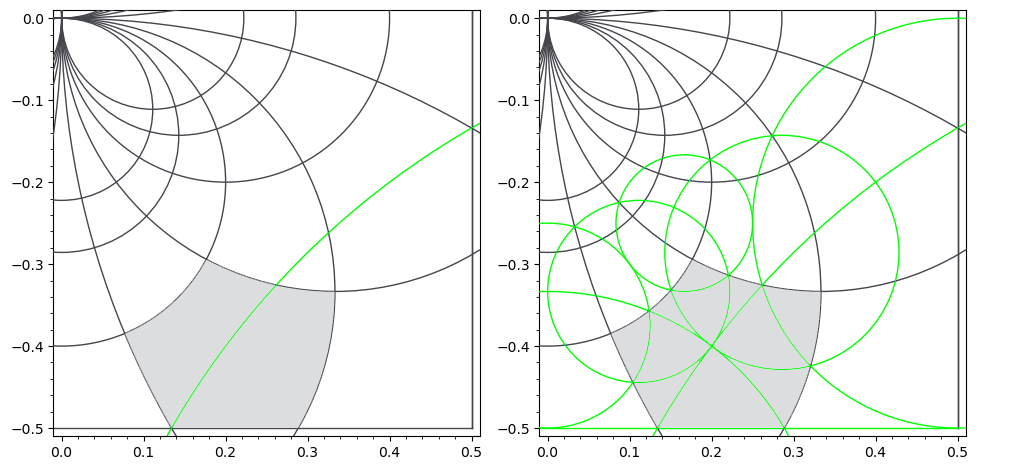
Figure 2. Boundary of cells in ${{\mathcal{P}}}$ induced by a circle in $W_{0}\cup W_{1}$ intersecting $I+(1+2i)$, and all images of $h_{1+2i}(P)$ inside $O_{1+2i}$ depicted in grey $(d=1)$.

4. Transfer operators on piecewise $C^{1}$-space

In this section, we study the spectrum of transfer operator ${\mathcal{L}}_{s,w}$ when $(s,w)$ is close to $(1,0)$. When ${\mathcal{L}}_{s,w}$ is acting on $C^{1}({{\mathcal{P}}})$, we show that the operator has a spectral gap with the dominant eigenvalue $\lambda_{s,w}$ which is unique and simple.

Throughout, write $s=\sigma+it$ and $w=u+i\tau$, and $r({\mathcal{L}})$ for the spectral radius of the operator ${\mathcal{L}}$. We say the digit cost $c$ is of moderate growth if $c({\alpha})=O(\log|{\alpha}|)$ for any ${\alpha}\in{\mathcal{A}}$. For such $c$, there exists a real neighborhood $K$ of $(1,0)\in\mathbb{R}^{2}$ such that for any $(s,w)$ with $(\sigma,u)\in K$, the series

(4.1) $$\sum_{\langle\alpha\rangle^{P}_{Q}\in\mathcal{H}(P,Q)}\exp\left(wc(\alpha)\right)|J_{\alpha}|^{s}$$

converges for all $P,Q\in\mathcal{P}$. Then we have $A_{K}>0$, depending only on $K$, such that the absolute value of (4.1) is bounded by $A_{K}$.

4.1. Function space: Norms on $C^{1}(\mathcal{P})$

We show that Proposition 3.7 allows us to consider the space of piecewise continuously differentiable functions, on which the ${\mathcal{L}}_{s,w}$ acts properly.

Definition 4.1.

Define $C^{1}(\mathcal{P})$ to be the space of functions $f\colon I\to\mathbb{C}$ such that for every $P\in\mathcal{P}$, $f|_{P}$ extends to a continuously differentiable function on on an open neighborhood of $\overline{P}$.

Denote the extension of $f_{P}$ to $\overline{P}$ by $\operatorname{res}_{P}(f)$. By the uniqueness of such an extension, it defines a linear map $\operatorname{res}_{P}\colon C^{1}(\mathcal{P})\to C^{1}(\overline{P})$. They collectively define a linear map $\operatorname{res}_{\mathcal{P}}:C^{1}(\mathcal{P})\rightarrow\bigoplus_{P\in\mathcal{P}}C^{1}(\overline{P})$ given by $f\mapsto\left(\operatorname{res}_{P}\left(f\right)\right)_{P\in\mathcal{P}}$.

Proposition 4.2.

The map $\operatorname{res}_{\mathcal{P}}$ is a bijection.

Proof.

We show that $\operatorname{res}_{\mathcal{P}}$ is an isomorphism by constructing an inverse. For each $f_{P}\in C^{1}(\overline{P})$ let $\tilde{f}_{P}\colon I\to\mathbb{C}$ be the function defined as

$$\tilde{f}_{P}(z)=\begin{cases}f_{P}(z)&\text{if $z\in P$,}\\ 0&\text{if $z\not\in P$.}\end{cases}$$

Define $j\colon\bigoplus_{P\in\mathcal{P}}C^{1}(\overline{P})\to C^{1}(\mathcal{P})$ by sending $(f_{P})_{P\in\mathcal{P}}$ to $\sum_{P\in\mathcal{P}}\tilde{f}_{P}$. Since $\mathcal{P}$ is a set-theoretic partition of $I$, the restriction of $\sum_{P\in\mathcal{P}}\tilde{f}_{P}$ to a given $P\in\mathcal{P}$ agrees with $f_{P}$ on $P$. Thus, $\sum_{P\in\mathcal{P}}\tilde{f}_{P}$ belongs to $C^{1}(\mathcal{P})$. Once we have defined $j$, it is easy to verify that $\operatorname{res}_{\mathcal{P}}\circ j$ and $j\circ\operatorname{res}_{\mathcal{P}}$ are identity maps, respectively. ∎

Let $\mathcal{P}[i]\subset\mathcal{P}$ be the set of open $i$-cells for $i=0,1,2$. Consider the following norms and semi-norms on $C^{1}(\mathcal{P}[i])$ for each $i=0,1,2$. For $P\in\mathcal{P}$ and $f_{P}\in C^{1}(\overline{P})$, define

$$\|f_{P}\|_{0}:=\sup_{z\in P}\left|f_{P}(z)\right|.$$

For a positive-dimensional cell $P$, define

$$\|f_{P}\|_{1}=\sup_{z\in P}\sup_{v}\left|\partial_{v}f_{P}(z)\right|$$

where the inner supremum is taken over the set of all unit tangent vectors $v$ with directional derivative $\partial_{v}$. When the dimension of $P$ is zero, there is no such tangent vector and we adopt the convention that $\|f_{P}\|_{1}=0$.

For $t\neq 0$, put

$$\|f_{P}\|_{(t)}=\|f_{P}\|_{0}+\frac{1}{|t|}\|f_{P}\|_{1}.$$

By abusing the notation, we equip $C^{1}({{\mathcal{P}}})$ with following norms. For $f=(f_{P})_{P}$ and $k=0,1$, set

(4.2) $$\|f\|_{k} =\sup_{P\in\mathcal{P}}\|f_{P}\|_{k}$$

(4.3) $$\|f\|_{(t)} =\|f\|_{0}+\frac{1}{|t|}\|f\|_{1}.$$

Remark that $\|\cdot\|_{1}$ is only a semi-norm, while both $\|\cdot\|_{0}$ and $\|\cdot\|_{(t)}$ are norms on $C^{1}(\mathcal{P})$ with which $C^{1}({{\mathcal{P}}})$ is a Banach space. We refer to e.g., Brezis [7, Proposition 8.1] for $C^{1}$-norm, and remark that the norm $\|\cdot\|_{(t)}$ is equivalent to $\|\cdot\|_{(1)}$ for any non-zero $t$.

Decompose $\mathcal{L}_{s,w}$ as the sum of component operators

(4.4) $$\mathcal{L}^{i}_{j,(s,w)}\colon C^{1}(\mathcal{P}[i])\to C^{1}(\mathcal{P}[j])$$

with $0\leq i,j\leq 2$. In particular, $\mathcal{L}^{i}_{j,(s,w)}=0$ whenever $j>i$. We first study the real parameter family ${\mathcal{L}}_{\sigma,u}$ and obtain the boundedness.

Proposition 4.3.

For $(\sigma,u)\in K$, we have ${\mathcal{L}}_{\sigma,u}(C^{1}({{\mathcal{P}}}))\subset C^{1}({{\mathcal{P}}})$ and the operator norm $\|{\mathcal{L}}_{\sigma,u}\|_{(1)}\leq\widehat{A}_{K}$ with $\widehat{A}_{K}>0$.

Proof.

This is a straightforward calculation using (4.1) and (2.1), similar to Proposition 4.6 below, by taking $\widehat{A}_{K}=|{{\mathcal{P}}}|A_{K}(1+|\sigma|+R^{4})$. ∎

4.2. Sufficient conditions for quasi-compactness

The following is a sufficient criterion for the quasi-compactness of the bounded linear operators on a Banach space due to Hennion [18, Theorem XIV.3]:

Theorem 4.4 (Hennion).

Let $(B,\|\cdot\|)$ be a Banach space. Let $\|\cdot\|^{\prime}$ be a continuous semi-norm on $B$ and ${\mathcal{L}}$ a bounded linear operator on $B$ such that

1. The set $\left\{{\mathcal{L}}(f)\colon f\in B,\|f\|\leq 1\right\}$ is pre-compact in $(B,\|\!\cdot\!\|^{\prime})$.

2. For $f\in B$, $\|{\mathcal{L}}f\|^{\prime}\ll\|f\|^{\prime}$.

3. There exist $n\geq 1$, and real positive numbers $r$ and $C$ such that for $f\in B$,

   (4.5) $$\|{\mathcal{L}}^{n}f\|\leq r^{n}\|f\|+C\|f\|^{\prime}\mbox{ and }r<r({\mathcal{L}}).$$

Then ${\mathcal{L}}$ is quasi-compact, i.e., there is $r_{e}<r({\mathcal{L}})$ such that the part of its spectrum outside the disc of radius $r_{e}$ is discrete.

We remark that the two-norm estimate in (3) is so-called Lasota–Yorke (or Doeblin–Fortet, Ionescu–Tulcea and Marinescu) inequality. In this subsection, we verify the conditions of Hennion’s criterion for the quasi-compactness of the operator ${\mathcal{L}}_{\sigma,u}$ on $C^{1}({{\mathcal{P}}})$.

We immediately have (2) with $\|{\mathcal{L}}_{\sigma,u}\|_{0}\leq|{{\mathcal{P}}}|A_{K}$. Further, we observe the following compact inclusion, which implies (1) that $\|\cdot\|_{(1)}$ is pre-compact in $\|\cdot\|_{0}$.

Lemma 4.5.

The embedding $(C^{1}(\mathcal{P}),\|\cdot\|_{(1)})\rightarrow(C^{1}(\mathcal{P}),\|\cdot\|_{0})$ is a compact operator.

Proof.

It suffices to show that $(C^{1}(\mathcal{P}[i]),\|\!\cdot\!\|_{(1)})\rightarrow(C^{1}(\mathcal{P}[i]),\|\!\cdot\!\|_{0})$ is compact for each $i=0,1,2$. When $i=0$, it follows from the Bolzano–Weierstrass theorem. For $i=1,2$, it follows from the Arzelà–Ascoli theorem. ∎

Finally we obtain the key Lasota–Yorke estimate in (3). This will be also useful for the later purpose.

Proposition 4.6.

For $f\in C^{1}({{\mathcal{P}}})$ and $n\geq 1$, we have

$$\|{\mathcal{L}}^{n}_{\sigma,u}f\|_{(1)}\leq C_{K}(|\sigma|\|f\|_{0}+\rho^{n}\|f\|_{(1)})$$

for some $C_{K}>0$, depending only on $K$, where $\rho<1$ denotes the contraction ratio.

Proof.

It suffices to check for a positive dimensional $P$. Let $v=(v_{1}\frac{\partial}{\partial z},v_{2}\frac{\partial}{\partial\bar{z}})$ be a unit tangent vector with $v_{1}^{2}+v_{2}^{2}=1/2$. Recall that for any $\langle\alpha\rangle^{P}_{Q}\in\mathcal{H}(P,Q)$ and $z\in P$,

$$\partial_{v}J_{\alpha}(z) =\partial_{v}|(h^{\prime}_{\alpha})(z)|^{2}=v_{1}(h^{\prime\prime}_{\alpha})(z)(\overline{h^{\prime}}_{\alpha})(z)+v_{2}(h^{\prime}_{\alpha})(z)(\overline{h^{\prime\prime}}_{\alpha})(z).$$

Recall the notation that for $\langle{\boldsymbol{\alpha}}\rangle\in{\mathcal{H}}^{n}(P,Q)$, $\langle{\boldsymbol{\alpha}}\rangle=\langle{\alpha}_{n}\rangle_{Q}^{R_{n-1}}\circ\cdots\circ\langle{\alpha}_{1}\rangle_{R_{1}}^{P}$ for some $R_{1},\cdots,R_{n-1}\in{{\mathcal{P}}}$. We put $c({\boldsymbol{\alpha}}):=\sum_{j=1}^{n}c({\alpha}_{j})$. For $n\geq 1$, we have

$$({\mathcal{L}}^{n}_{\sigma,u}f)_{P}(z)=\sum_{Q}\sum_{\langle{\boldsymbol{\alpha}}\rangle\in{\mathcal{H}}^{n}(P,Q)}e^{uc({\boldsymbol{\alpha}})}|J_{\boldsymbol{\alpha}}(z)|^{\sigma}\cdot f_{Q}\circ\langle{\boldsymbol{\alpha}}\rangle(z).$$

Thus we have

$$|\partial_{v}({\mathcal{L}}_{\sigma,u}^{n}f)_{P}(z)| \leq\left|\sum_{Q}\sum_{\langle{\boldsymbol{\alpha}}\rangle}e^{uc({\boldsymbol{\alpha}})}\partial_{v}|J_{\boldsymbol{\alpha}}(z)|^{\sigma}\cdot f_{Q}\circ\langle{\boldsymbol{\alpha}}\rangle(z)\right|$$

$$+\left|\sum_{Q}\sum_{\langle{\boldsymbol{\alpha}}\rangle}e^{uc({\boldsymbol{\alpha}})}|J_{\boldsymbol{\alpha}}(z)|^{\sigma}\cdot\partial_{v}(f_{Q}\circ\langle{\boldsymbol{\alpha}}\rangle)(z)\right|$$

$$\ll\left(\sum_{Q}\sum_{\langle{\boldsymbol{\alpha}}\rangle}e^{uc({\boldsymbol{\alpha}})}|\sigma||J_{\boldsymbol{\alpha}}(z)|^{\sigma}\left|\frac{\partial_{v}J_{\boldsymbol{\alpha}}(z)}{J_{\boldsymbol{\alpha}}(z)}\right|\cdot|f_{Q}\circ\langle{\boldsymbol{\alpha}}\rangle(z)|\right)$$

$$+\left(\sum_{Q}\sum_{\langle{\boldsymbol{\alpha}}\rangle}e^{uc({\boldsymbol{\alpha}})}|J_{\boldsymbol{\alpha}}(z)|^{\sigma}\cdot 2|J_{\boldsymbol{\alpha}}(z)|\cdot|\partial_{v}f_{Q}\circ\langle{\boldsymbol{\alpha}}\rangle(z)|\right).$$

The first term is then bounded by $\widetilde{A}_{K}M|\sigma|\|f\|_{0}$ and the second term is bounded by $\widetilde{A}_{K}\rho^{n}\|f\|_{1}$ (for a suitable $\widetilde{A}_{K}>0$ due to moderate growth (4.1)), where $\rho$ from Proposition 2.1 and $M$ from Proposition 2.2. By taking supremum and maximum on both sides, we obtain the inequality for some $C_{K}>0$. ∎

4.3. Ruelle–Perron–Frobenius Theorem

In this subsection, we conclude the quasi-compactness by §4.2, and in turn obtain the following Ruelle–Perron–Frobenius theorem, i.e., spectral gap for ${\mathcal{L}}_{\sigma,u}$ on $C^{1}({{\mathcal{P}}})$.

Theorem 4.7.

For $(\sigma,u)\in K$, the operator $\mathcal{L}_{\sigma,u}$ on $C^{1}({{\mathcal{P}}})$ is quasi-compact. It has a real eigenvalue $\lambda_{\sigma,u}$ with the following properties:

1. The eigenvalue $\lambda_{\sigma,u}>0$ is unique and simple. If $\lambda$ is an eigenvalue other than $\lambda_{\sigma,u}$, then $|\lambda|<\lambda_{\sigma,u}$.

2. A corresponding eigenfunction $\psi_{\sigma,u}=(\psi_{\sigma,u,2},\psi_{\sigma,u,1},\psi_{\sigma,u,0})$ for $\lambda_{\sigma,u}$ is positive. That is, $\psi_{\sigma,u,j}>0$ for all $j=0,1,2$.

3. There exists a unique probability measure $\nu_{\sigma,u}$ such that it is absolutely continuous with the 2-dimensional Lebesgue measure and that the dual operator satisfies ${\mathcal{L}}_{\sigma,u}^{*}\nu_{\sigma,u}=\lambda_{\sigma,u}\nu_{\sigma,u}$.

4. In particular, $\lambda_{1,0}=1$ and the density function for $\nu_{1,0}$ is $\psi_{1,0,2}$

Proof.

First we prove the quasi-compactness using Theorem 4.4. The required estimate (4.5) for some $n$ would follow from Proposition 4.6 if $\rho<r(\mathcal{L}_{\sigma,u})$ for any $(\sigma,u)\in K$. Since $r(\mathcal{L}_{\sigma,u})=r(\mathcal{L}_{\sigma,u}^{*})$, where $\mathcal{L}_{\sigma,u}^{*}$ is the dual operator, it suffices to prove $\rho<r(\mathcal{L}_{\sigma,u}^{*})$. Indeed, observe that the change of variable formula implies

(4.6) $$\int_{I}{\mathcal{L}}_{1,0}f(x,y)dxdy=\int_{I}f(x,y)dxdy$$

for any $f\in C^{1}({{\mathcal{P}}})$, which means $1\in\mathrm{Sp}({\mathcal{L}}_{1,0}^{*})$. By the analyticity of $r(\mathcal{L}_{\sigma,u}^{*})$ in $(\sigma,u)$, we conclude $\rho<r(\mathcal{L}_{\sigma,u}^{*})$ for any $(\sigma,u)\in K$, when we choose a sufficiently small $K$.

To proceed, we state and prove some $L^{1}$-estimates. In view of Proposition 4.2, we have a decomposition

$$C^{1}({{\mathcal{P}}})=C^{1}({{\mathcal{P}}}[2])\oplus C^{1}({{\mathcal{P}}}[1])\oplus C^{1}({{\mathcal{P}}}[0])$$

and accordingly the operator ${\mathcal{L}}:={\mathcal{L}}_{\sigma,u}$ can be written as

$${\mathcal{L}}f=\begin{bmatrix}{\mathcal{L}}_{2}^{2}&0&0\\ {\mathcal{L}}_{2}^{1}&{\mathcal{L}}_{1}^{1}&0\\ {\mathcal{L}}_{2}^{0}&{\mathcal{L}}_{1}^{0}&{\mathcal{L}}_{0}^{0}\end{bmatrix}\begin{bmatrix}f_{2}\\ f_{1}\\ f_{0}\end{bmatrix}$$

with ${\mathcal{L}}_{j}^{i}:C^{1}({{\mathcal{P}}}[i])\rightarrow C^{1}({{\mathcal{P}}}[j])$ from (4.4). Equip each $C^{1}(P)$ for $P\in\mathcal{P}[i]$ with the $L^{1}$-norm, by which we mean the $L^{1}$-norm with respect to the Lebesgue measure, $L^{1}$-norm with respect to the length element, and the counting measure, respectively for $i=2,1,0$. Define the $L^{1}$-norm on $C^{1}(\mathcal{P}[i])$ to be the sum of $L^{1}$-norms on its direct summands $C^{1}(P)$.

We claim, for $(\sigma,u)=(1,0)$,

(4.7) $$\|{\mathcal{L}}_{i}^{i}\|_{L^{1}} \leq R^{4-2i}\text{ for $i=2,1,0$.}$$

To obtain the case $i=2$, it suffices to prove $\|\mathcal{L}_{2}^{2}f\|_{L^{1}}\leq\|f\|_{L^{1}}$ for $f\in C^{1}(\mathcal{P}[2])$ by using the change of variable formula and the triangle inequality. To obtain the cases $i=1,0$ we use similar arguments. Consider the case $i=1$. By definition of ${\mathcal{L}}_{1}^{1}$, for $f\in L^{1}({{\mathcal{P}}}[1])$ and $P\in{{\mathcal{P}}}[1]$, we have

$$\|({\mathcal{L}}_{1}^{1}f)_{P}\|_{L^{1}}=\sum_{Q\in\mathcal{P}[1]}\int_{P}\left|\sum_{\langle\alpha\rangle\in{\mathcal{H}}(P,Q)}\left|z+\alpha\right|^{-4}\cdot f_{Q}\circ\langle\alpha\rangle(z)\right|d\ell_{P}$$

where $d\ell_{P}$ is the length element of the curve $P$. Applying the change of variable formula to the right hand side, we obtain

$$\|({\mathcal{L}}_{1}^{1}f)_{P}\|_{L^{1}}=\sum_{Q\in\mathcal{P}[1]}\int_{h_{\alpha}(P)}|z|^{2}|f_{Q}(z)|d\ell_{Q}.$$

Since $h_{\alpha}(P)$ are disjoint and $|z|\leq R$ for any $z\in I$, we conclude $\|\mathcal{L}_{2}^{2}f\|_{L^{1}}\leq\|f\|_{L^{1}}$.

Now consider the case $i=0$. For $P\in{{\mathcal{P}}}[0]$, we have

$$\|({\mathcal{L}}_{0}^{0}f)_{P}\|_{L^{1}}=\sum_{Q\in\mathcal{P}[0]}\left|\sum_{\langle\alpha\rangle\in{\mathcal{H}}(P,Q)}\left|z+\alpha\right|^{-4}\cdot f_{Q}\circ\langle\alpha\rangle(z)\right|$$

where $L^{1}({{\mathcal{P}}}[0])$-norm is given by the integral with respect to a counting measure. Again by the disjointness of $h_{\alpha}(P)$, we conclude $\|{\mathcal{L}}_{0}^{0}f\|_{L^{1}}\leq R^{4}\|f\|_{L^{1}}$.

By the density of $C^{1}(P)$ in the $L^{1}$-space, (4.7) yields, for $(\sigma,u)=(1,0)$, $r(\mathcal{L}_{i}^{i})\leq R^{4-2i}$ for $i=2,1,0$. It follows that

(4.8) $$r(\mathcal{L}_{2}^{2})>r(\mathcal{L}_{i}^{i})$$

for $i=0,1,$ and for all $(\sigma,u)\in K$. In particular, we have $r(\mathcal{L})=r(\mathcal{L}_{2}^{2})$.

We prove (1) in two steps. First, we prove the assertion for $\mathcal{L}_{2}^{2}$ when $(\sigma,u)\in K$. Lastly we prove the assertion for $\mathcal{L}$ when $(\sigma,u)\in K$. For the first step, we may adapt the proof of [3, Theorem 1.5.(4)]. We proceed to the second step. Note that if $(f_{2},f_{1},f_{0})$ is an eigenfunction of $\mathcal{L}$ then $f_{2}$ is an eigenfunction of $\mathcal{L}_{2}^{2}$ with the same eigenvalue. In particular, it induces a map from the $\lambda_{\sigma,u}$-eigenspace of $\mathcal{L}$ to that of $\mathcal{L}_{2}^{2}$. We claim that (4.8) implies that this is an isomorphism. Indeed, if $f_{2}$ is a $\lambda_{\sigma,u}$-eigenfunction for $\mathcal{L}_{2}^{2}$ then there is a unique way to complete it as a triple $(f_{2},f_{1},f_{0})$ which is an eigenfunction of $\mathcal{L}$. Concretely, $f_{1}$ and $f_{0}$ are determined by $f_{2}$ via the formulae

(4.9) $$f_{1}=\lambda_{\sigma,u}^{-1}(1-\lambda_{\sigma,u}^{-1}\mathcal{L}_{1}^{1})^{-1}(\mathcal{L}_{2}^{1}f_{2})$$

and

(4.10) $$f_{0}=\lambda_{\sigma,u}^{-1}(1-\lambda_{\sigma,u}^{-1}\mathcal{L}_{0}^{0})^{-1}(\mathcal{L}_{2}^{0}f_{2}+\mathcal{L}^{1}_{0}f_{1})$$

where the existence of $(1-\lambda_{\sigma,u}^{-1}\mathcal{L}_{i}^{i})^{-1}$ for $i=0,1$ follows from (4.8).

Now we prove (2). From the referred proofs [3, 19] for the fist step in the preceding paragraph, we know there is a $\lambda_{\sigma,u}$-eigenfunction $\psi_{\sigma,u,2}$ which is positive. The positivity of $\psi_{\sigma,u,2}$ together with the formulae (4.9) and (4.10) imply $\psi_{\sigma,u,1}>0$ and $\psi_{\sigma,u,0}>0$ in order. So $\psi_{\sigma,u,2}=(\psi_{\sigma,u,2},\psi_{\sigma,u,1},\psi_{\sigma,u,0})$ is the positive eigenfunction for $\mathcal{L}$, as desired.

We prove (3). This is nothing but an equivalent form of (1) in terms of the dual of a Banach space. We remark that for a bounded linear operator ${\mathcal{L}}$ on a Banach space, the notion of dual ${\mathcal{L}}^{*}$ is well-defined and $\lambda\in\mathrm{Sp}({\mathcal{L}})$ if and only if $\lambda\in\mathrm{Sp}({\mathcal{L}}^{*})$. The operator $\mathcal{L}^{*}$ is upper-triangular and its $\lambda_{\sigma,u}$-eigenspace is identified with that for $(\mathcal{L}_{2}^{2})^{*}$. The latter is further identified with a suitable measure space by the Riesz representation theorem, yielding the desired uniqueness.

To prove (4), it suffices to show $r(\mathcal{L}_{2}^{2})=1$ when $(\sigma,u)=(1,0)$, because we had proved that $r(\mathcal{L}_{2}^{2})=r(\mathcal{L})$. By (4.6), we have $r((\mathcal{L}_{2}^{2})^{*})\geq 1$ when $(\sigma,u)=(1,0)$. On the other hand, (4.7) implies $r((\mathcal{L}_{2}^{2})^{*})\leq 1$. We conclude $\lambda_{1,0}=1$. The assertion about the density function follows from the proof of (3). ∎

Remark 4.8.

Theorem 4.7.(4) can be viewed as an alternative proof of the main result of Ei–Nakada–Natsui [17] based on a thermodynamic formalism. However, their proof based on the construction of an invertible extension yields an integral expression for the density function $\psi_{1,0,2}$;

(4.11) $$\psi_{1,0,2}(z)=\int_{P^{*}}\frac{1}{|z-w|^{4}}d\mathrm{Leb}(w)$$

for $z\in P$, where $P\in{{\mathcal{P}}}[2]$. See also Hensley [19, Thm.5.5] for the case $d=1$.

We state some consequences of the assertion of Theorem 4.7 (1), whose proofs are referred to Kato [21, §VII.4.6, §IV.3.6]. First, there is a decomposition

$$\mathcal{L}_{s,w}=\lambda_{s,w}\mathcal{P}_{s,w}+\mathcal{N}_{s,w}$$

where $\mathcal{P}_{s,w}$ is a projection onto the $\lambda_{s,w}$-eigenspace and $\mathcal{N}_{s,w}$ satisfies both $r({\mathcal{N}}_{s,w})<|\lambda_{s,w}|$ and $\mathcal{P}_{s,w}\mathcal{N}_{s,w}=\mathcal{N}_{s,w}\mathcal{P}_{s,w}=0$. Moreover, $\lambda_{s,w}$, $\mathcal{P}_{s,w}$, and $\mathcal{N}_{s,w}$ vary analytically in $(s,w)$.

In particular, for a given $\varepsilon>0$, for any $(s,w)$ in a sufficiently small neighborhood $K$ of $(1,0)$, we have $r({\mathcal{N}}_{s,w})<|\lambda_{s,w}|-\varepsilon$. This yields

(4.12) $${\mathcal{L}}_{s,w}^{n}=\lambda_{s,w}^{n}{{\mathcal{P}}}_{s,w}+{\mathcal{N}}_{s,w}^{n}$$

where $r(|\lambda_{s,w}|^{-n}{\mathcal{N}}_{s,w}^{n})$ converges to zero as $n$ tends to infinity.

For the later purpose, we state the following.

Lemma 4.9.

The function $(s,w)\mapsto\lambda_{s,w}$ satisfies:

1. We have $\frac{\partial\lambda_{s,0}}{\partial s}\big{|}_{s=1}<0$, whence there is a complex neighborhood $W$ of 0 and unique analytic function $s_{0}:W\rightarrow\mathbb{C}$ such that for all $w\in W$,

   $$\lambda_{s_{0}(w),w}=1.$$

   In particular, $s_{0}(0)=1$.

2. We have $\frac{d^{2}}{dw^{2}}\lambda_{1+s_{0}^{\prime}(w)w,w}\big{|}_{w=0}\neq 0$ if and only if $c$ is not of the form $g-g\circ T$ for some $g\in C^{1}({{\mathcal{P}}})$.

Proof.

(1) Recall Theorem 4.7 and (4.12) that we have a spectral gap given by the identity ${\mathcal{L}}_{s,w}\psi_{s,w}=\lambda_{s,w}\psi_{s,w}$ and corresponding eigenmeasure $\nu_{s,w}$. We can assume that $\nu_{s,w}$ is normalised, i.e., $\int_{I}\psi_{s,w}d\nu_{s,w}=1$. Observe that

$${\mathcal{L}}_{s,w}\psi_{s,w} =\sum_{Q\in{{\mathcal{P}}}}\sum_{\langle\alpha\rangle\in{\mathcal{H}}(P,Q)}e^{wc({\alpha})}|J_{\alpha}|^{s}\cdot(\psi_{s,w})_{Q}\circ\langle\alpha\rangle$$

(4.13) $$={\mathcal{L}}_{1,0}(e^{wc}|J_{T}|^{1-s}\cdot\psi_{s,w})=\lambda_{s,w}\psi_{s,w}$$

where we regard $c$ as a function on $I$ given by $c(z):=c({\alpha})$ if $z\in O_{\alpha}$. Differentiating (4.13) with respect to $s$ and integrating with respect to $\nu_{1,0}$ yields the identity:

$$\frac{\partial\lambda_{s,0}}{\partial s}\bigg{|}_{s=1}=-\int_{I}\log|J_{T}|\psi_{1,0}d\nu_{1,0}.$$

From the right-hand-side, we see that it is negative from the positivity of $|J_{T}|$ and $\psi_{1,0}$. Then the existence of $s_{0}$ is obtained by implicit function theorem.

(2) This is a standard argument (convexity of the pressure) using a spectral gap as detailed in e.g., Parry–Pollicott [27, Proposition 4.9–4.12], Broise [8, Proposition 6.1], or Morris [25, Proposition 3.3]. Here, we briefly recall the main ideas.

Set $L(w):=\lambda_{1+s_{0}^{\prime}(w)w,w}$ and $\Psi(w):=\psi_{1+s_{0}^{\prime}(w)w,w}$. Notice that $L(0)=1$ and $L^{\prime}(0)=0$ by the mean value theorem. Similarly as (4.13), we have for any $n\geq 1$,

$${\mathcal{L}}_{1+s_{0}^{\prime}(w)w,w}^{n}\Psi(w)={\mathcal{L}}_{1,0}^{n}(e^{w\sum_{j=1}^{n}(c\circ T^{j-1})}|J_{T}|^{1-s}\cdot\Psi(w))=L(w)^{n}\Psi(w).$$

Differentiating this twice, setting $w=0$, and integrating gives

(4.14) $$L^{\prime\prime}(0)=\lim_{n\rightarrow\infty}\frac{1}{n}\int_{I}(\sum_{j=1}^{n}c\circ T^{j-1})^{2}\Psi(0)d\nu_{1,0}$$

with the use of limiting argument for $\Psi^{\prime}(0)$. Further, one can observe that the right hand side of (4.14) equals to $\int_{I}\widetilde{c}^{2}\Psi(0)d\nu_{1,0}$, where $\widetilde{c}:=c+g\circ T-g$ for some $g\in C^{1}({{\mathcal{P}}})$. Hence $L^{\prime\prime}(0)=0$ if and only if $\widetilde{c}=0$, which yields the final form of the statement. ∎

5. A priori bounds for the normalised family

In this section, we establish some a priori bounds, which will be crucially used for Dolgopyat–Baladi–Vallée estimate in the section 6.

For each $P\in{{\mathcal{P}}}$, normalise ${\mathcal{L}}_{s,w}$ by setting

(5.1) $$({\widetilde{\mathcal{L}}}_{s,w}f)_{P}=\frac{({\mathcal{L}}_{s,w}(\psi_{\sigma,u}\!\cdot\!f))_{P}}{\lambda_{\sigma,u}(\psi_{\sigma,u})_{P}}$$

where $\lambda_{\sigma,u}$ and $\psi_{\sigma,u}$ are from Theorem 4.7, and $(\psi_{\sigma,u})_{P}$ denotes the restriction of $\psi_{\sigma,u}$ to $P$. This satisfies ${\widetilde{\mathcal{L}}}_{\sigma,u}\bf 1=1$ and ${\widetilde{\mathcal{L}}}_{\sigma,u}^{*}$ fixes the probability measure $\mu_{\sigma,u}:=\psi_{\sigma,u}\nu_{\sigma,u}$.

5.1. Lasota–Yorke inequality

We begin with the Lasota–Yorke estimate and integral representation of the projection operator for the normalised family.

Lemma 5.1.

For $(s,w)$ with $(\sigma,u)\in K$, we have for $f\in C^{1}({{\mathcal{P}}})$ and some constant $\widetilde{C}_{K}>0$

1. $\|{\widetilde{\mathcal{L}}}_{s,w}^{n}f\|_{(1)}\leq\widetilde{C}_{K}(|s|\|f\|_{0}+\rho^{n}\|f\|_{(1)})$.

2. $\|{\widetilde{\mathcal{L}}}_{1,0}^{n}f\|_{0}=\int_{I}fd\mu_{1,0}+O(r_{1,0}^{n}\|f\|_{(1)})$.

Here $r_{s,w}$ denotes the spectral radius of $\frac{1}{\lambda_{\sigma,u}}{\mathcal{L}}_{s,w}-{{\mathcal{P}}}_{s,w}$.

Proof.

We prove (1). It is enough to show that

$$\|({\widetilde{\mathcal{L}}}_{s,w}^{n}f)_{P}\|_{(1)}\leq\widetilde{C}_{K}(|s|\|f\|_{0}+\rho^{n}\|f\|_{(1)})$$

for each $P$. If $P\in\mathcal{P}[0]$, then the left hand side involves no derivatives and the inequality holds for all sufficiently large $\tilde{C}_{K}$. Assume that $P$ is positive dimensional. Recalling that we put $c({\boldsymbol{\alpha}})=\sum_{j=1}^{n}c({\alpha}_{j})$, we divide $|\partial_{v}({\widetilde{\mathcal{L}}}_{s,w}^{n}f)_{P}|$ into three terms (i@), (ii@) and (iii@):

$$\lambda_{\sigma,u}^{-n}\cdot\frac{\partial_{v}(\psi_{\sigma,u})_{P}}{(\psi_{\sigma,u})_{P}^{2}}\sum_{Q}\sum_{\langle{\boldsymbol{\alpha}}\rangle}e^{wc({\boldsymbol{\alpha}})}|J_{\langle{\boldsymbol{\alpha}}\rangle}|^{s}\cdot(\psi_{\sigma,u}\!\cdot\!f)_{Q}\circ\langle{\boldsymbol{\alpha}}\rangle\quad(\textrm{\@slowromancap i@}),$$

$$\frac{\lambda_{\sigma,u}^{-n}}{(\psi_{\sigma,u})_{P}}\sum_{Q}\sum_{\langle{\boldsymbol{\alpha}}\rangle}e^{wc({\boldsymbol{\alpha}})}|s||J_{\langle{\boldsymbol{\alpha}}\rangle}|^{s-1}|\partial_{v}J_{\langle{\boldsymbol{\alpha}}\rangle}|\cdot(\psi_{\sigma,u}\!\cdot\!f)_{Q}\circ\langle{\boldsymbol{\alpha}}\rangle\quad(\textrm{\@slowromancap ii@})$$

and

$$\frac{\lambda_{\sigma,u}^{-n}}{(\psi_{\sigma,u})_{P}}\sum_{Q}\sum_{\langle{\boldsymbol{\alpha}}\rangle}e^{wc({\boldsymbol{\alpha}})}|J_{\langle{\boldsymbol{\alpha}}\rangle}|^{s}\left(f\!\cdot\!\partial_{v}\psi_{\sigma,u}+\psi_{\sigma,u}\!\cdot\!\partial_{v}f\right)_{Q}\circ\langle{\boldsymbol{\alpha}}\rangle.\quad(\textrm{\@slowromancap iii@})$$

Here, the inner sum is taken over $\langle{\boldsymbol{\alpha}}\rangle\in{\mathcal{H}}^{n}(P,Q)$, while the outer one is taken over $Q\in\mathcal{P}$.

The term (i@) is equal to $\left|\frac{\partial_{v}(\psi_{\sigma,u})_{P}}{(\psi_{\sigma,u})_{P}}({\widetilde{\mathcal{L}}}_{s,w}^{n}f)_{P}\right|$, whence it is bounded by $A_{K}\|{\widetilde{\mathcal{L}}}_{\sigma,u}^{n}|f|\|_{0}$ for some $A_{K}=\sup_{K}\|\psi_{\sigma,u}\|_{1}\|\psi_{\sigma,u}^{-1}\|_{0}$, which depends only on $K$ by perturbation theory. This is bounded by $A_{K}\|f\|_{0}$. The term (ii@) is bounded by $M|s|\|f\|_{0}$, where $M$ is the distortion constant in Proposition 2.2. The term (iii@) is bounded by $A_{K}\rho^{n}\|f\|_{0}+\rho^{n}\|f\|_{1}$, up to constant. Taking a suitable $\widetilde{C}_{K}>0$, we obtain (1).

We prove (2). Assume that eigenfunction and measure are normalised, i.e., $\int_{I}\psi_{\sigma,u}\nu_{\sigma,u}=1$. For $f\in\mathcal{C}^{1}({{\mathcal{P}}})$, we have for any $n\geq 1$

$$\mathcal{L}_{\sigma,u}^{n}f=\lambda_{\sigma,u}\!\cdot\!\psi_{\sigma,u}c(f)+{\mathcal{N}}^{n}_{\sigma,u}f$$

by the spectral decomposition (4.12). It follows that

$$\lambda_{\sigma,u}^{-n}\mathcal{L}_{\sigma,u}^{n}f=\psi_{\sigma,u}c(f)+\lambda_{\sigma,u}^{-n}{\mathcal{N}}_{\sigma,u}^{n}f,$$

which yields the identity $c(f)=\int_{I}fd\nu_{\sigma,u}$ by integrating against $\nu_{\sigma,u}$ and taking the limit as $n$ tends to infinity.

Due to the normalisation (5.1), we have

$${\widetilde{\mathcal{L}}}_{\sigma,u}^{n}f =\lambda_{\sigma,u}^{n}\psi_{\sigma,u}^{-1}{\mathcal{L}}_{\sigma,u}^{n}(\psi_{\sigma,u}\!\cdot\!f)$$

$$=\lambda_{\sigma,u}^{n}\int_{I}fd\mu_{\sigma,u}+O(r_{\sigma,u}^{n}\|\psi_{\sigma,u}^{-1}\|_{(1)}\|\psi_{\sigma,u}\!\cdot\!f\|_{(1)})$$

with $r_{\sigma,u}<1$, which gives (2). ∎

5.2. Key relation of $(\sigma,u)$ and $(1,0)$

We aim to relate ${\widetilde{\mathcal{L}}}_{\sigma,u}$ to ${\widetilde{\mathcal{L}}}_{1,0}$ in a suitable way, in order to utilise the properties of $\mu_{1,0}$ proved in Lemma 5.1.

Lemma 5.2.

For $(s,w)$ with $(\sigma,u)\in K$, there are constants $B_{K}>0$ and $A_{\sigma,u}>0$ such that

$$\|{\widetilde{\mathcal{L}}}_{\sigma,u}^{n}f\|_{0}^{2}\leq B_{K}A_{\sigma,u}^{n}\|{\widetilde{\mathcal{L}}}_{1,0}^{n}(|f|^{2})\|_{0}.$$

Proof.

For $P\in{{\mathcal{P}}}$, we have

$$|({\widetilde{\mathcal{L}}}_{\sigma,u}^{n}f)_{P}|^{2} \leq\frac{\lambda_{\sigma,u}^{-2n}}{(\psi_{\sigma,u})_{P}^{2}}\left(\sum_{Q}\sum_{\langle{\boldsymbol{\alpha}}\rangle}e^{uc({\boldsymbol{\alpha}})}|J_{{\boldsymbol{\alpha}}}|^{\sigma}|(\psi_{\sigma,u}\!\cdot\!f)_{Q}|\circ\langle{\boldsymbol{\alpha}}\rangle\right)^{2}$$

$$\leq\frac{\lambda_{\sigma,u}^{-2n}}{(\psi_{\sigma,u})_{P}^{2}}\left(\sum_{Q,\langle{\boldsymbol{\alpha}}\rangle}e^{2uc({\boldsymbol{\alpha}})}|J_{{\boldsymbol{\alpha}}}|^{2\sigma-1}\right)\left(\sum_{Q,\langle{\boldsymbol{\alpha}}\rangle}|J_{{\boldsymbol{\alpha}}}||(\psi_{\sigma,u}\!\cdot\!f)_{Q}|^{2}\circ\langle{\boldsymbol{\alpha}}\rangle\right)$$

by the Cauchy–Schwartz inequality.

The second factor is equal to $({\mathcal{L}}_{1,0}^{n}|(\psi_{\sigma,u}\!\cdot\!f)|^{2})_{P}$, while the rest satisfies

$$\frac{\lambda_{\sigma,u}^{-2n}}{(\psi_{\sigma,u})_{P}^{2}}\left(\sum_{Q,\langle{\boldsymbol{\alpha}}\rangle}e^{2uc({\boldsymbol{\alpha}})}|J_{{\boldsymbol{\alpha}}}|^{2\sigma-1}\right) =\lambda_{2\sigma-1,2u}^{n}(\psi_{2\sigma-1,2u})_{P}({\widetilde{\mathcal{L}}}_{2\sigma-1,2u}^{n}\psi_{2\sigma-1,2u}^{-1})_{P}$$

$$\leq\sup_{K}\lambda_{2\sigma-1,2u}^{n}\|\psi_{2\sigma-1,2u}\|_{0}\|\psi_{2\sigma-1,2u}^{-1}\|_{0}$$

where the first equality follows from normalisation (5.1). By setting $A_{\sigma,u}=\frac{\lambda_{2\sigma-1,2u}}{\lambda_{\sigma,u}^{2}}$ and taking the supremum over $P$, we obtain the desired inequality. ∎

6. Dolgopyat–Baladi–Vallée estimate

In this section, we show the Dolgopyat-type uniform polynomial decay of transfer operator with respect to the $(t)$-norm. The main steps of the proof parallel those in Baladi–Vallée [4, §3]; Local Uniform Non-Integrability (Local UNI) property for the complex Gauss system that is modified with respect to the finite Markov partition, a version of Van der Corput lemma in dimension 2, and the spectral properties we settled in §4-5.

6.1. Main estimate and reduction to $L^{2}$-norm

Our goal is to prove the following main result on the polynomial contraction property of the family of transfer operators (Dolgopyat–Baladi–Vallée estimate).

As before, let $K$ be a neighborhood of $(1,0)$ in Definition 4.1.

Theorem 6.1.

There exist $\widetilde{C},\widetilde{\gamma}>0$ such that for $(s,w)$ with $(\sigma,u)\in K$, and for $n=[\widetilde{C}\log|t|]$ with any $|t|\geq 1/\rho^{2}$, we have

$$\|{\widetilde{\mathcal{L}}}_{s,w}^{n}\|_{(t)}\ll\frac{1}{|t|^{\widetilde{\gamma}}}.$$

Here, the implied constant depends only on the given neighborhood $K$.

Moreover, there exists $\xi>0$ such that

(6.1) $$\|(I-{\mathcal{L}}_{s,w})^{-1}\|_{(t)}\ll|t|^{\xi}.$$

The main steps in Dolgopyat [14] are to observe that the proof of Theorem 6.1 can be reduced to the following $L^{2}$-norm estimate through the key relation in §5.2.

Proposition 6.2.

There exist $\widetilde{B},\widetilde{\beta}>0$ such that for $(s,w)$ with $(\sigma,u)\in K$, and for any $n_{0}=[\widetilde{B}\log|t|]$ with any $|t|\geq 1/\rho^{2}$, we have

(6.2) $$\int_{I}|{\widetilde{\mathcal{L}}}_{s,w}^{n_{0}}(f)|^{2}d\mu_{1,0}\ll\frac{\|f\|_{(t)}^{2}}{|t|^{\widetilde{\beta}}}.$$

Here, the implied constant depends only on the given neighborhood $K$.

Dolgopyat’s estimate was first established for symbolic coding for Anosov flows, and Baladi–Vallée [4, 5] adapted the argument to countable Markov shifts such as continued fractions. Avila–Gouëzel–Yoccoz [2] generalised Baladi–Vallée [5] to the arbitrary dimension. Here, we explain the reduction step (that Proposition 6.2 implies Theorem 6.1) for the complex Gauss map following Baladi–Vallée [4, §3.3] as follows.

Set $n_{0}=n_{0}(t)=[\widetilde{B}\log|t|]\geq 1$. For $n=n(t)=[\widetilde{C}\log|t|]$, we have

$$\|{\widetilde{\mathcal{L}}}_{s,w}^{n}f\|_{0}^{2} \leq\|{\widetilde{\mathcal{L}}}_{\sigma,u}^{n-n_{0}}(|{\widetilde{\mathcal{L}}}_{s,w}^{n_{0}}f|)\|_{0}^{2}$$

$$\leq B_{K}A_{\sigma,u}^{n-n_{0}}\|{\widetilde{\mathcal{L}}}_{1,0}^{n-n_{0}}(|{\widetilde{\mathcal{L}}}_{s,w}^{n_{0}}f|^{2})\|_{0}$$

by Lemma 5.2. Recall from Lemma 5.1.(2) that there is a gap in the spectrum of ${\widetilde{\mathcal{L}}}_{1,0}$, which yields

$$\|{\widetilde{\mathcal{L}}}_{s,w}^{n}f\|_{0}^{2} \leq\widetilde{B}_{K}A_{\sigma,u}^{n-n_{0}}\left(\int_{I}|{\widetilde{\mathcal{L}}}_{s,w}^{n_{0}}f|^{2}d\mu_{1,0}+r_{1,0}^{n-n_{0}}|t|\|f\|_{(t)}^{2}\right)$$

(6.3) $$\leq\widetilde{B}_{K}A_{\sigma,u}^{n-n_{0}}\left(\frac{1}{|t|^{\widetilde{\beta}}}+r_{1,0}^{n-n_{0}}|t|\right)\|f\|_{(t)}^{2}$$

by Proposition 6.2. Choose $\widetilde{C}>0$ large enough so that $r_{1,0}^{n-n_{0}}|t|<|t|^{-\widetilde{\beta}}$. Choose a sufficiently small neighborhood $K$ so that $A_{\sigma,u}^{n-n_{0}}<|t|^{\widetilde{\beta}/2}.$ Then (6.3) becomes

(6.4) $$\|{\widetilde{\mathcal{L}}}_{s,w}^{n}f\|_{0}\ll\frac{\|f\|_{(t)}}{|t|^{\widetilde{\beta}/4}}.$$

By using Lemma 5.1.(1) twice and (6.4), for $n\geq 2n_{0}$, we obtain

$$\|{\widetilde{\mathcal{L}}}_{s,w}^{n}f\|_{(t)}\ll\frac{\|f\|_{(t)}}{|t|^{\widetilde{\gamma}}}$$

for some $\widetilde{\gamma}>0$, which in turn implies the first bound for the normalised family in Theorem 6.1. Returning to the operator ${\mathcal{L}}_{s,w}$, we obtain the final bound with a suitable choice of implicit constants.

Hence, it suffices to prove Proposition 6.2. Observe that

$$\int_{I}|{\widetilde{\mathcal{L}}}_{s,w}^{n}f|^{2}d\mu_{1,0}=\lambda_{\sigma,u}^{-2n}\sum_{P\in{{\mathcal{P}}}[2]}\int_{P}\left(\psi_{\sigma,u}^{-2}\right)_{P}|({\mathcal{L}}_{s,w}^{n}(\psi_{\sigma,u}\!\cdot\!f))_{P}|^{2}dxdy$$

since $\mu_{1,0}$ is equivalent to 2-dimensional Lebesgue measure. We put

$$I_{P}:=\int_{P}\left(\psi_{\sigma,u}^{-2}\right)_{P}|({\mathcal{L}}_{s,w}^{n}(\psi_{\sigma,u}\!\cdot\!f))_{P}|^{2}dxdy$$

and expand it as

(6.5) $$I_{P}=\sum_{Q\in{{\mathcal{P}}}[2]}\sum_{\langle{\boldsymbol{\alpha}}\rangle,\langle{\boldsymbol{\beta}}\rangle}\int_{P}e^{wc({\boldsymbol{\alpha}})+\bar{w}c({\boldsymbol{\beta}})}e^{it\phi_{{\boldsymbol{\alpha}},{\boldsymbol{\beta}}}}R^{\sigma}_{{\boldsymbol{\alpha}},{\boldsymbol{\beta}}}dxdy$$

where we let

$$R_{{\boldsymbol{\alpha}},{\boldsymbol{\beta}}}^{\sigma} :=\left(\psi_{\sigma,u}^{-2}\right)_{P}|J_{{\boldsymbol{\alpha}}}|^{\sigma}|J_{{\boldsymbol{\beta}}}|^{\sigma}\cdot(\psi_{\sigma,u}\!\cdot\!f)_{Q}\circ\langle{\boldsymbol{\alpha}}\rangle\cdot(\psi_{\sigma,u}\!\cdot\!\bar{f})_{Q}\circ\langle{\boldsymbol{\beta}}\rangle$$

$$\phi_{{\boldsymbol{\alpha}},{\boldsymbol{\beta}}} :=\log|J_{{\boldsymbol{\alpha}}}|-\log|J_{{\boldsymbol{\beta}}}|$$

in order to simplify the notation. The inner sum in (6.5) is taken over $\mathcal{H}^{n}(P,Q)^{2}$.

To bound (6.5), we decompose it into two parts with respect to the following distance $\Delta$ on the set of inverse branches. For $\langle{\boldsymbol{\alpha}}\rangle,\langle{\boldsymbol{\beta}}\rangle\in{\mathcal{H}}^{n}(P,Q)$, define the distance

$$\Delta({\boldsymbol{\alpha}},{\boldsymbol{\beta}}):=\inf_{(x,y)\in P}\left|\left(\partial_{z}\phi_{{\boldsymbol{\alpha}},{\boldsymbol{\beta}}}(x,y),\partial_{\bar{z}}\phi_{{\boldsymbol{\alpha}},{\boldsymbol{\beta}}}(x,y)\right)\right|_{2}$$

where $\partial_{z}$ and $\partial_{\bar{z}}$ respectively denote the derivative in $z=x+iy$ and $\bar{z}=x-iy$. Here $|\cdot|_{2}$ denotes the 2-norm of a vector.

Given $\varepsilon>0$, decompose $I_{P}$ as

$$I_{P}:=I_{P,1}+I_{P,2}$$

where we define

$$I_{P,1} :=\sum_{Q\in{{\mathcal{P}}}[2]}\sum_{\Delta({\boldsymbol{\alpha}},{\boldsymbol{\beta}})\leq\varepsilon}\int_{P}e^{wc({\boldsymbol{\alpha}})+\bar{w}c({\boldsymbol{\beta}})}e^{it\phi_{{\boldsymbol{\alpha}},{\boldsymbol{\beta}}}}R_{{\boldsymbol{\alpha}},{\boldsymbol{\beta}}}^{\sigma}dxdy$$

and

$$I_{P,2} :=\sum_{Q\in{{\mathcal{P}}}[2]}\sum_{\Delta({\boldsymbol{\alpha}},{\boldsymbol{\beta}})>\varepsilon}\int_{P}e^{wc({\boldsymbol{\alpha}})+\bar{w}c({\boldsymbol{\beta}})}e^{it\phi_{{\boldsymbol{\alpha}},{\boldsymbol{\beta}}}}R_{{\boldsymbol{\alpha}},{\boldsymbol{\beta}}}^{\sigma}dxdy.$$

In the following subsections, we estimate $I_{P,1}$ by showing local UNI property, and $I_{P,2}$ by showing a 2-dimensional version of Van der Corput Lemma. Accordingly, we complete the proof of Theorem 6.2 and obtain the main estimate (6.2).

6.2. Local Uniform Non-Integrability: Bounding $I_{P,1}$

In order to bound $I_{P,1}$, we need technical Lebegue measure properties of the complex Gauss system $(I,T)$. This is an analogue of Baladi–Vallée [4, §3.2], which is formulated algebraically as an adaptation of UNI condition of foliations in Dolgopyat [14]. Since $T$ is not a full branch map, we modify the condition locally with respect to the finite Markov partition as follows.

Proposition 6.3 (Local UNI).

Let $P,Q\in{{\mathcal{P}}}[2]$ and $\langle{\boldsymbol{\alpha}}\rangle\in{\mathcal{H}}^{n}(P,Q)$. Then,

1. For any sufficiently small $a>0$, we have

   (6.6) $$\mathrm{Leb}\left(\bigcup_{\langle{\boldsymbol{\beta}}\rangle\in{\mathcal{H}}^{n}(P,Q)\atop\Delta({\boldsymbol{\alpha}},{\boldsymbol{\beta}})\leq\rho^{an/2}}h_{\boldsymbol{\beta}}(P)\right)\ll\rho^{an}.$$

2. There is a uniform constant $C>0$ such that for any direction $v$ and $w$, and for any $\langle{\boldsymbol{\beta}}\rangle\in{\mathcal{H}}^{n}(P,Q),$

   $$\sup_{P\in{{\mathcal{P}}}}\sup_{(x,y)\in P}|\partial_{w}(\partial_{v}\phi_{{\boldsymbol{\alpha}},{\boldsymbol{\beta}}}(x,y))|_{2}\leq C.$$

Before the proof, we first make the following observation. Recall from Proposition 3.5 that for $\langle{\boldsymbol{\alpha}}\rangle\in{\mathcal{H}}^{n}(P,Q)$, the linear fractional transformation $h_{\boldsymbol{\alpha}}$ corresponds to ${\left[\begin{smallmatrix}A_{\boldsymbol{\alpha}}&B_{\boldsymbol{\alpha}}\\ C_{\boldsymbol{\alpha}}&D_{\boldsymbol{\alpha}}\end{smallmatrix}\right]}\in{\mathrm{GL}}_{2}({\mathcal{O}})$, where the matrix is given by the identity

(6.7) $$\left[\begin{matrix}A_{\boldsymbol{\alpha}}&B_{\boldsymbol{\alpha}}\\ C_{\boldsymbol{\alpha}}&D_{\boldsymbol{\alpha}}\end{matrix}\right]=\left[\begin{matrix}0&1\\ 1&{\alpha}_{1}\end{matrix}\right]\left[\begin{matrix}0&1\\ 1&{\alpha}_{2}\end{matrix}\right]\cdots\left[\begin{matrix}0&1\\ 1&{\alpha}_{n}\end{matrix}\right]$$

with determinant $\pm 1$ and ${\boldsymbol{\alpha}}=({\alpha}_{1},\cdots,{\alpha}_{n})\in{\mathcal{O}}^{n}$. We have ${\left[\begin{smallmatrix}A_{\boldsymbol{\alpha}}&C_{\boldsymbol{\alpha}}\\ B_{\boldsymbol{\alpha}}&D_{\boldsymbol{\alpha}}\end{smallmatrix}\right]}$ for the corresponding dual branch $h_{{\boldsymbol{\alpha}}^{*}}$.

Recall $|J_{\boldsymbol{\alpha}}(x,y)|=|h_{\boldsymbol{\alpha}}^{\prime}(z)|^{2}$. Proposition 2.2 allows us to see that for a fixed $\langle{\boldsymbol{\alpha}}\rangle\in{\mathcal{H}}^{n}(P,Q)$ and $\langle{\boldsymbol{\beta}}\rangle$ of the same depth satisfying $\Delta({\boldsymbol{\alpha}},{\boldsymbol{\beta}})\leq\varepsilon$, we have

$$\varepsilon \geq\inf_{(x,y)\in P}\left|\left(\partial_{z}\phi_{{\boldsymbol{\alpha}},{\boldsymbol{\beta}}}(x,y),\partial_{\bar{z}}\phi_{{\boldsymbol{\alpha}},{\boldsymbol{\beta}}}(x,y)\right)\right|_{2}$$

$$=\inf_{z\in P}\left|\left(\frac{h_{\boldsymbol{\alpha}}^{\prime\prime}(z)}{h_{\boldsymbol{\alpha}}^{\prime}(z)}-\frac{h_{{\boldsymbol{\beta}}}^{\prime\prime}(z)}{h_{{\boldsymbol{\beta}}}^{\prime}(z)},\frac{\overline{h_{\boldsymbol{\alpha}}^{\prime\prime}}(z)}{\overline{h_{\boldsymbol{\alpha}}^{\prime}}(z)}-\frac{\overline{h_{{\boldsymbol{\beta}}}^{\prime\prime}}(z)}{\overline{h_{{\boldsymbol{\beta}}}^{\prime}}(z)}\right)\right|$$

$$=\inf_{z\in P}\left|\frac{2\sqrt{2}(C_{{\boldsymbol{\alpha}}}D_{{\boldsymbol{\beta}}}-C_{{\boldsymbol{\beta}}}D_{{\boldsymbol{\alpha}}})}{(C_{{\boldsymbol{\alpha}}}z+D_{{\boldsymbol{\alpha}}})(C_{{\boldsymbol{\beta}}}z+D_{{\boldsymbol{\beta}}})}\right|.$$

Observe that $|h_{\boldsymbol{\alpha}}^{\prime}(z)|=\frac{1}{|C_{\boldsymbol{\alpha}}z+D_{\boldsymbol{\alpha}}|^{2}}$. Then we obtain

$$|(C_{\boldsymbol{\alpha}}z+D_{\boldsymbol{\alpha}})^{-1}(C_{\boldsymbol{\beta}}z+D_{\boldsymbol{\beta}})^{-1}| =|h_{\boldsymbol{\alpha}}^{\prime}(z)|^{1/2}|h_{\boldsymbol{\beta}}^{\prime}(z)|^{1/2}$$

$$\geq\frac{1}{L_{1}^{1/2}}|h_{\boldsymbol{\alpha}}^{\prime}(0)|^{1/2}|h_{\boldsymbol{\beta}}^{\prime}(0)|^{1/2}$$

by Proposition 3.5 (where $L_{2}=1/L_{1}$). Thus it follows that

$$\varepsilon\geq\frac{2\sqrt{2}}{L_{1}^{1/2}}\left|\frac{C_{\boldsymbol{\alpha}}}{D_{\boldsymbol{\alpha}}}-\frac{C_{\boldsymbol{\beta}}}{D_{\boldsymbol{\beta}}}\right|=\frac{2\sqrt{2}}{L_{1}^{1/2}}|h_{{\boldsymbol{\alpha}}^{*}}(0)-h_{{\boldsymbol{\beta}}^{*}}(0)|.$$

Proof of Proposition 6.3.

(1) By the above observation, if the distance $\Delta({\boldsymbol{\alpha}},{\boldsymbol{\beta}})\leq\varepsilon$ then $|h_{{\boldsymbol{\alpha}}^{*}}(0)-h_{{\boldsymbol{\beta}}^{*}}(0)|\leq 2\sqrt{2L_{1}}\varepsilon$. Recall Proposition 3.4 that for $h_{{\boldsymbol{\beta}}^{*}}\in{\mathcal{H}}^{*n}$ and $P\in\mathcal{P}$,

$$\mathrm{Diam}(h_{{\boldsymbol{\beta}}^{*}}(P^{*}))\leq R_{d}^{2(n-1)}|1-R_{d}|^{-1}\ll\rho^{an/2}$$

with any sufficiently small $0<a<1$. Thus if we take $\varepsilon\leq\rho^{an/2}$, then

$$\mathrm{Diam}\left(\bigcup_{\langle{\boldsymbol{\beta}}\rangle\in{\mathcal{H}}^{n}(P,Q)\atop\Delta({\boldsymbol{\alpha}},{\boldsymbol{\beta}})\leq\rho^{an}}h_{{\boldsymbol{\beta}}^{*}}(P^{*})\right)\ll\rho^{an/2}.$$

It implies that

(6.8) $$\mathrm{Leb}\left(\bigcup_{\langle{\boldsymbol{\beta}}\rangle\in{\mathcal{H}}^{n}(P,Q)\atop\Delta({\boldsymbol{\alpha}},{\boldsymbol{\beta}})\leq\rho^{an}}h_{{\boldsymbol{\beta}}^{*}}(P^{*})\right)\ll\rho^{an}.$$

Note that for any $h_{\boldsymbol{\alpha}}\in{\mathcal{H}}^{n}$ and $h_{{\boldsymbol{\alpha}}^{*}}\in{\mathcal{H}}^{*n}$,

$$\mathrm{Leb}(h_{\boldsymbol{\alpha}}(P))=\int_{P}|J_{{\boldsymbol{\alpha}}}(x,y)|dxdy\leq\sup_{z\in I}|h_{\boldsymbol{\alpha}}^{\prime}(z)|^{2}$$

and

$$\mathrm{Leb}(h_{{\boldsymbol{\alpha}}^{*}}(P^{*}))=\int_{P^{*}}|J_{{\boldsymbol{\alpha}}^{*}}(x,y)|dxdy\geq\inf_{z^{*}\in I^{*}}|h_{{\boldsymbol{\alpha}}^{*}}^{\prime}(z^{*})|^{2}.$$

Then by Remark 3.6, we obtain $\sup_{I}|h_{\boldsymbol{\alpha}}^{\prime}|^{2}\leq L_{2}^{2}\cdot\inf_{I^{*}}|h_{{\boldsymbol{\alpha}}^{*}}^{\prime}|^{2}$, hence

$$\mathrm{Leb}(h_{\boldsymbol{\alpha}}(P))\leq L_{2}^{2}\cdot\mathrm{Leb}(h_{{\boldsymbol{\alpha}}^{*}}(P^{*})).$$

Since the cells $h_{{\boldsymbol{\beta}}^{*}}(P^{*})$ are disjoint in the union (6.8), finally we obtain (6.6).

(2) Observe that we have

$$\partial_{w}(\partial_{v}\phi_{{\boldsymbol{\alpha}},{\boldsymbol{\beta}}}) =w_{1}v_{1}\left(\frac{h_{\boldsymbol{\alpha}}^{\prime\prime\prime}h_{\boldsymbol{\alpha}}^{\prime}-h_{\boldsymbol{\alpha}}^{\prime\prime 2}}{h_{\boldsymbol{\alpha}}^{\prime 2}}-\frac{h_{\boldsymbol{\beta}}^{\prime\prime\prime}h_{\boldsymbol{\beta}}^{\prime}-h_{\boldsymbol{\beta}}^{\prime\prime 2}}{h_{\boldsymbol{\beta}}^{\prime 2}}\right)$$

$$\ \ \ \ \ +w_{2}v_{2}\left(\frac{\overline{h_{\boldsymbol{\alpha}}^{\prime\prime\prime}}\overline{h_{\boldsymbol{\alpha}}^{\prime}}-\overline{h_{\boldsymbol{\alpha}}^{\prime\prime 2}}}{\overline{h_{\boldsymbol{\alpha}}^{\prime 2}}}-\frac{\overline{h_{\boldsymbol{\beta}}^{\prime\prime\prime}}\overline{h_{\boldsymbol{\beta}}^{\prime}}-\overline{h_{\boldsymbol{\beta}}^{\prime\prime 2}}}{\overline{h_{\boldsymbol{\beta}}^{\prime 2}}}\right).$$

Thus, to bound $|\partial_{w}(\partial_{v}\phi_{{\boldsymbol{\alpha}},{\boldsymbol{\beta}}})|_{2}$, it suffices to show that the right hand side of

$$\left|\frac{h_{\boldsymbol{\alpha}}^{\prime\prime\prime}h_{\boldsymbol{\alpha}}^{\prime}-h_{\boldsymbol{\alpha}}^{\prime\prime 2}}{h_{\boldsymbol{\alpha}}^{\prime 2}}\right|=\left|\frac{h_{\boldsymbol{\alpha}}^{\prime\prime\prime}}{h_{\boldsymbol{\alpha}}^{\prime}}-\frac{h_{\boldsymbol{\alpha}}^{\prime\prime 2}}{h_{\boldsymbol{\alpha}}^{\prime 2}}\right|\leq\left|\frac{h_{\boldsymbol{\alpha}}^{\prime\prime\prime}}{h_{\boldsymbol{\alpha}}^{\prime}}\right|+\left|\frac{h_{\boldsymbol{\alpha}}^{\prime\prime 2}}{h_{\boldsymbol{\alpha}}^{\prime 2}}\right|$$

has a uniform upper bound on $P$. Recall from Proposition 2.2 that the second term is bounded by $M^{2}$. For the first term, if $|{\alpha}|=1$, we have $\left|\frac{h_{\alpha}^{\prime\prime\prime}(z)}{h_{\alpha}^{\prime}(z)}\right|=\frac{6}{|z+{\alpha}|^{2}}$, which is uniformly bounded since $|z+{\alpha}|>1$. Hence for any $|{\boldsymbol{\alpha}}|=n\geq 1$, we obtain a constant $N>0$ such that $\left|\frac{h_{\boldsymbol{\alpha}}^{\prime\prime\prime}(z)}{h_{\boldsymbol{\alpha}}^{\prime}(z)}\right|\leq N$ in the same way as in Proposition 2.2. ∎

Finally, we observe the following non-trivial consequence of bounded distortion, which plays a crucial role in the proof of Proposition 6.5.

Lemma 6.4.

For $(\sigma,u)\in K$, there are uniform constants $C_{K}^{1}>0$ and $C_{K}^{2}>0$ such that

1. For any $\langle{\boldsymbol{\alpha}}\rangle\in{\mathcal{H}}^{n}(P,Q)$, we have

   $$C_{K}^{1}\frac{\|J_{\boldsymbol{\alpha}}\|_{0}^{\sigma}}{\lambda_{\sigma,u}^{n}}\leq\mu_{\sigma,u}(h_{\boldsymbol{\alpha}}(P))\leq C_{K}^{2}\frac{\|J_{\boldsymbol{\alpha}}\|_{0}^{\sigma}}{\lambda_{\sigma,u}^{n}}.$$

2. For any $\mathcal{E}\subseteq{\mathcal{H}}^{n}(P,Q)$ and $J=\bigcup_{\langle{\boldsymbol{\alpha}}\rangle\in\mathcal{E}}h_{\boldsymbol{\alpha}}(P)$, we have

   $$\mu_{\sigma,u}(J)\ll A_{\sigma,u}^{n}\mathrm{Leb}(J)^{1/2},$$

   where $A_{\sigma,u}$ is as in Lemma 5.2.

Proof.

(1) Recall from (5.1) that

$$\sum_{P\in{{\mathcal{P}}}}\int_{P}{\widetilde{\mathcal{L}}}_{\sigma,u}^{n}fd\mu_{\sigma,u}=\sum_{P\in{{\mathcal{P}}}}\int_{P}fd\mu_{\sigma,u}$$

holds for all $f\in L^{1}({{\mathcal{P}}})$. Taking $f=\chi_{h_{\boldsymbol{\alpha}}(P)}$ gives the identity

$$\mu_{\sigma,u}(h_{\boldsymbol{\alpha}}(P)) =\frac{e^{uc({\boldsymbol{\alpha}})}}{\lambda_{\sigma,u}^{n}}\int_{h_{\alpha}(P)}\psi_{\sigma,u}^{-1}|J_{\boldsymbol{\alpha}}|^{\sigma}\!\cdot\!\psi_{\sigma,u}\circ\langle{\boldsymbol{\alpha}}\rangle d\mu_{\sigma,u}.$$

Thus by bounded distortion from Proposition 3.5 yields the bound (1).

(2) Recall that $\mu_{\sigma,u}=\psi_{\sigma,u}\nu_{\sigma,u}$ where $\mu_{1,0}$ is equivalent to Lebesgue, we observe

$$\mu_{\sigma,u}(J) \leq\sum_{\langle{\boldsymbol{\alpha}}\rangle\in\mathcal{E}}\mu_{\sigma,u}(h_{\boldsymbol{\alpha}}(P))$$

$$\ll\sum_{\langle{\boldsymbol{\alpha}}\rangle\in\mathcal{E}}\frac{e^{uc({\boldsymbol{\alpha}})}}{\lambda_{\sigma,u}^{n}}\cdot\mathrm{Leb}(h_{\boldsymbol{\alpha}}(P))^{\sigma}$$

$$\ll\lambda_{\sigma,u}^{-n}\left(\sum_{\langle{\boldsymbol{\alpha}}\rangle\in\mathcal{E}}e^{2uc({\boldsymbol{\alpha}})}\cdot\mathrm{Leb}(h_{\boldsymbol{\alpha}}(P))^{2\sigma-1}\right)^{1/2}\left(\sum_{\langle{\boldsymbol{\alpha}}\rangle\in\mathcal{E}}\mathrm{Leb}(h_{\boldsymbol{\alpha}}(P))\right)^{1/2}$$

by Cauchy–Schwarz inequality. Then by Lemma 5.2, the first factor is bounded by $\lambda_{2\sigma-1,2u}^{n}$ (up to a uniform constant). Since all the cells $h_{\boldsymbol{\alpha}}(P)$ are disjoint, we obtain the statement. ∎

Now we are ready to present:

Proposition 6.5.

For any sufficiently small $a>0$ and $n\geq 1$, the integral $I_{P,1}$ of (6.5) restricted to pairs $(\langle{\boldsymbol{\alpha}}\rangle,\langle{\boldsymbol{\beta}}\rangle)$ of depth $n$ for which $\Delta({\boldsymbol{\alpha}},{\boldsymbol{\beta}})\leq\rho^{an/2}$ satisfies

$$|I_{P,1}|\ll\rho^{an/2}\|f\|_{0}^{2}.$$

Proof.

Notice that for some $M_{K}>0$, we have

$$|I_{P,1}| \leq M_{K}\frac{\|f\|_{0}^{2}}{\lambda_{\sigma,u}^{2n}}\sum_{Q\in{{\mathcal{P}}}[2]}\sum_{\Delta({\boldsymbol{\alpha}},{\boldsymbol{\beta}})\leq\varepsilon}e^{wc({\boldsymbol{\alpha}})+\bar{w}c({\boldsymbol{\beta}})}\int_{P}|J_{{\boldsymbol{\alpha}}}|^{\sigma}|J_{{\boldsymbol{\beta}}}|^{\sigma}dxdy.$$

Observe that

$$\int_{P}|J_{{\boldsymbol{\alpha}}}|^{\sigma}|J_{{\boldsymbol{\beta}}}|^{\sigma}dxdy \leq\sup_{I}|J_{\boldsymbol{\alpha}}|^{\sigma}\sup_{I}|J_{\boldsymbol{\beta}}|^{\sigma}$$

$$\leq(L_{2}^{2}\cdot\inf_{P}|J_{\boldsymbol{\alpha}}|^{\sigma})(L_{2}^{2}\cdot\inf_{P}|J_{\boldsymbol{\beta}}|^{\sigma})$$

$$\leq\left(\int_{P}|J_{\boldsymbol{\alpha}}|^{\sigma}dxdy\right)\left(\int_{P}|J_{\boldsymbol{\beta}}|^{\sigma}dxdy\right)$$

by Proposition 3.5 and the mean value theorem for integrals in dim 2.

Then by Lemma 6.4, up to a positive constant (depending only on $K$), we have

$$|I_{P,1}| \ll\|f\|_{0}^{2}\sum_{\Delta({\boldsymbol{\alpha}},{\boldsymbol{\beta}})\leq\varepsilon}\mu_{\sigma,u}(h_{\boldsymbol{\alpha}}(P))\mu_{\sigma,u}(h_{\boldsymbol{\beta}}(P))$$

$$\ll\|f\|_{0}^{2}\sum_{{\boldsymbol{\alpha}}}\mu_{\sigma,u}(h_{\boldsymbol{\alpha}}(P))\left(\sum_{\Delta({\boldsymbol{\alpha}},{\boldsymbol{\beta}})\leq\varepsilon}\mu_{\sigma,u}(h_{\boldsymbol{\beta}}(P))\right)$$

$$\ll\|f\|_{0}^{2}A_{\sigma,u}^{n}\mathrm{Leb}(h_{\boldsymbol{\alpha}}(P))^{1/2}\mathrm{Leb}(\cup_{\Delta({\boldsymbol{\alpha}},{\boldsymbol{\beta}})\leq\varepsilon}h_{\boldsymbol{\beta}}(P))^{1/2}.$$

Finally, UNI property from Proposition 6.3.(1) completes the proof by taking $\varepsilon$ in the scale $\rho^{an/2}$. ∎

6.3. Van der Corput in dimension two: Bounding $I_{P,2}$

Now it remains to bound the sum $I_{P,2}$ of (6.5). The strategy is to bound each term of $I_{P,2}$ by taking advantage of the oscillation in the integrand. We begin by having a form of Van der Corput lemma in dimension two.

Let $\Omega\subset\mathbb{R}^{2}$ be a domain having a piecewise smooth boundary. For $\phi\in C^{2}(\Omega)$, set $M_{0}(\phi):=\sup_{\Omega}|\phi|$ and $M_{1}(\phi):=\sup_{\Omega}|\nabla\phi|_{2}$ where $|\cdot|_{2}$ denotes the 2-norm. Also we set $M_{2}(\phi)=\sup_{D^{2}}\sup_{\Omega}|D^{2}\phi|$ where the outer supremum is taken over $D^{2}\in\{\partial_{x}^{2},\partial_{x}\partial_{y},\partial_{y}^{2}\}$. Put $m_{1}(\phi)=\inf_{\Omega}|\nabla\phi|_{2}$. Finally, write $\textrm{Vol}_{2}(\Omega)$ for the area of $\Omega$ and $\mathrm{Vol}_{1}(\partial\Omega)$ for its circumference.

Lemma 6.6.

Suppose $\phi\in C^{2}(\Omega)$ and $\rho\in C^{1}(\Omega)$. For $\lambda\in\mathbb{R}$, define the integral

$$I(\lambda)=\int\int_{\Omega}e^{i\lambda\phi(x,y)}\rho(x,y)dxdy.$$

Then we have a bound:

(6.9) $$|\lambda I(\lambda)|\leq\frac{M_{0}(\rho)}{m_{1}(\phi)}\mathrm{Vol}_{1}(\partial\Omega)+\left(\frac{M_{1}(\rho)}{m_{1}(\phi)}+\frac{5M_{0}(\rho)M_{2}(\phi)}{m_{1}(\phi)^{2}}\right)\mathrm{Vol}_{2}(\Omega).$$

Proof.

Let $\omega=dx\wedge dy$ be the standard volume form on $\mathbb{R}^{2}$. Put

$$\alpha=e^{i\lambda\phi}\frac{\rho}{|\nabla\phi|_{2}^{2}}\iota_{\nabla\phi}\omega$$

where $\iota_{\nabla\phi}$ denotes the contraction by $\nabla\phi$. Differentiating, we obtain

(6.10) $$d\alpha=i\lambda e^{i\lambda\phi}\rho\omega+e^{i\lambda\phi}d\left(\frac{\rho}{|\nabla\phi|_{2}^{2}}\iota_{\nabla\phi}\omega\right)$$

by using $d\phi\wedge i_{\nabla\phi}\omega=\omega$. The second term can be rewritten using

$$d\left(\frac{\rho}{|\nabla\phi|_{2}^{2}}\iota_{\nabla\phi}\omega\right)=\nabla\cdot\left(\frac{\rho}{|\nabla\phi|_{2}^{2}}\nabla\phi\right)\omega$$

which holds because for any $f$ we have an identity $d(f\iota_{\nabla\phi}\omega)=\nabla\cdot(f\nabla\phi)\omega$. By Green’s theorem, we have $\int_{\Omega}d\alpha=\int_{\partial\Omega}\alpha$, which yields

$$i\lambda\int_{\Omega}e^{i\lambda\phi}\rho\omega=\int_{\partial\Omega}\alpha-\int_{\Omega}\nabla\cdot\left(\frac{\rho}{|\nabla\phi|_{2}^{2}}\nabla\phi\right)\omega.$$

The first integral is bounded by $m_{1}(\phi)^{-2}M_{0}(\rho)\operatorname{Vol}_{1}\left(\partial\Omega\right)$. To bound the second integral, we use

$$\nabla\cdot\left(\frac{\rho}{|\nabla\phi|_{2}^{2}}\nabla\phi\right)=\frac{(\nabla\rho)\cdot(\nabla\phi)}{|\nabla\phi|_{2}^{2}}+\frac{\rho\nabla\phi}{|\nabla\phi|_{2}^{2}}+(\rho\nabla\phi)\cdot(\nabla|\nabla\phi|_{2}^{-2})$$

whose first and second summands have absolute values bounded by $M_{1}(\rho)m_{1}(\phi)^{-1}$ and $M_{0}(\rho)M_{2}(\rho)m_{1}(\phi)^{-2}$, respectively. For the last summand, a direct computation shows

$$|(\rho\nabla\phi)\cdot(\nabla|\nabla\phi|_{2}^{-2})|=\frac{M_{0}(\rho)}{|\nabla\phi|^{4}}(\nabla\phi)\cdot(\nabla|\nabla\phi|_{2}^{2})\leq\frac{4M_{0}(\rho)M_{2}(\phi)}{m_{1}(\phi)^{2}}.$$

Summing up, we obtain (6.9). ∎

Proposition 6.7.

For all $a$ with $0<a<\frac{1}{4}$, there is $n_{0}$ such that the integral $I_{P,2}$ of (6.5) for the depth $n=n_{0}$ with $\Delta({\boldsymbol{\alpha}},{\boldsymbol{\beta}})\geq\rho^{an_{0}}$ and for any $|t|\geq 1/\rho^{2}$ satisfies

$$|I_{P,2}|\ll\rho^{(1-4a)\frac{n_{0}}{2}}\|f\|_{(t)}^{2}.$$

Proof.

Recall that

(6.11) $$I_{P,2}=\lambda_{\sigma,u}^{-2n}\sum_{Q\in{{\mathcal{P}}}[2]}\sum_{\Delta({\boldsymbol{\alpha}},{\boldsymbol{\beta}})\geq\varepsilon}e^{wc({\boldsymbol{\alpha}})+\bar{w}c({\boldsymbol{\beta}})}\int_{P}e^{it\phi_{{\boldsymbol{\alpha}},{\boldsymbol{\beta}}}(x,y)}R_{{\boldsymbol{\alpha}},{\boldsymbol{\beta}}}^{\sigma}(x,y)dxdy$$

and by Lasota–Yorke arguments used in Lemma 5.1, we obtain

$$\|R_{{\boldsymbol{\alpha}},{\boldsymbol{\beta}}}^{\sigma}\|_{(1)}\ll\|J_{\boldsymbol{\alpha}}\|_{0}^{\sigma}\|J_{\boldsymbol{\beta}}\|_{0}^{\sigma}\|f\|_{(t)}^{2}(1+\rho^{n_{0}/2}|t|).$$

Since $P$ is a bounded domain with piecewise smooth boundary, by applying Lemma 6.6 to the oscillatory integral for each $P$ in (6.11), we have

$$|I_{P,2}|\leq M_{K}\|f\|_{(t)}^{2}\frac{(1+\rho^{n_{0}/2}|t|)}{|t|}\left(\frac{\mathrm{Vol}_{1}(\partial P)+\mathrm{Vol}_{2}(P)}{\varepsilon/\sqrt{2}}+\frac{C}{(\varepsilon/\sqrt{2})^{2}}\mathrm{Vol}_{2}(P)\right)$$

for some $M_{K}>0$, where $C$ is the UNI constant from Proposition 6.3.(2). Here we used the identity $\sqrt{2}|\nabla\phi_{{\boldsymbol{\alpha}},{\boldsymbol{\beta}}}|_{2}=|(\partial_{z}\phi_{{\boldsymbol{\alpha}},{\boldsymbol{\beta}}},\partial_{\bar{z}}\phi_{{\boldsymbol{\alpha}},{\boldsymbol{\beta}}})|_{2}$.

It remains to take $\varepsilon=\rho^{an_{0}}$ and $n_{0}$ in a suitable scale. Setting $n_{0}:=[m\log|t|]$ with $m$ small enough to have ${(1+\rho^{n_{0}/2}|t|)}\left(\frac{\mathrm{Vol}_{1}(\partial P)+\mathrm{Vol}_{2}(P)}{|t|\rho^{an_{0}}}+\frac{C}{|t|\rho^{2an_{0}}}\mathrm{Vol}_{2}(P)\right)$ decaying polynomially in $|t|$, we conclude the proof. ∎

Remark 6.8.

More detailed computations in Baladi–Vallée [4, §3.3] show that the constant $\xi$ in Theorem 6.1 can be taken between $0$ and $\frac{1}{9}$ by choosing $a$ in Proposition 6.5 and Proposition 6.7 with $\frac{2}{9}<a<\frac{1}{4}$.

7. Gaussian i@

In this section, we observe the central limit theorem for continuous trajectories of $(I,T)$. For $z\in I\cap(\mathbb{C}\backslash K)$, recall that we defined

$$C_{n}(z)=\sum_{j=1}^{n}c({\alpha}_{j})$$

where $z=[0;{\alpha}_{1},{\alpha}_{2},\ldots]$ with ${\alpha}_{j}=[\frac{1}{T^{j-1}(z)}]$. We show that $C_{n}$, where $z$ is distributed with law $\mu_{1,0}$ from Theorem 4.7, follows the asymptotic normal distribution as $n$ goes to infinity.

First we state the following criterion due to Hwang, used in Baladi–Vallée [4, Theorem 0]. This says that the Quasi-power estimate of the moment generating function implies the Gaussian behavior.

Theorem 7.1 (Hwang’s Quasi-Power Theorem).

Assume that the moment generating functions for a sequence of functions $X_{N}$ on probability space $(\Xi_{N},{\mathbb{P}}_{N})$ are analytic in a neighborhood $W$ of zero, and

$${\mathbb{E}}_{N}[\exp(wX_{N})\,|\,\Xi_{N}]=\exp(\beta_{N}U(w)+V(w))(1+O(\kappa_{N}^{-1}))$$

with $\beta_{N},\kappa_{N}\rightarrow\infty$ as $N\rightarrow\infty$, $U(w),V(w)$ analytic on $W$, and $U^{\prime\prime}(0)\neq 0$.

1. The distribution of $X_{N}$ is asymptotically Gaussian with the speed of convergence $O(\kappa_{N}^{-1}+\beta_{N}^{-1/2})$, i.e.,

   $${\mathbb{P}}_{N}\left[\frac{X_{N}-\beta_{N}U^{\prime}(0)}{\sqrt{\beta_{N}}}\leq u\,\bigg{|}\,\Xi_{N}\right]=\frac{1}{\sqrt{2\pi}}\int_{-\infty}^{u}e^{-\frac{t^{2}}{2}}dt+O\left(\frac{1}{\kappa_{N}+\beta_{N}^{1/2}}\right)$$

   where the implicit constant is independent of $u$.

2. The expectation and variance of $X_{N}$ satisfy

   $${\mathbb{E}}[X_{N}\,|\,\Xi_{N}] =\beta_{N}U^{\prime}(0)+V^{\prime}(0)+O(\kappa_{N}^{-1}),$$

   $${\mathbb{V}}[X_{N}\,|\,\Xi_{N}] =\beta_{N}U^{\prime\prime}(0)+V^{\prime\prime}(0)+O(\kappa_{N}^{-1}).$$

Recall the moment generating function of a random variable $C_{n}$ on the probability space $(I,\mu_{1,0})$: Let $\psi=\psi_{1,0}$ and $\mu=\mu_{1,0}$. Then we have

$${\mathbb{E}}[\exp(wC_{n})] =\int_{I}\exp(wC_{n}(x,y))\!\cdot\!\psi(x,y)dxdy$$

(7.1) $$=\sum_{\langle{\boldsymbol{\alpha}}\rangle\in{\mathcal{H}}^{n}}e^{wc({\boldsymbol{\alpha}})}\sum_{P\in{{\mathcal{P}}}}\int_{h_{\boldsymbol{\alpha}}(P)}\psi(x,y)dxdy$$

where $\langle{\boldsymbol{\alpha}}\rangle=\langle\alpha_{n}\rangle_{Q}^{R_{n-1}}\circ\cdots\circ\langle\alpha_{1}\rangle^{P}_{R_{1}}$ for some $P,R_{1},\cdots,R_{n-1},Q$ in the set of all admissible length $n$-sequences of inverse branch, which is given by

$${\mathcal{H}}^{n}=\bigcup_{P,Q\in{{\mathcal{P}}}}{\mathcal{H}}^{n}(P,Q).$$

We further observe that (7.1) can be written in terms of the weighted transfer operator. By the change of variable $(x,y)=h_{\boldsymbol{\alpha}}(X,Y)$, we obtain

$${\mathbb{E}}[\exp(wC_{n})] =\sum_{\langle{\boldsymbol{\alpha}}\rangle\in{\mathcal{H}}^{n}}e^{wc({\boldsymbol{\alpha}})}\sum_{P\in{{\mathcal{P}}}}\int_{P}|J_{\boldsymbol{\alpha}}(X,Y)|\cdot\psi\circ h_{\boldsymbol{\alpha}}(X,Y)dXdY$$

(7.2) $$=\int_{I}{\mathcal{L}}_{1,w}^{n}\psi(X,Y)dXdY.$$

Then by (4.12), ${\mathcal{L}}_{1,w}^{n}$ splits as $\lambda_{1,w}^{n}{{\mathcal{P}}}_{1,w}+{\mathcal{N}}_{1,w}^{n}$ and (7.2) becomes

(7.3) $${\mathbb{E}}[\exp(wC_{n})] =\left(\lambda_{1,w}^{n}\int_{I}{{\mathcal{P}}}_{1,w}\psi(X,Y)dXdY\right)(1+O(\theta^{n})).$$

where the error term is uniform with $\theta<1$ satisfying $r({\mathcal{N}}_{1,w})\leq\theta|\lambda_{1,w}|$.

Hence by applying Theorem 7.1, we conclude the following limit Gaussian distribution result for the complex Gauss system $(I,T)$.

Theorem 7.2.

Let $c$ be the digit cost with moderate growth assumption, which is not of the form $g-g\circ T$ for some $g\in C^{1}({{\mathcal{P}}})$. Then there exist positive constants $\widehat{\mu}(c)$ and $\widehat{\delta}(c)$ such that for any $n\geq 1$ and $u\in\mathbb{R}$,

1. the distribution of $C_{n}$ is asymptotically Gaussian,

   $${\mathbb{P}}\left[\frac{C_{n}-\widehat{\mu}(c)n}{\widehat{\delta}(c)\sqrt{n}}\leq u\right]=\frac{1}{\sqrt{2\pi}}\int_{-\infty}^{u}e^{-\frac{t^{2}}{2}}dt+O\left(\frac{1}{\sqrt{n}}\right).$$

2. the expectation and variance satisfy

   $${\mathbb{E}}[C_{n}] =\widehat{\mu}(c)n+\widehat{\mu}_{1}(c)+O(\theta^{n})$$

   $${\mathbb{V}}[C_{n}] =\widehat{\delta}(c)n+\widehat{\delta}_{1}(c)+O(\theta^{n})$$

   for some constants $\widehat{\mu}_{1}(c)$ and $\widehat{\delta}_{1}(c)$, where $\theta<1$ is as given in (7.3).

Proof.

From the expression (7.3), the function $U$ is given by $w\mapsto\log\lambda_{1,w}$ and $V$ is given by $w\mapsto\log(\int_{I}{{\mathcal{P}}}_{1,w}\psi)$ with $\beta_{n}=n$ and $\kappa_{n}=\theta^{-n}$. Take $\widehat{\mu}(c)=U^{\prime}(0)$, $\widehat{\delta}(c)=U^{\prime\prime}(0)$, $\widehat{\mu}_{1}(c)=V^{\prime}(0)$, and $\widehat{\delta}_{1}(c)=V^{\prime\prime}(0)$. We have $U^{\prime\prime}(0)\neq 0$ by Lemma 4.9, in turn conclude the proof by Theorem 7.1.∎

8. Gaussian ii@

In this section, we obtain the central limit theorem for $K$-rational trajectories of $(I,T)$.

For preparation, we first introduce a height function. For any $z\in K^{\times}$, it can be written in the reduced form as $z={\alpha}/\beta$ with relatively prime ${\alpha},\beta\in{\mathcal{O}}$. Define $\mathrm{ht}\colon K\to\mathbb{Z}_{\geq 0}$ by

(8.1) $$\mathrm{ht}:z\longmapsto\max\{|{\alpha}|,|\beta|\},$$

where $|\cdot|$ denotes the usual absolute value on $\mathbb{C}$. The height is well-defined since ${\mathcal{O}}^{\times}$ consists of roots of unity. By convention, write $\mathrm{ht}(0)=0$.

Let $N\geq 1$ be a positive integer. Set

$$\Sigma_{N}:=\{z\in I\cap K:\mathrm{ht}(z)^{2}=N\}$$

and

$$\Omega_{N}:=\cup_{n\leq N}\Sigma_{n}=\{z\in I\cap K:\mathrm{ht}(z)^{2}\leq N\}.$$

Recall that the total cost is defined by

$$C(z)=\sum_{j=1}^{\ell(z)}c({\alpha}_{j})$$

for $z=[0;{\alpha}_{1},\ldots,{\alpha}_{\ell(z)}]\in I\cap K$. From now on, we impose a technical assumption that $c$ is bounded. See Remark 1.6.

Now $C$ can be viewed as a random variable on $\Sigma_{N}$ and $\Omega_{N}$ with the uniform probability ${\mathbb{P}}_{N}$. Studying the distribution on $\Sigma_{N}$, i.e., $K$-rational points with the fixed height, is extremely difficult in general, there is no single result as far as the literature shows. Instead, we observe the asymptotic Gaussian distribution of $C$ on the averaging space $\Omega_{N}$ by adapting the established framework (cf. Baladi–Vallée [4], Lee–Sun [24], Bettin–Drappeau [6]), along with spectral properties settled in §4-6 as follows.

8.1. Resolvent as a Dirichlet series

Let $\mathbf{1}\in C^{1}(\mathcal{P})$ be the characteristic function on $I$. We obtain an expression for $\mathcal{L}_{s,w}^{n}\mathbf{1}(0)$ as a Dirichlet series.

Let $O\in\mathcal{P}[0]$ be the zero-dimensional cell consisting of the origin. Then

(8.2) $$\mathcal{L}_{s,w}^{n}\mathbf{1}(0)=\sum_{Q\in\mathcal{P}}\sum_{\langle{\boldsymbol{\alpha}}\rangle\in\mathcal{H}^{n}(O,Q)}\exp\left(wc({\boldsymbol{\alpha}})\right)|J_{\boldsymbol{\alpha}}(0)|^{s}.$$

To proceed, we make the following observation.

Lemma 8.1.

Let $\langle{\boldsymbol{\alpha}}\rangle\in\mathcal{H}^{n}(O,Q)$. If $z=h_{\boldsymbol{\alpha}}(0)$, then $|J_{\boldsymbol{\alpha}}(0)|=\mathrm{ht}(z)^{-4}$.

Proof.

Recall that $h_{\boldsymbol{\alpha}}$ corresponds to ${\left[\begin{smallmatrix}A&B\\ C&D\end{smallmatrix}\right]}={\left[\begin{smallmatrix}0&1\\ 1&{\alpha}_{1}\end{smallmatrix}\right]}\cdots{\left[\begin{smallmatrix}0&1\\ 1&{\alpha}_{n}\end{smallmatrix}\right]}\in{\mathrm{GL}}_{2}({\mathcal{O}})$. Then a simple calculation shows $|J_{\boldsymbol{\alpha}}(0)|=|h_{\boldsymbol{\alpha}}^{\prime}(0)|^{2}=|D|^{-4}=\mathrm{ht}(z)^{-4}$. ∎

Set $\Omega_{N}^{(n)}=\left\{z\in\Omega_{N}\colon T^{n}(z)=0\right\}$, i.e., elements whose length of continued fraction expansion is given by $n$. Then (8.2) becomes

$$\mathcal{L}_{s,w}^{n}\mathbf{1}(0)=\lim_{N\to\infty}\sum_{z\in\Omega_{N}^{(n)}}\exp\left(wC(z)\right){\mathrm{ht}(z)}^{-4s}.$$

Summing over $n$, we obtain

$$\sum_{n=0}^{\infty}\mathcal{L}_{s,w}^{n}\mathbf{1}(0)=\lim_{N\to\infty}\sum_{z\in\Omega_{N}}\exp\left(wC(z)\right){\mathrm{ht}(z)}^{-4s}.$$

Recall that $\Omega_{N}=\bigcup_{n\leq N}\Sigma_{n}$. By putting

$$d_{n}(w)=\sum_{z\in\Sigma_{n}}\exp(wC(z)),$$

we have the expression for the resolvent of the operator as a Dirichlet series

(8.3) $$L(2s,w):=\sum_{n=1}^{\infty}\frac{d_{n}(w)}{n^{2s}}=(I-{\mathcal{L}}_{s,w})^{-1}\mathbf{1}(0).$$

In the next proposition, we deduce the crucial analytic properties of Dirichlet series as a direct consequence of spectral properties of ${\mathcal{L}}_{s,w}$. Recall from Lemma 4.9 that there is an analytic map $s_{0}:W\rightarrow\mathbb{C}$ such that for all $w\in W$, we have $\lambda_{s_{0}(w),w}=1.$ Recall that $t$ denotes the imaginary part of $s$.

Proposition 8.2.

For some $\xi>0$, we can find $0<{\alpha}_{0},{\alpha}_{1}\leq\frac{1}{2}$ with the following properties:

For any $\widehat{\alpha}_{0}$ with $0<\widehat{\alpha}_{0}<{\alpha}_{0}$ and $w\in W$,

1. $\Re s_{0}(w)>1-({\alpha}_{0}-\widehat{\alpha}_{0})$.

2. $L(2s,w)$ has a unique simple pole at $s=s_{0}(w)$ in the strip $|\Re s-1|\leq{\alpha}_{0},$.

3. $|L(2s,w)|\ll|t|^{\xi}$ for sufficiently large $|t|$ in the strip $|\Re s-1|\leq{\alpha}_{0}$.

4. $|L(2s,w)|\ll\max(1,|t|^{\xi})$ on the vertical line $\Re s=1\pm{\alpha}_{0}$.

Furthermore, for all $\tau\in\mathbb{R}$ with $0<|\tau|<\pi$,

1. $L(2s,i\tau)$ is analytic in the strip $|\Re s-1|\leq{\alpha}_{1}$.

2. $|L(2s,i\tau)|\ll|t|^{\xi}$ for sufficiently large $|t|$ in the strip $|\Re s-1|\leq{\alpha}_{1}$.

3. $|L(2s,i\tau)|\ll\max(1,|t|^{\xi})$ on the vertical line $\Re s=1\pm{\alpha}_{1}$.

Proof.

This is an immediate consequence of Theorem 4.7 and (6.1) of Theorem 6.1, through the identity (8.3) as in Baladi–Vallée [4, Lemma 8,9]. Each vertical line $\Re(s)=\sigma$ splits into three parts: Near the real axis, spectral gap for $(s,w)$ close to $(1,0)$ gives (1), the location of simple pole at $s=s_{0}(w)$. For the domain with $|t|\geq 1/\rho^{2}$, Dolgopyat estimate yields the uniform bound.

To finish, it remains to argue (3) that there are no other poles in the compact region $|t|<1/\rho^{2}$, which comes from the fact that $1\not\in\mathrm{Sp}({\mathcal{L}}_{1+it,i\tau})$ if $(t,\tau)\neq(0,0)$. This is shown following the lines in Baladi–Vallée [4, Lemma 7]. ∎

8.2. Quasi-power estimate: applying Tauberian theorem

We remark that the coefficients $d_{n}(w)$ of the Dirichlet series $L(2s,w)$ in (8.3) determines the moment generating function of $C$ on $\Omega_{N}$. That is, we have

$${\mathbb{E}}_{N}[\exp(wC)|\Omega_{N}]=\frac{1}{|\Omega_{N}|}\sum_{n\leq N}d_{n}(w).$$

Thus, we obtain the explicit estimate of the moment generating function by studying the average of the coefficients $d_{n}(w)$. This can be done by applying a Tauberian argument. We will use the following version of truncated Perron’s formula (cf. Titchmarsh [28, Lemma 3.19], Lee–Sun [23, §3]).

Theorem 8.3 (Perron’s Formula).

Suppose that $a_{n}$ is a sequence and $A(x)$ is a non-decreasing function such that $|a_{n}|=O(A(n))$. Let $F(s)=\sum_{n\geq 1}\frac{a_{n}}{n^{s}}$ for $\Re s:=\sigma>\sigma_{a}$, the abscissa of absolute convergence of $F(s)$. Then for all $D>\sigma_{a}$ and $T>0$, one has

$$\sum_{n\leq x}a_{n}=\frac{1}{2\pi i}\int_{D-iT}^{D+iT}F(s)\frac{x^{s}}{s}ds +O\left(\frac{x^{D}|F|(D)}{T}\right)+O\left(\frac{A(2x)x\log x}{T}\right)$$

$$+O\left(A(x)\mathrm{min}\left\{\frac{x}{T|x-M|},1\right\}\right)$$

as $T$ tends to infinity, where

$$|F|(\sigma):=\sum_{n\geq 1}\frac{|a_{n}|}{n^{\sigma}}$$

for $\sigma>\sigma_{a}$ and $M$ is the nearest integer to $x$.

Proposition 8.2 enables us to obtain a Quasi-power estimate of ${\mathbb{E}}_{N}[\exp(wC)|\Omega_{N}]$ by applying Theorem 8.3 to $L(2s,w)$. We first check the conditions of Perron’s formula.

Lemma 8.4.

For $z\in\Omega_{N}$, we have $\ell(z)=O(\log N)$.

Proof.

Recall that there is $R<1$ such that for all $z\in I$ we have $|z|\leq R$. Explicitly, we may take $R=\sqrt{15/16}$.

Let $z\in\Omega_{N}$. Write $z$ in the form $z=u/v$ with $u,v\in\mathcal{O}$, which we assume to be relatively prime. Write $T(u/v)=u_{1}/v_{1}$ with relatively prime $u_{1},v_{1}\in\mathcal{O}$. We claim that $|v_{1}|\leq R|v|$. Indeed, by the definition of $T$, $T(u/v)=v/u-[v/u]$. Put $\alpha=[v/u]$. Then, $T(u/v)=u_{1}/v_{1}$ with $v_{1}=u$ and $u_{1}=v-\alpha u$. This proves the claim.

Inductively, if we put $T(u_{j}/v_{j})=u_{j+1}/v_{j+1}$, then we have $|v_{j+1}|\leq R|v_{j}|$ for all $j\geq 1$. This yields the desired bound $\ell(z)=O(\log N)$. ∎

Lemma 8.5.

Suppose $k>0$ satisfies $\ell(z)\leq k\log n$ for all $n$ and $z\in\Omega_{n}$, and $M>0$ satisfies $c(\alpha)\leq M$ for all $\alpha\in\mathcal{A}$. For any $\varepsilon>0$, we have

$$|d_{n}(w)|\ll n^{1+\varepsilon+kM\Re w}$$

for all sufficiently large $n$. The implied constant only depends on $\varepsilon$.

Proof.

To begin with, we claim that $|\Sigma_{n}|\ll n^{1+\varepsilon}$ for any $\varepsilon>0$, where the implied constant depends on $\varepsilon$. To prove the claim, if $z\in\Sigma_{n}$, we write it as $z=u/v$ for some $u,v\in\mathcal{O}$ satisfying $|v|^{2}=n$ and $|u|^{2}<n$ and we will enumerate $u$ and $v$ separately.

We first count the number of $v$’s satisfying $|v|^{2}=n$, which we temporarily denote by $a_{n}$. Using the fact that $\alpha\mapsto|\alpha|^{2}$ is a quadratic form on $\mathcal{O}$, one can identify the formal power series $\sum_{n\geq 0}a_{n}q^{n}$ with the theta series associated with the quadratic form. By a general theory of theta series, treated in [11, § 2.3.4] and [9, § 3.2] for example, it is a modular form of weight one. Using a general asymptotic for such forms, given in [11, Remarks 9.2.2. (c)] for example, we conclude that $a_{n}=O(\sigma_{0}(n))$ where $\sigma_{0}(n)$ denotes the number of positive divisors of $n$. A well-known bound [1, § 13.10] is $\sigma_{0}(n)=o(n^{\varepsilon})$ for any $\varepsilon>0$.

Now we turn to $v$. Since the condition $|v|^{2}<n$ cuts out the lattice points in a disc of area $2\pi n$, the number of $v$’s is $O(n)$. Adding up, we obtain $|\Sigma_{n}|\ll n^{1+\varepsilon}$.

To proceed, notice that the assumptions imply $C(z)\leq kM\log n$. Combine it with the earlier bound for $|\Sigma_{n}|$ to conclude $|d_{n}(w)|\ll n^{1+\varepsilon+kM\Re w}$. ∎

Together with a suitable choice of $T$, we obtain:

Proposition 8.6.

For a non-vanishing $D(w)$ and $\gamma>0$, we have

$$\sum_{n\leq N}d_{n}(w)=D(w)N^{2s_{0}(w)}(1+O(N^{-\gamma})).$$

Proof.

Recall that Proposition 8.2 (2) allows us to apply Cauchy’s residue theorem to obtain:

$$\frac{1}{2\pi i}\int_{\mathcal{U}_{T}(w)}L(2s,w)\frac{N^{2s}}{2s}d(2s)=\frac{E(w)}{s_{0}(w)}N^{2s_{0}(w)}.$$

Here, $E(w)$ is the residue of $L(2s,w)$ at the simple pole $s=s_{0}(w)$ and $\mathcal{U}_{T}(w)$ is the contour with the positive orientation, which is a rectangle with the vertices $1+{\alpha}_{0}+iT$, $1-{\alpha}_{0}+iT$, $1-{\alpha}_{0}-iT$, and $1+{\alpha}_{0}-iT$. Together with Perron’s formula in Theorem 8.3, we have

$$\sum_{n\leq N}d_{n}(w) =\frac{E(w)}{s_{0}(w)}N^{2s_{0}(w)}+O\left(\frac{N^{2(1+{\alpha}_{0})}}{T}\right)+O\left(\frac{A(2N)N\log N}{T}\right)+O(A(N))$$

$$+O\left(\int_{1-{\alpha}_{0}-iT}^{1-{\alpha}_{0}+iT}|L(2s,w)|\frac{N^{2(1-{\alpha}_{0})}}{|s|}ds\right)$$

$$+O\left(\int_{1-{\alpha}_{0}\pm iT}^{1+{\alpha}_{0}\pm iT}|L(2s,w)|\frac{N^{2\Re s}}{T}ds\right).$$

Note that the last two error terms are from the contour integral, each of which corresponds to the left vertical line and horizontal lines of the rectangle $\mathcal{U}_{T}(w)$. Let us write the right hand side of the last expression as

$$\sum_{n\leq N}d_{n}(w)=\frac{E(w)}{s_{0}(w)}N^{2s_{0}(w)}\left(1+\mathrm{\@slowromancap i@+\@slowromancap ii@+\@slowromancap iii@+\@slowromancap iv@+\@slowromancap v@}\right).$$

By Proposition 8.2, we have $0<\alpha_{0}\leq\frac{1}{2}$. Choose $\widehat{{\alpha}}_{0}$ with

$$\frac{2}{5}{\alpha}_{0}<\widehat{{\alpha}}_{0}<{\alpha}_{0}$$

and set

$$T=N^{2{\alpha}_{0}+4\widehat{{\alpha}}_{0}}.$$

Notice that $\frac{E(w)}{s_{0}(w)}$ is bounded in the neighborhood $W$ since $s_{0}(0)=1$. Note also from Proposition 8.2 that $\Re s_{0}(w)>1-({\alpha}_{0}-\widehat{\alpha}_{0})$. Below, we explain how to obtain upper bounds for the error terms in order.

($\mathrm{\@slowromancap i@}$) The error term $\mathrm{\@slowromancap i@}$ is equal to $O(N^{2(1-2\widehat{{\alpha}}_{0}-\Re s_{0}(w))})$. Observe that the exponent satisfies

$$2(1-2\widehat{{\alpha}}_{0}-\Re s_{0}(w))<2({\alpha}_{0}-3\widehat{\alpha}_{0})<0.$$

($\mathrm{\@slowromancap ii@}$) By Lemma 8.5, for any $\varepsilon$ with $0<\varepsilon<\frac{\widehat{{\alpha}}_{0}}{4}$, we can take $W$ from Lemma 4.9 small enough to have $k\Re w<\varepsilon$ so that $A(N)=O(N^{1+2\varepsilon})$ and $\log N\ll N^{\varepsilon}$. Then the exponent of $N$ in the error term $\mathrm{\@slowromancap ii@}$ is equal to

$$2+3\varepsilon-2({\alpha}_{0}+2\widehat{{\alpha}}_{0}-\Re s_{0}(w))\leq-\frac{21}{4}\widehat{{\alpha}}_{0}<0.$$

($\mathrm{\@slowromancap iii@}$) Similarly, the error term $\mathrm{\@slowromancap iii@}$ is equal to $O(N^{1+2\varepsilon-2\Re s_{0}(w)})$. The exponent satisfies

$$1+2\varepsilon-2\Re s_{0}(w)<-1+2{\alpha}_{0}-\frac{3}{2}\widehat{{\alpha}}_{0}<-\frac{3}{2}\widehat{{\alpha}}_{0}<0.$$

Here, recall that $0<{\alpha}_{0}\leq\frac{1}{2}$.

($\mathrm{\@slowromancap iv@}$) For $0<\xi<\frac{1}{9}$, we have $|L(2s,w)|\ll|t|^{\xi}$ by Proposition 8.2 where $t=\Im s$. The error term $\mathrm{\@slowromancap iv@}$ is $O(N^{2(1-{\alpha}_{0}-\Re s_{0}(w))}T^{\xi})$ and the exponent of $N$ is equal to

$$2(1-{\alpha}_{0}-\Re s_{0}(w))+(2{\alpha}_{0}+4\widehat{{\alpha}}_{0})\xi<\frac{2}{9}{\alpha}_{0}-\frac{14}{9}\widehat{\alpha}_{0}<0$$

($\mathrm{\@slowromancap v@}$) The last term $\mathrm{\@slowromancap v@}$ is $O(T^{\xi-1}N^{2(1+{\alpha}_{0}-\Re s_{0}(w))}(\log N)^{-1})$. Hence, the exponent satisfies

$$(2{\alpha}_{0}+4\widehat{{\alpha}}_{0})(\xi-1)+2(1+{\alpha}_{0}-\Re s_{0}(w))$$

$$<\frac{20}{9}{\alpha}_{0}-\frac{50}{9}\widehat{\alpha}_{0}<0.$$

By taking

$$\gamma=\mathrm{max}\left(2(3\widehat{\alpha}_{0}-{\alpha}_{0}),\frac{14}{9}\widehat{\alpha}_{0}-\frac{2}{9}{\alpha}_{0},\frac{50}{9}\widehat{\alpha}_{0}-\frac{20}{9}{\alpha}_{0}\right),$$

we obtain the theorem. ∎

Finally by applying Theorem 7.1, we conclude the following limit Gaussian distribution for $K$-rational trajectories.

Theorem 8.7.

Take $c$ as in Theorem 7.2 and further assume that it is bounded. For suitable positive constants $\mu(c)$ and $\delta(c)$, and for any $u\in\mathbb{R}$,

1. the distribution of $C$ on $\Omega_{N}$ is asymptotically Gaussian,

   $${\mathbb{P}}_{N}\left[\frac{C-\mu(c)\log N}{\delta(c)\sqrt{\log N}}\leq u\Big{\lvert}\,\Omega_{N}\right]=\frac{1}{\sqrt{2\pi}}\int_{-\infty}^{u}e^{-\frac{t^{2}}{2}}dt+O\left(\frac{1}{\sqrt{\log N}}\right).$$

2. the expectation and variance satisfy

   $${\mathbb{E}}_{N}[C|\Omega_{N}] =\mu(c)\log N+\mu_{1}(c)+O(N^{-\gamma})$$

   $${\mathbb{V}}_{N}[C|\Omega_{N}] =\delta(c)\log N+\delta_{1}(c)+O(N^{-\gamma})$$

   for some $\gamma>0$, constants $\mu_{1}(c)$ and $\delta_{1}(c)$.

Proof.

Proposition 8.6 yields that with a suitable $0<\gamma<{\alpha}_{0}$, the moment generating function admits the quasi-power expression, i.e., for $w\in W$

$${\mathbb{E}}_{N}[\exp(wC)|\Omega_{N}]=\frac{D(w)}{D(0)}N^{2(s_{0}(w)-s_{0}(0))}(1+O(N^{-\gamma}))$$

holds where $D(w)=\frac{E(w)}{s_{0}(w)}$ from Proposition 8.6 is analytic on $W$.

Take $U(w)=2(s_{0}(w)-s_{0}(0))$, $V(w)=\log\frac{D(w)}{D(0)}$, $\beta_{N}=\log N$, and $\kappa_{N}=N^{-\gamma}$. We put $\mu(c)=U^{\prime}(0)$, $\delta(c)=U^{\prime\prime}(0)$, $\mu_{1}(c)=V^{\prime}(0)$, and $\delta_{1}(c)=V^{\prime\prime}(0)$. Observe that we have $s_{0}^{\prime}(0)=-\frac{\partial\lambda}{\partial w}(1,0)/\frac{\partial\lambda}{\partial s}(1,0)$ since $\lambda_{s_{0}(w),w}=1$ for $w\in W$. Further, the derivatives of the identity $\log\lambda_{s_{0}(w),w}=0$ yield

$$\frac{\partial\lambda}{\partial s}(1,0)s_{0}^{\prime\prime}(0)=\frac{d^{2}}{dw^{2}}\lambda_{1+s_{0}^{\prime}(w)w,w}\bigg{|}_{w=0}.$$

Thus by Lemma 4.9, we have $U^{\prime\prime}(0)=2s_{0}^{\prime\prime}(0)\neq 0$ if $c$ is not a coboundary. Applying Theorem 7.1, we obtain the statement. ∎

9. Equidistribution modulo $q$

In this section, we show that for any integer $q>1$ and a bounded digit cost $c:{\mathcal{A}}\rightarrow\mathbb{Z}_{\geq 0}$, the values of $C$ on $\Omega_{N}$ are equidistributed modulo $q$. This follows from the following estimate for ${\mathbb{E}}[\exp(i\tau C)|\Omega_{N}]$ when $|\tau|$ is away from 0. Applying Theorem 8.3 to $L(2s,i\tau)$, we have:

Proposition 9.1.

Let $0<|\tau|<\pi$. Then, there exists $0<\delta<2$ such that we have

$$\sum_{n\leq N}d_{n}(i\tau)=O(N^{\delta}).$$

Proof.

By Proposition 8.2, $L(2s,i\tau)$ is analytic in the rectangle $\mathcal{U}_{T}$ with vertices $1+\alpha_{1}+iT$, $1-\alpha_{1}+iT$, $1-\alpha_{1}-iT$, and $1+\alpha_{1}-iT$. Cauchy’s residue theorem yields

$$\frac{1}{2\pi i}\int_{\mathcal{U}_{T}}L(2s,i\tau)\frac{N^{2s}}{2s}d(2s)=0$$

and together with Perron’s formula in Theorem 8.3, we have

$$\sum_{n\leq N}d_{n}(i\tau) =O\left(\frac{N^{2(1+{\alpha}_{1})}}{T}\right)+O\left(\frac{A(2N)N\log N}{T}\right)+O(A(N))$$

$$+O\left(\int_{1-{\alpha}_{1}-iT}^{1-{\alpha}_{1}+iT}|L(2s,i\tau)|\frac{N^{2(1-{\alpha}_{1})}}{|s|}ds\right)$$

$$+O\left(\int_{1-{\alpha}_{1}\pm iT}^{1+{\alpha}_{1}\pm iT}|L(2s,i\tau)|\frac{N^{2\Re s}}{T}ds\right).$$

We briefly denote this by $\sum_{n\leq N}d_{n}(i\tau)=\mathrm{\@slowromancap i@+\@slowromancap ii@+\@slowromancap iii@+\@slowromancap iv@+\@slowromancap v@}$. Taking

$$T=N^{5{\alpha}_{1}},$$

the error terms are estimated as follows.

($\mathrm{\@slowromancap i@}$) The error term i@ is simply equal to $O(N^{2-3\alpha_{1}})$.

($\mathrm{\@slowromancap ii@}$) For any $0<\varepsilon<\frac{\alpha_{1}}{4}$, we can take $A(N)=O(N^{1+2\varepsilon})$ and $\log N\ll N^{\varepsilon}$. Then the exponent of $N$ in the error term ii@ is equal to

$$2+3\varepsilon-5{\alpha}_{1}<2-\frac{17}{4}\alpha_{1}<2.$$

($\mathrm{\@slowromancap iii@}$) The error term iii@ is equal to $O(N^{1+\alpha_{1}/2})$.

($\mathrm{\@slowromancap iv@}$) For $0<\xi<\frac{1}{9}$, we have $|L(2s,i\tau)|\ll|t|^{\xi}$. Thus, the error term iv@ is $O(T^{\xi}N^{2(1-\alpha_{1})})$ and the exponent of $N$ is equal to

$$2(1-\alpha_{1})+5{\alpha}_{1}\xi<2-\frac{13}{9}\alpha_{1}<2.$$

($\mathrm{\@slowromancap v@}$) The last term v@ is $O(T^{\xi-1}N^{2(1+\alpha_{1})}(\log N)^{-1})$, whence the exponent of $N$ satisfies

$$5{\alpha}_{1}(\xi-1)+2(1+\alpha_{1})<2-\frac{22}{9}\alpha_{1}<2.$$

By taking

$$\delta=\max\left(2-3\alpha_{1},2-\frac{17}{4}\alpha_{1},2-\frac{13}{9}\alpha_{1},2-\frac{22}{9}{\alpha}_{1}\right)$$

which is strictly less than 2, we complete the proof. ∎

Now we present an immediate consequence of Proposition 9.1:

Theorem 9.2.

Take $c$ as in Theorem C. Further assume that $c$ is bounded and takes values in $\mathbb{Z}_{\geq 0}$. For any $a\in\mathbb{Z}/q\mathbb{Z}$, we have

$${\mathbb{P}}_{N}[C\equiv a\ (\mathrm{mod}\ q)|\Omega_{N}]=q^{-1}+o(1),$$

i.e., $C$ is equidistributed modulo $q$.

Proof.

Observe from Proposition 8.6, we have $\sum_{n\leq N}d_{n}(0)\gg N^{2}$. Then Proposition 9.1 yields that with $\delta_{0}:=2-\delta>0$ and $\tau$ under the same condition, we have

(9.1) $${\mathbb{E}}_{N}[\exp(i\tau C)|\Omega_{N}]=\frac{\sum_{n\leq N}d_{n}(i\tau)}{\sum_{n\leq N}d_{n}(0)}\ll O(N^{-\delta_{0}}).$$

Then for $a\in\mathbb{Z}/q\mathbb{Z}$, we have

$${\mathbb{P}}_{N}[C\equiv a\ (\mathrm{mod}\ q)|\Omega_{N}] =\sum_{m\in\mathbb{Z}\atop m\equiv a(q)}{\mathbb{P}}_{N}[C\equiv m|\Omega_{N}]$$

$$=\sum_{m\in\mathbb{Z}}\left(\frac{1}{q}\sum_{k\in\mathbb{Z}/q\mathbb{Z}}\exp\left(\frac{2\pi i}{q}k(m-a)\right)\right){\mathbb{P}}_{N}[C\equiv m|\Omega_{N}]$$

$$=\frac{1}{q}\sum_{k\in\mathbb{Z}/q\mathbb{Z}}e^{-\frac{2\pi i}{q}ka}\cdot{\mathbb{E}}_{N}\left[\exp\left(\frac{2\pi i}{q}ka\right)\bigg{|}\Omega_{N}\right].$$

We split the summation into two parts: $k=0$ and $k\neq 0$. The term corresponding to $k=0$ is the main term which equals to $q^{-1}$. For the sum over $k\neq 0$, taking $0<\tau<q^{-1}$ in (9.1), we obtain the result. ∎

References

- [1] T. M. Apostol. Introduction to analytic number theory. Undergraduate Texts in Mathematics. Springer-Verlag, New York-Heidelberg, 1976.
- [2] A. Avila, S. Gouëzel, and J.-C. Yoccoz. Exponential mixing for the Teichmüller flow. Publ. Math. Inst. Hautes Études Sci., (104):143–211, 2006.
- [3] V. Baladi. Positive transfer operators and decay of correlations, volume 16 of Advanced Series in Nonlinear Dynamics. World Scientific Publishing Co., Inc., River Edge, NJ, 2000.
- [4] V. Baladi and B. Vallée. Euclidean algorithms are Gaussian. J. Number Theory, 110(2):331–386, 2005.
- [5] V. Baladi and B. Vallée. Exponential decay of correlations for surface semi-flows without finite Markov partitions. Proc. Amer. Math. Soc., 133(3):865–874, 2005.
- [6] S. Bettin and S. Drappeau. Limit laws for rational continued fractions and value distribution of quantum modular forms. Proc. Lond. Math. Soc. (3), 125(6):1377–1425, 2022.
- [7] H. Brezis. Functional analysis, Sobolev spaces and partial differential equations. Universitext. Springer, New York, 2011.
- [8] A. Broise. Transformations dilatantes de l’intervalle et théorèmes limites. Number 238, pages 1–109. 1996. Études spectrales d’opérateurs de transfert et applications.
- [9] J. H. Bruinier, G. van der Geer, G. Harder, and D. Zagier. The 1-2-3 of modular forms. Universitext. Springer-Verlag, Berlin, 2008. Lectures from the Summer School on Modular Forms and their Applications held in Nordfjordeid, June 2004.
- [10] Y. Bugeaud, G. G. Robert, and M. Hussain. Metrical properties of hurwitz continued fractions, 2023.
- [11] H. Cohen and F. Strömberg. Modular forms, volume 179 of Graduate Studies in Mathematics. American Mathematical Society, Providence, RI, 2017. A classical approach.
- [12] P. Constantinescu. Distribution of modular symbols in . Int. Math. Res. Not. IMRN, (7):5425–5465, 2022.
- [13] P. Constantinescu and A. C. Nordentoft. Residual equidistribution of modular symbols and cohomology classes for quotients of hyperbolic -space. Trans. Amer. Math. Soc., 375(10):7001–7034, 2022.
- [14] D. Dolgopyat. On decay of correlations in Anosov flows. Ann. of Math. (2), 147(2):357–390, 1998.
- [15] H. Ei, S. Ito, H. Nakada, and R. Natsui. On the construction of the natural extension of the Hurwitz complex continued fraction map. Monatsh. Math., 188(1):37–86, 2019.
- [16] H. Ei, H. Nakada, and R. Natsui. On the existence of the Legendre constants for some complex continued fraction expansions over imaginary quadratic fields. J. Number Theory, 238:106–132, 2022.
- [17] H. Ei, H. Nakada, and R. Natsui. On the ergodic theory of maps associated with the nearest integer complex continued fractions over imaginary quadratic fields. Discrete and Continuous Dynamical Systems, 43(11):3883–3924, 2023.
- [18] H. Hennion and L. Hervé. Limit theorems for Markov chains and stochastic properties of dynamical systems by quasi-compactness, volume 1766 of Lecture Notes in Mathematics. Springer-Verlag, Berlin, 2001.
- [19] D. Hensley. Continued fractions, Cantor sets, Hausdorff dimension, and transfer operators and their analytic extension. Discrete Contin. Dyn. Syst., 32(7):2417–2436, 2012.
- [20] A. Hurwitz. Über die Entwicklung complexer Grössen in Kettenbrüche. Acta Math., 11(1-4):187–200, 1887.
- [21] T. Kato. Perturbation theory for linear operators. Springer, Berlin, 1980.
- [22] R. B. Lakein. Approximation properties of some complex continued fractions. Monatsh. Math., 77:396–403, 1973.
- [23] J. Lee and H.-S. Sun. Another note on “Euclidean algorithms are Gaussian” by V. Baladi and B. Vallée. Acta Arith., 188(3):241–251, 2019.
- [24] J. Lee and H.-S. Sun. Dynamics of continued fractions and distribution of modular symbols, 2019.
- [25] I. D. Morris. A short proof that the number of division steps in the euclidean algorithm is normally distributed, 2015.
- [26] H. Nakada. On the Kuzmin’s theorem for the complex continued fractions. Keio Engrg. Rep., 29(9):93–108, 1976.
- [27] W. Parry and M. Pollicott. Zeta functions and the periodic orbit structure of hyperbolic dynamics. Astérisque, (187-188):268, 1990.
- [28] E. C. Titchmarsh. The theory of the Riemann zeta-function. The Clarendon Press, Oxford University Press, New York, second edition, 1986. Edited and with a preface by D. R. Heath-Brown.