The PML-Method for a Scattering Problem for a Local Perturbation of an Open Periodic Waveguide

Abstract.

The perfectly matched layers method is a well known truncation technique for its efficiency and convenience in numerical implementations of wave scattering problems in unbounded domains. In this paper, we study the convergence of the perfectly matched layers (PML) for wave scattering from a local perturbation of an open waveguide in $\mathbb{R}^{2}_{+}$, where the refractive index is a function which is periodic along the axis of the waveguide and equals to one above a finite height. The problem is challenging due to the existence of guided waves, and a typical way to deal with the difficulty is to apply the limiting absorption principle. Based on the Floquet-Bloch transform and a curve deformation theory, the solution from the limiting absorption principle is rewritten as the integral of a coupled family of quasi-periodic problems with respect to the quasi-periodicity parameter on a particularly designed curve. By comparing the Dirichlet-to-Neumann maps on a straight line above the locally perturbed periodic layer, we finally show that the PML method converges exponentially with respect to the PML parameter. Finally, the numerical examples are shown to illustrate the theoretical results.

1. Introduction

Let $k>0$ be the wavenumber which is fixed throughout the paper and $n\in L^{\infty}(\mathbb{R}_{+}^{2})$ be $2\pi-$periodic with respect to $x_{1}$ and equals to one for $x_{2}>h_{0}$ for some $h_{0}>0$. Furthermore, let $q\in L^{\infty}(\mathbb{R}^{2}_{+})$ and $f\in L^{2}(\mathbb{R}_{+}^{2})$ have compact supports in $Q:=(0,2\pi)\times(0,h_{0})$. It is the aim to solve

(1) $$\Delta u\ +\ k^{2}\,(n+q)\,u\ =\ -f\quad\text{in }\mathbb{R}_{+}^{2}\,,\quad u=0\mbox{ for }x_{2}=0\,,$$

complemented by a suitable radiating condition stated below.

The solution of (1) is understood in the variational sense; that is,

(2) $$\int\limits_{\mathbb{R}_{+}^{2}}\left[\nabla u\cdot\nabla\overline{\psi}-k^{2}\,(n+q)\,u\,\overline{\psi}\right]\,dx\ =\ \int\limits_{Q}f\,\overline{\psi}\,dx$$

for all $\psi\in H^{1}_{0}(\mathbb{R}_{+}^{2})$ with compact support. By standard regularity theorems it is known that for $x_{2}>h_{0}$ the solution $u$ is a classical solution of the Helmholtz equation and thus analytic.

As mentioned above, a further condition is needed to assure uniqueness. As in [23] we will derive the radiation condition by the limiting absorption principle; that is, the solution $u$ should be the limit (as $\varepsilon>0$ tends to zero) of the solutions $u_{\varepsilon}\in H^{1}(\mathbb{R}_{+}^{2})$ corresponding to wave numbers $k+i\varepsilon$ instead of $k$.
In [15], the author investigated the limiting absorption principle in deriving the physical solutions in periodic closed semi-waveguides. A further study of the structure of the solutions can be found in [11]. The spectral decomposition of the propagating waves in closed periodic waveguides are given in [16, 33]. Based on the singular perturbation theory, the radiation condition for wave propagation in closed periodic waveguides is proposed in [24]. Numerical methods are also developed based on the limiting absorption principle. One option is to approximate the Dirichlet-to-Neumann map on the periodicity boundaries by solving the cell problems. A Ricatti-equation based method was proposed for the first time in [18] and then applied to other cases in [10, 9, 12]; on the other hand, a doubling recursive process was also proposed in [30] and then followed by [8, 7, 6]. For the closed waveguide scattering problems, there are only one type of singularity, i.e., the guided waves. The open waveguide problems are more complicated since the domain is unbounded in both directions and there are Rayleigh anomalies. Thus proper truncation techniques have to be proposed to truncate the infinite domain and deal with the singularities.
The situation is easier when the guided waves do not exist, for example, waves scattering from periodic surfaces. With the help of the Floquet-Bloch transform, the problem is reduced into a coupled family of quasi-periodic problems, see [4, 14] for absorbing backgrounds and see [26, 25] for non-absorbing cases. Numerical solvers are also developed based on the Floquet-Bloch transform, see [27, 28, 31, 34]. For more detailed explanation on the radiation conditions see [17] and for the related boundary integral equation method see [29]. For general cases when the guided waves exist, there are also works based on the singular perturbation theory, see [23, 19, 20, 21, 22].
To simulate wave scattering from locally perturbed periodic layers, an efficient truncation technique is necessary to reduce the problem into a closed waveguide. In [27, 28, 31], the exact but non-local transparent boundary condition was adopted and in [29, 34] the PML method was applied. The PML method, which was proposed by J.-P. Berenger in 1994 in [1], was well known for its convenience in numerical implementations. However, as it is not exact, the convergence is the key topic for this method. For periodic surface scattering problems, the authors proved the exponential convergence for quasi-periodic problems except for some special quasi-periodicity in [3]. For general rough surface scattering problems, the authors in [2] proved the algebraic convergence but also asked a question that whether exponential convergence still holds in compact subsets. In [34], the author proved that the exponential convergence holds for all positive wavenumnbers except for half-integers. The higher-order algebraic convergence was proved for the exceptional cases in [36]. We will apply the PML method to truncate the open waveguide problem and study its convergence rate.
In this paper, we will adopt the curve deformation technique combined with the Floquet-Bloch transform, which was developed in [32, 35] to solve the closed waveguide scattering problems with existing guided waves, to rewrite the original solution by a simplified integral formulation with a couple family of quasi-periodic problems. On the specially designed curve, each quasi-periodic problem is uniquely solvable. The radiation condition, which was proposed in [21], can also be derived from the simplified integral formulation. Then we apply the PML method to truncate the problem into a closed waveguide and the simplified integral formulation is again obtained for the PML problem. By comparing the Dirichlet-to-Neumann maps along the deformed curve, we finally prove the exponential convergence of the PML method.
The rest of the paper is organised as follows. In Section 2, we recalled the definitions and properties for the propagating modes (guided waves). In Section 3, the curve deformation technique combined with the Floquet-Bloch transform is applied to reformulate the scattering problems, and this approach is extended to locally perturbed cases in Section 4. In Section 5, the convergence analysis of the PML method is studied and the related numerical example are shown in Section 6.

2. Propagating Modes

First we recall some definitions. A function $\phi$ is $\alpha-$quasi-periodic (for some $\alpha\in\mathbb{R}$) if $\phi(x_{1}+2\pi)=e^{2\pi i\alpha}\phi(x_{1})$ for all $x_{1}$. We define the layer $W_{h}:=\mathbb{R}\times(0,h)$, the space $H^{1}_{\alpha,0}(W_{h}):=\{u\in H^{1}_{loc}(W_{h}):u=0\mbox{ for }x_{2}=0,\ u(\cdot,x_{2})\mbox{ is $\alpha-$quasi-periodic for all }x_{2}\}$ of quasi-periodic functions, and the corresponding local space $H^{1}_{\alpha,0,loc}(\mathbb{R}_{+}^{2})=\{u:u|_{W_{h}}\in H^{1}_{\alpha,0}(W_{h})\mbox{ for all }h>0\}$.

Definition 2.1.

(a) $\alpha\in\mathbb{R}$ is called a cut-off value if there exists $\ell\in\mathbb{Z}$ with $|\ell+\alpha|=k$.

(b) $\alpha\in\mathbb{R}$ is called a propagative wave number (or quasi-momentum or Floquet spectral value) if there exists a non-trivial $\phi\in H^{1}_{\alpha,0,loc}(\mathbb{R}_{+}^{2})$ such that

(3) $$\Delta\phi+k^{2}\,n\,\phi\ =\ 0\quad\text{in }\mathbb{R}_{+}^{2}$$

satisfying the Rayleigh expansion

(4) $$\phi(x)\ =\ \sum_{\ell\in\mathbb{Z}}\phi_{\ell}(h_{0})\,e^{i(\ell+\alpha)x_{1}+i\sqrt{k^{2}-(\ell+\alpha)^{2}}x_{2}}\quad\mbox{for }x_{2}>h_{0}\,.$$

Here, $\phi_{\ell}(h_{0})=\frac{1}{\sqrt{2\pi}}\int_{0}^{2\pi}\phi(x_{1},h_{0})e^{-i(\ell+\alpha)x_{1}}dx_{1}$ are the Fourier coefficients of $\phi(\cdot,h_{0})$. The convergence is uniform for $x_{2}\geq h_{0}+\delta$ for all $\delta>0$. The functions $\phi$ are called propagating (or guided) modes. The branch of the square root is taken such that the square root is holomorphic in $\mathbb{C}\setminus i\mathbb{R}_{\leq 0}$.

If we decompose $k$ into $k=\hat{\ell}+\kappa$ with $\hat{\ell}\in\mathbb{N}\cup\{0\}$ and $\kappa\in(-1/2,1/2]$ we observe that the cut-off values are given by $\pm\kappa+\ell$ for any $\ell\in\mathbb{Z}$.

Since with $\alpha$ also $\alpha+\ell$ for every $\ell\in\mathbb{Z}$ is a propagative wave number we can restrict ourselves to propagative wave numbers in $(-1/2,1/2]$.
We define the spaces of periodic functions with boundary conditions for $x_{2}=0$ by $H^{1}_{per,0}(Q):=\{\psi\in H^{1}(Q):\psi=0\mbox{ for }x_{2}=0,\ \psi\mbox{ is $2\pi-$periodic with respect to }x_{1}\}$ and, analogously, $H^{1}_{per,0}(Q^{\infty})$ for $Q^{\infty}:=(0,2\pi)\times(0,\infty)$.
For the proof that there exists at most a finite number of propagative wave number we need the following result.

Lemma 2.2.

• Let $u\in H^{1}_{\alpha,0,loc}(\mathbb{R}_{+}^{2})$ be a $\alpha-$quasi-periodic solution of $\Delta u+k^{2}nu=-f$ in $\mathbb{R}^{2}_{+}$ satisfying the Rayleigh expansion (4). Then $\tilde{u}(x):=e^{-i\alpha x_{1}}u(x)$ for $x\in Q$ is in $H^{1}_{per,0}(Q)$ and satisfies

  $$\int\limits_{Q}\biggl{[}\nabla\tilde{u}\cdot\nabla\overline{\psi}-2i\alpha\,\partial_{1}\tilde{u}\,\overline{\psi}-(k^{2}\,n-\alpha^{2})\,\tilde{u}\,\overline{\psi}\biggr{]}\,dx\ -$$

  $$-\ i\sum_{\ell\in\mathbb{Z}}\sqrt{k^{2}-(\ell+\alpha)^{2}}\,\tilde{u}_{\ell}(h_{0})\,\overline{\psi_{\ell}(h_{0})}$$

  $$= \int\limits_{Q}e^{-i\alpha x_{1}}\,f(x)\,\overline{\psi(x)}\,dx\quad\mbox{for all }\psi\in H^{1}_{per,0}(Q)\,.$$

• If $\tilde{u}\in H^{1}_{per,0}(Q)$ solves ((a)) then $u(x)=e^{i\alpha x_{1}}\tilde{u}(x)$ for $x\in Q$ and its extension by the Rayleigh expansion (4) is in $H^{1}_{\alpha,0,loc}(\mathbb{R}_{+}^{2})$ and satisfies (1).

• The variational equation ((a)) can be written as $(I-K_{k,\alpha})\tilde{u}=r_{\alpha}$ in $H^{1}_{per,0}(Q)$ where $r_{\alpha}\in H^{1}_{per,0}(Q)$ and $K_{k,\alpha}$ is a compact operator from $H^{1}_{per,0}(Q)$ into itself. The operator depends continuously on $\alpha\in[-1/2,1/2]$ and $k>0$. Furthermore, for every $\hat{k}>0$ and $\hat{\alpha}\in[-1/2,1/2]$ which is not a cut-off value with respect to $\hat{k}$ there exist neighborhoods $U,V\subset\mathbb{C}$ of $\hat{k}$ and $\hat{\alpha}$, respectively, such that $K_{k,\alpha}$ depends analytically on $(k,\alpha)\in U\times V$. Finally, $r_{\alpha}$ depends analytically on $\alpha\in\mathbb{C}$.

Proof: The parts (a) and (b) are standard. For (c) we choose

(6) $$(u,v)_{\ast}\ :=\ \int\limits_{Q}\bigl{[}\nabla u\cdot\nabla\overline{v}+u\,\overline{v}\bigr{]}\,dx\ +\ \sum_{\ell\in\mathbb{Z}}|\ell|\,u_{\ell}(h_{0})\,\overline{v_{\ell}(h_{0})}$$

as the inner product in $H^{1}_{per,0}(Q)$. The Theorem of Riesz implies the existence of $r\in H^{1}_{per,0}(Q)$ and an operator $K_{k,\alpha}$ from $H^{1}_{per,0}(Q)$ into itself that ((a)) can be written as $(I-K_{k,\alpha})\tilde{u}=r_{\alpha}$. The compact imbedding of $H^{1}_{per,0}(Q)$ in $L^{2}(Q)$ and the fact that $\sqrt{k^{2}-(\ell+\alpha)^{2}}-|\ell|$ is bounded yields compactness of $K_{k,\alpha}$.
The fact that $\hat{\alpha}$ is not a cutoff value implies the existence of $c>0$ with $\left|\hat{k}^{2}-(\ell+\hat{\alpha})^{2}\right|\geq c$ for all $\ell\in\mathbb{Z}$. We show that there exists $c_{1}>0$ and $\delta>0$ such that also $\left|\operatorname{Re}\left[k^{2}-(\ell+\alpha)^{2}\right]\right|\geq c_{1}$ for all $\ell\in\mathbb{Z}$ and all $k,\alpha\in\mathbb{C}$ with $\left|k-\hat{k}\right|<\delta$ and $\left|\alpha-\hat{\alpha}\right|<\delta$. We consider three cases:

• $|\ell|\geq\hat{k}+2$. Then $\operatorname{Re}[(\ell+\alpha)^{2}-k^{2}]=(\ell+\operatorname{Re}\alpha)^{2}-(\operatorname{Im}\alpha)^{2}-(\operatorname{Re}k)^{2}+(\operatorname{Im}k)^{2}\geq(|\ell|-1)^{2}-(\operatorname{Re}k)^{2}-(\operatorname{Im}\alpha)^{2}\geq(\hat{k}+1)^{2}-(\operatorname{Re}k)^{2}-(\operatorname{Im}\alpha)^{2}\geq c_{1}$ for sufficiently small $\left|\operatorname{Re}k-\hat{k}\right|$ and $|\operatorname{Im}\alpha|$.

• $|\ell|\leq\hat{k}+2$ and $\hat{k}^{2}-(\ell+\hat{\alpha})^{2}\geq c$. Then $\operatorname{Re}[k^{2}-(\ell+\alpha)^{2}]=(\operatorname{Re}k)^{2}-(\operatorname{Im}k)^{2}-(\ell+\operatorname{Re}\alpha)^{2}+(\operatorname{Im}\alpha)^{2}\geq c+[(\operatorname{Re}k)^{2}-\hat{k}^{2}]-(\operatorname{Im}k)^{2}+[(\ell+\hat{\alpha})^{2}-(\ell+\operatorname{Re}\alpha)^{2}]\geq c+[(\operatorname{Re}k)^{2}-\hat{k}^{2}]-(\operatorname{Im}k)^{2}-|\hat{\alpha}-\operatorname{Re}\alpha|\cdot 2(\hat{k}+2)|\hat{\alpha}+\operatorname{Re}\alpha|\geq c_{1}$ for sufficiently small $|k-\hat{k}|$ and $|\hat{\alpha}-\alpha|$.

• $|\ell|\leq\hat{k}+2$ and $(\ell+\hat{\alpha})^{2}-\hat{k}^{2}\geq c$. Then $\operatorname{Re}[(\ell+\alpha)^{2}-k^{2}]=(\ell+\operatorname{Re}\alpha)^{2}-(\operatorname{Im}\alpha)^{2}-(\operatorname{Re}k)^{2}+(\operatorname{Im}k)^{2}\geq c+[\hat{k}^{2}-(\operatorname{Re}k)^{2}]-(\operatorname{Im}\alpha)^{2}+[(\ell+\operatorname{Re}\alpha)^{2}-(\ell+\hat{\alpha})^{2}]\geq c+[\hat{k}^{2}-(\operatorname{Re}k)^{2}]-(\operatorname{Im}\alpha)^{2}-|\hat{\alpha}-\operatorname{Re}\alpha|\cdot 2(\hat{k}+2)|\hat{\alpha}+\operatorname{Re}\alpha|\geq c_{1}$ for sufficiently small $|k-\hat{k}|$ and $|\hat{\alpha}-\alpha|$.

Recalling our choice of the branch of the square root function we observe that the square roots in ((a)) are holomorphic with respect to $k$ and $\alpha$ and their derivatives with respect to $k$ or $\alpha$ are bounded with respect to $\ell$. Therefore, the operator $K_{k,\alpha}$ depends analytically on $k$ and $\alpha$ in neighborhoods $U,V\subset\mathbb{C}$ of $\hat{k}$ and $\hat{\alpha}$, respectively. ∎

Under the following assumption it can easily be shown as in, e.g., [23] that every propagating mode $\phi$ corresponding to some propagative wave number $\alpha$ is evanescent; that is, $\phi_{\ell}(\pm h_{0})=0$ for all $|\ell+\alpha|\leq k$; that is, there exist $c,\delta>0$ with $|\phi(x)|\leq c\,e^{-\delta x_{2}}$ for all $x_{2}>h_{0}$.

Assumption 2.3.

Let $|\ell+\alpha|\not=k$ for all propagative wave numbers $\alpha$ and all $\ell\in\mathbb{Z}$; that is, the cut-off values are no propagative wave numbers.

Lemma 2.4.

Under Assumption 2.3 there exists at most a finite number of propagative wave numbers in $[-1/2,1/2]$. Furthermore, if $\alpha$ is a propagative wave number with mode $\phi$ then $-\alpha$ is a propagative wave number with mode $\overline{\phi}$. Therefore, we can numerate the propagative wave numbers in $[-1/2,1/2]$ such they are given by $\{\hat{\alpha}_{j}:j\in J\}$ where $J\subset\mathbb{Z}$ is symmetric with respect to $0$ and $\hat{\alpha}_{-j}=-\hat{\alpha}_{j}$ for $j\in J$. Furthermore, it is known that every eigenspace

(7) $$\hat{X}_{j}\ :=\ \bigl{\{}\phi\in H^{1}_{\hat{\alpha}_{j},0,loc}(\mathbb{R}_{+}^{2}):\phi\mbox{ satisfies (\ref{mode}) and (\ref{Rayleigh})}\bigr{\}}$$

is finite dimensional with some dimension $m_{j}>0$.

Proof: We recall that $\pm\kappa$ are the cut-off values in $[-1/2,1/2]$. We can cover the set $[-1/2,1/2]\setminus\{\kappa,-\kappa\}$ by at most three open sets $U_{j}\subset\mathbb{C}$ such that the operator $K_{k,\alpha}$ depends analytically on $\alpha\in\cup_{j}U_{j}$. Assume that there exists an infinite number of propagative wave numbers in $[-1/2,1/2]$. Then a subsequence converges to some $\alpha\in[-1/2,1/2]$ and, without loss of generality, this subsequence lies in one of the $U_{j}$. By the analytic Fredholm theory (see, e.g. [5]) either every point of $U_{j}$ is a propagative wave number or the discrete set of propagative wave numbers has no limits point in $U_{j}$; that is, $\alpha\in[-1/2,1/2]\cap\partial U_{j}$ which implies that $\alpha$ coincides with $\kappa$ or $-\kappa$. In any case, by a perturbation argument, $\alpha$ is a propagative wave number which contradics Assumption 2.3. ∎

In [23] we have seen that a suitable basis of $\hat{X}_{j}$ is given by the eigenfunctions $\{\hat{\phi}_{\ell,j}:\ell=1,\ldots,m_{j}\}$ of the following selfadjoint eigenvalue problem

$$-2i\int\limits_{Q^{\infty}}\partial_{1}\hat{\phi}\,\overline{\psi}\,dx\ =\ \lambda\,2k\int\limits_{Q^{\infty}}n\,\hat{\phi}\,\overline{\psi}\,dx\quad\mbox{for all }\psi\in\hat{X}_{j}\,.$$

Therefore,

(8a) $$-2i\int\limits_{Q^{\infty}}\overline{\psi}\,\partial_{1}\hat{\phi}_{\ell,j}\,dx\ =\ \lambda_{\ell,j}\,2k\int\limits_{Q^{\infty}}n\,\hat{\phi}_{\ell,j}\,\overline{\psi}\,dx\,,\quad\psi\in\hat{X}_{j}\,,$$

for $\ell=1,\ldots,m_{j}$ with normalization

(8b) $$2k\int\limits_{Q^{\infty}}n\,\hat{\phi}_{\ell,j}\,\overline{\hat{\phi}_{\ell^{\prime},j}}\,dx\ =\ \delta_{\ell,\ell^{\prime}}\,.$$

3. The Limiting Absorption Solution for the Unperturbed Case

First we study the unperturbed problem with a wavenumber of the form $k+i\varepsilon$ for some $k>0$ and $\varepsilon>0$. Then the Theorem of Lax-Milgram implies that the problem $\Delta u_{\varepsilon}+(k+i\varepsilon)^{2}u_{\varepsilon}=-f$ has a unique solution $u_{\varepsilon}\in H^{1}(\mathbb{R}^{2}_{+})$ with $u_{\varepsilon}=0$ for $x_{2}=0$. We apply the (periodic) Floquet-Bloch transform to $u_{\varepsilon}$. Therefore,

$$\tilde{u}(x,\varepsilon,\alpha)\ :=\ \sum_{\ell\in\mathbb{Z}}u_{\varepsilon}(x_{1}+2\pi\ell,x_{2})\,e^{-i(x_{1}+2\pi\ell)\alpha}$$

is in $H^{1}_{per,0}(Q^{\infty})$ and is the unique periodic (wrt $x_{1}$) solution of $\Delta\tilde{u}(\cdot,\varepsilon,\alpha)+2i\alpha\,\partial_{1}\tilde{u}(\cdot,\varepsilon,\alpha)+[(k+i\varepsilon)^{2}-\alpha^{2}]\tilde{u}(\cdot,\varepsilon,\alpha)=-\tilde{f}(\cdot,\alpha)$ in $Q^{\infty}$ with $\tilde{u}(\cdot,\varepsilon,\alpha)=0$ for $x_{2}=0$. We note that the function $\tilde{f}$ has the form $\tilde{f}(x,\alpha)=e^{-i\alpha x_{1}}f(x)$ because the support of $f$ is in $Q$. By the analog of Lemma 2.2 (equation ((a))) the function $\tilde{u}$ satisfies

$$\int\limits_{Q}\biggl{[}\nabla\tilde{u}\cdot\nabla\overline{\psi}-2i\alpha\,\partial_{1}\tilde{u}\,\overline{\psi}-((k+i\varepsilon)^{2}\,n-\alpha^{2})\,\tilde{u}\,\overline{\psi}\biggr{]}\,dx\ -$$

$$-\ i\sum_{\ell\in\mathbb{Z}}\sqrt{(k+i\varepsilon)^{2}-(\ell+\alpha)^{2}}\,\tilde{u}_{\ell}(h_{0})\,\overline{\psi_{\ell}(h_{0})}$$

$$= \int\limits_{Q}f(x)\,e^{-i\alpha x_{1}}\,\overline{\psi(x)}\,dx\quad\mbox{for all }\psi\in H^{1}_{per,0}(Q)\,.$$

We write this in the form

(10) $$(I-K_{\varepsilon,\alpha})\tilde{u}(\varepsilon,\alpha)\ =\ R_{\alpha}f\quad\mbox{in }H^{1}_{per,0}(Q)$$

where

$$\bigl{(}(I-K_{\varepsilon,\alpha})v,\psi\bigr{)}_{\ast} = \int\limits_{Q}\biggl{[}\nabla v\cdot\nabla\overline{\psi}-2i\alpha\,\partial_{1}v\,\overline{\psi}-((k+i\varepsilon)^{2}\,n-\alpha^{2})\,v\,\overline{\psi}\biggr{]}\,dx$$

$$-\ i\sum_{\ell\in\mathbb{Z}}\sqrt{(k+i\varepsilon)^{2}-(\ell+\alpha)^{2}}\,v_{\ell}(h_{0})\,\overline{\psi_{\ell}(h_{0})}\,,$$

(11b) $$\bigl{(}R_{\alpha}g,\psi\bigr{)}_{\ast} = \int\limits_{Q}g(x)\,e^{-i\alpha x_{1}}\,\overline{\psi(x)}\,dx$$

for all $v,\psi\in H^{1}_{per,0}(Q)$ and $g\in L^{2}(Q)$.

It is the aim to apply the following abstract representation theorem. First, we introduce the (punctured) cylinder $B_{\delta}:=\{(\varepsilon,\alpha)\in[0,\delta)\times\mathbb{C}:|\alpha|<\delta,\ \varepsilon+|\alpha|>0\}$ in $\mathbb{R}\times\mathbb{C}$.

Theorem 3.1.

Let $V\subset\mathbb{C}$ be an open set containing $0$. Let $K(\varepsilon,\alpha):H\to H$ be a family of compact operators from a (complex) Hilbert space $H$ into itself and $r(\varepsilon,\alpha)\in H$ such that $(\varepsilon,\alpha)\mapsto K(\varepsilon,\alpha)$ and $(\varepsilon,\alpha)\mapsto r(\varepsilon,\alpha)$ are continuously differentiable on $[0,\varepsilon_{0}]\times V$ for some $\varepsilon_{0}>0$. Set $L(\varepsilon,\alpha):=I-K(\varepsilon,\alpha)$ and assume the following:

• The null space $\mathcal{N}:=\mathcal{N}\bigl{(}L(0,0)\bigr{)}$ is not trivial and the Riesz number of of $L(0,0)$ is one; that is, the algebraic and geometric multiplicities of the eigenvalue $1$ of $K(0,0)$ coincide. Let $P:H\to\mathcal{N}\subset H$ be the projection operator onto $\mathcal{N}$ corresponding to the direct decomposition $H=\mathcal{N}\oplus\mathcal{R}\bigl{(}L(0,0)\bigr{)}$,

• $A:=iP\frac{\partial}{\partial\varepsilon}L(0,0)|_{\mathcal{N}}:\mathcal{N}\to\mathcal{N}$ is selfadjoint and positive definite and $B:=-P\frac{\partial}{\partial\alpha}L(0,0)|_{\mathcal{N}}:\mathcal{N}\to\mathcal{N}$ is selfadjoint and one-to-one.

Let $\bigl{\{}\lambda_{\ell},\phi_{\ell}:\ell=1,\ldots,m\bigr{\}}$ be an orthonormal eigensystem of the following generalized selfadjoint problem in the $m-$dimensional space $\mathcal{N}$:

(12) $$-B\phi_{\ell}\ =\ \lambda_{\ell}\,A\phi_{\ell}\quad\mbox{in $\mathcal{N}$\quad with normalization}\quad\bigl{(}A\phi_{\ell},\phi_{\ell^{\prime}}\bigr{)}_{H}\ =\ \delta_{\ell,\ell^{\prime}}\,.$$

We set $M:=\{(\varepsilon,\alpha)\in\mathbb{R}\times\mathbb{C}:\sigma\operatorname{Im}\alpha\leq 0\}$ if all $\lambda_{\ell}$ have the same sign $\sigma\in\{+,-\}$, otherwise we set $M:=\mathbb{R}\times\mathbb{R}$. Then there exists $\delta>0$ such that:

• For $(\varepsilon,\alpha)\in M\cap B_{\delta}$ the equation $L(\varepsilon,\alpha)u(\varepsilon,\alpha)=r(\varepsilon,\alpha)$ has a unique solution $u(\varepsilon,\alpha)\in H$, and $u(\varepsilon,\alpha)$ has the form

  (13) $$u(\varepsilon,\alpha)\ =\ u^{b}(\varepsilon,\alpha)\ -\ \sum_{\ell=1}^{m}\frac{r_{\ell}}{i\varepsilon-\lambda_{\ell}\alpha}\,\phi_{\ell}\quad\mbox{for }(\varepsilon,\alpha)\in M\cap B_{\delta}\,,$$

  where $r_{\ell}=\bigl{(}Pr(0,0),\phi_{\ell}\bigr{)}_{H}$ are the expansion coefficients of $A^{-1}Pr(0,0)$ with respect to the inner product $(A\cdot,\cdot)_{H}$; that is, $Pr(0,0)=\sum_{\ell=1}^{m}r_{\ell}\,A\phi_{\ell}$. Furthermore, $u^{b}(\varepsilon,\alpha)$ depends continuously on $(\varepsilon,\alpha)\in M\cap B_{\delta}$ and there exists $c>0$ with $\|u^{b}(\varepsilon,\alpha)\|_{H}\leq c\|r\|_{C^{1}(\overline{B_{\delta}};H)}$ for all $(\varepsilon,\alpha)\in M\cap B_{\delta}$.

• If all $\lambda_{\ell}$ have the same sign $\sigma\in\{+,-\}$ then $u^{b}(\varepsilon,\cdot)$ depends analytically on $\alpha\in\bigl{\{}\alpha\in\mathbb{C}:|\alpha|<\delta,\ \sigma\operatorname{Im}\alpha<0\bigr{\}}$ for every $\varepsilon\in(0,\delta)$.

• For $\varepsilon=0$ the part $u^{b}(o,\cdot)$ depends analytically on $\alpha\in\{\alpha\in\mathbb{C}:|\alpha|<\delta\}$.

Proof: We project the equation $u(\varepsilon,\alpha)-K(\varepsilon,\alpha)u(\varepsilon,\alpha)=r(\varepsilon,\alpha)$ onto $\mathcal{N}$ and $\mathcal{R}:=\mathcal{R}(\bigl{(}L(0,0)\bigr{)}$. Decomposing $u(\varepsilon,\alpha)$ into $u(\varepsilon,\alpha)=u^{N}(\varepsilon,\alpha)+u^{R}(\varepsilon,\alpha)$ with $u^{N}(\varepsilon,\alpha)\in\mathcal{N}$ and $u^{R}(\varepsilon,\alpha)\in\mathcal{R}$ the equation is equivalent to the system

$$u^{N}(\varepsilon,\alpha)-PK(\varepsilon,\alpha)[u^{N}(\varepsilon,\alpha)+u^{R}(\varepsilon,\alpha)] = Pr(\varepsilon,\alpha)\,,$$

$$u^{R}(\varepsilon,\alpha)-QK(\varepsilon,\alpha)[u^{N}(\varepsilon,\alpha)+u^{R}(\varepsilon,\alpha)] = Qr(\varepsilon,\alpha)\,.$$

The operator $[I-QK(0,0)]|_{\mathcal{R}}:\mathcal{R}\to\mathcal{R}$ is invertible. Therefore, there exists $\delta_{1}>0$ such that $[I-QK(\varepsilon,\alpha)]|_{\mathcal{R}}:\mathcal{R}\to\mathcal{R}$ is invertible for all $(\varepsilon,\alpha)\in B_{\delta}$. Set $T(\varepsilon,\alpha):=[I-QK(\varepsilon,\alpha)]|_{\mathcal{R}}^{-1}:\mathcal{R}\to\mathcal{R}$. Then we solve the second equation for $u^{R}(\varepsilon,\alpha)$ and substitute it into the first equation which gives

$$u^{N}(\varepsilon,\alpha)-PK(\varepsilon,\alpha)[I+T(\varepsilon,\alpha)QK(\varepsilon,\alpha]u^{N}(\varepsilon,\alpha)\ =\ Pr(\varepsilon,\alpha)+PK(\varepsilon,\alpha)T(\varepsilon,\alpha)Qr(\varepsilon,\alpha)$$

in the finite dimensional space $\mathcal{N}$. We abbreviate this as $C(\varepsilon,\alpha)u^{N}(\varepsilon,\alpha)=g(\varepsilon,\alpha)$. We note that $C(0,0)=0$ and $g(0,0)=Pr(0,0)$ and $\partial_{\varepsilon}C(0,0)=-P\partial_{\varepsilon}K(0,0)|_{\mathcal{N}}=-iA$ and $\partial_{\alpha}C(0,0)=-P\partial_{\alpha}K(0,0)|_{\mathcal{N}}=-B$.
We compare the equation $C(\varepsilon,\alpha)u^{N}(\varepsilon,\alpha)=g(\varepsilon,\alpha)$ with the linearized equation

$$[i\varepsilon A+\alpha B]\tilde{u}(\varepsilon,\alpha)\ =\ -g(0,0)\ =\ -Pr(0,0)\quad\mbox{in }\mathcal{N}\,.$$

This equation is explicitly solved by

$$\tilde{u}(\varepsilon,\alpha)\ =\ -\sum_{\ell=1}^{m}\frac{r_{\ell}}{i\varepsilon-\lambda_{\ell}\alpha}\,\phi_{\ell}\quad\mbox{for all }(\varepsilon,\alpha)\in M\quad\mbox{where}\quad Pr(0,0)=\sum_{\ell=1}^{m}r_{\ell}\,A\phi_{\ell}\,.$$

Indeed, if $M=\mathbb{R}\times\mathbb{R}$ then $|i\varepsilon-\lambda_{\ell}\alpha|^{2}=\varepsilon^{2}+\lambda_{\ell}^{2}\alpha^{2}\geq\gamma(\varepsilon^{2}+\alpha^{2})$ for all $(\varepsilon,\alpha)\in M$ with $\gamma=\min\{1,\lambda_{1}^{2},\ldots,\lambda_{m}^{2}\}$. If all $\lambda_{\ell}$ have the same sign $\sigma\in\{+,-\}$ then $|i\varepsilon-\lambda_{\ell}\alpha|^{2}=\varepsilon^{2}+\lambda_{\ell}^{2}|\alpha|^{2}-2\varepsilon\lambda_{\ell}\operatorname{Im}\alpha\geq\gamma(\varepsilon^{2}+|\alpha|^{2})$ for all $(\varepsilon,\alpha)\in\mathbb{R}\times\mathbb{C}$ with $\sigma\operatorname{Im}\alpha\leq 0$.
Next we show the existence of $c>1$ such that

(14) $$\frac{1}{c}\,\|v\|_{H}\ \leq\ \sqrt{\varepsilon^{2}+|\alpha|^{2}}\,\bigl{\|}[i\varepsilon A+\alpha B]^{-1}v\bigr{\|}_{H}\ \leq\ c\,\|v\|_{H}$$

for all $v\in\mathcal{N}$ and $(\varepsilon,\alpha)\in M$. Indeed, let $u=[i\varepsilon A+\alpha B]^{-1}v$. Then, as before, $u=\sum_{\ell=1}^{m}\frac{v_{\ell}}{i\varepsilon-\lambda_{\ell}\alpha}\phi_{\ell}$ where $v_{\ell}$ are the coefficients in the expansion $A^{-1}v=\sum_{\ell=1}^{m}v_{\ell}\phi_{\ell}$. By the orthonormality of $\{\phi_{\ell}:\ell=1,\ldots,m\}$ with respect to $(Au,v)_{H}$ we have $(Au,u)_{H}=\sum_{\ell=1}^{m}\frac{|v_{\ell}|^{2}}{|i\varepsilon-\lambda_{\ell}\alpha|^{2}}\leq\frac{1}{\gamma(\varepsilon^{2}+|\alpha|^{2})}\sum_{\ell=1}^{m}|v_{\ell}|^{2}=\frac{1}{\gamma(\varepsilon^{2}+|\alpha|^{2})}\,(v,A^{-1}v)_{H}$. Also, the norms $\sqrt{(Av,v)_{H}}$ and $\sqrt{(u,A^{-1}u)_{H}}$ are equivalent to $\|v\|_{H}$ and $\|u\|_{H}$, respectively, which proves (14).
In particular we have that $\|\tilde{u}(\varepsilon,\alpha)\|_{H}\leq\frac{c}{\sqrt{\varepsilon^{2}+|\alpha|^{2}}}$. We set $S_{\varepsilon,\alpha}:=[i\varepsilon A+\alpha B]^{-1}$ and note that $(\varepsilon,\alpha)\mapsto S_{\varepsilon,\alpha}$ is continuous on $M$ and $\|S_{\varepsilon,\alpha}\|\leq\frac{c}{\sqrt{\varepsilon^{2}+|\alpha|^{2}}}$ for all $(\varepsilon,\alpha)\in M$. If all $\lambda_{\ell}$ have the same sign then $S_{\varepsilon,\alpha}$ depends analytically on $\alpha$.

Now we consider the difference $v=\tilde{u}(\varepsilon,\alpha)-u^{N}(\varepsilon,\alpha)$ and have

$$\bigl{[}i\varepsilon A+\alpha B\bigr{]}v(\varepsilon,\alpha) = g(\varepsilon,\alpha)\ -\ g(0,0)\ +\ \bigl{[}C(\varepsilon,\alpha)+i\varepsilon A+\alpha B\bigr{]}v(\varepsilon,\alpha)$$

$$-\ \bigl{[}C(\varepsilon,\alpha)+i\varepsilon A+\alpha B\bigr{]}\tilde{u}(\varepsilon,\alpha)$$

which we write in the form

$$\bigl{(}I-S_{\varepsilon,\alpha}[C(\varepsilon,\alpha)+i\varepsilon A+\alpha B]\bigr{)}v(\varepsilon,\alpha)$$

$$= S_{\varepsilon,\alpha}[g(\varepsilon,\alpha)-g(0,0)]\ -\ S_{\varepsilon,\alpha}[C(\varepsilon,\alpha)+i\varepsilon A+\alpha B]\tilde{u}(\varepsilon,\alpha)$$

From $\|S_{\varepsilon,\alpha}\|\leq\frac{c}{\sqrt{\varepsilon^{2}+|\alpha|^{2}}}$ and $\|C(\varepsilon,\alpha)+i\varepsilon A+\alpha B\|\leq c\,(\varepsilon^{2}+|\alpha|^{2})$ we note that the operator on the left hand side is a small perturbation of the identity. Therefore, this equation is uniquely solvable for all $(\varepsilon,\alpha)\in M\cap B_{\delta}$ for sufficiently small $\delta>0$, and the solution $v$ depends continuously on $(\varepsilon,\alpha)\in M\cap B_{\delta}$, and $\|v\|_{H}\leq c\|r\|_{C^{1}(\overline{B_{\delta}},H)}$ for all $(\varepsilon,\alpha)\in M\cap B_{\delta}$ because $\|\tilde{u}(\varepsilon,\alpha)\|_{H}\leq\frac{c}{\sqrt{\varepsilon^{2}+|\alpha|^{2}}}$ and $\|g(0,0)-g(\varepsilon,\alpha)\|_{H}\leq c\sqrt{\varepsilon^{2}+|\alpha|^{2}}$. This implies that $u^{N}:=\tilde{u}-v$ satisfies $C(\varepsilon,\alpha)u^{N}(\varepsilon,\alpha)=g(\varepsilon,\alpha)$. Furthermore, in the case that all $\lambda_{\ell}$ have the same sign $\sigma$ the function $v(\varepsilon,\cdot)$ is analytic in $\{\alpha\in\mathbb{C}:|\alpha|<\delta,\ \sigma\operatorname{Im}\alpha<0\}$. If $\varepsilon=0$ then $v(0,\alpha)$ is analytic and uniformly bounded in $\{\alpha\in\mathbb{C}:|\alpha|<\delta,\ \alpha\not=0\}$. Finally, we have that

$$u^{R}(\varepsilon,\alpha) = T(\varepsilon,\alpha)\,Q\,K(\varepsilon,\alpha)u^{N}(\varepsilon,\alpha)\ +\ T(\varepsilon,\alpha)\,Qr(\varepsilon,\alpha)\bigr{)}$$

$$= T(\varepsilon,\alpha)\,Q\bigl{(}K(\varepsilon,\alpha)-K(0,0)\bigr{)}u^{N}(\varepsilon,\alpha)\ +\ T(\varepsilon,\alpha)\,Qr(\varepsilon,\alpha)\bigr{)}$$

because $QK(0,0)u^{N}(\varepsilon,\alpha)=Qu^{N}(\varepsilon,\alpha)=0$. This shows continuity and boundedness of $u^{R}(\varepsilon,\alpha)$ and ends the proof. ∎

Later we only need the following conclusions from the previous theorem.

Corollary 3.2.

Let the assumptions of part (b) of the previous theorem hold. Then the following holds.

• $I-K(\varepsilon,\alpha)$ is an isomorphism from $H$ onto itself for all $(\varepsilon,\alpha)\in M\cap B_{\delta}=\bigl{\{}(\varepsilon,\alpha)\in[0,\delta)\times\mathbb{C}:|\alpha|<\delta,\ \sigma\operatorname{Im}\alpha\leq 0,\ \varepsilon+|\alpha|>0\bigr{\}}$, and the mapping $(\varepsilon,\alpha)\mapsto\bigl{(}I-K(\varepsilon,\alpha)\bigr{)}^{-1}$ is continuous from $M\cap B_{\delta}$ into $\mathcal{L}(H,H)$.

• For fixed $\varepsilon\in(0,\delta)$ and $r\in H$ the mapping $\alpha\mapsto\bigl{(}I-K(\varepsilon,\alpha)\bigr{)}^{-1}r$ is analytic on $\{\alpha\in\mathbb{C}:|\alpha|<\delta,\ \sigma\operatorname{Im}\alpha<0\}$.

We want to apply Theorem 3.1 and Corollary 3.2 to the equation (10) in a neighborhood $V\subset\mathbb{C}$ of some propagative wavenumber $\hat{\alpha}_{j}$ for some $j\in J$ where $V$ is chosen such that it does not contain a cut-off value. (This is possible by Assumption 2.3 and Lemma 2.2.) Therefore, we set $K(\varepsilon,\alpha):=K_{\varepsilon,\hat{\alpha}_{j}+\alpha}$ and $r(\varepsilon,\alpha):=R_{\hat{\alpha}_{j}+\alpha}f$ and have to check the assumptions of the previous theorem. The operator $K$ and the right hand side $r$ are continuously differentiable with respect to $(\varepsilon,\alpha)$ in a neighborhood of $(0,0)$. It has been shown in [23] that the eigenvalue problem (12) is equivalent to the eigenvalue problem (8a), (8b) and that all the other assumptions of the theorem are satisfied under the following additional assumption.

Assumption 3.3.

$\lambda_{\ell,j}\not=0$ for all $\ell=1,\ldots,m_{j}$ and $j\in J$.

In [23] we have shown that the application of Theorem 3.1 allows us to take the limit $\varepsilon\to 0$. The following result has been shown.

Theorem 3.4.

The solution $u_{\varepsilon}$ converges to some solution $u$ of $\Delta u+k^{2}nu=-f$ in $H^{1}(K)$ for every $K$ of the form $K=(-R,R)\times(0,H)$. Furthermore, $u=0$ for $x_{2}=0$, and $u$ satisfies the radiation condition of Definition 3.5 below for $q=0$ with

$$\psi^{\pm}(x_{1})\ =\ \frac{1}{2}\left[1\ \pm\frac{2}{\pi}\int\limits_{0}^{x_{1}/2}\frac{\sin t}{t}\,dt\right],\quad x_{1}\in\mathbb{R}\,.$$

The coefficients $a_{\ell,j}$ in (16) are given by

(15) $$a_{\ell,j}\ =\ \frac{2\pi i}{|\lambda_{\ell,j}|}\int\limits_{Q}f(x)\,\overline{\hat{\phi}_{\ell,j}(x)}\,dx\,.$$

Definition 3.5.

Let $\psi^{\pm}\in C^{\infty}(\mathbb{R})$ be any pair of functions with $\psi^{\pm}(x_{1})=1+\mathcal{O}(1/|x_{1}|)$ as $\pm x_{1}\to\infty$ and $\psi^{\pm}(x_{1})=\mathcal{O}(1/|x_{1}|)$ as $\pm x_{1}\to-\infty$ .
A solution $u$ of $\Delta u+k^{2}(n+q)u=-f$ in $\mathbb{R}^{2}_{+}$ satisfies the open waveguide radiation condition if $u$ has a decomposition into $u=u_{rad}+u_{prop}$ where:

• The propagating part has the form

  (16) $$u_{prop}(x)\ =\ \psi^{+}(x_{1})\sum_{j\in J}\sum_{\ell:\lambda_{\ell,j}>0}a_{\ell,j}\,\hat{\phi}_{\ell,j}(x)\ +\ \psi^{-}(x_{1})\sum_{j\in J}\sum_{\ell:\lambda_{\ell,j}<0}a_{\ell,j}\,\hat{\phi}_{\ell,j}(x)$$

  for some $a_{\ell,j}\in\mathbb{C}$.

• The radiating part satisfies $u_{rad}\in H^{1}(W_{H})$ for all $H>h_{0}$ and its Fourier transform $(\mathcal{F}u_{rad})(\omega,x_{2})$ with respect to $x_{1}$ satisfies the generalized Sommerfeld radiation condition

  (17) $$\int\limits_{-\infty}^{\infty}\left|\partial_{2}(\mathcal{F}u_{rad})(\omega,x_{2})-i\sqrt{k^{2}-\omega^{2}}\,(\mathcal{F}u_{rad})(\omega,x_{2})\right|^{2}d\omega\ \longrightarrow\ 0\,,\quad x_{2}\to\infty\,.$$

  Here we define the Fourier transform as

  $$(\mathcal{F}\phi)(\omega)\ =\ \frac{1}{\sqrt{2\pi}}\int\limits_{-\infty}^{\infty}\phi(s)\,e^{-is\omega}\,ds\,,\quad\omega\in\mathbb{R}\,.$$

We note that we can replace $\psi^{\pm}$ by any pair of functions $\tilde{\psi}^{\pm}$ with $\tilde{\psi}^{\pm}(x_{1})=1$ for $\pm x_{1}\geq T+1$ (for some $T>2\pi$) and $\tilde{\psi}^{\pm}(x_{1})=0$ for $\pm x_{1}\leq T$. This is because the differences $(\psi^{\pm}-\tilde{\psi}^{\pm})\hat{\phi}_{\ell,j}$ are in $H^{1}(W_{H})$ for all $H$ and decay exponentially as $x_{2}\to\infty$ and thus can be subsumed into the radiating part. This representation give rise to the open waveguide radiation condition.

In this paper we do not repeat the proof but use Corollary 3.2 in a different way. For the remaining part of the paper we make the following assumption.

Assumption 3.6.

For every $j\in J$ all of the eigenvalues $\lambda_{1,j},\ldots,\lambda_{m_{j},j}$ have the same sign $\sigma_{j}\in\{+,-\}$.

Then we group the propagative wavenumber $\hat{\alpha}_{j}$ into right- and left going by defining $J^{\pm}:=\{j\in J:\sigma_{j}=\pm\}$. Furthermore, we define the following sets

$$\mathcal{A}_{j} := \{\alpha\in\mathbb{C}:|\alpha-\hat{\alpha}_{j}|<\delta,\ \pm\operatorname{Im}\alpha<0\}\quad\mbox{ for }j\in J^{\pm}\quad\mbox{(open half discs)}\,,$$

$$\mathcal{A} := I\cup\bigcup_{j\in J}\overline{\mathcal{A}_{j}}\quad\mbox{where}\quad I:=[-1/2,1/2]\setminus\bigcup_{j\in J}(\hat{\alpha}_{j}-\delta,\hat{\alpha}_{j}+\delta)\,,$$

$$\mathcal{M} := \{(\varepsilon,\alpha)\in[0,\delta]\times\mathcal{A}:\varepsilon+|\alpha-\hat{\alpha}_{j}|>0\mbox{ for all }j\in J\}\,.$$

Figure 1. The set $\mathcal{A}$ (red), $\hat{\alpha}_{j}$ for $j\in J^{+}$ (green), $\hat{\alpha}_{j}$ for $j\in J^{-}$ (blue)

Application of Corollary 3.2 to the equation (10) yields the following result.

Lemma 3.7.

Let Assumptions 2.3, 3.3, and 3.6 hold. Then there exists $\delta>0$ such that the operators $I-K_{\varepsilon,\alpha}$, defined in (3), are isomorphisms from $H^{1}_{per,0}(Q)$ onto itself for all $(\varepsilon,\alpha)\in\mathcal{M}$, and $(\varepsilon,\alpha)\mapsto\bigl{(}I-K_{\varepsilon,\alpha}\bigr{)}^{-1}$ is continuous on $\mathcal{M}$. If $\mathcal{K}\subset\mathcal{M}$ is compact then $\bigl{\|}\bigl{(}I-K_{\varepsilon,\alpha}\bigr{)}^{-1}\bigr{\|}$ is uniformly bounded with respect to $(\varepsilon,\alpha)\in\mathcal{K}$. Furthermore, for every $\varepsilon\in(0,\delta)$ the unique solution $\tilde{u}(\varepsilon,\alpha)$ of (10) depends analytically on $\alpha\in\bigcup_{j\in J}\mathcal{A}_{j}$.

Formulated in terms of the variational problem ((a)) we have the following. For every $f\in L^{2}(Q)$ and $(\varepsilon,\alpha)\in\mathcal{M}$ there exist a unique solution $\tilde{u}(\cdot,\varepsilon,\alpha)\in H^{1}_{per,0}(Q)$ of ((a)) which depends continuously on $(\varepsilon,\alpha)\in\mathcal{M}$; that is, $\tilde{u}\in C\bigl{(}\mathcal{M},H^{1}_{per,0}(Q)\bigr{)}$. For every compact set $\mathcal{K}\subset\mathcal{M}$ there exists $c>0$ with $\|\tilde{u}(\cdot,\varepsilon,\alpha)\|_{H^{1}(Q)}\leq c\|f\|_{L^{2}(Q)}$ for all $(\varepsilon,\alpha)\in\mathcal{K}$. Finally, for every $\varepsilon\in(0,\delta)$ the solution $\tilde{u}(\cdot,\varepsilon,\alpha)$ depends analytically on $\alpha\in\bigcup_{j\in J}\mathcal{A}_{j}$.

We recall that the original field $u_{\varepsilon}$ is given by the inverse Floquet-Bloch transform; that is,

$$u_{\varepsilon}(x_{1}+2\pi p,x_{2})\ =\ \int\limits_{-1/2}^{1/2}\tilde{u}(x,\varepsilon,\alpha)\,e^{i\alpha x_{1}}\,e^{2\pi p\alpha i}\,d\alpha\,,\quad x\in Q\,,\ p\in\mathbb{Z}\,.$$

Therefore, if $\tilde{u}(x,\varepsilon,\alpha)$ is analytic in, say, $\{\alpha\in\mathbb{C}:|\alpha-\hat{\alpha}_{j}|<\delta,\ \operatorname{Im}\alpha<0\}$ then we can modify the path of integration in this integral from the segment $(\hat{\alpha}_{j}-\delta/2,\hat{\alpha}_{j}+\delta/2)$ to $\Gamma_{j}^{-}:=\{\alpha\in\mathbb{C}:|\alpha-\hat{\alpha}_{j}|=\delta/2,\ \operatorname{Im}\alpha<0\}$. With the analogous change for $j\in J^{-}$ we define the global path

$$\Gamma\ :=\ I\cup\bigcup_{j\in J^{+}}\Gamma_{j}^{-}\cup\bigcup_{j\in J^{-}}\Gamma_{j}^{+}\quad\mbox{where now}\quad I:=[-1/2,1/2]\setminus\bigcup_{j\in J}(\hat{\alpha}_{j}-\delta/2,\hat{\alpha}_{j}+\delta/2)$$

which connects $-1/2$ with $+1/2$. Application of the previous lemma yields the following form of the Limiting Absorption Principle.

Theorem 3.8.

Let Assumptions 2.3, 3.3, and 3.6 hold. Then there exists $\delta>0$ such that for all $f\in L^{2}(Q)$ and $\varepsilon\in(0,\delta)$ there exist a unique solution $u_{\varepsilon}\in H^{1}_{0}(\mathbb{R}^{2}_{+})$ of (1) for $q=0$ and $k$ replaced by $k+i\varepsilon$, and $u_{\varepsilon}$ has the form

$$u_{\varepsilon}(x_{1}+2\pi p,x_{2})\ =\ \int\limits_{\Gamma}\tilde{u}(x,\varepsilon,\alpha)\,e^{i\alpha x_{1}}\,e^{2\pi p\alpha i}\,d\alpha\,,\quad x\in Q\,,\ p\in\mathbb{Z}\,,$$

where $\tilde{u}(\cdot,\varepsilon,\alpha)\in H^{1}_{per,0}(Q)$ satisfies ((a)) for all $\alpha\in\Gamma$. Furthermore, $u_{\varepsilon}$ converges to some solution $u\in H^{1}_{loc,0}(W_{h_{0}})$ of (1) for $q=0$. The convergence is in $H^{1}(K)$ for every $K=(-R,R)\times(0,h_{0})$. The function $u$ has the representation as

$$u(x_{1}+2\pi p,x_{2})\ =\ \int\limits_{\Gamma}\tilde{u}(x,0,\alpha)\,e^{i\alpha x_{1}}\,e^{2\pi p\alpha i}\,d\alpha\,,\quad x\in Q\,,\ p\in\mathbb{Z}\,,$$

where $\tilde{u}(\cdot,0,\alpha)\in H^{1}_{per,0}(Q)$ is the solution of ((a)) for $\alpha\in\Gamma$ and $\varepsilon=0$.

Proof: This is an immediate consequence of the fact that $\tilde{u}(\cdot,\varepsilon,\alpha)$ depends continuously on $(\varepsilon,\alpha)\in[0,\delta)\times\Gamma\subset\mathcal{M}$. ∎

Remark: We note that uniqueness holds for (3) and (10) for $\varepsilon=0$ because $I-K_{0,\alpha}$ is an isomorphism for all $\alpha\in\Gamma$.

We have to furthermore modify the contour $\Gamma$ in neighborhoods of the cut-off values because the square root function in the definition (3) of the operator $K_{0,\alpha}$ does not depend analytically on $\alpha$. Let $k=\hat{\ell}+\kappa$ with $\hat{\ell}\in\mathbb{Z}_{\geq 0}$ and $\kappa\in(-1/2,1/2]$. We make the additional assumption.

Assumption 3.9.

Assume that the wavenumber $k>0$ satisfies $k\notin\frac{1}{2}\mathbb{N}$.

With Assumption 3.9, $0<|\kappa|<1/2$ thus cut-off values are given by $\pm\kappa$. We show how to modify the path $\Gamma$ of integration in the neighborhoods of $\pm\kappa$. Recall that $\sqrt{k^{2}-(\ell+\alpha)^{2}}=\sqrt{\hat{\ell}+\kappa-\ell-\alpha}\sqrt{\hat{\ell}+\kappa+\ell+\alpha}$ We decompose

$$\sum_{\ell\in\mathbb{Z}}\sqrt{k^{2}-(\ell+\alpha)^{2}}\,v_{\ell}(h_{0})\,\overline{\psi_{\ell}(h_{0})}\ =\ \sum_{\ell\not=\pm\hat{\ell}}\sqrt{k^{2}-(\ell+\alpha)^{2}}\,v_{\ell}(h_{0})\,\overline{\psi_{\ell}(h_{0})}$$

$$+\ \sqrt{\kappa-\alpha}\,\sqrt{2\hat{\ell}+\kappa+\alpha}\,v_{\hat{\ell}}(h_{0})\,\overline{\psi_{\hat{\ell}}(h_{0})}\ +\ \sqrt{\kappa+\alpha}\,\sqrt{2\hat{\ell}+\kappa-\alpha}\,v_{-\hat{\ell}}(h_{0})\,\overline{\psi_{-\hat{\ell}}(h_{0})}\,.$$

Since $\sqrt{\kappa-\alpha}\,\sqrt{2\hat{\ell}+\kappa+\alpha}$ is holomorphic in $\{\alpha\in\mathbb{C}:|\alpha-\kappa|<\delta,\ \operatorname{Im}\alpha<0\}$ for sufficiently small $\delta>0$ we modify $\Gamma$ and replace $(\kappa-\delta/2,\kappa+\delta/2)$ by the half circle $\{\alpha\in\mathbb{C}:|\alpha-\kappa|=\delta/2,\ \operatorname{Im}\alpha<0\}$ in the definition of $\Gamma$. Analogously, we replace $(-\kappa-\delta/2,-\kappa+\delta/2)$ by the half circle $\{\alpha\in\mathbb{C}:|\alpha+\kappa|=\delta/2,\ \operatorname{Im}\alpha>0\}$. In the same way we replace the set $\mathcal{A}$ by $\mathcal{A}\cup\{\alpha\in\mathbb{C}:|\alpha-\kappa|<\delta,\ \operatorname{Im}\alpha<0\}\cup\{\alpha\in\mathbb{C}:|\alpha+\kappa|<\delta,\ \operatorname{Im}\alpha>0\}$.

4. The Perturbed Case

We recall the definition of the path $\Gamma$, observe that $\Gamma\subset\mathcal{A}$, and define the operator $P$ from $C\bigl{(}\mathcal{A},H^{1}_{per,0}(Q)\bigr{)}$ into $L^{2}(Q)$ by

$$(Pg)(x)\ :=\ \int\limits_{\Gamma}g(x,\beta)\,e^{i\beta x_{1}}\,d\beta\,,\quad x\in Q\,,\quad g\in C\bigl{(}\mathcal{A},H^{1}_{per,0}(Q)\bigr{)}\,.$$

Then it is easily seen that $P$ is compact. Indeed, let $g_{j}\in C\bigl{(}\mathcal{A},H^{1}_{per,0}(Q)\bigr{)}$ be bounded; that is, $\sup_{\beta\in\mathcal{A}}\|g_{j}(\cdot,\beta)\|_{H^{1}(Q)}\leq c$ for all $j\in\mathbb{N}$. Then $\|Pg_{j}\|_{H^{1}(Q)}\leq c_{1}\int_{\Gamma}\|g_{j}(\cdot,\beta)\|_{H^{1}(Q)}d\beta\leq c_{2}$ for all $j$. The compactness of $H^{1}_{per,0}(Q)$ in $L^{2}(Q)$ yields compactness of $P$.

We consider now the local perturbation of the periodic case; that is, we look at (1) for arbitrary $q\in L^{2}(Q)$. We rewrite the equation for $k+i\varepsilon$ instead of $k$ as

$$\Delta u_{\varepsilon}\ +\ (k+i\varepsilon)^{2}\,n\,u_{\varepsilon}\ =\ -f\ -\ (k+i\varepsilon)^{2}\,q\,u_{\varepsilon}\quad\mbox{in }\mathbb{R}^{2}_{+}\,.$$

The (periodic) Floquet-Bloch transformed equation has the form

(18) $$\Delta\tilde{u}_{\varepsilon}(\cdot,\alpha)\ +\ 2i\alpha\,\partial_{1}\tilde{u}_{\varepsilon}(\cdot,\alpha)\ +\ [(k+i\varepsilon)^{2}\,n-\alpha^{2}]\,\tilde{u}_{\varepsilon}(\cdot,\alpha)$$

$$= -f\,e^{-i\alpha x_{1}}\ -\ (k+i\varepsilon)^{2}\,q\,u_{\varepsilon}\,e^{-i\alpha x_{1}}$$

$$= -f\,e^{-i\alpha x_{1}}\ -\ (k+i\varepsilon)^{2}\,q\,e^{-i\alpha x_{1}}\int\limits_{-1/2}^{1/2}\tilde{u}_{\varepsilon}(\cdot,\beta)\,e^{i\beta x_{1}}\,d\beta\quad\mbox{in }Q^{\infty}$$

for $\alpha\in[-1/2,1/2]$ and in variational form (compare with (3))

$$\int\limits_{Q}\biggl{[}\nabla\tilde{u}_{\varepsilon}(\cdot,\alpha)\cdot\nabla\overline{\psi}-2i\alpha\,\partial_{1}\tilde{u}_{\varepsilon}(\cdot,\alpha)\,\overline{\psi}-[(k+i\varepsilon)^{2}\,n-\alpha^{2}]\,\tilde{u}_{\varepsilon}(\cdot,\alpha)\,\overline{\psi}\biggr{]}\,dx\ -$$

$$-\ i\sum_{\ell\in\mathbb{Z}}\sqrt{(k+i\varepsilon)^{2}-(\ell+\alpha)^{2}}\,\tilde{u}_{\varepsilon,\ell}(h_{0},\alpha)\,\overline{\psi_{\ell}(h_{0})}$$

$$= \int\limits_{Q}[f\,e^{-i\alpha x_{1}}+(k+i\varepsilon)^{2}\,q\,u_{\varepsilon}]\,\overline{\psi}\,dx$$

$$= \int\limits_{Q}f\,e^{-i\alpha x_{1}}\,\overline{\psi}\,dx\ +\ (k+i\varepsilon)^{2}\int\limits_{Q}\,q\,e^{-i\alpha x_{1}}\,\overline{\psi}\int\limits_{-1/2}^{1/2}\tilde{u}_{\varepsilon}(\cdot,\beta)\,e^{i\beta x_{1}}\,d\beta\,dx$$

for all $\psi\in H^{1}_{per,0}(Q)$. As in (3) we write this as

$$(I-K_{\varepsilon,\alpha})\tilde{u}_{\varepsilon}(\cdot,\alpha)\ =\ R_{\alpha}f\ +\ (k+i\varepsilon)^{2}\,R_{\alpha}\left(q\int\limits_{-1/2}^{1/2}\tilde{u}_{\varepsilon}(\cdot,\beta)\,e^{i\beta x_{1}}d\beta\right)\,.$$

Now we observe that the operators $K_{\varepsilon,\alpha}$ depend smoothly on $\alpha\in\mathcal{A}$. Considering the right hand side as a source and modifying the path of integration is the motivation to study (for fixed $\varepsilon>0$) the equation

(20) $$(I-K_{\varepsilon,\alpha})v_{\varepsilon}(\cdot,\alpha)\ =\ R_{\alpha}f\ +\ (k+i\varepsilon)^{2}\,R_{\alpha}\bigl{(}q\,Pv_{\varepsilon}\bigr{)}\quad\mbox{in }H^{1}_{per,0}(Q)$$

for $\alpha\in\Gamma$ where we recall the definitions of $K_{\varepsilon,\alpha}:H^{1}_{per,0}(Q)\to H^{1}_{per,0}(Q)$ and $R_{\alpha}:L^{2}(Q)\to H^{1}_{per,0}(Q)$ from (3), (11b). The corresponding variational formulation is (4) with $\int_{-1/2}^{1/2}v_{\varepsilon}(\cdot,\beta)\,e^{i\beta x_{1}}\,d\beta$ replaced by $Pv_{\varepsilon}$; that is,

$$\int\limits_{Q}\biggl{[}\nabla v_{\varepsilon}(\cdot,\alpha)\cdot\nabla\overline{\psi}-2i\alpha\,\partial_{1}v_{\varepsilon}(\cdot,\alpha)\,\overline{\psi}-[(k+i\varepsilon)^{2}\,n-\alpha^{2}]\,v_{\varepsilon}(\cdot,\alpha)\,\overline{\psi}\biggr{]}\,dx\ -$$

$$-\ i\sum_{\ell\in\mathbb{Z}}\sqrt{(k+i\varepsilon)^{2}-(\ell+\alpha)^{2}}\,v_{\varepsilon,\ell}(h_{0},\alpha)\,\overline{\psi_{\ell}(h_{0})}$$

$$= \int\limits_{Q}f\,e^{-i\alpha x_{1}}\,\overline{\psi}\,dx\ +\ (k+i\varepsilon)^{2}\int\limits_{Q}\,q\,e^{-i\alpha x_{1}}\,\overline{\psi}\int\limits_{\Gamma}v_{\varepsilon}(\cdot,\beta)\,e^{i\beta x_{1}}\,d\beta\,dx$$

for all $\psi\in H^{1}_{per,0}(Q)$ and $\alpha\in\Gamma$.

Lemma 4.1.

Let Assumptions 2.3, 3.3, 3.6, and 3.9 hold. Then there exists $\delta>0$ such that for all $f\in L^{2}(Q)$ and $\varepsilon\in(0,\delta)$ there exist a unique solution $v_{\varepsilon}\in C\bigl{(}\Gamma,H^{1}_{per,0}(Q)\bigr{)}$ of (20) and (4). The function $(\varepsilon,\alpha)\mapsto v_{\varepsilon}(\cdot,\alpha)$ can be extended to $v\in C\bigl{(}\mathcal{M},H^{1}_{per,0}(Q)\bigr{)}$ and $v(\cdot,\varepsilon,\alpha)$ depends analytically on $\alpha\in\bigcup_{j\in J}\mathcal{A}_{j}$ for every $\varepsilon\in(0,\delta)$.
Furthermore, $v(\cdot,\varepsilon,\alpha)\in H^{1}_{per,0}(Q)$ is the unique solution of (18) for all $(\varepsilon,\alpha)\in\mathcal{M}$.

Proof: First we introduce the operator $T:L^{2}(Q)\to C\bigl{(}\Gamma,H^{1}_{per,0}(Q)\bigr{)}$ as $Tg=w_{g}$ where $w_{g}\in C\bigl{(}\Gamma,H^{1}_{per,0}(Q)\bigr{)}$ is the unique solution of

$$(I-K_{\varepsilon,\alpha})w_{g}(\cdot,\alpha)\ =\ R_{\alpha}g\quad\mbox{in }H^{1}_{per,0}(Q)\quad\mbox{for all }\alpha\in\Gamma\,.$$

The existence and boundedness of $T$ is assured by Lemma 3.7. Then we can write (20) as the fixpoint equation

$$v\ =\ T\bigl{(}f+(k+i\varepsilon)^{2}q\,Pv\bigr{)}\ =\ Tf\ +\ (k+i\varepsilon)^{2}\,T(q\,Pv)\quad\mbox{in }C\bigl{(}\Gamma,H^{1}_{per,0}(Q)\bigr{)}$$

which is of Fredholm type because of the compactness of $P$. Therefore, it suffices to prove uniqueness. Let $v\in C\bigl{(}\Gamma,H^{1}_{per,0}(Q)\bigr{)}$ be a solution corresponding to $f=0$. Define $w(\cdot,\alpha)\in H^{1}_{per,0}(Q)$ as the unique solution of

$$(I-K_{\varepsilon,\alpha})w(\cdot,\alpha)\ =\ (k+i\varepsilon)^{2}\,R_{\alpha}\bigl{(}q\,Pv\bigr{)}\quad\mbox{in }H^{1}_{per,0}(Q)\quad\mbox{for all }\alpha\in\mathcal{A}\,.$$

Then $w\in C\bigl{(}\mathcal{A},H^{1}_{per,0}(Q)\bigr{)}$, again by Lemma 3.7. Furthermore, $(I-K_{\varepsilon,\alpha})\bigl{(}v(\cdot,\alpha)-w(\cdot,\alpha)\bigr{)}=0$ for all $\alpha\in\Gamma$ which implies that $v(\cdot,\alpha)=w(\cdot,\alpha)\bigr{)}$ for all $\alpha\in\Gamma$. Therefore, $Pv=Pw$ which shows that $w$ satisfies

(22) $$(I-K_{\varepsilon,\alpha})w(\cdot,\alpha)\ =\ (k+i\varepsilon)^{2}\,R_{\alpha}\bigl{(}q\,Pw\bigr{)}\quad\mbox{in }H^{1}_{per,0}(Q)\quad\mbox{for all }\alpha\in\mathcal{A}\,.$$

Since $w$ depends analytically on $\alpha\in\bigcup_{j\in J}\mathcal{A}_{j}$ we can change the path of integration and have

$$(Pw)(x)\ :=\ \int\limits_{-1/2}^{1/2}w(x,\beta)\,e^{i\beta x_{1}}\,d\beta\,,\quad x\in Q\,.$$

Therefore, (22) implies that $w(\cdot,\alpha)$ satisfies (4) for $f=0$ and all $\alpha\in[-1/2,1/2]$. Standard arguments (setting $\psi=w$ and taking the imaginary part) yields that $w(\cdot,\alpha)$ vanishes for all $\alpha\in[-1/2,1/2]$. Therefore, $Pw=0$ and $w(\cdot,\alpha)$ satisfies $(I-K_{\varepsilon,\alpha})w(\cdot,\alpha)=0$ for all $\alpha\in\mathcal{A}$ which implies again that $w(\cdot,\alpha)$ vanishes in $Q$ for all $\alpha\in\mathcal{A}$.
So far, we kept $\varepsilon>0$ fixed. However, the extension $w=w(\cdot,\varepsilon,\alpha)$ of $v=v_{\varepsilon}(\cdot,\alpha)$ is in $C\bigl{(}\mathcal{M},H^{1}_{per,0}(Q)\bigr{)}$ which ends the proof. ∎

Since $(\varepsilon,\alpha)\mapsto v(\cdot,\varepsilon,\alpha)$ is continuous on $[0,\delta)\times\Gamma$ we can let $\varepsilon$ tend to zero in (4). We have therefore shown the Limiting Absorption Principle in the following form.

Theorem 4.2.

Let Assumptions 2.3, 3.3, 3.6 and 3.9 hold. Then there exists $\delta>0$ such that for all $f\in L^{2}(Q)$ and $\varepsilon\in(0,\delta)$ there exist a unique solution $u_{\varepsilon}\in H^{1}_{0}(\mathbb{R}^{2}_{+})$ of (1) for $k$ replaced by $k+i\varepsilon$, and $u_{\varepsilon}$ has the form

$$u_{\varepsilon}(x_{1},x_{2})\ =\ \int\limits_{\Gamma}v_{\varepsilon}(x,\alpha)\,e^{i\alpha x_{1}}\,d\alpha\,,\quad x\in W_{h_{0}}\,,$$

where $v_{\varepsilon}(\cdot,\alpha)\in H^{1}_{per,0}(Q)$ satisfies (4) for all $\alpha\in\Gamma$. Furthermore, $u_{\varepsilon}$ converges to some solution $u\in H^{1}_{loc,0}(W_{h_{0}})$ of (1). The convergence is in $H^{1}(K)$ for every $K=(-R,R)\times(0,h_{0})$. The function $u$ has the representation as

(23) $$u(x_{1},x_{2})\ =\ \int\limits_{\Gamma}v_{0}(x,\alpha)\,e^{i\alpha x_{1}}\,\,d\alpha\,,\quad x\in W_{h_{0}}\,,$$

where $v_{0}(\cdot,\alpha)\in H^{1}_{per,0}(Q)$ is the solution of (4) for $\alpha\in\Gamma$ and $\varepsilon=0$; that is,

(24) $$(I-K_{0,\alpha})v_{0}(\alpha)\ =\ R_{\alpha}f\ +\ k^{2}\,R_{\alpha}(q\,Pv_{0})\quad\mbox{in }H^{1}_{per,0}(Q)\,,\ \alpha\in\Gamma\,,$$

or, in variational form,

$$\int\limits_{Q}\biggl{[}\nabla v_{0}(\cdot,\alpha)\cdot\nabla\overline{\psi}-2i\alpha\,\partial_{1}v_{0}(\cdot,\alpha)\,\overline{\psi}-[k^{2}\,n-\alpha^{2}]\,v_{0}(\cdot,\alpha)\,\overline{\psi}\biggr{]}\,dx\ -$$

$$-\ i\sum_{\ell\in\mathbb{Z}}\sqrt{k^{2}-(\ell+\alpha)^{2}}\,v_{0,\ell}(h_{0},\alpha)\,\overline{\psi_{\ell}(h_{0})}$$

$$= \int\limits_{Q}f\,e^{-i\alpha x_{1}}\,\overline{\psi}\,dx\ +\ k^{2}\int\limits_{Q}\,q\,e^{-i\alpha x_{1}}\,\overline{\psi}\int\limits_{\Gamma}v_{0}(\cdot,\beta)\,e^{i\beta x_{1}}\,d\beta\,dx$$

for all $\psi\in H^{1}_{per,0}(Q)$ and $\alpha\in\Gamma$. $v_{0}$ is continuous with respect to $\alpha$ and thus $v_{0}\in C\bigl{(}\Gamma,H^{1}_{per,0}(Q)\bigr{)}$.

Remark 4.3.

(4.2) is the variational formulation of the following coupled system of boundary value problems (formulated only for $\varepsilon=0$) for $v_{0}(\cdot,\alpha)\in H^{1}_{per,0}(Q)$:

(26a) $$\Delta v_{0}(\cdot,\alpha)\ +\ 2i\alpha\,\partial_{1}v_{0}(\cdot,\alpha)\ +\ [k^{2}\,n-\alpha^{2}]\,v_{0}(\cdot,\alpha)$$

$$= -f\,e^{-i\alpha x_{1}}\ -\ k^{2}\,q\,e^{-i\alpha x_{1}}\int\limits_{\Gamma}v_{0}(\cdot,\beta)\,e^{i\beta x_{1}}\,d\beta\quad\mbox{in }Q\,,$$

(26b) $$v_{0}(\cdot,\alpha) = 0\quad\mbox{for }x_{2}=0\,,$$

(26c) $$\partial_{2}v_{0,\ell}(h_{0},\alpha) = i\sqrt{k^{2}-(\ell+\alpha)^{2}}\,v_{0,\ell}(h_{0},\alpha)\,,$$

for all $\alpha\in\Gamma$.

Theorem 4.4.

Let $v_{0}\in C\bigl{(}\Gamma,H^{1}_{per,0}(Q)\bigr{)}$ be a solution of the system (4.2). Then the corresponding field $u$, defined in (23), has an extension into $\mathbb{R}^{2}_{+}$ which satisfies (1) and the radiation condition.

Proof: From (24) we conclude that $(I-K_{0,\alpha})v_{0}(\alpha)=g_{\alpha}$ in $H^{1}_{per,0}(Q)$ for all $\alpha\in\Gamma$ with $g_{\alpha}:=R_{\alpha}f+k^{2}R_{\alpha}\bigl{(}qPv_{0}(\alpha)\bigr{)}$. By Lemma 3.7 $\alpha\mapsto v_{0}(\alpha)$ is continuous in $\mathcal{A}$ and can be extended analytically into $\cup_{j\in J}\mathcal{A}_{j}$. We consider the parts $\Gamma_{j}^{\pm}$ of the integration curve in (23). Let, for example, $j\in J^{+}$. Then $v_{0}(x,\alpha)e^{i\alpha x_{1}}$ has the representation (cf Theorem 3.1)

(27) $$v_{0}(x,\alpha)\,e^{i\alpha x_{1}}\ =\ v^{b}(x,0,\alpha)\,e^{i\alpha x_{1}}\ +\ \frac{1}{\alpha-\hat{\alpha}_{j}}\sum_{\ell=1}^{m_{j}}\frac{r_{\ell,j}}{\lambda_{\ell,j}}\,\hat{\phi}_{\ell,j}(x)\,e^{i(\alpha-\hat{\alpha}_{j})x_{1}}\,,\quad x\in Q\,,$$

for $0<|\alpha-\hat{\alpha}_{j}|<\delta$. The part $v^{b}$ is analytic in $\{\alpha\in\mathbb{C}:|\alpha-\hat{\alpha}_{j}|<\delta\}$ and $v_{0}$ analytic in $\{\alpha\in\mathbb{C}:0<|\alpha-\hat{\alpha}_{j}|<\delta\}$. Now we extend $v_{0}(\cdot,\alpha)$ into $Q^{\infty}\setminus Q$ by

$$v_{0}(x,\alpha)\ :=\ \sum_{\ell\in\mathbb{Z}}v_{0,\ell}\,e^{i\sqrt{k^{2}-(\ell+\alpha)^{2}}(x_{2}-h_{0})}\,e^{i\ell x_{1}}\,,\quad x_{2}>h_{0}\,,$$

for all $\alpha\in I\cup\{\alpha\in\mathbb{C}:0<|\alpha-\hat{\alpha}_{j}|<\delta/2\}$. We note that for $|\ell|\geq k+1$ we have that $\operatorname{Re}[k^{2}-(\ell+\alpha)^{2}]=k^{2}-(\ell+\operatorname{Re}\alpha)^{2}+(\operatorname{Im}\alpha)^{2}<0$ for sufficiently small $\delta>0$. Therefore, $\operatorname{Im}\sqrt{k^{2}-(\ell+\alpha)^{2}}>0$, and the series $\sum_{|\ell|\geq k+1}v_{0,\ell}\,e^{i\sqrt{k^{2}-(\ell+\alpha)^{2}}(x_{2}-h_{0})}\,e^{i\ell x_{1}}$ decays exponentially as $x_{2}\to\infty$. The finite sum $\sum_{|\ell|<k+1}v_{0,\ell}\,e^{i\sqrt{k^{2}-(\ell+\alpha)^{2}}(x_{2}-h_{0})}\,e^{i\ell x_{1}}$ can grow exponentially.
Since the functions $\hat{\phi}_{\ell,j}$ are already solutions of the Helmholtz equation in all of $\mathbb{R}^{2}_{+}$ we can take (27) as the definition of $v^{b}(x,0,\alpha)$ for $x_{2}>h_{0}$ and $0<|\alpha-\hat{\alpha}_{j}|<\delta$. Then $v^{b}$ is still analytic in $\{\alpha\in\mathbb{C}:0<|\alpha-\hat{\alpha}_{j}|<\delta\}$. Therefore,

$$\int\limits_{C_{j}^{-}}v_{0}(x,\alpha)\,e^{i\alpha x_{1}}\,d\alpha = \int\limits_{C_{j}^{-}}u^{b}(x,0,\alpha)\,e^{i\alpha x_{1}}\,d\alpha\ +\ \int\limits_{C_{j}^{-}}\frac{1}{\alpha-\hat{\alpha}_{j}}\,e^{i(\alpha-\hat{\alpha}_{j})x_{1}}\,d\alpha\sum_{\ell=1}^{m_{j}}\frac{r_{\ell,j}}{\lambda_{\ell,j}}\,\hat{\phi}_{\ell,j}(x)$$

$$= \int\limits_{\hat{\alpha}_{j}-\delta/2}^{\hat{\alpha}_{j}+\delta/2}u^{b}(x,0,\alpha)\,e^{i\alpha x_{1}}\,d\alpha\ +\ \int\limits_{C^{-}}\frac{1}{\alpha}\,e^{i\alpha x_{1}}\,d\alpha\sum_{\ell=1}^{m_{j}}\frac{r_{\ell,j}}{\lambda_{\ell,j}}\,\hat{\phi}_{\ell,j}(x)$$

for $x\in Q^{\infty}$ where $C^{-}:=\{\alpha\in\mathbb{C}:|\alpha|=\delta/2,\ \operatorname{Im}\alpha<0\}$. We compute

$$\int\limits_{C^{-}}\frac{1}{\alpha}\,e^{i\alpha x_{1}}\,d\alpha = \int\limits_{C^{-}}\frac{d\alpha}{\alpha}\ +\ \int\limits_{C^{-}}\frac{\cos(\alpha x_{1})-1}{\alpha}\,d\alpha\ +\ i\int\limits_{C^{-}}\frac{\sin(\alpha x_{1})}{\alpha}\,d\alpha$$

$$= \pi\,i\ +\ \int\limits_{-\delta/2}^{\delta/2}\frac{\cos(\alpha x_{1})-1}{\alpha}\,d\alpha\ +\ i\int\limits_{-\delta/2}^{\delta/2}\frac{\sin(\alpha x_{1})}{\alpha}\,d\alpha$$

because the integrands of the second and third integrals are holomorphic. The second integral vanishes because the integrand is an odd function. Substituting $t=\alpha x_{1}$ in the third integral yields

$$\int\limits_{C^{-}}\frac{d\alpha}{\alpha}\ =\ \pi\,i\ +\ 2i\int\limits_{0}^{\delta x_{1}/2}\frac{\sin t}{t}\,dt\,.$$

Integration for $j\in J^{-}$; that is, integration over $\Gamma_{j}^{+}$ is done analogously. Furthermore, integration over the half circles with centers $\pm\kappa$ are reduced to the integrals over the segments $(\pm\kappa-\delta/2,\pm\kappa+\delta/2)$. Therefore,

$$u(x) = \int\limits_{\Gamma}v_{0}(x,\alpha)\,e^{i\alpha x_{1}}d\alpha\ =\ \int\limits_{I}v_{0}(x,\alpha)\,e^{i\alpha x_{1}}d\alpha$$

$$+\ \sum_{j\in J^{+}}\int\limits_{\Gamma_{j}^{-}}v_{0}(x,\alpha)\,e^{i\alpha x_{1}}d\alpha\ +\ \sum_{j\in J^{-}}\int\limits_{\Gamma_{j}^{+}}v_{0}(x,\alpha)\,e^{i\alpha x_{1}}d\alpha$$

$$= \int\limits_{I}v_{0}(x,\alpha)\,e^{i\alpha x_{1}}d\alpha\ +\ \sum_{j\in J}\int\limits_{\hat{\alpha}_{j}-\delta/2}^{\hat{\alpha}_{j}+\delta/2}v^{b}(x,0,\alpha)\,e^{i\alpha x_{1}}d\alpha$$

$$+\ 2\pi i\left[\frac{1}{2}+\frac{1}{\pi}\int\limits_{0}^{\delta x_{1}/2}\frac{\sin t}{t}\,dt\right]\sum_{j\in J^{+}}\sum_{\ell=1}^{m_{j}}\frac{r_{\ell,j}}{\lambda_{\ell,j}}\,\hat{\phi}_{\ell,j}(x)$$

$$-\ 2\pi i\left[\frac{1}{2}-\frac{1}{\pi}\int\limits_{0}^{\delta x_{1}/2}\frac{\sin t}{t}\,dt\right]\sum_{j\in J^{-}}\sum_{\ell=1}^{m_{j}}\frac{r_{\ell,j}}{\lambda_{\ell,j}}\,\hat{\phi}_{\ell,j}(x)\,,\quad x\in\mathbb{R}^{2}_{+}\,.$$

With $\psi^{\pm}(x_{1})=\frac{1}{2}\pm\frac{1}{\pi}\int_{0}^{\delta x_{1}/2}\frac{\sin t}{t}\,dt$ we have shown the decomposition of $u$ into a radiating part $u_{rad}$ and the propagating part $u_{prop}$ the the layer $W_{h_{0}}$.

We set

(28) $$v_{rad}(\cdot,\alpha)\ :=\ \left\{\begin{array}[]{cl}v_{0}(\cdot,\alpha)\,,&\alpha\in I\,,\\ v^{b}(\cdot,0,\alpha)\,,&\alpha\in\bigcup_{j\in J}(\hat{\alpha}_{j}-\delta/2,\hat{\alpha}_{j}+\delta/2)\,,\\ 0\,,&\mbox{else}\,.\end{array}\right.$$

Then $v_{rad}\in L^{2}\bigl{(}(-1/2,1/2),H^{1}_{per,0}(Q^{H})\bigr{)}$ for all $H>h_{0}$ where $Q^{H}=(0,2\pi)\times(0,H)$ and $u_{rad}(x)=\int_{-1/2}^{1/2}v_{rad}(x,\alpha)e^{i\alpha x_{1}}d\alpha$. We conclude that $u_{rad}\in H^{1}(W_{H})$ for all $H<h_{0}$ by the well known properties of the Floquet-Bloch transform. It remains to show the generalized angular spectral radiation condition (17). First we note that, with $\omega=\ell+\alpha$ where $\ell\in\mathbb{Z}$ and $\alpha\in(-1/2,1/2]$,

$$(\mathcal{F}u_{rad})(\omega,x_{2}) = \frac{1}{\sqrt{2\pi}}\int\limits_{-\infty}^{\infty}u_{rad}(x_{1},x_{2})\,e^{-i\omega x_{1}}dx_{1}$$

$$= \frac{1}{\sqrt{2\pi}}\sum_{m\in\mathbb{Z}}\int\limits_{0}^{2\pi}u_{rad}(x_{1}+2\pi m,x_{2})\,e^{-i(\ell+\alpha)(x_{1}+2\pi m)}dx_{1}$$

$$= \frac{1}{\sqrt{2\pi}}\int\limits_{0}^{2\pi}v_{rad}(x_{1},x_{2},\alpha)\,e^{-i\ell x_{1}}dx_{1}\ =\ v_{rad,\ell}(x_{2},\alpha)$$

which are the Fourier coefficients of $x_{1}\mapsto v_{rad}(x,\alpha)$. Therefore,

$$\int\limits_{-\infty}^{\infty}\left|\partial_{2}(\mathcal{F}u_{rad})(\omega,x_{2})-i\sqrt{k^{2}-\omega^{2}}\,(\mathcal{F}u_{rad})(\omega,x_{2})\right|^{2}\,d\omega$$

$$= \sum_{m\in\mathbb{Z}}\int\limits_{-1/2}^{1/2}\left|\partial_{2}(\mathcal{F}u_{rad})(\ell+\alpha,x_{2})-i\sqrt{k^{2}-(\ell+\alpha)^{2}}\,(\mathcal{F}u_{rad})(\ell+\alpha,x_{2})\right|^{2}\,d\alpha$$

$$= \sum_{m\in\mathbb{Z}}\int\limits_{-1/2}^{1/2}\left|\partial_{2}v_{rad,\ell}(x_{2},\alpha)-i\sqrt{k^{2}-(\ell+\alpha)^{2}}\,v_{rad,\ell}(x_{2},\alpha)\right|^{2}\,d\alpha\,.$$

From the definition (28) of $v_{rad}$ we observe that $\partial_{2}v_{rad,\ell}(x_{2},\alpha)-i\sqrt{k^{2}-(\ell+\alpha)^{2}}\,v_{rad,\ell}(x_{2},\alpha)=\partial_{2}v_{0,\ell}(x_{2},\alpha)-i\sqrt{k^{2}-(\ell+\alpha)^{2}}\,v_{0,\ell}(x_{2},\alpha)=0$ for $\alpha\in I$ and $x_{2}>h_{0}$. For $|\alpha-\hat{\alpha}_{j}|<\delta/2$ with $j\in J^{+}$ we change the path of integration into $C_{j}^{\mp}$ and have from (27) that

$$\sum_{\ell\in\mathbb{Z}}\int\limits_{C_{j}^{\mp}}\left|\partial_{2}v^{b}_{\ell}(x_{2},0,\alpha)-i\sqrt{k^{2}-(\ell+\alpha)^{2}}\,v^{b}_{\ell}(x_{2},0,\alpha)\right|^{2}\,d\alpha$$

$$\leq c\sum_{\ell\in\mathbb{Z}}\sum_{\ell^{\prime}=1}^{m_{j}}\left[\left|\partial_{2}\hat{\phi}_{\ell^{\prime},j,\ell}(x_{2})\right|^{2}+|\ell|^{2}\left|\hat{\phi}_{\ell^{\prime},j,\ell}(x_{2})\right|^{2}\right]$$

$$\leq c\sum_{\ell^{\prime}=1}^{m_{j}}\int\limits_{0}^{2\pi}\left[\left|\partial_{2}\hat{\phi}_{\ell^{\prime},j}(x_{1},x_{2})\right|^{2}+\left|\partial_{1}\hat{\phi}_{\ell^{\prime},j}(x_{1},x_{2})\right|^{2}\right]\,dx_{1}$$

where $\hat{\phi}_{\ell^{\prime},j,\ell}(x_{2})=\frac{1}{\sqrt{2\pi}}\int_{0}^{2\pi}\hat{\phi}_{\ell^{\prime},j}(x_{1},x_{2})e^{-i(\ell+\hat{\alpha}_{j})x_{1}}dx_{1}$ are the Fourier coefficients of
$\hat{\phi}_{\ell^{\prime},j}(x_{1},x_{2})e^{-i\hat{\alpha}_{j}x_{1}}$. The exponential decay of $\hat{\phi}_{\ell^{\prime},j}$ and its derivatives yields that this expression tends to zero as $x_{2}\to\infty$. ∎

Theorem 4.5.

For every $f\in L^{2}(Q)$ there exists a unique solution $v_{0}\in C\bigl{(}\Gamma,H^{1}_{per,0}(Q)\bigr{)}$ of (24) and (4.2). The mapping $f\mapsto v_{0}$ is bounded.

Proof: As in the proof of Lemma 4.1 we introduce the operator $T_{0}:L^{2}(Q)\to C\bigl{(}\Gamma,H^{1}_{per,0}(Q)\bigr{)}$ by $T_{0}g=w_{g}$ where $w_{g}\in C\bigl{(}\Gamma,H^{1}_{per,0}(Q)\bigr{)}$ is the unique solution of

$$(I-K_{0,\alpha})w_{g}(\cdot,\alpha)\ =\ R_{\alpha}g\quad\mbox{in }H^{1}_{per,0}(Q)\mbox{ for all }\alpha\in\Gamma\,.$$

The existence and boundedness of $T_{0}$ is again assured by Lemma 3.7. Then we write (24) as the fixpoint equation

$$v_{0}\ =\ T_{0}(f+k^{2}qPv_{0})\ =\ T_{0}f\ +\ k^{2}T_{0}(qPv_{0})\quad\mbox{in }C\bigl{(}\Gamma,H^{1}_{per,0}(Q)\bigr{)}$$

which is again of Fredholm type because of the compactness of $P$. Therefore, it suffices to prove uniqueness. Let $v_{0}\in C\bigl{(}\Gamma,H^{1}_{per,0}(Q)\bigr{)}$ be a solution corresponding to $f=0$. Define $u$ by (23) in $W_{h_{0}}$. Then $u$ satisfies $\Delta u+k^{2}nu=-k^{2}qu$ and the open waveguide radiation condition. A well known uniqueness result of Furuya ([13]) yields that $u$ vanishes identically. This implies that $Pv_{0}=u$ vanishes and thus $v_{0}=0$ by the injectivity of $I-K_{0,\alpha}$. ∎

5. The PML-Method

We define the PML-operator as in [34] by choosing a complex-valued function $\hat{s}\in C^{1}[0,h_{0}+\tau]$ for some $\tau>0$ (thickness of the PML-layer) such that $\hat{s}(x_{2})=0$ for $x_{2}\leq h_{0}$ and $\operatorname{Re}\hat{s}(x_{2})>0$ and $\operatorname{Im}\hat{s}(x_{2})>0$ for $x_{2}\in[h_{0},h_{0}+\tau]$. With such a function $\hat{s}$ and parameter $\rho>0$ we define the function $s_{\rho}$ by $s_{\rho}(x_{2})=1+\rho\hat{s}(x_{2})$ for $x_{2}\in[0,h_{0}+\tau]$. In the following we choose the particular function

$$s_{\rho}(x_{2})\ =\ 1+\,\rho\,e^{i\pi/4}\biggl{(}\frac{x_{2}-h_{0}}{\tau}\biggr{)}^{m}\mbox{ for }x_{2}\in[h_{0},h_{0}+\tau],\ s_{\rho}(x_{2})\ =\ 1\mbox{ for }x_{2}\leq h_{0}\,,$$

where $m\geq 1$ is some integer and $\rho>0$ is the PML-parameter which is assumed to be large. With this function $s_{\rho}$ we define the operator $\Delta_{\rho}$ by

$$\Delta_{\rho}u\ :=\ \frac{\partial^{2}u}{\partial x_{1}^{2}}\ +\ \frac{1}{s_{\rho}}\frac{\partial u}{\partial x_{2}}\biggl{(}\frac{1}{s_{\rho}}\frac{\partial}{\partial x_{2}}\biggr{)}\,,$$

and look at the boundary value problem to determine $u=u_{\rho}\in H^{1}_{loc}(W_{h_{0}+\tau})$ with

(29) $$\Delta_{\rho}u+k^{2}(n+q)u\ =\ -f\mbox{ in }W_{h_{0}+\tau}\,,\quad u=0\mbox{ for }x\in\partial W_{h_{0}+\tau}\,.$$

Therefore, instead of (26a)–(26c) we consider

(30b) $$\Delta_{\rho}v(\cdot,\alpha,\rho)\ +\ 2i\alpha\,\partial_{1}v(\cdot,\alpha,\rho)\ +\ [k^{2}\,n-\alpha^{2}]\,v(\cdot,\alpha,\rho)$$

$$= -f\,e^{-i\alpha x_{1}}\ -\ k^{2}\,q\,e^{-i\alpha x_{1}}\int\limits_{\Gamma}v(\cdot,\beta,\rho)\,e^{i\beta x_{1}}\,d\beta\quad\mbox{in }(0,2\pi)\times(0,h_{0}+\tau)\,,$$

$$v(\cdot,\alpha,\rho)\ =\ 0\quad\mbox{for $x_{2}=0$ or $x_{2}=h_{0}+\tau$}\,,$$

for all $\alpha\in\Gamma$. To compare it with the exact solution we transform this problem to a problem on $Q$ with the help of the Dirichlet to Neumann map. It is well known that the Dirichlet to Neumann map $\Lambda_{\alpha}:H^{1/2}_{per}(\gamma)\to H^{-1/2}_{per}(\gamma)$ for the original problem (where $\gamma=(0,2\pi)\times\{h_{0}\}$), defined as

(31) $$(\Lambda_{\alpha}\phi)(x_{1},h_{0})\ :=\ \frac{i}{\sqrt{2\pi}}\sum_{\ell\in\mathbb{Z}}\sqrt{k^{2}-(\ell+\alpha)^{2}}\,\phi_{\ell}(h_{0})\,e^{i\ell x_{1}}\,,$$

is replaced by

(32) $$(\Lambda_{\alpha,\rho}\phi)(x_{1},h_{0})\ :=\ \frac{i}{\sqrt{2\pi}}\sum_{\ell\in\mathbb{Z}}\sqrt{k^{2}-(\ell+\alpha)^{2}}\,\coth\bigl{(}-i\sqrt{k^{2}-(\ell+\alpha)^{2}}\sigma_{\rho}\bigr{)}\,\phi_{\ell}(h_{0})\,e^{i\ell x_{1}}\,,$$

where $\sigma_{\rho}=\int_{h_{0}}^{h_{0}+\tau}s_{\rho}(t)dt=\tau+\rho\chi$ with $\chi=(1+i)\frac{\tau}{m+1}$. Therefore, (30b), (30b) is equivalent to (compare with (26a)–(26c))

(33a) $$\Delta v(\cdot,\alpha,\rho)\ +\ 2i\alpha\,\partial_{1}v(\cdot,\alpha,\rho)\ +\ [k^{2}\,n-\alpha^{2}]\,v(\cdot,\alpha,\rho)$$

$$= -f\,e^{-i\alpha x_{1}}\ -\ k^{2}\,q\,e^{-i\alpha x_{1}}\int\limits_{\Gamma}v(\cdot,\beta,\rho)\,e^{i\beta x_{1}}\,d\beta\quad\mbox{in }Q\,,$$

(33b) $$v(\cdot,\alpha,\rho) = 0\quad\mbox{for }x_{2}=0\,,$$

(33c) $$\partial_{2}v_{\ell}(h_{0},\alpha,\rho) = i\sqrt{k^{2}-(\ell+\alpha)^{2}}\,\coth\bigl{(}-i\sqrt{k^{2}-(\ell+\alpha)^{2}}\sigma_{\rho}\bigr{)}\,v_{\ell}(h_{0},\alpha,\rho)\,,$$

for all $\alpha\in\Gamma$. Its variational form is given by

$$\int\limits_{Q}\biggl{[}\nabla v(\cdot,\alpha,\rho)\cdot\nabla\overline{\psi}-2i\alpha\,\partial_{1}v(\cdot,\alpha,\rho)\,\overline{\psi}-[k^{2}\,n-\alpha^{2}]\,v(\cdot,\alpha,\rho)\,\overline{\psi}\biggr{]}\,dx\ -$$

$$-\ i\sum_{\ell\in\mathbb{Z}}\sqrt{k^{2}-(\ell+\alpha)^{2}}\,\coth\bigl{(}-i\sqrt{k^{2}-(\ell+\alpha)^{2}}\sigma_{\rho}\bigr{)}v_{\ell}(h_{0},\alpha,\rho)\,\overline{\psi_{\ell}(h_{0})}$$

$$= \int\limits_{Q}f\,e^{-i\alpha x_{1}}\,\overline{\psi}\,dx\ +\ k^{2}\int\limits_{Q}\,q\,e^{-i\alpha x_{1}}\,\overline{\psi}\int\limits_{\Gamma}v(\cdot,\beta,\rho)\,e^{i\beta x_{1}}\,d\beta\,dx$$

for all $\psi\in H^{1}_{per,0}(Q)$ and $\alpha\in\Gamma$. First we show

Lemma 5.1.

There exist $c>0$ and $\mu>0$ with

(35) $$\|\Lambda_{\alpha,\rho}-\Lambda_{\alpha}\|_{H^{1/2}(\gamma)\to H^{-1/2}(\gamma)}\ \leq\ c\,e^{-\mu\rho}\quad\mbox{for all $\rho\geq 0$ and }\alpha\in\Gamma\,.$$

Proof: We observe that the difference $\Lambda_{\alpha,\rho}-\Lambda_{\alpha}$ conatains

$$\sqrt{k^{2}-(\ell+\alpha)^{2}}\,\bigl{[}\coth\bigl{(}-i\sqrt{k^{2}-(\ell+\alpha)^{2}}\sigma_{\rho}\bigr{)}-1\bigr{]}$$

$$= \frac{2\sqrt{k^{2}-(\ell+\alpha)^{2}}}{e^{-2i\sqrt{k^{2}-(\ell+\alpha)^{2}}\sigma_{\rho}}-1}\ =\ \frac{2\sqrt{k^{2}-(\ell+\alpha)^{2}}}{e^{-2i\sqrt{k^{2}-(\ell+\alpha)^{2}}(\tau+\rho\chi)}-1}\,.$$

We set $\omega:=\ell+\alpha=\omega_{1}+i\omega_{2}$ with $\omega_{j}\in\mathbb{R}$ for abbreviation and $t(\omega)=2\sqrt{k^{2}-\omega^{2}}=t_{1}(\omega)+it_{2}(\omega)$ (with $t_{j}(\omega)\in\mathbb{R}$) and note that, by the choice of $\Gamma$, there exists $c_{1}>0$ with $\bigl{|}|\omega|-k\bigr{|}\geq c_{1}$ for all $\omega:=\ell+\alpha$, $\ell\in\mathbb{Z}$, $\alpha\in\Gamma$. Then, with $\chi_{1}=\operatorname{Re}\chi=\operatorname{Im}\chi=\frac{\tau}{m+1}$,

$$\frac{2\sqrt{k^{2}-(\ell+\alpha)^{2}}}{e^{-2i\sqrt{k^{2}-(\ell+\alpha)^{2}}(\tau+\rho\chi)}-1}\ =\ \frac{t(\omega)}{e^{-it(\omega)(\tau+\rho\chi)}}\ =\ \frac{t(\omega)}{e^{-i(t_{1}\tau+t_{1}\rho\chi_{1}-t_{2}\rho\chi_{1})}e^{\rho\chi_{1}(t_{1}+t_{2})+t_{2}\tau}-1}$$

and thus

$$\left|\frac{2\sqrt{k^{2}-(\ell+\alpha)^{2}}}{e^{-2i\sqrt{k^{2}-(\ell+\alpha)^{2}}(\tau+\rho\chi)}-1}\right|\ \leq\ \frac{|t(\omega)|}{e^{\rho\chi_{1}(t_{1}+t_{2})+t_{2}\tau}-1}$$

provided $t_{1}+t_{2}>0$. We consider two cases:

(a) $|\omega|\geq k+c_{1}$. Then $\omega_{1}^{2}+\omega_{2}^{2}\geq k^{2}+c_{1}^{2}$ and thus $t_{1}^{2}-t_{2}^{2}=\operatorname{Re}(t^{2})=4\operatorname{Re}(k^{2}-\omega^{2})=4[k^{2}-\omega_{1}^{2}+\omega_{2}^{2}]\leq 4\omega_{2}^{2}-4c_{1}^{2}\leq-3c_{1}^{2}=:-c_{2}$ provided $\delta$ (in the definition of $\Gamma$) is small enough. Therefore, $t_{2}>0$ (by the choice of the square root function) and $|t_{1}|\leq t_{2}-c_{3}$ where $c_{3}>0$ is independent of $\omega$. Therefore,

$$\frac{|t(\omega)|}{e^{\rho\chi_{1}(t_{1}+t_{2})+t_{2}\tau}-1}\ \leq\ \frac{|t(\omega)|}{e^{\rho\chi_{1}(t_{2}-(t_{2}-c_{3}))}-1}\ =\ \frac{|t(\omega)|}{e^{\rho\chi_{1}c_{3}}-1}\ \leq\ ce^{-\rho\chi_{1}c_{3}/2}\,.$$

(b) $|\omega|\leq k+c_{1}$. Then $\omega_{1}^{2}+\omega_{2}^{2}\leq k^{2}-c_{1}^{2}$ and thus $t_{1}^{2}-t_{2}^{2}=\operatorname{Re}(t^{2})=4\operatorname{Re}(k^{2}-\omega^{2})=4[k^{2}-\omega_{1}^{2}+\omega_{2}^{2}]\geq 4\omega_{2}^{2}+4c_{1}^{2}\geq 4c_{1}^{2}=:c_{4}$. Therefore, $t_{1}>0$ (again by the choice of the square root function) and $|t_{2}|\leq t_{1}-c_{5}$ where $c_{5}>0$ is independent of $\omega$. Therefore,

$$\frac{|t(\omega)|}{e^{\rho\chi_{1}(t_{1}+t_{2})+t_{2}\tau}-1}\ \leq\ \frac{|t(\omega)|}{e^{\rho\chi_{1}(t_{1}-(t_{1}-c_{5}))+t_{2}\tau}-1}\ =\ \frac{|t(\omega)|}{e^{\rho\chi_{1}c_{5}+t_{2}\tau}-1}\ \leq\ ce^{-\rho\chi_{1}c_{5}/2}$$

because $t_{2}=t_{2}(\omega)$ is bounded in this case. ∎

Theorem 5.2.

There exists $\rho_{0}>0$ such that (5) has a unique solution $v(\cdot,\cdot,\rho)\in C\bigl{(}\Gamma,H^{1}_{per}(Q)\bigr{)}$ for all $\rho\geq\rho_{0}$. Furthermore, there exist $c,\mu>0$ with

(36) $$\max\limits_{\alpha\in\Gamma}\|v(\cdot,\alpha,\rho)-v_{0}(\cdot,\alpha)\|_{H^{1}(Q)}\ \leq\ c\,e^{-\mu\rho}\,,\quad\rho\geq\rho_{0}\,.$$

As a corollary we transform this result into the fields $u$. Let

$$u(x_{1},x_{2}) = \int\limits_{\Gamma}v_{0}(x,\alpha)\,e^{i\alpha x_{1}}\,\,d\alpha\,,$$

$$u(x_{1},x_{2},\rho) = \int\limits_{\Gamma}v(x,\alpha,\rho)\,e^{i\alpha x_{1}}\,\,d\alpha$$

for $x\in W_{h_{0}}$. Then we have

Corollary 5.3.

There exists $\rho_{0}>0$ such that for all $R>0$ there exist $c=c(R)$ and $\mu=\mu(R)>0$ such that

(37) $$\|u(\cdot,\rho)-u\|_{H^{1}(Q_{R})}\ \leq c\,e^{-\mu\rho}\,,\quad\rho\geq\rho_{0}\,.$$

Here, $Q_{R}=(-R,R)\times(0,h_{0})$.

6. Numerical Implementation

6.1. A Hybrid Spectral-FD-Method

We use a hybrid spectral-FD method for the approximation of (30b), (30b); that is, we expand $v(\cdot,\alpha)$ into the form

$$v(x_{1},x_{2};\alpha)\ =\ \sum_{\ell=-\infty}^{\infty}v_{\ell}(x_{2},\alpha)\,e^{i\ell x_{1}}\,.$$

We expand $n(x_{1},x_{2})=\sum_{m=-\infty}^{\infty}n_{m}(x_{2})\,e^{imx_{1}}$ and $f(x_{1},x_{2})e^{-i\alpha x_{1}}=\sum_{\ell=-\infty}^{\infty}f_{\ell}(x_{2},\alpha)\,e^{i\ell x_{1}}$ and $q(x_{1},x_{2})e^{-i(\alpha-\beta)x_{1}}=\sum_{m=-\infty}^{\infty}q_{m}(x_{2},\alpha-\beta)\,e^{imx_{1}}$ we observe that $v_{\ell}(x_{2},\alpha)$ satisfies the following coupled system of ordinary differential equations

$$a(x_{2})\,v_{\ell}^{\prime\prime}(x_{2},\alpha)\ +\ b(x_{2})\,v_{\ell}^{\prime}(x_{2},\alpha)-(\ell+\alpha)^{2}v_{\ell}(x_{2},\alpha)+k^{2}\sum_{m=-\infty}^{\infty}v_{m}(x_{2},\alpha)\,n_{\ell-m}(x_{2})$$

$$= f_{\ell}(x_{2},\alpha)\ -\ k^{2}\sum_{m=-\infty}^{\infty}\int\limits_{\Gamma}v_{m}(x_{2},\beta)\,q_{\ell-m}(x_{2},\alpha-\beta)\,d\beta\,,\quad x_{2}\in(0,h_{0}+\tau)\,,$$

and $v_{\ell}(0,\alpha)=v_{\ell}(h_{0}+\tau,\alpha)=0$ for all $\ell\in\mathbb{Z}$ and $\alpha\in\Gamma$. Here we have set $a=\frac{1}{s^{2}}$ and $b=\frac{1}{s}\left(\frac{1}{s}\right)^{\prime}$.

We restrict $\ell$ to $\ell\in\{-L,\ldots,L\}$ for some $L\in\mathbb{N}$, truncate the series to $\sum_{m=-L}^{L}$, and approximate the integral by a quadrature rule $\int_{\Gamma}g(\beta)\,d\beta\approx\sum_{\mu=0}^{M}w_{\mu}\,g(\gamma_{\mu})$ for some $\gamma_{\mu}\in\Gamma$ and weights $w_{\mu}$. Setting $\alpha=\gamma_{\nu}$ and $v_{\ell}(x_{2},\gamma_{\nu})=v_{\ell,\nu}(x_{2})$ the system now reduces to

$$a(x_{2})\,v_{\ell,\nu}^{\prime\prime}(x_{2})\ +\ b(x_{2})\,v_{\ell,\nu}^{\prime}(x_{2})-(\ell+\gamma_{\nu})^{2}v_{\ell,\nu}(x_{2})+k^{2}\sum_{m=-L}^{L}v_{m,\nu}(x_{2})\,n_{\ell-m}(x_{2})$$

$$= f_{\ell}(x_{2},\gamma_{\nu})\ -\ k^{2}\sum_{m=-L}^{L}\sum_{\mu=0}^{M}w_{\mu}\,v_{m,\mu}(x_{2})\,q_{\ell-m}(x_{2},\gamma_{\nu}-\gamma_{\mu})\,,\quad x_{2}\in(0,h_{0}+\tau)\,,$$

and $v_{\ell,\nu}(0)=v_{\ell,\nu}(h_{0}+\tau)=0$ for all $\ell=-L,\ldots,L$ and $\nu=0,\ldots,M$.

This coupled system of boundary value problems for ordinary differential equations is approximately solved by a finite difference method: Let $n_{y}\in\mathbb{N}$ and $h_{y}=(h_{0}+\tau)/n_{y}$. Then $v_{\ell,\nu,j}\approx v_{\ell}(jh_{y},\gamma_{\nu})$ is determined by

$$\frac{a(jh_{y})}{h_{y}^{2}}\bigl{[}v_{\ell,\nu,j+1}+v_{\ell,\nu,j-1}-2v_{\ell,\nu,j}\bigr{]}+\frac{b(jh_{y})}{2h_{y}}\bigl{[}v_{\ell,\nu,j+1}-v_{\ell,\nu,j-1}\bigr{]}$$

$$+\ k^{2}\sum_{m=-L}^{L}v_{m,\nu,j}\,n_{\ell-m}(jh_{y})\ -\ (\gamma_{\nu}+\ell)^{2}\,v_{\ell,\nu,j}$$

$$= -f_{\ell}\bigl{(}jh_{y},\gamma_{\nu})\ -\ k^{2}\sum_{\mu=0}^{M}w_{\mu}\sum_{m=-L}^{L}q_{\ell-m}(jh_{y},\gamma_{\nu}-\gamma_{\mu})\,v_{m,\mu,j}$$

for $\ell=-L,\ldots,L$ and $j=1,\ldots,n_{y}-1$ and $\nu=0,\ldots,M$.

If $n$ and the perturbation $q$ are separable; that is, of the forms $n(x)=n^{(1)}(x_{1})n^{(2)}(x_{2})$ and $q(x)=q^{(1)}(x_{1})q^{(2)}(x_{2})$, respectively, then the sum on the left hand side is, for fixed $\nu$ and $j$, just a matrix-vector multiplication of $P:=(n^{(1)}_{\ell-m})_{\ell,m=1}^{L}$ with $(v_{m,\nu,j})_{m=1}^{L}$. Furthermore, we set

$$Q_{(\ell,\nu),(m,\mu)}\ :=\ q^{(1)}_{\ell-m}(\gamma_{\nu}-\gamma_{\mu})\,w_{\mu}\quad\mbox{and}\quad v_{(m,\mu)}:=v_{m,j,\mu}$$

for fixed $j$. Re-arranging the pairs $(\ell,\nu)$ and $(m,\mu)$ into one index each the double sum on the right hand side is just a matrix-vector multiplication. The matrices $P$ and $Q$ can be computed beforehand.

Remark 6.1.

Usually, the PML method is used to replace the non-local boundary condition $\partial_{2}u=\Lambda_{\alpha}u$ with the Dirichlet-to-Neumann map $\Lambda_{\alpha}$ on $(0,2\pi)\times\{h_{0}+\tau\}$ by local conditions in the PML-layer $(0,2\pi)\times(h_{0},h_{0}+\tau)$. For the spectral method – which is already non-local with respect to $x_{1}$ – the condition $\partial_{2}u=\Lambda_{\alpha}u$ is local and given by

$$\partial_{x_{2}}v_{m}(h_{0}+\tau,\alpha)=i\sqrt{k^{2}-(m+\alpha)^{2}}\,v_{m}(h_{0}+\tau,\alpha)\,.$$

Therefore, we set $a\equiv 1$ and $b\equiv 0$ in (6.1) and discretize the Rayleigh condition as

$$\frac{1}{2h_{y}}\bigl{[}v_{\ell,\nu,n_{y}}-v_{\ell,\nu,n_{y}-2}\bigr{]}\ =\ \sqrt{k^{2}-(\ell+\gamma_{\nu})^{2}}\,v_{\ell,\nu,n_{y}-1}\,.$$

We express $v_{\ell,\nu,n_{y}}$ by $v_{\ell,\nu,n_{y}-1}$ and $v_{\ell,\nu,n_{y}-2}$ and substitute this into equation (6.1) for $j=n_{y}-1$. This yields again a system of $n_{y}-1$ unknowns $v_{\ell,\nu,j}$, $j=1,\ldots,n_{y}-1$.

6.2. A Particular Example

We consider a simple example of the scattering of a mode corresponding to a constant refractive index $n>1$ in the layer $\mathbb{R}\times(0,1)$ by a local perturbation $q$. The propagating modes $\phi^{\pm}$ are assumed to be quasi-periodic solutions of $\Delta\phi+k^{2}n\phi=0$ in $\mathbb{R}\times(0,1)$, $\Delta\phi+k^{2}\phi=0$ for $x_{2}>1$, satisfy homogeneous boundary conditions for $x_{2}=0$ and the Rayleigh expansion for $x_{2}>1$ and continuity conditions for $\phi$ and $\partial_{2}\phi$ for $x_{2}=1$. They are of the form

$$\phi^{\pm}(x)\ =\ e^{\pm i\omega x_{1}}\left\{\begin{array}[]{cl}\sin\sqrt{nk^{2}-\omega^{2}}\,e^{-\sqrt{\omega^{2}-k^{2}}\,(x_{2}-1)}\,,&x_{2}>1\,,\\ \sin\bigl{(}\sqrt{nk^{2}-\omega^{2}}\,x_{2}\bigr{)}\,,&0<x_{2}<1\,.\end{array}\right.$$

Here, $\omega\in(k,\sqrt{n}k)$ is a propagative wave number if $k$, $n$, and $\omega$ satisfy the equation

$$\sqrt{\omega^{2}-k^{2}}\,\sin\bigl{(}\sqrt{nk^{2}-\omega^{2}}\bigr{)}\ +\ \sqrt{nk^{2}-\omega^{2}}\,\cos\bigl{(}\sqrt{nk^{2}-\omega^{2}}\bigr{)}\ =\ 0\,.$$

We choose the wavenumber $k>0$ and frequency $\omega>k$ arbitrarily and determine the constant $n$ such that $\sqrt{k^{2}n-\omega^{2}}\cot\sqrt{k^{2}n-\omega^{2}}=-\sqrt{\omega^{2}-k^{2}}$. Therefore, we first determine $z\in(\pi/2,\pi)$ such that $z\cot z=-\sqrt{\omega^{2}-k^{2}}$ and then determine $n$ from $z=\sqrt{k^{2}n-\omega^{2}}$; that is, $n=\frac{z^{2}+\omega^{2}}{k^{2}}$. We consider the particular example $k=0.8$ and $\omega=1.4$. Then $n\approx 9.8$. We observe that $\hat{\alpha}=0.4$ and $\kappa=-0.2$ for this example. $\phi^{+}$ is right-going, $\phi^{-}$ is left-going. The real part of $\phi^{+}$ is shown in Figure 2 (left).

We choose $h_{0}=2.5$ and the curve $\Gamma$ a bit different than in the paper. The half circle $\{z\in\mathbb{C}:|z-a|=\delta,\ \pm\operatorname{Im}z<0\}$ for $a\in\mathbb{R}$ is replaced by the curve $\{t\mp i\tilde{\gamma}(t)\in\mathbb{C}:t\in(a-\delta,a+\delta)\}$ where

$$\tilde{\gamma}(t)\ =\ \varepsilon\sin^{n}\biggl{[}\frac{\pi}{2}\biggl{(}\frac{t-a}{\delta}+1\biggr{)}\biggr{]}\,,\quad a-\delta<t<a+\delta\,.$$

For our example we take $n=3$ and $\varepsilon=\delta=0.1$. This leads to a global parameterization $\alpha=\gamma(t)$, $t\in(0,T)$, of $\Gamma$. For the numerical integration of $T-$periodic functions on $\Gamma$ we use the trapezoidal rule; that is, $\int_{\Gamma}g(\alpha)\,d\alpha\approx\sum_{\mu=0}^{M}w_{\mu}\,g(\gamma_{\mu})$ with $\gamma_{\mu}=\gamma(\mu T/M)$ for $\mu=0,\ldots,M$ and $w_{\mu}=\frac{T}{M}\gamma^{\prime}(\mu T/M)$ for $\mu=1,\ldots,M-1$ and $w_{0}=w_{M}=\frac{T}{2M}\gamma^{\prime}(0)=\frac{T}{2M}$.

The curve $\Gamma$ is shown in Figure 2 (right).

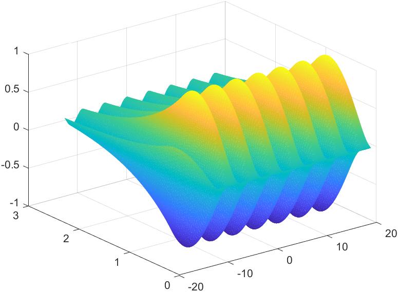
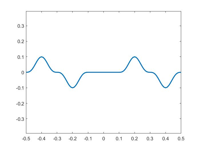
Figure 2. The real part of the mode $\phi^{+}$ (left) and the curve $\Gamma$ (right)

We consider the scattering of the mode $\phi^{+}$ by a local perturbation $q=q(x)$. The total field $u^{tot}=u+\phi^{+}$ as the sum of the incident field $u^{inc}=\phi^{+}$, and the scattered field $u$ satisfies $\Delta u^{tot}+k^{2}(n+q)u^{tot}=0$. Therefore, the scattered field $u$ satisfies $\Delta u+k^{2}(n+q)u=-k^{2}q\,\phi^{+}$ and the radiation condition. In this case the source is given by $f=k^{2}q\,\phi^{+}$. Writing the previous equation as

$$\Delta u+k^{2}nu\ =\ -k^{2}q\,\phi^{+}\ -\ k^{2}q\,u$$

we can – under a smallness assumption on $k^{2}q$ – iterate this fixpoint equation for $u$. The first iteration is the Born approximation $u^{B}$, defined as the solution of $\Delta u^{B}+k^{2}nu^{B}=-k^{2}q\,\phi^{+}$. As a particular example for the perturbation $q$ we choose $q(x_{1},x_{2})=q_{0}\sin^{2}(2\omega x_{1})$ for $(x_{1},x_{2})\in(0,\pi/\omega)\times(0.2,0.7)$ and zero else. Here, $q_{0}>0$ is a parameter. This perturbation has the property that

(39) $$\int\limits_{Q}f(x)\,\overline{\phi^{-}(x)}\,dx = k^{2}\int\limits_{Q}q(x)\,\phi^{+}(x)\,\overline{\phi^{-}(x)}\,dx$$

$$= k^{2}q_{0}\int\limits_{0}^{\pi/\omega}\sin^{2}(2\omega x_{1})\,e^{2i\omega x_{1}}dx_{1}\,\int\limits_{0.2}^{0.7}\sin^{2}(zx_{2})\mathrm{d}x_{2}\ =\ 0\quad\mbox{and}$$

$$\int\limits_{Q}f(x)\,\overline{\phi^{+}(x)}\,dx = k^{2}\int\limits_{Q}q(x)\,|\phi^{+}(x)|^{2}\,dx\ >\ 0\,.$$

From (15) we observe that the Born approximation $u^{B}$ has a right-going mode but no left-going mode.

We choose the parameter $q_{0}=n/2$; that is, the perturbation is (in the $\infty-$norm) of order 50%. For constant $n$ we rewrite the iterative scheme of (6.1) as

$$\frac{a(jh_{y})}{h_{y}^{2}}\bigl{[}v^{(t+1)}_{\ell,\nu,j+1}+v^{(t+1)}_{\ell,\nu,j-1}-2v^{(t+1)}_{\ell,\nu,j}\bigr{]}+\frac{b(jh_{y})}{2h_{y}}\bigl{[}v^{(t+1)}_{\ell,\nu,j+1}-v^{(t+1)}_{\ell,\nu,j-1}\bigr{]}$$

$$+\ [k^{2}n-(\gamma_{\nu}+\ell)^{2}]\,v^{(t+1)}_{\ell,\nu,j}$$

$$= -f_{\ell}\bigl{(}jh_{y},\gamma_{\nu})\ -\ k^{2}\sum_{\mu=0}^{M}w_{\mu}\sum_{m=-L}^{L}q_{\ell-m}(jh_{y},\gamma_{\nu}-\gamma_{\mu})\,v^{(t)}_{m,\mu,j}$$

for $\ell=-L,\ldots,L$ and $j=1,\ldots,n_{y}-1$ and $\nu=0,\ldots,M$, and $t=0,1,\ldots.$. Setting $v^{(0)}_{m,\mu,j}=0$ we obtain $v^{(1)}_{m,\mu,j}$ as the Born approximation. The field $u^{(t)}$ is then computed as the integral

$$u^{(t)}(x_{1},x_{2})\ =\ \sum_{\ell=-L}^{L}\int_{\Gamma}v^{(t)}_{\ell}(x_{2},\alpha)\,e^{i(\ell+\alpha)x_{1}}d\alpha\ \approx\ \sum_{\ell=-L}^{L}\sum_{\mu=0}^{M}v^{(t)}_{\ell}(x_{2},\gamma_{\mu})\,w_{\mu}\,e^{i(\ell+\gamma_{\mu})x_{1}}\,.$$

As a comparison with the PML-method for different parameters $\rho$ we first use the Dirichlet-to-Neumann map as a boundary condition at $x_{2}=h_{0}+\tau$ as explained in Remark 6.1. We computed the relative error $e_{t}:=\|u^{(t+1)}-u^{(t)}\|_{\infty}/\|u^{(t+1)}\|_{\infty}$ on $(-4\pi,6\pi)\times(0,4)$ between consecutive iterates for $t=1,\ldots,8$ as

$$\begin{array}[]{ccccccccc}t:&1&2&3&4&5&6&7&8\\ e_{t}:&0.2276&0.0674&0.0205&0.0048&0.0017&0.0005&0.0001&0.0000\end{array}$$

and show the iterations (real parts) $u^{(1)}$ (i.e. Born), $u^{(2)}$, $u^{(5)}$, and $u^{(9)}$ on $(-4\pi,6\pi)\times(0,4)$ for the Dirichlet-to-Neumann map in Figure 3.

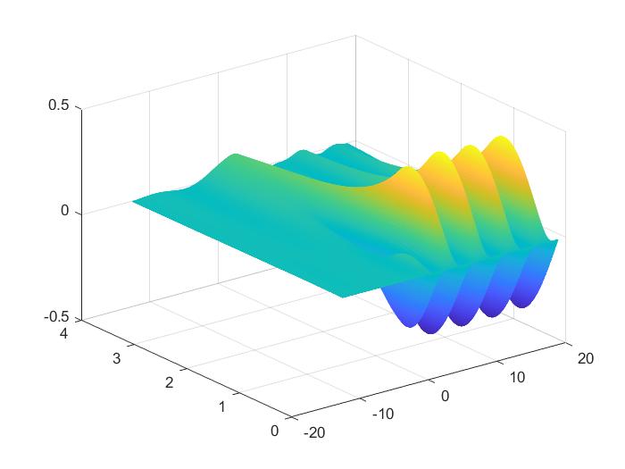
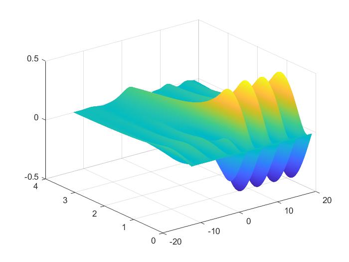
Figure 3. Real parts of $u^{(1)}$ (i.e. Born), $u^{(2)}$, $u^{(5)}$, and $u^{(9)}$.

We clearly observe that the Born approximation; that is, the first iteration, has no left going mode because $f$ is orthogonal to $\phi^{-}$, see (39). The further iterations produce right hand sides which are not orthogonal to $\phi^{-}$ anymore and, therefore, left going modes of small amplitudes appear.

Next, we implemented the PML-method of (6.2) to show the dependence of the result with respect to the parameter $\rho$.. We iterated this system and compared the 4th iteration of the PML-method for parameter $\rho=2,4,6\ldots,20$ with the 4th iteration of the system with Dirichlet-to-Neumann boundary condition. The (semi-logarithmic) plot of the relative errors

$$\max\{|u^{(4)PML}(x)-u^{(4)D2N}(x)|:x\in[-4\pi,6\pi]\times[0,0.9*2.5]\}\ /\ \|u^{(4)D2N}\|_{\infty}$$

of the 4th iterations is shown in Figure 4. One clearly observes the exponential decay.

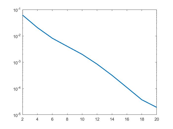
Figure 4. Error as a function of $\rho$ between the 4th iterates of the PML-method and the D2N-boundary condition

Finally, we summarize the settings of the parameters in our simulations:

$$\begin{array}[]{lc}k\mbox{ (wavenumber):}&0.8\\ \omega\mbox{ (propagative wavenumber):}&1.4\\ n\mbox{ (refractive index, determined from $k$ and $\omega$):}&\approx 9.8\\ h_{0}\mbox{ (height of domain without PML-layer):}&2.5\\ \tau\mbox{ (height of PML-layer):}&1.5\\ s_{\rho}\mbox{ (PML-function):}&1+\,\rho\,e^{i\pi/4}(x_{2}-h_{0})^{3}/\tau^{3}\\ n_{y}\mbox{ (number of discretization points in $(0,h_{0}+\tau)$):}&512\\ L\mbox{ (summation bound for spectral representation):}&7\\ M\mbox{ (number of discretization/integration points on $\Gamma$):}&101\\ \end{array}$$

We observed that the results do not depend crucially on the values of $n_{y}$, $L$, or $M$, or the parameters of $s_{\rho}$.

References

[1]
J.-P. Berenger.
A perfectly matched layer for the absorption of electromagnetic
waves.
Journal of Computational Physics, 114(2):185–200, 1994.
[2]
S. N. Chandler-Wilde and P. Monk.
The PML for rough surface scattering.
Applied Numerical Mathematics, 59:2131–2154, 2009.
[3]
Z. Chen and H. Wu.
An adaptive finite element method with perfectly matched absorbing
layers for the wave scattering by periodic structures.
SIAM Journal on Numerical Analysis, 41(3):799–826, 2003.
[4]
J. Coatléven.
Helmholtz equation in periodic media with a line defect.
J. Comp. Phys., 231:1675–1704, 2012.
[5]
D. L. Colton and R. Kress.
Inverse acoustic and electromagnetic scattering theory.
Springer, 4. edition, 2093.
[6]
M. Ehrhardt, H. Han, and C. Zheng.
Numerical simulation of waves in periodic structures.
Commun. Comput. Phys., 5:849–870, 2009.
[7]
M. Ehrhardt, J. Sun, and C. Zheng.
Evaluation of scattering operators for semi-infinite periodic arrays.
Commun. Math. Sci., 7(2):347–364, 2009.
[8]
M. Ehrhardt and C. Zheng.
Exact artificial boundary conditions for problems with periodic
structures.
J. Comput. Phys., 227(14):6877–6894, 2008.
[9]
S. Fliss.
A dirichlet-to-neumann approach for the exact computation of guided
modes in photonic crystal waveguides.
SIAM Journal on Scientific Computing, 35(2):B438–B461, 2013.
[10]
S. Fliss and P. Joly.
Exact boundary conditions for time-harmonic wave propagation in
locally perturbed periodic media.
Appl. Numer. Math., 59:2155–2178, 2009.
[11]
S. Fliss and P. Joly.
Solutions of the time-harmonic wave equation in periodic waveguides:
asymptotic behaviour and radiation condition.
Arch. Rational Mech. Anal., 2015.
[12]
S. Fliss, P. Joly, and V. Lescarret.
A DtN approach to the mathematical and numerical analysis in
waveguides with periodic outlets at infinity.
Pure Appl. Anal., 3(3):487–526, 2021.
[13]
T. Furuya.
Scattering by the local perturbation of an open periodic waveguide in
the half plane.
J. Math. Anal. Appl., 489(1), 2020.
[14]
H. Haddar and T. P. Nguyen.
A volume integral method for solving scattering problems from
locally perturbed infinite periodic layers.
Appl. Anal., 96(1):130–158, 2016.
[15]
V. Hoang.
The limiting absorption principle for a periodic semin-infinite
waveguide.
SIAM J. Appl. Math., 71(3):791–810, 2011.
[16]
T. Hohage and S. Soussi.
Riesz bases and Jordan form of the translation operator in
semi-infinite periodic waveguides.
J. Math. Pures Appl., 100(1):113–135, 2013.
[17]
G. Hu, W. Lu, and A. Rathsfeld.
Time-harmonic acoustic scattering from locally perturbed periodic
curves.
SIAM J. Appl. Math., 81(6):2569–2595, 2021.
[18]
P. Joly, J.-R. Li, and S. Fliss.
Exact boundary conditions for periodic waveguides containing a
local perturbation.
Commun. Comput. Phys., 1:945–973, 2006.
[19]
A. Kirsch.
Scattering by a periodic tube in : part i. the limiting
absorption principle.
Inverse Problems, 35(10):104004, 2019.
[20]
A. Kirsch.
Scattering by a periodic tube in : part i. the
radiation condition.
Inverse Problems, 35(10):104005, 2019.
[21]
A. Kirsch.
A scattering problem for a local perturbation of an open periodic
waveguide.
Math. Methods Appl. Sci., 45(10):5737–5773, 2022.
[22]
A. Kirsch.
On the scattering of a plane wave by a perturbed open periodic
waveguide.
Math. Methods Appl. Sci., 46(9):10698–10718, 2023.
[23]
A. Kirsch and A. Lechleiter.
The limiting absorption principle and a radiation condition for the
scattering by a periodic layer.
SIAM J. Math. Anal., 50(3):2536–2565, 2018.
[24]
A. Kirsch and A. Lechleiter.
A radiation condition arising from the limiting absorption principle
for a closed full‐ or half‐waveguide problem.
Math. Meth. Appl. Sci., 41(10):3955–3975, 2018.
[25]
A. Lechleiter.
The Floquet-Bloch transform and scattering from locally perturbed
periodic surfaces.
J. Math. Anal. Appl., 446(1):605–627, 2017.
[26]
A. Lechleiter and D.-L. Nguyen.
Scattering of Herglotz waves from periodic structures and mapping
properties of the Bloch transform.
Proc. Roy. Soc. Edinburgh Sect. A, 231:1283–1311, 2015.
[27]
A. Lechleiter and R. Zhang.
A convergent numerical scheme for scattering of aperiodic waves from
periodic surfaces based on the Floquet-Bloch transform.
SIAM J. Numer. Anal, 55(2):713–736, 2017.
[28]
A. Lechleiter and R. Zhang.
A Floquet-Bloch transform based numerical method for scattering
from locally perturbed periodic surfaces.
SIAM J. Sci. Comput., 39(5):B819–B839, 2017.
[29]
X. Yu, G. Hu, W. Lu, and A. Rathsfeld.
PML and high-accuracy boundary integral equation solver for
wave scattering by a locally defected periodic surface.
SIAM J. Numer. Anal., 60(5):2592–2625, 2022.
[30]
L. Yuan and Y. Y. Lu.
A recursive doubling Dirichlet-to-Neumann map method for periodic
waveguides.
J. Lightwave technol., 25:3649–3656, 2007.
[31]
R. Zhang.
A high order numerical method for scattering from locally perturbed
periodic surfaces.
SIAM J. Sci. Comput., 40(4):A2286–A2314, 2018.
[32]
R. Zhang.
Numerical method for scattering problems in periodic waveguides.
Numer. Math., 148:959–996, 2021.
[33]
R. Zhang.
Spectrum decomposition of translation operators in periodic
waveguide.
SIAM Journal on Applied Mathematics, 81(1):233–257, 2021.
[34]
R. Zhang.
Exponential convergence of perfectly matched layers for scattering
problems with periodic surfaces.
SIAM J. Numer. Math., 60(2):804–823, 2022.
[35]
R. Zhang.
High order complex contour discretization methods to simulate
scattering problems in locally perturbed periodic waveguides.
SIAM J. Sci. Comput., 44(5):B1257–B1281, 2022.
[36]
R. Zhang.
Higher-order convergence of perfectly matched layers in
three-dimensional biperiodic surface scattering problems.
SIAM J. Numer. Anal., 61(6):2917–2939, 2023.