Revisiting Nonlocal Self-Similarity from Continuous Representation

Abstract

Nonlocal self-similarity (NSS) is an important prior that has been successfully applied in multi-dimensional data processing tasks, e.g., image and video recovery. However, existing NSS-based methods are solely suitable for meshgrid data such as images and videos, but are not suitable for emerging off-meshgrid data, e.g., point cloud and climate data. In this work, we revisit the NSS from the continuous representation perspective and propose a novel Continuous Representation-based NonLocal method (termed as CRNL), which has two innovative features as compared with classical nonlocal methods. First, based on the continuous representation, our CRNL unifies the measure of self-similarity for on-meshgrid and off-meshgrid data and thus is naturally suitable for both of them. Second, the nonlocal continuous groups can be more compactly and efficiently represented by the coupled low-rank function factorization, which simultaneously exploits the similarity within each group and across different groups, while classical nonlocal methods neglect the similarity across groups. This elaborately designed coupled mechanism allows our method to enjoy favorable performance over conventional NSS methods in terms of both effectiveness and efficiency. Extensive multi-dimensional data processing experiments on-meshgrid (e.g., image inpainting and image denoising) and off-meshgrid (e.g., climate data prediction and point cloud recovery) validate the versatility, effectiveness, and efficiency of our CRNL as compared with state-of-the-art methods.

I Introduction

TABLE I: Comparisons of classical nonlocal methods and our new continuous representation-based nonlocal method in terms of applicabilities and encoded priors.

		BM3D[1]	NLR-CS[2]	WNNM[3]	WNLRATV[4]	NL-FCTN[5]	CRNL
Applicabilities	Meshgrid data	✓	✓	✓	✓	✓	✓
	Off-meshgrid data						✓
Priors	Similarity within a group	✓	✓	✓	✓	✓	✓
	Similarity across groups						✓

With the rapid development of imaging and sensing technologies, numerous types of multi-dimensional data are readily available. Among them, signals with meshgrid structures can be conventionally modeled as arrays with one or multiple dimensions, e.g., a gray image can be represented by a matrix and a color image can be represented by a third-order tensor. Digging their intrinsic structures via hand-crafted techniques is an effective approach for many signal processing tasks. For example, real-world data usually has internal low-dimensional structures, and thus low-rank representation is a popular technique for data analysis and processing, e.g., inpainting [6], denoising [7], and compressed sensing [8]. Besides, many data have intense local smoothness, which can be finely characterized by smooth regularizations such as total variation [9, 10] and smooth factorization [11, 12].

One of the mostly employed prior structures of real-world data is the nonlocal self-similarity (NSS). The NSS refers to the fact that a signal often contains many repetitive local patterns, and thus a local pattern always has many similar patterns across the whole signal [13, 14]. The NSS of data has been widely used in different multi-dimensional processing tasks, e.g., image restoration [13, 15, 3], hyperspectral denoising [16, 17], compressed sensing [18, 19], and tensor completion [20].

The conventional approach of these NSS-based methods is to search similar patches and then group these patches into a new matrix/tensor, followed by low-rank or/and smooth regularizations performed on the constructed matrix/tensor to effectively reconstruct the original signal[4, 21, 22]. Such strategy utilizes the nonlocal information and is usually more effective than directly performing low-rank/smooth regularizations in the original domain [23, 24], since the similar patch groups are expected to enjoy more evident low-rank/smooth structures. Currently, NSS has also been integrated into many deep learning frameworks [25, 26, 27], showing certain advantages over traditional neural networks due to the beneficial nonlocal information.

Although these NSS-based methods have made great success in multiple areas, they are solely suitable to exploiting the NSS of meshgrid data, such as images. However, many emerging real-world data are not arranged as aligned arrays, but rather placed in unordered off-meshgrid positions in the space, e.g., point cloud and climate data. In order to exploit the underlying NSS of such off-meshgrid data, it is needed to develop a new fundamental nonlocal method that is suitable for both on-meshgrid and off-meshgrid data.

To meet this challenge, we revisit the NSS from the continuous representation perspective and propose a novel Continuous Representation-based NonLocal method (termed as CRNL), which can exploit the NSS of both on-meshgrid and off-meshgrid data under a unified framework. Concretely, we first use implicit neural representation (INR) to learn a continuous representation of observed discrete data. Then, we divide the continuous space into basic continuous cubes. We measure the similarity between continuous cubes, instead of discrete patches, using the learned continuous representation and stack similar cubes into a continuous group. To compactly and efficiently represent nonlocal continuous groups, we propose the coupled low-rank function factorization, where the shared factor functions exploit the similarity across different groups, and the unshared core tensors respect the individuality of each group. The compact coupled factorization allows our method to enjoy advantageous performance in terms of both effectiveness and computational efficiency. A general illustration of our CRNL is illustrated in Fig. 1.

Compared to classical NSS-based methods, the essential advantages of our CRNL are contained in two folds. First, based on the continuous representation, our CRNL can measure the self-similarity of both on-meshgrid and off-meshgrid data. It is thus expected to be more versatile than conventional NSS-based methods, which are solely suitable for meshgrid data. Second, the nonlocal continuous groups are compactly and efficiently represented by the coupled low-rank function factorization, which simultaneously exploits the similarity within each group and across different groups; see Lemma 3. As compared, classical NSS-based methods employ independent uncoupled representations for different groups, which neglects the similarity across groups. Such compact coupled factorization manner makes our method not only able to enjoy favorable computational efficiency with elaborate parameters sharing across different NSS groups, but also hopefully enhance the performance of multi-dimensional data recovery through essential correlation knowledge existed across different groups.

In summary, this paper makes the following contributions:

• We revisit the NSS from the continuous representation perspective and propose the CRNL, which can measure the self-similarity of both on-meshgrid and off-meshgrid data through the continuous representation. As compared with classical nonlocal methods, our CRNL is more versatile for real-world multi-dimensional data processing on and off-meshgrid.

• We propose the coupled low-rank function factorization to represent nonlocal continuous groups, which simultaneously exploits the similarity within each group and across different groups to more comprehensively modeling the underlying structures of multi-dimensional data. The elaborately designed coupled mechanism allows our method to enjoy advantageous computational efficiency as compared with classical nonlocal methods.

• To demonstrate the effectiveness of our method, we conduct experiments on multiple data recovery tasks including image inpainting, denoising (on-meshgrid data), and multivariate regression problems (off-meshgrid data, e.g., climate data and point clouds). Extensive results demonstrate the effectiveness of our method as compared with state-of-the-art methods.

The rest of this paper is organized as follows. In Sec. II, we introduce related work. In Sec. III, we present the proposed method. In Sec. IV, we carry out experiments on different tasks and make some discussions on the proposed method. Sec. V concludes this paper.

II Related Work

II-A Nonlocal Self-Similarity-Based Methods

The NSS-based methods have been widely studied in the literature. The pioneer works, e.g., [28] and [1], considered nonlocal means or nonlocal filters for image recovery. Later works mostly considered nonlocal sparse/low-rank regularizations for image recovery, e.g., by using the weighted nuclear norm [3] or groups sparsity [29] performed on nonlocal patch groups. Recently, many nonlocal low-rank-based methods were proposed in different areas, such as compressive sensing [2, 8], hyperspectral image restoration [16, 4], video deraining [23], magnetic resonance imaging [24], and seismic data processing [30]. These wide applications have demonstrated the effectiveness of NSS-based methods. As compared, our method has two innovative features that are significantly different from existing NSS-based methods. First, existing NSS-based methods are solely suitable for meshgrid data processing[13, 15, 3], while our method learns a continuous representation of the observed discrete data, and hence is suitable for both on-meshgrid and off-meshgrid data. Second, existing NSS-based methods use classical low-rank regularization such as weighted nuclear norm [3] and low-rank tensor factorization [31] to reconstruct nonlocal patch groups, while our method leverages the coupled low-rank function factorization defined in a continuous domain to represent continuous groups. The compact coupled factorization significantly reduces computational costs and simultaneously characterizes both the intra- and inter-group similarity, which helps to better recover the underlying data.

Recently, Chen et al. [32] and Zhu et al. [33] have proposed nonlocal methods for point cloud recovery, which mainly design feature descriptors to encode the information of points as patch matrix, and then perform nonlocal low-rank matrix recovery to recover the noisy matrix of point cloud. These methods cleverly transform the point cloud processing task into matrix recovery. However, these methods were specifically designed for point clouds, while our method is a unified method that can be applied to both on-meshgrid and off-meshgrid data representation, e.g., images and point clouds.

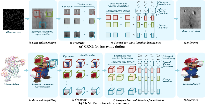
Figure 1: The overall flowchart of our continuous representation-based nonlocal method for data recovery. Here, we take the image inpainting and point cloud recovery as examlpes.

II-B Basis Function-Based Methods

In our CRNL, we propose the coupled low-rank function factorization to parameterize the nonlocal continuous groups for continuous representation. In the literature, some low-rank matrix/tensor methods also employ basis functions to parameterize the low-rank model, which is related to our method. The pioneer works [11, 12] considered using Gaussian basis or polynomial basis to parameterize the factor matrix in low-rank matrix factorization, which induces some implicit smoothness over the resultant matrix. The implicit smoothness was further introduced into higher-order low-Tucker-rank [34] and low-CP-rank tensor models [35] by using the Fourier basis. Oseledets [36] introduced explicit representations of some multivariate functions (e.g., the polynomial and sine functions) in tensor-train factorization format. Hashemi and Trefethen [37] studied Tucker factorization of functions and proposed algorithms for approximating functions in Tucker format, where the factor functions are represented by Chebyshev expansions. The main differences between our method and these works are three folds. First, our method additionally exploits the nonlocal information of data to more accurately capture the implicit low-rank structures. Second, our method can be applied to both on-meshgrid and off-meshgrid data processing, while previous basis function-based low-rank methods are hard to be directly applied to data processing tasks beyond meshgrid. Third, we employ the implicit deep neural network [38] as basis functions to parameterize the coupled low-rank function factorization, while previous methods use shallow basis functions, and thus our method is expected to hold stronger representation abilities.

II-C Continuous Representation-Based Methods

The continuous representation is a powerful tool for data representation on and off-meshgrid. The most popular method of continuous representation is the implicit neural representation, or INR [38, 39]. The core idea of INR is to use a neural network that maps coordinates to the corresponding value for data representation. It is a powerful tool for representing various signals like images [40], shapes [41], and point clouds [42]. INR has also shown promising performances for data recovery tasks. For example, Chen et al. [43] proposed the local implicit image function for image super-resolution. It was further enhanced by introducing details recovery technique [40] and advanced deep network [44]. Zhang et al. [45] proposed to use INR for hyperspectral image super-resolution. However, these methods are supervised methods that need supervised training process, while our CRNL is a hand-crafted unsupervised method, which learns the continuous representation directly from observed data. Another type of INR is the unsupervised one, e.g., Zhao et al. [42] utilized the INR for self-supervised point cloud upsampling, and Kim et al. [46] proposed to use INR for zero-shot image recovery. As compared with these two unsupervised data recovery methods using INR, our CRNL additionally leverages the nonlocal low-rankness to capture internal low-dimensional structures of data, which is helpful to increase the effectiveness and generalization abilities of the continuous representation.

III The Proposed Method

III-A Preliminaries

Scalars, vectors, matrices, and tensors are denoted by $x$, $\bf x$, $\bf X$, and $\mathcal{X}$, respectively. The $i$-th element of $\bf x$ is denoted by ${\bf x}_{(i)}$, and it is similar for matrices and tensors, i.e., ${\bf X}_{(i_{1},i_{2})}$ and ${\mathcal{X}}_{(i_{1},i_{2}\cdots,i_{N})}$. When we use the index $:$, e.g., ${\bf X}_{(i,:)}$, it represents the $i$-th row of $\bf X$. The tensor Frobenius norm of a $N$-th-order tensor ${\mathcal{X}}\in{\mathbb{R}}^{n_{1}\times\cdots\times n_{N}}$ is defined as $\left\lVert{\mathcal{X}}\right\rVert_{F}:=\sqrt{\langle{\mathcal{X}},{\mathcal{X}}\rangle}=\sqrt{\sum_{i_{1},\cdots,i_{N}}{\mathcal{X}}_{(i_{1},\cdots,i_{N})}^{2}}$. The tensor $\ell_{1}$-norm is defined as $\left\lVert{\mathcal{X}}\right\rVert_{\ell_{1}}:=\sum_{i_{1},\cdots,i_{N}}|{\mathcal{X}}_{(i_{1},\cdots,i_{N})}|$. The unfolding operator of a tensor ${\mathcal{X}}\in{\mathbb{R}}^{n_{1}\times\cdots\times n_{N}}$ along the $d$-th mode ($d=1,2,\cdots,N$) is defined as ${\tt unfold}_{d}(\cdot):{\mathbb{R}}^{n_{1}\times\cdots\times n_{N}}\rightarrow{\mathbb{R}}^{n_{d}\times\prod_{j\neq d}n_{j}}$, which returns the unfolding matrix along the mode $d$, and the unfolding matrix is denoted by ${\bf X}^{(d)}:={\tt unfold}_{d}({\mathcal{X}})$. ${\tt fold}_{d}(\cdot)$ denotes the inverse operator of ${\tt unfold}_{d}(\cdot)$. The mode-$d$ ($d=1,2,\cdots,N$) tensor-matrix product is defined as ${\mathcal{X}}\times_{d}{\bf A}:={\tt fold}_{d}({\bf A}{\bf X}^{(d)})$, which returns a tensor.

Lemma 1.

(Tensor Tucker factorization [47]) The Tucker rank of a $N$-th-order tensor ${\mathcal{X}}\in{\mathbb{R}}^{n_{1}\times\cdots\times n_{N}}$ is a vector defined as ${\rm rank}_{T}({\mathcal{X}}):=({\rm rank}({\bf X}^{(1)}),{\rm rank}({\bf X}^{(2)}),\cdots,{\rm rank}({\bf X}^{(N)}))$.

• If ${\rm rank}_{T}({\mathcal{X}})=(r_{1},r_{2},\cdots,r_{N})$, then there exist a core tensor ${\mathcal{C}}\in{\mathbb{R}}^{r_{1}\times r_{2}\times\cdots\times r_{N}}$ and $N$ factor matrices ${\bf U}_{d}\in{\mathbb{R}}^{n_{d}\times r_{d}}$ ($d=1,2,\cdots,N$) such that ${\mathcal{X}}={\mathcal{C}}\times_{1}{\bf U}_{1}\times_{2}{\bf U}_{2}\times_{3}\cdots\times_{N}{\bf U}_{N}$.

• Let ${\mathcal{C}}\in{\mathbb{R}}^{r_{1}\times\cdots\times r_{N}}$ be an arbitrary $N$-th-order tensor, ${\bf U}_{d}\in{\mathbb{R}}^{n_{d}\times r_{d}}$ ($d=1,2,\cdots,N$) be arbitrary matrices ($r_{d}\leq n_{d}$). Then $\big{(}{\rm rank}_{T}({\mathcal{C}}\times_{1}{\bf U}_{1}\times_{2}{\bf U}_{2}\times_{3}\cdots\times_{N}{\bf U}_{N})\big{)}_{(d)}\leq r_{d}$ ($d=1,2,\cdots,N$).

TABLE II: Notations used in this section.

Notation	Description
$N$	The number of dimensions of the observed data
$h(\cdot)$	The observed multivariate function
$D_{h}\subset{\mathbb{R}}^{N}$	The set of observed coordinates
${D_{h}}^{C}\subset{\mathbb{R}}^{N}$	The set of unobserved coordinates (testing set)
$f_{\theta}(\cdot)$	The continuous representation of the observed data
$D_{f_{\theta}}\subset{\mathbb{R}}^{N}$	The entire continuous domain
$[a_{d},b_{d}]\subset{\mathbb{R}}$	The continuous domain in the $d$-th dimension ($d=1,\cdots,N$)
$n_{d}$	The number of basic units in the $d$-th dimension
$\delta_{d}\in{\mathbb{R}}$	The basic unit length in the $d$-th dimension
$p\delta_{d}$	The basic cube length in the $d$-th dimension ($p$ is an integer)
$D_{t}\subset{\mathbb{R}}^{N}$	The $t$-th overlapped basic continuous cube ($t=1,\cdots,T$)
$D_{l}^{\rm key}\subset{\mathbb{R}}^{N}$	The $l$-th non-overlapping key continuous cube ($l=1,\cdots,L$)
$D_{l_{s}}\subset{\mathbb{R}}^{N}$	The $s$-th similar cube of the $l$-th key cube ($s=1,\cdots,S$)
${\hat{D}}_{h_{l}}\subset{\mathbb{R}}^{N+1}$	The set of observed points of the $l$-th continuous group

III-B Overview of the Proposed CRNL

Classical NSS-based methods are suitable for meshgrid data processing, e.g., image inpainting, but are not suitable for off-meshgrid data processing, e.g., point cloud processing. To address this limitation, we revisit the NSS from the continuous representation perspective and propose the CRNL for data processing on and off-meshgrid. Specifically, we view the observed data as a real function $h(\cdot):{\mathbb{R}}^{N}\rightarrow{\mathbb{R}}$, where $N$ denotes the number of dimensions of the observed data (e.g., for a color image, $N=3$ corresponds to height, width, and channels). Suppose that we are given some discrete observations of $h(\cdot)$, i.e., we have a coordinate set with limited number of coordinate points ${D_{h}}\subset{\mathbb{R}}^{N}$ and the corresponding observed function values $h({\bf v}),{\bf v}\in{D_{h}}$. The goal is often to infer the function values of $h(\cdot)$ at unobserved positions in ${D_{h}}^{C}$, where ${D_{h}}^{C}$ denotes the complementary set of ${D_{h}}$, i.e., the unobserved coordinates in the whole set. Typical examples include image inpainting and multivariate regression problems, where $D_{h}$ is located in meshgrid and non-meshgrid coordinate locations, respectively.

To more clearly introduce our method, we first give a rough description in this subsection, and then illustrate the detailed algorithms step by step. In general, our method includes the following steps for multi-dimensional data processing:

• Basic cubes splitting We first use INR to learn a continuous representation of the observed discrete data. Based on the continuous representation, we split the continuous space into basic continuous cubes.

• Grouping We use the continuous representation to measure the similarity between basic continuous cubes. We stack similar continuous cubes into a continuous group. Each continuous group contain a certain number of observed points; see Fig. 2.

• Coupled low-rank function factorization We propose the coupled low-rank function factorization to compactly represent continuous groups, where the shared factor functions characterize the similarity across groups, and the unshared core tensors reveal the individuality of each group. The coupled function factorization allows our method to enjoy favorable computational efficiency for representing numerous number of continuous groups.

As compared with classical discrete representation-based NSS methods, the essential differences of our CRNL are in two folds. First, we use the INR to learn a continuous representation of data and split the continuous space into basic continuous cubes, which naturally allows us to handle data on and off-meshgrid. Second, different from classical NSS methods that adopt discrete and separate low-rank representation for each nonlocal patch group, our CRNL leverages the coupled low-rank function factorization defined in a continuous space to more compactly and accurately represent all nonlocal groups in a parameters sharing manner through globally extracting correlation knowledge among them. An overview of our proposed CRNL for multi-dimensional data recovery is illustrated in Fig. 1.

III-C Detailed Algorithm of CRNL

1) Basic cubes splitting Given the observed function $h(\cdot):{\mathbb{R}}^{N}\rightarrow{\mathbb{R}}$ with observed discrete coordinate set ${D_{h}}\subset{\mathbb{R}}^{N}$, we first use the INR [38] to learn a continuous representation of the observed data. Specifically, we use an explicit form of neural network $f_{\theta}(\cdot):{\mathbb{R}}^{N}\rightarrow{\mathbb{R}}$ to approximate the observed function $h(\cdot)$ over the observed discrete set ${D_{h}}$:

$$\begin{split}&\min_{\theta}\sum_{{\bf v}\in{D_{h}}}(h({\bf v})-f_{\theta}({\bf v}))^{2}+\psi[f_{\theta}(\cdot)],\end{split}$$ (1)

where $\theta$ denote the learnable parameters of the neural network $f_{\theta}(\cdot)$ and $\psi[f_{\theta}(\cdot)]$ denotes a regularization term that enhances the performance (The regularization term is conditioned on tasks, specified in Sec. III-E). We use the Adam optimizer[48] to optimize the INR model (1).

Next, we conduct basic cubes splitting. For easy reference, a notation table is provided in Table II. The basic cubes splitting includes the following steps:

Figure 2: Illustrations of the proposed basic cubes splitting and grouping process in the three-dimensional case ($N=3$) with number of units $n_{1}=n_{2}=5$ and cube size $p=2$. Here, $D_{t}$ denotes the basic continuous cube, $D_{l}^{\rm key}$ denotes a key continuous cube, and $D_{l_{1}},D_{l_{2}}$ denote the two extracted similar continuous cubes of the $l$-th key cube $D_{l}^{\rm key}$.

• First, the observed coordinate set $D_{h}\subset{\mathbb{R}}^{N}$ contains $N$ dimensions (e.g., $N=2$ for a gray image and $N=3$ for a color image). For the $d$-th dimension ($d=1,\cdots,N$), we denote the minimal value of the observed data coordinates as $a_{d}:=\min_{{\bf v}\in D_{h}}{\bf v}_{(d)}$, where ${\bf v}_{(d)}$ denotes the $d$-th element of the vector ${\bf v}$. Similarly we denote the maximum value of the observed data coordinates in the $d$-th dimension as $b_{d}:=\max_{{\bf v}\in D_{h}}{\bf v}_{(d)}$. The continuous domain underlying the observed data in the $d$-th dimension is $[a_{d},b_{d}]\subset{\mathbb{R}}$ ($d=1,\cdots,N$). Based on the continuous domain of each dimension, the entire $N$-dimensional continuous domain $D_{f_{\theta}}\subset{\mathbb{R}}^{N}$ is a cubic space $D_{f_{\theta}}:=[a_{1},b_{1}]\times[a_{2},b_{2}]\times\cdots\times[a_{N},b_{N}]\subset{\mathbb{R}}^{N}$.

• Second, we split the continuous space $D_{f_{\theta}}$ into small basic continuous units. Specifically, we split the first dimension of $D_{f_{\theta}}$, i.e., $[a_{1},b_{1}]$, into $n_{1}$ non-overlapping regions $[a_{1},a_{1}+\delta_{1}),[a_{1}+\delta_{1},a_{1}+2\delta_{1}),\cdots,[a_{1}+(n_{1}-1)\delta_{1},a_{1}+n_{1}\delta_{1})$, where $\delta_{1}$ denotes the interval in the first dimension such that $a_{1}+n_{1}\delta_{1}=b_{1}$. Similarly, we split the second dimension $[a_{2},b_{2}]$ into $n_{2}$ non-overlapping regions, i.e., $[a_{2},a_{2}+\delta_{2}),[a_{2}+\delta_{2},a_{2}+2\delta_{2}),\cdots,[a_{2}+(n_{2}-1)\delta_{2},a_{2}+n_{2}\delta_{2})$, where $a_{2}+n_{2}\delta_{2}=b_{2}$. Such split leads to a finite disjoint coverage over $D_{f_{\theta}}$ with $n_{1}n_{2}$ units, where each unit has the volume of $\delta_{1}\times\delta_{2}\times(b_{3}-a_{3})\times\cdots\times(b_{N}-a_{N})$.

• Third, we construct basic continuous cubes. A continuous cube is composed of $p^{2}$ basic units, where $p$ determines the cube size. We first construct overlapped basic continuous cubes with volume $p\delta_{1}\times p\delta_{2}\times(b_{3}-a_{3})\times\cdots\times(b_{N}-a_{N})$ and stride 1 along the first and second dimensions. It results in a continuous cubes set $\{D_{t}\subset{\mathbb{R}}^{N}\}_{t=1}^{T}$ that contains $T=(n_{1}-p+1)(n_{2}-p+1)$ basic continuous cubes. Similarly, we construct non-overlapping key continuous cubes with the same cube size but with stride $p$, which results in a key continuous cubes set $\{D_{l}^{\rm key}\subset{\mathbb{R}}^{N}\}_{l=1}^{L}$ that contains $L=(n_{1}/p)(n_{2}/p)$ key cubes.

Fig. 2 illustrates a basic cubes splitting process with $n_{1}=n_{2}=5$ and $p=2$.

2) Grouping Next, we use the learned continuous representation $f_{\theta}(\cdot)$ to measure the similarity between basic continuous cubes. Specifically, for each non-overlapping key continuous cube $D_{l}^{\rm key}$, we aim to find its top-$S$ similar continuous cubes in the overlapped candidate cubes set $\{D_{t}\}_{t=1}^{T}$. The distance between two continuous cubes $D_{l}^{\rm key}$ and $D_{t}$ is calculated by the Euclidean distance between function values of $f_{\theta}(\cdot)$ at corresponding meshgrid positions in these two cubes, i.e., the sum of $(f_{\theta}({\bf v}^{\rm key})-f_{\theta}({\bf v}))^{2}$, where ${\bf v}^{\rm key}$ and ${\bf v}$ are one-to-one corresponding meshgrid coordinate points in $D_{l}^{\rm key}$ and $D_{t}$. For each key cube $D_{l}^{\rm key}$, we measure its similarity with each candidate cube in $\{D_{t}\}_{t=1}^{T}$ using this distance metric and stack the top-$S$ similar cubes into a continuous group $\{D_{l_{s}}\}_{s=1}^{S}$. Fig. 2 gives an intuitive illustration.

A continuous group $\{D_{l_{s}}\}_{s=1}^{S}$ is then composed of $S$ similar cubes. The coordinate values in different cubes are not within the same area, which bring difficulty for the subsequent continuous group representation. Hence, for each continuous cubes group $\{D_{l_{s}}\}_{s=1}^{S}$, we gather all observed points in different cubes into the same area to construct a new observed points set. Specifically, for any $s\in\{1,2,\cdots,S\}$, we modify the values of the observed points in $D_{l_{s}}$ such that the new observed points fall into the key cube space $D_{l}^{\rm key}$. Formally, we denote the spatial distance (say $\Delta x$ and $\Delta y$) between the key cube $D_{l}^{\rm key}$ and the similar cube $D_{l_{s}}$ as

$$\begin{split}&\Delta x=\min_{{\bf u}\in D_{l}^{\rm key}}{\bf u}_{(1)}-\min_{{\bf u}\in D_{l_{s}}}{\bf u}_{(1)},\\ &\Delta y=\min_{{\bf u}\in D_{l}^{\rm key}}{\bf u}_{(2)}-\min_{{\bf u}\in D_{l_{s}}}{\bf u}_{(2)}.\end{split}$$ (2)

Then, for any observed point ${\bf v}\in D_{l_{s}}\cap D_{h}$, where $D_{l_{s}}\cap D_{h}$ denotes the set of observed points in the continuous cube $D_{l_{s}}$, we modify its values to construct a new vector:

$$\begin{split}\Big{(}{\bf v}_{(1)}+\Delta x,{\bf v}_{(2)}+\Delta y,{\bf v}_{(3)},\cdots,{\bf v}_{(N)}\Big{)}\in D_{l}^{\rm key}.\end{split}$$ (3)

This new vector belongs to the key cube space $D_{l}^{\rm key}$. By further catenating this new vector with its cube index $s$, we obtain a new observed point

$$\begin{split}{\bf w}_{{\bf v},s}:=\Big{(}{\bf v}_{(1)}+\Delta x,{\bf v}_{(2)}+\Delta y,{\bf v}_{(3)},\cdots,{\bf v}_{(N)},s\Big{)}\in{\mathbb{R}}^{N+1},\end{split}$$

which is conditioned on the original observed point $\bf v$ and the similar cube index $s$. We cluster all such points in the $l$-th continuous group $\{D_{l_{s}}\}_{s=1}^{S}$ to obtain a new observed dataset

$${\hat{D}}_{h_{l}}=\bigcup_{s\in\{1,2,\cdots,S\}}\bigcup_{{\bf v}\in{D}_{l_{s}}\cap{D_{h}}}\{{\bf w}_{{\bf v},s}\}\subset{\mathbb{R}}^{N+1}.$$ (4)

The new observed set ${\hat{D}}_{h_{l}}\subset{\mathbb{R}}^{N+1}$ contains all observed points in the $l$-th continuous group. The corresponding observed $(N+1)$-dimensional function $h_{l}(\cdot):\Omega\rightarrow{\mathbb{R}}$ ($l=1,2,\cdots,L$), where ${\hat{D}}_{h_{l}}\subset\Omega\subset{\mathbb{R}}^{N+1}$, map the observed points in ${\hat{D}}_{h_{l}}$ to the corresponding values, in which each multivariate function $h_{l}(\cdot)$ corresponds to a continuous group $\{D_{l_{s}}\}_{s=1}^{S}$.

3) Coupled low-rank function factorization Inspired by many conventional strategies to represent NSS patch group by low-rank structures [3, 31], we also use the low-rank representation to represent each continuous group. Here, the observed points in ${\hat{D}}_{h_{l}}$ may be off-meshgrid, and thus standard discrete low-rank tensor representation is incapable of dealing with the off-meshgrid observations. Instead, our proposed coupled low-rank function factorization defined in a continuous domain can easily handle this issue.

The core idea of low-rank function representation is to use a core tensor $\cal C$ and $N+1$ factor functions $f_{\theta_{1}}(\cdot),\cdots,f_{\theta_{N+1}}(\cdot)$ to represent the original ($N+1$)-dimensional function $h_{l}(\cdot)$ through the low-rank tensor function factorization [49]. Theoretically, a multivariate function with low-rank structures can be exactly factorized into a core tensor and some factor functions. On the other hand, the product between a core tensor and some factor functions forms a multivariate function with low-rankness, as stated below.

Lemma 2.

(Low-rank tensor function factorization) Let $h_{l}(\cdot):\Omega\rightarrow{\mathbb{R}}$ be a bounded multivariate function, where $\Omega=\Omega_{1}\times\Omega_{2}\times\cdots\times\Omega_{N+1}\subset{\mathbb{R}}^{N+1}$ is the definition domain. Define the “function rank (F-rank)” of $h_{l}(\cdot)$ as the maximum Tucker rank of tensors that can be sampled on the multivariate function $h_{l}(\cdot)$ with meshgrid partitions [49]. Then:

• (Existence of low-rank tensor function factorization) If ${\rm F\text{-}rank}[h_{l}]=(r_{1},r_{2},\cdots,r_{N+1})$, then there exist a core tensor ${\mathcal{C}}\in{\mathbb{R}}^{r_{1}\times r_{2}\times\cdots\times r_{N+1}}$ and $N+1$ bounded factor functions $f_{1}(\cdot):\Omega_{1}\rightarrow{\mathbb{R}}^{r_{1}}$, $f_{2}(\cdot):\Omega_{2}\rightarrow{\mathbb{R}}^{r_{2}}$,$\cdots$, $f_{N+1}(\cdot):\Omega_{N+1}\rightarrow{\mathbb{R}}^{r_{N+1}}$ such that for any ${\bf v}\in\Omega$, $h_{l}({\bf v})={\mathcal{C}}\times_{1}f_{1}({\bf v}_{(1)})\times_{2}f_{2}({\bf v}_{(2)})\times_{3}\cdots\times_{N+1}f_{N+1}({\bf v}_{(N+1)})$.

• (Low-rankness guarantee of the tensor function factorization) Let ${\mathcal{C}}\in{\mathbb{R}}^{r_{1}\times r_{2}\times\cdots\times r_{N+1}}$ be an arbitrary tensor and $f_{1}(\cdot):\Omega_{1}\rightarrow{\mathbb{R}}^{r_{1}}$, $f_{2}(\cdot):\Omega_{2}\rightarrow{\mathbb{R}}^{r_{2}}$,$\cdots$, $f_{N+1}(\cdot):\Omega_{N+1}\rightarrow{\mathbb{R}}^{r_{N+1}}$ be $N+1$ arbitrary bounded factor functions. Then we have $({\rm F\text{-}rank}[h_{l}])_{(d)}\leq r_{d}$ ($d=1,2,\cdots,N+1$), where $h_{l}(\cdot):\Omega=\Omega_{1}\times\Omega_{2}\times\cdots\times\Omega_{N+1}\rightarrow{\mathbb{R}}$ is defined by $h_{l}({\bf v})={\mathcal{C}}\times_{1}f_{1}({\bf v}_{(1)})\times_{2}f_{2}({\bf v}_{(2)})\times_{3}\cdots\times_{N+1}f_{N+1}({\bf v}_{(N+1)})$ for any ${\bf v}\in\Omega$.

Lemma 2 indicates that the low-rank function factorization can compactly represent a multivariate function in the low-rank format, and hence is suitable to represent the low-rank continuous group. Directly applying the low-rank function factorization to represent each group leads to large computational costs due to the numerous number of continuous groups. Specifically, it needs $L$ core tensors and $L\times(N+1)$ factor functions to represent $L$ continuous groups by using the low-rank function representation, which is quite computationally expensive. Meanwhile, similar to classical NSS-based methods [50, 4, 5], such uncoupled independent representations of nonlocal groups neglect the similarity across different groups, and hence is insufficient to accurately model the underlying structures of nonlocal groups.

To address the above issues, we propose the coupled low-rank function factorization, which employs $N+1$ factor functions shared by all continuous groups. Specifically, we employ $L$ low-rank tensor functions $\{s_{l}(\cdot)\}_{l=1}^{L}$ parameterized by different core tensors ${\mathcal{C}}_{l}\in{\mathbb{R}}^{r_{1}\times r_{2}\times r_{3}\times\cdots\times r_{N+1}}$ ($l=1,2,\cdots,L$) but share the same $N+1$ factor functions $\{f_{\theta_{d}}(\cdot)\}_{d=1}^{N+1}$ to represent the continuous groups in the low-rank format. The coupled low-rank function factorization solely uses $L$ core tensors and $N+1$ factor functions to represent $L$ continuous groups, which inclines to largely reduce computational costs. Meanwhile, the coupled mechanism simultaneously exploits the similarity within each group and across different groups, which is expected to more faithfully take advantage of the intrinsic correlation knowledge across different local areas of multi-dimensional data (see Sec. III-D for detailed analysis).

Formally, we propose the following coupled low-rank function factorization-based model to compactly represent continuous groups $\{h_{l}(\cdot)\}_{l=1}^{L}$:

$$\begin{split}&\min_{\{{\mathcal{C}}_{l}\}_{l=1}^{L},\{\theta_{d}\}_{d=1}^{N+1}}\sum_{l=1}^{L}\Big{(}\sum_{{\bf v}\in{\hat{D}}_{h_{l}}}(h_{l}({\bf v})-s_{l}({\bf v}))^{2}+\psi[s_{l}(\cdot)]\;\Big{)},\;\\ &s_{l}({\bf v}):={\mathcal{C}}_{l}\times_{1}f_{\theta_{1}}({\bf v}_{(1)})\times_{2}\cdots\times_{N+1}f_{\theta_{N+1}}({\bf v}_{(N+1)}),\end{split}$$ (5)

where $h_{l}(\cdot)$ is the observed function of the $l$-th continuous group, $s_{l}(\cdot):{\mathbb{R}}^{N+1}\rightarrow{\mathbb{R}}$ ($l=1,2,\cdots,L$) denotes the desired recovered low-rank function of the $l$-th continuous group, and $\psi[s_{l}(\cdot)]$ is a regularization term conditioned on tasks, specified in Sec. III-E. Here, the $N+1$ factor functions $\{f_{\theta_{d}}(\cdot):{\mathbb{R}}\rightarrow{\mathbb{R}}^{r_{d}}\}_{d=1}^{N+1}$, which are shared by all continuous groups, are parameterized by $N+1$ fully-connected neural networks, where $\{\theta_{d}\}_{d=1}^{N+1}$ denote the learnable weights. We remark that the sine function is used as the nonlinear activation function of the fully connected neural networks in both INR model (1) and our CRNL model (5). The sine function is shown to be more effective than other commonly used nonlinear functions for continuous representation [38]. We directly use the Adam [48] algorithm to minimize the object (5) by optimizing core tensors $\{{\mathcal{C}}_{l}\}_{l=1}^{L}$ and weights of factor functions $\{\theta_{d}\}_{d=1}^{N+1}$.

4) Inference By optimizing (5), we obtain the coupled low-rank function representations $\{s_{l}(\cdot)\}_{l=1}^{L}$ for the $L$ continuous groups. To infer the function values of $h(\cdot)$ in the unobserved set ${D_{h}}^{C}$, we feed the unobserved coordinate points in each key cube, i.e., the points in $D_{l}^{\rm key}\cap{D_{h}}^{C}$, into their corresponding low-rank function $s_{l}(\cdot)$, and then readily obtain the output function values. Then we rearrange these output results to their original positions to obtain the final results.

III-D Similarity within Each Group and across Different Groups

As mentioned before, benefiting from the shared factor functions of the coupled function factorization, our method could characterize the similarity across different continuous groups, while the unshared core tensors respect the individuality of each continuous group. Hence, our method tends to capture both intra- and inter-group similarity. To theoretically verify this, we show the following result from the Lipschitz smooth perspective.

Lemma 3.

Let $\{{\mathcal{C}}_{l}\}_{l=1}^{L}$ be some bounded core tensors, and $f_{\theta_{1}}(\cdot)$, $f_{\theta_{2}}(\cdot)$,$\cdots$, $f_{\theta_{N+1}}(\cdot)$ be $N+1$ fully-connected neural networks with sine activation function $\sin(\omega\;\cdot)$ and depth $M$. Suppose that $\eta\in{\mathbb{R}}$ is an upper bound of the $\ell_{1}$-norm of core tensors and weight matrices of neural networks. Define the following coupled low-rank functions for $L$ continuous groups:

$$\begin{split}s_{l}({\bf v}):={\mathcal{C}}_{l}\times_{1}&f_{\theta_{1}}({\bf v}_{(1)})\times_{2}\cdots\times_{N+1}f_{\theta_{N+1}}({\bf v}_{(N+1)}):\\ &\;\;\;\;\;\;\;\;\;\;\;\;\;\;\;\;\;{\mathbb{R}}^{N+1}\rightarrow{\mathbb{R}},\;l=1,2,\cdots,L.\end{split}$$ (6)

Then the following inequality is true for any two groups $l_{1},l_{2}$ $\in\{1,2,\cdots,L\}$, any dimension $d\in\{1,2,\cdots,N+1\}$, and any two coordinates $v_{d}^{\prime},v_{d}^{\prime\prime}\in{\mathbb{R}}:$

$$\begin{split}|s_{l_{1}}(v_{1},v_{2},\cdots,&v_{d}^{\prime},\cdots,v_{N+1})-s_{l_{2}}(v_{1},v_{2},\cdots,\\ &v_{d}^{\prime\prime},\cdots,v_{N+1})|\leq\delta_{1}|v_{d}^{\prime}-v_{d}^{\prime\prime}|+\delta_{2},\end{split}$$ (7)

where

$$\begin{split}&\delta_{1}=\eta^{MN+M+1}\omega^{(M-1)(N+1)}\xi^{N},\\ &\delta_{2}=2\eta^{MN+M+1}\omega^{(M-1)(N+1)}\xi^{N+1},\\ &\xi=\max\{|v_{1}|,\cdots,|v_{d}^{\prime}|,|v_{d}^{\prime\prime}|,\cdots,|v_{N+1}|\}.\end{split}$$ (8)

When $l_{1}=l_{2}$, the upper bound reduces to ${\delta_{1}|v_{d}^{\prime}-v_{d}^{\prime\prime}|}$.

From the inequality (7), we can see that any two coupled low-rank functions $s_{l_{1}}(\cdot),s_{l_{2}}(\cdot)$ with shared factor functions mutually enjoy a Lipschitz smooth-type correlation, i.e., the difference of function values is bounded by the difference of input coordinates plus a constant. This inequality reveals that our CRNL characterizes the similarity across different continuous groups. When considering the internal correlation of the same low-rank function, i.e., when $l_{1}=l_{2}$, the constant can be further omitted, i.e., the internal similarity inside a group is tighter than the similarity across different groups. This reveals that our CRNL also respects the individuality of each continuous group, which mainly comes from the unshared core tensors. The encoded similarity intra- and inter-groups enables our method to more accurately characterize the structure relationships among different nonlocal groups, and hence are expected to enhance the effectiveness for multi-dimensional data processing.

III-E The Design of Regularization Term

Next, we introduce the regularization terms in the optimization models (1) and (5). In the optimization model (1), we consider the simple energy regularization to constrain the neural network weights $\theta$ for multivariate regression problems, i.e., $\psi[f_{\theta}(\cdot)]=\lVert\theta\rVert_{F}^{2}$. The energy regularization can be conveniently controlled by the weight decay parameter of the Adam optimizer in PyTorch. For image recovery problems (inpainting and denoising), we consider the same energy regularization plus a total variation (TV) regularization conditioned on the recovered image ${\cal X}\in{\mathbb{R}}^{n_{1}\times n_{2}\times n_{3}}$, i.e., $\psi[f_{\theta}(\cdot)]=\lVert\theta\rVert_{F}^{2}+\gamma\lVert{\cal X}\rVert_{\rm TV}$, where $\lVert{\cal X}\rVert_{\rm TV}:=(\sum_{i=1}^{n_{1}-1}|{\cal X}_{(i,:,:)}-{\cal X}_{(i+1,:,:)}|+\sum_{j=1}^{n_{2}-1}|{\cal X}_{(:,j,:)}-{\cal X}_{(:,j+1,:)}|)$ and $\gamma$ is a trade-off parameter.

In the CRNL optimization model (5), we consider the same energy regularization for multivariate regression problems to constrain the core tensor ${\cal C}_{l}$ and weights of factor functions, i.e., $\psi[s_{l}(\cdot)]=\lVert{\cal C}_{l}\rVert_{F}^{2}+\sum_{d=1}^{N+1}\lVert\theta_{d}\rVert_{F}^{2}$. For image recovery problems (inpainting and denoising), we consider the energy regularization plus a TV regularization conditioned on the recovered image ${\cal X}\in{\mathbb{R}}^{n_{1}\times n_{2}\times n_{3}}$, i.e., $\psi[s_{l}(\cdot)]=\lVert{\cal C}_{l}\rVert_{F}^{2}+\sum_{d=1}^{N+1}\lVert\theta_{d}\rVert_{F}^{2}+\gamma\lVert{\cal X}\rVert_{\rm TV}$, where $\gamma$ is a trade-off parameter. The TV preserves the spatial local smoothness of the recovered image to enhance the recovery performance.

PSNR 7.52 dB	PSNR 22.61 dB	PSNR 22.84 dB	PSNR 27.80 dB	PSNR 24.53 dB	PSNR 23.94 dB	PSNR 26.77 dB	PSNR 28.39 dB	PSNR Inf
PSNR 3.66 dB	PSNR 24.88 dB	PSNR 25.45 dB	PSNR 28.37 dB	PSNR 28.66 dB	PSNR 26.34 dB	PSNR 29.62 dB	PSNR 30.77 dB	PSNR Inf
PSNR 6.13 dB	PSNR 21.78 dB	PSNR 22.42 dB	PSNR 24.92 dB	PSNR 24.52 dB	PSNR 22.87 dB	PSNR 25.58 dB	PSNR 26.64 dB	PSNR Inf
PSNR 4.79 dB	PSNR 22.29 dB	PSNR 23.78 dB	PSNR 24.63 dB	PSNR 24.91 dB	PSNR 23.85 dB	PSNR 26.20 dB	PSNR 26.54 dB	PSNR Inf
Observed	TRLRF [51]	FTNN [6]	DIP[52]	HLRTF [53]	t-$\epsilon$-LogDet [54]	TCTV [55]	CRNL	Original

Figure 3: From upper to lower: The results of image inpainting by different methods on color images Peppers, Plane, Sailboat, and House with sampling rate 0.2.

TABLE III: The average quantitative results by different methods for image inpainting. The best and second-best values are highlighted. (PSNR $\uparrow$, SSIM $\uparrow$, and NRMSE $\downarrow$)

Sampling rate		0.05			0.1			0.15			0.2			0.25			Average time (s)
Dataset	Method	PSNR	SSIM	NRMSE	PSNR	SSIM	NRMSE	PSNR	SSIM	NRMSE	PSNR	SSIM	NRMSE	PSNR	SSIM	NRMSE
Color images Peppers Plane Sailboat House (512$\times$512$\times$3)	Observed	4.78	0.031	0.975	5.01	0.043	0.949	5.26	0.054	0.922	5.52	0.065	0.895	5.81	0.075	0.866	–
	TRLRF	13.88	0.190	0.352	16.94	0.345	0.251	20.30	0.556	0.171	22.89	0.701	0.127	24.70	0.786	0.104	147
	FTNN	13.66	0.309	0.356	19.57	0.586	0.186	21.96	0.697	0.143	23.62	0.766	0.119	25.03	0.814	0.102	40
	DIP	23.06	0.776	0.122	24.95	0.839	0.098	26.10	0.869	0.087	26.43	0.878	0.083	27.22	0.893	0.076	44
	HLRTF	18.93	0.538	0.199	22.47	0.719	0.133	24.23	0.779	0.109	25.66	0.829	0.095	26.28	0.846	0.088	11
	t-$\epsilon$-LogDet	17.98	0.433	0.221	20.92	0.605	0.157	22.86	0.709	0.126	24.25	0.774	0.108	25.36	0.819	0.095	7
	TCTV	21.55	0.719	0.146	24.58	0.823	0.102	26.02	0.860	0.088	27.05	0.884	0.079	27.91	0.902	0.072	107
	CRNL	23.39	0.788	0.116	25.90	0.871	0.089	27.18	0.898	0.077	28.08	0.915	0.071	28.68	0.926	0.067	16
MSIs Toys Cloth (256$\times$256$\times$31)	Observed	16.12	0.221	0.975	16.36	0.253	0.949	16.60	0.285	0.922	16.86	0.316	0.895	17.15	0.346	0.866	–
	TRLRF	28.71	0.684	0.220	33.05	0.841	0.148	35.24	0.902	0.114	36.10	0.916	0.104	36.56	0.923	0.099	171
	FTNN	32.81	0.876	0.149	37.18	0.945	0.094	40.21	0.968	0.070	42.68	0.979	0.055	44.77	0.986	0.045	233
	DIP	34.74	0.919	0.115	39.73	0.969	0.066	40.08	0.972	0.061	42.61	0.985	0.046	43.94	0.986	0.040	40
	HLRTF	34.53	0.906	0.123	39.49	0.966	0.070	42.86	0.983	0.049	45.31	0.990	0.037	47.22	0.993	0.031	14
	t-$\epsilon$-LogDet	31.11	0.800	0.181	35.80	0.917	0.109	38.81	0.954	0.080	40.98	0.970	0.064	42.78	0.979	0.053	16
	TCTV	34.73	0.917	0.119	38.68	0.960	0.079	41.50	0.977	0.058	43.76	0.985	0.046	45.69	0.989	0.038	319
	CRNL	36.71	0.945	0.097	41.12	0.979	0.058	44.06	0.988	0.042	46.40	0.993	0.032	48.82	0.995	0.027	74
Videos Foreman Carphone (144$\times$176$\times$100)	Observed	4.97	0.028	0.975	5.20	0.044	0.949	5.45	0.059	0.922	5.71	0.073	0.894	6.00	0.087	0.866	–
	TRLRF	22.36	0.709	0.133	24.44	0.803	0.104	25.21	0.829	0.095	25.70	0.845	0.090	26.11	0.858	0.086	217
	FTNN	24.00	0.814	0.110	26.23	0.877	0.086	27.69	0.908	0.073	28.96	0.929	0.063	30.04	0.944	0.056	236
	DIP	22.24	0.694	0.135	24.31	0.787	0.107	26.13	0.844	0.087	27.01	0.869	0.079	27.64	0.884	0.073	14
	HLRTF	22.53	0.690	0.131	24.64	0.769	0.103	26.26	0.831	0.086	28.07	0.883	0.070	29.39	0.910	0.060	13
	t-$\epsilon$-LogDet	17.29	0.434	0.242	24.90	0.784	0.100	26.51	0.840	0.083	27.83	0.876	0.072	28.98	0.903	0.063	16
	TCTV	26.50	0.883	0.084	28.32	0.917	0.068	29.61	0.935	0.059	30.71	0.948	0.052	31.65	0.957	0.047	264
	CRNL	26.61	0.893	0.082	28.80	0.928	0.063	29.99	0.943	0.056	30.96	0.956	0.050	31.58	0.961	0.047	40

PSNR 16.69 dB	PSNR 38.38 dB	PSNR 41.82 dB	PSNR 43.39 dB	PSNR 43.67 dB	PSNR 40.54 dB	PSNR 43.59 dB	PSNR 45.20 dB	PSNR Inf
PSNR 16.02 dB	PSNR 27.73 dB	PSNR 32.55 dB	PSNR 36.08 dB	PSNR 35.31 dB	PSNR 31.05 dB	PSNR 33.77 dB	PSNR 37.04 dB	PSNR Inf
PSNR 4.40 dB	PSNR 24.89 dB	PSNR 29.12 dB	PSNR 26.68 dB	PSNR 27.96 dB	PSNR 28.21 dB	PSNR 31.34 dB	PSNR 31.37 dB	PSNR Inf
PSNR 7.59 dB	PSNR 27.34 dB	PSNR 30.95 dB	PSNR 28.60 dB	PSNR 30.82 dB	PSNR 29.76 dB	PSNR 31.96 dB	PSNR 31.80 dB	PSNR Inf
Observed	TRLRF [51]	FTNN [6]	DIP[52]	HLRTF [53]	t-$\epsilon$-LogDet [54]	TCTV [55]	CRNL	Original

Figure 4: From upper to lower: The results of image inpainting by different methods on MSIs Toys and Cloth with sampling rate 0.1, and videos Foreman and Carphone with sampling rate 0.25.

IV Experiments

The proposed CRNL is versatile for data processing on and off-meshgrid. To validate such superiority, we conduct experiments with data processing tasks on-meshgrid (image inpainting and denoising) and off-meshgrid (multivariate regression problems, e.g., climate data prediction and point cloud recovery). We first introduce experimental settings of different tasks, and then present the experimental results. Our experiments are conducted on a computer with an i5-10400 CPU and an RTX 2080ti GPU.

IV-A On Meshgrid Data

IV-A1 Image Inpainting

We first apply our method to the image inpainting task, which is a typical data recovery task on-meshgrid. We collect three types of data, i.e., color images (Peppers, Plane, Sailboat, and House), multispectral images (MSIs) (Toys and Cloth in the CAVE dataset [56]), and videos (Foreman and Carphone) as testing data. We consider sampling rates (SRs) 0.05, 0.1, 0.15, 0.2, and 0.25 to generate incompleted images for testing. We compare our method with state-of-the-art unsupervised methods against this task, i.e., TRLRF[51], FTNN [6], DIP [52], HLRTF[53], t-$\epsilon$-LogDet[54], and TCTV[55]. We use peak-signal-to-noisy ratio (PSNR), structural similarity (SSIM), and normalized root mean square error (NRMSE) to evaluate the quality of recovered results.

IV-A2 Image Denoising

Then we consider the image denoising, which is also a typical data recovery task on-meshgrid. We adopt multispectral images and hyperspectral images (HSIs) as testing data. Specifically, we consider four sub-images of the WDC and Pavia U HSI datasets, denoted by WDC-1, WDC-2, Pavia U-1, and Pavia U-2. Meanwhile, we adopt two MSIs Cups and Fruits from the CAVE dataset [56] as testing data. We consider Gaussian noise with standard deviations 0.1, 0.15, 0.2, 0.25, and 0.3 to generate noisy images for testing. We compare our method with state-of-the-art model-based methods (LRTDTV [57], LTDL[7], RCTV[58], and WNLRATV[4]) and deep learning-based methods (HSID-CNN[59] and SDeCNN[60]). Here, LTDL and WNLRATV are nonlocal low-rank-based denoising methods. We use PSNR, SSIM, and NRMSE to evaluate the quality of denoising results.

IV-B Beyond Meshgrid Data

Since our CRNL learns a continuous representation, it is versatile for both on-meshgrid and off-meshgrid data processing, while classical NSS-based methods are discrete representations that are solely suitable for meshgrid data. To validate such superiority, we apply our method to multivariate regression problems beyond meshgrid. For these multivariate regression tasks, we report the NRMSE and R-Square results.

IV-B1 Synthetic Data

First, we employ our CRNL to two-dimensional regression problems by using the following functions (referred to [61]) to construct synthetic data:

$$\begin{split}f_{1}(x,y)=&\frac{1}{3}\exp\big{(}-\frac{81}{4}((x-1/2)^{2}+(y-1/2)^{2})\big{)},\\ f_{2}(x,y)=&\frac{1.25+\cos(5.4y)}{6+6(3x-1)^{2}},\\ f_{3}(x,y)=&\frac{1}{9}(\tanh(9-9x-9y)+1),\\ f_{4}(x,y)=&2\exp\big{(}-30((x-\frac{1}{3})^{2}+(y-\frac{1}{3})^{2})\big{)}\\ &\;\;\;\;\;\quad-\exp\big{(}-20((x-\frac{2}{3})^{2}+(y-\frac{2}{3})^{2})\big{)}.\end{split}$$ (9)

Specifically, we randomly sample 3000 spatial points in the space and calculate the corresponding function values $f_{1}(x,y),\cdots,f_{4}(x,y)$. We split these points into training/testing datasets with split ratios 2/8, 1.5/8.5, and 1/9 respectively. Then we train our model with the training dataset and test our method on the testing dataset. We report the average regression results of the three split ratios. We compare our method with standard regression methods including support vector regressor (SVR), K-neighbors regressor (KNR), decision tree (DT), and random forest (RF). Meanwhile, we include FSA-HTF [35], a tensor decomposition-based method, into the comparison of multivariate regression.

IV-B2 Weather Data Prediction

To further test the effectiveness of our method beyond meshgrid, we apply it to more complicated real-world unordered datasets. Specifically, we consider the precipitation climate data to test our algorithm. We collect four precipitation datasets from the North America located at (55^∘N, 117^∘W), (53^∘N, 111^∘W), (50^∘N, 106^∘W), and (47^∘N, 100^∘W), respectively. These datasets contain precipitation values at some spatial points around the selected areas. The climate data prediction problem refers to inferring the precipitation value of the given spatial point, provided that some training datasets are given. Hence, it is also a multivariate regression problem. The training/testing data split ratio is set to 2/8, 1.5/8.5, and 1/9 respectively and we report the average predication results of the three cases.

IV-B3 Point Cloud Recovery

We further evaluate our method on higher-order point cloud data processing. Specifically, we consider the point cloud recovery task, which aims to estimate the color information of the given point cloud. The original point cloud with $n$ points is represented by an $n$-by-6 matrix ${\bf P}\in{\mathbb{R}}^{n\times 6}$, where each point ${\bf P}_{(d,:)}$ ($d=1,2,\cdots,n$) is an ($x,y,z$)-(R,G,B) formed six-dimensional vector, which contains both coordinate and color information. We split the point cloud into training and testing datasets. The training dataset contains $n^{\prime}$ pairs of ($x,y,z$) and (R,G,B) information, where the model takes ($x,y,z$) as input and is expected to output the color information (R,G,B). The testing dataset contains $n-n^{\prime}$ pairs of ($x,y,z$) and (R,G,B) data to test the trained model. We use four color point cloud datasets in the SHOT website, named Mario, Rabbit, Frog, and Duck. We consider the training/testing data split ratio as 2/8, 1.5/8.5, and 1/9 respectively and report the average prediction results.

PSNR 13.98 dB	PSNR 33.93 dB	PSNR 29.29 dB	PSNR 34.07 dB	PSNR 36.43 dB	PSNR 30.42 dB	PSNR 32.78 dB	PSNR 37.24 dB	PSNR Inf
PSNR 19.42 dB	PSNR 38.41 dB	PSNR 36.90 dB	PSNR 40.09 dB	PSNR 40.90 dB	PSNR 35.56 dB	PSNR 36.80 dB	PSNR 41.22 dB	PSNR Inf
Observed	LRTDTV [57]	HSID-CNN[59]	SDeCNN[60]	LTDL [7]	RCTV [58]	WNLRATV [4]	CRNL	Original

Figure 5: From upper to lower: The results of multi-dimensional image denoising by different methods on MSIs Cups and Fruits with noisy level $\sigma=0.2$.

TABLE IV: The average quantitative results by different methods for multi-dimensional image denoising. The best and second-best values are highlighted. (PSNR $\uparrow$, SSIM $\uparrow$, and NRMSE $\downarrow$)

Noisy level		$\sigma=0.1$			$\sigma=0.15$			$\sigma=0.2$			$\sigma=0.25$			$\sigma=0.3$			Average time (s)
Dataset	Method	PSNR	SSIM	NRMSE	PSNR	SSIM	NRMSE	PSNR	SSIM	NRMSE	PSNR	SSIM	NRMSE	PSNR	SSIM	NRMSE
MSIs Cups Fruits (256$\times$256$\times$31)	Observed	22.72	0.326	0.495	19.20	0.186	0.742	16.70	0.118	0.990	14.76	0.081	1.237	13.18	0.058	1.485	–
	LRTDTV	38.97	0.974	0.091	37.80	0.957	0.104	36.17	0.927	0.123	34.37	0.880	0.149	32.52	0.816	0.182	49
	HSID-CNN	34.83	0.941	0.131	34.25	0.918	0.137	33.09	0.874	0.153	31.17	0.797	0.187	28.86	0.681	0.240	199
	SDeCNN	39.26	0.969	0.085	38.89	0.967	0.088	37.08	0.940	0.106	33.32	0.843	0.156	29.90	0.708	0.218	14
	LTDL	42.34	0.986	0.055	40.21	0.979	0.069	38.66	0.971	0.083	37.25	0.962	0.097	36.28	0.955	0.108	632
	RCTV	38.40	0.947	0.084	35.41	0.895	0.119	32.99	0.834	0.156	31.52	0.774	0.185	30.17	0.713	0.217	5
	WNLRATV	37.29	0.938	0.106	36.21	0.925	0.125	34.79	0.886	0.157	32.59	0.819	0.197	30.27	0.728	0.257	234
	CRNL	42.57	0.986	0.054	40.66	0.977	0.068	39.23	0.968	0.079	38.22	0.965	0.089	37.38	0.955	0.098	33
HSIs WDC-1 WDC-2 (256$\times$256$\times$32)	Observed	21.22	0.468	0.529	17.70	0.298	0.793	15.20	0.202	1.057	13.26	0.143	1.321	11.68	0.105	1.585	–
	LRTDTV	32.48	0.920	0.151	32.06	0.913	0.158	31.47	0.900	0.169	30.63	0.878	0.187	29.57	0.845	0.212	44
	HSID-CNN	32.63	0.927	0.175	31.80	0.913	0.185	30.55	0.884	0.205	28.78	0.834	0.240	26.66	0.760	0.296	202
	SDeCNN	34.66	0.953	0.119	34.14	0.950	0.127	32.58	0.927	0.153	29.87	0.860	0.206	27.32	0.775	0.270	16
	LTDL	36.63	0.970	0.093	34.15	0.947	0.124	32.52	0.923	0.150	31.24	0.896	0.175	30.23	0.868	0.197	688
	RCTV	33.88	0.942	0.127	31.44	0.900	0.166	29.51	0.851	0.206	28.21	0.801	0.240	26.99	0.749	0.277	5
	WNLRATV	34.27	0.938	0.128	32.13	0.908	0.166	30.60	0.877	0.195	29.34	0.838	0.235	28.04	0.787	0.279	269
	CRNL	36.72	0.969	0.093	34.32	0.947	0.121	32.91	0.930	0.144	31.87	0.913	0.162	31.03	0.895	0.178	29
HSIs Pavia U-1 Pavia U-2 (256$\times$256$\times$32)	Observed	20.00	0.392	0.683	16.48	0.235	1.023	13.98	0.153	1.365	12.04	0.106	1.706	10.46	0.077	2.048	–
	LRTDTV	33.28	0.939	0.148	32.72	0.931	0.158	31.79	0.914	0.176	30.74	0.888	0.199	29.38	0.846	0.233	44
	HSID-CNN	34.37	0.953	0.136	33.12	0.936	0.155	31.34	0.901	0.188	29.04	0.839	0.244	26.53	0.750	0.324	201
	SDeCNN	35.46	0.957	0.118	34.09	0.946	0.133	32.95	0.934	0.153	29.91	0.856	0.230	26.80	0.751	0.321	15
	LTDL	36.39	0.965	0.107	34.35	0.949	0.133	32.98	0.934	0.154	31.62	0.914	0.179	30.88	0.902	0.195	753
	RCTV	33.91	0.941	0.140	31.56	0.903	0.182	29.59	0.856	0.228	27.98	0.803	0.275	26.81	0.750	0.317	5
	WNLRATV	34.23	0.938	0.141	32.45	0.913	0.177	31.11	0.886	0.214	29.38	0.837	0.263	28.52	0.802	0.317	252
	CRNL	36.68	0.967	0.104	34.70	0.952	0.128	33.31	0.938	0.149	32.30	0.927	0.167	31.58	0.917	0.181	23

PSNR 13.98 dB	PSNR 30.42 dB	PSNR 31.00 dB	PSNR 31.84 dB	PSNR 31.53 dB	PSNR 28.77 dB	PSNR 29.43 dB	PSNR 32.28 dB	PSNR Inf
PSNR 16.43 dB	PSNR 32.52 dB	PSNR 30.09 dB	PSNR 33.32 dB	PSNR 33.52 dB	PSNR 30.25 dB	PSNR 31.77 dB	PSNR 33.55 dB	PSNR Inf
PSNR 13.98 dB	PSNR 31.44 dB	PSNR 31.05 dB	PSNR 33.13 dB	PSNR 32.84 dB	PSNR 29.50 dB	PSNR 30.81 dB	PSNR 33.14 dB	PSNR Inf
PSNR 13.98 dB	PSNR 32.15 dB	PSNR 31.63 dB	PSNR 32.77 dB	PSNR 33.13 dB	PSNR 29.67 dB	PSNR 31.42 dB	PSNR 33.47 dB	PSNR Inf
Observed	LRTDTV [57]	HSID-CNN[59]	SDeCNN[60]	LTDL [7]	RCTV [58]	WNLRATV [4]	CRNL	Original

Figure 6: From upper to lower: The results of multi-dimensional image denoising by different methods on HSIs WDC-1, WDC-2, Pavia U-1, and Pavia U-2 with noisy level $\sigma=0.2$.

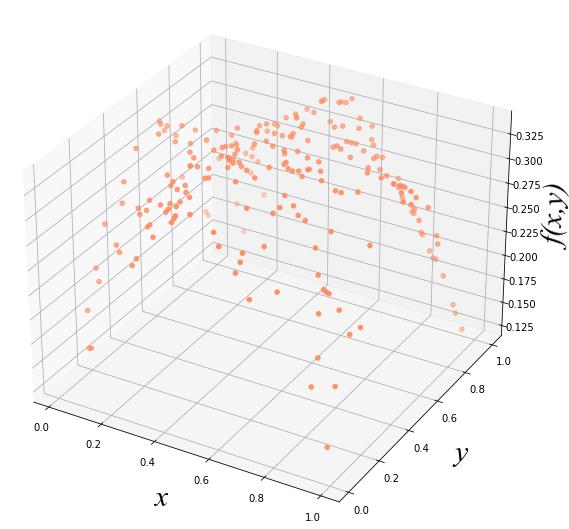
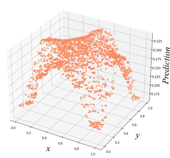
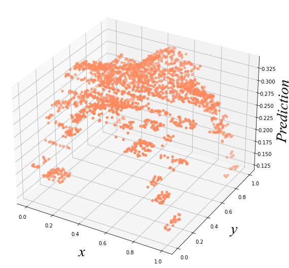
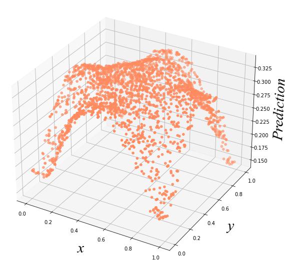
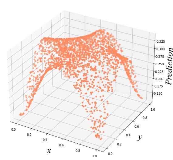
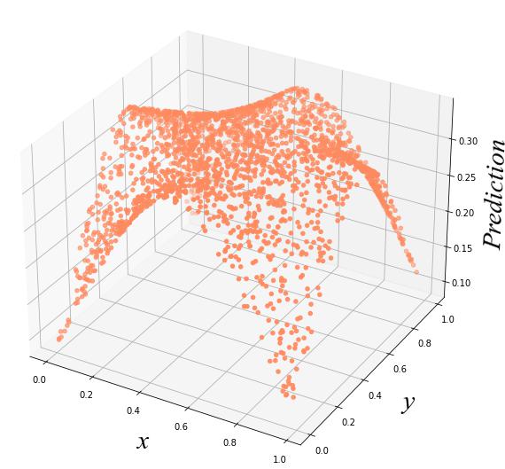
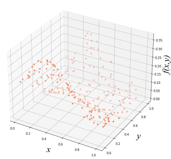
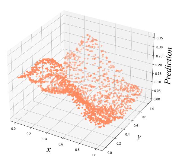
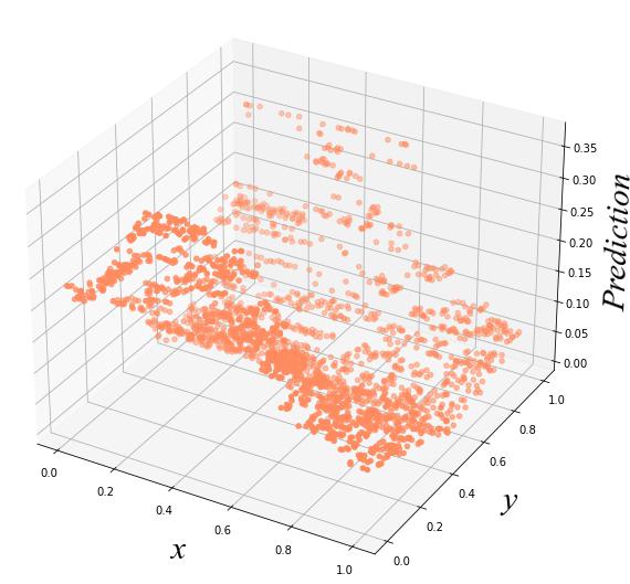
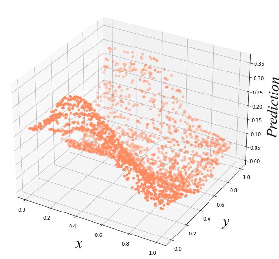
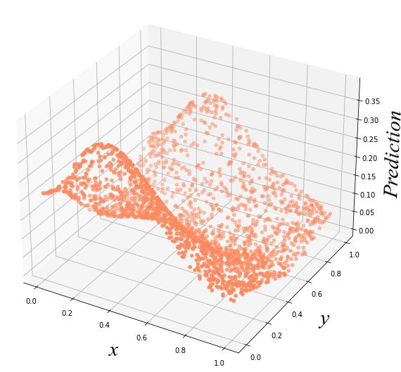
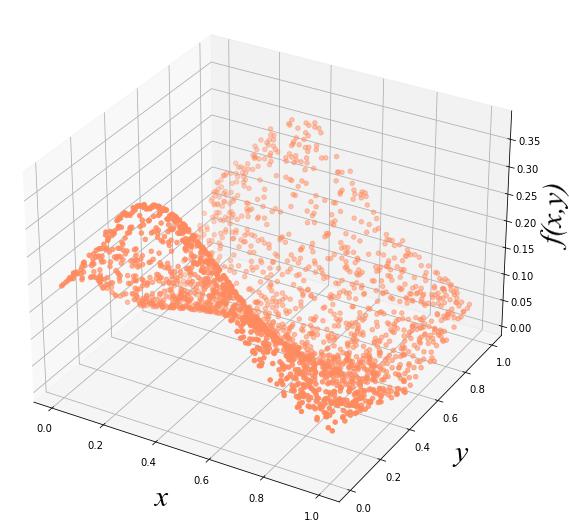
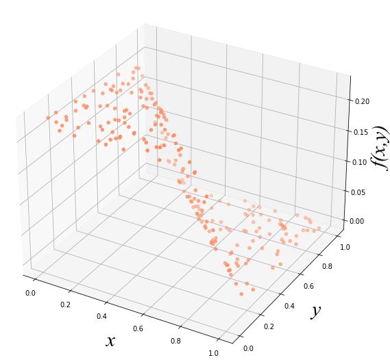
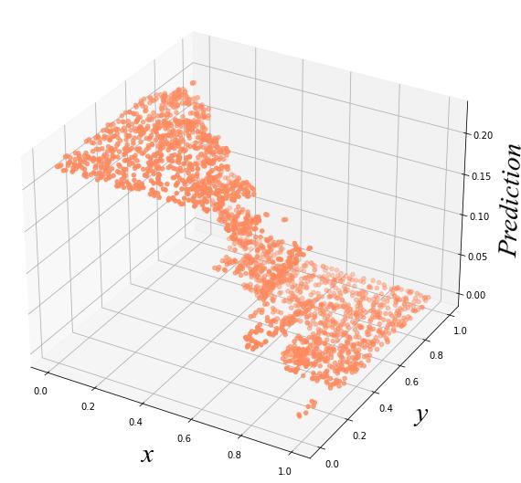
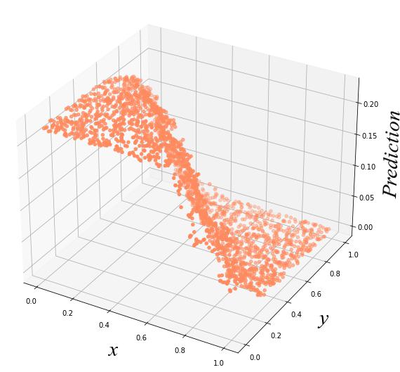
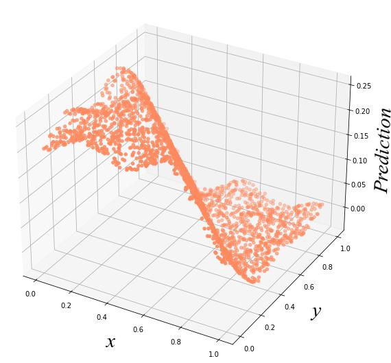
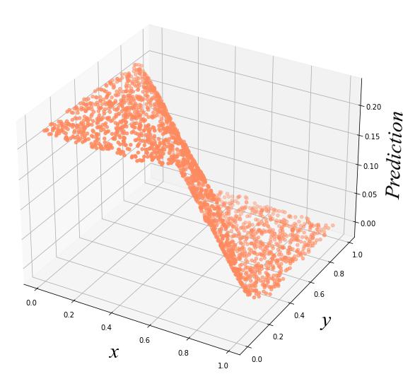
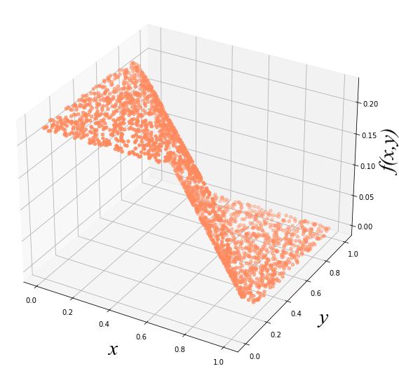
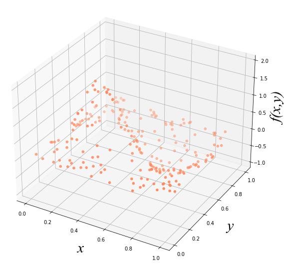
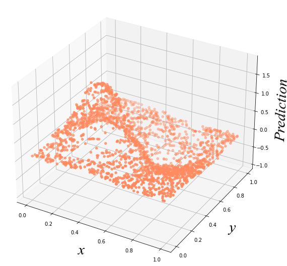
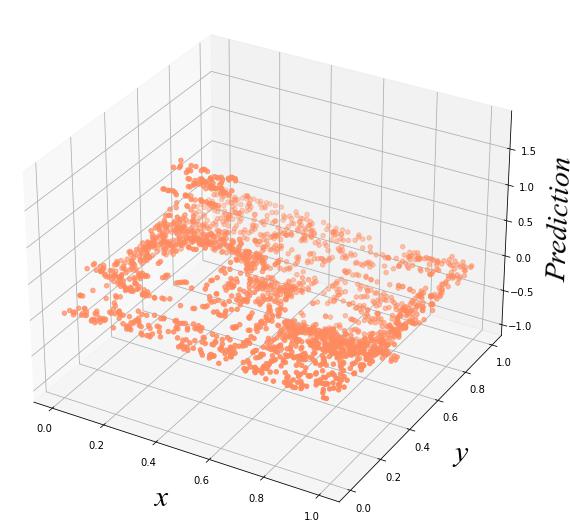
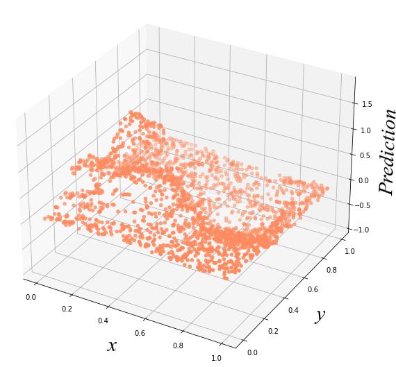
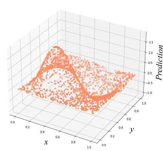
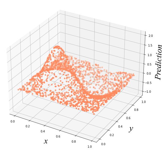
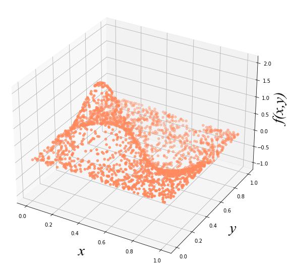
Observed	KNR	DT	RF	FSA-HTF	CRNL	Original

Figure 7: From upper to lower: The results of multivariate regression by different methods on $f_{1}(x,y)$, $f_{2}(x,y)$, $f_{3}(x,y)$, and $f_{4}(x,y)$.

TABLE V: The average quantitative results by different methods for multivariate regression. The best and second-best values are highlighted. (NRMSE $\downarrow$ and R-Square $\uparrow$)

Dataset	Explicit functions									Weather data
	$f_{1}(x,y)$		$f_{2}(x,y)$		$f_{3}(x,y)$		$f_{4}(x,y)$			(55∘N, 117∘W)		(53∘N, 111∘W)		(50∘N, 106∘W)		(47∘N, 100∘W)
Method	NRMSE	R-Square	NRMSE	R-Square	NRMSE	R-Square	NRMSE	R-Square		NRMSE	R-Square	NRMSE	R-Square	NRMSE	R-Square	NRMSE	R-Square
SVR	0.267	0.243	0.499	0.911	0.603	0.940	0.248	0.946		0.076	0.595	0.040	0.442	0.053	0.179	0.051	0.549
KNR	0.044	0.940	0.112	0.963	0.097	0.979	0.189	0.964		0.018	0.949	0.021	0.696	0.027	0.731	0.023	0.806
DT	0.072	0.820	0.152	0.938	0.190	0.919	0.315	0.896		0.023	0.906	0.028	0.533	0.030	0.682	0.030	0.722
RF	0.045	0.930	0.114	0.965	0.118	0.970	0.221	0.953		0.018	0.945	0.024	0.674	0.025	0.760	0.022	0.817
FSA-HTF	0.018	0.989	0.035	0.997	0.069	0.989	0.103	0.989		0.027	0.878	0.038	0.207	0.030	0.683	0.028	0.727
CRNL	0.005	1.000	0.006	1.000	0.018	0.999	0.013	1.000		0.015	0.961	0.022	0.686	0.024	0.779	0.021	0.838

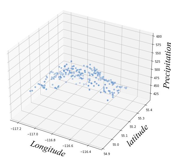
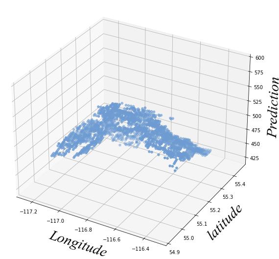
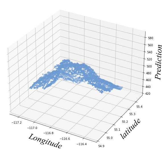
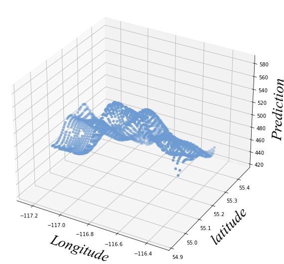
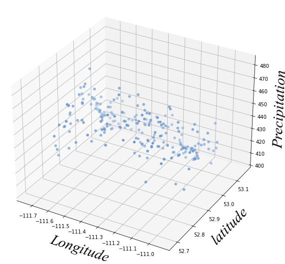
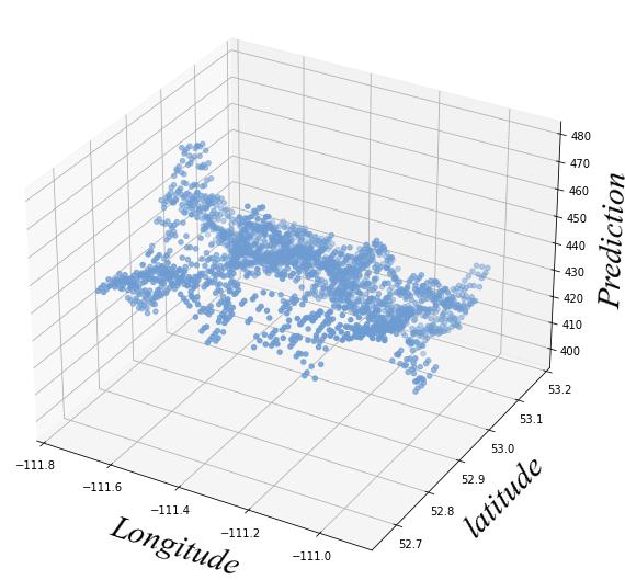
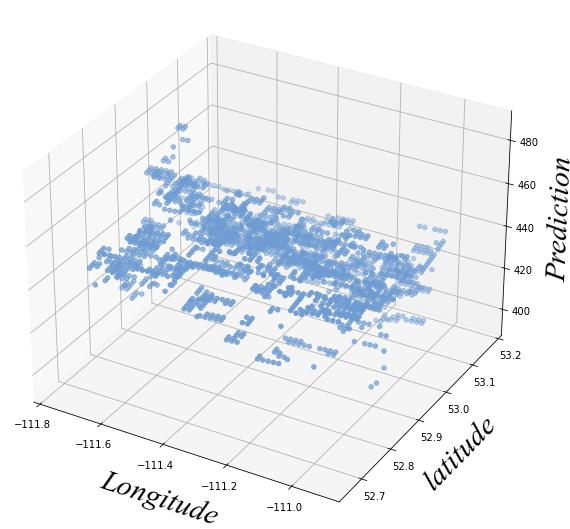
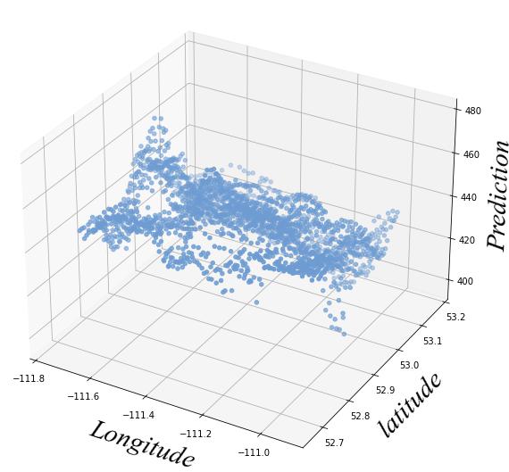
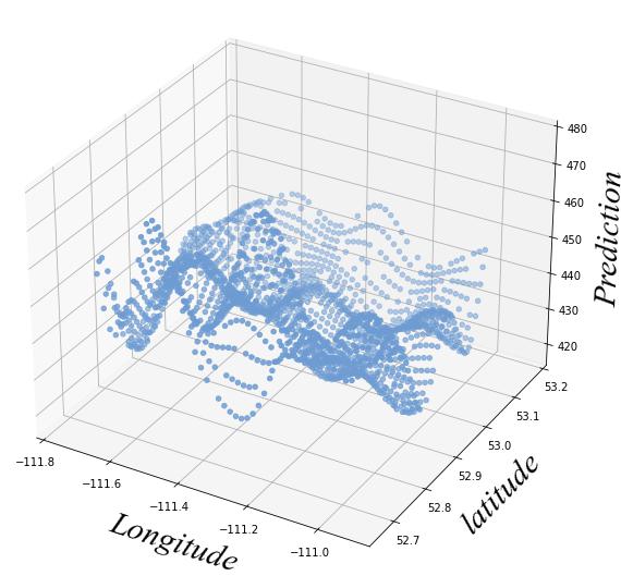
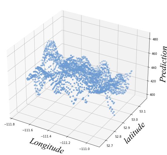
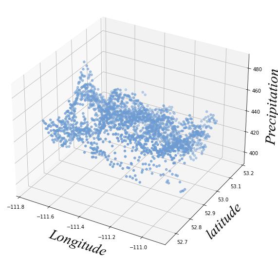
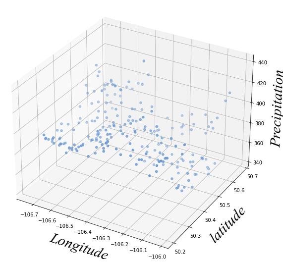
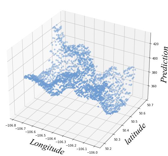
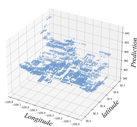
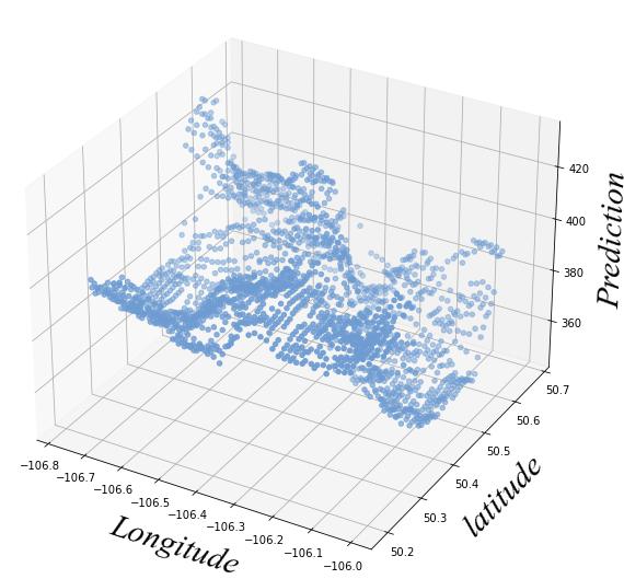
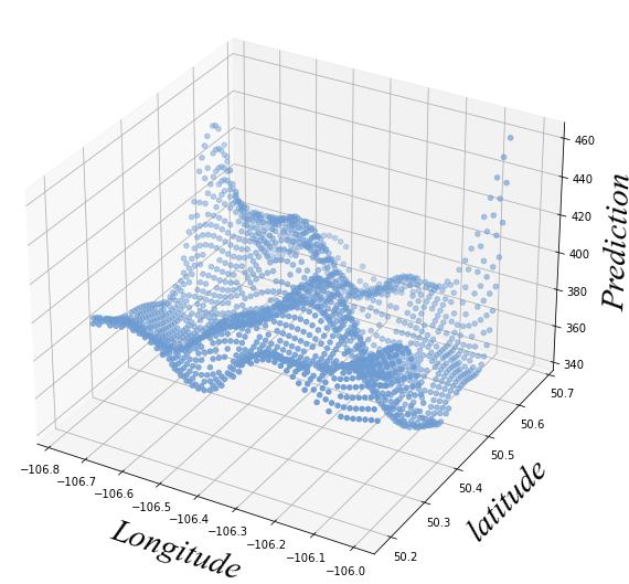
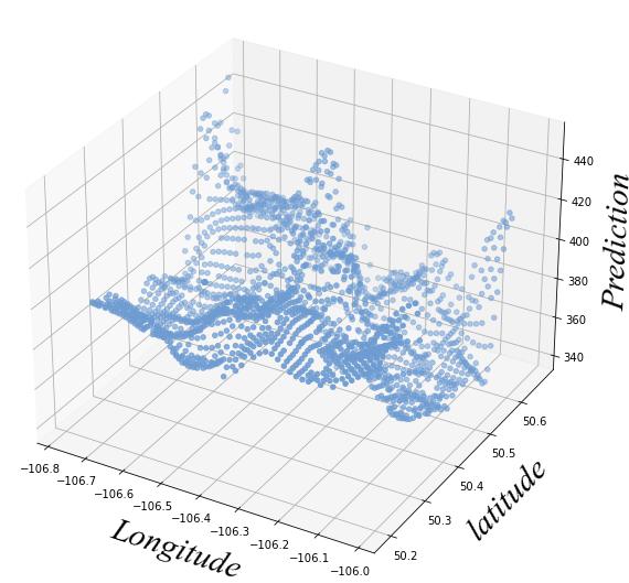
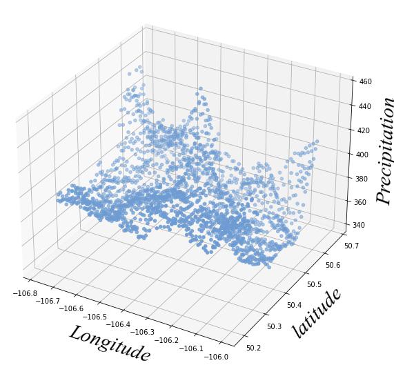
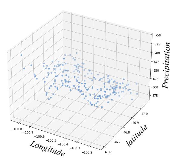
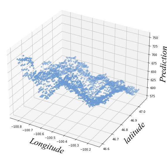
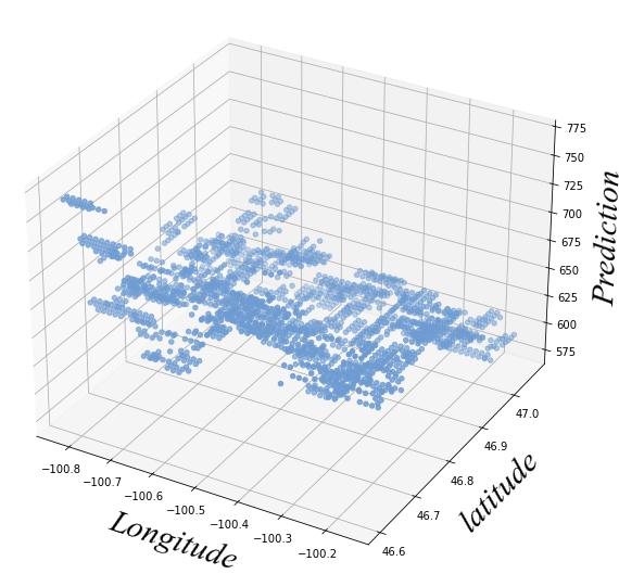
Observed	KNR	DT	RF	FSA-HTF	CRNL	Original

Figure 8: From upper to lower: The results of climate data prediction by different methods on the precipitation data at (55^∘N, 117^∘W), (53^∘N, 111^∘W), (50^∘N, 106^∘W), and (47^∘N, 100^∘W).

IV-C Hyperparameters Settings

Next we introduce the hyperparameters setting. In our method, the hyperparameters are the rank of the coupled low-rank function factorization, i.e., $(r_{1},r_{2},\cdots,r_{N+1})$, the basic continuous cube size, i.e., $p$, and the number of similar cubes, i.e., $S$. We systematically try different hyperparameter values to obtain satisfactory performances. In consequence, we obtain the following hyperparameters settings for different tasks:

• For image inpainting, the rank $(r_{1},r_{2},r_{3},r_{4})$ is set to $(6,6,3,5)$ for color images and $(6,6,{\rm int}(n_{3}/3),5)$ for multispectral images and videos, where $n_{3}$ denotes the size of the third dimension of the observed data. The cube size $p$ is set to 6 for all datasets. The number of similar cubes $S$ is set to 20 for all datasets. The trade-off parameter $\gamma$ of TV regularization is set to $10^{-6}$ for all datasets.

• For image denoising, the rank is set to $(6,6,8,1)$ for all datasets. The cube size $p$ is set to 6 for all datasets. The number of similar cubes $S$ is set to 20 for all datasets. The trade-off parameter $\gamma$ of TV regularization is set to $0.6\times 10^{-5}$ for hyperspectral images and $0.9\times 10^{-5}$ for multispectral images.

• For multivariate regression, the rank $(r_{1},r_{2},r_{3})$ is set to $(15,15,15)$ for synthetic datasets $f_{1}(x,y),\cdots,f_{4}(x,y)$ and climate datasets. For point cloud datasets, the rank $(r_{1},r_{2},r_{3},r_{4},r_{5})$ is set to $(15,15,15,3,10)$. The cube size $p$ is set to 20 for all datasets. The number of similar cubes $S$ is set to 10 for all datasets.

IV-D Experimental Results

IV-D1 Image Inpainting Results

The quantitative and qualitative results of image inpainting are shown in Table III and Figs. 3-4. We can observe that our CRNL generally obtains the best quantitative results as compared with other methods, which verifies the effectiveness of our method for image inpainting. Our NSS-based method enjoys relatively short execution time as compared with other image inpainting methods, which validates the favorable computational efficiency of our method. Meanwhile, from the visual results, we can observe that our method can capture fine details of the images better than other methods, which verifies its strong representation abilities.

IV-D2 Image Denoising Results

The quantitative and qualitative results of image denoising are shown in Table IV and Figs. 5-6. We can observe that our method obtains satisfactory quantitative results as compared with other state-of-the-art methods, including nonlocal low-rank-based methods LTDL and WNLRATV. The superior performance of our CRNL can be rationally attributed to the nonlocal low-rankness and intrinsic similarity within each group and across different groups imposed by our coupled low-rank function factorization, which leads to better noise removal and details recovery. Meanwhile, from the running time comparisons, we can see that our CRNL is quite efficient, especially as compared with classical nonlocal-based methods, e.g., LTDL and WNLRATV, which verifies the favorable computational efficiency of our method due to the coupled function factorization. From the visual comparisons in Figs. 5-6, we can see that our CRNL could generally recover fine details and color information of the images better than other methods, and also remove the noise more thoroughly, which validates the effectiveness of our method for image denoising.

IV-D3 Multivariate Regression Results

The good performances of our CRNL on image inpainting and denoising have demonstrated the effectiveness of our method on classical meshgrid problems. Next, we illustrate the results of multivariate regression tasks. The results on synthetic datasets $f_{1}(x,y),\cdots,f_{4}(x,y)$ and precipitation climate datasets are shown in Table V and Figs. 7-8. We can observe that our CRNL obtains higher accuracy than other methods in most cases. From the visual results in Figs. 7-8, we can see that the results of the proposed method are generally the closest to the true values, especially on the complex climate datasets in Fig. 8, where our method could effectively recover the complex structures of real-world data. These results verify the effectiveness and superiority of our CRNL for data processing beyond meshgrid.

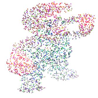
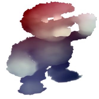
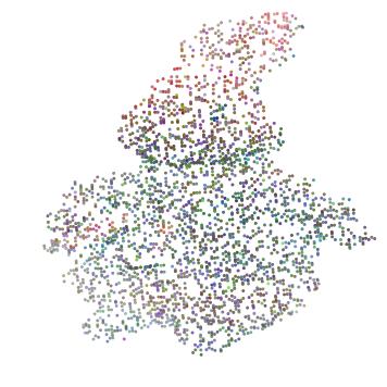
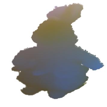
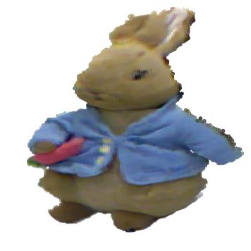
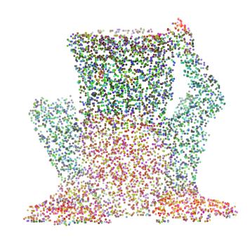
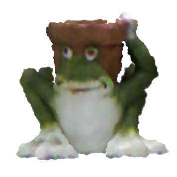
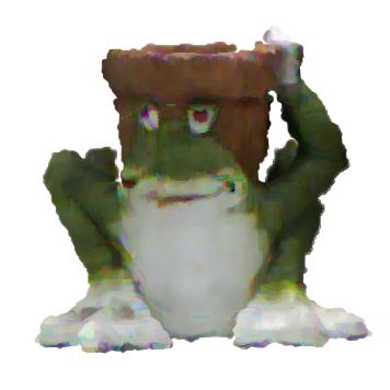
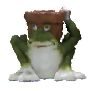
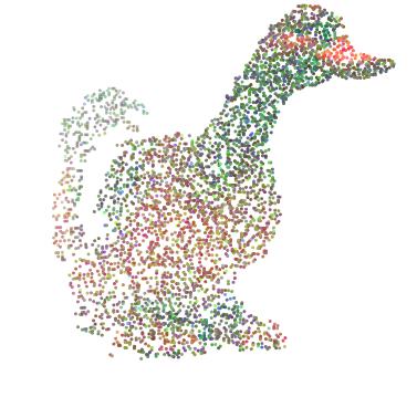
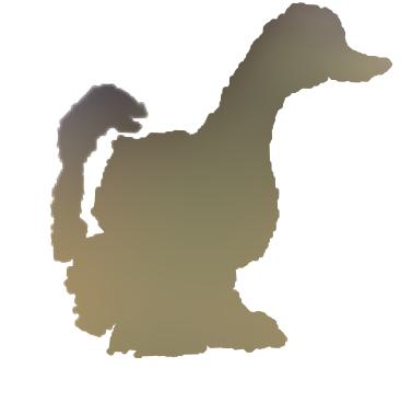
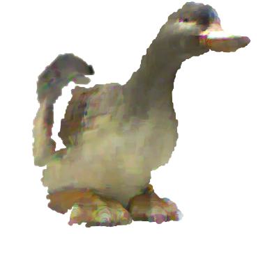
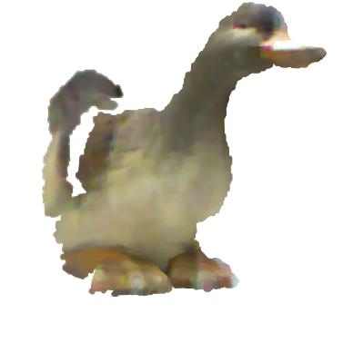
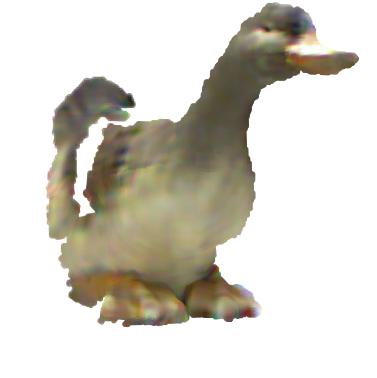
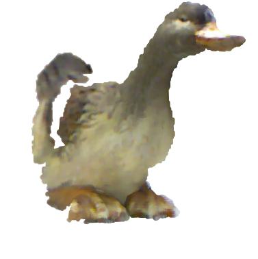
Observed	FSA-HTF	KNR	DT	RF	CRNL	Original

Figure 9: From upper to lower: The results of point cloud recovery by different methods on Mario, Rabbit, Frog, and Duck.

The results of point cloud recovery are shown in Table VI and Fig. 9. Again we can see that our CRNL generally attains better performances than other methods from both quantitative and qualitative perspectives. While FSA-HTF is valid for the former synthetic datasets and climate datasets, it fails to well recover the complex point cloud structures, which is possibly due to its utilized shallow Fourier basis functions. As compared, our CRNL leverages the powerful representation abilities of INRs (i.e., deep neural networks) to parameterize factor functions, which could better capture complex structures of point clouds. The good performances of our method can also be attributed to its elaborate exploration on the nonlocal low-rankness and the similarity within each group and across different groups imposed by the nonlocal coupled low-rank function factorization. In general, the satisfactory performances of our method on different multivariate regression tasks have demonstrated the effectiveness of our method beyond meshgrid.

TABLE VI: The average quantitative results by different methods for point cloud recovery. The best and second-best values are highlighted. (NRMSE $\downarrow$ and R-Square $\uparrow$)

Dataset	Mario		Rabbit		Frog		Duck
Method	NRMSE	R-Square	NRMSE	R-Square	NRMSE	R-Square	NRMSE	R-Square
SVR	0.505	0.207	0.318	0.195	0.365	0.502	0.301	0.062
KNR	0.134	0.936	0.105	0.891	0.082	0.972	0.086	0.922
DT	0.185	0.881	0.148	0.801	0.103	0.957	0.111	0.875
RF	0.139	0.931	0.108	0.887	0.077	0.976	0.085	0.925
FSA-HTF	0.423	0.367	0.281	0.288	0.375	0.418	0.286	0.142
CRNL	0.131	0.937	0.097	0.913	0.072	0.978	0.078	0.922

TABLE VII: The results of image inpainting on color images with sampling rate 0.2 and the corresponding running time (second) by different NSS-based methods.

Dataset	Peppers		Plane		Sailboat		House
Method	PSNR	Time	PSNR	Time	PSNR	Time	PSNR	Time
NL-CP	24.88	9.68	30.04	9.54	23.16	9.36	22.78	10.09
NL-Tucker	22.80	11.58	28.31	11.77	22.37	11.68	21.17	11.71
NL-FCTN	22.13	14.09	29.95	14.10	23.26	17.01	22.52	15.04
CRNL (uncoupled)	25.11	15.66	30.13	15.64	23.38	15.55	22.79	14.50
CRNL (coupled)	25.40	5.73	30.60	5.97	23.67	5.31	23.32	5.51

IV-E Discussions

IV-E1 Advantages of Coupled Function Factorization

As compared with classical NSS-based methods, an important innovation of our method is that we propose the coupled low-rank function factorization to compactly and accurately represent continuous groups with advantageous computational efficiency. To validate these advantages, we consider the proposed method with uncoupled structure, i.e., we use different unshared factor functions to represent different groups. As compared with the original coupled structure (denoted by CRNL (coupled)), the uncoupled low-rank function factorization-based nonlocal method, denoted by CRNL (uncoupled), uses a total of $L\times(N+1)$ factor functions to represent groups, while the original CRNL (coupled) uses only $N+1$ factor functions, where $L$ denotes the number of continuous groups and $N$ denotes the number of dimensions. Hence, CRNL (coupled) is expected to hold much lower computational costs.

We show the comparisons between CRNL (coupled) and CRNL (uncoupled) in Table VII by taking the color image inpainting case as a showing instance. Due to the large memory costs of CRNL (uncoupled), we crop the image size to $100\times 100\times 3$. Meanwhile, we additionally include three baselines: the nonlocal CP tensor decomposition-based method (NL-CP), the nonlocal Tucker tensor decomposition-based method (NL-Tucker), and the nonlocal fully connected tensor decomposition-based method (NL-FCTN)[5]. These three traditional NSS-based methods all employ unshared independent tensor decompositions to parameterize different nonlocal patch groups. For fairness, we implement all methods with GPU calculation on the same platform. From Table VII, we can observe that CRNL (coupled) outperforms other methods including CRNL (uncoupled), and CRNL (coupled) is also more efficient than other NSS methods. Specifically, CRNL (coupled) speeds up the running time about three times against CRNL (uncoupled). The results reveal that the coupled function factorization is indeed helpful to reduce computational costs. Moreover, CRNL (coupled) has better data recovery performance than other nonlocal methods. This is because the coupled function factorization facilitates a beneficial extraction of global correlation knowledge among nonlocal groups intrinsically existed in general on and off-meshgrid data (as shown in Lemma 3). As compared, classical nonlocal methods neglect such helpful information across different groups, and hence CRNL (coupled) is expected to more accurately model the underlying structures of data to achieve better recovery performances.

IV-E2 Sensitivity to Hyperparameters

In this subsection we test the sensitivity of our method to hyperparameters. In our CRNL, the hyperparameters include the rank of the coupled low-rank function representation $(r_{1},r_{2},\cdots,r_{N+1})$, the nonlocal cube size $p$, and the number of similar cubes $S$. By taking the image inpainting task as an example, we test the influence of each of these hyperparameters by changing one of them and fixing the others. The results are shown in Fig. 10. We can observe that our method is relatively robust w.r.t. these hyperparameters, which makes it easy to set suitable hyperparameters in our method and reveals its potential applicability in real scenarios.

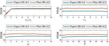
Figure 10: The PSNR values of our method w.r.t. different settings of hyperparameters (The rank $r_{1}$, $r_{2}$, and $r_{4}$, the cube size $p$, and the number of similar cubes $S$) for color image inpainting. Here, we fix the rank $r_{3}$ as the size of the spectral dimension of the color image, i.e., $r_{3}=3$, to ensure a valid result.

V Conclusions

We have proposed the continuous representation-based nonlocal method, or CRNL, for multi-dimensional data processing on and off-meshgrid. Our CRNL first learns a continuous representation of discrete data using INR, and then stack similar continuous cubes into a group. The continuous groups are compactly represented by the coupled low-rank function factorization with shared factor functions and unshared core tensors. By virtue of the coupled function factorization, our CRNL enjoys favorable computational efficiency and finely characterizes the similarity within each group and across different groups. Extensive experiments on-meshgrid (e.g., image inpainting and denoising) and off-meshgrid (e.g., climate data prediction and point cloud recovery) have validated the effectiveness of our method as compared with state-of-the-art methods. In future work, we can consider enhancing the capabilities of CRNL by proven techniques such as iterative regularizations and weighted schemes [3]. Besides, more real-world applications on and off-meshgrid, such as hyperspectral fusion [63] and spherical image processing [64], would be also interesting.

References

- [1] K. Dabov, A. Foi, V. Katkovnik, and K. Egiazarian, “Image denoising by sparse 3-d transform-domain collaborative filtering,” IEEE Transactions on Image Processing, vol. 16, no. 8, pp. 2080–2095, 2007.
- [2] W. Dong, G. Shi, X. Li, Y. Ma, and F. Huang, “Compressive sensing via nonlocal low-rank regularization,” IEEE Transactions on Image Processing, vol. 23, no. 8, pp. 3618–3632, 2014.
- [3] S. Gu, Q. Xie, D. Meng, W. Zuo, X. Feng, and L. Zhang, “Weighted nuclear norm minimization and its applications to low level vision,” International Journal of Computer Vision, vol. 121, p. 183–208, 2017.
- [4] Y. Chen, W. Cao, L. Pang, and X. Cao, “Hyperspectral image denoising with weighted nonlocal low-rank model and adaptive total variation regularization,” IEEE Transactions on Geoscience and Remote Sensing, vol. 60, pp. 1–15, 2022.
- [5] W.-J. Zheng, X.-L. Zhao, Y.-B. Zheng, and Z.-F. Pang, “Nonlocal patch-based fully connected tensor network decomposition for multispectral image inpainting,” IEEE Geoscience and Remote Sensing Letters, vol. 19, pp. 1–5, 2022.
- [6] T.-X. Jiang, M. K. Ng, X.-L. Zhao, and T.-Z. Huang, “Framelet representation of tensor nuclear norm for third-order tensor completion,” IEEE Transactions on Image Processing, vol. 29, pp. 7233–7244, 2020.
- [7] X. Gong, W. Chen, and J. Chen, “A low-rank tensor dictionary learning method for hyperspectral image denoising,” IEEE Transactions on Signal Processing, vol. 68, pp. 1168–1180, 2020.
- [8] Y. Liu, X. Yuan, J. Suo, D. J. Brady, and Q. Dai, “Rank minimization for snapshot compressive imaging,” IEEE Transactions on Pattern Analysis and Machine Intelligence, vol. 41, no. 12, pp. 2990–3006, 2019.
- [9] W. He, H. Zhang, L. Zhang, and H. Shen, “Total-variation-regularized low-rank matrix factorization for hyperspectral image restoration,” IEEE Transactions on Geoscience and Remote Sensing, vol. 54, no. 1, pp. 178–188, 2016.
- [10] J. Peng, Q. Xie, Q. Zhao, Y. Wang, L. Yee, and D. Meng, “Enhanced 3DTV regularization and its applications on hsi denoising and compressed sensing,” IEEE Transactions on Image Processing, vol. 29, pp. 7889–7903, 2020.
- [11] T. Yokota, R. Zdunek, A. Cichocki, and Y. Yamashita, “Smooth nonnegative matrix and tensor factorizations for robust multi-way data analysis,” Signal Processing, vol. 113, pp. 234–249, 2015.
- [12] O. Debals, M. Van Barel, and L. De Lathauwer, “Nonnegative matrix factorization using nonnegative polynomial approximations,” IEEE Signal Processing Letters, vol. 24, no. 7, pp. 948–952, 2017.
- [13] Q. Xie, Q. Zhao, Z. Xu, and D. Meng, “Color and direction-invariant nonlocal self-similarity prior and its application to color image denoising,” Science China Information Sciences, vol. 63, p. 222101, 2020.
- [14] Q. Zhao, P. Tan, Q. Dai, L. Shen, E. Wu, and S. Lin, “A closed-form solution to retinex with nonlocal texture constraints,” IEEE Transactions on Pattern Analysis and Machine Intelligence, vol. 34, no. 7, pp. 1437–1444, 2012.
- [15] X. Zhang, X. Yuan, and L. Carin, “Nonlocal low-rank tensor factor analysis for image restoration,” in IEEE/CVF Conference on Computer Vision and Pattern Recognition (CVPR), 2018, pp. 8232–8241.
- [16] J. Xue, Y. Zhao, W. Liao, and J. C.-W. Chan, “Nonlocal low-rank regularized tensor decomposition for hyperspectral image denoising,” IEEE Transactions on Geoscience and Remote Sensing, vol. 57, no. 7, pp. 5174–5189, 2019.
- [17] Y. Chang, L. Yan, and S. Zhong, “Hyper-laplacian regularized unidirectional low-rank tensor recovery for multispectral image denoising,” in IEEE Conference on Computer Vision and Pattern Recognition (CVPR), 2017, pp. 5901–5909.
- [18] L. Feng, H. Sun, Q. Sun, and G. Xia, “Compressive sensing via nonlocal low-rank tensor regularization,” Neurocomputing, vol. 216, pp. 45–60, 2016.
- [19] L. Wang, Z. Xiong, G. Shi, F. Wu, and W. Zeng, “Adaptive nonlocal sparse representation for dual-camera compressive hyperspectral imaging,” IEEE Transactions on Pattern Analysis and Machine Intelligence, vol. 39, no. 10, pp. 2104–2111, 2017.
- [20] L. Zhang, L. Song, B. Du, and Y. Zhang, “Nonlocal low-rank tensor completion for visual data,” IEEE Transactions on Cybernetics, vol. 51, no. 2, pp. 673–685, 2021.
- [21] Z. Zha, B. Wen, X. Yuan, J. Zhang, J. Zhou, Y. Lu, and C. Zhu, “Nonlocal structured sparsity regularization modeling for hyperspectral image denoising,” IEEE Transactions on Geoscience and Remote Sensing, vol. 61, pp. 1–16, 2023.
- [22] W. Cao, J. Yao, J. Sun, and G. Han, “A tensor-based nonlocal total variation model for multi-channel image recovery,” Signal Processing, vol. 153, pp. 321–335, 2018.
- [23] Y. Wang, T.-Z. Huang, X.-L. Zhao, and T.-X. Jiang, “Video deraining via nonlocal low-rank regularization,” Applied Mathematical Modelling, vol. 79, pp. 896–913, 2020.
- [24] J. Lu, C. Xu, Z. Hu, X. Liu, Q. Jiang, D. Meng, and Z. Lin, “A new nonlocal low-rank regularization method with applications to magnetic resonance image denoising,” Inverse Problems, vol. 38, no. 6, p. 065012, 2022.
- [25] W. Cui, S. Liu, F. Jiang, and D. Zhao, “Image compressed sensing using non-local neural network,” IEEE Transactions on Multimedia, vol. 25, pp. 816–830, 2023.
- [26] Y. Sun, Y. Yang, Q. Liu, J. Chen, X.-T. Yuan, and G. Guo, “Learning non-locally regularized compressed sensing network with half-quadratic splitting,” IEEE Transactions on Multimedia, vol. 22, no. 12, pp. 3236–3248, 2020.
- [27] L. Wang, C. Sun, M. Zhang, Y. Fu, and H. Huang, “Dnu: Deep non-local unrolling for computational spectral imaging,” in IEEE/CVF Conference on Computer Vision and Pattern Recognition (CVPR), 2020, pp. 1658–1668.
- [28] A. Buades, B. Coll, and J.-M. Morel, “A non-local algorithm for image denoising,” in IEEE Computer Society Conference on Computer Vision and Pattern Recognition (CVPR), vol. 2, 2005, pp. 60–65 vol. 2.
- [29] W. Dong, G. Shi, and X. Li, “Nonlocal image restoration with bilateral variance estimation: A low-rank approach,” IEEE Transactions on Image Processing, vol. 22, no. 2, pp. 700–711, 2013.
- [30] X. Liu, X. Chen, J. Li, and Y. Chen, “Nonlocal weighted robust principal component analysis for seismic noise attenuation,” IEEE Transactions on Geoscience and Remote Sensing, vol. 59, no. 2, pp. 1745–1756, 2021.
- [31] L. Zhuang, X. Fu, M. K. Ng, and J. M. Bioucas-Dias, “Hyperspectral image denoising based on global and nonlocal low-rank factorizations,” IEEE Transactions on Geoscience and Remote Sensing, vol. 59, no. 12, pp. 10 438–10 454, 2021.
- [32] H. Chen, M. Wei, Y. Sun, X. Xie, and J. Wang, “Multi-patch collaborative point cloud denoising via low-rank recovery with graph constraint,” IEEE Transactions on Visualization and Computer Graphics, vol. 26, no. 11, pp. 3255–3270, 2020.
- [33] D. Zhu, H. Chen, W. Wang, H. Xie, G. Cheng, M. Wei, J. Wang, and F. L. Wang, “Nonlocal low-rank point cloud denoising for 3-D measurement surfaces,” IEEE Transactions on Instrumentation and Measurement, 2022, doi=10.1109/TIM.2021.3139686.
- [34] M. Imaizumi and K. Hayashi, “Tensor decomposition with smoothness,” in International Conference on Machine Learning (ICML), vol. 70, 2017, pp. 1597–1606.
- [35] N. Kargas and N. D. Sidiropoulos, “Supervised learning and canonical decomposition of multivariate functions,” IEEE Transactions on Signal Processing, vol. 69, pp. 1097–1107, 2021.
- [36] I. V. Oseledets, “Constructive representation of functions in low-rank tensor formats,” Constructive Approximation, vol. 37, pp. 1–18, 2013.
- [37] B. Hashemi and L. N. Trefethen, “Chebfun in three dimensions,” SIAM Journal on Scientific Computing, vol. 39, no. 5, pp. C341–C363, 2017.
- [38] V. Sitzmann, J. Martel, A. Bergman, D. Lindell, and G. Wetzstein, “Implicit neural representations with periodic activation functions,” in Advances in Neural Information Processing Systems (NeurIPS), vol. 33, 2020, pp. 7462–7473.
- [39] J. Lee, J. Tack, N. Lee, and J. Shin, “Meta-learning sparse implicit neural representations,” in Advances in Neural Information Processing Systems (NeurIPS), M. Ranzato, A. Beygelzimer, Y. Dauphin, P. Liang, and J. W. Vaughan, Eds., vol. 34, 2021, pp. 11 769–11 780.
- [40] C. Ma, P. Yu, J. Lu, and J. Zhou, “Recovering realistic details for magnification-arbitrary image super-resolution,” IEEE Transactions on Image Processing, vol. 31, pp. 3669–3683, 2022.
- [41] J. Chibane, T. Alldieck, and G. Pons-Moll, “Implicit functions in feature space for 3D shape reconstruction and completion,” in IEEE/CVF Conference on Computer Vision and Pattern Recognition (CVPR), 2020, pp. 6968–6979.
- [42] W. Zhao, X. Liu, Z. Zhong, J. Jiang, W. Gao, G. Li, and X. Ji, “Self-supervised arbitrary-scale point clouds upsampling via implicit neural representation,” in IEEE/CVF Conference on Computer Vision and Pattern Recognition (CVPR), 2022, pp. 1989–1997.
- [43] Y. Chen, S. Liu, and X. Wang, “Learning continuous image representation with local implicit image function,” in IEEE/CVF Conference on Computer Vision and Pattern Recognition (CVPR), 2021, pp. 8624–8634.
- [44] J. Yang, S. Shen, H. Yue, and K. Li, “Implicit transformer network for screen content image continuous super-resolution,” in Advances in Neural Information Processing Systems (NeurIPS), vol. 34, 2021, pp. 13 304–13 315.
- [45] K. Zhang, D. Zhu, X. Min, and G. Zhai, “Implicit neural representation learning for hyperspectral image super-resolution,” IEEE Transactions on Geoscience and Remote Sensing, vol. 61, pp. 1–12, 2023.
- [46] C. Kim, J. Lee, and J. Shin, “Zero-shot blind image denoising via implicit neural representations,” arXiv:2204.02405, 2022.
- [47] T. G. Kolda and B. W. Bader, “Tensor decompositions and applications,” SIAM Review, vol. 51, no. 3, pp. 455–500, 2009.
- [48] D. Kingma and J. Ba, “Adam: A method for stochastic optimization,” in International Conference on Learning Representations (ICLR), 2015.
- [49] Y. Luo, X. Zhao, Z. Li, M. K. Ng, and D. Meng, “Low-rank tensor function representation for multi-dimensional data recovery,” IEEE Transactions on Pattern Analysis and Machine Intelligence, 2023, 10.1109/TPAMI.2023.3341688.
- [50] Y. Chen, W. He, N. Yokoya, T.-Z. Huang, and X.-L. Zhao, “Nonlocal tensor-ring decomposition for hyperspectral image denoising,” IEEE Transactions on Geoscience and Remote Sensing, vol. 58, no. 2, pp. 1348–1362, 2020.
- [51] L. Yuan, C. Li, D. P. Mandic, J. Cao, and Q. Zhao, “Tensor ring decomposition with rank minimization on latent space: An efficient approach for tensor completion,” in AAAI Conference on Artificial Intelligence (AAAI), 2019, pp. 9151–9158.
- [52] D. Ulyanov, A. Vedaldi, and V. Lempitsky, “Deep image prior,” International Journal of Computer Vision, vol. 128, p. 1867–1888, 2020.
- [53] Y. Luo, X.-L. Zhao, D. Meng, and T.-X. Jiang, “HLRTF: Hierarchical low-rank tensor factorization for inverse problems in multi-dimensional imaging,” in IEEE/CVF Conference on Computer Vision and Pattern Recognition (CVPR), 2022, pp. 19 303–19 312.
- [54] M. Yang, Q. Luo, W. Li, and M. Xiao, “3-D array image data completion by tensor decomposition and nonconvex regularization approach,” IEEE Transactions on Signal Processing, vol. 70, pp. 4291–4304, 2022.
- [55] H. Wang, J. Peng, W. Qin, J. Wang, and D. Meng, “Guaranteed tensor recovery fused low-rankness and smoothness,” IEEE Transactions on Pattern Analysis and Machine Intelligence, 2023, doi=10.1109/TPAMI.2023.3259640.
- [56] F. Yasuma, T. Mitsunaga, D. Iso, and S. K. Nayar, “Generalized assorted pixel camera: Postcapture control of resolution, dynamic range, and spectrum,” IEEE Transactions on Image Processing, vol. 19, no. 9, pp. 2241–2253, 2010.
- [57] Y. Wang, J. Peng, Q. Zhao, Y. Leung, X.-L. Zhao, and D. Meng, “Hyperspectral image restoration via total variation regularized low-rank tensor decomposition,” IEEE Journal of Selected Topics in Applied Earth Observations and Remote Sensing, vol. 11, no. 4, pp. 1227–1243, 2018.
- [58] J. Peng, H. Wang, X. Cao, X. Liu, X. Rui, and D. Meng, “Fast noise removal in hyperspectral images via representative coefficient total variation,” IEEE Transactions on Geoscience and Remote Sensing, vol. 60, pp. 1–17, 2022.
- [59] Q. Yuan, Q. Zhang, J. Li, H. Shen, and L. Zhang, “Hyperspectral image denoising employing a spatial–spectral deep residual convolutional neural network,” IEEE Transactions on Geoscience and Remote Sensing, vol. 57, no. 2, pp. 1205–1218, 2019.
- [60] A. Maffei, J. M. Haut, M. E. Paoletti, J. Plaza, L. Bruzzone, and A. Plaza, “A single model CNN for hyperspectral image denoising,” IEEE Transactions on Geoscience and Remote Sensing, vol. 58, no. 4, pp. 2516–2529, 2020.
- [61] S. Lee, G. Wolberg, and S. Shin, “Scattered data interpolation with multilevel b-splines,” IEEE Transactions on Visualization and Computer Graphics, vol. 3, no. 3, pp. 228–244, 1997.
- [62] Y.-B. Zheng, T.-Z. Huang, X.-L. Zhao, Q. Zhao, and T.-X. Jiang, “Fully-connected tensor network decomposition and its application to higher-order tensor completion,” in AAAI Conference on Artificial Intelligence (AAAI), 2021, pp. 11 071–11 078.
- [63] Q. Xie, M. Zhou, Q. Zhao, Z. Xu, and D. Meng, “MHF-Net: An interpretable deep network for multispectral and hyperspectral image fusion,” IEEE Transactions on Pattern Analysis and Machine Intelligence, vol. 44, no. 3, pp. 1457–1473, 2022.
- [64] J. Li, C. Huang, R. Chan, H. Feng, M. K. Ng, and T. Zeng, “Spherical image inpainting with frame transformation and data-driven prior deep networks,” SIAM Journal on Imaging Sciences, vol. 16, no. 3, pp. 1177–1194, 2023.